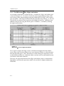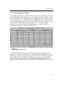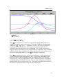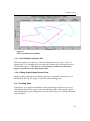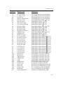
1
A Code for Analyzing Coolant and
Offgas Activity in a Light Water Nuclear
Reactor: Computer Manual
A Code for Analyzing Coolant and Offgas
WARNING:
Please read the Export Control
Agreement on the back cover.
Effective December 6, 2006, this report has been made publicly available in accordance
with Section 734.3(b)(3) and published in accordance with Section 734.7 of the U.S. Export
Administration Regulations. As a result of this publication, this report is subject to only
copyright protection and does not require any license agreement from EPRI. This notice
supersedes the export control restrictions and any proprietary licensed material notices
embedded in the document prior to publication.
CHIRON for WINDOWS – User’s
Manual
A Code for Analyzing Coolant and Offgas Activity in
a Light Water Nuclear Reactor
CM-110056
Computer Manual, June 1998
EPRI Project Manager
B. Cheng
EPRI 3412 Hillview Avenue, Palo Alto, CA 94304, PO Box 10412, Palo Alto, CA 94303, U.S.A. 800.313.3774 or 650.855.2000, www.epri.com
DISCLAIMER OF WARRANTIES AND LIMITATION OF LIABILITIES
THIS REPORT WAS PREPARED BY THE ORGANIZATION(S) NAMED BELOW AS AN
ACCOUNT OF WORK SPONSORED OR COSPONSORED BY THE ELECTRIC POWER
RESEARCH INSTITUTE, INC. (EPRI). NEITHER EPRI, ANY MEMBER OF EPRI, ANY
COSPONSOR, THE ORGANIZATION(S) NAMED BELOW, NOR ANY PERSON ACTING
ON BEHALF OF ANY OF THEM:
(A) MAKES ANY WARRANTY OR REPRESENTATION WHATSOEVER, EXPRESS OR
IMPLIED, (I) WITH RESPECT TO THE USE OF ANY INFORMATION, APPARATUS,
METHOD, PROCESS, OR SIMILAR ITEM DISCLOSED IN THIS REPORT, INCLUDING
MERCHANTABILITY AND FITNESS FOR A PARTICULAR PURPOSE, OR (II) THAT SUCH
USE DOES NOT INFRINGE ON OR INTERFERE WITH PRIVATELY OWNED RIGHTS,
INCLUDING ANY PARTY'S INTELLECTUAL PROPERTY, OR (III) THAT THIS REPORT IS
SUITABLE TO ANY PARTICULAR USER'S CIRCUMSTANCE; OR
(B)
ASSUMES RESPONSIBILITY FOR ANY DAMAGES OR OTHER LIABILITY
WHATSOEVER (INCLUDING ANY CONSEQUENTIAL DAMAGES, EVEN IF EPRI OR ANY
EPRI REPRESENTATIVE HAS BEEN ADVISED OF THE POSSIBILITY OF SUCH
DAMAGES) RESULTING FROM YOUR SELECTION OR USE OF THIS REPORT OR ANY
INFORMATION, APPARATUS, METHOD, PROCESS, OR SIMILAR ITEM DISCLOSED IN
THIS REPORT.
ORGANIZATION(S) THAT PREPARED THIS REPORT
TransWare Enterprises Inc.
ORDERING INFORMATION
Requests for copies of this report should be directed to the EPRI Distribution Center, 207
Coggins Drive, P.O. Box 23205, Pleasant Hill, CA 94523, (510) 934-4212.
Electric Power Research Institute and EPRI are registered service marks of the Electric Power
Research Institute, Inc. EPRI. POWERING PROGRESS is a service mark of the Electric
Power Research Institute, Inc.
Copyright © 1998 Electric Power Research Institute, Inc. All rights reserved.
CITATIONS
This report was prepared by
TransWare Enterprises, Inc.
5450 Thornwood Drive, Suite M
San Jose, California 95123-1222
Principal Investigators
K.E. Watkins
B.D. Paulson
This report describes research sponsored by EPRI.
The report is a corporate document that should be cited in the literature in the following
manner:
CHIRON for WINDOWS—User’s Manual: A Code for Analyzing Coolant and Offgas
Activity in a Light Water Reactor, EPRI, Palo Alto, CA: 1998. CM-110056.
iii
iv
REPORT SUMMARY
The CHIRON code meets the nuclear industry’s need for a model that can estimate the
number of failed fuel rods in the nuclear reactor cores of operating BWRs and PWRs.
This PC-based tool—now available in WINDOWS format—provides this estimate by
using coolant and/or offgas activity measurements. The WINDOWS version adds
significant flexibility in terms of database capabilities and the code’s use as a general
activity release management tool. This user’s manual provides a complete tutorial on
the installation and operation of CHIRON as well as its various outputs.
Background
The CHIRON code for coolant and offgas activity data management and analysis
contains three main elements: a database, a sample analysis module, and a trending
analysis module. The database stores plant design data, cycle operational data, and
activity sample data for multiple cycles along with measurement units and unit
conversion information. The database also stores selected analytical results along with
model parameter settings. The sample analysis module performs a “release-to-birth
versus lambda” least squares fit for determining the number of failed fuel rods in the
core. The trending analysis module provides an overview of the variation of a large
number of measured activities and calculated parameters during a chosen time period.
Objectives
To provide a tutorial for the installation and operation of CHIRON and present an
overview of the code’s enhanced capabilities in the WINDOWS version.
Approach
The project team created a primary user interface featuring enhanced database selection
capabilities, expanded output options, user-defined plant configuration and model
settings, options for setting the units of the input data, and open database analysis
capabilities for user-defined plant cycles. The team also increased the ease of editing
and printing of plots and analysis reports. Finally, they enhanced CHIRON’s potential
for handling a larger number of “reactor- soluble” isotopes as well as an expanded
series of isotopic activity expressions. Each of these changes expands the use of
CHIRON as a general activity release management tool. They created this user’s manual
to support the enhanced CHIRON WINDOWS version.
v
Results
The CHIRON Main Window is the operating base from where control can be passed to
other windows and/or dialog boxes in response to user selections. In specific, CHIRON
features
An extensive BWR/PWR failed fuel database
A general failure model and a combined failure model specifically developed to
address the low power failure problem, with emphasis on identification of the failed
fuel power level
Capabilities for analyzing three groups of fission products, including the noble
gases, the iodines, and the reactor solubles
Use of fitted coefficients in conjunction with coolant sample input
Calculations that include background activity from tramp fuel and recoil
Custom configuration capabilities for individual plants
Capabilities for processing a variety of input data and performing single sample and
batch sample analysis
Outputs of isotopic ratios as well as outputs conforming to requirements of the
Institute of Nuclear Power Operations (INPO) fuel reliability index
Outputs in the form of screen plots and analysis reports for individual samples,
screen plots for trending analysis, and batch export files for transfer of data to a
spreadsheet or alternative applications
This user’s manual provides guidance on the installation of CHIRON 3.0, data entry
methods, and the process for converting previous CHIRON databases. It also describes
forms of output, structure and contents of the CHIRON database, the theory behind
CHIRON calculations, and error message instructions. CHIRON runs on any PC-based
system with WINDOWS 3.1 or higher.
EPRI Perspective
Both the potential and flexibility of the CHIRON 3.0 WINDOWS version have been
significantly enhanced relative to previous DOS versions. Use of this version will enable
utilities to more accurately assess failed fuel rods on a sample-by-sample or batch basis
and produce outputs in a form that will enable them to more effectively manage general
activity releases and fuel failures.
CM-110056
Interest Category
Fuel assembly reliability and performance
Keywords
CHIRON code
LWR
Fuel rods
Failure analysis
Activity release
vi
ABSTRACT
The CHIRON code is a PC based Coolant and Offgas Activity Data Management and
Analysis Tool, now available under WINDOWS. The code contains three main
elements: A database, a sample analysis module, and a trending analysis module. The
database stores plant design data, cycle operational data and activity sample data for
multiple cycles, along with measurement units and unit conversion information. The
sample analysis module performs a “Release-to-Birth versus Lambda” least squares fit,
from which conclusions are made regarding the number of failed fuel rods in the core.
The trending analysis module provides an overview of the variation through a chosen
time period of a large number of measured activities and calculated parameters. A
special calculation provides the Fuel Reliability Indicator, prescribed by the Institute for
Nuclear Power Operations. Selected analytical results are also stored in the database,
along with the model parameter settings used to produce the analyses. CHIRON
accepts keyboard input on a sample-by-sample basis, or batch input from an ASCIIformatted file. Likewise, sample analysis and database storage can be performed in
single-sample or batch mode. The CHIRON output consists of screen plots and analysis
reports for individual samples, screen plots for trending, and batch export files for
transfer of data to a spreadsheet or other alternative application. All plots and text-file
reports can be printed, using the available WINDOWS facilities. The potential and
flexibility of the CHIRON WINDOWS version have been significantly enhanced relative
to previous DOS versions. The capability of the database to handle units and store
model parameter settings along with the samples is one example of an enhancement to
CHIRON. The ease with which editing and printing of plots and analysis reports can be
performed is another. Furthermore, CHIRON now has the potential to handle a larger
number of “reactor soluble” isotopes, as well as an expanded series of isotopic activity
expressions, which greatly expands the use of CHIRON as a general activity release
management tool.
vii
viii
ACKNOWLEDGMENTS
The CHIRON development was initiated by EPRI in 1987, as a logical
continuation of the efforts of the ANS 5.3 Standards Committee. The actual
development of the code was undertaken by S. Levy Incorporated.
We would like to acknowledge the early contributions of Carl Beyer of Battelle
Pacific National Laboratories, who was appointed by the ANS 5.3 Standards
Committee to compile, sort and analyze the initially collected raw data and
advised the S. Levy Incorporated developers.
Wayne Michaels is also acknowledged for his unwavering commitment to and
leadership of CHIRON (MS-DOS version) at S. Levy Incorporated. For
producing the initial Windows version of CHIRON at S. Levy Inc. we want to
acknowledge the efforts of Niels Kjaer-Pedersen and Joe Quintal.
Virginia Jones of TransWare is acknowledged for her efforts in editing the
CHIRON 3.0 User Manual.
Last, but not least, we wish to thank EPRI for supporting the enhancements to
the CHIRON Windows version. The EPRI project managers, Rosa Yang, Odelli
Ozer and Bo Cheng are to be commended for their commitment and
encouragement through the various phases of the CHIRON project.
ix
x
TABLE OF CONTENTS
Section Title
Page No.
1 INTRODUCTION AND OVERVIEW........................................................................1-1
1.1
Identification of Problem ..................................................................................1-1
1.2
Solution Methods .............................................................................................1-1
1.3
Empirical Failure Modeling ..............................................................................1-2
1.4
CHIRON Logic Flow ........................................................................................1-2
1.5
Features and Capabilities ................................................................................1-4
2 GETTING STARTED ..............................................................................................2-1
2.1
System Requirements .....................................................................................2-1
2.2
The CHIRON 3.0 Distribution Package............................................................2-1
2.3
Installing CHIRON from the Diskettes..............................................................2-2
2.4
Description of the Sample Databases............................................................2-11
2.5
Running CHIRON 3.0 Tutorial .......................................................................2-12
3 DATA ENTRY .........................................................................................................3-1
3.1
Data Units (Cardinal Units) ..............................................................................3-1
3.2
Entering Plant Design and Cycle Operational Data .........................................3-2
3.3
Entering New Sample Data Input ....................................................................3-8
3.3.1 Single Sample Activity Data Input ..............................................................3-9
3.3.2 “File Read” (Batch Input) Sample Activity Data Input .................................3-14
4 CHIRON OUTPUT ..................................................................................................4-1
4.1
Single-Sample Screen Plots ............................................................................4-1
4.1.1 The R/B versus
4.1.2 R/B versus
Plot, Offgas and Iodines.................................................4-2
Plot, Solubles ........................................................................4-3
4.1.3 Cs-Ratio versus Predicted Burnup .............................................................4-5
4.1.4 f( ) versus
Plot .........................................................................................4-6
xi
Section Title
4.1.5 C( ) versus
Page No.
Plot .......................................................................................4-7
4.1.6 Failure Correlation Plot...............................................................................4-8
4.1.7 User Defined X Versus Y Plot ....................................................................4-9
4.1.8 Editing Single-Sample Screen Plots...........................................................4-9
4.2
Trending Plots .................................................................................................4-9
4.2.1 Standard Trending Plots...........................................................................4-10
4.2.2 User Defined Trending Plots ....................................................................4-12
4.2.3 Editing Trending Plots ..............................................................................4-12
4.3
Screen Reports..............................................................................................4-12
4.3.1 Offgas Activity Summary Report ..............................................................4-13
4.3.2 Iodines Activity Summary Report .............................................................4-14
4.3.3 Solubles Activity Summary Report ...........................................................4-15
4.3.4 Offgas Release to Birth Summary Report ................................................4-15
4.3.5 Iodines Release to Birth Summary Report ...............................................4-16
4.3.6 Solubles Release to Birth Summary Report .............................................4-17
4.3.7 The Activity Ratio Summary Report .........................................................4-18
4.3.8 The QA Report .........................................................................................4-19
4.3.9 The CHIRON Configuration Screen Report..............................................4-19
4.4
Printed Reports..............................................................................................4-19
4.4.1 The QA Report .........................................................................................4-19
4.4.2 The Calculation Log Report......................................................................4-19
4.4.3 The ASCII Dump Files..............................................................................4-19
5 THE CHIRON DATABASE .....................................................................................5-1
5.1
Database Overview .........................................................................................5-1
5.2
Database Structure..........................................................................................5-1
5.3
Creating a New Database................................................................................5-2
5.4
Compacting a Database ..................................................................................5-3
5.5
Converting a CHIRON 2.3 Database to CHIRON 3.0 ......................................5-4
xii
Section Title
Page No.
6 CHIRON THEORY ..................................................................................................6-1
6.1
FORMULATION OF THE BASIC EQUILIBRIUM EQUATIONS.......................6-1
6.1.1 Least Squares Analysis for Performance Coefficients..............................6-10
6.1.2 Failure Prediction by the “General Failure Models” ..................................6-15
6.1.3 Concentration to Release Rate Conversions ...........................................6-20
6.2
COMBINED FAILURE MODEL......................................................................6-26
6.2.1 Existing Improved Method........................................................................6-26
6.2.2 Improvement Development for CHIRON ..................................................6-27
6.2.3 Operating Plant Observations ..................................................................6-27
6.2.4 Data Analysis ...........................................................................................6-28
6.2.6 Demonstration of Benchmark Fit to Database..........................................6-33
6.3
CHIRON Fuel Failure Database ....................................................................6-37
6.4
The INPO FRI................................................................................................6-38
7 DIAGNOSTICS AND ERROR CHECKING.............................................................7-1
7.1
Data Input Error Messages..............................................................................7-1
7.2
Database Related Error Messages..................................................................7-4
7.3
Miscellaneous Error Messages........................................................................7-7
8 REFERENCES........................................................................................................8-1
A LIST OF FILES INSTALLED BY CHIRON ............................................................ A-1
B FORMAT OF “FILE READ” ASCII FILE ............................................................... B-1
C SAMPLE QA FILE REPORT ................................................................................. C-1
D ASCII DUMP FILES ............................................................................................... D-1
D.1
ASCII Dump File “Chirond0.txt” ...................................................................... D-1
D.2
ASCII Dump File “Chirond1.txt” ...................................................................... D-2
D.3
ASCII Dump File “Chirond2.txt” ...................................................................... D-3
D.4
ASCII Dump File “Chirond3.txt” ...................................................................... D-3
D.5
ASCII Dump File “Chirond4.txt” ...................................................................... D-4
xiii
Section Title
Page No.
D.6
ASCII Dump File “Chirond5.txt” ...................................................................... D-5
D.7
ASCII Dump File “Chirond6.txt” ...................................................................... D-6
D.8
ASCII Dump File “Chirond7.txt” ...................................................................... D-7
D.9
ASCII Dump File “Chirond8.txt” ...................................................................... D-8
D.10 ASCII Dump File “Chirond9.txt” ...................................................................... D-9
E CHIRON DATABASE FORMAT ............................................................................ E-1
xiv
FIGURES
Figure Title
Page No.
Figure 1-1
Figure 2-1
Figure 2-2
Figure 2-3
Figure 2-4
Figure 2-5
Figure 2-6
Figure 2-7
Figure 2-8
Figure 2-9
Figure 2-10
Figure 2-11
Figure 2-12
Figure 2-13
Figure 2-14
Figure 2-15
Figure 2-16
Figure 2-17
Figure 2-18
Figure 2-19
Figure 2-20
Figure 2-21
Figure 2-22
Figure 2-23
Figure 2-24
Figure 2-25
Figure 2-26
Figure 2-27
CHIRON 3.0 Logic Flow Diagram ...........................................................1-3
Welcome to CHIRON 3.0 ........................................................................2-3
Selecting Installation Type ......................................................................2-4
The Data Sources List Box Before Registering Databases.....................2-6
Selecting ODBC Driver ...........................................................................2-7
Data Source Name Definition Box...........................................................2-7
Database File Name Selection Box.........................................................2-8
Registered Database and Driver Designation .........................................2-9
The Data Sources List Box Showing All Databases Required ..............2-10
Setup Complete ....................................................................................2-10
CHIRON Program Group ......................................................................2-11
CHIRON Main Window .........................................................................2-13
CHIRON Main Window – Data Drop-Down Menu .................................2-14
The Data Sources Screen.....................................................................2-14
Output Options Dialog Box....................................................................2-15
The Edit Plant-Cycle Configuration Dialog Box.....................................2-16
The Plant-Cycle Selection Dialog Box...................................................2-17
Sample Select Dialog Box.....................................................................2-18
Box Showing Selected Samples ...........................................................2-19
List of Available Plots ............................................................................2-20
List of Available Reports .......................................................................2-21
Dialog Box for Performing Batch Analysis.............................................2-22
Dialog Box for Trend Plot Selection ......................................................2-22
Anchor Box for Trend Plotting Control...................................................2-23
Time-Select Dialog Box.........................................................................2-23
Trend Plot of Batch Sample Analysis ....................................................2-24
Trending Graph Customization Dialog Box ...........................................2-27
Sample Trend Plot ................................................................................2-28
xv
Figure Title
Page No.
Figure 3-1
Figure 3-2
Figure 3-3
Figure 3-4
Edit Units - Sample Data Units................................................................3-2
Edit Plant-Cycle Configuration Box .........................................................3-3
Add Plant-Cycle Configuration Box.........................................................3-4
New Data Dialog Box ..............................................................................3-9
Figure 3-5
Figure 3-6
Figure 3-7
Sample Data Units Dialog Box..............................................................3-10
Add Sample Data Dialog Box................................................................3-11
Input File Selection................................................................................3-14
Figure 4-1
R/B versus
Figure 4-2
Figure 4-3
R/B versus Plot for Solubles ................................................................4-3
Sample Edit Screen Showing Deletion of Two Cs-Activities ...................4-4
Figure 4-4
Figure 4-5
Figure 4-6
Revised R/B versus Plot for Solubles...................................................4-4
Selection of Burnup Model for Cs-Ratio Burnup Prediction.....................4-5
Cs-Ratio versus Predicted Burnup ..........................................................4-6
Figure 4-7
f( ) versus
Figure 4-8
Figure 4-9
Figure 4-10
Figure 4-11
Figure 4-12
Figure 4-13
Figure 4-14
C( ) versus Plot ....................................................................................4-8
Failure Correlation Plot for BWRs ...........................................................4-9
Offgas Activity Summary Report ...........................................................4-14
Iodines Activity Summary Report ..........................................................4-14
Solubles Activity Summary Report ........................................................4-15
Offgas Release to Birth Summary Report .............................................4-16
Iodines Release to Birth Summary Report ............................................4-17
Figure 4-15
Figure 4-16
Figure 5-1
Figure 5-2
Figure 6-1
Figure 6-2
Figure 7-1
Solubles R/B versus Fit Summary Report ..........................................4-18
Activity Ratio Summary Report .............................................................4-18
ODBC Access Setup Box........................................................................5-3
Compact Database Dialog Box ...............................................................5-4
Combined Failure Model RPF Comparison...........................................6-35
Combined Failure Model Failure Comparison.......................................6-36
Sample CHIRON Error Message ............................................................7-1
xvi
Plot for Offgas and Iodines ................................................4-2
Plot......................................................................................4-7
TABLES
Table Title
Table 2-1
Table 3-1
Table 3-2
Table 6-1
Table 6-2
Table E-1
Table E-2
Table E-3
Table E-4
Table E-5
Table E-6
Page No.
Table of Plot Options.............................................................................2-25
Plant Cycle Configuration Data Entry Options ........................................3-5
Sample Data Input Units .......................................................................3-12
Isotopic Decay Data and Fission Yields ..................................................6-2
Calculation of Rod Power Factor and Number of Failures from
Model ....................................................................................................6-33
Plant Data Table (plant_data) ................................................................ E-1
Sample Data Table (samples)................................................................ E-2
Unit Types Data Table (unit_types)........................................................ E-3
Units Data Table (units) ......................................................................... E-4
User Preferences Data Table (user_preferences) ................................. E-4
Failures Data Table (failures)................................................................. E-5
xvii
1
INTRODUCTION AND OVERVIEW
In this section, a brief overview is given of the problem CHIRON attempts to
solve, the means available for the solution, and the approximations that need to
be made to achieve the solution.
An overview of CHIRON’s notable features and capabilities is also provided in
this section. A flow diagram is included to illustrate the main components of the
CHIRON program and the path the user will follow when using the code.
1.1 Identification of Problem
In the nuclear industry there is a need for a model that can estimate the number
of failed fuel rods in the nuclear reactor cores of boiling water reactors (BWR)
and pressurized water reactors (PWR) during plant operation.
1.2 Solution Methods
CHIRON provides an estimate of the number of failed fuel rods by using coolant
and/or offgas activity measurements. The method of analyzing the activity
samples incorporates a theoretical model of the fission product release
characteristics of chemically similar nuclides (e.g., iodine nuclides and noble gas
nuclides) coupled with an empirical relationship based upon the evaluation of
numerous release samples from various BWR and PWR reactor cycles.
CHIRON performs a failure analysis with the use of two models: the General
Failure Model and the Combined Failure Model. Three groups of fission
products are analyzed by CHIRON. These groups include the noble gases, the
iodines and the reactor solubles. CHIRON has been prepared to include
alternative analyses to handle other subgroups in the future.
The noble gases represent xenon and krypton isotopes for a total of seven
members. The noble gases are frequently referred to in CHIRON as “offgas”,
because of the method by which measurements are obtained in a BWR. This
terminology is used herein to refer to PWR noble gas coolant measurements as
well.
1-1
Introduction and Overview
There are five isotopes that represent the iodine group. Activity measurements
of these isotopes are obtained from analysis of coolant samples in both BWRs
and PWRs.
The reactor solubles consist of a large number of rather dissimilar isotopic
species. These isotopes are partly fission products and partly originating from
environmental impurities or reactor internals. CHIRON does not provide a
direct correlation between the reactor soluble activity measurements and fuel
failures, however, trending of one or more of these nuclides can often be of
benefit in evaluating and tracking various aspects of fuel performance.
1.3 Empirical Failure Modeling
The General Failure Models are based on empirical fits to the large number of
samples in the original database. The data used in the failure correlation was
restricted to reactor power levels above 80 % of rated power, with most of the
data lying near rated power. This is consistent with the fact that most failures
reported during the time span of the database were pellet cladding interaction
(PCI) failures, which tend to occur preferentially at substantial power levels.
Consistently with these benchmarking conditions, the General Failure Models
have proven to work quite well for BWRs, for which failures seem to occur more
frequently at medium to high power levels. Unfortunately, the PWR models
have been somewhat less successful, due to the relatively frequent occurrance of
low power fretting failures. The model improvements for the 1992 version
helped to alleviate this problem, but the most effective approach to predicting
low power failures is the Combined Failure Model, that has been incorporated in
the current version of CHIRON.
The Combined Failure Model was specifically developed to address the low
power failure problem. The specific advantage of this model is the identification
of the failed fuel power level. The model is based on the physical observation
that the isotopic diffusion responds differently to temperature changes for offgas
and iodines. The difference in isotopic diffusion between offgas and iodine
samples has been correlated to fuel failure data over a wide range of rod power
for both BWRs and PWRs. The resulting Combined Failure Model provides
acceptable fuel failure estimates for rod operating conditions that have
traditionally been difficult to evaluate.
1.4 CHIRON Logic Flow
Figure 1-1 shows a simplified flow diagram of CHIRON. The diagram
emphasizes the dataflows, conversions, analyses, and data storage features.
1-2
Introduction and Overview
ODBC
DB-LIST
MAIN WINDOW
CHOOSE
CALC. LOG
& ASCII DUMP
SELECT DATABASES
REGISTERED
DATABASES
OUTPUT OPTIONS
SELECTED DATABASE
PLANT CONFIGURATION
AND MODEL SETTINGS
PLANT
CONFIGURATION
READ IN NEW DATA
SELECT UNITS
MODEL
PARAMETER
SETTINGS
SAVE
FILE INPUT
EDIT UNITS
SCREEN INPUT
OPEN DATA BASE
SELECT PLANT
CYCLE(S)
SELECT FILENAME
FROM LIST
SAMPLE INPUT
SCREEN
SELECTED
INPUT FILE
SAMPLE ANALYSIS
RESULTS SCREEN
SAVE TO DB
EDIT
SELECT SINGLE
SAMPLE
PLOTS
SCREEN REPORTS
VIEW
EDIT
TEXT FILE REPORTS
ANALYZE BATCH
ANALYZE
SELECT MULTIPLE
SAMPLES
IF ASCII DUMP ENABLED,
SPECIFY ASCII DUMP
FILE
ASCII DUMP
OTHERWISE
TREND PLOTS
SAVE TO DB
Figure 1-1
CHIRON 3.0 Logic Flow Diagram
1-3
Introduction and Overview
The primary user interface for CHIRON 3.0 is labeled as the Main Window in the
bold frame on the left of Figure 1-1. From this window, five principal actions
may be taken as described below.
1) Database Selection. CHIRON allows the selection of any one of the
pre-registered databases, connected to the program through the ODBC
interface. The Database Selection is available from the main menu
item “Data”.
2) Output Options. The user may define certain settings that control the
availability of (1) a calculation log file and (2) the feature of exporting
data to an external application (the “ASCII Dump” feature). The
Output Options are available from the main menu item “Options”.
3) Plant Configuration and Model Settings. The user defines the set of
design and operational parameters (the configuration data) that apply
to each plant-cycle to be analyzed. The sets of plant-cycle
configuration data are stored in the database under their plant-cycle
IDs. The Plant Configuration Settings are available from the main
menu item “Options”.
4) Read in New Data. When new sample data is entered into the selected
database, the user is given the option to set the units of the input data.
The units selected will then apply to all subsequently entered samples.
Data may be read in from a data file or it may be entered in screen
form, one sample at a time. In either case, the sample data must refer
to an existing plant-cycle ID configuration. The New Data option is
available from the main menu item “Data”.
5) Open Database. When analyzing sample data , the user may open the
selected database, then proceed to select the plant-cycle(s) for which
samples will be analyzed. If a single sample is selected, the data may
be viewed and edited prior to analyzing. If multiple samples (batch)
are selected, the view/edit option is not available. The analysis data
will always be stored in the database, overwriting any previous
results. When the analysis has been completed, the user may view the
batch analysis results by means of the trend plotting option. The Open
Database option is available from the main menu item “Data”.
1.5 Features and Capabilities
A list of CHIRON’s main features and capabilities is given below.
Extensive BWR/PWR failed fuel database
Uses fitted coefficients in conjunction with coolant sample input
Calculations include background activity from tramp fuel and recoil
Allows custom configuration for individual plants
Handles variety of input data
1-4
Introduction and Overview
Performs single sample and batch sample analysis
Outputs INPO fuel reliability index
Outputs isotopic ratios
Handles data inputs in numerous unit formats – program converts to
standard units used by program
Generates seven different plots
Generates eight different reports
Plots and reports can be viewed on screen
Ability to print plots for presentation purposes
Printable QA reports
WINDOWS provides the code framework in the form of windows and dialog
boxes. The CHIRON Main Window is the operating base from where control can
be passed to other windows and/or dialog boxes in response to the user’s
selections. The windows and dialog boxes are largely self-explanatory, but will
be explained in later sections of this manual.
Detailed instructions on the installation of CHIRON 3.0 and a short tutorial are
provided in Section 2 of this manual. The methods used to enter data into
CHIRON are discussed in Section 3. The various forms of output produced by
CHIRON are presented in Section 4. The structure and contents of the CHIRON
database are described in Section 5. The process for converting previous
CHIRON databases is also discussed in Section 5. Section 6 explains the theory
behind the CHIRON calculations. Section 7 provides a list of error messages
generated by CHIRON and instructions on what to do if you encounter error
messages. References for this manual are contained in Section 8.
This manual also includes several appendices containing useful information on
specific areas of the CHIRON code. Appendix A lists the files that are installed
by CHIRON. Appendix B contains the format for file-read input. Appendix C
shows a sample QA Analysis Report generated by CHIRON. Appendix D
contains the format of the ASCII dump files that are contained on the
distribution disk. Appendix E contains six tables that list the format of the
CHIRON database tables.
1-5
Introduction and Overview
1-6
2
GETTING STARTED
2.1 System Requirements
CHIRON is a 16-bit WINDOWS application, developed under WINDOWS 3.1
with no use of the Win32s libraries. CHIRON 3.0 for WINDOWS runs under
WINDOWS 3.1, WINDOWS 95 and WINDOWS NT operating systems.
The following are the system requirements for installation and efficient use of
CHIRON 3.0 for WINDOWS:
A PC, model 486 or later, with minimum processor speed 50 MHz.
A WINDOWS operating system (3.1x, 95, or NT 4.0).
A VGA monitor or better.
16 MB of RAM.
A hard disk with 15 MB of free space for a “typical” installation.
(The exact requirement will be displayed in a separate screen during the
“custom” installation.)
A 3.5” floppy drive.
The CHIRON distribution package.
2.2 The CHIRON 3.0 Distribution Package
The CHIRON Version 3.0 distribution package consists of a set of three 3.5”
diskettes, one of which is marked “Disk 1 of 3”. This diskette includes the
“Setup” program.
The distribution diskettes include a blank database, “chiblank.mdb”, intended to
form the basis for the user in developing his own, plant-specific database. In
addition, the distribution includes three other databases: “chiron1.mdb”,
“chiron2.mdb” and “chiron3.mdb”. These databases all contain test data
designed to assist the user in getting acquainted with CHIRON and qualifying
the installation.
Getting Started
2.3 Installing CHIRON from the Diskettes
Before starting the installation, the diskettes should be backed up and the backup
copies stored in a safe place. Also close all programs on your WINDOWS system
before starting the installation of CHIRON.
NOTE: These installation instructions are written for a WINDOWS 3.1x user.
All illustrations in this manual represent the image one sees if using CHIRON
3.0 on WINDOWS 3.1x. For those users on WINDOWS NT or WINDOWS 95,
the screens will be the same except for the following: 1) the text in the title
bar will be left justified instead of centered , 2) the symbol used to close a
window and adjust the size of the window are different between WINDOWS
applications. Consult your WINDOWS user manual if you do not know how
to close or adjust the window size in your particular application.
Follow the steps below to install CHIRON 3.0 on your computer.
1. Insert Disk #1, into the 3.5” floppy drive. For a WINDOWS 3.1x installation,
select “File” from the Program Manager, then select “Run” from the dropdown menu. (For WINDOWS NT or WINDOWS 95, from the “Start” menu,
choose Run.) Now, type “a:\setup.exe” into the “Command Line” box, with
“a” representing the floppy drive on your computer. Change the “a” if your
floppy drive is not drive a. Press “Enter” on the keyboard or click “OK” with
your left mouse button.
2. The EPRI CHIRON program banner appears and then the first screen (the
Welcome screen) of the installation process appears. The Welcome screen is
shown in Figure 2-1. Click on “Next” to continue the installation.
2-2
Getting Started
Figure 2-1
Welcome to CHIRON 3.0
3. Choose the destination location for the CHIRON 3.0 program file folder. The
default location is drive C:\CHIRON30. Select an alternate drive if desired.
Click “Next”.
Note: If CHIRON for WINDOWS has been previously installed on the
user’s system, choose the same target directory as the previous installation
so that only one copy of the database will be installed. Folder names are
restricted to eight characters to maintain compatibility with Windows 3.1x.
4. Select the installation type. Figure 2-2 shows the installation types available,
i.e., typical, compact or custom.
2-3
Getting Started
Figure 2-2
Selecting Installation Type
A description of the three types of installation are provided below.
2-4
Typical Installation
All program files, sample database files,
example files, readme files, ODBC drivers, etc.
are installed. It is possible to perform a Typical
Installation on top of an existing installation.
The ODBC database registration will be
performed afer the files are installed. The
database registration can be bypassed by
immediately clicking “Close” in the ODBC
Administrator opening box (the ODBC Data
Sources list box).
Compact Installation
Only the program files, database files and the
readme file are transferred. The database
setup and registration is skipped. Distribution
databases will be overwritten, but their
registration will not be affected. This option
may be useful for installing a new version of
CHIRON, or re-installing the program
executable if this file were to have been
corrupted by system malfunction.
Getting Started
Custom Installation
Any set or sets of files may be chosen for reinstallation. An example of a Custom
Installation would be to reinstall just the
example files. The ODBC driver installation
will be performed, followed by the call to the
ODBC Administrator. By selecting no files to
be transferred, the user is able to perform
maintenance functions on the database system,
such as re-registration of existing databases
under different names, deleting databases from
registration status, or adding databases to the
registered set. It is also possible to perform
database compaction from the ODBC
Administrator. A database can be compacted
into itself, or into a new file to be created.
When ”Custom” installation is chosen, the
setup program will show an extra dialog box,
allowing the user to check the file groups to be
transferred. This screen also shows, for any
selection made, the required disk space along
with the available space on the chosen drive.
It is recommended that “typical” be selected for a first time installation. You
select it by clicking on the radio button next to “typical”.
5. A screen appears telling you that the ODBC and OLE Drivers are being
updated. Click on “Next”.
6. The next step is to select the program folder name. The setup program
suggests the name “CHIRON 3.0” for the program group to appear in the
WINDOWS Program Manager. Accept the default selection by clicking
“Next”.
All the CHIRON program and database files are being copied to the target
directory, along with certain test data files and a readme file. All the CHIRON
“.dll” files, as well as all the required ODBC files (which includes the ODBC
Microsoft Access Driver) are copied to the WINDOWS\SYSTEM directories.
Older versions of these files will be replaced if they exist.
This will take a few minutes. You will see bars on the screen showing the
progress of the installation. You will be asked to insert disks 2 and 3 into the
floppy drive when needed.
NOTE: Should any of the installed .dll files already be found on your
computer system as read only files, the program will prompt you to
overwrite the file. Choose “yes”. Also, if the chosen installation type
requires more disk space than is available on the chosen drive, a message
2-5
Getting Started
will appear, flagging this condition. If this happens, click on “Cancel” to
cancel the installation. A dialog box appears asking if you want to exit
Setup. Click “Exit Setup”. Either free space on the target drive or install
CHIRON 3.0 on a different drive that has more free space.
7. After copying the files, the setup program automatically installs the ODBC
driver, then opens the ODBC Administrator. At this point, the user must
specify how the available databases are to be registered. This is done by
responding to a series of dialog boxes in the ODBC Administrator.
A. After an information box, the first dialog box to appear is the Data
Sources list box as shown in Figure 2-3. During the initial CHIRON
installation this box will probably be empty. It is possible that you have
other programs on your computer that use ODBC and, therefore, have
existing registered data sources. Once databases have been registered,
the list of registered databases will appear in this box whenever you
access this dialog box. Now we are going to add a database so click
“Add”. This opens the next box.
Figure 2-3
The Data Sources List Box Before Registering Databases
B. A list of installed drivers is now displayed as shown in Figure 2-4. Since
the “Microsoft Access Driver” was installed as part of the CHIRON 3.0
installation steps above, it will appear in the list. There may or may not
be other drivers as well, depending on past installations on the computer
system. Select the “Microsoft Access Driver (*.mdb)” by highlighting it
and clicking “OK”.
2-6
Getting Started
Figure 2-4
Selecting ODBC Driver
C. The next box that appears requests the Data Source Name. Enter
“CHIRON DB”. Your screen should look like Figure 2-5. Click “Select”.
NOTE: There must always be a valid database that is registered under
the name “CHIRON DB” for CHIRON 3.0 to function properly. This is
the default Data Source name. On starting up, CHIRON will always
look for a database registered under this name. After starting the
program, the user may select any alternative, registered database.
Figure 2-5
Data Source Name Definition Box
2-7
Getting Started
D. The Database File Name selection box appears next. Under directories,
select the target directory (e.g., C:\CHIRON30). The CHIRON 3.0
installation process places four valid database files: “chiblank.mdb”,
“chiron1.mdb”, “chiron2.mdb” and “chiron3.mdb” in this directory.
Choose the database file “chiron1.mdb” as the Database Name. Your
screen should look like the one shown in Figure 2-6. Click “OK”. This
takes you back to the Data Source name selection box. Note that the
selected database is now C:\CHIRON30\CHIRON1.MDB, assuming you
installed in the sample target directory. Click “OK” again.
Figure 2-6
Database File Name Selection Box
8. The first database, “chiron1.mdb” has now been registered under the Data
Source name “CHIRON DB”, to be used with the “Microsoft Access Driver”.
The name “CHIRON DB” appears in the list of registered databases as shown
in Figure 2-7.
2-8
Getting Started
Figure 2-7
Registered Database and Driver Designation
At this point, it is desirable to add additional databases to the database
registry. Choose “Add” and follow steps 7.B. through 7.D. above again to
register the next database, “chiblank.mdb” as Data Source “CHIBLANK
DB”, to be used with the “Microsoft Access Driver”. (NOTE: The Data
Source name “CHIBLANK DB” is suggested for this example
installation exercise. Any other name compatible with the ODBC
convention may be chosen.) Then, register the remaining two databases
“chiron2.mdb” and “chiron3.mdb” as Data Sources “CHIRON2 DB” and
“CHIRON3 DB”, respectively, to be used with the “Microsoft Access
Driver”.
Verify that all four data source names now appear as shown in Figure 2-8.
Choose “Close” to proceed with the CHIRON installation.
2-9
Getting Started
Figure 2-8
The Data Sources List Box Showing All Databases Required
9. The final installation window appears as shown in Figure 2-9 to indicate that
the setup program is complete. You may be prompted to reboot your
computer now. If so, select “Yes”. Click on “Finish” to complete setup. The
installation program installs several files on your computer system. For a list
of files that are installed, their directory location and purpose, see Appendix
A.
Figure 2-9
Setup Complete
2-10
Getting Started
10. A program group has been created during the installation that contains four
items (see Figure 2-10):
The CHIRON 3.0 Program Icon,
The Database Conversion Program Icon,
The Readme File Icon, and
The Uninstall Icon.
The CHIRON Program Icon is used to start the CHIRON program. The
Database Conversion Program Icon is used when you want to convert
databases from older versions of CHIRON. The process for converting
databases is explained in Section 5. The Readme File Icon accesses the
CHIRON Readme File which contains information which is not found in this
User Manual and that may apply to a specific application of CHIRON. The
Uninstall Icon is used to remove the CHIRON program files from your
computer system.
Figure 2-10
CHIRON Program Group
2.4 Description of the Sample Databases
Included with the CHIRON 3.0 distribution package are four databases: A blank
database, “chiblank.mdb” and three test databases, having filenames
2-11
Getting Started
“chiron1.mdb”, “chiron2.mdb”, and “chiron3.mdb”. The blank database is a preformatted CHIRON database, containing all the empty tables that a user needs to
create his own database. The blank database contains one plant configuration
entry, “Plant-nn”. This entry has been included to serve as a template for
additional entries.
The test databases have the following contents:
“chiron1.mdb”:
Two BWR cycles, Cycles 5 and 7 of Plant “BWR01”
“chiron2.mdb”:
One BWR cycle, Cycle 11 of Plant “BWR02”
“chiron3.mdb”:
One PWR cycle, Cycle 9 of Plant “PWR01”
Additional database files may be created by copying any existing database
(normally the blank database) to a new filename. See Section 5 for details on
how to create a new database in CHIRON.
2.5
Running CHIRON 3.0 Tutorial
This subsection will provide a sample exercise to familiarize you with some of
the CHIRON features and show you how to navigate in the CHIRON windows.
Follow the steps below to learn how to run CHIRON.
Step 1:
Starting CHIRON 3.0
To start CHIRON 3.0, double click on the CHIRON 3.0 for WINDOWS icon in the
WINDOWS Program Manager. A CHIRON 3.0 program banner will appear
briefly followed by the main program window as shown in Figure 2-11.
2-12
Getting Started
Figure 2-11
CHIRON Main Window
Step 2:
Selecting a Database
When CHIRON starts, it automatically opens the database registered under the
default name “CHIRON DB”. If the installation procedure in Subsection 2.3 has
been strictly followed, the selected database is “chiron1.mdb”, containing data
from BWR01 Cycles 5 and 7.
Click on “Data”. The Data drop-down menu appears, see Figure 2-12. Click on
“Select Data Source”.
2-13
Getting Started
Figure 2-12
CHIRON Main Window – Data Drop-Down Menu
The Select Data Source dialog box appears showing the list of registered
databases. Click on Data Source “CHIRON2 DB”, (see Figure 2-13) then click
OK. The program returns to the Main Window.
Figure 2-13
The Data Sources Screen
2-14
Getting Started
Step 3:
Selecting Output Options
From the Main Window select “Options”. Then choose “Output” from the dropdown menu. The dialog box for selecting the output options appears.
In this screen, there are two output options to choose from: 1) a calculation log
file and 2) an ASCII dump file. When selected, the option(s) remains in effect
until changed during a CHIRON session, or until the program is exited. You
may select one, both or none of the options from this box.
1. Enable calculation log file for single sample analysis. If you check this
box, then a text file named “chicalc.log” will be generated at the
completion of each single sample analysis. The “chicalc.log” file will be
placed in the CHIRON30 folder. This file can be used to retrieve all details
of the calculational sequence for the last calculated sample. It may be very
large, on the order of 60 printed pages. This option is not available when
running samples in Batch Analysis mode. Once created, the log-file may
be accessed with the use of a text editor. When a new sample analysis is
performed, the previous chicalc.log file is overwritten. The default choice
for this option is no calculation log file.
2. Enable ASCII Dump files for batch analysis. If you check this box, then
ASCII dump files will be written and placed in the CHIRON30 folder
every time a batch sample analysis is performed. The default choice for
this option is no ASCII Dump file.
For this exercise, click (check) on both boxes. Your screen should look like the
one shown in Figure 2-14. Click OK. The program returns to the main window.
Figure 2-14
Output Options Dialog Box
2-15
Getting Started
Step 4:
Selecting Plant Cycle Configuration
From the CHIRON 3.0 Main Window, click on Options. Select “Plant
Configuration” from the drop-down menu, then select “Edit Existing Plant”. The
Edit Plant-Cycle Configuration dialog box appears. Select “BWR02-11” from the
Plant Cycle ID list in the upper left corner of the box. Notice the data found in
the rest of the box changes to represent the BWR02-11 plant. Now find the place
in the lower right section where “Perform Solubles Calculation” is listed as a
model option. Select it by clicking in the box. Your screen should look like
Figure 2-15. Click OK.
Figure 2-15
The Edit Plant-Cycle Configuration Dialog Box
Step 5:
Select Plant Cycle
Select “Data” from the Main CHIRON 3.0 window, then select “Open”. The
Plant Select dialog box appears as shown in Figure 2-16.
2-16
Getting Started
Figure 2-16
The Plant-Cycle Selection Dialog Box
In this dialog box, there is only one plant name, BWR02, available in the list box.
Highlight the only available cycle (Cycle 11), then click “Select” (the number 11
moves over to the right hand box), then click “OK”.
Step 6:
Selecting Samples to Analyze
The dialog box appears as shown in Figure 2-17. As we go through the exercise
using this box note that there is an extended menu bar at the top containing four
new menu items: Sample, Select, Analysis and Trending. Most of the options
under these menu items may be found on the various buttons on this box. For
instance, the Select menu item contains the “Toggle Status”, “Time-Select Batch”
and “Clear All Selections” options. These options also appear as buttons at the
bottom of the box. Under the Sample menu, there are a few items that are not
found elsewhere on the box. These items include “Delete Sample”, “Delete
Batch” and “Add Sample”. To use any of these particular options, highlight or
mark a sample and then choose the option you desire.
The Sample Select dialog box contains a scrollable list of several hundred
samples. Use the scroll bar on the right side of the table to scroll through the list
of samples. Scroll until the top record in the box is as shown in Figure 2-17.
2-17
Getting Started
Figure 2-17
Sample Select Dialog Box
Use the mouse to first highlight, then x-mark (by clicking the “Toggle Status”
button or by double clicking the mouse button on the sample) the samples dated
8/13/95 at time 20:25:00, 8/14/95 at 20:53:00, and 8/15/95 at 21:18:00. Now, use
the mouse to highlight the sample dated 8/12/95, time 20:30:00.
The screen should now look like Figure 2-18. The list shows that the highlighted
sample has 6 offgas activities, 5 iodines activities, and 7 solubles activities.
2-18
Getting Started
Figure 2-18
Box Showing Selected Samples
Step 7:
Performing Single Analysis of Selected Samples
There are two types of analysis that can be performed: 1) Analyze Single or 2)
Analyze Batch. Analyze Single analyzes the highlighted sample. Analyze Batch
analyzes the X-marked samples only. For this tutorial, choose “Analyze Single”.
The highlighted sample is analyzed. Because the option for “Perform Solubles
Calculation” is set, both offgas/iodines and solubles are analyzed. Note: An
information message may appear that indicates that the Sum of 6 will be used for
this calculation. Click “OK” to continue.
Step 8:
Selecting Plots and Reports
After performing the analysis in Step 7 above, a summary screen report appears.
From the menu bar at the top, either “Plots” or “Reports” can now be selected.
Figure 2-19 shows the drop-down menu list of types of plots that are available in
CHIRON. Click on the various plots to view the result.
2-19
Getting Started
Figure 2-19
List of Available Plots
Figure 2-20 shows the drop-down menu list of types of reports that are available
in CHIRON. Click on the various reports to view the generated report. Detailed
descriptions of CHIRON plots and reports are provided in Chapter 4 of this
document. Close the Fit Summary Report screen by clicking on OK.
2-20
Getting Started
Figure 2-20
List of Available Reports
Step 9:
Performing Batch Analysis and Generating ASCII Dump File
The program goes back to the Samples Select box. Click on “Analyze Batch”.
You will be asked to enter an ASCII Dump Filename. Click “OK” to accept the
default filename, “Chirond”. The three samples selected by x-marks will be
analyzed. A box appears as shown in Figure 2-21 showing the status of the batch
analysis including the record being analyzed and the total number that are
marked for analysis. The box also contains a cancel button to stop the analysis.
2-21
Getting Started
Figure 2-21
Dialog Box for Performing Batch Analysis
Step 10: Creating Trend Plots
After analyzing the selected samples in Step 9 above, the program opens a dialog
box for trend plot selection as shown in Figure 2-22. This dialog box contains two
list boxes, one for the first y-axis, and one for the second y-axis of a dual y-axis
trend plot. Click on the arrow to the right of each box to view the list of choices.
Note that the two lists are identical, but default selections are different. A checkbox is available to select single y-axis plotting, if desired. It is also possible to
cancel trend-plot selection by clicking the “Cancel” button.
Figure 2-22
Dialog Box for Trend Plot Selection
2-22
Getting Started
At this point, cancel the trend plot selection by clicking the “Cancel” button (the
default selection is effective). The program now opens the Trend Plotting
Anchor box (see Figure 2-23). This box offers three choices: “DISPLAY Trend
Graph”, “SELECT Graph Items” and “Cancel”. Choose “Cancel”. Our present
batch sample analysis is too small to produce a meaningful trend plot. We will
increase the number of samples so we can produce a more useful trend plot.
Figure 2-23
Anchor Box for Trend Plotting Control
After selecting “Cancel”, the program goes back to the Samples Select dialog box
(see Figure 2-18). Deselect the previously selected samples by clicking the “Clear
All Selections” button. To get a larger batch selection more suitable for trendplotting, click on the “Time-Select Batch” button. A dialog box opens to permit
the selection of a time period for batch-analysis/trend-plotting (see Figure 2-24).
Figure 2-24
Time-Select Dialog Box
2-23
Getting Started
Enter start date 07/25/95 and end date 08/03/95. Click OK. You are returned to
the Sample Select dialog box. This will select (x-mark) all 36 samples within this
time period. To “thin” the selection, deselect the following samples by
highlighting individually and clicking on the “Toggle Status” button: 7/28/95 at
time 23:10:00, 7/29/95 at 21:02:00, 7/30/95 at 20:18:00, 7/31/95 at 21:10:00,
8/01/95 at 21:05:00, and 8/02/95 at 20:55:00. Click “Analyze Batch” again. An
ASCII dump filename dialog box appears. Then you will see the box showing
the status of the analysis of the samples (similar to Figure 2-21). Next you will
see the trend plot selection screen (Figure 2-22) again.
By default, “Comb. Model Failures” is selected for the Y1 data and “Power” is
selected for the Y2 data. The dialog box also allows the selection of
logarithmic/linear scales, as desired, as well as a moving average range (number
of samples over which to average). The moving average can be applied to all
functions shown in single y-axis plots. Keep the default options, i.e., linear scales
and 7 for running average range. Now press OK. The program returns to the
Trend Plot Anchor box. Select “DISPLAY Trend Graph” to display the selected
trend plot. The plot shown in Figure 2-25 appears.
Figure 2-25
Trend Plot of Batch Sample Analysis
Step 11: Customizing Trend Plots
The trend plot appears with the default options for grid-lines, point markers,
lines/no-lines, etc. Position your mouse anywhere on the graph. Click the right
2-24
Getting Started
mouse button to bring up the menu for customizing your plot. There are several
options available including such things as fonts, grid lines, labels, etc.. Table 2-1
below describes these options.
Table 2-1
Table of Plot Options
List of Options
Description of Function
Viewing Style
Choose the way you want your plot displayed.
Color
Plot will be displayed in color.
Monochrome
Plot will be displayed in monochrome.
Monochrome + Symbols
Plot will be displayed in monchrome + symbols.
Font Size
Choose the font size you want used in your plot
headings and data.
Large
Use large size fonts.
Medium
Use medium size fonts.
Small
Use small size fonts.
Numeric Precision
Choose the numeric precision to be used in plotting
the data points.
No Decimals
Integer numbers used when plotting data points.
1 Decimal
Numbers truncated to one decimal point in plots.
2 Decimals
Numbers truncated to two decimal points in plots.
3 Decimals
Numbers truncated to three decimal points in plots.
Data Shadows
Places a shadow on each data point to increase
visibility.
Grid Lines
Show grid lines on plot display.
Both Y and X Axis
Show grid lines on both axes.
Y Axis
Show grid lines on the Y Axis only.
X Axis
Show grid lines on the X Axis only.
No Grid
Do not show grid lines on the plot display.
Grid in Front
Grid lines appear in front of data points. If a data
point falls directly on a grid line, the data point is
obscured.
2-25
Getting Started
List of Options
Description of Function
Include Data Labels
Unique identifying labels are placed on each data
point. Some plots have data labels designed
specifically for that plot, while others will show
default numeric, sequential data labels.
Mark Data Points
Put dots to mark the data points on the plot. By
default this option is selected.
Show Annotations
Annotations have been set for certain plots. If
annotations are set, they will appear when this is
selected. The user cannot make customized
annotations. By default this option is selected.
Undo Zoom
Display the plot in normal scale.
Maximize
Maximize the size of the plot display.
Customization Dialog
You can edit the various style settings to customize
your plot display. Many of the items found in this
option are available as individual options elsewhere
in this menu, but are repeated here on one menu to
allow you to customize everything at once. There
are many plot styles to choose from such as bar,
area, line, points, etc. See the Help option for
assistance on using all of these options.
General
Plot Style
Subsets
Fonts
Color
Export Dialog
Metafile
Export the plot. Determine the file type for
exporting, the destination for the export and the
object size for exporting.
Export the plot in metafile format.
Bitmap
Export the plot in bitmap format.
Embedded Object
Export the plot in embedded object format.
Text/Data Only
Export the plot in text/data file format.
Export:
Export To:
Clipboard
Export the plot to the clipboard.
File
Export the plot to a file.
Printer
Export the plot to a printer. Choose the size to
print, i.e., full-size or a specified size.
Help
Displays help screen containing a indexed list of
help categories for the options found on this menu.
Find the option you need help with and a detailed
explanation will be provided on the use of the
option.
2-26
Getting Started
To see an example of a couple of these features, start by choosing “Grid Lines”
from the menu. This brings up a submenu. Click on “Both Y and X Axis”. The
plot reappears with gridlines. Now, click the right mouse button again and
choose the “Customization Dialog”. A dialog box appears that has five sheets:
General, Plot Style, Subsets, Font, and Color. Choose the sheet named “Plot
Style”. You will see the screen shown in Figure 2-26.
Figure 2-26
Trending Graph Customization Dialog Box
From that sheet, under “Axes”, choose the y-axis labeled “Comb. Model
Failures”. Under “Plot Style” select “Line”. Next, select another choice under
“Axes”, “Power Frac Pwr”. Select “Line” for Plot Style again. Accept the changes
by clicking “Apply”. To show your action has been applied, the “apply” button
is grayed or disabled now. Then click OK to get back to the plot. The plot has
now changed its appearance as shown in Figure 2-27. Experiment some more to
become familiar with the various options for customizing your plots.
2-27
Getting Started
Figure 2-27
Sample Trend Plot
Two additional features are found in the trend plots and are accessed with the
mouse button. As you move the mouse button on the plot note there is a time
and number shown on the upper left corner of the plot. As you move the mouse,
the number changes. This number identifies the coordinates of the mouse cursor
within the graph area. If you leave the graph area, the number disappears. Also
note that when the mouse is directly on a data point on the graph, a tiny hand
appears so you know you are on a data point and can identify the coordinates
shown in the upper left corner with that point. Put your mouse directly on a
data point and see the tiny hand symbol.
A second feature that is useful when working with plots, is the zoom feature. To
zoom in (magnify) on a particular portion of the plot, click and hold down the
mouse button while moving the mouse over the area you wish to enlarge. A box
will form on the screen indicating the area you are encompassing in your zoom.
When you release the mouse button you see part of the plot in an enlarged state.
When you wish to return to the normal plot state, click on the right mouse button
and select the “undo zoom” option.
2-28
Getting Started
Step 12: Printing
Finally, as a final exercise in trend plots, try printing to an available WINDOWS
printer by performing the following: from the right mouse button menu, choose
the “Export Dialog”. From the Export Dialog choose “MetaFile” as the type of
file you are exporting; “Printer” as the export designation; and “Full Page” as
object size. Click “Print”. A printer configuration box appears. Verify the
printer you are printing to, the paper selection, etc. Click OK. If an appropriate
printer configuration exists under WINDOWS, the plot will be printed.
Step 13: Exiting from CHIRON
Now, close the trend plot by pressing the “Esc” key on the keyboard. The anchor
box reappears. Press “Cancel” to quit trend plotting. On “Cancel”, the program
goes back to the Samples Select dialog box (Figure 2-18). Close this box. The
program goes back to the main window. Select “Exit” under the “Data” menu to
exit from CHIRON.
2-29
Getting Started
2-30
3
DATA ENTRY
This section provides detailed information on the various methods and formats
used to enter new data and edit existing data in the CHIRON 3.0 database. Two
methods of entering new data are supported in CHIRON: screen input and file
input. All data entered into the CHIRON 3.0 database must conform to the
database structure and data units. Data units, data ranges and default values (if
available) for each data type are provided in this section. CHIRON allows the
user to input the numerical values in any numerical format, i.e., decimal, integer,
or exponential.
A data range checking procedure in CHIRON 3.0 performs unit conversions
where appropriate. It also performs certain checks on input data to minimize the
risk of serious numerical problems due to accidentally entered input values that
are dramatically out of range. Tables 3-1 and 3-2 list the acceptable CHIRON data
ranges.
3.1 Data Units (Cardinal Units)
When data is input to CHIRON the user must be sure to use the data units that
are supported by the CHIRON program. Units are defined in the CHIRON
database for each data entry field. A set of reference units, referred to as the
“Cardinal Units” are used internally in CHIRON, as well as for all on-screen
output. In addition, the user selects a set of input units from a pre-defined list of
choices shown in list-boxes on the sample data units screen.
To check the data units currently in effect, perform the following:
From the main window, select “Data”
Click on “New”
Select “Edit Units” from the New Data dialog box. The Sample Data Units
dialog box appears and lists the Cardinal Units for each sample data input
item (see Figure 3-1).
3-1
Data Entry
Figure 3-1
Edit Units – Sample Data Units
The asterisks in parentheses indicate that these are cardinal units that CHIRON
uses internally. CHIRON converts from the selected units to the appropriate
cardinal units, using built-in conversion factors.
Note: CHIRON initially has the cardinal units set as the selected units. As
changes are made to the input units, the selections are saved in the database.
Therefore, the latest choice made will be in force until changed by the user.
3.2 Entering Plant Design and Cycle Operational Data
Prior to entry of new sample data, the user needs to check that the Plant-Cycle ID
exists in the database. This is done by clicking on “Options” from the Main
Window, followed by “Plant Config”, then selecting “Edit Existing Plant”. This
opens the Edit Plant-Cycle Configuration Box as shown in Figure 3-2.
3-2
Data Entry
Figure 3-2
Edit Plant Cycle Configuration Box
Remember, CHIRON always opens the CHIRON DB database initially. In
Section 2.3 when you installed CHIRON you set up CHIRON DB with the
Chiron1.mdb database file. The plant cycles contained in Chiron1.mdb appear in
the Plant Cycle ID list in Figure 3-2.
The Plant-Cycle IDs list box shows all Plant Cycle IDs entered into the database.
If the desired plant-cycle already exists, then its configuration data may be
loaded by selecting the plant-cycle ID from the list-box. The configuration may
be edited and then saved by clicking OK.
If the desired plant-cycle is not found in the current list, then the user must add a
new Plant Cycle ID. To add a new Plant Cycle ID, click “Cancel” to return to the
Main Window. From the Main Window, select “Options”, then choose “Plant
Configuration”, then “Add New Plant” from the drop-down menu. This will
open the Add Plant-Cycle Configuration screen (see Figure 3-3), allowing you to
enter the configuration of a new plant-cycle.
3-3
Data Entry
Figure 3-3
Add Plant-Cycle Configuration Box
Add the data in each box starting with Reactor rated power. Click on the data
field you are entering and type in the appropriate data. Be sure to enter the
data in the units noted in parentheses next to the item, i.e., Reactor rated power
must be entered in MWth units. Table 3-1 provides detail on the Plant Cycle
Configuration data entries, including the acceptable data ranges and any default
values used in the program. Note: Unless otherwise indicated, data values
may be entered in any numeric format, i.e., decimal, integer or exponential.
The program will convert the entries to the Cardinal Units used internally by
the program.
When you click OK, the program performs a range check on each value. If all
values are acceptable, then the data is saved to the database and you are returned
to the CHIRON main window. If you click on the “Cancel” button, then the data
is not saved and you are returned to the CHIRON main window.
3-4
Data Entry
If any data item is out of range, a message will appear showing a list of all items
that are out of range. On clicking OK, the user is returned to the dialog box to fix
the problem(s). No data will be entered into the database until all the required
ranges have been satisfied.
Table 3-1.
Plant Cycle Configuration Data Entry Options
Plant Cycle Config. Data
Data Range
Description
Reactor rated power
0<RatPow 1000
0 in MWth
The reactor rated power.
No. of fuel assemblies in
the core
0<NFAss 2000
The number of fuel assemblies in the
reactor core.
in any numeric
format
Total number of fuel rods
in the core
n2 * NFAss * 0.5
Active fuel length
0<Act FuelL
Nrods n2 *
NFAss * 2
The total number of fuel rods in the
reactor core.
The length of the active fuel.
1000 in cm
Reactor water mass, hot
condition
1.0x10⁵ WM
Fuel rods per assembly
face
For BWRs:
1.0x10¹⁰ in grams
The water mass in the reactor at hot
condition.
The number of fuel rods per assembly
face.
6 n 12
For
PWRs:14 n 20
3-5
Data Entry
Plant Cycle Config. Data
Data Range
Description
Clean-up/let down flow
density
0.5 CUDens 2.0
in g/cc
The cleanup or letdown flow density.
Iodine removal efficiency
0<IEff 1 in
fraction
The Iodine removal efficiency (normally
assumed to be unity) is used to compute
the isotopic loss term caused by the cleanup/letdown system. This value
represents the efficiency of the removal
system (e.g. the ion-exchange beds). This
value may vary slightly over time, but
should remain very close to 1.0
representing 100% removal efficiency.
Offgas removal efficiency
0<OGEff 1
The Offgas removal efficiency (normally
assumed to be unity) is used to compute
the isotopic loss term caused by the cleanup/letdown system. This value
represents the offgas removal efficiency
of the letdown flow system. This value
may vary slightly over time, but should
remain very close to 1.0 representing
100% removal efficiency.
in fraction
Rx solubles removal
efficiency
0<RxEff 1
in fraction
3-6
The Rx solubles removal efficiency
(normally assumed to be unity) is used to
compute the isotopic loss term caused by
the clean-up/letdown system. This value
represents the efficiency of the removal
system (e.g. the ion-exchange beds). This
value may vary slightly over time, but
should remain very close to 1.0
representing 100% removal efficiency.
Data Entry
Plant Cycle Config. Data
Data Range
Description
Loop on fission yield
If this option is selected, CHIRON
239
performs an iteration on the Pu fission
yield ratio for the failed fuel. CHIRON
searches for the fission yield that
provides the best overall statistical fit. If
the option is not selected, the user must
supply a value for the yield ratio (see
239
Default Pu frac ).
Calculate tramp yield
If this option is selected, CHIRON sets
the Pu239 fission yield ratio for the tramp
to be equal to the value for the failed fuel.
If the option is not selected, the user must
supply a value for the yield ratio (see
Tramp Yield frac).
Perform solubles
calculation
If this option is selected, CHIRON
performs a least squares fit of up to 15
“solubles” activities. Np239 is not
included, since it is not a fission product.
Default Pu239 frac.
0 PuFrac 1.0
Tramp yield fraction
Tramp recoil frac.
If the “Loop on fission yield” option is
not selected, CHIRON will use the value
specified here for the Pu239 fission yield
ratio for the failed fuel.
If the “Calculate tramp yield” option is
not selected, CHIRON will use the value
specified here for the Pu fission yield
ratio for the tramp.
0<TrRecFrac 1
The value specified here is the fraction of
the tramp for which the fission products
generated are directly released into the
coolant. For normal tramp levels, 1.0
should be used. For very high tramp
levels, a value less than unity may be
specified.
3-7
Data Entry
Plant Cycle Config. Data
Data Range
Description
Convergence limit
1.0x10⁻⁸ Crit 1
The value specified here is the maximum
error in the coefficients allowed for a
valid solution.
Maximum loops
0<Nloops 10000
The value specified here is the maximum
number of iteration loops permitted for
the least squares fitting routine.
epsilon_0
10-8 epsilon_0
The value specified here is used as a
default epsilon in the Combined Failure
Model, when a “Three-Coefficient Fit”
has resulted from the least squares fitting
routine.
10-2
Fuel microstructure
0.1 Fmic 100
The value specified here characterizes the
fission product diffusivity of the failed
fuel. For US-made fuel the recommended
value is unity. For certain foreign made
fuel types, especially fuel made by the
AUC process, the value may be higher.
3.3 Entering New Sample Data Input
CHIRON supports two methods for entering new sample data: 1) the data entry
dialog box or 2) the file-read option. Before loading any sample data it is
important to first enter the Plant Cycle ID using the plant cycle configuration
screen. This procedure is described in Section 3.1 above. Entry of new sample
data into CHIRON starts from the CHIRON main window. Select “Data” and
then “New” from the drop-down menu. This brings up the New Data dialog box
as shown in Figure 3-4.
3-8
Data Entry
Figure 3-4
New Data Dialog Box
The input methods available for entering new sample data are “Screen” and
“File”, selectable by the radio-buttons. “Screen” is intended for single sample
input, “File” for multiple sample (batch) input. The following subsections deal
with each of these input methods separately.
3.3.1 Single Sample Activity Data Input
Before entering sample data, verify the data units that are currently in effect. To
do this, click on “Edit Units”. The Sample Data Units dialog box appears (see
Figure 3-5).
3-9
Data Entry
Figure 3-5
Sample Data Units Dialog Box
If the input units shown in the list-boxes of the Sample Data Units dialog box are
the ones desired then the box is closed by clicking “Cancel”. Otherwise, alternate
units may be selected by holding down on the arrow next to each data unit. In
the case shown in Figure 3-5, the list-box for Reactor Power Units has been
opened. The available choices are shown in the scroll list and include: “FracP”
for fractional power (normally between 0 and 1), “%P” for percent power
(normally between 0 and 100), and “MWth” for absolute power in MWth. The
asterisks in parentheses indicate that these are cardinal units that CHIRON uses
internally. CHIRON converts from the selected units to the appropriate cardinal
units, using built-in conversion factors.
If changes are made to any of the items in the Sample Data Units dialog box, click
OK to accept the changes. Choose “Cancel” to go back to the New Data screen
without accepting any changes.
Now you are ready to enter data. To enter Single Sample Input, click “Screen”
from the New Data dialog box, then OK. The Add Sample dialog box appears as
shown in Figure 3-6.
3-10
Data Entry
Figure 3-6
Add Sample Dialog Box
Input units are shown by each value to remind the user of the current settings.
Table 3-2 provides definitions for the sample data entry fields entered on this
screen.
3-11
Data Entry
Table 3-2.
Sample Data Input Units
Sample Data Input
Data Range
Description
Plant Cycle ID
xxxxx-nn
The Plant Cycle ID must coincide with one
available in the database. Its format is a 5character text-string (Plant Name), followed by
a hyphen (“-”), followed by a single or double
digit number (Cycle Number). The plant name
is case sensitive. Do not use a leading zero in a
single digit cycle number.
Sample Date
mm/dd/yy
The sample date entered in the form
MM/DD/YY.
Sample Time
hh:mm:ss
The sample time entered in the form
HH:MM:SS.
Reactor Power
0 RxPow 10 in
FracP
The current reactor power (as opposed to rated
power).
Clean-up Flow
0< ClFlow 10000
in gal/min
The cleanup or letdown flow rate (required for
conversion of Ci/ml to Ci/sec).
Rod Power Factor
0<RPF 10
The ratio of the linear heat-rating of the failed
fuel, if any, to the average linear heat rating of
the entire core, at the current reactor power level.
For File Read input, occurrences of RPF = 0 will
be replaced by the default value 1.08.
Burnup
0 BU 1000 in
MWd/kgU
An estimate of the burnup of the failed fuel.
Gas Delay Time
-5000 DelTime
50000 in seconds
Any delay that may occur between activity
release for offgas isotopes at the fuel breach,
and sample capture. The delay due to coolant
circulation time is usually negligible.
3-12
Data Entry
Sample Data Input
Data Range
Description
I Delay Time
-5000 DelTime
50000 in seconds
Applies to the iodines, and is otherwise defined
as above for the offgas isotopes.
Sol Delay Time
-5000 DelTime
50000 in seconds
Applies to the reactor solubles, and is otherwise
defined as above for the offgas isotopes.
SJAE (Steam Jet Air For BWRs:
Ejector) Gas Flow
500 SJAEFlow
50000 in cc/sec
For PWRs:
SJAEFlow=0
Offgas Activities
volumetric units:
0 Abs VolOGAct
1.e6 in Ci/cc
release-rate units:
0 Abs RrOGAct
5.e8 in Ci/sec
Iodine Activities
volumetric units:
0 Abs VolIOAct
1.e6 in Ci/cc
release-rate units:
0 Abs RrIOAct
5.e8 in Ci/sec
Rx Solubles
Activities
volumetric units:
0 VolSolAct 1.e6
in Ci/cc
The flow rate of the steam in the bypass line
that drives the evacuation of non-condensable
gases from the condenser, by means of a jet
nozzle. The flow rate is used for BWRs as a
conversion factor between measured activity in
Ci/cc and release rate activity in Ci/sec.
Measured activity of the offgas or noble gas
isotopes. A negative value for an isotopic
activity has the effect of omitting the activity
value from the R/B fit and subsequent fuel
failure evaluations, although the measurement
value is retained in the CHIRON database for
reference purposes.
Measured activity of the iodine isotopes. A
negative value for an isotopic activity has the
effect of omitting the activity value from the
R/B fit and subsequent fuel failure evaluations,
although the measurement value is retained in
the CHIRON database for reference purposes.
Measured activity of the selected reactor
soluble isotopes. Reactor solubles cannot be
included in R/B fit and, therefore, are always
non-negative values.
release-rate units:
0 RrSolAct 5.e8
in Ci/sec
3-13
Data Entry
Click on each data entry field and type in your data. When all data has been
entered into the screen, clicking on “Enter” at the bottom of the screen will save
the data to the database. The user will then be asked if he wants to add another
sample.
For individual sample input, the range checking is performed in the “Add
Sample” screen and the “Edit Sample” screen. The check is performed when the
“Enter” or “OK” button is clicked, respectively. If any data item is out of range, a
message will appear showing a list of all items that are out of range. On clicking
OK, the user is returned to the dialog box to fix the problem(s). No data will be
entered into the database until all the required ranges have been satisfied.
3.3.2 “File Read” (Batch Input) Sample Activity Data Input
Batch, or “File Read” input is selected by the radio button “File” in the New Data
screen (see Figure 3-4).
Selecting “File” brings up the Input File Selection Screen, as shown in Figure 3-7.
You select an input file and click OK. Note: The files read must be formatted as
described in Appendix B. (If you wish to try this feature, an example input file,
“dbcon09.txt”, is provided on the CHIRON 3.0 distribution disk. Click on this
file if desired.)
Figure 3-7
Input File Selection
The selected file is then read into CHIRON. A box appears that shows the line
count as the file is being read. Note: The count indicates the total number of lines
read from the file, including comment lines, i.e., not just the number of data
samples. For “File Read” input, range checking is performed for each record
3-14
Data Entry
read, and any non-compliances are posted to the screen as they occur. In such
cases, the user is advised of the problem and given the choice to either stop the
read-in or to continue. None of the non-compliant records are transferred to the
database.
If the file is read successfully, a list-box appears to show only the newly entered
samples. This box is equivalent to the Samples Selection Box of Figure 2-17.
Samples analysis may proceed from this box, in the manner previously explained
in Section 2.5, Step 9 .To generate a list box containing all samples for the cycle,
close this box and open the plant cycle again (see Section 2.5, Step 5).
Alternatively, batch input files may be created by organizing sample data in a
spreadsheet, such as Microsoft Excel, according to the format shown in
Appendix B, then saving the spreadsheet as a comma-separated text file using
the “Save As” option from the spreadsheet file menu.
3-15
Data Entry
3-16
4
CHIRON OUTPUT
This section discusses the various output produced by CHIRON. With CHIRON
the user can generate single-sample screen plots, various trending plots, screen
reports and printed reports. Descriptions of the plot and report options are
described in the subsections that follow. Illustrations of each type of plot and
report are provided.
Plots and reports can be edited, copied to hard-disk as a bit-map file and/or
printed to any printer installed under WINDOWS. By clicking on the right
mouse button from anywhere inside a graph display, the user can access a menu
containing numerous graphic display options that allow customization of the
CHIRON plot. The user can modify the gridlines, font size, color, data labels,
and more. Printing is controlled from the Export Dialog option, while editing is
normally performed from the Customization Dialog option. A description of
these plot options is provided in Section 2 in Table 2-1. By clicking on the “Help”
option in the right mouse button menu, you can also access more information on
these plot options.
4.1 Single-Sample Screen Plots
The list of available single-sample screen plots is shown below:
Release to Birth (R/B) vs. Lambda for Offgas and Iodines
R/B vs. Lambda for Solubles
Cesium Ratio vs. Predicted Burnup
F(Epsilon) vs. Epsilon
C vs. Epsilon
Failure Correlation Epsilon vs. A Epsilon
Y versus X plot
These plots are accessed from the drop-down menu of the Analysis Summary
screen (see Figure 2-19). The following subsections explain each plot in detail
and provide illustrations of sample plots.
4-1
CHIRON Output
4.1.1 The R/B versus
Plot, Offgas and Iodines
An example of the Release to Birth (R/B) vs. Lambda for offgas and iodines plot
is shown in Figure 4-1. It contains a base-line curve (representing tramp) and a
total activity curve (representing tramp plus failed fuel) for offgas, and a similar
pair for iodines. The separation between the total and tramp activity, i.e., the rise
of the R/B over the base-line, represents the failed fuel activity. Gridlines were
added to this plot by using the menu option “Gridlines”, available by clicking
the right mouse button.
Figure 4-1
R/B versus
Plot for Offgas and Iodines
For a typical sample, the offgas curves will tend to be higher than the iodines
curves, due to the fact that iodines have more chemical affinity to other elements
than do the noble gases. Thus, the behavior of the noble gases represent a close
to ideal diffusion behavior, while the iodine activities may be attenuated because
of reactions with other materials.
However, the separation between the offgas and iodines curves is temperature
dependent, such that the separation tends to be smaller for higher temperature
failed fuel.
4-2
CHIRON Output
4.1.2 R/B versus
Plot, Solubles
An example of the R/B vs. Lambda for Solubles plot is shown in Figure 4-2. The
239
original CHIRON solubles group consists of 15 fission products plus Np . Only
the fission products are used in the R/B versus fitting routine. In the example,
it is seen that the scatter of the points for the solubles group is such that no clear
trend is indicated by the plot. This is fairly typical of the solubles analysis, and is
of little overall value in fuel failure assessment. As a result, the solubles
calculation is optional (selected in the Model Options section of the Plant
Configuration dialog box illustrated in Figure 3-3).
Figure 4-2
R/B versus
Plot for Solubles
A significantly improved analysis can be obtained from the solubles, if the
isotopes Cs134 and Cs137 are omitted. This can be done by bringing up the Sample
Edit dialog box, then changing the sign of the Cs134 and Cs137 activities to negative,
then clicking “OK” (see Figure 4-3, the negative values appear in red on the
screen). This has the effect that these activities will be ignored in the least
squares fit of the sample analysis. The result of the revised fit is shown in Figure
4-4.
4-3
CHIRON Output
Figure 4-3
Sample Edit Screen Showing Deletion of Two Cs-Activities
Figure 4-4
Revised R/B versus
Plot for Solubles
It is envisaged that specific scenarios exist in which solubles analyses will prove
very valuable, in particular when applied to certain subsets of solubles. Further
4-4
CHIRON Output
development is anticipated in this area. For the present, however, it is
recommended that the solubles analysis be switched off for routine analyses.
This is the default choice in the Add Plant Configuration dialog box, see Figure
3-3).
4.1.3 Cs-Ratio versus Predicted Burnup
134
137
The ratio of the two cesium activities Cs and Cs can be used to estimate the
burnup of the failed fuel. When the Cs-ratio burnup plot is chosen, the dialog
box shown in Figure 4-5 appears.
Figure 4-5
Selection of Burnup Model for Cs-Ratio Burnup Prediction
The user may now select a “Plant Cycle History”. The Plant Cycle History refers
to a set of reference ORIGEN curves that are dependent on the plant type, cycle
length, outage schedule, enrichment, and reactor power. These curves are
available to compare the Cs ratio calculated by CHIRON to some reference cases.
The user can select an option, click OK, and a plot similar to Figure 4-6 will be
displayed. The CHIRON model is shown as the smooth curve, while the other
curve represents the ORIGEN curve.
4-5
CHIRON Output
Figure 4-6
Cs-Ratio versus Predicted Burnup
4.1.4 f( ) versus Plot
The f( ) versus relationship is the fundamental expression in the CHIRON
least-squares fitting routine (for the theoretical derivation, see Chapter 6).
CHIRON seeks the root of this curve, which is then accepted as the calculated .
f( ) may have more than one root, as seen in Figure 47. If this is the case, the
lower of the two values is the physically meaningful one.
The f( ) versus relationship plot is included in CHIRON to allow the user to
scrutinize sample analyses for their detailed numerical behavior. The plot
includes three curves depicting the offgas, iodines and solubles analyses. The
roots determined by CHIRON are marked on the plot for each isotopic group.
To study details of the plot, use the zoom feature. Zooming is accomplished by
depressing the left mouse button at the upper left corner of the rectangle that
defines the desired view, then dragging to the lower right corner and releasing.
To get out of the zoomed view, select the menu item “Undo Zoom”, available by
clicking the right mouse button anywhere in the graph area.
4-6
CHIRON Output
Figure 4-7
f( ) versus Plot
4.1.5 C( ) versus Plot
The C( ) plot (Figure 4-8) is shown to support the understanding of the way
CHIRON accepts or rejects a fit analysis. Normally, CHIRON calculates three
coefficients: “ ”, “A ” and “C”. Sometimes, however, the analysis defaults to
providing only two coefficients. This happens for instance when the “C”
coefficient turns out negative for the calculated . This would correspond to
negative tramp (see Chapter 6), and is, therefore, not acceptable. Thus, CHIRON
will discard the “three-coefficient fit” and instead present a “two-coefficient fit”,
based on recalculated values of C and A (see Chapter 6 for details).
The C( ) plot enables the user to see how the coefficient C varies with epsilon.
For an acceptable “three-coefficient fit”, the C-value at the calculated epsilon,
must be positive. The calculated epsilons are marked in the C-plot for each
isotopic group. The plot will attempt to show C-coefficient curves for all three
isotopic groups, if calculated. However, in some cases scaling may result in the
disappearance of some curves from view. The zoom feature described earlier in
this section can then be used to study the detail on the plot.
4-7
CHIRON Output
Figure 4-8
C( ) versus Plot
4.1.6 Failure Correlation Plot
The correlation provided in CHIRON to estimate the number of failed fuel rods
utilizes an empirical fit that relates the a and coefficients to the number of fuel
failures. The third coefficient, “C”, is used to correct the nuclide activity for
recoil release, and is not directly used in the failure correlations.
The failure correlation plot displays the current sample coefficients relative to the
boundaries of available model data used to develop the failure correlation for the
appropriate reactor type. Failure correlation for sample data points that lie
within the corresponding boundary are generally perceived to be more reliable.
Figure 4-9 shows a typical failure correlation plot for a BWR data sample.
4-8
CHIRON Output
Figure 4-9
Failure Correlation Plot for BWRs
4.1.7 User Defined X Versus Y Plot
The last sample plot to discuss is the User Defined X versus Y plot. This is a
general plot. It is intended to be user defined, with the user selecting from lists
of allowable options. This choice is not currently available and, therefore,
appears grayed out in the drop-down menu.
4.1.8 Editing Single-Sample Screen Plots
Single-sample screen plots are edited, exported, or printed in the same way as
described in Section 2.5 , Steps 11 and 12 for the trending plots.
4.2 Trending Plots
Trend plots are available immediately after performing a batch analysis or by
selecting the Trend Plots option from the trending menu. Selecting the option
from the trending menu will generate a plot based on the cases already analyzed
in the database.
4-9
CHIRON Output
4.2.1 Standard Trending Plots
Trend plots are selected from the dialog box shown in Figure 2-22. Each of the
two list-boxes (one for the Y Axis and one for the X axis) contains 86 selectable
functions for plotting. These are described below.
Selection #
0
1
2
3
4
5
6
7
8
9
10
11
12
13
14
15
16
17
18
19
20
21
22
23
24
25
26
27
28
29
30
31
4-10
Selection Title
Description
Power
Xe-138 (rel rate)
Xe-135m (rel rate)
Kr-87 (rel rate)
Kr-88 (rel rate)
Kr-85m (rel rate)
Xe-135 (rel rate)
Xe-133 (rel rate)
I-134 (rel rate)
I-132 (rel rate)
I-135 (rel rate)
I-133 (rel rate)
I-131 (rel rate)
Tc-101 (rel rate)
Ba-141 (rel rate)
Cs-138 (rel rate)
Ba-139 (rel rate)
Sr-92 (rel rate)
Tc-99m (rel rate)
Sr-91 (rel rate)
Np-239 (rel rate)
Mo-99 (rel rate)
Te-132 (rel rate)
Ba-140 (rel rate)
Te-129m (rel rate)
Sr-89 (rel rate)
Cs-134 (rel rate)
Sr-90 (rel rate)
Cs-137 (rel rate)
Xe-138/I-131
I-131/Xe-133
I-134/I-131
Fraction of Rated Reactor Power
Non-Fitted Activity, Ci/sec
Non-Fitted Activity, Ci/sec
Non-Fitted Activity, Ci/sec
Non-Fitted Activity, Ci/sec
Non-Fitted Activity, Ci/sec
Non-Fitted Activity, Ci/sec
Non-Fitted Activity, Ci/sec
Non-Fitted Activity, Ci/sec
Non-Fitted Activity, Ci/sec
Non-Fitted Activity, Ci/sec
Non-Fitted Activity, Ci/sec
Non-Fitted Activity, Ci/sec
Non-Fitted Activity, Ci/sec
Non-Fitted Activity, Ci/sec
Non-Fitted Activity, Ci/sec
Non-Fitted Activity, Ci/sec
Non-Fitted Activity, Ci/sec
Non-Fitted Activity, Ci/sec
Non-Fitted Activity, Ci/sec
Non-Fitted Activity, Ci/sec
Non-Fitted Activity, Ci/sec
Non-Fitted Activity, Ci/sec
Non-Fitted Activity, Ci/sec
Non-Fitted Activity, Ci/sec
Non-Fitted Activity, Ci/sec
Non-Fitted Activity, Ci/sec
Non-Fitted Activity, Ci/sec
Non-Fitted Activity, Ci/sec
Non-Fitted Activity (rel rate) Ratio
Non-Fitted Activity (rel rate) Ratio
Non-Fitted Activity (rel rate) Ratio
CHIRON Output
Selection #
32
33
34
35
36
37
38
39
40
41
42
43
44
45
46
47
48
49
50
51
52
53
54
55
56
57
58
59a
59b
60a
60b
61a
61b
62a
62b
63a
63b
64a
64b
65
Selection Title
Description
Xe-138/Xe-133
Cs-134/Cs-137
Sr-90/Sr-92
Np-239/(Sum15+Np)
OG Sum-of-Six
OG Sum-of-Six
OG Sum6 Tramp
OG Sum6 nonTramp
ID Sum-of-Five
ID Sum-of-Five
ID Sum5 Tramp
ID Sum5 nonTramp
Solubles Sum
Solubles Sum
Solubles Tramp
Xe-138 (rel rate)
Xe-135m (rel rate)
Kr-87 (rel rate)
Kr-88 (rel rate)
Kr-85m (rel rate)
Xe-135 (rel rate)
Xe-133 (rel rate)
I-134 (rel rate)
I-132 (rel rate)
I-135 (rel rate)
I-133 (rel rate)
I-131 (rel rate)
Epsilon OG
Epsilon ID
AEpsilon OG
AEpsilon ID
C OG
C ID
Fit Error OG
Fit Error ID
PuFrac OG
PuFrac ID
Failures OG
Failures ID
Comb. Model Fail.
Non-Fitted Activity (rel rate) Ratio
Non-Fitted Activity (rel rate) Ratio
Non-Fitted Activity (rel rate) Ratio
Non-Fitted Activity (rel rate) Ratio
Non-Fitted Release Rates, Ci/sec
Fitted Release Rates, Ci/sec
Fitted Release Rates, Ci/sec
Fitted Release Rates, Ci/sec
Non-Fitted Release Rates, Ci/sec
Fitted Release Rates, Ci/sec
Fitted Release Rates, Ci/sec
Fitted Release Rates, Ci/sec
Non-Fitted Release Rates, Ci/sec
Fitted Release Rates, Ci/sec
Fitted Release Rates, Ci/sec
Fitted Release Rate Activity, Ci/sec
Fitted Release Rate Activity, Ci/sec
Fitted Release Rate Activity, Ci/sec
Fitted Release Rate Activity, Ci/sec
Fitted Release Rate Activity, Ci/sec
Fitted Release Rate Activity, Ci/sec
Fitted Release Rate Activity, Ci/sec
Fitted Release Rate Activity, Ci/sec
Fitted Release Rate Activity, Ci/sec
Fitted Release Rate Activity, Ci/sec
Fitted Release Rate Activity, Ci/sec
Fitted Release Rate Activity, Ci/sec
Calculated by Least Sqs. Fit to OG
Calculated by Least Sqs. Fit to ID
Calculated by Least Sqs. Fit to OG
Calculated by Least Sqs. Fit to ID
Calculated by Least Sqs. Fit to OG
Calculated by Least Sqs. Fit to ID
R-squared Goodness of Fit, OG
R-squared Goodness of Fit, ID
Pu-239 Fission Yield Ratio from OG
Pu-239 Fission Yield Ratio from ID
No. of Failures by Gen. OG Model
No. of Failures by Gen. ID Model
Number of Failed Rods by CFM
4-11
CHIRON Output
Selection #
66
67
68
69
70
71
72
73
74
75
76
77
78
79
80
81
82
83
84
85
Selection Title
Description
Comb. Model RPF
Sample RPF
INPO FRI
N-13 (rel rate)
Rb-89 (rel rate)
Nb-97 (rel rate)
Ar-41 (rel rate)
Cu-64 (rel rate)
Na-24 (rel rate)
Zr-97 (rel rate)
Y-90 (rel rate)
Cr-51 (rel rate)
Fe-59 (rel rate)
Hf-181 (rel rate)
Zr-95 (rel rate)
Co-58 (rel rate)
Zn-65 (rel rate)
Mn-54 (rel rate)
Co-60 (rel rate)
Sample BU
Rod Pwr Fact. Calculated by CFM
Inputted Sample Rod Power Factor
“Daily FRI”, Regardless of Power
Non-Fitted Activity, Ci/sec
Non-Fitted Activity, Ci/sec
Non-Fitted Activity, Ci/sec
Non-Fitted Activity, Ci/sec
Non-Fitted Activity, Ci/sec
Non-Fitted Activity, Ci/sec
Non-Fitted Activity, Ci/sec
Non-Fitted Activity, Ci/sec
Non-Fitted Activity, Ci/sec
Non-Fitted Activity, Ci/sec
Non-Fitted Activity, Ci/sec
Non-Fitted Activity, Ci/sec
Non-Fitted Activity, Ci/sec
Non-Fitted Activity, Ci/sec
Non-Fitted Activity, Ci/sec
Non-Fitted Activity, Ci/sec
Burnup Calculated from Sample
Note, that Selections 59-64 are all double selections. This means that the items
named as “a” and “b” are selected together and co-plotted in the same graph.
4.2.2 User Defined Trending Plots
User-defined trending plots are intended to enable the user to plot a wide
selection of activities, or expressions based on activities, as functions of time or as
functions of other such expressions. This option is not currently available.
4.2.3 Editing Trending Plots
Editing, exporting, and printing of trend-plots is described in Section 2.5, Steps
11 and 12.
4.3 Screen Reports
The list of available single-sample screen reports is shown below:
4-12
CHIRON Output
Offgas Activity and Fit Summary
Iodine Activity and Fit Summary
Solubles Activity and Fit Summary
Offgas RB Summary
Iodines RB Summary
Solubles RB Summary
Activity Ratio Summary
QA Report
These reports are accessed from the drop-down menu of the Analysis Summary
screen (see Figure 2-20). In addition, a general CHIRON information screen
report is available from the CHIRON main window by clicking on “Help” and
the “About CHIRON” option.
The following subsections explain each report in detail and provide illustrations
of sample reports.
4.3.1 Offgas Activity Summary Report
The Offgas Activity Summary screen report shows both the measured activities
and the corresponding values on the best fit curve for the analyzed sample. The
screen also shows the values of all three fit coefficients, the R2-value (statistical
“Goodness of Fit” parameter, see Chapter 6), the final convergence error, and the
number of iterations needed for convergence. A sample Offgas Activity
Summary screen report is shown in Figure 4-10.
Notably, this screen does not report the Pu239 yield fraction that results from the
sample analysis, nor does it report whether the “three-coefficient fit” was
accepted or not. This information is found in the Sample Analysis and Fit
Summary screen.
Reasons for fit rejection are non-convergence, or a negative C-value, resulting
from the least-squares analysis. In any of these events the -value will be set to
zero, and a two-coefficient fit will then be provided. The “C” and “A ”
coefficients from that calculation will then be the values reported in the present
screen. If the C-value is still negative, the sample will be rejected. In batch
analysis, such samples will be left out of the trending analysis.
4-13
CHIRON Output
Figure 4-10
Offgas Activity Summary Report
4.3.2 Iodines Activity Summary Report
The Iodines Activity Summary screen report is analogous to the Offgas Activity
Summary screen report discussed in the previous subsection. A sample Iodines
Activity Summary screen report is shown in Figure 4-11.
Figure 4-11
Iodines Activity Summary Report
4-14
CHIRON Output
4.3.3 Solubles Activity Summary Report
The Solubles Activity Summary screen report is analogous to the Offgas Activity
Summary screen report. See Section 4.3.1 for a discussion. It is noted that this
report only displays eight out of the 15 fission product solubles activities. A
sample Solubles Activity Summary screen report is shown in Figure 4-12.
Figure 4-12
Solubles Activity Summary Report
4.3.4 Offgas Release to Birth Summary Report
The Offgas Release to Birth Summary screen report shown in Figure 4-13
presents the offgas datapoints, both measured and fitted, that appear in the
Offgas and Iodines R/B versus plot (Figure 4-1 in Section 4.1.1).
4-15
CHIRON Output
Figure 4-13
Offgas Release to Birth Summary Report
4.3.5 Iodines Release to Birth Summary Report
The Iodines Release to Birth Summary Summary screen report shown in Figure
4-14 presents the iodines datapoints, both measured and fitted, that appear in the
Offgas and Iodines R/B versus plot (Figure 4-1 in Section 4.1.1).
4-16
CHIRON Output
Figure 4-14
Iodines Release to Birth Summary Report
4.3.6 Solubles Release to Birth Summary Report
The Solubles Release to Birth Summary screen reportshown in Figure 4-15
presents a selection of eight out of the 15 fission product solubles activities, both
measured and fitted, that appear in the Solubles R/B versus plots (Figure 4-2
and 4-4 in Section 4.1.2).
4-17
CHIRON Output
Figure 4-15
Solubles R/B versus
Fit Summary Report
4.3.7 The Activity Ratio Summary Report
The Activity Ratio Summary Report (Figure 4-16) shows important activity ratios
for the sample, as well as the burnup value calculated from the Cs-ratio, when
available.
Figure 4-16
Activity Ratio Summary Report
4-18
CHIRON Output
4.3.8 The QA Report
The QA report provides all input and output data for the current single-sample
analysis, including plant configuration data, model parameter selections,
calculational options settings, model versions, and model constants. This file is
intended to provide a complete QA record for any single sample, so that the
calculation may be reproduced independently of the current database. This
report is created upon request by selecting “Generate QA Report” or “Generate
and View QA Report” from the “Reports” drop-down menu of the Analysis Fit
Summary Results screen (see Figure 2-20).
4.3.9 The CHIRON Configuration Screen Report
The CHIRON Configuration report provides the revision history for the
CHIRON code. This report is accessed from the CHIRON main window by
clicking on “Help” and selecting the “ About CHIRON” menu option.
4.4 Printed Reports
4.4.1 The QA Report
The QA report described in Section 4.3.8 can be printed. An example of a
complete report text is shown in Appendix C.
4.4.2 The Calculation Log Report
The Calculation Log Report is available for single sample analysis only. To
generate the log report, the “Enable calculation log file” box must be checked in
the Output Options screen. (Accessed in main window under “options” menu,
“Output Options” option.) A log report is generated for every single sample
analysis performed until you disable (uncheck) the box in the Output Options
screen. The log report file is overwritten for each new sample analyzed.
The Calculation Log Report is written to a text-file named “chicalc.log” which
can be read into and printed by any text editor. The “chicalc.log” file can be
large, on the order of 60 printed pages. This file is primarily of use for
debugging purposes.
4.4.3 The ASCII Dump Files
The ASCII Dump Files can be generated for batch sample analysis only. A total
of ten ASCII files are generated when this option is invoked. A detailed
4-19
CHIRON Output
description of the generation, use, format, and contents of these 10 ASCII dump
files is provided in Appendix D.
4-20
5
THE CHIRON DATABASE
5.1 Database Overview
CHIRON is designed around a relational database system for the storage of the
raw data and the analysis results. This allows the user to easily access and
analyze the individual samples and to observe trends in the data through the
trend plot features.
In order to provide flexibility in the database platform, CHIRON accesses data
through a standard interface with ODBC 2.1 drivers. The ODBC interface allows
CHIRON to access a variety of different database formats through a common
interface. With this interface, CHIRON users can maintain their data in a
Microsoft Access, Oracle, Paradox, or other database format that has an ODBC
driver. CHIRON was developed using the Microsoft Access driver and all of the
sample databases are in this format. The ODBC 2.1 driver for Microsoft Access
corresponds to Microsoft Access Version 2.0. CHIRON has not been tested with
any other database platform.
5.2 Database Structure
The CHIRON database is made up of six tables: samples, plant_data, failures,
user_preferences, units, and unit_types. The contents of each of the tables is
summarized below, but the detailed list of all of the data fields can be found in
Appendix E.
The samples table contains all of the coolant sample data. This includes the
sample date, reactor power, and the activity level for each of the nuclides. This
table also contains the units defined for each value at the time the sample was
entered. The data in this table corresponds with the data shown on the Add
Sample dialog box (see Figure 3-6).
The plant_data table contains the plant specific data that does not change during
a plant cycle. This includes the plant type (BWR or PWR), rated power, number
of fuel rods, etc. as well as flags and other values that impact the calculation.
5-1
The CHIRON Database
The failures table contains the results of the analysis for each of the samples. The
values include the fit coefficients determined by the calculation and the activity
levels for each of the nuclides.
The user_preferences table contains the units that the user has requested for
future data input. This may be changed at any time by the user, but changing
the units does not affect samples previously entered into the database.
The units table contains a list of the available units and the conversion factors to
convert the input value to the cardinal unit. CHIRON reads this table to obtain
the conversion factors.
The unit_types table provides a map of which units are available for each unit
category. For example, the reactor power can be entered in either %P, FracP, or
MWth. This table, in conjunction with the units table, generates the pull down
boxes on the Sample Data Units dialog box (see Figure 3-5).
5.3 Creating a New Database
The typical CHIRON installation installs a blank database, chiblank.mdb,
containing no data so that users can generate their own databases. It is highly
recommended that users make a copy of the blank database before adding data
to it. The following steps create a new database called PlantA:
1.
Using File Manager (File|Copy) or the copy command from an MS-DOS
prompt, copy “chiblank.mdb” to “planta.mdb”.
2.
Start the CHIRON program and select Select Data Source from the Data
menu.
3.
From the SQL Data Sources Dialog, select New. From this point on, the steps
are shown in detail in Section 2, steps 7.B through 7.D using PlantA as the
data source name and planta.mdb as the database name. The steps are
quickly summarized below in steps 4-7.
4.
Select the Microsoft Access Driver and click OK.
5.
Register the database as PlantA and click Select.
6.
Select planta.mdb and click OK.
7.
Check that you are registering planta.mdb as PlantA and click OK.
8.
Select PlantA and click OK. The new database is now open.
9.
From the CHIRON main window, add a plant configuration record by
choosing the Options menu|Plant Configuration|Add New Plant.
5-2
The CHIRON Database
10. Sample data can now be added using the Data menu and the New option as
described in Section 3.3 of this manual.
5.4 Compacting a Database
The ODBC interface provides a method of compacting a database to reduce the
size of the database file. This feature is only necessary when you have deleted a
large number of records from the database. The database typically does not
recover that space until it is compacted.
The steps below give the user the option of compacting a database into itself or to
a new database. If the user selects compacting a database into itself, there is a
chance that if the computer is interrupted, the database could be lost. It is wise
to back up a database before compacting it into itself. If the user selects
compacting into a new database, the risk of lost data is significantly reduced.
However, the user must either register this new database or copy the compacted
database over the original one. The following steps compact a database:
1.
From the CHIRON main window, choose the Data menu and Select Data
Source .
2.
From the SQL Data Sources dialog box, select “New”.
3.
Select the “Microsoft Access Driver” and Click OK.
4.
A dialog box opens as shown in Figure 5-1. Click “Compact”.
Figure 5-1
ODBC Access Setup Box
5-3
The CHIRON Database
5.
A new box appears similar to that shown in Figure 5-2. Select a database you
would like to compact from the list of database names and click OK.
Figure 5-2
Compact Database Dialog Box
6.
To compact the database into itself, select the same database name from the
dialog box and click OK. Alternatively, the user can type in a new database
name and click OK. If a new name is selected, that name must be registered
before it can be used by CHIRON.
7.
If you chose to compact the database into itself, a warning box will appear
informing you that you are about to overwrite an existing file. Click Yes if
this is what you want to do.
8.
The compacting process begins and when it is finished a box appears telling
you it compacted the database successfully.
5.5 Converting a CHIRON 2.3 Database to CHIRON 3.0
The database conversion program DBConv reads in a set of six ASCII files (the
"ASCII Dump") created by CHIRON for DOS, Version 2.2 or later and writes out
a single file containing all of the raw sample input data. The ASCII files must be
available in the directory containing CHIRON for WINDOWS. The ASCII Dump
filenames consist of a character string (up to 7-characters provided by the user)
followed by a number from zero to five, and with the file extension ".csv".
To use DBConvert, double click on the DBConvert icon from the CHIRON group
in the WINDOWS program manager. A MS-DOS window appears. DBConvert
prompts the user for the following information:
5-4
The CHIRON Database
1.
The base name of the CHIRON output (ASCII dump) files. This is the 7character string entered above. After entering the characters, press “Enter”
and you will be prompted for the next item.
2.
The Plant Identifier as it appears in CHIRON (up to five-character string).
Note this is case sensitive.
3.
The Cycle Identifier as an integer.
4.
The SJAE Flow, in cc/sec. This number is only needed for BWRs. If the
plant is a PWR, enter zero.
DBConvert generates an output file with one line for each sample date/time,
which will represent a record in the database. The output filename is formed by
combining the plant name string, the plant cycle number, and an extension .txt
(e.g. Susq09.txt) Each record in the file is assigned the user supplied plant name
and cycle number. DBConvert expects the data in the ASCII dump files to be
from one plant cycle.
* * * Note: The user specified plant name is used to generate the "Plant-cycle ID"
for the ACCESS database. Since the Plant-cycle ID is used in ACCESS in a casesensitive manner, it is important that the user specified five-character Plant
Identifier be entered exactly (case sensitive) as it is to appear in the Plant
Configuration table within ACCESS.
The output file generated by DBConvert is a valid "File Read" input file to
CHIRON for WINDOWS. Before reading the file into CHIRON for Windows,
the user must create a "Plant Configuration" entry for the plant-cycle being
loaded. This is provided through the Add Plant Configuration dialog box in
CHIRON. The configuration information can best be retrieved from the "QA"
report, printable from the CHIRON DOS version after completing any single
sample analysis within the Plant-cycle ID data set. The "QA" report is found in
the CHIRON DOS version under the menu "Reports", submenu "Hard Copy
Reports".
Follow the instructions in Section 3 for the File Read input option to CHIRON.
5-5
The CHIRON Database
5-6
6
CHIRON THEORY
The theoretical basis for the CHIRON analysis is contained in References 1-3.
This section presents all the logical steps in the mathematical derivations,
including a discussion of the limiting assumptions made.
6.1 FORMULATION OF THE BASIC EQUILIBRIUM EQUATIONS
The change in inventory with time of a given radioactive nuclide, subscripted i,
in the reactor coolant in the presence of X failed fuel rods can be written in terms
of the primary production and removal components as:
dN ci
dt
X
v
N ik
ik N Ti
i
N ci
(Eq. 6-1)
k 1
where
N ci
=
number of atoms of nuclide i in the coolant.
N ikv
=
number of atoms of nuclide i in the void volume of failed rod k.
ik
=
fraction of atoms of nuclide i released from the void space of failed
rod k to the coolant per unit of time.
I
=
decay constant for nuclide i (1/sec) (see built-in data in Table 6-1).
=
primary coolant cleanup rate (1/sec).
=
coolant (or steam) carryover rate (1/sec) [= 0 for PWRs].
=
rate of isotope deposition to the coolant from tramp sources.
N TI
6-1
CHIRON Theory
Table 6-1
Isotopic Decay Data and Fission Yields
Half-life
Yield from U235
Yield from Pu239
Isotope
Decay Constant, sec-1
Xe-138
8.136e-4
14 min.
0.0628
0.0489
Xe-135m
7.771e-4
15 min.
0.0106
0.0156
Kr-87
1.520e-4
1.3 hrs.
0.0254
0.0095
Kr-88
6.876e-5
2.8 hrs.
0.0358
0.0132
Kr-85m
4.298e-5
4.5 hrs.
0.0131
0.0055
Xe-135
2.100e-5
9.2 hrs.
0.0663
0.0747
Xe-133
1.517e-6
5.3 days
0.0677
0.0697
I-134
2.196e-4
53 min.
0.0761
0.0729
I-132
8.426e-5
2.3 hrs.
0.0421
0.0527
I-135
2.924e-5
6.6 hrs.
0.0631
0.0641
I-133
9.257e-6
21 hrs.
0.0677
0.0693
I-131
9.977e-7
8.0 days
0.0284
0.0374
Te-101
8.136e-4
14 min.
0.0504
0.0592
Ba-141
6.313e-4
18 min.
0.0587
0.0533
Cs-138
3.588e-4
32 min.
0.0672
0.0545
Ba-139
1.387e-4
1.4 hrs.
0.0648
0.0564
Sr-92
7.105e-5
2.7 hrs.
0.0595
0.0299
Tc-99m
3.198e-5
6.0 hrs.
0.0540
0.0541
Sr-91
2.031e-5
9.5 hrs.
0.0592
0.0249
Np-239
3.414e-6
2.3 days
0.0290
0.0290
Mo-99
2.916e-6
2.8 days
0.0613
0.0615
Te-132
2.468e-6
3.3 days
0.0419
0.0515
Ba-140
6.273e-7
13 days
0.0632
0.0557
Te-129m
2.402e-7
33 days
0.0012
0.0027
Sr-89
1.589e-7
51 days
0.0485
0.0171
Cs-134
1.067e-8
2.1 yrs.
0.00000045
0.0000032
Sr-90
7.579e-10
29 yrs.
0.0592
0.0212
Cs-137
7.302e-10
30 yrs.
0.0626
0.0669
N-13
1.16 e-3
10 min.
N/A
N/A
Rb-89
7.70 e-4
15 min.
not used
not used
Nb-97
1.60 e-4
1.2 hrs.
not used
not used
Ar-41
1.05e-4
1.8 hrs.
N/A
N/A
Cu-64
1.49e-5
13 hrs.
N/A
N/A
Na-24
1.28e-5
15 hrs.
N/A
N/A
Zr-97
1.13e-5
17 hrs.
not used
not used
Y-90
3.00e-6
2.7 days
not used
not used
Cr-51
2.88e-7
28 days
N/A
N/A
Fe-59
1.78e-7
45 days
N/A
N/A
Hf-181
1.78e-7
45 days
N/A
N/A
Zr-95
1.23e-7
65 days
N/A
N/A
Co-58
1.12e-7
72 days
N/A
N/A
Zn-65
3.27e-8
245 days
N/A
N/A
Mn-54
2.65e-8
302 days
N/A
N/A
Co-60
4.18e-9
5.3 yrs.
N/A
N/A
N/A indicates that the isotope is not considered a significant fission product for the CHIRON analysis
6-2
CHIRON Theory
The first term on the right-hand side of Eq. 6-1 represents the isotope
contribution from failed fuel rods. The second term represents the contribution
from tramp fissions. The third term is the isotopic removal due to decay,
cleanup, and, in the case of iodine isotopes in BWRs, carryover with steam.
The number of nuclide atoms in the void volume of a given failed fuel rod can be
determined from a mass balance of nuclide i within the void region of the failed
rod:
v
dN ik
dt
f
N ik
ik
ik
v
i N ik
(Eq. 6-2)
where:
f
N ik
=
number of atoms of nuclide i within the fuel region of rod k at any
instant.
ik
=
Fraction of atoms of nuclide i released from the fuel into the void
region of fuel rod k per unit of time.
An expression for the number of atoms of the nuclide in the fuel region of the
f
rod, N ik
, can be developed by considering a mass balance within the fuel region:
f
dN ik
dt
Fk y ik
ik
f
i N ik
(Eq. 6-3)
where:
Fk
=
fission rate in rod k.
yik
=
fractional yield of nuclide i per fission in rod k (see data in
Table 6-1).
If the analysis is restricted to equilibrium conditions, then the temporal
derivative in each of Eqs. 6-1, 6-2 and 6-3 is zero. From the equilibrium form of
Eq. 6-3:
f
N ik
Fk y ik
ik
(Eq. 6-4)
i
6-3
CHIRON Theory
If it is assumed that the diffusion rate through the fuel for all isotopes to be
considered (iodines and noble gases) is much smaller than the nuclide decay rate,
then Eq. 6-4 reduces to:
f
N ik
Fk y ik
(Eq. 6-5)
i
f
The equilibrium form of Eq. 6-2 with Eq. 6-5 substituted for N ik
yields:
v
N ik
ik Fk y ik
i
ik
(Eq. 6-6)
i
An expression for the rate of isotope deposition into the coolant from the tramp
fuel sources ( N Ti in Eq. 6-1) can be developed by assuming that the release is
composed of two components. These components are: (1) direct release of the
isotope into the coolant, and (2) diffusional release of the isotopes into the
coolant. The total release rate term can be written as:
NT i
FT i yT i
(Eq. 6-7)
T i Nti
where:
=
Fraction of total isotopic production that is released directly to the
coolant.
Ti
=
Rate of diffusion of the isotope to the coolant.
FTi
=
Fission rate of the tramp fuel in the core.
yTi
=
Fractional yield of nuclide i per fission of tramp fuel.
Nti
=
Isotope concentration resulting from tramp fuel fissions.
The isotope concentration can be determined from a mass balance in the tramp
diffusion region:
dN Ti
dt
6-4
1
FTi yTi
Ti
i
N Ti
(Eq. 6-8)
CHIRON Theory
The diffusion rate constant Ti should be substantially less than the decay rate
(as was the case for diffusion through the fuel pellet). In addition, if steady state
conditions are applied to Eq. 6-8, then the isotopic concentration in the tramp
diffusion region becomes:
1
N Ti
FTi y Ti
(Eq. 6-9)
i
Substitution of Eq. (6-9) into Eq. (6-7) yields:
N Ti
Ti
1
i
(Eq. 6-10)
FTi y Ti
Substituting Eq. 6-6 and Eq. 6-10 into Eq. 6-1 and considering only the
equilibrium form of the equation yields:
X
N ci
i
ik
i
k 1
(Eq. 6-11)
ik Fk Yik
ik
i
1
Ti
i
FTi y Ti
With some approximations and simplifications, Eq. 6-11 can be expressed in a
form that will relate the measurement of coolant activity to fuel performance and
failure estimates. Below is a description of the various assumptions applicable to
iodine and noble gas coolant activity analysis in light water reactors.
The number of nuclide atoms in the coolant, N ci , in Eq. 6-11, can be determined
from the measured coolant activity concentration, M ci , since
M ci Vc
N ci
i
(Eq. 6-12)
where:
M ci
=
measured coolant activity concentration (disintegration/sec/cc).
Vc
=
volume of water (hot) in the primary coolant system (cc).
6-5
CHIRON Theory
The rod escape rate coefficient, ik, is primarily affected by the size of the defect
and the potential for chemical interaction with other elements in the fuel void
region. For the case of iodine sampling, each nuclide is an isotope of the same
element (iodine). Thus the chemical interaction for all nuclides can be
considered to be the same. Similarly, each nuclide in a noble gas sample is
chemically inert. Thus the rod escape rate coefficient for a given sample (either
iodine or noble gas) is independent of the nuclide, i, in that sample. If it is
further assumed that the defect size does not vary significantly from rod to rod,
then the escape rate coefficient is effectively a constant value for all nuclides in a
particular sample (iodine or noble gas) at any given time. Thus, for either an
iodine or noble gas sample,
ik =
= a constant
(Eq. 6-13)
for that particular sample.
If it is further assumed that release from the fuel matrix is diffusion dependent,
then the Booth formulation (Reference 4) for diffusional release from the fuel
may be used. Based upon this formulation, the fuel escape rate coefficient is
proportional to the square root of the nuclide decay constant:
ik
D' k
D' k
=
i
where:
diffusion rate constant for fission products of interest in rod k.
This relationship can be rewritten in the form
ik
a' k
i
(Eq. 6-14)
where:
a' k
=
a constant including diffusion effects and rod geometry factors.
It should be noted that the geometry factors composing a ' k are approximately
constant for all light water fuel rods. However, the diffusion effects are affected
by rod temperature and thus a ' k does vary somewhat from rod to rod due to the
temperature dependence.
6-6
CHIRON Theory
Similarly, for tramp diffusion,
Ti
DT
i
(Eq. 6-15)
where DT is a Booth diffusion related constant for tramp diffusion. Typical
values for DT are 5.0e-5 sec-1/2 for offgas and 3.5e-5 sec-1/2 for iodines
(Reference 5).
The defective rod fission rate factor in rod k, Fk, can be expressed as:
Fk = F fFk
(Eq. 6-16)
where:
F
=
rod fission rate at core average power of an average power fuel rod.
fFk
=
ratio of fission rate in defective rod k to fission rate of an average
power rod.
Note that fFk is primarily affected by the ratio of power in rod k to core average
power, although there may be some secondary effects due to enrichment and
burnup difference.
As a final approximation, the nuclide yield term, yik, in Eq. 6-11 can be assumed
to be of the form
yik = yi fyk
(Eq. 6-17)
where:
yi
=
fractional yield of nuclide i at an exposure equivalent to the average
exposure of the defective rods in the core.
Fyk
=
ratio of the nuclide yield for any nuclide in defective rod k to the
nuclide yield at the average defective rod exposure.
6-7
CHIRON Theory
Note that fyk is primarily a function of the Pu fission fraction of the defective rod
relative to an equivalent rod that behaves like the composite defective rods in the
core. Also, the form of Eq. 6-17 assumes that fyk is the same for each nuclide, i,
within the defective rod. In reality, this is not the case since each nuclide yield is
affected differently as the Pu fission fraction changes (primarily due to burnup).
However, the overall range of yield values for any given nuclide is fairly limited
over the entire burnup range of the rod, so the assumption of constant nuclide
yield ratio for each nuclide is reasonably acceptable.
Substituting Eqs. 6-12 through 6-17 into Eq. 6-11 and rearranging terms yields:
X
F yi
i
M ci Vc
i
a ' k f Fk f yk
k 1
i
1
i
DT
FTi y Ti (Eq. 6-18)
i
At this point some simplifying terminology can be introduced to rewrite
Eq. 61-18 into its final form:
a
Ri
(Eq. 6-19)
iC
i
i
where:
Ri
M ci Vc
i
F yi
a
=
“release to birth” ratio for
nuclide i in the primary
coolant.
=
ratio of tramp to fuel rod
fission rates.
i
X
a ' k f Fk f yk
k 1
C
i
FT
F
1
DT
i
6-8
y Ti
yi
CHIRON Theory
The “release-to-birth” ratio is defined as the ratio of the total primary coolant
release rate to the birth rate in one single rod. Thus, if a core has multiple
defective rods, it is theoretically possible that the release-to-birth ratio can be
greater than unity.
For any reactor coolant sample, the nuclide “release to birth” ratio, Ri, can be
determined using the measured nuclide activity M ci , primary coolant system
parameters ( , , and Vc), core average power (to determine fission rate F), and
an estimate of the yield of the nuclide in the defective rods (y i). Note that Eq.
6-19 is valid for each nuclide in the sample and that the unknown coefficients, a,
, and C are the same for each nuclide in the sample, although the coefficient
values for an iodine sample will differ from those of a noble gas sample.
Therefore, if the coolant sample is composed of n nuclides, then Eq. 6-19
represents a set of n equations in three unknowns (a, , and C) that can be
determined using non-linear least squares analysis. Once unique values of a, ,
and C have been determined for a coolant sample, these values can be used to
determine specific information relating to fuel performance, such as number of
defective rods, effective defect size, and core tramp contribution.
Section 6.1.1 describes the procedure for determining the coefficients a, , and C
from a coolant sample using non-linear least squares analysis. Section 6.1.2
develops single isotopic group correlations for estimating the number of fuel rod
failures from the least squares coefficients.
The solution of Eq. 6-19 for the unknown coefficients, a, , and C, requires that
the nuclide yields, yi, and the nuclide tramp diffusion coefficient, I, be known.
In practice, appropriate values for these terms are usually not immediately
apparent to the user. As a result, CHIRON provides a method for estimating
these terms as a part of the normal sample analysis process.
The nuclide yield, yi, is approximately a function of the quantity of Pu239 in the
defective rods relative to the total quantity of fissile material. Since the fractional
amount of Pu in the rods is a function of fuel burnup, the user may have specific
insight into the appropriate value to use for the Pu fission fraction. CHIRON
provides for the direct entry of this ratio. However, this level of insight into the
specific nature of the failed fuel condition is usually rare. As a result, CHIRON
also has the capability of estimating the value by solving Eq. 6-20 for several
assumed values of Pu fission fraction, then utilizing the specific value that
provides the best “Goodness-of-Fit”. This best estimate of the Pu fission fraction
is then reported to the user for informational purposes.
6-9
CHIRON Theory
The diffusion release coefficient, i is determined from user specified values for
the release fraction, in Eq. 6-7, and the tramp plutonium fraction. Since tramp
material generally plates out on fuel surfaces as small particles, the depth of
tramp material is usually small. As a result, most of the release of tramp is
expected to be direct to the coolant. Under this condition, the direct release
fraction, in Eq. 6-7, should be close to unity. In addition, the range of yield
fractions for the various nuclides in a CHIRON sample analysis usually do not
vary greatly over a wide range of burnups (i.e., Pu fraction). Under these
assumptions, i 1, which is the default value used by CHIRON. The user may,
however, select to have CHIRON estimate a more appropriate value for i by
providing estimates of the release fraction and, if desired, the tramp Pu fraction.
6.1.1
Least Squares Analysis for Performance Coefficients
As was noted in Section 6.1, the fuel performance coefficients (a, , and C) in Eq.
6-19 are the same for each nuclide in a reactor coolant sample. If the sample
measures n distinct nuclides, then Eq. 6-19 represents n equations in three
unknowns. If n > 3 then the coefficients can be determined using non-linear least
squares analysis.
Once a least squares fit has been determined by CHIRON, a statistical quantity,
R2, also referred to as the “Goodness of Fit”, is calculated. It is a measure of how
closely the measured points fit the approximating curve determined by the
fitting. The R2-value is by definition between 0 and 1, with 1 indicating a perfect
fit. For CHIRON analyses, R2-values between 0.95 and 1.00 indicate a good fit.
The remainder of this section discusses how a specific algorithm has been
developed for solving the non-linear least squares problem at hand, and
determining the fuel performance coefficients of Eq. 6-19.
6.1.1.1
Determining Fuel Performance Coefficients for Normal Case
From classical least-squares analysis theory, the values of the coefficients a, ,
and C must minimize the sum of the squares of the error between the measured
and predicted (using the coefficients) values of the coolant release to birth ratios.
Mathematically the error, E, is defined as:
2
n
E
Ri
i 1
6-10
a
i
i
i
C
(Eq. 6-20)
CHIRON Theory
where:
E
=
sum of the squares of the errors (SSE) in predictions.
Ri
=
coolant “release to birth” ratio (known from coolant
measurements).
i
=
decay constant for nuclide i.
n
=
number of nuclides measured in the sample.
a, , C
=
constants to be determined by least-squares analysis.
=
tramp isotopic release correction factor.
i
In order for a, , and C to minimize E in Eq. 6-20, the derivative of E with respect
to each coefficient must be zero. Thus
dE
da
dE
d
dE
dC
0
It is mathematically convenient at this point to note, from Eq. 6-20, that the term
(a ) could just as easily be considered a constant itself. The term (a ) can be
uniquely determined from the least-squares analysis along with and C. The
value of a, if it is desired, can then be determined as
a = (a ) /
There will not always be a need to calculate “a” specifically, since the composite
coefficient (a ) will suffice for predicting the number of failed rods in the core, in
cases where the “General Failure Models” are used, as will be discussed in
Section 6.1.2. Treating (a ) as a composite single coefficient yields the revised
minimization requirements:
dE
d (a )
dE
d
dE
dC
0
(Eq. 6-21)
Applying Eq. 6-21 to Eq. 6-20 yields:
6-11
CHIRON Theory
n
dE
d (a )
dE
d
dE
dC
2
i 1
i
n
i
i
n
( 2)
(a
Ri
i
)
i
i
)
i
(Eq. 6-23)
0
C
i
i
i 1
(Eq. 6-22)
0
C
i
(a
Ri
2
i
)
i
i
2
i 1
(a
Ri
(Eq. 6-24)
0
C
i
Expanding the summation to individual terms in each equation and dividing by
the constant multipliers results in the following respective equations to be solved
simultaneously for (a ), , and C:
n
i 1
i
n
i 1
n
Ri
i
i 1
i
i 1
i
i
i 1
n
i
2
i 1
i 1
n
C
i
i
i
C
3
2
i
(Eq. 6-25)
i
n
i
i
(a )
i 1
i
i
C
1
(a )
2
n
i Ri
i
n
Ri
n
1
(a )
i
i
2
(Eq. 6-26)
(Eq. 6-27)
i 1
A review of Eqs. 6-25, 6-26, and 6-27 reveals that the two coefficients (a ) and C
occur in linear form in each of the equations, while only appears non-linearly.
It is, therefore, possible to express both (a ) and C explicitly in terms of , using
any two of these three equations. These explicit relationships for (a ) and C can
then be substituted into the third equation to yield a single non-linear equation
in terms of only. Thus, the simultaneous solution to three non-linear equations
can be reduced to finding the roots of a single non-linear (but continuous)
equation.
Mathematically, the choice of which two of the three equations to solve explicitly
for (a ) and C is irrelevant. There is, however, a numerical preference based
6-12
CHIRON Theory
upon the desire to be able to calculate the remaining (non-linear) equation over a
wide range of values, while searching for the roots of the equation. Inspection
of Eqs. 6-25 and 6-26 reveals that as increases (approaches ), each term in
these equations tends to a value of zero. Thus, an asymptote at zero will exist (in
addition to the real roots of the equation) as increases. However, Eq. 6-27 does
not exhibit this asymptotic behavior as increases. Therefore, roots of the
equation (even at large values of ) can be isolated. Based on this observation,
the appropriate numerical strategy is to use Eqs. 6-25 and 6-26 for the explicit
determination of (a ) and C, while Eq. 6-27 will serve as the non-linear root
finding equation.
From Eqs. 6-25, 6-26, and 6-27, the solution set for the three simultaneous
equations must solve the non-linear equation (from Eq. 6-27):
n
n
f( )
i Ri
i 1
n
i
(a )
i
i 1
2
i
C
i
i 1
n
Ri
(Eq. 6-28)
0
where (from Eqs. 6-25 and 6-26):
a
C
1
D
1
D
n
n
Ri
i
n
i 1
i
i 1
i
n
i
i 1
i
i
i 1
i
n
1
2
i 1
2
i
n
Ri
i
n
Ri
i 1
i
i 1
i
i
i
i 1
i
1
2
i
(Eq. 6-29)
i
2
i
(
i
)3
(Eq. 6-30)
with,
n
n
1
D
n
2
i 1
i
i
n
1
i
i 1
i
i
(Eq. 6-31)
i
2
3
i 1
i
i
i 1
i
i
The solution of Eq. 6-28 is accomplished by making an initial estimate of and
then substituting the value into Eqs. 6-29 and 6-30 to get estimates of (a ) and C.
These values along with the estimate of are then used in Eq. 6-28 to compute
f( ). The result will generally not be zero, so standard root finding algorithms
such as the “secant method” or, once the root value is bounded, the “regula
falsa” (false positioning) method can be used to obtain a better estimate of to
substitute back into Eqs. 6-29 and 6-30 to continue the root finding process.
Iteration continues until either the value of f( ) is sufficiently close to zero or
6-13
CHIRON Theory
until the relative change in from step to step is within a user-defined tolerance
band.
Figure 4-7 shows a plot of f( ) over a range of values for a set of offgas, iodines
and solubles samples. Note for instance from the offgas plot that f( ) has
multiple roots, which is quite typical for the solution method. Multiple roots
arise because the solutions may be local minima or maxima of Eq. 6-20. The
appropriate root to accept in the analysis of fuel failure predictions is the smallest
value that results in physically realistic values of (a ) and C (i.e., the coefficients
must be non-negative, since each represents a physical property). In the case of
very small defects ( << ) it is possible that no roots of Eq. 6-28 are physically
acceptable since the fundamental form of the equation assumes that is
significant. These small defect cases must be handled in a different manner as
discussed in Section 6.1.1.2.
6.1.1.2
Fuel Performance Coefficients for Very Small Defects (“Two
Coefficient Fit”)
Very small defects are characterized by values of that are negligibly small in
comparison with the decay constants for all nuclides in the sample. Under this
condition, the basic fuel performance coefficient fit of Eq. 6-19 takes on the
simplified form of:
(a )
Ri
(Eq. 6-32)
iC
3/ 2
i
Note that Eq. 6-32 is linear with only two coefficients (a ) and C. Also, note that
(a ) cannot be separated into individual components as was possible in the
standard three-component non-linear fit discussed in Section 6.1.1.1. This is
consistent with the assumption that is infinitesimally small, i.e., undefined.
Standard linear least squares fitting procedures for Eq. 6-32 may be used to
obtain explicit formulations for both (a ) and C in the form:
a
1
D
n
n
2
Ri
i
i 1
n
3/ 2
i 1
i
n
i
i 1
i
3/ 2
Ri
i 1
i
(Eq. 6-33)
6-14
CHIRON Theory
C
n
1
D
n
Ri
i 1
n
1
i
Ri
i
3/ 2
3/ 2
3
i 1
n
i 1
i
i
i 1
i
(Eq. 6-34)
where:
n
D
i 1
2
1
n
i 1
1
3
i
n
i 1
2
i
3/ 2
i
(Eq. 6-35)
As in the case of the three-coefficient fit discussed in Section 6.1.1.1, both (a ) and
C must be non-negative for the solution to be physically acceptable.
If CHIRON fails to produce a valid three-coefficient fit as described in Section
6.1.1.1, it will automatically perform a two-coefficient fit. Since the twocoefficient fit does not involve an iteration there will always be a two-coefficient
solution. However, that solution will not necessarily be acceptable, because both
(a ) and C must be non-negative. If the C coefficient is negative in the twocoefficient case, the sample is discarded as unusable for the fitting analysis.
Even in instances where the two coefficient fit produces valid coefficients, it
should be noted that the presence of small defects invariably leads to lower
overall nuclide activity levels with a corresponding decrease in the accuracy of
the measurements. Thus, analyses based on two coefficient fits should be
regarded as less accurate.
6.1.2 Failure Prediction by the “General Failure Models”
Section 6.1.1 describes the techniques for determining the fuel performance
coefficients (a ), , and C, where possible, from measured coolant activity
samples. Once these coefficients are determined, it is attempted to relate these
coefficients to a reliable prediction of the number of failed rods, X, in the core.
The development of the basic release ratio equations for the various nuclides in a
coolant activity sample, Eq. 6-19, includes the definition of the fit coefficient, a, of
the form:
X
a
a ' k f Fk f yk
k 1
6-15
CHIRON Theory
fFk is a function of power, P, while fyk is a function of burnup, B (due to the
dependence of Pu ratio on rod burnup), and the value of “a” depends implicitly
upon the number of failed rods, X.
Functionally, this relationship can be expressed in the general form:
a
(Eq. 6-36)
X, P , B
where:
a
=
The calculated fit coefficient.
X
=
Number of defective fuel rods in the core.
P
=
Power function (relating to power in defective rods).
B
=
Burnup function (relating to exposure of defective rods).
=
an unspecified functional relationship.
The assumed functional relationship of Eq. 6-36 can be rewritten:
X
a , , P, B
(Eq. 6-37)
where is an alternative functional relationship to be determined, and the
coefficient “a” has been replaced by its constituent coefficient parts (a ) and . If
an applicable expression for is known, then an estimate of the number of failed
rods, X, can be made using the fit coefficients (a ) and , along with estimates (or
assumed values) of rod power and burnup.
It can be assumed that an empirical expression for in which a set of coefficients
are determined from existing plant data by correlating known fuel defects with
measured coolant activity samples.
6.1.2.1
Fitting Method for Failure Determination
A general purpose fitting expression for Eq. 6-37 can be assumed of the form:
6-16
CHIRON Theory
X
C0
C1
a
(Eq. 6-38)
exp C 2 P
0
where C0, C1, C2 and 0 are empirical coefficients and the burnup term (or, more
precisely, the difference in Pu fraction among the defective rods) has been
assumed to have negligible effect on the failed rod prediction. It is appropriate
to determine a unique set of empirical coefficients for each sample type (iodine
or noble gas) in each reactor type since rod geometry and nuclide diffusion
characteristics also influence the fuel performance coefficients.
Specific values for the empirical coefficients can be determined in the classical
way by taking the logarithm of Eq. 6-38 and using a linear least squares fitting
method applied to all applicable data points in the existing database. Fuel
performance coefficients (a and ) for use in calculating the empirical
coefficients are determined as described in Section 6.1.1 for each database coolant
sample used in the empirical fit. The power term, P, for each plant sample data
point can be expressed in the form
P
( RPF) eff
LHGR
PTOS
(Eq. 6-39)
PRATED
where
(RPF)eff
=
“effective” rod power factor of all failed fuel rods relative to
core average power.
LHGR
=
average rod linear heat generation rate at rated core power.
PTOS
=
core average power at time of coolant sample.
PRATED
=
core rated power.
The average rod linear heat generation rate in Eq. 6-39 is given by:
LHGR ( W / Cm )
(Rated Power ) MWth
(Number Fuel Rods)
10 6 W / MW
(Rod Length)
(Eq. 6-40)
6-17
CHIRON Theory
There are various methods of combining the individual failed fuel rod powers
when more than one failed rod exists in the core and they all exhibit different
power levels. Several of these methods were evaluated during the CHIRON
development. The method presently used in CHIRON consists of a failed rod
weighting scheme that weights failed rods operating at higher power levels more
highly:
1n
X
( RPF) eff
RPFi
n
X
(Eq. 6-41)
i 1
where:
X
=
number of failed rods in the core.
n
=
2.5 = weighting factor.
Various values of n were also evaluated. The above expression results in a
relatively flat response over the range of 1 < n < 3. The value of 2.5 was not
totally arbitrary, in that previous work on power corrections have employed
similar values (see for example Reference 2).
Since Eq. 6-41 requires knowledge of the number of defective rods and their
respective rod powers, its use is primarily of importance when CHIRON is being
used as a confirmation tool (i.e., confirming the predictive capability of the code
after fuel inspections have identified specific failed rods from a previous cycle).
For failure estimates made during the course of an operating cycle it is
appropriate to use an estimate of (RPF)eff. Estimates of (RPF)eff may be
obtained from several methods such as reviewing transient cesium data, flux
tilting information, or previous fuel failure experience. If no other estimate of
rod power is available, a value of (RPF)eff 1.08 has been found to be typical of
the failed rods used in the CHIRON failure database and is recommended for
use in the absence of specific knowledge of rod powers for defective rods in the
core.
6.1.2.2
The Fit Coefficients
Fits according to Eq. 6-38 have been performed for different categories within the
original database: BWR offgas, BWR iodines, PWR offgas, and PWR iodines.
However, it was concluded that the category PWR offgas did not contain enough
6-18
CHIRON Theory
data to provide an independent fit. Therefore, the BWR offgas failure model is
also applied in CHIRON to PWR offgas predictions. Thus, the following three
failure models, referred to as the General Failure Models, are available in
CHIRON:
1) BWR and PWR, offgas
2) BWR, iodines
3) PWR, iodines
The fit coefficients (referring to Eq. 6-38) are as follows:
BWR&PWR Offgas
BWR Iodines
PWR Iodines
C0
=
17030.
7659.
3541.
C1
=
0.7512
0.3849
0.5921
C2
=
-0.006768
-0.01269
-0.0006488
0
=
5.0 x 10⁻⁶
1.0 x 10⁻⁶
1.0 x 10⁻⁶
Since no failure models have been specifically developed for reactor solubles,
any requested solubles fits will be based on the iodines model for the given plant
type.
Previous investigations into the release characteristics of iodine from UO2 in
CANDU reactors have identified the need to adjust the release measurements for
I-I32 for the large influences of precursors (predominantly the decay of Te-132).
Since the iodine modeling data samples included all five iodine isotopes of
interest (specifically I-132), it was also possible to investigate the potential
influence of precursor contribution to the coolant activity measurements in light
water reactors. In order to evaluate this potential effect, correlations of fuel
failures were performed on model data with and without the I-132 measurement
data included in the sample.
The two correlations were then compared from both the standpoints of
differences in the coefficients and differences in the resulting fuel failure
predictions. This comparison revealed that for BWRs and PWRs, the correlations
were essentially unaffected by the removal of the I-132; thus there was no
indication of an additional precursor effect for I-132 in light water reactor
6-19
CHIRON Theory
coolants samples. A plausible explanation for the lack of noticeable precursor
effects on CHIRON results is that the yield terms used within CHIRON are
“equilibrium” values that include precursor decay contributions in the final yield
term. Since removal of the I-132 from the measured sample leads to increased
statistical uncertainty and since precursor contributions are implicitly included
in the CHIRON equilibrium values, it is recommended that I-132 be included in
the measurement samples for CHIRON evaluation.
6.1.3 Concentration to Release Rate Conversions
The conversion of measured coolant activity in volumetric concentrations
( Ci/cc) to a release rate ( Ci/sec) is sensitive to a number of plant-cycle
configuration and operational parameters, which are not always accurately
known. The purpose of this section is to explain how the internal CHIRON
conversions are performed.
Recall from Eq. 6-1 that there are three “loss” terms that must be accounted for in
the conversion: i is the decay constant for isotope i, is the decay constant of
the cleanup / letdown system, and is the iodine loss associated with the steam
flow (BWRs only). The following matrix shows the applicability of the various
terms for BWR and PWR to offgas and iodine.
(X-marks denote that term is included)
BWR
PWR
Offgas
Iodine
X
X
Rx. Sol
X
X
Offgas
X
X
Iodine
X
X
Rx. Sol
X
X
X
The following discussion describes the conversions performed by CHIRON:
Beta, if required, is computed in two steps:
6-20
CHIRON Theory
63.0903
*
(cc/gal)(min/sec)
beta =
Flow Rate *
gpm
CU Density * CUFlowFact
g/cc
Unitless
Cool Mass
g
1/sec
(Eq. 6-42)
where:
CU Density
Coolant density at the cleanup/letdown flow measurement
point.
CUFlowFact
Conversion factor used by CHIRON to convert
cleanup/letdown flow input values to gal/min from user
specified unit.
Flow Rate
Cleanup/letdown flow rate at and before sampling.
The beta term is subsequently adjusted to account for the efficiency of the
removal system. This removal efficiency is specified in CHIRON as a plant-cycle
configuration parameter. The iodines (and reactor solubles) are normally
removed by the cleanup system ion exchange beds for which a removal
efficiency may be specified. In the case of PWR offgas the removal efficiency is
normally assumed to be 100% (1.0) for the letdown system. This adjustment is
performed by a simple multiplication:
BetaOG
=
beta * GasRemEff
(Eq. 6-43)
BetaIOD =
beta * IodRemEff
(Eq. 6-44)
BetaRXS =
beta * SolRemEff
(Eq. 6-45)
6-21
CHIRON Theory
where:
GasRemEff
PWR Gas removal efficiency for the cleanup/letdown
system.
IodRemEff
Iodine removal efficiency for the cleanup/letdown system.
SolRemEff
Solubles removal efficiency for the cleanup/letdown system.
Offgas Conversions
If the offgas measurement is inputted as a volumetric activity concentration, a
conversion must be carried out to obtain a coolant activity release rate in
Ci/sec. The offgas conversion within CHIRON is reactor type dependent. The
following equations show how CHIRON handles the offgas conversion.
BWR Offgas
Activity
Ci/sec
= Input value * OGfact
Ci/cc
* SJAE GasFlow
cc/sec
(Eq. 6-46)
where
6-22
Input value
User input coolant sample measurement in volumetric
concentration unit.
OGfact
Conversion factor used in CHIRON to convert input to Ci/cc
from user specified volumetric concentration unit.
SJAE
GasFlow
Adjusted gas flow at the Steam Jet Air Ejector (SJAE).
CHIRON Theory
PWR Offgas
Activity
Ci/sec =
(Input value * Ogfact) * Cool Mass *
g
Ci/cc
(BetaOG +
1/sec
i)
1/sec
(Eq. 6-47)
Coolant Sample Density
1 g/cc
where:
Input value
User input coolant sample measurement in volumetric
concentration unit.
OGfact
Conversion factor used by CHIRON to convert offgas input to
Ci/cc from the user specified volumetric concentration unit.
i
Decay constant for isotope i.
and the variable BetaOG is as calculated above by Eqs. (6-42) and (6-43). Note
that the coolant sample density is assumed to be equal to 1 g/cc.
Iodine Conversion
The iodine conversion within CHIRON is not reactor type dependent, with a
single exception: the term, iodine carryover with the steam, is set equal to zero
for PWRs. The following equations show how CHIRON handles the iodine
conversion.
6-23
CHIRON Theory
Activity =
(Input value * IODfact) * Cool Mass * (BetaIOD +
)
i +
g
1/sec
Ci/Cc
1/sec
1/sec
(Eq. 6-48)
Coolant Sample Density
1 g/cc
Ci/sec
where
Input value
User input coolant sample measurement in volumetric
concentration unit.
IODfact
Conversion factor used by CHIRON to convert input to Ci/cc
from user specified volumetric concentration unit.
i
Decay constant for isotope i.
Iodine carryover with the steam as described below ( = 0 for
PWRs).
and the variable BetaIOD is as calculated by Eqs. (6-42) and (6-44).
For BWRs there is an additional loss of iodine via carryover with the steam ( ).
The steam carryover term, , for BWRs represents a “loss”, or removal, of iodine
from the water in the reactor core (similar to the loss due to the cleanup system).
Computation of this term requires a user input, (Theta), which is the measured
iodine fractional carryover term. This value is normally in the range of 1/2 % to
2 % and is heavily dependent upon the type of condensate demineralizer cleanup
system. BWRs with “Powdex” systems will frequently have carryover values
near the lower end of the range. BWRs with “Deep-Bed” systems should expect
to see values closer to 2 %. The carryover value, , is obtained by a series of
chemistry measurements beyond the scope of this document. These
measurements should ideally be repeated from time to time. However, most
often they are only obtained by the vendor at original plant startup. The -value
is normally relatively stable, but may be sensitive to other plant configuration
parameters.
The
6-24
term is computed as:
CHIRON Theory
*
=
1/sec
Fraction
Cool Mass
g
StmFlow
lb/hr
*
*
(Eq. 6-49)
[P/Pr]
Fraction
7.938
(sec/hr) (lb/g)
where:
Theta, the plant-specified fractional steam carryover.
StmFlow
Plant Steam Flow in lbs/hr at rated power.
P/Pr
Reactor Fractional Power at time of sampling.
The CHIRON equation uses the constant 7.938 to account for proper unit
conversion. If the plant ID or configuration specifies a PWR the term is set
equal to zero.
Reactor Solubles Conversion
The reactor solubles conversion in CHIRON is not dependent on reactor type.
The following equation shows how CHIRON handles the reactor solubles
conversion.
Activity =
Ci/sec
(Input value * RXSfact) * Cool Mass * (BetaRXS
g
1/sec
Ci/cc
+
i)
1/sec
(Eq. 6-50)
Coolant Sample Density
1 g/cc
where:
Input value
User input coolant sample measurement in volumetric
concentration unit.
6-25
CHIRON Theory
RXSfact
i
Conversion factor used in CHIRON to convert input to Ci/cc
from user specified volumetric concentration unit.
Decay constant for isotope i.
and the variable BetaRXS is as calculated above by Eqs. (6-42) and (6-45).
6.2
COMBINED FAILURE MODEL
The most significant cause of uncertainty of the General Failure Models in
CHIRON is the user requirement to input the rod power factor (RPF), i.e., the ratio
of the linear heat rating of the failed fuel to the core average linear heat rating. In
several cases where CHIRON was unsuccessful in predicting the number of
failures correctly, re-analyses were performed after experimental determination of
the rod power factor of the failed rods, and these analyses proved to be
considerably more accurate. Therefore, the “Combined Failure Model” was
developed, which uses a special technique to estimate the RPF while the reactor is
still operating, in an attempt to achieve improved failure predictions. The
development of the “Combined Failure Model” is described in the following.
6.2.1
Existing Improved Method
In some cases it is possible to establish an empirical connection between certain
failure modes and the characteristics of the associated coolant and offgas activities.
In a study performed by Taipower (Reference 6), D. Lin reported that fretting
induced failures tended to be associated with larger defect sizes and relatively low
values of the activity release rate per failed rod. The latter translates into a low rod
power factor for the failed fuel. Thus, the study essentially establishes an empirical
relationship between the defect size parameter, , and the rod power factor, for a
specific failure mode. Since the basic CHIRON analysis normally calculates the
value of , the subsequent failure predictions may be improved for the specific
failure mode by taking advantage of the associated value of the rod power factor.
6.2.2 Improvement Development for CHIRON
Significant improvement of the CHIRON on-line failure predictions could be
achieved if the rod power factor can be determined during operation from coolant
and offgas activity, without the assumption of a particular failure mode.
Analyses have been performed on a number of recent, well-documented cases of
fuel failures in both BWRs and PWRs. These analyses, have revealed that it may be
6-26
CHIRON Theory
feasible to determine the rod power factor directly from fission product activity
samples. The fundamental principle that allows this determination is the fact that
the ratio between the activities associated with the iodines and noble gases from the
failed fuel rod(s) is temperature dependent. This temperature dependency is due
to the difference in the individual temperature dependencies for iodines and noble
gases with respect to the migration characteristics through the fuel rod and core
system. Thus, for the method to be successful, both iodine and offgas samples of
good quality must be available from within the same time interval. In this context,
"good quality" means that both a and can be determined by CHIRON.
6.2.3 Operating Plant Observations
A total of thirteen plant cycles (five BWR and eight PWR)were selected for which
the following characteristics applied:
1. At least one failure was monitored for sufficient time to establish steady-state
conditions, and no degradation (i.e., fuel particle release) was observed
within that time period.
2. Dual samples (iodines and offgas) were obtained of sufficient quality to allow
"three-coefficient fits" by CHIRON (i.e., the sample analyses allowed the
determination of both a and ).
3. The actual number of failed rods could be determined from available postcycle fuel examination data.
4. The average failed rod power factor could be estimated from core loading
and power history information from the plant.
Furthermore, the plant cycles were so selected that several of them were known to
have had only one failure, while a few had shown large numbers of failures.
Three of the plant cycles provided multiple data points due to a stepwise increase
in the number of failed rods through the cycle and/or varying power levels of the
failed fuel. In these cases, the intermediate "observed" numbers of failed rods were
inferred from the CHIRON trending plots, using the General Failure Model for
offgas, and proportioning the failure prediction trend to give the correct result at
end-of-cycle.
The failed fuel rod power factors were estimated from core loading information
and, where available, failed fuel power histories. In all cases of multiple failures, a
weighted average of the failed fuel power was used, giving the highest weight to
the highest powered failed rods. In cases where no specific information on the
power level of the failed fuel was available; the rod power factors were set to unity.
6-27
CHIRON Theory
6.2.4 Data Analysis
According to the CHIRON theory described in Section 6.1, the a-coefficient is
proportional to a weighted sum of activity contributions from all the failed rods. It
basically represents the diffusion rate of the radioactive nuclides through the fuel
pellets and the rod free volume, and it includes the functional dependency on the
fuel temperature. However, CHIRON does not specifically output the value of "a",
because the calculated quantity a is used directly in the failure models. Thus, in
the present analysis the notation "a" always means "a / ", which preserves the
direct connection to the CHIRON-calculated quantities. Notably, this also implies
that "a" is only available when both is non-zero, i.e., when the sample data allows
a three-coefficient fit.
To facilitate the discussion below, the following terminology is used:
X
=
The number of failed rods in the core.
a (= a / )
=
The total release coefficient for a given isotopic group (iodines
or noble gases).
an (= a/X)
=
The normalized release coefficient for a given isotopic group
(iodines or noble gases).
Offgas
=
This term is used interchangeably with the term "noble gases".
Since "a" is a sum of contributions from all the failed rods, the normalized release
coefficient refers to the average release rate per failed rod. Expressed individually
for iodines and offgas it becomes:
an,I = aI/X
(Eq. 6-51)
an,O = aO/X
(Eq. 6-52)
where subscripts I and O refer to iodines and offgas, respectively.
Furthermore, if the dependency of the diffusion coefficient component of an on the
failed rod heat rating (which is also considered a proportional measure of
temperature) is assumed to be exponential, Eqs. 6-51 and 6-52 may be rewritten:
an,I = an0,I * (LHGR/LHGR0) * exp[cI (LHGR-LHGR0)/LHGR0 ]
6-28
(Eq. 6-53)
CHIRON Theory
an,O = an0,O * (LHGR/LHGR0) * exp[cO (LHGR-LHGR0)/LHGR0 ]
(Eq. 6-54)
where:
an0,I
=
the normalized release coefficient for iodines at the reference
heat-rating.
an0,O
=
the normalized release coefficient for noble gases at the
reference heat-rating.
cI
=
coefficient for the power dependency of the diffusional iodine
release rate from the fuel pellet.
cO
=
coefficient for the power dependency of the diffusional noble
gas release rate from the fuel pellet.
LHGR
=
the heat rating of the failed fuel.
LHGR0
=
a reference heat-rating.
The component of an that shows a linear dependency of LHGR (the second factor of
Eqs. 6-53 and 6-54) reflects the magnitude of the fission product generation rate.
Eqs. 6-51 through 6-54 lead to:
aI/aO = A * exp[ B * (LHGR-LHGR0)/LHGR0 ]
(Eq. 6-55)
LHGR=LHGR0 ( 1 + ln[( aI/aO)/A ] / B)
(Eq. 6-56)
A = an0,I/an0,O
(Eq. 6-57)
B = cI - cO
(Eq. 6-58)
or:
where:
The number of failed rods may now be expressed by:
X = aI/an0,I *LHGR0/LHGR* exp[ - cI (LHGR-LHGR0)/LHGR0 ]
(Eq. 6-59)
and:
6-29
CHIRON Theory
X = aO/an0,O *LHGR0/LHGR* exp[ - cO (LHGR-LHGR0)/LHGR0 ]
(Eq. 6-60)
It does not matter which one of these two equations is used; taking the ratio of Eqs.
6-59 and 6-60, then applying Eqs. 6-55, 6-57 and 6-58, shows that Eqs. 6-59 and 6-60
are indeed identical.
Logically, the reason for the identity of the failure predictions from the iodine and
offgas equations is that the prediction in both cases is based on the ratio between
the total release coefficient and the normalized release coefficient (see Eqs. 6-51 and
6-52). The failed fuel heat rating is determined in such a way that the ratio between
the normalized release rates always equals the ratio of the total release rates.
The normalized release coefficients an0 can be further expressed as follows:
an0,I = an00,I * (dref/dpel)n * fmic
(Eq. 6-61)
an0,O = an00,O * (dref/dpel)n * fmic
(Eq. 6-62)
where:
an00,I
=
a reference normalized release coefficient for iodine release
from a reference UO2 pellet material at a reference pellet
diameter.
an00,O
=
a reference normalized release coefficient for noble gas release
from a reference UO2 pellet material at a reference pellet
diameter.
dref
=
the reference pellet diameter, chosen to correspond to a BWR
9x9 design.
dpel
=
the actual pellet diameter.
n
=
an empirical exponent, subject to benchmarking.
fmic
=
a microstructure factor.
The coefficients of Eq. 6-55 were determined from the observed data, choosing the
reference heat rating in such a way that the coefficient A becomes unity:
6-30
LHGR0
=
A
=
1.0
B
=
7.9631
8.30 kW/ft:
CHIRON Theory
The pellet size correction was performed by assuming that the pellet diameter ratio
is inversely proportional to the number of rods lying along a face of the assembly
so that:
dpel/dref
=
9/Nlat
for BWRs
dpel/dref
=
15/Nlat
for PWRs
where:
Nlat = a lattice parameter, defined as 8 for BWR 8x8, 17 for PWR 17x17, etc.
These correlations assume that BWR 9x9 rods are equivalent in diameter to PWR
15x15 rods. The exponent, n, of Eqs. 6-61 and 6-62 was set to 2, which gave the
best data correlation.
The microstructure factor, fmic, is subject to determination by experience. It has
been established in several joint international fuel testing programs (see References
7 and 8) that fuel from different vendors tends to display different fission gas
release rates under similar testing conditions. Fuel from GE Nuclear or
Westinghouse tends to release gaseous fission products at a considerably lower rate
(at low and moderate burnup) than fuel made by several other vendors, while fuel
made by KWU has shown a particularly high comparative gas release rate
(Reference 7). The differences in release rates are related to the fuel microstructure
produced by the UO2 manufacturing technology specific to the various vendors. At
high burnup, however, fuels of different microstructure appear to have similar
release rates.
The present data suggests that the microstructure factor is about 6 for KWU fuel,
while it is normally close to unity for fuel from GE Nuclear or Westinghouse, at
least at low and moderate burnup. At high burnup, fuels of different
microstructure appear to have similar release rates with a corresponding
microstructure factor of unity. It is noteworthy that the release rate enhancement
due to the microstructure in all cases of the present study appears to be the same
for iodines and offgas.
The expected exponential relationships of a / * (LHGR0/LHGR), normalized and
corrected to reference conditions, versus failed rod heat rating are verified by the
data correlations. Using the reference linear heat rating, LHGR0 = 8.30 kW/ft, the
constants in Eqs. 6-59 through 6-62 were determined from the measured data to be:
an00,I
=
1.0 x 10⁻⁴
an00,O
=
1.0 x 10⁻⁴
6-31
CHIRON Theory
cI
=
7.1668
cO
=
-0.7963
Note that the coefficient cO is negative. The release rate of the volatile fission
products from a failed fuel rod is governed partly by diffusion in the fuel grains,
partly by migration through grain boundaries, cracks and the fuel-cladding gap.
The negative sign indicates that the release of the noble gases is limited by the latter
process. This may be facilitated by the mechanical pressure reduction that follows
from a temperature (power) reduction.
Eqs. 6-59 and 6-60 are used to determine the number of failed rods, based on the
CHIRON-calculated values of a and for iodines and offgas, after the linear heat
rating of the failed rods has been determined from Eq. 6-56.
6.2.6 Demonstration of Benchmark Fit to Database
The Combined Failure Model defined in Section 6.2.5.2 was applied to the same
plant cycle case data from which it was developed. The results (predicted failed
fuel rod power factor and number of failed rods) are shown in Table 6-2, with
comparison to the experimental values.
6-32
CHIRON Theory
Table 6-2
Calculation of Rod Power Factor and Number of Failures from Model
Plant Cycle
Data Point
RPF
Predicted
RPF
Actual
LHR
Predicted
kW/ft
N-FailPredicted
N-Fail
Actual
BWR-A
1.0
1.0
6.47
1.2
1
BWR-B
0.7
0.7
4.63
0.4
1
BWR-C
1.2
1.2
7.47
0.7
1
BWR-D
1.0
1.0
6.10
1.4
2
BWR-E
0.7
0.7
4.27
1.7
2
PWR-A
0.9
0.9
5.05
4.0
3
PWR-B
1.0
1.0
5.33
1.9
1
PWR-C
0.4
0.4
2.13
9.8
9
PWR-D
0.5
0.4
2.13
33.1
35
PWR-E
0.9
1.0
2.80
0.9
1
PWR-F
0.8
0.9
4.71
7.8
7
PWR-G
1.1
1.0
3.86
19.8
26
PWR-H
1.1
1.2
3.31
70.8
64
6-33
CHIRON Theory
Note that this process merely serves the purpose of checking the internal
consistency of the numerical procedure, as well as illustrating the scatter inherent
in the benchmarking database. A validation check against additional, independent
data will be performed at a later time.
Figures 6-1 and 6-2 show the scatter of the fit to the experimental database for rod
power factors and numbers of failed rods, respectively. It is noted that the number
of failures is predicted well within a factor 2 for all but one of the cases. This data
point was known to be a very small failure. Thus, the activity signals were small,
and the measurements subject to particularly large uncertainty.
The scatter of the General Failure Models in CHIRON is such that the number of
failures is predicted within a factor of two in 85 % of the cases for BWR offgas
analyses at reactor relative powers higher than 80 %. For BWR iodine analyses
and for PWR analyses the scatter of these failure models is greater. The models
also contain significant systemic deviations for regimes not fully covered by the
original benchmarking. Such regimes are, for instance, low power fretting
failures and all cases for which the reactor was operating at less than 80 % rated
power.
The Combined Failure Model predicts well within the same scatter band of a factor
two as the General Failure Models. However, contrary to the General Failure
Models, the Combined Failure Model may be expected to apply equally well to all
conditions, including BWRs and PWRs, offgas and iodine analyses, and all levels of
relative reactor power. The scatter band is partly due to the scatter in the input
data, and partly due to crudeness of model assumptions. It can therefore not be
reduced below a certain limit, defined by the state-of-the-art of the activity data
collection methods, and the available opportunities for model improvement. Thus,
the improvement that the Combined Failure Model represents over the General
Failure Models lies largely in the generality of the approach, i.e., its ability to
achieve on-line predictions within the acceptable scatter-band of a factor of two in
practically all cases and under all conditions.
The new model offers the advantages of on-line failed fuel power determination
and reconciliation of the predictive models based on iodines and offgas. These
advantages are made available as a direct benefit from obtaining simultaneous
samples of both radioactive species. Thus, a significant incentive has been
identified to obtain synchronous dual sample measurements of both iodine and
offgas activities, for both BWRs and PWRs.
6-34
CHIRON Theory
Figure 6-1
Combined Failure Model RPF Comparison
6-35
CHIRON Theory
Figure 6-2
Combined Failure Model Failure Comparison
6-36
CHIRON Theory
6.3 CHIRON Fuel Failure Database
An extensive fuel performance database has been accumulated for the purpose of
establishing reliable fuel failure correlations for both PWR and BWR plant types.
The original CHIRON fuel failure database was collected in 1984-1989, and
contains approximately 2000 activity samples from BWRs and PWRs in the
United States, dating from the period 1972-1988. This database was later
expanded to include newer samples, mainly from PWRs with incidents of
multiple failures. This expanded database, last updated in 1992, remains the
basis for the General Failure Models.
The CHIRON database includes iodine and noble gas (offgas) coolant
measurement results from samples covering a wide range of fuel rod operating
powers. The data includes a variety of defect types (baffle jet fretting, crudinduced localized corrosion (CILC), pellet-cladding mechanical interaction (PCI),
debris-induced failures, etc.) in an attempt to ensure that the resulting failure
correlations would be applicable to most known defect mechanisms. Sample
data in the database were systematically categorized as being applicable for use
as modeling, benchmark, or low power purposes.
Modeling data was used to develop the correlation coefficients for the various
correlations at near full power conditions (core power > 95%, rod power factor
(RPF) > .9). These samples were selected as being consistent, reliable
measurements taken during equilibrium conditions near the end of the plant’s
operating cycle (in order to ensure that the measurements coincided with the
number of failures observed after cycle shutdown).
Benchmark data was selected as being typical of in-field measurements. These
samples usually contained one or more nuclide readings that, when observed in
relation to the other data, appeared to deviate somewhat from “typical” values,
but whose data could not be discarded for known or suspected reasons.
Comparison of these data with predictions by the correlations generated from
the modeling data provided an evaluation of the validity of each correlation.
Low power data was selected on the basis of the same criteria as model data,
except that the core and/or rod powers were below the model data acceptance
values. These samples were used to extend the validity of the correlations into
low power operating domains.
An additional database was started in 1992, to include data from entire reactor
cycles, especially such cycles for which severe fuel failures have been detected or
suspected. Severe fuel failures are defined as failures that involve direct release
6-37
CHIRON Theory
of fuel particles from the failed rods. This work was sparked by the EPRI Severe
Fuel Failures Study for BWRs (Reference 9) and, therefore, the database initially
focused on BWR cycles. This database is continually expanding, and now
includes a large number of PWR cycles. The development of the Combined
Failure Model was based on this expanded database.
6.4 The INPO FRI
The INPO FRI has been implemented in CHIRON according to the June 1992
memorandum from INPO (Reference 2), as amended by INPO letter to EPRI of
December 1992.
Accordingly, CHIRON calculates single-sample FRI-values, based on the
appropriate sample group (offgas for BWRs, iodines for PWRs). At the end of a
specified period, CHIRON then averages the single-sample values, accepting
only samples that comply with the INPO criteria for steady state and power
level. The averaged FRI value is finally groomed to meet the INPO specified
minimum value for the given reactor type, and/or a maximum value indicated
by the “Sum-of-Six” or “Sum-of-Five”, as applicable, based on monthly averages
of individual, power-corrected isotopic activities. If the selected averaging
period coincides with a month, the resulting average FRI will be the value
reportable to INPO.
6-38
7
DIAGNOSTICS AND ERROR CHECKING
Chiron generates error messages when a user tries to perform an illegal
operation or tries to enter data that is not in the correct format or outside the
acceptable range for that data entry field. A sample of a CHIRON error message
is shown in Figure 7-1.
Figure 7-1
Sample CHIRON Error Message
A list of error messages that are generated by CHIRON is provided in the
following subsections. The messages have been grouped into three categories:
data input errors, database related errors and miscellaneous errors.
7.1 Data Input Error Messages
Data input error messages tell you what data field needs to be corrected and
provides the correct format. Should you encounter a data input error message
while using CHIRON, read the message carefully, write it down and then click
on “OK” to return to the data entry field. Correct the data entry using the
recommended format and range. Sample error messages are given below.
7-1
Diagnostics and Error Checking
"Chiron cannot set its timer. Please close any open applications and retry."
"The Fit Coefficient model value was not correct"
"The Failure model value was not correct"
"Select a sample for editing"
"The following values are not within acceptable ranges: ... Please correct these
values. A list of acceptable ranges can be found in the CHIRON User's Manual."
"Invalid string! Please enter another string, making sure that it has no more than
7 characters and does not contain any white spaces or illegal characters such as *,
?, /, and =. "
"Start date is earlier than date of first sample; please re-select."
"End date is later than date of last sample; please re-select."
"Start date is later than end date; please re-select."
"Cannot clear selections in SHOW SELECTED SAMPLES ONLY mode"
" The CalcDays sample number is out of range"
"The sample index is > the lastone!"
"Some negative data is on a LOG plot, the graphing is Aborted!"
"The plant is a PWR. All data in the BWR-specific block will be ignored."
"The plant type has changed. Are you sure?"
"Plant/cycle id is limited to 8 characters"
"You must select at least one cycle from the list."
"There is no sample data in the database. To enter sample data for any
plant/cycle in the database, please choose Data | New. If you have not yet
entered plant/cycle data, please first select Options | Plant Config | Add New
Plant."
"Plant does not exist in the database. You may add a new plant from the main
menu."
7-2
Diagnostics and Error Checking
"This sample has been added to the database. Do you wish to add another
sample?"
"The graph_index is not correct, please re-select"
"Out of range value for select_index (expected an integer from 0 to 85)"
"Error: Couldn't find plant/cycle corresponding to this sample. Aborting rangecheck function."
"Date format must be mm/dd/yy. Valid dates range from 01/01/70 (January 1,
1970) to 02/05/36 (February 5, 2036)."
"Time format must be hh:mm:ss in 24-hour format. For example, 4:03 p.m. and
22 seconds would be 16:03:22, and midnight would be 00:00:00."
"Plant Id must be of the form Plantname-cycle, e.g. Hatch1-1"
"The fuel type must be of the form NxN or NNxNN. Examples: 8x8 or 15x15."
"This sample will not be added to the database because at least one value is
outside of its acceptable range. Please see the CHIRON User's Manual for a
listing of acceptable ranges."
"An error occurred at value number %d."
"No samples were added to the database."
"Cannot delete batch because a batch is not currently selected. You may select a
sample as part of a batch by double-clicking on it, or by highlighting it and
pressing ‘Toggle Status’. Or you may select a batch using ‘Time-Select Batch’. "
"Select a sample for viewing"
"Select a sample for update"
"Cannot analyze batch because a batch is not currently selected. You may select
a sample as part of a batch by double-clicking on it, or by highlighting it and
pressing ‘Toggle Status’. Or you may select a batch using ‘Time-Select Batch’. "
"%d samples were selected, which exceeds the %d sample limit. Cannot perform
trend plots."
7-3
Diagnostics and Error Checking
7.2 Database Related Error Messages
Database related error messages generally mean you have performed an illegal
operation. Should you encounter a database related error message while using
CHIRON, read the message carefully, write it down and then click on “OK” to
return to the program. Sometimes database related error messages provide a
solution to the problem in the message, and sometimes they do not. If no
solution is given, exit from CHIRON and then open the program again. Sample
error messages are given below.
"The Selected Sample query in BATCH:pSampleSet failed!"
"The Sample queried in BATCH: doesn't match!"
"The Sample ASCII dump in BATCH: failed!"
"The Requery_Plant_Record in BATCH failed!"
"The PlantDataSet Query in BATCH failed"
"The Plant ASCII dump in BATCH: failed!"
"The RequeryRecord in BATCH:FailureSet failed!"
"Can't Update BATCH pFailureSet!"
"The AddNew_Record in BATCH:pFailureSet failed!"
"The New Edit in BATCH:pFailureSet failed!"
"The pFailureSet CanUpdate failed!"
"The pFailureSet Update failed!"
"The Update in BATCH:pFailureSet failed!"
"The Activity ASCII dump in BATCH: failed!"
The FitFailures ASCII dump in BATCH: failed!"
"Cannot open file"
"Reopened last active datasource."
7-4
Diagnostics and Error Checking
"Cannot reopen current Datasource. Application will terminate."
"Database access error. Application will terminate."
"CChironCalc::unit_conversion, SampleUnits Failed"
"m_pFailureSet->Close() failed."
"m_pFailureSet->Open() failed."
"m_pFailureSet->MoveFirst() failed."
"m_pFailureSet->Edit() failed."
"m_pFailureSet->Update() failed."
"m_pFailureSet->MoveNext() failed."
"Error: Found multiple records corresponding to this sample in the failures
table."
"Error while updating sample data. Changes were not accepted."
"Error on SampleSet Requery"
"This function is not available in the SHOW SELECTED SAMPLES ONLY mode"
"The highlighted sample will be permanently deleted from the database.
Proceed with sample deletion?"
"Sample Deletion, bad index"
"The selected (X-marked) samples will be permanently deleted from the
database. Proceed with sample deletion? "
"m_pFailureSet->Requery() failed."
"DeleteItem: The Cursor selection is invalid"
"Selection status cannot be changed in SHOW SELECTED SAMPLES ONLY
mode"
"Cannot display selected samples because no samples are selected for batch
analysis."
7-5
Diagnostics and Error Checking
"Select a sample for analysis"
"The Selected Sample query in VIEW:pSampleSet failed!"
"The Sample queried in VIEW: doesn't match!"
"The Open_Plant_Record in VIEW:pPlantDataSet failed!"
"The PlantDataSet Query failed"
"The Open_Record in VIEW:FailureSet failed!"
"Can't Update pFailureSet!"
"The AddNew_Record in VIEW:pFailureSet failed!"
"The New Edit in VIEW:pFailureSet failed!"
"The Update in VIEW:pFailureSet failed!"
"The Open FailureRecord in TREND failed!"
"%d samples were selected, which exceeds the %d sample limit. Cannot perform
batch analysis."
"The ASCII dump files already exist. Overwrite the old files?"
"The Open PlantRecord in BATCH failed!"
"The Open FailureRecord in BATCH failed!"
"FindSampleRange error"
"SetSelectListBoxItems function failed!"
"CHIRON could not launch the selected text editor. You may open the QA
report file (qareport.txt) in any available editor outside of CHIRON."
"An error occurred. The QA Report was not written."
"The QA Report has been saved as 'qareport.txt'."
"PEcreate failed"
"Graph properties failed"
7-6
Diagnostics and Error Checking
"Graph creation failed"
"m_pFlagFailureSet->Close() failed."
"m_pFlagFailureSet->Open() failed."
"m_pFlagFailureSet->MoveFirst() failed."
"m_pFlagFailureSet->Edit() failed."
"m_pFlagFailureSet->Update() failed."
"m_pFlagFailureSet->MoveNext() failed."
"m_pFailureSet->Requery() failed in Ctrendgraph::SelectBuffer!"
7.3 Miscellaneous Error Messages
Miscellaneous error messages generally relate to system errors. Should you
encounter a miscellaneous error message while using CHIRON, read the
message carefully, write it down and then click on “OK” to return to the
program. You may need to exit CHIRON and restart the program. A list of
miscellaneous error messages is given below.
"Calculation information: Calculated FRI is greater than sum of 6. See CHIRON
User's Manual for more information." (This is an information message only. It
identifies the type of calculation being used for the FRI computation. No user
action is required other than clicking “OK” and continuing with CHIRON
processing.)
"A memory exception occurred during Compare String processing!" (This is an
internal error message indicating that memory available to the operating system
is not sufficient to continue CHIRON execution. It may be necessary to exit
CHIRON and reboot the computer system.)
"Memory allocation error. Application will terminate" (This is an internal error
message indicating that memory available to the operating system is not
sufficient to continue CHIRON execution. It may be necessary to exit CHIRON
and reboot the computer system.)
"SetGraph_Properties bad m_hPE" (This is a graphical system internal error
message that should not be encountered during normal CHIRON operation. If
this message occurs, the user should notify CHIRON Technical Support.)
7-7
Diagnostics and Error Checking
"Graphdlg:Set_Subsetpts bad graph type" (This is a graphical system internal
error message that should not be encountered during normal CHIRON
operation. If this message occurs, the user should notify CHIRON Technical
Support.)
7-8
8
REFERENCES
1. CHIRON - A Fuel Failure Prediction Code. Revised User’s Manual for Version 2.1,
EPRI TR-102297, July 1993.
2. “Fuel Reliability,” Enclosure to Memorandum from Institute for Nuclear Power
Operations to Electric Power Research Institute, June 1992.
3. An Improved Failure Model for Use in the Fuel Failure Prediction Code CHIRON.
October 1995, to be published as EPRI Report.
4. A.H. Booth, “A Suggested Method for Calculating the Diffusion of Radioactive
Rare Gas Fission Products from UO2 Fuel Elements and a Discussion of
Proposed In-Reactor Experiments That May Be Used to Test Its Validity,” AE700, 1957, Atomic Energy of Canada, Ltd.
5. B.J. Lewis, “A Model for the Release of Radioactive Krypton, Xenon, and Iodine
from Defective UO2 Fuel Elements,” Nuclear Technology, Vol. 73, April 1986.
6. David Lin, "An Improved Model for Estimating the Number and Size of
Defected Fuel Rods in an Operating Reactor," ANS/IAEA Topical Meeting on
Light Water Reactor Fuel Performance, April 17-21, 1994.
7. The SUPER-RAMP Project. Final Report, STUDSVIK-STSR-32, Studsvik
Nuclear: December 1984.
8. The Third Risø Fission Gas Release Project. RISØ-FGP3-FINAL, Part 1, Risø
National Laboratory: March 1991.
9. Severe Degradation of BWR Fuel Failures: Coolant Activity Analysis, EPRI
TR-102799, November 1993.
8-1
References
8-2
A
LIST OF FILES INSTALLED BY CHIRON
Below is the listing of the files that are installed on your computer system during
the CHIRON installation procedure. The location listed in the table is the default
location. If you follow the installation as described in Section 2 of this manual
and use the default directory, this is where the files will be placed on your
system.
File Name
Ctl3dv2.dll
Version
2.31.0.00
Location
Size
(Bytes)
Purpose
C:\WINDOWS\SYSTEM
27,632
ODBC File
12510866.cpx
C:\WINDOWS\SYSTEM
2,318
ODBC File
12520437.cpx
C:\WINDOWS\SYSTEM
2,151
ODBC File
12520850.cpx
C:\WINDOWS\SYSTEM
2,233
ODBC File
12520860.cpx
C:\WINDOWS\SYSTEM
2,167
ODBC File
12520861.cpx
C:\WINDOWS\SYSTEM
2,162
ODBC File
12520863.cpx
C:\WINDOWS\SYSTEM
2,173
ODBC File
12520865.cpx
C:\WINDOWS\SYSTEM
2,147
ODBC File
Cpn16ut.dll
C:\WINDOWS\SYSTEM
3,264
ODBC File
12500852.cpx
C:\WINDOWS\SYSTEM
2,320
ODBC File
Odbc16ut.dll
C:\WINDOWS\SYSTEM
5,792
ODBC File
Drvssrvr.hlp
C:\WINDOWS\SYSTEM
105,964
ODBC File
A-1
CHIRON Database Format
File Name
Version
Location
Size
(Bytes)
Msajt200.dll
2.50.0.1606
C:\WINDOWS\SYSTEM
995,136
ODBC File
Mscpxlt.dll
2.0.19.12
C:\WINDOWS\SYSTEM
10,304
ODBC File
Msjetdsp.dll
1.10.0.1
C:\WINDOWS\SYSTEM
85,792
ODBC File
Msjeterr.dll
2.50.0.1111
C:\WINDOWS\SYSTEM
11,232
ODBC File
Msjetint.dll
2.50.0.1111
C:\WINDOWS\SYSTEM
15,936
ODBC File
Mstx2016.dll
2.50.0.1117
C:\WINDOWS\SYSTEM
102,080
ODBC File
Msxl2016.dll
2.50.0.1117
C:\WINDOWS\SYSTEM
149,344
ODBC File
Odbc.dll
2.10.24.1
C:\WINDOWS\SYSTEM
56,240
ODBC File
C:\WINDOWS\SYSTEM
16,584
ODBC File
Odbc.inf
Purpose
Dbnmp3.dll
1994.1.26.0
C:\WINDOWS\SYSTEM
10,944
ODBC File
Odbcstp.exe
2.0.20.16
C:\WINDOWS\SYSTEM
72,896
ODBC File
C:\WINDOWS\SYSTEM
12,288
ODBC File
C:\WINDOWS\SYSTEM
6,464
ODBC File
C:\WINDOWS\SYSTEM
5,632
ODBC File
Odbc3216.dll
Odbcadm.exe
2.10.23.9
Odbccp32.dll
Odbccurs.dll
2.10.23.23
C:\WINDOWS\SYSTEM
88,896
ODBC File
Odbcinst.dll
2.10.24.1
C:\WINDOWS\SYSTEM
92,576
ODBC File
C:\WINDOWS\SYSTEM
113,064
ODBC File
C:\WINDOWS\SYSTEM
246,928
ODBC File
Odbcjtnw.hlp
C:\WINDOWS\SYSTEM
83,833
ODBC File
Odbc32.dll
C:\WINDOWS\SYSTEM
12,800
ODBC File
C:\WINDOWS\SYSTEM
298,880
ODBC File
Odbcjet.hlp
Odbcjt16.dll
Vbar2.dll
A-2
2.0.23.17
2.0.0.2420
CHIRON Database Format
File Name
Version
Location
Size
(Bytes)
Purpose
Odexl16.dll
2.0.23.1
C:\WINDOWS\SYSTEM
4,080
ODBC File
Odfox16.dll
2.0.23.1
C:\WINDOWS\SYSTEM
4,096
ODBC File
Odtext16.dll
2.0.23.1
C:\WINDOWS\SYSTEM
4,096
ODBC File
Sqlsrvr.dll
2.0.19.12
C:\WINDOWS\SYSTEM
161,392
ODBC File
Vaen2.olb
2.0.0.2430
C:\WINDOWS\SYSTEM
41,124
ODBC File
Vbajet.dll
2.0.0.2420
C:\WINDOWS\SYSTEM
1,984
ODBC File
Odbctl16.dll
1.0.23.9
C:\WINDOWS\SYSTEM
64,080
ODBC File
Ctl3d.dll
2.31.0.0
C:\WINDOWS\SYSTEM
26,768
ODBC File
Ole2prox.dll
2.2.120.122
C:\WINDOWS\SYSTEM
51,712
OLE File
C:\WINDOWS\SYSTEM
27,026
OLE File
Ole2.reg
Ole2conv.dll
2.1.0.1
C:\WINDOWS\SYSTEM
57,328
OLE File
Ole2disp.dll
2.2.3002.1
C:\WINDOWS\SYSTEM
164,832
OLE File
Ole2nls.dll
2.2.3002.1
C:\WINDOWS\SYSTEM
150,976
OLE File
Ole2.dll
2.2.120.122
C:\WINDOWS\SYSTEM
302,592
OLE File
Compobj.dll
2.2.120.123
C:\WINDOWS\SYSTEM
108,544
OLE File
Typelib.dll
2.2.3002.0
C:\WINDOWS\SYSTEM
177,216
OLE File
Storage.dll
2.2.120.120
C:\WINDOWS\SYSTEM
157,696
OLE File
C:\WINDOWS\SYSTEM
4,304
OLE File
Stdole.tlb
Mfc250.dll
2.5.3.0
C:\WINDOWS\SYSTEM
322,384
Program DLL File
Mfcd250.dll
2.5.3.0
C:\WINDOWS\SYSTEM
51,936
Program DLL File
A-3
CHIRON Database Format
File Name
Version
Location
Size
(Bytes)
Purpose
Mfcoleui.dll
2.0.1.0
C:\WINDOWS\SYSTEM
146,976
Program DLL File
Pegraphs.dll
2.0.0.0
C:\WINDOWS\SYSTEM
612,352
Program DLL File
Pegraphs.hlp
C:\WINDOWS\SYSTEM
55.846
Program DLL File
Chiron1.exe
C:\CHIRON30
565,664
Program File
Dbconv.exe
C:\CHIRON30
32,334
Program File
Readme.txt
C:\CHIRON30
4,682
Program File
Chiblank.mdb
C:\CHIRON30
196,608
Database File
Chiron1.mdb
C:\CHIRON30
294,912
Database File
Chiron2.mdb
C:\CHIRON30
524,288
Database File
Chiron3.mdb
C:\CHIRON30
327,680
Database File
Dbcon090.csv
C:\CHIRON30
20,352
Example File
Dbcon091.csv
C:\CHIRON30
20,345
Example File
Dbcon092.csv
C:\CHIRON30
25,352
Example File
Dbcon093.csv
C:\CHIRON30
25,396
Example File
Dbcon094.csv
C:\CHIRON30
19.804
Example File
Dbcon095.csv
C:\CHIRON30
27,723
Example File
Dbcon09.txt
C:\CHIRON30
45,294
Example File
Dbqa.txt
C:\CHIRON30
2,579
Example File
Uninst.isu
C:\CHIRON30
Isun16.exe
A-4
5.00.219.0
C:\WINDOWS
Uninstall File
358,076
Uninstall Program
B
FORMAT OF “FILE READ” ASCII FILE
In order for a file to be read into CHIRON as described in the “File Read” input
option (see Section 3.3.2 of this manual) it must follow the format presented in
this appendix. Sample data input files created by the database conversion
program DBConvert are automatically in this format. An example of such a file,
File “dbcon09.txt”, is included with the distribution.
If data input files need to be created independently of the database conversion
program, set up the sample data in a spreadsheet, then export the spreadsheet
file into an ASCII file, using the “comma-separated-values” (CSV) format option.
The File Read ASCII file format includes the following:
Comment lines are allowed anywhere, as denoted by a #-sign in the first column,
e. g.:
#
#
#
#
#
#
#
File Read file: "<file name>"
ASCII File Read for CHIRON Version 3.0 for WINDOWS; July 1996
Plant ID: DBCON; Cycle: 9
Plant, Cycle, Time, Rx Pow, CU Flow, RPF, BU, OgDelay, IoDelay, -, -, -
where the last comment line can be a listing of all the field headings.
Blank lines are allowed anywhere.
The following fields must be present in each line, separated by commas:
Plant-ID (five-char string)
Cycle (one or two digit integer)
Date (mm/dd/yy)
Time (hh:mm:ss)
Rx Power
CU Flow
RPF
B-1
Format of “File-Read” ASCII File
BU
OgDelay
IoDelay
SolDelay
SJAE Flow
Xe-138
Xe-135m
Kr-87
Kr-88
Kr-85m
Xe-135
Xe-133
I-134
I-132
I-135
I-133
I-131
Tc-101
Ba-141
Cs-138
Ba-139
Sr-92
Tc-99m
Sr-91
Np-239
Mo-99
Te-132
Ba-140
Te-129m
Sr-89
Cs-134
Sr-90
Cs-137
N-13
Rb-89
Nb-97
Ar-41
Cu-64
Na-24
Zr-97
Y-90
Cr-51
Fe-59
Hf-181
B-2
Format of “File-Read” ASCII File
Zr-95
Co-58
Zn-65
Mn-54
Co-60
All fields in this list which are not specifically type-designated, are numeric. Any
numeric format may be used. Numeric fields must be written in a
compacted manner, without embedded blanks (e.g. “3.879e-005”, not “3.879
e -5”). However, leading and trailing blanks before or after commas are
permitted.
The total length of a line must not exceed 512 characters.
The regular boldfaced fields are required. If some activities are not available,
zeros must be entered.
The italic boldfaced fields are optional.
B-3
Format of “File-Read” ASCII File
B-4
C
SAMPLE QA FILE REPORT
The sample analysis QA report provides all input and output data for the current
single-sample analysis, including plant configuration data, model parameter
selections, calculational options settings, model versions and model constants.
This file is intended to provide a complete QA record for any single sample. For
instructions on how to generate this report, see Section 4.3.8.
A sample QA file report is presented below. This report was produced using
CHIRON and Notepad, a text editor supplied with Windows.
C-1
Sample QA File Report
CHIRON for Windows QA Report for Sample Analysis.
Electric Power Research Institute
Filename:
qareport.txt
Plant Cycle, Date, and Time analyzed:
plantcycle
BWR02-11
sample date and time
08/12/95
20:30:00
Analysis datetime
03/05/98
17:44:09
Model revisions:
Chiron for Windows Program
Rev 3.0
Date 03/01/98
Combined Failure Model
Rev 1.1
Date 10/30/95
General Failure Model
Rev 2.1
Date 03/15/92
3 Coefficient Fit (2 if epsilon is small)
Rev 1.1
Date 03/01/92
INPO FRI Calculation
Rev 2.0
Date 12/15/92
Model settings:
Combined Failure flag =
TRUE
INPO_FRI_Calculation flag =
TRUE
Perform Solubles calculation =
FALSE
converg criter
0.0001
epsilon_0
1e-006
f_micro
1
loop on Pu239 fuel yld frac
TRUE
fuel Pu239 yld frac
0
converg iterat
50
set Pu239 tramp yld frac
FALSE
tramp Pu239 yld frac
0
tramp recoil
1
Sample Input Settings:
C-2
Reactor Power
1
%P
Cleanup Flow
200
Gal/min (*)
Rod Power Factor
1
Burnup
0
MWd/kgU (*)
Gas Delay Time
265
(sec)
Iod Delay Time
0
(sec)
Sol Delay Time
0
(sec)
SJAE gas flow
7200
cc/sec (*)
Sample QA File Report
Xe138
2777
uCi/sec (*)
Xe135M
0
uCi/sec (*)
Kr87
727
uCi/sec (*)
Kr88
731
uCi/sec (*)
Kr85M
247
uCi/sec (*)
Xe135
970
uCi/sec (*)
Xe133
520
uCi/sec (*)
I134
0.002834
uCi/cc (*)
I132
0.001027
uCi/cc (*)
I135
0.0005693
uCi/cc (*)
I133
0.0003094
uCi/cc (*)
I131
8.844e-005
uCi/cc (*)
Tc101
0
uCi/cc (*)
Ba141
0
uCi/cc (*)
Cs138
0.0009035
uCi/cc (*)
Ba139
0.0006686
uCi/cc (*)
Sr92
0.0005708
uCi/cc (*)
Tc99M
6.348e-005
uCi/cc (*)
Sr91
0.0003086
uCi/cc (*)
Np239
0
uCi/cc (*)
Mo99
0
uCi/cc (*)
Te132
0
uCi/cc (*)
Ba140
0
uCi/cc (*)
Te129M
0
uCi/cc (*)
Sr89
0
uCi/cc (*)
Cs134
4.522e-005
uCi/cc (*)
Sr90
0
uCi/cc (*)
Cs137
4.125e-005
uCi/cc (*)
N13
0
uCi/cc (*)
Rb89
0
uCi/cc (*)
Nb97
0
uCi/cc (*)
Ar41
0
uCi/cc (*)
Cu64
0
uCi/cc (*)
Na24
0
uCi/cc (*)
Zr97
0
uCi/cc (*)
Y90
0
uCi/cc (*)
C-3
Sample QA File Report
Cr51
0
uCi/cc (*)
Fe59
0
uCi/cc (*)
Hf181
0
uCi/cc (*)
Zr95
0
uCi/cc (*)
Co58
0
uCi/cc (*)
Zn65
0
uCi/cc (*)
Mn54
0
uCi/cc (*)
Co60
0
uCi/cc (*)
Plant Input Settings:
C-4
Rx Type
BWR
Rated Power
2436
Rx Water Mass
1.656e+008
ClnUp Flow den
1
Offgas Rem Eff
1
Iodine Rem Eff
1
Solubl Rem Eff
1
carryover (BWR)
0.003
steamflow (BWR)
1e+007 lbs/hr
number rods
34720
Number bundles
560
rods per face
8
Fuel Length
350.3
MW
g/cc
cm
g
Sample QA File Report
Offgas Isotopes:
Activity Measured and Predicted
units: uCi/sec (*)
Xe138
meas 3445.18
pred 7211.23
Xe135M
meas 0
pred 1250.9
Kr87
meas 756.881
pred 681.729
Kr88
meas 744.442
pred 654.089
Kr85M
meas 249.829
pred 213.51
Xe135
meas 975.413
pred 1053.16
Xe133
meas 520.209
pred 520.02
Release to Birth Measured and Predicted
Xe138
meas 0.00117407
pred 0.00245749
Xe135M
meas 0
pred 0.00246257
Kr87
meas 0.00356714
pred 0.00321295
Kr88
meas 0.00550602
pred 0.00483775
Kr85M
meas 0.00803281
pred 0.00686502
Xe135
meas 0.0117629
pred 0.0127005
Xe133
meas 0.0859042
pred 0.085873
Iodine Isotopes:
Activity Measured and Predicted
units: uCi/sec (*)
I134
meas 149.531
pred 60.4012
I132
meas 31.1703
pred 20.4492
I135
meas 12.0916
pred 17.7368
I133
meas 5.54763
pred 10.4631
I131
meas 1.46479
pred 1.39089
Release to Birth Measured and Predicted
I134
meas 0.000152569
pred 6.16288e-005
I132
meas 0.000147424
pred 9.6717e-005
I135
meas 0.000111388
pred 0.000163391
I133
meas 0.000150392
pred 0.000283646
I131
meas 0.000864266
pred 0.000820661
Solubles Isotopes:
Activity Measured and Predicted units: uCi/sec (*)
Solubles were not performed.
Release to Birth Measured and Predicted
Solubles were not performed.
C-5
Sample QA File Report
Isotope Ratios:
RatioName
Activity Ratios Measured
Predicted
I131/I133
0.264039
0.132933
I131/I134
0.00979593
0.0230275
I133/I134
0.0371003
0.173227
Xe133/Xe138
0.150996
0.0721125
I131/Xe133
0.00281578
0.00267468
Cs134/Cs137
NA
Sr92/Sr91
NA
Fit and General Failure Model Summary for Offgas:
AEpsilon
1.7045e-009
Epsilon
1.50591e-005
C
0.00238538
R(squared)
0.998619
Convg Err
5.50767e-005
num iterat
13
fit OK
TRUE
U235frac
0.89603
Pu239frac
0.10397
Failures
3.84223
Fit and General Failure Model Summary for Iodine:
AEpsilon
7.2868e-013
Epsilon
0
C
0.000132638
R(squared)
0.995829
Convg Err
6.76856e-005
num iterat
9
fit OK
TRUE
U235frac
0.944643
Pu239frac
0.0553566
Failures
2.61836
Fit and General Failure Model Summary for Solubles:
Solubles were not performed.
C-6
Sample QA File Report
BWR General Failure Model Fit Coefficients Summary:
Offgas C0 17030
Offgas C1 0.7512
Offgas C2 -0.006768
Offgas C3 5e-006
Offgas C4 0
Offgas C5 0
Offgas C6 0
Iodine C0 7659
Iodine C1 0.3849
Iodine C2 -0.01269
Iodine C3 1e-006
Iodine C4 0
Iodine C5 0
Iodine C6 0
Combined Failure Model Summary:
Failures
1.33933
Est RPF
0.520907
Cesium Ratio Burnup Estimate:
Est Burnup
28.7286MWd/kgU (*)
INPO FRI Calculation:
Sample INPO FRI
4062.41
end of QA report file
C-7
Sample QA File Report
C-8
D
ASCII DUMP FILES
Data may be exported from CHIRON by means of the ASCII Dump option. It
generates a set of files (ten in all). These files may be read directly into common
spreadsheet applications, such as Microsoft Excel. The sample ASCII Dump files
displayed in the remaining pages of this appendix are named Chirond0.txt,
Chirond1.txt, etc. through Chirond9.txt.
File “chirond0.txt” contains one row showing the file-name, then a blank row,
then one row with column headings, then a blank row, then one row of data per
plant-cycle in the batch, then a blank row, and finally a row with an end-of-file
sequence.
Files “chirond1.txt” - “chirond9.txt” each contain one row showing the file-name,
then a blank row, then one row with column headings, then a blank row, then
one row of data per sample in the batch analysis, then a blank row, and finally a
row with an end-of-file sequence.
All column headings and data items are delimited by tabs, thus making the files
readily available for importing into a spreadsheet application.
D.1 ASCII Dump File “Chirond0.txt”
This file contains plant-cycle information and batch analysis model settings, in
the following format:
Field 1
Field 2
Field 3
Field 4
Field 5
Field 6
Field 7
Field 8
Plant-cycle ID
Reactor rated power (MWth)
Number of fuel assemblies in the core
Active fuel length (cm)
Water mass in core primary loop (g)
Failed fuel type (“9x9”, “16x16”, etc.)
Cleanup/letdown flow density (g/cc)
OG removal efficiency
D-1
ASCII Dump Files
Field 9
Field 10
Field 11
Field 12
Field 13
Field 14
Field 15
Field 16
Field 17
Field 18
Field 19
Field 20
Field 21
Field 22
Field 23
Field 24
IO removal efficiency
Solubles removal efficiency
Iodines carry-over fraction
Steam flow (lbs/hr)
Reactor type (0 for BWR, 1 for PWR)
Least squares fit convergence limit
Pu239 fission yield ratio to use when Field 18 is 0.
Epsilon_0 (default epsilon for Combined Failure Model)
f_micro (fuel microstructure descriptor, 1 for “normal”, >1 for
AUC type)
239
Fission yield (Pu fission yield ratio) loop flag (1 for loop, 0 for no
loop)
Maximum number of iteration loops
Total number of fuel rods in the core
Number of rods per face in fuel rod lattice of failed fuel assembly
Flag to set the Pu239 yield ratio for tramp equal to value for fuel (0
= set to fuel value, 1 = use value from Field 23)
Pu239 yield ratio for tramp, when not set equal to value for fuel
Fraction of tramp that emits fission products as direct recoi l
D.2 ASCII Dump File “Chirond1.txt”
This file contains sample-specific operational data, in the following format:
Field 1
Field 2
Field 3
Field 4
Field 5
Field 6
Field 7
Field 8
Field 9
Field 10
Field 11
D-2
Plant-cycle ID
Sample date
Sample time
Reactor relative power at sample time
Rod power factor for failed fuel (inputted value)
Cleanup/letdown flow (gal/min)
Offgas delay time (seconds)
Iodines delay time (seconds)
Solubles delay time (seconds)
SJAE gas flow (cc/second)
Failed fuel burnup (MWd/kgU, from inputted value)
ASCII Dump Files
D.3 ASCII Dump File “Chirond2.txt”
This file contains measured sample data for offgas and iodines, in the following
format:
Field 1
Field 2
Field 3
Field 4
Field 5
Field 6
Field 7
Field 8
Field 9
Field 10
Field 11
Field 12
Field 13
Field 14
Field 15
Plant-cycle ID
Sample date
Sample time
Xe-138 (as-measured, input units)
Xe-135m (as-measured, input units)
Kr-87 (as-measured, input units)
Kr-88 (as-measured, input units)
Kr-85m (as-measured, input units)
Xe-135 (as-measured, input units)
Xe-133 (as-measured, input units)
I-134 (as-measured, input units)
I-132 (as-measured, input units)
I-135 (as-measured, input units)
I-133 (as-measured, input units)
I-131 (as-measured, input units)
D.4 ASCII Dump File “Chirond3.txt”
This file contains measured sample data for reactor solubles, in the following
format:
Field 1
Field 2
Field 3
Field 4
Field 5
Field 6
Field 7
Field 8
Field 9
Field 10
Field 11
Field 12
Field 13
Field 14
Plant-cycle ID
Sample date
Sample time
Tc-101 (as-measured, input units)
Ba-141 (as-measured, input units)
Cs-138 (as-measured, input units)
Ba-139 (as-measured, input units)
Sr-92 (as-measured, input units)
Tc-99m (as-measured, input units)
Sr-91 (as-measured, input units)
Np-239 (as-measured, input units)
Mo-99 (as-measured, input units)
Te-132 (as-measured, input units)
Ba-140 (as-measured, input units)
D-3
ASCII Dump Files
Field 15
Field 16
Field 17
Field 18
Field 19
Field 20
Field 21
Field 22
Field 23
Field 24
Field 25
Field 26
Field 27
Field 28
Field 29
Field 30
Field 31
Field 32
Field 33
Field 34
Field 35
Te-129m (as-measured, input units)
Sr-89 (as-measured, input units)
Cs-134 (as-measured, input units)
Sr-90 (as-measured, input units)
Cs-137 (as-measured, input units)
N-13 (as-measured, input units)
Rb-89 (as-measured, input units)
Nb-97 (as-measured, input units)
Ar-41 (as-measured, input units)
Cu-64 (as-measured, input units)
Na-24 (as-measured, input units)
Zr-97 (as-measured, input units)
Y-90 (as-measured, input units)
Cr-51 (as-measured, input units)
Fe-59 (as-measured, input units)
Hf-181 (as-measured, input units)
Zr-95 (as-measured, input units)
Co-58 (as-measured, input units)
Zn-65 (as-measured, input units)
Mn-54 (as-measured, input units)
Co-60 (as-measured, input units)
D.5 ASCII Dump File “Chirond4.txt”
This file contains release-rate converted, measured sample data for offgas and
iodines, in the following format:
Field 1
Field 2
Field 3
Field 4
Field 5
Field 6
Field 7
Field 8
Field 9
Field 10
Field 11
Field 12
Field 13
D-4
Plant-cycle ID
Sample date
Sample time
Xe-138 (non-fitted, release-rate converted, cardinal units)
Xe-135m (non-fitted, release-rate converted, cardinal units)
Kr-87 (non-fitted, release-rate converted, cardinal units)
Kr-88 (non-fitted, release-rate converted, cardinal units)
Kr-85m (non-fitted, release-rate converted, cardinal units)
Xe-135 (non-fitted, release-rate converted, cardinal units)
Xe-133 (non-fitted, release-rate converted, cardinal units)
I-134 (non-fitted, release-rate converted, cardinal units)
I-132 (non-fitted, release-rate converted, cardinal units)
I-135 (non-fitted, release-rate converted, cardinal units)
ASCII Dump Files
Field 14
Field 15
Field 16
Field 17
Field 18
Field 19
Field 20
Field 21
Field 22
Field 23
Field 24
Field 25
I-133 (non-fitted, release-rate converted, cardinal units)
I-131 (non-fitted, release-rate converted, cardinal units)
Sum-of-Six OG (non-fitted, release-rate converted, cardinal units)
Sum-of-Five IO (non-fitted, release-rate converted, cardinal units)
Xe-138 (N-13 correlation, non-fitted, release-rate converted,
cardinal units)
Xe-135m (N-13 correlation, non-fitted, release-rate converted,
cardinal units)
Kr-87 (N-13 correlation, non-fitted, release-rate converted,
cardinal units)
Kr-88 (N-13 correlation, non-fitted, release-rate converted,
cardinal units)
Kr-85m (N-13 correlation, non-fitted, release-rate converted,
cardinal units)
Xe-135 (N-13 correlation, non-fitted, release-rate converted,
cardinal units)
Xe-133 (N-13 correlation, non-fitted, release-rate converted,
cardinal units)
Sum-of-Six OG (N-13 correlation, non-fitted, release-rate conv.,
cardinal units)
D.6 ASCII Dump File “Chirond5.txt”
This file contains release-rate converted, measured sample data for reactor
solubles, in the following format:
Field 1
Field 2
Field 3
Field 4
Field 5
Field 6
Field 7
Field 8
Field 9
Field 10
Field 11
Field 12
Field 13
Field 14
Field 15
Plant-cycle ID
Sample date
Sample time
Tc-101 (non-fitted, release-rate converted, cardinal units )
Ba-141 (non-fitted, release-rate converted, cardinal units )
Cs-138 (non-fitted, release-rate converted, cardinal units )
Ba-139 (non-fitted, release-rate converted, cardinal units )
Sr-92 (non-fitted, release-rate converted, cardinal units )
Tc-99m (non-fitted, release-rate converted, cardinal units )
Sr-91 (non-fitted, release-rate converted, cardinal units )
Np-239 (non-fitted, release-rate converted, cardinal units )
Mo-99 (non-fitted, release-rate converted, cardinal units )
Te-132 (non-fitted, release-rate converted, cardinal units )
Ba-140 (non-fitted, release-rate converted, cardinal units )
Te-129m (non-fitted, release-rate converted, cardinal units )
D-5
ASCII Dump Files
Field 16
Field 17
Field 18
Field 19
Field 20
Field 21
Field 22
Field 23
Field 24
Field 25
Field 26
Field 27
Field 28
Field 29
Field 30
Field 31
Field 32
Field 33
Field 34
Field 35
Field 36
Sr-89 (non-fitted, release-rate converted, cardinal units )
Cs-134 (non-fitted, release-rate converted, cardinal units )
Sr-90 (non-fitted, release-rate converted, cardinal units )
Cs-137 (non-fitted, release-rate converted, cardinal units )
Sum-of-15 Sol (non-fitted, release-rate converted, cardinal units)
N-13 (non-fitted, release-rate converted, cardinal units)
Rb-89 (non-fitted, release-rate converted, cardinal units)
Nb-97 (non-fitted, release-rate converted, cardinal units)
Ar-41 (non-fitted, release-rate converted, cardinal units)
Cu-64
(non-fitted, release-rate converted, cardinal units)
Na-24 (non-fitted, release-rate converted, cardinal units)
Zr-97 (non-fitted, release-rate converted, cardinal units)
Y-90 (non-fitted, release-rate converted, cardinal units)
Cr-51
(non-fitted, release-rate converted, cardinal units)
Fe-59 (non-fitted, release-rate converted, cardinal units)
Hf-181 (non-fitted, release-rate converted, cardinal units)
Zr-95 (non-fitted, release-rate converted, cardinal units)
Co-58 (non-fitted, release-rate converted, cardinal units)
Zn-65
(non-fitted, release-rate converted, cardinal units)
Mn-54 (non-fitted, release-rate converted, cardinal units)
Co-60 (non-fitted, release-rate converted, cardinal units)
D.7 ASCII Dump File “Chirond6.txt”
This file contains fitted sample data for offgas (in release-rate units), in the
following format:
Field 1
Field 2
Field 3
Field 4
Field 5
Field 6
Field 7
Field 8
Field 9
Field 10
Field 11
Field 12
Field 13
D-6
Plant-cycle ID
Sample date
Sample time
Xe-138 (fitted, release-rate converted, cardinal units)
Xe-135m (fitted, release-rate converted, cardinal units)
Kr-87 (fitted, release-rate converted, cardinal units)
Kr-88 (fitted, release-rate converted, cardinal units)
Kr-85m (fitted, release-rate converted, cardinal units)
Xe-135 (fitted, release-rate converted, cardinal units)
Xe-133 (fitted, release-rate converted, cardinal units)
Number of failed rods from OG General Failure Model
Coefficient • from OG fit
Coefficient A• from OG fit
ASCII Dump Files
Field 14
Field 15
Field 16
Field 17
Field 18
Field 19
Field 20
Field 21
Field 22
Field 23
Field 24
Field 25
Field 26
Field 27
Field 28
Field 29
Field 30
Field 31
Field 32
Field 33
Field 34
Coefficient C from OG fit
2
Fit error (R ) from OG fit
Pu-239 fission yield ratio from OG fit
Sum-of-Six OG (fitted, release-rate converted, cardinal units)
Sum-of-Six OG for tramp (fitted, release-rate converted, cardinal
units)
Xe-138 (predicted, fitted, release-rate converted, cardinal units)
Xe-135m (predicted, fitted, release-rate converted, cardinal units)
Kr-87 (predicted, fitted, release-rate converted, cardinal units)
Kr-88 (predicted, fitted, release-rate converted, cardinal units)
Kr-85m (predicted, fitted, release-rate converted, cardinal units)
Xe-135 (predicted, fitted, release-rate converted, cardinal units)
Xe-133 (predicted, fitted, release-rate converted, cardinal units)
Number of failed rods from OG General Failure Model, predicted
Coefficient • from OG fit, predicted
Coefficient A• from OG fit, predicted
Coefficient C from OG fit, predicted
Fit error (R2) from OG fit, predicted
Pu-239 fission yield ratio from OG fit, predicted
Sum-of-Six OG (predicted, fitted, release-rate converted, cardinal
units)
Sum-of-Six OG, tramp (predicted, fitted, release-rate converted,
cardinal units)
Calculated burnup from OG fuel release correction
D.8 ASCII Dump File “Chirond7.txt”
This file contains fitted sample data for iodines (in release-rate units), in the
following format:
Field 1
Field 2
Field 3
Field 4
Field 5
Field 6
Field 7
Field 8
Field 9
Field 10
Plant-cycle ID
Sample date
Sample time
I-134 (fitted, release-rate converted, cardinal units)
I-132 (fitted, release-rate converted, cardinal units)
I-135 (fitted, release-rate converted, cardinal units)
I-133 (fitted, release-rate converted, cardinal units)
I-131 (fitted, release-rate converted, cardinal units)
Number of failed rods from IO General Failure Model
Coefficient • from IO fit
D-7
ASCII Dump Files
Field 11
Field 12
Field 13
Field 14
Field 15
Field 16
Field 17
Field 18
Field 19
Field 20
Field 21
Field 22
Field 23
Field 24
Field 25
Field 26
Field 27
Field 28
Field 29
Field 30
Coefficient A• from IO fit
Coefficient C from IO fit
Fit error (R2) from IO fit
Pu-239 fission yield ratio from IO fit
Sum-of-Five IO (fitted, release-rate converted, cardinal units)
Sum-of-Five IO for tramp (fitted, release-rate converted, cardinal
units)
I-134 (predicted, fitted, release-rate converted, cardinal units)
I-132 (predicted, fitted, release-rate converted, cardinal units)
I-135 (predicted, fitted, release-rate converted, cardinal units)
I-133 (predicted, fitted, release-rate converted, cardinal units)
I-131 (predicted, fitted, release-rate converted, cardinal units)
Number of failed rods from IO General Failure Model
Coefficient • from IO fit
Coefficient A• from IO fit
Coefficient C from IO fit
Fit error (R2) from IO fit
Pu-239 fission yield ratio from IO fit
Sum-of-Five IO (predicted, fitted, release-rate converted, cardinal
units)
Sum-of-Five IO, tramp (predicted, fitted, release-rate converted,
cardinal units)
Calculated burnup from IO fuel release correction
D.9 ASCII Dump File “Chirond8.txt”
This file contains fitted sample data for reactor solubles (in release-rate units), in
the following format:
Field 1
Field 2
Field 3
Field 4
Field 5
Field 6
Field 7
Field 8
Field 9
Field 10
Field 11
D-8
Plant-cycle ID
Sample date
Sample time
Tc-101 (fitted, release-rate converted, cardinal units )
Ba-141 (fitted, release-rate converted, cardinal units )
Cs-138 (fitted, release-rate converted, cardinal units )
Ba-139 (fitted, release-rate converted, cardinal units )
Sr-92 (fitted, release-rate converted, cardinal units )
Tc-99m (fitted, release-rate converted, cardinal units )
Sr-91 (fitted, release-rate converted, cardinal units )
Mo-99 (fitted, release-rate converted, cardinal units )
ASCII Dump Files
Field 12
Field 13
Field 14
Field 15
Field 16
Field 17
Field 18
Field 19
Field 20
Field 21
Field 22
Field 23
Field 24
Field 25
Field 26
Field 27
Te-132 (fitted, release-rate converted, cardinal units )
Ba-140 (fitted, release-rate converted, cardinal units )
Te-129m (fitted, release-rate converted, cardinal units )
Sr-89 (fitted, release-rate converted, cardinal units )
Cs-134 (fitted, release-rate converted, cardinal units )
Sr-90 (fitted, release-rate converted, cardinal units )
Cs-137 (fitted, release-rate converted, cardinal units )
Number of failed rods from IO General Failure Model
Coefficient • from Solubles fit
Coefficient A• from Solubles fit
Coefficient C from Solubles fit
Fit error (R2) from Solubles fit
Sum-of-15 Solubles (fitted, release-rate converted, cardinal units)
Sum-of-15 Solubles, tramp (fitted, release-rate converted, cardinal
units)
Delta Zr-95 attributable to cladding-spacer fretting
Cladding damage calculated from Zr-95
D.10 ASCII Dump File “Chirond9.txt”
This file contains calculated numbers of failures, INPO FRI, and Calculated
Burnup from the Cs-Ratio, in the following format:
Field 1
Field 2
Field 3
Field 4
Field 5
Field 6
Field 7
Plant-cycle ID
Sample date
Sample time
Number of failures from Combined Failure Model
Rod power factor calculated from Combined Failure Model
INPO FRI (“Sample Value”) for appropriate Plant Type
BU determined from Cs-Ratio (MWd/kgU) (-1 if not determined)
D-9
ASCII Dump Files
D-10
E
CHIRON DATABASE FORMAT
This Appendix contains six tables that show the format of the data tables in the
CHIRON database. The six data tables in the CHIRON database include:
plant_data, samples, unit_types, units, user_preferences, and failures. The
column name, data type and size of each entry in the CHIRON database are
provided in the tables.
Table E-1
Plant Data Table (plant_data)
Column Name
plantcycle_id
plant_type
rated_power
num_bundles
num_rods
rods_per_face
fuel_length
rx_water mass
fuel_type
clnup_ltdwn_flow
I_removal_eff
OG_removal_eff
sol_removal_eff
carryover
steam_flow
fission_yield_flag
default_pu239_yield
tramp_flag
tramp_pu239_fraction
tramp_recoil_release
convergence_criteria
maxloop
epsilon_0
f_micro
solubles_calculation
Data Type
Text
Number (Integer)
Number (Single)
Number (Single)
Number (Single)
Number (Single)
Number (Single)
Number (Single)
Text
Number (Single)
Number (Single)
Number (Single)
Number (Single)
Number (Single)
Number (Single)
Yes/No
Number (Single)
Yes/No
Number (Single)
Number (Single)
Number (Single)
Number (Long)
Number (Single)
Number (Single)
Yes/No
Size
8 characters
2 bytes
4 bytes
4 bytes
4 bytes
4 bytes
4 bytes
4 bytes
50 characters
4 bytes
4 bytes
4 bytes
4 bytes
4 bytes
4 bytes
1 byte
4 bytes
1 byte
4 bytes
4 bytes
4 bytes
4 bytes
4 bytes
4 bytes
1 byte
E-1
CHIRON Database Format
Table E-2
Sample Data Table (samples)
Column Name
sample_datetime
rx_power
cleanup_flow
gas_delay_time
iodine_delay_time
solubles_delay_time
sjae_gasflow
Xe-138
Xe-135M
Kr-87
Kr-88
Kr-85m
Xe-135
Xe-133
I-134
I-132
I-135
I-133
I-131
plant_id
cycle_id
rod_powfact
burnup
rxpower_units
clnup_units
offgas_units
iodine_units
burnup_units
solubles_units
sjae_units
Tc-101
Ba-141
Cs-138
Ba-139
Sr-92
Tc-99M
Sr-91
Np-239
E-2
Data Type
Date/Time
Number (Single)
Number (Single)
Number (Single)
Number (Single)
Number (Single)
Number (Single)
Number (Single)
Number (Single)
Number (Single)
Number (Single)
Number (Single)
Number (Single)
Number (Single)
Number (Single)
Number (Single)
Number (Single)
Number (Single)
Number (Single)
Text
Number (Integer)
Number (Single)
Number (Single)
Number (Integer)
Number (Integer)
Number (Integer)
Number (Integer)
Number (Integer)
Number (Integer)
Number (Integer)
Number (Single)
Number (Single)
Number (Single)
Number (Single)
Number (Single)
Number (Single)
Number (Single)
Number (Single)
Size
8 bytes
4 bytes
4 bytes
4 bytes
4 bytes
4 bytes
4 bytes
4 bytes
4 bytes
4 bytes
4 bytes
4 bytes
4 bytes
4 bytes
4 bytes
4 bytes
4 bytes
4 bytes
4 bytes
50 characters
2 bytes
4 bytes
4 bytes
2 bytes
2 bytes
2 bytes
2 bytes
2 bytes
2 bytes
2 bytes
4 bytes
4 bytes
4 bytes
4 bytes
4 bytes
4 bytes
4 bytes
4 bytes
CHIRON Database Format
Column Name
Mo-99
Te-132
Ba-140
Te-129M
Sr-89
Cs-134
Sr-90
Cs-137
N-13
Rb-89
Nb-97
Ar-41
Cu-64
Na-24
Zr-97
Y-90
Cr-51
Fe-59
Hf-181
Zr-95
Co-58
Zn-65
Mn-54
Co-60
Data Type
Number (Single)
Number (Single)
Number (Single)
Number (Single)
Number (Single)
Number (Single)
Number (Single)
Number (Single)
Number (Single)
Number (Single)
Number (Single)
Number (Single)
Number (Single)
Number (Single)
Number (Single)
Number (Single)
Number (Single)
Number (Single)
Number (Single)
Number (Single)
Number (Single)
Number (Single)
Number (Single)
Number (Single)
Size
4 bytes
4 bytes
4 bytes
4 bytes
4 bytes
4 bytes
4 bytes
4 bytes
4 bytes
4 bytes
4 bytes
4 bytes
4 bytes
4 bytes
4 bytes
4 bytes
4 bytes
4 bytes
4 bytes
4 bytes
4 bytes
4 bytes
4 bytes
4 bytes
Table E-3
Unit Types Data Table (unit_types)
Column Name
unit_id
isa
Data Type
Number (Integer)
Number (Integer)
Size
2 bytes
2 bytes
E-3
CHIRON Database Format
Table E-4
Units Data Table (units)
Column Name
unit_id
unit_String
unit_conversion
unit_NotReleaseRate
Data Type
Number (Integer)
Text
Number (Integer)
Yes/No
Size
2 bytes
50 characters
2 bytes
1 byte
Table E-5
User Preferences Data Table (user_preferences)
Column Name
user_id
offgas_units
iodine_units
burnup_units
cleanup_units
power_units
solubles_units
sjae_units
E-4
Data Type
Number (Integer)
Number (Integer)
Number (Integer)
Number (Integer)
Number (Integer)
Number (Integer)
Number (Integer)
Number (Integer)
Size
2 bytes
2 bytes
2 bytes
2 bytes
2 bytes
2 bytes
2 bytes
2 bytes
CHIRON Database Format
Table E-6
Failures Data Table (failures)
Column Name
sample_datetime
plant_id
is_record_valid
OG_AEpsilon
OG_Epsilon
OG_C
OG_FitError
OG_ISConverged
OG_Convergence
OG_Iterations
OG_PuFraction
OG_Failures
I_AEpsilon
I_Epsilon
I_C
I_FitError
I_ISConverged
I_Convergence
I_Iterations
I_PuFraction
I_Failures
S_AEpsilon
S_Epsilon
S_C
S_FitError
S_ISConverged
S_Convergence
S_Iterations
S_PuFraction
S_Failures
CombinedFailures
CalculatedRPF
INPO_FRI
CalculatedBU
FuelReleaseDetected
FuelReleaseRate
Xe138_Activity
Xe135m_Activity
Kr87_Activity
Data Type
Date/Time
Text
Yes/No
Number (Single)
Number (Single)
Number (Single)
Number (Single)
Yes/No
Number (Single)
Number (Integer)
Number (Single)
Number (Single)
Number (Single)
Number (Single)
Number (Single)
Number (Single)
Yes/No
Number (Single)
Number (Integer)
Number (Single)
Number (Single)
Number (Single)
Number (Single)
Number (Single)
Number (Single)
Yes/No
Number (Single)
Number (Integer)
Number (Single)
Number (Single)
Number (Single)
Number (Single)
Number (Single)
Number (Single)
Yes/No
Number (Single)
Number (Single)
Number (Single)
Number (Single)
Size
8 bytes
9 characters
1 byte
4 bytes
4 bytes
4 bytes
4 bytes
1 byte
4 bytes
2 bytes
4 bytes
4 bytes
4 bytes
4 bytes
4 bytes
4 bytes
1 byte
4 bytes
2 bytes
4 bytes
4 bytes
4 bytes
4 bytes
4 bytes
4 bytes
1 byte
4 bytes
2 bytes
4 bytes
4 bytes
4 bytes
4 bytes
4 bytes
4 bytes
1 byte
4 bytes
4 bytes
4 bytes
4 bytes
E-5
CHIRON Database Format
Column Name
Kr88_Activity
Kr85m_Activity
Xe135_Activity
Xe133_Activity
I134_Activity
I132_Activity
I135_Activity
I133_Activity
I131_Activity
OG_Sum6
I_Sum5
Xe138_Activity_N13
Xe135m_Activity_N13
Kr87_Activity_N13
Kr88_Activity_N13
Kr85m_Activity_N13
Xe135_Activity_N13
Xe133_Activity_N13
OG_Sum6_N13
Tc101_Activity
Ba141_Activity
CS138_Activity
Ba139_Activity
Sr92_Activity
Tc99_Activity
Sr91_Activity
Np239_Activity
Mo99_Activity
Te132_Activity
Ba140_Activity
Te129m_Activity
Sr89_Activity
Cs134_Activity
Sr90_Activity
Cs137_Activity
Sol_Sum15
N13_Activity
Rb89_Activity
Nb97_Activity
Ar41_Activity
Cu64_Activity
E-6
Data Type
Number (Single)
Number (Single)
Number (Single)
Number (Single)
Number (Single)
Number (Single)
Number (Single)
Number (Single)
Number (Single)
Number (Single)
Number (Single)
Number (Single)
Number (Single)
Number (Single)
Number (Single)
Number (Single)
Number (Single)
Number (Single)
Number (Single)
Number (Single)
Number (Single)
Number (Single)
Number (Single)
Number (Single)
Number (Single)
Number (Single)
Number (Single)
Number (Single)
Number (Single)
Number (Single)
Number (Single)
Number (Single)
Number (Single)
Number (Single)
Number (Single)
Number (Single)
Number (Single)
Number (Single)
Number (Single)
Number (Single)
Number (Single)
Size
4 bytes
4 bytes
4 bytes
4 bytes
4 bytes
4 bytes
4 bytes
4 bytes
4 bytes
4 bytes
4 bytes
4 bytes
4 bytes
4 bytes
4 bytes
4 bytes
4 bytes
4 bytes
4 bytes
4 bytes
4 bytes
4 bytes
4 bytes
4 bytes
4 bytes
4 bytes
4 bytes
4 bytes
4 bytes
4 bytes
4 bytes
4 bytes
4 bytes
4 bytes
4 bytes
4 bytes
4 bytes
4 bytes
4 bytes
4 bytes
4 bytes
CHIRON Database Format
Column Name
Na24_Activity
Zr97_Activity
Y90_Activity
Cr51_Activity
Fe59_Activity
Hf181_Activity
Zr95_Activity
Co58_Activity
Zn65_Activity
Mn54_Activity
Co60_Activity
Xe138_PredAct
Xe135m_PredAct
Kr87_PredAct
Kr88_PredAct
Kr85m_PredAct
Xe135_PredAct
Xe133_PredAct
OG_Sum6_fitted
OG_Sum6_tramp_fitted
Xe138_PredAct_FRC
Xe135m_PredAct_FRC
Kr87_PredAct_FRC
Kr88_PredAct_FRC
Kr85m_PredAct_FRC
Xe135_PredAct_FRC
Xe133_PredAct_FRC
OG_Failures_FRC
OG_Epsilon_FRC
OG_AEpsilon_FRC
OG_C_FRC
OG_FitError_FRC
OG_PuFraction_FRC
OG_Sum6_fitted_FRC
OG_Sum6_tramp_fitted_FRC
OG_CalculatedBU_FRC
I134_PredAct
I132_PredAct
I135_PredAct
I133_PredAct
I131_PredAct
Data Type
Number (Single)
Number (Single)
Number (Single)
Number (Single)
Number (Single)
Number (Single)
Number (Single)
Number (Single)
Number (Single)
Number (Single)
Number (Single)
Number (Single)
Number (Single)
Number (Single)
Number (Single)
Number (Single)
Number (Single)
Number (Single)
Number (Single)
Number (Single)
Number (Single)
Number (Single)
Number (Single)
Number (Single)
Number (Single)
Number (Single)
Number (Single)
Number (Single)
Number (Single)
Number (Single)
Number (Single)
Number (Single)
Number (Single)
Number (Single)
Number (Single)
Number (Single)
Number (Single)
Number (Single)
Number (Single)
Number (Single)
Number (Single)
Size
4 bytes
4 bytes
4 bytes
4 bytes
4 bytes
4 bytes
4 bytes
4 bytes
4 bytes
4 bytes
4 bytes
4 bytes
4 bytes
4 bytes
4 bytes
4 bytes
4 bytes
4 bytes
4 bytes
4 bytes
4 bytes
4 bytes
4 bytes
4 bytes
4 bytes
4 bytes
4 bytes
4 bytes
4 bytes
4 bytes
4 bytes
4 bytes
4 bytes
4 bytes
4 bytes
4 bytes
4 bytes
4 bytes
4 bytes
4 bytes
4 bytes
E-7
CHIRON Database Format
Column Name
I_Sum5_fitted
I_Sum5_tramp_fitted
I134_PredAct
I132_PredAct
I135_PredAct
I133_PredAct
I131_PredAct
I_Failures_FRC
I_Epsilon_FRC
I_AEpsilon_FRC
I_C_FRC
I_FitError_FRC
I_PuFraction_FRC
I_Sum5_fitted_FRC
I_Sum5_tramp_fitted_FRC
I_CalculatedBU_FRC
Tc101_PredAct
Ba141_PredAct
Cs138_PredAct
Ba139_PredAct
Sr92_PredAct
Tc99m_PredAct
Sr91_PredAct
Np239_PredAct
Mo99_PredAct
Te132_PredAct
Ba140_PredAct
Te129m_PredAct
Sr89_PredAct
Cs134_PredAct
Sr90_PredAct
Cs137_PredAct
Sol_Sum15_fitted
Sol_Sum15_tramp_fitted
Delta_Zr95
Damage_Zr95
INPO_FRI_SampleValue
BU_CsRatio
Power_Fraction
Sample_RPF
Sample_BU
E-8
Data Type
Number (Single)
Number (Single)
Number (Single)
Number (Single)
Number (Single)
Number (Single)
Number (Single)
Number (Single)
Number (Single)
Number (Single)
Number (Single)
Number (Single)
Number (Single)
Number (Single)
Number (Single)
Number (Single)
Number (Single)
Number (Single)
Number (Single)
Number (Single)
Number (Single)
Number (Single)
Number (Single)
Number (Single)
Number (Single)
Number (Single)
Number (Single)
Number (Single)
Number (Single)
Number (Single)
Number (Single)
Number (Single)
Number (Single)
Number (Single)
Number (Single)
Number (Single)
Number (Single)
Number (Single)
Number (Single)
Number (Single)
Number (Single)
Size
4 bytes
4 bytes
4 bytes
4 bytes
4 bytes
4 bytes
4 bytes
4 bytes
4 bytes
4 bytes
4 bytes
4 bytes
4 bytes
4 bytes
4 bytes
4 bytes
4 bytes
4 bytes
4 bytes
4 bytes
4 bytes
4 bytes
4 bytes
4 bytes
4 bytes
4 bytes
4 bytes
4 bytes
4 bytes
4 bytes
4 bytes
4 bytes
4 bytes
4 bytes
4 bytes
4 bytes
4 bytes
4 bytes
4 bytes
4 bytes
4 bytes
INDEX
Time-Select ................................2-23
A
Bitmap File ....................................2-27
a Coefficient .......................... 6-9, 6-10
Booth Formulation......................... 6-6
Active Fuel Length ............... 3-5, 6-18
Burnup.........................3-12, 4-18, 6-16
Activity ..........................................6-23
BWR Failure Correlation............... 4-8
Iodine .........................................3-13
C
Offgas.........................................3-13
Negative ..................................... 4-3
Solubles......................................3-13
Analysis Summary screen............. 4-1
Analyze Batch ......................2-19, 2-21
Analyze Single ..............................2-19
ASCII Dump File ................2-15, 2-21,
4-19, 5-4 , D-1 - D-9
a Coefficient......4-13, 6-12, 6-14, 6-15
C Coefficient........ 4-7, 4-13, 6-9, 6-10,
6-12, 6-14, 6-15
C( ) vs. Plot......... See Plot, C( ) vs.
Calculation Log.............................4-19
Calculation Log File .....................2-15
Cardinal Units................................ 3-1
chicalc.log.............................2-15, 4-19
CHIRON
Installation.................................. 2-2
B
Setup ........................................... 2-1
Batch
CHIRON DB ........................... 2-7, 3-3
Analyze.............................2-19, 2-21
Input Files..................................3-15
i
Index
Sample .......................................2-12
Cleanup/Letdown
Selection.....................................2-13
Flow Density ... 3-6, 6-21, 6-23, 6-24
Flow Rate.................. 3-12, 6-1, 6-21
Database Table
failures ........................ 5-2, E-5 - E-8
Convergence Error .......................4-13
plant_data............................ 5-1, E-1
Convergence Limit ........................ 3-8
samples ................................ 5-1, E-2
Cs-Ratio .........................................4-18
unit_types............................ 5-2, E-3
D
units ..................................... 5-2, E-4
user_preferences ................. 5-2, E-4
Data Entry
File Format ........................ 3-14, B-1
DBConvert...................................... 5-4
File Input ........................... 3-1, 3-14
Decay Constant..................... 6-2, 6-11
Range Checking ....... 3-5, 3-12, 3-14
Default Pu239 Fraction..................... 3-7
Screen Input ...................... 3-1, 3-10
Diffusion Rate ................................ 6-4
Data Source .................................... 2-8
E
Database
Blank ..........................................2-12
Compacting ................................ 5-3
Conversion ........................ 2-11, 5-4
Creation ...................................... 5-2
Distribution ................................ 2-1
Filename .............................. 2-8, 3-4
Overview .................................... 5-1
Registration ......................... 2-6, 2-8
ii
Efficiency
Iodine Removal................. 3-6, 6-22
Offgas Removal................. 3-6, 6-22
Rx Solubles Removal ........ 3-6, 6-22
Empirical Coefficients ..................6-17
Coefficient 4-6, 4-7, 4-13, 6-9, 6-10,
6-12, 6-13, 6-15
Epsilon_0 ........................................ 3-8
Index
Equilibrium Equations .................. 6-1
I
Error Message
Data Input .................................. 7-1
Database ..................................... 7-4
INPO FRI .......................................6-38
Installation...................................... 2-2
Compact...................................... 2-4
Miscellaneous............................. 7-7
Custom........................................ 2-5
Escape Rate Coefficient................. 6-6
Location ...................................... 2-3
Example Files ................................ A-4
Type ............................................ 2-3
F
Typical ........................................ 2-4
F( ) vs. Plot .......... See Plot, F( ) vs.
Iodine
Activity ............See Activity, Iodine
Failure Correlation Plot.......................
........... See Plot, Failure Correlation
Delay Time ................................3-13
Failure Model.....6-11, 6-15, 6-19, 6-34
Removal Efficiency ..........................
...See Efficiency, Iodine Removal
Combined .........................6-26, 6-34
Fission Rate .................................... 6-3
L
Fission Yields ................................. 6-2
Fit Summary Report .....................2-20
Fuel Microstructure .............. 3-8, 6-31
Fuel Rods per Assembly Face....... 3-5
G
Least Squares Analysis.................6-10
Letdown ........ See Cleanup/Letdown
Linear Heat Generation Rate ......6-17,
6-29
Loop on Fission Yield.................... 3-7
Gas Delay Time.............................3-12
Grid lines.......................................2-25
iii
Index
OLE Drivers ................................... 2-5
M
OLE Files ....................................... A-3
Main Program Window ...............2-12
ORIGEN Curves ............................ 4-5
Maximum Loops............................ 3-8
Outage Schedule............................ 4-5
Metafile..........................................2-27
Output Options.............................2-15
Microsoft Access ............................ 5-1
P
Microsoft Access Driver................ 2-6
Microsoft Excel .............................3-15
Plant Cycle
Select ..........................................2-16
N
Plant Cycle History ....................... 4-5
Number of Assemblies.................. 3-5
Plant-Cycle Configuration ... 2-16, 3-2
Number of Fuel Rods ........... 3-5, 6-18
Plant-Cycle ID....... 2-16, 3-2, 3-12, 5-5
Plot
O
C( ) vs. .....................................
ODBC.............................................. 5-3
Cs Ratio vs. Burnup................... 4-5
Administrator ............................ 2-6
Customization...........................2-24
Drivers ................................. 2-5, 5-1
Export ........................................2-27
Files ............................................ A-1
F( ) vs. ......................................
Offgas
Failure Correlation .................... 4-8
Activity ............See Activity, Offgas
Grid Lines..................................2-26
Delay Time ................................3-12
Help ...........................................2-27
Removal Efficiency ..........................
.. See Efficiency, Offgas Removal
Numeric Precision ....................2-25
Options ......................................2-25
iv
Index
R/B vs. Lambda.................. 4-2, 4-3
Report
Selection...................2-19, 2-22, 2-24
Activity Ratio ............................4-18
Trend.................................. 2-22, 4-9
Calculation Log.........................4-19
Trend Options ............................ 4-9
Fit Summary..............................2-20
Zoom..........................................2-29
Iodine Activity Summary.........4-14
Printing..........................................2-30
Iodine Release to Birth Summary
................................................4-16
Program DLL Files ........................ 3-3
Offgas Activity Summary ........4-13
Program Files ................................. 3-4
Offgas Release to Birth Summary
................................................4-15
Pu Fission Fraction .............. 6-8 - 6-10
QA ......................................4-19, C-1
R
Selection.....................................2-19
R2-Value ................................4-13, 6-10
Solubles Activity Summary .....4-15
Reactor Power ...............................3-12
Solubles Release to Birth Summary
................................................4-17
Reactor Rated Power ..... 3-4, 3-5, 6-18
Reactor Water Volume .........3-5, 6-21,
6-23, 6-24
Readme File...................................2-11
References ...................................... 8-1
Release Rate Conversion..............6-20
Rod Power Factor ...............3-12, 6-17,
6-18, 6-26
Rx Solubles Activity ............................
.......................See Activity, Solubles
Rx Solubles Removal Efficiency .........
See Efficiency, Rx Solubles
Removal
Release to Birth .............................6-11
Iodine .........................................4-16
S
Offgas.........................................4-15
Sample Date ..................................3-12
Solubles......................................4-17
Sample Time .................................3-12
v
Index
Samples
Tramp ............................................. 4-2
Diffusion..................................... 6-7
Select ..........................................2-17
Diffusion Coefficient ................. 6-9
Screen Reports ..............................4-12
Fission Rate ................................ 6-4
Setup ....................See CHIRON:Setup
Recoil Fraction ........................... 3-7
SJAE Flow Rate ............ 3-13, 5-5, 6-23
Yield Calculation ....................... 3-7
Small Defects.................................6-14
Yield Fraction............. 3-7, 6-4, 6-10
Soluble Delay Time ......................3-13
Solubles Calculation............. 2-16, 3-7
Steam Carryover ................... 6-1, 6-25
Steam Flow....................................6-25
System Requirements.................... 2-1
T
Three-Coefficient Fit............. 4-7, 6-10
Trend Plots .................. See Plot:Trend
Tutorial ..........................................2-12
Two-Coefficient Fit............... 4-7, 6-14
U
Uninstall ........................................2-11
Units
Cardinal ...................................... 3-1
Time-Select Batch..........................2-23
Conversion .......................... 3-1, 3-2
Toggle Status........................2-18, 2-24
Edit..................................... 3-1, 3-10
Z
Zoom...................................... 2-29, 4-6
vi
WARNING: This Document contains
information classified under U.S. Export
Control regulations as restricted from
export outside the United States. You
are under an obligation to ensure that you have a
legal right to obtain access to this information
and to ensure that you obtain an export license
prior to any re-export of this information. Special
restrictions apply to access by anyone that is not
a United States citizen or a Permanent United
States resident. For further information
regarding your obligations, please see the
information contained below in the section titled
“Export Control Restrictions.”
Export Control Restrictions
Access to and use of EPRI Intellectual Property is granted
with the specific understanding and requirement that
responsibility for ensuring full compliance with all applicable
U.S. and foreign export laws and regulations is being
undertaken by you and your company. This includes an
obligation to ensure that any individual receiving access
hereunder who is not a U.S. citizen or permanent U.S.
resident is permitted access under applicable U.S. and foreign
export
laws
and
regulations. In the event you are uncertain whether you or
your company may lawfully obtain access to this EPRI
Intellectual Property, you acknowledge that it is your
obligation to consult with your company’s legal counsel to
determine whether this access is lawful. Although EPRI may
make available on a case by case basis an informal assessment
of the applicable U.S. export classification for specific EPRI
Intellectual Property, you and your company acknowledge
that this assessment is solely for informational purposes and
not for reliance purposes. You and your company
acknowledge that it is still the obligation of you and your
company to make your own assessment of the applicable
U.S. export classification and ensure compliance accordingly.
You and your company understand and acknowledge your
obligations to make a prompt report to EPRI and the
appropriate authorities regarding any access to or use of
EPRI Intellectual Property hereunder that may be in violation
of applicable U.S. or foreign export laws or regulations.
About EPRI
EPRI creates science and technology solutions for
the global energy and energy services industry.
U.S. electric utilities established the Electric Power
Research Institute in 1973 as a nonprofit research
consortium for the benefit of utility members, their
customers, and society. Now known simply as EPRI,
the company provides a wide range of innovative
products and services to more than 1000 energyrelated organizations in 40 countries. EPRI’s
multidisciplinary team of scientists and engineers
draws on a worldwide network of technical and
business expertise to help solve today’s toughest
energy and environmental problems.
EPRI. Electrify the World
:
1011048
© 1998 Electric Power Research Institute (EPRI), Inc. All rights reserved. Electric Power Research
Institute and EPRI are registered service marks of the Electric Power Research Institute, Inc.
EPRI. ELECTRIFY THE WORLD is a service mark of the Electric Power Research Institute, Inc.
Printed on recycled paper in the United States of America
EPRI • 3412 Hillview Avenue, Palo Alto, California 94304 • PO Box 10412, Palo Alto, California 94303 • USA
800.313.3774 • 650.855.2121 • [email protected] • www.epri.com