Download Chapter 7: Surface water

7 Surface water
.....
Chapter 7: Surface water
6.1 Supported models..............................................................................................................................2-3
6.2 The SOBEK-CF Tutorial: defining a Triwaco project..........................................................................2-4
6.2.1 Introduction................................................................................................................................2-4
6.2.2 The SOBEK-CF Tutorial ...........................................................................................................2-4
6.2.3 Definition of a Triwaco Project...................................................................................................2-4
6.2.4 Setting up a SOBEK-CF model..................................................................................................2-5
6.3 Setting up a discretisation dataset (regional) ....................................................................................2-8
6.3.1 Step 1: Creating a discretisation dataset....................................................................................2-8
6.3.2 Step 2: Defining the model boundary (define a vector map)....................................................2-11
6.3.3 Step 3: definition of the model attributes (grid parameters) .....................................................2-14
6.3.4 Generating the calculation grid (river network).........................................................................2-15
6.4 Setting up design dataset, the conceptual model set up .................................................................2-17
6.4.1 Creating a Design data set......................................................................................................2-17
6.4.2 Adding the parameters of the Tutorial model to the design dataset ........................................2-20
6.4.3 Input of parameters Profile type...............................................................................................2-22
6.4.4 Input of remaining parameters.................................................................................................2-30
6.4.5 Overview of all parameters Tutorial model...............................................................................2-31
6.5 Setting up a local model for the simulation.......................................................................................2-33
6.6 Setting up a simulation data set (reference situation)......................................................................2-41
6.6.1 Creating a simulation data set for the reference situation........................................................2-41
6.6.2 Allocating the entire dataset and making all parameters up-to-date (Build).............................2-44
6.6.3 Generating the SOBEK-CF model-files (Generate).................................................................2-45
6.6.4 Copy SOBEK-files for simulation (Run)...................................................................................2-46
6.7 Setting up a Scenario (scenario situation)........................................................................................2-47
6.7.1 Creating a scenario dataset.....................................................................................................2-47
6.7.2 The discretisation of the scenario model .................................................................................2-49
Royal Haskoning
Triwaco User's Manual
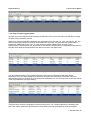
7.1 Supported models
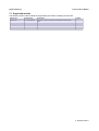
The following surface water models are supported by the triwaco modelling environment:
Modelcode
SOEBK-CF
Developed by
WL Delft/Deltares
Description
Hydraulic model for stationary and transient surface water
flow
Chapter
6
7 Surface water-3
Royal Haskoning
Triwaco User's Manual
7.2 The SOBEK-CF Tutorial: defining a Triwaco project
7.2.1 Introduction
There are several possibilities to get to know Triwaco. The most extensive information on the software
package can be found in the next chapters of the manual, that includes not only an explanation of how to run
the software, but also contains extensive background information of the different modules and supported
model codes. This information can also be accessed by the Help function.
This tutorial gives an introduction on how to set up and run a SOBEK-CF surface model in Triwaco. It is
meant for those who are familiar with SOBEK-CF modelling and wish to get a quick view of the normal
method to set up and to run a SOBEK-CF model, and the standard possibilities of Triwaco. A complete view
is obtained by using the manual.
It is strongly recommended that prior to starting this exercise one first reads through the previous
chapters which explain the general philosophy and handling of the Triwaco modelling environment.
Especially chapters 3, 4 and 5 is recommended to read first.
The model set up in this tutorial will be located in the directory C:\My Model\TutorialProject1\ All data referred
to in the text is available in the directory C:\My Models\TutorialData\. A resulting version of the model is
located in the directory C:\My Model\Tutorial\. So when things go wrong or you don't know what to do one can
always refer to this working model. Below an overview of the successive steps of building a model in Triwaco
is given.
6.2.1 Setting up a triwaco project
6.2.2 Setting up a surface water model
6.2.3 Setting up a discretisation dataset
6.2.4 Setting up a design dataset
6.2.5 Setting up a simulation dataset
6.2.6 Setting up a scenario dataset
Model building starts with the choice of boundaries and collection of data. This is done without the use of the
software, and will not be discussed here.
Triwaco works with a clear hierarchical data storage structure. The entry always is a project that can contain
several models. Every model consists of different connected datasets that contain different parameters.
7.2.2 The SOBEK-CF Tutorial
Regional – Local database construction
Data of the watersystem is often available in a regional database. The research area is a small part of the
regional database. We will show you how to use the regional database to set up a local SOBEK-CF model using
Triwaco.
7.2.3 Definition of a Triwaco Project
Now we show you the steps to take for making a SOBEK-CF model using Triwaco. We keep to the ‘main
route’; extra options are mentioned with the letter E and shown in italic. Important notices are indicated with NB.
Modelling with Triwaco always starts by defining a project. Choose 'File - New' if you want to set up a new
modelling project (otherwise choose 'File - Open' - and look for the location and name of your project). A wizard
will pop up which will guide you through setting up de project.
7 Surface water-4
Royal Haskoning
Triwaco User's Manual
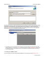
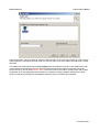
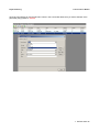
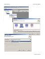
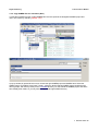
After finishing the wizard, you will see the start window of the modelling environment with the new project added
in the project list (see figure below). It gives all information of de modelling project, models, datasets and
parameters. For more information on the modelling environment see chapter 5. To add or remove windows go
to the menu 'View' in the top of the application-window. The modelling environment is fully customizable and
each window can be put at any location by simply drag and drop.
•
It is possible to use your favourite text editor, instead of the standard OpenSource editor that comes with
Triwaco, Notepad++. To do this go to 'Tools' in the task bar at the top. Select 'Edit Database'. This will open
the database in Access or other database editor. Go to Applications and change the path and location of
your favourite text-editor.
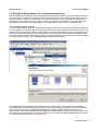
7.2.4 Setting up a SOBEK-CF model
If you want to add a new surface water model like SOBEK-CF to the project this is done by: 'Model - Add
7 Surface water-5
Royal Haskoning
Triwaco User's Manual
Model'. An existing model will already be listed in the project-window.
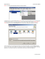
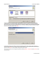
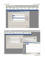
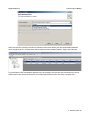
A wizard will pop up. In the first window select 'Next' to continue. In the second window one can choose the type
of model (see figure below). In our case we want to set up a surface water model. So select 'Surface water
model' and give it the name Tutorial-Regional (since we will start by setting up the regional model first).
In the next window one can select the model code to be used for the simulation. Currently Triwaco supports
only one surface water model, SOBEK-CF (a package for hydraulic modelling developed by Deltares / WLDelft
Hydraulics). In this tutorial we will set up a surface water model with the model code SOBEK-CF.
7 Surface water-6
Royal Haskoning
Triwaco User's Manual
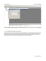
In the window there is also an option for selecting a parent model. This is used when setting up a sub-model or
scenario based on a previously created model. For now this option is not used. Select next and finish to create
the model.
The SOBEK-CF model with the name Tutorial-Regional is now added to the project. The SOBEK-CF model
can be opened in several ways. One can open it by double-clicking at its location in the project tree of the
project-window or one can select 'Model - Open' in the main menu. The model is currently empty and contains
no datasets. In the next paragraphs we will show how to add the necessary datasets to define the Tutorial
model. We will start by setting up a discretisation dataset where the calculation grid is defined.
7 Surface water-7
Royal Haskoning
Triwaco User's Manual
7.3 Setting up a discretisation dataset (regional)
The SOBEK-CF calculation grid is set up in the following steps :
1. definition of the discretisation dataset
2. definition of the model boundary
3. definition of the model attributes (grid parameters)
When the discretisation dataset, model boundary and model attributes have been defined the grid can be
generated (final step).
7.3.1 Step 1: Creating a discretisation dataset
The data for the generation of the network (calculation grid) is defined in the discretisation dataset. For the
discretisation of the Tutorial model we will use shape files for boundary, rivers and other model attributes (weirs,
laterals). All data used in this tutorial is available in the directory My Models\TutorialData\
First we add the discretisation dataset to the model by selecting 'Dataset - Add Dataset' from the main menu. A
pop up window will appear similar to that of adding a model. Again in the first window select 'Next' to continue.
In the second window one can choose the type of dataset. There are four types of datasets each with its own
characteristics and purpose:
● Discretisation: Defines the network or calculation grid (boundaries and model attributes)
● Design: Defines the conceptual model using GIS maps and tables.
● Simulation: Here is where the data from the conceptual model is linked to the calculation grid. The
model is now prepared to run with the modelcode.
● Scenario: Is similar to the simulation dataset. It is base upon the simulation dataset or another scenario
dataset. The dataset is created with parameters linked to the parent dataset. Only parameters that
need to be altered for that scenario have to be specified.
Each of these will be created in this tutorial with exception of the scenario dataset. In surface water modelling
the discretiosaint of a scenario is often different in comparsion to the discretisation of the reference model.
When defining a new discretisation one have to set up a new simulaiton dataset. So in surface water modelling
the simulation dataset is preferred in fovour of the scenario dataset. This will become clear in the rest of the
Tutorial. For now select 'Discretisation' and use the name Discr-regional for the dataset. Then select 'Next'.
7 Surface water-8
Royal Haskoning
Triwaco User's Manual
In the next window one may want to select a parent dataset. This is only of importance when a new grid is
created based on an existing discretisation dataset (like a sub-model or scenario). The nice thing about this
option is that a new model can be creating based on an existing conceptual model. We will show how this works
for a local study area in the XXX-part of this Tutortial. For now we are defining a regional discretisation dataset
and will not use a parent dataset; select 'Next'.
In the following window it is possible to change the appearing program options. These options describe for
example snapping distances for merging rivers and model attributes. In this Tutorial we will only use the default
options so select 'Next' to continue without changing the program options.
These program options can be changed at any time by selecting 'Dataset – Properties' and tab 'Options' for the
selected dataset.
7 Surface water-9
Royal Haskoning
Triwaco User's Manual
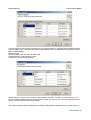
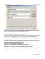
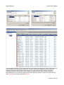
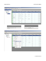
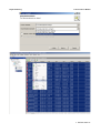
The next window is used to define parameters for the specified dataset. In the figure below the parameters for
model boundary, rivers, calculation grid density, fixed calculation points and lateral discharge points are shown:
BND = model boundary
REACH = rivers
CALCPNTDENS = density of the calculation grid
FIXEDCALCPNT = fixed calculation points
LATDISPNT = lateral discharge points
Usually there is no need to make changes to the specified parameters, so select 'Next' and after that 'Finish'.
Now the dataset is created and appears as part of the model. We will show you in the next paragraphs how to
remove, use and add parameters to the dataset.
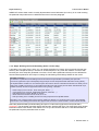
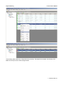
The screen shot below shows all parameters for defining a discretisation dataset that can be used to set up a
7 Surface water-10
Royal Haskoning
Triwaco User's Manual
SOBEK-CF surface water model. Currently all parameters have a bad status (red colour), in our case meaning
the parameter maps still have to be defined as we show in the next paragraph.
7.3.2 Step 2: Defining the model boundary (define a vector map)
A boundary or any map (rivers, weirs, etc.) can directly be defined in Triwaco from several file formats (see
text box), like a shape file set up in ArcView or ArcGIS, MapInfo or any other GIS software. For the model
boundary we use a shape file generated in ArcView. How to define parameters directly from the different file
formats will be explained in other steps of creating the calculation grid and design dataset for the model.
OpenGIS in Triwaco
For definition of parameter the modelling environment follows the specifications provided by the Open GIS
Consortium (OpenGIS or Open GeoSpatial) using the Open Source Geospatioal Data Abstraction Library (GDAL).
The implementation of GDAL into our software opens the world of all sorts of data file formats that can directly can be
read by the modelling environment. It can handle almost all known GIS formats (and the Dutch standards like Aquo,
INTWIS and IRIS). The list of supported formats is ever growing, a selection:
* Raster maps (over 64 formats ; Idrisi, ESRI grids, Erdas, …)
* Vector maps (over 16 format ; ESRI-shape, MapInfo, AutoCAD, …)
* Data bases such as Oracle, MySQL en Access;
* Other well known formats such as Excel, txt en csv.
* Data processing in the modelling environment using expressions and Spatial Queries
Data files in one of these formats can be used as model input without any conversion prior to use in the modelling
environment. The modelling environment also supports the conversion of model results to several data file formats
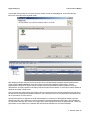
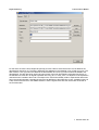
Select the parameter BND (model boundary) and open a context menu (right-click mouse) and select
'Properties'. The parameter properties window has two tabs, General and Input. The General tab gives general
information which is also shown in the dataset. For now you can leave this tab as it is. Note that the Status of
the parameters says the parameter does not exist.
7 Surface water-11
Royal Haskoning
Triwaco User's Manual
7 Surface water-12
Royal Haskoning
Triwaco User's Manual
Select the tab 'Input' and in the 'Type of Input' pull down menu choose 'Vector Map' for defining a shape-file.
Then use the 'Browse' button to select the boundary of the regional model (bound-regional.shp) in the
directory /My models/TutorialData/Modeldata/. After selecting the right shape-file it is obvious that the fields
'Filename' 'Datasource' and 'Layer' are automatically filled. The fields Filename and Datasource will now be
the same as shown in the figure. Select from the pull down menus of the fields 'Ids' and 'Values' the attribute
ID. Notice that this attribute is a field from the selected shape file bound-regional.shp. Leave the field 'Filter'
empty en click 'Close'.
7 Surface water-13
Royal Haskoning
Triwaco User's Manual
Note that the status bullet in the dataset for the boundary parameter is now green. You can check to see if the
files are stored in the right directory (the name of which must be the same as the name of the grid dataset).
Select and open the context menu for the parameter BND (Right hand mouse button) select 'Explore'. The
windows explorer is opened in the directory where the file should be located.
7.3.3 Step 3: definition of the model attributes (grid parameters)
As mentioned before we can define parameters directly from several file formats (see text box), like a shape file
set up in ArcView or ArcGIS, MapInfo or any other GIS software. In this Tutorial we will define all grid
parameters directly using a shape file which is provided in the directory My Models\TutorialData\Modeldata\.
There is no need for copying the files in this directory to the project. You could even leave it there for use in a
GIS project in the same time.
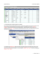
In the same manner as the definition of the model boundary we will define the location and source data of all
parameters. Use the figure and information below to define all parameters.
REACH: rivers (My Models\TutorialData\Geodata\rivers.shp)
WEIR: weirs (My Models\TutorialData\Geodata\weirs.shp)
PROFPNT: profile points (My Models\TutorialData\Geodata\profile-points.shp)
LATDISPNT: lateral discharge points (My Models\TutorialData\Modeldata\laterals.shp)
FIXEDCALCPNT: fixed calculation points (My Models\TutorialData\Modeldata\cal-points.shp)
BOUNDARYPNT: boundary points (My Models\TutorialData\Modeldata\bnd-points.shp)
The remaining parameters will not be used in this Tutorial model and should therefore be set on 'None' in the
input information. After defining all parameters the discretisation dataset is finished and should look like the
dataset in the figure below.
7 Surface water-14
Royal Haskoning
Triwaco User's Manual
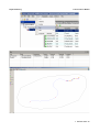
7.3.4 Generating the calculation grid (river network)
Now all data is entered (all status bullets are green), the grid can be generated. This is done in two steps. First
the grid input file is generated after which the grid is created. To generate the grid input file: 'Dataset Generate'. This will create the input file for the grid generator. Triwaco will show in the Jobs pane (if not
available do so by 'View - Jobs' the progress of generating the grid input file. In the Output pane the log of the
grind generator is shown.
To create the grid: 'Dataset - Run' Again information is provided in the Jobs and Output pane. When an error
occurs this is mentioned in the job pane or an error message may appear due to incorrect input. To find out
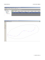
where it went wrong look into the log file. To view the log file: 'Dataset - View – Print'. To view the resulting grid:
'Dataset – View - Output'.
7 Surface water-15
Royal Haskoning
Triwaco User's Manual
7 Surface water-16
Royal Haskoning
Triwaco User's Manual
7.4 Setting up design dataset, the conceptual model set up
The conceptual model is defined in the Design data set. This data set contains the input parameters needed
to run the model. The data in this data set is independent from the grid and consists of data like vector maps
(ArcGIS, mapinfo), raster files, excel sheets, etc. The characteristics of each parameter are entered using
maps which may contain point values, polygons, lines or constants or a combination. The parameters may
also depend on each other using expressions. The default length and time units are meters and days.
7.4.1 Creating a Design data set
Go back a higher level to the level of the model Tutorial-Regional. This can be achieved by double clicking on
it in the project tree or by opening the context menu of the model Tutorial-Regional and selecting 'Open'. The
Design data set is created by: 'Dataset - Add Dataset' or selecting 'Add Dataset' from the context menu (right
click in the project-tree). A pop up window will appear the same as when we created the discretisation data
set. Again in the first window select next to continue. In the second window one can choose the type of dataset.
This time we select 'Design', name it Design1 (default name) and select 'Next'.
The following window that appears is for the definition of program options. In this window one can change
parameters which describe the properties of water and the environment (gravitational constant and density of
water). There is no reason to change these parameters so we will keep the default settings, click 'Next'.
In the following window all parameters that are added to the design dataset are shown. More experienced users
can add and remove parameters to specify the model. For now we want to add the default parameters so there
is no need to make changes, click 'Next' and 'Finish'.
7 Surface water-17
Royal Haskoning
Triwaco User's Manual
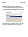
The design data set Design1 is now created and filled with the parameters (see figure above). Each SOBEK-CF
model is different and uses different kinds of river, boundary and structure definitions. Therefore different
TRIWACO parameters are needed to define the model. For this Tutorial model it is already know which
parameters should be used and which can be deleted. We will define them step-by-step in the following
paragrapahs but for now we need to delete all parameters. Select all, open the context menu (right click) and
select 'Delete' and in the pop up window 'Remove'.
7 Surface water-18
Royal Haskoning
Triwaco User's Manual
Within this design data set all parameter information is stored. In other words this data set is your meta
database for maps which are independent from the modelling grid. For definition of parameter the modelling
environment follows the specifications provided by the Open GIS Consortium (OpenGIS or Open GeoSpatial)
using the Open Source Geospatioal Data Abstraction Library (GDAL). The implementation of GDAL into our
software opens the world of all sorts of data file formats that can directly can be read by the modelling
environment. It can handle almost all known GIS formats (and the Dutch standards like Aquo, INTWIS and
IRIS). The list of supported formats is ever growing, a selection:
* Raster maps (over 64 formats ; Idrisi, ESRI grids, Erdas, …)
* Vector maps (over 16 format ; ESRI-shape, MapInfo, AutoCAD, …)
* Data bases such as Oracle, MySQL en Access;
* Other well known formats such as Excel, txt en csv.
* Data processing in the modelling environment using expressions and Spatial Queries
Data files in one of these formats can be used as model input without any conversion prior to use in the modelling
environment.
The design dataset is now empty and will be filled with parameters that define the Tutorial model. Parameters
in Triwaco can be divided in different types, accordingly to the type of structure, network-point or attribute in
SOBEK-CF.
The parameters for this Tutorial model can be divided in 5 types:
• River: parameters defining river properties (e.g. friction)
• Profile: parameters defining the dimensions of the river
• Boundary points: parameters defining the model boundary conditions
7 Surface water-19
Royal Haskoning
•
•
Triwaco User's Manual
Lateral discharge points: parameters defining lateral discharge properties
Weirs: parameters defining weir properties
It is important to notice that these 5 types are specifically for this Tutorial model. In a different model also other
structures can be used in the model for example culverts, controllers, orifices, etc. Successively other
parameters and parameter-types should be defined. All parameters that are selected in the parameter.xls
spreadsheet (program file). This spreadsheet should be used to understand the link between Triwaco and
SOBEK but may not be changed.
For the Tutorial model we will now show how and which parameters must be added to the design dataset. After
that we give a step-by-step description of the parameters definition.
7.4.2 Adding the parameters of the Tutorial model to the design dataset
The design dataset is empty so we will add the necessary parameters to the dataset. Make sure the Design1
dataset is activated and open the context window (right click) in the list window. Select the option 'Add
parameter' and a new window will appear. For now we will only fill in the name and type of all parameters and
define it later.
7 Surface water-20
Royal Haskoning
Triwaco User's Manual
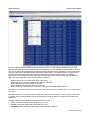
For the Tutorial model we will use a total of 19 parameters (see below):
bedfriction_MF
bedfriction_MTCPVALUE
bedfriction_MRCPVALUE
initialbranch_TY
initialbranch_LVLLVALUE
boundary_TY
boundary_FORM
boundary_ID
boundary_hqtables
profile_TY
profyz_NM
profyz_tables
weir_NM
weir_CL
weir_CW
weir_RT
lateralflbr_ID
lateralflbr_DCLT
lateralflbr_tables
type: river
type: river
type: river
type: river
type: river
type: boundary point
type: boundary point
type: boundary point
type: boundary point
type: profile
type: profile
type: profile
type: weir
type: weir
type: weir
type: weir
type: lateral
type: lateral
type: lateral
Add these parameters to the design dataset and make sure that he name and type of the parameter is defined.
7 Surface water-21
Royal Haskoning
Triwaco User's Manual
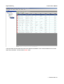
The parameters are automatically sorted per type (see figure below). It is possible to select only the parameters
defining a special type by clicking on the tab of for example 'River'. In the tab 'Parameters' all parameters of the
dataset are listed (like figure above). The tab 'Inherited' shows all listed parameters that are inherited from a
parent dataset. This dataset has been set up without a parent dataset so the list of inherited parameters is
empty.
7.4.3 Input of parameters Profile type
In this paragraph we define the parameters for the profile points. Three parameters have been added to the
dataset: profile_TY, profyz_NM and profyz_tables. These parameters describe the SOBEK-CF profile point with
a y-z cross section definition.
With the parameter prof_TY one can define the type of the cross section definition. This parameter can have
several value which represent different types of cross section definitions. In this case we use the value 10 for a
y-z cross section definition. So open the context menu (right click on the parameter profile_TY) and select the
tab 'Input' of the pop up window. Choose 'Constant' from the pull down menu of the field 'Type of Input' and fill in
10 in the 'Value' field.
7 Surface water-22
Royal Haskoning
Triwaco User's Manual
The parameter profyz_NM links a ID (name) to a y-z cross section definition. We have used a shape-file with
profile points in the discretisation dataset. Per profile point a ID has been defined and we will use the same ID's
for the cross section definition.
Open the context menu of the parameter profyz_NM (right click) and select the function 'Properties'. In the pop
up window choose the tab 'Input' and select the input type 'Vector map'. Next browse for the shape-file profpoints.shp in the directory XXX. The field for Filename, Datasource and Layer are automatically filled in. The
fields Ids and Values must link to the attribue ID_SOBEK in the shape-file. Now there is a link between the ID of
the profile point at the network (discritsation dataset) and the name (ID) of the cross section definition. Click on
'Close' to exit the input screen.
The final step in defining this parameter is to change its allocator. This should be done in the column 'Allocator'
of the parameter in the list window. Use the allocator 'Sobado' which is being used for shape-files and vector
maps.
7 Surface water-23
Royal Haskoning
Triwaco User's Manual
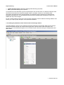
Now we have define the y-z cross section profile definition (see figures below). This is executed by the
parameter profyz_tables. We have the profile definitions of the four profiles of the Tutorial model listed in a
excel workbook (profile.xls) in directory XXX. Open the context menu (right click) of the parameter profyz_tables
and select 'Properties'. In the pop up window select the tab 'Input' and use the input type 'Table'. In the
appeared field 'Provider' select 'Microsoft Excel' because we have the profile definitions in an excel
spreadsheet. 'Connect' the right data source by browsing for the location (XXX)of the file profile.xls.
In the field 'Table' one can select the right worksheet. Use the pull down menu to choose the 'Tutorial'
worksheet. Now it is possible to look at the connected table by 'Show table' function. The table has three
columns ID_SOBEK, Y and Z. The first column is necessary for identifying the profile definition and link it to the
discretisation. Therefore select 'ID_SOBEK' from the pull down menu next to the Ids field. The Value field
cannot be defined using the pull down menu because we have to declare two columns, namely Y and Z.
Therefore fill in 'Y,Z' manually.
The final step for this parameter definition is to define its allocator. Allocation is translating parameter values
defined by maps or tables to a calculation grid and is carried out by allocators. Allocation is the spatial or temporal
interpolation or up/down scaling. Transformation to model parameter input is, usually, in the triwaco file format
(.ado or .adx). The reason for using this standard file format is that data can easily be exchanged between
models, all tools and processors can access it, automatic calibration tools will always work with any model, etc.
Also very important is that all transformed input data can be visualised with the built in viewers.
7 Surface water-24
Royal Haskoning
Triwaco User's Manual
Close the input window en use the Allocator column in the List window. Make sure you set the allocator of the
parameter profyz_tables to 'SobTab'.
7 Surface water-25
Royal Haskoning
Triwaco User's Manual
7 Surface water-26
Royal Haskoning
Triwaco User's Manual
7 Surface water-27
Royal Haskoning
Triwaco User's Manual
7 Surface water-28
Royal Haskoning
Triwaco User's Manual
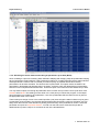
The parameters for the profile points are finished and your List window screen (tab profile points) should be look
like the figure below.
7 Surface water-29
Royal Haskoning
Triwaco User's Manual
7.4.4 Input of remaining parameters
We show you how to change the input settings of parameters. From now on we expect you are able to change
the input of the parameters yourself.
Weirs in the Tutorial model will be defined by four parameters: weir_NM, weir_CL, weir_CW and weir_RT. The
first three parameters should be linked to the shapefile XXX weirs.shp. The parameter weir_NM should be
linked to ID_SOBEK (ID of weir), weir_CL must link tot the attribue CRESTLEVEL and weir_CW to
CRESTWIDTH. The parameter weir_RT defines the flow direction and the value of 0 represents flow possible in
both directions. Make sure all parameters are define as shown in the figure below.
The parameters that define river properties represent friction of the riverbed and initial water depths.
Dimensions of the river have already been defined by the profile point parameters. Information about the
different parameters can be found in the parameter.xls spreadsheet. For now we only show you the input values
of the river parameters (see figure below).
The figure below shows the parameters for the boundary points. The Tutorial model has one boundary point
with a Q-h relation. Make sure all parameters in the boundary point tab are defined as shown in the figure.
7 Surface water-30
Royal Haskoning
Triwaco User's Manual
The lateral discharge points need three parameters in this Tutorial model. The discharge (time depended) is in
an excel spreadsheet.
7.4.5 Overview of all parameters Tutorial model
All parameters of the Tutorial model have been defined. The list window (tab Parameters) should be look like
the figure below. Check all settings of the parameters to make sure the design dataset is without errors.
7 Surface water-31
Royal Haskoning
Triwaco User's Manual
7 Surface water-32
Royal Haskoning
Triwaco User's Manual
7.5 Setting up a local model for the simulation
We have defined a regional discretisation set because database are often containing all information of a
catchment area. However we do not want to model a large catchment but just a small piece of the upstream
area. Therefore we have to define a second modelling level on which the local Tutorial model is based. First we
add a new Surface water model to the Tutorial-SOBEKCF project which we call Tutorial-Local.
7 Surface water-33
Royal Haskoning
Triwaco User's Manual
In de model code window we now select a parent model, namely Tutorial-Regional. The local model will
become a sub-model of the regional model.
After adding the model Tutorial-Local to the project tree a new discretisation dataset should be added to the
model (name it Discr-reference). Click 'Next' and in the Associated datasets window select 'TutorialRegional.Discr-Regional' as parent dataset. All parameters and its definitions will be inherited in the local
discretisation. All other properties and settings remain the same as the default, so click 'Next' until the dataset is
added to the model Tutorial-Local.
Now check the tabs 'Parameters' and 'Inherited' and one will notice that the inherited parameters are the same
as defined in the Reigonal discretisation dataset. In the 'Parameter' tab some new parameters are listed but we
do not need these, so remove them.
We want to make two changes in the local schematization in comparison to the Regional dataset, namely a
different boundary and a difference in weir discretisation. Both these parameters are listed in the inherited tab
so select them and open the context menu (right click). Select 'Modify' and check the parameter tab. These two
parameters are now listed in the parameter tab and should be defined for the local discretisation.
7 Surface water-34
Royal Haskoning
Triwaco User's Manual
7 Surface water-35
Royal Haskoning
Triwaco User's Manual
7 Surface water-36
Royal Haskoning
Triwaco User's Manual
The boundary will be defined by a shape file bound_local.shp. This shape file is located in the directory XXX.
Make sure the input screen is like the figure below.
7 Surface water-37
Royal Haskoning
Triwaco User's Manual
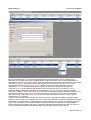
For the weirs we use the same shape-file (weir.shp) but use a filter to select which weir is to be added in the
discretisation and which not. The filter is defined by two attributes in the shapefile, mod_ref and mod_scen. The
filter is binair, a zero (0) means not added to the discretisation and a one (1) means it should be added to the
discretisation. The filter are being used in the input screen of the weir discretisation parameter (see figure). In
the field filter one must fill in an logical expression like mod_ref=1 or mod_scen=1. It depends on the expression
used which weir is added to the model. The shape of the Tutorial has already a filter to seperate the refernec3e
fromn the scenario situation. Normally the user have to add filters to the shape files. In fact, modelling is done in
a GIS environment and not in the SOBEK interface. See the figures below how the use the filter of the weir in
the Tutorial model.
7 Surface water-38
Royal Haskoning
Triwaco User's Manual
7 Surface water-39
Royal Haskoning
Triwaco User's Manual
7 Surface water-40
Royal Haskoning
Triwaco User's Manual
7.6 Setting up a simulation data set (reference situation)
Up to now the parameter values are stored independently of the calculation grid in tables and maps. The
advantage is that the grid can be changed without a change of the original input. The original input is linked
(allocated) to the grid in a separate data set, the simulation dataset. This is done only for the conceptual model
(design dataset).
7.6.1 Creating a simulation data set for the reference situation
Open the context menu for the sub model Tutorial-Local by right clicking on it in the project-tree and select 'Add
Dataset'.
A pop up window will appear the same as when we created the discretisation data set. Again in the first window
select next to continue. In the second window one can choose the type of dataset. Select 'Simulation' and
change the name to 'Sim-reference' and select 'Next'.
7 Surface water-41
Royal Haskoning
Triwaco User's Manual
The Simulation set combines the conceptual model (Design dataset) with a calculation grid of the local
schematization (Discretisation Local dataset) to create a local model (Simulation Local dataset) to run with the
specified model code. In the following window that appears the conceptual model (Design dataset) is selected
as the Parent dataset as well as the calculation grid of the reference discretisaton (Discr-reference dataset) as
the Discretisation dataset. Note that this means you can easily create an alternative grid and create a new
simulation dataset (thus a model) based upon the same conceptual model and visa versa.
•
Note that the datasets are defined as [Model name].[Dataset name], so here for the Parent Dataset
Tutorial-Regional.Design1.
Select next and find yourself in the same properties window when defining the design dataset. Leave everything
as it is. All information was inherited from the Design dataset. Select the 'Next' button and 'Finish' the dataset
wizard.
You are now back in the list of datasets in the model Tutorial-Local. Note that the dataset Simulation has a red
status indicator. Open the dataset Sim-reference. You will automatically will be directed in the Inherited tab.
Since the parameters are shown in a a different font (italic) than what you have seen before. The reason for
this is that it is immediately clear that you are dealing with inherited parameters. Also notice that all status
indicators are red which means they either need to be updated or allocation is not carried out yet.
7 Surface water-42
Royal Haskoning
Triwaco User's Manual
In the parameter tab new parameters have been added to the dataset. For the Tutorial model we do not need
these new parameters, so select all and 'Delete' them.
7 Surface water-43
Royal Haskoning
Triwaco User's Manual
7.6.2 Allocating the entire dataset and making all parameters up-to-date (Build)
Since modelling is a process of entering data, calibration adapting and changing maps and parameters keeping
track of all changes made is difficult. Triwaco already provides a lot of useful information via the status indicator
and dependencies. However with a lot of data you want as quickly as possible allocate all necessary
parameters to do another simulation. For this there is the option 'Build'. This option checks the status of all
parameters in the dataset and allocates them if necessary. It will also check the dependencies of parameters
and will in order of dependencies allocate them. So with one push of the button the entire dataset is up to date.
You may test this option even though all parameters at the moment are up to date. From the pull down menu
'Dataset' select 'Build'. The building process starts. In the Jobs pane you will see the progress. In the Output
pane information is provided for each parameter. If one of the parameters fails the reason for this is given,so
the appropriate action can be taken.
There is always a change of error in the model input files (.ado) even though the status indicator may be green.
It is therefore recommended to check all the allocated data (adore files) before running a simulation. One can
easily check the outcome of the allocation by looking at the summary of the parameter in Triwaco. Select the
parameter and open the 'Properties Window'. You will now see that next to General and Input tab an
additional tab is present, Output. Go to this tab to look at the allocated data.
7 Surface water-44
Royal Haskoning
Triwaco User's Manual
Additionally it is important to check the model within the SOBEK interface with the tools 'Validate network' and
'Check Flow model'. This is possible when the SOBEK-files have been copied in the designated case (after
executed 'Run' ; see paragraph XXX).
7.6.3 Generating the SOBEK-CF model-files (Generate)
When all parameters are allocated to the calculation grid and checked, the model is ready for the first simulation
run. The first thing that has to be done is to convert all parameters now in the standard Triwaco file format into
modelinput files for the model code as well as creating other input files to run the simulation with the specified
modelcode, in this case SOBEK-CF.
In the Simulation dataset select 'Dataset - Generate', which creates the input files for the SOBEK-CF model
code, based on the parameters defined in the dataset.
7 Surface water-45
Royal Haskoning
Triwaco User's Manual
7.6.4 Copy SOBEK-files for simulation (Run)
To start the simulation first the created SOBEK-files must be copied to the designated SOBEK project and
case. This is done by selecting 'Dataset - Run'.
A pop up window is opened where one can choose the right SOBEK-project and SOBEK-case. Select the
SOBEK-project TUTORIAL.lit and case Tutorial – reference. Notice that this SOBEK project should exist (as
dummy-project, with dummy cases) on the C:\SOBEK directory. For this tutorial the SOBEK-project and cases
have already been made, so you only have to copy it to the right SOBEK directory.
7 Surface water-46
Royal Haskoning
Triwaco User's Manual
7.7 Setting up a Scenario (scenario situation)
In most cases a surface water model or any other model is used to predict consequences of changes made to
the water system. These changes usually concern only a few model parameters. Scenario's in surface water
model result often in a change in network and therefore a new discretisation must be set up. Consequently,
when a new discretisation is set up, a new simulation dataset has to be defined. In TRIWACO it is not possible
to define a scenario dataset without defining a simulation dataset first. Therefore in surface water modellering
we choose to use a new discretisation dataset combined with a simulation dataset to define a scenario model.
In this paragraph we show how to add a new weir to the schematisation.
7.7.1 Creating a scenario dataset
Go back a higher level to the level of the model Tutorial-Local. This can be achieved by double clicking on it in
the project tree or by opening the context menu of the model Tutorial-Local and selecting 'Open'.
The new discretisation data set is created by: 'Dataset','Add Dataset'. A pop up window will appear the same as
when we created the other datasets. Again in the first window select next to continue. In the second window one
can choose the type of dataset. Select Discretisation and name it 'Discr-scenario' and select 'Next'.
In the following window that appears select Tutorial-Regional.Discr-regional as the Parent dataset.
7 Surface water-47
Royal Haskoning
Triwaco User's Manual
Select next and find yourself in the same properties window when defining the other discretisation datasets.
Leave everything as it is. All information was inherited from the Simulation dataset. Select next and finish.
Two parameters in the discretisation dataset have to be modified. The boundary has to be defined on a local
scale and the weirs need to be filtered for the scenario discretisation as we have seen in chapter XXX.
7 Surface water-48
Royal Haskoning
Triwaco User's Manual
7.7.2 The discretisation of the scenario model
Build' and 'Generate' the network and look at the the result ('Dataset' – View-output). Notice that a new weir has
been added to the network. Now we will create a new simulation dataset. It is not neccesary to create a design
dataset, because we can inherit all parameter definitions from the Regional design dataset. So, add a new
dataset to the project-tree. Choose a simulation dataset and name it 'Sim-scenario'.
'
7 Surface water-49
Royal Haskoning
Triwaco User's Manual
Select the 'Tutorial-Regional.Design1' as the Parent dataset and the 'Tutoral-Local.Discr-scenario' for the desired
scenario network. Select 'Next' a couple of times and the scenario simulation dataset will be added to the projecttree. Open the parameter window by double clicking it in the project tree. The necessary parameters have been
inherited from the design dataset (tab inherited) and again a large number of additional parameters have been
added to the dataset (tab parameter). These additional parameters should be deleted.
7 Surface water-50
Royal Haskoning
Triwaco User's Manual
7 Surface water-51
Royal Haskoning
Triwaco User's Manual
All parameters are ready because they have already been defined in the design dataset. Build and generate
the simulation dataset and the model is ready to run. To run the simulation choose 'Dataset','Run'. A
simulation window is opened showing the link to the SOBEK-model. Make sure that the SOBEK-model is
already on your hard disk. The SOBEK-model need to be ready up until 'schematisaion' (its colour should be
yellow). Select the right case 'Tutorial – scenario' and choose 'Run'. All files are being copied to the SOBEK
case and now you can open the model with the SOBEK interface and run the simulation.
7 Surface water-52
Royal Haskoning
Triwaco User's Manual
7 Surface water-53