Download Evaluating Spatial Normalization Methods for the Human Brain

Copyright 2005
Veronica Susanne Smith
Evaluating Spatial Normalization Methods
for the Human Brain
Veronica Susanne Smith
A thesis submitted in partial fulfillment
of the requirements for the degree of
Master of Science in Electrical Engineering
University of Washington
2005
Program Authorized to Offer Degree:
Department of Electrical Engineering
Abstract
Evaluating Spatial Normalization Methods for the Human Brain
Veronica Susanne Smith
Chair of the Supervisory Committee:
Professor Linda S. Shapiro
Department of Electrical Engineering
Department of Computer Science
Cortical stimulation mapping (CSM) studies have shown cortical locations for language function
are highly variable from one subject to the next. Because no two cortical surfaces are alike and
language is a higher order cognitive function, observed variability is attributable to a combination
of functional and anatomical variation. If individual variation can be normalized, patterns of
language organization may emerge that were heretofore hidden. In order to discover whether or
not such patterns exist, computer-aided spatial normalization is required. Because CSM data has
been collected on the cortical surface, we believe that a surface-based normalization method will
provide more accurate results than will a volume-based method. To investigate this hypothesis,
we evaluate a surface-based (Caret) and volume-based method (SPM2). For our application, the
"ideal" method would i) minimize variation as measured by spread reduction between cortical
language sites across subjects while also ii) preserving anatomical localization of sites.
Evaluation technique: Eleven MR image volumes and corresponding CSM site coordinates were
selected. Images were segmented to create left hemisphere surface reconstruction for each patient.
Individual surfaces were registered to the colin27 human brain atlas using each method.
Deformation parameters from each method were applied to CSM coordinates to obtain postnormalization coordinates in 2D space and 3D ICBM152 space. Accuracy metrics were
calculated i) as mean distance between language sites across subjects in both 2D and 3D space
and ii) by visual inspection of post-normalization site locations on a 2D map. Results: Globally,
we found no statistically significant difference between CARET (surface-based method) and
SPM2 (volume-based method) as measured by both spread reduction and anatomical localization.
Local analysis showed that more than twenty percent of total mapping errors were mapped
incorrectly by both methods. There was a statistically significant difference between Caret and
SPM2 mapping of type 2 errors.
i
TABLE OF CONTENTS
Page
List of Figures.................................................................................................................... ii
List of Tables.................................................................................................................... iv
Section 1: Introduction.......................................................................................................1
1.1 Registration of Medical Images ............................................................................1
1.2 Anatomical Variation ............................................................................................2
1.3 Functional Variation..............................................................................................4
1.4 Survey of Spatial Normalization Methods ...........................................................7
1.5 Cortical Stimulation Mapping and Visual Comparison Approach....................12
1.6 Hypothesis ...........................................................................................................16
Section 2: Survey of Evaluation Tools ............................................................................17
2.1 Surface Reconstruction .......................................................................................17
2.2 Surface Flattening................................................................................................20
2.3 Target Atlases......................................................................................................20
2.4 Spatial Normalization..........................................................................................25
Section 3: Methods...........................................................................................................28
Section 4: Results .............................................................................................................46
Section 5: Discussion .......................................................................................................58
Section 6: Future Work ....................................................................................................65
List of References.............................................................................................................67
Appendix A: Evaluation Protocol....................................................................................72
Appendix B: Resampling MRI ..................................................................................... 107
Appendix C: Creating a Stripped Coordinate File ....................................................... 108
Appendix D: norm_coord.m script ............................................................................... 109
Appendix E: merge_spm_foci.sh script........................................................................ 110
Appendix F: Spread Reduction Source Code............................................................... 111
Appendix G: Deformation Map File............................................................................. 123
ii
LIST OF FIGURES
Figure Number
Page
1. Anatomical Variation.....................................................................................................4
2. Functional Variation ......................................................................................................6
3. Intraoperative Photograph ...........................................................................................14
4. Skandha4 GUI Screenshot...........................................................................................15
5. Cerebral Neocortex Model ..........................................................................................17
6. SureFit Cortical Surface Reconstruction.....................................................................19
7. Visual Brain Mapper Screenshot.................................................................................29
8. Surface Reconstructions ..............................................................................................30
9. Flattening Template Cuts.............................................................................................33
10. 2D-3D Surface Relationships ....................................................................................33
11. Cortical Parcellation System .....................................................................................34
12. Normalization Process ...............................................................................................37
13. Core6 Landmarks-Inflated Surface ...........................................................................38
14. Core6 Landmarks-Spherical Surface ........................................................................38
15. Distance Metric..........................................................................................................41
16. P54 Language Sites....................................................................................................43
17. P117 Language Sites..................................................................................................43
18. Type 1 Error ...............................................................................................................44
19. Type 2 Error ...............................................................................................................45
20. Type 3 Error ...............................................................................................................45
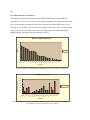
21. 2D Spread Reduction.................................................................................................47
22. 3D Spread Reduction.................................................................................................47
23. Caret Language Site Mapping...................................................................................49
24. SPM2 Language Site Mapping..................................................................................49
25. Number of CSM Sites per Parcel ..............................................................................50
26. Error Rate by CPS Parcel ..........................................................................................50
27. Error Type Analysis...................................................................................................51
iii
LIST OF FIGURES continued
Figure Number
Page
28. Refined 2D Spread Reduction ...................................................................................56
29. Refined 3D Spread Reduction ...................................................................................56
30. colin27 Atlas...............................................................................................................58
31. CPS Parcel Diagram...................................................................................................59
32. MSTG Shape Differences ..........................................................................................60
33. Sulcal Difference Map ...............................................................................................60
34. Language Site Mapping Summary ............................................................................64
iv
LIST OF TABLES
Table Number
Page
1. Central Sulcus Patterns ..................................................................................................3
2. Superior Temporal Sulcus Patterns ...............................................................................3
3. Subject Demographics .................................................................................................28
4. Statistically Significant Language Sites......................................................................36
5. Subject Surfaces and Volume Areas ...........................................................................42
6. Results Summary .........................................................................................................46
7. Caret Error Summary...................................................................................................48
8. SPM2 Error Summary .................................................................................................48
9. Same-Error-Type Mappings........................................................................................52
10. Unique Caret Errors ...................................................................................................53
11. Unique SPM2 Errors..................................................................................................54
12. Language Site Errors .................................................................................................55
13. Refined Spread Reduction Results............................................................................57
14. Correctly Mapped Language Sites ............................................................................57
v
ACKNOWLEDGMENTS
Thank you to Donna Hanlon and David Van Essen for their invaluable collaboration. A
special thank you to Richard Martin for being a great mentor and key contributor. To Dr.
George Ojemann, I offer sincere appreciation for your years of work in neuroscience and
suggesting this thesis topic. Thanks to Anthony Rossini and Thomas Lumley for
biostatistics consulting. Many thanks to Linda Shapiro, Jim Brinkley, David Corina and
the University of Washington Structural Informatics Group and Foundational Model of
Anatomy colleagues for your ongoing encouragement, feedback and support.
I am forever grateful for the encouragement, support and guidance I received from Amy
Feldman-Bawarshi and Frankye Jones from my beginning efforts to the attainment of this
degree. To Jennifer Girard, Ron Howell and Craig Duncan, I offer thanks for putting your
support into words and believing that I could change tracks successfully. Hank Hayes and
Abigail Van Slyck were also supportive mentors long before as well as during this
effort—thank you.
To Korin and Lois Haight, I offer my gratitude for being my most precious chosen
family. Chris Galvin was there, especially during the tough times, to help keep
perspective and light the way when I couldn’t see where I was going. To my mother, I
offer my thanks for being more than a survivor and showing me that I could make my
own way in the world. To my father, I offer my sincere appreciation for helping me excel
academically. To Natalie, I offer my deepest gratitude for making this opportunity
possible and for your unwavering love and support throughout this journey.
vi
DEDICATION
In honor of Frederick D. Hamrick III and Carolyn McGee Hamrick.
1
Section 1: Introduction
1.1 Registration of Medical Images
Within medical research and especially in neuroscience, medical images are used to investigate,
diagnose and treat disease processes as well as understand normal development. In neuroscience
research studies, it is often desirable to compare functional and structural images obtained from
the brains of patient cohorts. In addition, the amount of data produced using ever-improving
technology for generating medical images, increases exponentially with each successive
generation of imaging systems. It is essential, therefore, to have reliable, efficient, and accurate
methods for comparing and combining structural and functional brain images across subjects.
While the problem of comparing the brains of different individuals is an old one, the development
of computer-aided alignment, referred to as ‘intersubject registration’ or ‘spatial normalization’
has been substantial in the last decade.
We use the term ‘registration’ to mean determining the spatial alignment between images of the
same or different subjects, acquired with the same or different modalities, and also the
registration of images with a given coordinate system. The term ‘normalization’ is usually
restricted to the intersubject registration situation and is the term we will use in this paper. Spatial
normalization accuracy is a critical step to accurate quantitative analysis of the human cortex and
is the focus of this research.
Normalization is a form of alignment that involves two parts:
1) Positional normalization transformation: determination of a transformation that relates
the position of features in one image or coordinate space to the position of the
corresponding feature in another image or coordinate space. The symbol T will represent
this type of transformation.
2) Intensity normalization transformation: determination of a transformation that both
relates the position of corresponding features and enables us to compare the intensity
values at those positions. The symbol T will represent this type of transformation. Using
the language of geometry, we refer to the normalization transformation as a ‘mapping’
(Hill et al, 2000). The problem of accurately mapping data across subjects is confounded
by two factors: anatomical variation and functional variation.
2
1.2 Anatomical Variation
Notorious for the irregularity in depth and patterning of cerebral cortex convolutions, the human
brain structure varies notably from one person to the next. The human brain is an organ that is
exponentially more complex than other organs in the body. For example, the human lung has a
single primary function: respiration. On the other hand, brain function includes regulating all
bodily functions, language, the five senses and conscious thought, among others. When looking at
structural features like shape, surface and borders of the lung versus the brain, we again are
reminded of the brain’s complexity. In Gray’s Anatomy, it requires four times the amount of
visual and spatial description to characterize gross brain anatomy compared to that of the lung.
The cerebral cortex in particular reveals the brain’s structural complexity. The sulci (concavities)
and gyri (convexities) as viewed on the cortical surface serve as key landmarks to neuroscientists.
The Atlas of Cerebral Sulci by Ono et al. is a reference book documenting anatomical variation
of the cerebral sulci as a step toward describing and categorizing the highly varied structural
patterns of the cortical surface. Ono compared sulcal patterns of 25 autopsy human specimen
brains examined for anatomical variation and consistency in location, shape, size, dimensions and
relationship to parenchymal structures (Ono et al., 1990). Ono analyzed a total of 28 sulci: 15
large main sulci, six short main sulci and seven others. Six of the large main sulci are key
landmarks. They include central sulcus, lateral fissure (AKA Sylvan fissure), collateral sulcus,
callosal sulcus, calcarine sulcus and parieto-occipital sulcus. These sulci tend to have more stable
sulci patterns compared to other landmarks.
The central sulcus, located on the lateral surface of the frontal lobe is the most important and
constant landmark on the convexity of the brain. However, even this sulcus has notable variation
upon visual inspection of the shape of its inferior end. Ono found three different types of shapes
in the specimen brains. In the right hemisphere, 52% of the inferior ends were straight, 28% had a
Y and 20% had a T shape. In the left hemisphere, it was found that 80% of the inferior ends were
straight and 20% were T-shaped as outlined in table 1.
3
Table 1. Incidence rates of inferior end of central sulcus patterns as determined by Ono et al.
INFERIOR END SHAPE
LEFT HEMISPHERE
RIGHT HEMISPHERE
Straight
80 %
52 %
Y-shape
20 %
28 %
T-shape
0%
20 %
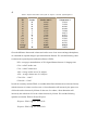
Table 2. Incidence rates of superior temporal sulcus patterns found in 25 human autopsy specimen brains.
PATTERN
LEFT HEMISPHERE
RIGHT HEMISPHERE
Continuous
28 %
36 %
Interrupted w/ 2 segments
32 %
48 %
Interrupted w/ 3 segments
16 %
16 %
Interrupted w/ 4 segments
24 %
0%
Greater variability was found on the lateral surface in the superior temporal sulcus. In table 2,
there are four patterns and the occurrence rate of those patterns. Notice how the patterns in this
case are much less predictable than the shape of the inferior end of the central sulcus.
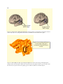
4
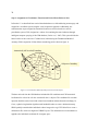
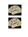
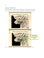
Figure 1. Left hemisphere of two different subject’s volume reconstructions. Red dashed line traces the
lateral fissure. Notice how the posterior end of this landmark, circled in red, differs across brains.
Ono’s study provides a broad analysis of cortical folding patterns. A localized example of
variation is demonstrated in figure 1. In this figure there are two volume reconstructions created
from Magnetic Resonance Images (MRI), using SKANDHA, a 3-D visualization software tool
(Prothero, 1995). The posterior tip of the lateral fissure is circled in red. The difference between
individual cortical folding patterns within the circled region is clear even to an untrained
observer. This degree of gross cortical structural variation between any two individuals makes it
difficult to accurately compare cohorts.
1.3 Functional Variation
The anatomy of the brain houses sensory, motor and cognitive functions. While language-related
functions were the first to be ascribed to a specific location in the human brain (Broca, 1861),
there is much more validation of and consensus around the anatomical location for sensory and
motor functions. A “classical model” of language organization, based on data from aphasic
patients with brain lesions, was popularized during the late 19th century and remains in common
use (Binder et al., 1997). In its most general form, this model defines a frontal, “expressive” area
for planning and executing speech and writing movements, named after Broca, and a posterior,
“receptive” area for analysis and identification of linguistic sensory stimuli, named after
Wernicke (Wernicke, 1874). Although many researchers generally accept this basic scheme, there
5
is not universal agreement on many of the details as well as whether or not Broca and
Wernicke’s areas are truly canonical (Binder et al., 1997). Ojemann et al. found in their electrical
stimulation mapping investigation of 117 epilepsy patients that the generally accepted model of
language localization in the cortex needed revision. The combination of discrete localization in
individual patients and substantial individual variability between patients found in the study
demonstrated that language cannot be reliably localized based on anatomic criteria alone.
(Ojemann et al., 1989)
Adding to the complexity of language function is that key findings in neuroscience and cognitive
science have shown that learning experiences change the physical microstructure of the brain,
which alter its functional organization. According to Bransford, “New synapses (junctions
through which information passes from one neuron to another) are added that would never have
existed without learning, and the wiring diagram of the brain continues to be reorganized
throughout one’s life.”(Bransford et al., 1999)
An example of experience determining how parcels of the brain are used can be found in the
brains of deaf people where some cortical areas typically used to process auditory information in
hearing people become organized to process visual information. There are also demonstrable
differences found across the brains of deaf people who use sign language and those who do not.
These structural and functional differences are presumably due to differing language experiences.
Another example of plasticity akin to the deaf reorganizing temporal cortex for visual processing
is blind subjects’ visual cortex reorganizing for language processing. Blind subjects asked to
generate verbs in response to heard nouns showed changes, as measured by fMRI, in the visual
cortex. Responses were greater and broader in early blind subjects than in late blind subjects
(Burton, 2003).
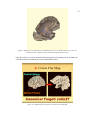
The functional data used in our research is cortical stimulation mapping for language localization
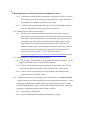
(described in Section 1.5). Figure 2 shows cortical stimulation sites identified as statistically
significant for naming errors are located in different areas of subjects’ left hemispheres. This
example of the same function being located in clearly different parts of the brain demonstrates the
marked individual functional variability in cortical locations essential for language production.
6
Figure 2. Functional Variation: surface reconstructions of four subject’s left hemispheres. The green
spheres represent sites that interrupted language production when electrically stimulated during awake
neurosurgery. Note how sites responsible for the same function appear on different areas of the cortex
depending on the subject.
7
1.4 Survey of Spatial Normalization Methods
Computer-aided spatial normalization is a widely used solution for relating the anatomy and
functionality of multiple brains in neuroscience and is a critical step in quantitative analysis of the
human brain cortex. It is not practical, nor desirable, to completely normalize the function and
structure of one brain to another. Rather, the goal of most researchers is to bring an individual’s
functional and structural data into a common visualization substrate with a set of common
coordinates. Having registered cortical structures, one can perform group or individual analyses
of structure and function to assess normal group differences in terms of age, gender, genetic
background, handedness, etc. (Ashburner et al., 2003; Davatzikos and Bryan, 2002; Mangin
et al., 2003; Thompson et al., 2001b). We can also better define disease-specific signatures and
detect individual cortical atrophy based on computational anatomy methods (May et al., 1999;
Thompson et al., 2001a; Toga and Thompson, 2003). Other applications for spatial normalization
methods include automatic cortical structural labeling and visualization (Le Goualher et al.,
1999), functional brain mapping (Toga and Mazziotta, 2000), and neurosurgical planning (Kikinis
et al., 1991). Given the wide array of intersubject registration applications, many image analysis
methodologies have been developed to address this need.
We define T as the spatial transformation (mapping) from source image to target image. We
define T as the transformation that maps both position and intensity. The first category of spatial
normalization methodology employs feature-based matching techniques. Normalization
algorithms that make use of geometrical features in images such as points, lines and/or surfaces,
determine the mapping of T (positional normalization transformation) by identifying features
such as sets of image points that correspond to the same physical entity visible in both images,
and calculating T for these features. Such algorithms iteratively determine T, and then infer T
(intensity normalization transformation) from T when the algorithm has converged. For the
purposes of this paper, we will refer to methods that use this type of algorithm as ‘surfacebased.’
The second category employs volumetric transformations involving intensity values. These
normalization algorithms iteratively determine the image transformation T that optimizes a voxel
similarity measure. We will refer to such methods as ‘volume-based’ (Hill et al., 2000).
8
Both surface-based and volume-based normalization methods may employ a ‘rigid body
transformation’, in other words there are six degrees of freedom (DOF) in the transformation:
three translations and three rotations. The key characteristic of a rigid body transformation is that
all distances are preserved. Rigid body transformations ignore tissue deformation and are widely
used in medical applications where the structures of interest are either bone or enclosed with bone
and are commonly used to register head and brain images. In the case of intersubject registration,
however, rigid body normalization does not provide enough DOF for adequate intersubject
registration. Some registration algorithms increase the DOF by allowing for anisotropic scaling,
giving nine DOF, and skews, giving 12 DOF. This type of transformation is referred to as affine
and can be described in matrix form. Also, an affine transformation preserves parallel lines. A
rigid-body transformation can be considered a special case of the affine, in which scaling values
are unity and skews equal zero (Hill et al., 2000).
While Hellier et al. did not find significant differences between an affine, a rigid and three nonaffine normalization methods when evaluating local measures based on matching of cortical sulci;
they did find that for global measures the quality of the registration is directly related to the
transformation’s DOF (Hellier et al., 2003). Collins and Evans compared rigid and non-affine
normalization methods. In this study, the rigid method revealed problems in maintaining accurate
global head shape and shape of internal structures like the ventricles as well as an error rate more
than 50% higher than the non-affine method (Collins and Evans, 1997).
Crivello’s comparison of one simple affine and three non-affine normalization methods including
i) fifth order polynomial warp, ii) discrete cosine basis functions and iii) a movement model
based on full multi-grid approaches support Hellier’s findings. When Crivello et al. used the four
methods to normalize 20 subjects’ MRIs and PET volumes to the Human Brain Atlas (HBA),
they found the full multi-grid approach, due to the large number of DOF, provided enhanced
alignment accuracy as compared to the other three methods. The fifth order polynomial warp and
discrete cosine basis function approaches exhibited similar performances for both gray and white
matter tissues and the affine approach had the lowest registration accuracy (Crivello et al., 2002).
9
Many authors refer to affine transformations as linear. This is not strictly true, as a linear map is
a special map L that satisfies: L(x + x ) = L( x ) + L( x ) where x, x and x =
any point in a mapping. The translational part of an affine transformation violates this. Thus, an
affine map is more correctly defined as the composition of linear transformations with
translations (Hill et al., 2000).
Grachev’s anatomically based assessment of the Talairach stereotaxic transformation (Talairach
and Tourneaux, 1988), a piece-wise affine algorithm, and a fifth-order polynomial transformation
(Woods et al., 1998) revealed that both methods located about 70% of anatomical landmarks with
an error of 3 mm or less. For landmark accuracy less than or equal to 1 mm, the Woods method
located about 40% of differences versus 23% for Talairach, again demonstrating the superior
accuracy of non-affine over affine spatial normalization methods (Grachev et al., 1998).
Davatzikos et al. compared two non-linear methods: SPM (Statistical Parametric Mapping), the
most widely used method for analysis of functional activation images, and STAR (Spatial
Transformation Algorithm for Registration). They found that STAR resulted in relatively better
registration (Davitzikos et al., 2001). SPM employs a volume-based approach that minimizes the
sum of the squared differences between the source image and target image while maximizing the
prior probability of the transformation. The maximum a posteriori solution is found iteratively:
the algorithm starts with an initial parameter estimate and searches from there. The SPM
algorithm stops when the weighted sum of square differences no longer decreases or after a finite
number of iterations (Salmond et al., 2002). The STAR algorithm differs from the SPM approach
in that it employs an elastic instead of a parametric transformation, thus it has thousands of DOF
compared to the relatively low DOF allowed for by SPM. Additionally, STAR applies surfacebased curvature matching along the cortex, thus incorporating shape information in the matching
mechanism. These differences were attributed to STAR’s improved registration (Davitzikos et al.,
2001).
SPM is one of many volume-based non-linear spatial normalization methods that have been
developed and used over the years. Others include deformable templates using large deformation
kinematics (Christenson et al., 1996), elastic deformation algorithm (Gee et al., 1993),
intersubject averaging and change-distribution analysis (Fox et al., 1988), unified framework for
10
boundary finding in a Bayesian formulation (Wang et al., 2000), statistical and geometric image
matching (Gee et al., 1994), automated image registration (AIR) (Woods et al., 1998), octree
spatial normalization (OSN) (Kochunuv et al., 1999), automatic non-linear image matching and
anatomical labeling (ANIMAL) (Collins and Evans, 1997), analysis for functional neuro images
(AFNI) (Cox, 1996) and maximization of mutual information (MMI) (Rueckert et al, 2001;
D’Agostino et al., 2002).
Surface-based non-linear spatial normalization methods include STAR, hybrid surface models
(Thompson and Toga, 1996), deformable surface algorithm (Davatzikos and Bryan, 1996),
generalized Dirichlet solution for mapping brain manifolds (Joshi et al., 1995), thin-plate splines
(Bookstein, 1989), unified non-rigid feature registration (Chui et al., 2003), computerized
anatomical reconstruction and editing tool kit (Caret) (Van Essen et al., 2001), Freesurfer (Fischl
et al., 1999), BrainVoyager (Kiebel, Goebel and Friston, 1999) iconic features (PASHA) (Cachier
et al., 2002) and active ribbons (Bizais, 1997).
There are also spatial normalization methods that incorporate aspects of both volumetric
transformations and surface-based matching. They include hybrid volumetric and surface warping
(Liu et al., 2004) and hierarchical attribute matching mechanism for elastic registration
(HAMMER) (Shen and Davatzikos, 2002), diffusing models (Thirion, 1998) and robust multigrid elastic registration (ROMEO) (Hellier and Barillot, 2003).
Researchers want to know, “What are reasonable expectations for each registration method?”
Crum has observed that there is a problem in the neuroimaging community in that we do not
usually know the quality of non-linear registration methods. We lack the necessary framework to
explicitly estimate and localize error for non-linear registration tools. He argues that as research
studies become more sophisticated, it is increasingly important to understand and measure the
degree, regional variation and confidence in the correspondences established by any given
registration. The solution lies in measuring quality at all stages of a non-linear registration task.
We must prescribe success criterion, quantify i) technical image quality, ii) relationship quality
between underlying biology and imaged features, and iii) registration quality (Crum et al., 2003).
Hill concurs that it is desirable to determine both the expected accuracy of a technique and also
the degree of accuracy obtained for any given set of data (Hill et al., 2001).
11
Like Hellier and Crivello, we wanted to evaluate the differences between spatial normalization
procedures by testing them on a given neuroimaging data set to determine which method should
be chosen for analysis (Hellier et al., 2003; Crivello et al., 2002). Other studies comparing
normalization methods in the literature include (Fischl et al., 1997; Gee et al., 1997; Grachev et
al., 1999; Minoshima et al., 1994; Roland et al., 1997; Senda et al., 1998; Sugiura
et al., 1999). Currently, the Neuroimaging Visualization and Data Analysis lab (NeuroVia) at the
University of Minnesota is conducting an evaluation of several spatial normalization methods
including AIR, SPM, ANIMAL, HAMMER, PASHA, ROMEO and DEMONS
(http://www.neurovia.umn.edu/neurovia.html). These studies used a variety of evaluation metrics
including the dispersion metric of selected landmarks, differential characteristics, tissue
classification, spatial homogeneity of selected anatomical features such as major sulci, overlap
percentage of restricted volume of interest, cross-comparison of 3D probability maps and visual
assessment.
Given the data set collected from cortical stimulation mapping for language localization, we
wanted to know what would be the best spatial normalization method to use for intersubject
registration to a canonical brain atlas. Friston states that goodness of a spatial transformation can
be framed in terms of face validity (established by demonstrating the transformation does what it
is supposed to), construct validity (established by comparison of techniques), reliability and
computational efficiency. In this evaluation study, conducted as part of the University of
Washington Human Brain Project, we address construct validity by comparing a surface-based
and volume-based normalization method and establishing an expected accuracy measure for the
given data set. We also address face validity by visual assessment of functional transformation to
anatomical substrate. Computational efficiency, reliability and overall cost-benefit analysis are
also discussed.
12
1.5 Cortical Stimulation Mapping and the Visual Comparison Approach
Since language function has been shown to vary significantly across patients, the technique of
intraoperative stimulation mapping is used in order to plan for treatment of temporal tumor or
intractable epilepsy at the University of Washington. Devised by Penfield and Roberts,
stimulation mapping was based on the observation that applying a current to some cortical sites
blocked ongoing object naming, although no effect of stimulating these sites was reported by the
quiet patient. Based on this work, stimulation mapping for language localization became an
accepted part of resective surgical technique for epilepsy. Stimulation mapping is used for
localizing language function within a hemisphere after lateralization has been determined
preoperatively by the intracarotid amobarbital perfusion test. Our data set consists of 11 patients
who underwent surgery on the left, dominant hemisphere. In order to insure that cortical surface
sites without evoked naming errors could be resected with a low risk of postoperative language
deficit, stimulation mapping must indicate both where language function is located and where it is
not. The extent of the craniotomy is determined in part by this consideration, covering both the
areas of the proposed resection and also the likely language locations (Ojemann et al., 1989).
The patient is put under general anesthesia for the craniotomy. Prior to mapping, rolandic cortex
is identified by stimulation and the threshold for after discharge in the electrocorticogram (ECoG)
is established for the area of association cortex to be sampled with language mapping. Language
mapping is conducted with the largest current that does not evoke after discharges. Typically this
current is in the 1.5 to 10 mA range, measured between peaks of biphasic square-wave pulses
with a total duration of 2.5 msec (1.25 msec for each phase). This current is delivered from a
constant-current stimulator in four second trains at 60 Hz across 1-mm bipolar electrodes
separated by 5 mm. Sites for stimulation mapping are randomly selected to cover the exposed
cortical surface, including areas where language function is likely located as well as proposed
resection. Typically there are 10-20 stimulation sites per subject that are identified with sterile
numbered tags and recorded with a digital intraoperative photo (Ojemann et al., 1989).
13
Once the craniotomy is complete, local anesthesia is applied to the dura and scalp and the patient
is brought to an awakened state in preparation for stimulation mapping, typically three to four
hours after the operation has begun. The awakened patient is shown slides of line drawings of
familiar objects like planes, boats, trees, etc. The slides are projected at four-second intervals,
with the patient trained to name each one as it appears. This is an easy task, and there are
frequently no naming errors on slides presented in absence of stimulation. Out of the 117 subjects
included in the Ojemann study, the highest error rate without stimulation was 22%. While the
patient names the slides, sites identified by numbered tags are successively stimulated, with the
current applied as the slide appears and continuing until the appearance of the next slide. At least
one slide without stimulation separates each stimulation and no site is stimulated twice in
succession. Usually several slides intervene between each stimulation, and all sites are stimulated
once before any site is stimulated a second time. Three samples of stimulation effect are usually
obtained. Intraoperative manual scoring of errors and their relations to stimulation provides
immediate feedback to the neurosurgeon (Ojemann et al., 1989). If the stimulation of a site results
in a naming error at least two of the three times, the site is determined to be essential for language
function. These sites are considered essential for language function because i) resecting tissue
close to such areas usually results in postoperative aphasis ii) avoiding them by 1.5 to 2 cm
avoids such language deficits and iii) all aphasic syndromes include anomia (Modayur et al.,
1997). In addition, the patient’s responses and markers indicating when and where stimulation
occurred is recorded on audio tape and used to later check the results to determine if the sites that
were identified as essential for language function are statistically significant for naming errors as
determined by the subject’s responses with and without stimulation.
14
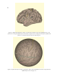
Figure 3. Surgical photograph taken during preparation for a left hemisphere
temporal lobe resection. The numbered tags identify sites that have been electrically stimulated, referred
to as cortical stimulation sites.
A visual comparison approach is used to transpose the location of the numbered tags as seen in
figure 3 to a 3D volume reconstruction of the cortical surface including veins and arteries.
The interactive mapping process is facilitated by the Skandha4 software package. As shown in
figure 4, the language mapping module graphic user interface (GUI) includes the intraoperative
photo, the MR volume data, a 3D rendered image of the brain and a palette of numbers. The
neuroanatomist expert determining the localization of the sites is blind to whether or not sites had
naming errors associated with them. All localization endeavors were given a confidence rating on
a scale from 1 to 5, where 1 is “not at all confident” and 5 is “very confident.” The ratings were
determined by amount and quality of images and descriptions. Using the blood vessels and
anatomical structure in the rendering as landmarks, the expert drags and drops the number that
corresponds to the number in the photo onto the rendered image. Once the site has been dropped,
a ‘pick’operation is performed in order to determine the closest surface facet to the site. The site
is assigned a 3D coordinate in MR ‘magnet space’ in which the center of the MR magnet is the
origin. This data is stored in a cortical stimulation mapping (CSM) database.
15
Figure 4. Skandha4 GUI used in the visual comparison approach
According to repeatability studies, any given mapping will typically fall within a distance of 5.1
mm of the true site location as measured by the mean of all the mappings (6 mappings included in
the study). Since the language site locations mapped during surgery are accurate to 1 cm, the
accuracy achieved using the visual comparison approach was deemed satisfactory (Modayur et
al., 1997). We found in a comparison of three independent mappings of two subject’s CSM sites
(n = 41 sites) that any given mapping could vary by an average of 7.5 mm, still within the 1 cm
margin of error for site location mapped during surgery.
16
1.6 Hypothesis
In this case study, we expected that reducing variation would better reveal functional patterns of
language production that exist in CSM language sites, which have been identified as statistically
significant for naming errors during neurosurgery. We believed that the problem of analyzing
CSM functional data across subjects can be solved using computer-aided spatial normalization.
As a result, we asked this key question: “What is the best spatial normalization method for
registering two or more brains such that the observed variation in the functional areas after
registration, as measured by cortical stimulation mapping (CSM), is the smallest?”
Because the data we used in our case study was collected on the cortical surface, we expected that
a surface-based normalization method, which relies on selected cortical surface landmarks, would
result in less variation between CSM language sites as compared to a volume-based
normalization method. For the same reason, we expected that the surface-based normalization
method would result in more accurate anatomical localization of CSM site locations.
17
Section 2: Survey of Evaluation Tools
Developing and implementing an evaluation technique for spatial normalization methods required
that we explicitly select tools for surface reconstruction, surface flattening, a target atlas and
spatial normalization.
2.1 Surface reconstruction tools
There have been many efforts to develop automated and semi-automated methods for
reconstructing the convolutions of the cerebral cortex. The tools surveyed are available outside
the laboratories in which they were developed.
Surface Reconstruction by Filtering and Intensity Transformations, called SureFit, was designed
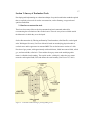
at the Washington University Van Essen lab and is based on an underlying physical model of
cerebral cortex and its appearance in structural MRI. The cerebral neocortex consists of a slablike sheet of gray matter, with approximately uniform thickness, folded into outward folds, called
gyri, and inward folds, called sulci. The transition from gray matter to the underlying white
matter is called the inner boundary. The cortical surface, called pial, is where the gray matter
meets the cerebrospinal fluid (CSF) and defines the outer boundary (Van Essen et al., 2001).
Figure 5. A schematic model showing a patch of folding cortex
18
SureFit generates a set of probabilistic maps for the location of gray matter, white matter, the
inner(gray-white) boundary, and the outer (pial) boundary as substrates for the segmentation
process using Gaussian intensity transformations (Van Essen et al., 2001). This generation
requires a complex set of filtering operations, intensity transformations, and other volumetric
operations applied to the image intensity data.
All filtering operations are applied to the 3D image volume. Inner and outer boundary maps are
particularly important, because they are combined to form a position map along the radial axis,
which runs from the inner to the outer boundary. The result is a position map along the radial axis
that is thresholded. The thresholding generates an initial cortical segmentation with a boundary
running approximately midway through the cortical sheet. The initial segmentation is used as the
substrate for generating an explicit surface reconstruction (Lorenson, 1987). SureFit currently
involves five major processing stages for segmentation as shown in figure 6.
19
Figure 6. Five steps for creating a surface reconstruction using SureFit. We completed the first five steps
for each subject’s left hemisphere. Instead of mapping fMRI data as the sixth step, we mapped CSM data.
Other tools considered include Freesurfer (Dale et al.,1999), mrGray-2.0 (Teo et al., 1998) and
BrainVoyager (Goebel et al., 1997). We selected SureFit primarily due to our past experience
with the tool and the desire to collaborate with the Van Essen Lab.
20
2.2 Surface flattening tools
The complex geometry of the human brain contains many folds and fissures making it impossible
to view the entire surface at once. Since most of the cortical activity occurs on these folds, it is
desirable to view the entire surface of the brain in a single view. This can be achieved using flat
maps of the cortical surface, which are essentially unwrapped cortical surfaces in a 2D plane (Van
Essen et al., 2001). Cortical flat maps also make it easier to see the depths and complete shape of
the sulci. Algorithms for creating flat maps do require cutting, compression and stretching of the
surface, causing some distortion. All cortical flattening methods aim to minimize geometric
distortion. We considered the following tools for creating cortical flat maps in this case study:
•
Computerized Anatomical Reconstruction and Editing Tool Kit (CARET)
(http://brainmap.wustl.edu/caret)
•
mrUnfold-5.0 (http://white.stanford.edu/~brian/mri/segmentUnfold.htm)
•
BrainVoyager (http://www.brainvoyager.de)
•
FreeSurfer (http://surfer.nmr.mgh.harvard.edu)
We selected Caret to flatten surfaces for two reasons. First, SureFit was selected for image
segmentation and is distributed and supported by the same lab as Caret. Thus, SureFit is designed
to interface seamlessly. In fact, work is underway to incorporate SureFit into the Caret software
suite. Secondly, since we selected Caret as one of the spatial normalization methods, using the
same software suite for flattening made for a streamlined evaluation protocol.
2.3 Target Atlases
Ideally a target atlas will not bias the final solution. An ideal template would consist of the
average of a large number of MR images that have been registered to within the accuracy of the
spatial normalization technique (Ashburner and Friston, 2000).
Talairach
Jean Talairach and Pierre Tournoux created the now famous book, Co-Planar Stereotaxic Atlas
of the Human Brain, in 1988. Talairach and Tournoux dissected and photographed a post
mortem brain of a 60 year-old female subject, creating a proportional coordinate system often
referred to as “Talairach space” for neurosurgical studies. This atlas was widely used in
international brain imaging studies and continues today to be the most widely used human brain
21
atlas. Talairach space consists of 12 rectangular regions of the target brain that are piecewise
affine transformed to corresponding regions in the template brain. Using this transformation, a
point in the target brain can be expressed in Talairach space coordinates, which allows for
comparison to similarly transformed points from other brains (Brinkley and Ross, 2002).
Today there is a database and data retrieval system named Talairach Daemon developed at the
University of Texas, San Antonio that performs the registration of target brains to the Talairach
template brain (http://ric.uthscsa.edu/projects/talairachdaemon.html). This system returns
anatomical labels using Brodmann area names for the cerebral cortex and other traditional,
feature-based terms when queried with a stereotaxic coordinate from an individual subject’s
brain. Thus, the Talairach Atlas provides a symbolic representation (textual) of the brain.
The entire Talairach brain has been anatomically labeled using a five-level, volume-based,
terminological hierarchy. Level One (“hemisphere”) has six components: left and right cerebrum;
left and right cerebellum; left and right brainstem. Level Two (“lobe”) divides each hemisphere
into lobes or lobe equivalents. In cerebrum and cerebellum, lobes are as traditionally defined. In
brainstem, three lobe-equivalents are defined: midbrain, pons and medulla. In both cerebrum and
cerebellum, brain areas lying deep in traditionally defined lobes are termed sub-lobar. Level
Three (“gyrus”) divides each lobe into gyri or gyral equivalents. Nuclear groups, such as
thalamus or striatum, are gyral equivalents. Level Four of the hierarchy is tissue type. Each gyrus
or gyral equivalent is segmented into grey matter, white matter and CSF. Level Five of the
hierarchy is cell population. Cerebral cortex is labeled by Brodmann area. Nuclear groups are
labeled by subnuclei. Cytoarchitectonic labels for cerebellar cortex and tract labels for white
matter are being developed but are not yet available.
The Talairach Daemon’s labels are stored as a volume array (1 mm isometric voxels) spanning
the extent of the brain in the Talairach 1988 atlas. This corresponds to approximately 500,000
voxels. Each voxel in this array contains a pointer to voxel-specific brain information. This
information is called a relation record and is managed as a linked list. A relation record can store
any information that is recorded using Talairach coordinates. To eliminate the need for storing
22
duplicate information in relation records, each record contains pointers to the information
rather than the information. This scheme offers the potential for extremely high speed access to
information within the relation records (Lancaster et al., 1997).
MNI305 and ICBM152
The Montreal Neurological Institute (MNI) wanted to define a template brain that was more
representative of the human population than the single brain used by Talairach and Tournoux.
They created a new template that was approximately matched to the Talairach brain via a twostep process. First, they used 241 normal MRI scans, and manually defined various landmarks
and the edges of the brain. Each brain was scaled to match the landmarks to equivalent positions
on the Talairach atlas. Second, a sample set of 305 normal MRI scans from right-handed male
(239) and female (66) individuals were normalized to the average template of the first 241 brains
using an automated 9 parameter affine transform. From this, MNI generated an average of the
305 brain scans. This atlas is known as the MNI305 atlas and was the first template created at
MNI. The current standard MNI template is named the ICBM152 because the International
Consortium for Brain Mapping adopted this atlas as their standard template. The ICBM152 atlas
was created from an average of 152 normal MRI scans that were normalized to the MNI305 using
a 9 parameter affine transform (Brett, 2003).
23
colin27 Atlas
A MNI lab member, Colin Holmes, underwent 27 MR brain scans. These scans were then
coregistered (registered to each other) and averaged to create a detailed MRI dataset of one brain.
The average of the 27 scans was then registered to the ICBM152 space to create what is called
“colin27,” also known as the Colin atlas. This template is used as a standard template in the MNI
brainweb simulator.
ICBM Probabilistic Atlases
Arthur Toga, Laboratory of Neuro Imaging (LONI) Director, and John Mazziotta, UCLA Brain
Mapping Center Director and principal investigator of ICBM, lead a team of researchers who
have created a variety of probabilistic atlases as they work to achieve the team’s ultimate goal of
a four-dimensional atlas and reference system that includes both macroscopic and microscopic
information on structure and function of the human brain in 7,000 persons between the ages of 18
and 90 years. As discussed, the fact that no single, unique physical representation for the human
brain is representative of the entire species, the variance must be encapsulated in an appropriate
framework.
Mazziotta and Toga have chosen a probabilistic framework in which intersubject variability is
captured as a multidimensional distribution. Accessing data from a probabilistic atlas will
produce a probability estimate of structures and function based on the distribution of samples
obtained. This frameworks also differ from frameworks like the ICBM152, which is an average
brain space. The average brain framework is created using a density-based approach. An atlas
using the density-based approach is an average space constructed from the average position,
orientation, scale and shear from all the individual subjects. It is, therefore, both an average of
intensities and of spatial positioning. Probabilistic atlases, like the ICBM Tissue Probabilistic
Atlas and Lobular Probabilistic Atlas proceed as follows:
•
Classify the desired components (tissue type or lobe type in these cases)
•
Average the separate components across the subjects to create probability fields for each
component that represent the likelihood of finding each component at a specified position for
an individual brain that has been linearly aligned to the atlas space (Toga and Mazziotta,
2000).
24
PALS-B12 Atlas
The Population-Average Landmark- and Surface-based atlas (PALS-B12) is a new electronic
atlas developed at the Washington University Van Essen Lab. Designed for brain-mapping
analysis, it is derived from the MRI volumes of 12 normal young adults and includes both
volume-based (MRI) and surface-based representations of the cortical shape. The population
average and individual subject representations were created using Caret, a surface-based method
of spatial normalization discussed in Section 2.4. The atlas includes sulcal depth maps as a
standard shape representation and depth-difference maps can be used to view differences between
individuals and across populations. The atlas also includes probabilistic representations of the
population average surface and volume (Van Essen, 2005).
This atlas was designed specifically to avoid the inevitable bias introduced when using a single
brain atlas as a target. A ‘multi-fiducial mapping’ method is introduced that maps volumeaveraged group functional data (e.g. fMRI) onto all 24 individual hemispheres in the atlas,
followed by spatial averaging across the individual maps, yielding a population-average surface
representation that shows the most likely regions of activation and the maximal extent of
plausible activation.
We selected the colin27 for primarily two reasons relating to the type of metrics we wished to
use. First, we wanted to measure pre-normalization and post-normalization distances between
language sites across brains both in 2D and 3D space. If we were to use an average brain atlas
(like ICBM152), the blurring that occurs from averaging multiple brains would distort the flat
map distances significantly after normalization, because the sulci would become significantly
shallower due to averaging as compared to the sulci in the individual flat maps. Second,
evaluation of anatomical localization using CPS required visualization of the data on a single
brain so as to determine if a site is indeed in the correct parcel. The blurring of sulci and gyri that
is a result of averaging individual MR images would make the evaluation very difficult if not
impossible. Given these constraints, we selected the colin27 atlas that we received from the
Laboratory of Neurological Imaging (LONI) at UCLA and registered it to MNI152 space using
SPM2.
25
2.4 Spatial normalization methods
We considered five spatial normalization software tools that are commonly used within and
outside the labs in which the tool was created. Other tools are discussed in Section 1.4. In
Section 6 we discuss possible future work of evaluating other methods to provide further insight
into how each method impacts results as well as the expected accuracy, efficiency and distinct
benefits of each method. We selected a method from each of the two categories discussed in
Section 1 as representative samples of each approach.
2.4.1 Surface-based anatomical normalization methods
Caret (http://brainmap.wustl.edu/caret)
Caret is a software tool developed by David Van Essen, Heather Drury and John Harwell at
Washington University. Options for surface-based transformation allow for the source to be
deformed to the target while constrained by explicitly designated landmarks, called ‘Core6’
landmarks. Core6 includes the fundi of the calcarine sulcus, central sulcus and lateral fissure; the
anterior half of the superior temporal gyrus (STG); and the medial wall cortical margin (split into
dorsal and ventral portions). These landmarks were selected on the basis of their consistency in
location and extent. Caret deforms flat maps or spherical maps. The spherical registration is more
accurate and uses an algorithm developed by Bakirciogli et al. (Van Essen et al., 2001). The basic
strategy is to draw landmarks as prescribed by the Core6 guidelines on the source map, then the
landmark contours are resampled to establish corresponding numbers of landmark points on each
source and target landmark contour. The landmarks are then used as constraints for the
deformation algorithm. The deformation entails using Laplacian differential operators constrained
to the tangent space of the sphere and basis functions that are expressed as spherical harmonics.
FreeSurfer (http://surfer.nmr.mgh.harvard.edu)
FreeSurfer is a software suite developed by Anders Dale and Bruce Fischl at Massachusetts
General Hospital’s Martinos Center for Biomedical Imaging and CorTechs Lab, Inc. Freesurfer
employs a spherical transformation to establish a uniform surface-based coordinate system.
Using this coordinate system, points on any of the surface representations for a given subject can
be indexed. Freesurfer employs a procedure that aligns a cortical hemisphere with an average
surface, based on an average convexity measure. By maximizing the correlation of the convexity
measure between the individual and the average, the procedure computes an optimal mapping to a
26
canonical target (Fischl et al., 1998). The FreeSurfer algorithm is very similar to Caret, except
that FreeSurfer normalization uses all sulci in maximizing correlation instead of a selected set of
landmarks, as is the case for the Caret algorithm. There is some evidence that the limited
landmark method may be superior, but more evidence is needed to exhaustively compare these
registration methods (Desai, 2004).
BrainVoyager (http://brainvoyager.de)
BrainVoyager software was developed by Rainier Goebel, Maastricht University, originally
introduced as a tool for analysis and visualization of functional and structural imaging data in
1998. It is now a commercial software package featuring cortex-based inter-subject normalization
based on gyral/sulcal patterns of individual brains as well as other functions listed previously
(Goebel, 2000).
2.4.2 Volume-based anatomical normalization methods
Analysis of Functional NeuroImages (AFNI)
(http://afni.nimh.nih.gov/afni/about/descripadfaad)
AFNI is a software environment for processing and displaying functional MRI data on an
anatomical substrate. It was designed and written at the Medical College of Wisconsin, primarily
by Robert Cox, now director of scientific and statistical computing core at the National Institute
of Mental Health. It is a free software package that uses a base unit of data storage called the ‘3D
dataset,’ which consists of one or more 3D arrays of voxel values with some control information
stored in a header file. AFNI’s spatial normalization feature requires the user to select various
markers first to align the anterior commisure and posterior commisure and a second set of
markers to define the bounding box of the subject’s brain. Then a 12 sub-volume piecewise linear
transformation to Talairach coordinates is performed for both anatomical and functional volumes
(Cox, 1996).
SPM2 (http://www.fil.ion.bpmf.ac.uk/spm/)
Karl Friston originally developed the software and associated theory for routine statistical
analysis of functional neuroimaging data. SPMclassic was the first version of the software suite
released in 1991 with the intent of promoting collaboration and a common analysis scheme across
27
laboratories. SPM has had five major revision releases since 1991. In this study, we consider the
most recent release, SPM2 ,released in 2003.
Spatial normalization using SPM2 is achieved by registering the individual MR images to the
same target image, by minimizing the residual sum of squared differences between them. The
first step in spatially normalizing each image involves matching the image by estimating the
optimum 12-parameter affine transformation (Ashburner et al., 1997). A Bayesian framework is
used, whereby the maximum a posteriori estimate of the spatial transformation is made using
prior knowledge of the normal variability of brain size. This step has been made more robust in
SPM2. Affine registering image A to match image B should now produce a result that is much
closer to the inverse of the affine transformation that matches image B to image A. A
regularization (a procedure for increasing stability) of the affine transformation has also changed.
The penalty for unlikely warps is now based on the matrix log of the affine transform matrix
being multivariate and normal.
The second step accounts for global nonlinear shape differences, which are modeled by a linear
combination of smooth spatial basis functions (Ashburner and Friston, 1999). The nonlinear
registration involves estimating the coefficients of the basis functions that minimize the residual
squared difference between the image and the template, while simultaneously maximizing the
smoothness of the deformations. This step has been improved in that the bending of energy of the
warps is used to regularize the procedure, rather than membrane energy. This model seems to
produce more realistic looking distortions. It is worth noting that this method of spatial
normalization corrects for global brain shape differences, but does not attempt to match other
cortical features (Ashburner and Friston, 2000).
28
Section 3: Methods
Subjects
The subjects were 11 patients (5 female, 6 male, age range 23-52 years) undergoing resection
treatment at the University of Washington Medical Center for chronic epilepsy (n = 11). Seven
patients were right handed. All cortical stimulation occurred in the subject’s left hemisphere,
which was identified as the subject’s language-dominant hemisphere in all subjects determined by
pre-surgery WADA testing (Corina et al., 2005). Subject demographics are summarized in
table 3.
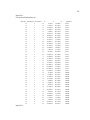
Table 3. Subjects’ gender, age, handedness and verbal IQ (VIQ)
BrainID
54
55
58
60
61
62
63
117
164
170
176
Gender
M
M
M
M
F
F
M
F
M
F
F
Age
25
30
23
38
35
24
42
41
42
52
41
Handed
ness
R
R
R
R
R
R
R
VIQ
107
83
86
72
91
92
125
97
94
75
82
Evaluation technique protocol
To test our hypothesis we developed a six-step evaluation protocol:
1: select MRI volumes
2: create surface reconstruction
3: create flat map
4: assign coordinates, function and cortical parcellation to each CSM site
5: apply spatial normalization to anatomical and functional data
6: evaluate methods using spread reduction and anatomical localization measures
29
Step 1: Select MRI volumes
Figure 7. Visual Brain Mapper screen shot. Upper left is a neurosurgery photo of the left temporal lobe
with sterilized labels identifying various cortical sites. To the right are coronal and axial slices from the
patient’s MRI taken prior to surgery. At lower left is the lateral left hemisphere view of a 3D brain model
including arteries and veins created from the patient’s MRI, venogram and arteriogram.
We selected 11 MR images from a University of Washington Structural Informatics Group
database of over 90 patients (CSM database). We screened the database images for left
hemisphere surgery, quality and lesions.
The first level of screening eliminated patients whose surgery was conducted on the right
hemisphere. By including only left hemispheres in this case study, we limit our scope to focus on
one major structural element of the brain. While left hemisphere surgeries are more common
than right hemisphere surgeries, future work would need to include analysis of the right
hemisphere as well as the left.
Image quality was the next level of screening. We determined quality by uniformity of voxel
intensity values, gray-white contrast within the image and artifacts, especially in the left temporal
30
lobe, our primary region of interest. Working with a SureFit expert, we were able to screen out
images that would require substantial manual error correction due to poor image quality. In one
instance (P62), non-uniformity of intensity was an issue. Using FSL’s fast algorithm
(http://www.fmrib.ox.ac.uk/fsl/fast) significantly improved the quality of the image, making it
possible to include the image in the data set. The final level of screening eliminated subjects with
large lesions.
Step 2: Create Surface Reconstruction
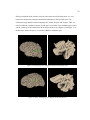
As discussed in Section 2.1, we selected SureFit to create surface reconstructions of the fourth
cortical layer of the left hemisphere of each subject’s brain. Figure 8 contains three of the 11
surface reconstructions segmented for this study and the surface reconstruction of the target atlas,
colin27.
Figure 8. Surface reconstructions of four left hemispheres created using SureFit
31
Prior to launching the automated segmentation process, the MRI volume was resampled to 1 mm
cubic voxels and cropped to included only the left hemisphere. The segmentation generated a
cortical surface reconstruction in approximately 1- 2 hours using a Dell Dimension dual 450Mhz
processor running Debian Linux.
Error detection and correction involved automatic correction and interactive editing. Topological
errors, called ‘handles,’ in the initial segmentation are typically attributable to noise, large blood
vessels, or regional inhomogeneities in the structural MRI volume, or a combination of these.
Errors were localized by inflating the initial surface reconstruction to a highly smoothed
ellipsoidal shape and using the orientation of surface normals to identify regions, called
‘crossovers,’ where the surface is folded over itself. Clusters of surface nodes associated with
crossovers were mapped from the surface reconstruction into corresponding voxel clusters in the
volume. The automated error correction process tested for different types of handles in the
vicinity of each location determined to have an error.
The localized patches used for these tests conformed to the shape of temporary segmentations that
are based on different threshold levels for the radial position map. If the trial patch reduced the
number of topological handles in the segmentation, as determined by an Euler count applied to
the volume (LeeT-C et al., 1994), it was accepted as a permanent correction and the process
moved on to the next error patch. (Van Essen, et al., 2001)
The automated error correction process sometimes failed, especially for handles that were notably
large or irregular. Such errors were corrected using interactive editing. For each handle that
remained after automatic error correction, the analyst used the object limits and 3D viewer to
identify the vicinity of each remaining handle. Voxels were then added or removed one at a time
or in small clusters using dilation and erosion steps within small masked regions. Error correction
was completed when no visible handles remained on the cortical surface reconstruction. The
quality of the SureFit-generated cortical segmentations was evaluated by visual inspection of
segmentation boundaries and of surface contours overlaid on the anatomical volume. This
assessment suggested that surfaces are generally accurate to within about 1 mm of their desired
trajectory (Van Essen, 2005).
32
Step 3: Create Flat Map
To aid in method evaluation, we created cortical flat maps using Caret as outlined in Section 2.2.
The SureFit specification file for the individual surface reconstruction was loaded into Caret. The
‘Flatten Surface’ functionality was selected. Then the six default cuts outlined on the medial
surface of the left hemisphere were inspected. The calcarine cut and medial wall cut were always
redrawn to match the specific structure of the individual surface. The remaining cuts (cingulate
cut, frontal cut, Sylvian cut, temporal cut) were redrawn, as needed, using the ‘Draw Border’
functionality. These cut lines were used to determine where the inflated surface was split in order
to achieve a cortical flat map. Figure 9 shows the template cut lines on the surface reconstruction,
and figure 10 shows how the surface reconstruction and flat map correlate.
33
Figure 9. Template cuts for flattening. The red dashed line traces the medial wall cut. Five other cuts
include calcarine, cingulate, frontal, lateral and temporal drawn in blue.
Once the cut lines were set, the automatic flattening took place. Flattening took 30-60 minutes on
a Dell Dimension 450 with dual processors running Debian Linux.
Figure 10. Relationship of 3D surface reconstruction to 2D flat map
34
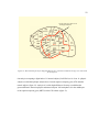
Step 4: Assignment of Coordinates, Function and Cortical Parcellation to Sites
In Section 1.5 we described how cortical stimulation data was collected during neurosurgery and
mapped to a coordinate system using the visual comparison approach. Additionally, the
neuroanatomist expert assigned an anatomical location to each site based on a cortical
parcellation system (CPS), designed as a scheme for examining the neural substrate through
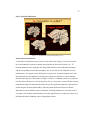
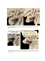
intelligent computer querying of the CSM database (Corina et al., 2005). This system divides the
lateral surface of the cortex into 37 subdivisions, labeled using the Foundational Model of
Anatomy (FMA) expansion of NeuroNames terminology and is shown in figure 11.
Anatomical (AKA sulcal) boundary
Subjective boundary
Figure 11. Cortical Parcellation System for lateral cortical surface
The data retrieved from the CSM database included the 3D coordinates and CPS anatomical
localization for each of the 198 sites recorded for the 11 subjects. The coordinate file was then
input into both the surface-based and volume-based methods and transformed accordingly. In
Caret, a spherical registration algorithm used landmark borders to create a deformation map.
SPM2 spatially normalized the individual volume image to the avg152T1 Minc file to create a
deformation file, which was aligned to ICBM152 space. The deformation for each method was
applied to the individual coordinate file in magnet space
35
coordinates, resulting in a normalized coordinate file. The result was a set of coordinate files
registered to the same reference space: ICBM152 space. These normalized coordinate files were
used to evaluate accuracy of each method based on spread reduction between sites and
preservation of anatomical localization (Step 6).
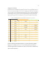
Of the 198 CSM sites, we were especially interested in the 21 sites identified as statistically
significant for naming errors (see table 4). Such sites have been found within and outside areas
classically considered language function regions. We believe that a hidden pattern of language
production exists that could be revealed with the help of spatial normalization. Statistical
significance was derived by analysis of the patients’ responses. Analysis included comparing the
patient’s pre-surgery test responses to the intraoperative test responses. To determine whether
naming disruption at a site determined by the neurosurgeon was an effect of stimulation or
attributable to the baseline naming error rate of the subject, a within-subject analysis of naming
errors was carried out. Fischer’s exact test (p < 0.05) was used to compare each subject’s baseline
performance, derived from the naming error rate in each control trial associated with the site,
regardless of target, and performance under stimulation at that site. This definition of baseline,
restricted to the controls associated with a certain site, was established to eliminate variation in
performance due to fatigue, inattention, and other physical factors experienced by the subject
during the procedure. The p value represents the reliability that an error was observed under
stimulation relative to the unstimulated baseline for each individual site (Corina et al., 2005).
36
Table 4. Summary of statistically significant language site anatomical localization
ID
P54
P54
P54
P54
P55
P58
P60
P60
P61
P61
P61
CSM # Location
20
PSTG
30
PSTG
35
PSTG
36
PSMG
41
MSTG
32
PMTG
29
MSTG
31
PMTG
25
MSTG
28
PMTG
29
PMTG
ID
P61
P62
P62
P63
P117
P117
P164
P164
P170
P176
CSM # Location
30
PSMG/AnG
33
OpIFG
35
TrIFG
25
MSTG
21
ASMG
33
PSMG
35
VPRG
40
ASMG
26
MSTG
28
MSTG
Generating pre-normalization coordinates that could be compared across subjects required
shifting the individual volume images into a common grid (i.e. standard voxel size, origin and
orientation). Without a common grid, we could not reasonably establish baseline distances
between language sites across subjects, which is necessary in order to measure spread reduction
after normalization (Step 6). Each subject’s volume has its own magnet center, and in some cases
the chin may be rotated up or down or slightly to the side. For pre-normalization coordinates, we
aligned the anterior commissure (AC) and posterior commissure (PC) using the AFNI software
package. This process resampled the volume to cubic 1 mm voxels and applied a rigid registration
to align the volumes to a common origin: the intersection of the superior edge and posterior
margin of the AC. AFNI also rotated the volume as needed so that its Y axis runs from the
inferior edge of the PC to the AC origin. Using AFNI, the AC superior edge and posterior margin,
the inferior edge of the PC and two mid-sagittal points were selected. AFNI then computed
transformation information that it stores in the volume .HEAD files. Then, the AFNI command
line utility, Vecwarp, was called to apply the transform to the individual coordinates, resulting in
pre-normalization AC-PC aligned coordinate files. These coordinate values were used to calculate
the pre-normalization distances (Euclidean distance) between language sites across subjects
(measure described in step 6).
37
Step 5: Spatial Normalization
Figure 12. Visualization of the normalization process
Surface-based normalization
To normalize the individual surface (source) to the colin27 atlas (target), we first need to select
the Core6 landmarks required to constrain the registration as discussed in Section 2.4.1. To
delineate landmarks traces along the sulci fundi, inflated surfaces of the individual hemisphere
and the corresponding colin27 atlas hemisphere were viewed side by side. Endpoints for each
landmark trace were drawn as prescribed by the Core6 protocol. Complete landmark traces were
then drawn between the endpoints on the flat map using the visualization of cortical folding to
determine the trajectory of the fundus (see figures 13 and 14). Landmark contours were projected
onto the surface and saved as a ‘border projection file’ in a ‘barycentric’ format. The file was then
mapped to the spherical standard surface that was used for registration. Spherical registration was
started using the ‘Deform Spherical Map’ function with the deformation selection ‘Deform
Individual to Atlas and Deform Atlas to Individual.’ Drawing landmarks for one subject took 1530 minutes. The automatic normalization process took approximately 15 minutes per subject on a
Dell Dimension dual 450Mhz processor running Debian Linux.
38
Figure 13. Inflated left hemisphere surface reconstruction with three of the Core6 landmark traces. The
yellow trace is along the fundus of the central sulcus, turquoise trace is along the lateral fissure fundus and
pink trace is along the tip of the superior temporal gyrus.
Figure 14. Spherical surface used for registration to atlas. Note the landmark traces that correspond to the
inflated surface traces in Figure 13.
39
Volume-based normalization
To normalize the source to the target using SPM2 we input the subject’s MR image in the form of
a Minc file with X increasing from patient left to right. No flipping was done during
normalization. With the exception of using the template bounding box and cubic 1 mm voxel
dimensions, the default spatial normalization settings were used. The selected template image was
a T1 Minc average volume of the MNI152 discussed in Section 2.3. Header and image warp files
were automatically written. Then, the ‘Deformation’ function, which writes header and image
deformation files using the normalized .mat file as input, was called. Next, the ‘Invert
Deformation’ function, which writes header and image inverse deformation files based on input
of the individual’s Minc volume, was called. The interactive normalization process took 15-20
minutes per subject on a Dell Dimension dual 450 Mhz processor running Debian Linux.
40
Step 6: Evaluation
Language Site Spread Reduction
In order to measure the change in distances between language sites across subjects prior to and
after applying selected spatial normalization methods; we needed to first measure these distances.
The following equations show how we measured distances between any two subjects. We
{
}
.
expanded these calculations for each of the 11 subjects and calculated B B ,B B ,...,B B
p 2 p 3
p 10
For subject p , the average distance between language sites in subject p and subject p prior to
1
B
B
=
normalization: p p
n*m
ni = 1 mj = 1 D( x pi , x
)
pj . The average distance
between language sites in subject p and subject p post-normalization:
1
B B =
p p
n*m
ni = 1 mj = 1 D( y pi , y
pj
)
where B = individual left hemisphere; n = number of language sites identified for subject p ; m =
number of language sites identified for subject p; D = Euclidian distance between points. X is a
variable representing site coordinates prior to normalization. Y is a variable representing site
coordinates after normalization. Euclidian distance between points was measured according to
D(a , b) =
this equation:
d
2
(a k bk )
k =1
where d = 2 or 3 depending on whether the coordinates are 2D or 3D.
41
Figure 15. Calculating average distance between language sites across two subjects, represented by the
orange and purple sites respectively
Figure 15 illustrates the distance calculation using three language sites of one subject (orange)
and two language sites from another subject (purple). Our distance measure used only the
distances between the orange and the purple sites.
We believe that the combination of anatomical and functional variation increases the distance
between language sites across patients. It follows, then, if anatomical variation is reduced, the
distance between language sites across brains will be reduced. Therefore, we expect that the
distance between language sites across patients, what we will refer to as ‘spread,’ will get smaller
after spatial normalization. The optimal method will maximize spread reduction. This hypothesis
assumes that the volume and surface areas of the source and target hemispheres are the same. As
we can see in Table 5, the mean surface and volume areas of the 11 subjects are less than the
target’s surface and volume areas.. To accommodate for this difference, we calculated the ratio of
the mean subject volume and surface area to the corresponding colin27 volume and surface area.
42
Table 5. Surface and volume areas of the 11 subjects’ an atlas’ left hemispheres
ID
54
55
58
60
61
62
63
117
164
170
176
average
colin27
Gender
M
M
M
M
F
F
M
F
M
F
F
M
Left Hem
Surface mm^2
86914
89032
99459
79299
85156
77723
75418
81613
88962
71963
67072
82055
107368
Left Hem
Volume mm^3
559616
512958
606962
466446
510960
448175
465153
498930
554765
423512
409783
496115
714773
Given the difference between the volume and surface areas of our source and target hemispheres,
we calculated an expected change in post-normalization distances. We used the following values
to estimate the expected post-normalization distance (EPoD):
PrD = average pre-normalization, AC-PC aligned distance between 21 language sites
CSA = colin27 surface area
CVA = colin27 volume area
ASA = average surface area of 11 subjects
AVA = average volume area of 11 subjects
CVA/AVA = 1.4407
CSA/ASA = 1.3085
In order to accurately estimate EPoD, we considered that linear distances do not increase linearly
with the increase of volume or surface areas. A linear dimension will increase by the square root
of M as the surface increases by M times. In the case of a volume, a linear dimension will
increase by the cubed root of N as the volume increases by N times. We used the following
equations to calculate EPoD in 2D and 3D space:
2D space: EPoD = CSA / ASA Pr D
3
3D space: EPoD = CVA / AVA Pr D
43
Having normalized for the increase in surface and volume area of the target atlas, we were
prepared to compare the actual post-normalization distances to the expected values. We
calculated average distance between language sites in both 2D space and 3D space. Thus, we
used two different coordinate systems: For 2D space we used the Caret coordinate space which
sets the ventral tip of the central sulcus as the origin (white cross in Figure 16 and Figure 17 on
the flat maps) and for 3D space, we used the ICBM152 coordinate space.
Figure 16. P54 language sites mapped in 3D(left) and 2D(right) space
Figure 17. P117 with language sites mapped in 3D and 2D space
44
Anatomical Localization
To measure how well anatomical normalization methods preserve anatomical location, we used
CPS as outlined in step 4. Following normalization using both methods, the neuroanatomist
expert viewed cortical flat maps including sulcal depth patterns and cortical sites via the Caret
GUI. The SPM2 normalization was viewed on the left side of the screen and the Caret data on
the right side of the screen. Each site number was identified via a mouse click. The
neuroanatomist identified the normalized location of each mapped site based on CPS. The author
recorded the post-normalization parcellations and compared them to the pre-normalization
parcellations, assigning a score and/or error type. A correct mapping received a score of 1. Error
types and scores were assigned as follows:
o
Type 1 Error: The site is located in an incorrect parcel across a subjective
boundary and receives a score of -0.25. Figure 18 illustrates this error type.
o
Type 2 Error: The site is located in the sulcus adjacent to the correct parcel and
receives a score of -0.5. Figure 19 illustrates this error type.
o
Type 3 Error: The site is located in the incorrect parcel across a sulcal boundary
and receives a score of -1. Figure 20 illustrates this error type.
Type 1 Error
Site should be
in MMTG
rG
VP
OpIFG
TrIFG
VPoG
A
Lateral Fissure
SM
G
PSMG
PSTG
PMTG
MSTG
ASTG
PolSTG
MMTG
AMTG
PolMTG
PITG
MITG
AITG
Figure 18. Example of Type 1 Error: Site is mis-mapped to a parcel across an subjective boundary as
delineated by a dashed line.
45
Figure 19. Example of Type 2 Error: P117 Pre-norm sulcal depth flat map with cortical sites on the left.
Post-norm flat map with normalized cortical sites on colin27 on the right. The language site (green) has
dropped into the sulcus
P164 CSM sites visualized
on P164 flat map
P164 normalized CSM sites
visualized on colin27 flat map
Figure 20. Example of Type 3 Error: P164 pre-normalized location of motor site (red) circled in blue is
mapped incorrectly as seen on the right. The post-normalization location has been moved across a sulcus
from VPrG to VPoG.
46
Section 4: Results
To determine which spatial normalization method would best transform cortical stimulation
mapping data to a target atlas, we measured both spread between statistically significant language
sites across subjects and preservation of anatomical localization as described in Section 3. Table 6
summarizes the results of the analysis for both measures. In 2D space, Caret reduced the average
distance between language sites across subjects 3 mm more than SPM2. Caret reduced the
average 3D distance between language sites across subjects .6 mm more than SPM2. Using the
jackknife estimate of variance, we did not show a statistically significant difference between the
surface-based and volume-based methods (Efron and Tibshirani, 1993).
Table 6. Summary of Results
Caret
SPM2
2D Spread Reduction
3D Spread Reduction
Localization Accuracy Rate
6.9 mm
3.9 mm
2.8 mm
2.2 mm
79.6%
78.0%
Anatomical localization accuracy rates as analyzed using a paired t test revealed a statistically
insignificant difference in overall accuracy between the surface-based method, resulting in 63
errors, and the volume-based method’s 62 errors when mapping a total of 198 sites. Qualitative
analysis of the error types provides more insight into some common and unique problems of
spatial normalization in this case study. Most notably, of the 125 total errors, 38 sites, 60% of
total errors, were incorrectly mapped by both methods. Also, a paired t test showed a statistically
significant difference in the type 2 errors mapped by both methods. While SPM2 normalization
resulted in only one type 2 error, Caret normalization resulted in 18 such errors.
47
Figure 21. 2D analysis of mean distance between 21 language sites across 11 subjects
Figure 22. 3D analysis of mean distance between 21 language sites across 11 subjects
48
Table 7. Caret Error Type Summary
ID
Type 1 Error Type 2 Error
54
0
4
55
2
2
58
1
1
60
1
2
61
4
2
62
1
1
63
2
1
117
0
2
164
0
1
170
4
2
176
3
0
Totals
18
18
Type 3 Error
3
4
2
5
1
2
7
1
2
0
0
27
Total Error
7
8
4
8
7
4
10
3
3
6
3
63
Table 8. SPM2 Error Type Summary
ID
Type 1 Error Type 2 Error
54
0
0
55
1
0
58
1
0
60
2
1
61
3
0
62
3
0
63
6
0
117
0
0
164
2
0
170
3
0
176
3
0
Totals
24
1
Type 3 Error
5
8
4
5
3
2
2
0
5
2
1
37
Total Error
5
9
5
8
6
5
8
0
7
5
4
62
49
Figure 23. Caret mapping of 21 language sites viewed on
colin27 inflated surface reconstruction
Figure 24. SPM2 mapping of 21 language sites viewed on
colin27 inflated surface reconstruction
50
Error Rate Analysis by CPS Parcel
The middle part of the superior temporal gyrus (MSTG) had the most assigned CSM sites
accounting for over 12% (24 of 198 sites) of all CSM sites mapped. The average error rate in this
parcel, as measured by averaging the sum of the Caret error rate and the SPM2 error rate, was
also high. 54.2% of MSTG sites were incorrectly mapped. Other parcels with 7 or more assigned
sites having an error rate of 50% or more were the posterior part of the supramarginal gyrus
(PSMG) and the ventral part of the precentral gyrus (VPrG).
Number of CSM Sites Per Parcel
30
25
CSM Sites
20
Num Sites
15
10
5
G
IF
TG
Tr
PI
G
TG
Pr
M
AI
rG
VP
oG
PM
TG
PS
TG
M
M
TG
AS
M
G
M
IT
G
O
pI
FG
PS
M
G
M
Po
G
PM
FG
AN
Po G
lS
TG
TG
VP
AS
TG
AM
M
ST
G
0
Parcel Name
Figure 25. Summary of 198 CSM sites included in this study broken down by CPS parcel.
Error Rate by CPS Parcel
Percentage of Errors
120.0%
100.0%
80.0%
60.0%
Avg Errors/Parcel
40.0%
20.0%
TG
AS
TG
VP
rG
VP
oG
PM
TG
PS
TG
M
M
T
AS G
M
G
M
IT
G
O
pI
FG
PS
M
G
M
Po
G
PM
FG
AN
Po G
lS
TG
M
Pr
G
AI
TG
PI
TG
Tr
IF
G
AM
M
ST
G
0.0%
Parcel Name
Figure 26. Summary of error rate by CPS parcel, descending left to right, from the parcel with the most
sites (MSTG) to the parcel with the least sites (TrIFG).
51
Error Type Analysis
A paired t test of all error types showed that the methods differed on average by less than a tenth
of an error per subject. The confidence interval (-1.2, 1.4) revealed that either method could be
better than the other by more than one error per subject.
Analysis of type 3 errors revealed the average difference for this error type was less than one
error per subject, Caret normalization could result in as much as two errors less per subject than
SPM2, while a SPM2 normalization could result in not more than 1 error less per subject than
Caret.
Type 2 error differences were statistically significant (p < .01). The confidence interval showed
that a SPM2 normalization could result in more than 2 errors less per subject than Caret, while a
Caret normalization could result in not more than 1 error less per subject than SPM2. Type 2
errors are discussed in Section 5.
Figure 27. Break down of same-type and unique mapping errors. Orange bar
indicates errors unique to Caret. Blue bar indicates errors unique to SPM2. Black
bar indicates errors shared by both methods.
52
Same-Error-Type Mappings
Figure 27 breaks down errors by type and whether the error was unique to one method or
common to both for a given site mapping. This analysis includes 105, or 84% of the 125 total
errors. Of the 38 common errors, 28 (20.7% of all errors) site mappings for both methods were
assigned the same error type (table 9). The remaining ten common errors were assigned different
error types, depending on the method. If the 28 same-error-type mappings had been correctly
mapped, 12 of the sites would have been located on the superior temporal gyrus (STG), four on
the angular gyrus (AnG) and four on the precentral gyrus (PrG), accounting for more than 71% of
the same error type mappings.
Table 9. Same-Error-Type Mappings: CSM sites mapped incorrectly by both methods and assigned the
same error types. Language sites are in bold with green background.
ID CSM #
Location
Score
P54
42
MSTG
-1
P54
37
PMFG
-1
P55
25
AMTG
-0.25
P55
33
AnG
-1
P55
41
MSTG
-1
P55
34
PSTG
-1
P58
9
VPrG
-1
P60
34
AnG
-1
P60
25
MITG
-0.5
P60
26
MSTG
-1
P60
29
MSTG
-1
P60
11
VPrG
-0.25
P61
31
AnG
-0.25
P61
21
ASTG
-1
P61
26
MMTG
-0.25
P61
30
PSMG/AnG -0.25
P62
28
MSTG
-1
P62
34
OpIFG
-0.25
P62
3
VPrG
-1
P63
23
ASTG
-1
P63
32
OpIFG
-0.25
P63
3
VPrG
-0.25
P164
23
ASTG
-1
P164
21
PolSTG
-1
P170
21
AMTG
-0.25
P170
23
ASTG
-0.25
P176
24
MMTG
-0.25
P176
27
MSTG
-0.25
CARET
SPM2
Error Correct Gyrus? Score Error Correct Gyrus?
3
no/MMTG
-1
3
no/MMTG
3
no/VPrG
-1
3
no/VPrG
1
MMTG
-0.25
1
MMTG
3
no/PSMG
-1
3
no/PSMG
3
no/MMTG
-1
3
no/MMTG
3
no/PMTG
1
3
no/PMTG
3
no/VPoG
-1
3
no/VPoG
3
no/PMTG
-1
3
no/PSTG
2
sulcus
-0.5
2
sulcus
3
no/MMTG
-1
3
no/MMTG
3
no/MMTG
-1
3
no/MMTG
1
no/VPoG
-0.25
1
no/VPoG
1
PMTG
-0.25
1
PMTG
3
no/AMTG
-1
3
no/AMTG
1
PMTG
-0.25
1
PMTG
1
PSMG
-0.25
1
PSMG
3
no/MMTG
-1
3
no/MMTG
1
VPrG
-0.25
1
VPrG
3
no/VPoG
-1
3
no/VPoG
3
no/MMTG
-1
3
no/MMTG
1
VPrG
-0.25
1
VPrG
1
VPoG
-0.25
1
VPoG
3
no/AMTG
-1
3
no/AMTG
3
no/AMTG
-1
3
no/AMTG
1
MMTG
-0.25
1
MMTG
1
PolSTG
-0.25
1
PolSTG
1
AMTG
-0.25
1
AMTG
1
ASTG
-0.25
1
ASTG
53
The same-error-type mappings, if scored using the protocol outlined in Section 3 (step 6),
represent a total deduction of 18.5 points. If these deductions were credited to the actual scores
for both methods, the resulting accuracy rate for both methods would increase by more than 9%
resulting in 88.89% accuracy for Caret and 87.37% accuracy for SPM2. Discussion on how to
improve mapping accuracy follows in Section 5.
Unique-Error-Type Mappings
Unique Caret errors (16) accounted for 25% of all Caret errors. Analysis of these errors reveals
that 31% of the errors should have been mapped to the middle part of the superior temporal gyrus
(MSTG). The other two parcels with the most common errors were the posterior part of the
superior temporal gyrus (PSTG), with 19% of errors, and the middle part of the middle temporal
gyrus (MMTG), with 13% of errors. Type 2 errors accounted for 56% of unique Caret errors.
Type 3 errors accounted for 38% of these errors, and there was a single type 1 error (6%).
Table 10. Summary of errors unique to the Caret spatial normalization method.
ID CSM #
P54
21
P54
43
P54
20
P54
30
P55
20
P58
25
P60
32
P60
10
P60
40
P61
34
P61
22
P62
27
P63
25
P63
20
P63
41
P63
22
P63
26
P63
31
P117
3
P117
33
P117
32
P164
25
P170
26
CARET
Location
MSTG
MSTG
PSTG
PSTG
ASTG
ASTG
PMTG
VPoG
PSTG
MPrG
ASTG
ASTG
MSTG
ASTG
AMTG
MSTG
MMTG
ASMG
MPoG
PSMG
PSMG
MMTG
MSTG
Score Error Correct Gyrus?
-0.5
2
sulcus
-0.5
2
sulcus
-0.5
2
sulcus
-1
3
NO/PMTG
-1
3
no/AMTG
1
3
no/AMTG
-0.5
2
sulcus
-1
3
no/ASTG
-1
3
no/PMTG
-0.25
1
VPrG
-0.5
2
sulcus
-0.5
2
sulcus
-0.5
2
sulcus
-1
3
no/AMTG
-1
3
no/MITG
-1
3
no/MMTG
-1
3
no/PSTG
-1
3
no/VPoG
-0.5
2
sulcus
-0.5
2
sulcus
-1
3
no/PMTG
-0.5
2
sulcus
-0.5
2
sulcus
54
Table 11. Summary of errors unique to the SPM2 spatial normalization method
ID CSM #
P54
24
P54
16
P55
37
P55
31
P58
31
P58
5
P58
23
P60
24
P60
30
P60
35
P61
27
P62
25
P62
5
P63
24
P63
27
P63
2
P63
40
P164
36
P164
29
P164
33
P164
7
P170
24
P176
25
SPM2
Location
VPrG
VPoG
AnG
ASMG
PSTG
VPrG
ASTG
AMTG
MITG
ASTG
MSTG
AMTG
VPrG
MITG
MITG
VPrG
ASTG
OpIFG
MSTG
PMTG
VPRG
AMTG
OpIFG
Score Error Correct Gyrus?
-1
3
no/VPoG
-1
3
no/VPrG
-1
3
no/PMTG
-1
3
no/PSMG
-0.25
1
PMTG
-1
3
no/VP0G
-1
3
no/VPoG
-0.25
1
no/MMTG
-1
3
no/MMTG
-1
3
no/VPoG
-1
3
no/PMTG
-0.25
1
MMTG
-0.25
1
OpIFG
-0.25
1
MMTG
-0.25
1
MMTG
-0.25
1
VPoG
-1
3
no/MMTG
-0.25
1
TrIFG
-1
3
no/MMTG
-1
3
no/PITG
-1
3
no/VPoG
-0.25
1
MMTG
-0.25
1
TrIFG
Seventeen errors were unique to the SPM2 spatial normalization method, representing over 27%
of all SPM2 errors. Error analysis reveals that the most common region to be erroneously mapped
was the ventral part of the precentral gyrus (VPrG), as more than 29% of unique errors should
have been mapped to this parcel. There are four other parcels that each account for more than
10% of SPM2 unique errors: middle part of the inferior temporal gyrus (MITG), anterior part of
the superior temporal gyrus (ASTG), middle part of the superior temporal gyrus (MSTG) and
opercular part of the inferior frontal gyrus (OpIFG). Type 3 errors accounted for 59% of the
unique errors with the remaining errors being type 1. There were no type 2 errors unique to the
SPM2 method.
55
Language Site Localization
Localization accuracy for language sites mapped by Caret was 72.62% versus SPM2 accuracy of
84.52%. Caret incorrectly mapped 9 (42.9%) of the 21 language sites. SPM2 incorrectly mapped
6 (28.6%). Again, we observed that the superior temporal gyrus (STG) was the most problematic
for both methods, with seven of the ten incorrectly mapped language sites being located on the
superior temporal gyrus (STG). Five language sites were incorrectly mapped by both methods.
Table 12. Summary of mapping by both methods of 21 language sites in 11 subjects.
CARET
ID
CSM #
P54
P54
P54
P54
P55
P58
P60
P60
P61
P61
P61
P61
P62
P62
P63
P117
P117
P164
P164
P170
P176
20
30
35
36
41
32
29
31
25
28
29
30
33
35
25
21
33
35
40
26
28
Location
Score
PSTG
-0.5
PSTG
-1
PSTG
1
PSMG
1
MSTG
-1
PMTG
1
MSTG
-1
PMTG
1
MSTG
-0.5
PMTG
1
PMTG
1
PSMG/AnG -0.25
OpIFG
1
TrIFG
1
MSTG
-0.5
ASMG
1
PSMG
-0.5
VPRG
1
ASMG
1
MSTG
-0.5
MSTG
1
Error
SPM2
Correct Gyrus? Score
2
3
sulcus
NO/PMTG
3
no/MMTG
3
no/MMTG
2
sulcus
1
PSMG
2
sulcus
2
sulcus
2
sulcus
1
1
1
1
-1
1
-1
1
-1
1
1
-0.25
1
1
1
-.25
1
1
1
1
1
Error
Correct Gyrus?
3
no/MMTG
3
no/MMTG
3
no/MMTG
1
PSMG
1
1
In order to refine the spread reduction analysis, we removed all incorrectly mapped
language sites, resulting in a data set of 11 sites. We then ran the spread reduction
calculation again with the revised data set (see table 14). The results are summarized in
figures 28 and 29 and table 13.
56
Figure 28. 2D analysis of mean distance between the 11 correctly mapped language sites
Figure 29. 3D analysis of mean distance between the 11 correctly mapped language sites
57
Table 13. Refined spread reduction results with the 11 correctly mapped language sites
n=11
Caret
SPM2
2D Spread Reduction
3D Spread Reduction
9.9 mm
4.8 mm
3.2 mm
1.3 mm
Table 14. Summary of 11 correctly mapped language sites
ID
CSM #
Location
P54
P54
P58
P60
P61
P61
P62
P62
P164
P164
P176
35
36
32
31
28
29
33
35
35
40
28
PSTG
PSMG
PMTG
PMTG
PMTG
PMTG
OpIFG
TrIFG
VPRG
ASMG
MSTG
The refined spread reduction analysis revealed an improvement for the Caret normalization
results and a slight degradation of the SPM2 normalization results. Caret reduced the spread
between sites by 5.1 mm more than SPM2 in 2D space. In 3d space, Caret reduced the spread by
1.9 mm more than SPM2. Using the jackknife estimate of variance method, we found that this
difference remained statistically insignificant. However, the difference in the means show that a
Caret mapping will, on average, be better than the SPM2 mapping by more than 5 mm in 2D
space and almost 2 mm in 3D space. Also, the confidence interval revealed that a Caret mapping
could be as much as 13 mm better than a SPM2 mapping in 2D space and more than 6 mm better
than a SPM2 mapping in 3D space. A power t test calculation was used to estimate the number of
subjects required to achieve a statistical significance of p <.05 and 80% power. We found that for
2D analysis we would need at least 55 subjects. For 3D analysis 120 or more subjects would be
required.
58
Section 5: Discussion
Anatomical Variation between Source and Target
The common mapping errors support what visual inspection of the structural surfaces of both the
source and target hemispheres revealed: locations of structural vagaries in both the colin27 and in
our subjects’ average surface reconstruction were where mapping error rates were 50% or greater
(figure 31).
The colin27 atlas structural regions were observed by a neuroanatomist to be atypical in the
ventral portion of the precentral gyrus (VPrG), supramarginal gyrus(SMG) and terminal
ascending segment of the lateral fissure (figure 30). These uncommon localized folding patterns
of the colin27 hemisphere help explain the average error rates of 50% or more in the VPrG and
PSMG, circled in figure 30.
VPrG
SMG
Figure 30. The colin27 atlas’ lateral left hemisphere surface reconstruction with areas of uncommon
cortical folding patterns circled in red.
59
Parcels in this area contain 175 of
198 mapped CSM sites
16.7%
57.1%
42.9%
50%
6.3%
54.2%
20%
45%
30.8%
9.4%
18.2%
35.7%
Figure 31. Most common parcels for mapped CSM sites are circled in red with the average error rate listed
for each parcel.
Our analysis comparing a digital atlas of 12 normal subjects (PALS-B12) to 10 of our 11 epileptic
subjects revealed that epileptic subjects have a broader superior temporal gyrus (STG) than the
normal subjects (figure 32). Analysis of a sulcal depth difference flat map, revealed that the
greatest difference between epileptic and normal subjects’ left hemispheres is in the middle part
of the superior temporal gyrus (MSTG) on the CPS scheme (figure 33).
60
average epileptic
MSTG shape
average normal
MSTG shape
Figure 32. Comparison of inflated left hemisphere average surface reconstruction of 10 epileptic subjects
in this study (left) to 12 young adult normal subjects included in the PALS-B12 atlas (right).
Region of most striking differences
in sulcal depth. This region
corresponds to the MSTG parcel
on CPS.
Figure 33. Sulcal difference map representing the differences between the average sulcal depth of 10
epileptic and 12 normal subjects. Dark areas represent where the epileptic subjects’ gyri are deeper and
the white areas represent where the epileptic gyri are shallower than the 12 normal subjects.
61
The colin27 atlas’ uncommon folding patterns of the supramarginal gyrus and lateral fissure are
documented by Ono in the Atlas of Cerebral Sulci. Four left terminal ascending segment patterns
were delineated. Upon inspection, the colin27 folding pattern most closely matched the pattern
illustrated in figure 15.9D in the Ono text. It is described as follows: “a descending terminal
portion which does not constitute the posterior transverse temporal sulcus.” This pattern occurred
in 4% of the 25 autopsy specimen brains examined for variations and consistencies in location,
shape, size dimensions and relationships to parenchymal structures (Ono et al., 1990). Two of the
remaining three patterns represented 88% of the folding patterns found in this region with the
final pattern representing 8% of the patterns found. This gyral pattern impacts the sulcal pattern
of the supramarginal gyrus (SMG), as SMG surrounds the posterior tip of the lateral fissure,
contributing to colin27 atlas’ unusual folding pattern in this parcel.
It is well known that anatomical variation between source and target can prove problematic for
accurate registration. This study supports previous findings that show we cannot expect to
completely normalize folding patterns across individuals. It also highlights the bias introduced by
a single brain atlas. In this study, we hypothesize that areas of important variability between
source and target are a key cause of at least 20% of the total anatomical localization errors.
Possible solutions to the problem of important anatomical variation between source and target
include creating a probabilistic atlas of epilepsy subjects, perhaps using the same 11 subjects.
This atlas would incorporate the average sulcal shape of the subjects, presumably resulting in
better anatomical alignment and more accurate normalization. Extrapolation of these findings to
the normal brain would require a transform of the functional data to a normal subject atlas. An
atlas of normal brains, like the PALS-B12 or ICBM atlases, would be a preferable target. What
currently prevents this technique from being implemented is the limited functionality available to
map CSM functional data to these atlases. There currently exists functionality to map fMRI data
to these atlases as fMRI is the most commonly mapped functional data. However, CSM site data
is relatively rare in the neuroscience community and therefore is not accommodated for as
broadly as is fMRI. Additionally, using a probabilistic atlas introduces a problem in reliably
measuring post-normalization surface distances that would need to be addressed and is discussed
in Section 6.
62
Type 2 Errors
A paired t test of type 2 errors did reveal a statistically significant difference (p < .01) in the
methods. SPM2 mappings resulted in only one type 2 error compared to 18 type 2 errors mapped
using Caret. The average difference between methods was 1.55 errors per subject. We believe
that this difference is attributable to the underlying differences in normalization approaches used
by the different methods. The SPM2 algorithm maximizes a voxel intensity match between
source and target. As a result, the volume-based method will very rarely end up with an alignment
resulting in a pre-normalized gyral location (i.e. CSM sites are always on the gyrus) being
relocated into a sulcus, where the voxel intensity is markedly less than the intensity found on a
gyrus. The surface-based method, however, maximizes alignment of a set of landmarks based on
cortical folding patterns without consideration for voxel intensity. If the selected landmarks vary
enough between the source and target, then the normalized sulci and gyri will be deformed in
ways that confound mapping of functional data to corresponding regions of the anatomical
substrate. The Core6 landmark protocol was designed to minimize this problem by selecting the
most stable landmarks and constraining the extent of each landmark to regions where it is
reasonable to expect good correspondence across nearly all subjects (Van Essen, 2005). Since
performing the spatial normalization for our 11 subjects (9/2004), there has been a clarification
on the starting point of the lateral fissure landmark border that we believe will impact the
normalization in the middle part of the superior temporal gyrus and sulcus (STS/STG), the region
where there is important variation between the subjects’ and colin27’s cortical folding patterns
and the region to which most errors were attributed. Specifically, redrawing the lateral fissure
landmark border for each of the 11 subjects according to the clarified guidelines is expected to
constrain the STS/STG more medial dorsally, which will tend to reduce differences summarized
in Figures 32 and 33. Given this landmark revision, we would expect to see a marked decrease in
type 2 errors as a result of Caret normalization.
Cost Benefit Analysis
Using SPM2 to normalize the CSM coordinates required notably less user input and time than
using Caret, because SPM2 does not require a surface reconstruction for normalization to the
target. To run SPM2 normalization, the only input required is a Minc file of the MRI and a text
file including the original CSM coordinates. With this input, an experienced analyst can generate
63
the normalized cortical site coordinates in approximately 20 minutes or less. Using the surfacebase method, the input required includes a surface reconstruction, which requires a total of 1 hour
of interactive processing and 1-2 hours for segmentation. Once the surface reconstruction is
complete, the input for the surface-based method is the surface reconstruction and the coordinate
file. At this point, the automatic surface-based normalization takes about the same time as the
volume-based method: 15-20 minutes. If a normalized set of deformed CSM coordinates is the
only desired result from the anatomical normalization process, then the volume-based method is
less expensive and will provide an overall accuracy of approximately 78%. If visualization of the
results is desirable, then the surface-based method is superior to the volume-based method, which
is not designed for visualization of cortical site data. (SPM2 is used to visualized fMRI, however)
Without creating the surface reconstructions required for Caret, we would not have been able to
localize the notable variation between the subjects’ average surface and the target atlas in the
superior temporal gyrus or assess the bias introduced by the colin27 atlas’ atypical folding
patterns in the supramarginal gyrus and ventral part of the central sulcus. Additionally, the
visualization of the CSM mappings was critical to assessing method accuracy. Knowledge of the
accuracy of a given method is key to researchers choosing the best spatial normalization method
for their work.
The challenge of validating the volume-based method is discussed by Crum. He advocates for
registration tools that monitor their own performance and estimate correspondence error with
minimal intervention (Crum et al., 2003). We also support this type of functionality in spatial
normalization tools like Caret and SPM2. We demonstrated that the surface-based method allows
for more quantitative and qualitative assessment of tool performance than does the volume-based
method. This evaluation led to a deeper understanding of the limitations and advantages of each
method and provides a frame work that can be used, with modification, to determine spatial
normalization accuracy.
64
Language Localization Patterns
Figure 34 illustrates the cortical parcellation of 16 language sites as mapped by Caret and SPM2.
The five sites that were incorrectly mapped by both methods are excluded from this illustration.
Most common
parcels for language
sites highlighted in
green
Figure 34. Mappings of 16 language sites on the colin27 atlas with incorrect mappings circled in red.
65
Section 6: Future Work
Possible future work includes repeating the study, with a larger sample, using a probabilistic atlas
as the target, repeating the study using subject fMRI data instead of CSM site data, repeating the
Caret normalization of the current data set using modified landmark guidelines, incorporating
standard metrics into the evaluation protocol and repeating the study to compare Freesurfer,
BrainVoyager, AFNI, a hybrid registration algorithm and a MMI registration algorithm.
As discussed in Section 2.3, we would have preferred a population atlas as our target, like
PALS- 12B, because of the inherent structural bias introduced to normalization by any single
brain atlas. We expect that using a probabilistic atlas would significantly increase the anatomical
preservation accuracy of both methods. The problem of multi-fiducial mapping for CSM sites
could be circumvented by using individual deformed files to assign nodes to the CSM sites that
could then be viewed on a variety of substrates (e.g. colin27, PALS 12B, average subject
surfaces, etc.) With this type of visualization, we would create a ‘zone’ for each site that would
capture the average location of a given CSM site across subjects and likelihood as to where any
given site would fall within this zone. This approach would require modification to the spread
reduction calculation. To achieve statistical significance of p < .05and 80% power, we would
want to increase the number of subjects to at least 60 and preferably 100 or more.
Functional MRI data has been collected on many of the subjects in the CSM database. It would be
interesting to repeat this study, replacing the CSM data with the fMRI data, using multi-fiducial
mapping to view results. This study could serve as validation of both methods and further
contribute to an understanding of what accuracy can be expected when using each method.
We plan to repeat the surface-based method using the recently modified Core6 landmarks to
analyze the impact this change will have on the mapping results. We expect that this modification
will increase the accuracy of the surface-based method by 5-10%.
66
The metrics used in this study were designed based on the nature of the CSM functional data. It
would be valuable to evaluate the methods using metrics used to validate other methods. For
example dispersion metric of selected landmarks, overlap percentage and cross-comparison of
maps would be interesting measures to use to further evaluate surface-based and volume-based
methods.
Repeating the study using FreeSurfer, BrainVoyager and AFNI would provide more insight into
how different surface-based and volume-based methods compare to each other and across
categories. Evaluating hybrid spatial normalization methods like HAMMER and ROMEO, which
employ feature-based and intensity matching techniques, would also be valuable. Additionally, a
relatively recent development is the use of maximization of mutual information (MMI)
registration. MMI is a strategy that has proved extremely successful at automatically computing
the registration of 3-D multimodal medical images of various organs from the image content.
Mutual Information (MI) is a basic concept from information theory, that is applied in the context
of image registration to measure the amount of information that one image contains about the
other. The MMI registration criterion postulates that the MI is maximal when the images are
correctly aligned. The MMI criterion is volume based, uses a histogram instead of intensity
matching and does not impose limiting assumptions on the nature of the relationship between
corresponding voxel intensities. MMI has been shown to be a very general and powerful criterion,
that can be applied automatically and reliably, without prior segmentation or preprocessing, on a
variety of applications (Maes et al., 2003). It would be interesting to compare the results of other
surface-based and volume-based spatial normalization methods to a MMI method like that
employed by Rueckert or D’Agostino.
67
List of References
Ashburner J, Csernansky JG, Davatzikos C et al. Computer-assisted imaging to
assess brain structure in healthy and diseased brains. Lancet Neurol. 2003;
2(2):79-88.
Ashburner J, Friston KJ. Voxel-based morphometry: the methods. Neuroimage.
2000; 11:805-821.
Binder, JR, Frost JA, Hammeke TA, et al. Human Brain Language Areas Identified
by Functional Magnetic Resonance Imaging. J of Neurosci. 1997; 17(1):353-362.
Brain Innovation. <http://www.brainvoyager.com>. Accessed December 2003.
Bransford JD, Brown AL, Cocking RR, Eds. How People Learn: Brain, Mind,
Experience, and School. National Academies Press. 1999.
<http://www.nap.edu/openbook/0309065577/html/>
Brett, M. The MNI brain and the Talairach atlas. MRC Cognition and Brain Sciences
Unit. < http://www.mrc-cbu.cam.ac.uk/Imaging/mnispace.html>.
Accessed Dec 2003.
Brinkley JF, Rosse C. Imaging and the Human Brain Project: A Review.
Methods Inf Med. 2002; 41:245-60.
Brain and Anatomy Function. Traumatic Brain Injury Resource Guide. Centre for
Neuro Skills. <http://www.neuroskills.com/edu/ceufunction7.shtml>
Accessed Dec 2003.
Bookstein FL. Principal warps: thin-plate splines and the decomposition of
deformations. IEEE Transactions on Pattern Analysis and Machine Intelligence.
1989; 11(6):567-585.
Burton H, Visual cortex activity in early and late blind people.
J Neurosci 2003; 23:4005-4011.
Cachier P, Bardinet E, Dormont D, Pennec X, Ayache N. Iconic feature based
nonrigid registration: the PASHA algorithm. Computer Vision and Understanding.
2003; 89:272-298.
Christensen GE, Rabbit RD, Miller MI. Deformable Template Using Large
Deformation Kinetics. IEEE Transactions on Image Processing. 1996;
5(10):1435-1447.
Chui H, Win L, Schultz R, et al. A unified non-rigid feature registration method for
brain mapping. Med Imag Anal. 2003 Jun; 7(2):113-130.
68
Collins DL, Evans AC. ANIMAL: Validation and Application of Nonlinear
Registration-based Segmentation. International Journal of Pattern Recognition
and Artificial Intelligence. 1997; 11(8):1271-1294.
Corina DP, Gibson EK, Martin R et al. Dissociation of action and object naming:
evidence from cortical stimulation mapping. Hum Brain Mapping. 2005; 24:1-10.
Cox RW. AFNI: Software for analysis and visualization of functional magnetic
resonance neuroimages. Computers and Biomedical Research. 1996; 29:162-173.
Crivello F, Schormann T, Tzourio-Mazoyer N, et al. Comparison of spatial
normalization procedures and their impact on functional maps. Hum Brain
Mapping. 2002 Aug; 16(4):228-50.
Crum WR, Griffin LD, Hill DLG et al. Zen and the art of medical image registration:
correspondence, homology, and quality. NeuroImage. 2003 July; 20: 1425-1437.
D’Agostino E, Maes F, Vandermeulen D, Suetens P. A viscous fluid model for
multimodal nonrigid image registration using mutual information. Lecture Notes
in Computer Science. Proc. Medical Image Computing and Computer-Assisted
Intervention. 2002, Sep; 2489:541-548.
Davatzikos C, Bryan RN. Using a deformable surface model. IEEE Transactions on
Medical Imaging. 1996 Dec; 15(6):789-795.
Davatzikos C, Li HH, Herskovits E, et al. Accuracy and sensitivity of detection of
activation foci in the brain via Statistical Parametric Mapping: a study using a
PET simulator. NeuroImage. 2001; 13:176-184.
Davatzikos C, Bryan RN. Morphometric analysis of cortical sulci using parametric
ribbons: a study of the central sulcus. J. Comput. Assist. Tomogr. 2002;
26(2):298-307.
Desai R, Liebenthal E, Possing ET, Binder JR. Volumetric vs. Surface-based
Intersubject Alignment for Localization of Auditory Cortex Activation.
CNS Poster, 2004.
Efron B, and Tibshirani RJ. Chapter 11. An Introduction to the Bootstrap.
Chapman & Hall. 1993.
Fischl B, Sereno M, Dale A. Cortical surface-based analysis II: inflation, flattening,
and surface-based coordinate system. NeuroImage. 1999; 9:195-207.
Fox PT, Mintun MA, Reiman EM, Raichle ME. Enhanced detection of focal brain
responses using intersubject averaging and change-distribution analysis of
subtracted PET images. J Cereb Blod Flow Metab. 1988 Oct; 8(5):642-653.
69
Gee JC, Reivich M, Bajcsy R. Elastically deforming 3D atlas to match anatomical
brain images. J Comput Assist Tomogr. 1993 Mar-Apr; 17(2):225-236.
Gee JC, Barillot C, Le Briquer L, Haynor DR. Matching structural images of the
human brain using statistical and geometrical image features. Proc. SPIE:
Visualization in Biomedical Computing. 1995 Aug; 3573:278-289.
Hill DLG, Batchelor PG, Holden M, Hawks DJ. Medical Image Registration.
Phys. Med. Biol. 2001; 46:R1-R45.
Joshi SC, Miller MI, Christensen GE, et al. Hierarchical brain mapping via a
generalized Dirichlet solution for mapping brain manifolds. Proc. SPIE:
Vision Geometry IV. 1995 Aug; 2573:278-289.
Joshi S. Brain Mapping. <http://cis.jhu.edu/~sarang/brain.html> Accessed Dec 2003.
Kikinis R, Jolesz FA, Lorensen WE, et al. 3D reconstruction of skull base tumors
from MRI data for neurosurgical planning. Proceedings of the Society of
Magnetic Resonance in Medicine Conference. 1991.
Kriegeskorte N, Goebel R. An efficient algorithm for topologically correct
segmentation of the ortical sheet in anatomical MR volumes.
NeuroImage. 2001; 14:329-346.
Kochunov PV, Lancaster JL, Fox PT. Accurate high speed spatial normalization
using octree method. NeuroImage. 1999; 10:724-737.
Lancaster JL, Summerln JL, Rainey L, Freitas CS, Fox PT. The Talairach Daemon,
a database server for Talairach Atlas Labels. Neuroimage. 1997; 5(4):S633.
Lee T-C, Kashyap R, Chu C-N. Building skeleton models via 3-D medial
surface/axis thinning algorithms. Graph Models Image Processing. 1994;
56:462-78.
Le Goualher G, Prock E, Collins L, et al. Automated extraction and variability
analysis of sulcal neuroanatomy. IEEE Trans. Med. Imag. 1999; 18:206-216.
Liu T, Shen D, Davatzikos C. Deformable registration of cortical structures via
hybrid volumetric and surface warping. NeuroImage. 2004; 22:1790-1801
Lorenson W, Cine H. Marching cubes: a high-resolution 3-D surface reconstruction
algorithm. Comput Graph. 1987; 21:163-9.
Mangin JF, Riviere D, Cachia A, et al. Object-Based Strategy for Morphometry of
the Cerebral Cortex. IPMI, Ambleside, UK. 2003.
May A, Ashburner J, Buchel C, et al. Correlation between structural and functional
changes in brain in an idiopathic headache syndrome. Nat. Med. 1999;
5(7):836-838.
70
Minoshima S, Koeppe RA, Frey KA, Kuhl DE. Anatomic standardization: linear
scaling and nonlinear warping of functional brain images. J Nucl Med. 1994;
35:1528-1537.
Modayur B, Jakobovits R, Maravilla K, Ojemann G, Brinkley J. Evaluation of a
visualization-based approach to functional brain mapping. Proc AMIA Annu
Fall Symp. 1997; 429-433.
Ojemann G, Ojemann J, Lettich E et al. Cortical language localization in left,
dominant hemisphere. J Neurosurg, 1989; 71:316-326.
Ono M, Kubik S, Abernathy CD. Atlas of Cerebral Sulci. New York. 1990.
Penny W. http://www.fil.ion.bpmf.ac.uk/spm/software/spm2/ Accessed Jan 2005.
Roland PE, Geyer S, Amunts K, et al. Cytoarchitectural maps of the human brain in
standard anatomical space. Human Brain Mapping. 1997; 5:222-227.
Rueckert D, Frangi AF, Scnabel JA. Automatic construction of 3D statistical
deformation models using nonrigid registration. Lecture Notes in Computer
Science. Proc. Medical Image Computing and Computer-Assisted Intervention.
2001 Oct; 2208:77-94.
Salmond CH, Ashburner J, Vargha-Khadem F, et al. The precision of anatomical
normalization in the medial temporal lobe using spatial basis functions.
Neuroimage. 2002 Sep; 17(1):507-12.
Senda M, Ishi K, Oda K, et al. Influence of the ANOVA design and anatomical
standardization on statistical mapping for PET activation. Neuorimage. 1998;
8:283-301.
Segmentation and Flattening Software. Wandell Lab.
<http://white.stanford.edu/~brian/mri/segmentUnfold.htm>. Accessed Dec 2003.
Statistical Parametric Mapping. Wellcome Department of Imaging Neuroscience.
< http://www.fil.ion.ucl.ac.uk/spm/>. Accessed Dec 2003.
Sugiura M, Kawashima R, Sadato N, et al. Anatomica validation of spatial
normalization methods for PET. J Nucl Med. 1999; 40:317-322.
Prothero JS, Skandha4: An Slisp-based Interactive Raster Graphics Toolkit.
<http://sig.biostr.washington.edu/projects/skandha4/tr/skandha4/>. 1995.
Thirion JP. Image matching as a diffusion process: an analogy with Maxwell
demons. Med Image Anal. 1998; Sep; 2(3):243-260.
71
Thompson PM, Toga AW. A surface-based technique for warping three-dimensional
images of the brain. IEEE Transactions on Medical Imaging. 1996;
15(4): 402-417.
Thompson PM, Cannon TD, Narr KL, et al. Genetic influences on brain structures.
Nat. Neurosci. 2001b; 4(12): 1253-1258.
Toga AW, Mazziotta JC. Brain Mapping: The Systems. Academic Press.
San Diego. 2000.
Toga AW, Thompson PM. Maps of the Brain. New Anat. 2001; 265:37-53.
Toga AW, Thompson PM. Temporal dynamics of brain anatomy.
Annu. Rev. Biomed. Eng. 2003; 5:119-145.
Van Essen DC. Drury HA, Dickson J, Harwell J, et al. An Integrated Software Suite
for Surface-based Analysis of Cerebral Cortex. JAMIA. 2001; 8:443-459.
Van Essen, DC. Windows on the brain. The emerging role of atlases and databases in
neuroscience. Curr. Op. Neurobiol 2002; 12:574-579.
Van Essen DC. A population-average, landmark- and surface-based atlas of human
cerebral cortex. Draft. 2005.
Wang Y, Staib LH. Boundary finding with prior shape and smoothness models.
IEEE Transacations on Pattern Analysis and Machine Intelligence. 2000 July;
22(7):738-743.
Wernicke C (1874) Der aphasische Symptomenkomplex. Breslau: Cohn, Weigert.
Wesson KA. Brain Basics for the Teaching Professional. Science Master.
<http://www.sciencemaster.com/columns/wesson/wesson_part_01.php>
Accessed Dec 2003.
Woods RP, Grafton ST, Watson JDG, Sicotte NL, Mazziota JC. Automated Image
Registration” II. Intersubject validation of linear and nonlinear models. Journal of
Computer Assisted Tomography. 1999 Jan/Feb; 22(1): 153-165.
72
Appendix A: Evaluation Protocol
1. Patient MRI orientation and preparation
1.1. Create directory for Pxxx.
1.2. Download ExxxxxSx.mnc file from /usr/local/dataX/brainproject/patients/ directory into
PXXX directory. Typically the directory will include 3 ExxxxxSx.mnc for any given
patient. Sx assumes numerical values eg: S1, S2, S3. Typically, in this example, S1 will
be the structural MR, S2 will include veins and S3 will include arteries. If not confident
of the content of the 3 minc files, download all three and view in SureFit to confirm
which is the MR file needed for normalization.
1.3. Resample volume to 1mm cubic voxels as follows:
1.3.1.
Verify volume is in correct orientation (LPI) by calling mincheader
Pxxx_Exxxxx_Sx.mnc at command line. Typically the volume will be oriented
correctly but will not have cubic 1mm voxels.
1.3.2.
Before resampling, call mincinfo Pxx_Exxxxx_Sx.mnc and get output like the
following:
dimension name length
step
zspace
256 0.892941
yspace
256 0.892941
xspace
256 0.892941
1.3.3.
start
-107.6
-114.5
-117.7
This information is needed to calculate the nelements argument for the
mincresample function. Calculate the nelements argument as follows:
dims_out=int(round(dim*pixdim_in/1.0))
dim=256
pixdim_in=0.892941
nelements <- int(round(256*0.892941/1.0)) = 229
This calculation has been built into the Excel spreadsheet:
Resample_PatientBrainData.xls seen in Appendix B.
1.3.4.
Call the resample command and create a volume in 1 mm cubic voxels:
mincresample -clobber -nelements 229 229 229 -step 1.0 1.0 1.0
Pxxx_Exxxxx_Sx.mnc Pxxx_Exxxxx_Sx_111.mnc
73
1. Patient MRI orientation and preparation continued
1.4. If functional MRI (fMRI) images are available for a subject, it may be resampled as well
and included in the normalization process.
1.5. Open SureFit in PXXX directory on the command line.
1.6. Read in the *_111.mnc volume by selecting Volume Operations: Read Volume 1 from
the menu bar and selecting the desired .mnc file. If fMRI file is used, load that file in as
Vol. 2. If the MR image is not centered in the Vol 1 window, left click on the image and
drag to the desired location.
74
2. Volume preparation
2.1. To prepare the volume data for the segmentation process select SureFit: Volume
Preparation from the menu bar. There are 7 tabs in the Volume Preparation window.
Typically, we will use the first five tabs as follows:
2.2. Select Volume Information:
2.2.1.
Subject Name: a unique identifier for each individual brain. Do not include the
hemisphere in the subject name. Typically use the default name provided.
2.2.2.
Investigator: Name of individual responsible for the study or segmentation
2.2.3.
Group: UW SIG
2.2.4.
Data Type: MRI
2.2.5.
Resolution: 1.0 mm
2.2.6.
Species: human
2.2.7.
Comments: PXX identifier
2.2.8.
Volume Extent: SureFit preserves information about the position of each cropped
volume within the original image volume. This is useful when aligning structural
and functional MR data from the same subject.
•
Volume Already Cropped: Typically the original volume will be uncropped,
thus select no
•
Hemisphere: Typically select both=LR
•
Region: Typically select entire cerebral hemisphere(one or both)
•
Filename: select change and accept default file name
2.3. Select Volume Orientation:
2.3.1.
SureFit’s conventions are LPI, which means the left hemisphere is displayed on
the left side. Typically volumes loaded from our files will be in the correct
orientation. Follow the instructions in the Volume Oriention window to ensure
that the volume is indeed correctly oriented. If the volume is correctly orientated,
select yes.
2.3.2.
If the volume is not correctly oriented, select no and follow the steps outlined to
get the correct orientation and polarity. Once this has been achieved, select Save.
This will create a volume in which Orient.mnc is appended to the initial volume
name and use this as Vol1 for subsequent processing steps.
75
2. Volume Preparation continued
2.4. Select Anterior Commissure:
2.4.1.
The view will automatically switch to coronal view. Move the parasagittal(red
line) cursor to the midline.
2.4.2.
Switch to the parasagittal view
2.4.3.
Center the blue and green cross hairs on the anterior commissure (see reference
photo in SureFit)
2.4.4.
Switch back to coronal view and adjust parasagittal cursor to intersect the
midline precisely at this coronal view
2.4.5.
Press Set Anterior Commissure button
2.5. Select Define VOI and Identify Cut Faces:
Note: The SureFit segmentation algorithm currently works only on hemispheres
and portions thereof; it does not work on entire brain volumes. You must crop to
at most a left or right hemisphere before proceeding to segmentation. Typically
we will crop the left hemisphere.
2.5.1.
Select horizontal panel and scroll to the slice level where the hemisphere is
widest and longest
2.5.2.
Adjust the min and max X slider bars to choose the medio-lateral extent of the
volume to be segmented. For the X axis, cropping several mm beyond midline,
into the opposite hemisphere, is a good idea and prevents inadvertently clipping
bits of VOI.
2.5.3.
Adjust the min and max Y slider bars to choose the anterior-posterior extent of
the volume to be segmented
2.5.4.
Select the Crop button to apply the newly defined extent to the X and Y axes
2.5.5.
Scroll through the volume to assure the entire VOI is visualized. Readjust the
slider bars if needed and re-select the Crop button to restore the desired subvolume.
2.5.6.
Switch to the parasagittal panel and scroll to a slice where the partially cropped
image volume is maximal in extent.
2.5.7.
Adjust the min and max Z slider bars to the desired limits
2.5.8.
Once satisfied with the defined VOI in all 3 planes, select Save.
76
2. Volume Preparation continued
2.5.9.
Select the hemisphere and region for the newly cropped volume in the Enter
Cropped Volume’s Extent Settings window: Typically select Hemisphere: left
and Region: entire cerebral hemisphere(one or both)
2.5.10. Select Save with default file name in the Save Volume As: window
2.5.11. Typically we will not deal with Identify Cut Faces
2.6. Select Set Peaks:
2.6.1.
In the Hist window, use the left mouse button to move the red bar to the left-most
peak of the histogram. If the histogram does not have a clear gray matter peak,
select a value that results in roughly half the gray matter voxels being above
threshold (appearing green in the volume window).
2.6.2.
Select Set Gray Matter Peak button
2.6.3.
In the Hist window, use the left mouse button to move the red bar to the rightmost peak of the histogram. If the histogram does not have a clear white matter
peak, select a value that results in roughly half of the white matter voxels being
above threshold (appearing green in the volume window)
2.6.4.
Select Set White Matter Peak button
2.7. We will not typically adjust the parameters using the List Parameters tab. Using the
Resampling tab is not recommended for normal segmentation.
2.8. When complete with all volume preparation, select Save and Close.
77
3. Segmentation, surface generation and automated error correction
3.1. Make sure that the structural MRI volume to be segmented is loaded as Vol 1. If there is
a functional MRI, it should be loaded as Vol 2.
3.2. An initial segmentation is run first to determine if bias correction or other pre-processing
is needed. Select SureFit: Run SureFit. A notebook window appears with 3 tabs: Run
SureFit, Interactive Error Correction and A La Cart. In the Run SureFit tab use the
following selections:
•
Segmentation Scope: Extract Cerebrum, Segment
•
Fill Ventricles: Yes
•
Leave Keep intermediate files unselected
3.3. Check for segmentation quality once initial segmentation is completed as follows:
3.3.1.
Select the Interactive Error Correction tab.
3.3.2.
In the window, press the Update Handle Count button to determine the number of
topological errors (handles) for the volume loaded in Vol 2. Note: Occassionally,
this method can yield a few (1-3) false positives (small handles in the volume that
do not appear in the surface reconstruction). If Handle count number returned is
greater than or equal to 15, then it is a good idea to consider some additional preprocessing to upgrade image quality before moving forward with the final
segmentation. Those options include:
3.3.2.1. Some images may have non-uniform intensity levels. For example in three
images we processed the occipital lobe intensities tended to be higher, so sulci
fused over. The temporal lobe intensities, however, tended to be lower, so the
anterior medial portions of it often fade out of the segmentation. Where bias
correction was needed, we used FSL’s best and fast applications as follows:
Minc2Analyze Pxxx_Exxxx_Sx_111.L.full.sMRI.mnc
bet Pxx_Exxxx_Sx_111.L.full.sMRI Pxx_Exxxx_Sx_111.L.full.sMRI_bet -f 0.1 -g 0
fast -t1 -c 3 -n -v5 -l 500 -or Pxx_Exxxx_Sx_111.L.full.sMRI_bet.hdr
Analyze2Minc Pxx_Exxxx_Sx_111.L.full.sMRI_bet_restore.hdr
mv Pxx_Exxxx_Sx_111.L.full.sMRI_bet_restore.mnc Pxx_Exxxx_Sx_111_bet_bc.L.full.sMRI.mnc
3.3.2.2. If this bias correction is performed, step 2: Volume Preparation needs to be
re-done before moving onto final segmentation.
78
3. Segmentation, surface generation and automated error correction continued
3.3.3.
Some images may result in ventricle filling problems.
3.3.3.1. Ventricle filling problems typically will require a customized work-around
solution. For one of the instances of this problem type, we used a VElab
utility called VolMorphOps that erodes or dilates the input volume and
another utility, CombineVols to perform a logical “or” operation on two
volumes. For this type of problem, it is best to consult with the analyst at the
Van Essen lab (currently Donna Hanlon).
3.4. Secondary Segmentation: If there are less than 15 handles after initial segmentation, then
once again select SureFit: Run SureFit. In the Run SureFit tab use the following
selections:
•
Segmentation Scope: Extract Cerebrum, Segment
•
Fill Ventricles: Yes
•
Generate Surface: select Correct Errors and Identify Sulci
•
Leave Keep intermediate files unselected
3.5. Run SureFit button once desired options have been chosen
3.6. This process will generate a cortical segmentation and associated surfaces stored in the
PXXX directory, including a SURFACES directory. The “fiducial” surface will
automatically appear in a separate surface viewer window (VTK image) when the
process is complete. The time to complete this process is currently approximately 2
hours on sulcus.
3.7. Select the L button (Lateral View) and save the VTK image as
PXXVTK_Lateral_LHem.jpg using the Gimp ( or comparable graphics software) in the
PXXX directory.
79
4. Interactive error correction
4.1. Once the initial segmentation is run, the quality of the segmentation is checked to
determine if interactive error correction is required
4.2. If the volumes are not yet loaded:
4.2.1.
load the intensity volume as Vol 1:
Volume Operations: Read Volume 1: <patientIDs>_Sx_111.L.full.sMRI.mnc
4.2.2.
Next, load the segmentation to be corrected as Vol 2:
Volume Operations: Read Volume 2:
PXXX/Segmentation/<patientIDs>_Sx_111.L.full.segment_vent_corr.mnc
4.3. Select SureFit: run SureFit: Ineractive Error Correction: Update Handle Count to
determine the number of handles in the segmented volume
4.4. Select Surface Operations: Read Surface 1:
PXXX/SURFACES/<patientIDs>_Sx_111.L.full.segment_vent_corr.fiducial.
<nodenum>.vtk
4.5. Read Surface 2:
PXXX/SURFACES//<patientIDs>_Sx_111.L.full.segment_vent_corr.inflated.
<nodenum>.vtk
4.6. Select Surface Operations: Paint Surface and open
PXXX/SURFACES//<patientIDs>_Sx_111.L.full.segment_vent_corr.errors.
<nodenum>.RGBpaint
4.7. Select SureFit: run SureFit: Interactive Error Correction tab. Click on Locate Objects
button. You will be prompted for a minc file. If Vol 2 was run through error correction,
then accept default *.errors.* file to bring up a list of object locations in the form: (xminxmax, ymin-ymax, zmin-zmax). These are the limits of objects that the error checking
algorithm has flagged as problem areas.
4.8. In the slice window, scroll to the first set of specified limits for each dimension (x,y,z).
4.9. Press the keyboard letter “p” and rotate fiducial and inflated surfaces to find the red dot
over the red surface patch representing the error.
4.10. Scroll through the volume in the slice window within the area of the error, toggling
between Vol 2 and Vol 1 & 2 images to identify details and the nature of the residual
error.
80
4. Interactive error correction continued
4.11. Most residual errors will require some type of surface patching. The tools for patching
include the following:
4.11.1. Toggle Voxels: Press the Toggle Voxels button to switch the mouse buttons to
the voxel editing mode. While in this mode, the left mouse button still positions
the cursor, but the middle button makes the voxel white, and the right button
makes it black. If multiple voxels need editing, the process can be expedited
using the arrow keys to positions the cursor with one hand, while modifying
voxels with the other hand on the mouse. Note that the voxel affected is
determine by the position of the cross hairs and NOT the cursor. Zoom and pan
are disabled until you press the Resume Normal Mouse Mode button, so be sure
to exit the Toggle Voxels mode before resuming other operations. Also, you will
want to check the box for apply to current slice only, so that your changes are
limited to one slice at a time versus all slices at once.
4.11.2. Masking: The mask function allows you to toggle more than one voxel on and
off at once. You can select the mask dimensions and place the mask using the
cross hairs and select dilate or erode, depending on what is required for a given
error correction.
4.11.3. Flood-Filling: This option is used for removing disconnected regions. If a
“finger” has been disconnected by deleting voxels that link it to the main
segmentation, press the Flood Fill Volume 2 button. The largest segmented
object will remain, and smaller objects will disappear from Vol 2.
4.12. As you correct errors using these tools, you will want to perform two task periodically:
4.12.1. After making a correction, check whether or not you reduced the number of
handles by selecting Update Handle Count.
4.12.2. If you have successfully corrected a handle, save the patched volume by selecting
Save Edits. In the pop up file selection window, the default file name will have
*.patch* appended to the current Vol 2 file name. Instead of using this file name,
delete this appendage and revise the name to *.corr2.* to identify the second
corrected volume and repeat this protocol until all errors are corrected.
81
4. Interactive error correction continued
4.13. In case of mistakes, the Undo button can be used to recover the most recent step taken.
Changes made at earlier steps are recoverable if intermediate volumes have been saved,
in which the partially patched volume can be reloaded.
4.14. To determine if the surface reconstruction is satisfactory after patching, generate a new
surface as follows:
4.14.1. In the Run SureFit window select Use Segmentation Loaded in Vol 2 and Skip
Error Correction. Unlike the Update Handle Count function, which operates on
unsaved patches, generating a new surface uses the most recently saved version
of the segmentation.
4.14.2. Check the fiducial and inflated surfaces for irregularities. If the surfaces look
clean and the Update Handle Count results in 0-2 handles, Save Edits and note
the final corrected version number. You are now ready to perform the final
segmentation and prepare for flattening.
4.15. Final Segmentation:
•
Use Segmentation in Vol 2
•
Fill Ventricles: No
•
Generate Surface: deselect Correct Errors and
select Identify Sulci
•
Leave Keep intermediate files unselected
•
Prepare to flatten: Yes
4.16. When finished, exit SureFit.
82
5. Surface Flattening
5.1. Change to SURFACES and make a back up copy of the spec file:
cp Pxxx_Exxxxx_Sx_111.L.full.segment_vent_corrx.Surface.xxxxx.spec
Pxxx_ *_corrx.Surface.xxxxxx.spec.bak
5.2. Open caret5 and select spec file
5.3. For species, select Human; leave Space field blank; for Category, select INDIVIDUAL.
5.4. select all and load
5.5. Surface: Flatten full or partial hemisphere
5.6. Flattening type: Full hemisphere (ellipsoid) and morph sphere
5.7. Accept Surfaces defaults (fiducial and ellipsoidal)
5.8. Accept AC position/offset defaults
5.9. Choose Human left standard cuts and make sure Smooth Fiducial Medial Wall is
selected; select OK
5.10. Pull Continue Flattening full hemisphere dialog to the side.
5.11. Select Window: Viewing Window 2
5.12. Switch window 2 to the INFLATED view and resize the window larger.
5.13. Press M on window 2 to switch to a medial view.
5.14. Select XY on the drop-down menu to switch the rotation axis to XY.
5.15. Rotate the surface so the the ventral side is a bit more visible, and click on nodes along
the calcarine sulcus and medial wall, as shown in the calc_medial.jpg.
5.16. Select Layers:Border:Draw Border
5.17. Select MEDIAL.WALL as the border name
5.18. Press Apply and draw a border in the main caret window on the compressed medial
wall view of the spherical surface. Follow the route traced by the green ID nodes for the
medial wall. Shift click to complete the border.
5.19. Select CalcarineCut as the border name
5.20. Press Apply and draw a border in the main caret window on the compressed medial
wall view of the spherical surface. Follow the route traced by the green ID nodes for the
calcarine sulcus. Make sure the calcarine border crosses the medial wall border. Shift
click to complete the border.
83
5. Surface Flattening continued
5.21. Select Layers: Border: Delete border with mouse, and select the template borders for
the medial wall and calcarine (not the ones you just drew, but the template borders the
redrawn ones replace)
5.22. If necessary, delete existing Sylvian cut and redraw cut so that it does not cross
Superior Temporal Gyrus, since this will be a registration landmark.
5.23. Click Continue Flattening on the dialog you pulled to the side.
5.24. After a while, an Initial Flattening dialog gives you the opportunity to make cuts, if
there are no visible red patches of crossovers, click continue flattening and accept the
default parameters on the following two dialogs. Flat and spherical morphing takes 20
minutes on a Dell Precision 450 (dual xeon processors) running RedHat 8 Linux.
5.25. When finished processing, an Align Surface to Standard Orientation dialog will appear,
along with two bigger dialogs reporting the number of crossovers for the flat and
spherical maps. More than 10-15 crossovers means there is some concern regarding the
quality of the flattening.
5.26. If number of crossovers is acceptable, click OK to dismiss the statistics dialogs.
5.27. If necessary, use Viewing Window 2 L and D views to locate the ventral and dorsal
ends of the central sulcus.
5.28. In the main caret window (flat map), click on the ventral tip of the central sulcus, and
shift-click on the dorsal tip.
5.29. On the Align Surface to Standard Orientation dialog, check the Align Sphere box and
click Apply.
5.30. File: Save Data File: Coord file: and replace FLAT_CYCLE5_OVERLAP_SMOOTH
in the filename with FLAT_Cartesian. Change the coord fram to Cartesian Standard.
Save the file.
5.31. File: Save Data File: Coord file: and select SPHERICAL ... CYCLE4 from the coord
file drop-down menu. Replace CYCLE4 in the filename with Std. Change the Coord
Frame to Spherical Standard. Change the orientation to Left Posterior Inferior.
5.32. File: Save Data File: Latitude-Longitude: and save the lat-lon coordinates generated
during alignment to Pxxx_Exxxxx_Sx_111.L.xxxxx.latlon
84
5. Surface Flattening continued
5.33. Close the Align Surface to Standard Orientation dialog and switch the main caret
window to the Fiducial surface. Select Toolbar: M for medial view.
5.34. Surface: Measurements: Generate Curvature to update the surface shape. Select Folding
for the folding column and Gaussian for the gaussian column. Notice the medial wall
looks smooth.
5.35. File: Save Data File : Surface Shape file:
Pxxx_Exxxxx_Sx_111.L.full.segment_vent_corrx.xxxxx.surface_shape and overwrite
the existing file.
5.36. Exit Caret
85
6. Translate cropped volume to magnet coordinate space
6.1. The current fiducial surface reflects the cropped volume (left hemisphere only):
Pxxx_Exxxxx_Sx_111.L.full.sMRI.mnc. Thus, it must be translated by
+Xmin,+Ymin,+Zmin to reflect the grid of the uncropped volume:
Pxxx_Exxxxx_Sx_111.LR.full.sMRI.mnc (left and right hemispheres).
6.2. Get [XYZ]min from the params file:
grep min Pxxx_Exxxxx_Sx_111.L.full.sMRI.params
Look for these lines in the output:
Xmin=50
Ymin=23
Zmin=91
6.3. Get the magnet center from the uncropped volume:
mincinfo Pxxx_Exxxxx_Sx_111.LR.full.sMRI.mnc
dimension name
length
step
start
zspace
229
1
-107.6
yspace
229
1
-114.5
xspace
229
1
-117.7
6.4. Translate the fiducial surface +Xmin,+Ymin,+Zmin, then -117.7,-114.5,-107.6 like so:
6.4.1.
Change to the Pxxx/SURFACES and open caret5
6.4.2.
Select the REG-with-Colin_Core6 spec file.
6.4.3.
Accept default spec file selections.
6.4.4.
Make sure main window is set to the FIDUCIAL surface.
6.4.5.
Surface: Transform: Translate and enter the Xmin,Ymin,Zmin values:
Translate X 50
Translate Y 23
Translate Z 91
6.4.6.
Caution: mincinfo lists the origin in z, y, x order -- not x, y, z. So take care
entering the parameters below. Surface: Transform: Translate
Translate X -117.7
Translate Y -114.5
Translate Z -107.6
86
6. Translate cropped volume to magnet coordinate space continued
6.4.7.
File: Save Data File: Coord File: append "-magctr" after fiducial in the filename.
In the comment field, enter, "Translated +50,23,91 (Xmin,Ymin,Zmin), then 117.7,-114.5,-107.6 (Minc start)." Leave the coord frame Native, but change the
orientation to Left Posterior Inferior. Save.
6.4.8.
Press Toolbar: Spec and locate the entry corresponding to the original fiducial
coord file (i.e., without -magctr in the name); press X to remove this file from the
spec file, so you don't select the wrong fiducial surface when mapping foci or
registering the surface to colin.
6.4.9.
Also click X to remove these .spec file entries:
RAW
all SPHERICAL except Std
ELLIPSOID
COMP MED WALL
all flat except Cartesian
all border files
TEMPLATE-CUTS bordercolor
6.5. Check to make sure the translated surface aligns with the volume as follows:
6.5.1.
Use text editor to create this .spec file:
BeginHeader
Category INDIVIDUAL
Date Mon Mar 7 2005
Encoding ASCII
Hem-flag left
Species Human
EndHeader
CLOSEDtopo_file Pxxx_Exxxxx_Sx_111.L.full.segment_vent_corrx.xxxxx.topo
FIDUCIALcoord_file Pxxx_Exxxxx_Sx_111.L.full.segment_vent_corrx.fiducialmagctr.xxxxx.coord
6.5.2.
Start Caret and load all files in the just-created .spec file
6.5.3.
File:Import File: Minc: Pxxx.*.LR.full.SMRI.mnc
6.5.4.
Switch to view: Volume; press D/C and select Overlay/Underlay: Volume
6.5.5.
Toggle show surface box in lower right ON
6.5.6.
Switch between Coronal, Horizontal and Parasagittal views. Scroll up and down
to confirm alignment of surface outline with the volume.
6.5.7.
If out of alignment, back track to determine cause of mis-alignment and redo
until surface and volume alignment are confirmed.
87
7. Preparation for Caret normalization
7.1.1.
In the terminal/shell, run the following commands in the Pxxx/SURFACES
subdirectory:
cp
Pxxx_Exxxxx_Sx_111.L.full.segment_vent_corrx.Surface.xxxxxx.spec
Pxxx_Exxxxx_Sx_111.L.REG-with-Colin_Core6.xxxxx.spec
7.1.2.
Note: Before running the next commands, make sure there are no spaces on
either side of the * characters, or else you'll lose everything.
rm *CYCLE*coord Compression.HighSmooth.RGB_paint
coords_as_border.border debug* flat_morph_distortion.surface_shape
spherical_morph_distortion.surface_shape TEMPLATE-CUTS*
rm *.segment.*
rm *.segment_vent.*
rm *.segment_vent_corr.*
This is a good time to remove some of the intermediate patched segmentation
volumes in Pxxx/SEGMENTATION. For example, if the final segmentation is
Pxxx_Exxxxx_Sx_111.L.full.segment_vent_corrX.mnc, then don't delete that
volume, but delete these:
Pxxx_Exxxxx_Sx_111.L.full.segment_vent_corr1.mnc
Pxxx_Exxxxx_Sx_111.L.full.segment_vent_corr2.mnc
We save these, too, although they're rarely needed once you get to this point:
Pxxx_Exxxxx_Sx_111.L.full.RadialPositionMap.mnc
Pxxx_Exxxxx_Sx_111.L.full.segment.mnc
Pxxx_Exxxxx_Sx_111.L.full.segment_vent_corr.mnc
Pxxx_Exxxxx_Sx_111.L.full.segment_vent.mnc
8. Drawings borders in Caret for surface normalization
Note: Also see the Spherical Registration section in Caret5 User's Manual and Tutorial,
Version 5.1 April 9, 2004 (page 61). Some differences:
•
colin SPM2 fiducial is used in lieu of 711-2B version
•
"Core6" landmark set is used:
•
adds superior temporal gyrus
•
border extents avoid sulci margins
•
uses parameters in deformation map provided in Appendix G
88
8. Drawings borders in Caret for surface normalization continued
8.1. You will need two caret sessions open side-by-side: One with the PXXX and one with
the target atlas (in this case the target atlas is colin).
8.2. Each session will have the flat map in the main window, with the inflated surface in
window 2. Make the windows as big as your screen will allow.
8.3. First, you'll click green "ID" nodes on the inflated surface to get an idea of where to start
and stop drawing each border. We don't draw to the end of each sulcus, because near the
margins, the correspondence becomes less clear between the individual's and colin's
folding patterns. For example, colin has a branch at the dorsal tip of his central sulcus,
whereas most subjects don't. By starting at the point where this branch merges, and
beginning a similar distance from the medial wall in the individual, we can be confident
that these landmarks correspond to one another.
8.4. For the atlas session: open Caret5 in COLIN.L.LANDMARKS_REG-withINDIVIDUAL_CORE6 directory
8.5. Select caret_Pxxx_Exxxxx_Sx_111.L.REG-with-Colin_Core6.xxxxx.spec
8.5.1.
Select Geom: atlas flat and inflated surfaces
8.5.2.
Select Border:border color and Core6 border projection files
8.5.3.
Select D/C : surface shape: Mean Curvature (Folding)
8.6. For the PXXX session: open Caret5 in PXXX/SURFACES directory
8.7. Select Geom: INFLATED, SPHERE_Std, and FLAT_Cartesian surfaces
8.8. Select Border: LANDMARKS.FromFlattening .borderproj file
8.9. Select Toolbar: Spec
8.10. Select LANDMARKS.FromFlattening borderproj; REPLACE existing borders
File: Open Data File: Border color file and navigate up and over to the colin
directory
8.11. Select ForSPHERICAL.REGISTRATION_Human.Class3.bordercolor and copy the
file to the existing directory.
8.12. Select Layers : borders: project borders: nearest tile. Border points on the origin may
disappear.
89
8. Drawings borders in Caret for surface normalization continued
8.13. In both sessions do the following:
8.13.1. Switch to the flat map in the main window.
8.13.2. Window: Viewing Window 2 ; set to inflated surface
8.13.3. Toolbar: L in Window 2 for lateral view of inflated surface
8.13.4. Toolbar: D/C ; toggle on borders.
8.13.5. Select Borders from the D/C menu:
8.13.5.1.Toggle on Show first link red
8.13.5.2.Draw Borders as Points and Lines
8.14. Calcarine and Medial Wall borders: These were drawn at flattening, but generally some
border points are nibbled off. Note that there are distinct gaps between the medial wall
dorsal and ventral segments in the colin atlas borders that are used as the landmark
reference. Replicating these gaps as closely as possible on the individual surfaces will
reduce the probability of crossovers along the medial wall ventral segment during
registration.
8.14.1.
Touch up of these borders as needed is done using the Layers: Delete Border
Point with Mouse feature in preparation for registration. For more detail, see
Spherical Registration to Atlas: “Core6” landmark set link at
http://pub:[email protected]/pub/donna/WASHINGTON/200503/p117.html
8.15. Identify Central Sulcus extent as follows:
8.15.1. If the individual's inflated surface doesn't align to the same coronal axis as the
atlas, then select Z from the Toolbar's drop-down menu to switch the rotation axis
to Z and rotate the surface until it is roughly AC-PC aligned (i.e., aligned along the
atlas’ coronal axis).
8.15.2. In PXXX, identify the central sulcus on the inflated lateral view, using the atlas
as a guide. Click on a node in PXXX's central sulcus about where the ventral tip
of the central sulcus border on colin -- about 15mm above the edge of the Sylvian
fissure, where there is no ambiguity as to whether you are in the sulcus proper
8.15.3. Click on a node along the edge of the Sylvian fissure just below the node clicked
above, so you can read out the distance measurement in the Identify window. If
the distance is 12-18mm, then you're in the right ballpark.
8.15.4. Click on a node on the dorsal tip of the central sulcus.
8.15.5. Switch to dorsal view in both sessions.
90
8. Drawings borders in Caret for surface normalization continued
8.15.6. The node just clicked identifies which sulcus is the right one. Click on a node in
that sulcus about 15mm from the edge of the medial wall -- again, where there is
no ambiguity as to whether you are in the sulcus proper.
8.15.7. Click on a node along the medial wall just across from the last node clicked, to
make sure the distance is about 15mm from the medial wall.
8.16. Identify Sylvian Fissure extent as follows:
8.16.1.
The Sylvian fissure landmark border begins about 12mm along its primary
fundus (SF) on the flat map posterior to its intersection with the main secondary
fundus (SF2). On the inflated map this is just before the beginning of the dorsal
(ascending) ramus of the Sylvian fissure and appears slightly posterior to the
gyral inflation that is just posterior to the postcentral sulcus. Anteriorly, the
landmark extends almost to the anterior and ventral limit of the primary fundus,
10 mm dorsal to the ventral margin of the frontal lobe. For more detail, see
Spherical Registration to Atlas: “Core6” landmark set link at
http://pub:[email protected]/pub/donna/WASHINGTON/200503/p117.html
8.17. Identify Superior Temporal Gyrus extent as follows:
8.17.1. Use Toolbar: L in the inflated view and again rotate about Z if needed to AC-PC
align the individual's surface to match Colin's alignment.
8.17.2. Click on a node along the superior temporal gyrus (lower edge of the Sylvian
fissure) directly below the node ID's for the ventral tip of the central sulcus.
8.17.3. Click on a node at the temporal pole, corresponding to the end point of the
magenta-colored "SF_STSant" border.
8.18. With ID terminal points for each border on the inflated map, we can draw the borders
on the flat map. Aim for the fundus (dark line) of the central sulcus and sylvian fissure,
as it appears on the flat map's folding pattern, even if your ID marks miss the fundus.
The SF_STSant landmark is a gyrus, so aim for the whitline. The green ID nodes show
you where to start and stop drawing. Draw borders as follows:
8.18.1. Layers: Border : Draw Border.
8.18.2. Name: LANDMARK.CentralSulcus, Resampling: 4.0, Apply
91
8. Drawings borders in Caret for surface normalization continued
8.18.3. Click on a node at the temporal pole, corresponding to the end point of the
magenta-colored "SF_STSant" border.
8.19. With ID terminal points for each border on the inflated map, we can draw the borders
on the flat map. Aim for the fundus (dark line) of the central sulcus and sylvian fissure,
as it appears on the flat map's folding pattern, even if your ID marks miss the fundus.
The SF_STSant landmark is a gyrus, so aim for the whitline. The green ID nodes show
you where to start and stop drawing. Draw borders as follows:
8.19.1. Layers: Border : Draw Border.
8.19.2. Name: LANDMARK.CentralSulcus, Resampling: 4.0, Apply
8.19.3. Starting at the ventral tip of the central sulcus, near the + origin/scale bar near the
center of the surface, draw the central sulcus by dragging the mouse with the left
mouse button depressed. When you get to the dorsal extent delimited by your
green ID node, shift-click the left mouse button to terminate the border.
8.19.4. On the Draw Border dialog, select LANDMARK.SylvianFissure from the Name
menu and click Apply.
8.19.5. Starting at the dorsal tip of the Sylvian fissure, just across from the + origin/scale
bar near the center of the surface, draw the Sylvian fissure by dragging the mouse
with the left mouse button depressed. When you get to the ventral extent
delimited by your green ID node, shift-click the left mouse button to terminate
the border.
8.19.6. On the Draw Border dialog, select LANDMARK.SF_STSant from the Name
menu and click Apply.
8.19.7. Starting at the dorsal tip of the superior temporal gyrus (closer to the center of the
surface), trace along the white line until you reach the end point, then shift-click.
8.19.8. If you're not happy with a border, select Layers: Border: Delete border with
mouse as needed to delete a bad border and redraw.
8.19.9. Layers: Border: Project border: nearest tile
8.19.10.
File: Save Data File: border projection file:
PXXX_EXXXXX_SX_111.L.LANDMARKS.forReg-withColin_Core6.xxxxx.borderproj
92
8. Drawings borders in Caret for surface normalization continued
8.19.11. Switch to the SPHERICAL surface.
8.19.12. D/C : Surface Miscellaneous: Hide Surface
8.19.13. Toolbar View and rotate the invisible surface, making sure the landmarks look
smooth and curvy, with no sharp turns or hooks (e.g., if a border point somehow
got translated to the origin)
8.19.14. Toolbar: Spec ; and select Border from the spec selection menu.
Click X next to the
PXXX_EXXXXX_SX_111.L.LANDMARKS.FromFlattening.xxxxx
.borderproj entry to remove this entry from the spec file. Make sure
PXXX_EXXXXX_SX_111.L.LANDMARKS.forReg-withColin_Core6.xxxxx.borderproj is the only borderproj entry, and there are no
border entries. (keep
ForSPHERICAL.REGISTRATION_Human.Class3.bordercolor
as a bordercolor entry.)
8.19.15. Starting at the ventral tip of the central sulcus, near the + origin/scale bar near the
center of the surface, draw the central sulcus by dragging the mouse with the left
mouse button depressed. When you get to the dorsal extent delimited by your
green ID node, shift-click the left mouse button to terminate the border.
8.19.16. On the Draw Border dialog, select LANDMARK.SylvianFissure from the Name
menu and click Apply.
8.19.17. Starting at the dorsal tip of the Sylvian fissure, just across from the + origin/scale
bar near the center of the surface, draw the Sylvian fissure by dragging the mouse
with the left mouse button depressed. When you get to the ventral extent
delimited by your green ID node, shift-click the left mouse button to terminate
the border.
8.19.18. On the Draw Border dialog, select LANDMARK.SF_STSant from the Name
menu and click Apply.
8.19.19. Starting at the dorsal tip of the superior temporal gyrus (closer to the center of the
surface), trace along the white line until you reach the end point, then shift-click.
8.19.20. If you're not happy with a border, select Layers: Border: Delete border with
mouse as needed to delete a bad border and redraw.
93
8. Drawings borders in Caret for surface normalization continued
8.19.21. Click on a node at the temporal pole, corresponding to the end point of the
magenta-colored "SF_STSant" border.
8.20. With ID terminal points for each border on the inflated map, we can draw the borders
on the flat map. Aim for the fundus (dark line) of the central sulcus and sylvian fissure,
as it appears on the flat map's folding pattern, even if your ID marks miss the fundus.
The SF_STSant landmark is a gyrus, so aim for the whitline. The green ID nodes show
you where to start and stop drawing. Draw borders as follows:
8.20.1. Layers: Border : Draw Border.
8.20.2. Name: LANDMARK.CentralSulcus, Resampling: 4.0, Apply
8.20.3. Starting at the ventral tip of the central sulcus, near the + origin/scale bar near the
center of the surface, draw the central sulcus by dragging the mouse with the left
mouse button depressed. When you get to the dorsal extent delimited by your
green ID node, shift-click the left mouse button to terminate the border.
8.20.4. On the Draw Border dialog, select LANDMARK.SylvianFissure from the Name
menu and click Apply.
8.20.5. Starting at the dorsal tip of the Sylvian fissure, just across from the + origin/scale
bar near the center of the surface, draw the Sylvian fissure by dragging the mouse
with the left mouse button depressed. When you get to the ventral extent
delimited by your green ID node, shift-click the left mouse button to terminate
the border.
8.20.6. On the Draw Border dialog, select LANDMARK.SF_STSant from the Name
menu and click Apply.
8.20.7. Starting at the dorsal tip of the superior temporal gyrus (closer to the center of the
surface), trace along the white line until you reach the end point, then shift-click.
8.20.8. If you're not happy with a border, select Layers: Border: Delete border with
mouse as needed to delete a bad border and redraw.
8.20.9. Layers: Border: Project border: nearest tile
8.20.10. File: Save Data File: border projection file:
PXXX_EXXXXX_SX_111.L.LANDMARKS.forReg-withColin_Core6.xxxxx.borderproj
94
8. Drawings borders in Caret for surface normalization continued
8.20.11. Switch to the SPHERICAL surface.
8.20.12. D/C : Surface Miscellaneous: Hide Surface
8.20.13. Toolbar View and rotate the invisible surface, making sure the landmarks look
smooth and curvy, with no sharp turns or hooks (e.g., if a border point somehow
got translated to the origin)
8.20.14. Toolbar: Spec ; and select Border from the spec selection menu.
Click X next to the
PXXX_EXXXXX_SX_111.L.LANDMARKS.FromFlattening.xxxxx
.borderproj entry to remove this entry from the spec file. Make sure
PXXX_EXXXXX_SX_111.L.LANDMARKS.forReg-withColin_Core6.xxxxx.borderproj is the only borderproj entry, and there are no
border entries. (keep
ForSPHERICAL.REGISTRATION_Human.Class3.bordercolor
as a bordercolor entry.)
95
9. Caret normalization of individual surface to atlas
9.1. Now we are ready to run the normalization algorithm. Select
Surface: Deformation: Run Spherical Surface Deformation
9.1.1.
Individual tab:
9.1.1.1. Spec: PXXX_EXXXXX_SX_111.L.REG-with-Colin_Core6.xxxxx.spec
9.1.1.2. Border: PXXX_EXXXXX_SX_111.L.LANDMARKS.forReg-withColin_Core6.xxxxx.borderproj
9.1.1.3. Closed Topo: PXXX_EXXXXX_SX_111.L.full.segment_vent_
corrX.xxxxx.topo
9.1.1.4. Cut Topo: PXXX_EXXXXX_SX_111.L.full.segment_vent_
corrX.CUT.xxxxx.topo
9.1.1.5. Fiducial Coord: PXXX_EXXXXX_SX_111.L.full.segment_vent_
corrX.fiducial-magctr.xxxxx.coord
9.1.1.6. Spherical Coord: PXXX_EXXXXX_SX_111.L.full.segment_vent_
corrX.SPHERE_Std.xxxxx.coord
9.1.1.7. Flat Coord: PXXX_EXXXXX_SX_111.L.full.segment_vent_
corrX.FLAT_Cartesian.xxxxx.coord
9.1.2.
Atlas tab:
9.1.2.1. Spec: ../../COLIN.L.LANDMARKS_REG-withINDIVIDUAL_CORE6/Human.colin.L.REGISTER-withINDIVIDUAL_CORE6.xxxxx.spec
9.1.2.2. Border: Human.colin.L.LANDMARKS_REG-withINDIVIDUAL_CORE6.xxxxx.borderproj
9.1.2.3. Closed Topo: Human.colin.Cerebral.L.CLOSED.xxxxx.topo
9.1.2.4. Cut Topo: Human.colin.Cerebral.L.CUTS.xxxxx.topo
9.1.2.5. Fiducial Coord: Human.colin.Cerebral.L.FIDUCIAL.SPM2.
03-12.xxxxx.coord
9.1.2.6. Spherical Coord: Human.colin.Cerebral.L.SPHERE.STD.xxxxx.coord
9.1.2.7. Flat Coord: Human.colin.Cerebral.L.FLAT.CartSTD.xxxxx.coord
96
9. Caret normalization of individual surface to atlas continued
9.1.3.
Spherical Parameters tab:
9.1.3.1. Read Params from Deformation Map File:
../../COLIN.L.LANDMARKS_REG-withINDIVIDUAL_CORE6/TEMPLATE_REG-with-POPAVG_4K_NoFid.deform_map
9.2. Click OK to launch the deformation. This process takes 15-30 minutes, depending on the
number of nodes and processing speed of your computer.
9.3. If you get a dialog reporting 12 or more crossovers, then something probably has gone
wrong. Check your borders -- including their orientation.
9.4. View normalization results as described on page 62 of the Caret5 User's Manual and
Tutorial, Version 5.1 April 9, 2004.
97
10. SPM2 normalization of individual volume to atlas
Note: This protocol assumes we are using a right-handed coordinate system:
defaults.analyze.flip=0 in spm_defaults.m, neurological convention: right-on-right. The input
volumes are Minc files whose X increases from patient left to right, and no flipping was done
during normalization.
10.1. In SPM2 select fMRI Time Series
10.1.1. Change the following defaults:
Select Defaults: Spatial Normalisation:
Writing Normalised Template bounding box
Select Defaults: Spatial Normalisation: Writing Normalised : Voxel size 1 1 1.
10.2. Select Normalise: Determine parameters and write normalised.
10.3. Select Template image: T1.mnc
10.4. Select Source image: Pxxx_Exxxxx_Sx_111.mnc
10.5. Select Image to write: Pxxx_Exxxxx_Sx_111.mnc
10.6. At Select Source image, subj 2, select Done
10.6.1. Output will be generated after a few minutes and stored in directory as
wPxxx_Exxxxx_Sx_111.hdr and wPxxx_Exxxxx_Sx_111.img files
10.7. Select Toolboxes: Deformations
10.8. Select Deformations: Deformations from sn.mat
10.9. Select sn.mat file: Pxxx_Exxxxx_Sx_111_sn.mat
10.9.1. Output will be generated a few minutes later and stored in directory as
y_Pxxx_Exxxxx_Sx_111.hdr and y_Pxxx_Exxxxx_Sx_111.img files. The
indicator for process completion is that the main SPM2 main menu becomes
active again.
10.10. Select Deformations: Invert deformation
10.11. Select deformation field: y_Pxxx_Exxxxx_Sx_111.img
10.12. Select image to base inverse on: Change filter to read .mnc instead of .img and select
Pxxx_Exxxxx_Sx_111.mnc
10.12.1. Output files will be generated a few minutes later when the SPM2 main menu
become active again: iy_Pxxx_Exxxxx_Sx_111.hdr and
iy_ Pxxx_Exxxxx_Sx_111.img and iy_ Pxxx_Exxxxx_Sx_111.mat
10.13. Quite SPM2
98
11. Create CSM coordinate files
11.1.
Create coordinate file from CSM database
11.1.1. Import coordinates from CSM database by copying and pasting magnet
coordinates into a text editor and adding header and assigning site types.
11.1.2. Coordinate file format:
BeginHeader
comment
date Fri Feb 04 2005
encoding ASCII
EndHeader
tag-version 1
tag-number-of-cells 4
tag-number-of-comments 0
tag-BEGIN-DATA
0 -62.83 11.99 45.9 Language.5420 0 Language
1 -64.12 -49.18 21.51 Stim.5430 1 Stim
2 -64.96 -42.48 28.76 Sensory.5435 2 Sensory
3 -56.38 -61.71 38.58 Motor.5436 3 Motor
4 -43.55 -22.55 32.12 Other.5439 4 Other
11.1.3. Save file as Pxxx_CSM.foci in Pxxx/SURFACES directory
11.2.
Create coordinate color file
11.2.1. Use text editor to create color file (RGB) with following format:
BeginHeader
comment
date Fri Feb 04 2005
encoding ASCII
EndHeader
Language 0 255 0 Area 01 (green)
Motor 255 0 0 Area 02 (red)
Sensory 0 0 255 Area 03 (blue)
Other 255 255 255 Area 04 (white)
Stim 0 0 0 Area 05 (black)
11.2.2. Save as CSM.focicolor in Pxxx/SURFACES directory
11.3.
View magnet space coordinates on individual surface
11.3.1. Open Caret in Pxxx/SURFACES directory
11.3.2. Select Pxxx_Exxxxx_Sx_111.L.REG-with-Colin_Core6.xxxxx.spec. Make sure
there are no foci/focicolor files selected; select the inflated surface; and accept
the remaining default selections. The fiducial should be the magctr version
11.3.3. Open Data File: Foci Color File: ../../COLIN.L.LANDMARKS_REG-withINDIVIDUAL_CORE6/CSM.focicolor
99
11. Create CSM coordinate files continued
11.3.4. Open Data File: Foci File: Pxxx_CSM.foci
11.3.5. Press D/C and toggle on the Foci checkbox at the bottom.
11.3.6. Press L for a lateral view of the CSM sites. The CSM sites should appear
centered around the root of the sylvian fissure.
11.3.7. Select Layers: Foci: Project Fiducial Foci, Hemisphere only, keep offset from
surface setting
11.3.8. File: Save Data Files: Foci Projection Files: Pxxx_CSM.fociproj
11.3.9. Switch to the flat map view
11.3.10. Save flat coordinate file as follows:
11.3.10.1.File: Save Data File: Foci File
11.3.10.2.Foci Associated with Surface Type: Flat
11.3.10.3.Filename: Pxxx_CSM_flat.foci
11.3.11. Select D/C: Surface Shape: Depth to switch from viewing folding patterns to
sulcal depth patterns
11.3.12. Select D/C: Foci menu: Draw Foci as Spheres; adjust foci size as desired
11.3.13. Select File: Save Window as Image: PXXX_CSM_flat.jpg
11.3.14. Switch to inflated and fiducial views and save those captures, if desired.
11.4. Align volume to AC-PC space
11.4.1. To create AFNI files (.HEAD and .BRIK) with the minc start variable, call
‘3dMINCtoAFNI Pxxx_Exxxxx_Sx_111.mnc’ at the command line
11.4.2. Call 3drefit –markers Pxx_Exxxxx_Sx_111.HEAD before starting AFNI
11.4.3. Start AFNI
11.4.4. To view axial, sagittal and coronal views, click on image buttons
11.4.5. Select DEFINE MARKERS
11.4.6. Check allow edits box
11.4.7. Set AC superior edge by finding it in the slice windows. Once the cross hairs are
aligned with the superior edge, select Set AC Superior Edge
11.4.8. Set AC posterior margin by moving 1 slice posterior and 1 slice inferior of the
AC superior edge. Select Set AC Posterior Margin.
11.4.9. Set inferior edge of the PC by finding it in the axial slice window. Once the
cross hairs are aligned with the inferior edge, select Set PC Inferior Edge
100
11. Create CSM coordinate files continued
11.4.10. Select 2 mid-sagittal points that are in the same sagittal plane. You want these
points to contain CSF. After finding each of the two desired locations, select Set
Sagittal Point.
11.4.11. Check that the sagittal points are acceptable by selecting the Quality button. If no
warning, you can proceed. Otherwise, reselect the 2 sagittal points and recheck
quality.
11.4.12. Select Transform Data button
11.4.13. Select AC-PC Aligned
11.4.14. Select Done
11.4.15. exit AFNI
11.4.16. The result of this process is two files: Pxxx_Exxxxx_Sx_111+acpc.HEAD and
Pxx_Exxxxx_Sx_111+acpc.BRIK which will be used in the next steps.
11.5. Vecwarp preparation
11.5.1. Go to Pxxx/SURFACES directory
11.5.2. Copy Pxxx_xxxxx_Sx_111.L.full.segment_vent_corrx.fiducialmagctr.xxxxx.coord to Pxxx directory
11.5.3. Create in.vec file as follows:
11.5.3.1.At command line, mincinfo Pxxx_xxxxx_Sx_111.mnc, which will give you
the (x,y,z) coordinates of the magnet center of this volume. Note that results
of mincinfo list the coordinates (z,y,x).
11.5.3.2.In a text editor create the in.vec file with this data:
1 0 0 –x
0 1 0 –y
0 0 1 –z
101
11. Create CSM coordinate files continued
11.5.4. Create out.vec file as follows:
11.5.4.1.Call 3dinfo Pxxx_Exxxxx_Sx_111+acpc.HEAD. The output will provide
three rows starting with:
R-to-L extent:
A-to-P extent:
I-to-S extent:
In the first row, we want the value associated with [L]. In the second row, we want the value associated with [P]. In the third
row, we want the value associated with [I]
11.5.4.2.In a text editor create the out.vec file with this data:
1 0 0 –[L]
0 1 0 –[P]
0 0 1 [I]
11.6. The in.vec and out.vec files will be used to translate the .coord file to full brain grid for
input to the ACPC warp. The out.vec file will be used to translated the ACPC warped
.coord file to AC center. Run Vecwarp on the .coord file first at the command line in the
Pxxx directory as follows:
11.6.1. Vecwarp –matvec in.vec –input
Pxxx_xxxxx_Sx_111.L.full.segment_vent_corrx.fiducial-magctr.xxxxx.coord >
pxxx.fbg.coord
11.6.2. Vecwarp –apar Pxxx_Exxxxx_Sx_111+acpc.HEAD –input pxxx.fbg.coord >
pxxx.warp.coord
11.6.3. Vecwarp –matvec out.vec –input pxxx.warp.coord > pxxx.acpc.coord
11.7. Test that this process worked properly as follows:
11.7.1. Open AFNI
11.7.2. Switch to ACPC view
11.7.3. Select Define Datamode
11.7.4. Select Write Anat. This writes a Pxxx_Exxxxx_Sx_111+acpc.BRIK file
11.7.5. Quite AFNI
102
11. Create CSM coordinate files continued
11.7.6. Use text editor to create the following .spec file:
BeginHeader
Category INDIVIDUAL
Date Mon Mar 7 2005
Encoding ASCII
Hem-flag left
Species Human
EndHeader
volume_anatomy_file Pxxx_Exxxxx_Sx_111+acpc.HEAD
Pxxx_Exxxxx_Sx_111+acpc.BRIK
CLOSEDtopo_file
Pxxx_Exxxxx_Sx_111.L.full.segment_vent_corrx.xxxxx.topo
FIDUCIALcoord_file pxxx.acpc.coord
11.7.7. Start Caret and open the .spec file. Select all
11.7.8. Switch to volume vie and press D/C.
11.7.9. Switch to Overlay/Underlay-Volume from the menu at the top of the D/C menu
11.7.10. Toggle on the Show Surface Outline checkbox at the lower right
11.7.11. The contour should align perfectly with the volume display. If there is a
translation or misalignment, something has gone wrong and you will need to
back track, identify and solve the problem before moving forward.
11.8. Create AC-PC aligned coordinate file as follows:
11.8.1. Copy the Pxxx_CSM.foci to the Pxxx directory
11.8.2. In the Pxxx directory run the Vecwarp protocol on the .foci file as follows:
11.8.2.1.Vecwarp –matvec in.vec –input Pxxx_CSM.foci > pxxx.CSM_fbg.coord
11.8.2.2.Vecwarp –apar Pxxx_Exxxxx_Sx_111+acpc.HEAD –input
pxxx.CSM_fbg.coord > pxxx.CSM_warp.coord
11.8.2.3.Vecwarp –matvec out.vec –input pxxx.CSM_warp.coord >
pxxx.CSM_acpc.coord
11.8.3. The pxxx.CSM_acpc.coord is used for the pre-normalized coordinates input into
to the algorithm for measuring spread reduction metric. See Appendix F for the
source code and input .csv files.
103
12. Caret normalization of CSM coordinates to atlas coordinates
12.1. Open Caret5 in COLIN.L.LANDMARKS_REG-with-INDIVIDUAL_CORE6
directory
12.2. Select caret_P117_E10043_S4_111.L.REG-with-Colin_Core6.71785.spec,
and make sure these files are selected, but don't Load files yet:
CLOSEDtopo_file Human.colin.Cerebral.L.CLOSED.71785.topo
CUTtopo_file Human.colin.Cerebral.L.CUTS.71785.topo
FIDUCIALcoord_file Human.colin.Cerebral.L.FIDUCIAL.SPM2.03-12.71785.coord
INFLATEDcoord_file Human.colin.Cerebral.L.INFLATED.71785.coord
FLATcoord_file Human.colin.Cerebral.L.FLAT.CartSTD.71785.coord
foci_file caret_P117_MAG.71785.foci (if not an option, see below to apply deformation)
foci_color_file CSM2.focicolor
surface_shape Human.colin.Cerebral.L.71785.surface_shape
12.3. Make sure these files are NOT selected:
CUTtopo_file caret_P117_E10043_S4_111.L.full.segment_vent_corr3.FLAT_Cartesian.71785.topo
FIDUCIALcoord_file caret_P117_E10043_S4_111.L.full.segment_vent_corr3.fiducialmagctr.71785.coord
FLATcoord_file
caret_P117_E10043_S4_111.L.full.segment_vent_corr3.FLAT_Cartesian.71785.coord
surface_shape caret_P117_E10043_S4_111.L.full.segment_vent_corr3.71785
.surface_shape
12.4. Load the selected files.
12.5. If the foci file was in the spec file when registration was performed, then it was
deformed during registration. Otherwise, apply the deformation map as follows:
12.5.1. Surface: Deformation: Apply Deformation Map:
caret_P117_E10043_S4_111.L.REG-withColin_Core6.2004_09_14_11_03.71785.deform_map
12.5.2. File Type: Foci
12.5.3. Data file: ../Pxxx/SURFACES/Pxxx_CSM.foci
12.5.4. Apply
12.5.5. Close the deformation dialog
12.6. Select File: Open Data File: type Foci: caret_Pxxx_CSM.foci
12.7. Replace any existing foci
12.8. If CSM.focicolor wasn't in the spec file, File: Open Data File: Foci Color:
CSM.focicolor
12.9. Toolbar: L to switch to lateral view
104
12. Caret normalization of CSM coordinates to atlas coordinates continued
12.10. Toolbar: D/C and toggle on Foci
12.11. Layers: Foci: Project Fiducial Foci, Hemisphere only, keep offset from surface
12.12. File:Save Data File: Foci Projection: caret_Pxxx_CSM.fociproj
12.13. D/C: On the Shape drop-down menu, make sure Depth is the selected column; if this
option isn't available, make sure you have Human.colin.Cerebral.L.xxxxx.surface_shape
loaded -- not the deformed Pxxx surface shape file
12.14. D/C: Foci menu: Draw Foci as Spheres; adjust foci size as desired.
12.15. Switch to flat view.
12.16. File: Save Window as Image: caret_Pxxx_flat.jpg
12.17. Switch to inflated/fiducial views and save those captures, if desired.
12.18. Save flat foci coords as follows:
12.18.1. File: Save Data File: Foci File
12.18.2. Foci Associated with Surface Type: Flat
12.18.3. Filename: caret_Pxxx_CSM_flat.foci
12.19. caret_Pxxx_CSM.foci and caret_Pxxx_CSM_flat.foci files will be input into the
PostNorm.csv and Flat_Postnorm.csv files for calcuation of spread reduction (see
Appendix F)
105
13. SPM2 normalization of CSM coordinates to atlas
13.1. Create a coordinate file stripped of header and node numbers in Pxxx directory. Name
file Pxxx_coord.stripped. See example of stripped coordinate file in Appendix C.
13.2. Move the norm_coord.m script (Appendix D) to the individual directory, Pxxx.
13.3. Start matlab in Pxxx directory
13.4. Run norm_coord(‘Pxxx_coord.stripped’) which will call SPM2
13.5. Select iy_ Pxxx_Exxxxx_Sx_111.img file
13.6. Output should be spm_Pxxx_coord.stripped file in Pxxx directory. It will be a
coordinate file stripped of any headers and comments
13.7. Once you have the SPM2-normalized CSM coordinates file, you can use the
merge_spm_foci.sh script (Appendix E) at a Linux command line to generate a
formatted coordinate file with the following command:
./merge_spm_foci.sh spm_Pxxx_coord.stripped Pxxx_CSM.foci >
spm_Pxxx_CSM.foci. Save this file in the Pxxx directory. This .foci file will serve as
input into Caret for visualization of results.
13.8. Move spm_Pxxx_CSM.foci to the colin atlas directory (i.e., mv spm_P117.foci
../../COLIN.L.LANDMARKS_REG-with-INDIVIDUAL_CORE6)
13.9. cd ../../COLIN.L.LANDMARKS_REG-with-INDIVIDUAL_CORE6 ; caret5
13.10. Select caret_P117_E10043_S4_111.L.REG-with-Colin_Core6.71785.spec, and accept
the default file selections with these exceptions:
toggle on INFLATED surface
toggle on CSM.focicolor
make sure any foci or fociproj files are deselected
select Human.colin.Cerebral.L.xxxxx.surface_shape—not the deformed Pxxx surface
shape file
13.11. File: Open Data File: Foci: spm_Pxxx_CSM.foci
13.12. Toolbar: L to switch to lateral view
13.13. Toolbar: D/C and toggle on Foci
13.14. Layers: Foci: Project Fiducial Foci, Hemisphere only, keep offset from surface
13.15. File:Save Data File: Foci Projection: spm_Pxxx_CSM.fociproj
106
13. SPM2 normalization of CSM coordinates to atlas continued
13.16. D/C: On the Shape drop-down menu, make sure Depth is the selected column; if this
option isn't available, make sure you have
Human.colin.Cerebral.L.71785.surface_shape loaded -- not the deformed P117 surface
shape file
13.17. D/C: Foci menu: Draw Foci as Spheres; adjust foci size as desired
13.18. Switch to flat view.
13.19. File: Save Window as Image: spm_Pxxx_flat.jpg
13.20. Switch to inflated/fiducial views and save those captures, if desired.
13.21. Save flat foci coords as follows:
13.21.1. File: Save Data File: Foci File
13.21.2. Foci Associated with Surface Type: Flat
13.21.3. Filename: spm_Pxxx_CSM_flat.foci
13.22. The spm_Pxxx_CSM.foci and spm_Pxxx_CSM_flat.foci files will be used for for
input into PostNorm.csv and FlatPostNorm.csv files (see Appendix F)
107
Appendix B: Resampling MRI to 1mm Cubic Voxels
Excerpt from Resample_PatientBrainData.xls spreadsheet :
BrainID
P55
P58
dim name
xspace
yspace
zspace
length
256
256
256
dim in
voxdim in
voxdim out
start
256
0.896471
1
(-108.1, -101, -123.3)
dim out
229
xspace
yspace
zspace
256
256
256
dim in
voxdim in
voxdim out
start
256
dim out
P60
dim out
start
-108.1
-101
-123.3
0.86549
0.86549
0.86549
-106.1
-95
-110.2
0.884706
0.884706
0.884706
-111.5
-113.5
-115.6
0.86549
1
(-106.1,-95.1,-110.2)
222
xspace
yspace
zspace
dim in
voxdim in
voxdim out
start
step
0.896471
0.896471
0.896471
256
256
256
256
0.884706
1
(-111.5,-113.5,-115.6)
226
108
Appendix C: Creating a stripped coordinate file for use in SPM2
Use text editor to create file with coordinate data from the CSM database.
5420
5430
5435
5436
5439
-62.83
-64.12
-64.96
-56.38
-43.55
11.99 45.9
-49.18 21.51
-42.48 28.76
-61.71 38.58
-22.55 32.12
Save as Pxxx_CSM.stripped
109
Appendix D: norm_coord.m script
function norm_coord(infile)
P=spm_get(1,'iy_*.img','Select deformation');
P=[repmat(P,3,1) [',1';',2';',3']];
V=spm_vol(P);
file = spm_load(infile);
outfname = strcat('spm_',infile);
outfile = fopen(outfname,'w');
fprintf('Writing output file %s %d\n', outfname, length(file));
for i = 1:length(file),
x=file(i,2);
y=file(i,3);
z=file(i,4);
c = [x y z]';
vx = inv(V(1).mat)*[c ; 1]; % The voxel in the deformation to sample
normx = spm_sample_vol(V(1),vx(1),vx(2),vx(3),1);
normy = spm_sample_vol(V(2),vx(1),vx(2),vx(3),1);
normz = spm_sample_vol(V(3),vx(1),vx(2),vx(3),1);
fprintf('%d\n',i-1);
fprintf(outfile,'%d %.2f %.2f %.2f\n',i-1,normx,normy,normz);
end;
fclose(outfile);
110
Appendix E: merge_spm_foci.sh script
#!/bin/sh
if [ $# -ne 2 ]
then
echo "usage: merge_spm_foci.sh spm_foci_coords.txt mag.foci"
exit 1
fi
SPMFOCI=$1
MAGFOCI=$2
HEADER=1
cat $MAGFOCI | while read line
do
if [ $HEADER -eq 1 ]
then
echo $line
else
FOCINUM=`echo "$line" |cut -f1 -d' '`
COORD=`grep "^$FOCINUM " $SPMFOCI| cut -f2-4 -d' '`
REST=`echo "$line" |cut -f5-8 -d' '`
echo "$FOCINUM $COORD $REST"
fi
hit=`echo $line |grep BEGIN-DATA`
if [ "$hit" ] ; then HEADER=0 ; fi
done
111
Appendix F: Spread reduction source code and input files
###############################################################################
## CALCULATING AVERAGE 2D EUCLIDIAN DISTANCE BETWEEN LANGUAGE SITES ACROSS 11
HUMAN BRAINS##
## DATE: 2-25-2005 ##
## AUTHOR: VERONICA SMITH
##
###############################################################################
######################
##
PREP WORK ##
######################
# CLEAN UP #
rm(list=ls(all=TRUE))
# IMPORTING DATA #
pre.dat <- read.csv("FlatPreNorm.csv")
post.dat <- read.csv("FlatPostNorm.csv")
pp.dat <- rbind(pre.dat, post.dat)
# SUMMARIZING DATA #
summary(pre.dat)
summary(post.dat)
summary(pp.dat)
# LOAD 3D PLOTTING PACKAGE #
library(scatterplot3d)
library(help=scatterplot3d)
################################
# PRENORM LANGUAGE SITE COORD #
################################
langcoord.prenorm <-pre.dat[0,]
temp.matrix <- langcoord.prenorm
length <- dim(pre.dat)[1]
for(i in 1:length) {
if(pre.dat[i,"CSM.Region"] == 1) {
temprow <- pre.dat[i,]
temp.matrix <- rbind(temprow,langcoord.prenorm)}
langcoord.prenorm <- temp.matrix
} # END OF FOR LOOP #
#############################
# CARET LANGUAGE SITE COORD #
#############################
langcoord.caret <- post.dat[0,]
temp.matrix <- langcoord.caret
length <- dim(post.dat)[1]
for(i in 1:length) {
if((post.dat[i,"CSM.Region"] == 1) && (post.dat[i,"Algorithm"] == "Caret")) {
temprow <- post.dat[i,]
temp.matrix <- rbind(temprow,langcoord.caret)}
langcoord.caret <- temp.matrix
} # END OF FOR LOOP #
112
###########################
# SPM2 LANGUAGE SITE COORD#
###########################
langcoord.spm <- post.dat[0,]
temp.matrix <- langcoord.spm
length <- dim(post.dat)[1]
for(j in 1:length) {
if((post.dat[j,"CSM.Region"] == 1) && (post.dat[j,"Algorithm"] == "SPM2")) {
temprow <- post.dat[j,]
temp.matrix <- rbind(temprow,langcoord.spm)}
langcoord.spm <- temp.matrix
} # END OF FOR LOOP #
#######################################################
# CREATE LIST OF LANGUAGE SITES SEPARATED BY BRAIN ID #
#######################################################
lang.prenorm.list <- split(langcoord.prenorm, langcoord.prenorm$Brain.ID)
####################################################
# ATTEMPT TO GET BRAIN LANG SITES IN CORRECT ORDER #
####################################################
brainlist <- langcoord.prenorm[c("Brain.ID","X", "Y", "Z")]
length <- dim(brainlist)[1]
brainID = 0
row = 0
tempNumRow = 0
brainlistlengths <- vector(length = 0)
for(m in 1:length) {
if (row==0) {
brainID <- brainlist[m,"Brain.ID"]
row = 1
}
else {
if(brainlist[m,"Brain.ID"] == brainID) {
row = row + 1
}
else {
brainlistlengths <- c(brainlistlengths, row)
row = 1
}
}
brainID <- brainlist[m,"Brain.ID"]
} # END OF FOR LOOP #
# brainlistlengths is a vector that lists the number of lang sites per brain in
the order the brains
# will be in calcdist.xx.matrices
brainlistlengths <- c(brainlistlengths,row)
113
###############################################################################
# CALCULATION OF NUMBER OF LANGUAGE SITES FOR EACH BRAIN AND TOTAL NUMBER OF
ROWS TO BE USED LATER #
###############################################################################
length <- length(lang.prenorm.list)
totalLength = 0
RowNum.vec <- vector(length =0)
for(k in 1:length) {
tempRowNum <- nrow(lang.prenorm.list [[k]])
tempLength = tempRowNum
if (length(RowNum.vec) >= 1) {
tempRowNum <- c(RowNum.vec,tempRowNum)
}
RowNum.vec <- tempRowNum
totalLength <- totalLength + tempLength
} # END OF FOR LOOP #
############################################################
# PRENORM DISTANCES BETWEEN LANGUAGE SITES W/IN EACH BRAIN #
############################################################
prenorm.lang.list <- lapply(lang.prenorm.list,
function(cd){
dist.prenorm.matrix <- cbind(cd$X,cd$Y,cd$Z)
dist(dist.prenorm.matrix, method = "euclidean")
})
##########################################################
# CARET DISTANCES BETWEEN LANGUAGE SITES w/in EACH BRAIN #
##########################################################
lang.caret.list <- split(langcoord.caret,langcoord.caret$Brain.ID)
postnorm.caret.list <- lapply(lang.caret.list,
function(cd){
dist.caret.matrix <- cbind(cd$X, cd$Y, cd$Z)
dist(dist.caret.matrix, method = "euclidean")
})
#########################################################
# SPM2 DISTANCES BETWEEN LANGUAGE SITES W/in EACH BRAIN #
#########################################################
lang.spm.list <- split(langcoord.spm, langcoord.spm$Brain.ID)
postnorm.spm.list <- lapply(lang.spm.list,
function(cd){
dist.spm.matrix <- cbind(cd$X, cd$Y, cd$Z)
dist(dist.spm.matrix, method = "euclidean")
})
##########################################################
##DISTANCE ACROSS BRAINS FUNCTION (DAB) ##
##########################################################
DAB <- function(brainIDs, distmatrix) {
index <- outer(brainIDs, brainIDs, "<")
DAB.vec <- distmatrix[index]
DAB.vec<- as.vector(DAB.vec)
DAB.vec
}
114
##############################################################
# AVG PRENORM DISTANCES FOR LANGUAGE SITES ACROSS ALL BRAINS #
##############################################################
# PRENORM DATA SET OF LANGUAGE SITE COORD FOR ALL BRAINS #
coord.prenorm.matrix <- langcoord.prenorm[c("X", "Y", "Z")]
# PRENORM DATA SET OF DISTANCES BETWEEN LANG SITES IN w/in and ACROSS BRAINS #
calcdist.prenorm <- dist(coord.prenorm.matrix, method = "euclidean")
calcdist.prenorm.matrix <- as.matrix(calcdist.prenorm)
prenorm.bIDs <- langcoord.prenorm$Brain.ID
prenorm.DAB.vec <- DAB(prenorm.bIDs, calcdist.prenorm.matrix)
prenorm.avgDAB <- mean(prenorm.DAB.vec)
expect.postnorm.avgDAB <- sqrt(1.3085)*prenorm.avgDAB
############################################################
# AVG CARET DISTANCES FOR LANGUAGE SITES ACROSS ALL BRAINS #
############################################################
coord.caret.matrix <- langcoord.caret[c("X", "Y", "Z")] # POSTNORM CARET DATA
SET OF LANG SITE COORD FOR BOTH BRAINS #
calcdist.caret <- dist(coord.caret.matrix, method = "euclidean") # POSTNORM
CARET DATA SET OF DISTANCES BETWEEN LANG SITES IN BOTH BRAINS #
calcdist.caret.matrix <- as.matrix(calcdist.caret)
caret.bIDs <- langcoord.caret$Brain.ID
caret.DAB.vec <- DAB(caret.bIDs, calcdist.caret.matrix)
caret.avgDAB <- mean(caret.DAB.vec)
#################################################
# AVG POSTNORM SPM2 DISTANCES ACROSS ALL BRAINS #
#################################################
coord.spm.matrix <- langcoord.spm[c("X", "Y", "Z")] # POSTNORM SPM DATA SET OF
LANGUAGE SITE COORD FOR BOTH BRAINS #
calcdist.spm <- dist(coord.spm.matrix, method = "euclidean") # POSTNORM SPM2
DATA SET OF DISTANCES BETWEEN LANG SITES IN BOTH BRAINS #
calcdist.spm.matrix <- as.matrix(calcdist.spm)
spm.bIDs <- langcoord.caret$Brain.ID
spm.DAB.vec <- DAB(spm.bIDs, calcdist.spm.matrix)
spm.avgDAB <- mean(spm.DAB.vec)
###################################################
#
PRESENTING RESULTS
#
###################################################
par(mfrow = c(1,2))
prelim.results <- matrix(c(expect.postnorm.avgDAB, caret.avgDAB, spm.avgDAB),
ncol=1)
rownames(prelim.results) <- c("Expected","CARET", "SPM2")
barplot(t(prelim.results), beside = T, main ="2D Language Site Spread", ylim =
c(0,100), ylab = "mm", col=c("grey50","orange","blue"))
115
##############################################
#DELTA BETWEEN PRENORM AND POSTNORM DISTANCES#
##############################################
normdelta.caret <- expect.postnorm.avgDAB-caret.avgDAB
normdelta.spm <- expect.postnorm.avgDAB-spm.avgDAB
delta.results <- matrix(c(normdelta.caret, normdelta.spm), ncol =1)
rownames(delta.results) <- c("CARET", "SPM2")
barplot(t(delta.results), beside = T, main = "2D Spread Reduction", ylim =
c(0,10), ylab = "mm" , col=c("orange", "blue"))
make.id.pairs<-function(brainIDs) {
index <- outer(brainIDs, brainIDs, "<")
id1<-outer(brainIDs, brainIDs, function(i,j) i)
id2<-outer(brainIDs, brainIDs, function(i,j) j)
data.frame(id1=id1[index], id2=id2[index])
}
################################################
# CREATING DATA FRAME FOR STATISTICAL ANALYSIS #
################################################
# jackknife estimate of
variance #
ids<-make.id.pairs(brainlist$Brain.ID)
uniqueids<-unique(brainlist$Brain.ID)
differences.DAB.vec<-caret.DAB.vec-spm.DAB.vec
jackknife.diffs<-sapply(uniqueids,
function(i) mean(differences.DAB.vec[ids$id1!=i &
ids$id2!=i]))
mean.differences<-mean(differences.DAB.vec)
se.differences<-sqrt(var(jackknife.diffs)*10)
ci.mean<-mean.differences+c(-1.96,1.96)*se.differences
p.value<- 2*pnorm(abs(mean.differences)/se.differences,lower.tail=FALSE)
116
############################################################################
#
## CALCULATING AVERAGE EUCLIDIAN DISTANCE BETWEEN LANGUAGE SITES ACROSS 11
HUMAN BRAINS##
## DATE: 02-25-05 ##
## AUTHOR: VERONICA SMITH ##
###############################################################################
######################
##
PREP WORK ##
######################
# CLEAN UP #
rm(list=ls(all=TRUE))
# IMPORTING DATA #
pre.dat <- read.csv("PreNorm_acpc.csv")
post.dat <- read.csv("PostNorm.csv")
#pp.dat <- rbind(pre.dat, post.dat)
# SUMMARIZING DATA #
summary(pre.dat)
summary(post.dat)
#summary(pp.dat)
# LOAD 3D PLOTTING PACKAGE #
library(scatterplot3d)
library(help=scatterplot3d)
################################
# PRENORM LANGUAGE SITE COORD #
################################
langcoord.prenorm <-pre.dat[0,]
temp.matrix <- langcoord.prenorm
length <- dim(pre.dat)[1]
for(i in 1:length) {
if(pre.dat[i,"CSM.Region"] == 1) {
temprow <- pre.dat[i,]
temp.matrix <- rbind(temprow,langcoord.prenorm)}
langcoord.prenorm <- temp.matrix
} # END OF FOR LOOP #
#############################
# CARET LANGUAGE SITE COORD #
#############################
langcoord.caret <- post.dat[0,]
temp.matrix <- langcoord.caret
length <- dim(post.dat)[1]
for(i in 1:length) {
if((post.dat[i,"CSM.Region"] == 1) && (post.dat[i,"Algorithm"] == "Caret")) {
temprow <- post.dat[i,]
temp.matrix <- rbind(temprow,langcoord.caret)}
langcoord.caret <- temp.matrix
} # END OF FOR LOOP #
117
###########################
# SPM2 LANGUAGE SITE COORD#
###########################
langcoord.spm <- post.dat[0,]
temp.matrix <- langcoord.spm
length <- dim(post.dat)[1]
for(j in 1:length) {
if((post.dat[j,"CSM.Region"] == 1) && (post.dat[j,"Algorithm"] == "SPM2")) {
temprow <- post.dat[j,]
temp.matrix <- rbind(temprow,langcoord.spm)}
langcoord.spm <- temp.matrix
} # END OF FOR LOOP #
#######################################################
# CREATE LIST OF LANGUAGE SITES SEPARATED BY BRAIN ID #
#######################################################
lang.prenorm.list <- split(langcoord.prenorm, langcoord.prenorm$Brain.ID)
####################################################
# ATTEMPT TO GET BRAIN LANG SITES IN CORRECT ORDER #
####################################################
brainlist <- langcoord.prenorm[c("Brain.ID","X", "Y", "Z")]
length <- dim(brainlist)[1]
brainID = 0
row = 0
tempNumRow = 0
brainlistlengths <- vector(length = 0)
for(m in 1:length) {
if (row==0) {
brainID <- brainlist[m,"Brain.ID"]
row = 1
}
else {
if(brainlist[m,"Brain.ID"] == brainID) {
row = row + 1
}
else {
brainlistlengths <- c(brainlistlengths, row)
row = 1
}
}
brainID <- brainlist[m,"Brain.ID"]
} # END OF FOR LOOP #
# brainlistlengths is a vector that lists the number of lang sites per brain in
the order the brains
# will be in calcdist.xx.matrices
brainlistlengths <- c(brainlistlengths,row)
118
###############################################################################
CALCULATION OF NUMBER OF LANGUAGE SITES FOR EACH BRAIN AND TOTAL NUMBER OF ROWS
TO BE USED LATER #
###############################################################################
length <- length(lang.prenorm.list)
totalLength = 0
RowNum.vec <- vector(length =0)
for(k in 1:length) {
tempRowNum <- nrow(lang.prenorm.list [[k]])
tempLength = tempRowNum
if (length(RowNum.vec) >= 1) {
tempRowNum <- c(RowNum.vec,tempRowNum)
}
RowNum.vec <- tempRowNum
totalLength <- totalLength + tempLength
} # END OF FOR LOOP #
############################################################
# PRENORM DISTANCES BETWEEN LANGUAGE SITES W/IN EACH BRAIN #
############################################################
prenorm.lang.list <- lapply(lang.prenorm.list,
function(cd){
dist.prenorm.matrix <- cbind(cd$X,cd$Y,cd$Z)
dist(dist.prenorm.matrix, method = "euclidean")
})
##########################################################
# CARET DISTANCES BETWEEN LANGUAGE SITES w/in EACH BRAIN #
##########################################################
lang.caret.list <- split(langcoord.caret,langcoord.caret$Brain.ID)
postnorm.caret.list <- lapply(lang.caret.list,
function(cd){
dist.caret.matrix <- cbind(cd$X, cd$Y, cd$Z)
dist(dist.caret.matrix, method = "euclidean")
})
#########################################################
# SPM2 DISTANCES BETWEEN LANGUAGE SITES W/in EACH BRAIN #
#########################################################
lang.spm.list <- split(langcoord.spm, langcoord.spm$Brain.ID)
postnorm.spm.list <- lapply(lang.spm.list,
function(cd){
dist.spm.matrix <- cbind(cd$X, cd$Y, cd$Z)
dist(dist.spm.matrix, method = "euclidean")
})
##########################################################
##DISTANCE ACROSS BRAINS FUNCTION (DAB) ##
##########################################################
DAB <- function(brainIDs, distmatrix) {
index <- outer(brainIDs, brainIDs, "<")
DAB.vec <- distmatrix[index]
DAB.vec<- as.vector(DAB.vec)
DAB.vec
}
119
##############################################################
# AVG PRENORM DISTANCES FOR LANGUAGE SITES ACROSS ALL BRAINS #
##############################################################
# PRENORM DATA SET OF LANGUAGE SITE COORD FOR ALL BRAINS #
coord.prenorm.matrix <- langcoord.prenorm[c("X", "Y", "Z")]
# PRENORM DATA SET OF DISTANCES BETWEEN LANG SITES IN w/in and ACROSS BRAINS #
calcdist.prenorm <- dist(coord.prenorm.matrix, method = "euclidean")
calcdist.prenorm.matrix <- as.matrix(calcdist.prenorm)
prenorm.bIDs <- langcoord.prenorm$Brain.ID
prenorm.DAB <- DAB(prenorm.bIDs, calcdist.prenorm.matrix)
prenorm.avgDAB <- mean(prenorm.DAB)
expect.postnorm.avgDAB <- ((1.440741874)^.3333) * prenorm.avgDAB
############################################################
# AVG CARET DISTANCES FOR LANGUAGE SITES ACROSS ALL BRAINS #
############################################################
coord.caret.matrix <- langcoord.caret[c("X", "Y", "Z")] # POSTNORM CARET DATA
SET OF LANG SITE COORD FOR BOTH BRAINS #
calcdist.caret <- dist(coord.caret.matrix, method = "euclidean") # POSTNORM
CARET DATA SET OF DISTANCES BETWEEN LANG SITES IN BOTH BRAINS #
calcdist.caret.matrix <- as.matrix(calcdist.caret)
caret.bIDs <- langcoord.caret$Brain.ID
caret.DAB.vec <- DAB(caret.bIDs, calcdist.caret.matrix)
caret.avgDAB <- mean(caret.DAB.vec)
#################################################
# AVG POSTNORM SPM2 DISTANCES ACROSS ALL BRAINS #
#################################################
coord.spm.matrix <- langcoord.spm[c("X", "Y", "Z")] # POSTNORM SPM DATA SET OF
LANGUAGE SITE COORD FOR BOTH BRAINS #
calcdist.spm <- dist(coord.spm.matrix, method = "euclidean") # POSTNORM SPM2
DATA SET OF DISTANCES BETWEEN LANG SITES IN BOTH BRAINS #
calcdist.spm.matrix <- as.matrix(calcdist.spm)
spm.bIDs <- langcoord.caret$Brain.ID
spm.DAB.vec <- DAB(spm.bIDs, calcdist.spm.matrix)
spm.avgDAB <- mean(spm.DAB.vec)
120
###################################################
#
PRESENTING RESULTS
#
###################################################
par(mfrow = c(1,2))
final.results <- matrix(c(expect.postnorm.avgDAB, caret.avgDAB, spm.avgDAB),
ncol=1)
#colnames(final.results) <- c("Expected","CARET", "SPM2")
rownames(final.results) <- c("Expected", "Caret", "SPM2")
barplot(t(final.results), beside = T, main ="3D Language Site Spread", ylim =
c(0,50), ylab = "mm", col=c("grey50","orange","blue"))
##############################################
#DELTA BETWEEN PRENORM AND POSTNORM DISTANCES#
##############################################
normdelta.caret <- expect.postnorm.avgDAB-caret.avgDAB
normdelta.spm <- expect.postnorm.avgDAB-spm.avgDAB
delta.results <- matrix(c(normdelta.caret, normdelta.spm), ncol =1)
rownames(delta.results) <- c("CARET", "SPM2")
barplot(t(delta.results), beside = T, main = "3D Spread Reduction", ylim =
c(0,5), ylab = "mm" , col=c("orange", "blue"))
################################################
# CREATING DATA FRAME FOR STATISTICAL ANALYSIS #
################################################
make.id.pairs<-function(brainIDs) {
index <- outer(brainIDs, brainIDs, "<")
id1<-outer(brainIDs, brainIDs, function(i,j) i)
id2<-outer(brainIDs, brainIDs, function(i,j) j)
data.frame(id1=id1[index], id2=id2[index])
}
# jackknife estimate of
variance #
ids<-make.id.pairs(brainlist$Brain.ID)
uniqueids<-unique(brainlist$Brain.ID)
differences.DAB.vec<-caret.DAB.vec-spm.DAB.vec
jackknife.diffs<-sapply(uniqueids,
function(i) mean(differences.DAB.vec[ids$id1!=i &
ids$id2!=i]))
mean.differences<-mean(differences.DAB.vec)
se.differences<-sqrt(var(jackknife.diffs)*10)
ci.mean<-mean.differences+c(-1.96,1.96)*se.differences
p.value<- 2*pnorm(abs(mean.differences)/se.differences,lower.tail=FALSE)
121
Input Files:
Excerpt from FlatPostNorm.csv
Brain ID
Input Files:
CSM Region Site Number
X
54
3
10
54
3
54
3
54
Y
Z
Algorithm
11.18795
8.862825
0 Caret
12
-6.763459
45.548531
0 Caret
13
35.895584
43.534492
0 Caret
3
14
35.293655
57.411488
0 Caret
54
3
15
5.266497
82.270172
0 Caret
54
3
16
38.877956
78.978302
0 Caret
54
4
18
82.049553
-11.708981
0 Caret
54
4
19
46.575829
64.932083
0 Caret
54
4
2
-38.191551
33.86076
0 Caret
54
1
20
90.022171
23.418528
0 Caret
54
5
21
85.187706
-6.319094
0 Caret
54
4
22
-10.156957
2.844942
0 Caret
54
4
23
-12.421206
-0.884871
0 Caret
54
2
24
-7.401104
-1.123019
0 Caret
54
4
25
-41.34903
47.406235
0 Caret
54
4
26
-39.649734
31.792488
0 Caret
54
2
3
-10.001882
61.294136
0 Caret
54
1
30
92.752426
19.398674
0 Caret
54
5
31
83.236671
19.405651
0 Caret
54
1
35
78.551491
10.833484
0 Caret
54
1
36
104.180176
39.605854
0 Caret
54
4
37
-22.400347
4.385891
0 Caret
54
5
42
116.294731
-10.695324
0 Caret
54
5
43
75.691322
-36.96801
0 Caret
54
3
10
17.78986
13.352521
0 SPM2
54
3
12
-2.366655
55.623337
0 SPM2
54
3
13
25.799614
47.554543
0 SPM2
54
3
14
27.175005
59.168766
0 SPM2
54
3
15
2.620024
85.125488
0 SPM2
54
3
16
6.860496
91.754105
0 SPM2
54
4
18
45.04126
18.850975
0 SPM2
54
4
19
43.134949
68.490898
0 SPM2
54
4
2
-40.237881
41.196213
0 SPM2
54
1
20
75.08091
23.137539
0 SPM2
54
5
21
70.536285
-7.097998
0 SPM2
54
4
22
-12.022094
9.477371
0 SPM2
54
4
23
-8.731981
3.458286
0 SPM2
54
2
24
3.425389
8.311852
0 SPM2
54
4
25
-40.967079
48.751202
0 SPM2
54
4
26
-44.068794
37.846371
0 SPM2
122
Excerpt from PostNorm.csv
Brain CSM
ID Region
Site
Number X
Y
Z
Algorithm
54
3
10
-63.82
-7.532
12.588 Caret
54
3
12
-56.92
5.503
41.632 Caret
54
3
13
-50.01
-17.85
33.39 Caret
54
3
14
-49.45
-19.31
44.795 Caret
54
3
15
-42.86
-17.11
59.118 Caret
54
3
16
-52.8
-30.78
57.216 Caret
54
4
18
-49.31
-36.85
8.4897 Caret
54
4
19
-38.97
-26.66
43.719 Caret
54
4
2
-40.43
14.97
36.867 Caret
54
1
20
-52.87
-52.62
20.228 Caret
54
5
21
-47.73
-40.58
10.555 Caret
54
4
22
-60.39
9.072
9.5786 Caret
54
4
23
-56.46
12.82
8.5118 Caret
54
2
24
-57.29
10.37
3.5565 Caret
54
4
25
-46.61
14.55
48.95 Caret
54
4
26
-39.67
16.87
36.897 Caret
54
2
3
-47.06
-3.755
47.295 Caret
54
1
30
-56.81
-55.13
16.654 Caret
54
5
31
-56.41
-50.59
21.538 Caret
54
1
35
-62.86
-53.79
16.159 Caret
54
1
36
-47.97
-60.92
27.693 Caret
54
4
37
-57.95
11.69
19.075 Caret
54
5
42
-63.43
-53.08
-11.23 Caret
54
5
43
-52.09
-24.79
-1.809 Caret
54
3
10
-65.18
-12.26
17.62 SPM2
54
3
12
-56.62
-5.31
44.33 SPM2
54
3
13
-59.22
-16.7
47.51 SPM2
54
3
14
-51.74
-15.27
55.97 SPM2
54
3
15
-41.48
-16.66
63.53 SPM2
54
3
16
-44.69
-24.2
65.59 SPM2
54
4
18
-65.57
-29.98
19.77 SPM2
54
4
19
-44.42
-25.27
49.78 SPM2
54
4
2
-53.19
11.6
45.47 SPM2
54
1
20
-63.22
-56.81
28.92 SPM2
54
5
21
-65.78
-37.77
21.85 SPM2
54
4
22
-59.66
2.94
14.9 SPM2
54
4
23
-60.49
7.31
8.19 SPM2
54
2
24
-59.46
0.5
8.86 SPM2
54
4
25
-47.49
15.57
52.16 SPM2
54
4
26
-55.67
13.5
41.02 SPM2
2
3
-46.96
-1.48
55.01 SPM2
54
123
Appendix G: Deformation Map File
BeginHeader
comment Deformed with CARET v5.11
date Sun Jun 6 15:26:44 2004
encoding ASCII
EndHeader
deform-map-file-version 2
flat-or-sphere DEFORM_SPHERE
deformed-file-name-prefix caret_
source-directory
source-spec Human.colin.L.REGISTER-with-POP-ATLAS.xxxxx.spec
source-landmark-border Human.colin.L.LANDMARKS_REG-withINDIVIDUAL_CORE6.xxxxx.borderproj
source-closed-topo Human.colin.Cerebral.L.CLOSED.xxxxx.topo
source-cut-topo Human.colin.Cerebral.L.CUTS.xxxxx.topo
source-fiducial-coord Human.colin.Cerebral.L.FIDUCIAL.TLRC.711-2B.xxxxx.coord
source-sphere-coord Human.colin.Cerebral.L.SPHERE.STD.xxxxx.coord
source-deform-sphere-coord
deformed_4K_NoFidHuman.colin.Cerebral.L.SPHERE.STD.xxxxx.coord
source-deform-flat-coord
source-flat-coord Human.colin.Cerebral.L.FLAT.CartSTD.xxxxx.coord
source-resampled-flat-coord
source-resampled-deformed-flat-coord
source-resampled-cut-topo
sphere-resolution 4610
border-resampling 2 8.000000
spherical-number-of-cycles 3
smoothing-parameters 0 1.000000 100 20 10 30
morphing-parameters 0 1 0.300000 0.600000 0.500000 0.500000 300 20
smoothing-parameters 1 1.000000 100 20 10 5
morphing-parameters 1 1 0.300000 0.600000 0.500000 0.500000 300 5
smoothing-parameters 2 1.000000 50 20 10 1
morphing-parameters 2 1 0.300000 0.600000 0.500000 0.500000 300 2
flat-parameters 900 0.000010 1.000000 20
target-directory
target-spec Human.POP_AVG.L.REGISTER_Normal_B6-with-INDIVIDUAL.73730.spec
target-landmark-border Human.POP_AVG_Normal_B6_Projected.L.SPHERE.border
target-closed-topo ../POP_AVERAGE.L/Human.sphere_6.73730.topo
target-cut-topo ../POP_AVERAGE.L/Human.sphere_6.73730.topo
target-sphere-coord ../POP_AVERAGE.L/Human.sphere_6.73730.coord
target-fiducial-coord ../POP_AVERAGE.L/Human.sphere_6_forFIDUCIAL.73730.coord
target-flat-coord
output-spec-file deformed_4K_NoFidHuman.colin.L.REGISTER-with-POP-ATLAS.73730.spec
sphere-fiducial-sphere-ratio false 0.500000
inverse-deformation false
DATA-START