Download BrainNet Viewer Manual (PDF version, 1M)

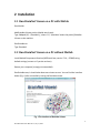
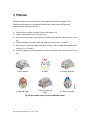
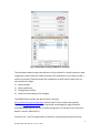
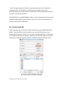
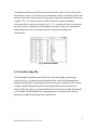
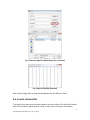
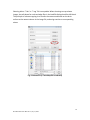
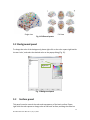
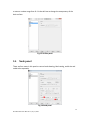
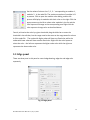
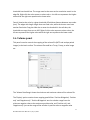
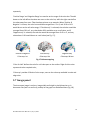
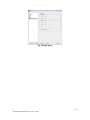
2011
BrainNet Viewer Manual
Mingrui Xia
National Key Laboratory of Cognitive
Neuroscience and Learning,
Beijing Normal University
7/11/2011
Contents
1
2
Introduction ................................................................................................................. 2
Installation.................................................................................................................... 3
2.1 Run BrainNet Viewer on a PC with Matlab ....................................................... 3
2.2 Run BrainNet Viewer on a PC without Matlab .................................................. 3
3 Pictures......................................................................................................................... 4
4 Load Files...................................................................................................................... 5
4.1 Load a surface file .............................................................................................. 5
4.2 Load a node file ................................................................................................. 7
4.3 Load an edge file................................................................................................ 8
4.4 Load a volume file ............................................................................................. 9
5 Visualize option.......................................................................................................... 11
5.1 Layout panel .................................................................................................... 11
5.2 Background panel ............................................................................................ 12
5.3 Surface panel ................................................................................................... 12
5.4 Node panel ...................................................................................................... 13
5.5 Edge panel ....................................................................................................... 15
5.6 Volume panel ................................................................................................... 17
5.7 Image panel ..................................................................................................... 18
6 Menu .......................................................................................................................... 20
6.1 Files.................................................................................................................. 20
6.2 Option .............................................................................................................. 21
6.3 Visualize ........................................................................................................... 21
6.4 Tools ................................................................................................................. 21
6.5 Help.................................................................................................................. 22
7 Toolbar ....................................................................................................................... 23
7.1 Load Files & Save as Image .............................................................................. 23
7.2 Print & Zoom ................................................................................................... 23
7.3 Move, Rotate & Get position ........................................................................... 24
7.4 Standard view .................................................................................................. 24
7.5 Demo ............................................................................................................... 25
Acknowledgements ........................................................................................................... 26
BrainNet Viewer User Manual 1.0, July 11, 2011
1
1 Introduction
BrainNet Viewer is a brain network visualization tool, which can help researchers to
visualize structural and functional connectivity patterns from different levels in a quick,
easy and flexible way. It would be greatly appreciated if you have any suggestions about
the package or manual.
Developed by Mingrui Xia,
National Key Laboratory of Cognitive Neuroscience and Learning,
Beijing Normal University, China
Contact information:
Mingrui Xia: [email protected]
Yong He: [email protected]; [email protected]
Please cite as ‘... was/were visualized with the BrainNet Viewer
(http://www.nitrc.org/projects/bnv/)’ while using the package to make publicized
pictures.
Copyright © 2011 Dr. Yong He’s Lab, National Key Laboratory of Cognitive Neuroscience
and Learning, Beijing Normal University, Beijing, China.
BrainNet Viewer User Manual 1.0, July 11, 2011
2
2 Installation
2.1 Run BrainNet Viewer on a PC with Matlab
Run Matlab.
Add BrainNet Viewer path to Matlab search path:
Type ‘Addpath(‘X:\...\BrainNet’);’, where ‘X:\...\BrainNet’ means the path of BrainNet
Viewer on the machine.
Run BrainNet.m:
Type ‘BrainNet’.
2.2 Run BrainNet Viewer on a PC without Matlab
Install Matlab Components Runtime (MCRInstall.exe, version 7.14, ~170MB) using
default settings (contact us if you do not have).
Restart your computer (strongly recommended).
Run BrainNet.exe, it should take about one minute to start. You can find the interface
below (Fig. 1) after successfully running the BrainNet viewer.
Fig. 1 The Interface of BrainNet Viewer
BrainNet Viewer User Manual 1.0, July 11, 2011
3
3 Pictures
BrainNet Viewer will not load surface, node, edge and volume file together. The
following combinations are acceptable and different combinations will generate
different network pictures (see Fig. 2):
1) Brain surface: load brain surface file only. See section 4.1;
2) Nodes: load node file only. See section 4.2;
3) Brain surface and nodes: load both brain surface and node files. See sections 4.1 and
4.2;
4) Nodes and edges: load both node and edge files. See sections 4.2 and 4.3;
5) Brain surface, nodes and edges: load brain surface, node and edge files together. See
sections 4.1, 4.2 and 4.3;
6) Volume mapping to surface: load brain surface and volume files. See section 4.1 and
4.4.
1) Brain Surface
2) Nodes
3) Surface & Nodes
5) Surface, Nodes &
6) Surface mapping
Edges
Fig. 2 Brain network pictures with the BrainNet viewer
4) Nodes & Edges
BrainNet Viewer User Manual 1.0, July 11, 2011
4
4 Load Files
To draw a brain network graph, some kinds of files such as brain surface, node file or
edge file should be loaded in the first step. Click ‘Load File’ button on the toolbar or
‘File\Load File’ in the menu to open Load File dialog shown below (Fig. 3). Select files to
draw required graph.
In BrainNet Viewer, we provided several brain surface templates and example files
(which were made from various brain parcellation methods). They include (1) ICBM152
whole-brain surface, Colin brain surface and ICBM152 left and right hemispheric surfaces
in the folder ‘.\Data\SurfTemplate’ and (2) node and edge files of AAL90, Brodmann82,
HOA112, Dos160 (160 ROIs from Dosenbach et al., Science 2010) and others (e.g.,
customized ROIs by users) in the folder ‘.\Data\ExampleFiles’.
Fig. 3 Load File dialog
4.1 Load a surface file
Click the ‘Browse…’ button next to the ‘Surface file’ in the ‘Load File’ dialog, and then
select the required brain surface file in the popup dialog. BrainNet Viewer provides two
different brain templates, ICBM152 (.\Data\SurfTemplate\BrainMesh_ICBM152.nv) and
Colin27 (.\Data\SurfTemplate\BrainMesh_ch2.nv), and separate hemisphere surfaces
(.\Data\SurfTemplate\ICBM152Left.nv, ICBM152Right.nv). In the below example, the
ICBM152 template is selected (Fig. 4).
BrainNet Viewer User Manual 1.0, July 11, 2011
5
Fig. 4 Select brain surface (ICBM152 is selected)
The information below is about the definition of the surface file. Usually, you don’t need
to generate a new surface file. Please read the file if interested or if you want to make a
surface by yourself. The brain surface file is defined as an ASCII text file with suffix ‘nv’
and contains four fields:
1) Vertex number;
2) Vertex coordinate;
3) Triangle faces number;
4) Index of vertex making up the triangles.
The ICBM152 brain surface was derived from Freesurfer
(http://surfer.nmr.mgh.harvard.edu/) and the Colin27 brain surface was made by
BrainVISA (http://brainvisa.info/). We transferred and merged the original bilateral
hemisphere files into one ‘.nv’ file. A surface merge tool is in the tools menu (see more
details in section ‘Menus\Tool’).
Currently, the ‘*.pial’ files generated by FreeSurfer, (only hemisphere mesh) and the
BrainNet Viewer User Manual 1.0, July 11, 2011
6
‘*.mesh’ files generated by BrainVISA are supported, and these can be loaded and
visualized directly. The FreeSurfer pial files are recommended as their vertex
coordinates have been transformed into the MNI space, while the BrainVISA mesh files
may need a manual transformation.
The ICBM152Left.nv and ICBM152Right.nv files are from Professor Alan Evans’s group in
the Montreal Neurological Institute, McGill University. Of note, the coordinates in the
surfaces are located in the MNI space.
4.2 Load a node file
The file represents the information from ROIs obtained from the AAL90, Brodmann82,
HOA112, Dos160 (160 ROIs from Dosenbach et al., Science 2010) and others (e.g.,
customized ROIs by users). Each file is in the folder ‘.\Data\ExampleFiles\’ corresponding
to its template name. Click the ‘Browse…’ button next to ‘Data file (node)’ in the Load
File dialog and select the required node file. The AAL90 node file is selected in Fig. 5.
Fig. 5 Select node file (AAL90 is selected)
BrainNet Viewer User Manual 1.0, July 11, 2011
7
The node file is defined as an ASCII text file with the suffix ‘node’. In the node file, there
are 6 columns: column 1-3 represent node coordinates, column 4 represents node colors,
column 5 represents node sizes, and the last column represents node labels. Please note,
a symbol ‘-‘(no ‘’) in column 6 means no labels. The user may put the modular
information of the nodes into column 4, like ‘1, 2, 3…’ or other information to be shown
by color. Column 5 could be set as nodal degree, centrality, T-value, etc. to emphasize
nodal differences by size. You can generate your nodal file according to the
requirements.
Fig. 6 Node file (AAL90)
4.3 Load an edge file
The brain edge file is defined as an ASCII text file with suffix ‘edge’, representing a
connectivity (e.g., correlations) matrix among the ROIs, which could be weighted or
binarized, and therefore, the dimensions of the matrix must correspond to the number
of nodes. AAL90, Brodmann82, HOA112, Dos160 (160 ROIs from Dosenbach et al.,
Science 2010) and other (e.g., customized ROIs by users) files are provided, and each file
is in the folder ‘.\Data\ExampleFiles\’ corresponding to its template name. You can
generate your edge file according to the requirements.
BrainNet Viewer User Manual 1.0, July 11, 2011
8
Fig. 7 Select an edge file (AAL90 binary file is selected)
Fig. 8 Edge file (AAL90, Binarized)
Both node and edge files can be generated/edited with text editors or Excel.
4.4 Load a volume file
This function lets users map the volume data to the brain surface. The volume file should
be a NIFTI paired file, which could be T-map, Z-map, atlas or any other volume data.
BrainNet Viewer User Manual 1.0, July 11, 2011
9
Selecting either ‘*.hdr’ or ‘*.img’ file is acceptable. When choosing to map volume
images, the edit boxes for node and edge files in the load file dialog should be left blank.
The principle of volume mapping is to transfer the vertex coordinates on the brain
surface to the nearest volume in the image file, and assign vertices to corresponding
values.
Fig. 9 Volume file (a T test-Map file is selected)
BrainNet Viewer User Manual 1.0, July 11, 2011
10
5 Visualize option
The option panel has three parts (Fig. 10). The list box on the left includes ‘Layout’,
‘Background’, ‘Surface’, ‘Node’, ‘Edge’, ’Volume’ and ‘Image,’ which represent different
aspects of the figure. The main panel on the right shows the detailed options of each
part; click the text in the list box to change the panel. There are six buttons on the
bottom of the panel: use the ‘Load’ and ‘Save’ options to acquire or save a .mat file;
‘Reset’ to return all parameters to their original state; ‘OK’ or ‘Apply’ to draw graph and
‘Cancel’ to exit the panel without changes.
Fig. 10 Option panel
5.1 Layout panel
This panel is used to set the output view of the brain model. The ‘Single view’ option
shows only one brain model, and can be set as Sagittal, Axial or Coronal view , while the
‘Full view’ option provides six or eight (depending on whether the brain surface can be
divided into left and right hemispheres) brain models. See Fig. 10 and Fig. 11.
BrainNet Viewer User Manual 1.0, July 11, 2011
11
Single view
Full view
Fig. 11 Different layouts
5.2 Background panel
To change the color of the background, please right-click on the color square right beside
the text ‘color’, and select the desired color on the popup dialog (Fig. 12).
Right Click
Fig. 12 Background panel
5.3
Surface panel
This panel is used to control the color and transparency of the brain surface. Please
right-click the color square to change color of the brain surface; and drag the slider bar
BrainNet Viewer User Manual 1.0, July 11, 2011
12
or enter a number range from 0~1 in the edit box to change the transparency of the
brain surface.
Fig. 13 Surface panel
5.4
Node panel
There are four zones in this panel to control node drawing, label setting, nodal size and
nodal color separately.
Fig. 14 Node panel
BrainNet Viewer User Manual 1.0, July 11, 2011
13
Draw nodes:
This function is used to decide which nodes are to be drawn. Select ‘Draw All’ to draw all
nodes in the file, or set a threshold of color or size corresponding to column 4 or column
5 to draw those nodes with higher value than the threshold.
Nodal label:
This panel is used to control the nodal label. Three options are available: ‘Label All’,
‘Label None’ or by a threshold that only label those nodes with higher value than the
threshold on size or color. Click the ‘Font…’ button to change the font of the labels in the
popup dialog.
Nodal size:
There are two ways to set the size of the nodes:
First, use the value in column 5 in the node file. In this manner, you can choose ‘Auto’ to
arrange the sizes of nodes to a proper range (radius: 2-7) by their value automatically, or
choose ‘Raw’ to use the original value in column 5 in the node file. When a threshold is
selected, the nodes below the threshold will be a small size (radius: 1), while those
above threshold will display by their Auto/Raw size. Drag the slider bar or enter the
threshold in the edit box. The range must be the same as that in column 5 in the node
file.
Second, set all nodes to an equal size ignoring the size value in the file, and the size can
be defined in the edit box.
The volume ratio option is used to adjust the size of all nodes together, and the scale
factor ranges from 0.1 to 10.
Nodal color:
This panel provides four ways to control nodal color:
First, to use the same color for all nodes ignoring the color index in the file, right-click
the color square and select the required color from the popup dialog.
Second, use a color map to display the value of the nodes from low end
to high end corresponding to column 4 in the node file. 13 kinds of color
maps can be selected (see the right picture for detail).
Third, modular color can be used to display different nodal colors for different modules.
BrainNet Viewer User Manual 1.0, July 11, 2011
14
Set the values of column 4 as ‘1, 2, 3…’ corresponding to modular 1,
modular 2… in the node file. The maximum number of modules is21
at present. Click to open the modular color dialog, and the left
picture will display six modules with their color on the right. Click the
popup menus on the left to select other modules in the list and the
color square will change to the corresponding one. Right-click the
color square to change color as described above.
Fourth, to binarize the color by a given threshold, drag the slider bar or enter the
threshold in the edit box, but the range must be the same as the range stated in column
4 of the node file. The nodes with higher value will have one fixed color, while the
nodes with lower value will have another fixed color. Right-click the color square to
select the color – the left one represents the higher value color while the right one
represents the lower value color.
5.5 Edge panel
There are three parts in this panel to control edge drawing, edge size and edge color
separately.
Fig. 15 Edge panel
BrainNet Viewer User Manual 1.0, July 11, 2011
15
Draw Edge
This panel is used to extract edge information from the correlation matrix contained in
the edge file, and to decide whether all or parts of them are to be drawn. Select ‘Draw
All’ to extract and draw all edges (all values not equal to zero) in the correlation matrix;
select ‘Threshold’ to extract the edge above a threshold. This threshold can be set as a
value in the matrix or in the sparsity of the matrix. Check ‘Absolute value’ to extract the
absolute value of the matrix. Note that BrainNet Viewer will treat the value zero (0) in
the matrix as a null edge, and only the right upper triangle of the matrix will be
considered. Always remember to change the threshold when a weighted matrix is loaded,
or it will draw the full connection among the nodes, which would require a lot of time.
Edge size
There are two ways to set the size of edges (here, size means the radius of the edge);
First, employ the correlation matrix value in the edge file. In this manner, you can choose
‘Auto’ to assign the edge sizes a proper range (radius: 0.3-1.5) by their value
automatically or choose ‘Raw’ to use the original value of the correlation matrix in the
edge file. When a threshold is selected, the edges with values lower than the threshold
will have a fixed, smaller size while the edges above threshold will be shown as
Auto/Raw size. Drag the slider bar or enter the threshold into the edit box, but the range
must be the same as the correlation matrix in the edge file.
Second, set all edges to an equal size, and the size can be defined in the edit box.
The scale option is used to adjust the size of all edges together. The scale factor ranges
from 0.1 to 10.
Edge color
This panel provides four ways to control edge color:
First, to adopt the same color for all edges, right-click the color square and select the
required color from the popup dialog.
Second, use a colormap to render the value of the edge from low to high corresponding
to the values of the correlation matrix in the edge file. 13 kinds of colormaps, same as
the nodal colormaps can be selected.
Third, in order to binarize the color by a given threshold, drag the slider bar or enter the
BrainNet Viewer User Manual 1.0, July 11, 2011
16
threshold into the edit box. The range must be the same as the correlation matrix in the
edge file. Right-click the color square to select colors – the left one represents the higher
value while the right one represents the lower value.
Fourth, binarize the color by a given threshold of Euclidean distance between two nodes
(mm). The edges with longer length have one fixed color, while the shorter ones have
another fixed color. Drag the slider bar or enter the threshold in the edit box; the
threshold can range from zero to 100. Right-click the color square to select colors, the
left one represents the higher value while the right one represents the lower value.
5.6 Volume panel
This panel is used to control the mapping of the volume file (NIFTI and analyze paired
images) to the brain surface. The volume file could be a T-map, Z-map, an atlas image
etc.
Fig. 16 Volume panel
The ‘Volume Data Range’ shows the minimum and maximum values of the volume file.
The ‘Display’ option contains three mapping possibilities: ‘Positive & Negative’, ‘Positive
only’ and ‘Negative only’. ‘Positive & Negative’ sets the colorbar range from the
minimum negative value to the maximum positive value, and ‘Positive only’ and
‘Negative only’ just set the range of the colorbar in positive value or negative value
BrainNet Viewer User Manual 1.0, July 11, 2011
17
separately.
‘Positive Range’ and ‘Negative Range’ are used to set the range of the color bar. The edit
boxes on the left define the value near zero on the color bar, while the right ones define
the value away from zero. Take the above picture as an example. When ‘Positive &
Negative’ is chosen, the color bar would be arranged from -3 to 3, and -0.01 to 0.01
would be set as the null value range; if ‘Positive only’ is selected, the color bar would be
arranged from 0.01 to 3, any value below 0.01 would be set as a null value; and if
‘Negative only’ is selected, the color bar would be arranged from -0.01 to -3, and any
value above -0.01 would be set as a null value (see Fig. 17);
Positive & Negative
Colormap: Jet
Positive only
Colormap: Hot
Fig. 17 Volume mapping
Negative only
Colormap: Winter
‘Color for Null’ defines the color for null value part on the surface. Right-click the color
square and select required color;
‘Colormap’ provides 13 kinds of color maps, same as the colormap available in node and
edge color.
5.7 Image panel
The size output Image is set here. Image width and height in pixel dimension or in
document size (both cm and inch), and dpi of the graph can be defined here (Fig. 18).
BrainNet Viewer User Manual 1.0, July 11, 2011
18
Fig. 18 Image panel
BrainNet Viewer User Manual 1.0, July 11, 2011
19
6 Menu
6.1 Files
Load files:
Click to open load files panel (for more details, see Section ‘Load Files’).
Save Image:
After visualization, click here to save the present figure as an
image. At present, TIFF, BMP, EPS, JPEG and PNG image formats
are supported. The parameters of the image such as pixel
dimension, document size and dpi can be adjusted in the ‘Option panel\Image’. After the
image is saved, a message box appears (see right picture).
Save Movie:
This function helps users to save a demonstration movie for network visualization. It
produces a 12 seconds long, 30 FPS, 735×534, avi file in which the brain network
rotates clockwise in a circle, one degree per frame. This operation will take about 10
minutes. Please drink a cup of coffee to wait before playing the movie. Note that this
function should only be used in the ‘Single view’ layout. Pictures below show different
frames at different times. For an example, see
http://www.nitrc.org/docman/view.php/504/1023/Demo%20Video%20of%20Brain%20N
etwork%20(14M)
3s
6s
Fig. 19 Frames of the network movie
9s
Exit:
Click to exit BrainNet Viewer.
BrainNet Viewer User Manual 1.0, July 11, 2011
20
6.2 Option
Option:
Click to open the option panel (see more details in section ‘Visualize Option’).
Load Option:
Load a previously saved visualize option file.
Save Option:
Save current visualize option as a *.mat file.
6.3 Visualize
Redraw:
Clear figure and redraw network using the data and option last loaded.
Clear Figure:
Remove brain network and display the default information of BrainNet Viewer.
6.4 Tools
Merge Mesh:
This tool is used to merge the left and right hemisphere surface files extracted from
FreeSurfer (*.pial) or BrainVISA (*.mesh) from two separate files into one BrainNet
Viewer surface template file (*.nv), or to convert a one hemisphere surface file to a
BrainNet Viewer surface template file (*.nv). When both ‘Left Mesh’ and ‘Right Mesh’
files are selected, the new mesh will combine two hemisphere files into one file. If only
one of the input files is selected, the new mesh file will convert only that hemisphere file
(Fig .20).
Fig. 20 Merge Meshes tool
BrainNet Viewer User Manual 1.0, July 11, 2011
21
6.5 Help
Manual:
Open this manual for help.
About:
Show version, author and contact information of BrainNet Viewer in a dialog.
BrainNet Viewer User Manual 1.0, July 11, 2011
22
7 Toolbar
The toolbar (Fig. 21) provides frequently-used and interaction commands to operate the
brain network graph, most of them are not included in the menu.
Fig. 21 Toolbar
7.1 Load Files & Save as Image
These two commands are included in menu, see details in section ‘Load Files’, and
section ‘Menu\File\Save Images’.
7.2 Print & Zoom
The Print command lets users print the current graph conveniently. A print panel like the
one below will pop up after the Print button is clicked.
The Zoom in and Zoom out buttons help users to focus on the local or observe the global
status of brain network.
BrainNet Viewer User Manual 1.0, July 11, 2011
23
Print panel
Zoom in & Zoom out
Fig. 22 Print panel and Zoom function
7.3 Move, Rotate & Get position
Click the ‘Move’ button and drag the brain anywhere in the window.
When the ‘Rotate’ button is pressed, hold left button of the mouse and move mouse to
rotate the brain. When rotate button is deselected, the light cam in the window will
re-render the brain model depending on the current orientation.
Click the ‘Get position’ button, and then click on the surface of the brain to show the
coordinate of the vertex. Right click anywhere in the figure window, and select ‘Delete
All Datatips’ to remove all coordinate labels.
7.4 Standard view
Three standard views, sagittal, axial and coronal view buttons are available to help users
observe networks from different standard views quickly. These buttons should only be
used for ‘Single view’ visualized brain networks. Click twice to see the opposite side of
the brain.
BrainNet Viewer User Manual 1.0, July 11, 2011
24
Sagittal View
Axial View
Fig. 23 Standard views
Coronal View
7.5 Demo
Press the black triangle button to make the brain rotate clockwise until the black square
button is pressed. This function only works for ‘Single View’ visualizations.
BrainNet Viewer User Manual 1.0, July 11, 2011
25
Acknowledgements
We thank the following colleagues for their kind helps during BrainNet Viewer
developing and manual revising: Dr. Gaolang Gong, Dr. Ni Shu, Mr. Jinhui Wang, Mr. Teng
Xie, Mr. Qixiang Lin, Ms. Zhengjia Dai, Ms. Miao Cao and Ms. Jiaying Zhang, National Key
Laboratory of Cognitive Neuroscience and Learning, Beijing Normal University, China;
Professor Alan Evans, McGill University, Canada; Mr. Patrick Clark, Pennsylvania State
University, USA.
We also thank the developers of the following softwares and toolboxes whose source
codes or file formats were referenced during our package developing:
Matlab: http://www.mathworks.com/products/matlab/
SurfStat: http://www.math.mcgill.ca/keith/surfstat/
FreeSurfer: http://surfer.nmr.mgh.harvard.edu/
BrainVISA: http://brainvisa.info/
BrainNet Viewer User Manual 1.0, July 11, 2011
26