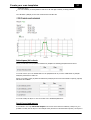
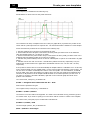
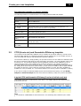
1
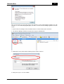
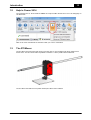
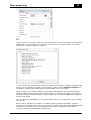
CT Dose Profiler
Probe for evaluation of CT systems
CT Dose Profiler User's Manual - English - Version 6.2A
RTI article number: 9630512-00
CT Dose Profiler User's Manual
2014-06-23/6.2A
CT Dose Profiler
The CT Dose Profiler probe makes it
possible to evaluate the performance of
modern CT scanners.
NOTICE
RTI Electronics AB reserves all rights to make changes in the CT Dose
Profiler, and the information in this document without prior notice.
RTI Electronics AB assumes no responsibility for any errors or
consequential damages that may result from the use or misinterpretation of
any information contained in this document.
Copyright © 2012-2014 by RTI Electronics AB. All rights reserved.
Content of this document may not be reproduced for any other purpose
than supporting the use of the product without prior permission from RTI
Electronics AB.
Microsoft, Microsoft Excel, Microsoft Access, Windows, Win32, Windows 95, 98, ME, NT, 2000, XP, 2003,
Vista, Windows 7 and Windows 8 are either registered trademarks or trademarks of Microsoft Corporation in
the United States and/or other countries.
OpenOffice.org and OpenOffice.org Calc are registred trademarks of OpenOffice.org.
BLUETOOTH is a trademark owned by Bluetooth SIG, Inc., USA.
Contact Information World-Wide
Contact Information United States
RTI Electronics AB
Flöjelbergsgatan 8 C
SE-431 37 MÖLNDAL
Sweden
RTI Electronics Inc.
33 Jacksonville Road, Building 1
Towaco, NJ 07082
USA
Phone: Int. +46 31 7463600
Phone: 800-222-7537 (Toll free)
Int. +1-973-439-0242
Fax: Int. +1-973-439-0248
E-mail
Sales: [email protected]
Support: [email protected]
Service: [email protected]
Web site: http://www.rti.se
E-mail
Sales: [email protected]
Support: [email protected]
Service: [email protected]
Web site: http://www.rtielectronics.com
CT Dose Profiler User's Manual
2014-06-23/6.2A
Intended Use of the CT Dose Profiler probe
Together with the Ocean Software from RTI Electronics AB it is to be used for quality control,
service and maintanance of CT systems.
With the CT system in stand-by condition without patients present, the probe is intended to be
used:
- to provide the operator with information on radiation beam parameters that might influence
further steps in an examination but not an ongoing exposure.
- for assessing the performance of the CT scanner.
- for evaluation of of examination techniques and procedures.
- for service and maintanance measurements.
- for quality control measurements.
- for educational purposes, authority supervision, etc.
The product is intended to be used by hospital physicists, X-ray engineers, manufacturer's
service teems, and other professionals with similar tasks and competencies. The operator need s
basic knowledge about the software Ocean before starting to use the CT Dose Profiler probe.
This can be achieved by studying the relevant documentation.
The product is NOT intended to be used:
- for direct control of any diagnostic X-ray system performance during irradiation of a patient.
- so that patients or other unquilified persons can change settings of operating parameters during
and immediately before and after measurements.
2014-06-23/6.2A
CT Dose Profiler User's Manual
CT Dose Profiler User's Manual
2014-06-23/6.2A
Contents
7
Table of Contents
1
2
3
4
5
6
Introduction
.............................................................................................................. 10
1.1
Users..............................................................................................................................
of the "old" software
10
1.2
Help in
Ocean 2014
..............................................................................................................................
13
1.3
The RTI
Mover
..............................................................................................................................
13
Start
..............................................................................................................
measuring
16
2.1
Make..............................................................................................................................
your first CTDI measurement
16
2.2
Measurement
free-in-air
..............................................................................................................................
24
2.3
Unlisted
CT scanners
..............................................................................................................................
26
Create
..............................................................................................................
your own templates
30
3.1
CTDI ..............................................................................................................................
template (in phantom)
30
3.2
CTDI ..............................................................................................................................
(free-in-air) and Geomtetric Efficiency template
35
Theory
.............................................................................................................. 42
4.1
CTDI ..............................................................................................................................
and k-factor
42
4.2
Why use
a k-factor?
..............................................................................................................................
44
The
..............................................................................................................
CT Dose Profiler Probe
46
5.1
Specifications
.............................................................................................................................. 46
5.2
Energy
correction
..............................................................................................................................
47
5.3
Angular
dependence
..............................................................................................................................
48
5.4
Rotation
symmetry
..............................................................................................................................
49
5.5
Field ..............................................................................................................................
size dependence
49
5.6
Axial sequential
scans vs. helical scans
..............................................................................................................................
50
Appendix
.............................................................................................................. 52
6.1
7
k-factors
.............................................................................................................................. 52
References
.............................................................................................................. 58
Index
................................................................................................................. 61
2014-06-23/6.2A
CT Dose Profiler User's Manual
CT Dose Profiler User's Manual
2014-06-23/6.2A
Chapter 1
Introduction
10
1
Introduction
Introduction
Regular quality assurance measurements on CT scanners are necessary in order to monitor the dose levels
patients are exposed to during medical examinations. In many countries, governments require regular
quality compliance testing information from clinics and hospitals that perform CT examinations.
Today, computed tomography (CT) comprises approximately 70% of the total dose given to patients
during X-ray examinations. With the rapid advancements in CT technology, there is increasing demand to
develop new testing strategies and measuring equipment to maintain the highest possible standard of
patient care. It was found that using the standard 10 cm CT ionization chamber may result in inaccurate
measurements due to its tendency to underestimate the dose profile. Our answer to this problem is the
CT Dose Profiler (CTDP) probe.
The CT Dose Profiler (CTDP) probe is a highly advanced point dose probe designed to fit into the
standard phantoms to evaluate computed tomography systems. There is no limit to the slice width that
users can measure with the CTDP. When using this probe for CTDI measurements, the traditional five
axial scans with an ion chamber are replaced with one helical (spiral) scan with the CTDP probe in the
center hole of the phantom (head or body). The CT Dose Profiler replaces the conventional TLD and OSL
methods or film for dose profile measurements.
The CT Dose Profiler probe is designed to be used with the Piranha X-ray multimeter and a PC running
the Ocean 2014 software. You can measure several different parameters with Ocean 2014 and the CTDP
probe. There are two standard templates, one for CTDI and one for geometric efficiency, that come
with Ocean 2014 which can be used with all license levels.
As mentioned above, the CTDI measurement can be done with one helical scan. After the helical scan,
Ocean 2014 gives several parameters at the same time such as CT dose profile, CTDI100, CTDIw ,
CTDIvol, DLP and FWHM.
The scientific methods used in the CT Dose Profiler have been evaluated in a variety of studies; see the
reference list (especially 1, 4, 10, 11, 12, 14, 15 and 16).
Note:
This manual will show you how to use the CT Dose Profiler probe with a Piranha and the Ocean 2014
software. It will also give examples of practical measuring methods. It is assumed that you have installed
Ocean 2014 and are familiar it. If you haven't installed Ocean 2014 yet, do that first. You will find
instructions in the Ocean 2014 User's Manual.
The CT Dose Profiler shall be handled with care even if it is much more durable than a traditional CT
ion chamber. If it is dropped or subjected to strong shocks, the detector chip may be damaged.
1.1
Users of the "old" software
Beginning October, 2012 Ocean software replaces the CT Dose Profile Analyzer software. All new CT
Dose Profiler probes from this date are delivered with the Ocean 2014 software. If you already have a
probe and are using the CT Dose Profile Analyzer software please note the following:
The first version of the CT dose profiler probe, called CT-SD16, will not work with Ocean 2014. If you
have this probe you have to continue to use the software you have or update to the new probe
called "CT Dose Profiler".
When you start Ocean 2014 for the first time with the CT Dose Profiler probe and you use Piranha,
Ocean 2014 may show a message that your probe needs to be reprogrammed:
CT Dose Profiler User's Manual
2014-06-23/6.2A
11
Introduction
Once you have done this, the probe will not work with the CT Dose Profiler Analyzer software (the "old"
software). To use it with this program again, you have to use the Detector Manager again and "reverse"
the fix:
1. Start the Detector Manager with the Piranha and the CD Dose Profiler probe connected.
2. The Detector Manager will show the probe and its type is "PiranhaCTDP":
3. Double-click on the probe and the following pop-up window is shown:
4. Change the type to "CT Dose Profiler".
2014-06-23/6.2A
CT Dose Profiler User's Manual
12
Introduction
5. Click on OK to close the window.
6. Now click on "Store to device":
7. Wait until programming of the probe is completed.
8. Close the Detector Manager. You can now use the probe with the CT Dose Profiler Analyzer ("old"
software) again.
Next time you use Ocean 2014 again and Ocean 2014 "complains" again and asks you to correct the
probe, you can follow the above procedure.
CT Dose Profiler User's Manual
2014-06-23/6.2A
13
Introduction
1.2
Help in Ocean 2014
The manual for the CT Dose Profiler is available as a help tutorial in Ocean 2014. Go to the Help page on
the ribbon bar:
Click on the CTDP tutorial button and select what you want to read about.
1.3
The RTI Mover
The RTI Mover is an accessory that can be used with the CT Dose Profiler Probe and is supported in
Ocean 2014. The RTI Mover makes it possible to measure CT dose profiles with an axial scan.
The RTI Mover is described in a separate manual, RTI Mover User's Manual.
2014-06-23/6.2A
CT Dose Profiler User's Manual
CT Dose Profiler User's Manual
2014-06-23/6.2A
Chapter 2
Start measuring
16
2
Start measuring
Start measuring
The Ocean 2014 software is used to evaluate and calculate all parameters based on the measured dose
profile. Ocean 2014 is available in three different license levels; Display, Connect and Professional.
Depending on the level you are running you have different possibilities.
Connect
You can use Quick Check or the templates that come with Ocean 2014. These templates are locked and
you cannot modify the structure. However, you can change set values and parameters that are used to
make the measurement and evaluate the result. You can only use real-time display mode.
Professional
You can use Quick Check or the templates that come with Ocean 2014 but you can also create your
own templates. This gives you more possibilities to adapt the templates to your own needs, add pass and
fail criteria and more. You can do both real-time display measurements and include the CT Dose Profiler
measurements in a QA session.
The CT Dose Profiler probe is a point dose detector that has a solid-state sensor placed 3 cm from the
end of the probe. The probe can be extended with an extension piece made of PMMA to fill different
phantoms. The extension is 45 mm. When this is attached, the detector will be centered in the middle
of a 150 mm wide PMMA phantom when the end of the extension reaches the end of the phantom.
The sensor is very thin (250 µm) in comparison to the beam width and is therefore always completely
irradiated when it is in the beam.
The sensor collects the dose profile. As radiation hits the sensor, in either direction, the detector
registers the dose value at that point and sends the information to the software. The electrometer can
collect 2000 such dose values per second. When the dose profile is collected all of the data points are
put into a graph. The recommended and most convenient method to measure the dose profile is to use
"Timed mode". This mode makes it possible to define exactly how long you want to measure and by that
being able to ensure that you don’t miss any radiation. You simply check on the CT scanner how long the
scan will take and then use a certain margin of your choice in specifying "measuring time".
To be able to collect the dose at the different positions, thereby creating the dose profile, the probe
must be moved through the CT beam. This is achieved by placing it free in air or in a phantom and then
using the couch movement to scan the probe (perform a helical scan). Therefore it is not possible to use
axial scans for measuring the CTDI with the CT Dose Profiler probe. You could, of course, make many
axial scans in small steps with the detector and plot a dose profile, but that takes a lot of time. With a
helical scan you will receive the dose profile in a few seconds. It has been proven that the CTDI can be
measured with helical scans as long as corrections are made for the pitch (see reference 10). This
correction is done automatically in Ocean 2014.
2.1
Make your first CTDI measurement
We will use the measuring template that comes with Ocean 2014 in this first example. As mentioned
before, it is assumed that you are familiar with Ocean 2014. If you need general information about Ocean
2014, please consult its User's Manual. You can do the measurement in Quick Check or in Ocean 2014's
main mode. If you use Quick Check, just follow the instructions on the screen but read in the text here
how to setup the phantom, probe and how to set the scanner.
Assume that you want to measure CTDI(100) using a head phantom:
First setup the meter, phantom and probe.
CT Dose Profiler User's Manual
2014-06-23/6.2A
17
Start measuring
1. Connect the CTDP probe to the Piranha via the extension cable. If you are using USB cable between
the meter and PC, connect it now.
2. Place the CT head phantom on the head support and the CTDP probe in the center hole with the
connector pointing towards the couch as shown in the picture.
Note: Only one exposure with the probe in the center hole is required. The section "Theory of
CTDI and k-factor" describes the theory behind this method.
3. Make sure that the sensor is in the center of the phantom. This can be accomplished easily by using
the graded scale on the CTDP probe. Assuming you are using a standard phantom with a length of 150
mm, the stitched mark at 75 mm on the CTDP probe should be place in the phantom opening and the
end of the extension should then be at the end of the phantom as shown in the pictures below:
4. Make sure that the two horizontal CT lasers are visible on the probe, approximately in the middle of it.
Also verify that the vertical laser is approximately in the middle of the phantom. Center the CT at this
position (put this position to zero).
5. Put a piece of tape along the probe, attaching it to the phantom. This is to ensure that the probe is
not dislodged within the phantom when the couch starts to move.
6. Start Ocean 2014.
7. Go to the Library tab and open the Examples(RTI) -> Application -> CT folder. (If you can't find
the examples, please read the section Import CT Dose Profiler templates.)
8. Select the template CTDI (CTDoseProfiler) by double-clicking on the name.
2014-06-23/6.2A
CT Dose Profiler User's Manual
18
Start measuring
9. A hint is shown that briefly describes how to perform the measurement. Click OK to close it (you can
reopen it by clicking on the hint icon). The template is loaded and a new measurement is initiated. Ocean
2014 will automatically connect to the meter at this point.
Note: Waveform grid, cursor data and analysis are empty right now, since no measurement has been
performed yet.
The template performs four different CTDI measurements (note only one exposure is needed for each
one), two with head phantom and two with body phantom. You can change Set kV and phantom type
if you want.
10. The first thing you should do is to select CT scanner in Ocean 2014. Go to the Equipment tab.
11. Specify the CT scanner manufacturer.
CT Dose Profiler User's Manual
2014-06-23/6.2A
Start measuring
19
12. Now select the CT scanner model. Click on the binoculars to see the CT scanner list for the specified
manufacturer. If you don't find your CT scanner in the list, select the "Generic scanner". You can also
read more in the section "Unlisted CT scanners".
13. Select CT scanner model and click OK. Note also that for each model the possible kV settings are also
listed. If you can't find the CT scanner you are looking for, read the section Unlisted CT scanners. For
the purpose of following this example select one that is similar to the one you have.
When you select the CT scanner model the required data will be pulled into your measurement from a
database including energy correction factors and the k-factor. You can read more about the k-factor in
the section "Theory of CTDI and k-factor". A more complete list of k-factors is available in the "Appendix"
section of this manual.
14. If you know the total filtration, go to the Tube tab and enter it. If you don't know, use the default
value (7 mm).
Now it is time to prepare the CT settings. You will be required to perform the following: perform a
topogram (a scout image), know how to set the cursors to define the scan area for the spiral/helical scan
and be able to perform the scan. It is very important that these CT-parameters are read and set
correctly; otherwise the measurement will be incorrect.
2014-06-23/6.2A
CT Dose Profiler User's Manual
20
Start measuring
15. First, perform a topogram (scout image) over the whole CT Dose Profiler when it is positioned inside
the phantom. Ocean 2014 is not used at this stage and the meter will not record any data. You do not
have to be concerned with any settings or measured data since the reason for this scan is to find out
where to set the cursors of the CT machine for the helical scan.
16. The CT console will show the scanned image similar to the one below.
Locate the sensor in the scanned image. Set the start cursor approximately 3 cm before the phantom
and the end cursor approximately 3 cm after the phantom. While these are not exact numbers the
measurement should start a little bit before the phantom and stop a little bit after it. Note down the
scan time that the CT unit needs to perform this scan as you will need this value later on to select a
suitable measuring time.
17. You must enter the following parameters before you can perform your first measurement.
-
kV
Pitch (-)
Tube rotation time (s)
Collimation (mm)
Phantom type (head or body)
To be able to acquire DLP you also need to specify:
- Scan length (mm)
The scan speed is automatically calculated.
You now have to find the corresponding parameters on the CT console. Parameters may have different
names on units from different manufacturers.
18. First select spiral/helical scan on the CT scanner.
19. Choose the correct Scan Field of View (SFOV) on the CT console. The SFOV should be chosen
according to the type of phantom that is used. Select the phantom type in Ocean 2014.
Here is an example of how a console may appear on a GE CT scanner when SFOV is selected.
CT Dose Profiler User's Manual
2014-06-23/6.2A
Start measuring
21
Select SFOV according to what kind of phantom you use:
Set values on the console:
2014-06-23/6.2A
CT Dose Profiler User's Manual
22
Start measuring
20. Select the kV at which you want to do the measurement and enter it into Ocean 2014. Select one
of the supported kVs that was shown when you selected the scanner model (see point #12).
21. Select the pitch and enter it into Ocean 2014.
22. Select the tube rotation time and enter it into Ocean 2014.
23. Select Collimation and enter it into Ocean 2014. Ocean 2014 defines Collimation as the total width of
the beam, the number of slices multiplied by the width of each slice.
24. Make sure to select "A(center)" for the "CT phantom position" in Ocean 2014.
25. If you want DLP, enter the scan length into Ocean 2014.
26. Make sure that the "Measuring time" is set to the same or a slightly larger value than the scan time
you noted in point #16 (if you specify a longer measuring time than you actually need, you lose
resolution in the dose profile).
You are now ready to perform the measurement. Timed mode will be used and you must start the
measurement manually before you start the CT scan.
27. Click the Start button in Ocean 2014 and begin the CT scan from the console.
28. You will see how the measurement is progressing on Ocean 2014's status bar.
The dose profile will now be measured. Be sure that the entire scan is covered by the measuring time
you have chosen. If not, you should increase the measuring time in Ocean 2014 and redo the
measurement.
29. As soon the measurement is completed Ocean 2014 will display the dose profile and calculated data.
The dose profile is shown in the waveform window and the total measured dose is shown in the
Exposure column in the grid.
CT Dose Profiler User's Manual
2014-06-23/6.2A
Start measuring
23
Make the necessary adjustments and redo the measurement if you don't get a value in the Exposure
column.
The waveform graph shows the dose profile:
There are two cursors that can be moved. Corresponding cursor values are shown in the waveform data
window.
The center indicator can be moved manually. This can be useful in situations when Ocean 2014 isn't able
to find the correct center position. When the center indicator is moved all values related to its position
and the +/-50 mm indications are recalculated. To move the center indicator just move mouse pointer
over it and use drag-and-drop. Right-click on the graph and select Auto-position center indicator if
you want to restore the automatically calculated position.
30. The calculated values are shown in the Analysis window.
2014-06-23/6.2A
CT Dose Profiler User's Manual
24
Start measuring
31. The first CTDI measurement is now done. You can now measure the remaining CTDI values using the
above method.
2.2
Measurement free-in-air
The second standard template that comes with Ocean 2014 is for measurements free-in-air. This
template calculates CTDI free-in-air and Geometric Efficiency. You perform this measurement the same
way as described in the previous section but in this case is no phantom used.
Hint
When you do the free-in-air measurement, you may use the phantom as a holder for the probe as shown
in the picture below:
1. Go to the Library tab and open the Examples(RTI) -> Application -> CT folder. (If you can't find
the examples, please read the section Load CT Dose Profiler templates.)
2. Select the template Geometric Efficiency (CTDoseProfiler) by double-clicking on the name.
CT Dose Profiler User's Manual
2014-06-23/6.2A
25
Start measuring
3. Load the template.
4. You must enter the parameters below before you can perform your first measurement.
-
kV
Pitch (-)
Tube rotation time (s)
Collimation (mm)
5. Now perform the measurement the same way as the CTDI measurement described in the previous
section.
6. As soon the measurement is completed Ocean 2014 will display the dose profile and calculated data.
The dose profile is shown in the waveform window and the total measured dose is shown in the
Exposure column in the grid.
Make the necessary adjustments and redo the measurement if you don't get a value in the Exposure
column.
The waveform graph shows the dose profile:
2014-06-23/6.2A
CT Dose Profiler User's Manual
26
Start measuring
There are two cursors that can be moved. Corresponding cursor values are shown in the waveform data
window.
If the center point and FWHM can't be found automatically the analysis will show a calculation error. In
this case, in the waveform graph (not the analysis graph), use the mouse pointer and grab the center
pointer. You can now move it. Position it manually in the center of the dose profile. Two new indicators,
for FWHM, become visible. Move these and position in a position where the dose rate is half of the
maximum dose rate.Now are all parameters in the analysis calculated based on the manual positions you
have done. If you want to go back to automatic calculation; right-click on the waveform graph and check
"Auto-position center indicator".
7. The calculated values are shown in the Analysis window.
8. The first measurement Geometric Efficiency is now done. Other parameters measured with this
template are the CTDI(100) free-in-air and the Beam width (FWHM = Full Width Half Maximum).
2.3
Unlisted CT scanners
The scanners we currently have k-factors for (required for the method to measure CTDI with only one
scan) are listed in Appendix k-factors. Note that you can always specify the k-factor after the
measurement if you don't know it when you perform the measurement. Add a user-defined k-factor later
and specify it. all calculations will be updated according to the new k-factor you specify.
As described in section Make your first CTDI measurement you select the CT scanner by clicking on the
binoculars on the Equipment tab after specifying the manufacturer name.
CT Dose Profiler User's Manual
2014-06-23/6.2A
27
Start measuring
When you click on the binoculars the available scanners for selected manufacturer are shown:
If you don't find the scanner model you are looking for do the following:
Select one that is similar to one in the list
Use the Generic scanner
Use your own k-factor. You must then instead select the CTDI template in the folder User-def kfactors or if you are using Ocean 2014 Professional, modify the template and add a column for the kfactor.
Select one that is similar
1. Select one that you think is similar.
2. Edit the model field.
3. Proceed according to the description in section Make your first CTDI measurement.
2014-06-23/6.2A
CT Dose Profiler User's Manual
28
Start measuring
Select "Generic scanner"
1. Select the "Generic scanner".
2. Edit the model field.
3. Proceed according to the description in section Make your first CTDI measurement.
Use your own k-factor
The k-factor is used by Ocean 2014 to calculate the weighted CTDI (CTDIw) from only one measurement
in the center hole of the phantom. The k-factor is calculated as:
If you know this factor for a certain CT scanner, you can use it by building your own template and include
the k-factor column:
As soon as you enter a value in the k-factor column, this value is used for the calculation. It will overrule
any value available in Ocean 2014's database.
CT Dose Profiler User's Manual
2014-06-23/6.2A
Chapter 3
Create your own templates
30
3
Create your own templates
Create your own templates
The templates we have used so far have been the standard templates delivered with Ocean 2014.
These templates are locked and cannot be modified (you can only change existing set values but not the
structure). You can build your own templates, real-time display or test templates, if you have Ocean
2014 Professional.
Ocean 2014's helptext and User's Manual give a general description of how to create a template. The
next two topics give specific information about required columns, calculations and other information
required to measure CTDI and Geometric Efficiency using the CT Dose Profiler and Ocean 2014.
3.1
CTDI template (in phantom)
The theory behind the method of only one helical scan with the probe in the center hole of the
phantom used in Ocean 2014 to measure the CTDI is described in the section CTDI and k-factor. This
section describes what columns and analyses you must include in a template to evaluate CTDI100, CTDIw ,
CTDIvol and DLP.
The CTDI analysis is used to evaluate the CT dose index on computed tomography systems using the RTI
CT Dose Profiler detector. Ocean 2014 uses one helical scan exposure with the CTDP in the center hole
of a 5-hole phantom and calculates the CTDIw , CTDIvol and DLP. Since a known relationship exists
between the the center hole and the peripheral holes, only one helical scan measurement is done in the
center hole of the phantom to calculate the CTDI. This relationship is unique for each CT scanner and is
defined in Ocean 2014 as the k-factor. A list of k-factors Ocean 2014 uses is available in the Appendix.
Use the binoculars to select a scanner from the list. Ocean 2014 will choose the correct k-factor based
the CT scanner name you selected.
If you want to modify the standard analysis (Ocean 2014 Professional is required), see topic Modify
analysis and Advanced analysis in the Ocean 2014 Reference Manual (or Help text).
A typical CTDI (in phantom helical scan)
This example shows three measurements, each with its own analysis. Two is a measurement in a head
phantom and the other is in a body phantom. In this case is only one measurement performed.
Note:
You should use TIMED MODE for this measurement. The measuring time is defined by the column
CT Dose Profiler User's Manual
2014-06-23/6.2A
31
Create your own templates
"Measuring time".
Use Low sensitivity for Head phantom and free-in-air and High sensitivity for Body phantom.
The calculation (analysis) for the first measurement looks like this:
Default pass/fail criteria
When you add the CTDI (in phantom helical scan) analysis the following pass/fail criteria is shown:
You must choose your own default limits for the pass/fail criteria. If you leave a limit blank no pass/fail
analysis is performed for that item.
When you modify a CTDI (in phantom helical scan) analysis (Ocean 2014 Professional is required), all pass/
fail criteria are available:
You must modify the layout to see the results of the additional parameters.
Result layout and macros
As described in the topic Advanced analysis in the Ocean 2014 Reference Manual (or Help text), it is
possible to modify the the layout of the analysis result (Ocean 2014 Professional is required). The layout is
2014-06-23/6.2A
CT Dose Profiler User's Manual
32
Create your own templates
defined as text combined with "macros". When the analysis result is shown, the macros are replaced
with the appropriate calculated values, set values and measured values. The default layout for the CTDI
(in phantom helical scan) analysis looks like this:
This text can be modified and more macros can be added to show more calculated results, for example,
the relative difference. The following macros are available for the CTDI (in phantom helical scan) analysis:
CT Dose Profiler User's Manual
2014-06-23/6.2A
Create your own templates
2014-06-23/6.2A
33
CT Dose Profiler User's Manual
34
Create your own templates
Calculations
The CTDI(100,c) is calculated in the following way:
All calculations are done from the dose profile waveform.
The waveform is an array of samples where the Z-axis (see graph above) represents the position of the
sensor and the y-axis represents the exposure rate. The waveform includes a maximum of 1024 samples.
Ocean 2014 finds key locations in the waveform in the following way:
1. Find the maximum dose rate that occurred during the scan.
2. Search backward from this point to find where the dose profile goes below 50% of the maximum
value and call this position X1 (not shown on graph).
3. Search forward from the point found in step 1 to find where the dose profile goes below 50% of the
maximum value and call this position X2 (not shown on graph).
4. Calculate the position halfway between X1 and X2. Call this point X3 (shown as a solid red line in graph
above).
5. Calculate "X3-50 mm" and "X3+50 mm" and call these positions X4 and X5, respectively. They are
marked with red dotted lines in the graph above and labeled with the text "-50 mm" and "+50 mm",
respectively.
If the points X1 and X2 can't be found automatically the analysis will show a calculation error. In this case,
in the waveform graph (not the analysis graph), use the mouse pointer and grab the center pointer. You
can now move it. Position it manually in the center of the dose profile. Two new indicators, for FWHM,
become visible. Move these and position in a position where the dose rate is half of the maximum dose
rate.Now are all parameters in the analysis calculated based on the manual positions you have done. If
you want to go back to automatic calculation; right-click on the waveform graph and check "Autoposition center indicator".
The central CTDI, CTDI(100,c) is calculated as:
$CTDIc = "Integrated dose between X4 and X5" * Pitch
Pitch must be specified in the grid.
The weighted CTDI, CTDI(100,w), is calculated as:
$CTDIw = $CTDIc * $kFactor
The k-factor is from the table in the Appendix. The k-factor is found based on kVp, phantom type and
CT scanner name. If you want to specify your own k-factor add the "k-factor" column to the template.
The volume CTDI, CTDI(100,vol) for a helical scan is calculated as:
$CTDIvol = $CTDIw / Pitch
The dose-length product, DLP, is calculated as:
$DLP = $CTDIvol * Scan length
CT Dose Profiler User's Manual
2014-06-23/6.2A
35
Create your own templates
Recommended columns (or general settings)
The following columns are recommended for the CTDI(in phantom helical scan) analysis.
Parameter
Description
Exposure(Measured)
The measured dose from the CT Dose Profiler detector.
Set kV
The set value for kV
CT Phantom type
(Set value)
The phantom type, specifies head or body for this analysis
CT phantom position
(Set value)
This specifies where the CT chamber is positioned in the phantom. ( n o t
re q u ire d , c e n t e r h o le is assu m e d if n o t sp e c ifie d)
Collimation (Set value) This column specifies the collimation.
3.2
Pitch (Set value)
This column specifies the pitch.
Scan length (Set
value)
This specifies the length of the scan.
Scan speed (Set
value)
This specifies the scan speed.
Measuring time
This is the measuring time for TIMED MODE. This is a meter setting (a value
used by the meter).
Tube rotation time
(Set value)
This is the tube rotation time.
CTDI (free-in-air) and Geomtetric Efficiency template
The CTDI (free-in-air helical scan) analysis is used to evaluate the geometric efficiency, CTDI free-in-air
and beam width (FWHM) on computed tomography systems using the RTI CT Dose Profiler detector. It
uses one helical scan exposure and calculates the geometric efficiency.
The Geometric efficiency is, simply speaking, the quotient between the dose inside the collimation width
NT and the total dose profile along the z-axis expressed in percentage. The exact definition can be seen
in reference 13. The Geometric efficiency gives an indication of how good the collimation on the CT
system is and how much of the radiation goes outside the detectors. An example of measured
Geometric efficiency is shown in the picture below. The two dotted black lines represent the length of
NT. Ideally, all the active detectors should receive the same amount of radiation and no radiation should
be outside the detectors. That would give a Geometric efficiency of 100%, but that is probably not
possible due to the penumbra, etc. A Geometric efficiency over 70% is good for a multi-slice CT (MSCT).
If you want to modify the standard analysis (Ocean 2014 Professional is required), see topic Modify
analysis and Advanced analysis in Ocean 2014 Reference Manual (or Help text) for more information.
A typical CTDI and Geometric Efficiency (free-in-air helical scan) test
This example shows three measurements, each with its own analysis. Only the first measurement is
performed in this case.
Note:
You should use TIMED MODE for this measurement. The measuring time is defined by the column
2014-06-23/6.2A
CT Dose Profiler User's Manual
36
Create your own templates
"Measuring time".
Use Low sensitivity for Head phantom and free-in-air and High sensitivity for Body phantom.
The calculation (analysis) for the first measurement looks like this:
Default pass/fail criteria
When you add the CTDI(helical scan/free-in-air) analysis the following pass/fail criteria is shown:
No default limits are specified, you must fill out limit. If you leave a limit blank not test for that criteria is
done.
Result layout and macros
As described in the topic Advanced analysis in the Ocean 2014 Reference Manual (or in the Help text),
it is possible to modify the the layout of the analysis result. The layout is defined as text combined with
"macros". When the analysis result is shown, the macros are replaced with the appropriate calculated
values, set values and measured values. The default layout of text CTDI (free-in-air helical scan) analysis
looks like this:
CT Dose Profiler User's Manual
2014-06-23/6.2A
Create your own templates
37
This text can be modified and more macros can be used to show more calculated results, for example the
relative difference. The following macros are available for the CTDI(free-in-air helical scan) analysis:
2014-06-23/6.2A
CT Dose Profiler User's Manual
38
Create your own templates
Calculations
The CTDI(100,c) is calculated in the following way:
All calculations are done from the dose profile waveform.
The waveform is an array of samples where the Z-axis (see graph above) represents the position of the
sensor and the y-axis represents the exposure rate. The waveform includes a maximum of 1024 samples.
Ocean 2014 finds key locations in the waveform in the following way:
1. Find the maximum dose rate that occurred during the scan.
2. Search backward from this point to find where the dose profile goes below 50% of the maximum
value and call this position X1 (not shown on graph).
3. Search forward from the point found in step 1 to find where the dose profile goes below 50% of the
maximum value and call this position X2 (not shown on graph).
4. Calculate the position halfway between X1 and X2. Call this point X3 (shown as a solid red line in graph
above).
5. Calculate "X3-50 mm" and "X3+50 mm" and call these positions X4 and X5, respectively. They are
marked with red dotted lines in the graph above and labeled with the text "-50 mm" and "+50 mm",
respectively.
If the points X1 and X2 can't be found automatically the analysis will show a calculation error. In this case,
in the waveform graph (not the analysis graph), use the mouse pointer and grab the center pointer. You
can now move it. Position it manually in the center of the dose profile. Two new indicators, for FWHM,
become visible. Move these and position in a position where the dose rate is half of the maximum dose
rate.Now are all parameters in the analysis calculated based on the manual positions you have done. If
you want to go back to automatic calculation; right-click on the waveform graph and check "Autoposition center indicator".
The central CTDI, CTDI(100,c) is calculated as:
$CTDI100 = "Integrated dose between X4 and X5" * Pitch
Pitch must be specified in the grid.
FWHM is calculated as the distance between X1 and X2:
$BeamWidthFWHM = X2 - X1
Calculate Geometric efficiency in the z-direction (according to IEC 60601-2-44) as:
$GeometricEfficiency = 100* (Dose between X6 and X7) / (Total dose)
Note!
The dose profile waveform is adjusted with the following function (X = FWHM) for 3 mm < X < 40 mm:
CorrF = 1.25466313 - 0.43935032 * X +0.34546921 * X2 - 0.14128364 * X3 + 0.03057638 * X4 0.00330919 * X5 + 0.00014071 * X6
For X < 3 mm, no valid correction available
CT Dose Profiler User's Manual
2014-06-23/6.2A
39
Create your own templates
For X > 40 mm, CorrF = 1.00
This means that the total dose indicated "between cursors" will differ from the dose value shown in the
grid (in the Exposure column) when the FWHM is less than 40 mm.
Recommended columns (or general settings)
The following columns are recommended for the CTDI (free-in-air helical scan) analysis.
Parameter
Description
Exposure(Measured)
The measured dose from the CT Dose Profiler detector.
Set kV
The set value for kV
CT Phantom type
(Set value)
The phantom type, specifies head or body for this analysis ( n o t re q u ire d)
Collimation (Set value) This column specifies the collimation.
Pitch (Set value)
This column specifies the pitch.
Scan length (Set
value)
This specifies the length of the scan. ( n o t re q u ire d)
Scan speed (Set
value)
This specifies the scan speed.
Measuring time
This is the measuring time for TIMED MODE. THis is a meter setting (a value
used by the meter).
Tube rotation time
(Set value)
This is the tube rotation time.
2014-06-23/6.2A
CT Dose Profiler User's Manual
CT Dose Profiler User's Manual
2014-06-23/6.2A
Chapter 4
Theory
42
Theory
4
Theory
4.1
CTDI and k-factor
A quick and convenient way to determine CTDIvol is to use a method we call the Central Point Method.
This method is based on the observation that the ratio between CTDIw and CTDI100,central is a constant
for specific CT scanners in combination with the type of phantom used in the measurement (see
reference 10). If the k-factor is known, you can perform a CTDI100(central) measurement and the
software will then calculate CTDIw and CTDIvol automatically. The Appendix k-factors lists all scanners
currently supported in Ocean 2014.
There are a number of different quantities related to CTDI. The most common are summarized in the
table below:
The CTDI quantity can be interpreted as the radiation energy deposited in a slice with a thickness
corresponding to the nominal beam collimation thickness. The dose inside the slice is the CTDI and the
dose outside the slice is excluded (see figure below).
In single slice CT the expression for CTDI is defined as:
where T is the nominal beam collimation thickness in mm and D(z) is the dose profile. On the y-axis the
quantity is relative dose. CTDI100 is acquired by reducing the integral to go between -50 and 50.
For MSCT, CTDI is defined as:
where N is the number of detectors and T is the width of a detector.
CTDIw (weighted) represents an average value of the CTDI100 inside a phantom (this requires five
measurements, one in each hole):
CT Dose Profiler User's Manual
2014-06-23/6.2A
43
Theory
In the case of single slice CT, the slice thickness is determined by the width of the detector. In multislice
CT (MSCT), the slice thickness is determined by the number of detectors and the widths of the
detectors.
In spiral CT there is an additional factor called the CT pitch factor. It is defined as the table movement
per gantry rotation:
where ∆d is the distance in mm that the couch moves between consecutive serial scans or per 360
rotation in helical scanning. N is the number of detectors and T is the detector thickness in mm (IEC
2003).
CTDIvol is the same as CTDIw but with respect to the pitch factor in helical (spiral) scanning:
The displayed CTDIvol given by a manufacturer may be a representative figure for that model and not the
value measured on the particular CT scanner (see reference 13).
The dose-length product, DLP, includes the irradiated volume and represents the overall exposure for an
examination and is calculated as following:
where L is the scan length of a certain examination.
The scan length is defined as:
where R is the number of tube rotations, p is the pitch factor, N is the number of detectors and T is the
detector thickness.
The effective dose to a region is defined as:
where DLP (mGycm) is defined in equation 6 and EDLP is the region specific, DLP normalized effective
dose (mSv/mGycm).
A quicker way to perform quality assurance has been introduced by using the CT Dose Profiler probe and
the Ocean 2014 software. To be able to use it, the k-factor must be known for the CT-unit and the
type of phantom that is used for the measurement. A number of k-factors for common CT-units are used
by the software and listed in the Appendix k-factors. The factor is calculated by dividing CTDIw with
CTDI100(central) from measurements obtained with pencil ion chambers:
For head phantoms the k-factor is around 1 and for body phantom the k-factor is around 1.7 at 120 kV.
2014-06-23/6.2A
CT Dose Profiler User's Manual
44
4.2
Theory
Why use a k-factor?
To measure the CTDI100 with the CT Dose Profiler in the center hole of a head or body phantom with
one helical scan exposure and then multiply it with the k-factor to get CTDIw and CTDIvol is, of course,
faster than doing the five exposures with the pencil ion chamber. With the CT Dose Profiler you can also
see a visible image of the dose profile that will tell you if something is wrong with the system. Another
reason why the k-factor should be used is that it is hard to compare axial measurements over a pencil ion
chamber with helical measurements over the CT Dose Profiler in the peripheral holes.
The nominal beam width is defined in the center of the CT where it is constant during the rotations. If
you move a detector outside the center axis the beam width and dose rate will oscillate during the
rotation. The pencil ion chamber is only partly irradiated so it is not affected the same way by the inverse
square law and divergence in the beam width as a fully irradiated detector. Measurements with the pencil
ion chamber do not tell you if you measure on a thin dose profile with high dose rate or a broad dose
profile with a low dose rate if they have the same dose area. It can only measure a value that can foretell
the dose but it cannot give a visible image of the dose profile.
The point dose detector can measure the same CTDI100 in the center of the CT with helical scans as
the pencil ion chamber can measure with axial scans. On the central axis the dose is non-oscillatory and
the beam width is constant. When measurements are performed in the peripheral holes the conditions
are not the same any more. The dose rate and the beam width in a peripheral hole oscillate during a
rotation. The dose rate oscillates due to varying x-ray attenuation and beam divergence with changing
distances affected by the inverse square law. The beam width varies due to the divergence from the xray source which becomes wider with increasing distance.
A single axial scan irradiates the same amount of dose to a detector with good rotation symmetry for
every full 360 degree rotation, it does not matter where the rotation starts and stops as long as it makes
one whole rotation and it is very easy to get good reproducibility. It is not the same for helical scans over
a point dose detector because then you measure the point dose and not the dose length of, for
example, 100 mm. The beam divergence from the x-ray source will have a big influence over the helical
dose distribution among the peripheral holes in the phantom. That makes it hard to measure reproducible
values if a suitable pitch is not used; a so called target pitch. The target pitch can be calculated with the
following equation:
where S is the distance between the x-ray source and CT center and R is the distance between the CT
center and the detector. Observe that you have to know the FWHM in the center of the CT. Few CTs
have the possibility to scan with any pitch value which makes it hard to perform this measurement. A
pencil ion chamber is not affected by the divergence in beam width and distance the same way as a
point detector. The CTDI100, p from a measurement with the pencil ion chamber and the point dose
detector are a little hard to compare but the point doses simulate the dose to a point in a phantom
better.
This is the reason why it is recommended to use the one exposure method with the k-factor.
CT Dose Profiler User's Manual
2014-06-23/6.2A
Chapter 5
The CT Dose Profiler Probe
46
5
The CT Dose Profiler Probe
The CT Dose Profiler Probe
The CT Dose Profiler has one solid-state sensor placed 3 cm from the end of the probe. The probe can
be extended with an extension piece made of PMMA to fill different phantoms. The standard extension is
45 mm. When this extension is on, the detector will be centered in the middle of a 150 mm wide PMMA
phantom when the end of the extension reaches the end of the phantom.
The sensor in the CT Dose Profiler probe is very thin (250 µm) in comparison to the beam width and is
therefore always completely irradiated when it is in the beam.
The sensor is used to collect the dose profile and it can also be used as a trigger. As radiation hits
SENSOR, in either direction, the detector registers the dose value at that point and sends the
information to the software. The electrometer can collect 2000 such dose values per second. The
recommended and most convenient method to measure the dose profile is to use the update mode
called Timed. This mode makes it possible to measure exactly the length of time you like. You simply
check on the CT-system how the scan will take and then use a margin in your choice of Measuring time.
To be able to collect the dose at the different positions, thereby creating the dose profile, the probe
must be moved through the CT. This is achieved by placing it free in air or in a phantom and then using
the couch movement to scan the probe. In short, do a helical (spiral) scan. Therefore it is not possible to
use axial scans for measuring CTDI with the CT Dose Profiler probe and Ocean 2014, since then the dose
profile is not measured. When the table is not moving, the CT Dose Profiler acts as an ordinary dose
detector and simply gives the point dose reading at that position. You can, of course, make many axial
scans in small steps with the detector and plot a dose profile, but that takes a lot of time. With a helical
scan you will receive the dose profile in a few seconds. It has been proven that the dose profile can be
measured with helical scans as long as corrections are made for the pitch (see reference 10).
5.1
Specifications
Supported meters:
Barracuda with EMM-1Ch, EMM-2Ch, EMM-Bias, EMMBiasB and EMM-BiasW (with Ocean)
Piranha with external input (with Ocean 2014)
Typical cal. factor:
0.28 mGy/nC
Material:
Al and PMMA
Connector:
Triaxial LEMO
Length (Detector + extension):
165 mm + 45 mm
Diameter:
12.5 mm
Sensor width:
250 um
Max sensitivity variation:
Less than ±5 %
Weight (Probe + extension):
40 g + 10 g
CT Dose Profiler User's Manual
2014-06-23/6.2A
47
The CT Dose Profiler Probe
5.2
Energy correction
When using the Piranha with Ocean 2014 and the CT Dose Profiler probe in the radiographic range, all
dose and rate values measured are automatically compensated for the energy dependence of the
sensor.
The kV range is 55-150 kV and the total filtration ranges from 1 to 55 mm Al for measurements free-inair and from 3 to 22 mm Al for measurements in head and body CT phantoms. The reference point for all
correction factors is at 120 kV with 2.5 mm Al filtration free-in-air (calibration R3 (RQR)).
Energy correction factors free-in-air (beam quality RQR)
Energy correction factors for Head Phantom (beam quality RQR)
2014-06-23/6.2A
CT Dose Profiler User's Manual
48
The CT Dose Profiler Probe
Energy correction factors for Body Phantom (beam quality RQR)
5.3
Angular dependence
This is a graph of the typical angular dependence of the CT Dose Profiler probe measured at 120 kV.
CT Dose Profiler User's Manual
2014-06-23/6.2A
49
The CT Dose Profiler Probe
5.4
Rotation symmetry
The rotation symmetry can be measured by rotating the CT Dose Profiler along its longest axis under an
irradiating x-ray tube. A typical rotation symmetry for one whole rotation is shown in picture below.
(the output from the tube was going down slightly during the long exposure)
Typical deviation for the CT Dose Profiler probe is about ± 1 %.
5.5
Field size dependence
The CT Dose Profiler probe is calibrated with a 5 cm wide field. When measurements are performed free
in air with small fields (< 4 cm and down to 3 mm) the calibration factor is no longer accurate and must
be corrected, see picture below. This is automatically done in Ocean 2014 when you measure free-in-air
and the FWHM lower then 4 cm.
No correction is needed in a phantom due to the large amount of scattering material.
2014-06-23/6.2A
CT Dose Profiler User's Manual
50
5.6
The CT Dose Profiler Probe
Axial sequential scans vs. helical scans
The two methods to receive a dose profile, axial sequential scans and helical scans, have been compared
and two dose profiles from the two methods are shown in the picture below. The measurement with
the axial sequential scans took a long time to perform and the helical scan took a couple of seconds. The
measurements were made in a phantom (without the couch in the beam).
CT Dose Profiler User's Manual
2014-06-23/6.2A
Chapter 6
Appendix
52
Appendix
6
Appendix
6.1
k-factors
The table below shows the k-factors Ocean uses. There bis one factor for head and body, respectively.
The k-factors are based on data from impactctscan.org.
Manufacturer
Elscint
Elscint
Elscint
Elscint
Elscint
GE
GE
GE
GE
GE
GE
GE
GE
GE
GE
GE
GE
GE
GE
GE
GE
GE
GE
GE
GE
GE
GE
GE
GE
GE
GE
GE
GE
GE
GE
GE
GE
GE
GE
GE
GE
GE
GE
GE
GE
GE
GE
GE
GE
GE
GE
GE
Name
Exel 2400 Elect
Exel 2400 Elect
CT Twin
Helicat
Generic scanner
8800/9000 Series
9800 Series
9800 Series
HiLight
HiLight
HiLight
HiLight
HiSpeed CT/i no SmartBeam
HiSpeed CT/i no SmartBeam
HiSpeed CT/i no SmartBeam
HiSpeed CT/i no SmartBeam
HiSpeed CT/i with SmartBeam
HiSpeed CT/i with SmartBeam
HiSpeed CT/i with SmartBeam
HiSpeed CT/i with SmartBeam
CT Max
Pace
Pace
Pace
Pace
Sytec
Sytec
Sytec
Sytec
Prospeed
Prospeed
FX/i
FX/i
FX/i
LX/i
LX/i
LX/i
QX/i
QX/i
QX/i
QX/i
LightSpeed
LightSpeed
LightSpeed
LightSpeed
LightSpeed Plus
LightSpeed Plus
LightSpeed Plus
LightSpeed Plus
HiSpeed ZX/i
HiSpeed ZX/i
HiSpeed ZX/i
CT Dose Profiler User's Manual
kVp
120
140
120
120
120
120
120
140
80
100
120
140
80
100
120
140
80
100
120
140
120
80
120
135
140
80
120
135
140
120
140
80
120
140
80
120
140
80
100
120
140
80
100
120
140
80
100
120
140
80
120
140
Head
1,069
1,047
1,047
1,050
0,962
1,038
1,020
1,047
1,008
1,030
1,015
1,047
1,008
1,030
1,015
1,047
1,008
1,030
1,015
0,961
1,162
1,053
1,041
1,061
1,162
1,053
1,041
1,061
1,052
1,040
1,145
1,058
1,037
1,145
1,058
1,037
1,032
0,999
0,987
0,977
1,032
0,999
0,987
0,977
1,032
0,999
0,987
0,977
1,027
0,993
0,968
Body
1,527
1,430
1,466
1,466
1,500
1,680
1,585
1,503
1,600
1,636
1,605
1,571
1,600
1,636
1,605
1,571
2,093
1,827
1,607
1,568
1,505
2,164
1,734
1,627
1,636
2,164
1,734
1,627
1,636
1,713
1,610
2,213
1,692
1,605
2,213
1,692
1,605
1,927
1,730
1,633
1,570
1,927
1,730
1,633
1,570
1,927
1,730
1,633
1,570
1,810
1,500
1,480
2014-06-23/6.2A
53
Appendix
GE
GE
GE
GE
GE
GE
GE
GE
GE
GE
GE
GE
GE
GE
GE
GE
GE
GE
GE
GE
GE
GE
GE
GE
GE
GE
GE
GE
GE
GE
GE
GE
GE
GE
GE
GE
GE
Philips
Philips
Philips
Philips
Philips
Philips
Philips
Philips
Philips
Philips
Philips
Philips
Philips
Philips
Philips
Philips
Philips
Philips
Philips
Philips
Philips
Philips
Philips
Philips
Philips
2014-06-23/6.2A
HiSpeed NX/i
HiSpeed NX/i
HiSpeed NX/i
LightSpeed Ultra
LightSpeed Ultra
LightSpeed Ultra
LightSpeed Ultra
LightSpeed 16
LightSpeed 16
LightSpeed 16
LightSpeed 16
LightSpeed Pro 16
LightSpeed Pro 16
LightSpeed Pro 16
LightSpeed Pro 16
LightSpeed RT
LightSpeed RT
LightSpeed RT
LightSpeed RT
LightSpeed VCT
LightSpeed VCT
LightSpeed VCT
LightSpeed VCT
LightSpeed VCT (small hd, large bd)
LightSpeed VCT (small hd, large bd)
LightSpeed VCT (small hd, large bd)
LightSpeed VCT (small hd, large bd)
Optima CT660
Optima CT660
Optima CT660
Optima CT660
Discovery CT750
Discovery CT750
Discovery CT750
Discovery CT750
Discovery CT750 (small, bd)
Generic scanner
Philips 310 (GE2, no Cu)
Philips 350 (GE2, no Cu)
Philips 310 (GE2, w. Cu)
Philips 350 (GE2, w. Cu)
Philips 310 (GE3, no Cu)
Philips 350 (GE3, no Cu)
Philips 310 (GE3, w. Cu)
Philips 350 (GE3, w. Cu)
Philips AV
Philips AV
Philips AV
Philips AV
Philips AV
Philips LX
Philips LX
Philips LX
Philips LX
Philips LX
Philips SR7000
Philips SR7000
Philips SR7000
Philips SR7000
Philips SR7000
Philips CX
Philips CX/S
80
120
140
80
100
120
140
80
100
120
140
80
100
120
140
80
100
120
140
80
100
120
140
80
100
120
140
80
100
120
140
80
100
120
140
120
120
120
120
120
120
120
120
120
120
80
100
120
130
140
80
100
120
130
140
80
100
120
130
140
120
120
1,027
0,993
0,968
1,042
1,009
0,994
0,985
1,046
1,010
0,993
0,984
1,057
1,013
0,994
0,983
1,093
1,052
1,028
1,015
1,136
1,088
1,066
1,048
1,061
1,022
1,004
0,993
0,949
0,965
1,111
1,090
1,084
1,050
1,089
1,089
1,025
1,025
1,810
1,500
1,480
2,009
1,787
1,656
1,614
1,819
1,627
1,611
1,483
1,996
1,771
1,652
1,577
2,140
1,897
1,770
1,694
2,046
1,778
1,648
1,566
2,041
1,802
1,684
1,614
2,010
1,810
1,700
1,650
2,100
1,850
1,730
1,670
1,560
1,700
1,956
1,956
1,120
1,061
1,061
1,066
1,048
1,120
1,061
1,061
1,066
1,048
1,120
1,061
1,061
1,066
1,048
1,059
1,059
2,034
1,795
1,718
1,739
1,666
2,034
1,795
1,718
1,739
1,666
2,034
1,795
1,718
1,739
1,666
1,572
1,572
CT Dose Profiler User's Manual
54
Appendix
Philips
Philips
Philips
Philips
Philips
Philips
Philips
Philips
Philips
Philips
Philips
Philips
Philips
Philips
Philips
Philips
Philips
Philips
Philips
Philips
Philips
Philips
Philips
Picker
Picker
Picker
Picker
Picker
Picker
Picker
Picker
Picker
Picker
Picker
Picker
Picker
Philips
Marconi
Marconi
Marconi
Marconi
Marconi
Marconi
Shimadzu
Shimadzu
Shimadzu
Shimadzu
Siemens
Siemens
Siemens
Siemens
Siemens
Siemens
Siemens
Siemens
Siemens
Siemens
Siemens
Siemens
Siemens
Siemens
Siemens
Philips SR4000
Philips SR 5000
Philips SR 5000
Philips M/EG
Philips M/EG
Philips TX
Philips TX
Philips TX
Philips CT Secura
Philips CT Secura
Philips Mx8000
Philips Mx8000
Philips Mx8000
Philips AcQSim
Philips AcQSim
Mx8000 IDT/Brilliance 16 (& Power)
Mx8000 IDT/Brilliance 16 (& Power)
Mx8000 IDT/Brilliance 16 (& Power)
Philips Aura
Philips Big Bore
Philips Big Bore
Philips Big Bore
Generic scanner
Picker 1200SX
Picker 1200SX
Picker 1200SX
Picker 1200SX
Picker PQ Series
Picker PQ Series
Picker PQ Series
Picker UltraZ
Picker UltraZ
Picker UltraZ
Picker UltraZ
Picker UltraZ
Generic scanner
Philips/Marconi Mx8000
Marconi Mx8000
Marconi Mx8000
Marconi Mx8000
Marconi AcQSim
Marconi AcQSim
Generic scanner
Shimadzu SCT
Shimadzu SCT
Shimadzu SCT
Generic scanner
Siemens CR
Siemens CR512
Siemens DRH
Siemens Somatom 2
Siemens DR1/2/3
Siemens DRG
Siemens DRG1
Somatom Plus 4 Series
Somatom Plus 4 Series
Somatom Plus 4 Series
Somatom AR-C
Somatom AR-C
Somatom AR.SP
Somatom AR.SP
Somatom AR-T
CT Dose Profiler User's Manual
120
120
130
120
130
100
120
130
120
140
90
120
140
120
130
90
120
140
120
90
120
140
120
80
120
130
140
120
130
140
80
100
120
130
140
120
90
90
120
140
120
130
120
80
120
130
120
125
125
125
125
125
125
125
80
120
140
110
130
110
130
110
1,053
1,065
1,052
1,199
1,196
1,724
1,768
1,886
2,640
2,631
1,038
1,060
1,052
1,096
1,061
1,130
1,114
1,100
1,134
1,079
1,070
1,070
1,121
1,121
1,121
1,117
1,117
1,688
1,638
1,888
1,683
1,653
2,057
1,983
1,765
1,623
1,554
1,667
1,996
1,778
1,718
1,700
3,008
2,087
2,053
1,938
1,960
2,053
1,937
3,328
2,185
1,955
1,926
1,868
1,900
1,888
1,888
1,683
1,653
2,057
1,983
1,750
2,470
1,992
1,984
1,900
2,164
2,164
2,164
2,190
2,190
1,100
1,075
1,062
1,076
1,067
1,076
1,067
1,076
2,047
1,782
1,738
1,817
1,736
1,817
1,736
1,817
1,130
1,114
1,072
1,059
1,062
1,114
1,113
1,083
1,063
1,060
0,950
1,018
0,895
0,966
0,950
0,950
1,076
1,047
0,977
0,965
0,960
1,000
1,096
1,096
1,061
2014-06-23/6.2A
55
Appendix
Siemens
Siemens
Siemens
Siemens
Siemens
Siemens
Siemens
Siemens
Siemens
Siemens
Siemens
Siemens
Siemens
Siemens
Siemens
Siemens
Siemens
Siemens
Siemens
Siemens
Siemens
Siemens
Siemens
Siemens
Siemens
Siemens
Siemens
Siemens
Siemens
Siemens
Siemens
Siemens
Siemens
Siemens
Siemens
Siemens
Siemens
Siemens
Siemens
Siemens
Siemens
Siemens
Siemens
Siemens
Siemens
Siemens
Siemens
Siemens
Siemens
Siemens
Siemens
Siemens
Siemens
Toshiba
Toshiba
Toshiba
Toshiba
Toshiba
Toshiba
Toshiba
Toshiba
Toshiba
2014-06-23/6.2A
Somatom AR-T
Siemens AR.HP
Siemens Plus
Siemens Plus
Siemens DXP
Siemens DXP
Siemens Plus-S
Siemens Plus-S
Siemens Hi Q
Siemens Balance
Siemens Balance
Siemens Emotion
Siemens Emotion
Siemens Volume Zoom
Siemens Volume Zoom
Siemens Volume Zoom
Access
Access
Access
Emotion Duo
Emotion Duo
Emotion Duo
Sensation 4
Sensation 4
Sensation 4
Sensation 16
Sensation 16
Sensation 16
Sensation 16
Sensation 16 Straton
Sensation 16 Straton
Sensation 16 Straton
Sensation 16 Straton
Emotion 6
Emotion 6
Emotion 6
Sensation 10
Sensation 10
Sensation 10
Sensation 10
Sensation Open
Sensation Open
Sensation Open
Sensation Open
Sensation 64
Sensation 64
Sensation 64
Sensation 64
Definition AS
Definition AS
Definition AS
Definition AS
Generic scanner
Toshiba TCT 600
Xspeed II
Xpress GX (Pre '98)
Xvision/EX
Xpress HS1
Xpress HS
Xpress GX (Post '98), Asteion
Xpress GX (Post '98), Asteion
Asteion
130
130
120
137
120
137
120
137
133
110
130
110
130
80
120
140
80
120
140
80
110
130
80
120
140
80
100
120
140
80
100
120
140
80
110
130
80
100
120
140
80
100
120
140
80
100
120
140
80
100
120
140
120
120
120
120
120
120
120
120
130
120
1,067
1,036
1,102
1,068
1,102
1,068
1,102
1,068
1,079
1,085
1,074
1,085
1,074
1,201
1,124
1,107
1,201
1,124
1,107
1,108
1,055
1,039
1,156
1,086
1,142
1,103
1,079
1,258
1,209
1,088
0,821
0,854
1,024
1,155
1,111
1,086
1,071
1,046
1,037
1,042
1,027
1,022
1,054
1,036
1,031
1,027
1,070
0,987
0,995
1,035
0,952
1,039
1,000
1,035
1,017
1,035
1,736
1,565
1,789
1,749
1,789
1,749
1,789
1,749
2,027
1,806
1,729
1,806
1,729
2,135
1,750
1,696
2,135
1,750
1,696
1,951
1,666
1,606
1,939
1,656
1,602
1,893
1,743
1,639
1,584
1,893
1,663
1,629
1,571
1,751
1,584
1,526
1,893
1,743
1,639
1,584
1,812
1,674
1,601
1,558
1,684
1,581
1,532
1,538
1,851
1,680
1,587
1,525
1,600
1,527
1,598
1,354
1,369
1,359
1,501
1,472
1,501
CT Dose Profiler User's Manual
56
Appendix
Toshiba
Toshiba
Toshiba
Toshiba
Toshiba
Toshiba
Toshiba
Toshiba
Toshiba
Toshiba
Toshiba
Toshiba
Toshiba
Toshiba
Toshiba
Toshiba
Toshiba
Toshiba
Toshiba
Toshiba
Toshiba
Asteion
Aquilion Multi/4
Aquilion Multi/4
Aquilion Multi/4
Aquilion Multi/4
Auklet
Asteion Multi (older tube)
Asteion Multi (older tube)
Asteion Multi (older tube)
Asteion Multi (older tube)
Asteion Multi (CXB-400C tube)
Asteion Multi (CXB-400C tube)
Asteion Multi (CXB-400C tube)
Asteion Multi (CXB-400C tube)
Asteion Dual
Asteion Dual
Aquilion 16
Aquilion 16
Aquilion 16
Aquilion 16
Generaic scanner
CT Dose Profiler User's Manual
130
80
100
120
135
120
80
100
120
135
80
100
120
135
120
135
80
100
120
135
120
1,017
1,117
1,079
1,057
1,034
1,019
1,141
1,099
1,076
1,062
1,141
1,099
1,076
1,062
1,117
1,070
1,147
1,070
1,056
1,051
1,050
1,472
2,072
1,846
1,728
1,672
1,470
2,131
2,039
1,731
1,841
2,131
2,039
1,731
1,841
1,857
1,685
2,206
1,959
1,779
1,728
1,700
2014-06-23/6.2A
Chapter 7
References
58
7
References
References
1. Vrieze, T., Bruesewitz, M.R., Primak, A., Zhang, J., McCollough, C. H. CT dosimetry:
A comparison of measurement techniques and devices. Department of Radiology,
Mayo Clinic College of Medicine. The study will be presented at RSNA 2006
2. Appendix MSCT Dosimetry, guidelines on radiation dose to the patient.
3. Karlsson, H. A new detector for measurements of CT dose profile, CTDI and CT
tube variations, Poster. Can be downloaded from http://www.rti.se in the section
“Application Notes”
4. Karlsson, H. Development and evaluation of a new detector and software for
measurements of CT dose profile, CTDI and CT tube current variations. Master
Thesis, Department of Radiation Physics, Göteborg University, Göteborg, Sweden 2004.
5. Nagel, H. D. Radiation Exposure in Computed Tomography. Fundamentals,
Influencing parameters, Dose Assessment, Optimisation, Scanner Data,
Terminology. 4th Edition, Hamburg, Germany, December 2002, CTB Publications, D21073 Hamburg, [email protected]
6. Stamm, G., Nagel, H. D. Software CT-Expo, Medizinische Hockschule Hannover, D30625 Hannover, [email protected]
7. International Standard IEC 61267, Medical diagnostic X-ray equipment – Radiation
conditions for use in the determination of characteristics. 1994
8. Morin, Gerber and McCollough, Radiation Dose in Computed Tomography of the
Heart by, American Hart Association, Inc 2003.
9. ACR Practice Guideline for Diagnostic Reference Levels in Medical X-Ray Imaging
2002 (Res. 20)
10. Cederquist, B. Evaluation of two thin CT dose profile detectors and a new way to
perform QA in a CTDI head phantom. Master Thesis, Department of Radiation
Physics, Göteborg University, Göteborg, Sweden 2008.
11. Vrieze, T., Bauhs, J., McCollogh, C. Use of spiral scan acquisition for CT dose
measurements: Selection of optical pitch values to ensure reproducible results, LLPH6115-B05, RSNA 2007 (abstract)
12. Herrnsdorf, L., Björk, M., Cederquist, B. and Mattsson, C., Thungström, G., Fröjdh, C.,
Point dose profile measurements using solid-state detectors in characterization of
Computed Tomography systems, RTI Electronics AB, Mölndal, Sweden and Mid
Sweden University, Sundsvall, Sweden
Science Direct; doi:10.1016/j.nima.2009.03.159
13. International Standard IEC 60601-2-44. Particular requirements for the safety of xray equipment for computed tomography, International Standard, Geneva,
Switzerland, International Electrotechnical Commission, 2002
CT Dose Profiler User's Manual
2014-06-23/6.2A
59
References
14. Perisinakis, K., Papadakis, A. E., Damilakis, J., The effect of x-ray beam quality and
geometry on radiation utilization efficiency in multidetector CT imaging, Medical
Physics, Vol. 36, No. 4, April 2009
15. Palm, Å., Herrnsdorf, L., Absorbed dose and dose rate using the Varian OBI 1.3 and
1.4 CBCT system. Journal of Applied Clinical Medical Physics
16. Dixon, R. L., A new look at CT dose measurement: Beyond CTDI, Med. Phys. 30 .6.,
June 2003. 0094-2405/2003/30.6./1272/9
17. Dixon, R. L., Restructuring CT dosimetry-A realistic strategy for the future Requiem
for the pencil chamber, Med. Phys. 33.10 October 2006. 00942405/2006/33(10)/3973/4/$23.00
Please find more information about the basis of the dose profile detector in these thesis works:
”Development and evaluation of a new detector and software for measuring CT dose profile, CTDI and
CT tube current variation”
“Evaluation of two thin CT dose profile detectors and a new way to perform QA in a CTDI head
phantom”
You can download these papers and other application notes as a PDF file from our website at www.rti.se
2014-06-23/6.2A
CT Dose Profiler User's Manual
CT Dose Profiler User's Manual
2014-06-23/6.2A
61
Index
Detector Manager
10
DLP
10, 16, 42
Dose length product
42
Dose profile
16
Index
-A-
-E-
Analysis
30
Angualar dependence
Axial scan
50
48
Examples
-B30
-C16
-HHelical scan
16
Connector
46
CT console
16
CT Dose Index
42
CT Dose Profile Analyzer
10
CT Dose Profiler probe
16
CT pahntom position
16
CT Phantom position
30
CT Phantom type
30
CT scanner
model
16
select
16
-DDependence
angular
48
energy
47
field size
49
2014-06-23/6.2A
24
Generic scanner
26
Geometric efficiency
16, 24, 35
Collimation
16
Columns
30
Connect
16
CT Dose Profiler
CTDI100
10, 42
CTDIvol
10, 16
CTDIw
10, 42
CT-SD16
10
Field size
49
Full Width Half Maximum
FWHM
10, 24, 35
-G-
Calculations
CTDI 30
CTDI 16, 42
free-in-air
24
16
-F-
Beam width
35
Build
CTDP templates
templates
35
Center indicator
manual
24
Energy
correction
47
dependence
47
50
-Kk-factor
16, 42
user-defined
26
k-factors
52
-LLayout
template
Length
30, 35
46
-MMacros
30, 35
Manual calculation
24
Measuring time
16, 30
Mover
13
-NNT
35, 42
CT Dose Profiler User's Manual
62
Index
SFOV
-O-
-T-
Ocean
Connect
16
Prodfessional
16
templates
10
-P-
Templates
10
Timed mode
46
Tube
filtration
16
Tube rotation time
Pass/Fail
define
Phantom
body
head
16
-U-
30, 35
User k-factor
16
16
Phantom type
16
Pitch
16, 30, 35, 42
Position
phantom
16
probe
16
Professional
16
26
-VVolume CTDI
42
-WWaveform
16
Weight
46
Weighted CTDI
-QQuick Check
30, 35
42
16
-RR3
47
Rotation symmetry
RQR
47
RTI Mover
13
49
-SScan
axial
50
helical
50
Scan length
16, 30, 35
Scan speed
30, 35
Scanners
body
52
head
52
k-factor
52
supported
52
tube voltage
52
Select
CT scanner
16
Sensitivity
46
Sensor
46
Set kV
30, 35
Set values
16
CT Dose Profiler User's Manual
2014-06-23/6.2A