Download conn

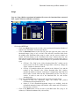
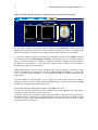
1
Functional connectivity toolbox manual v1.0
Overview
The toolbox performs seeded voxel correlations by estimating maps showing temporal
correlations between the BOLD signal from given seed and that at every brain voxel.
The toolbox implements aCompCor strategy for physiological (and other) noise source reduction,
first-level General Linear Model for correlation and regression connectivity estimation, and
second-level random-effect analyses.
The toolbox is designed to work with both resting state scans and block designs.
Installing the toolbox:
1. download conn.zip, unzip the file.
2. add ./conn/ directory to matlab path
To start the toolbox:
On the matlab prompt, type : conn
(make sure your matlab path include the path to the connectivity toolbox)
2
Functional connectivity toolbox manual v1.0
Usage
Step one: Setup (Defines experiment information, file sources for functional data, structural
data, regions of interest, and other covariates)
-
Click on the SETUP tab
o Click on the Basic button on the left side, enter experiment information (Number of
subjects, TR, and number of sessions per subject)
o Click on Functional button on the left side, from the right side panel, select the
functional images (*img, or *nii, or 4d nii). This will take a second to load, check
the middle panel (Functional data setup) to make sure the correct volumes are
loaded. The brain display in the “Functional data setup” window shows the first
(left) and last (right) scan for the selected subject/session (as in the figure above).
The current version of the toolbox assumes analyses are performed in normalized
space.
 GUI tip 1: The “Find” in the “Select functional data files” window can be
used to search for all files within the target folder recursively. Change the
“Filter” window to narrow the search.
 GUI tip 2: If multiple subjects are selected in the “Subjects” list, and the
number of files selected in the “Select functional data files” window
matches the number of subjects, each subject is assigned one single file from
the list (this is useful when one has 4-dimensional .nii files –one file per
session- in order to enter all of the functional files for each session
simultaneously)
o Click on the Structural button on the left side to load the structural images
 Option 1: load raw anatomical image, the toolbox will perform
normalization and segmentation on it.
 Option 2: If the normalized/segmented images are available, load the
normalized anatomical image (and load the white matter and CSF masks in
the next step, see below).
o Click on the ROIs button on the left side to load ROI mask files (.img or .nii
volumes) or Talairach coordinate files (.tal text files).
3
Functional connectivity toolbox manual v1.0

o
o
o
By default all files in the rois toolbox folder (./conn/rois) will be imported as
initial regions of interest. To import new ROIs, click below the last ROI
listed and enter the appropriate information.
 Load the grey matter, white matter and CSF mask for each subject if they
already exist (Option 2 in structural step above)
 Mask files should be coregistered to the normalized structural of this subject
(they could be defined in normalized space, or they could be defined in
subject-space and then transformed to normalized space in SPM).
 The default dimensions (number of PCA components to be extracted) for
each ROI can be changed here. In the following steps (preprocessing,
analyses), you can later select the number of components among the
extracted ones you wish to use in the connectivity analyses.
Click on the Conditions button on the left side to enter onsets and durations (in
seconds) of each experimental condition
Click on the Covariates:First-level button to define first level covariates such as
realignment parameters to be used in the model.
Click on the Covariates:Second-level button to define groups and subject-level
regressors (e.g. behavioral measures). Use 1/0 to define subject groups, or
continuous values to perform between-subject regression models). Click on the
empty space below “All” to add a variable.
e.g.
patients: 1 1 1 1 0 0 0 0
controls: 0 0 0 0 1 1 1 1
performance : 1 2 3 2 3 4 5 6
Note: Second-level covariates can be defined at any time in the analyses
(changes to any of other “Setup” options requires rerunning all the analyses
steps, while changes to the second-level covariates do not as they only affect the
second-level analyses in the “Results” window)
When finished defining the experiment data press Done. This will import the functional data. It
will also perform normalization & segmentation of the structural data in order to define gray
matter/ white matter/ CSF regions of interest (option 1 in structural step above). Last it will
extract the ROIs time-series (performing PCA on the within-ROI activations when appropriate).
After this process is finished come back to Setup to inspect the resulting ROIs for possible
inconsistencies. A .mat file and a folder of the same name will be created for the project.
Save / Save as button will save the setup configurations in a .mat file, which can be loaded later
(Load button). The .mat file will be updated each time the “Done” button is pressed
Note: If the data has initially been defined in SPM you can click the Import button (right after
entering the number of subjects in the Basic setup) and specify one SPM.mat file for each subject.
The program will extract the location of the functional data, the number of conditions per subject,
the onset/length of the conditions of interest, and any specified first-level covariates from these
SPM.mat files.
4
Functional connectivity toolbox manual v1.0
Step two: Preprocess (Define, explore, and remove possible confounds)
Click on the PREPROCESSING tab. By default the system will start with three different
sources of possible confounders: 1) BOLD signal from the white matter and CSF masks (5
dimensions each); 2) any previously-defined within-subject covariate (realignment parameters)
together with their first-order derivatives; and 3) the main condition effects (blocks convolved
with hrf). For each of the selected possible confounds you can change the number of dimensions
(specifying how many temporal components are being used), and the derivatives order
(specifying how many successive orders of temporal derivatives are included in the model). For
example, the realignment confound (derived from the estimated subject motion parameters) is
defined by default by 6 dimensions and 1 derivative order (indicating that the six motion
parameters are being used, in addition to their first-order temporal derivative terms). Similarly,
the White Matter confound is defined by default by 5 dimensions and 0 derivative order
(indicating that 5 PCA temporal components are being used, with not additional temporal
derivative terms).
The “Preview results” window in the right panel shows the total variance explained (r-square) by
each of the possible confounding sources (for the selected subject/session data). The dimensions
of each confound can be changed up to the values entered in the “Setup” stage, to explore its
effect on the total variance explained.
Enter the “band-pass filter” information in the bottom-left box (two numbers, in Hz, defining the
band-pass frequency window of interest).
When finished, press the Done button. This will filter the functional data and remove the effect of
the defined confounds on all brain voxels and regions of interest.
5
Functional connectivity toolbox manual v1.0
Step three: Analyze (Define and initially view the functional connectivity of different sources in
single subject level)
Click on the ANALYSES tab to define source of interest (seed ROIs).
- Use the “With-in condition weights” for the following: When estimating connectivity from
rest blocks in a more complex design (with other task blocks) between-condition differences
in activation can affect the activation at the beginning or end of the rest block. These effects
are partially controlled by entering the “condition” regressors as possible confounds. Hrf and
hanning within-condition weights attempt to further control these effects by weighting down
the initial scans within a block (hrf weights) or both the beginning and end scans within a
block (hanning weights).
- Click on “Connectivity Measures” to change the method of analysis (correlation or
regression, semipartial for multiple sources).
- The right panel (“Preview results”) displays the connectivity measures for each
subject/condition/source. Analyses here are performed in real-time (any changes in the
“Define sources” definitions affect directly the results displayed in the “Preview” window).
The measures displayed in the “Preview results” brain image correspond to the connectivity
measure selected (r if correlation is selected, beta if regression is selected). The threshold
value is also defined in the same units (in the figure above, voxels with correlation
coefficients above 0.3 are shown/colored)
When finished defining/exploring the connectivity analyses press Done. This will perform the
defined analyses for all subjects and allow the user to explore second-level (between subject)
results in the next step. First-level results (r maps or beta maps) are also exported as .nii volumes
(one per Subject/Condition/Source combination) in the results/firstlevel folder
6
Functional connectivity toolbox manual v1.0
Step four: Results (Define and explore contrasts of interest and second-level results)
At this point, second level analysis can be defined in the RESULTS window (note that
alternatively, second-level analyses can also be performed outside the toolbox, by loading the nii
images from the first level analysis into a random effects analysis program -such as SPM).
A second-level model is defined by selecting one or multiple elements in the “Subjects” list and
specifying the desired “between-subjects contrast”. For example, if we have two groups defined
(in the “covariates:second level” setup step) : patients, and controls, simply select both of them in
the “Subjects” list, and enter 1 -1 in the “Between-subject Contrast” window. This will compare
the connectivity between the two groups.
Multiple ROIs/sources can be selected simultaneously in order to analyze connectivity results
across several ROIs by specifying the contrast in “Between source contrast” (e.g. select both
“LLP” and “RLP” sources and enter a [.5 .5] contrast to estimate the average connectivity with
both sources).
The brain display at the right allows you to explore the results of the second-level analyses
estimated in real time. These results can be thresholded using a voxel-level uncorrected p-value
threshold (p<.001 uncorrected in the figure above).
When finished defining/exploring the contrasts, press Done. This will:
1) Export the defined second-level model to SPM (second-level SPM.mat, beta and contrast
volumes are saved in a folder selected by the user).
2) Produce whole brain (maximum intensity projection-MIP) results that can be interactively
thresholded using a combination of height thresholds (based on uncorrected or FDR-corrected
voxel-level p-values), and extent thresholds (based on uncorrected, FWE-corrected, or FDRcorrected cluster-level p-values).
7
Functional connectivity toolbox manual v1.0
This MIP display shows the results of the second-level analyses thresholded by a combination of
height (voxel-level) and extent (cluster-level) thresholds. Clusters are listed below together with
their peak-voxel location (in mm), number of voxels (k), uncorrected, FWE-corrected, and FDRcorrected cluster-level p- values, and uncorrected and FDR-corrected voxel-level p-values of the
peak voxel. Statistics are one-sided, select “negative contrast” in the dropdown menu at the top
right to view the results for the reverse directionality of the contrast. You can also export the
results as a text file containing the significant clusters and their statistics (“export stats”), or as a
.nii mask file defining voxels that pass the significance threshold chosen (“export mask”).