1
Quick Start Guide for Maestro2 with 2.8 Software
MD15528 Rev. B, September 2008
Acquire Fluorescence Images
This guide presumes that the Maestro 2 In-Vivo Imaging System is properly installed and
configured.
1.
Switch ON the system and the computer. Make sure the focus knob is connected, and check
that its outer rim glows with blue light. This indicates it is active and ready to use. If the blue
lights are not on, double-click the 3D Connexion Control Panel icon on the desktop to start the
device driver. You may now launch the Maestro 2 software.
2.
Push and hold the EXCITATION LAMP button for three seconds to switch on the excitation lamp.
Push the INTERIOR ILLUMINATION button to switch on the interior white lights. (These buttons
illuminate green to indicate the lights are on.)
3.
Open the specimen chamber door and place your prepared specimen at the center of the
stage.
4.
In the Maestro application, select the Acquire > Fluorescence tab.
5.
If you don’t see the Live Stream window, click the Live button to see live streaming video of the
image.
6.
In the Filter/Wavelength Selection group, select a filter set that has a wavelength range
corresponding to the fluorophore being used in your specimen. If you don’t find a preset that
works for your fluorophore/specimen, you can edit the Start, Step, and End settings manually.
Refer to the “Maestro User’s Manual” for instructions.
7.
If you want to use the filter set’s narrower band width, select the Narrow check box. Again,
refer to the “Maestro User’s Manual” for instructions.
8.
In the Wavelength And Exposure group, click the Autoexpose Mono button or enter the wavelength
at which you expect to see an image of your specimen. This should be within the range of the
current filter/wavelength selection. (Use 500 nm or above for focusing).
9.
Use the Focus knob or slider to get a sharp image of your specimen. If necessary, open the
door and adjust the position of the specimen. Close the door.
10. Select Binning, Sample Size (Zoom), and ROI (Region of Interest) options according to the
desired image quality. The default is full-field and 2x2 binning. Selecting a smaller sample
area increases the zoom. Image files will be smaller with smaller ROI and increased binning.
Binning increases sensitivity to light but reduces image resolution.
11. Click the Autoexpose Mono button again, and adjust the focus, if needed to improve the live
image.
12. Switch OFF all interior lights. (Clearing the Turn On Illumination check box will turn off the lights.)
OPEN the excitation light shutter to illuminate the specimen with the excitation light.
13. Click the Autoexpose Cube button to automatically calculate the exposure settings for the
image cube. You can also adjust the exposure time manually:
a. If the image is too dark, increase the exposure time in the Exposure (ms) box.
b. If the image is too bright or saturated (indicated by solid red pixels), reduce the exposure
time.
14. Click the Acquire Cube button to acquire a cube using the selected wavelength range. (If you
prefer to take a grayscale snapshot of the image at the current wavelength, click the Acquire
Mono button instead.)
15. When cube acquisition is complete, a color representation of the cube displays in the image
viewing area.
16. Click the Save Cube toolbar icon to save the cube. Select a location and enter a file name. (File
name format suggestion: project_sample_operator_ datetime).
17. Select a cube type option:
a. Image Cubes saves the cube in CRi format, which includes hardware and display settings
for the cube.
b. TIFF Cubes saves the cube as a series of TIFF images with the assigned file name plus an
appended number indicating the wavelength for each image in the cube.
18. Unmix the cube as explained on the next page.
CRi, 35-B Cabot Road, Woburn, MA, 01801, USA :: (Toll-Free US) 1-800-383-7924, (P) +1-781-935-9099, (F) +1-781-935-3388 :: [email protected] :: www.cri-inc.com
Quick Start Guide for Maestro2 with 2.8 Software
MD15528 Rev. B, September 2008
1.
Select the Spectra tab.
2.
If a cube is already open, it displays in the image viewing
area. To open a cube, click the Load Cube toolbar icon.
Cube format types include CRi format (*.im3) cubes and
TIFF (*.tif) cubes.
3.
The sample used in this tutorial is included with the
Maestro software and is located in the following sample
data folder: C:\Maestro Data\Images\Sample Data\Q dot
mouse stack.
4.
If a Live Stream window is still open, you may close it by
clicking its Close
box.
5.
If desired, select a spectral display option from the
Scaling drop down box.
6.
Click the Real Component Analysis (RCA) button near the
bottom of the Spectral Processing panel. The RCA function
automatically detects and separates each of the
component signals in the cube.
Unmix Images
If you prefer to unmix the cube by manually identifying
the component signals, populate the color library with
spectra and click the Manual Compute Spectra button.
Refer to the “Maestro User’s Manual” for instructions.
7.
In the RCA dialog box, you have the option of manually
sampling the autofluorescence. Click the Sample Spectrum
button and use the mouse pointer to draw a sampling line
on an area of the specimen that contains only
autofluorescence (the mouse on the right). Hold down the
left mouse button and drag the pointer to draw.
8.
Click the Find Component Images button. Maestro identifies
and displays the autofluorescence and fluorescence
signals.
9.
Select the signals you want to unmix:
a. The autofluorescence is displayed in the upper left
image. Click two times anywhere in the image to select
it as the autofluorescence. Set its pseudo color to white.
b. Single-click on the other component image(s) you want
to unmix, and select a pseudo color for each.
10. Extract the pure fluorescence signal(s) from the
autofluorescence by clicking the Find Spectra button. The
component signals display in the spectral graph.
11. Use the controls in the Computed Spectra group to specify each spectrum’s name, pseudo
color, and location within the Spectral Library.
12. When finished, click the Transfer to Library, Unmix and Close button. This adds the spectra to
the Spectral Library and unmixes the spectra in the cube. (If a library is open already, you
may be asked if you want to overwrite the existing spectra.)
13. New images will display in the image viewing area:
a. There is a small component image for each selected spectrum, each with a colored
border that corresponds to the pseudo color of that spectrum.
b. There is also a larger pseudo-colored composite image displayed to the right of the
original RGB image of the cube. The colors used to create this image are the pseudo
colors selected in the library. The result should be a clear display of the specific
fluorescence signal, with obvious differentiation from the autofluorescence.
Occasionally, for weak signals, there may be too much baseline offset in the data. If you did
not get the desired results (i.e., a clear unmixed image), repeat the RCA process and select
the Fit Offset option. Unmix again and see if the results improve.
14. Save the resulting images:
a. You can save all images as displayed by selecting File > Save Image > Save All (As Displayed). Select or create a folder in the same directory as the original image cube.
Images are saved as TIFF images that can be
opened in a variety of image display programs.
b. You can save all images as unscaled data by
selecting File > Save Image > Save All Images (As
Unscaled Data). See the “Maestro User’s
Manual” for more about saving cubes and
images.
c. You can also save the entire workspace by
selecting File > Save Result Set. Enter a file name
to save all images and results in a single file.
15. Save the Protocol and/or Spectral Library for use
throughout your experiment:
a. You can save the complete Maestro protocol,
which includes the current Spectral Library, by
selecting File > Save Protocol.
b. If you want to save the Spectral Library as a
separate file, select File > Save Spectral Library.
CRi, 35-B Cabot Road, Woburn, MA, 01801, USA :: (Toll-Free US) 1-800-383-7924, (P) +1-781-935-9099, (F) +1-781-935-3388 :: [email protected] :: www.cri-inc.com
Quick Start Guide for Maestro2 with 2.8 Software
MD15528 Rev. B, September 2008
Acquire Low-Light Images
Maestro Flex imaging systems can capture and create low-light composite images that
you can view and analyze in much the same way you would a fluorescent image cube.
This is done by first taking an image under white lights and then taking an image in
complete darkness. The system then combines these two images into a composite. For
this example of low-light acquisition, a watch with phosphorescent material on its dials
and at each hour position was used.
1.
Place your specimen on the stage and close the chamber door.
2.
Switch to the Acquire > Low Light panel. The system automatically turns off the
excitation light, closes the shutter, and switches to the Low Light filter set. (The Low
Light filter set blocks the excitation light, uses a clear emission filter, and has the
LCTF out of the light path.)
3.
The system then autoexposes the Live image with the interior illumination (white)
lights on.
4.
Click the Live button if you don’t already see the Live window. Maximize this
window, if desired, to make it easier to reposition the specimen. Fine-tune the
focus using the Focus slider or a USB-attached focus knob.
5.
Set the Binning, Max Sample Size (zoom), and ROI for this acquisition. In the figure
below, the image is zoomed to a max sample size of 1.5”x2.0.”
6.
Make sure the chamber door is closed and click the Acquire Image button. The
system will acquire a Posing Image that will act as a background for the composite
image. The system then acquires a Low Light image. Three images will display, as
shown below (you might need to press Ctrl+L to view all three images.)
•
•
•
Low Light Image (lower left)
Low Light Pose (second from left)
Low Light Composite (upper right)
7.
If the acquired images are too dark or too bright, adjust the low-light Exposure value
accordingly, and then acquire the images again.
8.
Use the measurement tools on the Measure panel (described on the back of this
page) to draw and compare measurement regions.
CRi, 35-B Cabot Road, Woburn, MA, 01801, USA :: (Toll-Free US) 1-800-383-7924, (P) +1-781-935-9099, (F) +1-781-935-3388 :: [email protected] :: www.cri-inc.com
Quick Start Guide for Maestro2 with 2.8 Software
MD15528 Rev. B, September 2008
Working With Low-Light Images
Quantifying Low Light Images
1.
Switch to the Measure panel and maximize the Low Light Image window.
2.
You can use the Auto Calculate Threshold feature or manually draw
regions around regions of interest. For this example, Auto Calculate
Threshold was used and then the Threshold Level was decreased until
regions were drawn around all of the luminescent areas, as shown in
this example.
3.
By clicking the Grow button at the far right of the Measurements data tab,
you can easily compare the Average Signal, Total Signal, and other
measurement data for all of the regions.
Enhancing Low-Light Images
1.
Enhance the display of your low-light images by using the Display Control tool.
2.
Maximize the Low Light Composite image first, then click the Display Control button on the
toolbar.
3.
Adjust the Contrast, Gamma, and Brightness sliders to achieve the desired display of your
image. You can also use the other display control features to enhance the composite display.
(Refer also to the Maestro User’s Manual for more about the Display Control tool.)
Saving Low-Light Images
To Save the Composite:
If you want to save images in a single composite.imx file (includes the low-light pose, low-light
image, and low-light composite), select the composite image and select File > Save Composite from
the menu. Enter a Composite Image File name and click Save.
To save Images as Unscaled Data:
If you want to save each image as a separate file and preserve its data for later quantitative
analysis, select File > Save All Images (As Unscaled Data). You will be prompted to name and save
each file separately.
CRi, 35-B Cabot Road, Woburn, MA, 01801, USA :: (Toll-Free US) 1-800-383-7924, (P) +1-781-935-9099, (F) +1-781-935-3388 :: [email protected] :: www.cri-inc.com
Quick Start Guide for Maestro2 with 2.8 Software
MD15528 Rev. B, September 2008
Dynamic Contrast Enhancement
Dynamic Contrast Enhancement (DyCE) is a plugin application that can be purchased as an add-on to your
Maestro system. DyCE is a simple, inexpensive and versatile new approach that can provide coregistered
anatomical information by exploiting in vivo pharmacokinetics of dyes in small animals. (A detailed
explanation of DyCE technology is available in the Maestro 2 User’s Manual.)
Preparing for DyCE Imaging
System Setup:
1.
Make sure the Maestro system is turned on and the Hardware Status indicator
in the software displays “Ready.”
2.
Make sure the multiview platform (if purchased) is installed and connected to
the interface and anesthesia ports inside the chamber.
3.
Make sure the Live Stream window is displayed (click the Live button if it is not).
4.
On the Acquire > Fluorescence tab, select camera settings, a filter set, and any
other acquisition parameters. Or if a protocol has been saved for this application,
then load the saved protocol.
5.
Make sure the appropriate lights within the chamber are turned
on and the platform is heated to the proper temperature. Ideal
lighting conditions depend on the dye or agent that will be used
during the current application.
6.
In the Maestro software, click the Acquire DyCE button or select
Tools > Acquire DyCE from the main menu. If you have not yet
activated the DyCE plugin, select DyCE Limited Time Trial from the
Tools menu. Enter your activation code if you purshased a
license to use DyCE. If you have not yet purchased a license,
you may evaluate DyCE for up to 30 days.
7.
The Acquire Dyce window (see Figure at right) will open with its
Acquire tab displayed.
Selecting Binning and ROI:
1.
Select the desired Binning and ROI for this acquisition. The Total
Time displays the current estimate of the time required to acquire
the dataset using the currently selected Time Series.
2.
Check the estimated data size of the dataset when acquired. It is important to keep
this value below 150 megabytes due to memory limitations; datasets that are larger
than 150 MB may be too large to analyze. The value displays in green to indicate an
acceptable file size. Red indicates that the file may be too large at the current
settings. (Increasing the binning or choosing a smaller ROI will decrease the
estimated size of the dataset.)
3.
In the Save Options box, click the Browse button to
navigate to the directory where you want to save the
acquired dataset. Select a location, then name the
dataset in the Cube Name box.
4.
Place the anesthetized mouse on the platform Be
careful not to touch or smudge the mirrors on the
platform while placing the mouse. Make sure the
mouse’s nose fits snug in the anesthesia nosecone.
5.
Prepare for the bolus injection: So that you do not have
to open the chamber door to give the injection, use one
of the utility ports on the side of the system instead. A
catheter inserted through a utility port and then into the
rodent’s tail will make it much easier to give the injection.
Otherwise, you will have to open the door, give the
injection, and immediately close the door before clicking
the Acquire button.
6.
Click Autoexpose to calculate optimum exposure settings.
7.
When ready, give the injection and click Acquire to collect
the series of images over the specified time intervals.
8.
The acquired images are compiled into an RGB cube. If
you selected the Launch Viewer After Acquire check box,
the cube will display in the DyCE Explorer window as
well as in the Maestro window.
Selecting a Collection Type:
The Collection Type determines the type of dataset that will be collected. There are three
options:
•
Mono (broadband emission) acquires a monochrome image at the selected time
intervals with the tunable filter out of the light path.
•
Mono (using current Acquire wavelength) acquires a monochrome image at the
selected time intervals with the tunable filter in the light path.
•
Cub (using current Acquire settings) collects a series of complete multispectral cubes
for the duration of the selected time interval.
Selecting Save Options:
Select a directory/folder where you would like to save the acquired dataset(s). Enter a
base cube name in the Cube Name field.
Acquiring a Monochrome DyCE Dataset
1.
Select Mono (broadband emission) or Mono (using current Acquire wavelength) as the
collection type. Both of these options let you configure up to three collection intervals,
which gives you the ability to set a different frame rate for each interval. This is
important because in most cases you want to capture more frames (i.e., more data)
during the first few seconds immediately following the bolus injection.
2.
Configure the Time Series: For example, as shown in the example above, you might
want to capture 5 frames per second for the first 25 seconds, with an exposure time
of 221 ms per frame. The next 10 seconds will capture 2 frames per second. During
the final 5 seconds, the system will capture just 1 frame per second.
CRi, 35-B Cabot Road, Woburn, MA, 01801, USA :: (Toll-Free US) 1-800-383-7924, (P) +1-781-935-9099, (F) +1-781-935-3388 :: [email protected] :: www.cri-inc.com
Quick Start Guide for Maestro2 with 2.8 Software
MD15528 Rev. B, September 2008
Acquiring a Multispectral DyCE Dataset
1.
2.
Select Cube (using current Acquire settings) as the collection type. This option lets you
acquire a time series of complete multispectral cubes following a bolus injection. Up to
three intervals may be collected. These intervals let you control the sample rate (frame
rate) and exposure time. The system will use the cube acquisition settings currently
selected on the Acquire panel.
For example, for the first 20 seconds
immediately following injection, you
might want to collect a multispectral
cube every 5 seconds. Then for the
next 2 minutes, collect one cube
every 30 seconds. During a third
interval, you might collect one cube
every minute for 5 minutes. The
example here demonstrates these
time series settings.
Note: When collecting cubes, the
values in the Frame Rate selectors are timers that control the number of seconds that
are allowed to lapse between the start of each cube during that interval. Always set the
Frame Rate Unit to “Sec./Frame” (think of it as “Seconds per Cube”) for cube collection.
To create a new DyCE time series from a sequence of
cubes:
1.
When a Cube time series acquisition is complete, the
Create from Cube Sequence functions become enabled.
2.
Select any cube from the Cubes drop down box. The
cube will open in the DyCE Explorer and in the
Maestro software. Try to find the cube that best
displays the spectral component you want to use to
create the DyCE time series.
3.
In Maestro, switch to the Spectra panel. Use the Library
color palette to sample the spectral component you
want to obtain from each cube in the dataset. The ID
of the spectra will be added to the Component To Keep
drop down box.
3.
Select an exposure setting for each time interval. This value overrides any cube
autoexposures done via the Acquire panel.
4.
Select the component to keep from the drop down
box.
4.
In the Save Options box, click the Browse button to navigate to the directory where you
want to save the acquired sequence of cubes. Select a location, then enter a base
name for the cubes in the Cube Name box.
5.
5.
Place the mouse on the platform and acquire the DyCE images as described on the
previous page. If you selected the Launch Viewer After Acquire check box in the Acquire
window, the first cube in the sequence displays in the DyCE Explorer and in Maestro.
Click the Create DyCE Time Series button. The Maestro
software will open each cube in the sequence and
obtain the selected component from each of them.
The software will then compile all of these signals into
a new cube file.
Reviewing DyCE Datasets
If the dataset is not open in Maestro already, load it now by clicking the Load Cube button.
Then select Tools > DyCE Explorer from the Maestro menu. Click the Play button.
The Play bar indicates the current frame and the total number of frames. You can drag this
bar or use the scroll box to freeze any individual frame. The frame number and wavelength
display in the bottom-right corner. The vertical blue line on the Plot graph indicates the time
of the current frame. Also, you can move the mouse pointer over the displayed image to plot
the spectral curve of the pixels at the cursor location (shown by the dotted grey line).
Changing the Display Mapping
Two sliders let you adjust the brightness and contrast of the display image. All display
changes effect the entire dataset, not just the current frame (middle-right image).
Min. Max. maps the minimum value in the entire sequence to 0, the maximum value to 255,
and linearly interpolates in between those values. This stretches dark signals so they
become visible.
Clip/Stretch maps the lowest 0.01% of the pixels in the entire sequence to 0, the highest
0.01% to 255, and linearly interpolates in between those values. This prevents a few bright
or saturated pixels from skewing the display.
Histogram Eq. maps the pixels in the entire sequence so the histogram of the pixels have
approximately the same number of pixels in each bin. This gives the best display of the
whole dynamic range of dim and bright signals.
You can assign specific minimum and maximum clip values to the display of the image.
Increase the Min Clip value to exclude more of the lowest value pixels from the display.
Decrease the Max Clip value to exclude more of the highest value pixels.
You can also select a Color Map depending on the brightness and contrast of the image and
the type of dye or agent you are trying to visualize in the movie.
Displaying Dimension-Reduced Data
Saving Images and Movies
You don’t have to view the individual planes in a dataset one frame at a time. The DyCE
Explorer can identify the strongest signals in the sequence and combine them in a
transparent “flattened” image. Check the Display Dimension-Reduced Data box to reveal a new
multicolor representation of the data (bottom-right image).
If you want to save the current frame as it is currently
displayed, right-click over the image and select an option
from the pop-up menu. You can save the image (i.e., frame)
as displayed as a TIF or JPG image, or copy the current
frame to the clipboard.
Initially, all of the planes in the DyCE sequence will be reduced to just three planes. These
planes will be different linear combinations of all the planes in the sequence. Change the
number of dimensions (i.e., anatomical signatures) by scrolling the Dimensions box.
Clicking the Save button saves the dataset as an AVI movie
file. AVI movie players can now play your DyCE movie.
CRi, 35-B Cabot Road, Woburn, MA, 01801, USA :: (Toll-Free US) 1-800-383-7924, (P) +1-781-935-9099, (F) +1-781-935-3388 :: [email protected] :: www.cri-inc.com