Download User Guide to 1.5-m Fiber Echelle Spectrograph

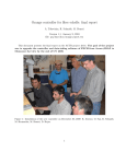
Cerro Tololo Inter-American Observatory
User Guide to 1.5-m Fiber Echelle Spectrograph
A. Tokovinin
Version 3. April 29, 2010 (ech manual.pdf)
1
1
Instrument description
The echelle spectrograph was used at the Blanco telescope and now, after having been de-commissioned,
it is located in the coudé room of the 1.5-m telescope and connected to it by optical fiber. The FrontEnd Module (FEM) matches the fiber to the telescope and provides for auxiliary functions such as
guiding and comparison spectra. The Back-End Module (BEM) couples the fiber with the spectrograph and permits inserting the iodine cell in the beam.
1.1
Interface to the GAM
78mm
to top plate
To GAM CCD
To FEM
Probe position:
X=−368, Y=+259
Figure 1: M1 mirror attached to the GAM probe.
The Guiding and Acquisition Module (GAM) is normally used for offset guiding. It has been
modified by adding a piggy-back mirror M1 on top of the guide probe (Fig. 1). Positioning this
probe at the center of the field (X=−268, Y=+259) makes M1 to intercept the on-axis beam without
vignetting and to direct it sideways, to the FEM which is attached to the GAM hatch door. The
optical axis of the beam deflected by M1 is at 78 mm below the lower surface of the GAM top plate.
Normal operation of the probe is not perturbed, it captures the field at a fixed offset and, if we
are lucky to find guide stars there, the standard guiding is possible. The object would be centered in
the GAM-camera field if we set Y=-96, but then FEM receives no light.
1.2
FEM and its connections
Figure 2 shows the FEM attached to the GAM. The space is restricted from all sides. To remove the
FEM, loosen the 4 M4 screws, turn the FEM anti-clockwise and pull it away, leaving the screws in
place. Be careful not to damage the cables and the optical fiber! Installation – in the reverse order.
The FEM is permanently installed on the telescope, but any repair or trouble-shooting require its
removal because accessing it is difficult.
2
Alignment check
To Comp.
sources
Fiber cable
Pins
CCD camera
To electronics
box
Figure 2: FEM attached to the GAM door (views from two sides).
Light
Electronics
To control room
Ethernet
Telescope
Electronics Switch
M1 mirror in the GAM
GAM
FEM
CCD
Main fiber cable
Comp. light
fiber
Gigabit Ethernet
BEM
Coude room
PC 139.229.12.62
Guider
GUI
CCD
Spectrograph
PC 139.229.12.29
Temperature
controler
Monitor (VNC connection)
Computer room
Control room
Fiber
Monsoon CCD controller
Figure 3: Connections of the 1.5-m echelle system.
The main fiber cable can be detached from the FEM. Its exact position is critical, it is defined by
two pins. Be careful not to damage them! The optical alignment between the fiber and the hole must
be checked each after time the cable was detached. Do not detach the fiber cable unless it is really
necessary.
The connections of FEM are shown in Fig. 3. The orange fiber cable brings the light of the
comparison sources, it is permanently fixed inside the FEM (to detach it, the FEM must be opened).
3
M2
Comparison light
Prism
M3
M2
Fiber
cable
holder
"Bench"
Motor
From GAM
Guider CCD
Figure 4: Schematic representation of the mechanical design of the front-end module.
The comparison source module (“light box”) is mounted at the telescope jointly with the electronics
box which powers the light sources (thorium-argon lamp and quartz lamp). The electronic box connects
to FEM with a short cable and to the control room with the ethernet cable (and, additionally, by
a cable that goes through the J27 round connector on the telescope and is used for manual control
of the lamps). The guiding CCD camera is powered from the electronics box through FEM (a short
cable, +12V), while its digital signal is sent to the guiding PC in the computer room by a dedicated
Gigabit Ethernet cable.
1.3
What is inside FEM?
The main components of FEM are shown in Fig. 4. The incoming beam is focused on the concave
mirror M2 with two holes in it, one for the star and another, larger – for the sky (not used). The light
which goes through the central hole is transformed from F/7.5 to F/5 by a pair of small lenses and is
injected into the fiber with a core diameter 100 micron.
The co-alignment between the hole and the fiber is very important. To check it easily, an auxiliary
optics (a small mirror and a strong eyepiece) can be lowered in front of M2 (“Alignment check” in
Fig. 2). The back-end of the fiber is illuminated (put paper on the slit, turn on the light in the coude
room), and the image of its front end can be seen through the hole and centered (by tiny motions in
the fiber holder). Do not forget to retract the auxiliary optics after the alignment check!
The light which does not pass through the hole is reflected by M2, then directed by a flat mirror
M3 to the optics of the guider. The 3x reduced image of the field (i.e. of M2) is formed on the CCD
camera GC650 from Prosilica. The digidat signal is sent via Ethernet cable to the guiding PC (see
below).
The light of the comparison lamps is directed into the main fiber by moving a small (2-mm) prism
which slides behind M2. The prism is pushed by a cam mechanism which, in turn, is actuated by a
small servo motor.
4
1.4
Light box and electronics
M2
Quartz lamp
Filter
Fiber end
Th−Ar lamp
M1 L
Figure 5: Optical scheme and picture of the Light Box.
The light box contains the thorium-argon spectral lamp and the quartz lamp. The SMA connector
of the fiber (core diameter 0.4 mm) receives the image of the thorium cathode formed by a F = 18 mm
lens (it is aligned with the fiber). The lamp is powered by 500 V voltage produced by the DC/DC
converter in the light box, while a 50 kOhm/12W resistor in series limits its current to 8 ma. The
life time of this lamp is short (500 hours), so it should be switched on only during comparison
exposures.
The quartz lamp (5V, 10W) is also co-aligned with the fiber, so its light is very bright. The 4-mm
thick BG38 color-balance filter is installed to equalize the intensity between red and blue wavelengths.
This lamp serves for flat-fielding the spectra.
The electronics box contains a simple pulse generator for controlling the prism servo motor in
the FEM, relays for switching the spectral lamps, logic, and the power supplies (12V and 5V). The
DC/DC converter for the spectral lamp is powered by 12 V. The power switch on this box activates
all the electronics. Please, switch off the electronics at the end of the night.
The control of the lamps, motor, and LED done by the data-taking software. In addition, there is
a small box in the control room for manual operation. It has a switch with 3 positions. In the central
(neutral) position the prism is retracted, starlight enters the spectrograph. In the left position, the
prism is “In”, the Th-Ar lamp is on, and the red LED is illuminated. In the right position, the Quartz
lamp is on, with yellow LED illuminated.
1.5
Acquisition and guiding
The guiding camera is GC650 from Prosilica. It has 659x493 square pixels, pixel size 7.4 micron
(0.38 arcsec on the sky), field of view 3 arcmin. diameter. The signal depth is 14 bits (4096 counts).
Minimum exposure time is 0.000001s (10 microseconds). The camera is powered by +12 V from FEM.
Its digital signal is transmitted by a dedicated Ethernet cable to the guiding PC which is rack-mounted
in the computer room. This PC runs under Linux, its name is ctioxb, fixed IP adress: 139.229.12.62.
The standard PCguider program runs on this computer (Fig. 6).
After turning on the electronic box (hence the camera), enter the guiding program by VNC connection from a suitable terminal: vncviewer 139.229.12.62:1. In the VNC screen, open the PCguider
from a menu activated by the left mouse button. In order to see better star images, use automatic
5
Figure 6: Snapshot of the PCguider screen during guiding.
intensity scaling (this is a new program feature). To do so, use menu in PCguider: Options →
Parameters → olut = off (the default is sigma).
When the field is illuminated by sky or dome light, dark images of the two holes are seen. The
guiding box should be centered on the small hole, normally at X=289, Y=255. You may want to shift
the box by ±1 pixel to achieve better centering of the star in the hole. The normal box size is 29
pixels. The North-South direction coincides with Y.
After pointing the telescope, the object should be seen on the screen. Adjust camera integration
time to avoid saturation (max. counts < 4096). In the PCguider menu, use Windows → Camera
Control → Integration Time, set the new value, press Enter. The effect is immediate. In Fig. 6,
the integration time is 100 ms.
Using hand paddle, move the telescope to bring the star into the box. Most of the image disappears
in the hole, and we see a ring (donut), as shown in Fig. 6. The guiding loop can now be closed. To
view the image better, adjust the display using its control panel (display menu: Options → Control
panel). It is helpful to adjust the contrast and brightness and to use zoom for a larger view of star
image in the hole.
For focusing the telescope, move the star away from the hole, make sure that the image is not saturated in the camera (max. count < 4096) and in the display. With bad settings of brightness/contrast,
the central part of the image looks “flat”, with right settings it is peaked.
6
The position of the guider arm must be checked because the GAM control software systematically
goes wrong, so the displayed coordinates of the guide arm do not match its actual position. The
correct position should be X = −268, Y = +259, Z = −41. Put a bright star away from the hole,
defocus the telescope, and verify that the image is ring-like, not cut on one side. If this is not the
case, re-initialize the GAM control program and set the GAM probe again where it should be.
2
2.1
The spectrograph
Back-end module
Fiber
M3
Y
X
Focus
Slit
Figure 7: Back-End Module at the spectrograph. Left: without the iodine cell, right: with the cell in
the “out” position.
The Back-End Module (BEM) is mounted on the front plate of the Blanco Echelle Spectrograph by
means of the AR90 angular bracket, attached to the plate with two 1/4 screws (Fig. 7). The bracket
holds the rail with two carriages. The upper carriage holds the 50-mm focus lens and the fiber cable
termination. The cable must be inserted and fixed by tightening the M3 set screw. This assembly is
pre-aligned to give a parallel and well-centered beam. The diameter of the emerging collimated beam
is about 10 mm.
The lower carriage holds the 75-mm focus lens which re-focuses the fiber-end image on the slit.
The magnification is 1.5x, so the image diameter is 150 µm. The slit is ∼42 mm below the surface
of the front plate, its orientation is indicated in Fig. 7. The X and Y knobs permit to move the
fiber image on the slit in, respectively, perpendicular and parallel directions. The image is focused by
moving the whole lower carriage along the rail.
7
With the fiber illuminated (sky through the telescope or quartz lamp), the image of the fiber is
focused and centered on the slit by looking in the post-slit viewer. Initially the slit is wide, then it is
set to the desired width (between 60 µm and 150 µm), with the smallest decker.
2.2
Spectrograph setting and focus
The echelle grating is 31.6 l/mm, the cross-disperser is number-3, 226 l/mm. The angle of the echelle
is 568, set to center the blaze function on the detector. Fig. 9 shows that this centering is good. The
collimator focus is 99.80. The cross-disperser angle is set to 1114. These settings must never be
changed!
Figure 8: Correspondence between wavelength and line number (Y) for the current spectrograph
setting (full-frame readout).
The correspondence between the vertical coordinate on the CCD and the wavelength (in Å) is
plotted in Fig. 8. It is well approximated by second-order polynomials:
λ = 4023.47 + 1.6599Y − 1.98 10−5 Y 2
Y
= −3.06 + 0.602L + 3.4 10
−6 2
L ,
L = λ − 4000.
(1)
(2)
The full coverage is from 4020Å to 7300Å. The iodine setup (Y from 400 to 1600) corresponds to the
wavelengths from 4670Å to 6650Å.
The fiber image is projected onto the slit with 1.5x magnification. The actual slit width is about
40 µm larger than the micrometer reading, as deduced from the transmission measurements (Fig. 10).
For high-resolution work, we recommend the micrometer setting of 50 µm (actual slit width 90 µm)
which gives R = 43 000 at the expense of 70% transmission. For faint stars, open the micrometer to
100 µm to transmit the full fiber image.
The Schmidt camera of the spectrograph has no field flattener, so the focal surface has a curvature
radius of about 590 mm, with a convex side pointing to the camera. It is not possible to adjust
the detector tilt and focus for the whole field simultaneously. These parameters are controlled by
taking thorium exposures with two masks, “west” and “east”, and finding the relative X-displacement
between the matching lines in both images automatically (with focus.pro in IDL). The detector tilt
was adjusted so that the center of the curved focal surface is near the detector center. Figure 11
shows the iso-focal lines, with the inner contour corresponding to the perfect focus. The dewar focus
8
Figure 9: Plots of the extracted spectra of HR 4546 around Hα (left – the whole order, right – zoom on
Hα). The spectrum has not been flat-fielded, the difference in the response between the two amplifiers
(left and right halves) is apparent.
Figure 10: Slit transmission versus
micrometer reading. The points are
measurements with Quartz lamp,
the curve is the analytic
model t =
p
1−(2/π)(acos β −β 1 − β 2 ), where
β is the ratio of slit width to fiber
diameter.
position is 1.00 mm, so that the CCD is slightly (by 0.1 mm) beyond the best focus at the center of
the field (positive defocus in Fig. 11), to offset partially the field curvature.
Figure 11: Contour plot of the spectrograph focus after final adjustment (May 23, 2008). The
CCD lines from 400 to 1599 are read out (iodine
setup), so the Y-center is at line 1000. The defocus at the center is +0.093 mm (CCD behind the
focus), the curvature radius of the focal surface
is ∼ 0.5 m, concave to the detector.
9
Ethernet
ADAM
Linux PC
Ethernet
systran fiber
Temperature,
I2 cell control
Dewar
RS−232
Coude room
Computer
room
shutter
Monsoon Orange
Telescope
ADAM
+5V
Prism and
comparison lamps
Power−supply
Lakeshore
box
Figure 12: Elements of the new controller system and their connections.
2.3
Iodine cell
The iodine cell is a glass cylinder (50 mm diameter, 100 mm length) wrapped in a heater tape. The
temperature controller maintains the cell at 55◦ C (there is a sensor below the heater tape). When
switched on, the controller can “over-shoot” and heats the cell well above the desired temperature.
This must be avoided by watching the temperature. If it is over-shooting, push the “Stop” button on
the controller, watch the temperature to go below the set point, then push “Run” again. The cell is
housed in a small black container which can be inserted manually in the parallel beam of the BEM,
being mounted on the hinge. This motion will be motorized. A new container/heater combination has
been fabricated in January 2010, but it is not in use now. In the near future, the in-out cell motion
will be remotely controlled.
2.4
CCD and data acquisition
The CCD is a 2048x2048 SITe chip with 24-micron pixels. It is housed in the CTIO SITe 6 dewar
and works with the Monsoon Orange controller (it replaced the old Arcon controller in January 2010).
The new controller consists of several inter-connected modules (Fig. 12).
We use the readout with two “upper” amplifiers (UL,UR). The gain and full-chip readout time can
be optimized by selecting fast mode for bright stars or normal mode for faint stars (Table 1). When
only 1/2 of the chip is read out (iodine-cell observations), the fast readout takes about 10 s. The CCD
is not yet saturated at the maximum count, 65 000 ADU (to be checked).
10
Table 1: Readout modes and parameters
Parameter
Readout time, s
Gain e-/ADU
RON, ADU
RON, electrons
Fast mode
UL UR
18
3.3
3.0
2.8
3.3
9.2
9.9
Normal mode
UL
UR
27
0.91
0.81
8.0
8.2
7.3
6.6
Figure 13: Detected flux near 550 nm (electrons per pixel per second, summed across order) vs. star
magnitude. The dotted line shows 1% total efficiency.
2.5
System efficiency
The overall efficiency (the number of detected photons relative to the number of incident photons
outside atmosphere) is estimated at 1% with a 60-micron slit transmitting 60% of light (Fig. 13). A
V = 5m star gives flux of 116 el/pixel/s. The width of the orders in the cross-dispersion direction is
about 3.8 pixels, so the flux per pixel in the 2-dimensional frames is ∼ 3.8 times less than the integrated
flux. A S/N=100 will be reached on a V = 7m star in a 10-min. exposure. Some stars show a reduced
efficiency, presumably due to clouds, poor guiding, or bad seeing. Efficiency of 1.7% is expected with
the fully opened 150-micron slit, giving spectral resolution R ∼ 25000. For comparison, other echelle
spectrographs have efficiency 7% (Hamilton, HARPS), 12% (HIRES), or even 15% (FEROS).
3
Check-list
The checks listed below should be made each time the instrument is installed at the telescope or
modified. Some of these checks may be useful for trouble-shooting.
• Verify all connections (Fig. 3).
11
• Electronics functionality. Move the prism in and out and hear the motor moving through the
microphone placed near the FEM. Switch on quartz or Th-Ar lamps, see the light coming out
of the fiber connector on the light box.
• CCD camera functionality. The image of the field with two holes (big and small) should be seen
on the PCguider screen with the dome illuminated. Make sure this image is sharp.
• Fiber-hole co-alignment. Back-illuminate the fiber by placing a piece of white paper on the
lower BEM lens and switching on the light in the coude room. Detach FEM from the telescope
without disconnecting. On the FEM, release the fixing screw on the alignment-check optics
(Fig. 2, right), move the lever down to un-cover the hole, and see the round image of the fiber
end through the hole. In the case the image is not round (obstructed by the hole on one side),
make a very slight correction with the set-screws in the fiber holder. Be careful not to turn these
screws by more than 1/4 of the revolution and always leave them tightened.
• Spectrograph focus. Take two Th-Ar exposures with the Hartmann mask in the “West” and
“East” positions. Export the images to FITS and run focus.pro in IDL to obtain the plot like
Fig. 11. If the spectrograph is properly focused, the FWHM of unsaturated Th-Ar lines near
the center of the detector should be 1.95 pixels (slit setting 50 µm, no masks).
12