1
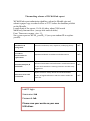
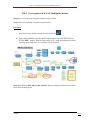
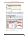
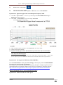
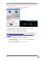
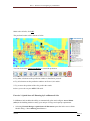
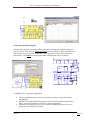
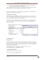
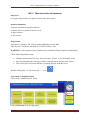
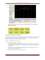
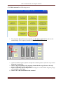
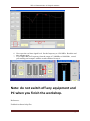
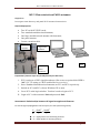
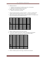
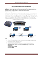
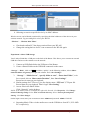
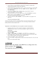
Wireless Communications and Satellite Systems Lab Manual Ya Bao Table of Contents The marking scheme of WC&SS lab report .............................................................................. 3 Lab Report Guidelines............................................................................................................... 4 WE-1 Investigation on WLAN Multipath Channel ................................................................. 5 WE-2 Radio Signal Monitoring and White Space Allocation ................................................. 8 WE-3 Wireless LAN designing by LANPlanner .................................................................. 13 WE-4 Characteristics of Antennas ........................................................................................ 21 WE-5 Characteristics of WiFi antennas ................................................................................ 29 WE-6 Optimise and secure a WiFi network.......................................................................... 34 Ya Bao Page 2 The marking scheme of WC&SS lab report WC&SS lab report submission deadline: upload to Moodle site and submit a paper copy to school office at T313 before the deadline publish on the Moodle. Length limit of the report: 10-14 A4 sides, about 3000 words Main body font and size: (except title and sub-titles) Font: Times new roman: size: 11. Save your report as WCSS_yourID_15 (use your student ID to replace yourID) Introduction & Background General introduction, aims, objectives, underlying theory 20% Procedures, Measurements & Explanations Experimental details. Procedures and observations 20% Discussion, Analysis, & Conclusions Explanation of the measured results and observations. Numerical evaluations and verifications. Conclusions based on the work carried out. Learning outcomes. Further study suggestions. 40% Report structure. Clearly written and understandable. Quality of English References and the citation within the main text. 20% References & Overall presentation Lab PC login Username: lab Password: lab Please save your works on your own USB driver. Lab Report Guidelines Formal lab reports should be typed on A4 paper and contain the following sections and don’t exceed the limit of the length. Title Page: Title of the experiment, Author’s name and student number. Your instructor's name. The date the report was submitted. Aims and objectives What was the purpose of the experiment? What was it supposed to reveal? Introduction/Theory The introduction should give some background on the problem your experiment investigated. Theory section presents theoretical models, equations, physical principles, etc., that are relevant to the investigation described in the report. It should be within one page. Materials List everything needed to complete your experiment. Methods/Procedure Describe the steps you completed during your investigation. Don’t simply copy the instructions given in the lab manual. You need to describe what YOU did. Make good use of diagrams, sketches, or photographs to show important layout, wiring and connections Experimental Results and explanations Present your results and summarise the data using figures and tables. Each figure and each table must have a number and a caption. Do not simply dump a bunch of graphs and tables into this section with no explanation. It is best to locate figures and tables within the text (and preferably on the same page where they are referred to) rather than grouping them together at the end of the report. Discussion Discuss the meaning and importance of the experimental results, compare the results to theoretical predictions, describe the accuracy of the results, address discrepancies, and ultimately draw conclusions in regards to the objectives of the experiment. Conclusions and Recommendations This section summarizes the conclusions that have been made and gives specific recommendations for the next steps that could be taken in subsequent experiments or further research. References If your research was based on someone else's work or if you cited facts that require documentation, then you should list these references. http://www.lsbu.ac.uk/library/html/documents/HS28-numeric2012.pdf is a very helpful sheet on how referencing should be done in any technical report (Lab or final project) References: 1. Dr. Sandra Dudley, Typical Lab report contents 2. BJ Furman, Laboratory Report Guidelines Ya Bao Page 4 WE-1 Investigation on WLAN Multipath Channel WE-1 Investigation on WLAN Multipath Channel Objective: to investigate the multipath channel in 802.11a PHY. Tools: MATLAB, Simulink, Communications Blockset. Procedure: 1. Start MATLAB by double-clicking the MATLAB icon 2. Type commwlan80211a at the MATLAB prompt to open the IEEE 802.11a WLAN PHY model. Then save the model as xx_wlan in the directory where you keep your work files. (xx could be your first name) Question 1. What is IEEE 802.11a WLAN PHY? Briefly explain the functions of each blue block in the model diagram. Ya Bao Page 5 WE-1 Investigation on WLAN Multipath Channel 3. Double click the Multipath Channel block; choose No Fading from Fading Mode window. Set SNR at 30 dB. Click Apply, then OK. 4. Run the model by click button on the tool bar. Record the reading of PER(%) and Bit Rate (Mb/s). 5. While the model is running, double click on the Signal Visualization block to open a real time scopes. It is really helpful for your understand of fading effects. After the simulation, you can click the Tools→Data Statistics →data 5 (SNR) or data 4 (Bit rate) or data 3 (BER). Record the mean value. (You can take the measurement after running for 1 minute then stop the running. Wait for the ending of the simulation takes time). 6. Change the setting of SNR (-5 to 35 dB) to obtain the trend of BER-SNR 7. Change the setting of SNR (-5 to 35 dB) to obtain the trend of Bit Rate-SNR. 8. Plot BER-SNR and Bit Rate-SNR graphs, respectively. Ya Bao Page 6 WE-1 Investigation on WLAN Multipath Channel SNR (dB) BER Bit rate (MBps) -5 -2 0 2 5 10 15 20 25 30 35 1. Change to Flat fading and Dispersive fading, respectively. Record and plot BER-SNR BER-Bit Rate graphs. (Because of fading, real time value is variable. You can use the mean from the Data Statistics.) Question 2: explain the terms of Fading Flat fading Dispersive fading References: MATLAB R2007b Help file Ya Bao Page 7 WE-2 Radio Signal Monitoring and White Space Allocation WE-2 Radio Signal Monitoring and White Space Allocation The electromagnetic spectrum is a continuum of all electromagnetic waves arranged according to frequency and wavelength. The signal strength (dBm) of frequencies in the range the user has specified can be monitored by the spectrum analyser. Objectives: Monitor the signal strength in the specified frequency band. Define and locate White Space Monitor Specific Frequencies Plot 3-Dimensional Heatmap Equipments: Invisible Waves RF Analyzer kit PC with software installed Initial Experiment Setup (Step 1 to 4 maybe already set.) 1) Ensure the analyser kit has been correctly connected. 2) Switch on PC, choose Windows XP, login with user name: lab and password: lab. 3) Connect the analyzer with PC via the USB cable. 4) Switch on the analyzer’s power. Step 1 to 4 maybe already set. Ya Bao Page 8 WE-2 Radio Signal Monitoring and White Space Allocation 5) Double Click on the desktop. 6) 7) Close the Control Panel::Default Click the main window, View-- Options – Hardware, choose 1700-3500 MHz Experiment 1. Signal strength of the 3G mobile phone frequency band 1.1 Click File – Open Profiles… to choose a pre defined profile 2100-2190BaseStation.iwp in RFAnalyzer folder and open it. 1.2 Click View – Control Panel, record your settings. Start Scan You should see following results. 1.3 After scanned for about 10 minutes, click Stop Scan in the control Panel. 1.4 Check and record the heatmap 1.5 Explain what RF signal carrier allocated in this spectrum? How wide of each channel? Note: Export the data and graph Move your cursor in the graph you wish to save, right click to choose Export Data..., choose Jpeg to save a file on your own USB disk to choose Text to save date which can be open in Excel. Experiment 2. Investigate the ISM band (2400-2500MHz) Use the Control Panel to change the Scan Setting to the frequency band of 2400-2500MHz. Investigate the signal strength, and heatmap. Record your observation and explain which frequency bands are in higher signal levels and what applications are using these bands. Please refer to the Frequency Allocation Table at http://www.ofcom.org.uk/static/archive/ra/topics/spectrum-strat/uk-fat/uk-fat2002.htm What is ISM band? Why we choose ISM band to study? Experiment 3. Define and allocate White spaces Ya Bao Page 9 WE-2 Radio Signal Monitoring and White Space Allocation White space is the band between used radio frequency bands. RF analyzer can find and allocate the white space in a specific range. 3.1 In the control panel, close the Sensitivity Setting and Scaling sections. 3.2 choose a White Space Threshold(dBm) at -100 3.3 Change the bandwidth setting from 2 MHz to 5 MHz, compare the observations. 3.4 Change the threshold to -110, compare the observations. Experiment 4. Investigate a wide band (1710 – 3500 MHz) Record your observation and explain which frequency bands are in higher signal levels and what wireless applications are using these bands. Please refer to the Frequency Allocation Table at http://www.ofcom.org.uk/static/archive/ra/topics/spectrum-strat/uk-fat/ukfat2002.htm Experiment 5. Monitoring 3G mobile phone signal (optional) 5.1. Click File – Open Profiles… to choose a pre defined profile 1900-2000mobile.iwp in RFAnalyzer folder and open it. 5.2. Click View – Control Panel, record your settings. Start Scan You should see following results. Ya Bao Page 10 WE-2 Radio Signal Monitoring and White Space Allocation 5.3. Explain what RF signal allocated in this spectrum? 5.4. Switch on your 3G mobile around the analyser’s antenna and start to surf the Internet while the analyser is scanning. What’s happening on your monitor? Try switch on another company’s mobile phone (if available) and common on your finding. 5.5. What company network did this mobile run on? Is it match with your SIM card? What’s about if your SIM card not belonged within above 4/5 companies? Note: Third-Generation (3G) Frequency Range: Frequency (MHz) 1900 - 1900.3 Uplink 1900.3 - 1905.2 (mobile phone 1905.2 - 1910.1 to base station) 1910.1 - 1915.0 1915.0 - 1919.9 1919.9 - 1920.3 1920.3 - 1934.9 1934.9 - 1944.9 1944.9 - 1959.7 1959.7 - 1969.7 1969.7 - 1979.7 Ya Bao Bandwidth (MHz) licence 4.9 4.9 4.9 4.9 licence D licence E licence C licence A 14.6 10 14.8 10 10 licence A licence C licence B licence D licence E holder Guard band T-Mobile Orange O2 3 Guard band 3 O2 Vodafone T-Mobile Orange Page 11 WE-2 Radio Signal Monitoring and White Space Allocation 2110 - 2110.3 Downlink 2110.3 - 2124.9 (Base station to 2124.9 - 2134.9 mobile phone) 2134.9 - 2149.7 2149.7 - 2159.7 2159.7 - 2169 2169.7 - 2170 14.6 10 14.8 10 10 licence A licence C licence B licence D licence E Guard band 3 O2 Vodafone T-Mobile Orange Guard band References 1. 2. Ya Bao Invisible Waves User Guide http://www.ofcom.org.uk/ Page 12 WE-3 Wireless LAN designing by LANPlanner WE-3 Wireless LAN designing by LANPlanner Objectives: Design a WLAN; Evaluate the signal strength and throughput by allocating access points. Equipment: Motorola LanPlanner Exercise 1. Start to use the LANPlanner® Solo LANPlanner Solo is a revolutionary software package that enables you to efficiently design, model, and measure 802.11a, 802.11b, and 802.11g networks. Building facilities and campus environments can be quickly modelled using menus that guide you step-by-step. You can quickly place access points and predict signal coverage during the WLAN design phase. PostWLAN deployment, you can use LANPlanner Solo’s powerful features for measuring network performance and validating network designs. Switch on a PC, choose Windows XP, and login with Username: link Password: link 1. Launch LANPlanner Solo by double-clicking the LANPlanner Solo icon your Windows desktop: from When the LANPlanner Solo GUI opens, note the major features Toolbar Icons Ya Bao Page 13 WE-3 Wireless LAN designing by LANPlanner 2. Opening an Existing Workspace File >Open Drawing choose to open a drawing file Default_final_with_key located at Default Folder. Then Click NO on the promoted window. A 4 floor building drawing is shown in the window as below. Note: Never save any your own works in the Default folder. Save everything on your OWN disk. Ya Bao Page 14 WE-3 Wireless LAN designing by LANPlanner 3. Access Point Placement Single left click on it. Then double click on the 802.11g in the next prompted window. You can directly place Access Points at desired locations in the drawing by clicking in the drawing at the locations you want to locate the hard wares. Right click and select Done to finish the placement. 4. Quick Prediction Click on Quick Prediction button on the toolbar. The following window will prompted. You can start from the Grid Predictions. Click on Next>>>, Ya Bao Page 15 WE-3 Wireless LAN designing by LANPlanner Multi-select all APs, click OK. The predicted results will be shown as below. You can click on the Cancel Prediction to cancel the prediction. 5. Try other selections on the prediction window to familiarise yourself. 6. Try all selections on the prediction window on floors 03, 02 and 01. 7. Try to move the position of the APs, predict the results. 8. Save your work on your OWN USB stick. Exercise 2. Quick Start AP Planning by LanPlanner® Solo LANPlanner Solo includes the ability to automatically place and configure Access Points (APs) in the building model to satisfy your unique coverage and capacity requirements. 1. Selecting Network Design > Quick Start AP Placement opens the Select Access Point Model dialog. Choose 802.11g then Next>>>. Ya Bao Page 16 WE-3 Wireless LAN designing by LANPlanner 2. Specify Client Location and Requirement Regions You can create multiple regions with each region specifying unique coverage, capacity (data rate), and the number of users. The Quick Start algorithm satisfies two different metrics: Coverage - Guaranteed data rate (peak data rate) across the requirement region, such that each user in that region can connect at that data rate. Data rate is mapped directly from the RSSI (signal strength). Capacity - Number of users multiplied by average usage per user (called avg. data rate) such that enough access points are placed to satisfy the usage requirements. If you are working with a drawing that has multiple floors, select the floor from the dropdown box. The Quick Start placement wizard can optimise access point placements for requirement regions defined on multiple floors at once. The requirement region list shows all regions in the drawing, not just for the current floor. 3. Create the new region in the building drawing by selecting Create New Region. Leftclick once to begin the region and again to specify the end point. Ya Bao Page 17 WE-3 Wireless LAN designing by LANPlanner 4. Specifying Exclusion Regions Sometimes the designer may need to identify areas in a building that equipment cannot be placed in. These areas, know as exclusion regions, can be specified so that LANPlanner Solo will not place any access points within them. The equipment exclusion region window is shown below. Click Done to execute Quick Start AP Placement with your settings. LANPlanner Solo’s placement engine then: Ya Bao Chooses optimal locations for the access points to satisfy coverage and capacity requirements Determines optimal channel assignments to maximize SIR (Signal-to-Interference Ratio), and sets the channel on each access point appropriately Optimises and configures power levels, effectively reducing the power of access points from the initial power setting Page 18 WE-3 Wireless LAN designing by LANPlanner Takes floor-to-floor signal into consideration and also takes into account access points which already exist in the current drawing. After executing Quick Start AP Placement, LANPlanner Solo updates the drawing window with the placed access points and signal coverage contour as above figure. Once you are satisfied with access point placement, you are ready to evaluate the design in detail and reconfigure hardware as needed. 5. Edit/Remove Access Point The Network Design > Edit/Remove Access Point command allows you to edit, remove, move, or copy any access point in the drawing. From the Move Access Point dialog, select the access point that you wish to move and click Move. Your pointer will take on the appearance of the access point that you selected from the list. Move the Access Point to the desired location and click to place it. Click Finished after moving access points. 6. Managing Sensors Placing Sensors Sensors are RF detectors used in a wireless network designs to monitor RF activity in your network environment. This feature is a key enabler for wireless asset tracking. LANPlanner Solo allows you to place sensors within your building drawing. To do this, select Network Design > Sensor > Place Sensor. you can edit and remove sensors from your building drawing by selecting Network Design > Sensor > Edit/Remove Sensor. 7. Running Quick Prediction Predict performances of this wireless network. 8. Save your work on your OWN USB stick. Ya Bao Page 19 WE-3 Wireless LAN designing by LANPlanner Worshop Exercise: Open the original existing drawing: Default_final_with_key, 1. Use 5 Access Points (802.11g) to cover floor 2 to provide a wireless coverage as a high rate as possible. Give out the performance predictions. 2. Show the performance predictions, explain their meaning and make conclusions regarding these predictions. Reference: LanPlanner, User’s Manual. Ya Bao Page 20 WE-4 Characteristics of a Dipole Antenna WE-4 Characteristics of Antennas Objectives: Investigate characteristics of a dipole antenna and a dish antenna. Required Equipment Feedback AntennaLab hardware platform Feedback Discovery Software install in a PC A diploe antenna A dish antenna Preparation: login the PC Windows XP, with username: lab and password: lab Switch on the “Feedback AntennaLab 57-200 Generator” box. WARNING: If the antenna rotates continuously, switched OFF the Generator immediately. Check following antenna setup: Distance between the Receiver and Generator Towers to be about half metre. Receiving antenna (the four log periodic) point directly at the Generator Tower. The boom of the Generator antenna is pointing directly at the Receiver. Double-clicking the “57-200 AntennaL......” icon: Assessment 1: Familiarisation Click on the “Familiarisation” block Click on Practical 1 on the right panel. Ya Bao Page 21 WE-4 Characteristics of a Dipole Antenna Practical 1: The Real-Time Signal Display Procedure 1. Open the Rotor/Generator controller. . Check setting as below. 2. Click Antenna to zero button. 3. Open the real-time signal display on the equipment panel. 4. The bar represents the received signal strength and should be in the range 40dB to 70dB. 5. Enlarge the real-time signal display window. Try moving the Generator antenna and see how the signal level changes. Try putting your hand between the two antennas and see how the level drops due the attenuation. Record your reading. (Note that the power level used by this equipment is very small and is therefore safe. In a real situation being very close to a transmitting antenna or touching it could be dangerous.) Close Practical 1 and click on Practical 2 on the right panel. Practical 2: The Radiation Pattern Plotter Procedures 1. Open the Rotor/Generator controller. 2. Open the Radiation Pattern plotter. . . 3. Click the Plot button on the plotter. 4. The pattern should be displayed on the plotter. Tick the normalise box , you may get a clear graph. All the features available on the plotter are described in the Equipment Ya Bao Page 22 WE-4 Characteristics of a Dipole Antenna Manuals section. You can Save the data into a csv file which can be opened in Excel or Load by software. Right-click on the graph, you can Export Display to File. Practical 3: The Frequency Plotter Procedures 1. Open the Rotor/Generator controller and zero the antenna. Make sure that the receiving antenna is facing the generator antenna. The minimum frequency and the maximum frequency should be set at the default values of 1200MHz and 1800MHz. 2. Open the frequency plotter 3. Click Plot. The plot will take a number of seconds to complete and the display will only be shown at the end. 4. Enlarge the display; use your mouse to move the Cursor under the graph. Find the maximum Gain and the centre frequency. Find the 3-dB bandwidth of this antenna. Ya Bao Page 23 WE-4 Characteristics of a Dipole Antenna Close the Familiarisation window, return to the main window. Click to open The Dipole in Free Space. Assessment 2: The Dipole in Free Space In this practical you will use the radiation pattern plotter to create both horizontal and vertical patterns for a dipole and appreciate that they are not the same. You will use the features of the plotter to display them together in three dimensions. Practical Radiation Pattern of a Dipole 1. Open the Rotor/Generator controller 2. After using the Antenna to zero function align the dipole so that the side of the dipole faces exactly the receiving antenna. The frequency should be set at the default value of 1500MHz. 3. Open the real-time signal display and check that there is a signal present. The level should be between 45dB and 55dB 4. Open the radiation pattern plotter and click plot. Ya Bao Page 24 WE-4 Characteristics of a Dipole Antenna 5. The plot shows the horizontal radiation pattern of the dipole. Note that the shape is similar to the theoretical pattern but there are some distortions. This is due to reflections from the environment close to the antenna. 6. Ask the lab tutor to move the yagi boom plus the dipole to the side of the antenna mount so that the dipole is vertically polarised. Twist the receiving antenna through 90 degrees so that the rods are vertical. 7. Click Show 90 Plane on the plotter and then click Select 90 Plane. Now click plot and the new (vertical) plot will be displayed. By using the three D controls you can rotate the display so that you can see both plots in their respective axis. Assignment 3. Effect of Surroundings Practical 1 Attenuation in the Path 1. Set AntennaLab in the normal configuration. The two towers should be about 0.5 metre apart and the receiving antenna set for horizontal polarisation. 2. Open the Rotor/Generator controller. Ya Bao Page 25 WE-4 Characteristics of a Dipole Antenna 3. Using the Antenna to zero function align the dipole. Ensure the side of the dipole faces to the receiving antenna. The frequency should be set at the default value of 1500MHz. 4. Open the real-time signal display and check that there is a signal present. The level should be between 45dB and 55dB 5. By placing your hand in different positions you can have a significant effect on the apparent path loss between the two antennas. Remember that the scale is in decibels and so is logarithmic. This means that a change of 3dB is in reality the power changing by a factor of two. Practical 2 Reflections from an Object 1. Set up the system for radiation pattern plotting using the dipole that you used in Practical 1. 2. Open the Rotor/Generator controller and use the default frequency of 1500MHz. 3. Open the Radiation Pattern Plotter and make a plot of the dipole so you can see what the plot is like under normal conditions. 4. Now take the metal sheet (get from the lab tutor) and hold it to the side of the dipole at about 45 degrees, pointing towards the receiving antenna. Make sure the metal sheet need to be far away from the boom to avoid crashing while it rotating. The exact position is not critical. 5. Make sure that the Overlay option is ticked on the plotter and click plot again. 6. A new plot is superimposed over the previous plot showing how the radiation pattern has been changed. You can try a number of different positions for the plate and superimpose the plots. The maximum number of plots you can see at the same time is five. 7. Open the real-time signal display on the equipment panel. 8. Place the metal sheet in between the dipole and receiver antennas with the different distances to the dipole antenna. Measure the received signal strengths. 9. What are positions of the metal sheet will reduce the signal strength? What are positions of the metal sheet will increase the signal strength? Why? Assignment 4. Dish Antennas Close all openned windows. Ask the lab tutor to mount the dish antenna onto the mounting post as shown. Double-clicking the “57-200 AntennaL......” icon: Ya Bao Page 26 WE-4 Characteristics of a Dipole Antenna Click Dish Antenna from following screen. 1. First Open the Rotor/Generator controller, set the motor speed to 18, and zero the rotation angle. The frequency should the default of 1500 MHz. 2. Open the radiation pattern plotter and plot the radiation pattern. (Note the very narrow beam that is produced). 3. What is the beamwidth of this antenna (beamwidth the angle between the halfpower (-3 dB) points of the main lobe)? 4. Open the frequency plotter and plot the forward gain over the default frequency range of 1200 MHz to 1800 MHz. 5. What is the 3-dB bandwidth of this antenna? Ya Bao Page 27 WE-4 Characteristics of a Dipole Antenna 6. Now open the real time signal level. Set the frequency to 1500 MHz. Read the real time antenna gain. 7. Try to adjust the Set Frequency from the range of 1200MHz to 1800 Mhz, record your reading and compare with the results obtained in step 4. Note: do not switch off any equipment and PC when you finish the workshop. References: Feedback software help files. Ya Bao Page 28 WE-5 Characteristics of WiFi antennas WE-5 Characteristics of WiFi antennas Objectives: Investigate Omni-directory and panel Wi-Fi antenna characteristics. Required Equipment Two PCs with PCI WiFi cards; Two standard omnidirectional antennas; One large omnidirectional antenna with basement; One panel antenna; 5 metre extension cable. Panel antenna Large Omni antenna PC1 PC2 Standard Omni antennas Preparation: (these 5 steps may already done by the lab tutor) 1. PC2 is acting as a WiFi signal broadcaster (like an access point which SSID is “lab”). PC1 is acting as a WiFi enabled device (receiver). 2. Screw Standard Omnidirectional antennas on PC1 and PC2 respectively. 3. Switch on PC1 and PC2, choose Windows XP to start. 4. Leave PC2 at the login window. You don’t need to login to PC2. 5. Login to PC1 with username: link and password: link Assessment1. Relationships between RF signal strengths and distances For the RF signal propagated in the free space, the free space lose given by 4fd Pt 4d 2 Pr c2 2 2 Pt = signal power at transmitting antenna Pr = signal power at receiving antenna Page 29 WE-5 Characteristics of WiFi antennas = carrier wavelength d = propagation distance between antennas c = speed of light ( 3 108 m/s) where d and are in the same units (e.g., meters), Pt and Pr are in the same units (e.g., W or mW) Hence we have It shows the relationships between received RF signal strength and the distances between transmitter and receiver antennas. 1. Ensure standard Omni antennas are used on PC1 and PC2. 2. On the PC1 desktop, double click on InSSIDer 3. Only select the SSID which is “lab”. . 4. Record the RSSI between the transmitter and the receiver antennas in following Table 1. 5. Use the large Omni antenna with the basement instead of the standard antenna on PC1. Keep the same distance of antennas as before. Record the RSSI and compare it with that got from step 4. 6. Connect the extension cable between PC1 and the basement cable connector. Keep the same distance of antennas as before. Record the RSSI and compare it with that got from step 5. Compare it with that got from step 5. Explain the reason if they are different. Page 30 WE-5 Characteristics of WiFi antennas steps 4 5 6 PC1 Standard Omni antenna Large Omni antenna Large Omni + extension cable PC2 Standard Omni antenna Standard Omni antenna Standard Omni antenna RSSI(dBm) comments Table 1 7. Move the receiver’s antenna on the different distance to the transmitter and record RSSI in following Table 2. 8. Use Standard Omni antenna instead the large aerial on the basement and repeat the measurements in step7 and record your measures in following table. 9. Use the panel antenna instead the standard aerial on PC2 and repeat the measurements in step7 and record your measures in following table. Ensure the receiver antenna should be in the centre of the panel antenna coverage. steps 7 8 9 Large Omni antenna Standard Omni Large Omni PC1 + extension cable antenna + extension antenna + cable extension cable Standard Omni Standard Omni Panel antenna PC2 antenna antenna 30cm 60cm 100cm 200cm 300cm 500cm comments Table 2 10. Plot a graph to present your measurements. Assessment2. Characteristics of a panel antenna A panel antenna is a directional antenna which radiates greater power in one or more directions. Typical panel antenna radiation pattern Page 31 WE-5 Characteristics of WiFi antennas Radiation Patterns: Graphical representation of radiation properties of an antenna Depicted as two-dimensional cross section Beam width (or half-power beam width) Measure of directivity of antenna 1. Ensure the panel antenna is connected on PC2. Connect a standard Omni antenna on the basement and connect to PC1 via a 5m extension cable. 2. Move the basement with the aerial to the different distances and angels from the panel antenna and record RSSI in Table 3. 60 cm 100 cm 300 cm 500 cm 0 0 300 600 900 1500 1800 2400 2700 3000 3300 Table 3 3. Plot the radiation pattern of this panel antenna. 4. Use the large Omni aerial (point to upside) instead the panel antenna connected on the PC2 and re-do step 2. Record RSSI in table 4. 30 cm 100 cm 300 cm 500 cm 0 0 300 600 900 1200 1500 1800 2100 2400 2700 3000 3300 Table 4 5. Plot the radiation pattern of this large omnidirectional antenna. Page 32 WE-5 Characteristics of WiFi antennas Assessment3. (Optional) you need to use your own Android mobile phone or tablet to do the following experiments. 1. Install following free apps from “Play Store” into your mobile device. , Wifi Analyzer inSSIDer network signal info 2. Use these 3 free apps to measure the signal strength of the “lab” with the different distances and angles from the transmitter antenna. Compare your measurements with what you got from Assignment1 and Assignment2. 3. Use apps to measure the signal strength of the LSBU wireless network (EDUroam). 4. Use the app to find the nearest Access Point. 5. What is the highest signal RSSI you received from EDUroam when your mobile device closes to the AP? 6. Investigate the relationship between signal strength vs. distances. 7. Verify your measurement with theoretical formula. 8. Measure the RSSI with a fixed distance but turn your mobile device at different angels (e.g., face to, back to, side to, pointed to...) to the AP. 9. Did you find any open Access Point around Tower block 7th floor? Can you connect to it and access to the Internet? 10. Use “Wifi Analyzer” and set to view the channels. Did you notice most APs are located on 3 WiFi channels (ch1, ch6 and ch11)? Why? 11. Use these apps to investigate signal strength and channel environment in your home. They can help you to choose the best channel which has the minimum interferences with your neighbours’ WLANs. Measured in Ya Bao’s home network References William Stallings, “Wireless Communications & Networks”, 2 2005 nd Edition, Peason Prentice Hall, Page 33 WE-6 Optimise and secure a WiFi network WE-6 Optimise and secure a WiFi network Objectives: Construct a WiFi network; Optimise and evaluate the performances of the WLAN Equipment: Linksys E3000 router, 4 PCs, three Ethernet cables, two USB WiFi dongles, LAN speed test software, an USB flash driver with MP3 and video files stored. Experiment 1. Setup a WLAN Linksys E3000 is a high Performance Wireless-N Router. The Router lets you access the Internet via a wireless connection or through one of its four switched Gigabit Ethernet ports. With the built-in Storage Link, you can easily add gigabytes of storage space onto your network using USB 2.0 hard drives, or plug in a USB flash disk to access your portable data files. The E3000’s built-in media server streams music, video and photos from an attached storage device to any UPnPcompatible media adapter or player. A variety of security features help to protect your data and your privacy while you are online. PC3 PC2 PC2 PC2 PC1 PC4 Steps: 1. Connect PC1 and the linksys router with ethernet cable. (use one of 4 blue LAN ports, not the yellow “Internet” port) 2. Power on the router. Wait 2 minutes. 3. launch the web browser on PC1, and enter the Router’s default IP address, 192.168.1.99 in the Address field. Then press Enter. Login the router as an administrator. Username: leave as blank Password: admin Page 34 WE-6 Optimise and secure a WiFi network You will access the administrator’s interface of the router. 4. Go to “Wireless”—“Basic Wireless Setups” choose “Manual” What are differents between 5GHz and 2.4GHz wireless networks? 5. Set two network names (SSID) to any name by yourself. Record on your logbook. SSID broadcast: enabled. (Why?) Note: any changes only can be actived after you click on “Save Changes” 6. “Wireless Security”, choose both Security Mode: “Disable security” 7. Ensure PC2 and PC3 are both WiFi enabled and disconnected from wired Ethernet. 8. From PC2 and PC3, scan WLAN, find the SSID you set, connect to 2.4 GHz network SSID. Are you asked a password? Page 35 WE-6 Optimise and secure a WiFi network 9. If they are successfully connect to the E3000 router, get their IP4 address and their MAC addresses. (You can use the getmac or ipconfig IP4 Address /all Command in the Command Prompt ) MAC Address (Physical Address) PC1 PC2 PC3 PC4 10. Use ping Command in the Command Prompt to check connectivity amount these 3 PCs. 11. Use LAN speed test to measure transmission speed between 2 PCs. You need set one PC as the server (listen) and the other PC as a client. 12. You can measure the transmission speed via sharing a folder (contains a big file) on one PC and download it from another PC. PC2— PC3 PC1 —PC3 PC1— PC4 Connection (WiFi/Cable) WiFi+WiFi WiFi+cable Cable+Cable Transmission speed 13. “Wireless”-- “Wireless Security”, choose both “WPA2 Personal” (Strongest) with password of “lab”. “Save Settings” 14. Reconnect PC2 and PC3 to the 2.4 GHz WLAN. Are you asked a password? Experiment 2. Allow/prevent a device to access the WLAN Check router status “Status”—“DHCP Client Tables”. It will show all devices connected to the WLAN. Confirm these MAC addresses with those addresses you found before. Page 36 WE-6 Optimise and secure a WiFi network Allowing or restrict a specific device by its MAC address. Wireless access can be filtered (restricted) by specifying the MAC addresses of the devices in your wireless network. Try preventing PC3 access your WLAN. “Wireless” – “Wireless MAC Filter” Check and confirm PC3 has been restricted from your WLAN. Change the setting back to let PC3 can reconnect to the WLAN again. Experiment 3. Share USB Storage Your Linksys E3000 has a USB port on the back of the Router. This allows you to connect an external USB drive and access the contents over the network. 1. Connect an USB flash disk to the USB port of the Router. 2. Create a Shared Folder on the USB disk connected on the router. “Storage”—“Disk”, click on “Edit” beside the “/public”, in the following window, tick on Share entire Partition, add guest(r) into right side column. Then “Save Settings”. 3. “Storage”—“Media Server”, “specify folder to scan”, “Enter into Folder”, wait few seconds, tick on “Share entire Partition”, then “Save Settings” Record server name on your logbook, 4. Similar settings for FTP server, give the display name: “FTP-test”, FTP port: 21. Record them on your logbook. Don’t forget “Save Setting” 5. Access files in the Public folder. Click “Network” on the desktop. NOTE: If the Public folder is not displayed, right-click Network. Click Properties. Click Change advanced sharing settings. Select Turn on network discovery. Select Turn on file and printer sharing. Click Save changes. On the login screen, enter your account user name: admin and password: admin. Click OK. 6. Streaming Music/Video via the media server on the USB driver from PC1, PC2 AND PC3 respectively. Page 37 WE-6 Optimise and secure a WiFi network 7. Access FTP server on the USB driver from PC1 PC2 and PC3. It allows PCs download and upload files from/to the USB driver. Click FileZilla Client on the desktop of PCs.. Connect to the FTP server on the USB driver by: Host: 192.168.1.99, User name: admin; Password: admin; Port: 21. Then Quikconnect Click on the “FTP-test” folder, which the name you give before. You can download/upload files from/to this folder. Connect to the FTP server on the USB driver by: Host: 192.168.1.99, User name: guest; Password: leave as blank; Port: 21. Then Quikconnect You only can download (read) files on the server. Launch a web browser (IE or Chrome) , try to access BBC.co.uk, google.co.uk, lsbu.ac.uk. Can you access the Internet? Why? So far you successfully constructed a standalone Wireless Local Area Network (WLAN). It can provide connections and services (streaming music/ video, file sharing) within them members (locally). However, it has no internet access. Experiment 4. Set the E3000 router as an access point to extend a wired network. 1. launch the web browser on PC1, and enter the Router’s default IP address, 192.168.1.99 in the Address field. Then press Enter. Login the router as an administrator. Username: leave as blank Password: admin 2. “Setup” – “Basic Setup”, tick “Disable” on the DHCP Server setting section. 3. Power off the router. Connect the router to a network socket on the lab bench. (use one of 4 blue LAN ports, not the yellow “Internet” port) 4. Connect PC2 and PC3 to the 2.4 GHz WLAN. 5. Try to access BBC, Google and other website on the internet from PC1, PC2, PC3 and PC4 Can you access the Internet? Why? ***Final step! Login the router, tick “Enable” on the DHCP Server setting section. Save. Ensure the router’s IP is 192.168.1.99. Then logout the router, power off. Finish. Page 38