1
Working Paper 2005/3
SDC Direct Impacts
SOFTWARE MANUAL V1.0
Software for assessing the impact of
statistical disclosure controls
on end-user analyses
Paul Williamson
June 2005
Population Microdata Unit
Department of Geography
University of Liverpool
Contents
Introduction for first time users
1
Quick Start Guide
1
SDC_Direct_Impacts
3
PROGRAM LIMITS
4
PROGRAM INPUTS
Program Pathnames
Pre-perturbation counts
Post-perturbation counts
Table mappings
User-definable Parameters
Input counts
Report types
Cell-based measures
Table-based measures
‘Table’ and ‘cell’ types
Listing input tables (counts)
Listing input tables (percentages)
Percentage mappings
Chi-square data
4
4
4
6
6
9
11
11
17
18
20
20
21
21
22
PROGRAM OUTPUTS
22
FULL DESCRIPTION OF CELLULAR AND TABULAR MEASURES
Cellular measures for count data
Tabular measures for count data
Cross-table measures for count data
Measures for use with percentages
Distributional measures
23
23
24
25
26
26
Introduction for first time users
SDC-i is a software suite aimed at helping to assess the impact of statistical disclosure control on
end-user analyses. Figure 1 (p.4) illustrates the logic flow of the program suite. However, each
main element can also be run as stand-alone module. For example, users with their own set of preand post-adjustment cell counts can use the SDC_Direct_Impacts module to measure the impacts of
adjustment without having to run any of the other modules.
Quick Start Guide
To get the most out of SDC_Direct_Impacts it will be necessary to read the full manual. However,
the basic functionality of the program can be mastered will less effort:
(1) Download zipped executable version
(2) Unzip package (includes executable code, default program parameters, example benchmark data
and copy of user manual)
(3) Double click on program to run (to check program works on system) (run-time c. 2-4 mins)
(4) Examine files in folder SDCi Input Counts containing example pre- and post-perturbation
counts; use as template for formatting own input data. Name each file using the convention <table
name>_vn.fmt , where n = 0 if pre-perturbation of counts and n=1 for post-perturbation variant.
(e.g. UserTable_v0.fmt)
(5) Read pages 6-9 of manual, explaining steps necessary for creation of table mappings.
(6) In the Parameters folder edit the file SDC_Direct_Impacts_Count_input_tables to list instead
user supplied table(s) (see pages 20-21 (section 6) of user manual for details.)
(7) Run program; results of comparison will be placed in file SDC_Direct_Impacts_results.txt
(8) Change user parameters to request alternative summary measures as required and re-run
program (see pages 9-20 of user manual for details.)
1
Data Extraction
Data extraction process will be user-specific, but
an account is provided of how SDC-i compatible
benchmark cell counts were extracted from
UK Census
Perturb_v3
Creates perturbed variants of input cell counts.
Also offers calculation of user-defined pre- and
post-adjustment percentages derived from these
counts.
Create_Aggregates_v2
Aggregates counts from multiple input areas to
produce a series of new output zones (clusters),
using one of a variety of sampling strategies
SDC_Direct_Impacts_v11
Assesses the difference between two sets of input
counts and/or percentages using a wide variety of
user-selected measures
SDC_Indirect_Impacts_v10
Measures the impact of disclosure control upon
ecological analyses (correlation and regression)
[This module is currently unavailable for public use due to
software licensing restrictions]
Figure 1 Linkage between SDC-i modules
2
User supplied or
benchmark data
A set of pre- (and post-)
adjustment cell counts
SDC_Direct_Impacts
SDC_Direct_Impacts measures the direct impact of disclosure control measures on tabular outputs.
A typical tabular output comprises both interior and marginal counts. In this guide:
• A marginal is any table cell whose value, prior to the application of disclosure control
measures, equals the sum of two or more counts present elsewhere in the same table.
• A count is any table cell that is not a marginal.
The main input to SDC_Direct_Impacts is a set of pre- and post-perturbation table counts and
marginals (and/or percentages based upon these counts).
The main output is a set of statistics summarising the difference between the pre- and postperturbation table counts and/or percentages. These outputs include a range of cellular and tabular
measures, as well as an optional assessment of differences in pre- and post-adjustment area
rankings.
SDC_Direct_Impacts can also summarise the average impact of disclosure control across multiple
table layouts (e.g. tables with: differing numbers of counts; focus on more or less rare population
sub-groups; marginals based on summation across differing numbers of cells).
SDC_Direct_Impacts, if used in conjunction with the outputs from Create_Aggregates, is also
capable of summarising the average impact of disclosure control across multiple versions of the
same table generated by alternative sampling strategies (e.g. inputs based upon differing sized
aggregates of input areas; inputs drawn from different strata, such as urban vs. rural or ‘rich’ vs.
‘poor’).
SDC_Direct_Impacts optionally allows for assessment of the impact of ‘indirect perturbation’.
Indirect perturbation occurs when a table marginal is derived from summation of perturbed table
counts, rather than from direct perturbation of the original marginal count, even if the original input
marginal counts were independently perturbed.
Program limits
Input tables:
Samples/areas per table:
Rows / columns/ cells per table:
Total cells in all tables:
Cell types1 (count + marginal(s)) per table):
Cell types1 across all input tables:
Marginal mappings per table:
20
1000
40 / 20 /800
16000
50
200
30
1
A cell’s ‘type’ is defined by the number of counts upon which its original value depends. ‘Cell types’ is the number of
unique cell types in an input table/dataset (including interior cell counts of type ‘1’).
Program Run time
Increases with both the number of measures of fit requested and the number of pre/post adjustment
cell counts to be evaluated. Using the default settings with the supplied benchmark data (11,410
cell counts) program run-time is 4 minutes on a Pentium IV 3GHz desktop PC with 0.5Gb RAM.
Execution speed will slow dramatically if adequate RAM is not provided.
3
PROGRAM INPUTS
1) Program pathnames
(a) Program path
If running SDC_Direct_Impacts direct from its compiled executable version, the root folder
(Program path) is automatically assigned as the folder in which the executable code is located.
If compiling and running SDC_Direct_Impacts via VisualBasic change the line of code
ProgramPath = “C:\Temp\Test SDCi”
to point to the folder a root folder of your own choice (e.g. “C:\Program Files\SDCi”). Note that
this pathname should NOT end with a slash.
Alternatively, to compile and run the code as an executable, comment out the above line of code,
and comment in the preceding line: ProgramPath = CurDir()
(b) Input_and_output_paths.txt
SDC_Direct_Impacts requires a number of data inputs. To allow maximum flexibility, users are
able to specify the locations for four types of input data:
InputCounts: Pre- and post-adjustment cell counts to be compared
TableMappings: Table mappings describing layout of each input table (required)
StrataData: Data to be used for creation of stratified samples (optional)
RunParameters: Files containing program run-time parameters (required)
The file input_and_output_paths.txt lists these input/output sources, each followed by a pathname,
defined relative to the program execution root folder, pointing to the relevant user-specified folder:
"StrataDataPath", "\Strata Data\"
"TableMappingsPath", "\Table mappings\"
"RunParametersPath", "\Parameters\"
"InputCountsPath", "\SDCi Input Counts\"
Note that, if modifying the default settings above, the quote marks, comma, and the first and final
backward slash at the start and end of each pathname should all be retained.
2) Pre-perturbation counts
[Stored in the InputCounts folder pointed to in Input_and_output_paths.txt]
One file per table, containing the original table counts, prior to the application of statistical
disclosure control, for 1 – 1000 areas/samples. (A sample = 1 or more areas previously selected at
random, and aggregated if appropriate, from a larger set of user-supplied areas). These files may be
supplied by the user, or produced using Create_Aggregates.
Files supplied directly by the user should use the following naming convention:
<table name>_vn.fmt
where n is any user-specified number indicating a particular disclosure control variant. It is
4
recommended, but not essential, that 0 is used to indicate files containing the original unperturbed
counts.
E.g. User_supplied_table_v0.fmt
Within each file, it is recommended that counts are laid out in rows and tables as per the published
version, although supply of counts in vector format is also supported.
The counts (including marginals) should be space or comma separated (no commas at ends of
rows).
For example, the table
SAS Table 06 Ethnic group of Residents by Age and by Sex
Enumeration District: BYFA01
Sex
Ethnic group
Total
and
Black
Black
Black
Persons White C’bean African other Indian P’stani
Age
Total
115
94
4
0
0
3
0
Persons
54
45
1
0
0
0
0
Males
61
49
3
0
0
3
0
Females
6
5
0
0
0
0
0
0-4
5
3
0
0
0
0
0
5-15
52
44
1
0
0
0
0
16-29
42
36
2
0
0
3
0
30<pa
9
5
0
0
0
1
0
Pa and
over
B’deshi
Chinese
0
0
0
0
0
0
0
0
12
6
6
1
2
5
1
3
Other groups
Asian Other
0
0
0
0
0
0
0
0
2
2
0
0
0
2
0
0
Persons
born in
Ireland
7
1
6
0
0
5
0
2
would be represented in the file s06_v0.fmt as
s06_v0_s1.fmt
115
94
54
45
61
49
6
5
5
3
52
44
42
36
9
5
4
1
3
0
0
1
2
0
0
0
0
0
0
0
0
0
0
0
0
0
0
0
0
0
3
0
3
0
0
0
3
1
0
0
0
0
0
0
0
0
0
0
0
0
0
0
0
0
12
6
6
1
2
5
1
3
0
0
0
0
0
0
0
0
2
2
0
0
0
2
0
0
7
1
6
0
0
5
0
2
0,
0,
0,
0,
0,
0,
0,
0,
0,
0,
0,
0,
0,
0,
0,
0,
3,
0,
3,
0,
0,
0,
3,
1,
0,
0,
0,
0,
0,
0,
0,
0,
0,
0,
0,
0,
0,
0,
0,
0,
12,
6,
6,
1,
2,
5,
1,
3,
0,
0,
0,
0,
0,
0,
0,
0,
2,
2,
0,
0,
0,
2,
0,
0,
7
1
6
0
0
5
0
2
Or
s06a_v0_s1.fmt
115, 94,
4,
54, 45,
1,
61, 49,
3,
6,
5,
0,
5,
3,
0,
52, 44,
1,
42, 36,
2,
9,
5,
0,
As shown above, the counts for each area must be preceded by a header. This header should be
used to identify the area which the set of counts represents in a way which is meaningful to the user,
and should be in quotes if the identifier includes a space.
Data for the next area should start on the next empty row. (Do NOT leave a blank row between
areas.) For example:
s71_v0_s1
7399 104
718
9
s71_v0_s2
7021 121
706
12
7226
709
69
0
2991
298
40
0
6823
694
77
0
3057
307
43
0
Files created via Create_Aggregates automatically conform to the above requirements.
5
3) Post-perturbation counts
[Stored in the InputCounts folder pointed to in Input_and_output_paths.txt]
One file per table variant, containing the perturbed table counts arising from a particular disclosure
control method, for 1 – 1000 areas/samples. (A sample = 1 or more areas previously selected at
random, and aggregated if appropriate, from a larger set of user-supplied areas). Files containing
perturbed counts for a set of samples may be supplied by the user themselves, or produced using
Create_Aggregates. Users lacking perturbed counts may produce perturbed versions of usersupplied counts using Perturb.
Input files supplied directly by the user should use the following naming convention:
<table name>_vn.fmt
where n is any user-specified number indicating a particular disclosure control variant.
E.g. User_supplied_table_v2.fmt
It is recommended, but not essential, that 0 is reserved to indicate files containing the original
unperturbed counts.
The names of input files created via Create_Aggregates should be left unchanged.
For example, the following three files would contain the perturbed counts arising from three
different statistical disclosure control methods:
S06_v1.fmt
S06_v2.fmt
S06_v3.fmt
The file layout required is the same as that used for original counts, as outline in (2) above.
4) Table mappings
[Stored in the TableMappings folder pointed to in Input_and_output_paths.txt]
For each input table, a file is required specifying the table structure (rows/columns/marginals etc.).
For this file the naming convention <table name>.map should be followed (e.g.
User_supplied_table.map or s06.map for the examples presented in (2) above).
Creating an appropriate table mapping is by far the most onerous part of preparing data for input to
SDC_Direct_Impacts (and to Perturb). Full details on how to create such table mappings are set
out below, but in general the file will include: (i) number of rows and columns in table; (ii) row
counts which sum to give row marginal(s) [if any]; (iii) column counts which sum to give column
marginal(s) [if any]
Example 1: Table containing only independently perturbed table counts
Sex
and
Age
Total
Persons
Ethnic group
White
Black
C’bean
Black
African
Black
other
Indian
P’stani
B’deshi
Chinese
94
4
0
0
3
0
0
12
6
Other groups
Asian Other
0
2
Persons
born in
Ireland
7
Given that all of the counts in the above table are independent of each other, the full description of
this table required by SDC_Direct_Impacts is:
1 11
Description Row 1: number of rows in table, followed by number of columns (above example =
table with 1 row and 11 columns)
Example 2: Table containing one dependent table marginal
Sex
and
Age
Total
Persons
Ethnic group
Total
Persons
115
White
Black
C’bean
Black
African
Black
other
Indian
P’stani
B’deshi
Chinese
94
4
0
0
3
0
0
12
Other groups
Asian Other
0
2
Persons
born in
Ireland
7
The original ‘total persons’ count in the above table is based on the sum of the interior ethnic group
counts. Additional information is required, therefore, mapping the contribution of each table count
to this table marginal.
In this case the full table description required by SDC_Direct_Impacts would be:
1 12
1 -1 2 3 4 5 6 7 8 9 10 11 0
The description is compiled as follows:
Description Row 1: number of rows in table, followed by number of columns (above example =
table with 1 row and 12 columns)
Description Row 2, first number: flag to indicate whether following numbers give a mapping for a
row or column marginal [1 = row, 2 = column]. In this case ‘total persons’ is a row marginal (sum
of counts in row), so first number in row 2 of the table mapping is 1.
Second row, remaining numbers: A flag is given for each column in the table, reading from left to
right, as follows:
Flag
-1
>0
0
Meaning
Column containing the row marginal being mapped
Column containing a count that contributes to the row marginal being mapped
Column containing a count that does NOT contribute to the row marginal being mapped
When appropriate, the same flags are used to record the contribution of each row to a column
marginal (reading from top to bottom).
In the above example, the row marginal recorded in column 1 [column 1 flagged with a –1] is the
sum of columns 2 through 11 [each column flagged by a positive number]. Column 12 is present
only due to table concatenation and does not contribute to the calculation of the table marginal. It is
therefore flagged with a 0.
7
Example 3: Table with dependent column and row marginals
Sex
and
Age
Total
Persons
0-4
5-15
16-29
30<pa
Pa and
over
Ethnic group
Total
Persons
115
6
5
52
42
9
White
Black
C’bean
Black
African
Black
other
Indian
P’stani
B’deshi
Chinese
94
5
3
44
36
5
4
0
0
1
2
0
0
0
0
0
0
0
0
0
0
0
0
0
3
0
0
0
3
1
0
0
0
0
0
0
0
0
0
0
0
0
12
1
2
5
1
3
Other groups
Asian Other
0
0
0
0
0
0
Persons
born in
Ireland
2
0
0
2
0
0
7
0
0
5
0
2
In the above table the original ‘total persons’ counts in each row and column are based upon the
sum of various interior counts. Additional information is required to ‘map’ the contribution of table
counts to each column and row table marginal.
In this case the appropriate table description would be:
6 12
1 -1 2 3 4 5 6 7 8 9 10 11 0
2 -1 2 3 0 0 0
Description Row 1: 6 rows by 12 columns
Description Row 2: Row mapping (first number =1); column 1 is a row marginal [-1]; columns 2
through 11 sum to give total in column 1 [values >0]; 12th column does not contribute to row
marginal [0]
Description Row 3: Column mapping (first number=2); row 1 is a column marginal [-1]; rows 2 and
3 sum to give total in column 1 [values > 0]
Example 4: Table with multiple dependent row and column table marginals
This final example is based upon a complex table containing multiple totals and sub-totals (see next
page). Given that all table marginals are based on the sum of the relevant interior counts to be
found in the body of the table, this table requires mappings for one row marginal and six column
marginals:
28 11
1 -1 2 3
2 0 -1
2 0 0
2 0 0
2 0 0
2 -1 2
2 0 0
4 5 6
3 4
0 0
0 0
0 0
0 0
0 0
7 8 9
5 6
0 0
0 0
0 0
0 0
0 0
10
7
0
0
0
0
0
0
8
0
0
0
0
0
0 0 0 0 0 0 0 0 0 0 0 0 0 0
0 -1 11 12 13 14 0 0 0 0 0 0 0 0
0 0 0 0 0 0 0 -1 17 18 19 20 21 22
0 0 0 0 0 0 0 0 0 0 0 0 0 0
0 10 0 0 0 0 0 0 0 0 0 0 0 0
0 0 0 0 0 0 -1 16 0 0 0 0 0 0
0 0 0 0 0 0
0 0 0 0 0 0
0 0 0 0 0 0
0 -1 25 26 27 28
0 0 0 0 0 0
0 24 0 0 0 0
Note the need for one mapping per table marginal being mapped.
Note also that, in this example, to save time, some table marginals are expressed as the sum of other
table marginals
8
Table 08 Economic position: residents aged 16 and over
Sex by economic position
Total
aged
16
and
over
Age
1619
2024
2529
3034
3544
4554
5559
6064
65+
Students
(Econ.
active or
inactive)
Males
Economically active
Employees full-time
Employees part-time
Self-emp. + employees
Self emp. 0 employees
On a govt. scheme
Unemployed
Student (incl. Above)
Economically inactive
Students
Permanently sick
Retired
Other inactive
Females
Economically active
Employees full-time
Employees part-time
Self-emp. + employees
Self emp. 0 employees
On a govt. scheme
Unemployed
Student (incl. Above)
Economically inactive
Students
Permanently sick
Retired
Other inactive
5) SDC_Direct_Impacts_run_parameters.txt
[Stored in the RunParamters folder pointed to in Input_and_output_paths.txt]
The main purpose of SDC_Direct_Impacts is to evaluate the difference between perturbed and
unperturbed count and percentage data. Users can select from a wide variety of goodness-of-fit
measures at cellular, tabular and cross-table (i.e. global average) measures by modifying the
relevant options in the file SDC_Direct_Impacts_run_parameters.txt. Options should be registered
by changing the relevant values to the right of the comma on each line. The default settings are
shown below. Please note that the spacing (blank lines) between sections is vital to the correct
execution of the program, and should not be altered in any way.
Following the example file, the remainder of this section explains the meaning of the various
parameters and the options available for each.
9
"=== file information on input counts ==="
"Data source [Create_Aggregates/User]:
", "Create_Aggregates"
"No. of samples:
", 10
"Sampling strata [1=All;2=P20/P80;3=All/P20/P80]: ", 2
"Sample type:
", 3
"Sample size:
", 20
"Report table mapping [on/off]:
", 1
"Use counts/percentages [0=count;1=%; 2=count & %]:", 0
"Strata source file:", "popdens.fmt"
"=== Report types ==="
"Table Totals [on/off]:
"Table-specific,
"Table-specific,
"Table-specific,
"Table-specific,
"Cross-table,
"Cross-table,
", 0
Area-specific, Cell-based [on/off]:
", 0
Area-specific, Table-based [on/off]: ", 0
Cross-area,
Cell-based [on/off]:
", 0
Cross-area,
Table-based [on/off]: ", 0
Area-specific, Table-based [on/off]: ", 0
Cross-area,
Table-based [on/off]: ", 1
"Correct Rank [on/off]:
", 1
"Correct Class [on/off]:
", 1
"Correct/Neighbouring Class [on/off]: ", 1
"=== Cell-based measures of fit ==="
"cell_exp [on/off]:
"cell_obs [on/off]:
"cell_changed [on/off]:
"cell_TE [on/off]:
"cell_Z [on/off]:
"cell_NFC [on/off]:
"cell_Zm [on/off]:
"cell_NFCm [on/off]:
",
",
",
",
",
",
",
",
0
0
0
0
0
0
0
0
"Cell_Summary, Max [on/off]:
"Cell_Summary, 95%-tile [on/off]:
"Cell_Summary, mean [on/off]:
"Cell_Summary, 5%-tile [on/off]:
"Cell_Summary,min [on/off]:
",
",
",
",
",
1
1
1
1
1
"=== Table-based measures of fit ==="
"Table_frequency (of cell type) [on/off]: ", 1
"Table_n_changed [on/off]:
", 1
"Table_p_changed [on/off]:
", 1
"Table_max_change [on/off]:
", 1
"Table_maxPchange [on/off]:
", 1
"Table_TotalError [on/off]:
", 1
"Table_TAE [on/off]:
", 1
"Table_RAE [on/off]:
", 1
"Table_SAE [on/off]:
", 1
"Table_Sq_Error [on/off]:
", 1
"Table_RMSE [on/off]:
", 1
"Table_SSZ [on/off]:
", 1
"Table_NFC [on/off]:
", 1
"Table_NFT [on/off]:
", 1
"Table_SSZm [on/off]:
", 1
"Table_NFCm [on/off]:
", 1
"Table_NFTm [on/off]:
", 1
"Table_Gibsons_D [on/off]:
", 1
"Table_Cramers_V [on/off]:
", 1
"Table_PearsonsR [on/off]:
", 1
"Table_ChiSquare [on/off]:
", 1
"Table_TVCC [on/off]:
", 1
"Table_v_expcells [on/off]:
", 1
"Table_v_obscells [on/off]:
", 1
"Table_Summary,
"Table_Summary,
"Table_Summary,
"Table_Summary,
"Table_Summary,
Max [on/off]:
95%-tile [on/off]:
mean [on/off]:
5%-tile [on/off]:
min [on/off]:
",
",
",
",
",
1
1
1
1
1
===================================================================
Note 1. For all on/off switches, 1 = on; any other number = off
10
5(a) Information on input counts
Data source [Create_Aggregates/User]: For user-supplied inputs, set option to User. If the
program Create_Aggregates has been used to create the input files of perturbed/unperturbed counts,
set to Create_Aggreagtes.
No. of samples: No. of input areas (i.e. no. of areas for which data are supplied via the input files
described in (1) and (2) above).
Sampling strata [1=All;2=P20/P80;3=All/P20/P80]: If the data source is “User”, then sampling
strata may be set to any whole number as the actual value chosen will have no impact on program
operation; if the source is “Create_Aggregates”, strata selection should reflect that previously used
in Create_Aggregates.
Sample type: If the data source is “User”, then sample type should be set to any whole number, as
the actual value chosen will have no impact on program operation; if the source is
“Create_Aggregates”, sample type should reflect that used in Create_Aggregates.
Sample size: If the data source is “User”, then sample type should be set to any whole number, as
the actual value chosen will have no impact on program operation; if the source is
“Create_Aggregates”, sample size should reflect that used in Create_Aggregates.
Report table mapping: If set to 1, the output file SDC_Direct_Impacts_results.txt (located in the
ProgramPath folder) will contain a table mapping indicating, for each table cell, the number of
other table cells on which its value depends. This is useful for checking that table mappings have
been properly declared. If set to 0, table mappings will not be reported.
Use counts/percentages [0=count;1=%; 2=count & %]: A choice of whether assessment of
disclosure control impact should be made for counts only [0]; percentages only [1]; or both counts
and percentages [2]. Note that options [1] and [2] require the user to supply percentage mappings
(see (8) below).
Strata source file: If the sampling_strata option has been set to [2] or [3], the name of the datafile
upon which stratification by Create_Aggregates was based should be specified (e.g.
“popdens.fmt”); else leave set to the default “None”.
5(b) Report types
The output from SDC_Direct_Impacts is written to the file SDC_Direct_Impacts_results.txt,
located in the ProgramPath folder. In addition to the cell-based and table-based measures chosen
(see (c) and (d) below), the precise contents of this file depends upon the report-type selected. The
basic report types available are outlined below. For all report types, a parameter value of 0=‘off’,
1=‘on’.
5b(i) Table Totals: For some input tables, the sum of the internal cell counts contributing to the
overall table total may not equal the actual table total. If required, both table totals will be reported,
for both the original and perturbed table variants. For example:
=== Revised table totals for s06a ===
Table s06a As published
: Expected total
Table s06a Sum of internal counts: Expected total
9834
9834
11
Observed total
Observed total
9831
9882
5b(ii) Table-specific, Area-specific, Cell-based: reports all user-requested cell-based measures for
each table cell, in each input table, for each input area. The available cell-based measures are listed
in the section headed ‘cell-based measures’ below.
The following example report includes three of the available cell-based measures:
=== Table-specific, Area-specific, Cell-based report for s06a (Sample
cell_exp
9834
4807
5027
7351
3547
3804
cell_changed
1
1
1
cell_diff
-3
-4
-5
1) ===
371
175
196
180
84
96
100
45
55
687
335
352
212
122
90
666
360
306
50
21
29
92
49
43
125
69
56
328
145
183
1
1
0
1
1
1
1
1
0
1
0
1
1
1
1
1
1
1
1
0
0
1
1
1
1
1
1
1
1
1
1
1
1
-1
-1
0
1
-1
-4
-3
6
0
2
0
-4
-3
4
5
-2
4
-3
3
0
0
-5
6
13
-5
5
8
-2
9
1
2
-4
-3
=== Table-specific, Area-specific, Cell-based report for s06a (Sample
cell_exp
9780
4629
5151
8011
3782
4229
cell_changed
1
1
1
cell_diff
-3
-3
-6
2) ===
461
201
260
258
125
133
137
62
75
417
217
200
110
52
58
60
30
30
64
34
30
130
59
71
132
67
65
215
96
119
1
1
1
1
1
1
1
1
1
1
1
1
0
1
1
1
1
1
1
0
1
1
1
1
1
1
1
1
1
1
1
0
1
-7
-2
-5
1
-3
-11
-6
-2
-4
-2
1
3
0
-4
4
-2
2
2
3
0
3
8
5
-3
-1
4
7
3
-7
-2
10
0
10
=== Table-specific, Area-specific, Cell-based report for s06a (Sample
3) ===
etc…
As may be seen from above, all requested cell-based measures are reported for each input area
(sample) in turn. The layout of the cells directly mirrors the layout of the cells as input to
SDC_Direct_Impacts, with the number of columns and rows conforming to that recorded in the
table mapping. The example above presents results for the following input table layout:
Sex
and
Age
Total
Persons
0-4
5-15
Ethnic group
Total
Persons
115
6
5
White
Black
C’bean
Black
African
Black
other
Indian
P’stani
B’deshi
Chinese
94
5
3
4
0
0
0
0
0
0
0
0
3
0
0
0
0
0
0
0
0
12
1
2
Other groups
Asian Other
0
0
0
2
0
0
Persons
born in
Ireland
7
0
0
WARNING: for large input datasets, with many areas and/or many tables, the potential size of the
output file produced by this report option is very large. The main purpose of this reporting option is
simply to aid quality assurance of outputs from SDC_Direct_Impacts using small pilot datasets.
5b(iii) Table-specific, Area-specific, Table-based: reports all user-requested table-based measures
for each user-supplied input table, for each input area (sample). The available table-based measures
of fit are described below in the section 5(d) headed ‘table-based measures’.
For example, if the number of cells changed by disclosure control (n_changed) is requested, the
resulting output would look like:
=== Table-specific, Area-specific, Table-based report for s06a ===
Sample
1
2
3
4
5
Measure
n_changed
n_changed
n_changed
n_changed
n_changed
Cell type (no. of contributing cells
Marginal
Internal
All
14.000000
17.000000
31.000000
13.000000
20.000000
33.000000
11.000000
20.000000
31.000000
12.000000
20.000000
32.000000
13.000000
19.000000
32.000000
count depends upon)
1
2
17.000000
11.000000
20.000000
10.000000
20.000000
10.000000
20.000000
9.000000
19.000000
10.000000
12
10
2.000000
2.000000
0.000000
2.000000
2.000000
20
1.000000
1.000000
1.000000
1.000000
1.000000
Each input area (sample) is represented by a row, whilst each cell type is represented by a column.
Cell ‘type’ = no. of cells on which a cell’s value depends. (Please note that the column headed cell
type 1 is the direct equivalent of the column headed ‘internal’.)
If two measures of tabular fit are requested (no. and % of table cells changed by disclosure control),
the output will look like:
=== Table-specific, Area-specific, Table-based report for s06a ===
Sample
1
1
2
2
3
3
4
4
5
5
Cell type (no. of contributing cells count depends upon)
Measure
Marginal
Internal
All
1
n_changed
14.000000
17.000000
31.000000
17.000000
p_changed
100.000000
77.272727
86.111111
77.272727
n_changed
13.000000
20.000000
33.000000
20.000000
p_changed
92.857143
90.909091
91.666667
90.909091
n_changed
11.000000
20.000000
31.000000
20.000000
p_changed
78.571429
90.909091
86.111111
90.909091
n_changed
12.000000
20.000000
32.000000
20.000000
p_changed
85.714286
90.909091
88.888889
90.909091
n_changed
13.000000
19.000000
32.000000
19.000000
p_changed
92.857143
86.363636
88.888889
86.363636
2
11.000000
100.000000
10.000000
90.909091
10.000000
90.909091
9.000000
81.818182
10.000000
90.909091
10
2.000000
100.000000
2.000000
100.000000
0.000000
0.000000
2.000000
100.000000
2.000000
100.000000
20
1.000000
100.000000
1.000000
100.000000
1.000000
100.000000
1.000000
100.000000
1.000000
100.000000
and so on.
5b(iv)Table-specific, Cross-area, Cell-based: summarises the distribution of user-requested cellbased measures across all input areas (samples), on a table-by-table basis. For example, the user
might require the mean and maximum percentage change in a cell-based value across all usersupplied input areas arising from disclosure control:
=== Table-specific, Cross-area, Cell-based report (user-requested); s71 ===
original_cnt Maximum 10426.00000
original_cnt Mean
9746.90000
152.00000 10191.00000
54.20000 9383.60000
411.00000
309.10000
3789.00000
3682.40000
224.00000
147.60000
original_cnt Maximum
original_cnt Mean
997.00000
931.70000
14.00000
5.20000
997.00000
926.50000
0.00000
0.00000
380.00000
368.70000
0.00000
0.00000
cell_changed Maximum
cell_changed Mean
1.00000
0.80000
1.00000
0.90000
1.00000
0.80000
1.00000
1.00000
1.00000
0.90000
1.00000
0.90000
cell_changed Maximum
cell_changed Mean
1.00000
1.00000
1.00000
0.60000
1.00000
1.00000
0.00000
0.00000
1.00000
0.90000
0.00000
0.00000
As for table-specific, area-specific, cell-based reports (5b(ii)), the layout of cells conforms to the
layout of cells in the user-supplied input tables (in this case, a table comprising one row and six
columns).
The full range of cellular measures and distributional summary statistics available are set out below
(see section 5(c) below headed ‘Cell-based measures’).
If multiple distributional measures are requested, including the mean, the report output will include
report the mean twice: once in conjunction with the other requested measures, as illustrated above,
and once in a stand-alone section, as illustrated below:
=== Table-specific, Cross-area, Cell-based report (mean); s71 ===
original_cnt Mean
cell_changed Mean
9746.90000
0.80000
54.20000
0.90000
9383.60000
0.80000
309.10000
1.00000
3682.40000
0.90000
147.60000
0.90000
original_cnt Mean
cell_changed Mean
931.70000
1.00000
5.20000
0.60000
926.50000
1.00000
0.00000
0.00000
368.70000
0.90000
0.00000
0.00000
If produced, the stand-alone ‘mean’ section precedes the section containing all requested
distributional measures. This feature is designed to aid summary results analysis.
13
5b(v) Table-specific, Cross-area, Table-based: summarises the distribution of user-requested tablebased measures across all input areas (samples), on a table-by-table basis. For example, the user
might require the mean, maximum and minimum, across all user-supplied input areas, of the
number and percentage of cells changed within each user-supplied input table as a result of
disclosure control:
=== Table-specific, Cross-area, Table-based report (user-requested); s71 ===
Measure
n_changed
n_changed
n_changed
p_changed
p_changed
p_changed
Distrib
Maximum
Mean
Minimum
Maximum
Mean
Minimum
Cell type (no. of contributing cells)
Marginal
Internal
All
1
2.000000
8.000000
10.000000
8.000000
1.800000
7.000000
8.800000
7.000000
1.000000
6.000000
8.000000
6.000000
100.000000
80.000000
83.333333
80.000000
90.000000
70.000000
73.333333
70.000000
50.000000
60.000000
66.666667
60.000000
3
2.000000
1.800000
1.000000
100.000000
90.000000
50.000000
Note that, as for table-specific, area-specific, table-based reports (see 5b(iii) above), each table is
considered as comprising a number of ‘versions’, each based on aggregations of cells of the same
‘type’. A separate column is produced for each table cell type.
The full range of tabular measures and distributional summary statistics available are set out below
(see section 5(d) below headed ‘Table-based measures’).
If multiple distributional measures are requested, including the mean, the report output will include
report the mean twice: once in conjunction with the other requested measures, as illustrated above,
and once in a stand-alone section, as illustrated below:
=== Table-specific, Cross-area, Table-based report (mean); s71 ===
Measure
n_changed
Distrib
Mean
p_changed
Mean
Cell type (no. of contributing cells)
Marginal
Internal
All
1
1.800000
7.000000
8.800000
7.000000
90.000000
70.000000
73.333333
70.000000
3
1.800000
90.000000
Note that distributional information is not available for the optional tabular measure ‘frequency’,
which provides a simple count of the number of cells of each type in a table. Consequently, if this
measure is requested, it will effectively be added as an additional header row. For example:
=== Table-specific, Cross-area, Table-based report (user-requested); s71 ===
Measure
frequency
n_changed
n_changed
n_changed
p_changed
p_changed
p_changed
Distrib
Count
Maximum
Mean
Minimum
Maximum
Mean
Minimum
Cell type (no. of contributing cells)
Marginal
Internal
All
1
2
10
12
10
2.000000
8.000000
10.000000
8.000000
1.800000
7.000000
8.800000
7.000000
1.000000
6.000000
8.000000
6.000000
100.000000
80.000000
83.333333
80.000000
90.000000
70.000000
73.333333
70.000000
50.000000
60.000000
66.666667
60.000000
3
2
2.000000
1.800000
1.000000
100.000000
90.000000
50.000000
5b(vi) Area-specific, Cross-table, Table-based: a report of user-specified table-based measures,
averaged across all user-supplied input tables. The report layout follows that of area-specific, tablespecific, table-based reports, with measures calculated separately for each cell type. Hence, tabular
measures reported for in the column headed ‘4’ represent the cross-table average of all marginal
cells dependent upon the values of four internal cells. The results are reported separately for each
user-supplied input area (sample):
14
=== Cross-table, Area-specific, Table-based report ===
Measure Sample
n_changed
1
n_changed
2
n_changed
3
n_changed
4
Cell type (no. of contributing cells)
Marginal
Internal
All
1
16.000000
25.000000
41.000000
25.000000
15.000000
26.000000
41.000000
26.000000
13.000000
28.000000
41.000000
28.000000
14.000000
28.000000
42.000000
28.000000
2
11.000000
10.000000
10.000000
9.000000
3
2.000000
2.000000
2.000000
2.000000
10
2.000000
2.000000
0.000000
2.000000
20
1.000000
1.000000
1.000000
1.000000
Measure Sample
p_changed
1
p_changed
2
p_changed
3
p_changed
4
Cell type (no. of contributing cells)
Marginal
Internal
All
1
100.000000
78.125000
85.416667
78.125000
93.750000
81.250000
85.416667
81.250000
81.250000
87.500000
85.416667
87.500000
87.500000
87.500000
87.500000
87.500000
2
100.000000
90.909091
90.909091
81.818182
3
100.000000
100.000000
100.000000
100.000000
10
100.000000
100.000000
0.000000
100.000000
20
100.000000
100.000000
100.000000
100.000000
5b(vii) Cross-table, Cross-area, Table-based: this report summarises user-specified measures of
tabular fit across all user-supplied input areas (samples) and all user-supplied input tables.
Summary and tabular measures reported are specified by the user. A full list of the tabular and
summary measures available is listed below (5d(i)). The report output format follows that of tablespecific, area-specific, table-based reports (5b(iii)), with a separate output column for each table
cell type.
For example:
=== Cross-table, Cross-area, Table-based report (user requested) ===
Measure
frequency
n_changed
n_changed
n_changed
p_changed
p_changed
p_changed
Distrib
Count
Maximum
Mean
Minimum
Maximum
Mean
Minimum
Cell type (no. of contributing cells)
Marginal
Internal
All
1
16
32
48
32
16.000000
28.000000
42.000000
28.000000
14.400000
26.000000
40.400000
26.000000
13.000000
24.000000
38.000000
24.000000
100.000000
87.500000
87.500000
87.500000
90.000000
81.250000
84.166667
81.250000
81.250000
75.000000
79.166667
75.000000
2
11
11.000000
10.000000
9.000000
100.000000
90.909091
81.818182
3
2
2.000000
1.800000
1.000000
100.000000
90.000000
50.000000
10
2
2.000000
1.600000
0.000000
100.000000
80.000000
0.000000
20
1
1.000000
1.000000
1.000000
100.000000
100.000000
100.000000
reports the mean, maximum and minimum, across all user-supplied areas and tables, of the number
and percentage of table cells changed by disclosure control.
If multiple distributional measures are requested, including the mean, the report output will include
report the mean twice: once in conjunction with the other requested measures, as illustrated above,
and once in a stand-alone section, as illustrated below:
=== Cross-table, Cross-area, Table-based report (mean) ===
Measure
frequency
n_changed
p_changed
Distrib
Count
Mean
Mean
Cell type (no. of contributing cells)
Marginal
Internal
All
1
16
32
48
32
14.400000
26.000000
40.400000
26.000000
90.000000
81.250000
84.166667
81.250000
2
11
10.000000
90.909091
3
2
1.800000
90.000000
10
2
1.600000
80.000000
20
1
1.000000
100.000000
5b(viii) Correct Rank: If this flag is switched on, and use counts/percentages <> 0, a report is
generated indicating the extent to which the ranking of input areas by observed (post-disclosure
control) percentages matches the ranking of input areas by expected (original) percentages. The
process of ranking and assessment of correct rank is repeated for each percentage identified via
percentage mapping (see (8) below).
An example of the output produced, for two percentages only, follows. Subsequent percentages
would appear as additional columns in the output. To aid readability, the example output below has
been edited to ensure column alignment. The raw space-separated output is best viewed,
particularly when many percentages are involved, via a spreadsheet.
=== Correct Rank; percentages ===
pltill
pltill pltill
punemp
punemp punemp
CorrectRank Samples %_correct CorrectRank Samples %_correct
6
10
60.00
10
10
100.00
15
In SDC_Direct_Impacts, ‘Samples’ is synonymous with input areas. Hence the above output shows
that, when ranked by % illness (pltill), 6 out of 10 areas (60%) had the same ranking pre- and postdisclosure control.
The report Correct Rank appears between any table-specific and cross-table reports requested.
N.B. In the case of areas with identical values, all are assigned the rank of the first occurring
instance of the value, with the next occurring value having a rank = to this rank + no. of duplicate
values. Ranking is from lowest to highest value, with rank 1 equalling lowest value.
E.g. Values in ascending order
Assigned rank
0.1
0.2
0.4
0.4
0.5
1
2
3
3
5
5b(ix) Correct Class: If this flag is switched on, and use counts/percentages <> 0, the number of
areas placed into the same pre- and post-disclosure control quantiles (classes) is reported, for each
of three quantile types: 20/10/5. For each quantile type the report commences by identifying the
relevant upper and lower class boundaries. This is followed by an assessment of classification by
individual class, which is followed in turn by an overall assessment.
Example output is given below for only two percentages – additional percentages would appear in
additional columns. Edited here to ensure column alignment, this space-separated output is best
viewed by via a spreadsheet.
=== Quantile boundaries ( 5
classes); percentages ===
Percentile:
Percentile:
Percentile:
Percentile:
Percentile:
Lower-bound:
Lower-bound:
Lower-bound:
Lower-bound:
Lower-bound:
20
40
60
80
100
class:
class:
class:
class:
class:
=== Correct Class ( 5
1
2
3
4
5
1
3
5
7
9
Upper-bound:
Upper-bound:
Upper-bound:
Upper-bound:
Upper-bound:
quantiles); percentages ===
Percentage
Class
1
2
3
4
5
pltill
pltill
Correct_Class no._in_class
1
2
0
2
1
2
2
2
2
2
All
classes
Correct_Class no._in_sample %_Correct
6
10
60.00
pltill
%_Correct
50.00
0.00
50.00
100.00
100.00
punemp
punemp
Correct_Class no._in_class
2
2
2
2
2
2
2
2
2
2
classes); percentages ===
Percentile:
Percentile:
Percentile:
Percentile:
Percentile:
Percentile:
Percentile:
Percentile:
Percentile:
Percentile:
Lower-bound:
Lower-bound:
Lower-bound:
Lower-bound:
Lower-bound:
Lower-bound:
Lower-bound:
Lower-bound:
Lower-bound:
Lower-bound:
class:
class:
class:
class:
class:
class:
class:
class:
class:
class:
1
2
3
4
5
6
7
8
9
10
1
2
3
4
5
6
7
8
9
10
punemp
%_Correct
100.00
100.00
100.00
100.00
100.00
Correct_Class no._in_sample %_Correct
10
10
100.00
=== Quantile boundaries ( 10
10
20
30
40
50
60
70
80
90
100
2
4
6
8
10
Upper-bound:
Upper-bound:
Upper-bound:
Upper-bound:
Upper-bound:
Upper-bound:
Upper-bound:
Upper-bound:
Upper-bound:
Upper-bound:
1
2
3
4
5
6
7
8
9
10
Etc…
The report Correct Class appears between any table-specific and cross-table reports requested.
16
5b(x) Correct/Neighbouring Class: If this flag is switched on, and use counts/percentages <> 0,
the number of areas placed into the same or an adjacent pre- and post-disclosure control quantile
(class) is reported, for each of three quantile types: 20/10/5. For each quantile type the report
commences by identifying the relevant upper and lower class boundaries. This is followed by an
assessment of classification by individual class, which is followed in turn by an overall assessment.
Example output is given below for only two percentage – additional percentages would appear in
additional columns. Edited here to ensure column alignment, this space-separated output is best
viewed by via a spreadsheet. The column headed ‘Near_Class’ records the number of observed
input areas falling within the relevant, or an adjacent, class.
=== Quantile boundaries ( 5
classes); percentages ===
Percentile:
Percentile:
Percentile:
Percentile:
Percentile:
Lower-bound:
Lower-bound:
Lower-bound:
Lower-bound:
Lower-bound:
20
40
60
80
100
class:
class:
class:
class:
class:
1
2
3
4
5
1
3
5
7
9
Upper-bound:
Upper-bound:
Upper-bound:
Upper-bound:
Upper-bound:
2
4
6
8
10
=== Correct/Neighbouring class ( 5
quantiles); percentages ===
Percentage
Class
1
2
3
4
5
pltill
%_Correct
100.00
100.00
100.00
100.00
100.00
pltill
pltill
Near_Class no._in_class
2
2
2
2
2
2
2
2
2
2
=== Quantile boundaries ( 10
All
classes
Percentile:
Percentile:
Percentile:
Percentile:
Percentile:
Percentile:
Percentile:
Percentile:
Percentile:
Percentile:
class:
class:
class:
class:
class:
class:
class:
class:
class:
class:
1
2
3
4
5
6
7
8
9
10
punemp
%_Correct
100.00
100.00
100.00
100.00
100.00
classes); percentages ===
Near_Class no._in_sample %_Correct
10
10
100.00
10
20
30
40
50
60
70
80
90
100
punemp
punemp
Near_Class no._in_class
2
2
2
2
2
2
2
2
2
2
Lower-bound:
Lower-bound:
Lower-bound:
Lower-bound:
Lower-bound:
Lower-bound:
Lower-bound:
Lower-bound:
Lower-bound:
Lower-bound:
1
2
3
4
5
6
7
8
9
10
Near_Class no._in_sample %_Correct
10
10
100.00
Upper-bound:
Upper-bound:
Upper-bound:
Upper-bound:
Upper-bound:
Upper-bound:
Upper-bound:
Upper-bound:
Upper-bound:
Upper-bound:
1
2
3
4
5
6
7
8
9
10
Etc…
The report Correct/Neighbouring Class appears between any table-specific and cross-table reports
requested.
5(c) Cell-based measures
[For each measure of fit, 0=‘off’; 1=‘on’]
5c(i) Measures available
SDC_Impact_Direct calculates, and can report if required, 8 cell-based measures. (Note that to
report cell-based measures a cell-based report-type must also have been requested.)
cell_exp: expected cell value (original value)
cell_obs: observed cell value (value after application of disclosure control)
17
cell_changed: A flag indicating whether expected and observed cell values differ (1=differ; 0=no
difference)
cell_TE: Total Error (size of difference between expected and observed values)
cell_Z: Z-score (depends upon size of difference and table total; see p.38 for details)
cell_NFC: Flag set to ‘1’ if cell | Z-score | is > 1.96, indicating a ‘non-fitting cell’ [i.e. difference
between expected and observed count greater than would be expected by change alone (0.05
significance level)]; else flag set to ‘0’.
cell_Zm: Modified Z-score (Zm)which takes account of cases when expected and observed table
totals are markedly different (see appendix p.38 for details).
cell_NFCm: Flag set to ‘1’ if cell | Zm | is > 1.96, indicating a ‘non-fitting cell’; else flag set to ‘0’.
[modified Z does not have a known sampling distribution, although if expected table total =
observed table total, Zm = Z]
5c(ii) Cross-area summary values available
For each cell-based measure, five sample summary values are available:
Cell_Summary, Max: Maximum value of cell-based measure across all input areas
Cell_Summary, 97.5%-tile: 97.5th percentile-value of cell-based measure across all input areas
Cell_Summary, mean: mean value of cell-based measure across all input areas
Cell_Summary, 2.5%-tile: 2.5th percentile-value of cell-based measure across all input areas
Cell_Summary,min: Minimum value of cell-based measure across all input areas
5(d) Table-based measures
In (i) and (ii) below the term ‘table’ is used in the sense outlined in more detail in section (iii). Full
definitions of all measures are given in pages 38-41. The measures listed below will only be
reported if a ‘table-based’ report type has also been requested.
5d(i) Available measures of tabular fit
SDC_Direct_Impact produces the following range of measures of tabular fit:
Table_frequency (of cell type): No. of cells in a table of a given ‘type’ [see (iii) below]
Table_n_changed: No. of cells in table who’s expected (original) and observed (post disclosure
control) values differ
Table_p_changed: % of cells in table who’s expected and observed values differ
Table_max_change: Maximum difference (change) in pre- and post-disclosure control cell values
18
Table_maxPchange: Maximum % difference (change) in pre- and post-disclosure control cell
values
Table_TotalError: Total Error - difference between expected and observed counts summed across
all table cells
Table_TAE: Total Absolute Error - absolute difference between expected and observed counts
summed across all table cells
Table_RAE: Relative Absolute Error – TAE as % of total value of changed cells
Table_SAE: Standardised Absolute Error – TAE / sum of table cells (table total)
Table_Sq_Error: Total Square Error – sum of square of difference between expected and observed
cell values
Table_RMSE: Square root of the average square error across all table cells.
Table_SSZ: Sum of the square of the cell Z-scores
Table_NFC: No. of ‘Non-Fitting Cells’ in table. [i.e. no. of cells with | Z-score | > 1.96] (i.e. no. of
cells for which difference between expected and observed values is greater than can be explained by
chance at the 0.05 significance level).
Table_NFT: Non-fitting table; =‘1’ if table SSZ exceeds critical value (at 0.05 significance level);
else = 0
Table_SSZm: Sum of the square of the cell modified Z-scores [see p.38 A for full explanation of Zm)
Table_NFCm: No. of ‘Non-Fitting Cells’ in table [i.e. no. of cells with | Zm-score | > 1.96] (N.B.
value of 1.96 is arbitrary as Zm has no known sampling distribution unless expected and observed
table totals are the same).
Table_NFTm: Non-fitting table; =‘1’ if table SSZm exceeds SSZ critical value (at 0.05 significance
level); else = 0 (SSZm has unknown sampling distribution unless expected and observed table totals
are the same)
Table_Gibsons_D: Gibson’s D
Table_Cramers_V: Cramer’s V
Table_PearsonsR: Pearsons Correlation Coefficient
Table_ChiSquare: Chi-square
Table_TVCC: Total expected value of all cells for whom expected and observed values differ
Table_v_expcells: Sum of expected cell values
Table_v_obscells: Sum of observed cell values
5d(ii) Cross-area five sample summary values are available
19
Table_Summary, Max: Maximum value of table-based measure across all input areas
Table_Summary, 97.5%-tile: 97.5th percentile-value of table-based measure across all input areas
Table_Summary, mean: mean value of table-based measure across all input areas
Table_Summary, 2.5%-tile: 2.5th percentile-value of table-based measure across all input areas
Table_Summary, min: Minimum value of table-based measure across all input areas
(e) ‘Tables’ and ‘cell types’
Conventionally, measures of tabular fit are based on a table’s internal cells (i.e. all cells whose
value depends on no other cell). However, in terms of disclosure control, the cumulative impact on
marginals is of particular interest. For this reason, SDC_Direct_Impact produces ‘table-based’
measures based on evaluation not only of all internal cells, but also, separately, for all cells of a
given ‘type’ within each table. A cell’s ‘type’ is defined by the number of other cells within the
table upon which it’s value depends. Internal cells are type ‘0’ (their values depend on no other
cells). In contrast, cells of type 4 represent all marginal cells in a table whose value depends upon
the summation of 4 internal cells. In addition, two other cell types are also recognised: all cells,
whether marginal or internal, denoted by cell type ‘-2’; and all marginal cells (i.e. all cells
depending on the value of 1+ other cells), denoted by cell type ‘-1’. During calculation a ‘table’ is
regarded as comprising all table cells of a given ‘type’. Please note that, for internal programming
reasons, all cells reported in all SDC_Direct_Impacts output as cells of type 1 are, in fact, cells of
type 0 [i.e. type 1 = internal cells]. This is because cells of type 1, depending on only 1 cell are, in
effect, simply direct copies of existing internal (type 0) cells.
6) SDC_Direct_Impacts_Count_input_tables.fmt
[Stored in the RunParameters folder pointed to in Input_and_output_paths.txt]
A list of files containing lists of pre/post perturbation table counts to be used in assessment of
disclosure control (one pair of comparison tables per row of file).
The format for each comparison pair (row) in the file is:
“<table name>”, <original count variant>, <perturbed count variant>
E.g.
"s06", 0, 2
It is important that: (i) the table name is in quotes; (ii) all items in the row are comma-separated;
(iii) the table name supplied matches the table name used in the naming of input and map files (see
(1), (2) and (3) above if in doubt).
The file SDC_Disclosure_Impacts_run_parameters.txt contains all additional information required
to generate full input file names covering both map files and original/perturbed count data,
regardless of data source (user-supplied, or created via Create_Aggregates).
For a user-supplied set of tables, the example given above is equivalent to requesting that the counts
contained in the file
S06_v0.fmt
are compared to their equivalents in
20
S06_v2.fmt
If the data source for the tables is Create_Aggregates, the example above is equivalent to requesting
that the counts contained in the file
S06a_v0_P20[Popdens]_n20[R]_s1000.fmt
are compared to their equivalents in
S06a_v2_P20[Popdens]_n20[R]_s1000.fmt
7) SDC_Direct_Impacts_Percentage_input_tables.fmt
[Stored in the RunParamters folder pointed to in Input_and_output_paths.txt]
If the Use counts/percentages option has been set to 1 or 2 in
SDC_Direct_Impacts_run_parameters.txt, then this file is required as input. The file should list
files containing pre/post perturbation table percentages to be used in assessment of disclosure
control (one pair of comparison tables per row of file). For example,
The format for each comparison pair (row) in the file is:
“<table name>”, <original count variant>, <perturbed count variant>
E.g.
"percentages", 0, 2
It is important that: (i) the table name is in quotes; (ii) all items in the row are comma-separated;
(iii) the table name supplied matches the table name used in the naming of input and map files (see
(1), (2) and (3) above if in doubt).
SDC_Direct_Impacts will parse root table name(s) into full input filename(s) in precisely the same
manner as for files containing count data, as outlined for
SDC_Direct_Impacts_Count_input_tables.fmt above.
8) <percentage name>.map
[Located in the TableMappings folder]
If the Use counts/percentages option has been set to 1 or 2 in
SDC_Direct_Impacts_run_parameters.txt, then this file is required as input (one map file per input
file listed in SDC_Direct_Impacts_Percentage_input_tables.txt).
This file describes the format of the associated percentage input file. Just as for count data,
percentage data can be supplied in tabular or vector format. The first line of the file <percentage
name>.map describes the number of rows and columns per input area.
For example
1 17
describes an input file with 17 percentages per input area, laid out as a vector (1 row).
21
For percentages whose value depends on the summation of other percentages, additional mapping
information is required, just as for count data (see section 3 ‘Table Mappings’ above).
9) Chisquare.dat
[Stored in the RunParamters folder pointed to in Input_and_output_paths.txt]
A file, supplied with the program, that gives chi-square critical values, at 0.05 significance level, for
0 to 5000 degrees of freedom. Needed to check whether or not pre- and post-disclosure counts
agree at the tabular level, using squared Z-score (which has unit normal distribution).
PROGRAM OUTPUTS
SDC_Direct_Impacts_results.txt
[Stored in the folder pointed to by ProgramPath]
All output from SDC_Direct_Impacts is written to this file. The precise contents of the output
depend upon the reports requested by the user via SDC_Direct_Impacts_run_parameters.txt.
Details of the output produced by each report are given under the relevant report heading in section
5 of Program Inputs above. More complex output may best be viewed via a spreadsheet package.
For the purpose of importing to a spreadsheet package, the program output should be regarded as
space-separated.
22
FULL DESCRIPTIONS OF TABULAR AND CELLULAR MEASURES
(1) Cellular measures for count data
Definitions
Cell type - the number of internal cell counts on which a cell’s value is based. Internal cells have a
cell type of 0; marginal cells have a cell type of 2 or more. Cells of type 1 are direct copies of
internal cells, and are treated as internal cells for classification purposes.
Cell [i] = specific cell within table (i ranges from 1 to number of cells in table)
Measures
Exp [Ei] = expected (pre disclosure control) cell value
Obs [Oi] = observed (post disclosure control) cell value (value after application of disclosure
control)
Changed [Ci] = 1 if Oi <> Ei; else = 0.
TE [TEi] = Oi - Ei
Z [Zi] = [ (Oi / ΣOi) – (Ei / ΣEi) + Qi] / [ { (Ei / ΣEi)(1-(Ei / ΣEi)) } / ΣOi ] 0.5 ,
where Qi = 0 if Ei =0; else if (Oi / ΣOi) – (Ei / ΣEi) >0, Qi = -(1/(ΣEi + ΣOi));
else Qi = +(1/(ΣEi + ΣOi)).
To avoid Zi becoming undefined:
(i)
if Ei = 0, substitute Ei = 1
(ii)
if Ei = ΣEi, substitute ΣEi with ΣEi + 1
(iii) if Ei > ΣEi, substitute ΣEi with Ei + 1
(iv)
if Ei = Oi and ΣEi = ΣOi , Zi = 0
NFC [NFCi] = 1 if | Zi | exceeds critical value of 1.96 (p=0.05); else 0.
Zm [Zmi] = [ (Oi / Σ Ei) – (Ei / Σ Ei) ] / [ { (Ei / Σ Ei)(1-(Ei / Σ Ei)) } / Σ Ei ] 0.5
To avoid Zmi becoming undefined:
(i)
if Ei = 0, substitute Ei = 1
(ii)
if Ei = ΣEi, substitute ΣEi with ΣEi + 1
(iii) if Ei > ΣEi, substitute ΣEi with Ei + 1
(iv)
if Ei = Oi and ΣEi = ΣOi , Zmi = 0
NFCm [NFCmi] = 1 if | Zmi | > 1.96; else 0
23
(2) Tabular measures for count data
Definitions
Table – input tables will typically comprise a set of internal cell counts, possible plus a set of table
margins. It is possible to envisage assessing the impact of disclosure control on all table cells, on
internal cells only, on marginal cells only and so on. For analytical purposes, therefore, a ‘table’ is
taken to represent a set of cells of common cell type (e.g. all marginal cells based on the summation
of 4 internal cells). In consequence one input table may have generate multiple ‘table’ outputs.
Measures
frequency (n) = a count of the number of cells within a given table
n_changed (NC) = Σ NCi , where NCi = 1 if Oi <> Ei ; 0 otherwise.
O = observed (post-disclosure control) counts; E = expected (pre-disclosure control) counts;
i = specific cell within table.
p_changed (PC) = (Σ NCi ) / n
max_change (MNC) = max (Oi - Ei), for i = 1 to n
maxPchange (MPC) = max {(Oi -Ei)/Ei}, for i = 1 to n
TotalError [TE] = Σ (Oi -Ei), for i = 1 to n
TAE (TAE) = Σ | (Oi -Ei) |, for i = 1 to n
RAE (RAE) = 100(TAEi / TVC) [%] [see below for definition of TVC]
SAE [SAE] = TAE / (Σ Ei), for i = 1 to n
Sq_Error [E2] = Σ (Oi – Ei)2 , for i = 1 to n
RMSE [RMSE] = (E2 / n)0.5
SSZ [SSZ] = Σ Zi2, for i = 1 to n
NFC [NFC] = Σ NFCi, for i = 1 to n
NFT [NFT] = 1 if SSZ exceeds χ2 critical value for table (p=0.05; df = n); else 0.
(i)
Degrees of freedom: calculation of NFT
assumes that all cells, internal and marginal, are not constrained in their fit to pre-disclosure
control values. Hence degrees of freedom, for any table, is taken to be n.
This stance is justified as follows. First, few, if any, disclosure control methods currently
implemented by statistical agencies involve modifying internal cells in such a way that they
are guaranteed to total to original marginals. Such a method would, in any case, probably
open up the possibility of reverse-engineering the perturbations applied. Consequently, in
assessing degrees of freedom, all internal cells may be regarded as unconstrained. If post
24
disclosure control marginal values are also not constrained, then the assumption that df = n
remains valid. However, it is possible that margins are independently supplied and
constrained to fit to original margins, in which case degrees of freedom for marginal cells =
0. If this is the case the values of NFT for all cell types except internal should be
disregarded.
SSZm [SSZm] = Σ Zmi2, for i = 1 to n
NFCm [NFCm] = Σ NFCmi, for i = 1 to n
NFTm [NFTm] = 1 if SSZm exceeds χ2 critical value for table (p=0.05; df = n); else 0.
Gibsons_D [D] = 0.5 Σ | (Ei / ΣEi) – (Oi / ΣOi) | , for i = 1 to n
(i) If ΣEi = 0, set Ei / ΣEi = 0; if ΣOi = 0, set Oi / ΣOi = 0
Cramers_V [V] = [ χ2 / n min(r-1, c-1) ] 0.5,
where r = no. of rows (of given cell type) in table; c = no. of columns in table (in table).
(i) If minimum (r, c) =1, V = -9 [undefined]
(ii) For cell types other than internal, the value of V represents only an approximate measure of fit
PearsonsR [r] = Σ [(Oi – Om)(Ei – Em)] / [ Σ(Oi – Om)2 Σ(Ei – Em)2]0.5, for i = 1 to n,
where Om = Σ Oi / n and Em = Σ Ei / n
(i)
If Σ(Oi – Om)2 = 0 or Σ(Oi – Om)2 = 0, set r = 0
(ii)
If number of cells in table = 1, r = -9 [undefined]
ChiSquare [χ2] = Σ { (Oi – Ei)2 / Ei }, for i = 1 to n
TVCC [TVCC] = Σ Ei, for all i where Ei <> Oi
v_expcells [ΣEi] = Σ Ei, for i =1 to n
v_obscells [ΣOi] = Σ Oi, for i =1 to n
(3) Cross-table measures for count data
In definitions given in this section, Σ X = sum indicated measure (X) across all input tables
N_changed
P_changed
Max_change
MaxPchange
TotalError
TAE
Σ NC
Σ NC / Σ n
Maximum MNC
Maximum MPC
Σ TE
Σ TAE
25
RAE
SAE
SqError
RMSE
SSZ
NFC
NFT
SSZm
NFCm
NFTm
GibsonsD
Cramers_V
PearsonsR
ChiSquare
TVCC
v_expcells
v_obscells
100(Σ TAE / Σ TVCC)
Σ TAE / Σ Ei, for i= 1 to Σn
Σ E2
Σ RMSE
Σ SSZ
Σ NFC
Σ NFT
Σ SSZm
Σ NFCm
Σ NFTm
As for tabular measure, but for i = 1 to Σ n
V / T, where T = no. of tables [an approximation required because min (r-1,
c-1) is a meaningless concept across multiple tables]
As for tabular measure, but for i = 1 to Σ n
Σ χ2 [df = Σ n]
Σ TVCC
As for tabular measure, but for i = 1 to Σ n
As for tabular measure, but for i = 1 to Σ n
(4) Measures for use with percentages
The following measures of fit are inappropriate for use with percentage data:
Cellular: Z, NFC, Zm, NFCm
Tabular: SSZ, NFC, NFT, SSZm, NFCm, NFTm, V, χ2
Therefore, even if requested, SDC_Direct_Impacts will not report these measures for percentage
data.
(5) Distributional measures
Available measures: Maximum, minimum, mean, 2.5th and 97.5th percentiles. (The latter two
measures may be used to derive a 95% ‘confidence interval’.)
Percentiles – calculated by interpolation given Q, Q = rank of value for given percentile. Q =
1+(p(N-1)), where p = percentile required, expressed as a fraction) (e.g. 0.975 = 97.5th percentile)
and N = no. of ranked values (i.e. no. of input areas).
26