Download E - SKB

R-04-64
COMP23 version 1.2.2
user´s manual
K A Cliffe, M Kelly
Serco Assurance, Harwell, Oxford, UK
November 2006
Svensk Kärnbränslehantering AB
Swedish Nuclear Fuel
and Waste Management Co
Box 5864
SE-102 40 Stockholm Sweden Tel 08-459 84 00
+46 8 459 84 00
Fax 08-661 57 19
+46 8 661 57 19
ISSN 1402-3091
SKB Rapport R-04-64
COMP23 version 1.2.2
user´s manual
K A Cliffe, M Kelly
Serco Assurance, Harwell, Oxford, UK
November 2006
Contents
1
Overview of COMP23
5
2
Conceptual model
2.1 Processes modelled
2.1.1 Radionuclide transport in the barrier
2.1.2 Treatment of the source term
2.1.3 Source term – solubility limited
2.1.4 Source term – congruent release without alpha radiolysis
2.1.5 Source term – congruent release with alpha radiolysis
2.2 Geometric framework
2.2.1 Analytical solutions used in the model
2.3 Assignment of material properties
2.4 Initial conditions
7
7
7
9
10
11
12
16
17
19
20
3
Numerical methods
3.1 Spatial discretization
3.2 Temporal discretization
21
21
21
4
Description of the COMP23 code
4.1 Subroutines and functions used by COMP23
4.1.1 Key variables used by the subroutines
4.1.2 Description of key subroutines
4.1.3 Additional subroutines
4.2 General description of the input requrements
25
26
26
26
28
29
5
5.1
5.2
5.3
Simulation setup using Proper
Overview
Input files required
HUI input
5.3.1 Typefaces
5.3.2 Separators
5.3.3 Format specifiers
5.3.4 Program validity check
5.3.5 Format syntax
5.4 The system description file
5.4.1 Overview
5.4.2 Parameters
5.4.3 Input timeseries
5.4.4 Module specific input data
5.5 HUI output 33
33
33
33
34
34
34
34
34
35
35
36
42
42
53
6
6.1
6.2
6.3
6.4
55
55
55
57
67
Example
Description of problem
Compartmentalization of the KBS-3 repository
Input file used for problem
Results
References
69
Appendix 1 Notation
Appendix 2 HUI output
71
73
1
Overview of COMP23
COMP23 is a fast, multiple-path model that calculates nuclide transport in the near field
of a repository as occurring through a network of resistances and capacitances coupled
together like an electrical circuit network. The model, which is a coarsely discretized,
integrated finite-difference model, was designed to be fast and compact by making use of
analytical solutions in sensitive zones. The code allows the user to simultaneously consider
many pathways for nuclides transport, by advection and diffusion, to the flowing water in
fractures surrounding the barrier system.
The nuclide dissolution may be calculated using either a solubility-limited approach or a
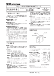
congruent-dissolution approach. The conceptual model used in COMP23 can be represented
by three bodies as shown in Figure 1-1. The bodies are the source, the barrier system, and
the sinks. The source is treated as a well-mixed compartment. The barrier system is the physical medium through which the nuclides migrate to reach the sinks located in the
surrounding system, or outside of the region considered as the barrier system. The sinks,
considered as recipients where the water flows, are fully defined by a local equivalent flow rate.
The purpose of this document is to assist the user in managing problems with COMP23.
An overview of the theory, numerical method, and the code designed to solve the problem
will be presented in the following sections. Finally, an example will be described in detail.
The current version of COMP23 has been extensively revised from earlier versions of
the program. The earlier standalone version of the program was called NUCTRAN.
A description of the earlier version of the program can be found in reference 1.
Sink-1
-
Sink-2
Sink-n
Source
(canister)
(Qeq)
Barrier system
(compartments)
COMP23
Figure 1-1. A schematic of the conceptual model used by COMP23.
FARF31
2
Conceptual model
The presentation of the conceptual model used in COMP23 follows the definition given
by Olsson et al. /2/: “a relatively general description or a definition of the way the model
is constructed. This should be separated from any specific realization or application of the
conceptual model.” The concepts that make up the conceptual model are: specification of
the processes modelled, geometric framework, specification of the parameters, specification
of the assignment of material properties and specification of boundary and initial conditions
required by the model. Each of these concepts will be described for COMP23 in the
following subsections.
2.1
Processes modelled
The processes modelled are radioactive decay and ingrowth, diffusion, advection,
dissolution/precipitation and linear equilibrium sorption. Dissolution and precipitation
are controlled either by a fixed solubility limit for each nuclide or by a solubility limit
shared between nuclides in a solubility group.
The notation used for the equations described in this report is given in Appendix 1.
2.1.1 Radionuclide transport in the barrier
Radionuclides leaking from a damaged canister spread into the backfill material
surrounding the canister and then migrate through different pathways into water-bearing
fractures in the rock surrounding the repository. If the backfill and other materials
surrounding the canister have a low permeability, the solute transport will be only by
diffusion. If there is water flow through some zones of the barrier, then advection may
also be a significant transport mechanism. Some solutes may be sorbed on the materials
surrounding the canister along the transport paths and their migration will be retarded.
Solutes may also precipitate. It is a basic assumption in the COMP23 model that the
dissolution-precipitation reaction is very fast, so that, for nuclides that are solubility limited,
the aqueous concentration will be at the solubility limit if there is any precipitate present.
The COMP23 model allows groups of nuclides to share a solubility limit. For example,
all the isotopes of a given element would be expected to share the same solubility limit.
The nuclides are labelled by consecutive integers, beginning with 1, in such a way that the
parent of nuclide n, if it has one, is always nuclide n-1. Clearly nuclide 1 cannot have a
parent. The fundamental equation expressing material balance for nuclide n is
∂a n
+ u 0 .∇c n − ∇ ⋅ Den ∇c n = −λ n a n + λ n ,.n −1 a n −1 ∂t
(1)
where an is the total amount (dissolved, sorbed and precipitated) of nuclide n per unit
n
volume, cn is the concentration of nuclide n in the pore water, u0 is the Darcy velocity, D e
is the effective diffusivity for nuclide n, λn is the decay constant for nuclide n and λn,n-1 is the
decay constant for nuclide n-1 if nuclide n is the daughter of nuclide n-1 and zero if nuclide
n does not have a parent. Note that the quantities an and cn are functions of both position and
n
time, and that u0 and D e may also depend on position.
Equation (1) is to be regarded as an equation for an, and so cn must be specified as a function
of an. To do this, the assumption that the precipitation/dissolution reaction is very fast is
used. Each nuclide is considered to belong to a solubility group. Normally, there will be
one solubility group for each different element and a group will consist of all the nuclides
that are isotopes of a particular element. Let SE denote the solubility group for element E.
Then SE is the set of labels of the nuclides that are isotopes of element E. The total amount
of element E per unit volume is denoted by aET and it is clear that
a ET =
∑a
m
m∈S E
(2)
The concentration cn, where n ∈SE (i.e. nuclide n is an isotope of element E), may now be
related to an by:
 an

KE
n
c = S n
 cE a
 a ET
if a ET ≤ K E c ES
if a > K E c
T
E
(3)
S
E
where KE is a distribution coefficient for element E and cES is the solubility limit for the
solubility group, SE , of element E. KE is given by
K E = φ E + (1 − φ E )k Ed ρ (4)
where φΕ is the porosity for element E, ρ is the density of the solid material and kEd is
the sorption coefficient for element E. The amount of nuclide n per unit volume that is
in solution is φΕ cn and the amount that is sorbed is (1– φΕ ) kEd ρ, so that the total amount,
dissolved and sorbed, per unit volume is KEcn. Note that the COMP23 model allows the
porosity to depend on the element, so that effects such as anion exclusion can be treated.
Expression (3) may be derived in the following way. When the total amount of element E
per unit volume, aET , is less than the total amount that can be dissolved and sorbed per unit
volume, KE cES , there will be no precipitate of any of the isotopes of E present because of the
assumption that the precipitate dissolution reaction is fast. The amount of nuclide n present
in solution and sorbed per unit volume will be KEcn, and this must be equal to the total
amount of nuclide n present per unit volume so that:
KEcn = an (5)
and the first part of equation (3) follows immediately.
When the total amount of element E per unit volume is greater than the total amount that
can be dissolved and sorbed per unit volume, the aqueous concentration of E will be at the
solubility limit, so that
∑c
m∈S E
m
= c ES (6)
When the system is in equilibrium, the relative proportions of the isotopes must be the same
in the sorbed, dissolved and precipitated material. This means that
(1 − φ E )k Ed ρ c n
(1 − φ E )k Ed c ES
=
φ E c n a n − K E c n =
φ E c ES a ET − K E c ES
(7)
Rearranging equation (7) gives the second part of equation (3). Note that it has been
assumed that all the isotopes of E are chemically identical, so that they have the same
distribution coefficient, KE.
Parameters required
The parameters required are as follow:
• Solid density and porosity of the materials.
• Sorption coefficient and diffusivity of each radionuclide in each of the different materials.
• Solubility limit of each element in each of the different materials.
• Nuclide inventories and half lives.
• The groundwater flux.
2.1.2 Treatment of the source term
In the COMP23 model, the radionuclides in the canister may be present in three forms: in solution in the water in the canister; in the form of precipitate in the canister and embedded in the fuel matrix. It is assumed that there is no sorption in the canister and that the time
taken for the nuclides to mix in the canister is very short, so that the concentration of the
dissolved nuclides is uniform. It is also assumed that the volume of water in the canister is
constant during the calculation. As the fuel matrix dissolves, the actual volume available for
the water in the canister will increase, but since the rate of dissolution is slow, this volume
change can be neglected.
COMP23 treats three types of situation:
I
Solubility limited approach. All species in the canister are available for release,
independently of the structure they are part of. The only limitation in the nuclide
release is the solubility of the individual species.
II A particular case for nuclides initially located at the fuel surface. The handling of this
situation is similar to I but only a fraction of the total nuclide inventory is available
for release.
III Congruent approach for nuclides embedded in a fuel matrix. Since the matrix is
mostly formed by uranium oxide, the release rate for the embedded nuclides depends
on the rate at which the uranium fuel matrix is dissolving. Several models are available
to treat the dissolution of the fuel matrix and the effects of alpha-radiolytically induced
dissolution can be treated. These different models are described in Sections 2.1.4 and 2.1.5.
2.1.3 Source term – solubility limited
The model for cases I and II in Section 2.1.2 is essentially the same. Case I is referred to as
SOL_TYPE OWNSOL and case II as SOL_TYPE FUELSURFACE. Since the dissolved
nuclides in the canister are assumed to be well mixed, the amount of each nuclide in the
canister is determined by a single quantity, ân, that represents the total amount of nuclide
in the canister and that is a function of time. The equation for nuclide n is:
∂aˆ n
= −λ n aˆ n + λ n ,n −1 aˆ n −1 − f n ∂t
(8)
where f n is the rate at which nuclide n leaves the canister by diffusion into the rest of the
barrier system. If σ is the area of the canister that is breached, and so is in direct contact
with the rest of the barrier system, then
f
n
= − ∫ Den n.∇c n (9)
σ
where n is the outward pointing normal to σ, and cn is the concentration of nuclide n in the
barrier system outside the canister, as in the previous section. Again, equation (8) is to be
regarded as an equation for ân. In order to determine f n, and so complete equation (8), the
concentration of nuclide n in the canister, câ n , must be provided as a boundary condition on
σ for the nuclide transport equation outside the canister. The relationship between ân and câ n ,
where nuclide n is an isotope of element E, is
 aˆ n

VC
n
cˆ =  S n
 c E aˆ
 aˆ ET
if aˆ ET ≤ VC c ES
if aˆ > VC c
T
E
(10)
S
E
where VC is the volume occupied by the water in the canister and â ET is the total amount of
element E in the canister:
aˆ ET =
∑ aˆ
m ∈S E
m
The derivation of equation (10) is similar to the derivation of equation (3).
Parameters required
The parameters required are as follow:
• Solubility limit of each element in the water in the canister.
• Volume of water in the canister.
• Nuclide inventories and half lives.
10
(11)
2.1.4 Source term – congruent release without alpha radiolysis
In case III in Section 2.1.2, which is referred to as SOL_TYPE MATRIX, the dissolution of
the uranium fuel matrix, and the consequent liberation of the embedded nuclides, must be
considered. In this case the quantity ân represents the total amount of nuclide n that is in the
canister, but is not embedded in the fuel matrix. In addition, it is necessary to keep track of
the amount of nuclide embedded in the matrix, and this quantity is denoted by bn. Note that
both the ân and bn depend only on time. The equation for nuclide n becomes
∂aˆ n
= −λ n aˆ n + λ n ,n −1 aˆ n −1 − f
∂t
+ qn n
(12)
where qn is the rate at which nuclide n is being liberated from the fuel matrix, which is
given, in terms of the rate at which the uranium matrix is dissolving, by
qn =
bn M
q bM
(13)
where bM is the amount of uranium 238 in the fuel matrix, and qM is the rate of dissolution
of the uranium 238. The basic assumption underlying equation (13) is that the nuclides are
uniformly distributed within the fuel matrix, so that the ratio of the amount of nuclide n to
the amount of matrix is uniform and equal to bn/bM. It is also assumed that all the nuclides
embedded in the matrix are released when the matrix dissolves. Equation (13) follows
immediately from these two assumptions.
The equation for the amount of nuclide n embedded in the matrix, bn, is
∂b n
= −λ n b n + λ n ,n −1b n −1 − q n ∂t
(14)
Equations (12–14) can be used to determine ân and bn only once qM is known. In COMP23,
the way qM is determined depends on whether alpha radiolysis is modelled or not. The case
without alpha radiolysis is considered in this section. The case with alpha radiolysis is
treated in Section 2.1.5.
When alpha radioloysis is not included in the model, the rate of dissolution of the uranium
matrix is determined by the solubility of the uranium in the canister. The model assumes
that the rate at which the matrix dissolves is just fast enough to maintain the uranium in
the water in the canister at its solubility limit without any precipitate forming. A faster rate
of dissolution would obviously lead to the formation of uranium precipitate in the canister
and a situation where the matrix would be dissolving rather than the precipitate, which is
physically unreasonable (in the absence of effects such as alpha radiolysis) and contradicts
the basic assumption that the rate of dissolution of the precipitate is very fast. On the other
hand, it is possible that the matrix could dissolve at a slower rate that is not sufficient to
maintain the dissolved uranium at its solubility limit. However, the current assumption is
conservative and leads to a well defined and relatively simple model.
Summing equation (12) over all the isotopes of uranium and using equation (13) gives
∂
aˆ m = ∑ − λ m a m + λ m ,m −1 aˆ m −1 − f
∑
∂t m ∈SU
m ∈SU
(
m
)+  ∑ b  q
m
M
M  m ∈SU  b
11
(15)
Since the uranium in the water in the canister is at the solubility limit
∑ aˆ
m
m ∈SU
= VC
∑ cˆ
m
m ∈SU
= VC cUS (16)
(17)
)
(18)
so that
∂
∂
aˆ m = VC cUS = 0 ∑
∂t m ∈SU
∂t
Therefore
q =b
M
∑ (λ
M m ∈SU
m
a m − λ m ,m −1 aˆ m −1 + f
∑b
m
m
m ∈SU
To summarize, the model for congruent release of nuclides when there is no alpha radiolysis
consists of equation (12) for each nuclide except nuclide M (the uranium 238 matrix),
equation (14) for all nuclides and equation (16), which effectively determines the amount
of uranium in the canister that is not in the matrix. To complete these equations, qn and qM
are given by equations (13) and (18) respectively.
Parameters required
The parameters required are as follow:
• Solubility limit of each element in the water in the canister.
• Volume of water in the canister.
• Nuclide inventories and half lives.
2.1.5 Source term – congruent release with alpha radiolysis
COMP23 can include the effects of alpha radiolysis on the spent fuel dissolution /3, 4/.
The model assumes that the dissolution rate is related to the alpha-energy release of the
fuel. When an alpha radiolysis model is used an instantaneous release fraction (IRF)
can be specified for each embedded nuclide. This specifies the fraction of the nuclide
that is assumed to dissolve instantaneously. Typically, as the matrix dissolves due to
alpha radiolysis some of the uranium released will form as precipitate and the embedded
nuclides will be freed to dissolve in the water.
Three different representations of the evolving alpha-energy release are included in COMP23.
a) The dissolution rate of the fuel matrix occurs at a constant rate (CONSTANT type).
b) The dissolution rate is a function of the alpha-radiolysis dose rate of the fuel, and
decreases with time as a result of radioactive decay (DECAY type).
c) The dissolution rate is a function of the alpha-radiolysis dose rate of the fuel, and
decreases with time as a result of radioactive decay and dissolution of alpha-emitting
solids from the fuel matrix (EXPLICIT type).
12
The alpha radiolysis model specifies the rate at which the uranium matrix dissolves due to
alpha radiolysis, denoted by qαM . This rate can depend on time and on the amount of various
alpha-emitting nuclides in the matrix, but is independent of the rate at which the uranium is
leaving the canister, which is denoted by qM
.
d
q =b
M
d
∑ (λ
M m ∈SU
m
aˆ m − λ m, m −1 aˆ m + f
∑b
m
)
(19)
(20)
m
m ∈SU
The rate of dissolution of the uranium matrix, qM, is specified by
q M
q M =  dM
qα
if aˆUT ≤ VC cUS
if aˆUT > VC cUS
When the effects of alpha radiolysis are included in the model, the rate of dissolution of the
uranium matrix is always at least the alpha-radiolysis rate. If there is uranium precipitate
in the canister and qαM < qM
the amount of precipitate will decrease until such time as either
d
M
M
qα > qd , or else all the uranium precipitate has been dissolved. The rate of dissolution of
uranium will still be qαM during this period because the precipitate dissolves much more
readily than the matrix. Once all the uranium precipitate in the canister has been dissolved,
it is assumed that the rate of matrix dissolution will be such as to keep the concentration of
uranium in the water at the solubility limit, provided that qαM < qM
still holds. This implies
d
that the rate of dissolution is equal to the rate at which uranium is leaving the canister, qM
.
d
As was pointed out in Section 2.1.4, this particular assumption is conservative. Note that the
uranium concentration in the canister cannot drop below its solubility limit until the entire
uranium matrix has been dissolved (which would take a very long time in most situations).
In previous versions of COMP23 a slightly different model was used in which the uranium
dissolution rate was taken to be the maximum of qαM and qM
. This earlier model would d
imply that in the case where there is uranium precipitate present and qαM < qM
, the matrix
d
would dissolve instead of the precipitate, which is both physically unrealistic and
unnecessarily conservative.
If qαM > qM
, then it is easy to show that there must be uranium precipitate in the canister
d
(see below). So, if there is no precipitate in the canister the maximum of qαM and qM
must be
d
qMd i.e. the first part of equation (20) is equivalent to the original COMP23 model. Thus, the
model represented by equation (20) only differs from the original COMP23 model when
there is uranium precipitate in the canister and qαM < qM
, and then it is physically more
d
realistic than the original COMP23 model, although it is also less conservative.
To prove the assertion made in the previous paragraph, suppose qαM > qM
at time t, then
d
summing equation (12) over all the isotopes of uranium and using equation (13) gives
∂
− λ m aˆ m + λ m ,m −1 aˆ m −1 − f
∑ aˆ m = m∑
∂t m ∈SU
∈SU
(
m
)+  ∑ b  q
m
M
α
M
 m ∈SU  b
13
(21)
Using equation (19) to eliminate the first sum on the right hand side of equation (21) and
rearranging gives
∂
1
aˆ m = M
∑
∂t m ∈SU
b


 ∑ b m qαM − q dM  m ∈S 
 U 
(
)
(22)
m
M
The right hand side of this equation is strictly positive since ∑ b > b > 0 and qαM > qM
d
m ∈SU
by assumption. Thus
∂
∑ aˆ m > 0 ∂t m ∈SU
(23)
which means that the total amount of uranium in the canister that is not embedded in the
fuel matrix is strictly increasing when qαM > qM
. It follows immediately that
d
∑ aˆ
m
(t ) >
m ∈SU
∑ aˆ
m ∈SU
m
(t − δ t ) (24)
for all sufficiently small, positive δt. Since the concentration of uranium in the canister
never drops below its solubility limit until all the fuel matrix has been dissolved
∑ aˆ
m ∈SU
m
(t − δ t ) ≥ VC cUS (25)
(26)
(27)
Combining equations (24) and (25) gives
aUT (t ) =
∑ aˆ
m
(t ) >
m∈SU
∑ aˆ
m∈SU
m
(t − δ t ) ≥ VC cUS as required.
The three models for the alpha-radiolysis dissolution rate, qαM , are:
CONSTANT
qαM = K CON where KCON is a constant.
14
DECAY
4
 t ln 2 
 qαM = K DEC ∑ Ai exp −
i =1
 Bi 
(28)
where KDEC is a constant, t is the time, and Ai,Bi, i = 1,...,4 are constants specific to the
nuclides Am-241, Pu-239, Pu-240 and Np-237 in a particular fuel type /5/. If a different
fuel to that described in reference /5/ is used, the constants will need to be changed in
the program. However, it is not likely that this model will be used extensively as the
CONSTANT model provides an adequate representation of dissolution. The constants,
obtained from reference /5/, are given in the table below.
Nuclide
Ai
Bi
Am-241
25.3
433
Np-237
0.04
2.1·106
Pu-239
1.1
2.4·104
Pu-240
2.2
6,570
EXPLICIT
qαM = K EXP ∑ C m b m m ∈Γ
(29)
where KEXP is a constant, Γ is the set of nuclide labels for the alpha-emitting nuclides,
Cm are constants corresponding to the nuclides in Γ, and bm is the amount of nuclide m in
the fuel matrix. This model is included to allow flexibility of the program. In the current
version of the program the nuclides Am-241, Pu-239, Pu-240 and Np-237 are included and
the values of the constants, obtained from reference /5/, are given in the table below.
Nuclide
C
Am-241
2.85
Np-237
8.81·10–3
Pu-239
0.0261
Pu-240
0.0992
To summarize, the form of the equations representing the model for congruent release of
nuclides including alpha radiolysis depends on whether there is uranium precipitate in the
canister or not. When uranium precipitate is present in the canister the model consists of
equations (12) and (14) for all nuclides together with equations (13) and the second part
of (20). When there is no uranium precipitate present, the model is the same as the case
when there is no alpha radiolysis, described in Section 2.1.4.
15
Parameters required
The parameters required are as follow:
• Solubility limit of each element in the water in the canister.
• Volume of water in the canister.
• Nuclide inventories and half lives.
• Parameters for the alpha-radiolysis dissolution model.
2.2
Geometric framework
To represent the barrier system through which the species are transported, COMP23 makes
use of the integrated finite-difference method /6/ and of the concept of “compartments”.
The barrier system is discretized into compartments. Average properties over these
compartments are associated with nodes within the compartment. From the theoretical
point, of view the compartments may have any shape, but consist of only one material.
The material balance over a compartment is given by:
∂ain
= ∑ g i , j c nj − λ n ain + λ n ,n −1 ain −1 ∂t
j
(30)
where ani is the amount of nuclide n in compartment i, cni is the concentration of nuclide n
in the pore water in compartment i, λn and λn,n–1 are as defined in Section 2.1.1 and gi,j is the
transport coefficient linking compartments i and j. The concentration, cni , where n ∈SE (i.e. nuclide n is an isotope of element E), is related to ani by
 ain
if a ET , i ≤ Vi K E , i c ES

V K
cin =  Si nE , i
T
S
 c E ai
if a E , i > Vi K E , i c E
 a ET , i
(31)
where KE,i is the distribution coefficient for element E in compartment i, Vi is the volume of
compartment i, aET is the total amount of element E in compartment i and cES is the solubility
limit for the solubility group, SE, of element E. KE,i is given by
K E , i = φ E , i + (1 − φ E ,i) k Ed ,i ρ i (32)
d
K
1 − φporosity
where
is(the
for
E, i = φ E, i +
E ,i ) k E ,i ρ
i element E in compartment i, ρi is the density of the solid
material in compartment i and kE,d i is the sorption coefficient for element E in compartment i.
aE,T i is given by
a ET , i =
∑a
m ∈SU
m
i
16
(33)
The diffusional contribution to gi,j is expressed in terms of diffusional resistances.
Each compartment makes a contribution to this resistance. The diffusional resistance
from compartment i to compartment j is Ri,j where
Ri , j =
Ri R j
+
2
2
(34)
and Ri and Rj depend on the direction of transport and the nuclide (through the diffusion
coefficient). Ri takes the form
Ri =
lw
Aw Den,i
(35)
where lw is the length of the compartment in the transport direction (w can be either x, y or z), Aw is the cross-sectional area of the compartment normal to the direction of transport
n
and D e, i is the effective diffusion coefficient for nuclide n in compartment i. Additional
resistances can be added to model special situations, such as transport from a small
compartment into a large one (see the following sections).
The diffusional contribution to gi,j may now be written in terms of Ri,j as
g i, j
 1
if i ≠ j

=  Ri , j
− ∑ g i , j if i = j
 j ≠i
(36)
The elements required to define the compartmentalization are the geometry of the system,
dimensions of the system and the type of material. The compartments are defined by their
volume, their diffusion length and cross-sectional area. Conceptually, the model uses a
rather straightforward compartmentalization process. This coarse compartmentalization
could yield poor or even meaningless numerical results. To avoid this, analytical or semianalytical solutions are introduced in the model in zones where a finite-difference scheme
would require a fine discretization to obtain an accurate result. Some of the approaches
used by the model to describe the solute transport in these sensitive zones are shown below.
2.2.1 Analytical solutions used in the model
The approaches developed at present include transport by diffusion into the flowing water,
transport of solute through a small contacting area into a large volume compartment and
transport of solute into a narrow slit /7/. Other approaches could be included in the code in
the future.
Transport into flowing water
For compartments in contact with water flowing in fractures in the rock, the diffusive
transport is determined by an equivalent flow rate Qeq. This parameter is a fictitious flow
rate of water that carries with it a concentration equal to that at the compartment interface.
17
It has been derived by solving the equations for diffusional transport to the passing water by
boundary layer theory /8/. This entity is obtained from:
Qeq = q o Wη = q o W
4 Dw t w
π
where Dw is the diffusivity in free water, W is the width of the compartment
in contact with
_
water flowing in fractures, fracture zones or damaged zones and η is the mean thickness of
penetration into the water by diffusion from the compartment. The residence time, tw, is the
time that the water is in contact with the compartment. This time is obtained from the flux
of water qo, the flow porosity, and the length of the pathway in contact with water.
Transport into a large compartment
Species diffusing out of a small hole into a very large volume of material spread out
spherically. Very near the hole, the cross-section is still of the order of the size of the hole.
Further away, the cross section increases considerably as the “sphere” grows. Thus, most of
the resistance to diffusion is concentrated very near the mouth of the hole. This resistance is
calculated by integrating the transport rate equation:
N = −2 π r 2 De
dc
dr
from a small hemisphere into a very large volume, between the limits of the sphere of radius
rsph and an outer radius r. Since the species spread over a large volume in the surrounding
medium (r >> rsph), the nuclide transport rate simplifies to N = 2 π rsph De ∆c. In the model,
the real situation is approximated by using an equivalent plug. This plug of a cross-sectional
area equal to the hole area has a thickness Dx given by ∆ x = rhole / 2 .
Transport into a narrow slit
For the diffusive transport into a narrow fracture, most of the resistance to the transport
will be located nearest to the fracture because of the contraction in the cross-sectional area.
The transport resistance is then approximated by a plug through which the nuclides are
transported. The plug has a transport area equal to the cross-sectional area of the fracture,
and a diffusion length equal to a factor times the fracture aperture. Neretnieks analytically
modelled the stationary transport from the bentonite surrounding a canister for spent
nuclear fuel into a fracture /9/. The procedure uses the exact solution of the steady-state
two-dimensional diffusion equation for a sector of the clay barrier representing half the
fracture spacing that allows symmetry conditions to be used. After some simplifications,
the resistance of the plug at the mouth of the fracture is expressed as:
[
]
R f = (Fx , 0 / δ )δ / (De A f ) 18
The factor (Fx,0/d) was calculated by Neretnieks for a number of fracture spacings, fracture
apertures and barrier thicknesses. For fractures with an aperture varying between 10–4 and
10–3 m, and a backfill thickness of 0.30 to 0.35 m, the factor ranges between 3 and 7. It can be visualized as having a plug of clay at the mouth of the slit with a thickness of
(Fx,0/d) times the slit aperture.
2.3
Assignment of material properties
In the standalone version of COMP23, the physical parameters defining the transport in a
repository are specified as constant. In the version to be used as a module in the PROPER
package /10/, the transport parameters, as sorption, diffusion, and equivalent flow rates may
be specified as constant or as functional correlations.
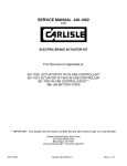
Porosity, sorption coefficient, diffusion coefficient and solubility limit can also be made
time dependent in version 1.2.2 of COMP23. The time dependence can be in the form of
piecewise constant (step) or piecewise-linear (ramp) variations. These are illustrated in
the figure below.
Parameter
Piecewise linear
T1
T2
T3
time
Parameter
Piecewise constant
T1
T2
T3
19
time
2.4
Initial conditions
COMP23 solves an initial value problem, comprising a system of differential and possibly
algebraic equations. The solution of this system is straightforward once the initial conditions
have been defined. The variables defining these conditions are determined by the amount of
the species dissolved, the amount of the species as solid inventory in the compartments and
the amounts of nuclides embedded in the fuel matrix when a congruent dissolution model is
used. The default initial condition is zero for all compartments, except for the compartment
acting as the source where the initial condition is determined by the inventory and the
solubility of the species.
20
3
Numerical methods
3.1
Spatial discretization
The compartment model COMP23 formulates the near-field transport in terms of integrated
finite differences, introducing the concept of “compartments” to define the discretization
of the system. This concept is very useful when the transport is through materials with different properties and the geometry of the whole system is complex. The compartment is
fully defined by its capacity and the resistances defining a two-dimensional nuclide transport.
The capacity is determined by the volume and the sorption coefficient, and will also depend
on the porosity and density of the material. The diffusion length(s), cross sectional area(s),
and the diffusion coefficient define the resistance. The compartmentalization of the system
is rather straightforward. The system to be modelled is subdivided into compartments taking
into consideration the different geometric shapes and the various materials found in the
system. COMP23 uses a coarse discretization.
3.2
Temporal discretization
Once the spatial discretisation has been carried out, the equations to be solved consist of a
set of ordinary differential equations for the amounts of each nuclide in each compartment,
ani , in the form of equation (30). In the congruent dissolution model, equation (14) for the
amount of each nuclide in the matrix, bn, must also be solved, together with the algebraic
equation (19) for the rate at which uranium is leaving the canister. These equations may be
written in the general form
F ( y& , y, t ) = 0 (37)
where y is a vector comprising all the ani (and bn and qM
when congruent dissolution is being
d
&
F ( y,isy,the
t ) =time
0 derivative of y. These equations are stiff, due to the wide range
treated), and
of timescales in the problem. COMP23 uses the package DDASKR to solve this system of
implicit differential-algebraic equations (DAES). The package uses backward difference
methods of varying order of accuracy1, and chooses the order and the size of the time-step
to maintain a specified level of accuracy whilst minimizing the computational time /11/.
DDASKR can produce results at intermediate time very efficiently. The user of COMP23
specifies points at which output is needed. DDASKR also has a facility for monitoring user
defined functions and finding the time at which any of these functions becomes zero.
The methods used in DDASKR rely on the solution to the equations (37) being sufficiently
smooth. The degree of smoothness required depends on the highest order of method to
be used, which is typically 5. The main technical difficulty with the equations arising in
COMP23 is that the smoothness assumption breaks down at various points in time, such as
when the amount of nuclide in a compartment exceeds the solubility limit, or when the size
of the hole in the canister changes abruptly, or when the rate of uranium dissolution changes
type in the congruent release model. This is dealt with in COMP23 by monitoring various
1
A method of order n has an error that is proportional to the nth power of the size of the timestep.
21
quantities that mark these changes. The root finding capabilities in DDASKR are used to
identify the precise time at which the change takes place. The computation is then restarted
from that time using the appropriate new set of equations. The essential point here is that
DDASKR is only ever solving smooth systems of equations, and so its methods work well
and the program is reasonably robust.
The conditions that are monitored by the code will now be described. When the OWNSOL
or FUELSURFACE models are used the following quantities are monitored:
• ∑a
m ∈S E
m
i
− Vi K E , i c ES for each compartment i and each element E. When this quantity
passes through zero and is increasing, the element E is changing from being not
solubility limited to being solubility limited (and the other way round if the quantity
is decreasing). When the quantity changes sign, the calculation is restarted using the
appropriate form of equation (31) to compute cni in terms of ani .
• Times at which the size of the hole in the canister changes abruptly. In these cases some
of the coefficients in the equations change. When COMP23 detects an abrupt change
in the hole size, it recalculates the relevant coefficients and restarts the calculation.
When the MATRIX model is used the following quantities are monitored:
• ∑a
m ∈S E
m
i
− Vi K E , i c ES for each compartment i, and each element E except for uranium in
the canister. When this quantity passes through zero and is increasing, the element E is
changing from being not solubility limited to being solubility limited (and the other way
round if the quantity is decreasing). When the quantity changes sign, the calculation is
restarted using the appropriate form of equation (31) to compute cni in terms of ani .
• bM – the amount of uranium 238 in the fuel matrix. When this quantity becomes zero
the calculation is restarted without fuel dissolution. The model becomes the same as the
OWNSOL or FUELSURFACE models.
• Times at which the size of the hole in the canister changes abruptly. In this cases some of
the coefficients in the equations change. When COMP23 detects an abrupt change in the
hole size, it recalculates the relevant coefficients and restarts the calculation.
The other quantity to be monitored depends on whether uranium precipitate is present in the
canister or not. If uranium precipitate is present, then the following quantity is monitored:
• ∑a
m ∈SU
m
1
− VC cUS where by convention, compartment 1 is the canister. This quantity should only pass through zero in the decreasing direction (otherwise there cannot be
uranium precipitate in the canister). When this quantity passes through zero, the rate
of dissolution due to alpha radiolysis is not sufficiently high to keep the uranium in the
canister at the solubility limit, so the fuel matrix dissolution rate will be controlled by
rate at which uranium is leaving the canister. The calculation is restarted with the amount
of uranium 238 in the canister that is not in the matrix being calculated from equation (16).
22
If there is no uranium precipitate present in the canister, then the following quantity is monitored:
• qα − q d . Initially, this quantity must be negative (otherwise there would be uranium
precipitate present – see the discussion in Section 2.1.5). When this quantity goes through
zero uranium is about to be precipitated in the canister. The calculation is restarted using
qαM as the fuel matrix dissolution rate and solving equations for all the nuclide amounts,
including the uranium 238. It can be shown that when the calculation is restarted, the
rate of increase of uranium precipitate in the canister is initially zero, but that the second
derivative of the total amount of uranium in the canister is positive. So, although uranium
will be precipitated, the initial amount precipitated will be small. This can cause numerical
problems if the accuracy of the solution is not sufficiently high.
M
M
Finally, note that the case when there is no alpha radiolysis can be considered as a special
instance of the case with alpha radiolysis with qαM = 0 as far as the quantities monitored
is concerned.
23
4
Description of the COMP23 code
The COMP23 code is written in FORTRAN. There are two versions depending on the
environment it works in: a standalone version and a special version to be used as a
submodel of the PROPER code. The code consists mainly of three parts that are:
MAIN PROGRAM:
SOLVER:
INPUT FILES:
CMP23
DDASKR
system.dsc, casename.inv, casename.nam and submod.lib
The main program CMP23 makes use of several subroutines that will be described later.
The INPUT files are described in detail in the next sections.
The code solves three types of specific situations:
I
Solubility limited approach. All species in the canister are available for release,
independently of the structure they are part of. The only limitation on the nuclide
release is the solubility of the individual species.
II A particular case for nuclides initially located at the fuel surface. The handling of this
situation is similar to I but considers that only a fraction of the total nuclide inventory
is available for release.
III Congruent approach for nuclides embedded in a fuel matrix. Since the matrix is mostly
formed by uranium oxide, the escape rate for the embedded nuclides will depend on the
escape rate of the uranium. Thus, to calculate the release of these nuclides, the U-238 is
simultaneously run with the nuclides of interest.
The solubility limits may be either fixed or calculated from a shared solubility limit for a
group of nuclides.
There are also special uses of the code that are easy to manage. They are:
a) Addition of a transport resistance between two compartments. The code needs know
only the value and where the resistance will be placed.
b) The damage in the canister wall is handled as a special compartment where the user has
the alternative of choosing a growing hole or a hole of stationary size. For the situation
of a growing hole, the user may choose a linear function or a step function for the growth.
c) Addition of a plug at the outlet of the source in order to approximate the mass transport
between a small compartment and a large one. This is applied to the nuclide transport
from the small hole in the canister wall into the bentonite outside the hole.
d) Addition of a plug situated inside the canister (source) when the backfill material is
granulated. This is a special use for copper/iron canister as source, where the nuclide
transport into the damage in the canister wall is approximated by a plug at the inlet of
the damage. This plug has the same dimensions as the plug at the outlet of the damage.
The effective diffusion coefficient (De) is established beforehand and is 10–10 m2/s.
Note:
The dimensions of both plugs (inlet and outlet) depend on the size of the hole at the canister
wall. So if the size of the hole varies, the dimensions of both plugs vary too.
25
4.1
Subroutines and functions used by COMP23
4.1.1 Key variables used by the subroutines
AREA:
variable that defines the cross-sectional area for a compartment whose size
changes with time.
AGQ:
partial matrix of constant coefficients.
AINV:
vector storing the input amount (inventory) of the species.
EPS:
requested relative accuracy in all solution components.
EWT:
problem zero, i.e. the smallest physically meaningful value for the solution.
ICALL:
index controlling the recall of the solver from the main program or the
stopping of the program execution.
ICH:
index identifying the decay chain number.
INABS
absolute index identifying a nuclide without reference to a chain.
INUC:
index identifying the nuclide in a chain.
IPRINT:
position index in the time series.
ISPSOL:
shared solubility flag: = 0 if no shared solubility, = 1 if shared solubility
is required.
NEQ:
the number of differential equations.
NROOT:
the number of equations whose roots are desired. If NROOT is zero, the root
search is not active. This option is useful for obtaining output at points that are not known in advance, but depend upon the solution.
QDURAN: dissolution rate of the fuel matrix.
ADURAN: dissolution rate of the fuel matrix due to alpha radiolysis.
T:
independent variable in the ODEs/DAEs.
TIME:
independent variable in the ODEs/DAEs.
TOUT:
the point (time) at which the solution is desired.
Y:
vector of nuclide amounts – solution of ODEs/DAEs.
YPRIME:
vector of derivatives of the solution to the ODEs /DAEs.
4.1.2 Description of key subroutines
ALPH23 ( TIME, Y, ADURAN )
This subroutine calculates the dissolution rate of the fuel matrix (U238), ADURAN, due to
alpha radiolysis.
CONC23 ( Y, IPRINT, ICALL )
This subroutine stores the output data, such as concentrations for all compartments and time
at which they were calculated. The main program CMP23 calls CONC23.
CSTO23 ( IPRINT, ICALL, T, Y )
This subroutine called by CMP23 if DDASKR indicates that a zero has been found in one
of the conditions being monitored. It sets LSOLIM and IMFLAG do indicate the change
in the equations to be solved. It also sets the flag ICALL to indicate whether initialisation
needs to be carried out or if a fatal error has occurred.
26
DDASKR ( SSRES, NEQ, T, Y, YPRIME, TOUT, INFO, RTOL, ATOL, IDID, RWORK,
LRW, IWORK, LIW, RPAR, IPAR, SSJAC, PSOL, SSRT, MROOT, JRTSS )
This subroutine solves the implicit differential-algebraic equations (DAEs) of the form
F ( y& , y, t ) = 0 , given the initial conditions y0 = y(t = 0) which must be used to supply
F ( y&0,.yDDASKR
, t ) = 0 is called once for each output point of T.
consistent initial values for
The subroutines SSRES, SSJAC and SSRT are part of COMP23 and their functions are
described below. The main program CMP23 calls DDASRT.
FLOW23 ( IFSTOP, IPRINT, MULTI )
This subroutine calculates the release, by molar flow rate, from the source and into the
various sinks. These data are written to the PROPER database via a call to PUTS. The time
series at which the molar flow rates are calculated is determined beforehand by the user.
The main program CMP23 calls FLOW23.
FMCO23 ( ICH )
This subroutine defines the coupling resistances between compartments, including the
external coupling with the flowing water surrounding the barrier system. FMCO23 is
called by IMAT23.
FMDE23 ( ICH )
This subroutine defines the capacity and individual resistances to transport of all
compartments. FMDE23 is called by IMAT23.
MAT23 ( TIME )
This subroutine computes the coefficients that appear the governing equations. MAT23 is
called by IMAT23.
PRIN23 ( IPRINT, NAMES )
This subroutine prints out results of the execution such as concentrations in the various
compartments, release into the various sinks and solid inventory in the canister. The results
are printed at times determined by TIME23. It also prints out the variation with time of the
hole size in the canister wall. The main program CMP23 calls PRIN23.
READ23 ( NAMES, EPS, EWT, NLOOP, NPREPAR, LSTALON, U0, CASE )
This subroutine reads the data from the INPUT files with help of an auxiliary subroutine
HUIM23 created specially to operate in the PROPER environment. The main program
CMP23 calls READ23.
SET23 ( NAMES, Y, CASE )
This subroutine sets the initial conditions for the problem and the flags (IFLAG) for
the material balance control in the various compartments. The main program CMP23
calls SET23.
SSJAC ( NEQ, TIME, Y, YPRIME, PD, CJ, RPAR, IPAR )
This subroutine computes the Jacobian matrix for F ( y& , y, t ), =the
0 equations defining the
DAE at time, to be evaluated at Y, YRPIME and TIME. A return from this function passes
control back to DDASKR.
27
SSRES ( TIME, Y, YPRIME, CJ, DELTA, IRES, RPAR, IPAR )
This subroutine computes F ( y& , y, t ), =the
0 equations defining the DAEs. When this subroutine
is called, the entries in Y are intermediate approximations to the solution components and
the entries in YPRIME are intermediate approximations to their derivatives. A return from
this function passes control back to DDASKR.
SSRT ( NEQ, TIME, Y, YPRIME, NRT, RVAL, RPAR, IPAR )
This subroutine computes the values of the various functions being monitored by
DDASKR. A return from this function passes control back to DDASKR.
SSINI ( TIME, Y, YPRIME )
y, t ) = 0 based on the values of y (Y) at time t (TIME).
Calculates the values F
of( y& ,(YPRIME)
TIME23 ( TINIT, ICALL )
This subroutine determines the time series at which the user wishes to obtain results.
The time step is determined by a geometric progression. The main program CMP23
calls TIME23.
URC23 ( TIME )
This subroutine updates the coupling resistances between compartments, including
the external coupling with the flowing water surrounding the barrier system to taking
into account the effect changes in the size of the hole in the canister. URC23 is called
by IMAT23.
WRIT23 ( NAMES )
This subroutine gives information on capacities and resistances of the various
compartments. It also gives information on the matrix of the coefficients “F” initially
executed. WRIT23 is called by FMAT23.
4.1.3 Additional subroutines
A description of these subroutines is found in the Proper Monitor User’s Manual /12/ and
Proper Submodel Designer’s Manual /10/. These subroutines are implemented and of use
only in the PROPER version of the code COMP23. Some of them are part of the PROPER
package. “They are service routines for setting up communications with the database, for
acquiring values of sampled parameters, for handling time series and for handling data from
external submodel-specific files” /10/.
INVEN ( FILNAM, IUNAM, FILINV, IUINV, NNUCL, NAMES, TBREAK, AINV )
This subroutine gives information on the inventory in the canister. SET23 calls INVEN.
PRELUD ( FILE )
Set up communication with the internal database.
POSLUD
Closing down communication with the internal database.
GETP ( INDEX )
Used to obtain sampled parameters from the internal database.
28
PUTS ( IDD, TSERIE, VALUE )
Used to send output time series to the internal database.
To avoid conflict, service routines are used to obtain an unused unit number and the
unique name of a data file when opening. They are:
IGETUN ( IDUM )
GETDAT ( IDUM )
to get the unit number.
to get the unique name of a data file.
and when closing the file
PUTUN ( IUDAT ) 4.2
to return the unit number to the monitor.
General description of the input requrements
The physical geometry of the system is simplified by dividing it into blocks. The blocks are
numbered in ascending order. The discretization in blocks considers the geometry and the
various materials by which the nuclides migrate. Not all blocks have the same geometry and
orientation, so each block has its own axes of references. So far there are only two transport
directions defined for the block (horizontal (x or y) direction and z-direction).
The transport in a block is completely defined by the physical properties of the material, the
nuclide transport properties and the geometrical dimensions of the block. These properties
are used by the code to calculate the capacity of the block and its resistance to transport for
each of the two defined transport directions. These data are the input data for the problem to
be solved. The capacity and the resistance are determined by the following expressions:
Capacity = V [φ + (1− φ)k d ρ ]
Resistance =
x
ADe
where x is the diffusion length of the block (in the direction of transport), A is the cross-
sectional area of the block (perpendicular to the direction of transport) and De is the
effective diffusion coefficient. The porosity and the density of the material solid are denoted
kd is the sorption coefficient and V is the volume of the block.
φ E )k Ed ρ
K Eby= φ Eand
+ (1ρ−respectively,
As two transport directions have been defined, the code needs to know the geometrical
dimensions of the block for both directions to define the transport. Such geometrical
dimensions are diffusion length and cross-sectional area for each direction. The volume
of the block is calculated by the code from the given dimensions for transport in the
z-direction.
Any block, except the source, may be subdivided into compartments in any of the two
directions named above. The block itself is a compartment if it is not subdivided. A simple
subdivision is that by discretization in the z-direction the code makes the block into
compartments of equal capacities. The code needs only to know the desired number of
subdivisions in the z-direction NZ, so that NX = NY = 1, which means no subdivision in
the x or y directions. For any other subdivision, all compartments have to be defined in the
INPUT file. The compartments are numbered by the code following the z-axis for the block,
while the other direction is kept constant.
29
The first block defined in the INPUT data is the source (interior of the canister) followed by
the block describing the damage of the source (hole in the canister wall).
Each block may be connected to one or more than one block, except the source. At present,
the source can only be connected to one compartment. Each couple of connected blocks (A and B) is specified by the user in the INPUT file. Several control numbers define the
connection. Such numbers are used to define: the position of each block (A and B), the
numbers of the couples of compartments involved in the connection of block A and B, the
direction (z-axis or x or y-axis) of each block and the contribution of each block to the
coupling resistance. After the connection of the two blocks is specified, the code needs to
know the position of the couples of compartments involved in each connection. All this
information is used to calculate the coupling resistance Ri,j:
Ri , j =
Ri R j
+ 2
2
where Ri and Rj are the individual resistances of the compartment “i” and the adjacent
compartment “j” respectively.
External resistances specified in the input data may be added between two blocks.
For resistances added in the form of a plug, these are codified by IPLUG = index (block
number A or B). This index block is used by the code to obtain the diffusion coefficient.
This plug concept is very useful when the transport is between a block of very small volume (block A) and a block of large volume (block B). The plug resistance value is:
plug resistance =
Ahole / (2 π )
De Ahole
=
1
De 2π Ahole
where Ahole is the cross-sectional area of the block of small capacity. Suppose that for some
A-B connection, IPLUG = block B number (block of large capacity). Then, the coupling
resistance calculated by the code is:
Coupling resistance Rab =
Ra
+ plug resistance
2
The size of the block of small capacity may vary with time. If this is the case, the plug
resistance will also vary. The existence of other types of resistances added to the connection
are indicated by IRADD = 1, whose values are given following the description for such
effects in the input file. Suppose that for some A-B connection, IRADD = 1. If the user
specifies the resistance value as RADD, the calculated coupling resistance is:
Coupling resistance Rab =
Ra
R
+ RADD + b
2
2
30
The connections of the various sinks to the system (repository) are defined by identifying
the position of the block and compartment connected to each sink. In addition, the user
has to codify the direction of the nuclide transport (IRZ) and the contribution of the
compartment to the coupling resistance (ICRS). For the situation of one fracture intersecting the system, a plug approximates the nuclide transport into the fracture.
The dimension of this plug have to be defined by the user. For this situation ICRS = 0.
As the code for COMP23 exists in two different operative versions, there are two input
data files. The differences between them are in the structure of the subroutines to read
the input data, to process the output data, and to get information of the initial nuclide
inventory. The variable definition is the same for both versions. In the standalone version
of COMP23, the nuclide inventory has to be given in the INPUT file. In the PROPER
version of COMP23, the nuclide inventory is implicitly obtained by the code; it needs only
to know the names of the nuclides and the break-time (TINIT) for the canister. In the next
section, the INPUT file for the PROPER version will be presented. The standalone version
is described in a separate manual.
31
5
Simulation setup using Proper
5.1
Overview
COMP23 can be run as a submodel of the PROPER package. A User Guide for the
PROPER package is given in reference /12/. This section gives details specific to
running COMP23 as a submodel of PROPER.
Section 5.2 describes the input files that are required by the PROPER package when
COMP23 is included as a submodel.
The PROPER version of COMP23 uses the HYDRASTAR User Interface (HUI) /13/.
HUI is a preprocessing facility incorporated into the HYDRASTAR code and the
COMP23 code. The main objectives of the HUI are:
• Free-format input in a single input file.
• Input data validity testing.
• Input data consistency checking.
A general description of the HUI input file is given in Section 5.3 of this report. A detailed description of the COMP23 input required is given in Section 5.4.
Details of the output produced by the HUI interface are discussed in Section 5.5.
5.2
Input files required
The following input files are required to run COMP23 as a submodel of PROPER:
Name
Description
system.dsc
The system description file that is used for all PROPER simulations. The input requirements
for this file are described in more detail below.
casename.inv,
casename.nam
These two files hold the information on the radionuclide inventories for one canister. The inventory files used by COMP23 are identical to the files used by TULLGARN /14/,
so these two files should preferably be links if TULLGARN is used in the same simulation.
casename is read in from the CONTROL block of the system.dsc file.
submod.lib
Lists the modules that are used by PROPER. The module name for COMP23 is COMP23
and it is connected as an internal submodel /12/.
5.3
HUI input
The following notational conventions are used to describe the format of the input data for this
model. In general the definition follows that of INFERENS /15/. A detailed description of
the input required when running the PROPER version of COMP23 is given in Section 5.4.
33
5.3.1 Typefaces
CAPITAL
lowercase italics
CAPITAL ITALICS
underlined
bold underline
Keywords
Variable name or variable text.
Object name or name of variable in the code.
Fixed text.
Program validity check.
5.3.2 Separators
# {}
[] | @
+ <>
Beginning of comment.
List of items.
Enclosed list of optional items.
Optional items separator.
Zero or more occurrences of preceding expression.
One or more occurrences of preceding expression.
Keystrokes or special characters.
5.3.3 Format specifiers
A*
A*:wordlist
F*
I* wordlist
Free-format string.
Free-format string; must be member of wordlist.
Free-format floating point number.
Free-format integer.
List of alternative keywords [word1|...|wordN] which are allowed for the specified context.
5.3.4 Program validity check
V C E W
Validity
Consistency
Existence
Warning
5.3.5 Format syntax
{input_file} =
[system_commands]@
[{a_block} | {comments} ]+
{a_block} =
BEGIN_BLOCK block_id
{block_definition}
END_BLOCK
{block_definition} =
[{keywords} |
{lists}|
{definition_block} |
{switchcommands} |
{comments} ]+
{keywords} =
KEYWORD [I*|F*|A*|A*:wordlist| ]+ [{comments}]
34
{lists} =
KEYWORD
[I*|F*|A*|A*:wordlist| ]+ [{comments}]
END_LIST
{definition_block} =
BEGIN_DEF def_id
[ [{keywords} | {comments} ]+ | [I*|F*|A*|A*:wordlist| ]+ ]
END_DEF
{switch_command} =
switch (switch_var)
case VALUE1:
{keywords}
...
case VALUEn:
{keywords}
endswitch
{comments} =
’ #’ {any_text} {end_of_line}
system_commands =
SYSTEM KEYWORD
5.4
The system description file
5.4.1 Overview
The system description file, system.dsc, is used to specify for PROPER the module
intercommunication, sampled parameters etc. The general format of the system description
file is (only the parts relevant to this manual have been included):
PROPER_KEYWORDS
MACROS definitions
PARAMETERS section
MODULE definitions
each MODULE definition has the general format:
MODULE module (Input_Timeseries; Output_Timeseries)
INPAR section
DATA section
END module
Note: the order of the INPAR and DATA sections is not significant.
Any lines beginning with the ’#’-character are handled as a comment line.
35
5.4.2 Parameters
The PARAMETERS section in the system description file defines the sampled parameters
and their distributions. The general syntax for the PARAMETERS section is:
PARAMETERS
Parameter_name distribution_type [(arg1[,arg2[...]] )]
END PARAMETERS
The order in which the parameters are passed to COMP23 is defined within the INPAR
section within the MODULE definition. The general syntax for the INPAR section is:
INPAR
parameter_name1 [parameter_name2 ...]
END INPAR
No Time-dependent Parameters
The following parameters need to be defined in the PARAMETERS section for COMP23. A detailed description of the parameters is given below.
Suggested name(s)
Description
CSYNC
Random number seed.
MULT
The number of canisters the calculation segment (normally from
HYDRASTAR).
PROB
Probability for initial damage to canister.
PITFAQ, QS, CONHS, DEFFS
Corrosion data (not used by present version of the model ).
DENS
Density of different barrier materials (if not defined in BLOCK data).
POR
Porosity of different barrier materials (if not defined in BLOCK data).
T_HOLE, A_HOLE
Hole growth data for chosen growth model.
CSOL
Solubility of the nuclides.
DIF
Effective diffusion coefficient in the different barrier materials for all nuclides.
KD
Kd-value in the different barrier materials for all nuclides.
VTUBE, NTUBES, NTDAM,
VHEMA
Tube volume, number of tubes, tubes damaged and void (if not defined in
BLOCK data).
AER
Alpha-radiolysis parameter K for chosen model (if required).
ZRFRA, APFRA, QFAC, QEXP
Data for each sink (if not defined in BLOCK data).
IRF
Instantaneous Release Fraction (IRF) values (only required for nuclides that
use a FUELSURFACE or alpha-radiolysis model).
The order that these are listed above is the order that the parameters must be specified
within the INPAR section. When COMP23 is used as a standalone model two extra
parameters are given as the first parameters. These are NCAN and UC.
Suggested name
Units
Description
NCAN
(–)
Number of canisters to be modelled (recommended value 1). (Only used for standalone version)
UC
(m3/m2/yr) Water flow rate outside canister. (Only used for standalone version)
CSYNC
(–)
Random number seed.
MULT
(–)
Number of (assumed identical) canisters in region.
PROB
(–)
Probability of a single canister being penetrated at time of emplacement.
36
If COMP23 finds that there is a single canister that has been penetrated at time of
emplacement, it ignores the other canisters and calculates the rate using one initially
damaged canister. If no canister is initially damaged, no release calculations are performed
in the present version.
The next parameters define the densities of the barrier materials. They must be present if
this data is not defined in the MATERIAL section of the GEOMETRY block but will be
overridden by that data if it is present.
Suggested name
Units
Description
DENS m
(kg/m )
Density of barrier material m.
3
The next parameters define the porosities of the barrier materials. They must be present
if this data is not defined in the MATERIAL section of the GEOMETRY block but will
be overridden by that data if it is present. If the System Command USE_NUCLIDE_
DEPENDENT_POROSITIES is present, then the porosity data must be entered here and
must not be entered in the MATERIAL section of the GEOMETRY block. In this case the
porosity for each nuclide, in each material must be entered.
If the System Command USE_NUCLIDE_DEPENDENT_POROSITIES is not present:
Suggested name
Units
Description
POR m
(–)
Porosity of barrier material m.
If the System Command USE_NUCLIDE_DEPENDENT_POROSITIES is present:
Suggested name
Units
Description
POR nm
(–)
Porosity of barrier for nuclide n
in material m.
The next group of parameters defines the hole growth depending on the hole growth model
chosen. For each step in the hole growth model a time and area must be given including the
initial and final times.
Suggested name
Units
Description
T_HOLE n
(y)
Time at which following are is
attained.
A_HOLE n
(m2)
Area of hole.
For example if the hole growth model is a linear ramp from the initial size to the final size
the following data would be given:
T_HOLE0 CONST (1.0E+3)
A_HOLE0 CONST(1.0E–6)
T_HOLE1 CONST(1.0E+6)
A_HOLE1 CONST(2.0E–3)
The next parameter defines the solubility of the nuclides:. If the system command USE_
MATERIAL_DEPENDENT_SOLUBILITY_LIMITS is not present:
Suggested name
Units
Description
CSOL
(mol/m )
3
Solubility for the nuclides, one
parameter for each nuclide n.
37
For example, if two nuclides (A and B) are used the definition would look like:
CSOLA CONST (2.0E–4)
CSOLB CONST (2.0E–5)
If the system command USE_MATERIAL_DEPENDENT_SOLUBILITY_LIMITS is
present, then a solubility limit is required for each material. For example, if two materials,
M1 and M2 are present, then the definition would look like:
CSOLAM1 CONST (2.0E–4)
CSOLBM1 CONST (2.0E–5)
CSOLAM2 CONST (2.0E–3)
CSOLBM2 CONST (2.0E–3)
The next parameters are repeated in the order stated below, for each material type in the
model. Usually there are four materials used, water, bentonite, sand-bentonite and rock.
For every material type, the data for every nuclide must be defined. Note that the order of
nuclides as defined within the DATA section must be followed.
Suggested name
Units
Description
DIF nm
(m2/year)
Effective diffusivity for nuclide n
in material m.
KD nm
(m3/kg)
Kd for nuclide n in material m.
For example, if two nuclides (A and B) and four materials (1 to 4) are used the definition
would look like:
# Specific to material 1
DIFA1 CONST (0.123E0)
DIFB1 CONST (0.123E0)
KDA1 CONST (0.0E0)
KDB1 CONST (0.0E0)
#
# Specific to material 2
DIFA2 CONST (0.3154E–2)
DIFB2 CONST (0.3154E–2)
KDA2 CONST (3.0E0)
KDB2 CONST (3.0E0)
#
# Specific to material 3
DIFA3 CONST (0.3154E–2)
DIFB3 CONST (0.3154E–2)
KDA3 CONST (0.1E0)
KDB3 CONST (0.1E0)
#
# Specific to material 4
DIFA4 CONST (3.1536E–6)
DIFB4 CONST (3.1536E–6)
KDA4 CONST (3.0E0)
KDB4 CONST (3.0E0)
38
Time-dependent Parameters
When it is necessary to incorporate time-dependent parameters into a system model, extra
parameters must be specified that define the times at which ramp or step changes occur
(see Section 2.3), and also the values of the various parameters in each of the different time
regimes. Sorption coefficient, porosity, diffusion coefficient and solubility limit can all be
made time dependent.
In order to explain the procedure for setting up time-dependent parameters in COMP23, it
is easier to proceed with an example. Suppose, in the examples given above, it is desired to
make the diffusion coefficient for nuclide A in material 1 piecewise-constant as shown in
the figure in Section 2.3. It is first necessary to define the times T1, T2 and T3 in system.
dsc. For example, this could be done as follows:
TIME_T1 CONST(1.0E2)
TIME_T2 CONST(1.0E4)
TIME_T3 CONST(1.0E5)
Next, it is necessary to define the values of the diffusion coefficient for the various time
regimes. For example:
DIFA1T1 CONST (0.123E–2)
DIFA1T2 CONST (0.123E–1)
DIFA1T3 CONST (0.123E0)
For the non-time-dependent case described in the previous subsection, the INPAR section
would contain the following lines in the appropriate place:
DIFA1 DIFB1 DIFA2 DIFB2 DIFA3 DIFB3 DIFA4 DIFB4 KDA1
KDB1
KDA2
KDB2
KDA3
KDB3
KDA4
KDB4
In the time-dependent example we are considering, the INPAR section would look
as follows:
TIME_T1
DIFA1T1
DIFB1 DIFA2 DIFB2 DIFA3 DIFB3 DIFA4 DIFB4 KDA1
KDB1
KDA2
KDB2
KDA3
KDB3
KDA4
KDB4
39
TIME_T2
DIFA1T2
DIFB1 DIFA2 DIFB2 DIFA3 DIFB3 DIFA4 DIFB4 KDA1
KDB1
KDA2
KDB2
KDA3
KDB3
KDA4
KDB4
TIME_T3
DIFA1T3
DIFB1 DIFA2 DIFB2 DIFA3 DIFB3 DIFA4 DIFB4 KDA1
KDB1
KDA2
KDB2
KDA3
KDB3
KDA4
KDB4
It should be noted that it is necessary to define all of the parameters for all of the time
regimes. In words, this INPAR section states that for times between 0 and T1, the diffusion
coefficient takes a value DIFA1T1. Between times T1 and T2, it takes the value DIFA1T2.
Between times T2 and T3 it takes the value DIFA1T3.
Time dependence for the porosity and solubility limits are set up in a very similar way, and
the corresponding parts of the INPAR section of system.dsc must be written in the form
shown above.
It is also necessary to specify, in the control block, the details of the form of the time
dependence that is to be modelled (see Section 5.4.4, subtitle Control block definition).
Remaining Parameters
The next parameters give details of the modelled canister comprising a number of tubes
surrounded by void space. The number of damaged tubes is specified here. They must be
present if this data is not defined in the GEOMETRY block but will be overridden by that
data if it is present.
Suggested name
Units
Description
VTUBE
(m )
Volume of water in one tube in the canister.
NTUBES
(–)
Total number of tubes in the canister.
NTDAM
(–)
Number of damaged tubes in the canister.
VOID
(m )
Water volume inside the canister.
3
3
40
The next parameter is the constant in the alpha-radiolysis model. It’s exact meaning and
units will depend on the model chosen, see Section 2.1.5. It is optional but must be present
if alpha-radiolysis is modelled.
Suggested name
Units
Description
AER
(depends on model)
Alpha-radiolysis parameter K for chosen
model (if required).
The next parameters define the sink data and must be present if this data is not defined
in the SINK section of the GEOMETRY block but will be overridden by that data if it
is present.
Suggested name
Units
Description
PLUG_LEN n
(m)
Length of the plug (extra resistance) added
to the connection between compartment and
sink n.
PLUG_AREA n
(m2)
Cross-sectional area of the plug added to the
connection between compartment and sink n.
This parameter must be positive.
QFAC n
(–)
See below.
QEXP n
(–)
See below.
The QFAC and QEXP values are used to calculate the equivalent groundwater flow at the
sink according to the formula:
Qeq = QFAC. qQEXP
where q is the groundwater flux at the canister position obtained from HYDRASTAR.
For example, if two sinks are used the definition would be as follows:
# Sink 1
PLUG_LEN1 PLUG_AREA1
QFAC1
EQXP1
#
# Sink 2
PLUG_LEN2 PLUG_AREA2
QFAC2
EQXP2
CONST (5.0E–4)
CONST (5.5E–4)
CONST (0.03)
CONST (0.5)
CONST (0.002)
CONST (0.006)
CONST (1.0)
CONST (0.5)
The next parameter defines the IRF for the nuclides in the model. Note that the order of
nuclides as defined within the DATA section must be followed.
Suggested name
Units
Description
IRF n
(–)
Instantaneous Release Fraction for nuclide
n. One value for each nuclide that uses a
FUELSURFACE or alpha-radiolysis model.
41
For example, if two nuclides (A and B) are used the definition would look like:
# IRF values (only for FUELSURFACE or alpha-radiolysis models)
IRFA CONST (0.1E0)
IRFB CONST (0.1E0)
5.4.3 Input timeseries
As with the TULLGARN code, COMP23 needs to obtain the Darcy groundwater velocities
outside the canister(s) as an input timeseries from another model.
There are three pseudo-timeseries that are to be supplied to COMP23. The pseudotimeseries must be specified in the order below within the MODULE definition.
Suggested name
Units
U0X
(m /m /yr)
Darcy velocity of groundwater in first
horizontal direction outside canister.
U0Y
(m3/m2/yr)
Darcy velocity of groundwater in second
horizontal direction outside canister.
U0Z
(m3/m2/yr)
Vertical Darcy velocity of groundwater
outside canister.
3
Description
2
Note that the number of entries in the input time series is not equal to the sampled parameter
MULTI. Normally when using HYDRASTAR to generate the input pseudo-timeseries, there
is only one entry in the input pseudo-timeseries.
The input timeseries are defined in the MODULE definition in the system description file.
The general syntax for the MODULE definition is:
MODULE [mod:]sub([pm1:ts1 [ts2 ...][, pm2: ...]];[tso1 [tso2 ...]])
END sub/mod
For example the module definition for a segment can look like:
MODULE COMP231:COMP23 (HYDR11: TS1HYDR11; TS1COMP23)
when the Macros:
MACRO TS1HYDR11 = UxC1 UyC1 UzC1
MACRO TS1COMP23 = QAC1 QBC1
have been defined earlier. In this example, water flow rates are taken as input timeseries
from HYDRASTAR and output mass flow for the two nuclides are sent as output timeseries
to a subsequent submodel, e.g. FARF31. The unit of mass flux is moles/year or Bq/year
depending on the value of the keyword RELEASE_TYPE in the CONTROL BLOCK
described below.
5.4.4 Module specific input data
COMP23 also needs a number of non-sampled parameters specified in the module specific
DATA section within the module definition. The general syntax for the DATA section is:
DATA
GEOMETRY BLOCK
CONTROL BLOCK
END DATA
42
The DATA section for COMP23 is read in free format using the HUI input format, very
similar to the input structure used for HYDRASTAR in casename.hyd.
The input in the DATA section to the COMP23 submodel is supplied as module-specific
data and consists of two input data blocks. The input data blocks may appear in any order.
Between the input data blocks, comment lines and system commands may be inserted in
any order. The lines in the input file must not exceed 71 characters. The program ignores multiple white space. That is two or more consecutive occurrences of white-space
characters. White space is defined as <blank> or <tab>. The general format of a block is
described in Section 5.3.
The block_id identifies the current input data block. Valid input data block names are:
GEOMETRY Required block. Contains definitions of compartments, sinks, materials, etc.
CONTROL
Required block. General description of calculation control parameters and
nuclide definitions.
The {block_definition} holds data for the current input data block. It is constructed from a
set of keywords with optional values assigned or special keyword constructs. The input data
is case-insensitive regarding keywords. Filenames input may be case-sensitive depending
on computer system requirements and is always case sensitive on UNIX systems.
Sub-blocks can also be included between blocks, for example the SINK sub-block is used
within the GEOMETRY block.
CONTROL block definition
The general structure/syntax of the CONTROL block is given below. A description of each
keyword is given.
Keyword
BEGIN_BLOCK CONTROL
{nuclidedef}+
RELEASE_TYPE
{chaindef}+
TSTART
INCREMENT_FACTOR
NUM_STEP
CONV_EPS
EWT
NLOOP
CASENAME
[ADVECTION]
[SHARED_SOLUBILITY]
[SOL_GROUPS]
{solgroupdef}+
[AER_CONSTANT]
[AER_DECAY]
[AER_EXPLICIT]
[NUM_SOL_LIMIT_STEP_
NODES]
[NUM_SOL_LIMIT_RAMP_
NODES]
[NUM_DIFF_KD_STEP_
NODES]
[NUM_DIFF_KD__RAMP_
NODES]
Variable type
Comment
A*:itype
# ITYPE = [MOL|BQ]
F*
F*
I*
F*
F*
I*
A*
#
#
#
#
#
#
#
#
#
#
#
#
#
#
A* itype
AGEO
RAT
NTERM
EPS
EWT
NLOOP
CASE
IWFLOW
ISPSOL
ITYPE = [AUTO | MANUAL]
If SOL_GROUPS defined as MANUAL
}Only one AER keyword may be used
}for each problem
}K1AER
I*
I*
I*
I*
43
>–SMALL
>–SMALL
>–SMALL
>–SMALL
>–SMALL
>–SMALL
[NUM_POROSITY_STEP_
NODES]
[NUM_POROSITY_RAMP_
NODES]
END_BLOCK
#
nuclidedef = {
BEGIN_DEF NUCLIDE
NAME
HALF_LIFE
SOL_TYPE
switch (SOL_TYPE)
case (FUELSURFACE)
case (MATRIX and one of the
AER_ keywords used)
IRF
endswitch
END_DEF
}
#
{chaindef} = {
I*
I*
A*
F*
A*:ispec
# NAMES, for example I129
# TAU
>0
# ISPEC = [OWNSOL| FUELSURFACE | MATRIX]
F*
# CIRF
CHAIN MOTHER DAUGHTER+ END_CHAIN
}
{solgroupdef} = {
SOLUBILITY_GROUP NUCLIDE+ END_SOLUBILITY_GROUP
}
RELEASE_TYPE
Units in which the results will be given. It is specified as MOL for molar units and Bq
for activity units.
TSTART
Time for the first printed results.
INCREMENT_FACTOR
Ratio between two successive times in output timeseries.
NUM_STEP
Number of printouts required. For different reasons, the code sometimes needs to
take smaller time increments than defined by INCREMENT_FACTOR. This can
often create output time series with more time steps than defined by NUM_STEP.
CONV_EPS
On input, the requested relative accuracy in the calculations of the solver. EPS = 0 is allowed. On output, the adjusted relative accuracy if the input value was
too small.
EWT
Problem zero, i.e. the smallest physically meaningful value for the solution.Setting
EWT to zero provides pure relative error control.
NLOOP
Number of times the solver is called if there is no satisfactory solution.
CASENAME
Name for identifying model case. Used to define the names of input and output files.
ADVECTION
Optional keyword indicating if advection should be modelled. Not fully developed.
SHARED_SOLUBILITY
Optional keyword for shared solubilities.
SOL_GROUPS
[AUTO | MANUAL] How the shared solubility groups will be defined. AUTO means
the groups are generated by COMP23 based on nuclide name. MANUAL means the
used will specify them in the input file with the SOLUBILITY_GROUP keyword.
Three different models of alpha-radiolytically-induced spent fuel dissolution are available in
COMP23. The models are described in Section 4 of this report. The models are selected by
including a keyword-value pair in the CONTROL block of the system.dsc file; a different
keyword is used to select each of the models and the AER parameter in the INPAR section
must be set to the appropriate value of K. Only one of the keywords can be used for each
simulation. If two or more of the keywords are found, an error message will be given and
the code will stop.
44
AER_CONSTANT
The CONSTANT model is used (see Section 2.1.5)
AER_DECAY
The DECAY model is used (see Section 2.1.5)
AER_EXPLICIT
The EXPLICIT model is used (see Section 2.1.5)
For each of the three alpha-radiolysis models, U-238 must be defined as SOL_TYPE
MATRIX and must be in the first group defined in the CONTROL block. Any nuclides
that are assumed to dissolve congruently from the fuel matrix should also be defined as
SOL_TYPE MATRIX. An IRF value must be included for each nuclide that is defined as
SOL_TYPE MATRIX when an alpha-radiolysis model is used. When MATRIX is used
without an alpha-radiolysis model, IRF values must not be specified. The alpha radiolysis
model underestimates ingrowth of U-238. This is unlikely to introduce a significant error
since the amount of U-238 will usually be much greater than the amount of the U-238
parent nuclide.
The final six parameters define the nature of any time dependences that are to be modelled.
NUM_SOL_LIMIT_STEP_NODES
Defines the number of piecewise-constant regions for modelling
time-dependent solubility limits
NUM_SOL_LIMIT_RAMP_NODES
Defines the number of piecewise-linear regions for modelling time-dependent solubility limits
NUM_DIFF_KD_STEP_NODES
Defines the number of piecewise-constant regions for modelling
time-dependent diffusion and sorption coefficients
NUM_DIFF_KD_RAMP_NODES
Defines the number of piecewise-linear regions for modelling time-dependent diffusion and sorption coefficients
NUM_POROSITY_STEP_NODES
Defines the number of piecewise-constant regions for modelling
time-dependent porosities
NUM_POROSITY_RAMP_NODES
Defines the number of piecewise-linear regions for modelling time-dependent porosities
It should be noted that a parameter can be modelled as either piecewise constant or
piecewise linear, but not both simultaneously. Therefore, for example, one cannot set both
the NUM_SOL_LIMIT_STEP_NODES and NUM_SOL_LIMIT_RAMP_NODES in the
same model simulation. The time dependence is either one or the other.
NUCLIDE DEFINITION
NAME
Name of the nuclide.
HALF_LIFE
Nuclide half-life.
SOL_TYPE
[OWNSOL| FUELSURFACE| MATRIX]. Dissolution model to use within the canisters.
Use OWNSOL for nuclides that are not embedded in the fuel matrix, FUELSURFACE
when only a fraction of the nuclide is available for release and MATRIX when nuclides
are embedded in the fuel matrix. All nuclides in a CHAIN-definition must have the same
SOL_TYPE. When MATRIX is used for any of the nuclides, the chain that contains U-238
must be the first chain defined in the CONTROL block.
IRF
Instantaneous release fraction for this nuclide. Only used when: (i) SOL_TYPE is set to FUELSURFACE or (ii) SOL_TYPE is set to MATRIX and an alpha-radiolysis model is
used. Note: for the FUELSURFACE model, the IRF specified for the first nuclide in the
chain is used for all nuclides in the chain.
45
Summary of data required for each dissolution model
Description
SOL_TYPE (note 1)
IRF
AER keyword
Dissolution rate controlled by the solubility of each radionuclide.
OWNSOL
No
No
Dissolution rate controlled by the solubility of each radionuclide. Only a fraction of the nuclide inventory is available for release.
FUELSURFACE
Yes (note 2)
No
Radionuclides dissolve congruently with the fuel.
MATRIX (note 3)
No
No
(note 3)
Yes
AER_
CONSTANT
The fuel dissolution rate is controlled by a variable rate of alpha radiolysis. Decay of alpha emitters is
represented in the model. Radionuclides dissolve
congruently with the fuel. (note 4)
MATRIX (note 3)
Yes
AER_DECAY
The fuel dissolution rate is controlled by a variable rate of alpha radiolysis. Decay and transport of alpha emitters are represented in the model. Radionuclides
dissolve congruently with the fuel. (notes 4 and 5)
MATRIX [note 3)
Yes
AER_
EXPLICIT
The fuel dissolution rate is controlled by a constant rate MATRIX
of alpha radiolysis. Radionuclides dissolve congruently with the fuel.
Notes:
1. All nuclides in a chain must have the same SOL_TYPE.
2. The IRF value specified by the user for the first nuclide in a chain will be used for all
nuclides in that chain when the FUELSURFACE model is used.
3. The chain containing U238 must be the first chain defined. The U238 chain must be
defined as SOL_TYPE MATRIX.
4. The expression used for this model is only valid for a specific fuel. See reference /5/
for more details.
5. One or more of the following nuclides must be included as SOL_TYPE MATRIX
when this option is used: Am‑241, Np‑237, Pu‑239, Pu‑240.
CHAIN DEFINITION
CHAIN
Keyword indicating start of a decay chain.
MOTHER
The first modelled nuclide in a decay chain.
DAUGHTER
The nuclide(s) following in the decay chain. The list of the daughter
nuclide must be given in the correct decay order for example:
For example, “CHAIN Am241 Np237 U233 Th229 END_CHAIN”
Where Am241 is modelled as the mother nuclide and Np237, U233 and Th229 are the
daughter nuclides in the given order. The maximum number of nuclides in a chain is defined by parameter NUN (currently 6) and no nuclide can be defined in more than one
CHAIN definition.
Limitations
A group is either a CHAIN or a single nuclide defined by BEGIN_DEF NUCLIDE but
not used in any CHAIN definition. For example, defining the nuclides C14, I129 and
the CHAIN:
“CHAIN Am241 Np237 U233 Th229 END_CHAIN”
46
corresponds to 3 groups. C14 is one group, I129 is the second group and the CHAIN is the
third group. It is very important to notice that every nuclide in a group must have the same
SOL_TYPE.
SOLUBILITY GROUP DEFINITION
SOLUBILITY_GROUP
Keyword indicating start of a solubility group.
NUCLIDE
The nuclide(s) in a solubility group.
For example, “SOLUBILITY_GROUP Pu242 Pu240 END_ SOLUBILITY_GROUP”
The maximum number of nuclides in a group is defined by parameter NSGR (currently 25)
and no nuclide can be defined in more than one SOLUBILITY_GROUP definition.
GEOMETRY block definition
The general structure/syntax of the GEOMETRY block is given below. A description of
each keyword is given. The contents of the GEOMETRY block define which materials are
included in the simulation, typically water, bentonite, sand-bentonite and rock. There are
also keywords for describing the canister and its properties.
The basic entities for building a model with COMP23 are the model block. The use of
the term “block” should not be confused with the input data blocks CONTROL and
GEOMETRY. The model block consists of one or more connected compartments of the
same material with identical properties. For example, the bentonite barrier around the
canister can be divided in to several blocks, where each block can be compartmentalized
or subdivided into compartments. Every model block is given an identification number
that is later used to define the connections between the model blocks.
The connections between the model blocks are also given inside the GEOMETRY block.
This defines which model blocks are connected to each other and can thus exchange
nuclides. The final part of the GEOMETRY block is the SINK DEFINITIONs. This section
defines the locations in the model where nuclides can escape from the near-field and the
flow rates that the individual sinks should have.
Keyword
BEGIN_BLOCK GEOMETRY
{materialdef}+
{blockdef}+
{connectiondef}+
{sinkdef}+
[TUBE_VOLUME]
[NUM_ TUBE]
[TUBES_DAMAGED]
[VOID]
[NUM_RAMP_NODES]
[NUM_STEP_NODES]
END_BLOCK
#
materialdef = {
BEGIN_DEF MATERIAL
MATERIAL_NAME
[DENSITY]
[POROSITY]
END_DEF
}
Variable type
F*
I*
I*
F*
I*
Comment
#
#
#
#
#
#
VTUBE
NTUBES
NTDAM
VHEMA
NNODE
NNODE
A*:mater
#
#
F*
F*
#
#
NMAT
MATNAM = [WATER; BENTONITE;
SAND-BENTONITE; ROCK]
DENSM
PORM
47
>0
>0
> –1
> –SMALL
>0
1> PORM > 0
#
Blockdef = {
BEGIN_DEF BLOCK
BLOCK_NUMBER
MATERIAL_NAME
I*
A*:mater
NUM_Z_COMP
I*
NUM_Y_COMP
I*
NUM_X_COMP
I*
[AREA_CHANGE]
A*:nbtd
{discretizationdef}+
[ADVECTION]
Switch (IQFLOW)
Case (TRUE):
FLOW_RATE
F*
INIT_CONC
F*
INLET_NODE
I*
OUTLET_NODE
I*
endswitch
Discretizationdef = {
BEGIN_DEF DISCRETIZATION
Z_LENGTH
F*
Z_AREA
F*
Y_LENGTH
F*
Y_AREA
F*
X_LENGTH
F*
X_AREA
F*
END_DEF
END_DEF
}
#
Connectiondef = {–
BEGIN_DEF CONNECTION
FROM_BLOCK
I*
TO_BLOCK
I*
COUPLES
I*
FROM_DIRECTION
A*:irza
TO_DIRECTION
A*:irzb
FROM_RESISTANCE
A*:icra
TO_RESISTANCE
A*:icrb
[PLUG_POSITION]
A*:nplug
#
#
#
#
#
#
#
#
#
NBLOCK
BLOCK
MATNAM = [WATER; BENTONITE;.
SAND-BENTONITE; ROCK]
NZ
NY
NX
NBTD = [NO| YES]
Either 1 or NZ*NY*NX times
IQFLOW
#
#
#
#
QFLOW
CINPUT
NWIN
NWOUT
ZBLEN
ZBAR
YBLEN
YBAR
XBLEN
XBAR
>0
>0
>0
>0
>0
>0
[EXTERNAL_RESIST]
switch (IRADD)
case TRUE:
A*:iradd
# NCB
# IBA
# IBB
# NCON
# IRZA = [Z | Y | X]
# IRZB = [Z | Y | X]
# ICRA = [FALSE| TRUE]
# ICRB = [FALSE| TRUE]
# IPLUG, NPLUG = [NONE|
FROM_BLOCK | TO_BLOCK]
# IRADD = [FALSE| TRUE]
EXTERNAL_VALUE
F*
#
List of real values, one for each nuclide in the same order as in BEGIN_DEF NUCLIDE section END_LIST
I*
I*
#
#
IDCA
IDCB
#
#
#
#
NSINKS
IBS
ICS
IRZ = [Z | Y | X]
#
ICRS = [NO| YES]
endswitch
FROM_COMP
TO_COMP
END_DEF
}
sinkdef = {
BEGIN_DEF SINK
FROM_BLOCK
FROM_COMP
DIRECTION
PLUG_AT_INLET
I*
I*
A*:irz
A*:icrs
48
>0
>0
>0
[PLUG_LENGTH]
[PLUG_AREA]
[QEQ_FACTOR]
[QEQ_EXPONENT]
END_DEF
}
outputdef = {
BEGIN_DEF OUTPUT
FROM_SINK
END_DEF
}
#
F*
F*
F*
F*
#
#
#
#
I*
#
#
ZPFRA
APFRA
QFAC
QEXP
> 0.0
> 0.0
> 0.0
>0
GEOMETRY DEFINITION
TUBE_VOLUME
Water volume in one zircaloy tube.
NUM_TUBE
Number of tubes in the canister (source).
TUBES_DAMAGED
Number of tubes damaged in the canister (source).
VOID
Water volume inside the canister.
If these data are given they will override any data set in the INPAR block (see Section 5.4.2).
Note: The volume of the source is calculated by:
Volume = TUBE_VOLUME*TUBES_DAMAGED + VOID
[NUM_RAMP_NODES]
Hole grows linearly with this many defining points.
[NUM_STEP_NODES]
Hole grows as step functions with this many defining points.
If neither of these keywords are given then there is no hole growth and the appearance time
and hole area are the first T_HOLE and A_HOLE data in the INPAR block (see Section 5.4.2).
Hole growth may be defined using only one of these keywords and its value must be set to 2
at present.
The start time and area and end time and area are given by data in the INPAR block.
MATERIAL DEFINITION
The MATERIAL definition is repeated once for each material used in the model.
MATERIAL_NAME
Defines the material type. Available options are [WATER| BENTONITE| SAND-BENTONITE| ROCK]
DENSITY
Density of the material.
POROSITY
Porosity of the material.
If density and porosity data are given they will override any data set in the INPAR block
(see Section 5.4.2).
49
BLOCK DEFINITION
The BLOCK definition is repeated once for each block used in the model.
BLOCK_NUMBER
Block identity number, a unique integer number for each model block.
MATERIAL_NAME
Define the material in the present model block.
NUM_Z_COMP
Number of subdivisions in the z-axis directions. That is, the number of
compartments vertically in this model block.
NUM_Y_COMP
Number of subdivisions in the y-axis. That is, the number of compartments in
one horizontal direction in this model block. Usually, only one of NUM_Z_COMP,
NUM_Y_COMP, NUM_X_COMP is greater than 11.
NUM_X_COMP
Number of subdivisions in the x-axis. That is, the number of compartments in
one horizontal direction in this model block. Usually, only one of NUM_Z_COMP,
NUM_Y_COMP, NUM_X_COMP is greater than 11.
[AREA_CHANGE
Optional keyword indicating the contact area of this model block will change
size. Used to model increased hole size for the damage in the canister.
[ADVECTION]
Optional. Default is no advection.
[FLOW_RATE]
If ADVECTION selected, defines the flow of water through the block.
[INIT_CONC]
If ADVECTION selected, concentration in incoming water, usually zero. Can only be non-zero if only one nuclide is modelled.
[INLET_NODE]
If ADVECTION selected, node number for inlet.
[OUTLET_NODE]
If ADVECTION selected, node number for outlet.
Z_LENGTH
Diffusion length in the z-axis. The vertical length of the model block.
Z_AREA
Cross-sectional area for transport in the z-direction.
Y_LENGTH
Diffusion length for transport in the y-direction. One horizontal length of the
model block.
Y_AREA
Cross-sectional area for transport in the y-direction.
X_LENGTH
Diffusion length for transport in the x-direction. One horizontal length of the
model block.
X_AREA
Cross-sectional area for transport in the x-direction.
If NUM_Z_COMP and one of NUM_X_COMP or NUM_Y_COMP are > 1 then compartment numbers loop
fastest in the z-direction moving in the other direction once one lot of compartments have been numbered in
the z-direction.
1
CONNECTION DEFINITION
FROM_BLOCK
Number (BLOCK_NUMBER) of the first model block in this connection.
TO_BLOCK
Number (BLOCK_NUMBER) of the second model block in this connection.
COUPLES
Number of connections or couples of compartments involved in the connection
between two blocks. FROM_COMP and TO_COMP have to be repeated
COUPLES times.
FROM_DIRECTION
Direction in which the transport of the species occurs from first block in
connection. [Z | Y | X].
TO_DIRECTION
Direction in which the transport of the species occurs to second block in
connection. [Z | Y | X].
FROM_RESISTANCE
Set to TRUE if the resistance from the first block is to be included in the
coupling resistance and to FALSE otherwise.
TO_RESISTANCE
Set to TRUE if the resistance from the second block is to be included in the
coupling resistance and to FALSE otherwise.
50
[PLUG_POSITION]
Addition of a plug (an extra transport resistance between the model blocks)
between two blocks is indicated by an index block. A particular case is a small
hole connected to a large compartment. For example, the couple formed by the
hole in the canister wall and the bentonite compartment outside the canister.
This keyword must give the number of the block with the largest capacity
associated to the plug.
[EXTERNAL_RESIST]
Set to TRUE if there exist resistances added by the user and not defined by the
code [FALSE| TRUE]. Normally set to FALSE.
[EXTERNAL_VALUE]
If EXTERNAL_RESIST is set to TRUE this keyword defines the list of values
(one value for each nuclide) for resistances added by the user and not defined in
the system.
FROM_COMP
The number for the compartment inside the first model block that is part of the
connection. This and the next keyword have to be repeated as many times as
defined by COUPLES.
TO_COMP
The number for the compartment inside the second model block that is part of
the connection.
SINK DEFINITION
FROM_BLOCK
Number (BLOCK_NUMBER) of the model block in contact with the sink.
FROM_COMP
Number of the compartment in contact with the sink.
DIRECTION
Direction in which the transport of the species occurs. [Z | Y | X].
PLUG_AT_INLET
Contribution to the coupling resistance RSW of the compartment in contact
with the sink [NO| YES].
[PLUG_LENGTH]
Length of the plug (extra resistance) added to the connection between IDCS
and the sink.
[PLUG_AREA]
Cross-sectional area of the plug added to the connection between compartment and the sink. If this parameter is present it must be positive.
[QEQ_FACTOR]
See below.
[QEQ_EXPONENT]
See below.
The QEQ_FACTOR and QEQ_EXPONENT values are used to calculate the equivalent
groundwater flow at the sink according to the formula:
Qeq = QFactor. qQexponent
where q is the groundwater flux at the canister position obtained from HYDRASTAR.
If the PLUG_LENGTH, PLUG_AREA, QEQ_FACTOR and QEQ_EXPONENT data are
given they will override any data set in the INPAR block (see Section 5.4.2).
OUTPUT DEFINITION
It is possible to produce more than one set of output time series from COMP23. If there
are no OUTPUT BLOCKS present then the output from all the sinks is summed to give the
total output for each nuclide. If one or more OUTPUT BLOCKS are present, then an output
time series for each nuclide is produced for each BLOCK and the sinks contributing to the
output are specifed in the OUTPUT BLOCK, as shown below.
FROM_SINK n
List of sinks connected to this output, one line per sink.
51
Limitations
The maximum number of material definitions that can appear in the system.dsc file is
defined by the parameter MATER in file nvol23.inc. MATER is set to 4 in the latest version of COMP23.
The maximum number of block definitions that can appear in the system.dsc file is
defined by the parameter NBOX in file nvol23.inc. NBOX is set to 10 in the latest
version of COMP23.
The maximum number of connection definitions that can appear in the system.dsc file is
defined by the parameter NVOL*2 in file nvol23.inc. NVOL is set to 20 in the latest version of COMP23.
The maximum number of sink definitions that can appear in the system.dsc file is
defined by the parameter NPATH in file nvol23.inc. NPATH is set to 7 in the latest version of COMP23.
System commands
The SYSTEM_COMMANDS may be inserted in the input data at any point outside a block.
The format of a SYSTEM_COMMAND is:
SYSTEM KEYWORD
The SYSTEM keywords available in the latest version of COMP23 are:
LIST_DICTIONARY
This command toggles the flag that controls listing of a dictionary1
and the accompanying wordlists whenever a dictionary is loaded.
A subsequent LIST_DICTIONARY command will turn the listing off.
This option is off by default.
LIST_ALL_DICTIONARIES
At the instant the LIST_ALL_DICTIONARIES command is encountered, all dictionaries with accompanying wordlists will be listed.
IGNORE_FATAL_ERRORS
This command toggles the IFATDO flag. If a fatal error is
encountered the program will stop if the flag is off. If the flag is on the
program stops after reading all input data. The flag is off by default.
SAVE_SCRATCH_FILES
This command toggles the ISAVSC switch. It allows temporary files
used by the code to be retained (they are normally deleted when the
code finishes executing).
IGNORE_ERRORS
This command toggles the IGNERR flag. If an error is encountered
(validity, consistency, syntax or existence) in the input data the
program will stop after reading all input if the flag is off. If the flag is
on the program continues. The flag is off by default.
SKIP_USER_INTERFACE
This command sets IGNERR flag to 1.
WRITE_INPUT_FILE
This flag is intended for debugging purposes. If turned on the code
will generate a COMP23 input file of the old format (via routine
WOFC23). That is a FORTRAN formatted data file. The flag is off
by default.
NO_SIMULATION
This command sets the INOSIM flag to 1. This is not used in the
latest version of COMP23.
READ_INVENTORY_IN_EACH_LOOP
This command causes the casename.inv file to be read for each
simulation. When this flag is not set, the file will be read only once.
52
OUTPUT_DEBUG_FILES
This flag is intended for debugging purposes. If turned on, the code
will generate four files that give the following information: a summary
of the properties of the compartments, including capacitances and
resistances; the release rate of each nuclide; the aqueous and solid
amount of each nuclide; and, flow rate fractions for each nuclide.
The flag will also cause debug information to be written to standard
output.
SKIP_USER_INTERFACE
If this command is found the rest of the input data block is skipped
and the code continues with the main COMP23 code.
USE_NUCLIDE_DEPENDENT_ POROSITIES
This command indicates that the porosities depend on the nuclides
as well as the materials. When this command is present the
porosities must be entered as parameters in the INPAR section of
the input, one value for each nuclide in each material. They must
not be entered in the geometry block.
USE_MATERIAL_DEPENDENT_ SOLUBILITY_LIMITS
This command indicates that the solubility limits depend on the
materials as well as the nuclides. When this command is present the
solubility limits must be entered as parameters in the INPAR section
of the input, one value for each nuclide in each material.
Whenever a new block is to be read, the dictionary for that block is loaded. The dictionary consists of the
keywords and associated wordlists that are valid in the current block.
1
5.5
HUI output
All output is sent through the routine WLIN11. This means that currently all output is sent
to the standard output. A description of the output format used by HUI is given in Appendix 2.
53
6
Example
6.1
Desription of problem
Release of U-238 and Pu-239 from the KBS-3 repository type will be calculated. A view
of this repository is showed in Figure 6-1, including a view of the canister and the small
hole in the canister wall. These nuclides escape from a copper/iron canister through a small
hole into the bentonite by diffusion. In the bentonite, they migrate through various pathways
into the water flowing in the rock. As this repository has been well described in several
SKB-reports, details on this repository will not be given here.
6.2
Compartmentalization of the KBS-3 repository
The compartmentalization of the barrier system in the KBS-3 repository is made
considering the geometry of the system and the materials through which the species are
transported. The material, the transport properties and the dimensions of the compartment
define the transport in a compartment. They are used by COMP23 to calculate the capacity
of the compartment and the transport resistance in each transport direction. The capacity
of a compartment includes the nuclide either in its water volume or sorbed in/on the solid.
The volume of the compartment and the distribution coefficient K in the compartment
determines this term. The diffusion coefficient, diffusion length(s) and cross-sectional
area(s) of the compartment determine the transport resistance. These resistances are used
to determine the nuclide flow rate between coupled compartments.
Q3
Tunnel
Sand-bentonite
Q2
Disturbed Zone
Bentonite
Damage (hole)
Canister
Q1
V3
Rock
Bentonite
Deposition hole
Channel
Fuel
Canister wall
Fracture zone
Q4
Figure 6-1. Schematic view of the KBS-3 repository design, showing the small hole in the canister
and the location of the various escape routes.
55
In the compartmentalization, the geometry of the repository is simplified as shown in
Figure 6-2 for the bentonite surrounding the canister. It is clear that errors are introduced in
the solution given by COMP23, but these errors are minimized by an additional subdivision
into a few compartments as is the case when the transport is controlled by sensitive points
such as at the small hole in the canister wall for the KBS-3 repository.
Figure 6-3 shows the coarse discretization of the whole repository. A finer compartmentalization
next to the hole in the canister wall (bentonite surrounding the canister) may be made in order
to get a better accuracy in the calculations of the early release. This finer subdivision into
two to four compartments is important for the short-lived nuclides /2/.
thickness y
area A
for transport
in z-direction
Canister
z-axis
area A= W* L
for transpor
in y-direction
Bentonite
y-axis
thickness y
Compartment next to
the hole in the canister
Deposition hole
section
Figure 6-2. A schematic view of the simplification process of the volume of bentonite surrounding
the canister into a compartment. W is an average dimension (width).
path-Q3
C-1
C-2
B-7
C-3
Tunnel
Sand-Bentonite
B-6
C-1
path-Q2
B-5
B-3
Hole
Canister
B-1
C-1 C-2
C-3
path-Q1
B-2
C-1
B-4
C-2
B-8
Bentonite
B-9
Rock
path-Q4
Figure 6-3. The coarse compartmentalization of the KBS-3 repository, where each rectangle is
a compartment and the dash lines are finer divisions of the blocks. The arrows show the various
pathways followed by the species from the canister to the flowing water. (Not to scale.)
56
6.3
Input file used for problem
The INPUT file to execute this sample problem is shown below; the results are shown in
Figure 6-4 and 6-5.
This format of the INPUT file is valid for running COMP23 as a submodel of the PROPER
package. The characteristic of this system is “to provide a module-type code package
where submodels describing radionuclide transport, etc., are linked by the user and not by
the programmer. The PROPER Monitor controls the execution given to the interconnected
system of submodels”. Only the parts that belong to COMP23 are included in this example.
The data used in the calculations are tabulated in Table 6-1.
System Description File system.dsc (applied to the PROPER system)
# Input file in the PROPER system
# U-238 and Pu-239, copper/iron canister, KBS-3.
BATCHES 1,1
SEED 930311
CPUTIME 00:15:00
VRMETHOD CMC:1
MACRO TS1HYDR11 = UxC1 UyC1 UzC1
# -------------------------------------------------------# PARAMETERS
# A and B... Denote nuclides;
# 1, 2, 3 , and 4....denote different materials
# S1, S2, S3, and S4....denote Qeqs for the various sinks
# Number of canisters (Standalone only)
NCAN CONST ( 1 )
# NUMBER OF IDENTICAL CANISTERS IN THIS STREAM TUBE
CSYNC1 UNIF (0. 1.)
MULTIS1 COMPUTED
# Groundwater flux for NCAN canisters (standalone only)
UC CONST( 1.0E-3 )
# PROBABILITY FOR AN INITIALLY DAMAGED CANISTER
# Probability that a canister is penetrated at emplacement
PROB CONST(1.E-3)
PITFAQ
CONST(1.)
QS CONST(1.)
CONHS
CONST(1.)
DEFFS
CONST(1.)
#
# Nuclide solubility, mol/m3
CSOLA
CONST (2.0E-4)
CSOLB
CONST (2.0E-5)
#
# Specific data to Material. Dif m2/yr; kd m3/kg
# 1 WATER
# 2 BENTONITE
# 3 BENTONITE-SAND
# 4 ROCK
#
# Specific to material 1
DIFA1
CONST ( 0.123 )
DIFB1
CONST ( 0.123 )
KDA1 CONST ( 0.0 )
KDB1 CONST ( 0.0 )
57
#
#
#
#
#
#
#
#
Specific to
DIFA2
DIFB2
KDA2 KDB2 material 2
CONST ( 0.003154 )
CONST ( 0.003154 )
CONST ( 3.0 )
CONST ( 3.0 )
Specific to
DIFA3
DIFB3
KDA3 KDB3 material 3
CONST ( 0.003154 )
CONST ( 0.003154 )
CONST ( 0.1 )
CONST ( 0.1 )
Specific to
DIFA4
DIFB4
KDA4 KDB4 material 4
CONST ( 3.1536E-6 )
CONST ( 3.1536E-6 )
CONST ( 3.0 )
CONST ( 3.0 )
Hole growth
T_ZERO A_ZERO T_LIMIT
A_LIMIT
data
CONST(
CONST(
CONST(
CONST(
0.0 )
5.0E-6 )
5.0E+3 )
0.1E-0 )
# If any of the nuclides require IRF values,
# they should specified here:
# For example
# IRFC14
CONST (0.5)
END PARAMETERS
# --------------------------------------------------------MODULE COMP23 (HYDR11: TS1HYDR11 ; UB1 UB2)
INPAR
# The parameters are numbered following the order indicated below
# For instance:DIFA1 corresponds to GETP(5)
NCAN
CSYNC1
MULTIS1
UC
PROB
# PITFAQ
QS
CONHS
DEFFS
T_ZERO
A_ZERO
T_LIMIT
A_LIMIT
CSOLA
CSOLB
DIFA1
DIFB1
KDA1
KDB1
DIFA2
DIFB2 KDA2
KDB2
DIFA3
DIFB3
KDA3
KDB3
DIFA4
DIFB4
KDA4
KDB4
#
# Any nuclides with an IRF must have one parameter for the IRF value.
# These should be the last items in the INPAR section
END INPAR
58
#
# DATA
#
# Input file for COMP23 with HUI
# U-238 and Pu-239, copper/iron canister, KBS-3.
#
SYSTEM WRITE_INPUT_FILE
#
BEGIN_BLOCK GEOMETRY
VOID 1.0
TUBE_VOLUME 4.655E-5
NUM_TUBE
1440
TUBES_DAMAGED
1440
NUM_STEP_NODES
2
#
# ------ Materials definition
BEGIN_DEF MATERIAL
MATERIAL_NAME WATER
DENSITY 1000.0
POROSITY 1.0
END_DEF
BEGIN_DEF MATERIAL
MATERIAL_NAME BENTONITE
DENSITY 2700.0
POROSITY 0.25
END_DEF
BEGIN_DEF MATERIAL
MATERIAL_NAME SAND-BENTONITE
DENSITY 2280.0
POROSITY 0.24
END_DEF
BEGIN_DEF MATERIAL
MATERIAL_NAME ROCK
DENSITY 2700.0
POROSITY 0.005
END_DEF
#
# ------ Blocks definition
BEGIN_DEF BLOCK
BLOCK_NUMBER
1
MATERIAL_NAME
WATER
NUM_Z_COMP
1
NUM_Y_COMP
1
NUM_Y_COMP
1
AREA_CHANGE
NO
BEGIN_DEF DISCRETIZATION
Z_LENGTH 0.0E+0
Z_AREA 1.0E+0
Y_LENGTH
0.0E+0
Y_AREA 1.0E+0
X_LENGTH
0.0E+0
X_AREA 1.0E+0
END_DEF
END_DEF
59
BEGIN_DEF BLOCK
BLOCK_NUMBER
NUM_Z_COMP
NUM_Y_COMP
NUM_X_COMP
AREA_CHANGE
MATERIAL_NAME
BEGIN_DEF DISCRETIZATION
Z_LENGTH
Z_AREA Y_LENGTH
Y_AREA X_LENGTH
X_AREA END_DEF
END_DEF
BEGIN_DEF BLOCK
BLOCK_NUMBER
NUM_Z_COMP
NUM_Y_COMP
NUM_X_COMP
AREA_CHANGE
MATERIAL_NAME
BEGIN_DEF DISCRETIZATION
Z_LENGTH
Z_AREA Y_LENGTH
Y_AREA X_LENGTH
X_AREA END_DEF
BEGIN_DEF DISCRETIZATION
Z_LENGTH
Z_AREA Y_LENGTH
Y_AREA X_LENGTH
X_AREA END_DEF
BEGIN_DEF DISCRETIZATION
Z_LENGTH
Z_AREA Y_LENGTH
Y_AREA X_LENGTH
X_AREA END_DEF
END_DEF
BEGIN_DEF BLOCK
BLOCK_NUMBER
NUM_Z_COMP
NUM_Y_COMP
NUM_X_COMP
AREA_CHANGE
2
1
1
1
YES
WATER
5.0E-2
5.0E-6
0.0E+0
1.0E+0
0.0E+0
1.0E+0
3
1
3
1
NO
BENTONITE
0.5E+0
5.13E-1
1.17E-1
1.8E+0
0.0E+0
1.0E+0
0.5E+0
5.13E-1
1.17E-1
2.2E+0
0.0E+0
1.0E+0
0.5E+0
5.13E-1
1.17E-1
2.6E+0
0.0E+0
1.0E+0
4
2
1
1
NO
60
MATERIAL_NAME
BEGIN_DEF DISCRETIZATION
Z_LENGTH
Z_AREA
Y_LENGTH
Y_AREA
X_LENGTH
X_AREA
END_DEF
END_DEF
BEGIN_DEF BLOCK
BLOCK_NUMBER
NUM_Z_COMP
NUM_Y_COMP
NUM_X_COMP
AREA_CHANGE
MATERIAL_NAME
BEGIN_DEF DISCRETIZATION
Z_LENGTH Z_AREA Y_LENGTH
Y_AREA
X_LENGTH
X_AREA
END_DEF
END_DEF
BEGIN_DEF BLOCK
BLOCK_NUMBER
NUM_Z_COMP
NUM_Y_COMP NUM_X_COMP AREA_CHANGE
MATERIAL_NAME BEGIN_DEF DISCRETIZATION
Z_LENGTH
Z_AREA
Y_LENGTH
Y_AREA
X_LENGTH
X_AREA
END_DEF
END_DEF
BEGIN_DEF BLOCK
BLOCK_NUMBER NUM_Z_COMP NUM_Y_COMP
NUM_X_COMP
AREA_CHANGE MATERIAL_NAME
BEGIN_DEF DISCRETIZATION
Z_LENGTH
Z_AREA Y_LENGTH Y_AREA
BENTONITE
4.333E+0
1.539E+0
0.0E+0
1.0E+0
0.0E+0
1.0E+0
5
1
1
1
NO
BENTONITE
1.5E+0
2.405E+0
0.0E+0
1.0E+0
0.0E+0
1.0E+0
6
1
1
1
NO
SAND-BENTONITE
1.0
2.405E+0
0.875E+0
4.95E+0
0.0E+0
1.0E+0
7
3
1
1
NO
SAND-BENTONITE
2.125E+0
1.224E+1
1.97E+0
2.64E+01
61
#
X_LENGTH
X_AREA
END_DEF
BEGIN_DEF DISCRETIZATION
Z_LENGTH
Z_AREA Y_LENGTH Y_AREA
X_LENGTH
X_AREA
END_DEF
BEGIN_DEF DISCRETIZATION
Z_LENGTH
Z_AREA Y_LENGTH Y_AREA
X_LENGTH
X_AREA
END_DEF
END_DEF
BEGIN_DEF BLOCK
BLOCK_NUMBER
NUM_Z_COMP
NUM_Y_COMP
NUM_X_COMP
AREA_CHANGE
MATERIAL_NAME
BEGIN_DEF DISCRETIZATION
Z_LENGTH
Z_AREA
Y_LENGTH
Y_AREA
X_LENGTH
X_AREA
END_DEF
END_DEF
BEGIN_DEF BLOCK
BLOCK_NUMBER
NUM_Z_COMP
NUM_Y_COMP
NUM_X_COMP
AREA_CHANGE
MATERIAL_NAME
BEGIN_DEF DISCRETIZATION
Z_LENGTH
Z_AREA
Y_LENGTH
Y_AREA
X_LENGTH
X_AREA
END_DEF
END_DEF
0.0E+0
1.0E+0
1.75E+0
1.224E+1
1.97E+0
2.17E+01
0.0E+0
1.0E+0
2.125E+0
1.224E+1
1.97E+0
2.64E+01
0.0E+0
1.0E+0
8
1
1
1
NO
BENTONITE
0.5E+0
2.405E+0
0.0E+0
1.0E+0
0.0E+0
1.0E+0
9
1
1
1
NO
ROCK
3.0
2.405E+0
0.0E+0
1.0E+0
0.0E+0
1.0E+0
62
# ------ Connection definition
#
BEGIN_DEF CONNECTION
FROM_BLOCK
1
TO_BLOCK
2
COUPLES 1
FROM_DIRECTION
Z TO_DIRECTION
Z FROM_RESISTANCE
FALSE TO_RESISTANCE
TRUE PLUG_POSITION
NONE
EXTERNAL_RESIST
FALSE
FROM_COMP
1
TO_COMP
1
END_DEF
BEGIN_DEF CONNECTION
FROM_BLOCK
2
TO_BLOCK
3
COUPLES 1
FROM_DIRECTION
Z
TO_DIRECTION
Y
FROM_RESISTANCE
TRUE
TO_RESISTANCE
FALSE
PLUG_POSITION
TO_BLOCK
EXTERNAL_RESIST
FALSE
FROM_COMP
1
TO_COMP
1
END_DEF
BEGIN_DEF CONNECTION
FROM_BLOCK
3
TO_BLOCK
4
COUPLES 3
FROM_DIRECTION
Z
TO_DIRECTION
Z
FROM_RESISTANCE
TRUE
TO_RESISTANCE
TRUE
PLUG_POSITION
NONE
EXTERNAL_RESIST FALSE
FROM_COMP
1
TO_COMP
1
FROM_COMP
2
TO_COMP
1
FROM_COMP
3
TO_COMP
1
END_DEF
BEGIN_DEF CONNECTION
FROM_BLOCK
3
TO_BLOCK
5
COUPLES 3
FROM_DIRECTION
Z
TO_DIRECTION
Z
FROM_RESISTANCE
TRUE
TO_RESISTANCE TRUE
PLUG_POSITION
NONE
63
EXTERNAL_RESIST FROM_COMP
TO_COMP
FROM_COMP
TO_COMP
FROM_COMP
TO_COMP
END_DEF
BEGIN_DEF CONNECTION
FROM_BLOCK
TO_BLOCK
COUPLES FROM_DIRECTION
TO_DIRECTION
FROM_RESISTANCE
TO_RESISTANCE
PLUG_POSITION EXTERNAL_RESIST
FROM_COMP TO_COMP
END_DEF
BEGIN_DEF CONNECTION
FROM_BLOCK
TO_BLOCK
COUPLES FROM_DIRECTION
TO_DIRECTION
FROM_RESISTANCE
TO_RESISTANCE
PLUG_POSITION
EXTERNAL_RESIST FROM_COMP
TO_COMP
END_DEF
BEGIN_DEF CONNECTION
FROM_BLOCK
TO_BLOCK
COUPLES FROM_DIRECTION
TO_DIRECTION
FROM_RESISTANCE
TO_RESISTANCE
PLUG_POSITION
EXTERNAL_RESIST
FROM_COMP TO_COMP
END_DEF
BEGIN_DEF CONNECTION
FROM_BLOCK
TO_BLOCK
COUPLES FROM_DIRECTION
TO_DIRECTION
FROM_RESISTANCE
FALSE
1
1
2
1
3
1
5
6
1
Z
Y
TRUE
TRUE
NONE
FALSE
1
1
6
7
1
Z
Y
TRUE
TRUE
NONE
FALSE
1
2
4
8
1
Z
Z
TRUE
TRUE
NONE
FALSE
2
1
8
9
1
Z
Z
TRUE
64
TO_RESISTANCE
PLUG_POSITION
EXTERNAL_RESIST
FROM_COMP TO_COMP
END_DEF
#
# ------ Sink definition
#
BEGIN_DEF SINK
FROM_BLOCK FROM_COMP
DIRECTION
PLUG_AT_INLET
PLUG_LENGTH
PLUG_AREA QEQ_FACTOR
QEQ_EXPONENT
END_DEF
BEGIN_DEF SINK
FROM_BLOCK
FROM_COMP
DIRECTION PLUG_AT_INLET
PLUG_LENGTH
PLUG_AREA
QEQ_FACTOR QEQ_EXPONENT
END_DEF
BEGIN_DEF SINK
FROM_BLOCK
FROM_COMP
DIRECTION
PLUG_AT_INLET
PLUG_LENGTH
PLUG_AREA
QEQ_FACTOR
QEQ_EXPONENT
END_DEF
BEGIN_DEF SINK
FROM_BLOCK
FROM_COMP
DIRECTION
PLUG_AT_INLET
PLUG_LENGTH
PLUG_AREA
QEQ_FACTOR
QEQ_EXPONENT
END_DEF
END_BLOCK
#
BEGIN_BLOCK CONTROL
CASENAME
RELEASE_TYPE
TRUE
NONE
FALSE
1
1
3
3
Y
NO
5.0E-4
5.5E-4
0.25
1.0
6
1
Y
YES
0.0
1.0
4.0
1.0
7
3
Y
NO
5.0E-4
5.97E-3
0.5
1.0
9
1
Z
YES
0.0
1.0
6.0
1.0
sr95test
Bq
65
TSTART 5.0
INCREMENT_FACTOR 2.5
NUM_STEP
50
CONV_EPS
1.0E-6
EWT
1.0E-18
NLOOP 3
# An AER_keyword would appear in this block.
BEGIN_DEF NUCLIDE
NAME
U238
HALF_LIFE
4.47E9
SOL_TYPE OWNSOL
END_DEF
BEGIN_DEF NUCLIDE
NAME PU239
HALF_LIFE
2.41E4
SOL_TYPE OWNSOL
END_DEF
END_BLOCK
#
END DATA
STATISTICS
#
END STATISTICS
#
END COMP23
66
6.4
Results
The predicted release by COMP23 for U-238 and Pu-239 are shown in Figures 6-4 and
6-5 respectively. These releases were calculated assuming that the only limitation for the
nuclides to be released is the solubility, i.e. the solubility limit approach (OWNSOL type).
Table 6-1. Data used in the calculations of the release.
Data on the KBS-3 repository design
Deposition hole
Diameter (mm)
1,750
Length (mm)
7,833
Diameter (mm)
1,050
Thickness (mm)
50
Length (mm)
4,833
Width (mm)
3,400
Height (mm)
4,000
Distance between canister centres (mm)
6,000
Canister bottom to deposition hole bottom (mm)
500
Thickness of the disturbed zone (mm)
1,000
Deposition hole bottom to fracture zone (mm)
3,000
Canister
Tunnel
Hydraulic properties
Gradient (m/m)
3·10–3
Fracture aperture ( mm )
0.1
path-Q1
path-Q2
path-Q3
path-Q4
Flow porosity
2·10–5
10–3
1.7·10–510–3
10–3
Conductivity (m/s)
10
10
10
10–6
Flux (m3/m2, year)
9.5·10–5
9.5·10–3
9.5·10–5
9.5·10–2
Qeq (l/year)
0.25
4
0.5
6
–9
–7
–9
Material properties
Bentonite
Sand-bentonite
Rock
Density (kg/m3)
2,700
2,280
2,700
Porosity (%)
25
24
0.5
Data on transport properties
Bentonite
Nuclide
Kd
Sand-bentonite
Rock
De
De
Solubility
Half-life
De
(mol/l)
(yr)
(m /s)
(m /kg)
(m /s)
(m /kg)
(m /s)
(m3/kg)
U-238
10–4
4.47·109
10–10
3.0
10–10
0.1
10–13
3.0
Pu-239
10–5
24,100
10–10
3.0
10–10
0.1
10–13
3.0
2
3
67
Kd
2
3
Kd
2
10
Release, GBq/year
10
10
10
10
10
10
-8
Total release
U-238: Canister initially
damaged at the top.
The damage is a small hole
that reaches its maximum
size at 5,000 yrs.
-10
path-1
-12
path-3
-14
path-2
-16
path-4
-18
-20
10
1
10
2
10
3
10
4
10
5
10
6
10
7
10
8
10
9
10
10
10
11
Time, years
Figure 6-4. Release of U-238 from the repository for a copper/iron canister with a suddenly rupture of the canister at 103 years after deposition. See Figure 6-1 or 6-3 for
the location of the various paths.
10
Release, GBq/year
10
10
-8
Pu-239: Canister initially
damaged at the top.
The damage is a small hole
that reaches its maximum
size at 5,000 yrs.
-10
Total release
-12
path-1
10
10
10
10
-14
path-3
-16
path-2
-18
-20
10
1
10
2
10
3
10
4
10
5
10
6
10
7
Time, years
Figure 6-5. Release of Pu-239 from the repository for a copper/iron canister with a suddenly rupture of the canister at 103 years after deposition. See Figure 6-2 or 6-3 for
the location of the various paths.
68
References
/1/ Romero L, Thompson A, Moreno L, Widen H, 1999. COMP23/NUCTRAN Users’s
Guide (Proper version 1.1.6), SKB R-99-64, Svensk Kärnbränslehantering AB.
/2/ Olsson O, Bäckblom G, Gustafson G, Rhén I, Stanfors R, Wikberg P, 1991. The Structure of Conceptual Models with Application to the Äspö HRL Project, SKB TR 94-08, Svensk Kärnbränslehantering AB.
/3/ Haworth A, Ilett D J, Thompson A M, Worth D J, 1996. Developments to the
NUCTRAN Computer Program.
/4/ Haworth A, Thompson A M, Worth D J, 1997. Developments to the PROPER
Version of NUCTRAN.
/5/ Were L, Sellin P, Forsyth R, 1990. Radiolytically Induced Oxidative Dissolution of
Spent Nuclear Fuel, SKB TR 90-08, Svensk Kärnbränslehantering AB.
/6/ Narasimhan T N, Witherspoon P A, 1976. An Integrated Finite Difference Method
for Analyzing Fluid Flow in Porous Media, Water Resour. Res., 12, 57.
/7/ Romero L, Moreno L, Neretnieks I, 1995. Fast Multiple-Path Model to Calculate
Radionuclide Release from the Near Field of a Repository, Nucl. Technol., 112, 89.
/8/ Neretnieks I, 1982. Leach Rate of High Level Waste and Spent Fuel-Limiting
Rates as Determined by Backfill and Bedrock Conditions, Proc. Scientific Basis for
Nuclear Waste Management V, Berlin, Germany, June 7-10. 1982, W.Lutze, Ed., p. 559.
/9/ Neretnieks I, 1986. Stationary Transport of Dissolved Species in the Backfill
Surrounding a Waste Canister in Fissured Rock: Some Simple Analytical Solutions,
Nucl. Technol., 72-194.
/10/ PROPER, 1993. Proper Submodel Designer’s Manual, Version 3.0, Edition I, Svensk Kärnbränslehantering AB.
/11/ Brenan K E, Campbell S L, Petzold L R, 1989. Numerical Solution of Initial-Value Problems in Differential-Algebraic Equations, Elsevier, New York.
/12/ Proper Monitor User’s Manual. SKB TS 99-09, Svensk Kärnbränslehantering AB.
August, 1999.
/13/ “User’s guide to HYDRASTAR 1.5”, February 1996.
/14/ “TULLGARN User’s Guide”.
/15/ Maddock R, Hailwood E, Rhodes E, Muir Wood R. Direct fault dating trials at the
Äspö Hard Rock Laboratory, SKB AR 93-24, Svensk Kärnbränslehantering AB.
69
Appendix 1
Notation
an amount of nuclide n per unit volume ân amount of nuclide n in the canister not embedded in matrix
mol
a total amount of element E per unit volume
mol/m3
â total amount of element E in the canister not embedded
mol
Aw
area
m2
bn amount of nuclide n embedded in the fuel matrix
mol
c concentration cn concentration of nuclide n
câ n cES T
E
T
E
mol/m3
mol/m3
mol/m3
concentration of nuclide n in the water in the canister mol/m3
solubility limit for element E mol/m3
D effective diffusivity for nuclide n
m2/year
Dw
diffusivity in free water
m2/year
f n rate at which nuclide n is leaving the canister by diffusion
mol/year
g i,j
kEd transport coefficient linking compartments i and j
m3/year
sorption coefficient for element E
m3/kg
KE
distribution coefficient for element E –
lw diffusion length
m
N dissolution rate or molar flow rate
mol/year
qM qαM dissolution rate of fuel matrix mol/year
dissolution rate of fuel matrix due to alpha radiolysis mol/year
rate at which uranium leaves the canister
mol/year
equivalent flow rate
n
e
q Qeq
R r SE SU
t tw u 0 W V M
d
Greek
φΕ λ δ
_ η
ρ m3/year
resistance to transport years/m3
radius m
set of nuclides in solubility group for element E
–
set of nuclides that are isotopes of uranium
–
time
year
residence time year
flux of water m3/m2/year
width m
volume
m3
–
year–1
m
m
kg/m3
porosity for element E decay constant
fracture aperture
mean penetration thickness
density 71
Appendix 2
HUI output
The HUI output starts with the following lines of output:
===============================================================
HYDRASTAR User Interface - Initialize
Opened unit nn as file:
filename
===============================================================
and ends with the following lines of output:
===============================================================
HYDRASTAR User Interface Error Report
Number of validity
errors :nv
Number of consistency
errors :nc
Number of existence
errors :ne
Number of syntax
errors :nv
Input data is correct. Continuing ...
===============================================================
Output from the various input BLOCKs read are initiated by the following lines:
===============================================================
= Start of block : block_identifier
=
===================================================
and ended by:
===================================================
= End of block : block_identifier
=
===================================================
Between these two sets there exists four types of output:
• Input line echoing.
• Input data echoing.
• Error messages.
• Definition block IO.
Definition block IO are initiated by the following lines:
------------------------------------------------------------------------------ Start of definition : definition_identifier
-
------------------------------------------------------------------------------and ended by:
------------------------------------------------------------------------------ End of definition : definition_identifier
-
-----------------------------------------------------------------------------73
Between these two sets there exists three types of output:
• Input line echoing.
• Input data echoing.
• Error messages.
Input data echoing and error messages are explained in the following section
Input line echoing has the form of:
Line nnn: The comment stripped left-justified valid input line
where nnn is the line number of the line read in the input file. The line numbers include
blank lines and comment lines.
Input data echoing
Input data echoing takes the form:
=============== Keyword assignments are :
Keyword <KEYWORD1> assigned value(s) : value1 value2 ...
Keyword <KEYWORDn> assigned value(s) : value1 value2 ...
=============== End of Keyword assignments
The value list may continue over several lines. For keywords assigned filenames, the
filenames are just listed in the order they were read separated by one blank.
Error messages
There are five types of error reports and one warning report.
Validity errors: If the values read for a specific keyword do not lie within the specified
limits, the following message will be displayed:
******* VALIDITY error has occurred in routine ROUTINE
after reading line HUINL.
Check failed for CBOUN keyword <KEYWORD>.
Upper bound Lower Bound Input value
u.uuuuE+ee l.llllE+ee
r.rrrrE+ee/iiiiiiii
******* End of Error
where
•
•
•
•
•
•
•
•
ROUTINE is the name of the routine that read the data.
HUINL is the number of lines, including blank and comment lines, that have been read.
CBOUN may be ”upper bound in”, ”lower bound in” or ”” (empty string)
KEYWORD is the name of the keyword.
Upper bound is the specified upper limit.
Lower bound is the specified lower limit.
REAL is the real value that has been read for the keyword.
INT is the integer value that has been read for the keyword.
The last line is repeated for all values that have been read for the particular keyword.
Consistency errors: If a required keyword, or an optional keyword that depends on the
value assigned to a required keyword, has not been found in the input file, the following
message will be displayed:
74
******* CONSISTENCY error has occurred in routine ROUTINE after reading line HUINL.
These are:
Keyword <KEYWORD> Not set. Tok :TOKEN
Keyword <KEYWORD> Not set. Tok :TOKEN
depend on <KEYWORD=WORD> which has been set. Tok:TOKEN
Setting keyword <KEYWORD> has no effect
it depend on <KEYWORD=WORD> which has not been set.
******* End of Error
where
•
•
•
•
ROUTINE is the name of the routine that read the data.
HUINL is the number of lines, including blank and comment lines, that have been read.
KEYWORD is the name of a keyword.
TOKEN is the token value for the keyword, see ”HYDRASTAR USER INTERFACE
– Programmers reference”.
• WORD is the word in a wordlist applicable to the keyword (see the Input Data Chapter).
Existence errors: If any of the files in a list of files specified for a specific keyword does
not exist the following message will be displayed:
******* EXISTENCE error has occurred in routine ROUTINE after reading line HUINL.
Check failed for keyword <KEYWORD>.
File:(filename) Exist:YON
******* End of Error
where
•
•
•
•
•
ROUTINE is the name of the routine that read the data.
HUINL is the number of lines, including blank and comment lines, that have been read.
KEYWORD is the name of the keyword.
filename is the name of a file specified.
YON may be either ”YES” or ”NO” (It may be YES since all files are listed if one or
more files do not exist).
The last line is repeated for all files specified in the file list for the particular keyword.
Syntax errors: If a syntax error has occurred the following message will be displayed:
******* SYNTAX error has occurred in routine ROUTINE after reading line HUINL.
where
• ROUTINE is the name of the routine that read the data.
• HUINL is the number of lines, including blank and comment lines, that have been read.
System errors: A system error may be over-indexed arrays, etc. This type of error should
not be very common to the normal user. If a system error has occurred the following
message will be displayed:
******* SYSTEM error has occurred in routine ROUTINE after reading line HUINL.
where
• ROUTINE is the name of the routine that read the data.
• HUINL is the number of lines, including blank and comment lines, that have been read.
75
Warnings: A warning is a note to the user that there may something wrong in the input.
A warning does not terminate the program. If a warning has occurred the following message
will be displayed:
******* WARNING in routine ROUTINE after reading line HUINL.
where
• ROUTINE is the name of the routine that read the data.
• HUINL is the number of lines, including blank and comment lines, that have been read.
76