Download Embedded Retaining Walls - User manual

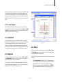
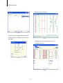
Embedded
etaining Walls
User manual
Software for
Architecture,
Engineering and
Construction
Embedded
Retaining Walls
User manual
www.cype.com
CYPE Ingenieros, S.A.
Avda. Eusebio Sempere, 5
03003 Alicante
Tel. (+34) 965 92 25 50
Fax (+34) 965 12 49 50
[email protected]
www.cype.com
II
Soil Retention Elements
IMPORTANT: PLEASE READ THIS TEXT CAREFULLY
The information contained within this document is the property of CYPE Ingenieros, S.A. and cannot be reproduced nor transfered in its entirety or partially in any
way or means, whether it is mechanically or electronically, for any purpose, without the previous written authorization of CYPE Ingenieros, S.A. The infraction of
property rights can constitute a felony charge.
This document and the information within are an integral part of the documentation that accompanies the License for Use of the CYPE Ingenieros, S.A. software
programs, and from which they are inseparable. Consequently, it is held to the same conditions and responsibilities.
Do not forget that you must read, understand and accept the License for Use Contract of the software that this documentation is part of, before beginning the use of
any component of this product. If you do NOT accept the terms of the License for Use Contract, return the software and all the elements that accompany it to the
place where it was purchased to obtain a full refund.
This Manual corresponds to the version of the software denominated by CYPE Ingenieros, S.A. as Soil Retention Elements (Embedded Retaining Walls). The information contained within this document describes the characteristics and methods for the use of the program or programs that accompany it. The information
within this document may have been modified after the mechanical edition of this book without prior notice. The software that accompanies this document may
have been modified without prior notice.
CYPE Ingenieros S.A. has other services available, such as program Updates, that will allow you to get the latest versions of the software and the corresponding documentation. If you have any questions regarding this text, the License for Use Contract of the software, or other inquiries, please contact your Local Authorized
Dealer or CYPE Ingenieros S.A. at: www.cype.com
© CYPE Ingenieros S.A. (Registered in the European Community)
Edited and printed in Alicante (Spain)
Windows© is the registered trademark of Microsoft Corporation©
CYPE
Embedded Retaining Walls
Table of Contents
1. Calculations ....................................................................... 7
2.1.2.1.
2.1.2.2.
2.1.2.3.
2.1.2.4.
1.1. Analysis Model ..................................................................... 7
1.2. Lateral Pressures ................................................................. 7
Building .................................................................
Adjacent property .................................................
Soil .........................................................................
Information ............................................................
15
15
15
16
1.2.1.Seismic Analysis ............................................................ 9
2.2. Work mode ......................................................................... 16
1.3. Reinforcement Code Checks ............................................. 9
2.3. Program menus ................................................................. 16
1.3.1. Check for combined flexure and axial load .............. 10
2.3.1. F1 Key ......................................................................... 16
1.3.2. Check for shear .......................................................... 10
2.3.2. Question mark icon .................................................... 16
1.3.3. Check for the horizontal stiffeners ............................ 10
2.3.3. Quick Guide ................................................................ 17
1.3.4. Check for the vertical stiffeners ................................. 10
2.4. Assistant ............................................................................. 17
1.4. Design of the reinforcement ............................................. 10
2.5. Reports ............................................................................... 17
1.4.1. Design of the vertical reinforcement ......................... 10
2.6. Plans .................................................................................. 17
1.4.2. Design of the horizontal reinforcement .................... 10
1.4.3. Design of the stiffeners .............................................. 10
3. Earth pressure calculations ............................................ 18
1.5. Design of secant pile walls ............................................... 11
3.1. Introduction ....................................................................... 19
1.6. Design of sheet pile walls ................................................. 11
3.2. Static earth pressure ......................................................... 19
1.6.1. Stress with slenderness factor .................................. 11
3.2.1. Calculation of the active pressure ............................ 19
1.6.2. Stress with top of wall load eccentricity ................... 11
3.2.2. Calculation of the passive pressure .......................... 20
1.6.3. Slenderness ................................................................ 11
3.2.3. Calculation of the ‘at rest’ pressure .......................... 20
3.2.4. Pressure from loads situated on the ground ............
3.2.4.1. Pressures produced by a uniformly
distributed load ...................................................................
3.2.4.2. Pressures produced by a band load
parallel to the top of the wall .............................................
3.2.4.3. Pressures produced by a line load
parallel to the top of the wall .............................................
3.2.4.4. Pressures produced by a point or
concentrated load in reduced areas (footings) ................
3.2.4.5. Pressures from the ‘top of wall’ loads .................
1.7. Design of Mini pile walls .................................................... 11
2. Program Description ....................................................... 12
2.1. Assistants ........................................................................... 12
2.1.1. Assistant 1. Reinforced concrete slurry wall
for buildings ...........................................................................
2.1.1.1. General data .........................................................
2.1.1.2. Soil .........................................................................
2.1.1.3. Intermediate stages of excavation ......................
2.1.1.4. Floor slabs (construction phases) .......................
2.1.1.5. Service phase (finished job) ................................
13
13
13
13
14
14
20
20
21
21
21
22
3.3. Dynamic earth pressure .................................................... 22
3.3.1. Calculation of the active pressure ............................ 22
3.3.1.1. Coefficient of active pressure in dynamic
conditions ........................................................................... 22
2.1.2. Assistant 2. Reinforced concrete slurry walls
for buildings of one or two basements ................................ 14
CYPE
III
IV
Soil Retention Elements
3.3.1.2. Wall-soil friction angle ..........................................
3.3.1.3. Specific weight .....................................................
3.3.1.4. Pressure from groundwater .................................
3.3.1.5. Effects of the loads and surcharge
in the exterior ......................................................................
23
23
23
23
3.3.2. Calculation of the passive pressure .......................... 23
3.3.2.1. Specific weight ..................................................... 23
4. Questions and Answers ................................................. 24
CYPE
Embedded Retaining Walls
Soil Retention Elements
Embedded Retaining Walls
5
6
Soil Retention Elements
CYPE
Embedded Retaining Walls
1. Calculations
Very Important
1.1. Analysis Model
Be aware that the program analyzes the embedded retaining walls as structural elements subjected to the lateral
pressures of the different soils and exterior loads applied
to them.
The analysis model employed consists of a vertical bar
whose mechanical properties are obtained by transverse
linear foot of wall. On this wall acts: the soil, in the exterior
as well as the interior, the loads on the ground, the lateral
support elements such as struts, active anchors, passive
anchors, or construction elements like floor slabs, and the
loads applied at the top of the wall.
Geotechnical calculations, such as the determination of
the end bearing resistance, frictional resistance, groundwater flow, etc., are not carried out and they must be the subject of an accompanying study based on the Geotechnical
report. The same applies for elements like braces or struts,
type of anchor, its diameter, anchorage length, etc., which
also require a separate study.
The introduction of lateral support elements such as
struts, active anchors and passive anchors, establish
exterior conditions on the wall, which are modelled as
springs with the same stiffness as the axial stiffness of the
element.
When a rock layer is introduced, the program considers
the wall fixed if it is embedded into the layer for a length
equal to or greater than two times the wall thickness. Between 8 in. and two times the thickness, the wall is considered to be simply supported by such layer, that is, rotation
is allowed but displacement is restrained.
The discretization of the wall is carried out every 10 in.,
obtaining the soil behavior diagram at each point. Furthermore, the model also includes the points at which the
lateral supports act.
1.2. Lateral Pressures
The lateral pressures that the soil exerts on the wall
depend on the wall’s movement. To take this interaction
into account, the program makes use of soil behavior
diagrams like the one shown in the following figure:
CYPE
7
8
Soil Retention Elements
mally, if a geotechnical study has been carried out, it must
provide the exact value of this modulus for the dimensions
that the wall will have.
These Subgrade Moduli come to represent the stiffness of
the soil at a given point, and may differ according to the direction of the displacement.
In addition, since the stiffness of the soil tends to increase
with depth, a linear variation may be considered, known as
the Gradient Subgrade Modulus, which the user introduces
as the increment of the modulus per foot of depth.
In this diagram, the soil is considered to behave plastically,
in a way that between one phase and the next, the diagram
is updated. The figure below shows this concept, where
δpre is the displacement of the previous phase:
Fig. 1.1
The critical points in the graph, ea, ep, and eo, are the
known active, passive, and at rest pressures, respectively.
The active and passive displacement limits are represented
by δa and δp. These displacements are obtained through
the active and passive Subgrade Moduli introduced by the
user.
The program calculates the coefficients of earth pressure
based on the following formulations:
- At rest earth pressure: Jaky formulation
- Active earth pressure: Coulomb formulation
Fig. 1.2
- Passive earth pressure: Rankine formulation
To obtain information on the calculation of these pressures,
consult the Earth pressure calculations in section 3.
The values for the Subgrade Modulus, like any geotechnical
parameter, are difficult to estimate. In the program, some
guiding values are given for several types of soils, but it is
recommended that specialized literature and empirical data
from soil tests be consulted for more accurate values. Nor-
CYPE
If the wall continues to displace to the right, a point is obtained which moves on the load branch; while if its displacement changes direction, the pressure will vary along
the unloading branch, which passes through the initial point.
At the points where the soil exists on both the exterior and
the interior, the behavior diagram employed is obtained by
adding the corresponding diagrams at that depth on either
side of the wall.
Embedded Retaining Walls
1.3. Reinforcement Code Checks
The procedure for checking the Code provisions applicable to the reinforcement is as follows: first, the geometric
and strength criteria are verified for the horizontal and vertical reinforcement. Then, the stiffeners are checked.
Geometric criteria include concrete cover, spacing limits,
and minimum and maximum reinforcement ratios. Strength
criteria follow the requirements for shear, combined bending and axial force, mechanical reinforcement ratios, and
lap splice lengths. For more information, please see the
Code checks report notes and the corresponding articles
in the Code.
Fig. 1.3
For the strength checks, the program establishes sections
to verify every foot. In each one of the sections, the design
forces are obtained based on the results of each phase
and according to the following cases:
1.2.1.Seismic Analysis
Seismic action makes the pressures on the wall increase
periodically.
- C1: Axial, shear, and bending moment, multiplied by
the load factor.
The active pressure in seismic conditions is greater than
the corresponding one for the static situation.
- C2: Shear and bending moment, multiplied by the load
factor, with no axial force.
Similarly, the passive pressure that the wall can exert on the
soil may be reduced considerably during seismic events.
For the checks of ultimate limit states, the program applies
the load factor introduced by the user, which is a function of
whether the phase is a construction or service phase.
To evaluate these pressures, a pseudo-static method has
been employed with the coefficients of dynamic pressures
based on the Mononobe-Okabe equations. For more information, please consult the Earth pressure calculations
in section 3.
The forces are always calculated by panel and the Code
checks are carried out with respect to the resistant (effective) area of such panel, as indicated in the following figure.
In the results of each construction phase, two graphs are
shown: the first without seismic action and the second with
seismic action.
Likewise, in the force reports, the results for anchorage elements, etc., both cases appear.
Fig. 1.4
CYPE
9
10
Soil Retention Elements
The next sections expand on some of the critical checks as
well as those that the program verifies in addition to the
Code requirements.
1.3.1. Check for combined flexure and axial load
distributed along the whole height of the wall, and the spacing is equal to or less than 8 ft.
These criteria have been extracted from the NTE (Spanish
Technological Standards for Buildings), Soil Preparation,
Foundations.
The check for section strength (design strength) is carried
out using as a constitutive law the stress-strain diagram
with the simplified rectangle compression block. With this
principle, the program can also differentiate zones of
cracked concrete sections, due to combined forces, from
uncracked sections.
1.3.4. Check for the vertical stiffeners
The combined flexure and axial load check is implemented
for all the Codes that the program allows for with their own
peculiarities with respect to compatibility formulations and
strains permitted for the materials that make up the section
(steel and concrete).
1.4. Design of the reinforcement
When the check is carried out, the program makes sure
that the reinforcement is anchored properly to be able to
consider them in the combined forces calculation.
1.3.2. Check for shear
The check for this ultimate limit state is carried out, as with
the combined flexure and axial load case, at different
heights of the wall. Since the wall has no transverse reinforcement, only the contribution of the concrete is considered for resisting shear forces.
The contribution of the concrete against shear is taken from
the term Vc, which is obtained from the simple empirical formula stipulated by the Code. This term is a function of the
concrete strength and the width and effective depth of the
section.
1.3.3. Check for the horizontal stiffeners
The program verifies that: the diameter of the stiffener is at
least equal to the base reinforcement, they are uniformly
CYPE
The same checks as for the horizontal stiffeners apply, but
the spacing of the vertical stiffeners must be equal to or
less than 5 ft.
1.4.1. Design of the vertical reinforcement
From the total entries in the reinforcement table, the most
economic of all the ones that comply with the Code requirements for strength, reinforcement ratios, spacing, etc.,
is selected. The base reinforcement, in addition to adhering
to the spacing and minimum ratio criteria, must cover at
least 50% of the zones where the maximum moment occurs. In those regions where the base reinforcement does
not pass the checks, strengthening bars are provided.
In the cases where the bar lengths are greater than those introduced by the user, the required lap splices are generated.
1.4.2. Design of the horizontal reinforcement
From all the entries in the reinforcement table, the program
selects the most economical from those that meet the spacing and quantity criteria described previously in section 1.3.
1.4.3. Design of the stiffeners
The diameter of the stiffener bar, vertical as well as horizontal, must be equal to or greater than the largest diameter
Embedded Retaining Walls
product of the axial load at the top of the wall and the maximum eccentricity produced by the deformation of the wall.
used in either the exterior or interior face. A number of bars
are provided so that the spacing of the horizontal stiffeners
is at most 8 ft., and 5 ft. for the vertical stiffeners.
1.6.3. Slenderness
1.5. Design of secant pile walls
The slenderness must not be greater than the value recommended by the Code when the element is subject to compression forces.
The design of reinforced concrete secant pile walls follows
the same procedure as for slurry walls. All the reinforcement Code Checks listed in section 1.3 apply except for
stiffeners which are not used in this type of walls.
1.7. Design of Mini pile walls
Mini pile walls are cylindrical elements, drilled on site, reinforced with steel tubing and filled with grout or cement mortar, and whose diameters do not usually surpass 12 in. The
user must define the exterior diameter or the excavation diameter, and the program selects the cylindrical steel tube
from those defined in the library. The design of the Mini pile
follows from combined flexure and axial loads. For the calculation of the concrete section in ultimate limit states, the
program uses the strain compatibility method, with the corresponding concrete and steel stress-strain diagrams. Beginning with the section chosen for the job, all the sections
in the series are checked in sequence. A minimum or accidental eccentricity is considered, as well as the buckling eccentricity based on the Code, limiting the value of the
mechanical slenderness, also as indicated by the Code.
1.6. Design of sheet pile walls
Once a series and a profile within the series have been chosen, the design may proceed. In the case that the profile
does not meet the strength requirements, the program
places the next section in the series and analyzes the wall
again, since the stresses also change when the profile
changes. Next, the check is run once more, and if the new
section does not pass either, then the process is repeated.
The checks made on this type of wall are the following:
1.6.1. Stress with slenderness factor
Von Misses stress calculated from the normal stress (a
function of the axial force, effective length due to the slenderness, bending moment, and the section modulus) and
the tangent stress (a function of the shear force and the resisting shear area).
The effective length considered is the clear distance in each
phase, taking into account that the embedded portion is
fixed, or the distance between points of zero moment
(when there are floor slabs, struts, etc., that produce inflection points in the bending moment diagram).
1.6.2. Stress with top of wall load eccentricity
The maximum size of the circular tube is limited to the
diameter of the Mini pile.
In this case, rather than multiplying the axial force by the effective length factor as in the previous situation, the program considers the additional moment calculated from the
CYPE
11
12
Soil Retention Elements
2. Program Description
Fig. 2.1
2.1. Assistants
When creating a new job, the Assistant Selection dialogue will open.
Fig. 2.2
CYPE
Embedded Retaining Walls
2.1.1.1. General data
If you create a new job with an Assistant, the program generates the data necessary to describe it, depending on the
type of Assistant selected, using a minimum number of parameters introduced in sequence. It includes the generation
of the construction process and the pre-dimensioning of
the geometry of a reinforced concrete slurry wall - excavated by phases with successive bracing (temporary or permanent). A wall that supports the various floors at the
different heights while considering the possibility of having
adjacent structures. It will also generate the final service
stage in which the wall is able to support the load of a building. Any data generated can be reviewed and/or modified
after the job has been created.
One must indicate the total depth of the excavation.
The pre-dimensioning of the wall thickness is H/20 (where
H is the excavation depth), with a minimum of 18 in. and a
maximum of 42 in. Rounding occurs to values of 18, 24, 32,
and 42.
Fig. 2.3
2.1.1.2. Soil
The total height of the wall varies between 2H and 1.4H, depending on whether the excavation is braced or not. A value within that range is chosen based on the number of
excavation phases. If rock exists at a shallower depth, the
wall will be embedded 4 in. into the layer; this is the minimum value to consider the wall simply supported at that
point.
There is the possibility of introducing ground water, rock,
and a surcharge on the ground in the exterior. In addition,
one must configure the different soil layers found.
To understand the approximations made, read the help windows for every dialogue of the Assistant.
There are two types of Assistants:
2.1.1. Assistant 1. Reinforced concrete
slurry wall for buildings
Fig. 2.4
Assistant for the generation of walls of various levels. Data
entry dialogues appear successively and their options contain on-screen help through the question mark icon. Note
that when an “elevation” is called for, one must introduce a
negative sign since the program takes the ground surface
as elevation 0'-0".
2.1.1.3. Intermediate stages of excavation
One must define the number of excavation stages in which
anchors are placed, and for each, the elevation and type of
CYPE
13
14
Soil Retention Elements
anchor (strut, permanent or provisional active anchor, permanent or provisional passive anchor). The anchor has its
own elevation.
For each excavation stage, the Assistant generates 2 phases. The first is the excavation of the ground, and the second
is the placement of the anchorage. The elevations of the excavation stages cannot be greater than the value of the total
excavation depth indicated in the first window of the Assistant, General data. If, for example, the total depth of the excavation is 30 ft. and its excavation stages are of 10ft., only
two stages need to be defined: the first, at the elevation
-10 ft., and the second at -20 ft. The program automatically
generates the last excavation stage without an anchorage
phase.
Fig. 2.6
2.1.1.5. Service phase (finished job)
One may introduce the loads at the top of the wall, if any,
and the service phase shears that the basement floors
transfer to the wall.
Fig. 2.5
2.1.1.4. Floor slabs (construction phases)
This is the list of floors and foundation (if this exerts an anchorage type effect), indicating their top elevation, depth
(thickness), and shear load (in lbs/ft) in the construction
phase. Meaning that the slab on grade or mat foundation
must also be defined. The top elevation of the foundation
minus its depth must coincide with the elevation of the bottom of the excavation, in this case: -50 ft. - 3 ft. = -53 ft.
Fig. 2.7
2.1.2. Assistant 2. Reinforced concrete
slurry walls for buildings of one or two
basements
Just as with the previous Assistant, successive data entry
dialogues appear.
CYPE
Embedded Retaining Walls
2.1.2.2. Adjacent property
Type of adjacent property (no adjacent structures, road
with light traffic, road with heavy traffic, or adjacent building
for which one must define the number of floors and the average height of its foundation). Based on the selection, a
surface load will be applied on the ground in the exterior.
Fig. 2.8
2.1.2.1. Building
By default, one starts with one basement; if the corresponding box is activated, a sub-basement may be established. One must indicate the clear heights between floors,
transverse spans (free span of the floors between the wall
and the next support; with this data the program will approximate the depths of the floor slabs and the loads that
they transmit to the wall), whether the building is supported
by the wall (indicating the number of floors above ground
level), and, lastly, the type of foundation. With this last entry,
one informs the Assistant of the type of foundation for the
building.
Fig. 2.10
2.1.2.3. Soil
A maximum of two layers are allowed. One can also define
whether a rock layer or groundwater exists, indicating their
respective depths.
Fig. 2.9
Fig. 2.11
CYPE
15
16
Soil Retention Elements
2.1.2.4. Information
Before creating the job, a list appears with all the data
entered and approximations made. At this point, one may
still go back and make changes, or otherwise wait for the
program to finish creating the job. This list can be printed
or exported to HTML, PDF, TXT, and RTF.
6. Review the Code checks report by clicking on the button with the same name.
7. Edit the reinforcement, if necessary, with the Reinforcement Editor, and verify the Code requirements once
more with the Code checks button.
8. Obtain the job reports and plans by using the Job Reports and Job Plans buttons respectively.
2.3. Program menus
The program menus and the dialogues that open when executing certain options have on-screen help available.
This help can be acquired in three different ways:
2.3.1. F1 Key
To obtain help about a menu option, place the cursor over
the menu option and, without clicking on it, press the F1 key.
Fig. 2.12
2.2. Work mode
2.3.2. Question mark icon
The following steps are recommended:
1. Create a New file with the name of the job.
2. Select the type of Assistant or rather, None. In the latter
case, one must create the construction phases or stages manually with the Selection button and indicate all
the data necessary for each phase: depth of excavation, anchors, etc.
3. Review the data introduced, browsing through the
phase selection.
4. Calculate and review the forces for each phase by clicking on the Forces button.
5. If the wall is a reinforced concrete slurry wall, click on the
Design button to obtain the reinforcement.
CYPE
On the menu bar of the program’s main window there is an
icon with a question mark. You can obtain help about a
specific program option in the following way: click on the
icon; scroll down the desired menu option and place the
cursor over the command for which you would like help;
click on that command. Having done this, a window will appear with the desired help.
To deactivate this type of help, you can do one of the following: click on the right mouse button, click on the question mark icon, or press the Esc key. One can also obtain
help on the toolbar icons. To do this, click on the question
mark icon. By browsing through the icons, a blue outline
will appear on those icons for which help is available. Next,
click on the desired icon to open the help window.
Embedded Retaining Walls
There also exists a question mark icon on the title bar of the
dialogues that are opened when selecting a program option. When clicking on this icon and browsing through the
dialogue window, the options that contain help will be highlighted in blue. Click on those options to open the help window.
2.3.3. Quick Guide
The information related to the menu options can also be
viewed and printed by choosing the option Help > Quick
Guide. The quick guide does not list information on the usage and options of the dialogues.
2.4. Assistant
When creating a new job, one has the option of using an
Assistant that will generate the data necessary to describe
the wall using a reduced number of parameters in sequence. It includes the pre-dimensioning of the geometry
and the generation of loads. Any data generated can be reviewed and/or modified once the job has been created.
Fig. 2.13
2.6. Plans
The way to obtain job reports is through the File > Print
> Job Plans option or the plotter icon on the upper right
hand corner of the main window.
2.5. Reports
The following operations can be carried out for the drawing
of plans:
The way to obtain job reports is through the File > Print
> Job Reports option or the printer icon on the upper
right hand corner of the main window.
- The Plan selection window (Fig. 2.14) allows adding
one or various plans to print simultaneously and specify the peripheral of choice: printer, plotter, DXF, or
DWG; one may also select a title block (from CYPE or
any other defined by the user), and configure the layers.
The reports can be directed to a printer (with an optional
print preview, page adjustment, etc.) or one can generate
HTML, PDF, TXT, and RTF files (Fig. 2.13).
CYPE
17
18
Soil Retention Elements
- Modify the position of the texts.
Fig. 2.14
- In each plan, one can configure the elements to print,
with the possibility of including previously imported
user details.
Fig. 2.16
- Change the layout of the objects within the plan or
move them to another.
Fig. 2.15
Fig. 2.17
CYPE
Embedded Retaining Walls
3. Earth pressure calculations
3.1. Introduction
γ 'partial = γ ' + ( γ − γ ' ) · 1 − 100 − x 
100 

The lateral earth pressures on a wall can be of the following
types:
The program considers the infiltrated water along the
whole height of the wall.
• Active pressure. The soil exerts a pressure on the
wall allowing enough deformations in the direction of the
push to take the soil to a state of failure. This is the typical case when a soil ‘action’ is developed.
• Percentage of passive pressure (only in cantilever or basement walls). Expressed as a % over the
passive pressure value.
• At rest pressure. The soil exerts a pressure, but the
wall does not suffer considerable deformations, that is,
they are null or negligible. The value of the pressure is
greater than the active.
• Elevation of passive pressure (only in cantilever
or basement walls). Elevation below which passive
pressure is considered (0 by default; then it will only act
in the footing, if passive pressure is considered).
• Passive pressure. When the wall displaces against
the soil, the soil is compressed and it reacts. This situation is always a ‘reaction’. Its value is much greater than
the active.
• Rock. Activating this option permits defining a rock layer, for which one must indicate the elevation, and this
must be lower than the fill elevation. From the rock elevation down, all earth pressures are annulled, save for
the hydrostatic pressures.
The parameters that characterize a layer of soil or fill are:
• Water table. Above such level, the soil is considered
with its apparent unit weight γ or with the unit weight of
the partially saturated soil if the percentage of drainage
loss is under 100%. Below the water table, the submerged unit weight γ’ is used, additive to the hydrostatic pressure to obtain total lateral pressures.
β). Expressed in degrees with respect to
• Slope angle (β
the horizontal. Its limit is the internal friction angle.
• Apparent unit weight (γγ). Also called the dry unit
weight.
• Submerged unit weight: (γγ’). The unit weight of the
soil below the water table.
ϕ). Intrinsic soil property that
• Internal friction angle (ϕ
describes the maximum natural slope angle at which
failure will not occur.
3.2. Static earth pressure
3.2.1. Calculation of the active pressure
• Drainage loss (only in cantilever or basement
walls). Expressed as a %, allows the consideration of
infiltrated water in the soil that increases the lateral pressure as an additional fraction of the hydrostatic pressure and the partially saturated unit weight. A value X%
will produce a hydrostatic pressure of (100 - X) % and
an earth pressure according to the following unit weight:
The active pressure is resolved by applying Coulomb’s
theory.
The values of the horizontal and vertical pressures in a
point of the exterior located at a depth ‘z’ are calculated
with:
CYPE
19
20
Soil Retention Elements
3.2.3. Calculation of the ‘at rest’ pressure
p h = γ ⋅ z ⋅ λh ; pv = γ ⋅ z ⋅ λ v
The ‘at rest’ pressure is resolved by applying Jaky’s theory.
It is calculated as:
where:
λ h=
sin2 ( α + ϕ )

sin ( ϕ + δ ) · sin ( ϕ − β ) 

sin2α · 1 +
sin (α − δ ) · sin (α + β ) 



2
prest = γ ⋅ z ⋅ Krest
=
where:
Krest = 1− sin ϕ
z: depth
γ: unit weight of the soil
ϕ: internal friction angle of the soil
λ v = λh ⋅ cot g (α − δ)
z: depth
α: angle of the wall face with the horizontal
In the case where there is a slope or embankment, the
complementary formulation of the Corps of Engineers,
1961, is used.
γ: unit weight of the soil
δ: wall-soil friction angle
ϕ: internal friction angle of the soil
β: angle of the slope
3.2.4. Pressure from loads situated on the
ground
When the cohesion of the soil is considered:
ph = γ ⋅ z ⋅ λh − 2 ⋅ c ⋅ λ h ⋅ cos δ
3.2.4.1. Pressures produced by a uniformly
distributed load
where:
Coulomb’s method is applied and the horizontal and vertical pressures produced by a uniform surcharge equal:
c = cohesion of the soil
3.2.2. Calculation of the passive pressure
The calculation of the passive pressure is similar to the calculation of the active pressure. But one must change the
sign of the internal friction angle in the previous formulas.
Moreover, when the cohesion of the soil is considered:
ph = γ ⋅ z ⋅ λh + 2 ⋅ c ⋅ λh ⋅ cos δ
where:
c = cohesion of the soil
Fig. 2.1
CYPE
Embedded Retaining Walls
3.2.4.3. Pressures produced by a line load
parallel to the top of the wall
sin α
sin α
ph = λ h ⋅ q ⋅
pv = λ v ⋅ q ⋅
sin ( α + β ) ;
sin (α + β )
The method based on Elastic Theory has been employed.
The lateral pressure that a line load q exerts, for the case of
a vertical exterior face and a horizontal ground surface,
equals:
where:
λh: coefficient of horizontal pressure
λv: coefficient of vertical pressure
q: surface load
α: angle of the wall face with the horizontal
β: angle of the slope
3.2.4.2. Pressures produced by a band load
parallel to the top of the wall
The lateral pressure that a band load exerts for the case of
a vertical exterior face and a horizontal ground surface, following Elastic Theory, equals:
Fig. 2.3
pq =
q
sin2 2ω
π⋅z
3.2.4.4. Pressures produced by a point or
concentrated load in reduced areas (footings)
The method based on Elastic Theory has been employed.
The lateral pressure that a point surcharge exerts, for the
case of a vertical exterior face and a horizontal ground surface, equals:
Fig. 2.2
pq =
2⋅q
⋅ (β − sin β ⋅ cos 2ω)
π
If (m < 0.4),
q: band load
pq = 0.28 ·
β and ω: angles as described in the figure. The first in the formula
is measured in radians.
CYPE
q
2
H
·
n2
0.16 + n2 


3
21
22
Soil Retention Elements
If (m ≥ 0.4),
pq = 1.77 ·
q
2
H
·
To evaluate these pressures, a pseudo-static method has
been employed with the coefficients of dynamic pressures
based on the Mononobe-Okabe equations.
m2 n2
m2 + n2 


3
3.3.1. Calculation of the active pressure
3.3.1.1. Coefficient of active pressure in dynamic conditions
The coefficient of active pressure in dynamic conditions is
the following:
K ad =
cos ( α + θ )
⋅ K*
cos θ ⋅ cos α a
where:
α: angle of the wall face with the vertical
θ: angle defined by the following expressions:
 ah 
θ = arctg 

 g − av 
Fig. 2.4
3.2.4.5. Pressures from the ‘top of wall’ loads
One may introduce point loads or a bending moment at the
top of the wall.
These loads generate forces on the wall directly, but they
may also have a passive response from the soil if that is
the case.
 ah
θ = arctg 
 g − av
 γd
⋅ γ'

Case 1
Case 2
where:
g: acceleration due to gravity
γd: dry unit weight
γsat: saturated unit weight
γ’: submerged unit weight
ah: design horizontal acceleration
av: design vertical acceleration, which the program takes as half
of the horizontal
3.3. Dynamic earth pressure
Seismic action makes the pressures on the wall increase
periodically. The active pressure in seismic conditions is
greater than the corresponding one for the static situation.
Similarly, the passive pressure that the wall can exert on the
soil may be reduced considerably during seismic events.
CYPE
K*a the coefficient of active pressure in static conditions, but in its
calculation, α is replaced by (α + θ), and β by (β + θ).
Case 1 corresponds to dry or partially saturated soils in
the exterior, always located above the water table.
Case 2 corresponds to soils below the water table.
Embedded Retaining Walls
3.3.1.2. Wall-soil friction angle
3.3.1.5. Effects of the loads and surcharge in
the exterior
The wall-soil friction angle can decrease considerably during seismic events. This leads to an additional increase of
the active pressure. Therefore, by considering an angle of
0, one remains on the side of safety.
The intensity of the loads on the ground shall be multiplied
by:
a
f = 1+ v
g
where:
3.3.1.3. Specific weight
av: design vertical acceleration = 1/2 · ah
The pressure due to the weight of the soil is greater since
there is an increase in the specific weight of the soil, above
as well as below the water table. The coefficient to apply to
the unit weight, which the program considers automatically,
is:
g: acceleration due to gravity
3.3.2. Calculation of the passive pressure
The passive pressure can decrease during a seismic event.
a
f = 1+ v
g
The coefficient of passive pressure in dynamic conditions
is the following:
where:
K pd =
av: design vertical acceleration = 1/2 · ah
g: acceleration due to gravity
cos (α − θ )
⋅K*
cos θ ⋅ cos α p
where:
α: angle of the wall face with the vertical
3.3.1.4. Pressure from groundwater
θ: the same angle defined for the active pressure case
K*p: the coefficient of passive pressure in static conditions, but in
its calculation, α is replaced by (α - θ), and β by (β - θ).
Below the water table, the increase in pressure at each
point is calculated as:
a
∆E w = 7 ⋅ h ⋅ γ w hz
8 g
3.3.2.1. Specific weight
The pressure due to the weight of the soil is smaller. The
coefficient to apply to the unit weight, which the program
considers automatically, is:
where:
ah: design horizontal acceleration
g: acceleration due to gravity
a
f = 1− v
g
hz: depth
γw: unit weight of water
where:
av: design vertical acceleration = 1/2 · ah
g: acceleration due to gravity
CYPE
23
24
Soil Retention Elements
4. Questions and Answers
For Users in the United States:
Please contact your local Authorized Dealer.
For Users in Europe:
In the web page (http://www.cype.com), in the Technical
Support Section, you can find the link to FAQ, which contains the answers to the most frequently asked questions,
constantly updated, received by the Technical Support
Department of CYPE Ingenieros.
CYPE