Download p500 ver 2.0 user manual

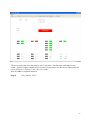
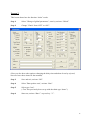
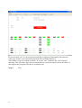
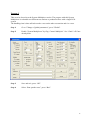
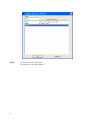
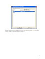
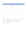
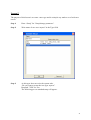
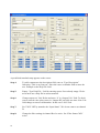
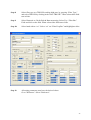
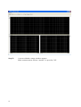
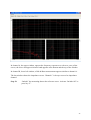
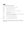
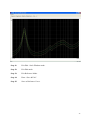
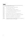
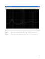
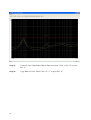
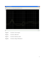
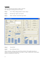
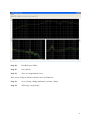
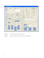
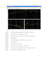
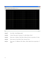
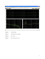
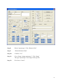
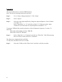
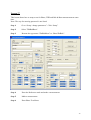
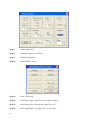
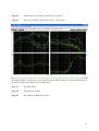
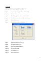
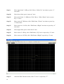
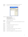
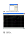
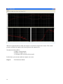
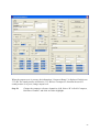
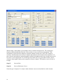
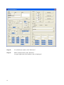
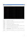
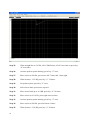
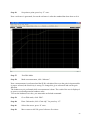
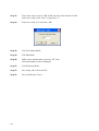
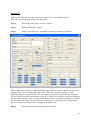
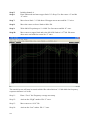
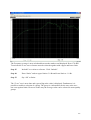
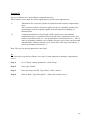
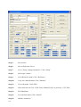
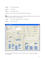
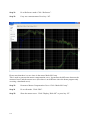
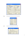
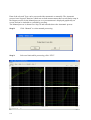
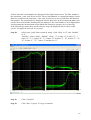
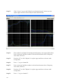
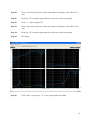
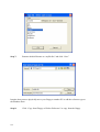
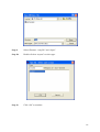
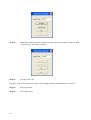
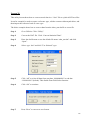
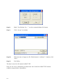
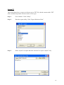
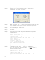
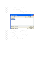
P630 Pro
User Manual
Volume 2
Version Pro 1.2-a
14 December 2007
Volume 2
Getting Started with P630 Pro ....................................................................................................3
Lesson 1 ......................................................................................................................................5
Lesson 2 ....................................................................................................................................11
Lesson 3 ....................................................................................................................................15
Lesson 4 ....................................................................................................................................17
Lesson 5 ....................................................................................................................................21
Lesson 6 ....................................................................................................................................32
Lesson 7 ....................................................................................................................................34
Lesson 8 ....................................................................................................................................42
Lesson 9 ....................................................................................................................................44
Lesson 10 ..................................................................................................................................48
Lesson 11 ..................................................................................................................................50
Lesson 12 ..................................................................................................................................58
Lesson 13 ..................................................................................................................................62
Lesson 14 ..................................................................................................................................64
Lesson 15 ..................................................................................................................................72
Lesson 16 ..................................................................................................................................76
Lesson 17 ..................................................................................................................................79
Lesson 18 ..................................................................................................................................83
Lesson 19 ..................................................................................................................................87
Lesson 20 ..................................................................................................................................91
Lesson 21 ..................................................................................................................................95
Lesson 22 ................................................................................................................................101
Lesson 23 ................................................................................................................................109
Lesson 24 ................................................................................................................................115
Lesson 25 ................................................................................................................................125
Lesson 26 ................................................................................................................................129
Lesson 27 ................................................................................................................................133
1
SURVEY
Lesson 1 – 4
Lesson 5 - 22
Lesson 1
Lesson 2
Lesson 3
Lesson 4
Lesson 5
Lesson 6
Lesson 7
Lesson 8
Lesson 9
Lesson 10
Lesson 11
Lesson 12
Lesson 13
Lesson 14
Lesson 15
Lesson 16
Lesson 17
Lesson 18
Lesson 19
Lesson 20
Lesson 21
Lesson 22
Lesson 23
Lesson 24
Lesson 25
Lesson 26
Lesson 27
2
Are for USERS
Are for TECHNICIANS
First exercise for user. "Run speaker tests".
Same as lesson 1, but shows results as a status flag instead of colour
coded curves.
Same as lesson 2 but extended with the function "Chain".
Exercise in using System Multiplexer.
Setup of new type.
Copy parameters from an existing type to a new type.
Demonstration of Resonance mode.
Demonstration of Scale mode.
Demonstration of Edit/Convert mode.
How a chain function is established.
Making of a compensation curve.
User calibration of a compensation curve.
Delete types.
THD measurements.
Rub & Buzz measurements.
THD and Rub & Buzz measurements.
Phase, THD and Rub & Buzz measurements at same time.
How to use Ambient Noise check.
How to work with Tolerance Files
Demonstration of the output Compressor function
Use of Loudness and adjustment of sensitivity
Use of Sensitivity and Average tests.
Master curve and Master compensation curve.
Utilities 1: Process stored data and make a new reference.
Utilities 2: Copy a reference from one PC to another PC.
Utilities 3: Convert the A4M_STAT.DAT file to ASCII text file.
Utilities 3: Export and import reference to/from ASCII text file.
Getting Started with P630 Pro
To get a quick start, use the demo program “p630prodemo.exe” or the live version
“p630pro.exe”. The “p630prodemo” program is functioning without any P600 hardware.
Start the program by double click on the “p630prodemo” icon or on the file
“p630prodmo.exe”.
Options:
Run
Setup
Global
Utility
Spl
Pw. Mgr.
Hw. Mgr.
Run speaker tests. Operation mode
Setup and change parameters. Technician mode
Change of global parameter. Global setup.
Utility functions. Technical mode
Setup of microphone sensitivity used for Spl scales.
Password Manager.
Hardware manager
In the following we go through all lessons. It is recommended to follow these lessons
sequentially. Not all functions and possibilities are demonstrate, but hopefully adequately for a
solid introduction to the most important parameters and functions.
3
4
Lesson 1
Let us pretend that a number of valid setups previously have been created in technician mode.
From the start-up screen:
Step 1:
Select operator mode by activating “Run”.
The following screen will appear:
Step 2:
A list of "valid types" appears.
Select "demo" and select “Ok”.
5
If a previous type have been called earlier in “run” mode the program check, if the online
statistics is activated, for changes for called “type”. This prevents errors in statistics.
If the same “type” is called or the on-screen statistics is deactivated this warning is not
displayed.
6
Step 3:
Start a measurement, select “Run 1” or pressing key “1”.
If switch "Display Graph By Reject" is activated in global, the measured curves appear. Please
notice that the data curves are changing colour from green to red, where data are rejected. See
channel B. The test results are displayed as green flag for approved and red flag for rejected
test on left and right sides.
Note: U-code is optional function.
7
Step 4:
Activate the cursor by activating "Cursor".
A cursor, an extended cross, appears in Ch. A. Corresponding values of frequency and level are
shown in the upper right corner of the screen. Active channel and cursor focus (upper, lower or
data) are shown in the upper left corner.
Step 5:
Move cursor to the next channel (channel B) by pressing "+".
Step 6:
Zoom in on active channel (channel B) by “Display Zoom In” or by pressing
"Page Up",
8
Activating the arrow-keys can move the cursor. By activating “Move 0 Fast” or pressing "0"
(nil), the cursor moves approx. 10 times faster.
Step 7:
Activate "Exit” to go one menu up.
This full sequence, step 1 - 7, has simulated a typical test sequence. Normally, the operator
uses step 1 - 3 for starting up and then stays in step 3 for successive measurements. Only if a
test is rejected, it can be interesting to search for the reason (step 4 - 6).
Step 8:
Activate "Exit” to exit.
9
10
Lesson 2
This lesson is like lesson 1, but without curve display “ON”.
Step 1:
Go to "Change of global parameter", activate “Global”.
Note: Print is optional.
Step 2:
Unmark “Display Graph By Reject”.
11
Step 3:
Save changes and exit by activate “OK”.
Step 4:
Select “Run speaker tests”, activate “Run”.
Step 5:
Select type “demo”.
Step 6:
Start test, activate “Run 1” or press key “1”.
12
The test sequence has been the same as step 3 in lesson 1, but this time with flags for test
results - green for approved and red for rejected. If you wish to see the curves, identical to the
curves in lesson 1, activate “View” for view result.
Note: U-code is a optional function.
Step 9:
Exit, activate “Exit”.
13
14
Lesson 3
This lesson shows how the function “chain” works.
Step 1:
Select "Change of global parameters", enter by activate “Global”.
Step 2:
Change "Chain" from “OFF” to “ON”.
(Here you also have other options: changing the delay time and abort of test by rejected,
however leave these items for the moment).
Step 3:
Save and exit, activate “OK”.
Step 4:
Select "Run speaker tests", activate “Run”.
Step 5:
Select type "test".
(“Test” has previously been set up with the chain type “demo”).
Step 6:
Start test, activate “Run 1” or press key “"1”.
15
Please note that "test" is carried out and result flag is displayed. Immediately thereafter the
chain type "demo" is activated and carried out and result flag displayed.
The number of types in a chain is infinite. To see the “test” graph use the “first” function.
Warning: Take care that a type does not chains back to a type previously used in the chain. If
this happens the program will work in an infinite loop.
Step 7:
16
Exit.
Lesson 4
This exercise shows how the System Multiplexer works. The purpose with this System
Multiplexer is to handle two different test stations or production lines with a single P630
system.
The handling time is thus utilised to make a test on the other test station and vice versa.
Step 1:
Go to "Change of global parameters", press "Global".
Step 2:
Enable "System Multiplexer" by flag “Control Multiplex”. Set “Chain” off if not
already done.
Step 3:
Save and exit, press “OK”.
Step 4:
Select “Run speaker tests”, press “Run”.
17
Step 5:
18
For system 1 select type "test".
For system 2 select type "demo".
Now the multiplexer system 1 will carry out type "test" each time system 1, "1", is activated,
and type "demo" by activating system 2, pressing "2".
19
Step 6:
Activate “Run 1” or press key “1” for start of test system 1.
Step 7:
Activate “Run 2” or press key “2” for start of test system 2.
Step 8:
Exit Run Mode”.
20
Lesson 5
The purpose of this lesson is to create a new type and in a simple way make a set of reference
curves.
Step 1:
Enter “Setup” for "Setup/change parameter".
Step 2:
Write name of new test “mytest” in the Type field.
Step 3:
As this type does not exist, the system asks:
“Do you want to create the new type: mytest”.
Respond, "YES" for Yes.
The following pre-set standard setup will appear:
21
A predefined standard setup appears on the screen.
Step 4:
To add a comment to the description field, enter at “Type Description”
following: "This is my first test". Place the curser on another field to enter the
text. Example on the Help File field.
Step 5:
Empty “Type Help File “ field by entering spaces if not already empty. We do
not want to use a help file in current moment.
Step 6:
Change output to 6 Volt. Delete and enter “6” in “Output Volt” field. To check
correct entered value place cursor in “Output dB” and click one time. Note Volt
field change to nearest valid number. In this case 5.9992 Volt.
Step 7:
Set "Ch D" OFF by unmarks the “Input Status”. We do not want to use channel
D.
Step 8:
Change the filter settings in channel B to be active. Set “Filter Status Ch B”
active.
22
Step 8:
Select filter type to a TRK-HP, tracking high pass, by pressing “Filter Type”
and select TRK-HP by clicking in the field “TRK-HP”. When selected the field
turn to blue.
Step 9:
Select Harmonic to 5th for Rub & Buzz measuring. Select 5 by “Filter Har.”
Field and click on the field. When selected the field turn to blue.
Step 10:
Select band with to “oo”. Select “oo” on “Filter Freq/Bw” and highlight to blue.
Step 11:
All testing parameters now have the desired values.
Go to "Reference". Select "Reference".
23
Step 12:
24
A screen with three empty windows appears.
Make a measurement, activate “measure” or press key "M".
In channel A, the upper window, appears the frequency response as a red curve, two yellow
curves, the lower and upper tolerance band appears at the bottom and the top of the window.
In channel B, lower left window, a Rub & Buzz measurement appears similar to channel A.
The last window shows the impedance curves. Channel C is always reserved as impedance
channel.
Step 13:
“Include” the measuring data to the reference curve. Activate “Include All” or
press key “I”.
25
The red measuring curve is now concealed behind two identical yellow upper and lower
reference curves. By carrying out more measurements an envelope curve is formed by
including each "good" measurement.
A number of “good” speakers can thus provide the basis for the reference curves.
Step 14:
To further elaborate on the reference curves go to "Edit mode", activate "Edit"
or press key “E”.
Step 15:
Check that the cursor is on "Ch A upper (reference curve)", if not, press “arrow
up” until cursor is there.
Step 16:
Activate "Fast cursor", by “Move, 0 Fast” or press key “0”, “nil” (this makes
the cursor go ten times faster than normally).
26
Step 17:
Move upper reference curve 3.1 dB up. Activate “Move, 9 Move Up” or press
key "9" twice. Using the numeric keyboard on the right of the keyboard makes
this work easier.
Step 18:
Move cursor to "Ch A lower (reference curve)". Press once on “arrow up”.
Step19:
Move lower reference curve -3,1 dB down. Activate “Move, 3 Down” or press
key “3” twice.
Next we want to move the entire envelope curve between 1474,0 - 3388.0 Hz -3,1 dB
Step 20:
Move cursor to 1474.0 Hz. Press “right arrow” three times.
Step 21:
Move the point 1474.0 Hz -3,1 dB down. Activate “Edit, Point 2 Down” or
press key “2”" twice.
Step 22:
Press <CTL> “arrow right” three times or activate “Move, Move Part Right”
tree times.
27
Next, move the entire envelope curve between 3388.0 Hz - 1474.0 Hz +3,1 dB.
Step 23:
Move cursor to upper reference curve. Press “arrow down” once.
Step 24:
Move the point 3388.0 Hz 3,1 dB up. Activate “Edit Point, 8 Up” or press key
“8” twice.
Step 25:
Press <CTL> “arrow left” three times or activate “Move, Move Part Left” tree
times.
28
Step 26:
Go to channel B. Press "+" once and the cursor moves to the next window,
channel B.
Step 27:
Move upper reference curve 4,7 dB up. Activate by “Move, 9 Move Up” or
press key "9" three times.
Step 28:
Reset lower reference curve. Press <CTL> “page down”.
29
Step 29:
Go to the impedance channel "Ch C". Press "+" once and the cursor moves to
the next window, channel C.
Step 30:
Move lower reference curve -2.0 dB down. Activate by “Move, 3 Move Down”
or press key "3" twice.
Step 31:
Move cursor to upper reference curve. Press “arrow down” once.
Step 32:
Move upper curve 2.0 dB up. Activate by “Move, 9 Move Up” or press key "9"
twice.
Step 33:
Everything is now ready for test. Exit.
30
Step 34:
Leave "Reference mode". Exit.
Step 35:
The whole setup is now ready to store. Activate "Save & exit".
Step 36:
Save setup as “Reference curve”. Activate “Save as Reference Curve”.
Step 37:
Now "mytest" is ready to be used. Go to "Run" and test type “mytest” (see
lesson 2).
31
Lesson 6
This exercise shows how an existing type setup is copied to another or a new type.
Note: The step for entering password is not listed.
Step 1:
Go to “Setup / change parameter” activate “Setup”.
Step 2:
Select the type "mytest" (see lesson 5).
Step 3:
Enter "mytestcopy" in field “Type Name”.
Note that when Name is changed the Description field is cleared.
Step 4:
Enter new description “my new copy of mytest” in field “Type Description”
Step 5:
Enable polarity test at 5 mSec. if not already done.
Step 6:
Save new setup by “Save & Exit”.
32
Step 7:
Save setup as “Save as Reference Curve”.
Remark:
Normally there is only little direct use for copying a type to a new type, but this
feature is very useful when you only have a few corrections from a previously
setup type. The corrections are made between step 3 and step 4.
33
Lesson 7
This lesson shows how to install a resonance test.
Note: The step for entering password is not listed.
Step 1:
Enter “Setup / change parameters” activate “Setup”.
Step 2:
Establish new type wit name “resonance”.
Step 3:
“Create new type,” press “YES”.
Step 4:
Write “Example of Rs, Q, F, & EBP” in field “Type Description”.
Step 5:
Set output to 2 Volt.
Reset field “Output Volt” and enter “2”.
Step 6:
Disable Polarity Test. Unmark “Sensitivity Test, On” of not already unmarked.
(This test is not to be used in this example).
Step 7:
Set “Ch A” OFF by unmark “Input Status Ch A”.
Step 8:
Set “Ch B” OFF by unmark “Input Status Ch B”.
Step 9:
Set “Ch D” OFF by unmark “Input Status Ch D”.
The channel C is always the impedance channel. If you want to carry out an impedance
measurement, fres, Q and F, this channel must be "ON". Make sure Rs = 0.1. Select Rs with
Gain field in Ch C.
34
Step 10:
Go to “Reference settings” by clicking on “Reference”.
Step 11:
Carry out a measurement. Click on “Measure” or press key “M”.
35
Step 12:
Include measured data to the reference curve. Click on “Include” or press key
“I”.
Step 13:
Include channel C by clicking on “Channel C”.
Step 14:
Go to “Edit mode” by “Edit” or press key “E”.
Step 15:
Activate “Fast cursor”. Press key “0”, once or use “Move, 0 Fast”.
Step 16:
Cursor is active on upper reference curve.
Move upper reference curve + 1 dB up. Press "9" once or “Move, 9 Move Up”.
Step 17:
Move cursor to lower reference curve. Press “arrow up” once.
Step 18:
Move lower reference curve -1 dB down. Press "3" once or “Move, 3 Move
Down”.
Step 19:
Refresh display. Press "Page Down" once.
If you anytime want to update the graphic display, press "Page up" or "Page Down".
Step 20:
36
Go to "Resonance test". Click on “R-test” or press key “R”.
Step 21:
Activate “Fast cursor”. Press key “0” once.
Step 22:
Move cursor towards 47,2 Hz by using left arrow. Deactivate fast cursor by
pressing “0”, nil.
Make the final movements using left or right arrow.
To carry out a resonance test the upper and lower frequency must be selected. The resonance
frequency must be between these. This test is carried out in "run mode". By "opening" the
reference curve between upper and lower test frequency and by placing the tolerance band
appropriate, the following tests are made:
a.
b.
c.
Test resonance between lower and upper values.
Test Q for upper limit.
Using the factor F = fres/Q:
Test Q for lower limit and check factor F.
If the curve between "low" and "high" test frequencies is outside, but accepted with the upper
and lower reference curves, this part of the curve is changing into red, "rejected".
These tests are always carried out when "low" and "high" frequencies are active. If you don't
want the test, reset freq. by “Reset” or key “4”.
Step 23:
Set "Low freq" by selecting “Low” or press key “1” (frequency is at 47.2 Hz).
37
A brown dot-and-dash line appears.
Step 24:
Move cursor to 91,9 Hz by using right arrow.
Step 25:
Set "High freq" by selecting “High” or press key “2”.
A brown dotted line appears at 91.1 Hz.
Step 26:
Enter Q Set menu by enter “Q-Set” or press key “Q”.
38
Step 27:
Select Q test: Qms - Approximation at –3dB level (default).
Step 28:
Select Q test upper limit to 4.0.
Step 29:
Select Q test lower limit to 2.1 and press “OK”.
Step 30:
Enter F Set menu by enter “F-Set” or press key “F”.
Step 31:
Select F test upper limit to 25.0 hertz.
Step 32:
Select F test lower limit to 17.2 hertz and press “OK”.
Step 33:
Enter EBP menu by enter “EBP”.
Step 34:
Select “Use defined Re”.
Step 35:
Enter Re to 4.00.
Step 36:
Enter high limit to 110.0.
Step 37:
Enter low limit to 90.0 and press “OK”.
39
Step 38:
Exit from Resonance mode.
Step 39:
Exit from Edit mode.
Step 40:
Exit from Reference mode.
Step 41:
Save setup by “Save & exit”.
40
Step 42:
Save as Reference Curve.
Now, the test can be exercised, see lesson 1 or 2. All test data are stored in the statistic file
A4STAT.DBF or A4STAT.TXT if "Store statistics" in global setup is "ON".
41
Lesson 8
This lesson shows how the "Scale" operation functions. Scale is a constant "zoom" function of
graphic display.
Note: The step for entering password is not listed.
Step 1:
Enter “Setup / change parameters” activate “Setup”.
Step 2:
Select type “resonance” (see lesson 7).
Step 3:
Enter in the field Type Name “Rscale".
Step 4:
Write, “scaled version” in “Type Description” field.
Step 5:
Go to “Reference settings” by clicking on “Reference”.
Step 6:
Carry out a measurement. Click on “Measure” or press key “M”.
Step 7:
Go to “Edit mode” by “Edit” or press key “E”.
Step 8:
Go to “Scale mode” by “Scale” or press key “S”.
Step 9:
Enlarge range. Activate “Range Down” twice or press key “2” twice.
Step 10:
Move window up. Activate “Window UP” twice or press key “3” twice.
42
Step 11:
Exit Edit - Scale Window mode.
Step 12:
Exit Edit mode.
Step 13:
Exit Reference Mode.
Step 14:
Enter “Save & Exit”.
Step 15:
Save as Reference Curve.
43
Lesson 9
This lesson gives a simple example of how to convert between data and reference curves.
Note: The step for entering password is not listed.
Step 1:
Enter “Setup / change parameters” activate “Setup”.
Step 2:
Select type “resonance” (see lesson 7).
Step 3:
Go to “Reference settings” by clicking on “Reference”.
Step 4:
Carry out a measurement. Click on “Measure” or press key “M”.
Step 5:
Go to “Edit mode” by “Edit” or press key “E”.
Step 6:
Activate “Fast cursor”. Press key “0” once or use “Move, 0 Fast”.
Step 7:
Write points up. Press “8” three times or use “Edit Points, 8 Up” tree times.
Step 8:
Move part of curve to the right. Press “CTL arrow right” once.
Step 9:
Select Curve Convert mode. Click “Convert” or press key “C”.
Step 10:
Convert Data minus Upper Limit to Data. Click on “(d-u)->d” or press key “5”.
The difference between these two curves appears.
44
Step 11:
Convert Lower Limit plus Data to Data. Click “(l+d)->d” or press key “8”.
Step 12:
Convert Lower Limit minus Data to Data. Click “(l-d)->d” or press key “6”.
45
Step 13:
Convert Lower Limit minus Data to Data once more. Click “(l-d)->d” or press
key “6”.
Step 14:
Copy Data to Lower Limit. Click “d -> l” or press key “4”.
46
Step 15:
Exit from “Convert mode”.
Step 16:
Exit from “Edit mode”.
Step 17:
Exit from “Reference mode”.
Step 18:
Exit from “Setup Of Parameters”.
47
Lesson 10
This lesson shows how the function "Chain" is activated.
Note: The step for entering password is not listed.
Step 1:
Go to “Setup / change parameter” activate “Setup”.
Step 2:
Select the type "mytest" (see lesson 5).
Step 3:
Write “resonance” in the field “Type Chain”.
Step 4:
“Save & Exit”.
Step 5:
Save as Reference Curve.
When a setup has a valid type in the chain field, and chain is ON in global setup, the test
sequence will continue until chain type is not found or is empty. If chain break is ON the chain
function is terminated by "rejected" test.
48
If it turns out that a chain type by accident chains itself or another type earlier in the test
sequence. The program can be terminated by “CTL + ALT + DEL” all at same time. Then
select P630 program end “End Task”.
49
Lesson 11
This sequence shows how to use a compensation curve.
A compensation curve can be used in different ways.
The function subtracts the compensation curve from measured data in channel A before listing
and presentation.
This function can be used to:
A.
Comparison of difference between test stations. Each test station has its own
compensation curve.
B.
Test of differences. If a reference loudspeaker frequency curve is stored as
compensation, only differences will be shown. This makes it easier to evaluate
the frequency curve variations.
Note: The step for entering password is not listed.
Step 1:
Go to “Setup / change parameter” activate “Setup”.
Step 2:
Select type “mytestcopy” (see lesson 6).
Step 3:
Enter “Reference mode”. Click “reference”.
Step 4:
Carry out a measurement. Press key “M” or click “Measure”.
Step 5:
Go to “Edit mode". Press key “E” or click “Edit”.
Step 6:
Check cursor to be on channel A.
Reset reference. Press key “CTL END” or click “Reset, Channel Limit”.
Step 7:
Exit “Edit Mode”.
Step 8:
Include data to reference curve. Click “Include” or press key “I”.
Step 9:
Include channel A.
50
Step 10:
Exit Reference Mode.
Step 11:
Save & Exit.
Step 12:
Save as Compensation Curve.
Now we are ready to edit the reference curve in channel A.
Step 13:
Go to “Setup / change parameter” activate “Setup”.
Step 14:
Select type “mytestcopy”.
51
Step 15:
Go to “Reference mode” click “Reference”.
Step 16:
Carry out a measurement. Press key “M” or click “Measure”.
52
Step 17:
“Compensate” measuring data. Select “Commands, Compensate”.
Step 18:
Go to “Edit mode” click “Edit” or press key “E”.
Step 19:
Reset Ch A. Press key “CTL END” or click “Reset, Channel Limit”.
Step 20:
Exit “Edit Mode”.
Step 21:
Go to Include data menu. Click “Include” or press key “I”.
Step 22:
Include channel A.
Step 23:
Go to "Edit mode". Click “Edit”.
Step 24:
Go to "Scale mode". Click “Scale” or press key ”S”.
Step 25:
Set "page up". Click “Range Down” twice or “Range UP” six times.
Step 26:
Move window. Click “Window Up” twice.
53
Step 27:
Exit “Edit – Scale Window mode”.
Step 28:
Choose "Fast cursor". Press key “0” or click “Move, 0 Fast”.
Step 29:
Move curve 3,1 dB up. Click “Move, 9 Move Up” twice or press key “9” twice.
Step 30:
Move cursor to "lower limit". Press “arrow up” once.
Step 31:
Move curve -3,1 dB down. Click “Move, 3 Move Down” twice or press key “3”
twice.
54
Step 32:
Exit Edit Mode.
Step 33:
Exit from Reference Mode.
Step 34:
Save & Exit.
Step 35:
Save as Reference Curve.
55
Now the type is ready to be used. Carry out lesson 1 or 2 for a test.
When you make a measurement and view the result you get the following screen picture. The
compensated frequency curve is shown as a straight line as the (simulated) frequency curve is
exactly identical.
56
57
Lesson 12
This lesson shows how user calibration of an existing compensation curve can be made.
Recalibrations of a compensation curve can be necessary even several times every day as a
function of changing environmental conditions (e.g. temperature and humidity) by which the
speaker performance is dependent.
However, to avoid grave operator mistakes, some limitations have been set up in the program.
A correction, which exceeds 3 dB, but not 6 dB, is only performed after a warning the operator
has to respond on. If the corrections exceeds 6 dB calibrations will not be allowed by the
program. Instead you must use the normal calibration procedure as described in lesson 11.
Note: The step for entering password is not listed.
Step 1:
Go to "Change of global parameters", press "Global".
Step 2:
Enable “User Key’s Password” flag. Be sure “Multiplex” is off.
Step 3:
Save parameters. Click “OK”.
Step 4:
Activate run menu, click “Run”.
Step 5:
Select type “mytestcopy” (see lesson 11).
Step 6:
Carry out a measurement, click “Run 1” or press “1”.
58
Step 7:
View results; click “View” (if store data approve / reject is off in global menu).
Step 8:
Select cursor menu, click “Cursor” or press key “C”.
Here you see the results (green) of the actual measurement compensated with the compensation
curve.
If you during testing observe a general trend (due to change in humidity, temperature etc.) you
should:
a) Remount the reference speaker
b) Recalibrate the compensation curve.
Step 9:
Calibrate, click “Functions Calibrate” or press key “A”.
Step 10:
Enter password. Note: The “user password” may be different from the
technician one.
59
You will still see the “old” curve, but the compensation curve has now been recalibrated,
providing that the changes do not exceed 3 dB.
If the changes lies between 3 - 6 dB, you will be prompted before the changes takes place.
If the changes are more than 6 dB no recalibration will be carried out. In such case you must
make a new calibration curve (see lesson 11).
Step 11:
Exit Run Cursor Mode.
Check by making a new measurement:
Step 12:
Carry out a measurement. Click “Run 1” or press key “1”.
Step 13:
View results, click “View” if not in view mode.
Check that everything the curve act as expecting. This to avoid a bad measurement is used as a
compensation (noise etc.). In the off-line version the measured data always is the same so you
cannot see any changes.
Step 14:
Exit Run Cursor Mode.
Step 15:
Exit Run Mode.
60
61
Lesson 13
This exercise shows how to delete a type.
Note: The step for entering password is not listed.
Step 1:
Go to “Setup / change parameters”. Click “Setup”.
Step 2:
Select type to be deleted. Choose “mytestcopy”.
Step 3:
Assume that we want to delete only the compensation curve. Click on “Delete &
Exit”.
Step 4:
Select “Delete Compensation Curve”.
Step 5:
Confirm by pressing, “Yes”.
Step 6:
Go to “Setup”.
Step 7:
Choose “mytestcopy”.
The comment in status field "compensation curve" has now disappeared.
62
Step 8:
Delete "mytestcopy". Click “Delete & Exit”.
Step 9:
“Delete Reference Data”
Step 10:
Confirm. “Yes”.
Step 11:
Go to “Setup / change parameters”. Click “Setup”.
The type "mytestcopy" is no longer in the type list.
Step 12:
Exit. Press “Cancel”.
63
Lesson 14
This lesson shows how to measure THD distortion.
Note: The step for entering password is not listed.
Step 1:
Go to “Setup / change parameters”. Click “Setup”.
Step 2:
Select "mytest".
Step 3:
Select the same input amplifier by change the input multiplexer. Select Channel
A to input “12”.
Select “Input Mux” to “12” and click on field “12”. Field turn to blue. Input
Channel A is not selected to use input amplifier with address “12”.
To measure THD the filter must bee placed to collect all harmonic frequency 2. and up. To
make this:
Select the tracking high pass filter, TRK-HP.
Place filter corner at 2. harmonic.
Step 4:
Select “Filter Har.” to 2. harmonic and click on “Filter Har.” field. When turning
blue on 2 filters is then selected to 2. harmonic.
The filters have a high-end limit at 45 kHz.
To void noise, the limit can be set to 22 kHz.
Step 5:
64
Select the 22 kHz at field “Filter Limit” and click on field to turn blue.
Step 6:
Go to Reference menu, click “Reference”.
Step 7:
Make a measurement, click “Measure”.
65
The absolute value of the THD curve is now displayed in Ch B.
To get the actual THD value in dB, you must calculate the difference between the frequency
curve in Ch A and the distortion curve in Ch B.
Step 8:
Exit Reference Mode.
Step 9:
Select the display type to relative. Select “Filter Display” to “Relative” and click
on field.
To utilise this function, Ch A and Ch B (or Ch D) must use the same input amplifier to obtain
the same gain.
66
Step 10:
Go to Reference menu, click “Reference”.
Step 11:
Make a measurement, click “Measure”.
Ch B is now displaying the difference between Ch A and Ch B starting from top of window (0
dB).
67
Step 12:
Enter Edit menu, click “Edit”.
Step 13:
Select Ch B, press “+” once.
Step 14:
Select data curve, press “arrow down” once.
The cursor now shows -45.47 dBV. This value is the THD value at cursor, 641.2
Hz. -45.47 dBV = 0.533 %.
68
Step 15:
Exit Edit Mode.
Step 16:
Exit Reference Mode.
Step 17:
Select the display type to relative. Select “Filter Display” to “Relative%” and
click on field.
This Relative% has same function as Relative. The readout is in percent however the scale is
still logarithmic.
69
Step 18:
Go to Reference menu, click “Reference”.
Step 19:
Make a measurement, click “Measure”.
Step 20:
Enter Edit menu, click “Edit”.
Step 21:
Select Ch B, press “+” once.
Step 22:
Select data curve, press “arrow down” once.
The cursor now shows 0.533 %. This value is the THD value at cursor, 641.2
Hz.
70
To generate a proper reference curve for channel B, see lesson 5.
Step 23:
Exit Edit Mode.
Step 24:
Exit Reference Mode.
Step 25:
Exit Setup Of Parameters.
71
Lesson 15
This lesson shows how to setup a test for Rub & Buzz measurement.
Note: The step for entering password is not listed.
Step 1:
Make a new setup. Enter the name “rubbuzz” as type name.
Step 2:
Select Channel B and D to input “11” and set gain for Channel A to 0 db.
Step 3:
Enable Filter B.
The filter type TRK-HP and FIX-HP is made for Rub & Buzz measurements. The TRK filter is
a tracking filter there keep same distance in harmonic from the generator to the filter. As
general setup it is recommended to start with the 5th harmonic and a fill bandwidth. Some
speakers need a higher harmonic than the 5th harmonic. In most cases from 5-10 harmonic.
The overall filter for the Rub & Buzz measurement is the TRK-HP filter.
Step 4:
Select the 5th harmonic for filter B.
Step 5:
Enter the Reference mode and make a measurement.
72
Make notice of the resonance frequency of the impedance curve in channel C. In this case
approximate 60 Hz. For second filter channel the FIX-HP filter is selected. This filter is the
best to detect problems generated around the resonance frequency. To find the best frequency
setting for this filter the resonance frequency bust be known. In our case 60 Hz. Use following
guideline to select the filter frequency.
Resonance frequency up to 50-70 Hz. Use filter frequency 20 times higher.
Resonance frequency from 50-70 to 300-500 Hz. Use filter frequency 10 times higher.
Resonance frequency higher than 300-500 Hz. Use filter frequency 5 times higher.
Step 6:
Exit Reference mode and enable filter D.
Step 7:
Select filter D as FIX-HP with a filter frequency of 2000 Hz.
The value is calculated to 60*20 = 1200 Hz however in this offline version the
filter data is simulated to 2000 Hz.
Step 8:
Enter Reference mode and make a measurement.
Step 9:
Include all data to reference curves.
Step 10:
Enter Edit Mode.
Step 11:
Select “Fast Cursor. Select “0”
73
Step 12:
Move Upper limit in Channel A 3.13 db up. Hit “9” twice.
Step 13:
Select cursor to lower limit. Hit arrow up 1 time.
Step 14:
Move Lower limit 3.13 db down. Hit “3” twice.
Step 15:
Select Channel B. Hit “+” once.
Step 16:
Reset lower limit in Channel B. Hit “Ctrl Page down”.
Step 17:
Move cursor to upper limit. Hit arrow down once.
Step 18:
Move upper limit 4.69 db up. Hit “9” tree times.
Step 19:
Select channel C. Hit “+” once.
Step 20:
Move upper limit 1.95 db up. Hit “9” twice.
Step 21:
Select lower limit. Hit arrow up once.
Step 22:
Move lower limit 1.95 db down. Hit “3” twice.
Step 23:
Select channel D. Hit “+” once.
Step 24:
Reset lower limit. Hit “Ctrl Page Down”.
Step 25:
Select upper limit. Hit arrow down once.
Step 26:
Move upper limit 4.69 db up. Hit “9” tree times.
When a FIX-HP filter is used the filter frequency do not change due to the sweep. When the
generator frequency reach the filter frequency and higher you see the same shape as in channel
A , the frequency response. To not mix the filter and frequency test it is recommended to open
the upper limit little higher than the half of the filter frequency.
Step 27:
Move the cursor to 1474 Hz. Hit right arrow 3 times.
Step 28:
Write upper limit up to the top of screen. Hit “8” until the curve point is on the
top of the screen.
Step 29:
Write the rest of the upper limit from the 1474 Hz and upward to the top. Hit
“6” and make use of fast cursor on /off “0” to write to the end frequency.
74
Step 30:
Exit Edit mode.
Step 31:
Exit Reference mode.
Step 32:
Save & Exit as Reference Curve.
75
Lesson 16
This lesson shows how to setup a test for THD and Rub & Buzz measurement at same time
without using a Rub & Buzz channel.
Note: The step for entering password is not listed.
Step 1:
Go to “Setup / change parameters”. Click “Setup”.
Step 2:
Select "rubbuzz".
Step 3:
Rename the type name “rubbuzz” to “ThdRubBuzz”.
Step 4:
Enter the Reference mode and make a measurement.
Step 5:
Enter the THD setup menu.
Step 6:
Enable THD/TD test.
76
Step 7:
Select 2. & 3. Harmonic in “Har. Select” menu.
Step 8:
Set gain to +20 db.
Step 9:
Set Limit to 22 KHz.
Step 10:
Set display channel to Ch B.
Step 11:
Set source to channel A.
Step 12:
Set smoothing to 1/6.
Step 13:
Include “Thd-Limit”.
77
Step 14:
Enter “Edit mode”.
Step 15:
Select channel B. Hit “+” once.
Step 16:
Reset lower limit in Channel B. Hit “Ctrl Page down”.
Step 17:
Set cursor Thd upper limit. Hit arrow down 3 times.
Step 18:
Select fast cursor. Activate fast cursor on by “0”.
Step 19:
Move upper limit 4.69 db up. Hit “9” tree times.
Step 20:
Reset lower limit. Hit “Ctrl Page Down”.
In channel B there will be two curves with references. Both Rub & Buzz test and THD test are
done at same time. THD as a secondary test.
Step 21:
Exit Edit mode.
Step 22:
Exit Reference mode.
Step 23:
Save & Exit as Reference Curve.
78
Lesson 17
This lesson shows how to setup a test for Phase, THD and Rub & Buzz measurement at same
time.
Note: The step for entering password is not listed.
Step 1:
Go to “Setup / change parameters”. Click “Setup”.
Step 2:
Select "ThdRubBuzz".
Step 3:
Rename the type name “ThdRubBuzz” to “PhaseThdRub”.
Step 4:
Enter the Reference mode and make a measurement.
Step 5:
Make a measurement.
Step 6:
Enter Phase Test Menu.
79
Step 7:
Enable Phase Test.
Step 8:
Set Start frequency to 50.0 Hz.
Step 9:
Refresh calculations.
Step 10:
Include Phase - Limit.
Step 11:
Enter “Edit mode”.
Step 12:
Select Phase upper limit. Press arrow down 3 times.
Step 13:
Select fast cursor. Activate fast cursor on by “0”.
Step 14:
Move upper limit 57.0 deg up. Hit “9” four times.
80
Step 15:
Select Phase lover limit. Press arrow up one time.
Step 16:
Move lower limit 55.0 deg down. Hit “3” four times.
In channel A there will be two curves with references. Both Frequency response and Phase test
are done at same time. Phase as a secondary test.
Step 17:
Exit Edit mode.
Step 18:
Exit Reference mode.
Step 19:
Save & Exit as Reference Curve.
81
82
Lesson 18
This lesson shows how to setup a check of ambient noise.
Note: The step for entering password is not listed.
Step 1:
Go to “Setup / change parameters”. Click “Setup”.
Step 2:
Select "demo".
Step 3:
Rename the type name “demo” to “NoiseCheck”.
Step 4:
Enter the Reference mode and make a measurement.
Step 5:
Make a measurement.
Step 6:
Enter N-Check the Noise Check Menu.
Step 7:
Enable noise check. Ser Check on.
Step 8:
Set Display channel to Ch B.
Step 9:
Select source channel to input 12.
Step 10:
Set input gain to 0 db.
Step 11:
Set smoothing to 1/6.
Step 12:
Make a measurement.
83
In channel B a violet cure is displayed. This a simulated noise curve picked up by a external
noise microphone. Normally the limit is created by include the data and modify the limit. In
this case the limit will be created as a straight line.
Step 13:
Enter “Edit-mode”.
Step 14:
Select fast cursor. Activate fast cursor on by “0”.
Step 15:
Select channel B. Hit “+” once.
Step 16:
Set cursor noise limit. Hit arrow down 1 time.
Step 17:
Move the noise 31.25 du up. Hit “9” or “Move, 9 Move Up” 20 times.
84
In run mode a yellow warning will pup up if noise data exceed noise limit. If the noise limit is
exceed & the ´test some ware in channel A, B or D exceed the curve limit the test will be
repeated one time if set so.
Step 18:
Exit Edit mode.
Step 19:
Exit Reference mode.
Step 20:
Save & Exit as Reference Curve.
Step 21:
Select “Run speaker tests”, activate “Run”.
Step 22:
Select type “NoiseCheck”.
Step 23:
Start test, activate “Run 1” or press key “1”.
85
The noise exceed the limit first time. Then the test was repeated with same result. The flag tell
that the test was a reject and there was ambient noise during the test.
86
Lesson 19
This lesson shows how to work with tolerance files.
With the tolerance curve facility you can create and store several standards you often use.
Note: The step for entering password is not listed.
Step 1:
Go to “Setup / change parameters”. Click “Setup”.
Step 2:
Select "mytest".
Step 3:
Go to Reference Mode, click “Reference”.
Step 4:
Make a measurement, click “Measure”.
Step 5:
Enter Edit menu, click “Edit”.
Step 6:
Reset the reference curve in Ch A to centre level. Click on “Set, Centre Limits”
or press on key “CTL Home”.
Step 7:
Enlarge the display, press "Page Up".
Step 8:
Select fast cursor, press "0" once.
87
Step 9:
Move upper limit 3.1 dB up, click “Move, 9 Move Up” two times or press “9”
two times.
Step 10:
Select lower limit, press “arrow up” once.
Step 11:
Move lower limit -3.1 dB down, Click “Move, 3 Move Down” twice or press
key “3” twice.
Step 12:
Move cursor 4.7 dB down, click “Edit Points, 2 Down” tree times or press key
“2” three times.
Step 13:
Move cursor to 1116 Hz, click “Edit Points, 6 Right” two times or press key “6”
two times.
Step 14:
Select upper limit, press “arrow down” once.
Step 15:
Move cursor 3.1 dB up, click “Edit Points, 8 Up” twice or press key “8” twice.
Step 16:
Move cursor to 1474 Hz, click “Edit Points, 6 Right” or press key “6” once.
Step 17:
Select the Edit Tolerance mode, click “T-curve” or press key “T”.
88
Step 18:
Save the reference band as a standard tolerance curve. Click “Save”.
Step 19:
Save the curve as name “3db”, enter “3db” and click “OK”.
Normal use of available tolerance files:
a) Make a measurement.
b) Include the data to reference curve.
c) Load a tolerance curve.
d) Add the tolerance to reference curve.
Step 20:
Exit Edit - Tolerance Mode.
Step 21:
Reset the reference curve in Ch A. Click on “Reset, Channel Limit” or press on
key “CTL End”.
Step 22:
Exit Edit Mode.
Step 23:
Go to include menu. Click “Include” or press key “I”.
Step 24:
Include channel A to reference.
Step 25:
Go to Edit menu, click “Edit”.
Step 26:
Select the Edit Tolerance mode, click “T-curve” or press key “T”.
Step 27:
Load a tolerance curve, Click “Load”.
Step 28:
Select the file 3db, highlight “3db” by clicking text and click “OK”.
89
Step 29:
Add tolerance curve to the reference curve, click “Add”.
Step 30:
Exit Tolerance Mode.
Step 31:
Exit Edit Mode.
Step 32:
Exit Reference Mode.
Step 33:
Exit Setup Of Parameters.
90
Lesson 20
This lesson shows how to work with the compressor function.
The compressor, change output as function of an output curve.
Note: The step for entering password is not listed.
Step 1:
Go to “Setup / change parameters”. Click “Setup”.
Step 2:
Select type to be selected. Choose the name “compress”.
Step 3:
Confirm to create a new type, click “Yes”.
Step 4:
Go to change description. Enter “compress output, ref. Ch A” in “Type
Description” field.
Step 5:
Set polarity test off. Unmark “Polarity Test, On” if not already done.
When the compressor function is active you cannot use the filters for rub & buzz or THD
measurements as well the impedance function.
Step 6:
Set Ch C off, unmark “Input Status, Ch C”.
Step 7:
Set Ch A, B and D on, mark “Input Status, Ch A, Ch B and Ch D” if not already
marked.
Step 8:
Go to Reference mode, Click “Reference”.
Step 9:
Make a measurement, click “Measure”.
Step 10:
Make a compress output curve, click “Commands, Out Compress” or press key
“O” once.
91
When next measurement is made, the output is corrected as output curve shows. The sound
pressure will then be equal to the lowest point on the output curve.
Normal procedure will be:
a) Make a measurement.
b) Make an output curve.
c) Continue with a) and b) to best result.
In this demo you can only make an output curve once.
Step 11:
92
Exit Reference Mode.
When the output curve is present, the information “Compress Range” is displayed. In this case
33.5 dB. The sound pressure will then be 33.5 dB less if compress is function not used. If
sound pressure is to poor, change output level.
Step 12:
Change the compress reference channel to ch B. Select “B” in field “Compress,
Reference Channel” and click in field to highlight.
93
When testing a microphone you normally want a constant sound pressure. The compressor
function almost obtains this function. Next you have to use a reference microphone. This
microphone is placed in the compress reference channel. In this case Ch B. The compress
reference function takes the reference channel and subtracts the deviations from channel A. If
the reference microphone is placed together with the microphone under test, outside noises will
bee more or less suppressed. To void to big noise under test it is a good idea to make a noise
reference limit (upper limit) on the compress reference channel. This makes a reject if noise is
to high.
Step 13
Save & Exit.
Step 14:
Save as Reference Curve.
Now the type "compress" is ready to make tolerance curves as described in earlier lessons.
94
Lesson 21
This lesson shows how to handle telephone testing as loudness, make reference curve and
adjust sensitivity.
Note: The step for entering password is not listed.
Step 1:
Go to “Setup / change parameters”. Click “Setup”.
Step 2:
Select type to be selected. Enter “loudness”.
Step 3:
Confirm to create a new type, click “Yes”.
Step 4:
Write in “Type Description” field “telephone send test”.
Step 5:
Change start frequency, write “200” in “Sweep Start Hz” field and click on field
“Sweep End”. When entering on Start and clicking End make the program to
check valid start / end frequency.
Step 6:
Change end frequency, write “4000” in “Sweep End Hz” field and click on field
“Sweep Start”. When entering on End and clicking Start make the program to
check valid start / end frequency.
Step 7:
Change sweep time, write “1.0” in field “Sweep Time Sec.”. Click on “Sweep
Start”. When entering on Time and clicking Start or End make the program to
check valid sweep time.
Step 8:
Set polarity test off, unmark “Polarity Test On” if not already done.
Step 9:
Select loudness test for send loudness for 200 - 4000 Hz, select “Loudness
Form” to SLR .2-4 KHz” and click on field to highlight field for selected.
Step 10:
Set test range to +- 5%. Write “5” in field “Loudness Test”.
Step 12:
Set Ch B off, unmark “Input Status Ch B”.
Step 13:
Set Ch C off, unmark “Input Status Ch C”.
Step 14:
Set Ch D off, unmark “Input Status Ch D”.
95
Step 15:
Go to Reference mode, click “Reference”.
Step 16:
Make a measurement, click “Measure”.
At upper right corner the loudness value is displayed.
96
Step 17:
Enter Edit mode, click “Edit”.
Step 18:
Reset reference to center; click “Set Center Limits” or press key “Ctrl Home”.
Step 19:
Select fast cursor, press “0”once.
Step 20:
Move upper limit to 15.94 dB, press key “9” 23 times.
Step 21:
Activate point-to-point drawing, click “Set, 5 Line Start” or press key “5” once.
Step 22:
Move cursor to 627 Hz, press arrow left tree times.
Step 23:
Write cursor down to 8.1 dB, click “Edit Points, 2 Down” five times or press
key “2” five times.
Step 24:
Deactivate point to point drawing, click “Set, 5 Line End” or press key “5” once
97
Step 25:
Write straight line to 343 Hz, click “Edit Points, 4 Left” tree times or press key
“4” tree times.
Step 26:
Activate point-to-point drawing, press key “5” once.
Step 27:
Move cursor to 200 Hz, press arrow left 7 times and 1 time right.
Step 28:
Write down to -12.2 dB, press key “2” 18 times.
Step 29:
Set point-to-point, press key “5” once.
Step 30:
Select lower limit, press arrow up once.
Step 31:
Move lower limit up to -4.4 dB, press key “9” 10 times.
Step 32:
Move cursor to 411.6 Hz, press right arrow 6 times.
Step 33:
Activate point-to-point drawing, press key “5” once.
Step 34:
Move cursor to 200 Hz, press left arrow 6 times.
Step 35:
Write down to -35.6 dB, press key “2” 20 times.
98
Step 36:
Set point-to-point, press key “5” once.
Now a reference is generated, for test the reference is after the standard but show how to do it.
Step 37:
Exit Edit Mode.
Step 38:
Make a measurement, click “Measure”.
Now a measurement is performed and the SLR is calculated, but even the gain in input module
is proper selected, the sensitivity is wrong. To change this, go to edit mode and use the gain
function.
The loudness test is performed while a measurement is done. The result of the test is displayed
as green or read background at loudness value.
To reset the loudness test value, you must make an Include command.
Step 39:
Go to Edit mode, click “Edit”.
Step 40:
Enter Gain mode, click “Gain Adj.” Or press key “G”.
Step 41:
Select fast cursor, press “0” once.
Step 42:
Move cursor to 493 Hz, press left arrow five times.
99
Step 43:
The cursor value is now 3.6 dB. In this case the value must be 0.0 dB.
Select new value, click “New” or press key “1”.
Step 44:
Enter new value "0.0" and click “OK”.
Step 45:
Exit Gain Adjust Mode.
Step 49:
Exit Edit Mode.
Step 50:
Make a new measurement, press key “M” once.
Note that loudness value is changed.
Step 51:
Exit Reference Mode.
Step 52:
Save setup, click “Save & Exit”.
Step 53:
Save as Reference Curve.
100
Lesson 22
This lesson shows how to setup a test for Average test as well as Sensitivity test.
Note: The step for entering password is not listed.
Step 1:
Enter Setup and create a new test “senave”.
Step 2:
Disable channel B, C and D.
Step 3:
Enable “Sensitivity test” and change sensitivity frequency to 800 Hz.
When a frequency response is tested against the upper and lower limit a approve is present id
all parts of the curve are within the limits. If the sensitivity test move function is active
following sequence is performed. First is the sensitivity test done at the sensitivity frequency.
The test is done as before any moment of the curve. In this case at 800 Hz. After the sensitivity
test the whole frequency cure is moved up and down to test it is possible to fit the curve within
the upper and lower limit. If possible the test in channel A is Approved else it is Rejected. If
the curve is moved the move value is displayed in graph mode.
Step 4:
Enter reference mode and make a measurement.
101
Step 5:
Step 6:
Include channel A.
Enter Edit mode and move upper limit 3.13 db up. Use fast cursor “0” and hit
“9” twice.
Step 7:
Move lower limit –3.13 db down. Hit upper arrow once and hit “3” twice.
Step 8:
Move the cursor on lower limit to 800.6 Hz.
Step 9:
Write 800.6 Hz point up to 11.64 db. Use fast cursor and hit “8” once.
Step 10:
Move cursor to upper limit and write 800.6 Hz limit to 14.77 db. Hit arrow
down once and with fast cursor hit “2” once.
The sensitivity test will now be tested at 800.6 Hz with a limit on 3.13 db while the frequency
response tolerance is 6.26 db.
Step 11:
Enter “F-ave” the Frequency average test setup.
Step 12:
Activate the “High” marker. Hit “2” once.
Step 13:
Move cursor to “99.9” Hz.
Step 14:
Activate the “low” maker. Hit “1” once.
102
The Frequency average is now calculated between the markers and displayed. Here 0.70 dBV.
To activate the F-ave test a reference must be selected together with a upper and lower limit.
Step 15:
Include F-ave value to reference. Click “Include”.
Step 16:
Enter “limits” and set upper limit to 3.0 db and lower limit to -1.0 db.
Step 17:
Say “Ok” to limits.
The “F-ave” test is now done and a green flag at the value is displayed. Furthermore it is
possible to enable a selection of a group. The group is a information for the user at the test –
not a test against limits. However on this way the average value can be selected in some quality
groups.
103
Step 18:
Enter group menu. Click “Group”.
Step 19:
Set group 0: High to 1.00 and Low to –1.02 dB.
Step 20:
Set group M1: High to -1.05 and Low to –2.01 dB.
Step 21:
Set group P1: High to 1.99 and Low to 1.02 dB.
104
Step 22:
Exit the group menu by clicking the “Ok”.
Those values is with reference to the F-ave reference value. If the average is below +1.00 / 1.02 db from the reference the group “0” is displayed and etc.
Step 23:
Exit F-ave menu.
Step 24:
Enter “S-ave” menu.
105
It is possible to select up to 5 separate sensitivity test. These sensitivity test are done against a
upper and lower limit different from the curve limits.
On the same way it is possible to activate two new average test – Ave 1 and Ave 2.
Step 25:
Select Sensitivity test # 1, 2 and 3.
Step 26:
Select Ave 1 test # 1, 2 and 3.
Step 27:
Select Ave 2 test # 3, 4 and 5.
Step 28:
Frequency:
# 1 to 1000 Hz
# 3 to 1040 Hz
# 5 to 2000 Hz
Step 29:
Step 30:
Step 31:
106
# 2 to 1020 Hz
# 4 to 1060 Hz
Limits:
# 1 Upper to 14.0 db
# 2 Upper to 14.0 db
# 3 Upper to 15.0 db
Lower to 8.0 db
Lower to 8.0 db
Lower to 10.0 db
Ave Limits:
# 1 Upper to 13.0 db
# 2 Upper to 12.0 db
Lower to 10.0 db
Lower to 9.0 db
Exit setup. Click “Ok”.
Step 32:
Exit Edit Mode.
Step 33:
Exit Reference Mode.
Step 34:
Save & Exit and save as Reference Curve.
Now go to Run mode and run the test with the graph and flag screen.
107
108
Lesson 23
Set up of a Master curve and a Master compensation curve.
These features can be used for various applications of which some important are:
1)
Substitution for a reference speaker in connection with a master compensation
curve.
This is used to emulate a reference speaker by the use of another speaker, thus
protecting the reference speaker against wear and associated changing of
characteristics.
2)
Comparison/emulation of test booths. With a Master curve and a Master
compensation curve a production line test booth can be emulated as a lab. Test
booth or a production line no. 2 can be emulated as production line no. 1. This is
done by generating a Master curve with the reference curve in the one test booth
and then make a Master reference curve in the other. This way test booth no. 2
precisely emulates test booth no. 1.
Note: The step for entering password is not listed.
A)
The first step is to generate a Master curve (this is done analogue to making a compensation
curve).
Step 1:
Go to "Setup / change parameters", click “Setup”.
Step 2:
Select type “demo”.
Step 3:
Enter new name in field “Type Name”. Write “master”.
Step 4:
Write in field “Type Description”, “demo with a master curve”.
109
Step 5:
Save & Exit.
Step 6:
Save as Reference Curve.
Step 7:
Go to “Setup / change parameters”. Click “Setup”.
Step 8:
Select type “master”.
Step 9:
Go to Reference mode. Click “Reference”.
Step 10:
Carry out a measurement. Click “Measure”.
Step 11:
Go to edit mode. Click “Edit”.
Step 12:
Reset reference on Ch A. Click “Reset Channel Limit” or press key “CTL End”.
Step 13:
Exit Edit Menu.
Step 14:
Go to include menu. Click “Include”.
Step 15:
Include “channel A”.
110
Step 16:
Exit “Reference Mode”.
Step 17:
Save & Exit.
Step 18:
Save as Master Curve.
The master curve is only for saving the original (the reference speaker).
B)
In order to create a substitution reference or to out compensate differences between test booths
a Master compensation curve must be generated.
Step 19:
Go to "Setup / change parameters". Click “Setup”.
Step 20:
Select type “master”.
Please note that in the “Type Status” is written “Master Present”, to indicate that a Master
curve is present.
111
Step 21:
Go to Reference mode. Click “Reference”.
Step 22:
Carry out a measurement. Press key “M”.
Please note that there is a new issue in the menu: Make M-Comp.
This is used to generate the master compensation curve. It generates the difference between the
measured curve and the master curve (here there is no difference since the demo program only
are using a simulated curve).
Step 23:
Generate a Master Compensation Curve. Click “Make M-Comp.”.
Step 24
Go to edit mode. Click “Edit”.
Step 25:
Show the master curve. Click “Display, Hide Off” or press key “H”.
112
Upper left window: The Master curve is shown in white and the blue curve minus 40 dB from
the top of the window is the difference (the Master Compensation curve).
Step 26:
Exit Edit Mode.
Step 27:
Carry out a measurement. Press key “M”.
113
Please note a new issue in the menu: Master Comp.
In the production environment this is used when the Master compensation curve has been
generated. The Master compensation curve is automatic subtracted from the measured curve
before test.
Step 28:
See the compensated test result, click “Master Comp.”.
Step 29:
Exit Reference Mode.
Step 30:
Save & Exit.
Step 31:
Save as Reference Curve.
114
Lesson 24
The next four lessons show some of the use of the utility functions.
The first part shows how to process stored data and use the mean value of some “good”
speakers to provide the basis for a new reference curve.
Note: The step for entering password is not listed.
Step 1:
Go to “Utilities”. Click “Utility”.
Step 2:
Click “Process Statistical Data” to process a Statistical Data file.
If “Store Data Approve” or “Store Data Reject” in “Global Menu” previously
have been set to “ON” or “AUT” & “Auto Save" was activated in “Setup”, the
file in “A4m_stat.dat”, the Statistical Data file, is automatically generated in
Run Mode.
(Note: Match Store Data is optional)
Step 3:
Select the default data file: A4m_stat.dat
115
Step 4:
Select type “dat” and click “OK”.
Step 5:
To process the type “dat” click “Process Selected Type”.
116
Step 6:
Select to process all data with selected criteria, click “Ok”.
Step 7:
Select to process all channels, click “All Channels”.
117
Data of the selected Type can be processed either automatic or manually. The Automatic
process has a Suppress function, which can exclude measurements that exceeds limits setup in
the Suppress menu. In the Manual process every measurement is displayed graphically on
screen and can be included or excluded by pressing.
The Manual process is shown first. Step 30 and onwards shows the Automatic process.
Step 8:
Click “Manual” to select manual processing.
Step 9:
Select no limits while processing, click “YES”.
118
A Date code and a serial number are displayed in the right bottom corner. The Date number is
the actual date + time code for the record. The two last numbers is a sequential number if more
than one record have the same date + time code. In this way no two records have the identical
date number. The serial number is displayed after the date code. In this example the data is not
saved with a serial number and therefore not displayed. The serial number is an 8-digit number
saved together the measurement in Run Mode and entered by operator (or by a barcode).
If the selected type name has a stored reference setup, the displayed data is colour coded
“green” for approved and “red” for rejected.
Step 10:
Select some “good” data records by using : Click “Skip” or “S” and “Include”
or “I”:
“Include”, 2 times “Skip”, “Include”, “Skip”, “I”, 2 times “S”, 2 times “I”, 3
times “S”, “I”, 13 times “S”, ”I”, 2 times “S”, 4 times “I”, “S”, 4 times “I”, “S”,
“S”, 4 times “I”, ”S”, 7 times “I” and the rest “S”.
Step 11:
Click “Continue”.
Step 12:
Click “Stat.” or press “S” to go to statistics.
119
Step 13:
Click “Cursor” to go to the Utility Process Statistical mode 2 where you can
replace upper and lower limit with processed statistical data.
Step 14:
The crossbar is in channel A focusing on the frequency curve upper limit values.
Press “arrow up” until the crossbar is selected on the mean value of frequency
curve data, Ch A Ave.
Step 15:
Press key “R” or click “Replace” to replace upper and lower reference with
average data.
Step 16:
Press “+” to go to channel B.
Step 17:
Press “arrow up” until the crossbar is selected on the mean value of frequency
curve data, Ch B Ave.
Step 18:
Press key “R” or click ”Replace” to replace upper and lower reference with
average data.
Step 19:
Press “+” to go to channel C.
120
Step 20:
Press “arrow up” until focus on the mean value of frequency curve data, Ch C
Ave.
Step 21:
Press key “R” to replace upper and lower reference with average data.
Step 22:
Press “+” to go to channel D.
Step 23:
Press “arrow up” until focus on the mean value of frequency curve data, Ch D
Ave.
Step 24:
Press key “R” to replace upper and lower reference with average data.
Step 25:
Exit menu.
Step 26:
Click “Save” or press key “V” to save upper and lower limits.
121
Step 27:
Change type name to “dat” and Press “OK” to save.
Step 28:
Exit Process Statistical Data.
Step 29:
Exit Utility.
Now the type “dat2” is ready for further elaboration, see lesson 5 step 22 onwards.
One of many other alternatives to the above practical example could be to:
A)
Test a number of speakers (say 100). Make use of serial number to detect actual measurement
to physical device.
B)
Use 2 / 3 / 4 / 5 times the STD as upper and lower reference limits (for Rub and Buzz channels
the lower limit shall of cause be Zero).
Following steps shows how to process measured data of a Type automatic:
Step 30:
Go through Step 1 to Step 7.
Step 31:
Select “Automatic” to enter automatic processing.
122
Only if the selected Type is setup with proper reference limits the Suppress menu will appear.
The Suppress function excludes measurements from the statistics, which exceeds a limit in dB
above upper reference limit and/or below lower reference limit. Each channel can be setup with
separate limits between 0 and 40 dB. Disable means no suppressing.
Step 32:
Write “10” in field “Ch C Suppress value.
Step 33:
Continue, click “Accept Values”.
Before the data is processed you must choose to have the measurements displayed graphically
or not. “Display” graph enables you to see the measurements during processing but slows the
process down, useful with a smaller number of measurements. “Reject” graph processes all
data without displaying, thus speeding up the process, useful with a large number of
measurements.
123
Step 34:
Select “Display” to display graph during processing.
Step 35:
Go through Step 11 to Step 29.
124
Lesson 25
This utility lesson shows how to copy a reference setup to a floppy and back again.
This is particularly useful for factories, which have more than one production line and
therefore from time to time have the need for transferring reference setups from one PC to
another.
Because of the database structure, copying cannot be performed using conventional functions.
Note: The step for entering password is not listed.
Step 1:
Go to Utilities. Click “Utility”.
Step 2:
Enter the copy reference utility menu. Click “Copy Reference to Data”.
Step 3:
List the existing reference types. Click “List Reference Types”.
Step 4:
Click “Exit” to return to the menu.
Step 5:
Select “Copy Reference to Floppy or Disk” to copy to a floppy. Remember to
insert a formatted disk into the floppy drive.
Step 6:
Select “mytest” and click “OK”.
125
Step 7:
Rename default filename to “myfile.dbs” and click “Save”.
Imagine that you now physically move your floppy to another PC to add the reference type to
the database there.
Step 8:
126
Click “Copy from Floppy or Disk to Reference” to copy from the floppy.
Step 9:
Select filename: “a:myfile” and “Open”.
Step 10:
Double click on “mytest” to select type.
Step 11:
Click “Ok” to continue.
127
Step 12:
Instead to overwrite present setup a new type name can be entered. Enter in field
“Current Type” the name “mytest1”.
Step 13:
Accept, click “Ok”.
The type ”mytest” has now been copied via the floppy and has been renamed to “mytest1”.
Step 14:
Exit copy menu.
Step 15:
Exit utility menu.
128
Lesson 26
This utility lesson shows how to convert stored data in a “*.dat” file to a plain ASCII test files.
It can for example be used to export a reference type, edit the content with notepad editor, and
then import the reference back as a new type.
The below example shows how to convert data from the A4m_stat.dat file to a text file.
Step 1:
Go to Utilities. Click “Utility”.
Step 2:
Convert the DAT file. Click “Convert Statistical Data”.
Step 3:
Enter the dat filename or use the default file name “a4m_stat.dat” and click
“Open”.
Step 4:
Select type “dat” and click ”Use Selected” type.
Step 5:
Click “All” to select all data from start date “0000000000” to end date
“1999999999” (default). This disable Data Field Select function.
Step 6:
Click “Ok” to continue.
Step 7:
Press “Row” to convert to row format.
129
Step 8:
Mark “Text Delimit, Use ‘,’” to select comma delimiter file format.
Step 9:
Click “Accept” to continue.
Step 10:
Write the name of target text file. Default name is “a4dat.txt”. Continue, click
“Save”.
Step 11:
Exit Utility.
The data is stored in a file named A4DAT.TXT.
Now you can view or manipulate your data from “dat” in the file A4DAT.TXT with the
windows notepad editor a spreadsheet.
130
"ALT-4 Convert Utility ver. 3.1"
"Type:","dat
"
"Start frequency:",20
"End
frequency:",20000
"Points:",250
"Active channels:",4
"Channel A:"," 20 db"
"Point:","Freq:"
1, 20.0, -66.5, -68.0, -70.8, -68.4, -69.1,……………
2, 20.6, -66.5, -71.8, -70.0, -67.8, -63.1,……………
…
…
…
131
132
Lesson 27
This lesson shows how to export a reference type to TXT file, edit the content with a TXT
editor, and then import the reference back as a new type.
Step 1:
Go to Utilities. Click “Utility”.
Step 2:
Enter the export utility. Click “Export Reference Data”.
Step 3:
Select “mytest” to export and click “Selected” to export “mytest” only.
133
Step 4:
Write the name of the text file to be exported to. Default name is
“A4export.txt”. Save the file, click “Save”.
Step 5:
Mark “Text Delimit, Use ‘,’” to select comma delimiter format and mark “Line
length, Standard” to select exported reference limits as one long text line.
Step 6:
Accept selected option. Click “Accept”.
Step 7:
Exit Utility.
Step 8:
Open your exported file, the A4export.txt with windows notepad editor.
Contents looks like:
Export Utility ver. 3.2
"Type:","mytest
"
"Description:","This is my first test
"Chain Type:","
"
"Chain status:","ON "
"Help file name:",""
"Start frequency:",20,"Hz"
"End frequency:",20000,"Hz"
"
..
..
..
Step 9:
Change the type name “mytest
“ in line 3 to “"importdemo “.
NOTE: The content of the name field (“mytest
“") MUST contain 12
characters including the spaces.
"Export Utility ver. 3.2
"Type:","importdemo "
"Description:","This is my first test
..
..
134
"
..
Step 10:
Save the edited A4export.txt file under same name.
Step 11:
Go to Utilities. Click “Utility”.
Step 12:
Go to import to reference. Click “Import Reference Data”.
Step 13:
Select the file you just changed. Click “Open”.
Step 14:
Exit Utility.
Step 15:
Go to Setup / change parameters. Click “Setup”.
Step 16:
Check that type "importdemo" now exists.
Step 17:
Exit to main menu. Click “Cancel”,
135