Download MATLAB CONTROL SYSTEM TOOLBOX 9 Specifications

Conditioning and Numerical Stability
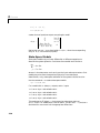
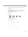
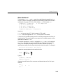
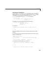
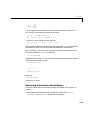
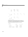
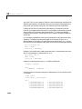
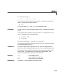
Notice how much the small change in the data is magnified in the solution.
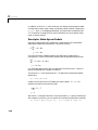
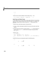
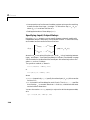
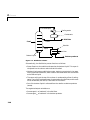
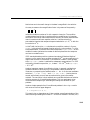
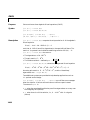
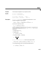
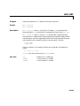
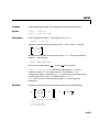
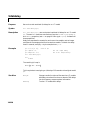
One way to measure the magnification factor is by means of the quantity
A
A
–1
called the condition number of A with respect to inversion. The condition
number determines the loss in precision due to roundoff errors in Gaussian
elimination and can be used to estimate the accuracy of results obtained from
matrix inversion and linear equation solution. It arises naturally in
–1
perturbation theories that compare the perturbed solution ( A + E ) b with the
–1
true solution A b .
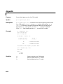
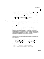
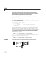
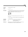
In MATLAB, the function cond calculates the condition number in 2-norm.
cond(A) is the ratio of the largest singular value of A to the smallest. Try it for
the example above. The usual rule is that the exponent log10(cond(A)) on the
condition number indicates the number of decimal places that the computer
can lose to roundoff errors.
IEEE standard double precision numbers have about 16 decimal digits of
accuracy, so if a matrix has a condition number of 1010, you can expect only six
digits to be accurate in the answer. If the condition number is much greater
than 1/sqrt(eps), caution is advised for subsequent computations. For IEEE
arithmetic, the machine precision, eps, is about 2.2 × 10 -16, and 1/sqrt(eps)
= 6.7 × 10 8.
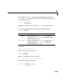
Another important aspect of conditioning is that, in general, residuals are
reliable indicators of accuracy only if the problem is well-conditioned. To
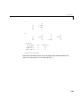
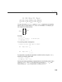
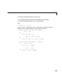
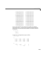
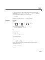
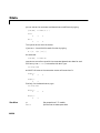
illustrate, try computing the residual vector r = Ax – b for the two candidate
solutions x = [0.999 –1.001]' and x = [0.341 –0.087]'. Notice that the
second, while clearly a much less accurate solution, gives a far smaller
residual. The conclusion is that residuals are unreliable indicators of relative
solution accuracy for ill-conditioned problems. This is a good reason to be
concerned with computing or estimating accurately the condition of your
problem.
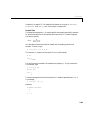
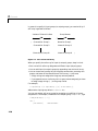
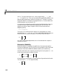
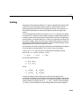
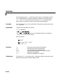
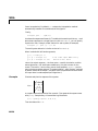
Another simple example of an ill-conditioned problem is the n -by- n matrix
with ones on the first upper-diagonal.
A = diag(ones(1,n–1),1);
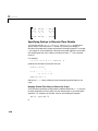
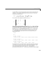
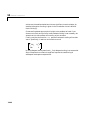
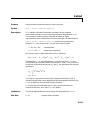
This matrix has n eigenvalues at 0. Now consider a small perturbation of the
–n
data consisting of adding the number 2 to the first element in the last ( n th)
11-5