1
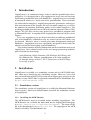
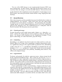
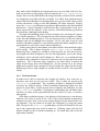
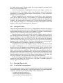
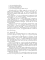
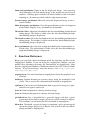
AngioQuant
Antti Niemistö
[email protected]
v1.33 August 11, 2005
Contents
1 Introduction
2
2 Installation
2.1 Standalone version . . . . . . . . . . . . .
2.1.1 Installing the MCR libraries . . . .
2.1.2 Installing AngioQuant . . . . . . .
2.1.3 Starting up . . . . . . . . . . . . . .
2.2 MATLAB toolbox version . . . . . . . . .
2.2.1 Installing the AngioQuant Toolbox
2.2.2 Starting up . . . . . . . . . . . . . .
.
.
.
.
.
.
.
.
.
.
.
.
.
.
.
.
.
.
.
.
.
.
.
.
.
.
.
.
.
.
.
.
.
.
.
.
.
.
.
.
.
.
.
.
.
.
.
.
.
.
.
.
.
.
.
.
.
.
.
.
.
.
.
.
.
.
.
.
.
.
.
.
.
.
.
.
.
.
.
.
.
.
.
.
2
2
2
3
3
4
4
4
3 Usage
3.1 Image quality requirements . . . . . .
3.2 Quantification . . . . . . . . . . . . . .
3.2.1 Opening an image . . . . . . .
3.2.2 Smoothing . . . . . . . . . . . .
3.2.3 Segmentation . . . . . . . . . .
3.2.4 Skeletonization . . . . . . . . .
3.2.5 Pruning . . . . . . . . . . . . .
3.2.6 Single step quantification . . .
3.2.7 Saving the results . . . . . . . .
3.3 Batch processing . . . . . . . . . . . . .
3.3.1 Preparing and starting a batch
3.3.2 Parameter selection . . . . . . .
3.3.3 Saving the results . . . . . . . .
3.4 Viewing the results . . . . . . . . . . .
3.4.1 Visualization in AngioQuant .
3.4.2 Reading CSV files . . . . . . . .
.
.
.
.
.
.
.
.
.
.
.
.
.
.
.
.
.
.
.
.
.
.
.
.
.
.
.
.
.
.
.
.
.
.
.
.
.
.
.
.
.
.
.
.
.
.
.
.
.
.
.
.
.
.
.
.
.
.
.
.
.
.
.
.
.
.
.
.
.
.
.
.
.
.
.
.
.
.
.
.
.
.
.
.
.
.
.
.
.
.
.
.
.
.
.
.
.
.
.
.
.
.
.
.
.
.
.
.
.
.
.
.
.
.
.
.
.
.
.
.
.
.
.
.
.
.
.
.
.
.
.
.
.
.
.
.
.
.
.
.
.
.
.
.
.
.
.
.
.
.
.
.
.
.
.
.
.
.
.
.
.
.
.
.
.
.
.
.
.
.
.
.
.
.
.
.
4
. 4
. 5
. 5
. 5
. 5
. 6
. 7
. 7
. 7
. 8
. 8
. 8
. 9
. 9
. 9
. 10
.
.
.
.
.
.
.
.
.
.
.
.
.
.
.
.
.
.
.
.
.
.
.
.
.
.
.
.
.
.
.
.
4 Option Reference
11
4.1 Menu items . . . . . . . . . . . . . . . . . . . . . . . . . . . . . 11
4.2 Other items . . . . . . . . . . . . . . . . . . . . . . . . . . . . . 12
5 Function Reference
13
1
1 Introduction
AngioQuant is an automated image analysis tool for quantification of angiogenesis. It is designed for in vitro angiogenesis assays that are based on
co-culturing endothelial cells with fibroblasts. AngioQuant uses networks
of connected tubules as a basic unit in the quantification. These networks
are called tubule complexes. AngioQuant provides quantitative and repeatable measurements of the lengths and sizes of tubule complexes as well as
the numbers of junctions (branching points) in the tubule complexes. The
resulting quantification data are saved in the comma separated values (CSV)
format. The CSV files can be easily opened in a spreadsheet program such
as Microsoft Excel®. A snapshot of the AngioQuant software can be seen in
Figure 1.
In in vitro angiogenesis assays that are based on co-culturing endothelial
cells with fibroblasts, endothelial cells are stained so that the tubules can
be detected. However, there is usually also some background staining of
fibroblasts. AngioQuant has been specifically designed to detect only the
tubules and not the more lightly stained fibroblasts.
This manual contains detailed information on the installation and use of
AngioQuant. For technical details of the used image processing methods,
please consult the manuscript
Antti Niemistö, Valerie Dunmire, Olli Yli-Harja, Wei Zhang, and
Ilya Shmulevich, “Robust quantification of in vitro angiogenesis through image analysis,” IEEE Transactions on Medical Image
Processing, in press.
2 Installation
AngioQuant is available as a standalone version and as a MATLAB® toolbox. Most users should use the standalone version. However, users who
have an installation of MATLAB (version 6.5 or higher) may want to use the
toolbox version. MATLAB is a registered trademark of The MathWorks, Inc.
(http://www.mathworks.com/).
2.1 Standalone version
The standalone version of AngioQuant is available for Microsoft Windows
based systems. Most users should choose to install the standalone version
of AngioQuant.
2.1.1 Installing the MCR libraries
The MCR libraries must be installed before installing AngioQuant. The
MCR libraries are available for download on the AngioQuant homepage
at http://www.cs.tut.fi/sgn/csb/angioquant/. The name of the
file to be downloaded is MCRInstaller.exe. The copyright of the MCR
libraries is held by The MathWorks, Inc.
2
Figure 1: A snapshot of the AngioQuant software.
Installation steps:
1. Create a temporary directory (e.g. on the desktop).
2. Copy the file MCRInstaller.exe into the directory that you created.
3. Run the file MCRInstaller.exe. Four files are extracted into the
temporary directory.
4. One of the extracted files is Setup.exe. Run this file and follow the
instructions.
2.1.2 Installing AngioQuant
The AngioQuant software can be downloaded from the AngioQuant homepage at http://www.cs.tut.fi/sgn/csb/angioquant/. The name
of the file to be downloaded is AngioQuant.zip.
Installation steps:
1. Create an empty directory for AngioQuant.
2. Extract the contents of the zip file AngioQuant.zip into the directory
that you created.
2.1.3 Starting up
AngioQuant is started by double clicking on the file AngioQuant.exe. Before trying to start AngioQuant, make sure that you have installed the MCR
libraries (see Section 2.1.1 of this manual).
3
2.2 MATLAB toolbox version
The MATLAB toolbox version of AngioQuant (AngioQuant Toolbox) requires MATLAB 6.5 (R13) or higher with the Image Processing Toolbox. The
toolbox version can be run on any platform for which MATLAB is available.
The toolbox version is mainly intended for advanced users.
2.2.1 Installing the AngioQuant Toolbox
The AngioQuant Toolbox is installed by extracting the contents of the zip
file AngioQuantToolbox.zip into an empty directory.
2.2.2 Starting up
1. Start MATLAB.
2. Go to the directory in which the AngioQuant Toolbox was installed.
3. Start the m-file angioquant.
3 Usage
All the information in this section applies both for the standalone as well as
the toolbox version of AngioQuant.
3.1 Image quality requirements
To get the best quality results from AngioQuant, you need to make sure that
your images are of high quality. First, the imaging should be done soon after
the angiogenesis experiment is finished in the laboratory. This makes sure
that the staining is strong enough to provide a sufficient contrast between
the tubules and the rest of the image. Second, it is important to make sure
that the whole image area is well in focus to avoid blurring of the tubules.
Finally, it is good to have the whole image evenly illuminated. Even though
in most cases AngioQuant is able to correct uneven illumination, an image
that is evenly illuminated is likely to provide more accurate results than an
unevenly illuminated image.
It is important to realize that if your images are of low quality, you are
unlikely to get satisfactory quantification results. The imaging stage is therefore crucial in making sure that the quantification is accurate.
You also need to make sure that you save your images in a file format
that AngioQuant is able to open. The supported file formats are:
• Windows Bitmap (BMP)
• Tagged Image File Format (TIF, TIFF)
• JPEG Image (JPG, JPEG)
• Compuserve Graphics Interchange Format (GIF)
• PC Paintbrush (PCX)
• Portable Graymap File Format (PGM)
• Portable Network Graphics (PNG)
• Portable Pixmap File Format (PPM)
4
The use of the JPEG images is not recommended, because JPEG uses
lossy compression. In other words, some fine details of the images are always lost when the image is saved in the JPEG format. This may cause the
results obtained with AngioQuant to be sub-optimal. If your images are in
JPEG format, converting to another format before using AngioQuant does
not help.
3.2 Quantification
Please note that many of the quantification steps described in this section are
computationally very intensive. Some of the steps may take from couple
of seconds to several minutes to complete. The processing time depends
strongly on the size of the image being processed as well as the computing
power of the computer used. We recommend to use a computer with an
Intel® Pentium® 2.0 Ghz processor (or equivalent).
3.2.1 Opening an image
To open an image in the single image mode, choose Open from the File
menu. Choose the image that you want to process using the dialog that
opens. The image is then displayed on the AngioQuant window. If you
open a color image, it is converted into a grayscale image.
3.2.2 Smoothing
Smoothing is an optional step that in most cases does not have to be performed. However, in some cases smoothing an original image helps to create a good binary image in the segmentation step (Section 3.2.3). Smoothing
is done using the Smooth pushbutton. Smoothing is controlled by the user
defined Kernel size parameter: a high value results in heavier smoothing. If the size of the kernel is one (default), smoothing does not have any
effect on the original image.
3.2.3 Segmentation
To detect and quantify the tubules, you must create a binary image based
on the original (smoothed) image. This is done by pressing the Segment
pushbutton. It is now important to check that the binary segmentation result, overlaid in red on top of the original image, accurately represents the
tubules. The quality of the eventual results is dependent on the accuracy of
the segmentation result, and segmentation is therefore the most crucial step
of the overall quantification procedure.
If the segmentation result is unsatisfactory, a better result may be obtained by repeating the segmentation step with modified parameters. First
you need to use the popup menu in the top right corner of the AngioQuant
window to display the Low thresholding image. A slider now appears
below the image. Use this slider to make sure that at least a part of each
connected tubule complex is overlaid with the red color while at the same
5
time none of the fibroblast or background areas are overlaid with red. Second you need to use the popup menu to display the High thresholding
image. Now use the slider below the image to make sure that all the tubules
are completely overlaid with the red color. It is likely that simultaneously
some undesired (fibroblast or background) areas get overlaid with red, but
it does not matter as long as low thresholding was done correctly. Finally,
press the Segment pushbutton to perform segmentation with the modified
parameters. Again remember to check that the segmentation result accurately represents the tubules. If the result is still unsatisfactory, go back to
fine-tune low and high thresholding.
The high thresholding process can be thought of as selecting all “potential” tubule complexes. The selection of the actual tubule complexes is done
in the low thresholding process. The overlaid read areas in the low thresholding result can be thought of as markers. That is, the idea is to put a red
mark on all tubule complexes, and all those potential tubule complexes that
got marked are selected as actual tubule complexes.
At this point you can also choose to remove tubules that touch the edges
of the image. This is done using the Remove edge tubules checkbox.
Removing these complexes would be motivated by the fact that measuring lengths of tubule complexes that are not completely seen in the image
introduces a bias towards small complexes. However, we recommend not
to remove these complexes, because it too may cause a bias towards small
complexes. This is because large complexes are more likely to touch the
edges of the image than small complexes. In the extreme case, the image
might only contain large complexes that all touch the edges of the image.
Removing all these large complexes would clearly result in a false quantification.
3.2.4 Skeletonization
In order to be able to measure the lengths of tubules, they must be reduced to arcs that are one pixel in width. This is done by pressing the
Skeletonize pushbutton. The resulting skeleton is displayed overlaid
in red on the original image. Tubule junctions (branching points) are displayed as green dots. If you do not want to display the junctions, use the
Show junctions checkbox. Checking or unchecking this checkbox does
not have an effect on the quantification results; rather, it is just a visualization option.
With high resolution images, the displayed skeleton may seem discontinuous even when it really is not. This is due to the limited resolution of
computer screens, that is, the screen cannot display all the data that the image contains. You can zoom in to check for continuity by using the zoom
tool. First press the Zoom tool pushbutton, and then left-click on the image at the region that you want to zoom in. Clicking again with the left
mouse button results in further zooming in. To zoom out, click with the
right mouse button.
6
3.2.5 Pruning
The skeleton that is obtained in the skeletonization step usually contains
spurious short arcs that split from the main lines and are not consistent with
the tubules of the original image. These spurious arcs are removed using the
Prune pushbutton. It is important to select an appropriate Prune size.
This parameter defines the maximum length of a spurious arc. The default
value is 10, which means that all arcs that have 10 pixels or less are removed.
The prune size should be chosen in such a way that the pruning step results
in a clean skeleton that accurately follows the topology of the tubules.
3.2.6 Single step quantification
The smoothing, segmentation, skeletonization, and pruning steps of Sections 3.2.2 through 3.2.5 can be done as a single step using the Quantify
pushbutton. The Kernel size and Prune size parameters as well as
the status of the Remove edge tubules checkbox have the appropriate
effect on the quantification. Single step quantification is useful if you are
able to rely on the automated selection of the thresholds in the segmentation stage.
Note that single step quantification always performs the quantification
starting from the original image and using automated selection of thresholds. If you have modified the thresholds and then press Quantify, the
modified thresholds are ignored.
3.2.7 Saving the results
At any time, the image displayed on the AngioQuant window can be saved
by choosing Save Image from the File menu. The supported file formats
are:
• Windows Bitmap (BMP)
• Tagged Image File Format (TIF, TIFF)
• JPEG Image (JPG, JPEG)
• Portable Network Graphics (PNG)
• Portable Pixmap File Format (PPM)
Saving images in the JPEG format is not recommended, because JPEG
uses lossy compression. In other words, some fine details of the images are
always lost when the image is saved in the JPEG format.
When the skeleton or the pruned skeleton image is displayed on the
AngioQuant window, the respective lengths and sizes of the tubules as well
as the numbers of junctions (branching points) in the tubules can be saved
in a comma separated values (CSV) file by choosing Save Data from the
File menu. The CSV file can then be opened in a spreadsheet program such
as Microsoft Excel. For information on interpreting the CSV file opened in a
spreadsheet program, see Section 3.4.2.
The default CSV separator is the comma. However, in some systems the
separator must be the semicolon in order for the spreadsheet program to
be able to read the CSV file correctly. If the CSV file does not look okay
when you open it in your spreadsheet program, change the CSV separator
7
by choosing Separator Semicolon from the CSV menu, and save the
CSV file again.
If you are using AngioQuant under the Windows operating system, you
cannot save the image or CSV file over a file that is currently opened in
another application such as Excel.
3.3 Batch processing
3.3.1 Preparing and starting a batch
The batch mode allows you to analyze a large number of images without
the need to open each image separately in AngioQuant. Before starting the
batch, you need to put all the images that you wish to include in the batch
into the same directory on your hard drive. Note that a batch cannot include
images that are located on a CD or other read-only media. The batch is
started by selecting Process Batch from the File menu.
3.3.2 Parameter selection
The user makes a number of parameter selections before AngioQuant starts
analyzing the images. Sometimes it may be difficult to know which choices
you should make. In fact, it is often the case that the single image mode is
used with some representative images in order to find the suitable parameters. The batch mode is then used to process a large number of images at
once.
First, AngioQuant asks if the optimal values for the low and high thresholds (see Section 3.2.3) should be found separately for each image. The alternative option is to use the same thresholds for all images. However, it is
recommended to let AngioQuant find the optimal thresholds for each image
separately, because not only may the illumination differ between the images
in the batch, but under different treatments the intensity of the tubules may
vary as well.
If you chose to use the same low and high thresholds for all the images,
AngioQuant may next ask if the parameters used with last opened image or
the last saved batch should be used. If you answer no to both of these questions, AngioQuant next asks whether the low and high thresholds should
be selected automatically or manually. If you opt for manual selection of
the thresholds, AngioQuant next prompts for them.
AngioQuant then prompts for the kernel size for smoothing of the original image (see Section 3.2.2). The higher the value, the stronger the smoothing is. The default value is 1, which means that no smoothing is done.
AngioQuant also asks whether the tubule complexes that touch the edges
of the image should be removed. Removing these complexes would be motivated by the fact that measuring lengths of tubule complexes that are not
completely seen in the image introduces a bias towards small complexes.
However, we recommend not to remove these complexes, because it too
may cause a bias towards small complexes. This is because large complexes
are more likely to touch the edges of the image than small complexes. In the
extreme case, the image might only contain large complexes that all touch
8
the edges of the image. Removing all these large complexes would clearly
result in a false quantification.
As the last parameter, AngioQuant asks the user to give a prune size
(see Section 3.2.5). The choice of this value should in general be based on
experience in analyzing similar images, but typically a value around the
default 10 pixels is suitable.
Finally, AngioQuant asks whether you would like to give descriptive
codes for the different images. If you choose yes, AngioQuant prompts for
the codes one by one and shows each respective image on the AngioQuant
window. The images will be sorted in the CSV file alphabetically according
to the codes that you give. If you choose not to give descriptive codes, the
images will be sorted according to the filenames.
3.3.3 Saving the results
Once all the parameters have been set, AngioQuant analyzes the images
without any user intervention. Please note that running a batch containing a
large number of images may take several hours. If you have a lot of images,
you may want to consider running the batch overnight.
Once the batch is ready to be saved, a popup window appears with the
text “Batch processed successfully”. Press the OK pushbutton to move on to
the save dialog. Use the save dialog to select the name and location of the
comma separated values (CSV) file. The CSV file will contain the quantification data on all the images in the batch. It can be opened in a spreadsheet
program such as Microsoft Excel. For more information on interpreting the
CSV file opened in a spreadsheet program, see Section 3.4.2.
AngioQuant also saves the original images with the skeleton overlaid
in red in a subdirectory skel in your batch directory. You can use these
images to assess the quality of the obtained results. If the skeleton is not
consistent with the underlying image, the quantification results are not reliable, and the analysis should be done again using modified parameters.
Note that with high resolution images, the displayed skeleton may seem
discontinuous even when it really is not. This is due to the limited resolution of computer screens, that is, the screen cannot display all the data that
the image contains. You should zoom in to check for continuity.
If you are using AngioQuant under the Windows operating system, you
cannot save the images or CSV file over a file that is currently opened in
another application such as Excel.
3.4 Viewing the results
3.4.1 Visualization in AngioQuant
In the single image mode, when the quantification results are ready after the
skeletonization or pruning stage, AngioQuant displays the most important
summary statistics on the main window. These statistics are
• number of tubule complexes,
• total length of tubule complexes,
• mean length of tubule complexes,
9
•
•
•
•
total size of tubule complexes,
mean size of tubule complexes,
total number of junctions, and
mean number of junctions per tubule complex.
The lengths and the sizes of tubule complex are measured in pixels. The
lengths are measured from the skeleton of the tubules, whereas the size is
measured from the segmentation result. The size measurement thus takes
into account the thickness of the tubules, and the sizes are therefore larger
than the lengths.
It is also possible to view the quantification results as histograms of the
tubule lengths, sizes, and numbers of junctions. The histograms are shown
by pressing the Show histograms pushbutton.
It is also possible to zoom in the image displayed on the AngioQuant
window. First press the Zoom tool pushbutton, and then left-click on the
image at the region that you want to zoom in. Clicking again with the left
mouse button results in further zooming in. To zoom out, click with the
right mouse button.
The displayed image can also be viewed in an external window. To do
this, press the External image pushbutton. You can have as many such
external windows as you like. Viewing the images in external windows can
be useful, because then you can display at the same time two or more images that you want to compare. You can also resize these external windows.
Zooming is possible by selecting the appropriate tools from the toolbar of
the external window.
3.4.2 Reading CSV files
As described above, the quantification results are saved in a comma separated values (CSV) file in the single image as well as the batch mode. CSV
files are a standard format for saving data in a text file format. They do
not appear evenly spaced in a text file, but they can be interpreted easily by
third party software. If you have a spreadsheet program such as Microsoft
Excel installed on your system, you can load the CSV files into the spreadsheet. You will be able to save the spreadsheet from Excel in its own internal
format, if required.
A part of a CSV file that was saved in the batch mode of AngioQuant
is shown in Figure 2. Note that the quantification results for each image
take up four columns. CSV files that are saved in the single image mode of
AngioQuant are similar. The only difference is that naturally then the CSV
file contains data for only one image.
The first two lines of the CSV file contain the descriptive codes of the images (if applicable) and the names of the image files. If the descriptive codes
were given, the results for different images of the batch are sorted alphabetically according to the codes. Otherwise, the results are sorted alphabetically
according to the filenames.
The next five lines of the CSV file contain the parameters that were used
to analyze each image. These parameters are the kernel size, the low thresh-
10
Figure 2: A CSV file produced by AngioQuant opened in Microsoft Excel.
old, the high threshold, removal of edge tubules (yes/no), and the prune
size.
The last lines of the CSV file give the raw data, that is, the lengths and
sizes of each tubule complex in each image as well as the number of junctions in each tubule complex. For each image, each of these parameters
(lengths, sizes, junctions) take up one column. The data are sorted in a descending order according to the lengths of the tubule complexes. The data
in each row correspond to the same tubule complex. For example, in the
CSV file of Figure 2, the longest tubule complex in img1.bmp has the length
856.93 pixels, its size is 3611 pixels, and it has 16 junctions.
From the raw data it is possible to derive statistics describing the data.
Such statistics include the number of tubule complexes in the image, the
total and mean lengths and sizes of all tubule complexes in each image
as well as the total number of junctions and the mean number of junctions per tubule complex. These seven statistics are given for each image
in the CSV file above the raw data. The same statistics are displayed on the
AngioQuant window in the single image mode.
4 Option Reference
Below you can find information on all the elements of the AngioQuant
graphical user interface. This section serves as a quick reference for users
that are already familiar with AngioQuant.
4.1 Menu items
File Open the File menu.
Open Open an image to be processed in the single image mode (see
Section 3.2.1).
Save Image Save the currently displayed image on the disk (see Section 3.2.7).
Save Data Save the quantification data related to the currently displayed image (see Section 3.2.7).
11
Process Batch Quantify a batch of images (see Section 3.3).
Exit Exit AngioQuant.
CSV Open the CSV menu.
Separator Comma Select the comma as the separator in the CSV files
saved by AngioQuant.
Separator Semicolon Select the semicolon as the separator in the CSV
files saved by AngioQuant.
Help Open the Help menu.
About Display general information on AngioQuant.
4.2 Other items
Select image popup menu Select the displayed image. As you proceed with
the quantification steps, more images corresponding to the different
steps become available in the popup menu. You can use the popup
menu to go back to an earlier step of the quantification process.
Smooth pushbutton Smooth the original image (see Section 3.2.2). The
pushbutton is enabled when the original image is displayed.
Kernel size textbox Select the size of the kernel to be used in smoothing the
image. The higher the value, the heavier the smoothing.
Segment pushbutton Segment the image to recognize the tubule areas (see
Section 3.2.3). The pushbutton is enabled when the original, smoothed,
low thresholding, or high thresholding image is displayed.
Remove edge tubules checkbox Select whether the tubules that touch the
edges of the image are included in the quantification or not. For recommendations, see Section 3.2.3. The checkbox is disabled when the
skeleton or the pruned skeleton is displayed.
Skeletonize pushbutton Skeletonize the segmented image (see Section 3.2.4).
The pushbutton is enabled when the segmentation image is displayed.
Show junctions checkbox Select whether the junctions of the tubules are
shown as green squares on the skeleton. The checkbox is enabled
when the skeleton or the pruned skeleton is displayed.
Prune pushbutton Prune the skeleton (see Section 3.2.5). The pushbutton
is enabled when the (unpruned) skeleton is displayed.
Prune size textbox Select the maximum size (in pixels) of tubules to be removed in the pruning step.
Quantify pushbutton Perform all the quantification steps as a single step
(see Section 3.2.6).
12
Zoom tool pushbutton Zoom in on the displayed image. After pressing
the pushbutton, left-click on the image at the region that you want to
zoom in. Clicking again with the left mouse button results in further
zooming in. To zoom out, click with the right mouse button.
External image pushbutton Show the currently displayed image in an external window.
Show histograms pushbutton View the quantification results as histograms
of the tubule lengths, sizes, and numbers of junctions.
Threshold slider Adjust the threshold in the low thresholding or high thresholding image. The slider is visible when the low thresholding or high
thresholding image is displayed.
Threshold textbox Select the threshold in the low thresholding or high thresholding image. The textbox is visible when the low thresholding or high
thresholding image is displayed.
Reset pushbutton Reset the low or high threshold to the automatically selected value. The pushbutton is visible when the low thresholding or
high thresholding image is displayed.
5 Function Reference
Below you can find a brief description of all the functions (m-files) of the
AngioQuant Toolbox. If you are using the AngioQuant Toolbox, you can
modify these functions to change the functionality of AngioQuant. Note
that the AngioQuant Toolbox is distributed under the GNU General Public
License. If you do not know what this means, visit http://www.gnu.
org/copyleft/gpl.html.
angioquant.m The main function of AngioQuant. Starts the graphical user
interface.
bwthin.m Perform thinning on a binary image using the method by Guo
(1992). This is used as the skeletonization method in AngioQuant.
eqillum.m Correct uneven illumination from a grayscale image by a polynomial least squares surface fit.
fends.m Find end points in a binary skeleton image.
fjunc.m Find junction points in a binary skeleton image.
givehthresh.m Give a threshold for a grayscale image such that a given
percentage of the darker unique graylevels will be marked as objects.
This function is used to find the low threshold in AngioQuant.
hthtesh.m Threshold a grayscale image by marking a given percentage of
the darker unique graylevels as objects. This is used as the low thresholding method in AngioQuant.
13
hystthresh.m Apply hysteresis thresholding for segmentation of an image.
This function is not used in AngioQuant. It may be used to replace
segmcombine.m.
othresh.m Threshold a grayscale image using the method by Otsu (1979).
This is used as the high thresholding method in AngioQuant.
rmbranch.m Remove short branches and small objects from a skeleton image. This is used as the pruning method in AngioQuant.
rmedge.m Remove objects that touch the boundaries of a binary image.
segmcombine.m Apply a variation of hysteresis thresholding for segmentation of an image. This is used as the segmentation method in AngioQuant.
skellen.m Calculate the length of a skeleton taking into account that the
distance between two diagonally connected pixels is not 1 but square
root of 2.
superimpimg.m Create superimposed image from a grayscale image and
red, green and blue masks. This function is used for visualization in
AngioQuant.
thresh.m Threshold a grayscale image using a given threshold.
14