1
JOINTEM
Joint interpretation of electromagnetic and geoelectrical soundings using 1-D layered earth model
User's guide to version 1.4
Markku Pirttijärvi
2010
University of Oulu
Department of Physics
Contents
1.
Introduction
3
2.
Program setup
6
3.
Getting started
7
4.
Menu items
10
4.1
IP settings
13
4.2
Data options
15
4.3
Other options
16
5.
6.
7.
8.
9.
User interface controls
18
5.1
Left control panel
18
5.2
Bottom control panel
23
Data weights
25
6.1
25
Weight editing
File formats
27
7.1
VES data
27
7.2
Duplicate AB/2 values
29
7.3
TEM data
30
7.4
AMT data
33
7.5
Generic data files
34
7.6
Model files
35
7.7
Result files
36
7.8
Graph parameters
36
Additional information
39
8.1
Terms of use and disclaimer
40
8.2
Contact information
40
References
41
Appendix A: TEM graph
43
Appendix B: AMT/VLF-R graph
44
Appendix C: DC/VES graph
45
Appendix D: Weight editing
46
Appendix E: IP effect in TEM inversion
47
Appendix F: SVD graphs
48
2
1. Introduction
JOINTEM is geophysical modelling and interpretation software for:
a) geoelectrical direct current (DC) soundings, a.k.a. vertical electric soundings (VES),
b) time-domain electromagnetic (TEM) soundings (single and central loop),
c) audiomagnetotelluric (AMT) soundings based on plane wave impedance, and
d) frequency-domain VLF-R measurements (single frequency).
The computation is based on one-dimensional (1-D) horizontally layered earth model. The model
parameters are the electrical resistivity and thickness (or depth to the top) of the layers. Cole-Cole
model parameters (chargeability, frequency factor, and time constant) can be used in TEM method
to account for (induced) polarization and dispersion effects. Chargeability can be applied to VES
soundings to account for polarization effects. Optimization based on linearized inversion method
with adaptive damping is used to minimize the difference between measured field data and
synthetic data computed for the model. Both individual and joint inversion of DC, TEM, and AMT
data is possible. VLF-R data measured at single frequency can be used as additional constraint. The
basic principles of VES, AMT, VLF-R, and TEM methods are illustrated in Figures 1-4. For more
information, please, consult any text book of applied geophysics (e.g., Milsom, 2003).
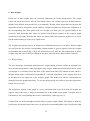
Customary to all geophysical investigation methods, changes in the measured field components, i.e,
static or time-harmonic electric field (or potential) and magnetic field (or magnetic induction) or
changes in the the ratio of two components, are related to changes in the electrical properties of the
earth. This relationship and the characteristic behavior of the geophysical system responses can be
studied with numerical modeling. The aim of geophysical interpretation is to solve the inverse
problem: what kind of a structure could have produced the measurements? To accomplish this, the
difference between the measured data and the modeled data is minimized by parameter
optimization. The result is a simplified model of the real geoelectrical structure that needs to be
interpreted geologically. However, one must remember that the model is only one-dimensional and
the geophysical inverse problem is non-unique. Because real geological structures are complex and
three-dimensional, the results obtained from JOINTEM interpretation may not represent the
geological reality well enough.
3
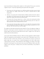
Schlumberger
M
A
N
B
Distance = AB/2
Earth’s surface
Wenner
A
M
N
B
V
a 2
I
Distance = AB = MN = NB
1
1
1
1
rAM rBM rAN rBN
1
Dipole-dipole
A B
M N
Distance = BM
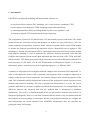
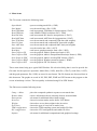
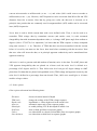
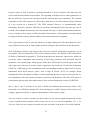
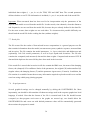
Figure 1. Principle of DC soundings. Current (I) is fed into ground with current electrodes A and B and
electric potential (V), which depends on the electrical resistivity structure of the earth, is measured with
electrodes M and N. The response is defined as the apparent resistivity (a) as a function of electrode
distance (AB/2, AB/3 or BM). With increasing electrode spacing the geometric sounding gives information
from increasing depth. In JOINTEM the three configurations by which the electrodes are positioned are:
Schlumberger, Wenner and dipole-dipole.
Ey
2
1 E x
1 Ey
a
H y
H x
Hy
Hx
Ex
Orthogonal horizontal EM
field components
2
ImE x H y
ImE y H x
arctan
ReE x H y
ReE y H x
arctan
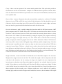
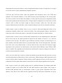
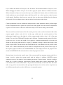
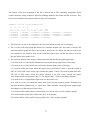
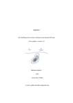
Figure 2. Principle of AMT method. The four orthogonal components of the natural (plane wave) EM field
are measured simultaneously using grounded electrodes (E-field) and induction coils (B-field). After time
series analysis, the processed data are represented as complex impedance, Z = |E|/|H|. Since the earth is
considered one-dimensional the diagonal elements are zero and the off-diagonal elements are the same (Zxy =
Zyx). The AMT response can then be defined as the apparent resistivity and phase. Due to attenuation of the
EM fields the measurements made as a function of frequency (typically between 10 Hz and 10 kHz) give
information as a depth sounding.
4
VLF station
Ez
1 E x
a
H y
Hy
Ex
2
ImE x H y
ReE x H y
Components of the
primary EM field at the
measurement site
arctan
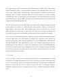
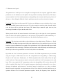
Figure 3. The principle of VLF-R method. Distant VLF antenna (frequency 15-30 kHz) is considered as a
vertical electric dipole. The radial electric field (Ex) and azimuthal magnetic field (Hy) components are
measured and their ratio gives plane wave impedance. As in the AMT method, the response is defined as the
apparent resistivity and phase. Because measurements are made at single frequency, there is minimal
amount of depth information. Therefore, VLF-R data is used only as an additional constraining dataset in the
interpretation.
Current turn-off
I0
Ramp time
loop
x
time
On- time
t1 > t0
Off-time
z
dB0/dt
0
Primary EM pulse
x
time
t2 > t1
t0
z
dBs/dt
Secondary
field decay
x
time
time channels
z
t3 > t2
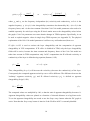
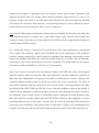
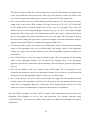
Figure 4. Principle of TEM method. Transmitter loop is laid on the surface of the earth. The (dc) current is
turned off (within few microseconds) thus generating an EM pulse, which generates diffusing "smoke-ring"
currents in the earth. The decaying secondary field of these currents is measured as the voltage (VdB/dt)
induced to the receiver loop or coil during the off-time. The decay rate of the secondary field depends on the
resistivity of the earth. When considering layered earth, the measurements made as a function of time
(typically between 10 s and 10 ms) give information as a depth sounding.
5
2. Program setup
The JOINTEM program is a 32-bit application that can be run on Windows XP/Vista/7 with a
graphics display with a resolution of at least than 12801024 pixels. Memory requirements and
processor speed are not critical, since large data sets are not used and the computations, which are
based on a convolution algorithms and direct analytical solutions for layered earth models, allow
fast computations even on older computers. JOINTEM has simple graphical user interface (GUI)
that can be used to change the parameter values, to handle file input and output, and to visualize the
data and the model responses and the model. The GUI and graphics are based on the DISLIN
graphics library (http://www.dislin.de).
To install JOINTEM simply unzip (Pkzip/Winzip) the distribution file (JOINTEM.ZIP) into a new
folder. You can also create a shortcut on the desktop but in this case you should take care that the
start in folder is the same as the program folder. Otherwise, some extra files will appear on the
desktop too. The distribution file contains the 32-bit executable (JOINTEM.EXE), a short
description file (_README.TXT), user's manual (JOINTEM_MANU.PDF), and some example
data and model files (*_DC.DAT, *_TEM.DAT, *_AMT.DAT & *_.INP).
6
3. Getting started
On startup JOINTEM reads the model parameters from the JOINTEM.INP file and the graphics
parameters from the JOINTEM.DIS file that are located in the program folder. If these files cannot
be found when the program starts, new files with default parameter values are created
automatically. If the format of these files should have become invalid the program halts and a
possible explanation for the error condition can be seen in JOINTEM.ERR file. The program then
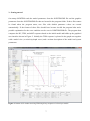
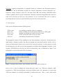
computes the DC, TEM, and AMT responses based on the initial model and builds up the graphical
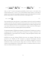
user interface shown in Figure 5. Initially the TEM response is plotted in the graph area together
with a model view (a resistivity-depth curve) and a written description of the model and system
parameters.
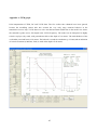
Figure 5. Jointem GUI window showing TEM single loop response of a four layer model.
7
The parameters controlling the modelling, inversion and graphics can be changed using the menu
items and the various controls (widgets) in the main GUI window of the program.
When performing forward modelling the most important functions are:
a) swap between TEM, DC and AMT methods using corresponding push Plot buttons,
b) view alternative response components (TEM apparent resistivity, AMT phase, and DC
apparent chargeability) using Swap comp. button,
c) edit computational parameters such as the minimum and maximum values of TEM time
channels, VES electrode distances and AMT frequencies and TEM source parameter by
editing the text widgets in the left control panel and use Update button to validate changes,
d) set the number of layers and edit model parameters below the graph, or apply Default button
to generate automatically two and three layer models,
e) change TEM system (single or central loop) using Edit/TEM configuration menu, edit source
(receiver) parameters using related fields in left control (Edit/Define receiver item),
f) change VES configuration (Schlumberger, Wenner or dipole-dipole) using Edit/DC
configuration item (for dipole-dipole system define also the dipole length),
g) use Auto axes button to quickly adjust the axis limit of the current graph (and model view).
In the interpretation of measured field data the most important functions (in addition to those
mentioned above) are:
a) import TEM, DC, and/or AMT data using the Read data menu items,
b) set the number of layers in Layers field (and use Update button),
c) create an initial model with Default button,
d) edit model parameters and their fix/free status manually to create better initial model,
e) edit data weights and ignore erroneous data using the Edit weights button,
f) perform numerical inversion using Optimize button.
The optimization is based on linearized inversion scheme where singular values decomposition
(SVD) and adaptive damping are used. Based on an initial model (pk) the inversion iteratively
computes parameter change vector dp from matrix equation Adp= e, where e=d-y is the error
8
vector between measured (d) and computed data (y), and A is the sensitivity matrix (Jacobian) of
dimension NM, where N is the number of free model parameters (columns) and M is the number
of data values (rows). The elements of the Jacobian aij= dyj/dpi are computed numerically as
forward differences. The SVD is defined as A = UVT, where is a diagonal matrix (NN) that
contains the singular values i, V is a NN matrix that contains parameter eigenvectors and U is an
NM matrix that contains parameter eigenvectors. Since U and V are orthogonal the (pseudo)
inverse of the Jacobian is A-1 = VUT and the inverse solution is dp = VUTe, which yields the
updated parameter vector pk+1= pk +dp.
The visual fit between the measured data and computed response, the RMS error, the mean of the
damping factors and the SVD information (singular values and parameter and data eigenvectors)
are used to assess the validity and accuracy of the inversion. Optimally, the RMS error should as
small as possible and the sum of damping factors should be equal to one. However, data weighting
affects the inversion and therefore visual analysis and weight editing play important role also. Note
that the resistivity-depth curve of the model view can (optionally) show the estimated error limits.
The error bars are equal to the 95% confidence limits, which are computed using the information of
the singular value decomposition. Please, refer to Press et al. (1988) for detailed information how
the SVD and confidence limits are computed.
JOINTEM is not an "idiot-proof" interpretation program. It requires a good initial model with a
predefined number of layers. Depending on the initial model the inversion finds a model, which
may be a local minimum of the objective function (data misfit). Therefore, the user should pay
attention to the physical meaning of the results. Special care must be used when interpreting
conductive layers, since due to the equivalence the optimization tends to yield solutions where the
layer conductance (conductivity-thickness product) remains the same but the individual
conductivity and thickness values may vary. Moreover, one should try to keep the models as simple
as possible and avoid using unnecessary layers unless additional a priori information exists. If
depth values are known from seismic interpretations, for example, one should fix the depth of those
layers that are known and optimize layer depth instead of layer thickness. This effectively reduces
the non-uniqueness of the inverse solution.
9
4. Menu items
The File menu contains the following items:
Open Model
Save Model
Read TEM data
Read TEM-fast
Read DC data
Read AMT data
Save TEM data
Save DC data
Save AMT data
Save Results
Read disp.
Save Graph as PS
Save Graph as EPS
Save Graph as PDF
Save Graph as WMF
Save Graph as GIF
open an existing model file (*.INP)
save the model into a file (*.INP)
read in measured TEM data for interpretation (*.DAT)
read AEMR's TEM-Fast 48 data file (*.TEM)
read in measured DC data for interpretation (*.DAT)
read in measured AMT data for interpretation (*.DAT)
save the measured and computed TEM data (and weights)
save the measured and computed DC data (and weights)
save the measured and computed AMT data (and weights)
save the results into a file (*.OUT)
read in new graph parameters from a file (*.DIS)
save the graph in Adobe's Postscript format (*.PS)
save the graph in Adobe's Encapsulated Postscript format (*.EPS)
save the graph in Adobe's Acrobat PDF format (*.PDF)
save the graph in Windows metafile format (*.WMF)
save the graph in GIF file format (*.GIF).
These menu items bring up a typical MS Windows file selection dialog that is used to provide the
file name for the open/save operation. Model files (*.INP), data files (*.DAT), result files (*.OUT),
and the graph parameter file (*.DIS) are stored in text format. The file formats are discussed later in
this document. The graphs are saved in PS, EPS, PDF, WMF and GIF format as they appear on the
screen in landscape A4 size. The best quality is obtained using PS or PDF format.
The Edit menu contains following items:
Comp.->Meas.
Remove Meas.
Data options
Inversion
Weights
Error bars
TEM configuration
DC configuration
Options
place the computed synthetic response as measured data
remove information about (currently shown) measured data
sub-menu for additional data related settings
choose inversion modes and to define VLF-R data
choose how to use data weights in the inversion
choose the type of error bars in model view
choose the TEM sounding system and enable IP effect
choose the VES configuration and enable IP effect
sub-menu for additional computational and graphical settings.
10
Comp.->Meas. sets the response of the current model synthetic data. This option also provides a
fast method to test the inversion and to compare two different model responses with each other.
Note also that menu item Edit/Data options/Add noise can be used to add random (Gaussian) noise
to the synthetic data.
Remove Meas. removes information about the measured data (synthetic or real data). If multiple
datasets exist (e.g, TEM and DC) the user is asked if the information of all data should be removed.
Otherwise only the current data type will be removed. Note that some control widgets and menu
items are inactive (grayed out) before data has been read in for the inversion.
Inversion sub-menu is used to quickly change the inversion mode for full joint inversion, AMT
phase component and VLF-R data. Except for VLF-R data, one can also use the Add to inversion
check box in the left control panel to include (and exclude) the currently shown dataset in (from)
the inversion. VLF-R data is provided manually by setting the frequency (Hz), apparent resistivity
(m), phase (deg.) and weight factor (0,110). The VLF-R data is removed from inversion by
giving an empty line when the program asks for the VLF-R information. When VLF-R data are
active they will be shown in the AMT graph using a different symbol (triangle) shape. Note that
joint inversion is possible only after at least two data sets have been read in and that VLF-R data
cannot be inverted alone. Thickness vs. depth item is used to choose the inversion mode between
layer thicknesses and depth to the top of the layers. These two inversion modes are more or less the
same if thickness or depth values are not fixed. Otherwise they handle a priori data differently. The
current inversion mode is identified in the model information (legend) text.
Weights sub-menu is used to include and exclude the user defined data weights in the inversion.
Weight values range between 0,01 and 100. The smaller the weight is the less importance the data
value has in the inversion. On the contrary, the larger the weight is the more importance the
inversion gives to that data value. Data with weights less than 0,01 are excluded from the inversion
totally. Unit weights are used by default and if the data file did not contain any weights. Weights
can be defined interactively using the Edit weights button described later. Normally weights are not
shown together with the response curve. Separate weight curve can be added to the graph by
selecting Apply and show item in Weights menu. In this case, however, the tick marks of the weight
11
axis on the right side of the graph are shown without labels and axis title to give room for the model
view and information text.
Error bars sub-menu is used to change the appearance of the error bars in model view. The error
bars show the 95% confidence limits (minimum and maximum errors) obtained from the singular
value decomposition used in the linearized inversion method. Note that the confidence limits
depend on the damping factors, which depend on the value of the minimum relative singular value
threshold (Thresh %). Increasing the threshold value imposes stronger damping that produces
narrower confidence limits. Ideally, the confidence limits should be small even if the threshold is
small (no damping at all).
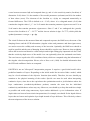
TEM configuration sub-menu is used to define the TEM configuration and the receiver for central
loop system, and to activate the IP effect and Cole-Cole parameters in TEM computations. The
TEM measurement configuration is either: single loop (coincident loop) system, where the source
loop is also the receiver, or b) central loop system, where a smaller receiver loop or coil is located
at the center of the transmitter loop. When central loop system is selected, one needs to define the
radius of the receiver loop b (metres) and the number of loop turns Nr using the Define receiver
item as illustrated in Figure 6. If the Nr is given negative value, b is interpreted as the side length of
a square loop. If Nr is set equal to zero, Rr is considered as the effective area of the loop and the
radius and number loop turns are computed automatically. Note that after measured data have been
read in, the TEM configuration cannot be changed anymore. Also note that in the information text
next to the graph, parameters a and b refer to the side length (and not the radii) of the transmitter
and receiver loops when central loop system is used.
Figure 6. Settings for the receiver in central loop configuration.
12
DC configuration is used to select between a) Schlumberger, b) Wenner and c) dipole-dipole
systems illustrated in Figure 1. Note the different definition of the electrode distance used as the
x-axis in the response graphs. In Schlumberger system the distance is half the current electrode
separation (AB/2). In Wenner system the distance is the equal to the even electrode separation
(AM=MN=NB= AB/3). In dipole-dipole system the distance is the separation between the nearest
current and potential electrode (BM). Note that if measured data has been read in, the electrode
configuration cannot be changed anymore.
The Exit menu has two menu items. The Widescreen item is used to restart the program and build
up the graphical user interface in a mode that suits either normal 4:3 display or widescreen or
laptop displays with greater width. When changing into widescreen mode the user can give
additional value for the aspect ratio. A value between 0,65-0,85 suits most widescreen displays, but
even smaller value should be experimented especially when the screen extends on two displays.
Exit is used to close the program with grace. Emergency exit can be made pressing the close button
in the top right corner of the GUI window or pressing Ctrl-C inside the console window. On
graceful exit the model, results and graph parameters is saved in JOINTEM.INP, JOINTEM.OUT
and JOINTEM.DIS file in the program folder. Copies of the computed (and measured) data are
included in the *.OUT results file. Possible error conditions are reported in JOINTEM.ERR file.
Inside the GUI mode run-time errors are displayed on the screen. Note that result files (and model
files) can be saved at any time using the Save Results (and Save model) menu item. See the chapter
on file formats for more information.
4.1 IP settings
IP effect in TEM is used to activate and deactivate the effect of induced polarization in TEM
computations. By default, IP parameters next to layer resistivities are inactive, which means that
the (dc) layer resistivity is the only electrical model parameter. The polarization and dispersion
effects are described by the Cole-Cole model (Cole & Cole, 1941), in which the frequency
dependent (complex) resistivity or conductivity of the layers is computed using equation (Raiche,
1983)
13
(i ) c
(i ) 0 1
1 (i ) c
or
1 (i ) c
(i ) 0
c
1 1 (i )
,
(1)
where 0 and 0 are the frequency independent (dc) resistivity and conductivity, =2/t is the
angular frequency, (0>>1) is the chargeability (sometimes also denoted by M), c (0>c>2) is the
frequency factor, and is the time constant. Note that Cole-Cole model parameters also need to be
enabled separately for each layer using the IP check marks next to the chargeability values below
the graph. Cole-Cole parameters can create drastic changes in TEM responses. Specifically, it can
be used to explain negative values in single loop TEM response (see Appendix E). The physical
explanation of the Cole-Cole model parameters is still not very well understood, however.
IP effect in DC is used to activate the layer chargeability and the computation of apparent
chargeability in VES computations. If IP effect is disabled in TEM, only the layer chargeability
fields will be active, because the time constant and frequency factor of the Cole-Cole model are
taken into account in TEM computations only. In DC computations the IP affected resistivity or
conductivity of the layer is defined using equation (Sumner, 1959)
'i
i
1 i
or
'i (1 i ) i
(2)
Thus, chargeability (0>>1) will increase the resistivity (decrease the conductivity) of the layer.
Consequently the computed apparent resistivity curve will be different. The difference between the
"ordinary" apparent resistivity (a) and IP affected resistivity (a) is defined as apparent
chargeability (Seigel, 1959)
Ma
a* a
a*
(3)
The computed values are multiplied by 100, so that the unit of apparent chargeability becomes %.
Apparent chargeability values are plotted as a function of electrode distance on a log-linear scale.
To see the apparent chargeability one needs to use the Swap comp. button when the DC graph is
active. Note that the Swap comp. button is inactive if the IP effect in DC is currently disabled.
14
Important: Apparent chargeability is computed mainly for academic and educational purposes.
Different DC and IP instruments measure the induced polarization response differently (e.g.,
integrated voltage, frequency effect FE, and metal factor MF) and currently JOINTEM cannot
compute synthetic data for specific instruments. Therefore, measured chargeability data cannot be
used in the inversion (at least not at the moment). To see if measured data can be scaled to
percentage data one can try to use the Edit/Data options/Norm. data menu item.
4.2 Data options
Data options sub-menu contains following items:
XYZ location
Define title
Reset x-axis
Norm. data
Add noise
set sounding site number and xyz coordinates
define secondary title for the current TEM, DC or AMT graph
multiply current data axis with a user given value
divide current data with a user given value
add random (Gaussian) noise to the data.
The geographic locations of the soundings are not shown anywhere. In practice, measurements are
made along a continuous profile and when put together the interpreted models could be used to
create two-dimensional vertical cross-section of the electrical resistivity. For this purpose it would
be advantageous to be able to use actual geographic coordinates and topographic elevation. At the
moment, JOINTEM does not have this kind of functionality, but as illustrated in Figure 7 the
information is stored in the model files, nonetheless.
Figure 7. Setting the index number, map coordinates, and elevation of the sounding site.
Reset x-axis is used to multiply the current data axis values, e.g, TEM time channels, AMT
frequencies or VES electrode distance, with a user defined value. It is important (!) to know that
TEM time channels are defined and handled in milliseconds (ms). Thus, a value 1000 would
15
convert microseconds to milliseconds (or ms → s) and value 0,001 would convert seconds to
milliseconds (or ms → s). Likewise, AMT frequencies can be converted from kHz to Hz and VES
distances from feet to metres. Note that by giving zero value, the data axis is inverted, so in
principle time periods that are commonly used in magnetotelluric (MT) studies can be converted
into (AMT) frequencies.
Norm. data is used to divide current data with a user defined value. Thus, it can be used to a)
normalize TEM voltage data by transmitter current (and surface area), b) scale measured
chargeability data with instrument dependent value, or c) change AMT phase angle from radians to
degrees (180/= 57,29578). It is important (!) to know that the TEM response is always computed
using unit current (I = 1 A). Therefore, if TEM data have not been normalized with the current
before it is read in, one must use the Norm. data item before continuing with the inversion. Note
that zero value will invert the data, so in principle apparent conductivity can be transformed into
apparent resistivity.
Add noise is used to generate and add random (Gaussian) noise in the data. For AMT phase and
VES apparent chargeability that are plotted on a linear scale the noise level is defined as a
percentage of 45 degrees and 50 %. Thus 100% noise level can give 45 degree change in AMT
phase data. For data that are plotted on logarithmic scale (TEM voltage and apparent resistivity) the
noise level is defined as a percentage from one decade. Thus, 100% error would give to 10 times
smaller or larger values.
4.3 Other options
Other options sub-menu has following items:
Elevation
TEM scale
Depth scale
Auto size
Skin depth
Grid lines
Colors
Line thickness
choose elevation instead of depth
change the scaling of the TEM voltage response
logarithmic vs. linear depth axis in the model view
automatic aspect ratio of the response graphs
to enable plotting VLF-R skin depth in model view
show or hide grid lines in response graphs
use either black or colored (red and blue) lines in response graphs
use either thin or thick lines in response graphs
16
Symbols size
use either larger or smaller symbols in response graphs
By choosing elevation instead of depth one can change the direction of the z axis. Normally z axis
is positive downwards and depth values are computed from the surface or the given z-coordinate of
the sounding site. If elevation is used z-axis is positive upwards and the depth values are computed
with respect to the given z-coordinate of the sounding site, which in turn is usually the topographic
height from the sea level. The use of elevation gives a better possibility to compare models from
surrounding sounding sites and to relate them to the actual topography of the groundwater or
bedrock.
The TEM voltage response is a rapidly decaying curve ranging over several decades (e.g., 10–
10-7 V). Alternative TEM scaling multiplies the TEM voltage data with t5/2, a time dependent factor
equal to the (inverse) time dependency of the late time approximation of the single loop TEM
voltage response. As such the alternative scaling can be considered as "poor man's" apparent
conductivity transform. The alternative scaling is useful when trying to clarify the fit between
measured and computed data, but should not be used when plotting final results. The presence of
alternative scaling is identified by the additional (x t-5/2) at the end of the title of the y-axis.
The remaining items are quite self-explaining. If the depth axis is logarithmic the minimum depth is
computed automatically. If the depth axis is linear the minimum depth is always zero (metres). The
automatic aspect ratio makes the height of the log-log graphs such that a one decade shows up as a
square when the width of the graph is changed using the scroll bar at the bottom of the left control
panel. Alternatively, the aspect ratio can change freely but the height of the graphs is fixed based
on the value defined in the JOINTEM.DIS graph parameter file.
17
5. User interface controls
The various controls of the main GUI window of the JOINTEM program are used for easy access
to the most frequently used settings and actions needed to run the program. The controls on the left
are related to modelling and inversion. The controls below the graph define the model parameters
and their fix/free status in the inversion.
5.1 Left control panel
TEM plot, DC plot and AMT plot buttons are used to change the current response graph between
different sounding methods. If VLF-R data were added in the inversion it can be seen in the AMT
graphs. Depending on the current response graph the horizontal x-axis is either time (milliseconds),
the electrode distance (metres) or frequency (hertz).
Swap comp. button is used a) to change the TEM response graph type between voltage and (latetime) apparent resistivity modes, b) to change AMT response graph between apparent resistivity
and phase data, and c) to change DC response graph between apparent resistivity and apparent
chargeability mode (if the IP effect is enabled for DC computations). If original data were provided
as voltage induced to the receiver loop, it is automatically transformed into apparent resistivity. The
TEM apparent resistivity is computed using the solution defined for the late time voltage response
of single and central loop system above homogeneous half space. However, if the original TEM
data is apparent resistivity it will not be transformed back into voltage data. In this case the Swap
comp. button will be inactive in TEM mode. Likewise, if the AMT data do not include phase
component (so-called scalar AMT measurements) only the apparent resistivity will be used in the
inversion. In this case, however, the Swap comp. button is still active and the modelled phase data
can still be viewed.
Loop, Turns and Ramp define the size (width of the square loop in metres), the number of windings
(integer value), and the length of the ramp time (microseconds) of the TEM transmitter loop. In the
actual computations a square loop is approximated by a circular loop with equal surface area (a2 =
r2). Note that simple linear current ramp is currently utilized, although in most modern
18
instruments the current waveform is a more complicated function of time. If ramp time is set equal
to zero the result is a pure (instantaneous) impulse response.
T/D/F min and T/D/F max define either the minimum and maximum value of the TEM time
channels, VES electrode distances or the AMT frequency range depending on the current graph.
The Points # field is used to define the number of evenly spaced (log-log axis) computation points
between the minimum and maximum values. If dipole-dipole configuration is selected the text field
(Dipole) used to define the dipole length (in metres) becomes visible also. Note that when
measured data has been read in these values cannot be changed, since they are defined in the data.
Update button is used to validate, that is to say, to read in, check and change the values of the
parameters manually edited in the various text fields of the main program window. Note that to
reduce the need for moving the mouse so much the left control panel has two Update buttons.
Default button is used to create an initial model automatically. In the modelling mode (when data
has not been read in) the model parameters depend on the number of layers (2 or 3) and the
resistivity of the top layer. The model is given different resistivity contrasts (10 times larger or 10
times smaller) when the Default button is pressed multiple times. In the inversion mode, when data
have been read in, the default model is derived from the data. Note that VES data has bigger
importance in the creation of an initial model, so the model will be different if only TEM or AMT
data is available. The algorithm used to define the initial model is subject to change in the future so
it will not be described here in detail.
Add to inversion check box is used to exclude and include current data from the inversion or to the
inversion temporarily (without Remove Meas. menu item). When looking at AMT phase data it will
remove only the phase component. When looking at AMT apparent resistivity it will remove both
components, because phase data cannot be used in the inversion without apparent resistivity data.
Data weight is used to give global weight value for individual datasets. By default global data
weights are equal to one so that TEM, DC and AMT data have equal weight. If the weight is
increased that particular data or measurement system is given greater importance than other
datasets. Note that for the AMT data the apparent resistivity and phase components are given
19
separate data weights, so that phase data, for example, can be given smaller importance than
apparent resistivity data. The weight values should preferably range between 0,1 and 10. In
principle, weight value equal to zero will remove that data from the inversion totally (the Jacobian
will contain zero elements). That, however, is not practical because it is more efficient to remove
the data from the inversion using the Add to inversion check box.
Note: If both TEM voltage and apparent resistivity data are available, the inversion will utilize that
data component which is currently active and visible (Swap comp). Because data weights and
scaling are based on the data, the results might be a bit different from voltage based and apparent
resistivity based TEM inversions.
Iters. defines the number of iterations to be performed at a time when optimization is started and
Thres. defines the minimum singular value threshold used in the optimization. This parameter
(which is actually multiplied by 1000) controls the strength of the damping. Decreasing its value
loosens the damping and makes the inversion method work like a steepest descent algorithm.
Increasing its value can be advantageous if inversion is unstable. The default values for the number
of iterations and the threshold are 5 and 0.01 (1.e-5), respectively.
Static shift is used to account for the well known problem with AMT data, where the measured
apparent resistivity values (not the phase data) can be distorted by nearby conductivity variations so
that it has static (independent of frequency) level shift in it. Shift values 10 and 0,1 will move the
measured apparent resistivity data one decade up or down the y-axis, respectively. The effect of
static shift is unknown and can greatly affect the inversion results. Joint interpretation with other
geoelectrical data (VES, TEM and VLF-R) is one of the best methods to improve the quality of
AMT inversion. Although, it could be possible to include the static shift into the joint inversion as a
free parameter, in the current version of JOINTEM it must be adjusted and tested manually. Note
that static shift does not affect phase data and VLF-R data is likely to have negligible or at least
somewhat different level of static shift. Therefore, the fit of VLF-R and AMT phase data can be
used to assess the suitability of the selected value of static shift. If TEM or VES sounding data are
available, the joint inversion can reach good solution only if the value of static shift is properly set.
20
Optimize button is used to perform a predefined number of inverse iterations after data has been
read in and initial model has been defined. The algorithm will adjust all free model parameters so
that the difference between the measured and the modeled data gets minimized. The forward
computation of the VES response of a 1D model is quite fast, so several iterations can be performed
in a few seconds on a modern PC. The TEM response, however, is computationally more
demanding. Therefore, multiple TEM inverse iterations with multiple layers may take few tens of
seconds. After multiple iterations the inversion should converge to a final model and the parameters
cease to change (or they start to oscillate around the final model). At this point the inversion should
be stopped and the accuracy and the validity of the model should be investigated.
Edit weights button is used to enter the interactive weight editing mode. This push button is active
only if data have been read in. Data weights and their editing are discussed later in this document.
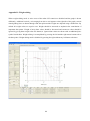
Show SVD button, which is only activate after an inverse iteration, will display a graphical view of
the singular value decomposition (SVD) of the sensitivity matrix, also known as the Jacobian The
SVD plot is illustrated in Appendix F. The first graph shows the parameter eigenvectors, which can
reveal the relative importance and sensitivity of each layer parameter and correlation between
parameters. The second graph, which appears when Show SVD button is pressed again, shows the
data eigenvectors that can reveal the relative importance and sensitivity of each data component
(TEM, DC, AMT) that give the contribution to the corresponding parameter eigenvectors. For more
information about SVD analysis, please, refer to Jupp & Vozoff (1975), for example. When
studying the SVD information it might be worth mentioning that the inversion works with the 10base logarithms of the data and the parameters (resistivity and thickness). The Show SVD option is
experimental and may have been made inactive in the current distribution version of JOINTEM.
Min Y, Max Y, Min X and Max X are used to define the minimum and maximum values of the
horizontal x-axis (TEM time channel, DC electrode distance or AMT frequency) and vertical y-axis
(voltage, apparent resistivity or apparent chargeability) of the response graph.
Auto axes button is used to compute axis limit values for the current graph automatically. In this
case the minimum and maximum values of the axes are set even 10-base logarithms (0.1, 1, 10,
100, etc). If the Auto axes button is pressed twice the axis limits of the model view will be updated.
21
Layers defines the number of the layers in the 1D model. The maximum number of layers is seven.
When changing the number of layers one needs to apply the Update button to validate the action.
When the number of layers is increased new layers are added to the bottom, their text fields become
visible and they are given default values (100 m and 10 m) or their previous values become
visible (again). Similarly, when layers are removed, they are taken away (hidden) from the bottom
of the model. See next chapter how to add and delete layers between other layers.
Update push button is used to validate the changes made to other parameters and to perform single
forward computation and to update the response and model graphs. Note that forward computation
replaces inversion results so that some information may be lost when working with field data.
The two scroll bars at the bottom of the left control panel are used to set the horizontal width of the
response graph (relative value 0,20.6 of the page width) and the vertical position of the
information (legend) text at the right size of the response graph (relative value 00,5 of the page
height). The size of the TEM and DC graphs can be different. If automatic graph sizing (Edit/Other
options/Auto size) is active the height of the graphs is computed automatically so that the one
decade on the log-log graph shows as a square. If automatic resizing is inactive the height of the
graphs is equal to the value defined in the JOINTEM.DIS file. Note that the size and position of the
model view is defined automatically and it cannot be changed and that the position of the origin of
the response graph is defined in the JOINTEM.DIS file. The changes made to the graph size are
stored in JOINTEM.DIS file and used the next time the program is started.
Backup button is used to take a quick copy of the current model into program memory and Revert
button is used to replace the current model with the backup. In addition, JOINTEM creates
automatic copies of the model a) before updating the model (Update button), b) before reading a
model file, c) before creating an initial model (Default button) and d) before optimization. The
Undo button will revert the model back to the previous automatically saved model. Note that Undo
takes a copy of the current model so that pressing the button twice can be used to swap between
two different models and to see their difference on computed response.
22
5.2 Bottom control panel
The parameters of each layer are set using the text widgets below the response graph. The model
parameters are: the thickness (or the depth to the top) and the resistivity (ohm-metres) of the layers
(metres) and the Cole-Cole model parameters (chargeability, time constant and frequency factor) of
the layers. After editing the fields the Update push button must be used to activate the changes.
Useful tip: Single layer can be removed if it is given zero thickness or zero resistivity value. A new
layer can be added between other layers one if it is given negative resistivity value. Actually in this
case, the layer will be split into two layers. The bottom layer cannot be split into two, but
increasing the number of layers has the same effect.
When pressed with the left mouse button the check marks (fix) on the right side of each parameter
field are used to fix and free parameters in the inversion. Fixed parameter will identified by a *
character next to its value in the information text. By default all parameters are free.
Important: The inversion works either on layer thickness or layer depth values (Thickness vs. Depth
menu item). The depth inversion mode allows the depth to the top of a particular layer to be fixed
based on a priori information. For example, if the groundwater level is known then the layer related
to that should be fixed accordingly. Thickness inversion mode works differently and would require
that all layers above the groundwater level are fixed (which is not desirable).
By default the Cole-Cole model parameters are inactive. For TEM computations they are enabled
using the IP effect in TEM menu item. For DC computations the chargeability is enabled using
IP effect in DC menu item. Furthermore, for TEM computations the check marks (IP) at the right
end of each row of layer parameters must be activated to enable the Cole-Cole parameters for each
layer. This is not required in DC computations, where the chargeability will be active whenever IP
effect is enabled. Note that Cole-Cole model parameters should not be activated for every layer,
(because of ambiguity and slowness of inversion). Instead, a single layer (e.g., clays or schists)
should be made responsible for the polarization effects. Even then the inversion should not try to
optimize all three Cole-Cole model parameters together. Instead, the frequency factor should be
23
fixed and tested using a trial-and-error method while the time constant and chargeability can be free
parameters. Please, note that physical interpretation of IP parameters is quite ambiguous.
Because of the high frequency (10-25 kHz) of the VLF-R method, it has quite limited depth of
investigation. The depth of investigation is related to the (plane wave) skin depth defined as:
2
503
f
m
,
(4)
where is the resistivity of the medium (m) and f is the frequency (Hz). To be able to visually
estimate the depth of investigation, the cumulative skin depth at the given VLF-R frequency is
shown as a horizontal dashed line in the model view. The cumulative skin depth is computed by
adding the electric attenuation in each layer until the amplitude reaches 1/e of its original value.
The line can be removed from the graph using corresponding item in Edit/Other options sub-menu.
The remaining four text widgets at the right end of the bottom control panel are related to the model
view. These values are used to change the minimum and maximum value of the horizontal
resistivity axis (in ohm-meters) and the step and maximum value of the vertical depth axis (in
metres). The step value is used only when the depth is plotted using linear scaling. Minimum depth
value is always zero for linear depth axis and some rounded 10-base logarithm value for
logarithmic depth axis. Automatic axis limit values can be set to the model graph by pressing the
Auto axes button twice.
24
6. Data weights
Proper use of data weights plays an extremely important role in the interpretation. The weight
values can vary between 0,01 and 100. The default value is one, which is given to all data values by
default if not defined in the model file or set manually. Weight values larger than one increase the
importance of those data points. On the contrary, weights less than one decrease the importance of
the corresponding data. Data points with zero weight (less than 0,01) are ignored totally in the
inversion. Such discarded data values are plotted with different symbol in the response graph
(marked by a plus-sign). Note that the values are relative and if all weights are equal to 10 or 0,01 it
has the same meaning as if they were equal to one.
The weights represent the inverse of measured or estimated data errors or variances. When weights
are read from the file and the corresponding column number is given a negative value the weights
are automatically inverted (Wg= 1/Wg) and scale between 0,01 and 100. The method used to define
weights from data error is likely to change in the future and will not be discussed here in detail.
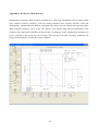
6.1 Weight editing
The user should get accustomed with interactive weight editing, because it plays an important role
in successful interpretation. After pressing the Edit weights button the normal mouse arrow cursor
will change to a crosshair cursor and most of the menu items and GUI controls become inactive.
Weight editing mode is illustrated in Appendix D. A second, logarithmic y-axis ranging from 0,01
to 100 appears to the right side of the response graph. The model view and the information text
disappear from the graph temporarily. To exit the editing mode one needs to press the right mouse
button once (or twice).
The weights are plotted on the graph as a curve with dashed line style. By default, all weights are
equal to one so the curve is simply a horizontal line in the middle of the graph. If weight value is
less than 0,01 the corresponding data value is identified by a plus-sign over it.
Vertical lines are drawn through each data value to guide weight editing. The editing is made by
pressing the left mouse button once above or below the corresponding data value. Pressing the right
25
mouse button finalizes the editing and the weight curve will be updated. This way one can edit the
weights one-by-one. To speed up weight editing some special tricks can be applied:
If one presses the left mouse button at two different positions (and then presses the right
mouse button) the weights between those two points are adjusted based on linear
interpolation.
Likewise, if one presses the left mouse button at different positions from left to right or
from right to left (and then presses the right mouse button) spline interpolation is used to
adjust all the weight values between the outermost points.
If one presses the left mouse button above or below or below the actual graph (and then
presses the right mouse button) the weight of that particular data point is set value 0.01,
which means that it will be excluded from the inversion.
If one presses the left mouse button on the left or on the right side of the graph (and then
presses the right mouse button) all weights, even the previously excluded ones, are set to
that value. This is the easiest way to reset all weights.
The weights are stored both in the data files and in model files. Thus, after editing the weights one
should save the data again so that the interpretation can be restarted afterwards using previously
defined weights. Note that after measured data has been read in, weights are not read from the
model file (just the model parameters).
Also note that VES and TEM data usually have different resolving capabilities at different depths.
Unlike DC method that has good resolution for near surface layers, TEM method is more or less
blind to near surface resistive layers. Therefore, it may not always be necessary to increase the
global weight value. As a matter of fact, it would be advantageous to be able to define relative
weight separately for each layer. This would allow the VES soundings, for example, to have bigger
importance in resolving the near surface and resistive layers and TEM data could be given more
weight to resolve deep layers. Currently, however, this kind of functionality is not provided in
JOINTEM.
26
7. File formats
When using the program for interpretation purposes make sure that your input data files (*.DAT)
are formatted properly. Note also that one can determine the file format from the output of
modelled data (File/Save data). In DC case, however, the measured current and voltage values are
replaced by apparent resistivity. Saved data files also include interactively edited weights.
For each data type (VES, TEM, AMT) two file formats are supported: a) generic column formatted
data file without header information, and b) column formatted data file with header information.
Important: The first line of the file determines how the file will be handled. If the file starts with #,
/, or ! -characters it is considered to be a generic column formatted data file and the user needs to
provide all the necessary header information interactively. Otherwise, lines that start with #, /, or !
-characters are considered comment lines and they will be ignored.
7.1 VES data
The following example illustrates the format of the VES data file with header information:
DC example
# 07.06.2007
# EDA R-PLUS
# 3422126,7179893 YKJ
1
25
2
4
8
8
...
40
40
60
80
100
0
1
0
2
6
7
0.5
0.5
0.5
2
11.8
49.5
200
47.1
733.1
216.8
69.1
261.6
92.7
88.1
100.8
100.9
93.318
121.811
137.103
122.114
1
1
1
1
2
5
5
5
5
1250
495
1120
2002
3133
8.7
22.7
7.69
2.8
1.43
87.2
87.1
103.1
89
83.2
124.713
129.006
83.538
62.984
53.848
1
1
1
1
1
The next relevant line "1 0 0" has three integer values that define: a) measurement array (IMOD),
b) data type (IDAT), and c) IP related chargeability option (IMOC).
27
Measurement array is either: Schlumberger (IMOD= 1), Wenner (IMOD= 2), or dipole-dipole
(IMOD= 3). Data type is either: apparent resistivity (IDAT= 0) or current and voltage (IDAT= 1).
The IP effect is either disabled (IMOC= 0) or disabled (IMOD= 1) in DC computations.
The next line defines the number of data values (NOA), column number of the current electrode
AB distances (ICOA), column number of the potential electrode MN distances (ICOM). Depending
on the value of data type the line also defines a) if IDAT= 0 the column indices of the apparent
resistivity and its weight, or b) if IDAT= 1 the column indices of current, voltage, and weights.
In the example, IDAT= 0 and apparent resistivity will be read from the sixth column. If the first
line were "1 1 0" (IDAT= 1), the second line could be "25 1 2 3 4 7" and current and voltage
values would be read from columns 3 and 4. Note that for Wenner data, there is no need to define
the column for potential electrodes, so it can be is ignored (e.g. "25 1 0 6 7"). Likewise, weights
will be ignored if its column number is equal to zero (e.g. "25 1 2 6 0"). Moreover, if weight
column is given negative value (e.g., "25 1 2 6 -7") weights are considered as data error, that
means they are inverted and scaled between 1 and 0,01.
If IP effect is enabled in DC computations (IMOC=1), then two additional parameters that define
the column numbers of the measured apparent chargeability data and its weight must be given at
the end of the second line. In the current version of JOINTEM chargeability data are not used in
inversion and therefore the chargeability weights are always ignored (e.g. "25 1 2 6 7 8 0").
The remaining lines define (in column format) the electrode distances, the DC sounding data and
(optionally) the data weights. For Schlumberger array the first column defines AB/2 distances (see
Figure 1 for explanation) and the second column the MN/2 distances. For Wenner system the first
column defines AM= MN= NB distances and the second column is not needed, because voltage
electrodes are placed evenly between the current electrodes. For dipole-dipole system the first
column is the BM distance and the second column defines the dipole length (a=AB=MN), which is
usually constant. Electrode distances are given in metres (m), the apparent resistivity in ohm-meters
(m), the current in milliamperes (mA), and the voltage in millivolts (mV). Since the ratio of
voltage and current is used to compute the apparent resistivity, the unit of current and voltage data
can be amperes and volts as well (but never amperes and millivolts).
28
If current and voltage values are read from the file they are replaced with apparent resistivity that is
computed using the equation for homogeneous half space:
V
a 2
I
1
1
1
1
rAM rBM rAN rBN
1
,
(5)
where V is the measured potential difference between electrodes M and N, I is the current fed into
electrodes A and B (positive and negative) and rij are the distances between the four electrodes.
The maximum amount of VES data (AB/2 values) is 80 data points. The header text is used as a
secondary title in the response graphs. If the header text is empty the default title in the
JOINTEM.DIS file is used instead (can be left empty). Apparent resistivity (current and voltage)
values equal to zero are ignored.
7.2 Duplicate AB/2 values
The electric potential created by a grounded electrode (point source of current) on a homogeneous
half space is a proportional to the inverse of the distance (e.g., 1/rAM). As the electrode spacing
AB/2 increases the potential decreases and it is therefore necessary in Schlumberger configuration
to increase the potential electrode distance (MN/2) every now and then. Otherwise the potential
difference becomes so small that it cannot be measured accurately anymore.
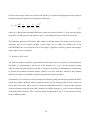
Unfortunately, the earth is not really homogeneous and the voltage measured using different MN/2
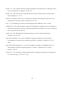
values may produce different value of apparent resistivity. This unknown shift can be corrected if
two or three successive AB/2 values are measured using different MN/2 values and the apparent
resistivity obtained with the larger MN/2 distance are shifted along the a axis to fit those obtained
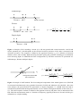
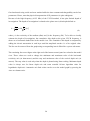
with smaller MN/2 distance. The correction, which is illustrated in Fig. 5, is also discussed in the
book of Milsom (2003).
29
log a
curve 1
curve 2
curve 3
shift 1
Corrected curve
shift 2
log AB/2
Figure 8. The method used to correct shifted apparent resistivity data measured with overlapping
AB/2 values when potential MN/2 distance is increased in the Schlumberger configuration.
When JOINTEM reads in VES data it automatically searches for data made with same AB/2 and
different MN/2 values. Based on the mean of the differences in the apparent resistivity (on a
logarithmic scale) the a values measured with the larger MN/2 spacing are then adjusted
accordingly. Note that shift correction may not be successful if any of the duplicate soundings are
erroneous. Typically the errors arise from the fact that MN distance has not been increased in time
when field measurements were made (small voltage values gives large relative errors). Therefore,
one should analyze the response graphs for multiple MN/2 values, preferably with and without the
shift correction (may be implemented in future version of JOINTEM).
7.3
TEM data
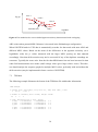
The following example illustrates the format of the TEM data file with header information:
TEM example
# single loop: volts/amps, loop size (m), ramp time (mms), turns
0
50.00
5.000 1
# number of channels, data column, weight column
36
1
2
4
# time, measured volts & rhoa, weight
0.0041
0.4743000E-01
0.1558684E+04
0.0051
0.6219999E+00
0.1948152E+03
0.0061
0.4837000E+00
0.1709358E+03
...
1.6561
0.2733000E-05
0.4733648E+02
1.9131
0.1899000E-05
0.4744464E+02
1.0
1.0
1.0
1.0
1.0
30
The first relevant line defines a) the TEM measurement system and data type (IMOT), b) the side
length of the square transmitter loop (metres), c) the duration of the ramp-like current turn-off
(microseconds), and d) the number of loop windings of the transmitter loop (integer value).
The measurement system IMOT = 0, 1 or 2 for single loop system and IMOT= 4 or 4 for central
loop system. The data type IMOT= 0, 1 or 3 for voltage response (normalized with current) and
IMOT= 2 or 4 for apparent resistivity response.
In central loop system two additional parameters that define: 5) side length of the square receiver
loop (metres) and number of loop windings of the receiver loop are needed (e.g., "0
5.0 1 0.5 100".
50.0
If the number of loop windings is negative, then the side length of the transmitter
and/or receiver loop is interpreted as the radius of the loop. If the number of loop windings is equal
to zero, the side length is interpreted as the area of the loop and the size of the transmitter and/or
receiver loop is computed automatically.
The next line defines the number of data values (NOT) and the column numbers of the time
channel, the TEM data and weights. Weights are not read if its column number is zero. Moreover,
if the weight is given negative column number (e.g., "36
1 2 -4")
the weights are inverted and
handled like data error.
The remaining NOT lines contain the time channels (center of the time windows in ms), the
normalized voltage (V/A) or the apparent resistivity values (m), and (optionally) the data weights
in column format. Time values should be given in milliseconds but they can be adjusted (e.g., s
ms) using Edit/Data options/Reset x-axis menu item. Likewise, TEM data that have not been
normalized with transmitter current can be adjusted using Edit/Data options/Norm. data item.
If data are provided as voltage induced into the receiver, it will be transformed into apparent
resistivity automatically. The apparent resistivity is computed using the late time approximation for
a large loop on the surface of homogeneous half space at. The apparent resistivity of single loop
and central loop TEM systems are (Spies & Frischknecht, 1991):
31
1
2
0 5 a 8 3 a 4 3 0 5 / 3
and
a (t )
5 2
20
S
t
400 t S
2
a 2 nb 2 3 0
a (t )
20
S
t
5/3
,
(6)
where 0= 410-7 Vs/(Am) is the magnetic permeability of the free space, a is the radius of the
circular transmitter loop, t is time, S= v(t)/I is the normalized voltage response, b is the radius of
circular receiver loop and n is the number of loop turns on the receiver. One should also remember
that the voltage response is related to the time derivative of the magnetic field
v(t ) 0 nb 2
hz
.
t
(7)
Thus, data defined as the time derivative of vertical magnetic field can be rescaled to normalized
voltage data (divided with 0nb2I) using the Edit/Data options/Norm. data item. Please, note that
data read in as apparent resistivity will not be transformed back into voltages and therefore Swap
comp. button will be inactive. Users are recommended to use voltage values for the TEM response,
because the other software may compute apparent resistivity differently.
The maximum amount of TEM data (time channels) is 80 data points. The header text is used as a
secondary title line in the TEM response graph. If the header line is empty the default title in the
JOINTEM.DIS file is used instead (can be left empty). Voltage and apparent resistivity values
equal to zero are ignored.
JOINTEM can also read (File/Read TEM-Fast data item.) text formatted *.TEM data files
generated by the TEM-Fast 48 HPC instrument by Advanced Electromagnetic Research
(http://www.aemr.net). The file format is specific to the TEM-Fast instrument it will not be
described here. Please, note that only the voltage data are read from *.TEM. Also, if the file
contains several soundings they are listed together with the xy-coordinates and the user needs to
choose one of them interactively (see Figure 9).
32
Figure 9. Selecting sounding data from a *.TEM file with multiple soundings.
7.4
AMT data
The following example illustrates the format of the AMT data file with header information:
AMT example
# number of frequencies, freq, rhoa, phase & weight columns
21
1
2
3
4
5
# freq (Hz), rhoa (Ohmm) & phase (deg.), weights
30.00 0.9114084E+03 0.4248446E+02 1.00 1.00
40.00 0.8956744E+03 0.4204181E+02 1.00 1.00
60.00 0.8773687E+03 0.4152812E+02 1.00 1.00
...
20000.00 0.1734963E+03 0.2574255E+02 1.00 1.00
30000.00 0.1449312E+03 0.2679170E+02 1.00 1.00
As the example shows, the first relevant line defines the number of data points (NOF) and the
column numbers of frequency (Hz), apparent resistivity (m), phase angle (degrees) and the
weights of apparent resistivity and phase. If the column number of frequencies is negative the
frequencies are interpreted as time periods (commonly used in magnetotellurics) and inverted
accordingly (f = 1/t). If the column index of the phase data is zero, the phase data can be missing as
in the so-called scalar AMT measurements. Weights are ignored if their column numbers set equal
to zero (e.g., "
21
1
2
3
0
0").
If weights are given negative column number they are
interpreted as data error. This means that the values are inverted because the smaller the data error
is the larger should the weight be. Since the weights must vary between 100 and 0,01 the inverted
data error values are further normalized between 0,01 and 1.
33
The maximum amount of AMT data (frequencies) is 80 data points. The header text is used as a
secondary tile line in the AMT response graph. If the header line is empty the default title in the
JOINTEM.DIS file is used instead (can be left empty). Apparent resistivity and phase values equal
to zero are ignored.
7.5
Generic data files
If the first line starts with a comment ( #, / or !) character, the file is considered to be in generic
column format without any header information.
The example below illustrates the format of the generic data file in case of AMT method:
# AMT freq, rhoa, phase, rhoa wei, phase wei
30.000 0.9114084E+03 0.4248446E+02
1.0
1.0
42.376 0.8956744E+03 0.4204181E+02
1.0
1.0
59.858 0.8773687E+03 0.4152812E+02
1.0
1.0
...
Depending on the sounding method (TEM, VES, AMT) the user must provide all the relevant
information about measurement system, data type and the column order interactively using the
dialogs that will appear on the screen. Most importantly, the user needs to provide correct column
numbers for the system variable (time, distance, frequency), data and weights. The header line is
shown to the user, and therefore it would be advantageous if it shows the column information as in
the example. For example, to read the AMT data above one could provide column information as
"1 2 3 4 5" or "1 2 0 4 0", if phase data is not available or needed (see Figure 10). Note that the
number of data values (time channels, distances or frequencies) is not needed and the sign of the
weight column is handled as with normal data files with header information. Reading generic TEM
data is a special case, since the user is asked to provide transmitter current (A) and a time scale
value so that the data can be converted accordingly (V/A and ms). If the data is needed again it
should be saved using the Save data menu item to avoid the cumbersome interactive reading.
34
7.6 Model files
The format of model files is not discussed here in detail because they do not need to be edited. The
following example shows only the top of the file, where the model is defined.
* JOINTEM v. 1.31 model file:
station n:o, xyz-coordinates (m)
0
-175
0
200.0
layer total number
4
thi (m), rho(ohmm), charg, tau, freq (fixes
0.340E+01 1 0.163E+06 1 0.10E+00 1 0.10E+01
0.460E+02 1 0.226E+03 1 0.10E+00 1 0.10E+01
0.112E+03 1 0.259E+02 1 0.10E+00 1 0.10E+01
0.000E+00 0 0.100E+04 0 0.10E+00 1 0.10E+01
between), IP
1 0.10E+00 1
1 0.10E+00 1
1 0.10E+00 1
1 0.10E+00 1
on/off, depth, elev
0 0.000E+00 0.200E+03
0 0.340E+01 0.196E+03
0 0.494E+02 0.150E+03
0 0.162E+03 0.375E+02
TEM, DC, AMT modes & weigths + VLF-R option
1
1
0
1
1
0
1
Tx side (m), turns, ramp (µs), Rx side (m), turns
...
The first line defines the file version number, which is essential information. The x and y
coordinates are defined as integers and z coordinate, i.e., the topographic elevation has floating
point (real) value. Fixed parameters are labeled with a zero after them and free parameters are
labeled with 1. The IP on/off parameter (0=no IP, 1= IP used) enables or disables the Cole-Cole
parameters for each layer. Depth and elevation are extra information, since they are computed from
the values of z coordinate and layer thicknesses.
After line the model parameters defines the different sounding methods. The first three parameters
(IMOT, IMOD and IMOA) define TEM, DC and AMT modes. IMOT= 0 for single loop system
and voltage response, IMOT= 1 for single loop system and apparent resistivity response, IMOT= 2
for central loop and voltage response and IMOT= 3 for central loop and apparent resistivity
response. IMOD= 1 for Schlumberger, IMOD= 2 for Wenner, and IMOD= 3 for dipole-dipole
system. Negative value (IMOD < 0) informs that IP chargeability is enabled for DC computations.
IMOA= 0 if phase component is used in inversion and IMOA= 1 if the phase information is not
going to be used. The next three parameters define whether or not the model file also contains
35
individual data weights (1 = yes, 0= no) for TEM, VES and AMT data. The seventh parameter
defines whether or not VLF-R information is included (1= yes, 0= no) at the end of the model file.
Important: When measured data has been read in for interpretation only the parameters of the
layered earth model are read from the model file. In other words, time channels, electrode distances
and frequencies are not read from the model file, because they are already defined in the data file.
For the same reason, data weights are not read either. To circumvent this possible difficulty one
should read the model file before reading the data (without weights).
7.7 Result files
The file created for the results of forward and inverse computations is a general purpose text file
that contains information about the model, measurement system, synthetic response, measured data
and inversion. The file contains the model parameters, i.e., layer resistivities and thicknesses and
(optionally) Cole-Cole model parameters, as well as layer depths and elevations. The file also
contains the computed (and measured) data and the data weights. Computed and measured VLF-R
data and skin depth are also stored if they have been used in the inversion.
If the result file is stored after inversion it will also contain the RMS error, the mean of the damping
factors, the (damped) 95% confidence limits of the parameters, the original (W) and normalized (S)
singular values, the damping factors (T) and the parameter eigenvectors (V-matrix). In addition, the
file contains in a suitable format the necessary information required to plot the model curve and the
error bars using a third-party plotting program.
7.8
Graph parameters
Several graphical settings can be changed manually by editing the JOINTEM.DIS file. Most
importantly, one should be able translate all character strings used in the response graphs into local
language if needed. Note that the format of the file is essential and if the file should become
corrupted (so that program won't start or the graphs are messed up), one should delete the
JOINTEM.DIS file and a new one with default parameter values will be automatically generated
the next time the program is started.
36
The format of the first paragraph of the file is shown below. The remaining paragraphs define
various character strings related to different sounding methods, the model and the inversion. They
have been omitted because their meaning is quite self-explaining.
JOINTEM v. 1.31 GUI & graph parameter file
40
32
32
26
26
1
1
1
1
0
0
1
0
1
370
330
0.500 0.575 0.575 0.575 0.850 0.000 0.830
0.10000E-02 0.10000E+02 0.10000E+01 0.10000E+07
0.10000E+01 0.10000E+03 0.10000E+03 0.10000E+07
0.10000E+02 0.10000E+06 0.10000E+04 0.10000E+05
0.10000E+02 0.10000E+07 0.10000E+02 0.50000E+02
...
0.10000E+02
0.90000E+02
0.40000E+02
0.10000E+06
0.11000E+03
0.50000E+02
The first line is a title or description for the file itself and the second line is left empty.
The 1.st line of the first paragraph defines five character heights. The first value is used for the
main title and the graph axis titles, the second is used for the axis labels, the third is used for the
plot legend text, the fourth is used for the model description text, and the last value is used for
the axis labels in the model view.
The 2.nd line defines some integer valued parameters that modify the graph appearance:
#1 is used to set (1/0) the model information text to/from the top-right corner of the page.
#2 is used to set (1/0) the model view to/from the bottom-right corner of the page.
# 3 is used to define the corner where the legend text is positioned. Values 1-4 put the legend in
SW, SE, NE or NW corner of the page (outside the graph). Values 5-8 put the legend in the SW,
SE, NE, or NW corner inside the graph. Default is the SW corner outside the graph.
#4 is used to define screen aspect ratio, 0= 3:4 display and 1= wide screen/laptop displays.
#5 is used to set (1/0) logarithmic depth scale for the model view.
#6 is used to set on (1/0) automatic aspect ratio for the log-log response graphs. Normally loglog plots should be plotted using 1:1 aspect ratio. Thus, automatic sizing adjusts the graph height
according to its width and axis limit values
#7 is used to define either black or colored lines (0/1) for the curves in the response graphs.
#8 is used to define either thin or thick line (0/1) in the graphs.
#9 is used ti define either small or large symbols (0/1) in the response graphs.
37
The last two numbers define the x- (horizontal) and y- (vertical) offset distance (in graph pixels)
of the origin from the bottom-left corner of the page. Note that these values are related to the
size of the (landscape A4 sized) page area, which is equal to 29702100 graph pixels.
The 3.rd line defines some real valued (floating point) parameters. The first defines the relative
length of the x axes of the TEM (voltage 0.5 & app. resistivity 0.575), DC (0.575) and AMT
(0.575) graphs and the maximum height (0.85) of the y axis (in all graphs). These values are
relative to the size of the width and height of the plot area (eg. 0.5= 50 % of the width or height)
without the offsets of the origin. The sixth parameter defines the relative vertical position (from
the top of the graph) of the model information text next to the graph. The last parameter defines
the value used to change the aspect ratio of widescreen displays. Note that workstations with two
display screens make DISLIN to compute the horizontal width of the.
The 4.th line defines x and y axis ranges for the TEM graphs. The six parameters are the limiting
values of the logarithmic time axis (in milliseconds), the limiting values of the logarithmic
voltage axis (micro-volts) and the limiting values of the logarithmic apparent resistivity axis
(ohm-meter).
The 5.th line defines x and y axis ranges for the DC graphs. The six parameters are the limiting
values of the logarithmic distance axis (in metres), the limiting values of the logarithmic
apparent resistivity axis (ohm-meter), and the limiting values of the linear apparent chargeability
axis (%).
The 6.th line defines x and y axis ranges for the AMT graphs. The six parameters are the
minimum and maximum value of the logarithmic distance axis (in metres), the minimum and
maximum value of the logarithmic apparent resistivity axis (ohm-meter).
The 7.th line defines x and y axis values for the model view graph. The four parameters are the
limiting values of the logarithmic resistivity axis (ohm-meter), the step and the maximum value
of the linear or logarithmic depth axis (ohm-meter). The minimum depth is always zero if the
depth axis is linear and automatically computed if the depth axis is logarithmic.
Note that DISLIN graphics uses ISO Latin-1 character codes and control characters that allow
displaying Greek alphabets as well as sub- and superscripts. For example, character string
"({M2}W{M1}m) " will create text "(m)" in the graphs. See DISLIN documentation for further
information.
38
8. Additional information
The JOINTEM program is based on DCINV program for VES soundings and the (unpublished)
TDEMINV program for TEM (single loop) soundings. Practical experiences obtained from TEM
interpretations suggested the need for joint inversion with VES data to constrain the model and to
better resolve the topmost layers of the earth. Thus, instead of updating existing programs, I
decided to write a joint interpretation program. VLF-R option was added because VLF-R
measurements can be made faster than DC soundings and yet they provide additional and
alternative information of the near-surface electrical structure. AMT and TEM central loop
configuration were implemented in JOINTEM version 1.3 for additional functionality. The
computation of DC apparent chargeability was implemented to satisfy personal curiosity.
VES computations are originally based on the theory of Koefoed (1979) and the algorithms of Rijo
(1970) and Sandberg (1990). In version 1.4 the computation of Hankel transforms utilizes the same
convolution algorithm as in center loop TEM computations. The optimized filter coefficients were
computed using the method and algorithm of Christensen (1990). TEM computations are based on
the algorithms of Knight & Raiche (1982), Raiche & Spies (1981), Raiche (1984), and Sandberg
(1990). The Hankel transforms are computed using a convolution method and either Anderson's
filters coefficients (Anderson, 1984, Bankey & Anderson, 1995) in case of single loop system or
Christensen's optimized filter coefficients (Christensen, 1990) in case of center loop system. AMT
and VLF-R computations are based on the theoretical solution defined by Kunetz (1972). The
linearized inversion method has been described by Jupp & Vozoff (1975) and Hohmann & Raiche
(1988). The adaptive damping method and the usage of the SVD information have been discussed
in my PhD thesis (Pirttijärvi, 2003).
JOINTEM is written in Fortran 90 and compiled with Intel Visual Fortran 11.1. The user interface
and graphics are based on DISLIN graphics library (version 10) by Helmut Michels. The program
distribution includes the necessary DLL file. For more information, please, visit DISLIN homepage
at http://www.dislin.de. In principle JOINTEM could be compiled and run on Mac OS X and
Linux without major modifications. At the moment, however, the source code is not available and I
do not provide active support for the program. If you find the computed results erroneous or if you
have suggestions for improvements, please, inform me.
39
8.1
Terms of use and disclaimer
You can use the JOINTEM program free of charge. If you find the program useful, please, send me
a postcard and tell me about it.
The program is provided as is. The author (MP) and the University of Oulu disclaim all warranties,
either expressed or implied, with regard to this software. In no event shall the author or the
University of Oulu be liable for any indirect or consequential damages or any damages whatsoever
resulting from loss of use, data or profits, arising out of or in connection with the use or
performance of this software.
8.2
Contact information
Dr. Markku Pirttijärvi
Department of Physics
P.O. Box 3000
FIN-90014 University of Oulu
Finland
Tel: +358-8-5531409
Fax: +358-8-5531484
URL: http://www.gf.oulu.fi/~mpi
E-mail: markku.pirttijarvi (at) oulu.fi
40
9. References
Anderson, W.L., 1984. Fast Hankel transforms using related and lagged convolutions. ACM Trans.
on Math. Software, 8, 344-368.
Bankey, V. and Anderson, W.L., 1995. A bibliography of some geophysical computer programs,
databases, and maps from the U.S. Geological Survey, 1971-1994. Open-File Report 95-77
USGS. (http://pubs.usgs.gov/of/1995/ofr-95-0077/of-95-77.html.)
Christensen, N.B., 1990. Optimized fast Hankel transform filters. Geoph. Prospecting, 38, 545-568.
Cole, K.S. and Cole, R.H., 1941. Dispersion and absorption in dielectrics. I. Alternating current
fields. J. Chem. Phys., 9, 341.
Hohmann, G.W., and Raiche, A.P., 1988. Inversion of controlled-source electromagnetic data. In:
Nabighian, M.N. (ed) Electromagnetic methods in applied geophysics, Volume 1, Theory. Soc.
of Expl. Geophys., Tulsa, p. 469-503.
Jupp, D.L. and Vozoff, K., 1975. Stable iterative methods for inversion of geophysical data.
Geophys. J. R. astr. Soc., 42, 957-976.
Knight, J. H. and Raiche, A. P., 1982. Transient electromagnetic calculations using the GaverStehfest inverse Laplace transform method. Geophysics, 44, 47-50.
Koefoed, O., 1979. Geosounding Principles, 1. Methods in Geochemistry and Geophysics. vol.
14A, Elsevier, Amsterdam, 276pp.
Kunetz, G., 1972. Processing and interpretation of magnetotelluric soundings. Geophysics, 37,
1005-1021.
Milsom, J., 2003. Field geophysics. 3rd edition, Wiley & Sons, 232 pp.
Pirttijärvi, M., 2003. Numerical modeling and inversion of geophysical electromagnetic
measurements using a thin plate model. University of Oulu, Acta Univ. Ouluensis, A403.
(http://herkules.oulu.fi/isbn951427119X/)
Press, W.H., Flannery, B.P., Teukolsky, S.A. and Vetterling, W.T., 1988. Numerical recipes in C,
the art of scientific computing. Cambridge University Press, 735 pp.
41
Raiche, A.P., 1983. Negative transient voltage and magnetic field responses for a half-space with a
Cole-Cole impedance. Geophysics, 48, 790-791.
Raiche, A.P., 1984. The effect of ramp function turn-off on the TEM response of layered earth.
Expl. Geophysics, 15, 37-41.
Raiche, A.P. and Spies, B.R., 1981. Coincident loop transient electromagnetic master curves for
interpretation of two-layer earths. Geophysics, 46, 53-64.
Rijo, L., 1970. Modeling of electric and electromagnetic data. PhD thesis, Univ. of Utah.
Sandberg, S.K., 1990. Microcomputer software for individual or simultaneous inverse modeling of
transient electromagnetic, resistivity and induced polarization soundings. New Jersey Geological
Survey, Open-file report OFT 90-1.
Seigel, H.O., 1959. Mathematical formulation and type curves for induced polarization.
Geophysics, 24, 547-565.
Spies, B.R. and Raiche, A.P., 1980. Calculation of apparent conductivity for the transient
electromagnetic (coincident loop) method using an HP-67 calculator. Geophysics, 45, 11971204.
Spies, B.R. and Frischknecht, F.C., 1991. Electromagnetic sounding. In: Nabighian, M.N. (ed)
Electromagnetic methods in applied geophysics, Volume 2, Applications. Soc. of Expl.
Geophys., 285-425.
Sumner, J.S., 1976. Principles of induced polarization for geophysical exploration. Developments
in economic geology, 5. Elsevier, 277 pp.
42
Appendix A: TEM graph
Joint interpretation of TEM, DC and VLF-R data. The five earliest time channels have been ignored,
because the modelling cannot take into account the very early stage transient behavior in the
transmitter=receiver loop. VLF-R data was active and the horizontal dashed line in the model view shows
the cumulative (plane wave) skin depth at the VLF-R frequency. The model can be interpreted as highly
resistive top layer (dry sand), with groundwater table at the depth of 3,4 metres. The total thickness of the
overburden (sand and loam) is 50 metres. The bedrock is conductive mudstone (ρ=25 Ωm) and an indication
of resistive basement (1000 Ωm, fixed) is made at the depth of 160 metres.
43
Appendix B: AMT/VLF-R graph
The AMT/VLF-R (apparent resistivity and phase) response is related to the joint interpretation of TEM, DC
and VLF-R data in Appendix A. Measured AMT data was not used the example, yet the modelled AMT
curve shows the fit with the VLF-R data a (ρa= 250 Ωm, = 58°) depicted by a triangle at single frequency
(f= 23.4 kHz) and the behavior of the AMT response at lower frequencies (down to 30 Hz) corresponding to
deeper layers of the model. Note that the RMS-error is related to the AMT/VLR-R data and is therefore
different from that in Appendix A.
44
Appendix C: DC/VES graph
Joint interpretation of TEM and DC data. The VES graph is similar to that in Appedix A, but the inversion
was made without the VLF-R data and, hence, there are slight differences in the resistivity of the second
layer and the fit of VLF-R data (not shown here). Because of resistive top layer and problems with current
injection, the data are noisy at large electrode distances (AB/2 > 30 m) and their weights have been edited as
shown in Appendix D. Note that the RMS-error is related to the VES data only and therefore it is different
from those in Appendices A and B.
45
Appendix D: Weight editing
When weight editing mode is active most of the other GUI controls are disabled and the graph is drawn
differently. Additional vertical y axis ranging from 0,01 to 100 appears to the right side of the graph, vertical
dotted guiding lines are drawn through each data point and the weights are depicted using a dashed line. By
default all weight values are equal to one. Weight should be increased to emphasize the contribution of
important data points. Weight of noisy data values should be decreased and erroneous values should be
ignored by giving them weight value less than 0,01. Ignored data values are shown with an additional plussymbol inside them. Weight editing is accomplished by pressing the left and the right mouse buttons above
the data points. Weight editing mode is disabled by pressing the right without any left button selections.
46
Appendix E: IP effect in TEM inversion
Interpretation of negative TEM responses encountered in single loop configuration can be made possible
using complex resistivity defined by Cole-Cole model parameters (time constant, frequency factor and
chargeability), which describe the induced polarization (IP) effects. Note the different line type and symbol
shape of negative response values. In this case, however, the response shape allowed optimization of the
frequency factor that usually should not be done because of ambiguity. In this example the polarization (
0.65) is attached to the second layer (mica schists). The third layer accounts for nearby sandstones (2D
effect) and should not be considered as a deep conductor.
47
Appendix F: SVD graphs
The SVD graphs are column diagrams that reveal information about the properties of the inverse problem.
The graphs below arise from a synthetic inversion example with a three layer model. The rows display
(normalized) columns of V and U matrices which are put in the order of descending singular values from top
to bottom. Both graphs also show the largest singular value (W1), the remaining normalized singular values
(S2-S5), and the value of the largest eigenvector (Vmax, Umax) used to normalize the eigenvectors.
The first SVD graph displays parameter eigenvectors as a function of model parameters (T1= thickness of
first layer, R1= resistivity of first layer, etc.). The graph reveals the sensitivity and relative importance of the
model parameters or (correlated) parameter combinations. The parameters that show up on the eigenvector
that corresponds to the largest singular value (top row) are the most sensitive and usually best resolved. The
parameters that appear in the bottom row are the least sensitive and difficult to resolve. If two or more
parameters show up on the eigenvector they are said to be correlated (T1 and R1). Uncorrelated parameters
(R2) show up on one eigenvector only. The second SVD graph shows (normalized) data eigenvectors.
Different sounding methods (TEM, VES, AMT) are separated by vertical lines. The graph reveals the
(relative) importance of individual data components that give the contribution to the corresponding
parameter eigenvectors. The graph reveals, for example, that the resistivity of the second layer (R 2) arises
evenly from TEM data, long AB/2 distance VES data, low frequency AMT apparent resistivity and midfrequency AMT phase data. Note that individual and global data weights affect the amplitude of the data
eigenvectors. Also note that the AMT data are not reversed (frequency increases towards right).
48