1
imc CANSAS 1.7
Configuring Software
Manual version 1.7 Rev 2
07.04.2011
© 2011 imc Meßsysteme GmbH
imc Meßsysteme GmbH, Voltastrasse 5, 13355 Berlin
Users Manual
2
CANSAS Users Manual
Table Of Contents
CANSAS
1.1 About...................................................................................................................................
this manual
16
1.2 imc Customer
...................................................................................................................................
Support - Hotline
16
1.3 Guide...................................................................................................................................
to using the manual
17
1.4 Guidelines
................................................................................................................................... 18
1.4.1 Certificates
.........................................................................................................................................................
and Quality Management
1.4.2 imc .........................................................................................................................................................
Guarantee
1.4.3 ElektroG,
.........................................................................................................................................................
RoHS, WEEE
1.4.4 CE Certification
.........................................................................................................................................................
1.4.5 Product
.........................................................................................................................................................
improvement
1.4.6 Important
.........................................................................................................................................................
notes
1.4.6.1 Remarks
..................................................................................................................................................
Concerning EMC
1.4.6.2 FCC-Note
..................................................................................................................................................
1.4.6.3 Cables
..................................................................................................................................................
1.4.6.4 Other
..................................................................................................................................................
Provisions
18
18
18
19
20
21
21
21
21
22
1.5 Important
...................................................................................................................................
information
22
1.5.1 Safety
.........................................................................................................................................................
Notes
1.5.1.1 Special
..................................................................................................................................................
Symbols Used in this Manual
1.5.1.2 Symbols
..................................................................................................................................................
displayed on the device
1.5.1.3 Transporting
..................................................................................................................................................
CANSAS
1.5.1.4 Shipment
..................................................................................................................................................
1.5.1.5 After
..................................................................................................................................................
Unpacking...
1.5.1.6 Guarantee
..................................................................................................................................................
1.5.1.7 Before
..................................................................................................................................................
Starting
1.5.1.8 General
..................................................................................................................................................
Safety
1.5.1.9 Maintenance
..................................................................................................................................................
and Service
1.5.1.10 Cleaning
..................................................................................................................................................
1.5.1.11 Troubleshooting
..................................................................................................................................................
22
22
23
23
23
24
24
24
24
25
25
25
1.6 Hardware
...................................................................................................................................
requirements
26
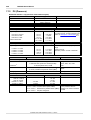
1.7 Software
...................................................................................................................................
requirements
26
Startup
2.1 CD-Contents
................................................................................................................................... 27
2.1.1 Setup-Program
.........................................................................................................................................................
2.1.2 Driver-software
.........................................................................................................................................................
for the PC / CAN-Bus interface
27
27
2.2 Interface
...................................................................................................................................
cards
27
2.2.1 IXXAT
.........................................................................................................................................................
interface cards
2.2.2 dSPACE
.........................................................................................................................................................
interface cards
2.2.3 KVASER
.........................................................................................................................................................
interface cards
2.2.4 Vector
.........................................................................................................................................................
interface cards
28
28
28
28
2.3 imc interface
...................................................................................................................................
adapter
29
2.3.1 Installation
.........................................................................................................................................................
of the imc-CAN/USB Adapter
2.3.2 Firmware
.........................................................................................................................................................
of the imc-CAN/USB Adapter
29
30
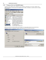
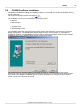
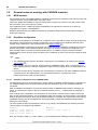
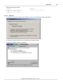
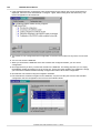
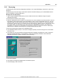
2.4 CANSAS
...................................................................................................................................
software installation
31
© 2011 imc Meßsysteme GmbH
3
2.5 Connections
................................................................................................................................... 33
2.5.1 CAN.........................................................................................................................................................
connection for the PC
2.5.2 CAN.........................................................................................................................................................
connection to CANSAS
2.5.3 CANSAS
.........................................................................................................................................................
analog connections
2.5.4 Checking
.........................................................................................................................................................
connections
33
34
34
34
2.6 Integrating
...................................................................................................................................
the CANSAS software with imcDevices
35
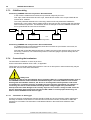
2.7 CAN-Bus
...................................................................................................................................
description
35
2.7.1 References
.........................................................................................................................................................
to standards and literature
2.7.2 Bus-activation
.........................................................................................................................................................
2.7.3 CAN-Bus-wiring
.........................................................................................................................................................
2.7.4 Connecting
.........................................................................................................................................................
the terminators
2.7.4.1 Termination
..................................................................................................................................................
in data logger
2.7.4.2 Termination
..................................................................................................................................................
with µ-CANSAS
2.7.5 Reset-plug
.........................................................................................................................................................
2.7.6 CAN.........................................................................................................................................................
data transfer rate
2.7.7 Number
.........................................................................................................................................................
of CAN-nodes
2.7.8 Duplicate
.........................................................................................................................................................
samples in during data capture
2.7.9 CANopen
.........................................................................................................................................................
2.7.9.1 Limitations
..................................................................................................................................................
2.7.10 Troubleshooting
.........................................................................................................................................................
tips for disturbances of the CAN-Bus
2.7.11 Cabling
.........................................................................................................................................................
of µ-CANSAS
2.7.11.1 Power
..................................................................................................................................................
from external power supply unit
2.7.11.2 Power
..................................................................................................................................................
supply from busDAQ unit
35
35
36
36
36
37
38
38
39
39
40
40
41
44
44
46
Operation
3.1 Calling
...................................................................................................................................
the program
47
3.1.1 Language
.........................................................................................................................................................
setting - imcLanguageSelector
47
3.2 The user
...................................................................................................................................
interface
48
3.2.1 Introduction
.........................................................................................................................................................
3.2.1.1 "File"..................................................................................................................................................
menu
3.2.1.2 "Edit"..................................................................................................................................................
menu
3.2.1.3 "View"..................................................................................................................................................
menu
3.2.1.4 "Module"..................................................................................................................................................
menu
3.2.1.5 "Extra"..................................................................................................................................................
menu
3.2.1.6 "?"..................................................................................................................................................
menu (Help)
3.2.1.7 Control
..................................................................................................................................................
Menu
3.2.2 Toolbar
.........................................................................................................................................................
3.2.3 The .........................................................................................................................................................
Module Tree
3.2.4 Properties
.........................................................................................................................................................
Display
3.2.4.1 Module
..................................................................................................................................................
database
3.2.4.2 CANSAS
..................................................................................................................................................
Module
3.2.4.2.1 General
...........................................................................................................................................
3.2.4.2.2 Version
...........................................................................................................................................
3.2.4.2.3 SlotInfo
...........................................................................................................................................
3.2.4.2.4 Sensors
...........................................................................................................................................
3.2.4.3 CAN-Bus
..................................................................................................................................................
Interface
3.2.4.4 CAN-Bus
..................................................................................................................................................
message
3.2.4.5 Input/Output
..................................................................................................................................................
stage
3.2.4.6 Input
..................................................................................................................................................
channel
3.2.4.6.1 Third
...........................................................................................................................................
output module dialog
3.2.4.7 Virtual
..................................................................................................................................................
channels
3.2.4.8 Virtual
..................................................................................................................................................
channel
© 2011 imc Meßsysteme GmbH
48
49
49
50
50
50
51
51
52
53
54
54
56
56
57
58
58
59
61
62
63
66
67
67
4
CANSAS Users Manual
3.2.4.9 Special
..................................................................................................................................................
functions
3.2.5 Status
.........................................................................................................................................................
bar
69
69
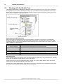
3.3 Working
...................................................................................................................................
with the Module Tree
70
3.4 Menu...................................................................................................................................
functions
73
3.4.1 Files.........................................................................................................................................................
3.4.1.1 File
..................................................................................................................................................
- New
3.4.1.2 File
..................................................................................................................................................
- Open...
3.4.1.3 File
..................................................................................................................................................
- Save
3.4.1.4 File
..................................................................................................................................................
- Save as...
3.4.1.5 File
..................................................................................................................................................
- Import
3.4.1.6 File
..................................................................................................................................................
- Export...
3.4.1.7 File
..................................................................................................................................................
- Print
3.4.1.8 File
..................................................................................................................................................
- Page Preview
3.4.1.8.1 The
...........................................................................................................................................
'Print' dialog
3.4.1.8.2 The
...........................................................................................................................................
'Export' dialog
3.4.1.9 File
..................................................................................................................................................
- Print Setup...
3.4.1.9.1 The
...........................................................................................................................................
'Print Setup' dialog
3.4.1.10 File
..................................................................................................................................................
- Close
3.4.2 Edit .........................................................................................................................................................
3.4.2.1 Edit
..................................................................................................................................................
- Undo
3.4.2.2 Edit
..................................................................................................................................................
- Cut
3.4.2.3 Edit
..................................................................................................................................................
- copy
3.4.2.4 Edit
..................................................................................................................................................
- Paste
3.4.2.5 Edit
..................................................................................................................................................
- New
3.4.2.6 Edit
..................................................................................................................................................
- Rename
3.4.2.7 Edit
..................................................................................................................................................
- Delete
3.4.3 View.........................................................................................................................................................
3.4.3.1 View
..................................................................................................................................................
- Toolbar
3.4.3.2 View
..................................................................................................................................................
- Status bar
3.4.3.3 View
..................................................................................................................................................
- Split
3.4.3.4 View
..................................................................................................................................................
- Adjust
3.4.3.5 View
..................................................................................................................................................
- Group by
3.4.3.6 View
..................................................................................................................................................
- Expand all branches/Collapse all branches
3.4.4 Module
.........................................................................................................................................................
3.4.4.1 Module
..................................................................................................................................................
- Integrating Assistant
3.4.4.2 Module
..................................................................................................................................................
- Find selections...
3.4.4.3 Module
..................................................................................................................................................
- Check configuration
3.4.4.4 Module
..................................................................................................................................................
- Configure...
3.4.4.5 Module
..................................................................................................................................................
- Measure...
3.4.4.6 Module
..................................................................................................................................................
- Two-point-Scaling
3.4.4.7 Module
..................................................................................................................................................
- Sensors
3.4.4.8 Module
..................................................................................................................................................
- Calculate Bus load
3.4.5 Extra
.........................................................................................................................................................
3.4.5.1 Extras
..................................................................................................................................................
- Interface
3.4.5.2 Extras
..................................................................................................................................................
- Options
3.4.5.2.1 Module
...........................................................................................................................................
3.4.5.2.2 Sensor
...........................................................................................................................................
3.4.5.2.3 Export
...........................................................................................................................................
3.4.5.2.4 Display
...........................................................................................................................................
3.4.5.2.5 General
...........................................................................................................................................
3.4.6 Help.........................................................................................................................................................
- Info about CANSAS...
73
73
73
73
73
74
74
74
75
75
76
77
77
77
77
77
77
78
78
78
79
79
79
79
79
79
80
80
80
81
81
85
86
87
88
89
91
91
92
92
94
94
95
96
96
97
97
3.5 General
...................................................................................................................................
notes on working with CANSAS modules
98
3.5.1 MDB.........................................................................................................................................................
database
98
© 2011 imc Meßsysteme GmbH
5
3.5.2 Readable
.........................................................................................................................................................
configuration
3.5.2.1 Readable
..................................................................................................................................................
configuration for µ-CANSAS-HUB4
3.5.2.2 Operation
..................................................................................................................................................
3.5.3 Reset-plug
.........................................................................................................................................................
3.5.4 Bus-off
.........................................................................................................................................................
error - Change baudrate
3.5.5 Racks
.........................................................................................................................................................
3.5.5.1 Racks,
..................................................................................................................................................
slot identification
3.5.5.2 Using
..................................................................................................................................................
CANSAS in a rack
3.5.5.3 Rack
..................................................................................................................................................
maintenance
3.5.5.4 Operating
..................................................................................................................................................
software, modification of the Baud rate
3.5.6 Connecting
.........................................................................................................................................................
to "imc-Sensors"
3.5.7 Sensor
.........................................................................................................................................................
recognition
3.5.8 Guarding
.........................................................................................................................................................
3.5.9 Heartbeats
.........................................................................................................................................................
3.5.10 Synchronization
.........................................................................................................................................................
98
98
99
101
103
104
104
104
105
105
107
108
110
111
112
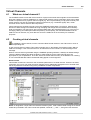
Virtual Channels
4.1 What...................................................................................................................................
are virtual channels?
115
4.2 Creating
...................................................................................................................................
virtual channels
115
4.3 Data...................................................................................................................................
formats
117
4.4 Integer-arithmetic
................................................................................................................................... 117
4.5 Constraints
................................................................................................................................... 118
4.6 LEDs
................................................................................................................................... 118
4.7 Special
...................................................................................................................................
module-specific characteristics
119
4.7.1 Acquisition
.........................................................................................................................................................
modules
4.7.1.1 ISO8,
..................................................................................................................................................
C8, INC4 and C12
4.7.1.2 BRIDGE2
..................................................................................................................................................
4.7.1.3 P8
..................................................................................................................................................
4.7.1.4 UNI8
..................................................................................................................................................
4.7.1.5 DI16
..................................................................................................................................................
4.7.2 Output
.........................................................................................................................................................
modules
4.7.2.1 DAC8
..................................................................................................................................................
4.7.2.2 PWM8
..................................................................................................................................................
4.7.2.3 DO8R,
..................................................................................................................................................
DO16R
119
120
120
121
121
121
121
122
122
122
4.8 Sampling
...................................................................................................................................
Rates
123
4.9 Processing
...................................................................................................................................
functions sorted by group
124
4.10 Function
...................................................................................................................................
Reference
125
4.10.1 + (Addition)
.........................................................................................................................................................
4.10.2 - (Subtraction)
.........................................................................................................................................................
4.10.3 - (Negative
.........................................................................................................................................................
sign)
4.10.4 * (Multiplication)
.........................................................................................................................................................
4.10.5 / (Division)
.........................................................................................................................................................
4.10.6 1/x
.........................................................................................................................................................
(Inverse)
4.10.7 Absolute
.........................................................................................................................................................
value
4.10.8 Assignment
.........................................................................................................................................................
4.10.9 Band-pass
.........................................................................................................................................................
filter
4.10.10 Barometer
.........................................................................................................................................................
(only for P8 modules)
4.10.11 Bitwise
.........................................................................................................................................................
AND
4.10.12 Bitwise
.........................................................................................................................................................
NOT
4.10.13 Bitwise
.........................................................................................................................................................
OR
© 2011 imc Meßsysteme GmbH
125
125
126
126
126
127
127
127
128
128
129
129
130
6
CANSAS Users Manual
4.10.14 Bitwise
.........................................................................................................................................................
exclusive OR
4.10.15 Button
.........................................................................................................................................................
status (only for BRIGDE2 and UNI8 modules)
4.10.16 Channel-status
.........................................................................................................................................................
word (only for UNI8 and CI8 modules)
4.10.17 Characteristic
.........................................................................................................................................................
curve
4.10.18 Comparison
.........................................................................................................................................................
function
4.10.19 Constant
.........................................................................................................................................................
channel (only for acquisition modules)
4.10.20 Constant
.........................................................................................................................................................
digital channel
4.10.21 Conversion
.........................................................................................................................................................
to Float numerical format (only for acquisition modules)
4.10.22 Event
.........................................................................................................................................................
counting (only for DI16 modules)
4.10.23 Exp.
.........................................................................................................................................................
root mean square (RMS)
4.10.24 Extract
.........................................................................................................................................................
bit from word
4.10.25 Fixed
.........................................................................................................................................................
analog value (only for DAC8 and PWM8 modules)
4.10.26 Fixed
.........................................................................................................................................................
digital value (only for digital output modules)
4.10.27 Fixed
.........................................................................................................................................................
input range
4.10.28 Fixed
.........................................................................................................................................................
scaling
4.10.29 Frequency
.........................................................................................................................................................
determination (only for DI16 modules)
4.10.30 Greater
.........................................................................................................................................................
4.10.31 Greater
.........................................................................................................................................................
value
4.10.32 High-pass
.........................................................................................................................................................
filter
4.10.33 Hysteresis
.........................................................................................................................................................
filter
4.10.34 LED-flash
.........................................................................................................................................................
4.10.35 Less
.........................................................................................................................................................
4.10.36 Less
.........................................................................................................................................................
value
4.10.37 Logical
.........................................................................................................................................................
AND
4.10.38 Logical
.........................................................................................................................................................
NOT
4.10.39 Logical
.........................................................................................................................................................
OR
4.10.40 Logical
.........................................................................................................................................................
exclusive OR
4.10.41 Low-pass
.........................................................................................................................................................
filter
4.10.42 Maximum
.........................................................................................................................................................
4.10.43 Mean
.........................................................................................................................................................
value
4.10.44 Median
.........................................................................................................................................................
filter
4.10.45 Minimum
.........................................................................................................................................................
4.10.46 Module-status
.........................................................................................................................................................
word (only for UNI8 and CI8 modules)
4.10.47 Monoflop
.........................................................................................................................................................
4.10.48 Output
.........................................................................................................................................................
status on LED (only for BRIDGE2, UNI8 and CI8 modules)
4.10.49 Output
.........................................................................................................................................................
status word (only for BRIDGE2, C8, P8, INC4 and SC modules)
4.10.50 PulseSequenceEncoder
.........................................................................................................................................................
(only for output modules)
4.10.51 Rectangle
.........................................................................................................................................................
(only for DAC8 modules)
4.10.52 Resampling
.........................................................................................................................................................
4.10.53 Root-mean-square
.........................................................................................................................................................
4.10.54 SawTooth
.........................................................................................................................................................
4.10.55 Schmitt-Trigger
.........................................................................................................................................................
4.10.56 Short
.........................................................................................................................................................
circuit status (only for BRIDGE2 and UNI8 modules)
4.10.57 Sine
.........................................................................................................................................................
(only for DAC8 modules)
4.10.58 Slope
.........................................................................................................................................................
limiting
4.10.59 Smoothing
.........................................................................................................................................................
based on 2 values
4.10.60 Smoothing
.........................................................................................................................................................
based on 3 values
4.10.61 Square
.........................................................................................................................................................
root
4.10.62 Standard
.........................................................................................................................................................
deviation
4.10.63 Time
.........................................................................................................................................................
determination (only for DI16 modules)
4.10.64 Triangle
.........................................................................................................................................................
(only for DAC8 modules)
130
131
131
132
133
133
133
134
134
134
135
135
136
136
136
137
138
138
139
139
140
141
141
142
142
143
143
144
144
145
145
145
146
146
147
148
149
149
150
150
150
151
151
152
152
152
153
153
153
154
155
Measurement Technique
5.1 Measurement
...................................................................................................................................
modes
156
© 2011 imc Meßsysteme GmbH
7
5.1.1 Bridge
.........................................................................................................................................................
modules
5.1.1.1 General
..................................................................................................................................................
remarks
5.1.2 Bridge
.........................................................................................................................................................
measurements with wire strain gauges (WSGs)
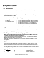
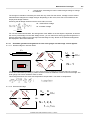
5.1.2.1 Selectable geometric arrangements for wire strain gauges and the
bridge circuits
..................................................................................................................................................
applied:
5.1.2.1.1...........................................................................................................................................
Quarter bridge for 120 Ohm WSG
5.1.2.1.2...........................................................................................................................................
General half bridge
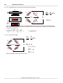
5.1.2.1.3...........................................................................................................................................
Poisson half bridge
5.1.2.1.4...........................................................................................................................................
Half bridge with two active strain gauges in uniaxial direction
5.1.2.1.5...........................................................................................................................................
Half bridges with one active and one passive strain gauge
5.1.2.1.6...........................................................................................................................................
General Full bridge
5.1.2.1.7...........................................................................................................................................
Full bridge with Poisson strain gauges in opposed branches
5.1.2.1.8...........................................................................................................................................
Full bridge with Poisson strain gauges in adjacent branches
5.1.2.1.9...........................................................................................................................................
Full bridge with 4 active strain gauges in uniaxial direction
5.1.2.1.10 Full bridge (Half bridge-shear strain) opposite arms two
active strain
...........................................................................................................................................
gauges
5.1.2.1.11
...........................................................................................................................................
Scaling for the strain analysis
5.1.2.2 Bridge
..................................................................................................................................................
balancing
5.1.3 Incremental
.........................................................................................................................................................
encoders
5.1.3.1 Connections
..................................................................................................................................................
5.1.3.2 Comparator
..................................................................................................................................................
conditioning
5.1.3.3 Block
..................................................................................................................................................
diagram
5.1.3.4 Single-signal/
..................................................................................................................................................
Two-signal
5.1.3.5 Zero
..................................................................................................................................................
pulse (index)
5.1.3.6 Missing
..................................................................................................................................................
tooth
5.1.3.7 Event
..................................................................................................................................................
counting, angle and displacement measurement
5.1.3.7.1...........................................................................................................................................
Resetting of summation
5.1.3.8 Time
..................................................................................................................................................
measurement
5.1.3.9 PWM
..................................................................................................................................................
5.1.3.10..................................................................................................................................................
Measurements of frequency, RPMs and velocity
5.1.3.11..................................................................................................................................................
Data types
5.1.4 Digital
.........................................................................................................................................................
Inputs
5.1.5 Digital
.........................................................................................................................................................
Outputs (CANSAS-DO8R, -DO16, -DO16R)
5.1.5.1 Outputs
..................................................................................................................................................
5.1.5.2 Connecting
..................................................................................................................................................
an output signal with a CAN-message
5.1.5.3 Calculated
..................................................................................................................................................
output signals
5.1.5.4 Notes
..................................................................................................................................................
on DO8R and DO16R
5.1.5.5 Taking
..................................................................................................................................................
measurements with the digital output modules
5.1.6 Temperature
.........................................................................................................................................................
measurement
5.1.6.1 Thermocouples
..................................................................................................................................................
as per DIN and IEC
5.1.6.2 Pt100
..................................................................................................................................................
(RTD) - measurement
5.1.6.3 imc
..................................................................................................................................................
thermo plug
5.1.6.3.1 Schematic: imc-Thermoplug (ACC/DSUB-T4) with isolated
voltage channels
...........................................................................................................................................
156
156
156
157
157
157
159
159
160
160
161
161
162
162
163
164
164
164
165
166
166
166
167
167
168
170
171
173
174
175
175
175
175
176
178
178
179
179
180
180
181
5.2 Sampling
...................................................................................................................................
rates: Scanner concept
182
5.3 CAN-Bus:
...................................................................................................................................
Delay times
184
5.4 Isolation,
...................................................................................................................................
Grounding and Shielding
185
5.4.1 Isolation
.........................................................................................................................................................
5.4.2 Grounding
.........................................................................................................................................................
5.4.3 Isolation
.........................................................................................................................................................
voltage
5.4.4 Shielding
.........................................................................................................................................................
185
185
186
187
5.5 CANSAS
...................................................................................................................................
blinking codes
188
5.5.1 Normal
.........................................................................................................................................................
operation
5.5.1.1 Successful
..................................................................................................................................................
configuration
© 2011 imc Meßsysteme GmbH
188
188
8
CANSAS Users Manual
5.5.1.2 With
..................................................................................................................................................
device's Reset-plug
5.5.1.3 Synchronization
..................................................................................................................................................
5.5.1.4 Fault
..................................................................................................................................................
condition in device
5.5.1.5 UNI8
..................................................................................................................................................
- TEDS
5.5.1.6 Canser
..................................................................................................................................................
GPS
5.5.1.7 µ-CANSAS
..................................................................................................................................................
and µ-CANSAS-HUB4
188
188
189
190
190
190
5.6 Features
...................................................................................................................................
and modules
192
5.7 Calibrating
...................................................................................................................................
the modules
194
5.7.1 Prompt
.........................................................................................................................................................
for next calibration
5.7.2 Recalibration
.........................................................................................................................................................
overdue
194
196
5.8 TEDS
................................................................................................................................... 199
5.8.1 TEDS:
.........................................................................................................................................................
Plug & Measure functionality for sensors
5.8.1.1 How
..................................................................................................................................................
can measurement be simplified for the user?
5.8.1.2 Steps
..................................................................................................................................................
Towards Achieving "Plug & Measure" Functionality
5.8.1.3 Sensor
..................................................................................................................................................
database
5.8.2 Operation
.........................................................................................................................................................
in CANSAS Software
5.8.2.1 Importing
..................................................................................................................................................
sensor data
5.8.2.2 Sensor
..................................................................................................................................................
information
5.8.2.3 Saving
..................................................................................................................................................
imported sensor information in CANSAS
5.8.2.4 Sensor-Database
..................................................................................................................................................
5.8.2.4.1...........................................................................................................................................
Importing sensor information from the sensor database
5.8.2.4.2 Exchanging sensor information between the sensor-Eprom
and sensor
...........................................................................................................................................
database
5.8.2.4.3...........................................................................................................................................
Read Sensor-Eprom
5.8.2.4.4...........................................................................................................................................
Write Sensor-Eprom
5.8.3 Plug
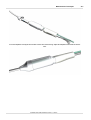
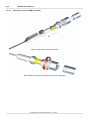
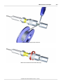
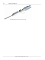
.........................................................................................................................................................
& Measure - Assembly of the sensor clip
5.8.3.1 Assembly
..................................................................................................................................................
of the ITT-VEAM plug (UNI8)
199
199
199
201
203
204
204
205
205
205
207
208
208
209
212
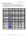
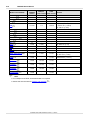
Properties of the Modules
6.1 BRIDGE2
................................................................................................................................... 217
6.1.1 DC-.........................................................................................................................................................
bridge readings (measurement target: Sensor)
6.1.2 Full.........................................................................................................................................................
bridge
6.1.3 Half.........................................................................................................................................................
bridge
6.1.4 Quarter
.........................................................................................................................................................
bridge
6.1.5 Balancing
.........................................................................................................................................................
and shunt calibration
6.1.5.1 Performing
..................................................................................................................................................
bridge balance by button
6.1.5.2 Bridge
..................................................................................................................................................
balance upon power-up of CANSAS-BRIDGE2
6.1.5.3 Activating
..................................................................................................................................................
bridge balance via Can-bus
6.1.5.4 Bridge
..................................................................................................................................................
balance duration
6.1.5.5 Shunt
..................................................................................................................................................
calibration
6.1.6 Connector
.........................................................................................................................................................
plugs BRIDGE2
6.1.7 Sampling
.........................................................................................................................................................
interval
219
220
221
222
223
224
224
224
224
225
226
226
6.2 CANSER-GPS
................................................................................................................................... 227
6.2.1 Use.........................................................................................................................................................
of CANSER-GPS
6.2.2 LED
.........................................................................................................................................................
signals of CANSER-module status:
227
227
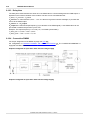
6.3 C12 ...................................................................................................................................
voltage, temperature, current
228
6.3.1 Connector
.........................................................................................................................................................
plugs C12
230
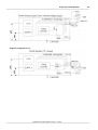
6.4 C8 voltage,
...................................................................................................................................
temperature, current
231
6.4.1 Voltage
.........................................................................................................................................................
measurement
6.4.2 Current
.........................................................................................................................................................
measurement
6.4.3 Temperature
.........................................................................................................................................................
measurement
6.4.3.1 imc
..................................................................................................................................................
thermoplug (type: Standard DSUB)
231
232
233
233
© 2011 imc Meßsysteme GmbH
9
6.4.3.2 Measurement
..................................................................................................................................................
with PT100 (RTD) (Type: Standard DSUB)
6.4.3.3 Measurement
..................................................................................................................................................
with PT100 (RTD) (Type: LEMO)
6.4.3.4 Thermocouple
..................................................................................................................................................
measurement (Type II: round plugs)
6.4.4 Module
.........................................................................................................................................................
Sensor SUPPLY
6.4.5 Sampling
.........................................................................................................................................................
intervals, filters and anti-aliasing
6.4.6 Connector
.........................................................................................................................................................
plugs C8
6.4.6.1 Standard
..................................................................................................................................................
variety (DSUB-15)
6.4.6.2 Variety
..................................................................................................................................................
I (5-pin Fischer round plugs)
6.4.6.3 SL
..................................................................................................................................................
Variety LEMO
233
234
234
234
235
237
237
237
237
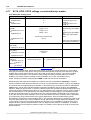
6.5 CI8 isolated
...................................................................................................................................
voltage channels with current and temperature mode
238
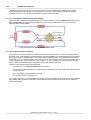
6.5.1 Voltage
.........................................................................................................................................................
measurement
6.5.1.1 Voltage
..................................................................................................................................................
measurement with zero balancing
6.5.2 Current
.........................................................................................................................................................
measurement
6.5.3 Temperature
.........................................................................................................................................................
measurement
6.5.3.1 Measurement
..................................................................................................................................................
with PT100 (RTD) (Type LEMO)
6.5.4 Resistance
.........................................................................................................................................................
measurement
6.5.5 Optional
.........................................................................................................................................................
sensor supply module
6.5.6 Allow
.........................................................................................................................................................
overmodulation beyond input range
6.5.7 Filter
.........................................................................................................................................................
6.5.8 Connector
.........................................................................................................................................................
plugs CI8
6.5.8.1 SL
..................................................................................................................................................
Variety LEMO
239
239
242
243
243
244
244
245
246
247
247
6.6 DAC8
...................................................................................................................................
analog outputs
247
6.6.1 General
.........................................................................................................................................................
notes DAC8
6.6.2 Analog
.........................................................................................................................................................
portion
6.6.3 Linking
.........................................................................................................................................................
the output signal to a CAN-message
6.6.4 Message
.........................................................................................................................................................
Mapping
6.6.5 Calculating
.........................................................................................................................................................
the output signal
6.6.6 Configuring
.........................................................................................................................................................
the outputs
6.6.7 CANSAS-DAC8
.........................................................................................................................................................
block diagram
6.6.8 Taking
.........................................................................................................................................................
measurements with the analog output modules
6.6.9 Connector
.........................................................................................................................................................
plugs DAC8
6.6.9.1 Pin
..................................................................................................................................................
configuration ITT VEAM (CANSAS-L-DAC8-V)
247
247
248
249
249
251
251
252
252
252
6.7 DCB8
................................................................................................................................... 253
6.7.1 Bridge
.........................................................................................................................................................
measurement
6.7.1.1 Full
..................................................................................................................................................
bridge
6.7.1.2 Half
..................................................................................................................................................
bridge
6.7.1.3 Quarter
..................................................................................................................................................
bridge
6.7.1.4 Sense
..................................................................................................................................................
and initial unbalance
6.7.1.5 Balancing
..................................................................................................................................................
and shunt calibration
6.7.2 Voltage
.........................................................................................................................................................
measurement
6.7.2.1 Voltage
..................................................................................................................................................
source with ground reference
6.7.2.2 Voltage
..................................................................................................................................................
source without ground reference
6.7.2.3 Voltage
..................................................................................................................................................
source at a different fixed potential
6.7.2.4 Voltage
..................................................................................................................................................
measurement: With zero-adjusting (tare)
6.7.3 Sensor
.........................................................................................................................................................
supply
6.7.4 Bandwidth
.........................................................................................................................................................
253
254
254
255
256
256
257
257
258
258
258
259
259
6.8 DI16...................................................................................................................................
digital inputs
259
6.8.1 Overview
.........................................................................................................................................................
6.8.2 Settings
.........................................................................................................................................................
6.8.3 Block
.........................................................................................................................................................
diagram
6.8.4 Sampling
.........................................................................................................................................................
Interval
6.8.5 CAN-bus
.........................................................................................................................................................
message dialog
6.8.6 Connector
.........................................................................................................................................................
plugs DI16
© 2011 imc Meßsysteme GmbH
259
260
260
261
261
262
10
CANSAS Users Manual
6.9 DO16
...................................................................................................................................
digital outputs
263
6.9.1 Configuring
.........................................................................................................................................................
the outputs
6.9.2 Starting
.........................................................................................................................................................
up the DO16 module
6.9.3 CANSAS-DO16
.........................................................................................................................................................
block diagram
6.9.3.1 Open
..................................................................................................................................................
Drain Mode
6.9.3.2 Totem-Pole
..................................................................................................................................................
Mode
6.9.4 Invert
.........................................................................................................................................................
Output
6.9.5 Connector
.........................................................................................................................................................
plugs DO16
263
263
263
263
264
264
265
6.10 DO8R,
...................................................................................................................................
-DO16R relay outputs
266
6.10.1 block
.........................................................................................................................................................
diagram DO8R, DO16R
6.10.2 Starting
.........................................................................................................................................................
the DO8R, DO16R module
6.10.3 Connector
.........................................................................................................................................................
plugs DO8R, DO16R
266
266
266
6.11 IGN...................................................................................................................................
ignition angle measurement module
267
6.11.1 Interference
.........................................................................................................................................................
suppression
6.11.2 Housing
.........................................................................................................................................................
6.11.2.1..................................................................................................................................................
Grounding bolt
6.11.2.2..................................................................................................................................................
LEDs
6.11.2.3..................................................................................................................................................
Display
6.11.3 Operation
.........................................................................................................................................................
modes
6.11.3.1..................................................................................................................................................
Default operation type
6.11.3.1.1
...........................................................................................................................................
Message
6.11.3.2..................................................................................................................................................
Snapshot operation mode
6.11.3.2.1
...........................................................................................................................................
Message
6.11.4 Parameterization
.........................................................................................................................................................
6.11.4.1..................................................................................................................................................
The channel's parameters
6.11.4.2..................................................................................................................................................
Offset adjustment
6.11.5 Tips
.........................................................................................................................................................
6.11.6 IGN
.........................................................................................................................................................
terminal
6.11.6.1..................................................................................................................................................
Inputs (BNC)
6.11.6.2..................................................................................................................................................
Outputs (DSUB9)
271
271
271
271
271
272
272
272
272
274
275
279
281
282
284
284
284
6.12 INC4
...................................................................................................................................
incremental encoder channels
286
6.12.1 Measurement
.........................................................................................................................................................
quantities
6.12.2 Comparator
.........................................................................................................................................................
configuration
6.12.3 Sensor
.........................................................................................................................................................
types, synchronization
6.12.4 Sensors
.........................................................................................................................................................
with current signals
6.12.5 Sensor
.........................................................................................................................................................
supply at L-INC4-V-SUPPLY
6.12.6 Connector
.........................................................................................................................................................
plugs
286
287
289
289
290
290
6.13 ISO8
...................................................................................................................................
isolated voltage channels with current and temp. modes
291
6.13.1 Connector
.........................................................................................................................................................
plugs ISO8
291
6.14 HCI8
...................................................................................................................................
isolated voltage, current, resistor, temperature
292
6.14.1 Voltage
.........................................................................................................................................................
measurement
6.14.2 Current
.........................................................................................................................................................
measurement
6.14.3 Temperature
.........................................................................................................................................................
measurement
6.14.3.1..................................................................................................................................................
Thermocouple measurement
6.14.3.2..................................................................................................................................................
Pt100 (RTD) - Measurement
6.14.4 Resistance
.........................................................................................................................................................
measurement
6.14.5 Bandwidth
.........................................................................................................................................................
6.14.6 Connection
.........................................................................................................................................................
293
294
295
295
296
296
297
297
6.15 P8 ...................................................................................................................................
pressure
298
6.15.1 General
.........................................................................................................................................................
remarks
6.15.2 Absolute
.........................................................................................................................................................
and relative pressure
6.15.3 Barometer
.........................................................................................................................................................
299
299
299
© 2011 imc Meßsysteme GmbH
11
6.15.4 Sensors
.........................................................................................................................................................
6.15.5 Factors
.........................................................................................................................................................
affecting pressure measurement
6.15.6 Sampling
.........................................................................................................................................................
intervals, filters and anti-aliasing
6.15.7 Operating
.........................................................................................................................................................
software
6.15.7.1..................................................................................................................................................
Module integration
6.15.7.2..................................................................................................................................................
Read-in of sensor data
6.15.7.3..................................................................................................................................................
Measurement mode
6.15.7.4..................................................................................................................................................
Balancing
6.15.7.5..................................................................................................................................................
Barometer
6.15.7.5.1
...........................................................................................................................................
Barometer readings
6.15.7.5.2
...........................................................................................................................................
Built-in error recognition ("Min/Max values"):
6.15.8 Maintenance
.........................................................................................................................................................
6.15.9 Pressure
.........................................................................................................................................................
terminals, aggressive media
6.15.10 Table
.........................................................................................................................................................
of Chemical Resistance
6.15.11 Pin
.........................................................................................................................................................
configuration of CANSAS-P8-IP65
6.15.12 CANSAS-IP65-P8-E
.........................................................................................................................................................
6.15.13 Grounding
.........................................................................................................................................................
299
300
301
302
302
302
303
304
305
306
306
307
308
308
312
312
313
6.16 PWM8
...................................................................................................................................
pulse width modulation outputs
313
6.16.1 8 PWM
.........................................................................................................................................................
outputs
6.16.2 Scaling
.........................................................................................................................................................
6.16.3 Delay
.........................................................................................................................................................
time
6.16.4 Connection
.........................................................................................................................................................
PWM8
313
315
316
316
6.17 SC16,
...................................................................................................................................
SCI8, SCI16 voltage, current and temp. modes
318
6.17.1 Voltage
.........................................................................................................................................................
measurement
6.17.2 Current
.........................................................................................................................................................
measurement
6.17.3 Temperature
.........................................................................................................................................................
measurement
6.17.3.1..................................................................................................................................................
Thermocouple measurement
6.17.3.2..................................................................................................................................................
PT100 (RTD) - Measurement
6.17.3.3..................................................................................................................................................
PT100 (RTD) - Measurement (Type: LEMO)
6.17.3.4..................................................................................................................................................
Probe-breakage recognition
6.17.3.5..................................................................................................................................................
Deactivate probe-breakage recognition
6.17.4 External
.........................................................................................................................................................
sensor supply (optional)
6.17.5 Connector
.........................................................................................................................................................
plugs SC16, SCI8, SCI16
6.17.5.1..................................................................................................................................................
SL Variety LEMO
6.17.6 Sampling
.........................................................................................................................................................
rates
6.17.7 Isolation
.........................................................................................................................................................
- Concept
6.17.8 Isolation
.........................................................................................................................................................
of the voltage supply module
6.17.9 Filter
.........................................................................................................................................................
6.17.9.1..................................................................................................................................................
SC16 Filter
6.17.9.2..................................................................................................................................................
SCI16 Filter
6.17.9.3..................................................................................................................................................
SCI8 Filter
6.17.10 Delay
.........................................................................................................................................................
319
320
321
321
321
322
322
323
324
324
325
325
325
326
327
329
330
331
332
6.18 UNI8
................................................................................................................................... 333
6.18.1 Voltage
.........................................................................................................................................................
measurement
6.18.1.1..................................................................................................................................................
Voltage source with ground reference
6.18.1.2..................................................................................................................................................
Voltage source without ground reference
6.18.1.3..................................................................................................................................................
Voltage source at a different fixed potential
6.18.1.4..................................................................................................................................................
Voltage measurement: with zero-adjusting (tare)
6.18.2 Bridge
.........................................................................................................................................................
measurement
6.18.2.1..................................................................................................................................................
Full bridge
6.18.2.2..................................................................................................................................................
Half bridge
6.18.2.3..................................................................................................................................................
Quarter bridge
6.18.2.4..................................................................................................................................................
Sense and initial unbalance
© 2011 imc Meßsysteme GmbH
334
335
335
336
336
337
337
338
338
339
12
CANSAS Users Manual
6.18.2.5..................................................................................................................................................
Balancing and shunt calibration
6.18.3 Current
.........................................................................................................................................................
measurement
6.18.3.1..................................................................................................................................................
Differential current measurement
6.18.3.2..................................................................................................................................................
Ground-referenced current measurement
6.18.3.3..................................................................................................................................................
2-wire for sensors with a current signal and variable supply
6.18.4 Temperature
.........................................................................................................................................................
measurement
6.18.4.1..................................................................................................................................................
Thermocouple measurement
6.18.4.1.1
...........................................................................................................................................
Thermocouple mounted with ground reference
6.18.4.1.2
...........................................................................................................................................
Thermocouple mounted without ground reference
6.18.4.2..................................................................................................................................................
Pt100/ RTD measurement
6.18.4.2.1
...........................................................................................................................................
Pt100 in 4-wire configuration
6.18.4.2.2
...........................................................................................................................................
Pt100 in 2-wire configuration
6.18.4.2.3
...........................................................................................................................................
Pt100 in 3-wire configuration
6.18.4.3..................................................................................................................................................
Probe-breakage recognition
6.18.5 Resistance
.........................................................................................................................................................
measurement
6.18.6 Sensors
.........................................................................................................................................................
requiring adjustment of their supply
6.18.7 Sensor
.........................................................................................................................................................
supply module
6.18.8 Bandwidth
.........................................................................................................................................................
6.18.9 Sampling
.........................................................................................................................................................
intervals, filters and anti-aliasing
6.18.10 Recognition
.........................................................................................................................................................
of sensor by means of wire jumpers
6.18.11 Connector
.........................................................................................................................................................
plugs
6.18.11.1
..................................................................................................................................................
Pin configuration of round plugs ITT-VEAM (MIL-C-26482)
6.18.11.2
..................................................................................................................................................
Pin configuration of round plugs LEMOSA
6.18.11.3
..................................................................................................................................................
Pin configuration of round plugs ZF LEMO
6.18.12 Assembly
.........................................................................................................................................................
instructions for ITT VEAM with Pt100 inside of connector
6.18.12.1
..................................................................................................................................................
Connection using crimps
6.18.12.2
..................................................................................................................................................
Connection by soldering
6.18.12.3
..................................................................................................................................................
Recommended tools
6.18.13 UNI8/DCB8-PROTECT
.........................................................................................................................................................
339
340
340
341
341
342
342
343
344
344
345
345
345
346
346
347
347
348
348
349
350
351
352
352
353
354
354
354
355
6.19 µ-CANSAS-V1
................................................................................................................................... 355
6.19.1 Voltage
.........................................................................................................................................................
measurement
6.19.2 Voltage
.........................................................................................................................................................
measurement: With zero-adjusting
6.19.2.1..................................................................................................................................................
Balance upon power-up
6.19.2.2..................................................................................................................................................
Activating balance via CAN-bus
6.19.2.3..................................................................................................................................................
Voltage balancing via measurement window
6.19.3 Message
.........................................................................................................................................................
Mapping
6.19.4 External
.........................................................................................................................................................
Supply voltage +5 V/+10 V (isolated)
6.19.5 Sampling
.........................................................................................................................................................
interval, filter
6.19.6 µ-CANSAS-V1
.........................................................................................................................................................
connector
356
357
358
358
359
360
360
361
362
6.20 µ-CANSAS-T1
................................................................................................................................... 363
6.20.1 Temperature
.........................................................................................................................................................
measurement
6.20.2 Message
.........................................................................................................................................................
Mapping
6.20.3 Sampling
.........................................................................................................................................................
interval, filter
6.20.4 µ-CANSAS-T1
.........................................................................................................................................................
connector
363
364
364
364
6.21 µ-CANSAS-B1
................................................................................................................................... 365
6.21.1 DC-bridge
.........................................................................................................................................................
measurement
6.21.2 Full
.........................................................................................................................................................
bridge
6.21.3 Half
.........................................................................................................................................................
bridge
6.21.4 Bridge
.........................................................................................................................................................
balancing
6.21.4.1..................................................................................................................................................
Bridge balancing upon power-up
6.21.4.2..................................................................................................................................................
Perform bridge balancing via the CAN-bus
6.21.4.3..................................................................................................................................................
Balancing in the measurement window
6.21.5 Message
.........................................................................................................................................................
Mapping
365
367
368
369
370
370
371
372
© 2011 imc Meßsysteme GmbH
13
6.21.6 Sampling
.........................................................................................................................................................
interval, filter
6.21.7 µ-CANSAS-B1
.........................................................................................................................................................
connector
373
374
6.22 µ-CANSAS-V4
................................................................................................................................... 375
6.23 µ-CANSAS-T4
................................................................................................................................... 376
6.24 µ-CANSAS-B4
................................................................................................................................... 377
6.25 µ-CANSAS-HUB4
................................................................................................................................... 378
6.25.1 Synchronization
.........................................................................................................................................................
379
General Technical Specs
7.1 BRIDGE2
................................................................................................................................... 383
7.2 CANSER-GPS
................................................................................................................................... 384
7.3 C12 ................................................................................................................................... 385
7.4 C8 ................................................................................................................................... 387
7.5 CI8 ................................................................................................................................... 389
7.6 DAC8
................................................................................................................................... 392
7.7 DCB8
................................................................................................................................... 393
7.8 DI16................................................................................................................................... 396
7.9 DO16
................................................................................................................................... 397
7.10 DO8R,
...................................................................................................................................
DO16R
398
7.11 IGN................................................................................................................................... 399
7.12 INC4
................................................................................................................................... 401
7.13 ISO8
................................................................................................................................... 403
7.14 HCI8
................................................................................................................................... 405
7.15 P8 ...................................................................................................................................
(Pressure)
408
7.16 PWM8
................................................................................................................................... 410
7.17 SC16
................................................................................................................................... 411
7.18 SCI8,
...................................................................................................................................
SCI16
414
7.19 UNI8
................................................................................................................................... 418
7.20 µ-CAN
...................................................................................................................................
- V1/V4
422
7.21 µ-CAN
...................................................................................................................................
- T1/T4
424
7.22 µ-CAN
...................................................................................................................................
- B1/B4
425
7.23 µ-CAN
...................................................................................................................................
- HUB4
426
7.24 Sensor
...................................................................................................................................
SUPPLY module
427
7.25 Synchronization
...................................................................................................................................
line
428
7.26 Tables
...................................................................................................................................
and diagrams
428
7.26.1 Cable
.........................................................................................................................................................
resistance as function of length and cross-section
428
7.27 Accessories
................................................................................................................................... 429
7.27.1 DSUB-screw
.........................................................................................................................................................
terminals for measurement inputs
7.27.2 CAN-bus
.........................................................................................................................................................
accessories
7.27.3 CANSAS
.........................................................................................................................................................
power supply accessories
7.27.4 DSUB
.........................................................................................................................................................
connector for incremental sensors with current signals
© 2011 imc Meßsysteme GmbH
429
430
430
431
14
CANSAS Users Manual
Pin configuration and power
supply
8.1 CAN-Bus
...................................................................................................................................
connectors
432
8.1.1 Standard
.........................................................................................................................................................
module with DSUB9 CAN Bus connector
8.1.1.1 CAN-Bus
..................................................................................................................................................
wiring
8.1.1.2 Notes
..................................................................................................................................................
for the use of CANcabs
8.1.1.3 Specification
..................................................................................................................................................
of components used
8.1.2 SL .........................................................................................................................................................
modules CAN-Bus connectors
8.1.2.1 CAN-Bus
..................................................................................................................................................
pin configuration and contact wiring
8.1.3 µ-CANSAS
.........................................................................................................................................................
CAN-Bus connections with
8.1.3.1 CAN-Bus
..................................................................................................................................................
pin configuration and contact wiring
8.1.3.2 Cables
..................................................................................................................................................
for µ-CANSAS
433
434
435
435
436
436
437
437
438
8.2 Power
...................................................................................................................................
Supply
441
8.2.1 Standard
.........................................................................................................................................................
modules power supply
8.2.2 CANSAS
.........................................................................................................................................................
SL power supply
8.2.3 µ-CANSAS
.........................................................................................................................................................
power supply
441
442
443
8.3 Pin configuration
...................................................................................................................................
of the connectors
443
8.3.1 Standard
.........................................................................................................................................................
modules with DSUB15
8.3.1.1 Modules
..................................................................................................................................................
with CAN-terminals
8.3.1.2 Modules
..................................................................................................................................................
with ACC-terminals
8.3.1.3 TEDS
..................................................................................................................................................
plugs (ACC/DSUB-TEDS) DSUB-15 sockets
8.3.1.4 Connector
..................................................................................................................................................
plugs Cross-Reference
8.3.1.5 imc
..................................................................................................................................................
plugs
8.3.1.5.1...........................................................................................................................................
imc voltage plug
8.3.1.5.2...........................................................................................................................................
imc Thermo-plug
8.3.2 Pin.........................................................................................................................................................
configuration DSUB-9 connectors
8.3.2.1 CANSAS-K-INC4
..................................................................................................................................................
8.3.3 Modules
.........................................................................................................................................................
with ITT VEAM terminals
8.3.4 CANSAS-SL
.........................................................................................................................................................
with LEMO terminals
8.3.4.1 DCB8,
..................................................................................................................................................
UNI8 LEMO
8.3.4.2 C8,
..................................................................................................................................................
CI8, SCI8, SCI16, SC16 LEMO
8.3.4.3 INC4
..................................................................................................................................................
LEMO
8.3.5 Modules
.........................................................................................................................................................
with Phoenix terminal block
8.3.5.1 CANSAS-K-DI16,
..................................................................................................................................................
-L-DI16-Ph Phoenix strip terminal
8.3.5.2 CANSAS-L-DO16-Ph
..................................................................................................................................................
Phoenix strip terminal
8.3.5.3 CANSAS-L-DO8R-Ph
..................................................................................................................................................
Phoenix strip terminal
8.3.5.4 CANSAS-HCI8
..................................................................................................................................................
8.3.5.5 µ-CANSAS
..................................................................................................................................................
Phoenix strip terminal
8.3.5.5.1...........................................................................................................................................
Connection instructions
8.3.6 Modules
.........................................................................................................................................................
with Autosport (AS) terminals
443
444
445
447
448
449
449
450
454
454
454
455
455
456
456
457
457
458
458
458
459
460
462
Last changes
9.1 Error...................................................................................................................................
remedies in this version 1.7 Rev 2
464
9.1.1 Spec
.........................................................................................................................................................
sheet history
464
9.2 Error...................................................................................................................................
remedies in version 1.7 Rev 1
464
9.3 Error...................................................................................................................................
remedies in version 1.7
464
9.3.1 Spec
.........................................................................................................................................................
sheet history
465
9.4 Error...................................................................................................................................
remedies in version 1.6 Rev10
465
9.4.1 Spec
.........................................................................................................................................................
sheet history
465
© 2011 imc Meßsysteme GmbH
15
9.5 Error...................................................................................................................................
remedies in version 1.6 Rev 9
465
9.5.1 Spec
.........................................................................................................................................................
sheet history
465
9.6 Error...................................................................................................................................
remedies in version 1.6 Rev 8
465
9.6.1 Spec
.........................................................................................................................................................
sheet history
465
9.7 Error...................................................................................................................................
remedies in version 1.6 Rev 7
465
9.7.1 Spec
.........................................................................................................................................................
sheet history
Index
© 2011 imc Meßsysteme GmbH
466
467
16
CANSAS Users Manual
CANSAS
1.1
About this manual
In the first place, please accept our thanks for choosing our product! We wish you complete success in
accomplishing your measurement goals using our CANSAS system.
This manual presents you with detailed description of CANSAS' features.
If you have any questions about our products which this manual does not answer, please contact our
Customer Support department.
1.2
imc Customer Support - Hotline
Germany:
imc Meßsysteme GmbH
Phone: ( 030 / 46 70 90 - 26
Fax: 4 030 / 4 63 15 76
WWW: www.imc-berlin.com
e-mail: [email protected]
For our international partners see www.imc-berlin.com and click to International Distributors
When requesting telephone consultation, please be prepared to state the serial numbers for your device
and for your software's data carrier, and have this manual present. Thanks!
CANSAS Users Manual Manual version 1.7 Rev 2
CANSAS
1.3
Guide to using the manual
WHERE ?
Will you find WHAT?
Contents overview
Instructions - You really should read this!
Ch. 1
Required reading!
Ch. 2
Installation
Ch. 3
Operation
Ch. 4
Virtual channels
Ch. 5
Measurement types
Ch. 6
Properties of the modules
Ch. 7
Appendix
Important information, Safety Notes, License Contract,
Requirements
22
CAN-Bus description,
Software installation, System set-up
27
Description of menu items and user's interface
47
380
Functions, description
115
General description of measurement types
156
215
Description, pin configuration
Technical specifications, accessories, index
Regularly updated information and up-to-date user's manuals can be accessed on www.imc-berlin.com.
CANSAS Users Manual Manual version 1.7 Rev 2
17
18
CANSAS Users Manual
1.4
Guidelines
1.4.1
Certificates and Quality Management
imc holds DIN-EN-ISO-9001 certification since May 1995.
Current certificates and information about the imc quality system can be found on the WEB
http://www.imc-berlin.de/en/Customer Support/Quality Assurance
For further information, please contact our hotline
1.4.2
16
.
imc Guarantee
Subject to imc Meßsysteme GmbH's general terms and conditions.
1.4.3
ElektroG, RoHS, WEEE
The company imc Meßsysteme GmbH is registered under the following number:
WEEE Reg.- # DE 43368136
Brand: imcDevices
Category 9: Monitoring and control instruments exclusively for commercial use
Valid as of 24.11.2005
Our products fall under Category 9, "Monitoring and control instruments exclusively for commercial use"
and are thus at this time exempted from the RoHS guidelines 2002/95/EG.
_______________________________________________________
The law (ElektroG) governing electrical and electronic equipment was announced on March 23, 2005 in the German Federal Law
Gazette. This law implements two European guidelines in German jurisdiction. The guideline 2002/95/EG serves "to impose
restrictions on the use of hazardous materials in electrical and electronic devices". In English-speaking countries, it is abbreviated as
"RoHS" ("Restriction of Hazardous Substances").
The second guideline, 2002/96/EG "on waste electrical and electronics equipment" institutes mandatory acceptance of returned used
equipment and for its recycling; it is commonly referred to as WEEE guidelines ("Waste on Electric and Electronic Equipment").
The foundation "Elektro-Altgeräte Register" in Germany is the "Manufacturers’ clearing house" in terms of the law on electric and
electronic equipment ("ElektroG"). This foundation has been appointed to execute the mandatory regulations.
CANSAS Users Manual Manual version 1.7 Rev 2
CANSAS
1.4.4
CE Certification
CANSAS Users Manual Manual version 1.7 Rev 2
19
20
CANSAS Users Manual
1.4.5
Product improvement
Dear Reader!
We at imc hope that you find this manual helpful and easy to use. To help us in further improving this
documentation, we would appreciate hearing any comments or suggestions you may have.
In particular, feel free to give us feedback regarding the following:
· Terminology or concepts which are poorly explained
· Concepts which should be explained in more depth
· Grammar or spelling errors
· Printing errors
Please send your comments to the following address:
imc Mess-Systeme GmbH
Customer Service Department
Voltastrasse 5
D - 13355 Berlin
Telephone: 0049 - 30 - 467 090 - 26
Telefax: 0049 - 30 - 463 15 76
e-mail: [email protected]
CANSAS Users Manual Manual version 1.7 Rev 2
CANSAS
1.4.6
Important notes
1.4.6.1
Remarks Concerning EMC
CANSAS satisfies the EMC requirements for unrestricted use in industrial settings.
Any additional devices connected to CANSAS must satisfy the EMC requirements as specified by the
responsible authority (within Europe2) in Germany the BNetzA - "Bundesnetzagentur" (formerly BMPT-Vfg.
No. 1046/84 or No. 243/91) or EC Guidelines 2004/108/EEC. All products which satisfy these requirements
must be appropriately marked by the manufacturer or display the CE certification marking.
Products not satisfying these requirements may only be used with special approval of the regulating body in
the country where operated.
All signal lines connected to CANSAS must be shielded and the shielding must be grounded.
FNote
The EMC tests were carried out using shielded and grounded input and output cables with the exception
of the power cord. Observe this condition when designing your experiment to ensure high interference
immunity and low jamming.
Reference
See also General Notes \ Precautions for operation \ Grounding, shielding \ Shielding
2 If you are located outside Europe, please refer the appropriate EMC standards used in the country of operation.
1.4.6.2
FCC-Note
This equipment has been tested and found to comply with the limits for a Class B digital device, pursuant to
Part 15 of the FCC Rules (CFR 15.105)3. These limits are designed to provide reasonable protection
against harmful interference in a residential installation. This equipment generates, uses, and can radiate
radio frequency energy and, if not installed and used in accordance with the instructions, may cause
harmful interference to radio communications. However, there is no guarantee that interference will not
occur in a particular installation. If this equipment does cause harmful interference to radio or television
reception, which can be determined by turning the equipment on and off, the user is encouraged to try to
correct the interference by one or more of the following measures:
· Reorient or relocate the receiving antenna.
· Increase the separation between the equipment and the receiver.
· Connect the equipment into an outlet on a circuit different from that to which the receiver is
connected.
· Consult the dealer or an experienced radio or television technician for help.
Modifications
The FCC requires the user to be notified that any changes or modifications made to this device that are not
expressly approved by imc may void the user's authority to operate this equipment.
3FCC
1.4.6.3
- United States Federal Communications Commission
Cables
Connections to this device must be made with shielded cables with metallic RFI/EMI connector hoods to
maintain compliance with FCC Rules and Regulations.
CANSAS Users Manual Manual version 1.7 Rev 2
21
22
CANSAS Users Manual
1.4.6.4
Other Provisions
This equipment has been carefully designed, manufactured and individually tested. It has been shipped in a
condition in complete compliance with the various safety standards and guidelines described in the CE
Certification.
Industrial Safety
We certify that CANSAS in all product configuration options corresponding to this documentation conforms
to the directives in the accident prevention regulations in "Electric Installations and Industrial Equipment"
(BGV-A3 of the Index of Accident Prevention Regulations of the Professional Guilds in Germany).
This certification has the sole purpose of releasing imc from the obligation to have the electrical equipment
tested prior to first use (§ 5 Sec. 1, 4 of BGV-A3). This does not affect guarantee and liability regulations of
the civil code.
1.5
Important information
Required Reading!
1.5.1
Safety Notes
If you have any questions concerning whether or not you can use this device in its intended environment,
please contact imc Customer Service.
The device has been carefully designed, assembled and routinely tested in accordance with the pertinent
safety regulations and has left imc in perfect operating condition. To maintain this condition and to ensure
continued danger-free operation, the user should pay particular attention to the remarks and warnings
made in this chapter. In this way, you protect yourself and prevent the device from being damaged.
The technical specifications claimed in this manual are valid for 1 year after delivery under normal
operating conditions. Be careful to observe the specified operating temperature range.
Read the instructions before turning the device on for the first time! Retain and attend to any
configuration booklet which may have been included with this manual.
Knowledge of the module type and its pin configuration is essential to operation.
The rated technical specifications presented in the chapters of this manual are valid for 1 year after
delivery of the system under normal operating conditions. Observe the specified ambient temperature
conditions.
1.5.1.1
Special Symbols Used in this Manual
The following symbols have been used in this manual:
Caution! and
Attention!
Pay particular attention to texts marked with this symbol. Failure to observe this warning may lead to
personal injury, cause damage to the device/ system or lead to the loss of data.
F
I
Hint
and
Remarks
General or helpful advice pertaining to the current topic. The hints often contain tips relevant to practical
applications.
The Remarks symbol is followed by general or additional information pertaining to a specific topic.
CANSAS Users Manual Manual version 1.7 Rev 2
CANSAS
1.5.1.2
Symbols displayed on the device
The following symbols appear on the CANSAS device:
Caution! Refer to the User's Manual. This symbol advises the user to consult the User’s
Manual for more information concerning possible dangers.
Danger of electrostatic discharge. Electrostatic sensitive devices, which are any
electronic components at risk of damage due to electrostatic discharge (ESD), are
marked by this symbol.
ESD WARNING!
Despite protective measures, our components are sensitive to electrostatic discharge. Electrostatic
charge may accumulate unnoticed and may even cause damage without your being immediately aware of
it. Such damage can be avoided by carrying out all work at "safe" work stations and by utilizing packaging
with electrostatic shielding when transporting sensitive components.
Always follow ESD precautions!
CAUTION!
When handling static sensitive devices, observe the following guidelines:
· Always statically discharge yourself (e.g. by touching a grounded object) before handling static
sensitive devices.
· Any equipment and tools used must also be free from static charge.
· Unplug the power cord before removing or inserting static sensitive devices.
· Handle static sensitive devices by their edges.
· Never touch a connection pin or conducting track on static sensitive devices.
· Always ensure that electrostatic charge does not form at contacts between device sockets
and their leads. Any charge which may develop here is to be lead off. Damage resulting from
ESD is not covered in the guarantee.
1.5.1.3
Transporting CANSAS
When transporting the CANSAS module, always use the original packaging or an appropriate packaging
which protects the device against knocks and jolts. Above all, never let the module fall. If transport damage
occurs, please be sure to contact the imc customer service.
Possible damage due to condensation can be limited by wrapping the device in plastic sheeting. For more
on this topic, see the notes under Before Starting 24 .
1.5.1.4
Shipment
· CANSAS module according order
· Calibration certificate as per DIN EN ISO 9001
· Instruction manual CANSAS modules
· With strand-cast aluminum housing: Connection terminal for power supply via Phoenix socket or via
LEMO socket with gum sealing ring at SL models
CANSAS Users Manual Manual version 1.7 Rev 2
23
24
CANSAS Users Manual
1.5.1.5
After Unpacking...
Please check the device for mechanical damage and/ or loose parts after unpacking it. The supplier must
be notified immediately of any transportation damage! Do not operate a damaged device!
Note that a CANSAS module must be configured before being taken into operation!
1.5.1.6
Guarantee
Each device is subjected to a 24-hour "burn-in" before leaving imc. This procedure is capable of
recognizing almost all cases of early failure. This does not, however, guarantee that a component will not
fail after longer operation. Therefore, all imc devices are guaranteed to function properly for one year. The
condition for this guarantee is that no alterations or modifications have been made to the device by the
customer.
1.5.1.7
Before Starting
Condensation may form on the circuit boards when the device is moved from a cold environment to a warm
one. In these situations, always wait until the device warms up to room temperature and is completely dry
before turning it on.
We recommend that you allow an approx. 30 min. warm-up phase before starting a measurement.
The module has been designed for use in clean and dry environments. They are not to be operated in 1)
exceedingly dusty and/ or wet environments, 2) in environments where danger of explosion exists nor 3) in
environments containing aggressive chemical agents.
Always arrange your cables and signal leads in a safe fashion. Think prevention!
Never connect or disconnect signal leads during thunderstorms.
1.5.1.8
General Safety
Certain basic rules of safety are always to be followed, even with 'safe' devices such as CANSAS.
Unintended and/ or inappropriate usage of the device can be dangerous for the operator and/or
surrounding persons and, in the worst case, can damage the test object or CANSAS itself. We strongly
discourage the user from making any modifications to the measurement system whatsoever. Doing so can
be especially dangerous because other users may be unaware of the changes.
If you determine that the device cannot be operated in a non-dangerous manner, then the device is to be
immediately taken out of operation and protected from unintentional use. Taking this action is justified
under any of the following conditions:
the device is visibly damaged,
· loose parts can be heard within the device,
· the device no longer functions properly,
· the device has been stored for a long period of time under unfavorable conditions (e.g. outdoors or
high-humidity environments).
1. Always wait a few seconds before turning the device back on after it has been turned off. A general
test of the system (e.g. voltages, operating condition, memory test) is performed during the boot
sequence.
2. WARNING! Opening the housing or removing any parts not normally removable by hand can expose
dangerous voltages. Always turn the device off and unplug the power supply before doing so!
3. It is strictly forbidden to repair or adjust an opened device which is plugged in. And if such work is
absolutely necessary, then only specially trained personnel who are fully familiar with the procedures
to be used may carry this out.
Reference
See also "Troubleshooting 25 ", in this chapter. Please refer to the specifications in
the Appendix and the application hints for the different CANSAS modules for
information on avoiding damage to the device due to inappropriate signal connection.
CANSAS Users Manual Manual version 1.7 Rev 2
CANSAS
F
Note
Be sure to shield and ground the input and output cables properly. Connect the measurement signals as
shown below to make measurements in compliance with the EMC guidelines:
Differential measurement
Single-ended measurement
For potential-isolated amplifier inputs it may be necessary to use double shielding.
1.5.1.9
Maintenance and Service
Your CANSAS device requires no special maintenance.
The listed maximum error is valid for one year after delivery under normal operating conditions (pay
attention the operating temperature).
Various important properties of the device should be monitored at regular intervals. We recommend annual
calibration, which consists of an overall checkup of device operation. Our distribution outlets can quote you
the price for having your system calibrated in accordance with DIN EN ISO 9001.
When returning the device in connection with complaints, please include a written, outlining description of
the problem, including the name and telephone number of the sender, and a print-out of the configuration.
This will help expedite the process of problem elimination.
For questions by telephone please be prepared to provide your device's serial number and have your
installation CD, as well as this manual at hand, thanks!
A contract for system calibration can -per agreement- include a software update.
1.5.1.10 Cleaning
Watch Out
Always unplug the power supply before cleaning the device. Only qualified service technicians are
permitted to clean the housing interior.
Do not use abrasive materials or solutions which are harmful to plastics.
Do not allow liquids to enter the housing interior.
Use a dry cloth to clean the housing. If the housing is particularly dirty, use a cloth which has been slightly
moistened in a cleaning solution and then carefully wrung out.
To clean the corners, slits etc. of the housing, use a small soft dry brush.
1.5.1.11 Troubleshooting
Only qualified technicians are allowed to make repairs on the device! Unauthorized opening or incorrect
repair of the device may greatly endanger the user (electric shock, fire hazard). Devices which have been
altered or tampered with no longer comply with their license and may not be used. In case of accident (e.g.
damage to housing, terminals, modules or power supply, or exposure to liquids or foreign substances), turn
the device off immediately, unplug the power cord and inform imc's Customer Service.
CANSAS Users Manual Manual version 1.7 Rev 2
25
26
CANSAS Users Manual
1.6
Hardware requirements
· IBM - (or 100%-compatible) AT with Pentium processor or higher.
· Minimum 150MByte free hard drive memory.
· CD-ROM drive (for installation)
1.7
Software requirements
Installation can be accomplished using the following operating systems (administrator authorizations
required):
· Microsoft Windows XP (32 Bit)
· Microsoft Windows Vista (32 Bit)
· Microsoft Windows 7 (32 or 64 Bit)
No guarantee is extended that this product will work under future versions of the operating system.
Additional limitations imposed by the manufacturer of the CAN-bus card used in your PC are possible.
CANSAS Users Manual Manual version 1.7 Rev 2
Startup
Startup
2.1
CD-Contents
2.1.1
Setup-Program
The root directory on the CD contains the file SETUP.EXE. Call this program in order to install the CANSAS
configuration software.
2.1.2
Driver-software for the PC / CAN-Bus interface
The CANSAS application supports different types of interface cards. The driver software corresponding to
the card used can be found on the CD in the directory \Driver.
2.2
Interface cards
The interface card or adapter types supported by CANSAS at this time are produced by the companies
imc, Vector, dSpace, KVASER, XXAT and HORIBA. Their installation and support software is located in the
directory \Driver. The directory is subdivided for the different companies' interface types.
The functionality is provided by the manufacturer of the interface card or adapter. Please check the internet
page of the manufacturer for driver updates also.
At present for Windows 64 bit, interfaces for CANSAS are supported by imc and KVASER.
CANSAS Users Manual Manual version 1.7 Rev 2
27
28
CANSAS Users Manual
2.2.1
IXXAT interface cards
For Windows7 64bit CANSAS does not support any interface cards from IXXAT.
CANSAS can be used in conjunction with the IXXAT company's ISA plug-in card iPC-I320, the PCI card
iPC-I320 PCI or the PC-Card plug-in tinCAN (PCMCIA).
See IXXAT's instructions included with the respective card for info on installing the card under WindowsXP
or Windows7
To install the card for use under the operating systems WindowsXP or Windows7, IXXAT's operating
system-specific VCI driver installation must be used. The VCI-installation must proceed according to the
IXXAT installation instructions.
The additional installation of this driver software is absolutely necessary for use of the card with
CANSAS! An IXXAT programming interface is automatically installed along with the driver, which is meant
for using the driver directly to create one's own Windows applications. But this is not a CANSAS
programming interface and thus not relevant for users of CANSAS software!
The VCI-setup includes all IXXAT card drivers, so after VCI-installation, any IXXAT interface should be
ready for use. As part of the installation, an item "IXXAT Interfaces" is set up in the Windows Control Panel.
In this control program, all IXXAT interfaces can be set up and tested.
The VCI package also includes the installation of a monitoring program MINMON32, which is able to
communicate with the CAN-Bus via any IXXAT interface card. This may be helpful for installing an IXXAT
interface card if its setup is causing problems with, for instance, selecting IRQs, or I/O memory depth etc.
By mean of this program it's also possible to perform a function check of the card.
Note that IXXAT sometimes provides a Service Pack for additional installation along with the VCI basic
package for debugging purposes. This is the case, for example, with VCI Version 2.10. Further information
on the VCI-package can be found at the IXXAT web site http://www.ixxat.de in the Internet. The most
current VCI driver software can also be obtained there as a download. Some of the instructions and tips
presented at that site are also on the CANSAS-CD as PDF-files in the folder \Driver\Ixxat.
If the target PC already has older VCI driver software of type 1.x installed on it, it can, in principle, be used
with CANSAS, so that updating to VCI 2.x isn't necessary. But if the VCI version is to be updated, observe
the instructions file Update to new version of VCI.doc in the folder \Driver\Ixxat on the CD. The same
applies if older card drivers are to be replaced by those which come with VCI 2.x. For such cases, it may be
helpful to use the auxiliary cleaner program Vciclean.exe located on the CD.
2.2.2
dSPACE interface cards
Please follow instructions of the http://www.dSPACE.com manual.
2.2.3
KVASER interface cards
CANSAS works with the KVASER -driver package 4.2, that has been released for XP-32/64 without
problems for XP 32/64 and for Win7-32/64. For Win7-32/64 it is necessary to install the firmware 3.3 or
higher to the USB interface.
The newer driver package 4.4 caused instabilities with CANSAS.
2.2.4
Vector interface cards
For Windows7 64bit CANSAS does not support any interface cards from Vector.
Both the PC-Card CANcardX (PCMCIA) and the parallel port dongle CANpari are supported by CANSAS.
See the corresponding instructions provided by Vector on installing the cards under the operating systems
WindowsXP or Windows7. To use the card, the Vector driver installation appropriate to both the interface
and operating system type must be used. This can be found on the CD in the folder \Driver\Vector.
However, it is preferable to use the current driver diskette which comes with the card. Installation of the
driver is absolutely necessary for the card to support the CANSAS software!
Note that the Vector driver diskette often comes with an updated file named Vcan32.dll. This serves as a
CANSAS Users Manual Manual version 1.7 Rev 2
Startup
link for applications which want to use the card driver. This file is usually not automatically copied onto the
PC by the Vector driver installation and must be copied from the diskette to the CANSAS directory
'manually'! See Vector's instructions file for the driver installation, usually designated Readme.txt.
Installing the Vector driver adds an item "CAN Hardware" to the Windows Control Panel. This control
program can be used to test any Vector interface. Otherwise, the program's functions aren't needed for
running the CANSAS software.
For Windows7 CANSAS can work with the XP-Legacy-driver (from 2003-2006). They also run with Win732bit.
The current driver package 7.x, for Win 7-32/64 is not supported by CANSAS!
Further information on the Vector cards can be found at the Vector web site http://www.vector-cantech.com
in the Internet. The most current driver software can also be obtained there as a download. Some of the
instructions and tips presented at that site are also on the CANSAS-CD as PDF-files in the folder
\Driver\Vector.
2.3
imc interface adapter
The CANSAS configuration software can use a USB adapter by imc for access to the CAN-Bus. Installation
of the driver is accomplished by means of Window's Plug’n’Play functionality. The driver is located
under \Driver\Imc on the CD. The interface can be used on all Windows operating systems which are USBsupported.
2.3.1
Installation of the imc-CAN/USB Adapter
For the imc-CAN/USB Adapter to work properly, the driver which matches the configuration software must
be installed. To do this, start the file imCanUSB.exe. on the installation-CD under /Driver/Imc/imCanUsb/,
which correctly installs the driver.
FNote
·
After installing the CANSAS software, a message appears to install the matching CAN/USB driver.
It’s very important to run that installation. Connect the CAN/USB adapter only after the installation
has been finished successfully (including reboot of WINDOWS). You must have administrator
rights. Otherwise it may seem that the driver has been installed, but it won’t work properly!
·
Even if you have an older version of the configuration software with a functioning imc-CAN/USB
connection, when you update the configuration software you must install the matching USB driver!
·
From Version 1.3 Rev8 on, driver installation is started automatically after installation of the
configuration software. Unfortunately, this happens so quickly that the two installation windows
overlap. That means that the prompt “Restart computer” already appears before the driver
installation has been completed. In this case, use the combination of the keys [ALT] and [TAB] to
bring the driver setup's dialog into the foreground and follow the instructions. Then the PC is
restarted.
·
If you connect the CAN/USB interface to your PC without installing the matching driver before,
Windows will use a default driver. Don’t use that. That driver can’t run CAN/USB properly. In case
that driver has been selected, contact imc customer service.
CANSAS Users Manual Manual version 1.7 Rev 2
29
30
CANSAS Users Manual
2.3.2
Firmware of the imc-CAN/USB Adapter
If problems arise despite proper installation of the USB-driver as described, you can get a readout of the
version via Settings / Control panel /imc CAN/USB. This is useful, for instance, in order to inform our hotline
of the problem.
Here you can also write new firmware into the adapter. The appropriate firmware can be found on the
installation-CD for the configuration software under /Driver/Imc/imCanUsb/imCanUsb.bin.
CANSAS Users Manual Manual version 1.7 Rev 2
Startup
2.4
CANSAS software installation
The software included for installing the CANSAS-module is on CD-ROM. The software is started by running
the file "Setup.exe".
The supported operating systems are listed here
26
.
The installation process includes updating of the following drivers:
· MS DAO
· MS-Jet Engine
· MS OLE Automation
· Crystal Records
· Microsoft XML Parser
The installation offers both a German and an English version of the software; make the choice in the first
dialog which appears. The second dialog displays legal provisions and instructions on completing the
installation procedure. The third dialog prompts the user to specify the installation folder's location. All files
needed for running the CANSAS-module are then copied into this folder.
The next dialog is for selecting program components to install. The CANSAS Program files must be
retained as active since they are essential for configuring CANSAS. The component Report Export formats
only needs to be installed if a CANSAS report on module configurations is to be saved in an extraneous
format, such as in the form of an Excel file.
CANSAS Users Manual Manual version 1.7 Rev 2
31
32
CANSAS Users Manual
The COM user interface offers access to all functions when using a created program, e.g. by Visual Basic
or C++.
If you are going to develop your own programs, you should select COM developer. This option comes with
an online-help and examples. To develop using LabVIEW select the option LabVIEW ™ Vis.
FNote
Installation of CANSAS does not serve to change a previous installation in terms of simply exchanging
selected components. Instead, installation is carried out from scratch, completely. It is recommended to
completely uninstall any previously present CANSAS software, particularly older versions, before
installing new software! However, before uninstalling old software, any user's data stored in the program
folder should be saved to other memory space or they will be lost. Such data are located in database
files, for instance, under the name Imcan.mdb.
CANSAS Users Manual Manual version 1.7 Rev 2
Startup
The next dialog is for selecting the program group which contains the shortcut icon for starting the module.
A progress indicator bar is displayed during the actual installation process, indicating the extent of progress
and which files are currently being copied.
The last dialog announces successful installation. If, however, the "Common Controls" are too old for the
CANSAS software, the installation continues with the Microsoft installation of the common controls. This
may make it necessary to reboot the computer.
2.5
Connections
2.5.1
CAN connection for the PC
The access for CAN to the PC is provided via an ISA-bus card, PCI-bus card, PCMCIA-card, or a USB or
parallel port adapter.
To install the card or adapter, please observe the notes and instructions in the booklet which comes with
the card and use the corresponding driver diskette. Alternatively, the driver software located under the
folder \Driver\.. on the CANSAS-CD-ROM can be used, as described at the beginning of this chapter.
However, it is possible that the driver installation on the CANSAS CD doesn't represent the most current
version of the card driver.
CANSAS Users Manual Manual version 1.7 Rev 2
33
34
CANSAS Users Manual
2.5.2
CAN connection to CANSAS
The CANSAS-module possesses a full-grade CAN (Controller Area Network) connection for transmitting
measurement data, and can send messages at up to 1MBit/s. The CAN-connection is a node on the CANBus, to which any number of CAN-devices can be connected.
The CAN-Bus can be considered a sort of line. The beginning consists of a CAN-Bus-terminator, which is
connected to the first node either directly or via a serial cable. The second node is connected to the first via
another serial cable, etc. After the last node, there is another CAN-Bus-terminator.
The serial cables used are commercially available, plated-through cables for the PC's serial interface.
A special CAN-Bus terminator can be ordered which runs up the module in its original state, without any
configuration. This makes it easily possible to reconfigure the module if it ever becomes impossible
otherwise.
2.5.3
CANSAS analog connections
The CANSAS-module's measurement input connections consist of two sockets for two separate sets of
measurements. Depending on the module type, either four or six differential channels can be connected.
For ease of connecting, special imc plugs having screw terminals can be ordered. The pin configuration
and measurement process are described in the appendix.
2.5.4
Checking connections
A dialog called from the menu item in the CANSAS interface's ‘EXTRAS’ menu lets you make settings for
the CAN-Bus access and for interface parameters. Details are available in Chapter "Operation" - Extras/
Interface 92 and in the booklet or diskette about the interface-card.
The integration assistant can integrate
and configure both available and not
yet available modules.
Details are available in Chapter
"Operation" - Module/ Integrate
CANSAS Users Manual Manual version 1.7 Rev 2
81
.
Startup
2.6
Integrating the CANSAS software with imcDevices
As of Version 1.4R5, the CANSAS software can operate not only as an independent program, but also
integrated with the imcDevices software. This is supported by imcDevices as of Version 2.6.
If the CANSAS software has been installed, its user's interface can be called directly from imcDevices via a
menu command, provided that a field bus interface of type CAN2 is part of the hardware setup.
However, certain functions and menu items aren't available for calling from imcDevices. For example, the
CANSAS configuration is not administered as an MDB-database, since it is saved along with the
experiment under imcDevices. XML-export/import is possible. Access to the CANSAS hardware is provided
via the imcDevices hardware's CAN-Bus. This communicates via Ethernet, so that all interfaces incl. imcUSB as well as the Interface-Dialog are blocked.
2.7
CAN-Bus description
The CAN-Bus (CAN = Controller Area Network) is a serial connection of all modules, with terminators at
the line's ends. CANSAS is designed to be operated on a CAN-Bus which complies with CiAâ standards
(CiA Draft Standard 102 Version 2.0, CAN Physical Layer for Industrial Applications).
Multiple sensors and devices are connected onto the CAN-Bus and send data (at a fixed rate) via the bus.
Each device (or sensor) transmits its data to the bus together with an identifier. The identifier provides an
unambiguous indication of the source and sense of the data. An identifier is a packet of data up to 8 Bytes
in length.
Each CAN-module is referred to as a node. A node can also be a sensor, control device, or a CANSASmodule's primary connection.
2.7.1
References to standards and literature
· CIA Draft Standard 102 Version 2.0: CAN Physical Layer
· CAN Controller Area Network by Wolfhard Lawrenz, Hüthig Verlage, 1994 Heidelberg
· ISO / DIS 11898 (ISO 11519-2) for bus drivers
· ISO / OSI reference model
2.7.2
Bus-activation
· CAN Transceiver as per ISO / DIS 11898
· galvanic isolation
· Baud rate set using software
· Standard-Identifier for CAN-Bus: 11Bit Identifier (0..2047) or 29Bit extended Identifier.
CANSAS Users Manual Manual version 1.7 Rev 2
35
36
CANSAS Users Manual
2.7.3
CAN-Bus-wiring
Connecting CANSAS without a tee-junction: Recommended
In this case the module has 2 sockets; an input and an output as per CiAâ:
One 9-pin, male D-Sub socket and one 9-pin, female D-Sub socket or two 10-pin LEMO.1B.310
sockets at SL modules.
This is the preferable alternative for connecting, and this is the only alternative CANSAS is
designed for. In this case it doesn't matter whether other sensors are connected with the CAN-Bus
with or without tee-junctions. The illustration shows an example of several CANSAS-modules and
an imc µ-MUSYCS all connected via CAN-Bus.
Terminator
Terminator
CAN-Modul
uMusycs
...
CAN-Modul
CANSAS connected without tee-junction
Connecting CANSAS with a tee-junction: Not recommended
If a module has only one terminal socket, then this one socket is 9-pin female. In this case, an
external tee-junction must be used.
Note that with a CAN-Bus data transfer rate of 1Mbit/s, the tee-junction stub line may only be max.
30cm long. Therefore, if an external tee-junction is connected, plug the junction directly into the
module socket.
2.7.4
Connecting the terminators
The terminators' resistance is 124W as per CiAâ.
Connect terminators between Pins 2 and 7, if applicable.
Terminators are connected at both ends of the bus. There is no other place in the line where they may be
connected. The bus must end at terminators.
Safety note!
In general, it is OK to pull the CAN-plug during operation. When it is re-plugged afterwards, reset of
the CANSAS-module's CAN-controllers will automatically be carried out, and then it will resume
working with the CAN-Bus. However, the device is not designed to allow operation under these
circumstances; it normally functions acceptably, but this cannot be guaranteed. For example, reconnecting can lead to an electrostatic discharge where voltages higher than permitted can
develop and cause fatal damage to the circuitry. A person can receive a charge of 1000 V from an
electric discharge; much higher than specified in ISO 11898. To ensure proper functioning, it is
best to switch CANSAS off and then on again.
2.7.4.1
Termination in data logger
Current imc devices equipped with CAN-bus interface CAN2 can have a terminator resistor switched on
internally via software. If the device is connected at one end of the CAN line, an external Y-cable with
terminator is not needed. The terminator is activated as follows in the imcDevices software's CANAssistant:
CANSAS Users Manual Manual version 1.7 Rev 2
Startup
Terminator in imc datalogger set with imcDevices
F
Note
If the CAN-bus is already terminated correctly, that option cannot be used!
2.7.4.2
Termination with µ-CANSAS
Note that there are µ-CANSAS 355 modules both with and without internal termination. The termination is
already determined at the purchase order, and cannot be modified subsequently.
Terminated µ-CANSAS modules are distinguished by a "T":
Code
Name
Order code
1160030
µ-CANSAS-T1-AST
µ-CAN/µ-T1-AST
1160031
µ-CANSAS-V1-AST
µ-CAN/µ-V1-AST
1160032
µ-CANSAS-B1-AST
µ-CAN/µ-B1-AST
See further below for notes on wiring
44
.
CANSAS Users Manual Manual version 1.7 Rev 2
37
38
CANSAS Users Manual
2.7.5
Reset-plug
To set a CAN module to its shipping condition you need a reset plug. That 9-pin standard DSUB plug must
be jumpered between Pins 3 and 4.
2.7.6
CAN data transfer rate
As signal lead lines become
longer, the maximum reliable data
transfer rate decreases.
Furthermore, the possible data
rate depends on the bus timing,
which in turn is determined by the
hardware configuration and
software version.
Data rate over line length for CANSAS-modulse or imc-USB Interface
The diagram shows the transfer rate for present-day CANSAS- modules and the imc USB Interface
Line length [m]
Data rate [kBit/s]
25
1000
85
500
200
250
500
50
1000
20
Note
Devices from imc are built with electrical
isolation from the bus. Devices without
electrical isolation achieve somewhat higher
values for the maximum line length: 40m at
1000kBit/s or 100m at 500kBit/s.
Net data rate
Conversely, the net data rate depends on the package size and on whether the Standard Frame or the
Extended Frame is used. For instance, if each CANSAS message has been optimally packed in 8byte
chunks, the Standard Frame is used and there are no further subscribers connected to the node, the rate
reaches 576,6 kBit/s, amounting to 36kSamples/s. The table shows the net data rates for 1 MBit/s.
Data length
Net data rate with
Standard Frame Extended Frame
Data length
Net data rate with
Standard Frame
Extended Frame
0
-
-
5
360,4 kBit/s
305,3 kBit/s
1
72,1 kBit/s
61,1 kBit/s
6
432,4 kBit/s
366,4 kBit/s
2
144,1 kBit/s
122,1 kBit/s
7
504,5 kBit/s
427,5 kBit/s
3
216,2 kBit/s
183,2 kBit/s
8
576,6 kBit/s
488,5 kBit/s
4
288,3 kBit/s
244,3 kBit/s
CANSAS Users Manual Manual version 1.7 Rev 2
Startup
2.7.7
Number of CAN-nodes
Number of nodes
2.7.8
Line length
32
64
100
100 m
0,25 mm²
0,25 mm²
0,25 mm²
250 m
0,34 mm²
0,5 mm²
0,5 mm²
500 m
0,75 mm²
0,75 mm²
1,0 mm²
FNote
The cross section of the line should
increase in size as more CAN-nodes are
served by the system.
Duplicate samples in during data capture
Due to factors affecting the overall system, CAN-Bus modules feature a considerable amount of jitter
(<100µs) in outputting the measured data. If the data are recorded at a high sampling rate, some values
may be duplicated or, in rarer cases, erroneous data may appear. This effect only concerns modules
having a high sampling rate (e.g. µ-CANSAS, UNI8)
Possible remedies:
a) Universal:
Sample the CANSAS channel
with a time stamp instead of
equidistantly.
b) When using imcDevices or
imcStudio:
Use the CAN-1
synchronization 112 . This is
absolutely necessary if
subsequent data processing
is performed with in OnlineFAMOS.
CANSAS Users Manual Manual version 1.7 Rev 2
39
40
CANSAS Users Manual
2.7.9
CANopen
CANopenâ is a standardized protocol based on CAN with a 7-layer protocol stack for a variety of hardware
and software. Its open structure allows automated configuration of a CAN-network of up to 111 nodes and
up to 127 logical devices per node. At present this protocol is used in a every possible field. While it once
was used primarily for drive-controlled machines, it is now found in off-road vehicles, medical equipment
and even building automation.
By means of standardized communication objects for real-time data and configuration data, as well as
additional communication objects, developers can avoid performing time-consuming implementation and
specification work for the CAN-Bus. Uniform access to all device parameters is thus made possible.
Some CANSAS modules are configured upon purchase as CANopenâ devices. They support the
CANopenâ protocol in accordance with "CiA DS 301 V4.0.2" and "CiA DS 404V1.2"; 4 PDOs in INT16,
INT32, and FLOAT.
A CANSAS module can be set either as a Standard CAN-Bus or CANopenâ module under the heading
"Special functions" on the "CANopen" page. If it is set as a CANopenâ module, then the node-ID can be
entered in this window. In this case, the CANSAS module’s entry in the tree diagram has only the two
branches "Bus Interface" and "Special functions", along with their respective settings parameters. No other
parameters can be set by means of CANSAS.
If "Readable configuration 98 = ON" is set, the CANopenâ settings are saved in the module, so that they
are available upon the respective module being integrated into the system.
Detailed descriptions of each module type are available in the separate CANopenâ documentation.
This can be found along with the module’s ESD file on the CANSAS Installation CD.
Modules supporting CANopenâ can be found here
2.7.9.1
215
.
Limitations
CANSAS modules with CANOpenâ suffer certain limitations, since CANOpenâ protocol does not include
some functions:
· The CANSAS module is not able to generate virtual channels
· No control over LEDs
CANSAS Users Manual Manual version 1.7 Rev 2
Startup
2.7.10 Troubleshooting tips for disturbances of the CAN-Bus
Disturbances of CAN-Bus transmission can be due to a variety of causes, from long signal lines to lines
which are short-circuited. This section will introduce some simple procedures for checking the CAN-Bus,
which may be able to detect any errors in the CAN-Bus wiring.
Simple inspection of the line termination
As an example, in order to be able to perform measurements using the CAN-Bus on board a vehicle, you
must obtain access to the potential divider.
To test the CAN-Bus resistors between CAN-Low and CAN-High, the resistance measurement should
generally be carried out so that the object under test must not be under current during the measurement.
The two termination resistors are connected in parallel and together form an equivalent resistance of 60
Ohms.
Bus Reflections
Reflections at line branches can be minimized by keeping the branches as short as possible. By
terminating lines at either end, the best possible combination of transfer rate and bus line length can be
achieved.
CANSAS Users Manual Manual version 1.7 Rev 2
41
42
CANSAS Users Manual
DC-voltage measurement with high-speed CAN-Bus
A good multimeter can usually measure the recessive CAN-Bus level, measured to ground.
The two CAN-Bus levels are approximately equal.
For the CAN-Bus levels CAN-H and CAN-L, each measured to ground, the following approximations apply:
For CAN-H recessive approx. 2,4 Volt.
For CAN-L recessive approx. 2,6 Volt
DC-voltage measurement with low-speed CAN-Bus
In contrast to high-speed bus coupling, the low speed bus coupling can also be run in single-wire mode.
Practical notes on measuring:
· The DC-voltages apply with an operating voltage of 12 V.
· These voltages are guideline values and can deviate by a few multiples of 100 mV.
· No additional measurement instruments such as an oscilloscope, etc., may be used at the same time.
CANSAS Users Manual Manual version 1.7 Rev 2
43
Startup
1. Possibility – the CAN-Bus is working correctly
Bus
CAN_H
CAN_L
CAN_L - GND
CAN_H - GND
CAN_L - CAN_H
Active
OK
OK
3,3 V
1,8 V
1,5 V
Sleep-mode
OK
OK
4,9 V
0,1 V
4,8 V
2. Possibility - CAN_H or CAN_L not connected properly
Bus
CAN_H
CAN_L
CAN_L - GND
CAN_H - GND
CAN_L - CAN_H
Active
not connected
OK
4,8 V
1,7 V
3,1 V
Sleep-mode
not connected
OK
4,9 V
0,1 V
4,8 V
Active
OK
not connected
3,3 V
0,2 V
3,1 V
Sleep-mode
OK
not connected
4,9 V
0,1 V
4,8 V
3. Possibility – short circuit between CAN_H or CAN_L and GND
Bus
CAN_H
CAN_L
CAN_L - GND
CAN_H - GND
CAN_L - CAN_H
Active
at GND
OK
4,8 V
0,1 V
4,8 V
Sleep-mode
at GND
OK
4,9 V
0V
4,9 V
Active
OK
at GND
0,01 V
0,2 V
-0,2 V
Sleep-mode
OK
at GND
0V
0,1 V
-0,1 V
4. Possibility – short circuit between CAN_H or CAN_L and SUPPLY
Bus
CAN_H
CAN_L
CAN_L - GND
CAN_H - GND
CAN_L - CAN_H
Active
at SUPPLY
OK
4,8 V
12 V
-7,2 V
Sleep-mode
at SUPPLY
OK
5,4 V
12 V
-6,6 V
Active
OK
at SUPPLY
12 V
0,2 V
11,8 V
Sleep-mode
OK
at SUPPLY
12 V
0,1 V
11,9 V
5. Possibility - CAN_H and CAN_L are connected
Bus
CAN_H
CAN_L
CAN_L - GND
CAN_H - GND
CAN_L - CAN_H
Active
at CAN_L
at CAN_H
2,9 V
2,9 V
0V
Sleep-mode
at CAN_L
at CAN_H
2,5 V
2,5 V
0V
CANSAS Users Manual Manual version 1.7 Rev 2
44
CANSAS Users Manual
2.7.11 Cabling of µ-CANSAS
In conjunction with a busDAQ unit able to supply the power for the connected µ-CANSAS 355 units, a
variety of system configurations are possible. When selecting a configuration, be sure to also select
appropriate cable terminations.
2.7.11.1 Power from external power supply unit
Configuration 1a with unterminated, single-channel CANSAS
Termination located inside of the cable
µ-CANSAS terminated inside of the connection cable, power supplied via external power unit
Configuration 1b with internally terminated, single-channel µ-CANSAS
µ-CANSAS terminated internally. Supply via external power supply unit
Configuration 2: two four-channel µ-CANSAS units connected to the busDAQ
Termination provided by Termi-connectors, and internally at the busDAQ
Termination at the last 4-channel µ-CANSAS unit. Power supply from the power supply unit
CANSAS Users Manual Manual version 1.7 Rev 2
Startup
Configuration 3: 4-channel µ-CANSAS unit via HUB
Termination provided via Termi connector and internally at the busDAQ
Termination at the last 4-channel µ-CANSAS unit. Power supplied from the power supply unit
Configuration 4: Integrating a µ-CANSAS in a standard CAN-Bus system
Termination with Y-cable and µ-CANSAS. Supply via power supply unit
CANSAS Users Manual Manual version 1.7 Rev 2
45
46
CANSAS Users Manual
2.7.11.2 Power supply from busDAQ unit
Configuration 5: µ-CANSAS via HUB. Termination inside of the cable
µ-CANSAS terminatedinside of the cable. busDAQ supplies µ-CANSAS and HUB
Configuration 6: µ-CANSAS via HUB. Termination inside of the cable
µ-CANSAS are terminated internally. busDAQ supplies µ-CANSAS and CANSAS
Configuration 7: µ-CANSAS and CANSAS. Termination inside of the busDAQ unit and at the
CANSAS
µ-CANSAS units are not termated. busDAQ supplies µ-CANSAS and CANSAS with power
CANSAS Users Manual Manual version 1.7 Rev 2
Operation
Operation
3.1
Calling the program
Once the CANSAS application has been successfully installed, it can be called from the Windows Start
menu.
You can use the Start menu's 'Run'-command to start the application. To do this, find the file
imcansas.exe.
CANSAS enters various settings into the Windows System Registry. In the English program version, the
main key is designated
HKEY_CURRENT_USER\SOFTWARE\imc Measurement and Control\Default\CANSAS
If you wish to work with personally customized settings, then call the file imcansas.exe using the calling
parameter /cMySettings. In this case, the main key is designated
HKEY_CURRENT_USER\SOFTWARE\imc Measurement and
Control\MySettings\CANSAS
Create a shortcut to imcansas.exe. In the menu for setting shortcut properties, supplement the call
command by appending the parameter /c(name).
Calling CANSAS from imcDevices
As of Version 1.4R5, the CANSAS software can operate not only as an independent program, but also
some of its elements are integrated with the imcDevices software. This is supported by imcDevices as of
Version 2.6.
However, certain functions and menu items aren't available for calling from imcDevices. For example, the
CANSAS configuration is not administered as an MDB-database, since it is saved along with the
experiment under imcDevices. XML-export/import is possible. Access to the CANSAS hardware is provided
via the imcDevices hardware's CAN-Bus. This communicates via Ethernet, so that all interfaces incl. imcUSB as well as the Interface-Dialog are blocked.
3.1.1
Language setting - imcLanguageSelector
The software is provided with different languages, which can be selected with the program
ImcLanguageSelector.
Thus installing several language versions of the software is not necessary. As default the language of the
operation system will be used. In case of the imc product is not provided with the language of the
WINDOWS version, English will be used.
The ImcLanguageSelector is locaed at C:\Program files\Imc\Shared.
CANSAS Users Manual Manual version 1.7 Rev 2
47
48
CANSAS Users Manual
3.2
The user interface
3.2.1
Introduction
Starting and configuring the CANSAS module is accomplished using the CANSAS parameterizing
software. This application works by means of a module database. All CANSAS module settings are saved
in this database. CANSAS' application window always appears as it was left at the end of the last session.
Upon starting, a welcoming screen pattern, which displays statements about the program version,
appears.
The contents of the most recent module database are read in and the application window is set up in the
manner shown below:
The application window features the following elements:
· Menu bar [1]
· Toolbar [2]
· Module directory tree [3]
· Properties dialog [4]
· Status bar [5]
CANSAS Users Manual Manual version 1.7 Rev 2
Operation
3.2.1.1
"File"- menu
This menu offers functions for working with the database and for printing.
The menu's commands are as follows:
Command
Action
New
Creates a new database
Open...
Opens an existing database
Save
Saves all changes made to the current database
Save as...
Saves all settings in a different, user-specified database
Export...
Exports module settings in the project database format of the company Vector
Informatik GmbH or in imc's µMUSYCS CAN-Assistant format or as an XMLfile.
Import…
Import module configuration from a XML-file.
Print...
Prints out the module settings
Print Preview
Displays a preview of the printout on the screen
Print Setup...
For selecting a printer and a printer connection
Exit
Closes CANSAS
3.2.1.2
"Edit"- menu
The menu's commands are as follows:
Command
Action
Undo
Cancels the effect of the last editing function performed
Cut
Removes data from the document into the Clipboard
Copy
Copies data into the Clipboard from the document. Copies a module
configuration, if a module is selected.
Paste
Inserts data into the document from the Clipboard
New Message
Adds a new message to the module configuration
New Virtual channel
Adds a new virtual channel to the module configuration
Rename
Renames a module, message or channel
Delete
Deletes a module, a CAN-message or a virtual channel
Start imc-sensors
Starts imc - sensors database
Paste sensor...
Paste selected sensor from imc – sensor into selected channels, to set
parameters.
CANSAS Users Manual Manual version 1.7 Rev 2
49
50
CANSAS Users Manual
3.2.1.3
"View"- menu
The menu's commands are as follows:
Command
Action
Toolbar
Toggles toolbar ON/OFF
Status bar
Toggles status bar ON/OFF
Split
Splits the active window into two segments
Adjust
Adjusts the window size to make all entries on the right side visible
Grouped by
messages
channels
Groups the entries in the tree by message
Groups the entries in the tree by channel
Expand modules
Expand all branches of selected modules
Expand all branches
Expand all branches of all modules, without regard of selection
Collapse all branches
Collapse all branches of all modules
3.2.1.4
"Module"- menu
The menu's commands are as follows:
Command
Action
Integrating-Assistant…
Integrates one or more CANSAS modules into the database
Find selections...
Finds selected CAN-Bus-connected CANSAS modules
Find me...
Let the selected module red blinking for 5s
Check configuration…
Verifies the configuration
Configure…
Configures CANSAS modules
Configure + Shift
Configures CANSAS modules even if configuration has not been
changed.
Measure
Conducts a measurement using the CANSAS modules
Sensors:
Prepare plug-in…
Read identifying data..
Set the module to default values. Afterwards sensors can be connected.
Read the information from the EPROMS connected to the sensors.
3.2.1.5
"Extra"- menu
The menu’s commands are as follows:
Command
Action
Interface…
Adjusting the PC / CAN-Bus interface
Options…
Dialog to set global options
CANSAS Users Manual Manual version 1.7 Rev 2
Operation
3.2.1.6
"?"- menu (Help)
The menu's commands are as follows:
Command
Action
About CANSAS...
Shows the application version number
3.2.1.7
Control Menu
The Control menu is located on the title bar and comprises the following commands:
Command
Action
Restore
Restores the size and position of a window to its state before the command Maximize or
Minimize was implemented.
Move
Once the arrow pointer appears, the window position can be shifted by using the arrow
buttons.
Note: the command is not available if the window is already in Maximize-mode.
Size
Once the arrow pointer appears, the window size can be altered by using the arrow
buttons.
Note: the command is not available if the window is already in Maximize-mode.
Minimize
Reduces the active window to an icon.
Maximize
Makes the active window fill the screen.
Close
Closes the window.
CANSAS Users Manual Manual version 1.7 Rev 2
51
52
CANSAS Users Manual
3.2.2
Toolbar
The toolbar extends horizontally near the top of the window, below the title bar. It offers quick access to
many CANSAS tools via a mouse-click. If the mouse cursor is held for a short while over a screen button, a
brief help text will appear as a 'tool tip'.
To toggle the toolbar on and off, you can use the item 'Toolbar' in the 'view'-menu, or (ALT, A, S).
Button Action
Creates a new database.
Opens an existing database. The 'Open database' dialog appears, which allows you to select
the desired file for opening.
Saves all changes to the database.
Prints out the module settings.
Removes the highlighted data to the Clipboard.
Copies the highlighted data to the Clipboard.
Inserts the contents of the Clipboard to the designated position
Adds a new virtual channel to the module
Adds a new CAN-message to the module
Deletes a module, a CAN-message or a virtual channel
Checks the current configuration for errors
Integrates an additional CANSAS module into system
Configures the CANSAS module
Takes a measurement using the CANSAS modules
Finds all CANSAS modules connected to the CAN-Bus
Groups the entries in the tree by message
Groups the entries in the tree by channel
Adjusts the window size to make all entries on the right side visible
Shows the application version number
CANSAS Users Manual Manual version 1.7 Rev 2
Operation
3.2.3
The Module Tree
The Module Tree represents the contents of the currently open database in a tree structure. The structure's
branching serves to indicate the group membership relationships among the entries. Entries located on the
same level are of equal rank. All entries of a particular type (e.g. input channels) are denoted by the same
pictogram symbol.
The topmost entry (root) represents the module database. In this, multiple CANSAS modules are stored.
Once the database icon is opened, the modules are displayed on the first hierarchy level. Opening a
CANSAS module's symbol shows its 3 important components: CAN-Bus interface, input or output stage
and the group of virtual channels. All previously defined CAN-Bus messages are located under the CANBus Interface branch. Above this branch is the branch representing the input or output type, which
depends on which module is involved. The branches of the individual channels appear under the CAN-Bus
message branches. The Virtual Channels branch comprises all defined virtual channels and special
channels such as LED’s which shine in response to particular processing results. This manner of
structuring the tree representation takes into account the logical relationships within the module, and this
representational option is selected as the item Grouped by channel in the View menu.
A second manner of representation is called Grouped by Message. It gives more weight to the CAN-Bus
and its messages. Up until the second hierarchy level, the appearance of the two different tree structures is
the same. Once the CANSAS module's icon is opened, the entry for the input/output type and the CANBus-Interface branch appear. The message definitions can be seen under the CAN-Bus-Interface branch.
Opening the message's icons reveals which channel or virtual channels are associated with which
message. Parallel to the message branch, there is a branch called Without CAN-Bus Message. This
branch comprises all channels which were not assigned to a message and whose signals are thus are not
transmitted. Select menu item View/Grouped by Message to implement this representational option.
Each entry on a tree has properties such as Name, Sampling Rate, etc. These are displayed in the
segment on the right.
If multiple tree entries having the same properties are simultaneously selected, then the properties are
reflected in the Properties dialog. If entries of different types are simultaneously selected, then the
Properties dialog will indicate that stating the properties isn't possible.
The Module Tree has the following types of entries:
Symbol
Entry type
Properties
Module database
name, size, number of module entries
CANSAS module
CANSAS module which has supplied
information
name, serial number, firmware version, hardware
version
CAN-Bus-Interface
Baud rate, message-identifier
Differential amplifier inputs for a CANSAS-C12
or CANSAS-ISO 8 module
type, time offset correction
Input stage of a CANSAS-BRIDGE2 module
(bridge amplifier)
Button functions, duration of shunt calibration and of
bridge balance
Input stage of a CANSAS-INC4 module
Switching threshold, hysteresis, low-pass filter
Input stage of a CANSAS-DI16I module
Input voltage range, sampling time
Output stage of a CANSAS-DO16R module
Output configuration
Output stage of a CANSAS-DO8R module
Output stage of a CANSAS-DAC8 module
Virtual channels
none
CAN-message
name, identifier, message length
Without CAN-message
none
Input channel
name, input configuration, input range, sampling
rate, scaling, message mapping
Digital input (bit) of a DI16I module
name, comment
Digital input port of a DI16I module
name, comment
Digital output (bit) of a DO8R module
name, comment, functionality, message mapping
Analog output of a DAC8 module
name, comment, functionality, message mapping
CANSAS Users Manual Manual version 1.7 Rev 2
53
54
CANSAS Users Manual
Symbol
Entry type
Properties
Virtual channel
name, function, units, message mapping
Virtual special channel ( LED)
name, function
Hint or error message
none
Special functions (synchronisation, heartbeat)
3.2.4
Properties Display
!
Properties
dialog
for an
input
channel
In the right-hand segment of the application window, the properties of the currently selected Module Tree
entry are displayed. Depending on the type the entry belongs to, the properties may appear on up to three
'index cards'. Paging through the cards is accomplished by clicking on the card tabs.
If multiple Module Tree entries are simultaneously selected, the Properties display will attempt to reflect
their common properties. This will only work if the entries are of the same type, otherwise the Properties
display will indicate that it's not possible.
There is a header at the top of the Properties display in which the entry type and the names of the entries
are stated.
The Properties display has various dialog boxes and combo boxes as well as text boxes. The properties of
the CANSAS modules or input channels can be altered by making selections or entries. The alterations are
applied as soon as the card is turned on or the current selection in the tree is changed, or prior to the
execution of a menu command.
If the mouse cursor is held for a short while over a text or combo box, a 'tool tip' as a brief help text will
appear.
If multiple Module Tree entries having the same type are concurrently selected, then "???" will appear in
the relevant Properties dialog boxes. This means that this property of the various entries does not have a
common value. If the input box is even disabled, this means that the property cannot be common to all the
entries; an example is a channel's name.
Combo boxes appear empty if the properties differ.
The size of the Properties dialog is automatically adapted when the size of the main window is changed.
But it can occur that the Properties dialog cannot fit completely into the window if the window becomes very
small. Use the menu command 'View/ Adjust' to optimize the window size.
3.2.4.1
Module database
The display of the Module Database is accessed from the Module Database branch of the Module Tree,
the first branch on the tree.
This virtual filecard shows a readout of some of the currently open Module Database's properties, including
the complete filename, file size, and number of CANSAS modules stored.
CANSAS Users Manual Manual version 1.7 Rev 2
Operation
In the middle portion, the
database version and module
types supported by CANSAS
are indicated.
The lower portion of the card
shows the date of creation,
the date last modified and last
accessed.
If the application was unable
to open any module database,
the statement "unknown"
appears next to the Databasesymbol in the Tree. The
readout on the properties
display is then empty.
Module Database Properties dialog
CANSAS Users Manual Manual version 1.7 Rev 2
55
56
CANSAS Users Manual
3.2.4.2
CANSAS Module
The CANSAS module's properties depend on the module type. The following is a description of the
properties common to all CANSAS modules.
3.2.4.2.1 General
CANSAS Module Properties dialog, Page 1
In addition to the CANSAS module type, the number of input channels is indicated. In the case of a
CANSAS-INC4 module, there are 4 input channels.
The serial number is assigned when the CANSAS module is manufactured, and it is unique. It is the main
criterion for ordering the modules in the module database. The serial number cannot be changed. It is
automatically inquired and entered into the database when the module is introduced into the system.
The name can be specified arbitrarily. It is a means of identifying the module. There are only these
limitations on the possibilities for the name:
· there must be a name,
· the name may not contain certain characters. All alphanumeric characters and the characters _ ~
are allowed. The first character may not be a digit,
· the name must be unique within the database,
· the name may contain no more than 64 characters.
· Incorrect names are displayed in the status bar.
As soon as the cursor is moved off of the input box, the name is updated in the Module Tree.
The Comment box is provided for the purpose of making notes about the module.
Furthermore the following status information is displayes:
· The box 'Connection' shows whether a connection to the CANSAS module has been made
(Integrate, Configuration, Measurement, Find).
· Information, if the software settings are matching to the module configuration
· Status of calibration
CANSAS Users Manual Manual version 1.7 Rev 2
Operation
3.2.4.2.2 Version
CANSAS Module Properties dialog, Page 2
The second index card contains information about the firmware and hardware versions.
The module firmware version is the version currently being implemented by the CANSAS module. It can
only be indicated once a connection to the module has been established.
When the software is installed, a subdirectory named \FIRMWARE is created. The various firmware files
are copied to this folder. There are different firmware files to reflect the varying module types and versions.
When this page is displayed, the version number is read from the firmware file and indicated under File
firmware version.
The hardware-version can only be indicated after a connection has been established.
About the version number
The version number consists of a more-significant-digit part and a less-significant-digit part. For the system
to work, the higher-value part of the hardware version number must agree with that of the firmware version.
The firmware can only be updated if the lower-value part of the version number is different.
CANSAS Users Manual Manual version 1.7 Rev 2
57
58
CANSAS Users Manual
3.2.4.2.3 SlotInfo
Display of slot identification. For further information see Racks slot identification
104
.
Slot information
3.2.4.2.4 Sensors
Exchanging sensor information between the sensor-Eprom and sensor database. Further information see
here 207 .
CANSAS Users Manual Manual version 1.7 Rev 2
Operation
3.2.4.3
CAN-Bus Interface
General bus connection settings are made in the dialog on this virtual index card.
Once switched on, a CANSAS-module sends messages according to its configuration and to the Baud rate
set for it. It also receives messages having the correct identifier for configuration messages (Master-ID).
Only one PC having CANSAS configuration software, and no other CAN-node, should transmit on the
common CAN-Bus with the Master-ID.
If the CANSAS-module is started with a reset-plug connected, no messages which contain measured data
are sent. A Baud rate of 125kbit/s is used and messages with the Standard Identifier 2032 are received.
CAN-Bus interface Properties dialog
Baud rate: The Baud rate is the rate at which individual bits are serially transmitted. All CAN-Bus modules
must have the same clock rate. Baud rates from 20kbit/s to 1Mbit/s can be selected from the drop-down list
box. The default setting is 125kbit/s.
All identifiers are Extended identifiers ( 2.0 B ): All a module's identifiers, both those of the configuration
messages and those of the other messages, can be either Standard identifiers (2.0 A Standard) or
Extended identifiers (2.0 B Standard).
Extended identifiers are 29 bits long (ID's of 0 .. 536870912 are permitted), in contrast to a Standard
identifier, which is 11 bits long (ID's of 0 .. 2047 permitted). Extended identifiers can only be used if all
nodes of the common CAN-Bus are 2.0B supported or at least 2.0B passive.
Configuration message identifiers: These identifiers are for configuring the CANSAS-modules via the
CAN-Bus and normally can keep their default settings.
It can be useful to change an identifier if Extended identifiers are used, or if modules are to be configured
from multiple PC's linked to a common CAN-Bus. Each PC in a common CAN-Bus system should have a
unique pair of identifiers.
CANSAS Users Manual Manual version 1.7 Rev 2
59
60
CANSAS Users Manual
Expert settings: By this means, the baud rate and other parameters which relate to it can be set by
directly entering register values.
The expert settings are necessary in case of bus overload or interference, or for setting baud rates other
than the selections appearing in the list.
The Register value must be entered as a six-digit hexadecimal number. The first two digits correspond to
the bottom 8 bits of "Bit Configuration Register 2" of TMS320F243*. The other four digits correspond to "Bit
Configuration Register 1".
The Baud rate is calculated as:
20 M Hz / ( ( BRP + 1 ) * ( TSEG1 + 1 + TSEG2 + 1 + 1 ))
No Baud rates can be set which could not be set together with 16 M Hz.
BRP
7
”Baud Rate Prescaler”
SBG
0
”Synchronization on Both Edges”
Should normally be zero: synchronizing to the falling, dominant edge, else to both
edges.
SJW
2
”Synchronization Jump Width”
Synchronization jump width: 0-3 = 1-4 time quanta
SAM
0
”SAMple point setting”
Zero: one sampling value
One: three sampling values
TSEG1
14
”Time segment 1”
TSEG2
3
”Time segment 2”
* TMS320F243/F241/C242 DSP Controllers Reference Guide (spru276c)
CANSAS Users Manual Manual version 1.7 Rev 2
Operation
3.2.4.4
CAN-Bus message
The dialog on this index card is used to define the properties of a CAN-Bus message.
CAN-Bus message Properties dialog
Name: A unique name by which to differentiate among various messages. As the default, the system
suggests _i as the name of a new message, where i stands for the next number not yet used. There are
only these limitations to the possibilities for the name:
·
there must be a name,
·
the name may not contain certain characters. All alphanumeric characters and the characters _ ~
are allowed. The first character may not be a digit,
·
the name must be unique within the CANSAS module,
·
the name may contain no more than 64 characters.
Comment: An accompanying text about the message; could be used to explain in detail the message
name, or for any other notes.
Message identifier: The identifier gives an unequivocal statement of the source and interpretation of data.
No two messages of a single module may have the same identifier. The identifier thus determines the
priority of sending a message; equal priorities are not allowed. If two messages are simultaneously slated
to transmit, the message with the lower-number identifier is sent first. Two messages from different
CANSAS-modules may take the same identifier as long as the modules are not connected to the same
CAN-Bus. Values which an identifier may take are: 0.. 2047 (Standard-format), 0.. 536870912 (Extendedformat).
The identifier can also be defined in hexadecimal format. Append either "h" or "H" to the hexadecimal
number, or prefix it with "0x" (e.g. 2ACH, e4h or 0xAC, 0xe4).
Message length: Number of bytes in a message; 1 to 8 bytes are possible. The message length is
determined by the channels assigned to it. Only complete bytes can be sent in a message, therefore it is
possible that not all bits in a transmitted byte actually contain information from a channel.
CANSAS Users Manual Manual version 1.7 Rev 2
61
62
CANSAS Users Manual
3.2.4.5
Input/Output stage
This dialog shows the common properties of the input or output channels. The settings and information this
filecard presents depends on the type of module involved.
CANSAS ISO8 Differential amplifier Properties dialog
The dialog elements for each module type are explained in Chapter 4. Here we refer to the C12 module
type as an example.
In the case of a CANSAS C12 module, the presence of 12 input channels is indicated. These are organized
into two groups of 6, and the six-packs are configured en bloc. All the inputs are DCcoupled, non-isolated
differential channels.
The CANSAS C12 module implements time offset correction for the input channels. The check box shown
on this dialog lets you activate this option.
CANSAS C12 Module has two multiplexers for the input channels. This hardware only permits sequential
sampling of the input channels, which means that the channels' data have a time discrepancy. This offset is
corrected by the software, so that the measured waveforms are practically synchronized. Independently of
how many input channels are active, the 12th channel is the control for the offset correction. Interpolation is
used to determine the signal value a channel had when the 12th channel's value was recorded.
F
Note
· The time offset correction should only be used if the signals are sufficiently band-limited to apply the
Sampling Theorem. Otherwise, significant errors can result due to aliasing effects.
· The CANSAS hardware allows only sequential sampling of the data acquisition channels (only one
multiplexer is provided). Thus, the channels' sampling times are mutually offset, although they all take
the same starting time. This offset is compensated for by the software if the option "Time offset
correction" is active. Without correction, the time offset is in any case less than the sampling rate set.
· When a rectangular signal is sampled, the FIR-filter causes the signal to appear overshot. You can
check whether the effect is real by switching off the time offset correction.
With time offset correction
Without time offset correction
CANSAS Users Manual Manual version 1.7 Rev 2
Operation
3.2.4.6
Input channel
This dialog serves to indicate and to alter the properties of an input channel. The dialog's structure is
determined by the type of CANSAS module involved. The following is the dialog for a CANSAS C12 module
input channel, for illustration purposes:
The property controls are arranged on three index cards.
CANSAS C12 Input Channel Properties dialog, Page 1
The first page is for defining generalities as the name and comments. The connected device, input range
and sampling rate can also be set here.
This discussion will only address the general properties. The module-specific settings are described in the
chapter on the Analog-page settings.
The setting Terminal indicates which of the two screw terminals the channel inputs are wired at the pluginternal screw terminals.
The Name can be specified arbitrarily. It is a means of identifying the channel. There are only these
limitations on the possibilities for the name:
· there must always be a name.
· the name may not contain the following characters: \ / : * ? " < > |. A name may not start with dot.
· the name must be unique within the database,
· the name may contain no more than 64 characters.
Incorrect names are displayed in the status bar.
When the cursor is moved away from the input box, the name is updated in the Module Tree.
When multiple channels are selected it's not possible to assign a name.
The box Comments is for notes pertaining to the channel.
The second page is for setting a custom scaling factor and offset.
In the upper combo box the measurement unit can be set. A unit can be selected from the list or personally
entered. Defining the scaling factor is accomplished using a two-point specification:
Custom scaling factor =
(Y2 - Y1) / (X2 - X1) ;
Custom Offset = Y1 - Custom scaling factor * X1
CANSAS Users Manual Manual version 1.7 Rev 2
63
64
CANSAS Users Manual
These scaling quantities are then taken account of in the input range indicator on the 1st index card.
Errors will result if X1 and X2 are equal. The faulty entry will be presented in the status bar.
CANSAS C12 Input Channel Properties dialog, Page 2
When temperature measurements are involved, all the controls on this page are disabled. The scaling
factor is automatically 1 and the offset is 0. On the third index card, information about the placing of the
channel data within the CAN-message is displayed.
CANSAS C12 input channel Properties dialog, Page 3
The message mapping comprises all information needed for a message receiver to read the channel
signal.
Data type: Signed integers can be generated. Unsigned integers and digital bits can be generated only by
the module types PWM8, DAC8, DO16, DO16R and DO8R.
Byte order: Choices: Intel-format or Motorola-format. In Intel-format, the bits of a number are arranged in
order of increasing numerical significance. One a Byte is filled, the notation for the number is continued in
CANSAS Users Manual Manual version 1.7 Rev 2
Operation
the next higher byte (beginning at Bit 0) until the full measure is reached. The starting bit in Intel-format is
the number's Least Significant Bit.
In Motorola-format, the starting bit is the number's MSB. From the starting bit, the bits of a number are
arranged in order of decreasing numerical significance. Once a byte is filled, the notation for the number is
continued in the next higher byte (beginning at Bit 7) until the full measure is reached. This is then the
number's LSB.
The bit order of each format is illustrated by the example below (Start byte: 5, Start bit: 3, number of bits:
18):
Intel-Format: The byte containing the LSB comes first.
Bit 7
Bit 6
Bit 5
Bit 4
Bit 3
Byte 5
X
X
X
X
LSB
Byte 6
X
X
X
X
MSB
Byte 7
Bit 2
Bit 1
Bit 0
X
X
X
X
X
X
X
X
Motorola-Format: The byte containing themsB comes first.
Bit 7
Bit 6
Bit 5
Bit 4
Byte 5
Bit 3
Bit 2
Bit 1
Bit 0
MSB
X
X
X
X
X
Byte 6
X
X
X
X
X
X
Byte 7
X
X
X
X
X
LSB
Position in message
The message's position depends on the channel's position and on the bit counts of the channels positioned
further in front.
Starting byte: In which byte belonging to the message does the number begin? Byte 0 is the first
transmitted byte of the CAN-message. In an 8 byte message, then, the bytes 0...7 are available.
Start bit: At which bit in the Starting-byte does the number begin?
No. of bits: Number of bits for the channel. The number is determined by the channel's data type.
For signed and unsigned integers the number is 16 bits.
For floating point numbers it's 32.
For a digital bit, 1.
The bits proceed from the starting bit to the higher-index bytes.
Scaling
The message receiver must factor this value into the channel's signal values in order to obtain the
input range set.
ScaledValue = UnscaledValue * Factor + Offset
CANSAS Users Manual Manual version 1.7 Rev 2
65
66
CANSAS Users Manual
3.2.4.6.1 Third output module dialog
The structure of the third card is different for data-outputting CANSAS modules such as DAC8 or RDO8R,
and depends on whether or not the channel is assigned to a message.
If the channel isn't assigned to any message, the card is empty except for a notice.
If the channel is assigned to a message, the third card contains controls for letting the user define how the
channel's values are to be interpreted from the message.
Properties dialog for a CANSAS DAC8 output channel, page 3
Data type: Signed or unsigned integers or digital bits can be read in.
Number of bits: Number of consecutive bits extracted from the message.
Byte order: Intel-Format or Motorola-Format.
Start byte: In which of the message's Bytes does the number begin? Byte 0 is the first Byte transferred in
the CAN-message. Therefore, in an 8-Byte message, 0...7 are available.
Start bit: At which bit in the start Byte does the number begin? Bits 0..7 are possible. Bit 0 is the LSB (least
significant bit), Bit 7 themsB.
Maximum value results in: The maximum binary number which can be extracted from the message is to
be equated to this number.
Minimum value results in: The minimum binary number which can be extracted from the message is to
be equated to this number.
Power-up value: This value is used until the first message arrives. It must be consistent with the above
specifications for the minimum and maximum values.
CANSAS Users Manual Manual version 1.7 Rev 2
Operation
3.2.4.7
Virtual channels
This dialog is a summary of all virtual channels. It will only appear if the Module Tree is grouped by
channels. Its informational content is the number of defined virtual channels.
Virtual Channels Properties dialog
3.2.4.8
Virtual channel
This dialog indicates a virtual channel's properties and lets you change them. Use and significance of
virtual channels in CANSAS modules is described in the chapter 'Virtual Channels' 67 .
The properties' controls are located on three index cards.
Virtual Channel Properties dialog (Page 1)
On the page General, the basic virtual channel parameters can be set. These are the channel's name,
comment and y-unit. Additionally, the channel's pulse rate is indicated, which can differ from the parameter
channel's pulse rate due to the data reduction possibilities.
Name: A name unique within the CANSAS-module, so that the channels can be distinguished from each
other. Permitted characters include letters, numbers, "_" and "~", where the name's 1st character may not
be a number. The maximum name length is 64 characters. The default name for a virtual channel is
"VirtualChanneli", i: number of already present virtual channels + 1.
Comment: An accompanying text about the virtual channel. This text can be a detailed explanation of the
channel's name or may be used for any other purpose. The comment's maximum length is 255 characters.
CANSAS Users Manual Manual version 1.7 Rev 2
67
68
CANSAS Users Manual
Unit: A drop-down list box full of choices for the unit is presented. An arbitrarily set text, having up to 42
characters, can also be entered as the unit.
Sampling interval: The virtual channel's sampling rate, which results from the sampling rates of the
channel-function's parameter channels, is indicated. In addition to the parameter channels' sampling rates,
data reduction is also given consideration, if applicable.
On the Function page, you can specify how the virtual channel's values are computed. For this purpose, a
function formula is selected and parameterized.
Virtual Channel Properties dialog (Page 2)
Function: In the drop-down list, the available functions, ordered by function group, are offered (an
overview of the computational functions is to be found in the chapter 'Virtual Channels' 67 ). A help text
about the function selected is presented.
Function parameters: In the boxes below the function selection box, the function parameters can be set.
A description of the function parameters can be found in the 'Functions Reference'.
The functions usually take one or two channels as their parameters. The channels can be physical
channels or other virtual channels. If two channels are specified as parameters they must have the same
sampling rate.
If the selected function's expression contains numerical constants or is combined in mathematical
operations with parameter channels, it is given in the parameter channel's units. The parameter channel's
scaling must be taken into account for the numerical constant.
CANSAS Users Manual Manual version 1.7 Rev 2
Operation
The page Message mapping contains information on the data type, the position in the message and the
channel's scaling.
Virtual Channel Properties dialog (Page 3)
3.2.4.9
Special functions
Settings for heartbeat
3.2.5
111
, synchronization
112
and if available for CANopen
40
â.
Status bar
The Status bar is located at the CANSAS window's bottom edge. The menu item 'View/ Status bar' lets
you toggle the Status bar on and off.
When you move through the menu using the arrow buttons, the left side of the status bar contains a
description of the respective menu item's function. Similarly, this area will contain a description of the
workings of toolbar softkeys if you click and hold the mouse over such a softkey. If, having read the softkey
description, you decide not to use the command, move the mouse cursor off of the softkey and release the
mouse button.
If an incorrect input is made, a corresponding error message will appear in the status bar.
The right side of the status bar displays the current time and date.
CANSAS Users Manual Manual version 1.7 Rev 2
69
70
CANSAS Users Manual
3.3
Working with the Module Tree
The modules loaded from a database are displayed in the form of a directory tree. Each entry in the tree is
accompanied by an icon which indicates the entry's type. The individual entries are attached to the tree by
branch-lines. In front of the icons there are little softkeys containing either a plus sign or minus sign, which
serve to let you expand or compact a branch.
Module Tree entries
Expanding and compacting entries
Entries which have subordinate entries can be expanded or compacted. The presence of subordinate
entries is indicated by the little boxes with either plus or minus signs. A mouse-click on such a box either
expands the branch concerned or collapses it; double-clicking has the same effect. The following actions
can be initiated from the keyboard:
Key
Action
+ (numeric keypad)
The selected node is expanded by one branching level
- (numeric keypad)
The selected node is collapsed
* (numeric keypad)
The selected node is expanded through all branching levels
right arrow
left arrow
The selected node is expanded by one branching level
The selected node is collapsed
Selecting entries
One or multiple entries in the Module Tree can be selected at the same time. The properties of the selected
entries are indicated in the right segment of the main window.
Clicking the mouse on an entry selects the entry. Clicking over an entry while holding <Shift> selects all
entries in a row from the last selected to the present one.
Clicking over an entry while holding <Ctrl> adds it to the group of selected entries, regardless of its location
in the tree; or if it is already selected, removes it from the group.
CANSAS Users Manual Manual version 1.7 Rev 2
Operation
The following actions can be initiated from the keyboard:
Combination of
Action
keys
Pos 1
Selects the Database (root) icon.
End
Selects the last entry in the Tree.
Up arrow
Selects the next entry above.
Down arrow
Selects the next entry below.
Right arrow
Selects the first of the subordinate entries.
Left arrow
The next-higher-level entry is selected or the branch collapsed.
PgUp
The topmost visible entry is selected.
PgDown
The bottom-most visible entry is selected.
Shift + End
Multiple selection: all entries from the last selection to the end of the Tree.
Shift + Pos 1
Multiple selection: all entries from the last selection to the top of the Tree.
Shift + PgUp
Multiple selection: all entries from the last selection to the topmost visible entry.
Shift + PgDown
Shift + Up arrow
Multiple selection: all entries from the last selection to the bottom-most visible
entry.
Multiple selection: all entries from the last selection to the next entry above.
Shift + Down arrow
Multiple selection: all entries from the last selection to the next entry below.
Ctrl + Up arrow
The focus is directed at the next entry above. The existing selection is retained.
Ctrl + Down arrow
The focus is directed at the next entry below. The existing selection is retained.
Ctrl + <Space>
Toggles the selection on/off in the entry with the focus..
Ctrl + End
The focus is shifted to the end of the Tree.
Ctrl + Pos 1
The focus is shifted to the top of the Tree.
Ctrl + PgUp
The focus is shifted to the topmost entry in the Tree.
Ctrl + PgDown
The focus is shifted to the bottom-most entry in the Tree.
Changing names
The Tree lets you edit the entry names. The following entry types' names can be edited:
·
·
·
·
CANSAS module
CAN message
input/output channel
virtual channel
If an already selected entry is clicked over, a small input box appears for
editing the text. The editing process is completed by hitting the <Enter> key, or
by selecting another entry. Thereafter, the new name is checked by the system
and appears in the Properties display.
The editing process can be aborted by hitting <Esc>…
If an entry is in editing-mode, the commands 'Edit/Undo', 'Edit/Cut', 'Edit/Copy' and 'Edit/Paste' are
available. In other words, the names can be edited with the help of the Clipboard.
Deleting entries
The following entry types can be deleted from the Module Tree:
· CANSAS module
· CAN message
· virtual channel
When a CANSAS module is deleted, all subordinate entries are also deleted.
In order to be deleted an entry must be selected. Multiple entries can also be
selected. When the <Del> key is pressed or the menu item 'Edit/Delete' is
selected, a prompt for confirmation is posted. Deletion only takes place if the
prompt is answered with 'Yes'.
Arranging input channels and virtual channels within messages
The manner of transmitting measurement values via the CAN-Bus is to be defined by assigning positions
within messages to the various channels' data.
The assigning process is accomplished in the Tree by the Drag & Drop method.
For this purpose, the Module Tree must be in the mode 'Grouped by Message'. Activating this mode is
done using the menu command 'View/Grouped by message'.
CANSAS Users Manual Manual version 1.7 Rev 2
71
72
CANSAS Users Manual
The defined CAN-messages are listed under the entry 'CAN-Bus Interface'. Under each CANmessage, the
channels whose signals are transmitted in this message are listed. The position within the message's Treebranch indicates its position within the message.
The bottom-most entry, entitled Without CAN-Bus message, comprises all channels not assigned to
messages; these will not be transmitted.
Only channels and virtual channels can be re-arranged.
The following Drag & Drop operations are supported:
Shifting channels from 'Without CAN-Bus message' into a CAN-Bus message
Shifting channels from a CAN-Bus message into 'Without CAN-Bus message'
Shifting channels from a CAN-Bus message into another CAN-Bus message.
Shifting channels from a CAN-Bus message into another position within the same message.
The Drag & Drop operation can only be conducted within the confines of a single module.
Drag & Drop in the Module Tree
Procedure
Select the entries to be shifted.
The entries can be moved while the left mouse button is held down.
A shadow image of all the entries selected for shifting appears. The cursor gives an indication of whether a
dropping destination is permitted. Select the dropping destination. The dragged selections are inserted into
the position following the selected dropping destination. If the left mouse button is released on an allowed
destination, the shifted entries will 'land' there. Otherwise, nothing happens. The Drag & Drop operation can
be aborted by pressing <Esc>.
Obtaining information on the modules
When the mouse pointer is over the entry for a module, a help window appears, in which the module type
and serial number is indicated.
Context menu
Right-clicking in the Module Tree opens a context menu which offers the most commonly used functions.
By right-clicking on the Tree's title bar, a context menu appears for toggling between Grouped by
channels and Grouped by messages.
CANSAS Users Manual Manual version 1.7 Rev 2
Operation
3.4
Menu functions
3.4.1
Files
3.4.1.1
File - New
Purpose: Creates a new module database in CANSAS.
Shortcuts
Toolbar:
Keyboard: CTRL+N
Remarks: Use this command to create a new, empty module database. The dialog 'Save new database as'
appears. In this standard Windows dialog you specify the database's name and the directory it belongs to.
The file always takes the extension .mdb.
Once the command Save is activated, the database has been established. The previously open database
is closed and the new database becomes the active one.
Note: The new database is created by copying a database template. The database template is called
empty01.mbd and should be located in the directory \TEMPLATE.
If there is no database template in \TEMPLATE, you will be prompted to correct the default directory in the
dialog Set directory for data base template. In this dialog, the OK softkey is only accessible once the
template has been located in the directory selected.
3.4.1.2
File - Open...
Purpose: Opening a module database
Shortcuts
Toolbar:
Keyboard:
CTRL+O
Remarks: This command lets you open another module database. The standard Windows dialog box
Open Database lets you select an already existing database. Module databases always take the
extension .mdb.
Once a database is opened, the previously open database is closed. The database's contents are read in
and displayed.
3.4.1.3
File - Save
Purpose: Saves the current settings in the module database
Shortcuts
Toolbar:
Keyboard:
CTRL+S
Remarks: This command saves all changes to the database.
Saving is also performed automatically before another database is opened and before closing of the
program. In these cases, the user is prompted for confirmation of saving.
3.4.1.4
File - Save as...
Purpose: Saves all settings to a different module database
Remarks: A special dialog entitled "Save as" appears, which allows the user to enter a name for the
database.
CANSAS Users Manual Manual version 1.7 Rev 2
73
74
CANSAS Users Manual
3.4.1.5
File - Import
Purpose: For importing the configurations of CANSAS modules which are stored in files in XML-format.
3.4.1.6
File - Export...
Purpose: For exporting the CAN-configurations of the CANSAS modules selected. The CAN-configuration
can be saved either as a CAN-database (*.DBC-files) or as a CAN-Assistant file (*.CBA-file). It is also
possible to save in XML-format.
Remarks: Only the CAN-configurations of the selected CANSAS modules are saved in the file format
specified, meaning that only messages and channels assigned to these messages are stored. Channels
not assigned to any message are not affected. Sensor information (e.g. Baud rate, Standard-/Extendedformat) is additionally saved.
With input modules (isolated amplifier-, differential amplifier-, bridge amplifier-, incremental encoder- and
digital input modules), the messages are entered into the CAN-Assistant configuration as Device receives
messages. With output modules (digital relay-, digital output-, analog output modules), the messages are
entered into the CAN-Assistant configuration as Device sends messages.
CBA-files can be loaded and edited using the µ-MUSYCS CAN-Assistant.
DBC-files can be generated and edited using the program CANdb (Ó Vector Informatik GmbH) from
Vector Informatik GmbH. CANdb is a program for administering the CANalyzer (Ó Vector Informatik
GmbH) CAN system database. DBC-files supported by the CANdb program versions 3.03 to 3.20 are
generated. These versions of CANdb belong to the CANalyzer versions 2.0a to 3.0.
When saving in the XML-format, the extension .XML is used. The purpose of such XML-files is to transfer
complete configurations (settings) of multiple modules.
3.4.1.7
File - Print
Purpose: Use this command to have the configuration of either one or all modules printed out.
Shortcuts
Toolbar:
Keyboard:
CTRL+P
Remarks: Calling this command does not cause a dialog to appear for selecting a range to print, or
anything of the like. The process of printing begins immediately, but can be aborted via the progress report
dialog which then appears.
Prerequisite: Only a single CANSAS module or the entire module database may be selected (selecting all
of the modules one-by-one also works). If only one among multiple modules is selected, an error message
will result.
CANSAS Users Manual Manual version 1.7 Rev 2
Operation
3.4.1.8
File - Page Preview
Purpose: Use this command to see a preview of the configuration printout as discussed above.
Remarks: Calling this command causes a Page Preview window to be opened on top of the main window.
The Page Preview window displays one page of the configuration printout in accordance with the valid
printing format. The window's own toolbar offers the ability to page forwards and backwards through the
configuration report and to proceed with the printout over a specifiable range of the document and with a
specifiable number of copies. It also lets you increase or decrease the size of the display, export the
configuration report in various formats for other applications, or update the Page Preview with the
database's most recent data. The last option is provided because the main window is still open parallel to
the Page Preview window, and changes to the configuration could therefore be made which render the
Page Preview window's information obsolete.
Prerequisite: Only a single CANSAS module or the entire module database may be selected (selecting all
of the modules one-by-one also works). If only one among multiple modules is selected, an error message
will result.
Procedure: Once the Page Preview window is opened, the softkeys arrayed across the top of the window
offer a selection of various commands.
Scroll forwards and backwards through the report [1]
Call the dialog for printing the report [2]
Call the dialog for updating the configuration report with the newest module database data [3]
Call the dialog for exporting the report [4]
Increase/decrease display size [5]
3.4.1.8.1 The 'Print' dialog
The following options let you influence how the document is printed out:
Printing range: Specify which pages of the document to print out:
All
prints the entire document
Pages
prints a range specified by the controls 'from' and 'to'
Copies: Specifies how many copies of the printing range defined above to print out.
Collate copies prints multiple copies by sequences of report pages, rather than making multiple copies of
each page in separate batches.
CANSAS Users Manual Manual version 1.7 Rev 2
75
76
CANSAS Users Manual
3.4.1.8.2 The 'Export' dialog
The 'Export' dialog can be used to export the configuration report as a file formatted to be read by other
applications. For instance, a report could be exported in the Microsoft Excel format and thus opened in
Excel as a normal spreadsheet.
The Export function supports many common word processing, database and spreadsheet formats as well
as a number of standard data transfer formats.
Format: This combo box lists all formats in which the report can be exported.
Target: This combo box lists all targets available to the report.
Procedure: In the combo box Format the format in which the report is to be exported is specified. For
instance, select Excel 4.0 (XLS) from the provided list if you wish to convert the report to Microsoft Excel
4.0 format.
Select an export destination in the combo box Destination.
If the report is to be saved in a file, select file.
If the report is to be added to an e-mail document as an attachment, an appropriate mail-program must be
selected. Microsoft Mail (MAPI), Microsoft Exchange Mail (also called MAPI) and Lotus cc:Mail (VIM) are
supported.
If the report is to be saved in a Microsoft Exchange folder, the Exchange folder must be selected from the
list.
If the report is to be sent to a Lotus Notes database, select Lotus Notes database from the list.
If the report is to be exported to another application (for instance, MS Excel or Word), select the pertinent
application.
Then click OK to start the exporting process.
If the report is exported to a diskette file or an application, a number of dialog boxes appear in which
formatting details must be filled in by the user; the particular entries needed depend on the format specified
in the dialog Export. After these details have been supplied, click OK and the dialog Select export file
appears. Using the controls in this dialog, a filename and directory path can be specified for exporting the
report.
Files receive a program-specific extension when they are exported to particular word processing,
spreadsheet or database programs. In contrast, files which are exported in a standard format for data
transfer (*.DIF, Data Interchange Format) are automatically assigned the extension *.TXT. However, the
program in which the data are to be used may expect an extension different from *.TXT. In the pertinent
program's manual you can find the information about which extension to use, and the corresponding
extension can be specified in the dialog element Filename.
To finish, click on Save and the program will export the report to a file in the format specified.
CANSAS Users Manual Manual version 1.7 Rev 2
Operation
3.4.1.9
File - Print Setup...
Purpose: Use this command to specify a printer and make printer settings.
Remarks: Calling the command makes the Print Setup dialog appear.
3.4.1.9.1 The 'Print Setup' dialog
The following controls are provided:
Printer: Select the printer to use from the list of installed printers. To install a printer or set the port for a
printer, use the Windows Control Panel.
Orientation: Choose between Portrait and Landscape.
Paper/Size: Select the size of the paper on which the report is to be printed.
Paper/Source: Some printers have multiple bins for feeding different types of paper to the printer. Select
the bin here.
Properties: Calls a dialog offering additional controls for settings particular to your printer.
3.4.1.10 File - Close
Purpose: Ends the CANSAS session.
Shortcuts
Keyboard:
ALT+ F4
Remarks: Alternatively, you can close the program from the Close-command in the Control menu, or by
simply double-clicking on the Control menu box.
The program will automatically save the latest settings changes to the database without prompting for
confirmation.
3.4.2
Edit
3.4.2.1
Edit - Undo
Purpose: Reverses the effect of the last command carried out.
Shortcuts
Keyboard:
CTRL+Z
Remarks: You can use this item to undo the last editing action performed, wherever this is still possible.
The command only works on the controls of the Properties dialogs and when editing names in the Module
Tree.
3.4.2.2
Edit - Cut
Purpose: Deletes data from an input box and transfers them to the Clipboard.
Shortcuts
Toolbar:
Keyboard:
CTRL+X
Remarks: Use this command to remove the currently selected data from the input box to the Clipboard.
The command can't be used if there is no current selection. The command only works on the controls of
the Properties dialogs and when editing names in the Module Tree.
Data removed to the Clipboard by this command replace any data which previously were held in the
Clipboard.
CANSAS Users Manual Manual version 1.7 Rev 2
77
78
CANSAS Users Manual
3.4.2.3
Edit - copy
Purpose: Copies data from a dialog box or module settings to the Clipboard
Shortcuts
Toolbar:
Keyboard:
CTRL+C
Remarks: Use this command to copy the currently selected data to the Clipboard. The command can't be
used if there is no current selection. The command only works on the controls of the Properties dialogs and
when editing names in the Module Tree.
Data copied to the Clipboard by this command replace any data which previously were held in the
Clipboard.
There is another possibility if the entry for a CANSAS module is selected in the Module Tree. In this case,
all the settings for the entire module are copied to the Clipboard. Using the command Edit-Paste, the
settings can then be transferred to another module of the same type
3.4.2.4
Edit - Paste
Purpose: Inserts Clipboard contents into an input box or settings into a different module.
Shortcuts
Toolbar:
Keyboard:
CTRL+V
Remarks: A copy of the Clipboard's contents is inserted at the cursor's location. If the Clipboard is currently
empty the command is not available. The command only works on the controls of the Properties dialogs
and when editing names in the Module Tree.
If module settings are the contents of the Clipboard, they can be applied in the selected module. The
command is only enabled if the module type whose settings are in the Clipboard matches the selected
module type.
3.4.2.5
Edit - New
Purpose: Adds a new CAN-message or a virtual channel to a CANSAS module.
Shortcuts
Toolbar:
Prerequisite: A single CANSAS module must be currently selected in the Module Tree. If multiple modules
are selected, this command is not accessible.
The current selection can also be any of the various entries subordinate to a CANSAS module; the
command will always apply to the corresponding module.
The command works in both Module Tree grouping modes.
Procedure: When the command is implemented, the entry for a new CAN-Bus message is placed under
the CAN-Bus Interface node. The message is automatically assigned a name.
If the Module Tree is in the mode Grouped by channels, a new entry is placed under the Virtual Channels
node. If the Module Tree is in the mode Grouped by message, the new entry is placed under the Without
CAN-Bus message node.
A name is assigned automatically. Then the program goes into editing-mode; the name can be changed.
The changed name is applied once the <Return> key is pressed.
Other properties of the new virtual channel can be set in its Properties dialog.
CANSAS Users Manual Manual version 1.7 Rev 2
Operation
3.4.2.6
Edit - Rename
Purpose: The name of a CANSAS module, a CAN-message of a channel in the Module Tree can be
edited.
Shortcuts
Keyboard:
F2
Remarks: The last entry selected can be edited.
3.4.2.7
Edit - Delete
Purpose: Deletes a CANSAS module, a CAN-message or a virtual channel.
Shortcuts
Toolbar:
Keyboard:
Del
Prerequisite: Virtual channels, CAN-messages and CANSAS modules can be deleted when they are
selected. This function cannot be applied to other entry types.
If the CANSAS module entry is selected (either alone or together with other entries), the module is deleted
along with all its subordinate entries.
Deletion of entries means removing them from the database. Using the command 'New', they can be
readmitted to the database.
A prompt for confirmation will be posted before the deletion is carried out.
The command works in both Module Tree grouping modes.
3.4.3
View
3.4.3.1
View - Toolbar
Purpose: Toggles the toolbar On/Off
Remarks: When the toolbar is in the 'On' mode, a checkmark appears next to this menu item. The
commands symbolized by the toolbar's icons are the most commonly needed commands in CANSAS.
3.4.3.2
View - Status bar
Purpose: Toggles the Status bar On/Off
Remarks: The status bar gives a short description of the workings of the currently selected menu item or
currently pressed softkey, and also displays the current time and date. When the status bar is in the 'On'
mode, a checkmark appears next to this menu item.
3.4.3.3
View - Split
Purpose: Allows changing the size of the Module Tree window and of the Properties window.
Procedure: After calling this command the mouse or the ARROW BUTTONS can be used to shift the
window divider position. As soon as repositioning is complete, click the mouse or press <ENTER> to
confirm the position. Pressing <ESC> causes the original window divider position to be restored.
The same effect can be achieved simply by positioning the mouse pointer over the window divider, waiting
until the cursor takes on this appearance:
, and moving the mouse to reposition.
CANSAS Users Manual Manual version 1.7 Rev 2
79
80
CANSAS Users Manual
3.4.3.4
View - Adjust
Purpose: Alters the Properties window size to accommodate all settings' entries.
Shortcuts
Toolbar:
Remarks: Since the size of the application window is adjustable and the Module Tree window's width can
also be adjusted at the expense of the Properties display, it can occur that the Properties display is partly
obscured. This command ensures that all elements of the Properties display remain in view.
3.4.3.5
View - Group by
Purpose: Groups the Module Tree entries by message or channels
Shortcuts
Toolbar:
By message: This is a command which restructures the Module Tree. The entries for a module's channels
are ordered to reflect their channels' arrangement within the CAN-Bus messages. All defined messages
are arrayed under the CAN-Bus Interface entry. There is also still an entry Without CAN-Bus Message,
which comprises all channels not yet assigned to a message and which therefore cannot be transferred.
Once a CAN-Bus-message's entry is opened, the constituent channels' entries are seen. The order of their
listing reflects their arrangement within the CAN-message.
In this mode, channels can be assigned to and deleted from messages by means of Drag & Drop
operations.
By channels: This is a command which restructures the Module Tree. The entries of a CANSAS module
are sorted into the groups
· CAN-Bus Interface
· Input/output stage
· Virtual channels.
The group CAN-Bus Interface contains all defined messages.
The group (Analog/Digital) inputs contains all input channels; the group (Analog/Digital) outputs all
output channels.
The heading Virtual channels represents all virtual channels defined as well as certain special channels
(LED-triggering).
This mode is more convenient for making simultaneous settings for input/output channels and virtual
channels.
Note: In this mode, it's not possible to assign channels to messages. For that purpose, use the Grouped by
Message mode.
3.4.3.6
View - Expand all branches/Collapse all branches
Purpose: Show or hide all branches of the module tree.
Shortcuts: Ctrl + Num + / -
CANSAS Users Manual Manual version 1.7 Rev 2
Operation
3.4.4
Module
3.4.4.1
Module - Integrating Assistant
Purpose: Incorporates a new CANSAS-module into the module database. This can be done either by
accessing an actually existing module via the CAN-Interface (on-line) or by making an entry manually (offline).
Shortcuts
Toolbar:
Prerequisite: For on-line module integration, a supported hardware CAN-interface must be installed. The
interface is selected and its parameters set in the dialog for the menu item Extras/ Interface. If this hasn't
been done, the Integration Assistant will be closed after posting a corresponding message in explanation.
Also, the CANSAS-module must be correctly connected to the CAN-Bus and ready to run.
For the module integration procedure, only the module to integrate may be currently connected to the bus
involved. It's recommended to make a direct connection to the PC rather than going via the bus-complex.
Procedure: Integration of a module is accomplished with the help of the Integration-Assistant's sequence
of dialogs. The softkeys Next and Back can be used to proceed to either the next step or the previous one.
In the dialog succeeding the introductory dialog, the decision is made whether the module to integrate is
accessed on-line:
Single integration: Integrates a new module on-line.
Choose this option to use this program to make the settings for a newly purchased CANSAS-module.
This is the preferable way to proceed as long as you have an actual module to integrate; the entry of the
module's parameters will be handled automatically and the database settings will be compatible with the
module.
Integration of multiple modules: It's possible to connect multiple modules, but they must all have the
same Baud rate and firmware. If this is not the case, proceed as follows:
1. Use Single integration to find the modules one at a time.
a. Give each of them the same Baud rate, Master – and Slave-ID.
CANSAS Users Manual Manual version 1.7 Rev 2
81
82
CANSAS Users Manual
b. If you don't know what Baud rate the modules are set to, use the Reset plug to set them back to
the factory setting (125kBit). To do this, attach the Reset plug to the module and then briefly
disconnect the module from its power supply.
c. If necessary, a firmware update is performed.
2. Once all the modules are using the same Baud rate, Master- and Slave-ID, they can all be connected
to a common CAN-Bus.
a. The bus will only work without errors if all the modules are using the same Baud rate.
b. For working with one CAN-module, it doesn't matter which Master or Slave-ID it's using. However
it's absolutely necessary for all modules to use the same IDs if they are integrated by means of
Integration of multiple modules. We recommend setting the Master to ID= 2 and the Slave to ID=3,
which are the default settings.
c. Make sure that the ends are terminated with 120 W terminators.
Having followed these instructions, it will be possible to take measurement with multiple modules.
Offline integration: This is the only option if no CANSAS-module is currently available to connect to the
system; this is mainly for demo purposes.
If you wish to use this option to make all settings for a genuine CANSAS-module manually, rather than
automatically as above using Yes, then it is crucial that the module's serial number and type are entered
exactly, AND that the module's Baud rate be the same as the default Baud rate.
The ensuing sequence of dialogs presented by the Assistant depends on the choice between on-line and
off-line; the description below illustrates the on-line case. In the first instance, the module's CAN-interface
settings are made.
Default, single: The module's Baud rate and ID numbers for communication with the PC are assumed to
take the default values. This is the case when a module is fresh from manufacture, in other words, if it has
never been configured.
If a module has already been configured, its original, default state can be restored at any time by inserting
the special Reset-plug at either of the module's CAN IN or CAN OUT terminals. The power supply must be
off while the plug is inserted. Once the power is re-connected, the CANSAS-module works with its default
settings as long as the Reset-plug is in place. To permanently reinstate the default settings, the module
must be configured with them.
Default, rack: Default settings for a new modules used in a rack. Baud rate is 500 kbit/s; Ids are 2 for
receiving and 3 for send messages.
CANSAS Users Manual Manual version 1.7 Rev 2
Operation
Custom settings: The module's Baud rate and ID-numbers for communication with the PC can also be
specified personally. But the values absolutely must match those valid for the module in order for the
module to be recognized by the system. This is especially true of the Baud rate, which tends to be
reconfigured more often than the ID-numbers! Note that only standard Baud rates can be selected here.
This means that a module configured with a special Baud rate using Expert settings can only become a
default-setting module by means of a Reset-plug!
Next: The next Assistant dialog prompts you to confirm the instruction to proceed with identification of the
module via the PC's CAN-interface. The process can take some time. This is especially true if the PCinterface had not yet been used by the CANSAS program in the course of the session, since the interface
initialization process still must take place beforehand.
Once identification is completed, the next dialog appears. This is the same dialog which would appear right
after No (or: off-line) is selected. The dialog contains the settings which distinguish the module in the
database:
Type: The CANSAS-module's type, e.g. 6 * 2 differential input channels.
When using the on-line option for integrating a module, this setting is handled automatically and cannot be
changed.
In the off-line case, a selection must be made in the combo-box.
Serial number: The CANSAS-module's unique serial number, set at production.
When using the on-line option for integrating a module, this setting is handled automatically and cannot be
changed.
In the off-line case, any number from 1 to 999999999 can be freely selected. If you are making settings for
an actual module 'manually', however, the true serial number must be used.
CANSAS Users Manual Manual version 1.7 Rev 2
83
84
CANSAS Users Manual
Name: A unique name by which the CANSAS-module is designated in the database.
When using the on-line option for integrating a module, a default name, which is derived from the serial
number, is offered. However, if the serial number in question is already registered in the database, the
module name noted there is offered as the default.
Specifying and changing the name is permitted as long as the name is unique within the database.
Next: Completes the module-integration process. The data for the module are incorporated into the
database.
If the data do not conform to accepted limitations, an error message will appear and signal a return to the
previous dialog. Otherwise, the settings must be confirmed by pressing the softkey Finish. Once this is
done, the module is integrated and can be configured using the software.
If a CANSAS-module of the same type and serial number is already registered in the database, the system
asks whether the Baud rate, Master/Slave-ID and module ID numbers are to be updated, in other words,
to be overwritten:
If a CANSAS-module of the same serial number but a different type is already registered in the database,
the system asks whether the module is to be (completely) overwritten, including the channel and message
settings:
When using the on-line option for integrating a module, this can never occur, since the serial number is
unique and the serial number and module type are entered automatically. Only in the off-line option can this
case arise.
When multiple modules are integrated, the following overview is displayed:
Select all modules you wish to enter into the database. Then press "More".
Note: If a new update of the software is used and the modules still have the firmware for Software Version
1.2, a search for all modules on the bus will not work. In that case, simply load your existing database and
reconfigure the modules. In this process, the firmware is updated.
CANSAS Users Manual Manual version 1.7 Rev 2
Operation
3.4.4.2
Module - Find selections...
Purpose: Checks whether CANSAS-modules registered in the database are connected to the CAN-Bus.
Shortcuts
Toolbar:
Prerequisite: One or more CANSAS modules must be currently selected in the Module Tree. The search
performed always affects all modules selected. It is enough to select a subordinate entry of a module to
make the module involved count as selected. If the entry for the database is selected, a search for all
modules belonging to the database is carried out.
Remarks: The search is accomplished using the dialog Find Modules. The search starts immediately.
The first stage comprises a check of whether the corresponding CANSAS module is connected to the
CAN-Bus.
Once a functioning connection has been established, the firmware version, hardware version and batch
number are read out of the module. These properties are later indicated in the Properties dialog for each
module.
If an error is detected at any stage of the search, this is indicated in the dialog. There is also an indication
of any module which is found, and the search for the next module proceeds. The search can be aborted by
pressing the Stop softkey.
When the dialog is closed, the Module Tree is updated. Modules located in the bus system are denoted by
the symbol .
CANSAS Users Manual Manual version 1.7 Rev 2
85
86
CANSAS Users Manual
3.4.4.3
Module - Check configuration
Purpose: Checks for errors in the configuration set for the CANSAS module.
Shortcuts
Toolbar:
Prerequisite: One or more CANSAS modules must be selected; all modules selected are checked. The
module itself or any subordinate entry can be selected; the function is applied to the module affected. If the
Database entry is selected, all the modules will be checked.
Remarks: Calling the command makes the window "Test configurations" appear. The tests are started
immediately.
The tests are carried out without accessing the interface and module.
The Test configurations dialog
Each CANSAS module is tested on the following points:
·
·
·
·
·
·
·
·
CANSAS- module names
CAN-message names and channel names
CAN-Bus Interface settings
CAN-Bus messages
Virtual channels
Input channels
Module computational capacity
Occupation of bus capacity by the module
If an error is detected, an error message is posted under the entry for the module affected. The system
attempts to find and indicate any configuration errors. Once the tests are completed, one of the errors
found can be selected. By pressing the softkey Go to error, the source of the error is selected in the
Module Tree (this can also be accomplished by double-clicking the error's listing). This way, the error can
be corrected by changing the appropriate setting in the Properties dialog.
F
Note
A CANSAS module can only be configured if the test is carried out successfully.
CANSAS Users Manual Manual version 1.7 Rev 2
Operation
3.4.4.4
Module - Configure...
Purpose: Writes the configuration to the module.
Shortcuts
Toolbar:
Prerequisite: One or more CANSAS modules must be currently selected in the Module Tree.
Configuration performed always affects all modules selected. It is enough to select a subordinate entry of a
module to make the module involved count as selected. If the entry for the database is selected, all
modules belonging to the database are configured.
Remarks: Configuration is accomplished using the dialog Configure CANSAS-modules. The process starts
immediately.
The Configure CANSAS-modules dialog
The configuration process includes a check of the settings. The same testing algorithm is used as for the
command Edit/ Check configuration..... If multiple modules are to be configured, they are all first tested. If
an error is detected in any module, configuration is canceled.
The next step consists of checking whether the CANSAS module is connected to the CAN-Bus. Once a
functioning connection has been established, the module's firmware version is compared with the firmware
file.
If a discrepancy between the file firmware version and the module firmware version is discovered, the
firmware must be loaded into the module and made permanent there. If the firmware file's version is older
than that of the module, a prompt will be posted beforehand for confirmation that the older version should
be loaded in the module.
Now the configuration noted in the module is compared with the configuration set in the PC. If they are the
same, no configuration is loaded into the module; otherwise the new configuration is loaded into the module
and made permanent there.
CANSAS Users Manual Manual version 1.7 Rev 2
87
88
CANSAS Users Manual
If an error is detected during the configuration stage, this will be indicated in the dialog. Configuration is
resumed in the next module. By pressing the soft key Stop, the user can abort the configuration process, if
desired.
3.4.4.5
Module - Measure...
Purpose: Measurement data are read from the module.
Shortcuts
Toolbar:
Prerequisite: The CANSAS modules from which measurement data are to be read must be selected in the
Module Tree.
Remarks: Calling this command causes the Measure dialog, as shown below, to appear:
Column listing all
CANSAS modules
to measure
Column listing
all transferred
input and virtual
channels
Time stamp
stating time
measurement
received
A channel's last
value measured
Column for status
and error messages
Before actual measurement proceeds, a check of the firmware and the module configuration is performed
automatically. If these are not compatible, a corresponding error message is displayed in the status bar.
Measurement by the module affected cannot be carried out; it would be necessary to perform the
command Module/ Configure... in preparation.
The displayed measurement values are constantly updated. The measuring process can be ended by
selecting the menu item Close.
If the system running a measurement includes BRIDGE2 modules, the commands under the menu Bridge
amplifier are enabled. The command Perform balance causes all BRIDGE2 modules' bridges to be
balanced automatically. The command Trigger shunt calibration causes the bridges of the BRIDGE2
modules to be shunted. The bridges are thus trimmed in a defined way for a certain time. The command is
useful for performing a function check.
The Output modules menu plays a role in DO and DAC8 modules.
With these modules, the entry in the column Measurement/output value can be edited. Pressing the
Enter- key switches to edit mode. The output value can be edited. Pressing the Enter- key then confirms
the new value and applies it in the module. The Esc- key can be used to abort the new entry.
CANSAS Users Manual Manual version 1.7 Rev 2
Operation
3.4.4.6
Module - Two-point-Scaling
Purpose:
Scaling is defined by measuring two signal levels. The user gives the unit and the expected set point. The
two points will be measured in succession and entered with the buttons Measured Point 1! and Measured
2!.
In the Assistant mode Offset, only the scaling offset is recomputed while the scaling factor remains
unchanged.
If the box "Configure after 'Finish' " is checked, then this configuration is automatically updated in the
module after exiting the dialog.
CANSAS Users Manual Manual version 1.7 Rev 2
89
90
CANSAS Users Manual
The scaling values can be checked on the Scaling tab afterwards.
Limitations:
· This function is not available for:
o Strain-gauge measurement
o Temperature measurement
· The scaling distance between X1 and X2 must be at least 1/200 of the input range end value
CANSAS Users Manual Manual version 1.7 Rev 2
Operation
3.4.4.7
Module - Sensors
Under Sensors there are three menu functions>
Prepare plugin...
Purpose: This is used to set the selected module’s sensor supply voltage to +5 V. Perform this function
prior to connecting sensors in order to avoid possible damage to the sensors due to overvoltage.
Read characteristic values (from sensor-Eprom)...
Purpose: Prepare and read sensor identification
Shortcut:
Toolbar:
Comparing characteristic values (from sensor-Eprom)...
Purpose: This indicates whether the sensors connected match those belonging to the module’s current
configuration.
3.4.4.8
Module - Calculate Bus load
This command can be used to compute the aggregate load of all modules selected.
CANSAS Users Manual Manual version 1.7 Rev 2
91
92
CANSAS Users Manual
3.4.5
Extra
3.4.5.1
Extras - Interface
Purpose: Sets up an interface for communication via CAN-Bus between the PC and CANSAS modules.
Prerequisites: An interface supported by this program must previously have been correctly installed as
hardware using the corresponding board drivers. For this purpose, follow the instructions which come with
the board. This product version supports various interface boards from the companies IXXAT, Vector and
imc.
· From IXXAT: iPC-I 320 (ISA plug-in board), iPC-I 320/PCI (PCI- plug-in board) and tinCAN PC-Card
(PCMCIA).
· From Vector: PC-Card CANCardX (PCMCIA) and CANpari (Parallelport-Dongle).
· imc offers a CAN/USB adapter as an interface.
The program only allows one active interface, therefore if multiple interfaces are installed as hardware it is
only possible to alternate among them; it's not possible to set up several for simultaneous use. In any case,
only the respective interface's CAN-Controller 1 is supported. If the interface board has two CAN-Bus
terminals, then be sure to connect the CANSAS-module at the correct plug!
The Interface Dialog
The following options allow you to specify which interface to use and how it is configured.
Type: Select from the combo box which interface type is to be used with the PC. PC-Card-Interface
(PCMCIA) or PC-plug-in board in the ISA or PCI version.
Address (enabled for Type: ISA plug-in cards): For entering the base address of the I/O-space used by the
ISA-board. The setting must be a hexadecimal value in the range C000 to FE00 in steps of 8k. The default
value is D000.
The range D000...D1FF is a free area in most Windows systems. Other possibilities would be, for instance,
D200, D400 etc. See the documentation for the interface board for more detailed information.
This setting only pertains to ISA-Interface boards. Note: If an IXXAT ISA-card is used by means of the VCI
driver software 2.x, the same value must also be used as in the control program IXXAT Interfaces. This
program can be found in the Control Panel after VCI installation has taken place.
IRQ (enabled for Type: ISA plug-in cards): For entering the number of the IRQ used by the ISA-board. The
default value is 7.
IRQ 7 is an interrupt vector which is usually free since it's mostly used by a PC's second printer interface. If
this IRQ isn't available, IRQ 5 is to be recommended, which is for the most part only used in Windows-
CANSAS Users Manual Manual version 1.7 Rev 2
Operation
systems where DOS-Box-supporting sound hardware is installed. This is frequently the case when the
sound hardware is PCI-compatible. Since the DOS-supporting property is rarely relevant, it's probably worth
sacrificing it for the sake of gaining the use of its interrupt. IRQ 9 is another frequently free interrupt.
The IRQ to select depends upon what PC resources happen to be free. See the interface board
documentation for more details on the IRQ settings. The IRQ value entered must match the corresponding
jumper configuration of the plug-in board!
This setting only pertains to ISA-Interface boards. Note: If an IXXAT ISA-card is used by means of the VCI
driver software 2.x, the same value must also be used as in the control program IXXAT Interfaces. This
program can be found in the Control Panel after VCI installation has taken place.
Board No. (enabled for Type: PCI plug-in cards): For entering the index of the PCI-version CAN interface
board. Possible entries are 0, 1, 2,... etc. The default is 0. Only use a number other than 0 if more than one
CAN-PCI-board is installed in the PC!
This setting only pertains to PCI-Interface boards.
Slot (enabled for Type: PCMCIA drive): For entering the ID-number of the PCMCIA-slot in which the
interface module is ported. The options are 1 and 0, 0 being the default.
This setting only pertains to PC-Card-Interfaces (PCMCIA).
LPT # (enabled for Type: parallel adapter): For entering the number of the PC parallel port terminal into
which the adapter is plugged. Possible entries are 1, 2, ... .
This setting only pertains to parallel port interfaces.
Automatic detection: When this option is active, the number of the parallel port into which the adapter is
plugged is recognized automatically. This renders the previous dialog control obsolete!
This setting pertains only to parallel port interfaces which support automatic LPT recognition (Vector
CANpari).
(Re)activate Interface: Specifies whether the interface is to be initialized upon confirmation of the interface
settings using the OK softkey. A choice of Yes amounts to a check of whether the interface is present and
responding properly. If No is chosen, initialization is delayed until accessing of the CANSAS module first
becomes necessary.
The initialization process can last a few seconds and is only performed once within a CANSAS session. By
calling the Interface dialog after the interface has begun to be used and then closing it by pressing the OK
softkey without having changed the settings, it is possible to reinitialize the interface if this option is set to
Yes. This might come in handy if an unexpected problem ever arises when accessing the bus via the
interface.
CANSAS Users Manual Manual version 1.7 Rev 2
93
94
CANSAS Users Manual
3.4.5.2
Extras - Options
3.4.5.2.1 Module
Purpose: Settings options affecting the software's general behavior.
Readable configuration: It is possible to read a configuration into a module in such a way that it can later
be read by the software. This makes it possible for a module's configuration to be taken up in the database
although it was made on a different PC. See the description for "Readable configuration" below.
Measurement data of bridge - strain gauge: Give positive values for strain. Valid after reset or new
integration of a module. ® Information to strain gauges 156 .
Calibration: Show state of calibration. For further information see here
194
.
Firmware-Update: Enforce firmware in case of incompatibility between PC software and firmware of the
module. Since CANSAS version 1.6 the handling of the firmware has been changed. This could cause
incompatibilties with older versions.
CANSAS Users Manual Manual version 1.7 Rev 2
Operation
3.4.5.2.2 Sensor
Sensor: Identifying data: A jumper from F to G can be used for recognizing Type K thermocouples. Here,
the recognition is enabled.
Sensor: Reading/writing of Sensor-Eproms: unless this box is checkmarked, the Sensors page is
disabled. Transfer of sensor information from Eproms to XML-files or into imc-Sensors, or importing of
XML-file content to Eproms is not possible then. Normal export of sensor information from Eproms is not
affected.
CANSAS Users Manual Manual version 1.7 Rev 2
95
96
CANSAS Users Manual
3.4.5.2.3 Export
Export: Message pulse rate: Here you set how the message pulse rate responds when exporting a
configuration to a Vector database. For instance, for a module of type UNI8, the pulse rate generally
corresponds to the sampling rate.
3.4.5.2.4 Display
Display: CAN-Bus-Interface: this option box determines whether the message identifiers in all input boxes
are to be expressed in hexadecimal format.
CANSAS Users Manual Manual version 1.7 Rev 2
Operation
3.4.5.2.5 General
General:
· Automatic closing: Options affecting how windows are closed
· Confirmation: For confirming a save if the interface settings are not configured. Deactivation of
showing all tip dialogs.
3.4.6
Help - Info about CANSAS...
Purpose: This command causes the copyright information and the product version number to be
displayed.
Shortcuts
Toolbar:
Remarks: The appearing dialog also indicates the amount of free hard drive memory and free RAM.
CANSAS Users Manual Manual version 1.7 Rev 2
97
98
CANSAS Users Manual
3.5
General notes on working with CANSAS modules
3.5.1
MDB database
All information is saved to a MDB database. Availability of this format in the dialog under the menu item File
/ Open is required, and generated when using File / Save.
There is an additional possibility to export or import either everything or portions of it in XML format using
the menu items File / Import and File / Export.
Up to CANSAS version 1.6R6 only forward compatibility was guaranteed. Versions as of 1.6R7 are
compatible from version 1.6R6 backward.
Modules with absolutely incompatible properties are completely skipped and an associated message is
posted upon opening.
3.5.2
Readable configuration
This enables a configuration to be written into a module in such a way that it can later be read out again by
the software. This means that a module's configuration can be adopted in the database although it was
created using a different PC. See the description of the Options dialog 94 .
The feature Readable configuration is generally not needed if there is a database containing the current or
desired configuration of the CANSAS modules. The feature is needed if modules are configured in one
place and later taken to be used somewhere where there's no database. If there is at least CANSAS
software where such a model is used, the setting can be read back in order to see how the module is really
configured.
F
Note
· The CANSAS-module property Readable configuration is not available to all modules (see features
and modules 192 ).
· If the software version is changed, and thus also the CANSAS firmware, after a configuration had
been exported to the PC, then the configuration might not work properly when it is re-imported by the
device.
· Error-free re-import is only ensured if one of the following conditions is met: if the CANSAS module is
connected via the imc USB interface, or if the CANSAS module is connected via an imc
measurement device having a CAN-interface.
3.5.2.1
Readable configuration for µ-CANSAS-HUB4
The determining factor for the arrangement of single-channel µ-CANSAS modules within the messages of
a µ-CANSAS-HUB4 module is the ID of the input (IN1,IN2,IN3,IN4) at which the µCANSAS module is
connected.
With the readable configuration, the input ID positions within µ-CANSAS-HUB4 module’s messages are
saved. The position here refers to the info of whether the first, second, ... module within the message is
involved.
Upon reading of the configuration, the information for the modules connected at the inputs is read in the
order of their respective positions. For the positioning within the message, the serial number is not relevant.
What is decisive is the input at which the µCANSAS module is connected. This means that nonfunctioning
µCANSAS modules can be exchanged with other appropriately configured µCANSAS modules without
making any new settings.
The exact positions within the messages, however, may change, as illustrated by the following example:
Two messages are configured as readable.
Message 1:
Message 2:
µ-CAN-V1_1 24 Bit (Input 1)
µ-CAN-V1_2 16 Bit (Input 2)
µ-CAN-V1_3 16 Bit (Input 3)
µ-CAN-V1_4 32 Bit (Input 4)
Next, the modules µ-CAN-V1_1 and µ-CAN-V1_4 are exchanged. After reading from the modules, the
CANSAS Users Manual Manual version 1.7 Rev 2
Operation
following arrangement results:
Message 1:
Message 2:
µ-CAN-V1_4 32 Bit (Input 1)
µ-CAN-V1_2 16 Bit (Input 2)
µ-CAN-V1_3 16 Bit (Input 3)
µ-CAN-V1_1 24 Bit (Input 4)
3.5.2.2
Operation
1. The menu item Extras / Options calls a dialog, in which you must select the index card Module.
2. Activate the option Enable read-in from module and confirm with OK.
3. Next, the CANSAS-module is configured.
CANSAS Users Manual Manual version 1.7 Rev 2
99
100
CANSAS Users Manual
4. If the CANSAS module's configuration hasn't changed and for this reason the screen shown above is
displayed, select the menu item Module / Configure…again, while holding down the SHIFT-key. This
forces configuration to be carried out:
5. The module is now configured and its configuration is stored in the module in a way which can be read
out.
6. You can now save the database.
7. While you work with the database which also contains the configured module, you can see its
configuration.
8. Now suppose that you don't yet have this module in the database. For testing purposes you can empty
the database, delete all modules or set up a new one. That is the typical situation: the database is empty,
you have some CANSAS-modules already configured and want to know their configuration.
9. Now add the new modules using the Integration Assistant.
10.The modules are entered one again into the database, only this time they don't receive the standard
configuration, but the configuration read out from the module instead.
CANSAS Users Manual Manual version 1.7 Rev 2
Operation
3.5.3
Reset-plug
The Reset-plug comes with the configuration software. It is a 9-pin DSUB-plug in which Pins 3 and 4 are
jumpered.
The Reset-plug is used to bring a module with unknown CAN-Bus settings up to a defined Baud-rate so
that it is possible to communicate with it.
Working with the Reset-plug:
1. Take a single CANSAS-module which you are unable to find on the CAN-Bus using the regular
integrating procedure.
2. Disconnect the module's power supply.
3. Attach the Reset-plug to the module. It is inserted into one of the module's two CAN-terminals. Connect
the module's other CAN-terminal to the CAN-adapter in the PC via an appropriate short (e.g. 1m..2m)
CAN-Bus cable. No other CAN-nodes may be connected. Don't worry if there is no second terminator;
the Reset-plug doesn't have any terminator. But for the Baud rate 125kbit/s which is subsequently used,
and a short cable, one terminator on the side of the PC's CAN-adapter is enough. This manner of
proceeding is of course only permissible as a temporary measure in conjunction with the Reset plug.
Otherwise, the CAN-Bus must always be correctly terminated at both ends.
4. Now connect the power supply to the CANSAS-module.
5. The CANSAS-module boots up. You see the LED light up briefly. Then the LED goes off. The module
has been reset.
6. The module can now be located as having the Baud rate 125kbit/s, the Master-ID = 2032 , Slave-ID =
2033 and standard identifiers. In the software, access the Integrating-Assistant, select individual
integration and then the setting "Default (or with reset plug)".
7. Close the Assistant.
8. The module is located and adopted into the software system.
9. The Reset-plug is still connected.
CANSAS Users Manual Manual version 1.7 Rev 2
101
102
CANSAS Users Manual
10.Now set the desired CAN-parameters for the module. To do this, select the entry CAN-Bus-Interface in
the software in the tree at left, and on the right-hand side, select the index card General. Then make the
following settings, in this example, for rack operation:
11.Next, the module must be configured. So select it from the menu Modules /Configure…
12.You can leave the Reset-plug on the module. Confirm with Yes.
13.Once configuration has been successfully completed, the final prompt to pull out the Reset-plug
appears:
14.Remove the Reset-plug and re-connect the module to the CAN-Bus. For this purpose, the supply
voltage must at least be briefly interrupted so that the module can reboot. Note that this is the moment to
re-attach any terminator plug which may have been removed before. The CAN-Bus must be connected
to 120W at each end.
CANSAS Users Manual Manual version 1.7 Rev 2
Operation
The Reset-plug is not needed for normal operation. We highly recommend that you always operate all
CANSAS-modules, which are used in a single environment, with the same CAN-parameters (i.e. Baud rate,
Master-ID, Slave-ID). Then you can combine any modules to CAN-Busses without their interfering with
each other.
If you use multiple CANSAS-modules in conjunction, give regard also to the notes on rack operation. There
you can find hints especially on the topic of running multiple modules.
F
Important notes:
· Be aware that the module checks whether the Reset-plug is attached upon every cold or warm start. If
the Reset-plug is attached, the module starts with the default CAN-parameters. It doesn't start
measurement at this point.
· There is no reason to attach the Reset-plug to a module during a running measurement. It will simply
be ignored.
· Note that in certain situations the unit starts warm, for example when configuring, making a firmware
update, when reading from and writing to sensor- or slot Eproms as well as other cases.
· The module will not take measurements if it is started with the Reset-plug attached. It can only be
prepared to take measurements if the Reset-plug is removed. Not only that, it must also be reactivated, for instance by briefly removing its power supply.
· When operating with the Reset-plug, it is recommended to do only as much as is necessary, namely
to reset the system to a defined and thus known Baud rate. Afterwards the Reset-plug should be
removed right away. Then you can resume work with the module as accustomed.
· If mysterious bus errors repeatedly occur when working with multiple CANSAS-modules (e.g.
modules can't be found, configuration takes too long and doesn't always work), this may be caused by
one of the following:
o The CAN-Bus wiring is faulty (e.g. terminators, no branching).
o The modules have different Baud rates. The CAN-Bus can only work properly if all the bus' nodes
have the same Baud rate. Always avoid joining modules with different Baud rates in a CAN-Bus
circuit.
3.5.4
Bus-off error - Change baudrate
When configuring the CANSAS modules, their Baud rates must be known. When the CANSAS software is
exited, the last Baud rate to have been set is saved along with the database (mdb-file). This ensures that
upon any later measurement, the CANSAS hardware and the PC are both using the same Baud rate.
If, however, an older database is loaded, it's possible for the database's Baud rate not to match the one
used by CANSAS. A Bus-off error occurs.
Avoid Bus-off errors by observing the following:
·
Any change of Baud rate must be made simultaneously for all modules.
·
If different mdb-files are used to create the configurations, the same Baud rate must be used
absolutely always.
·
Whenever possible, a system should only use one single Baud rate value. Even if there are several
nodes, the probability of an error is reduced.
·
Consider using your option to order your CANSAS unit factory configured with the desired Baud
rate.
·
Use as the Master ID= 2 and the Slave ID= 3 (as with Standard Racks)
F
Note
· CANSAS is using the slave ID plus seven following IDs. If ID = 2 and Slave ID = 3, then the IDs 4..10
will also be reserved and can’t be used for other purposes.
CANSAS Users Manual Manual version 1.7 Rev 2
103
104
CANSAS Users Manual
3.5.5
Racks
3.5.5.1
Racks, slot identification
In the 19" subracks or module cages produced by imc, there is an Eprom on the subrack's backplane for
each slot. If a CANSAS-module is inserted into the slot, it is connected to the power supply, the CAN-Bus
and to the slot's Eprom as soon as it docks in. The Eproms are factory-programmed to describe the
Positions 1 .. 10 (or another highest position depending on the width of the cage).
The CANSAS operating software can query the contents of this Eprom. To do this, select the module in the
tree on the left side of the user interface (the module's base entry), and on the right-hand side, the index
card Slot-Info. Then hit the Update button. The Eprom's contents are read out. Naturally, the module must
be connected in order for this to work, and must be in contact with the PC via the CAN-Bus and be inserted
into a rack having Eproms.
The illustration shows typical Eprom contents. The actual content can be overwritten by the user. The
horizontal position is the slot's position number within the racks, where 1 refers to the leftmost slot.
3.5.5.2
Using CANSAS in a rack
· Power: Make sure to provide adequate power and appropriate voltage from the adapter which supplies
the rack. We recommend a voltage of at least 24 V so that a small current and thus only moderate
voltage drops at the backplane will result.
· Plugging-in (Hotplug): While CANSAS-modules are already docked in the rack and measuring, no
other modules should be inserted. Modules should always be either inserted into or removed from the
rack with the power supply off. However, if it becomes necessary to insert modules during running
operation, note that the modules' first contact with the terminal's supply voltage will produce a
considerable inrush current. This current can cause a brief collapse of the voltage supply to the other
modules, which means that undisturbed operation cannot be ensured in such cases.
· CAN-plugs: In the standard rack from imc, each slot has two CAN-Bus plugs. These two plugs are
designed so that the inserted CANSAS-module receives the complete CAN-Bus and supply connection.
But these plugs are not both equipped as per CiAâ. In particular, the CAN-Bus is connected to only one
of the two plugs. Only CANSAS modules should be connected at this plug. It is important not to use
these plugs to, for instance, attach a Reset-plug or a CAN-Bus cable as a stub line.
CANSAS Users Manual Manual version 1.7 Rev 2
Operation
· Baud rate: All CANSAS-modules in a rack must have the same Baud rate. If even only one of the
modules or the PC is set to a different Baud rate, the CAN-Bus will not work. The CAN-controller
components detect a bus-error and deactivate themselves. The CAN-Bus is programmed to do this. It is
recommended that you work with only a single Baud rate within the test location or environs for which
task the CANSAS-modules are places in the racks. Only then is it possible to freely combine modules, to
insert them into racks and to have them automatically recognized by the user interface. The setting
Standard- or Extended identifier should also be the same for all.
· Master / Slave-ID: Along with the Baud rate, a single Master- and Slave-ID should also be set for all the
CANSAS-modules. Like the Baud rate, these two CAN-Bus identifiers absolutely should be the same
throughout the measurement setup. The two identifiers enable the user interface to find any CANSASmodules connected to the CAN-Bus and to make settings for them. When CANSAS-modules are first
integrated into the system, always enter these two IDs along with the Baud rate. It is also only possible to
find modules in the system with these identifiers. In this case it is desirable and even necessary that the
same CAN-identifier is set for all modules. Note that for sending measurement values along the CANBus it's exactly the other way around: in this case, all identifiers absolutely must be different (unique), for
the CAN-Bus to operate.
· Major customers / Factory-set Baud rate: By default, CANSAS-modules are shipped with a Baud rate
of 125k and Master/Slave ID 2032 and 2033. For major customers, the rack-operation alternative is
available: Baud rate 500k and ID 2 and 3. This combination is especially recommended for operation in
racks. If you are a major customer, arrange with our Sales personnel for all your CANSAS-modules to be
pre-configured for rack operation. Then you can immediately employ virgin modules in your rack.
3.5.5.3
Rack maintenance
The rails in the 19“-subrack gradually become worn down and require a certain amount of maintenance. If it
becomes difficult to insert or remove modules, then it's possible to lubricate the rails with such substances
as Vaseline. Feel free to contact our Customer Service for suggestions.
3.5.5.4
Operating software, modification of the Baud rate
In the operating software, the Baud rate can be set individually for each module. To do this, select in the
tree at left the entry CAN-Bus-Interface. This entry exists for every CANSAS-module type. On the righthand side of the screen, select the index card General.
CANSAS Users Manual Manual version 1.7 Rev 2
105
106
CANSAS Users Manual
Observe the following notes:
·
If only a single module is connected to your CAN-Bus (in other words, only the two CAN-nodes PC
and 1 CANSAS-module), then you can change the Baud rate and other settings as you wish and
then configure the module. Once the module has been configured successfully, the CANSASmodule reboots and starts up with the new Baud rate. The PC also switches to the new Baud rate.
You can then communicate with the module with this new Baud rate.
·
If you use a CAN-Bus with multiple subscribers, they must all always have the same Baud rate. If
even one subscriber has a different Baud rate, the CAN-Bus no longer works. The CAN-controllers
detect bus errors and deactivate automatically; the CAN-Bus is designed to do so. If you wish to
change the Baud rate for the entire CAN-Bus, this must be done for all subscribers at the same
time.
·
If you use the CAN-Bus just with the PC and otherwise only CANSAS-modules, the Baud rate can
be changed for all subscribers at once. First set the new Baud rate for all modules in the user
interface. The select all modules in the tree on the left side of the user interface. Then select the
menu item Modules / Configure... The software recognizes that the Baud rate is to be changed,
notifies all modules of the new Baud rate and has them all reboot at the same time. They all then
boot up with the new Baud rate.
·
The technique described above only works if all the modules already had a common Baud rate, so
that it was even possible to address them all via the CAN-Bus. This technique is only available
from the firmware for the software version V1.3Rev.11 onwards. If this isn't present, first configure
the modules without changing the Baud rate in order to update the firmware.
·
If you use other devices with your CAN-Bus (besides CANSAS-modules), changing the Baud rate
is more difficult since these devices don't respond to the CANSAS software's boot command. In
this case, these devices must be first removed from the CAN-Bus and changed separately.
Afterwards they can be re-integrated into the system.
·
If it ever does occur that modules with different Baud rates are joined in a common CAN-Bus, there
will constantly be bus errors. CANSAS-modules will either not always show up during searches or
not at all, or configuration fails etc. The symptoms are the same as for a physically defective bus,
e.g., due to a line which is too long, or if there is too much interference or incorrect termination (e.g.
the 120 W resistors needed at both ends of the CAN-line are missing). If you are certain that the
trouble is caused by different module Baud rates, you can remove the offending modules from the
system and set them to the correct Baud rate separately. Alternatively, you can use the Resetplug.
There are two ways to do this:
a. The Reset-plug is inserted in every CANSAS-module.
b. A CAN-cable is used, to which Pins 3 and 4 of the 9-pin DSUB-plug are connected. In this case,
a Reset-plug on one module is sufficient.
The point of the Reset-plug is that Pins 3 and 4 are jumpered. If a module detects this short circuit
upon activation of its power supply, it starts with the standard Baud rate of 125 kbit/s. You can then find
all modules at once in the integrating process, set the new Baud rate for them and then configure
them.
CANSAS Users Manual Manual version 1.7 Rev 2
Operation
3.5.6
Connecting to "imc-Sensors"
The sensor database imc-Sensors is a separate product and not an element of the CANSAS software. But
the two programs work seamlessly in concert. Please refer also to the user's manual for the imc-Sensors
software.
Start: imc-Sensors can be started from CANSAS using the menu item Edit/ Start imc-Sensors. This menu
item is only enabled if imc-Sensors is installed and not yet started.
Transferring sensor properties: In the imc-Sensors user interface, select the sensor which is connected
or to be connected. Use the Drag & Drop technique to move it to the corresponding channel's entry in the
tree diagram of the CANSAS user interface. There, the target will be displayed as selected.
Once you have "dropped" the sensor, a dialog appears showing how the sensor settings were applied in
the channel. Any error messages will also appear.
Progress indication dialog for read-in of sensor properties
There is an alternative to the Drag & Drop procedure, in which you also first select the sensor in imcSensors. Next, select one or more channels in the tree diagram on the left side of the CANSAS user
interface and the menu item Edit / Add sensor.... Then the sensors properties will be used for setting all the
selected channels. This makes sense for sensor properties common to many units, independent of any
serial number; for instance, a simple Type K thermocouple.
CANSAS Users Manual Manual version 1.7 Rev 2
107
108
CANSAS Users Manual
3.5.7
Sensor recognition
Some CANSAS-modules such as UNI8 are able to read-in sensors with Eprom. These are intelligent
sensors in which an electronic spec sheet is stored in the Eprom. This spec sheet is also referred to as
TEDS (Transducer Electronic Data Sheet), as described in the industrial standard IEEE 1451. The
standard IEEE 1451.4 is of particular interest in this context. At this writing, however, this standard is as yet
at the "proposed" stage, therefore not yet official. The electronic spec sheet contains information for
administrating it, such as its manufacturer, model and serial number. Also data for scaling, such as
sensitivity, and physical and electrical value range. And finally, it also contains data on the sensor's power
supply and calibration.
Sensor recognition, for example in UNI8, proceeds according to the following pattern:
1. Before connecting sensors to the module, you must guard against any danger. For this purpose,
you must keep in mind that UNI8 is an all-purpose module with built-in sensor feed. If this internal
voltage source supplies 24 V, for instance, because a sensor needing this voltage either is or was
connected, no sensor may be connected which can take, for example, only 5 V. The module must
first be put in a "neutral" state. To do this use the menu item Module / Sensors / Prepare plugin...
Then the UNI8 can be configured for a sensor feed of 5 V.
2. Connect the sensors to UNI8. The UNI8 should not be activated at the time. But note any
peculiarities of the sensor used. Many sensors may actually be connected while the power supply
for UNI8 is on; this is a so-called hot-plug procedure. At this point, the UNI8 (if activated), is not yet
correctly configured.
3. Now it is possible to read out the Eprom-chip's sensor information. To do this, go to the tree
diagram on the left-hand side of the user interface and there select the entry of the module whose
connected sensors are to be read in. Then select the menu item Module / Sensors / Read identifier
data... Alternatively, the corresponding toolbar button can also be used:
CANSAS Users Manual Manual version 1.7 Rev 2
Operation
4. Next, a dialog showing the details of which channels are connected to sensors with Eprom
appears. It also shows how the sensor properties are transferred to channels settings.
5. Then you can check the suggested settings for the measurement channels and also the global
module settings such as sensor feed, and modify them if desired. In particular, check the data rate
and channel names.
6. Finally, the module must be configured for these settings to take effect.
Checking the connected sensors: Whenever it boots (start, cold-start or warm-start), UNI8 performs a
check of the connected sensors. Of course, it is actually the Eprom of a connected sensor which is
checked and not really the sensor itself. If the Eprom is the same as when configuration was performed
(download or configuration), then it is assumed that the correct sensors are connected. The LED displays
the appropriate blink-code (in default configuration). If the Eproms don't match up, a different blink-code is
displayed.
CANSAS Users Manual Manual version 1.7 Rev 2
109
110
CANSAS Users Manual
3.5.8
Guarding
Guarding is in CANSAS the reverse of heartbeats. This functionality is available only to the CANSAS output
modules such as DAC8: a Master such as a process monitoring or automation system sends a cyclical
message via the CAN-Bus. The CANSAS module monitors this signal. If the message fails, the CANSAS
unit goes into a defined rest state, e.g. zero Volts at the output. This functionality is useful for securing
operation of an installation where disturbance of the CAN-transmission or outage of the guidance system
must be expected. It is recommended to have the guarding-message emitted at a rate of 1s, for example.
Then in CANSAS, a monitoring interval (time-out) of twice that length is set. If the guarding-message fails
for longer than that, in our example, for 2 seconds, so that CANSAS misses the message for that time,
then all of the module's inputs go into a pre-determined rest state.
The guarding-message is set in the user interface by selecting the entry Special functions in the tree at the
left, and the index card Heartbeat at the right.
There, select the identifier for the message. This identifier must be unique for each module, just like every
identifier on the CAN-Bus in general. You can also specify the maximum interval which may elapse until the
next time the CANSAS module receives this message. If this interval elapses and the message doesn't
arrive, all of the CANSAS outputs go into their rest state.
If CAN-messages setting the output values finally do arrive, the module obeys as usual.
The guarding-message's content doesn't matter. The CANSAS-module only responds to its presence.
CANSAS Users Manual Manual version 1.7 Rev 2
Operation
3.5.9
Heartbeats
All CANSAS-modules (excepting µ-CANSAS modules and µ-CANSAS-HUB4) can be made to transmit a
so-called heartbeat message via the CAN-Bus. This message is basically a sign of life from the module.
Just like an animal's pulse proceeds at a regular pace, this type of message works the same way. A master
which monitors the entire CAN-Bus can thus determine on the basis of the regularly transmitted message
whether a module is still alive (meaning: at least working well enough to send this message).
It is thus seen that this heartbeat message is mainly useful for output modules which don't send messages
on their own but rather wait to first receive other messages from the CAN-Bus. Such modules include the
DAC8 (analog outputs), the DO16 (digital outputs) or the DO16R (relay) or the PWM8 module (pulse-width
modulated output). Without the heartbeat message, the bus master would hardly or only indirectly be able
to recognize whether the modules are working at all.
Such a master exists in many situations, e.g., a test rig PC, which controls the overall test station, a
guidance system or an automation system.
But the emission of heartbeats is also useful for modules which actually send their measurement data at
regular intervals as CAN-messages via the CAN-Bus. The heartbeat message contains important
information: The module's serial number and a 'Magic number' for its configuration. and additionally, in the
case of sensor-detecting modules such as UN8, a bit which reflects whether the correct sensors are
connected. On the basis of this number, the guidance system can determine the following:
·
Is the correct CANSAS unit installed? Or could someone have removed and replaced it with a
different one, which either is or isn't configured the same way? An experiment setup's record may
include info on the measurement equipment used and its calibration. If the device was exchanged,
this info would be missing. This situation can at least be detected.
·
Is the module configured as it is supposed to be? Naturally, the data-recording measurement
system must be able to rely on the CANSAS module being configured as it should be. Otherwise,
acquired data may be interpreted incorrectly. If the CANSAS-module was reconfigured, it's at least
possible to detect.
·
In the case of sensor-recognizing modules it is even possible to notice whether the correct sensors
are connected.
All this information isn't directly relevant to conducting a single, classical lab experiment. But at test stations
where different personnel set up and conduct a variety of measurements, it can be crucial.
The heartbeat-message is set in the user interface by selecting the entry Special functions in the tree at
left, and going to the Heartbeat index card on the right-hand side.
There, select the identifier for the message. This identifier must be unique for each module, just like every
identifier on the CAN-Bus in general. It is also possible to specify the interval at which the message is sent.
Intervals in the range between 1s and 10s would be sensible.
CANSAS Users Manual Manual version 1.7 Rev 2
111
112
CANSAS Users Manual
Contents of a Heartbeat-message (64 Bit)
Bit 1 … 30
serial number of the module (30 Bit)
Bit 31
reserved
Bit 32
1, if the module is in sync mode; 0 else
Bit 33 … 64
configuration number of the module (32 Bit)
3.5.10 Synchronization
With many CANSAS acquisition modules (modules which measure physical quantities and send CANmessages), there is the option to synchronize the data sampling of multiple modules.
Example: Each of a UNI8 module's channels is equipped with its own amplifier and A/D converter. All of
the module's channels are sampled simultaneously. However, if multiple UNI8 units are used, note that
each one has its own independent quartz timer. Therefore, the modules are not synchronized to each other
unless special steps are taken. If an application requires synchronized capture on more than 8 channels,
the Synchronization feature can be used.
In CANSAS, synchronization can be achieved in a variety of ways.
· CAN-1 Protocol: A CAN-Bus message is used for the synchronization. This message is sent at a 1s
pulse rate by a CANSAS-module acting as the Master. Other CANSAS-modules acting as slaves
receive this message and synchronize themselves to it. The message is formatted according to the
"CAN-1" protocol. In case devices as busDAQ and imc CRONOS-PL are used as CAN logger, they
should be set as CAN-1 Masters. This is the recommended option whenever these devices also
capture the measured data.
The condition for being able to perform synchronization via the CAN-Bus is that all the devices (both
the master and all slaves) are connected to the same CAN-Bus line, and no gateway or router may be
connected between them. In the CAN-1 protocol, special care is taken to provide high time-precision.
F
Note
If the CANSAS modules are configured by an imc device CAN interface through imcDevices software,
only the imc device is allowed to be set as CAN-1 master.
· TTL square 1s: A line is laid between the CANSAS-modules on which communication by TTL-level
takes place. One of the CANSAS-modules is declared the Master and generates a 1 Hz square-wave
signal. Other CANSAS-modules are declared slaves. They respond to the signal by getting into
synchronization. The square-wave signal can also be generated by an external generator. In all
CANSAS-modules, one pin each in the CAN-Bus sockets is provided for the TTL-signal. The signal's
reference ground is the CAN-Bus ground which also has a terminal in the connector. This
arrangement enables the synchronization signal to be efficiently transferred along the CAN-cable.
· DCF77: This mode works like the square mode (also a 1 Hz TTL-level signal). But here, the squarewave signal conforms to the DCF77 standard. This means that it also contains the time and date
information, which produces a gap in the 59th second of every minute. CANSAS has no use for the
time/date information and uses the signal like an ordinary square-wave. CANSAS itself cannot be a
DCF-master. For synchronization purposes, it can only play the role of slave.
For all synchronized operating data, a time accuracy of 100µs or better is ensured if the communication
between the master and slaves is working properly. Typically, the offset is even an order of magnitude
smaller, about 10µs.
All CANSAS units configured as slaves for synchronization purposes are soon synchronized (after approx.
2s) upon startup of a master. Internally, they work with a PLL which already begins to operate at the
specified accuracy within a very short time.
Limitations
· In case a imc device ( e.g. busDAQ-2, -X or busLOG) is operated in sleep/resume mode,
synchronization after resume is not possible.
· Please note, that different filter settings cause different delays as well.
CANSAS Users Manual Manual version 1.7 Rev 2
Operation
CANSAS as Master: If CANSAS is configured as Master for synchronization purposes, note the following:
In the CAN-1 protocol, the Master stops all slaves after booting. Then comes a phase during which the
module flashes yellow and red for 5s (this applies to all operating types) and does not yet measure. Then
measurement starts. If there are slaves, they begin to measure at the same time. The purpose of this
starting procedure is that different CANSAS-modules within a system can be activated simultaneously but
need different amounts of time to boot.
CANSAS as Slave: After booting, a slave waits for a signal from the master. If there is no master to send a
synchronization signal, the slave doesn't start. Once the master does become active, the slave starts at the
same time. If the master has an outage, the slave continues to work anyway. Of course, if that happens, it
cannot really operate synchronously, but it does continue to measure at the same quartz-controlled pulse
rate which it last had. If during such a situation a master suddenly is activated, what happened next
depends on whether or not the master is (approximately) in the same beat as the slaves (and, in particular,
shares the same phasing). If yes, the slave gradually adapts itself to the master's phase, which can take a
few minutes. If not, the slave is totally re-synchronized. Towards this end, measurement is briefly
interrupted and later re-started. In CAN-1 protocol, the newly-started master would stop all slaves anyway
in order to start them simultaneously afterwards.
Setup:
Select Special function in the tree diagram at left. On the right side, select the index card Synchronization,
in which you set the synchronization type. The default is No synchronization. The module can be set either
as a master or slave for synchronization purposes, as desired. This is also where to set whether to use the
TTL-signal (1s square-wave) or the CAN-1 protocol for synchronizing via the CAN-Bus.
CANSAS Users Manual Manual version 1.7 Rev 2
113
114
CANSAS Users Manual
If the CAN-1 protocol is used, the CAN-Bus identifier of a CAN-Bus message must be specified. This
identifier should get high priority. The smaller the identifier, the higher its priority, e.g., 1. It isn't necessary
for this message to have the highest priority, but it should be relatively high. Note that the identifiers which
may be used for recognizing the CANSAS-modules (e.g. 2, 3 and 8 etc.) may not be the same as the
identifier for synchronization.
There are also additional options:
· Always observe command messages: The messages are defined in the framework of the CAN-1
protocol. They enable the starting and stopping of measurements.
· Wait for command message after setup: If this is selected, the CANSAS module doesn't start the
measurement right after booting. Instead it waits for a message which expresses the command Start
measurement. These messages are also defined by the CAN-1 protocol.
· For these two options, the ID of the CAN-Bus message to be used must also be defined.
Time offset (Module type, Sampling frequency):
There is a slight time offset between a module's individual channels. This also applies to channels which
are equipped with simultaneous Sample And Hold or in which the AD converters work simultaneously. This
is because the individually conditioned channels possess analog components such as amplifiers and filters.
These have narrow tolerances, but also slight deviations in their frequency response and thus also in the
times for signal propagation through the components. However, in UNI8, for instance, these discrepancies
are typically around 10µs.
Synchronization really only ensures that the instant in which a sample is taken is the same. But the signal
propagation time through the module depends on many factors. These include the analog part with its antialiasing filter and any digital filters it may have. The filters (and the digital filters in general) are configured
according to the sampling rate. This is because an anti-aliasing filter is selected which is appropriate for the
sampling rate set. Thus, the signal propagation time varies with the sampling rate. Although this signal
propagation time is constant for a given module type and a given sampling rate, if either of these factors
change, so does the propagation time, which becomes noticeable when working with a variety of module
types (e.g. UNI8 and P8). This offset is constant and can be corrected but it isn't zero. To simplify matters,
it's recommended to use only one module type for real phase or propagation time measurements, and to
set the same sampling rate for all measurement channels whose values are to be compared with each
other.
Data acquisition:
When CANSAS-modules work synchronously, this makes certain demands on the data acquisition system.
In general, it's necessary for the data acquisition system and the master (timer) of all the CANSAS-units to
be one and the same device. For an ideal match, use such devices as busDAQ and imc CRONOS-PL.
One such unit can then serve as the master, configured as per the CAN-1 protocol, and the CANSASmodules act as the slaves.
CANSAS Users Manual Manual version 1.7 Rev 2
Virtual Channels
Virtual Channels
4.1
What are virtual channels?
The CANSAS-module comes with a fixed number of physical channels whose signals can be transmitted
along the CAN-bus. However, additional, so-called virtual channels can be generated. These can be data
streams computed from a physical channel's signal (e.g. the low-pass filtering of a physical channel). But
virtual channels can also be completely artificial constructions (e.g. a sawtooth signal). Also, virtual
channels can be used to achieve data compression.
Virtual channels are generally used to pre-process CANSAS-module data. For instance, passing huge
amounts of data coming into CANSAS at a high sampling rate straight into the CANbus would severely
strain its capacities. The data can be pre-processed while still in the CANSAS system (e.g. in the form of
averaging, filtering and subsequent data compression). Consequently, the data load transferred to the
CAN-bus can be reduced; only such data are sent to the CAN-bus as are necessary for evaluation
purposes.
4.2
Creating virtual channels
To establish a virtual channel, use the command 'New/ Virtual channel' in the 'Edit' menu or click on
the corresponding tool.
A new virtual channel is created. This virtual channel's entry in the Module Tree appears under 'Without
CAN-bus message'. If the virtual channel is to be transferred on the CAN-bus, it must be assigned to a
message.
When a virtual channel is generated using the CANSAS operating software, it initially has default settings.
There are different dialogs providing the ability to make settings for the virtual channel which are
appropriate to your requirements. To do this, select the virtual channel's entry in the Module Tree. Clicking
on one of the filecard tabs makes the desired dialog appear in the foreground.
General notes
This filecard contains the controls for the most basic parameters of a virtual channel. These are its name,
comments, and Y-unit. The virtual channel's sampling rate is additionally displayed since it can differ from
that of its parameter channels owing to the possibilities for data compression.
Name: A designation unique within the CANSAS-module system, used to differentiate among the channels.
Characters permitted in the name include the alphabet, numerals, "_" and "~", though the first character
CANSAS Users Manual Manual version 1.7 Rev 2
115
116
CANSAS Users Manual
may not be a numeral. The name may take a maximum of 255 characters. The default name of a new
virtual channels is "VirtualChannel_i", _i being the number of already present virtual channels + 1.
Comment: A text accompanying the virtual channel. The text could be a detailed explanation of the virtual
channel's name, or any other notes on the channel. It may take a maximum of 255 characters.
Unit: A drop-down list box offers a selection of units. An arbitrary text having up to 45 characters can also
be specified.
Sampling interval: Indicates the virtual channel's sampling time which is derived from the parameter
channels chosen and from the data compression specified.
Function: Specifies how the virtual channel is computed. This is done by selecting a calculational function
and parameterizing it. The parameterizing process involves the Parameterize-dialog of the Formula
Assistant, as in FAMOS or Online-FAMOS (imcDevices).
Function: A selection of functions, arranged in groups (see the overview of functions 124 further down), is
offered in a pop-down list box. Online help pertaining to the selected function is displayed.
Function parameters: The boxes below the function selection box are for setting the parameters. A
description of the various functions' parameters can be found in the 'Function Reference'.
The functions generally take one or two channels as their parameters. The channels can be physical or
already present virtual channels. If two channels are a function's parameters, they must share the same
sampling rate.
If the functions can take numerical values as parameters for comparisons or other logical operations
together with parameter channels, the values must be specified in the channel's physical units. It is then
necessary to take the scaling (factor and offset) of the numerical value's parameter channel into account.
Message Mapping: See the information on input channel Properties
54
CANSAS Users Manual Manual version 1.7 Rev 2
dialogs in Chapter Operation
99
.
Virtual Channels
4.3
Data formats
The CANSAS-module supports the following data formats:
Data format
Size
Definition
Numerical range
Digital data format
1 bit
binary numbers
1 (TRUE) or 0 (FALSE)
Integer data format
2 byte
signed integers
-32767 ... +32767 or
8001h ... 7FFFh
Unsigned integer data
format
2 byte
unsigned integers
Long data format
4 byte
signed integers
-2147483647 ... +2147483647
or
80000001h .... 7FFFFFFFh
Real data format
4 byte
Real numbers
-1,0E28 ... +1,0E28
0 ... +65535 or
0h ... FFFFh
Channels with Digital data format return only the values 1 (TRUE) or 0 (FALSE). The scaling offset and
factor are 1,0 and 0,0, respectively.
Channels with Integer data format return integers as complements on two in the range from 8001h
(corresponding to -32767) to 7FFFh (corresponding to 32767). The numerical range is symmetrical. The
value 8000h (corresponding to -32768) isn't used. Each channel has its own scaling factor and offset. The
integer values are multiplied with the factor and the offset is added to the product. This transformation
yields real numbers in the desired numerical range.
Channels with Unsigned integer data format return integers in the range from 0h (corresponding to 0) to
FFFFh (corresponding to 65535). Each channel has its own scaling factor and offset. The integer values
are multiplied with the factor and the offset is added to the product. This transformation yields real numbers
in the desired numerical range.
Channels with Long data format return integers in the range from 80000001h (corresponding to
2147483647) to 7FFFFFFFh (corresponding to 2147483647). Each channel has its own scaling factor and
offset. This numerical format is only used by the incremental encoder module (totalizing events).
Channels with Real data format return real numbers in the range from -1,0E28 to 1,0E28. The numerical
values have already been corrected with the scaling factor and offset. To transform a channel in Integer
format to Real data format, the function "ToFloat" is available (see also "Conversion To Float 134 " in the
function reference). The Float-format as per IEEE is used. The results of calculational functions can be
transformed to real numbers and transmitted on the CAN-bus. However, channels in Real data format
cannot be subjected to calculational operations. Channels in Digital or Integer format can be subjected to
appropriate calculational operations.
4.4
Integer-arithmetic
The CANSAS-module uses an integer processor. Calculational functions therefore must manage with 16bit Integer-arithmetic. Computations with real numbers on the Integer-processor are possible in principle,
but require excessive time. The computational functions' algorithms therefore are always compromises of
processor time and precision.
The CANSAS-module mainly works with integers. The numerical range extends from -32767 to +32767 in
whole numbers. Though scaling factor and offset can produce large real numbers, internally this small
value range is all that is available for computations. This means that any real number range can be
simulated, but that not every number within such a range can be expressed. There are always only 65535
different result values possible. Due to the number range's symmetry around the value 0 the number 32768 is not used.
For instance, with a factor of 1,0 and an offset of 0,0, the numerical range is -32767,0 ... +32767,0. A 13 as
an integer stands for all value between 12,5 and 13,5. If the factor and offset are 100,0 and 0,0, 13 stands
for all values from 1250 to 1350.
CANSAS Users Manual Manual version 1.7 Rev 2
117
118
CANSAS Users Manual
The results of computations can therefore in principle deviate from the technically correct value by 1 LSB.
And some particular functions, such as inverse value, can deliver results which deviate from the expected
results by several LSB's.
This difficulty is especially evident when multiplying two Integer-values: The result channel can also only be
expressed as the Integer-values -32767 to +32767, just as the two channels which were multiplied. For
instance, the product of 215 and 215 is 230. The value 230 is reduced to 16 bits, so the lowest 16 bits are
simply dropped. Taken together with technicalities of the value range scaling, cases can thus arise when 1
* 1 returns 0. But multiplication can be employed sensibly, as illustrated by the following example: Power =
current * voltage. For measurement ranges of 0 .. 4 A for the current and 0 .. 5 V for the voltage, the result
value range is 0 .. 20 W. The value range 0 .. 20 W can indeed be expressed sensibly with 16 bits.
4.5
Constraints
Virtual channels which aren't used are automatically omitted from calculations. Virtual channels which are
results of certain functions having the reduction factor 1 (i.e., the input channel's sampling rate is the same
as the result's) are automatically treated as an allocation (e.g. Maximum, Minimum, Average).
Certain functions automatically carry out re-scaling, which is necessary whenever differently scaled
channels are jointly subjected to computational operations (Addition, Subtraction, etc.) or to cancel out an
offset (e.g. for SQRT or high-pass filters). The re-scaling changes the factor and the offset. The factor and
offset are indicated on the virtual channel's Message Mapping Properties dialog. Re-scaling and its effects
on the factor and offset are not discussed in the function descriptions.
The re-scaling does, however, produce a loss of precision which must be taken into consideration. If two
input channels with substantially differing scaling are combined in an operation, the discrepancy can
become large indeed.
There are limits on the processing power. In particular, CANSAS modules supporting high sampling rates
(e.g. 10 kHz sampling rate for the digital data acquisition module DI16) will tend to exhaust the available
processing resources when performing complex data processing at the highest possible sampling rate.
However, by using data reduction (resampling and thus reduction of the data rate), even processing which
is very taxing for such modules (for instance, filtering) can be carried out at a slower sampling rate. By
contrast, CANSAS modules supporting only relatively slow sampling rates (for instance, the differential
amplifier module C12 with a 500 Hz sampling rate) can indeed perform 4th order high-pass filtering on all
input channels at the top sampling rate.
The number of virtual channels available is limited to a total of 100. The available channels depend on
the module, because a certain number of virtual channels are already used internally. For example to
calculate the temperature of a thermocouple, the cold junction compensation has to be calculated.
Therefore an internal channel has to be used, which is not visible to the user.
If one module has both messages configured with slow data rates and with high rates, it may occur that the
rapid messages are delayed in being transmitted. This happens whenever several messages having a slow
rate are transmitted in rapid succession, which of course takes up much time. This time amount can also
be (significantly) greater than the fastest data rate. The corresponding messages can contain virtual or
physical channels. The problem usually arises whenever very many channels or low Baud rates are set.
One possible remedy might be a higher Baud rate.
4.6
LEDs
The CANSAS-module is equipped with one or more LED depending on the module. It is located to the right
above the external power supply jack. It can shine red or green, or their combination yellow.
The manufactory default codes are described in chapter "Measurement technique"
188
.
The LED can be under the user's control. The red and the green parts can each be set up just as virtual
channels are. If both colors shine at once, it appears yellow. Making settings for the two color components
can be accomplished using the CANSAS operating software via the Module Tree's entry "CAN-bus
Interface" under "Without CAN-bus message". On the corresponding dialog pages, you can parameterize
each of the color components in the same way as virtual channels.
CANSAS Users Manual Manual version 1.7 Rev 2
Virtual Channels
An LED's control signal takes digital data format (1 (TRUE) corresponds to LED on and 0 (FALSE) to LED
off). Any function whose result is in digital data format can be outputted by an LED. Here we will devote
particular attention to the functions "Digital Constants" and "LED-Flash":
The function "Digital Constants" lets you generate digital functions. The constant's value is to be specified
as either 0 (FALSE) or 1 (TRUE). When the constant is set to 1 (TRUE), the selected color component of
the LED shines, otherwise is doesn't.
The "LED-Flash"-function makes the LED blink. For this purpose, the user must specify a pulse interval
and how many pulses the LED is to shine and how many pulses it is to stay off. If "Flash" is set in the input
box "Condition", the LED flashes the set color at the set pulse rate (see also "LED-Flash 140 " in the
Functions Reference).
To conserve computational capacity, functions with compressed input data are calculated with a time lag
(see below under Sampling Rates 123 ). At pulse rates of 100 ms and higher, this phenomenon can be
observed directly in yellow flashes (the red and green components flash on and off at an offset). Therefore
it is recommended not to specify yellow flashes at higher rates than 50 ms.
The bridge amplifier module's two additional LEDs are also yellow. The red and green color components of
these LEDs, however, are not separately programmable. Using the special bridge amplifier function "Output
status on LED", info on the bridge amplifier's status can be output to these LEDs (see also "Output status
on LED 147 " in the function reference).
The LED card for these modules is status-oriented, i.e. there are no longer 1 or 2 LEDs, but only one (or
more) module states. For each of the states listed, it is possible to set the LED and the flashing pattern by
which it is indicated. For the description of the blinking code see µ-CANSAS and µ-CANSAS-HUB4 190 .
4.7
Special module-specific characteristics
4.7.1
Acquisition modules
Depending on the module type, acquisition modules process either analog or digital input data. The
isolation and bridge amplifier modules, for example, take analog input data, and the digital acquisition
module DI16 takes digital data. The CANSAS module then sends the incoming data to the CAN-bus, either
directly or after prior processing. Such prior processing is accomplished with the help of virtual channels;
for instance, such a channel can contain the results of low-pass filtering applied to physical input data. After
data processing, only the results are then transmitted by CAN-bus.
The raw data always consist of the physical or digital input signals, which can then be subjected to any
desired processing. All channels assigned to a message are then transmitted by CAN-bus.
In order for data to be ready for transmission via CAN-bus, the bits or bytes to be transmitted must be
assigned to specific channels. To do this, use the Drag & Drop technique to position the Module Tree
entries of channels in messages. Virtual channels as well as physical inputs can be positioned in the
messages. In the message mapping dialog, a message's bit and Byte assignments, the number and order
of bits, the numerical format of the channel data being transmitted and the scaling factor and offset are all
indicated.
CANSAS Users Manual Manual version 1.7 Rev 2
119
120
CANSAS Users Manual
4.7.1.1
ISO8, C8, INC4 and C12
Isolation module ISO8, Differential Amplifier modules C8 and C12 and
Incremental encoder module INC4
Up to 12 physical inputs are available depending on module type.
Sample application: A low-pass filter is to be applied to a physical input channel's signal and the results are
to be transmitted by CAN-bus. To do this, a virtual channel must be created and positioned in a CANmessage (via Drag & Drop). In the settings dialog for this virtual channel, a low-pass filter function can be
selected and its parameters set.
4.7.1.2
BRIDGE2
Bridge amplifier module BRIDGE2
2 physical inputs are available. Like all CANSAS modules, this module has a programmable red/green
LED. Unlike the other modules, it additionally has two more yellow LEDs which can be used, by means of a
special function, to indicate status information. If the status information is only intended for transmission on
the CAN-bus, the two yellow LEDs can be used for other output purposes.
The user of a bridge amplifier module needs to know certain information: are Channels 1 and 2 balanced or
not? Or are the balancing values which are stored in the modules the ones for Channels 1 and 2? Is a
balancing or shunt calibration currently being performed? The user has access to all this information. Such
info can either be transmitted by CAN-bus in a status word in a message, and then evaluated at another
location, or the information is indicated visibly by the additional yellow LEDs using the special function
"Output status on LED". In order to be able to express many different states using just one LED, there are a
number of different flashing patterns (LED on, LED off, LED blinks slow, normal, or fast, long flash on and
short blink off or vice-versa). The various blinking patterns can be assigned to different states as desired.
Module status can be indicated either for each of the two channels separately or for both together. It is
recommended to use one yellow LED for the status info of Channel 1 and the other LED for Channel 2's
info. The function "Output status on LED" can only be applied to the two extra yellow LEDs. See below in
the functions' reference for a description of this function.
By default, the bridge amplifier module is not yet balanced when it is started. If balancing values are already
stored, they are applied. It is generally recommended to have balancing performed unless the stored
balancing values are to be used for a specific application. Balancing can be triggered either via the CANbus by pressing the module button. In order to be able to recognize the module's balance status, the use of
the function "Output status to LED" is recommended. By this means, the module's status can be
recognized by the pattern of LED flashing (for instance: LED off: no balancing values present; LED flashes
slowly: stored balancing values applied; LED on: balancing performed successfully; LED flashing quickly:
balancing currently being performed...).
The additional functions "Output status word", "Switch status", "Output status on LED" and "Short circuit
status" are available to the bridge amplifier module. See below in the functions' reference for descriptions
of these functions.
For a sample application, refer to the section on the isolated amplifier module.
CANSAS Users Manual Manual version 1.7 Rev 2
Virtual Channels
4.7.1.3
P8
Pressure module P8
The pressure module has 8 physical channels.
The additional functions "Barometer" and "Status word" are available to this module under the function
group heading "Pressure". See below in the functions' reference for descriptions of these functions.
For sample applications, refer to the material on the isolated amplifier module.
4.7.1.4
UNI8
Universal amplifier module UNI8
The universal amplifier module has 8 physical channels. Along with the red-green LED, it has 2 additional
yellow LEDs, like the bridge amplifier does. These LEDs can be used for displaying module status
information. For details, refer to the material on the bridge amplifier module.
The additional functions "Channel-status word", "Module-status word", "button status", "Status auf LED"
and "short circuit status" are available to this module under the function group heading "Universal
amplifier". See below in the functions' reference for descriptions of these functions.
For sample applications, refer to the material on the isolated amplifier module.
4.7.1.5
DI16
Digital acquisition module DI16
This module has 16 digital inputs.
The additional functions "Event counting", "Frequency determination", and "Time determination" are
available to this module under the group heading "Pulse signals". See below in the functions' reference for
descriptions of these functions.
Sample application: A digital input bit is to be inverted and the results are to be transmitted by CAN-bus. To
do this, a virtual channel must be created and positioned in a CAN-message (using Drag & Drop). In the
settings dialog for this virtual channel, the function "Logical NOT" can be selected and its parameters set.
4.7.2
Output modules
The output modules are DAC8, PWM8, DO16R and DO8R. These modules receive their data in messages
via the CAN-bus. The CAN-messages can contain either analog or digital data. The channel data are
extracted from the CAN-messages and then output on the process side either directly or after prior
processing. Such prior processing is accomplished with the help of virtual channels; for instance, such a
channel can contain the results of low-pass filtering applied to channel data received via CAN-bus.
Depending on the module type, either analog data (in the case of the analog output module) or digital data
(in the case of the digital output module) can be outputted.
If data are to be read in to the output module, the bits and Bytes to be read in must be assigned to
channels. To do this, use the Drag & Drop technique to position the Module Tree entries of channels in
messages. Virtual channels as well as physical outputs can be positioned in the messages. The channels
assigned to a message are automatically set on the function "Read-in CAN channel". In the message
mapping dialog, a message's bit and Byte assignments, the number and order of bits, and the numerical
format of the channel data to be extracted can be set. For analog data, the minimum and maximum values
can additionally be set. Virtual channels can be processed in any way desired and then outputted.
CANSAS Users Manual Manual version 1.7 Rev 2
121
122
CANSAS Users Manual
4.7.2.1
DAC8
Analog output module DAC8
At the 8 analog outputs, voltages in the range from -10 V to +10 V can be outputted. Channels read in from
the CAN-bus and having this scaling, or virtual channels created with this scaling can be outputted directly.
Otherwise the channels are automatically re-scaled, which results in a loss of precision. If for instance a 16bit channel with an input range of -1 V ... +1 V is read in from the CAN-bus and is to be outputted, the
values which are read in are automatically transformed into the value range -10 V ... +10 V. Of the values 32767 to +32767 on the CAN-bus, only the values -3276 to +3276 can be used for the D-A converter's
output after scaling. This is because the range 1 V to +1 V is to be analog output. And if a channel with the
input range 20 V..+20 V is transmitted by CAN-bus, the values outside of the range +10 V to -10 V are
truncated.
For some special functions, the results are re-scaled because of the integer arithmetic. Thus, the addition
of two channels scaled to ± 10 V results in a channel with an input range of ± 20 V. If this result is to be
analog output, it is automatically re-scaled to ± 10 V.
The additional functions "Rectangle function", "Triangle", and "Sine" are available to this module under the
group heading "Signal generator functions".
Sample application: A physical input channel is to be read in from the CAN-bus, subjected to low-pass
filtering and outputted at the Analog Output 1. To do this, a virtual channel must first be created and
positioned in a CAN-message using the Drag & Drop technique. In the message mapping dialog for this
virtual channel, the position of the bits to be extracted in the message and the data type can be set. Then
the low-pass filter function must be set in the function setting dialog for Analog Output 1, the virtual channel
created must be set as the function's parameter channel and the other parameters must also be specified.
The module also can output currents in the range 0 mA to 20 mA. If the module is switched to current
supply mode, its output is still scaled as -10 V...+10 V. All positive voltages from 0 V to +10 V are mapped
to 0 mA..20 mA. No negative voltages can be mapped, since the current supply can only provide current in
one direction.
4.7.2.2
PWM8
Pulse-width modulated output module PWM8
This module is quite similar to the DAC8-module. In contrast to the DAC8-module, its output values are not
voltages in the range -10 V ... +10 V but rather results taking the form 0% … 100%.
The module doesn't come with any additional functions.
4.7.2.3
DO8R, DO16R
Digital output module DO16R, relay module DO8R
The digital output modules can only output digital signals. If an analog signal is read in from the CAN-bus, it
must first be transformed to a digital signal, before it can become output. There are various functions for
converting analog to digital data, such as the Schmitt-trigger function, the comparison functions or the
function "Extract bit from word". Digital signals can be outputted either directly after being read in from the
CAN-bus or after prior processing. For the processing of digital inputs, the bit-wise logical NOT function is
available, for example.
Sample application: A digital input bit is to be read in from the CAN-bus, inverted and outputted at the
Digital Output 1. To do this, a virtual channel must first be created and positioned in a CAN-message using
the Drag & Drop technique. In the message mapping dialog for this virtual channel, the position of the bit to
be extracted in the message and the data type (digital) can be set. Then the bit-wise logical NOT function
must be set in the function setting dialog for Digital Output 1, the virtual channel created must be set as the
function's parameter channel.
You can find further information about the modules, not concerning the Virtual Channels, in the chapter
Properties of the Modules 215 .
CANSAS Users Manual Manual version 1.7 Rev 2
Virtual Channels
4.8
Sampling Rates
For the modules ISO8 and C12, the allowed sampling intervals are 2 ms, 10 ms, 20 ms, 50 ms, ..., 1 min
(other modules support faster sampling; for explanation purposes, a base rate of 2 ms is assumed). Virtual
channels derived from functions without data compression have the same sampling rates as their
parameter channels. If the function used to generate the virtual channel supports data compression, the
resultant sampling rate can be smaller than that of the input channels (e.g. Maximum, Minimum, Average).
The resultant sampling rate can never be greater than that of the input channels.
To conserve computational capacity, functions with compressed input data (e.g. sampling rate of 100 ms),
are calculated with a time lag. The time lag has the effect that when data compression is present, more
functions can be carried out simultaneously than if all the functions were applied at once to the same
sample. This makes the processing of very involved configurations possible.
Take for instance 10 functions applied to data accumulating at a sampling rate of 10 ms. Instead of all the
functions beginning to work immediately on the sample, one function's value is calculated at each ms after
the sample arrives. This saves on computational exertion for the processor, but causes the results to be
outputted with a time lag.
The larger a function's sampling rate is, the larger the time lag between its calculations can be.
Interdependencies of parameters are, of course, unaffected. No data is lost, only the moment in which they
are processed and in some cases when they are transmitted is delayed.
From a pulse rate of 100 ms onward, this phenomenon can be observed directly in the yellow flashing of
the LED; the red and green components of the LED light flash with a mutual offset. Therefore, it's
recommended to set a maximum sampling time of 50 ms for yellow LED flashing.
If one module has both messages configured with slow data rates and with high rates, it may occur that the
rapid messages are delayed in being transmitted. This happens whenever several messages having a slow
rate are transmitted in rapid succession, which of course takes up much time. This time amount can also
be (significantly) greater than the fastest data rate. The corresponding messages can contain virtual or
physical channels. The problem usually arises whenever very many channels or low Baud rates are set.
One possible remedy might be a higher Baud rate.
CANSAS Users Manual Manual version 1.7 Rev 2
123
124
CANSAS Users Manual
4.9
Processing functions sorted by group
Arithmetic
Bitwise relationships
Addition
Division
Inverse
Multiplication
Negative sign
Subtraction
Bit-wise NOT
Bit-wise OR
Bit-wise AND
Extract bit from word
Bitwise exclutesive OR
Conversion
Statistics
Conversion to Float numerical format (only
inputmoduls)
Fixed input range
Fixed scaling
Exponential RMS
Maximum
Minimum
Mean value
Resampling
Root-mean-square (RMS)
Standard deviation
Signal generator (only at output modules)
Linear filters
Band-pass-filter
High-pass filter
Low-pass filter
Smoothing based on 2 values
Smoothing based on 3 values
Non-linear filters
Hysteresis filter
Median filter
Schmitt-Trigger
Slope limiting
Basic math functions
Absolute value
Assignment
Constant digital channel
Constant channel
Characteristic curve
Fixed analog value
SawTooth
Square root
Comparison functions
Comparison function
Greater
Upper value
Lesser
Lower value
Logic operations
Logical exclusive OR
Logical NOT
Logical OR
Logical AND
Monoflop
LED-function
PulseSequenceEncoder
Rectangle function (only DAC8)
Sine (only DAC8)
Triangle (only DAC8)
Pulse signals (only at DI16 module)
Event counting
Frequency determination
Time determination
Bridge amplifier (only at BRIDGE2 module)
Button status
Output status on LED
Short-circuit status
Output status word
Universal amplifier (only at DCB8; UNI8 module)
Button status
Channel status word
Module status word
Output status on LED
Short-circuit status
Pressure function (only at P8 module)
Barometer
Output status word
Differential amplifiers (only at C8 module)
Output status word
Incremental encoder (only at INC4 module)
Output status word
Scanner (only at SCxx module)
Output status word
Isolated ampifier (only at CI8 module)
Channal-status word
Module-status word
Output status on LED
LED-flash
CANSAS Users Manual Manual version 1.7 Rev 2
Virtual Channels
4.10
Function Reference
4.10.1 + (Addition)
Parameter
Definition
1st parameter
Channel whose sample values are added to the 2nd parameter
2nd parameter
Channel whose sample values are added to the corresponding sample value from
the 1st parameter, or numerical value added to each sample in the 1st parameter
Result channel
Channel containing the sum of the 1st and 2nd parameters
Description: The basic addition operation is carried out. The algorithm can be represented thus:
y [k] = u [k] + v [k]
or
y [k] = u [k] + c
where k is a serial index, c a constant numerical value, u and v are parameter channels and y the result
channel.
Notes: If two channels are added, they must share the same sampling rate. If the 2nd parameteris a
numerical value, it must have the same physical unit as the 1st parameter.
Data types:
1st input channel
2nd parameter
Result channel
Integer or Digital
Integer or Digital (2nd parameteris an Integer
input channel)
Integer or Digital
2nd parameteris a numerical value
Integer
4.10.2 - (Subtraction)
Parameter
Definition
1st parameter
Channel from whose sample values the values in the 2nd parameterare subtracted
2nd parameter
Channel whose sample values are subtracted from the corresponding sample
value in the 1st parameter, or
numerical value subtracted from each sample in the 1st parameter
Result channel
Channel containing the difference of the 1st and 2nd parameters
Description: The basic addition operation is carried out. The algorithm can be represented thus:
y [k] = u [k] - v [k]
or
y [k] = u [k] - c
where k is a serial index, c a constant numerical value, u and v are parameter channels and y the result
channel.
Notes: If two channels are added, they must share the same sampling rate. If the 2nd parameteris a
numerical value, it must have the same physical unit as the 1st parameter.
Data types:
1st input channel
2nd parameter
Result channel
Integer or Digital
Integer or Digital
Integer
(2nd parameteris an input channel)
Integer or Digital
2nd parameteris a numerical value
Integer
CANSAS Users Manual Manual version 1.7 Rev 2
125
126
CANSAS Users Manual
4.10.3 - (Negative sign)
Parameter
Definition
Input channel
Channel whose values' signs are to be reversed.
Result channel
Input channel values with inverted sign.
Description: The signs of the input channel's samples are reversed. Positive numbers become negative
and vice-versa; the absolute values remain unchanged.
Data types:
Input channel
Result channel
Integer or Digital
Integer
4.10.4 * (Multiplication)
Parameter
Definition
1st parameter
Channel whose sample values are multiplied with the 2nd parameter
2nd parameter Channel whose sample values are multiplied with the corresponding sample value from
the 1st parameter, or
numerical value multiplied with each sample in the 1st parameter
Result channel Channel containing the product of the 1st and 2nd parameters
Description: The basic multiplication operation is carried out. The algorithm can be represented thus:
y [k] = u [k] * v [k]
or
y [k] = u [k] * c
where k is a serial index, c a constant numerical value, u and v are parameter channels and y the result
channel.
Notes: If two channels are multiplied, they must share the same sampling rate.
Data types:
1st input channel
2nd parameter
Result channel
Integer or Digital
Integer or Digital (2nd parameteris an input channel)
Integer
Integer or Digital
2nd parameteris a numerical value
Integer
4.10.5 / (Division)
Parameter
Definition
Input channel
Channel whose sample values are to be divided by a number
Value
Numerical value by which the sample values of the 1st parameter are to be divided
Result
Channel whose values are all divided by the number specified.
Description: The basic arithmetical operation Division is performed. The function follows the formula:
y [k] = u [k] / c,
c¹0
where k is the serial index, c a numerical constant, u is the input channel and y the result channel.
Notes: The numerical value must be specified in the physical units of the input channel. In physical units of
the input channel, the value may not be 0.
CANSAS Users Manual Manual version 1.7 Rev 2
Virtual Channels
Data types:
Input channel
Result channel
Integer or Digital
Integer
4.10.6 1/x (Inverse)
Parameter
Definition
Input channel
Channel whose sample values are to be inverted
Result channel
Inverse values of the input channel's sample values.
Description: The values from input channel are inverted. An input channel sample value of 0.0 is set as
0.0 in the result channel.
Notes: The results of the Inverse-function can be imprecise. It is therefore recommended to re-scale the
input channel accordingly.
Data types:
Input channel
Result channel
Integer or Digital
Integer
4.10.7 Absolute value
Parameter
Definition
Input channel
The absolute values of this channel's samples are taken.
Result channel
Channel with the absolute values of the input channel's sample values.
Description: The absolute value of the input channel's sample values is determined. Positive values
remain unaffected, negative values' signs are inverted. This function simulates an ideal rectifier.
Data types:
Input channel
Result channel
Integer
Integer
Digital
Digital
4.10.8 Assignment
Parameter
Definition
Input channel
Channel whose sample values are assigned to the result channel
Result channel
The input channel's sample values
Description: The input channel's values are directly assigned to the result channel; the result channel is a
copy of the input channel.
Data types:
Input channel
Result channel
Integer
Integer
Digital
Digital
CANSAS Users Manual Manual version 1.7 Rev 2
127
128
CANSAS Users Manual
4.10.9 Band-pass filter
Parameter
Definition
Input channel
Channel to filter
Characteristic
Filter characteristic
Lower cut-off frequency
Butterworth
Bessel
Chebychev, ripple: 0.5 dB
Chebychev, ripple: 1.0 dB
Chebychev, ripple: 3.0 dB
Lower cut-off frequency in Hz
Upper cut-off frequency [Hz]
Upper cut-off frequency in Hz
Result
Filtered input channel.
Description: Filtering of the input channel with a band-pass filter. A bilinear transformation is used to
compute the filter coefficients from the other parameters. The filter applied is always a 4th order band-pass
filter.
Notes: A condition for effective filtering is that the cut-off frequencies are significantly below half of the
input channel's sampling rate. The closer the cut-off frequencies are to the input channel's sampling rate,
the more imprecise the filter's amplitude response.
The cut-off frequency's input range depends on the input channel's sampling rate, the filter's order and on
the filter characteristic.
Data types:
Input channel
Result channel
Integer or Digital
Integer
4.10.10 Barometer (only for P8 modules)
Parameter
Definition
Result clock pulse
Pulse rate of the result channel
Result channel
Channel with current barometer values
Description: The result is the barometer's current measurement value. The barometer value is updated
about once per second.
Notes: The barometer value is specified in bar.
Data types:
Input channel
Result channel
Integer
Integer
CANSAS Users Manual Manual version 1.7 Rev 2
Virtual Channels
4.10.11 Bitwise AND
Parameter
Definition
1st parameter Channel whose sample values are conjunctioned bit by bit with the respective value
from the
2nd parameter.
2nd parameter Channel whose sample values are conjunctioned bit by bit with the respective value
from the
1st parameter, or
numerical value which is conjunctioned with each value from the 1st parameter
Result
Channel containing the results of the bit-wise logical conjunctions
Description: Bit by bit conjunction operation performed on the two parameters. The sample values of the
input channel are treated as whole 16-bit numbers. If both corresponding bits of the parameters' sample
values are set, the corresponding bit of the result channel is set also, otherwise it is not.
Notes: If the function is carried out on two channels, they must share the same sampling rate. If the 2nd
parameter is a numerical value, it must be specified in the same physical units as the 1st parameter's
values.
Data types:
1st input channel
2nd parameter
Result channel
Integer
Integer (2nd parameter is an input channel) Integer
Integer
Digital (2nd parameter is an input channel) Integer
Digital
Integer (2nd parameter is an input channel) Integer
Digital
Digital (2nd parameter is an input channel) Digital
Integer or Digital
2nd parameter is a numerical value
Integer
4.10.12 Bitwise NOT
Parameter
Definition
Input channel
Channel whose sample values are negated bit by bit
Result channel Channel containing the results of the bit-wise negation
Description: The sample values of Input channel are negated bit by bit. Integer values are treated as 16bit numbers and each individual bit is negated, which means that if a bit has the value 0 (FALSE), it
becomes 1 (TRUE) and vice-versa. For digital input channels, the single digital bit's value is switched to the
other binary value.
Data types:
Input channel
Result channel
Integer
Integer
Digital
Digital
CANSAS Users Manual Manual version 1.7 Rev 2
129
130
CANSAS Users Manual
4.10.13 Bitwise OR
Parameter
Definition
1st parameter Channel whose sample values are disjunctioned bit by bit with the respective value from
the 2nd parameter
2nd parameter Channel whose sample values are disjunctioned bit by bit with the respective value from
the 1st parameter, or
numerical value which is disjunctioned with each vale from the 1st parameter
Result
Channel containing the results of the bit-wise disjunction.
Description: A bit by bit OR-operation is performed on the two parameters. The sample values of the input
channel are treated as whole 16-bit numbers. If a bit is set in either of the parameters' sample values, the
corresponding bit of the result channel is set (=1), otherwise it is not.
Notes: If the function is carried out on two channels, they must share the same sampling rate. If the 2nd
parameter is a numerical value, it must be specified in the same physical units as the 1st parameter's
values.
Data types:
1st input channel
2nd parameter
Result channel
Integer
Integer (2nd parameter is an input
channel)
Integer
Integer
Digital (2nd parameter is an input channel) Integer
Digital
Integer (2nd parameter is an input
channel)
Digital
Digital (2nd parameter is an input channel) Digital
Integer or Digital
2nd parameter is a numerical value
Integer
Integer
4.10.14 Bitwise exclusive OR
Parameter
definition
1st parameter Channel, whose sample values are each to be subjected bit-by-bit to the XOR logic
operation together with the sample values of the 2nd parameter.
2nd
parameter
Channel, whose sample values are each to be subjected bit-by-bit to the XOR logic
operation together with the sample values of the 1st parameters, or numerical value
which is to be subjected to the XOR logic operation together with each of the sample
values of the 1st parameter
Result
Channel with the results of the bit-wise XOR operation.
Description: The values of both parameters are jointly subjected bit-by-bit to the XOR logic operation. The
sample values of the input channels consist of whole 16-bit numbers. If the bit corresponding to the current
sample value is set for just one of parameters, that bit is set in the result, otherwise not.
Remark: For 2 channels to be subjected jointly to the XOR operation, they must both have the same
sampling rate.
If the 2nd parameter is a numerical value, it must be expressed as a hexadecimal number in the form:
0xiiii (0 £ i £ F). If, as an example, you want to subject the lowest 3 bits of the sample values to the XOR
operation, then the number 0x0007 must be specified as the 2nd parameter. If the operation should be
performed only on the lowest bit (LSB), the number 0x0001 should be specified as the 2nd parameter.
CANSAS Users Manual Manual version 1.7 Rev 2
Virtual Channels
Data types:
1st Input channel
2nd Parameter
Result channel
Integer or Unsigned Integer
Integer or Unsigned Integer (2nd
parameter is an input channel)
Integer or Unsigned Integer
Integer or Unsigned Integer
Digital (2nd parameter is an input
channel)
Integer or Unsigned Integer
Digital
Integer or Unsigned Integer (2nd
parameter is an input channel)
Integer or Unsigned Integer
Digital
Digital (2nd parameter is an input
channel)
Digital
Integer or Unsigned Integer
2nd parameter is a numerical value
Integer or Unsigned Integer
Digital
2nd parameter is a numerical value
Integer
4.10.15 Button status (only for BRIGDE2 and UNI8 modules)
Parameter
Definition
Result clock pulse
Clock pulse of result channel
Result channel
Channel representing button status signal
Description: Outputs button status of BRIDGE2 or UNI8 module at specified sampling rate. If the button
was pressed the returned result is 1 for the duration of one pulse, else 0. When the button is pressed only
the signal edge is evaluated, i.e. it doesn't matter how long the button is held down. If the button function is
set to "Activate balance" or "Activate shunt calibration", the button only takes effect if balancing (or shunt
calibration) can be performed. During balancing or shunt calibration, the button status is ignored.
Since it is the signal edge which counts, only a single 1 appears between sequences of zeroes.
Data types:
Result channel
Digital
4.10.16 Channel-status word (only for UNI8 and CI8 modules)
Parameter
Definition
Result clock
pulse
Pulse rate of result channel
Result channel
Current content of input channel's status word.
Description: A status word for channels of the universal amplifier module is outputted at the specified
clock pulse. In the basic state the status word's value is 0. Therefore channels 1 ... 8 are not balanced.
Depending on the status, the following values are added:
CANSAS Users Manual Manual version 1.7 Rev 2
131
132
CANSAS Users Manual
+1
if stored adjustment values are used for Channel 1
+2
if Channel 1 was successfully adjusted/balanced
+4
if stored adjustment values are used for Channel 2
+8
if Channel 2 was successfully adjusted/balanced
+16
if stored adjustment values are used for Channel 3
+32
if Channel 3 was successfully adjusted/balanced
+64
if stored adjustment values are used for Channel 4
+128
if Channel 4 was successfully adjusted/balanced
+256
if stored adjustment values are used for Channel 5
+512
if Channel 5 was successfully adjusted/balanced
+1024
if stored adjustment values are used for Channel 6
+2048
if Channel 6 was successfully adjusted/balanced
+4096
if stored adjustment values are used for Channel 7
+8192
if Channel 7 was successfully adjusted/balanced
+16384
if stored adjustment values are used for Channel 8
+32768
if Channel 8 was successfully adjusted/balanced
The function is designed for displaying bridge channels, i.e. channels, which can be balanced to 0.
Data types:
Result channel
Unsigned Integer
4.10.17 Characteristic curve
Parameter
Definition
Input channel
Channel to be corrected according to a characteristic curve
X-values
Specified input channel values
Y-values
Result values assigned to the input channel values
Result channel
Input channel corrected by the characteristic curve
Description: The input channel is corrected according to a characteristic curve. The input channel values
(X-values) and corresponding result values (Y-values) must be supplied. The result values for X-values
lying between two adjacent input channel values are determined by linear interpolation of the corresponding
Y-values. It is necessary for equal numbers of X- and Y-values to be supplied. A maximum of 60 each of X
and Y-values is allowed. The X-values must be strictly monotonously growing.
The X- and Y-value data can, for example, be copied from the FAMOS Data Editor and inserted in the
corresponding input boxes.
Remark: The X-values are expressed in the physical units of the input channel. The scaling of the result is
automatically determined from the result values.
Data types:
Result channel
Integer
CANSAS Users Manual Manual version 1.7 Rev 2
Virtual Channels
4.10.18 Comparison function
Parameter
Definition
Input channel
Channel whose sample values determine whether the samples from 'Output channel'
or the specified 'Result value' are adopted as return values of the function.
Output channel
Channel whose sample values are the function's return values if the Input channel's
corresponding value is TRUE (<> 0).
Result value
Number which is the function's return value whenever the Input channel's value is
FALSE (= 0).
Result channel
Channel containing the results of the decision function.
Description: If the current value of the digital input channel does not equal zero, the result is the value of
the output channel, otherwise it is the stated return value.
Notes: Input channel and Output channel must share the same sampling rate. Result value must be
specified in the physical units of Output channel.
Data types:
Input channel
Result channel
Integer or Digital
Integer
4.10.19 Constant channel (only for acquisition modules)
Parameter
Definition
Input channel
Channel whose values are to be set to a constant value
Value
Specified numerical value
Result channel
Constant-value channel.
Description: Any given value from the input channel is replaced with the specified, constant value.
Notes: The constant value is specified in the physical units of the input channel. The input channel's
scaling remains intact.
Data types:
Input channel
Result channel
Integer or Digital
Integer
4.10.20 Constant digital channel
Parameter
Definition
Clock pulse
Data rate of result channel
Digital value
Numerical return value, 1 (TRUE) or 0 (FALSE).
Result channel
Constant digital channel.
Description: Generates a constant digital channel with the specified pulse rate and binary value 1 (TRUE)
or 0 (FALSE).
CANSAS Users Manual Manual version 1.7 Rev 2
133
134
CANSAS Users Manual
Data types:
Result channel
Digital
4.10.21 Conversion to Float numerical format (only for acquisition modules)
Parameter
Definition
Input channel
Channel whose values are to be expressed in Float numerical format
Result channel
Values from Input channel expressed in Float numerical format
Description: Conversion of an integer (2 Byte) to a real number (4Byte) giving regard to the scaling factor
and offset. The real number is determined by the algorithm:
y [k] = Factor * u [k] + Offset
where k is a serial index and u an input channel in Integer data format (devoid of scaling, i.e. without
scaling factor or offset) y is the result channel in Real data format. Factor is the input channel's scaling
factor and Offset Input channel's offset.
Data types:
Input channel
Result channel
Integer or Digital
Real
4.10.22 Event counting (only for DI16 modules)
Parameter
Definition
Input channel
Digital input channel in whose signal events are to be counted
Result clock pulse Clock pulse rate of results channel
Result channel
Channel containing number of events.
Description: Returns number of events occurring at the digital channel within one result clock pulse
period. An event is a transition from 0 to 1 (or nonzero), i.e., a positive edge.
Notes: Only digital input channels are allowed. The input channel's sampling rate may only be 0.1 ms, 0.2
ms, 0.5 ms or 1 ms.
Data types:
Input channel
Result channel
Digital
Integer
4.10.23 Exp. root mean square (RMS)
Parameter
Definition
Input channel
Channel from whose sample values the moving RMS is to be calculated
Time constant
Time constant of the filter in s,
Input range: 1.5 * Result pulse < Time constant £ 60000 * Result pulse
Result clock pulse Sampling rate of the result channel
Result channel
Moving RMS of the input channel's sample values
CANSAS Users Manual Manual version 1.7 Rev 2
Virtual Channels
Description: The moving RMS, with exponential weighting, of the input channel's sample values is
calculated. If data reduction is specified, only every n-th result is written to the result channel. The reduction
interval is the result channel's sampling rate (pulse). Each value returned is the respective RMS with
exponential weighting of all input channel sample values accumulated at the moment. The algorithm for
calculating the moving RMS is:
The input channel's sample values are first squared, then 1st order low-pass filtering (taking consideration
of the time constant) is conducted and then the square root is taken. In a normal RMS calculation, all
squared values are weighted equally when the mean is taken; in this case, a time-based weighting takes
place.
Notes: Data reduction is recommended since the function smoothes the data. The reduction tends to
reduce redundant data.
The pulse rate of the result channel may not be higher than that of the input channel.
Data types:
Input channel
Result channel
Integer or Digital
Integer
4.10.24 Extract bit from word
Parameter
Definition
Input channel
Channel from whose sample values a bit is to be extracted
Bit to be extracted
Bit 1 (LSB) .... Bit 16 (MSB)
Result channel
Channel containing extracted bit
Description: The specified bit is extracted from a number. The result is a bit, i.e. either 0 (FALSE) or 1
(TRUE). The 2nd parameter states the bit which is to be extracted: Bit 1 (LSB) .... Bit 16 (MSB).
Data types:
Input channel
Result channel
Integer
Digital
Unsigned Integer
Digital
4.10.25 Fixed analog value (only for DAC8 and PWM8 modules)
Parameter
Definition
Value
Fixed analog value, -10V ... +10V.
Result channel
Channel with constant (fixed) analog value
Description: Creates a channel with a fixed (constant) value. The value can be set to between -10V
and +10V.
Data types:
Result channel
Integer
CANSAS Users Manual Manual version 1.7 Rev 2
135
136
CANSAS Users Manual
4.10.26 Fixed digital value (only for digital output modules)
Parameter
Definition
Digital value
Constant (fixed) digital value, either 0 (FALSE) or 1 (TRUE).
Result channel
Channel with constant (fixed) digital value
Description: Creates a channel with a fixed (constant) value. The value can be set to either 0 (FALSE) or
to 1 (TRUE).
Data types:
Result channel
Digital
4.10.27 Fixed input range
Parameter
Definition
Input channel
Channel to be re-scaled
Minimum
New lower limit of the value range
Maximum
New upper limit of the value range
Result channel
Re-scaled input channel
Description: The value range of a channel is re-scaled according to the user's specifications. The new
range is defined by a new lower range limit (minimum) and a new upper range limit (maximum). All the
input channel's sample values are linearly transformed to the result channel's new value range.
Notes: The function can only be carried out if the degree of stretching or contraction of the value range
derived from the minimum and maximum is not too large.
Data types:
Input channel
Result channel
Integer or Digital
Integer
4.10.28 Fixed scaling
Parameter
Definition
Input channel
Channel to be re-scaled
Factor
New scaling factor, which together with the new offset determines a new value
range
Offset
New offset, which together with the new scaling factor determines a new value
range
Result channel
Re-scaled Input channel
Description: The value range of a channel is re-scaled on the basis of the new scaling factor and offset
supplied by the user. The new lower range limit LL and the new upper range limit LU are calculated by:
LL = -32767 * |Factor| + Offset
and
LU = +32767 * |Factor| + Offset
All sample values of the input channel are linearly transformed to fit the new result channel value range.
Notes: The function can only be carried out if the degree of stretching or contraction of the value range
derived from the specified scaling factor and offset is not too large.
CANSAS Users Manual Manual version 1.7 Rev 2
Virtual Channels
Data types:
Input channel
Result channel
Integer or Digital
Integer
4.10.29 Frequency determination (only for DI16 modules)
Parameter
Definition
Input channel
Channel for which a frequency is to be determined
Input range
The following input ranges can be set:
30 Hz
60 Hz
125 Hz
250 Hz
400 Hz
800 Hz
2 kHz
4 kHz
Result clock pulse
Clock pulse rate of results channel
Result channel
Results of frequency determination
Description: Determines a signal frequency for the digital input signal. The function's action is a
combination of event counting and time measuring. An event is a transition from 0 to 1 (nonzero), i.e., a
positive edge. During a sampling interval the events occurring as well as the time between the first and last
occurrence are measured. The frequency is computed as the number of events divided by the time
between the first and last complete event within the interval. An event is completed when the positive edge
is succeeded by a subsequent positive edge. In order for a frequency to be determined, then, at least two
complete events must be located within the interval.
If the frequency determined exceeds the input range, the result value is set to the specified input range's
endpoint.
If no frequency can be determined for a result clock pulse interval, the last frequency result is repeated. If
multiple frequencies are determined during one result clock pulse interval, the most recent result is
returned.
Notes: The input range and the module's sampling rate influence the precision of the frequency
measurement. Only digital input channels are allowed.
The input channel's sampling rate may only be 0.1 ms, 0.2 ms, 0.5 ms or 1 ms. The higher the sampling
rate is, the more exactly the frequency can be determined.
For the most precise frequency measurements, use the incremental encoder module INC4.
Data types:
Input channel
Result channel
Digital
Integer
CANSAS Users Manual Manual version 1.7 Rev 2
137
138
CANSAS Users Manual
4.10.30 Greater
Parameter
Definition
1st parameter
Channel whose sample values are to be compared with the appropriate value from
the 2nd parameter
2nd parameter
Channel whose samples are to be compared with the corresponding values from the
1st parameter or numerical value with which the sample values of the 1st parameter
are to be compared
Result channel
Digital channel; result value is respectively
TRUE (1), if 1st parameter value > 2nd parameter value
FALSE (0), if 1st parameter value £ 2nd parameter value
Description: The function determines whether the 1st parameter value is larger than the 2nd
parametervalue. If the 1st parameter is greater, then 1 is returned, otherwise 0 is returned.
Notes: If 2 channels are to be compared with each other, they must share the same sampling rate. If the
2nd parameteris a number, it must be specified in the same physical units as the 1st parameter.
Data types:
1st input channel
2nd parameter
Result channel
Integer or Digital
Integer or Digital
(2nd parameters input channel)
Digital
Integer or Digital
2nd parameters number
Digital
4.10.31 Greater value
Parameter
Definition
1st parameter
Channel whose sample values are to be compared with the appropriate value from
the 2nd parameter
2nd parameter
Channel whose samples are to be compared with the corresponding values from the
1st parameter or
numerical value with which the sample values of the 1st parameter are to be
compared
Result channel
Channel containing the respective highest sample value of the two parameters
Description: The function determines which value from the two parameters is the highest.
Notes: If 2 channels are to be compared with each other, they must share the same sampling rate. If the
2nd parameter is a number, it must be specified in the same physical units as the 1st parameter.
Data types:
1st Input channel
2nd parameter
Result channel
Integer
Integer (2nd parameteris input channel)
Integer
Integer
Digital (2nd parameteris input channel)
Integer
Digital
Integer 2nd parameteris input channel)
Integer
Digital
Digital (2nd parameteris input channel)
Digital
Integer or Digital
2nd parameteris a number
Integer
CANSAS Users Manual Manual version 1.7 Rev 2
Virtual Channels
4.10.32 High-pass filter
Parameter
Definition
Input channel
Channel to be filtered
Characteristic
Filter characteristic
Cut-off frequency
Butterworth
Bessel
Chebychev, ripple: 0.5 dB
Chebychev, ripple: 1.0 dB
Chebychev, ripple: 3.0 dB
Specified in Hz
Order
Filter order
1
2
3
4
Result
Filtered input channel
Description: Filtering of the input channels with a high-pass filter. The filter coefficients are calculated from
the parameters supplied by the user.
Notes: A condition for effective filtering is that the cut-off frequencies are significantly below half of the
input channel's sampling rate. The closer the cut-off frequencies are to the input channel's sampling rate,
the more imprecise the filter's amplitude response.
The cut-off frequency's input range depends on the input channel's sampling rate, the filter's order and on
the filter characteristic.
Data types:
Input channel
Result channel
Integer or Digital
Integer
4.10.33 Hysteresis filter
Parameter
Definition
Input channel
Channel to be filtered
Hysteresis width
Hysteresis width, for suppressing minor fluctuations
Result channel
Filtered input channel
Description: The hysteresis filters minor oscillations up to the size of the hysteresis width out of the input
channel. The algorithm is as follows:
The 1st result value is set as the 1st sample value from the input channel. The trend is set as an upward
trend.
If the signal is currently in an upward trend, then one of the three procedures below is followed, depending
upon the status of the current signal value in the input channel:
· If the current signal value from the input channel is greater than the last value in the result channel, the
current value in the input channel is adopted as the current value of the result channel.
· If the current signal value from the input channel is less than or equal to the last value in the result
channel, but not less than: the last result channel value minus the hysteresis width (i.e., the negative
discrepancy to the last value is within a tolerance range stated as the hysteresis width), the last result
channel value is retained as the current result channel value.
CANSAS Users Manual Manual version 1.7 Rev 2
139
140
CANSAS Users Manual
· If the current signal value from the input channel is less than the last result channel value minus the
hysteresis width (i.e., the negative discrepancy to the last value is outside the tolerance range stated as
the hysteresis width), the current signal value from the input channel becomes the current value of the
result channel, and the prevalent signal trend is now downward.
If the signal is currently in a downward trend, then one of the three procedures below is followed,
depending upon particulars of the current signal value in the input channel:
· If the current signal value from the input channel is less than the last value in the input channel, the
current value in the input channel is adopted as the current value of the result channel.
· If the current signal value from the input channel is greater than or equal to the last value in the result
channel, but not greater than: the last result channel value plus the hysteresis width (i.e., the positive
discrepancy to the last value is within a tolerance range stated as the hysteresis width), the last result
channel value is retained as the current result channel value.
· If the current signal value from the input channel is greater than the last result channel value plus the
hysteresis width (i.e., the positive discrepancy to the last value is outside the tolerance range stated as
the hysteresis width), the current signal value from the input channel becomes the current value of result
channel, and the prevalent signal trend is now upward.
Notes: The hysteresis width is specified in the physical units of the input channel and must be ³ 0. A
hysteresis width of 0 returns the input channel as the result.
Data types:
Input channel
Result channel
Integer
Integer
Digital
Digital
4.10.34 LED-flash
Parameter
Definition
Result clock pulse
Result channel pulse rate
Clock pulse, LED on Number of pulses during which the function returns 1 (TRUE) as the result,
Value range: 0 ... 60000.
Clock pulse, LED off Number of pulses during which the function returns 0 (FALSE) as the result,
Value range: 0 ... 60000.
Condition
Flash
Flash for overflow
Result channel
Channel containing results of the LED-flashing function.
Description: By assigning the function to an LED, the LED's flashing pattern can be set. At the pulse rate
specified, the LED shines during the number of pulses specified for "LED on" and stays off during the
number of pulses specified for "LED off", if the specified condition is met. Otherwise, the LED is off
altogether.
If the condition 'Flash' is set, Parameters 2 and 3 are evaluated in the manner described; the channel data
value is 1 (TRUE) during the pulses for which "LED on" is specified, and for the other pulses the return
value is 0 (FALSE). If the function is applied to an LED, the LED will flash correspondingly.
If the condition 'Flash for Overflow' is set, Parameters 2 and 3 are evaluated in the manner described only if
the CANSAS module FIFO's overflow (and thus the module is overloaded); in such a case, some data will
not be processed or transferred via the CAN-bus. Otherwise, the function's return value is 0 (FALSE). If the
function is applied to an LED, LED flashing indicates system overload.
Notes: The function can also be used to generate a rectangular signal. For this purpose, the LED-flash
function must be assigned to a virtual channel. The result channel can be re-scaled if appropriate.
CANSAS Users Manual Manual version 1.7 Rev 2
Virtual Channels
Data types:
Result channel
Digital
4.10.35 Less
Parameter
Definition
1st parameter Channel whose sample values are to be compared with the appropriate value from the
2nd parameter
2nd parameter Channel whose samples are to be compared with the corresponding values from the 1st
parameter or
numerical value with which the sample values of the 1st parameter are to be compared
Result channel Digital channel; result value is respectively
TRUE (1), if 1st parameter value < 2nd parameter value
FALSE (0), if 1st parameter value ³ 2nd parameter value
Description: The function determines whether the 1st parameter value is less than the 2nd parameter
value. If the 1st parameter is lesser, then 1 is returned, otherwise 0 is returned.
Notes: If 2 channels are to be compared with each other, they must share the same sampling rate.
If the 2nd parameter is a number, it must be specified in the same physical units as the 1st parameter.
Data types:
1st input channel
2nd parameter data type
Result channel
Integer or Digital
Integer or Digital (2nd parameter is an input
channel)
Digital
Integer or Digital
2nd parameter is a number
Digital
4.10.36 Less value
Parameter
Definition
1st parameter
Channel whose sample values are to be compared with the appropriate value from the
2nd parameter
2nd parameter
Channel whose samples are to be compared with the corresponding values from the
1st parameter or
numerical value with which the sample values of the 1st parameter are to be compared
Result channel Channel containing the respective lowest sample value of the two parameters
Description: The function determines which value from the two parameters is the lowest.
Notes: If 2 channels are to be compared with each other, they must share the same sampling rate. If the
2nd parameter is a number, it must be specified in the same physical units as the 1st parameter.
CANSAS Users Manual Manual version 1.7 Rev 2
141
142
CANSAS Users Manual
Data types:
1st Input channel
2nd parameter data type
Result channel
Integer
Integer (2nd parameter is input channel)
Integer
Integer
Digital (2nd parameter is input channel)
Integer
Digital
Integer 2nd parameter is input channel)
Integer
Digital
Digital (2nd parameter is input channel)
Digital
Integer or Digital
2nd parameter is a number
Integer
4.10.37 Logical AND
Parameter
Definition
1st input channel
Channel whose sample values are conjunctioned with the respective value from the
2nd parameter.
2nd input channel Channel whose sample values are conjunctioned with the respective value from the
1st parameter
Result channel
Digital channel containing the conjunction results.
Description: Logical conjunction of the two input channels. If the corresponding sample values from the
two channels are both nonzero, the return value is 1; otherwise the return value is 0. Therefore, the
following condition must be fulfilled so that the return value is 1:
u [k] ¹ 0
and
v [k] ¹ 0
where k is a serial index, and v are the two input channels.
Notes: Both channels must share the same sampling rate.
Data types:
1st input channel
2nd input channel
Result channel
Integer or Digital
Integer or Digital
Digital
4.10.38 Logical NOT
Parameter
Definition
Input channel
The data to be negated
Result channel
Digital channel containing the results.
Description: The input channel is logically negated. The return value is 1 if the sample value is 0,
otherwise the return value is 0.
Data types:
Input channel
Result channel
Integer or Digital
Digital
CANSAS Users Manual Manual version 1.7 Rev 2
Virtual Channels
4.10.39 Logical OR
Parameter
Definition
1st input channel
Channel whose sample values are disjunctioned with the respective value
from the 2nd parameter
2nd input channel
Channel whose sample values are disjunctioned with the respective value
from the 1st parameter
Result channel
Digital channel with the disjunction results.
Description: Disjunction operation performed on two channels. The return value is 1 whenever one of the
sample values from the two channels is nonzero. Otherwise, the return value is 0. Therefore, one of the
following two conditions must be fulfilled so that the return value is 1:
u [k] ¹ 0
or
v [k] ¹ 0
where k is a serial index, and v are the two input channels.
Note: Both channels must share the same sampling rate.
Data types:
1st Input channel
2nd Input channel
Result channel
Integer or Digital
Integer or Digital
Digital
4.10.40 Logical exclusive OR
Parameter
Definition
1st input channel
Channel whose sample values are disjunctioned with the respective value from the
2nd parameter
2nd input channel Channel whose sample values are disjunctioned with the respective value from the
1st parameter
Result channel
Digital channel containing the disjunction results.
Description: Exclusive disjunction operation performed on two channels. The return value is 1 whenever
the corresponding sample values from each of the two channels are logically opposites. Otherwise, the
return value is 0. Therefore, one of the following two conditions must be fulfilled so that the return value is
1:
(u [k] = 0
and
v [k] ¹ 0)
or
(u [k] ¹ 0
and
v [k] = 0)
where k is a serial index, and v are the two input channels.
Notes: Both channels must share the same sampling rate.
Data types:
1st Input channel
2nd Input channel
Result channel
Integer or Digital
Integer or Digital
Digital
CANSAS Users Manual Manual version 1.7 Rev 2
143
144
CANSAS Users Manual
4.10.41 Low-pass filter
Parameter
Definition
Input channel
Channel to filter
Characteristic curve
Filter characteristic
Cut-off frequency
Butterworth
Bessel
Chebychev, ripple: 0.5 dB
Chebychev, ripple: 1.0 dB
Chebychev, ripple: 3.0 dB
Specified in Hz
Order
Filter order
Result clock pulse
1
2
3
4
Result channel data rate
Result
Filtered input channel.
Description: Filtering of the input channels with a low-pass filter. The filter coefficients are calculated from
the parameters supplied by the user.
Notes: A condition for effective filtering is that the cut-off frequencies are significantly below half of the
input channel's sampling rate. The closer the cut-off frequencies are to the input channel's sampling rate,
the more imprecise the filter's amplitude response.
The cut-off frequency's input range depends on the input channel's sampling rate, the filter's order and on
the filter characteristic.
The result clock pulse may not exceed the input channel's sampling rate.
Data types:
Input channel
Result channel
Integer or Digital
Integer
4.10.42 Maximum
Parameter
Definition
Input channel
Channel whose maxima within each reduction interval are to be determined
Result clock pulse
Data rate of result channel
Result channel
Channel with the maxima of the input channel within the data reduction interval.
Description: The maximum values within each reduction interval in the channel are determined. The
reduction interval is the clock pulse of the result channel. The values returned are a sequence of the
maxima found.
Notes: The result clock pulse may not exceed the input channel's sampling rate.
Data types:
Input channel
Result channel
Integer
Integer
Digital
Digital
CANSAS Users Manual Manual version 1.7 Rev 2
Virtual Channels
4.10.43 Mean value
Parameter
Definition
Input channel
Channel whose mean values within each reduction interval are to be
determined
Result clock pulse
Data rate of result channel
Result channel
Smoothed input channel
Description: The mean values within each reduction interval in the channel are determined. The reduction
interval is the clock pulse of the result channel. The values returned are a sequence of the mean values
found.
Notes: The result clock pulse may not exceed the input channel's sampling rate.
Data types:
Input channel
Result channel
Integer or Digital
Integer
4.10.44 Median filter
Parameter
Definition
Input channel
Channel to filter
Result channel
Filtered input channel.
Description: Performs median filtering on the last 3 sample values. The 3 sample values are ordered by
their amplitude. The return value is the middle value in the ordered set. The result channel's first two values
are the same as those of the input channel.
Data types:
Input channel
Result channel
Integer or Digital
Integer
4.10.45 Minimum
Parameter
Definition
Input channel
Channel whose minima within each reduction interval are to be determined
Result clock pulse
Data rate of result channel
Result channel
Channel containing the minima of the input channel within the data reduction
interval.
Description: The minimum values within each reduction interval in the channel are determined. The
reduction interval is the clock pulse of the result channel. The values returned are a sequence of the
minima found.
Notes: The result clock pulse may not exceed the input channel's sampling rate.
Data types:
Input channel
Result channel
Integer
Integer
Digital
Digital
CANSAS Users Manual Manual version 1.7 Rev 2
145
146
CANSAS Users Manual
4.10.46 Module-status word (only for UNI8 and CI8 modules)
Parameter
Definition
Result clock
pulse
Sampling rate of result channel
Result channel
Current content of result channel's status word
Description: Status word for universal amplifier module is outputted at the specified clock rate. In the basic
state, the status word takes the value 0.
Depending on the status, the following values are added:
+1, if system is in the process of adjusting/balancing
+2, if system is in the process of performing shunt calibration
+4, if the module button is pressed (edge detection)
+8, if short circuit
+16, if the module is running in synchronized mode
Remark: If the function of the module button is set to "Activate balance " or "Shunt calibration", the system
only takes not of the button if it is possible to perform calibration or adjustment/balancing. During balancing
or shunt calibration, the button status is not regarded.
It is possible to run multiple CANSAS-modules in synchronicity to each other, to the DCF-signal or to m
MUSYCS. For synchronized operation, the corresponding status value is added.
Data types:
Result channel
Unsigned Integer
4.10.47 Monoflop
Parameter
Definition
Input channel
Channel on which to perform the function.
Duration
Duration of the output pulse as a multiple of samples; range: 1 ... 65535
Re-triggerable?
Optionally yes or no
Result channel
Digital channel containing the evaluated pulses
Description: The monoflop outputs an impulse in response to signal value transitions from zero to
nonzero. The return value is 1 during the impulse duration, otherwise 0. If the monoflop is not retriggerable, the zero-to-nonzero transition is only detected after an existing impulse is completed. If it is
retriggerable, the transition detection is always active and the response to a new transition to nonzero is a
new impulse which accordingly prolongs the existing impulse.
Data types:
Input channel
Result channel
Integer or Digital
Digital
CANSAS Users Manual Manual version 1.7 Rev 2
Virtual Channels
4.10.48 Output status on LED (only for BRIDGE2, UNI8 and CI8 modules)
Parameter
Definition
BRIDGE2: Output status for The channel whose status is to be represented by the LED.
Channel 1, Channel 2 or both
UNI8: Other or no sensors
The flashing pattern for the case that other or no sensors are connected to
the module.
See below for selection.
For "Not balanced"
What flashing pattern indicates that the channel has not been balanced?
LED on
LED off
LED quick flashes
LED normal flashes
LED slow flashes
LED long flash on, short blink off
LED short blink on, long flash off
For "Stored balance values" Sets flashing pattern for indicating that stored balance values used for
channel.
Selections see above.
For "Successfully balanced" Sets flashing pattern for indicating that balance values used for channel.
Selections see above.
For "Balance in progress…" Sets flashing pattern for indicating that balance is in progress.
Selections see above.
For "Shunt calibration in
progress"
Sets flashing pattern for indicating that shunt calibration in progress.
Selections see above.
Additional selection: "No LED-display"
Result
LED-display
Description:
BRIDGE2: Status information on the bridge amplifier module is outputted on the LED. The information can
reflect the status of either Channel 1, Channel 2, or both. If both channels are affected at once, the status
must be the same in both for the corresponding LED-display to be output. See the table below for a list of
the different states which can be represented:
For determining the status of both channels at once, the following must be noted: All status values except
"Successfully balanced" and "Not balanced" can only apply to both channels at once, anyway, so they are
the same for both channels. And if the channels have different status in terms of "balanced" or "Not
balanced", then "Not balanced" takes precedence.
Universal amplifier module:
The status of the universal amplifier module's bridge channels is indicated by an LED. The function is
designed for displaying bridge channels, i.e. channels which can be balanced to 0. As a rule, the status for
all of the module's bridge channels is indicated. All status values except "Successfully balanced" and "Not
balanced" can only apply to both channels at once, anyway, so they are the same for both channels. And if
the channels have different status in terms of "balanced" or "Not balanced", then "Not balanced" takes
precedence. If no bridge channel is configured, the flashing pattern will indicate "Successfully balanced".
If at least one sensor connected to the module was changed, the flashing pattern for "Other or no sensors"
is displayed. This can mean that a connected sensor was disconnected, that a sensor was exchanged for
another one or that a sensor was connected at a previously free terminal. The module only recognizes the
change once it has been re-booted, e.g., briefly disconnected from the power supply.
CANSAS Users Manual Manual version 1.7 Rev 2
147
148
CANSAS Users Manual
Status
Definition
"not balanced"
The Flash doesn't contain stored balancing values, and balancing
has not been performed since the module was activated.
"Stored balance values"
The balance values stored in the Flash are used, and balancing
has not been performed since the module was activated.
"Successfully balanced"
Balancing has been performed since the module was activated.
"Balance in progress"
Balancing currently being performed.
"Shunt calibration in progress"
Shunt calibration currently being performed.
Data types:
Result channel
LED display
4.10.49 Output status word (only for BRIDGE2, C8, P8, INC4 and SC modules)
Parameter
Definition
Result clock pulse
Data rate of result channel
Result channel
Channel containing status word
Description: The status word is outputted at the specified clock rate. In the basic state, the status word is
0. Depending on the status and module, the following values are added to the status word:
Bridge amplifier module:
In the basic state (status word = 0), the bridge amplifier channels 1 and 2 are not balanced. Depending on
the status, the following values are added:
+1
if stored balance values used for Channel 1
+2
if Channel 1 successfully balanced
+4
if stored balance values used for Channel 2
+8
if Channel 2 successfully balanced
+16
if balance currently being performed
+32
if shunt calibration currently being performed
+64
if button pushed (edge evaluation)
+128
if short circuit
Notes: If the button function is set to "Activate balance" or "Activate shunt calibration ", the button only
takes effect if balancing (or shunt calibration) can be performed. During balancing or shunt calibration the
button status is ignored.
Differential amplifier-, pressure- and incremental encoder modules:
Depending on the status, the following values are added:
+1,
if the module is running in synchronized mode
Remark: It is possible to run multiple CANSAS-modules in synchronicity to each other, to the DCF-signal
or to mMUSYCS. For synchronized operation, the corresponding status value is added. In synchronized
operation, 1 is added to the status value.
Data types:
Result channel
Unsigned Integer
CANSAS Users Manual Manual version 1.7 Rev 2
Virtual Channels
4.10.50 PulseSequenceEncoder (only for output modules)
Parameter
Definition
Frequency curve [Hz]
Frequency curve read out from CAN-bus, from which a sequence of pulses is to
be generated.
Result channel
Sequence of pulses
Description: This function generates a sequence of pulses like those typical of incremental encoders. The
pulse rate is determined by the sampling rate of the function's parameter channel. If the function is applied
to a channel sampled at 10 kHz, for instance, then a measured frequency on that channel of 2.5 kHz
results in the series 001100110011... If the frequency changes to 1.25kHz, the pulse sequence becomes
0000111100001111....
Notes: The parameter channel's signal must have only positive values. In spite of this, a signed quantity
can serve as the parameter. For example, if a signal's range is given as -100Hz to +100Hz, only values > 0
will actually appear. Since the module works internally with signed quantities, a symmetric input range is
actually even advantageous for the sake of the processing speed.
Note also that due to the discrete output rate, the output pulse signal is less precise the higher the
measured frequency is.
Data types:
Input channel
Result channel
Integer
Digital
4.10.51 Rectangle (only for DAC8 modules)
Parameter
Definition
Result clock pulse
Data rate of result channel.
Cycles with "high" pulse
Number of sample intervals with "high" pulse as output
Cycles with "low" pulse
Number of sample intervals with "low" pulse as output
Amplitude with "high" pulse
Amplitude of "high" pulse in V?
Amplitude with "low" pulse
Amplitude of "low" pulse in V?
Results channel
Rectangular signal
Description: Output of a rectangular signal at the voltage output. The parameters to be set are the clock
cycle for the function, the duration of the "high" pulse, and the amplitude in V. The number of cycles with a
pulse multiplied by the specific clock cycle equals the duration of the "high" pulse. The number of cycles
without a pulse multiplied by the clock cycle equals the duration of the "low" pulse. The amplitude of the
"high" and "low" can be freely specified in the range from -10 V to +10 V.
Resulting frequency = 1 / ((No. of cycles with pulse + no. of cycles without pulse) * result clock rate).
Data types:
Result channel
Integer
CANSAS Users Manual Manual version 1.7 Rev 2
149
150
CANSAS Users Manual
4.10.52 Resampling
Parameter
Definition
Input channel
Channel to be re-sampled
Result clock pulse
Data rate of result channel
Result channel
Re-sampled input channel
Description: The mean values within each reduction interval in the channel are determined. The reduction
interval is the clock pulse of the result channel. The values returned are a sequence of the respective last
values within the reduction interval.
Notes: The result clock pulse may not exceed the input channel's sampling rate.
Data types:
Input channel
Result channel
Integer
Integer
Digital
Digital
4.10.53 Root-mean-square
Parameter
Definition
Input channel
Channel from whose sample values the moving RMS is to be calculated
Result clock pulse
Sampling rate of the result channel
Result channel
Channel containing the moving RMS of the input channel's sample values
Description: The moving RMS (root-mean-square) value, with equal weighting of the values, is taken for
each set of the input channel's sample values within the specified reduction interval. The reduction interval
is given by the result channel's sampling rate (pulse).
The algorithm for calculating the moving RMS is:
The input channel's sample values within the reduction interval are squared and the squares are summed.
The respective result is divided by the amount of samples in the reduction interval and of this the square
root is taken.
Note: The pulse rate of the result channel may not be higher than that of the input channel.
Data types:
Input channel
Result channel
Integer or Digital
Integer
4.10.54 SawTooth
Parameter
Definition
Clock pulse
Data rate of result channel
Number of points
Number of points making up a single period; value range: 1 ... 32768.
Start
Starting value, offset of the sawtooth signal
Increment
Increment, slope of the offset signal.
Result channel
Sawtooth-signal
CANSAS Users Manual Manual version 1.7 Rev 2
Virtual Channels
Description: Generates a sawtooth signal. The data rate of the return values is given by the clock pulse
specified. The signal's values are arranged in groups of consecutive values; each group's amount of values
is given by 'Number of points', and each group's first value is the value given for 'Start'. The subsequent
values in each group are the sum of the respective last return value and the 'Increment'-value specified.
Notes: Start-value and Increment must be specified in terms of the input channel's physical units.
Data types:
Result channel
Integer
4.10.55 Schmitt-Trigger
Parameter
Definition
Input channel
Channel to be filtered
Upper limit
Upper signal value which releases trigger
Lower limit
Lower signal value which releases trigger
Result channel
Filtered input channel
Description: A Schmitt-trigger with an upper and a lower threshold. The function generates ideal, square
pulses. The only two possible return values are 0 and 1. The function can be used to reconstruct noisy
signals for the purpose of subsequent processing, eliminating the noise. However, the shape of the original
signal is also lost. The greater the distance between the two threshold values, the less susceptible the
Schmitt-trigger is to noise.
The function uses the following algorithm:
For a non-negative scaling factor, the first return value is 1, otherwise 0.
If the last return value was 0, the new return value is 1 if the signal's sample value exceeds the upper
threshold; otherwise, it is 0.
If the last return value was 1, the new return value is 0 if the signal's sample value drops below the lower
threshold; otherwise, it is 1.
Both of these steps are performed on each sample value in the input channel.
Notes: The upper and lower limit must both be specified in terms of the input signal's physical units.
The upper limit's value must be greater than that of the lower limit.
A Schmitt-trigger is useful in cases where the important aspects of a sequence of pulses are the amount of
pulses and their relative positions, but not their exact shape.
Data types:
Input channel
Result channel
Integer or Digital
Digital
4.10.56 Short circuit status (only for BRIDGE2 and UNI8 modules)
Parameter
Definition
Result clock pulse
Data rate of result channel
Result channel
Channel containing short-circuit status
Description: Outputs short-circuit status of module at specified sampling rate. Result is 1 in case of short
circuit, else 0.
CANSAS Users Manual Manual version 1.7 Rev 2
151
152
CANSAS Users Manual
Data types:
Result channel
Digital
4.10.57 Sine (only for DAC8 modules)
Parameter
Definition
Frequency
Frequency of sine signal in Hz
Phase
Phase of sine signal in degrees
Result channel
Sine signal
Description: A sinusoid voltage signal having the specified frequency and phase is output. The sine
signal's amplitude is 10 V. Allowed frequency settings are: 1Hz ... 1000Hz (1 kHz). Allowed phase settings:
0° ... 359° (degrees). The result clock pulse is fixed at 0.1 ms.
The sine signal's period can only be multiples of 0.1ms.
The sine signal is generated with a resolution of 0.1ms. The higher the sine's frequency, the more coarsely
the ideal form is approximated. If the signal is analog output, the staircase-shaped signal generated by the
DA-converter is slightly filtered (at 5kHz). The resulting curve shape resembles a sine at high frequencies,
but at lower frequencies the quality is quite high.
The phase is defined in relationship to other channels created alongside by the module.
Data types:
Result channel
Integer
4.10.58 Slope limiting
Description: Slope-limiting is performed on the input channel's sample values. The maximum difference in
value between two consecutive sample values is limited to the maximum increment specified.
Notes: The maximum increment must be specified in terms of the input channel's physical units. If the
specified maximum increment is 0, the return value is always the input channel's first sample value.
Data types:
Input channel
Result channel
Integer
Integer
4.10.59 Smoothing based on 2 values
Parameter
Definition
Input channel
Channel to be smoothed
Result channel
Smoothed input channel
Description: The input channel is smoothed by taking the average of 2 consecutive values. The digital
filter on which the function is based operates according to the formula:
y [k] = ( u [k-1] + u [k] ) / 2
where k is a serial index, u the input channel and y the result channel.
CANSAS Users Manual Manual version 1.7 Rev 2
Virtual Channels
The 1st value in the result channel is set as the 1st sample in the input value.
Data types:
Input channel
Result channel
Integer or Digital
Integer
4.10.60 Smoothing based on 3 values
Parameter
Definition
Input channel
Channel to be smoothed
Result channel
Smoothed input channel
Description: The input channel is smoothed by taking the average of 3 consecutive values. The digital
filter on which the function is based operates according to the formula:
y [k] = 0.25 * u [k-2] + 0.5 * u [k-1] + 0.25 * u [k]
where k is a serial index, u the input channel and y the result channel.
The 1st value in the result channel is set as the 1st sample in the input value. The result channel's 2nd
value is set as the average of the input channel's 1st and 2nd values.
Data types:
Input channel
Result channel
Integer or Digital
Integer
4.10.61 Square root
Parameter
Definition
Input channel
Channel containing sample values whose square root is to be taken
Result channel
Square roots of the input channel's values
Description: The square roots of the input channel's sample values are computed. When input channel
sample values are negative, the return value is 0.
Data types:
Input channel
Result channel
Integer or Digital
Integer
4.10.62 Standard deviation
Parameter
Definition
Input channel
Channel for which the standard deviation of values within each reduction interval is
computed
Result clock pulse
Data rate of the result channel
Result
Sequence of standard deviation values representing each reduction interval in the
input channel
Description: The value for the standard deviation is calculated for each reduction interval within the input
channel signal. The reduction interval is equal to the result channel's clock pulse rate.
CANSAS Users Manual Manual version 1.7 Rev 2
153
154
CANSAS Users Manual
Standard deviation is a statistical quantity characterizing how the data's values are distributed around their
arithmetic mean value. Channels whose values don't fluctuate strongly naturally have low values for
standard deviation, whereas strongly fluctuating signals have relatively high standard deviations. The
algorithm for determining the deviation is as follows:
The deviation of each sample value within the reduction interval is squared and all the squares are
summed, divided by the number of values minus 1, and the square root of the result of this is taken.
Notes: The result clock pulse may not exceed the input channel's sampling rate.
Data types:
Input channel
Result channel
Integer or Digital
Integer
4.10.63 Time determination (only for DI16 modules)
Parameter
Definition
Input channel
Channel for whose signal events the time is to be determined
Input range
Maximum measurable time between selected starting and stopping edge
StartStop
3s
6s
12s
25 s
50 s
100 s
3 min
5 min
15 min
30 min
60 min
Triggering or stopping of the reading by a positive or negative edge:
start pos. edge, stop pos. edge
start pos. edge, stop neg. edge
start neg. edge, stop pos. edge
Result clock pulse
Data rate of result channel.
Result channel
Channel containing time determination results
Description: Returns the time between two selectable events (Start/Stop) on the digital input channel.
The time between the two edges must not exceed the selected input range. If the time measurement does
exceed the limit, the range's endpoint is returned.
If no current counter result can be determined for a result clock pulse interval, the last result is returned
again. If multiple time counts are triggered during one result clock pulse interval, the most recent result is
returned.
StartStop
Definition
Start pos, Stop pos The time reading starts upon reception of a positive edge (transition from 0 to 1),
and ends upon reception of the next positive edge.
Start pos, Stop neg The time reading starts upon reception of a positive edge (transition from 0 to 1),
and ends upon reception of the next negative edge (transition from 1 to 0).
Start neg, Stop pos The time reading starts upon reception of a negative edge (transition from 1 to 0),
and ends upon reception of the next positive edge (transition from 0 to 1).
Notes: The input range and the module's sampling rate influence the precision of the time measurement.
CANSAS Users Manual Manual version 1.7 Rev 2
Virtual Channels
Only digital input channels are allowed.
The input channel's sampling rate may only be 0.1 ms, 0.2 ms, 0.5 ms or 1 ms. The higher the sampling
rate is, the more exactly the time can be determined.
For the most precise frequency measurements, use the incremental encoder module INC4.
Data types:
Input channel
Result channel
Digital
Integer
4.10.64 Triangle (only for DAC8 modules)
Parameter
Definition
Result clock pulse
Data rate of result channel.
No. of clock cycles with positive slopes
How many signal clock cycles are to have positive slopes?
No. of clock cycles with negative slopes How many signal clock cycles are to have negative slopes?
Maximum amplitude
The maximum signal amplitude in V
Result channel
Triangular signal
Description: Outputs a triangle function at the voltage output. The specified number of clock cycles for the
positive slope determines how many cycle durations the signal needs to reach the specified maximum
amplitude. The specified number of clock cycles for the negative slope determines how many cycle
durations the signal needs to return from the maximum amplitude back to 0 V.
Resulting frequency = 1 / ((No. of cycles with pos. slope + No. of cycles with neg. slope) * clock pulse)
The result clock pulse should be as close to 0.1ms as possible. The higher the pulse rate is, the more
accurately the ideal signal shape is approximated. The resulting triangular signal period must not be too
short. If the signal is analog output, the staircase-shaped signal generated by the DA-converter is slightly
filtered (at 5kHz). The resulting curve shape resembles a triangle at high frequencies and a long signal
period.
Data types:
Result channel
Integer
CANSAS Users Manual Manual version 1.7 Rev 2
155
156
CANSAS Users Manual
Measurement Technique
5.1
Measurement modes
5.1.1
Bridge modules
With the modules CANSAS-BRIDGE2, -DCB8, -UNI8, µ-CANSAS-B1 or µ-CANSAS-B4 a bridge
measurement can be carried out.
5.1.1.1
General remarks
Bridge channels are for taking readings from measurement bridges such as resistor bridges or strain
gauges. The channels are equipped as non-isolated differential amplifiers and can alternatively be used
for direct measurement of voltages.
There is a distinction among the following operating modes:
1.
1. Target: Strain gauge
Target: Sensor
· Full bridge
·
Full bridge with 4 active strain gauges in uniaxial direction
· Half bridge
·
Full bridge with Poisson strain gauge in adjacent bridge arms
· Quarter bridge (120W)
·
Full bridge with Poisson strain gauge in opposing bridge arms
·
Half bridge with one active and one passive strain gauge
·
Half bridge with 2 active strain gauges in uniaxial direction
·
Poisson half bridge
·
Quarter bridge with 120W strain gauge
F
Note
The following discussion, whenever it is in reference to terminal connections, circuitry etc., pertains only to
the CANSAS-BRIDGE2 module, and only the most general remarks on bridge measurement are applicable
for bridge measurement systems besides UNI8 and DCB8. Such generalized topics include instrument
sensitivity and strain gauge properties.
5.1.2
Bridge measurements with wire strain gauges (WSGs)
When connecting, observe the notes contained in the sections headed by "Block diagram" and
"DC-Bridge measurement (measurement target: Sensor)".
In the context of bridge amplifiers, strain analysis plays a major role. The configuration of a CANSAS
BRIDGE2 bridge module takes full account of this fact.
Strain in this sense refers to the ratio of a body's original length to the change in length due to a force
exerted upon it.
e=
dL
L
By selecting "Strain gauge" as the measurement target on the virtual index card "Inputs", common bridge
circuits and configurations for wire strain gauges (WSG) are offered for selection. The scaling can be
adjusted in terms of typical parameters for strain measurements such as the gauge factor or Poisson's
ratio, the transversal expansion coefficient.
If a WSG adheres to a test object, the strain on the object is transmitted to the bridge circuit. The changes
in the lengths of the bridge arms causes their impedances to change. There is a correlation between the
changes in length and the changes in resistance:
e=
e
dL dR / R
=
L
k
: strain
dL
L
dR
R
: change in length
: original length
: change in resistance
: resistance of strain gauge
CANSAS Users Manual Manual version 1.7 Rev 2
Measurement Technique
k
: Gauge factor, describing the ratio of relative length change to change
in resistance
The changes in resistance caused by the strain are very small. For this reason, a bridge circuit is used to
translate these changes into voltage changes. Depending on the circuit, from one to four WSGs can be
employed as bridge resistors.
Assuming that all bridge resistors have the same value, we have
Ua : measurement voltage
Ue : excitation voltage
e=
Ua * 4
Ue * k
For concrete measurement tasks, the arrangement of the WSGs on the test object is important, as well as
the circuitry of the bridge. On the card "Bridge circuit", you can select from among typical arrangements. A
graphic shows the position on the test object and the bridge circuitry. Notes on the selected arrangement
are displayed in the text box beneath.
5.1.2.1
Selectable geometric arrangements for wire strain gauges and the bridge circuits applied:
5.1.2.1.1 Quarter bridge for 120 Ohm WSG
e1
e1
UIN
e1
UIN K
= ×N×e
UB 4
R2
UB
N =1
R4
R3
This strain gauge arrangement uses an active WSG which is positioned on the test object in a uniaxial
stress field. This WSG is joined by 3 passive resistors within the CANSAS module to form a full bridge. The
strain gauge can have a resistance value of 120W.
This arrangement does not come with temperature compensation. The strain is computed as:
5.1.2.1.2 General half bridge
e1
UIN
e4
UIN K
= ×N×e
UB 4
R2
UB
R3
N = 1, 2, 4,
1- u,1+ u
CANSAS Users Manual Manual version 1.7 Rev 2
157
158
CANSAS Users Manual
General half bridge with bridge completion in measurement device. N has to be set from a list.
CANSAS Users Manual Manual version 1.7 Rev 2
Measurement Technique
5.1.2.1.3 Poisson half bridge
e4
e1
e1
e4
UIN
e1
UIN K
= ×N×e
UB 4
R2
e4
UB
N = 1+u
R3
In this circuit, 2 active WSGs are used. The WSG is positioned transverse to the main direction of strain.
The transversal contraction is exploited. For this reason, the Poisson's ratio for the material, which is its
transversal expansion coefficient, must be supplied along with the gauge factor. This circuit offers good
temperature compensation. The strain is computed as:
5.1.2.1.4 Half bridge with two active strain gauges in uniaxial direction
e1
e1
e4
UIN
e4
e1
e4
UIN K
= ×N×e
UB 4
R2
UB
R3
N=2
Two active strain gauges are placed under stress in opposite directions but equal magnitude, i.e. one strain
gauge is under compression and another under equal tension. (bending beam circuit). This arrangement
doubles the measurement's sensitivity to a bending moment. On the other hand, longitudinal force, torque
and temperature are all compensated for. The strain is computed as:
CANSAS Users Manual Manual version 1.7 Rev 2
159
160
CANSAS Users Manual
5.1.2.1.5 Half bridges with one active and one passive strain gauge
e1
e1
e4
UIN
UB
e1
e4
J
UIN K
= ×N×e
UB 4
R2
R3
N =1
e4
This circuit involves WSGs. The first one is positioned on the test object, the second on a sample of the
same material under the same ambient temperature and serves the purpose of temperature compensation.
The strain is computed as:
5.1.2.1.6 General Full bridge
e1
e2
UIN
e4
UIN K
= ×N× e
UB 4
UB
e3
N = 1, 2,
1- u , 1+ u ,
2(1- u ),
2(1+ u )
General full bridge. N has to be set from a list.
CANSAS Users Manual Manual version 1.7 Rev 2
Measurement Technique
5.1.2.1.7 Full bridge with Poisson strain gauges in opposed branches
e2 e4 e1 e3
e1
e2 e4
e2
UIN
e1
e3
e4
UIN K
= ×N×e
UB 4
UB
e3
N = 2 × (1+ u)
Two active WSGs are positioned along the longitudinal strain and are joined by two transversally positioned
WSGs to complete the bridge (torsion bar arrangement). In the bridge, the longitudinal strain gauges are
located in opposite branches. This circuit provides better exploitation of transversal contraction and
longitudinal force as well as good temperature compensation. In this arrangement, the transversal
expansion coefficient must be specified. The strain is computed as:
5.1.2.1.8 Full bridge with Poisson strain gauges in adjacent branches
e2
e4
e2
e4
e1
e1
e3
e1
UIN
e3
e4
UIN K
= ×N× e
UB 4
e2
UB
e3
N = 2 × (1+ u)
Two active WSGs are positioned along the main direction of strain. These two are completed with two
transversally positioned WSGs. In the bridge, the two longitudinal strain gauges are in adjacent bridge
arms. This circuit offers improved sensitivity to the moment of bending and simultaneously compensates
longitudinal force, torque and temperature.
CANSAS Users Manual Manual version 1.7 Rev 2
161
162
CANSAS Users Manual
5.1.2.1.9 Full bridge with 4 active strain gauges in uniaxial direction
e1 e3
e1
e2 e4
UIN
e2
e1
e3
e4
UIN K
= ×N× e
UB 4
e2
e4
UB
N=4
e3
The circuit consists of 4 active WSGs. Two are under compression and the others under equal tension.
The strain gauges under tension are positioned in opposite bridge arms. The sensitivity to the moment of
bending is increased. At the same time, longitudinal force, torque and temperature are compensated. The
strain is computed as:
5.1.2.1.10 Full bridge (Half bridge-shear strain) opposite arms two active strain gauges
e1
e1
e3
UIN
e3
e1
R4
UIN K
= ×N×e
UB 4
R2
UB
e3
N=2
Two active strain gauges are placed under stress in equal magnitude. For measurement of tension and
compression (non-linear) to eliminate bending. Temperature gradient should be small. The strain is
computed as:
CANSAS Users Manual Manual version 1.7 Rev 2
Measurement Technique
5.1.2.1.11 Scaling for the strain analysis
It is possible to choose whether to determine the strain or the mechanical stress suffered by the part. In the
range of elastic deformation, the axial stress (force / cross section) is proportional to the strain. The
proportionality factor is the modulus of elasticity.
Mechanical stress = modulus of elasticity * strain (Hooke’s law)
K-factor: The K-factor is the ratio by which the mechanical quantity (elongation) is transformed to the
electrical quantity (change in resistance). The typical range is between 1,9 and 4,7. The exact value can be
found in the spec sheet for the WSG used. If the value entered for this parameter is outside of this range, a
warning message will appear but the CANSAS module can still be configured.
Poisson's ratio: If a body suffers compression or tension and is able to be freely deformed, then not only
its length but also its thickness changes. This phenomenon is known as transversal contraction. It can be
shown that for each kind of material, the relative change in length is proportional to the relative change in
thickness D. The transversal elongation coefficient (Poisson’s ratio) is the material-dependent
proportionality factor. The material constant is in the range 0,2 to 0,5.
In bridge circuits where the WSGs are positioned transversally to the main direction of strain, this constant
must be supplied by the user. The ratios for various materials are accessible in the list box. These values
are only for orientation and may need to be adjusted.
Elastic modulus: The elastic modulus E, is a material parameter characterizing how a body is deformed
under the action of pressure or tension in the direction of the force. The unit for E is N/mm². This value
must be entered for the mechanical stress to be determined The e-moduli for various materials are
accessible in the list box. These values are only for orientation and may need to be adjusted.
Unit: When the strain is determined, the readings appear with the unit µm/m. For the mechanical stress
one can toggle between MPa and N/mm2 . 1 GPa = 103 N/ mm2
Note that the elastic modulus is always in GPa.
CANSAS Users Manual Manual version 1.7 Rev 2
163
164
CANSAS Users Manual
5.1.2.2
Bridge balancing
A significant characteristic of bridge measurements is the fact that the actual measurement signal is
attended by an offset which can be multiples of the input range. Measurement bridges, consisting for
instance of wire strain gauges (WSGs), respond to minuscule changes in their components' resistance (in
the mV/V = ppm = parts-per-million = 1E-6 range). The static initial asymmetry (offset) due to production
tolerances or assemble conditions of the components, by comparison, can be in the range of mV/V, in
other words in the range of the total input range or even multiples of it.
Since the offset also depends on the sensor connected it can't be calibrated for the device but must be
balanced “online”, before starting the measurement. The precondition for this is that the sensor used
must be set up in the system the same way for the balancing as for the measurement and may not be
stimulated dynamically.
5.1.3
Incremental encoders
General notes
CANSAS-INC4's 4 incremental encoder channels are for the capture of signals representing time or
frequency data. In contrast to conventional analog and digital input channels, the input is not sampled at
fixed intervals, instead, the (variable) time intervals between transitions to previously defined signal states
are measured by means of a counting apparatus.
The counters used by CANSAS-INC4 (for each of the 4 channels separately) can have a time resolution of
up to 31ns (32M Hz) which is more precise than what the sampling-method can achieve (at comparable
expense). The so-called "sampling time" which one sets for the incremental encoder channels therefore
refers to the rate at which the result data from the digital counter, which may be frequency or velocity data
etc., are called by the system. The CANSAS-INC4 hardware and the algorithm employed ensure that no
sensor impulse is discarded or ignored.
CANSAS-INC4 allows time, event and frequency readings with specifiable resolution and accuracy over
a large dynamic range. The incremental encoder interface serves to compile such digital events and the
time intervals between them and the frequencies of their occurrence.
5.1.3.1
Connections
Notes on the channels:
· The module comprises 4 encoders. Each encoder is connected to one channel which in turn can be
connected to the CAN-bus.
· Each encoder has 2 input signals: an X and a Y-track
· Each input signal is measured differentially, so it occupies 2 pins in the terminal.
Each of the 4 incremental encoder channels has an X and a Y-track for connecting a two-signal encoder.
If a one-signal encoder is used, it must be connected to the X-track and the positive Y-track must be
shorted with the negative Y-track. If the index-input isn't used, the positive index channel must be shorted
with the negative index-channel.
Although the measurement is differential, the input voltage at any of the input pins may not deviate by more
than +10 V or -10 V from the module's reference ground. Otherwise the input amplifier reaches saturation
which can only be reversed after a long time. The differential voltage itself may only be between -10 V
and +10 V. A greater input voltage (maximum ± 50 V to Chassis) can lead to displacement of the threshold
or hysteresis and thus to undesired results. Another effect of the input circuit's saturation behavior is a
switching delay which could corrupt the measurement results.
The inputs are not isolated from each other. They are referenced to the module's ground (housing,
Chassis, Ground). There is a ground terminal provided in the connection plug (in addition to the ground for
the built-in sensor supply voltage).
A reference ground between the encoders and the CANSAS module may have to be established, as well,
even for differential measurements.
Please observe the notes below under the heading "Block diagram
CANSAS Users Manual Manual version 1.7 Rev 2
166
".
165
Measurement Technique
5.1.3.2
Comparator conditioning
The incremental encoders' special properties make special demands for signal quality: the very high
resolution offered by the detector or counter means that even very short impulses can be captured and
evaluated, which sampling-based measurement methods (such as for the digital inputs of the DI16 module)
would not (or almost never) be able to detect. Therefore, the digital signals must have clear edges in order
not to produce disturbed readings. Spurious impulses or contact bouncing can lead to artifacts such as
enormous peaks in RPM-signals etc..
Simple sensors working on the principles of induction or photoelectric relays often emit unconditioned
analog signals which must be evaluated according to a threshold condition. Aside from that, problems can
occur even with conditioned encoder signals (e.g. TTL-levels) due to long cables, bad reference voltages,
ground loops or interference. CANSAS-INC4 is able to counteract these problems thanks to a special 3stage conditioning unit:
First comes a high-impedance differential amplifier (± 10 V range, 100kW) which enables reliable
acquisition from a sensor even over a long cable as well as effective suppression of common mode
interference and ground loops. Next, a (configurable) smoothing filter offers additional interference
suppression adapted to the measurement situation. Lastly, a comparator with adjustable threshold and
hysteresis serves as a digital detector. The (adjustable) hysteresis also serves to suppress interference:
VREF
IN
(analog)
VHYST
IN > VREF
+VHYST/2
IN < VREF
-VHYST/2
INC
(digital)
If the analog signal exceeds the threshold VREF + VHYST/2, the digital signal changes its state (: 0 Þ 1)
and simultaneously reduces the threshold which the signal must fall below in order for the state to return to
0 by the amount VHYST. Thus, the threshold for the next state transition from 1 to 0 is VREF – VHYST/2.
The size of the hysteresis represents the width of a range-band inside of which the signal can fluctuate
(due to signal noise and interference) without an impulse being recorded.
Ranges:
·
VREF
(Threshold) = -10 V .. +10V
·
VHYST (Hysteresis) = +100 mV...+4V
·
Low pass filter: None, 20 kHz, 2 kHz, 200 Hz
CANSAS Users Manual Manual version 1.7 Rev 2
166
CANSAS Users Manual
5.1.3.3
Block diagram
F
Note
· It is not sufficient to connect a differential voltage between +INX and -INX. The operational amplifier
only works correctly if its reference ground (GND) is not floating but is grounded.
· A reference ground must be established in the measurement chain. There are various techniques as
well as considerations. In some arrangements, grounding the sensor is preferred, in others grounding
the measurement system (CANSAS chassis). Either way, ground loops must be avoided.
· Grounding is also recommended as a way of avoiding the buildup of high or dangerous potential
differences between exposed conducting parts (such as the chassis) and ground.
· If the sensor does not make Power_Gnd and -Ua separately accessible, then they must be
considered connected at the sensor. In that case that is simply the ground connection.
5.1.3.4
Single-signal/ Two-signal
The single signal counter returns a simple pulse sequence. This means that the pulse count and the time
between pulses can be determined, but not the rotation direction of the incremental counter.
A two signal encoder returns two pulse sequences with a 90° offset. Along with the pulse frequency, the
rotation direction can also be indicated as positive or negative. A measurement with two-signal counters is
selected in the combobox “Measurement mode” together with the desired operation type.
5.1.3.5
Zero pulse (index)
The zero pulse starts the INC4 channels' counter mechanism. This means the measured values are only
recorded if an event occurs at the index-channel. If measurement without a zero pulse is selected, the
measurement starts directly upon activation of the CANSAS-INC4.
F
Notes
· The system only takes the zero pulse into account following configuration or after starting the
INC4 module. Restarting the measurement does not cause a reset.
· If the zero pulse fails to appear, the INC4 does not start measurement at all. In that case, the
channels only return zero.
· The index channel only applies to all four channels of the module.
CANSAS Users Manual Manual version 1.7 Rev 2
Measurement Technique
5.1.3.6
Missing tooth
As of CANSAS Version 1.6R6, a new measurement mode, Missing tooth, is available for INC4 modules
(as of motherboard 2).
This mode is suited to incremental counters which have one or two missing teeth per revolution for the
purpose of angle recognition. The sensor then returns instead of 60 pulses/rev only 58. Such a sensor
connected to the INC4 indicates messy dips in the rotation speed if the missing cogs do not return any
pulse. This is avoided by means of the Missing tooth measurement mode, since this mode detects the
missing cogs and interpolates around the apparent dip.
F
Note
· When the measurement mode Missing tooth is set for a channel, then the only measurement mode
options left for al other channels are: Velocity, Frequency, RPMs
5.1.3.7
Event counting, angle and displacement measurement
The quantities derived from event counting, (i.e. events, displacement and angle) can be measured either
"differentially" or "cumulatively".
In “differential” measurement, the return value is the change in displacement or angle (positive, or
negative for two-signal encoders), or all new events (always positive) acquired in the course of the last
sampling interval.
In “cumulative” measurement, the return value is the sum of all displacement or angle changes, or of all
event which occurred.
The event counter counts the sensor pulses which occur during a single time interval (differential event
counting) or the sum of all events (cumulative event counting). The interval corresponds to the sampling
time set by the user. The maximum event frequency is about 500 kHz.
An event is a positive edge in the measurement signal which exceeds the user-set threshold value.
The derivative quantities displacement and angle measurement have the following settings:
CANSAS Users Manual Manual version 1.7 Rev 2
167
168
CANSAS Users Manual
· Choice of one-signal and two-signal encoder
166
· Start of measurement with or without “Zero impulse”
166
· Number of pulses (per unit)
Setting the number of pulses:
IncrementalEncoder0x at Index card “Inputs” à Combo box “No. of encoder pulses”
The number of pulses may be between 1 and 999999.
To obtain the greatest accuracy for CANSAS-INC4 measurement results over a wide dynamic range, it is
recommended to select an appropriate input range for the task.
Setting the input range:
IncrementalEncoder0x at Index card “Inputs” à Combo box “Input range”
Note that the input range can be expressed in terms of a different physical quantity than the measurement
quantity. For instance, for event counting the input range is expressed as a frequency.
The input range selected states the input range end value. The highest frequency contained in the
measured signal may not exceed this end value. If this maximum frequency is exceeded during
measurement, the system returns the input range end value at the points where the signal is out of bounds.
The input ranges depend on the sampling interval selected and under some circumstances on the number
of encoder pulses.
5.1.3.7.1 Resetting of summation
With the measurement modes involving summation (events, angle and displacement), it is possible to reset
the sum to zero during a running measurement. This can be accomplished in either of two ways:
· Measure dialog: The reset command from the channel menu is used to manually reset all selected
incremental counter channels.
· Special Functions node: On the Resetting page, it is possible to enable separate resetting of each
channel by means of a CAN-Bus message.
Manual resetting by means of Measure dialog
Manual resetting of summation by means of
Measure dialog
Resetting the summation by means of a CAN-bus message
CANSAS Users Manual Manual version 1.7 Rev 2
Measurement Technique
INC Special functions: Resetting of summation
This dialog enables resetting of the summations of individual incremental counter channels.
The message identifier is set for all channels jointly. The respective channel is determined on the basis of
the bit in the sent message’s data byte:
Example:
Identifier for reset-message = 200, Channel 2 is to be reset.
1. Create the message to be sent in the CAN-Assistant. A message having one data byte is required. Give
a distinct name to this message. Then assign a channel to it. Since only one data byte is available, this
channel’s length can not exceed 8 bits. All other settings play no role at this point.
Resetting of summation in the CAN-Assistant
CANSAS Users Manual Manual version 1.7 Rev 2
169
170
CANSAS Users Manual
2. Online FAMOS (imcDevices) sends a message if the virtual bit Bit01 is set. In this message, the value
0x04H is set to INC4 and resets the value of the incremental counter channel 02.
Resetting of summation in OnlineFAMOS
5.1.3.8
Time measurement
The time measurement mode allows the definition of edge conditions between which the time interval is
to be measured.
The following combinations are possible:
Start measurement upon
Input
Stop measurement upon
Input
1.
positive edge
X-track
positive edge
X- track
2.
positive edge
X- track
negative edge
X- track
3,
negative edge
X- track
positive edge
X- track
4.
negative edge
X- track
negative edge
X- track
5.
positive edge
X- track
positive edge
Y- track
6.
positive edge
X- track
negative edge
Y- track
To ensure a high time resolution for the measurement results, suitable scaling must be set for the
measurement. An input range specifies the maximum time interval which can be measured between the
selected starting and stopping edge. The time between the signal edges may not be greater than the
selected input range. If the maximum time interval is exceeded during measurement, the system returns
the input value range end instead of the true measured value.
Setting the input range:
IncrementalEncoder0x à Index card “Inputs” à Combo box “Input range”
CANSAS Users Manual Manual version 1.7 Rev 2
171
Measurement Technique
Input range
Time resolution
Input range
Time resolution
1 ms
31,25ns
250 ms
8us
2 ms
62,50ns
500 ms
16us
4 ms
125,00ns
1s
32us
8 ms
250,00ns
2s
64us
16 ms
500,00ns
4s
128us
30 ms
1us
8s
256us
60 ms
2us
16s
512us
120 ms
4us
30s
1024 ms
The time resolution corresponds to the value of an LSB (Least Significant Bit).
During sampling intervals when no time measurement was possible (because either a starting or stopping
edge was missing), the last valid return value continues to be returned until a time measurement is
completed. If there is no valid return value, zero is returned. If more than one time measurement is
completed during a single sampling interval (due to multiple starting and stopping edges), the last time
measured is returned.
Output T 1
T1
Output T 1
T2
Output T
Output T
2
T3
2
Output T 3
Time
Above is illustrated a measured signal from which time readings are taken. Each reading starts at a positive
edge in the signal and is stopped at a negative edge. The "up" arrows indicate the times at which the
system returns a result. The returned values in this case are T1 –twice; T2 –twice; and T3,
5.1.3.9
PWM
Pulse width modulation (PWM) is a type of modulation in which a technical variable (e.g. electrical current)
switches between two values. In the process, the duty cycle ratio is modulated at constant frequency.
PWM is also known as pulse duration modulation (PDM).
A good illustration of this modulation type would be a switch used to continually switch a heater on and off.
The higher the ratio of the on-time to the off-time, the higher the average heating power is.
CANSAS Users Manual Manual version 1.7 Rev 2
172
CANSAS Users Manual
PWM settings dialog
Give the PWM emitter a fixed frequency. As part of PWM measurement, a time measurement is carried
out. In every sampling interval, the duration from the first increasing slope to the next decreasing slope is
determined. This pulse duration is compared to the period duration, resulting in a value between 0 and
100%.
On the Scaling page, you set how the percent value is interpreted:
PWM: Scaling dialog
Example:
Counter frequency: 500 Hz , sampling interval: 5 ms, 100% corresponds to 159Nm
At a pulse duration of 250µs, the following values result:
250µs *5001/s*100%= 12,5%
Indicated value = 12,5% x 159Nm/100%= 19,86Nm
The result is updated every 5 ms.
F
Notes
· Correct indication of the counter frequency is absolutely necessary for this procedure.
CANSAS Users Manual Manual version 1.7 Rev 2
173
Measurement Technique
· There is exactly one pulse time measurement per sampling interval. Change of the pulse times within
one sampling interval, called jitter, is not recognized. If you record the data with an imc device, you
can smooth the signal, averaging out the jitter by selecting the CANSAS channel’s sampling rate to be
as close as possible to the counter frequency. Then use Online FAMOS to smooth out the data
stream.
· If the sampling interval is set to be faster than the counter frequency, the most recent result is
outputted repeatedly.
5.1.3.10 Measurements of frequency, RPMs and velocity
Determining a frequency and the derivative quantities RPM and velocity is based on the combination of
event counting and time measurement. In other words, during a sampling interval, the number of events
occurring as well as the time interval between the first and last event is measured.
Output F 1
1
2
3
4
1
2
Output F
3
4
T1
5
6
7
1
2
2
3
T2
Time
The frequency is determined as the number of events counted divided by the time between the first and the
last "complete" event in the interval. An event is complete when a positive edge is succeeded by a
subsequent positive edge.
The frequencies to be measured by CANSAS-INC4 must lie within the range 30m Hz < f < 450 kHz. If
the maximum frequency is exceeded during a measurement, the system returns the input range end value
instead of the true measured values.
The derivative quantities RPM and velocity measurement have the following settings:
· Choice of one-signal and two-signal encoder
166
· Start of measurement with or without “Zero impulse”
166
· Number of pulses (per unit)
The frequency resolution of the measurement results depends on the input range selected.
Setting the input range:
IncrementalEncoder0x à Index card “Inputs” à Combo box “Input range”
Input ranges and the corresponding frequency resolutions
Input range
Frequency resolution
Input range
Frequency resolution
450 kHz
15.2588 Hz
3 kHz
119.2m Hz
200 kHz
7.6294 Hz
1.5 kHz
59.6m Hz
100 kHz
3.8417 Hz
750 Hz
29.8m Hz
50 kHz
1.907 Hz
450 Hz
14.9m Hz
25 kHz
0.9537 Hz
200 Hz
7.45m Hz
12,5 kHz
0.4768 Hz
100 Hz
3.73m Hz
7 kHz
0.2384 Hz
50 Hz
1.86m Hz
CANSAS Users Manual Manual version 1.7 Rev 2
174
CANSAS Users Manual
The input ranges and resolutions for the RPM or velocity also depend on the number of encoder pulses set.
If the number of pulses is known, the RPM and velocity values can easily be computed using the above
table according to:
RPM:
Input range = ([Frequency input range in Hz] * 60 / [Encoder pulses per revolution]) in RPM
Resolution = ([Frequency resolution in Hz] * 60 / [Encoder pulses per revolution]) in RPM
F
Note
If you use a counter which indicates this zero position by a missing cog, you will avoid seeing gaps in
the signal by means of the measurement modeMissing tooth 167 .
Velocity:
Input range = ([Frequency input range in Hz] / [Encoder pulses per m]) in m/s
Resolution = ([Frequency resolution in Hz] / [Encoder pulses per m]) in m/s
Setting the number of pulses:
IncrementalEncoder0x à Index card “Inputs” à Combo box “No. of encoder pulses”
The number of encoder pulses must be between 1 and 999999.
The input range selected states the input range end value. The highest frequency/RPM-value/velocity
contained in the measured signal may not exceed this end value. The sampling interval can take
discrete values between 1 ms and 1 min and states the rate at which result values are returned.
Setting the sampling interval:
IncrementalEncoder0x à Index card “Inputs” à Combo box “Sampling interval”
5.1.3.11 Data types
All measurement values are expressed in the data format "16 bit signed integer". The measurement values
can be positioned in CAN-bus messages in precisely this format. Calculations for virtual channels are also
carried out in this format.
The only exceptions are the cumulative measurement quantities (cumulative events, angle or
displacement) accrued since the start of a measurement. In CANSAS, a measurement starts directly after
the module is configured or activated. For the cumulative measurement quantities, the data type "32 bit
signed integer" is used. In this case, the differential readings taken (such as: events within the last
sampling interval) are totaled up. The 32-bit value can overflow. This must be noted when evaluating a
CAN-message of this type. Then, the 32-bit value cannot be used for subsequent processing, but can only
serve as an output on the CAN-bus.
CANSAS Users Manual Manual version 1.7 Rev 2
Measurement Technique
5.1.4
Digital Inputs
The switching thresholds can be toggled between TTL and 24 V range.
The switching thresholds are:
TTL- range
24 V range
Lower threshold
0,8V
5,0V
Upper threshold
2,0V
8,0V
5.1.5
Digital Outputs (CANSAS-DO8R, -DO16, -DO16R)
These modules are for digital output. The CANSAS-DO16R module has 16 digital outputs, which are
switched using relais. DO16 (without "R") serves the same purpose with open collector outputs. The
CANSAS-DO8R module has 8 relay switches. The output signals can be set by a CAN-message or by a
calculation. The output's state upon module power-up is defined.
5.1.5.1
Outputs
All the outputs have switching times. For the module DO8R they can be up to 4 ms, for DO16 under 0,1
ms. In both cases the switching time is different for switching the output on or off.
In DO16R, each terminal's 8 outputs have a shared reference ground and are thus not isolated from each
other. They are isolated from the 8 outputs of the other terminal, chassis, power supply and the CAN-bus.
5.1.5.2
Connecting an output signal with a CAN-message
If a certain output bit is to be set by a CAN-message, that output bit must be positioned in a message. The
output bit's module tree entry can be positioned as desired by Drag & Drop in the module tree at any
position in the message or under "No CAN-bus message". Note that the tree must be grouped by message
for this to work (see View menu, item "Grouped by" 80 ). Then the output bit function Read-in CANchannel is unalterably active.
output bit DO_Bit02 is in CAN-message Message01.
The function is always set to"Read-in CAN-channel".
On the index card Message mapping, the data type, start byte and start bit can be specified. It makes
sense to select digital bit as the data type for the digital output signal. The settings for the starting byte and
starting bit specify which bit in the message determines the output signal value.Different bits can be joined
CANSAS Users Manual Manual version 1.7 Rev 2
175
176
CANSAS Users Manual
together into bit groups. The default entry Automatic means either no bit group membership or the first
element of a group. If extensions elements are selected for subsequent bits, they belong to this group. In
imcDevices, these grouped bits no longer appear as binary states but as unsigned integers.
In the lower portion of the card, the output signal's state upon activation of the module can be specified.
Message mapping dialog for a digital output bit
5.1.5.3
Calculated output signals
If the output signal is not assigned to any CAN-message (the corresponding entry in the module tree is
entitled "No CAN-bus message"), the signal value can be set according to a calculation. For this purpose,
there are functions which can also be used for virtual channels (see chapter on virtual channels 67 ). If a
digital bit is removed from a CAN-message, then the function "Fixed digital value" is assigned by default. A
different function can be selected by the user.
Dialog for setting the defining function of an output signal not assigned to a message
A digital output module can also read out an analog quantity (e.g. in the form of a 16-bit integer) from the
CAN-bus. This quantity cannot be output in digital form, but it can be subjected to calculation. For instance,
a value can be compared with a limit. The result of the comparison is a digital value (0 or 1), which can be
output in digital form.
The illustration below shows as an example how the dialog for making CAN-bus settings. Note that a virtual
channel was created and was placed in the message. This virtual channel is called "IsGreater". It doesn't
CANSAS Users Manual Manual version 1.7 Rev 2
Measurement Technique
reflect the result of a calculation but simply assumes values read out of the CAN-bus. This value can be
used by other calculational functions. Therefore, the virtual channel could just as well be named "Channel
with data from the CAN-bus".
In this example, a 16-bit input quantity, scaled to take values from 0 V to 10 V, is read into the CAN-bus.
The unit indicated is permanently set as "V", but the system doesn't take it into account. Therefore it
wouldn't matter if an RPM-value were read in which is scaled from 0 to 6000RPM and not 6000 V.
The value which is valid when the unit is activated, the "Power-up value", is set to 0 V. This means that the
virtual channel carries the value 0 V as long as no CAN-bus message arrives. While this is the case, the
system calculates with the value 0 V and sets the digital value which corresponds to that voltage. When a
message finally arrives, the value transmitted replaces the virtual channel's last valid value. The
calculational functions then are applied to this new value and a digital value is set to correspond to the new
calculation result. The virtual channel's new output value remains valid until a new value arrives from the
CAN-bus.
The illustration below shows how the system performs a calculation with the channel. A digital output bit
"DO_Bit01" appears under "No CAN-bus message" in the module tree. This indicates that this bit is not
under the direct control of any CAN-bus message, but instead depends on a calculation. Therefore, a
calculational function can be selected for this output bit. In this case, the function "Greater" is selected, and
it evaluates the channel "IsGreater" as its input.
CANSAS Users Manual Manual version 1.7 Rev 2
177
178
CANSAS Users Manual
5.1.5.4
Notes on DO8R and DO16R
The board with the signal processor (DSP) is at internal ground potential GND. This is the module's internal
"digital ground", and is connected to the chassis as well as to the shielding of the input plug. This internal
electric potential must not "float" in relationship to the power supply or the CAN-bus. Rather, the maximum
voltage differential of 50 V to GND must not be exceeded, so GND must be held at a suitable value.
Otherwise, the module can sustain damage or malfunction. A chassis connection is provided in the form of
the shielding terminal.
It is generally recommended to connect the housing (chassis) to ground (protective grounding line). The
housing mainly consists of conduction material and is connected with DGND.
5.1.5.5
Taking measurements with the digital output modules
In the dialog Measure, the digital output bits of a DO16R or DO8R module are listed only if they are
assigned to a CAN-message. In such cases, the entry for the Measurement/ output value represents the
signal's output value. Upon the start of the measurement, the Power-up value is displayed. The output
signal can be influenced by editing the values in the column Measurement/ output value. Double-clicking
in these cells, the editing mode is activated, and the value for the digital bits can be toggled between 0 and
1. When the ENTER-key is then pressed, the value is checked, accepted and sent to the module.
Measure" dialog with DO8R or DO 16 modules"
For output modules, the items Transfer all values and Transfer value after editing under the Output
modules menu are available.
Transfer value after editing
This function can be toggled on and off. If it is active, then any editing performed on the entry is
immediately sent to the module. If the function is off, the new value becomes valid but is not
transferred. This way, it is possible to set multiple bits and then transfer them as a unit by using the
function Transfer all values.
Transfer all values
This function transfers the output values of all output modules shown in the window to the modules.
CANSAS Users Manual Manual version 1.7 Rev 2
179
Measurement Technique
5.1.6
Temperature measurement
Two methods are available for measuring temperature.
Measurement using a Pt100 requires a constant current, e.g. of 250 µA to flow through the sensor. The
temperature-dependent resistance causes a voltage drop which is correlated to a temperature according to
a characteristic curve.
In measurement using thermocouples, the temperature is determined by means of the electrochemical
series of different alloys. The sensor produces a temperature-dependent potential difference from the
terminal in the CAN connector pod. To find the absolute temperature, the temperature of the terminal point
must be known. For the Pt1000 this is measured directly in the terminal pod, and therefore an additional
type of connector pod is needed.
The voltage coming from the sensor will be converted into the displayed temperature using the
characteristic curves according temperature table IPTS-68. An exception are the modules m-CANSAS-T1
and m-CANSAS-T4, where voltage coming from the sensor is converted according to the IEC584-1 / ITS90
standard. The temperature ranges of these modules differ from the temperature ranges of normal
CANSAS modules.
5.1.6.1
Thermocouples as per DIN and IEC
The following standards apply for the thermocouples, in terms of their thermoelectric voltage and
tolerances:
Thermocouple
Symbol
max. temp.
Defined up to
(+)
(-)
DIN IEC 584-1
Iron-constantan (Fe-CuNi)
J
750°C
1200°C
black
white
Copper-constantan (Cu-CuNi)
T
350°C
400°C
brown
white
Nickel-chromium-Nickel (NiCr-Ni)
K
1200°C
1370°C
green
white
Nickel-chromium-constantan (NiCr-CuNi)
E
900°C
1000°C
violet
white
Nicrosil-Nisil (NiCrSi-NiSi)
N
1200°C
1300°C
red
orange
Platinum-Rhodium-platinum (Pt10Rh-Pt)
S
1600°C
1540°C
orange
white
Platinum-Rhodium-platinum (Pt13Rh-Pt)
R
1600°C
1760°C
orange
white
Platinum-Rhodium-platinum (Pt30Rh-Pt6Rh)
B
1700°C
1820°C
n.a.
n.a.
DIN 43710
Iron-constantan (Fe-CuNi)
L
600°C
900°C
red
blue
Copper-constantan (Cu-CuNi)
U
900°C
600°C
red
brown
If the thermo-wires have no identifying markings, the following distinguishing characteristics can help:
· Fe-CuNi: Plus-pole is magnetic
· Cu-CuNi: Plus-pole is copper-colored
· NiCr-Ni: Minus-pole is magnetic
· PtRh-Pt: Minus-pole is softer
The color-coding of compensating leads is stipulated by DIN 43713. For components conforming to IEC
584: The plus-pole is the same color as the shell; the minus-pole is white.
FNote
Only one thermocouple characteristic curve can be selected at the same time for one module.
So it is only possible to measure thermocouples of similar type at the same time. Only at the
CANSAS modules SC16, SCI8, SCI16 and CI8 it is possible to select different thermocouple
characteristic curves at the same time.
The endings from the measurement ranges can drift about 1K from the device configuration.
CANSAS Users Manual Manual version 1.7 Rev 2
180
CANSAS Users Manual
5.1.6.2
Pt100 (RTD) - measurement
Aside from thermocouples, RTD (Pt100) units can be directly connected in 4-wire-configuration (Kelvin
connection). An additional reference current source feeds a chain of up to 4 sensors in series.
With the imc-Thermoplug, the connection terminals are already wired in such a way that this reference
current loop is closed "automatically".
If fewer than 4 Pt100 units are connected, the current-loop must be completed by a wire jumper from
the "last" RTD to -I4.
If you dispense with the "support terminals" (±I1 to ±I4) provided in the imc-Thermoplug for 4-wire
connection, a standard terminal plug or any DSUB-15 plug can be used. The "current loop" must then be
formed between +I1 (DSUB Pin 9) and -I4 (DSUB Pin 6).
5.1.6.3
imc thermo plug
The imc-Thermoplug ACC/DSUB-T4 contains a screw terminal block in a DSUB-15 plug housing with a
built-in temperature sensor (Pt1000) for cold junction compensation. This provides for direct connection
of thermocouples of any type, directly to the differential inputs (+IN and -IN) without external compensation
leads. That plug can also be used for voltage measurement.
The difficulty with thermocouple measurements are the "parasitic" thermocouples which inevitably form
where parts of the contacts made of different materials meet. The temperature sensor measures the
temperature at the connection terminal and compensates the corresponding "error"-voltage. Normally, the
connection to this compensation point (inside the device) is made by special compensation leads or plugs
made of material identical to the respective thermocouple type, in order not to create additional
(uncontrolled) parasitic thermocouples.
imc's system avoids the problem through the use of individual compensation sensors directly inside the
connector plug, thus offering an especially simple, flexible and cost-effective connection solution.
CANSAS Users Manual Manual version 1.7 Rev 2
Measurement Technique
5.1.6.3.1 Schematic: imc-Thermoplug (ACC/DSUB-T4) with isolated voltage channels
terminalnummer
"TH-COUPLE / RTD"
ACC/DSUB-T4
1
+I1
2
+IN1
IREF
I_INT
DSUB15 Pins
+IREF
9
+S 3
+SUPPLY
Cold junction
compensation
RTD
3
Thermocouple
int. RTD
(PT1000)
13
-I1
-PT 15
4
+I2
-S 12
5
+IN2
6
cable
shield
+PT 8
-IN1
-IN2
+IN1 2
14
-I2
-IN1 10
7
+I3
+IN2 11
8
+IN3
-IN2 4
9
-IN3
+IN3 5
17
-I3
-IN3 13
18
+I4
+IN4 14
11
+IN4
-IN4 7
12
-IN4
10
-I4
-IREF
CHAS
SIS
CHAS
SIS
15, 16
6
-SUPPLY
-IREF
GND, CHASSIS, PE
CANSAS Users Manual Manual version 1.7 Rev 2
181
182
CANSAS Users Manual
5.2
Sampling rates: Scanner concept
The following is a discussion of data acquisition with multiplexers and the limitations associated with it. This
will include a contrast of conventional scanners (e.g. C12) to systems working in the so-called Burst mode
(e.g. SCI8, SC16).
Conventional scanner systems work at a fixed sampling rate, namely the highest rate at which switching
between channels takes place (fast scanning). If the sampling rate actually set is less than the maximum
possible data rate, then an average of multiple samples taken at the high sampling rate is computed
(filtering).
The maximum sampling rate is substantially determined by the scanner's transients, i.e., the switching
times and the transients of pre-amps, of analog (and any digital) filters, and of ADCs.
Since the system's bandwidth must be quite high for the transients to subside within the interval
corresponding to the "aggregate sampling rate", while on the other hand the channel-sampling rate is lower
by at least the factor n=channel count, the conditions for the Sampling Theorem will necessarily be violated.
Aliasing effects which cannot be filtered out will result.
This dilemma, characteristic of scanner systems, can be significantly mitigated at least in the case of a
flexibly configured, low-speed measurement (e.g. of temperature). For that purpose, the rigid sampling
scheme is adapted in accordance with block-measurement and –averaging ("Burst-mode"). Thus,
flexible adaptation of the scanner timing enables disturbance- and aliasing-free low-speed precision
measurement.
The Burst mode is based on making optimal use of the time spent while the signal experiences its
transients. Not only a single measurement of the selected channel is performed, but a block measurement
over a period of time at least equally long or a multiple of the time period. By this means, the total cycle
time is mostly used for data acquisition and no longer mainly by the cumulative transient time.
The block measurement is performed by a high-speed analog/digital converter (ADC) having a data rate
which is a multiple of the max. aggregate sampling rate. An anti-aliasing filter adapted to this data rate
ensures aliasing-free acquisition within the block. This block is then digitally filtered and becomes a data
stream whose bandwidth is flawlessly limited and perfect for frequencies above the block filter's. This data
stream is in turn "re-sampled" at the actually intended channel sampling rate. While it is true that this
channel rate is lower than the block-averaging filter's bandwidth, and that anti-aliasing effects could
theoretically occur for that reason, the conditions are vastly less extreme than with “fast-scanning“: the
range of possible aliasing errors is now limited to between one-half of the channel sampling rate and the
block filter's cutoff frequency. This range has a frequency ratio of approx. 14 to 28 (depending on the
module type), and, with the sampling rate suitably selected, it lies below the critical frequency ranges from 5
0 Hz on, in which the relevant interference is expected.
This procedure thus has the following advantages:
· flexible configuration of low-speed precision measurements and high-speed measurements with one
and the same affordable scanner system
· Optimal aliasing-free noise suppression of even 50 Hz interference in spite of a scanner amplifier's
relatively high bandwidth
Note the following constraints: The block averaging time is not channel-specific. It is based on the smallest
sampling rate set in the system. All channels used, including ones not outputted directly but rather used to
calculate virtual channels, are instrumental! The procedure thus provides only advantages if all channels
are set to one low-speed sampling rate which determines the noise suppression properties.
Note also that systems using a multiplexer also have a time offset between channels. This is automatically
corrected computationally, in fact by means of a filter having a transit time (delay) which depends on the
sampling rate. This additional delay is based on the highest-speed sampling rate set for the module.
This (non-recursive) time-offset compensation filter additionally leads to a characteristic overtravel upon
jumps in the signal. However, this property is independent of the Burt-mode's characteristics.
A summary of applicable constraints:
· The highest-speed sampling rate (of all used, including channels used to derive virtual channels)
determines the averaging interval and thus the noise suppression properties of all channels.
· Additional signal transit time due to automatic time offset correction is determined by the highest
sampling rate.
CANSAS Users Manual Manual version 1.7 Rev 2
Measurement Technique
Scanner timing:
SC16
switch
250 µs
Burst measurement
(40 kSps)
Burst measurement
(40 kSps)
acquire
single sample ... 50ms burst
switch
250 µs
acquire
single sample ... 50ms burst
K1
K16
Channel-Rate: 5 ms / 200 Hz (single sample) ... 1 s / 1Hz (Burst 50 ms)
Filter concept: fast scanning vs. burst mode:
G
fast scanning: 200 Hz / channel
50 Hz Noise
band of
interest
Aliasingfree
f
28 Hz
filter
(interpolation)
G
100 Hz
Nyquist
(fast scanning)
200 Hz
fast scanning
8.6 kHz
AAF
40 kHz
sample
ADC
20 kHz
Nyquist
(ADC)
effective user channel rate: 200 Hz
-> serious aliasing between
100 Hz .. 8.6 kHz
f
G
Burst-measurement: 40 kSamples (Sigma-Delta ADC, BW 8,6 kHz):
band of
interest
Aliasing-free!
Aliasingfree
f
14 Hz filter
50 Hz Noise
(transversal)
50 ms burst
G
8.6 kHz
AAF
effective user channel rate: 1 Hz @SC16, SCI16
40 kHz
sample
ADC
20 kHz
Nyquist
(ADC)
(2 Hz @SCI8)
Aliasing:
-> non relevant
no noise between
0.5Hz .. 14Hz
f
0.5 Hz
Nyquist (k-Rate)
1 Hz
Sample (k)
14 Hz
filter bandwidth
CANSAS Users Manual Manual version 1.7 Rev 2
183
184
CANSAS Users Manual
5.3
CAN-Bus: Delay times
Here we will deal with the question of how much delay there is between a measured value's acquisition and
when it is outputted on the CAN-Bus. This is an important issue if the module is used for process control
purposes, in which the system is to respond to the currently valid measurement value. For measurement
tasks only involving data recording, the delay time is negligible.
The delay time is the time difference between a signal's sampling time and the instant and when the
corresponding message is outputted on the CAN-bus.
The following time intervals each make a contribution:
· The signal's propagation time through the input amplifier and the analog anti-aliasing filter.
· Delay time of the analog/digital converter
· Duration of the digital processing, e.g. correction and digital filtering
· Construction of the CAN-message. This involved waiting for acquisition of all measurement values to
be included in the CAN-message.
· Waiting period until the CAN-controller has sent its last message and this message has been entered
into the CAN-controller's register.
· The CAN-controller next tries to take the next best opportunity to put its message onto the CAN-Bus.
This involves waiting for transmission disturbances and higher-priority messages to pass.
· The actual transfer of the CAN-message. For a full message and at 500kbit/sec, this can be up to 0,2
ms.
· Additional time intervals may accrue in receiving the message.
In this context, it's only possible to state the delay time till the point when the CAN-controller is prepared to
transmit the message. We assume that the CAN-Bus is undisturbed and there are no other modules
currently outputting messages on the bus; only then can a module's delay time be stated. The user can
then compute for his own CAN-configuration what delays will result from higher-priority messages.
The delay time is stated for the module's default setting. This means for four adjacent channels in a CANmessage, starting with Channel 1. One flashing LED and no additional virtual channels.
Other factors influencing the delay time:
· Other message structures. E.g. Channel 1 and Channel 16 in one message for a module (like the
SCxx modules) using a multiplexer. Since Channel 1 is sampled at the beginning and Channel 16
really at almost the end of a sampling interval, the message can only be outputted at the end of the
sampling interval, thus delaying Channel 1 significantly, and Channel 16 almost not at all. For quick
response, only adjacent channels (e.g. 1 through 4) should be placed in a message.
· Virtual channels are always calculated after a delay. For swift response, no virtual channels should be
packaged in a message.
· Synchronicity: In synchronized mode, old messages are outputted on the CAN-Bus following
disturbances on the bus so that they can be collected in chronologically correct order without data
loss by the data acquisition device. For swift response, the synchronized mode should not be used if
bus disturbances are to be expected.
· Choice of CAN identifier: Messages for which the user wishes to have rapid responses should have
lower CAN-identifiers (and thus higher priority) than other existing CAN-messages.
· Choice of sampling interval. Observe the tables in chapter 6 and their explanations.
CANSAS Users Manual Manual version 1.7 Rev 2
Measurement Technique
· The specifications in the tables in chapter 6 are valid for:
o For SCxx modules: Use the same sampling time for all channels.
o Only position channels with the same sampling rate in a single message. Only then are the
specifications in the table valid.
· With some module types, (such as SCxx modules), the filters can be deactivated. If the filters are
deactivated, the delay times are correspondingly shorter. This is because the low-pass filters used
cause delay. Only use of the filters ensures the validity of the spec sheet data concerning signal
noise, suppression of common mode frequencies and synchronization of sampled values. If the filters
are deactivated, the delay time is reduced, but in that case it's the user's responsibility to measure
signals which are good enough not to need filtering and also that the synchronization of multiple
channels doesn't play any role.
5.4
Isolation, Grounding and Shielding
5.4.1
Isolation
CANSAS-modules consist of 3 components which are all mutually isolated as well as from the enclosure
(CHASSIS):
· Analog-inputs
· Power supply unit
· CAN-bus
5.4.2
Grounding
It is assumed that the module enclosure (CHASSIS) is electrically grounded as part of its installation.
The dark (gray), oxidized aluminum enclosure is, by virtue of the oxidization, non-conducting or very weakly
conducting. Therefore, when grounding, use the attachment nuts on the enclosure faces (beside the DSUB
-sockets).
When the module enclosure is grounded, the guidelines for "Base-isolation" (as per DIN 61010-1,
Contamination Level 1) are valid for the isolation voltages vis-à-vis the enclosure.
For the mutual isolation of the input channels, the valid guidelines are those for "double isolation“ (as per
DIN 61010-1, Contamination Level 1), see technical specification 266 of the modes.
CANSAS-SL, µ-CANSAS and µ-CANSAS-HUB4
With these module types, it is possible to use the cable shielding of the CAN terminals, or the Chassis
contact taking the form of a fastening bolt (only with CANSAS-SL, µ-CANSAS-HUB4 and the 4-channel µCANSAS), to establish the housing voltage level.
CANSAS Users Manual Manual version 1.7 Rev 2
185
186
CANSAS Users Manual
Example for grounding
Note the following points:
1) The shielding for the CAN-bus connection is grounded on one side.
2) The shielding may not be connected on both sides since ground loops could result otherwise.
3) In order to avoid common mode errors, the signal reference can be connected to CANSAS ground via
a resistor.
5.4.3
Isolation voltage
See the spec sheets
380
for the respective module.
CANSAS Users Manual Manual version 1.7 Rev 2
187
Measurement Technique
5.4.4
Shielding
As a matter of principle, the use of shielded and grounded cables is necessary for conforming to the EMC
and noise suppression parameters.
In many cases the use of a cost-effective, multi-wire, single shielded cable is adequate (even for many
cables).
Single shielding
But some cases can require double-shielded cables, meaning a common, grounded (CHASSIS) sheath, in
which (perhaps multiple) individual coaxial lines are contained.
The following situation in particular can require double shielding in order to protect against noise.
· "high" internal resistance of the signal source (> 100W)
· ungrounded signal sources (isolated or having high impedance to the CHASSIS and/or power supply
reference ground)
Double shielding:
VREF
IN
(analog)
VHYST
IN > VREF
+VHYST/2
IN < VREF
-VHYST/2
INC
(digital)
To avoid compensation currents, always connect the shielding to one side (potential) only.
CANSAS Users Manual Manual version 1.7 Rev 2
188
CANSAS Users Manual
5.5
CANSAS blinking codes
The CANSAS modules come with an LED which can shine in three colors.
The available colors are the primary colors Red and Green plus their resulting composite color yellow. With
few exceptions, the light-blinking codes apply for almost all the modules. The UNI8 module has two
additional LEDs which can be freely configured and only shine yellow light.
5.5.1
Normal operation
In normal operation, the LED blinks green at constant intervals. Once the power supply is connected to the
device, various blinking codes are emitted, which depend on the module and on its firmware version,
before the blinking pattern reverts to constant green blinking.
5.5.1.1
Successful configuration
Once a module has been configured successfully, a blinking code is emitted. The LED flashes yellow once
for a long duration, then once briefly green, then once more yellow and long and then goes off. A short time
later, the device begins blinking again in indication of normal operation.
5.5.1.2
With device's Reset-plug
While the Reset-plug is attached at the device, the LED dies not flash. The LED also doesn’t flash after
withdrawal of the Reset-plug until either a configuration for the module has been successfully completed, or
the module has been disconnected from the power supply and then reconnected to it.
5.5.1.3
Synchronization
If a module is configured as the Master for synchronization purposes, then following successful
configuration is alternates blinking in yellow and red (blink code: wait for other module) until it is connected
with another module via the CAN-Bus. For this, it doesn’t matter whether or not the other module is set to
the corresponding Slave-mode.
Once the connection has been securely set up, the module blinks normally again in green.
If there is no connection to any other module within 5 – 10 seconds, then a blinking code consisting of a
mix between the code for normal operation and the code for “Wait for other module”, namely alternating
green, yellow and red, is emitted. The device is then in an undefined state.
CANSAS Users Manual Manual version 1.7 Rev 2
Measurement Technique
If a module is configured as the Slave for synchronization purposes, then following successful configuration
is alternates blinking in yellow and red (blink code: wait for other module) until it is connected with another
module via the CAN-Bus. Toward this end, the other module must be set to the corresponding Mastermode, in order to be able to provide the necessary synchronization signal. Once connection to an
appropriately configured module has been achieved, the module resumes the normal green blinking
pattern.
If a module configured as a slave is to be disconnected from the synchronization signal after having been
successfully synchronized, it reverts to the blink code “Wait for other module” (yellow-red). Then it’s
sufficient to connect the module with another module to make it blink in green once again. In this case, it
continues blinking green even though it isn’t receiving a synchronization signal.
F
Note
· µ-CANSAS' LEDs must be configured in order to be able to indicate synchronization. See the section
CANSAS blinking codes 188 .
5.5.1.4
Fault condition in device
If, however, a fault condition occurs in the device, then a special blinking code is emitted by the LED. This
particular blinking code can indicate which error is involved.
A CANSAS device error’s blinking code consists of a sequence of 7 blinks in various colors which depend
on the particular error which occurred. This blinking code is emitted for the whole time, as long as the
device is on.
The error code is commenced with the first three blinking signals in which the LED shines red three times.
The LED’s following four blinking signals make up the actual error code and provide information on the
error’s location and type. In this context, the first two flashes constitute the top-level code (location), while
the last two flashes are the subordinate code (type). The error code’s 7-flash signal is then repeated.
3 * RED
Same for every error message. Indication that an error occurred.
2*X
Flashes for the top-level error code.
2*Y
Flashes for the subordinate error code.
X and Y can take the following combinations of color values:
Top-level code
Description
RED --- YELLOW
CRC-error
RED --- GREEN
YELLOW --- GREEN
GREEN --- RED
Fault in analog
Access error in Flash
CanBus-access
Subordinate code
Error description
RED --- RED
BOOTER
RED --- YELLOW
FIRMWARE
RED --- GREEN
PARAMETER BLOCK
YELLOW --- YELLOW
CONFIGURATION
RED --- RED
PLUG ERROR
RED --- YELLOW
MODULE TYPE
RED --- GREEN
DIV THERMO
RED --- RED
NO ACCESS
RED --- YELLOW
ERROR WRITING
RED --- GREEN
DELETE ERROR BLOCK
YELLOW --- RED
DELETE ERROR CHIP
YELLOW --- YELLOW
FLASH PAGE TOO SMALL
RED --- RED
LINE TROUBLE
CANSAS Users Manual Manual version 1.7 Rev 2
189
190
CANSAS Users Manual
Top-level code
Description
Fifo
GREEN --- YELLOW
GREEN --- GREEN
General internal error
Subordinate code
Error description
RED --- YELLOW
PACKET LOST
RED --- RED
FIFO FULL
RED --- YELLOW
FIFO EMPTY
RED --- RED
ILLEGAL CALL
RED --- YELLOW
ILLEGAL DATA
RED --- GREEN
ILLEGAL LENGTH
(structure)
YELLOW --- RED
RAM TEST
YELLOW --- YELLOW
NO ONLINE
YELLOW --- GREEN
INITIALIZATION FPGA
For the CANSAS modules UNI8 and Canser, there are additional blinking codes which, however, do not
indicate device errors but rather a status or an external error.
5.5.1.5
UNI8 - TEDS
With the UNI8 module, particular blinking codes for status indication are already set as default settings.
These can be arbitrarily changed and adapted to the user’s own requirements. The default settings for the
blinking codes for the respective modules are:
Module-status
Color
Other or no sensors1
Blinking code
RED
LED blinks rapidly
For “Not adjusted”
GREEN
LED blinks rapidly
For “Stored adjustment values”
GREEN
LED blinks normally
For “Successfully adjusted”
GREEN
LED blinks normally
For “Adjustment running...”
YELLOW
LED shines (no blinking)
For “Shunt calibration running...”
YELLOW
LED shines (no blinking)
1TEDS-sensors:
5.5.1.6
blinks only red after a TEDS-sensor was connected any time before
Canser GPS
For the Canser GPS, there are only two blinking codes which indicate an external error.
Blinking code
Significance
GREEN blinking
Module functioning
YELLOW blinking
No GPS-mouse connected; contact to mouse lost
RED blinking
CAN-transfer disturbed:
- CAN-Bus not connected or no further participants on bus
- No GPS-data since CAN-transmission was disturbed
5.5.1.7
µ-CANSAS and µ-CANSAS-HUB4
µ-CANSAS-HUB4:
There are two status-LEDs for the µ-CANSAS-HUB4, a green one to the right of CAN OUT and a red one
next to CAN IN.
It is possible to set which of the two LEDs indicates normal operation, and by which flashing pattern. When
the module is started, the red LED flashes briefly. Next it darkens again, or flashes according to the
specified pattern in case the red LED was set to indicate normal operation mode.
CANSAS Users Manual Manual version 1.7 Rev 2
Measurement Technique
The µ-CANSAS-HUB4’s four inputs (IN1...IN4) each have their own status-LED. If no module is connected
at the input, the corresponding LED remains off. If a module was detected at the input and if that module
was last configured at the same input, then its associated LED shines solid green. If a module was
detected at the input whose configuration does not match that of the module most recently configured at
the same input, then its associated LED shines solid red. If a module was unplugged from the input, the
associated LED goes dark.
Additionally, the note pertaining to 4-channel µ-CANSAS modules also applies here.
1-channel µ-CANSAS module at the µ-CANSAS-HUB4 or in synchronized operation:
The red LED shines until synchronization with the µ-CANSAS-HUB4 or another CAN1 Master module is
complete and the module begins transmitting measured values. The green LED behaves according to the
configuration given to it by the user both during and after the synchronization phase.
4-channel µ-CANSAS module:
For each input (IN1...IN4) and for the overall module there is one 2-color LED. After startup, the module
LED (LED next to CAN IN) briefly flashes red. The inputs’ LEDs behave like the LEDs description in
Synchronization 188 for as Slave working modules.
F
Note
A 4-channel µ-CANSAS module responds like four 1-channel µ-CANSAS modules all connected to one
HUB4. For each channel, a page for the LED is displayed. This must also be set if you wish to see that the
channel has been recorded and balanced in synchronicity.
µ-CANSAS module not run from the µ-CANSAS-HUB4, or not in synchronization mode:
The red LED briefly shines after startup. Next, the LEDs light up according to the user’s configuration.
Either green or red must be chosen for the configuration, not both together (as previously described in
reference to the µ-CANSAS-HUB4). Also note the previous note pertaining to the 4-channel µ-CANSAS
module.
F
Note
· During configuration or firmware updates, the LEDs may flicker. Upon successful completion of the
configuration or update, the LEDs resume to behave as previously described. With modules which
allow zero balancing (taring), the red LED flashes during the balancing procedure at a high flashing
frequency.
CANSAS Users Manual Manual version 1.7 Rev 2
191
192
CANSAS Users Manual
5.6
Features and modules
Many features available with the CANSAS software version 1.4 are dependent on the hardware properties
of particular CANSAS modules. This means a particular hardware version, i.e. a specific circuit board, is
required in order to access the software features. The list below indicates which features are associated
with which production dates. If you detect any discrepancies, please contact our hotline for an exact
clarification of your hardware version.
Below is a table of general features available as of the production date stated. Explanations of the features
appear further below.
Module
Slot
Synchronization
Readable configuration
imc-Sensors
C12
--
--
--
--
ISO8
--
--
--
--
BRIDGE2
--
--
--
--
DI16
from 06-2009
--
from 2006
--
L-DI16
from 07-2003
--
all
--
IGN
--
--
all
--
INC4
from 09-2003
from 2006
from 2006
--
L-INC4
from 07-2003
from 09-2003
all
--
DO16
from 12-2003
--
from 12-2003
--
DO8R
from 12-2003
--
from 12-2003
--
DO16R
from 07-2003
--
all
DAC8
from 09-2003
--
from 2006
--
L-DAC8
from 07-2003
--
all
--
PWM8
all
--
all
--
C8
all
all
all
--
UNI8
from 07-2003
from 06-2003
all
all
P8
from 07-2003
from 08-2003
all
--
SCI8
all
all
all
from 02-2007
SCI16
all
all
all
from 02-2007
SC16
all
all
all
from 02-2007
CI8
all
all
all
all
DAC8: special feature from production date
Module
Outputs each set for I/U separately
DAC8
from 09-2003
CANSAS Users Manual Manual version 1.7 Rev 2
Measurement Technique
UNI8: special feature from production date
Module
Sensor recognition
Bridge
measurement
PT100 inside the
connector
Sensor recognition by
jumper configuration
UNI8
from 01-2003
from 03-2003
from 08-2003
from 07-2003
PWM8: special feature from production date
Module
TTL
current > 1A
PWM8
all
all
Description of features
Feature
Definition
Slot
The Eprom (TEDS) with slot recognition is readable (and writable).
Synchronization
The data acquisition modules work in synchronization, i.e. the sampling is
simultaneous. See the section Synchronization 112 .
Readable configuration
A module’s configuration can be saved to the module in a way which can be read
back. This means that the configuration can be imported from the module when it
is integrated into the system. See Extras - Options 94 .
DAC8: outputs each set for I/
U separately
The DAC8’s output channels can each be switched separately between voltage
and current. If the feature is not available, then it is only possible to switch
between voltage and current for the entire module.
Sensor recognition
The Eprom of the sensor connected is readable. The data it contains can be used
to make settings for the channels.
UNI8: Bridge measurement
Only for UNI8: measurement bridges can be connected.
imc-Sensors
The module is connected with the sensor database imc-Sensors. The data it
contains can be used to make settings for the channels.
UNI8: sensor recognition by
jumper configuration
A shorting jumper inside the connector is used to detect a Type K thermocouple.
UNI8: Pt100 inside the
connector
Only for UNI8: With thermocouple measurement, the temperature of the cold
junction point can also be measured inside the connector by placing a Pt100
inside the connector.
UNI8: current with built-in 120
W resistor
Single-end current measurement with a 120W resistor built into the module
UNI8: 350W ¼-bridge
Connection and measurement of a 350W ¼-bridge is possible.
UNI8: 120W ¼-bridge
Connection and measurement of a 120W ¼-bridge is possible.
CANSAS Users Manual Manual version 1.7 Rev 2
193
194
CANSAS Users Manual
5.7
Calibrating the modules
There are two stages of calibration reminders. First there is a preliminary warning which begins as of x
months before the recommended calibration validity expiration. After elapse of the recommended validity
term, a due date notification indicating the last calibration date is posted.
5.7.1
Prompt for next calibration
When a new module is integrated into the system, the following message appears if the recommended
calibration date is has been reached:
Hint for comming calibration during module integration
CANSAS Users Manual Manual version 1.7 Rev 2
Measurement Technique
On the module's General page, an indication of the date of last calibration appears along with an
exclamation point symbol:
Comming calibration at the module tab
CANSAS Users Manual Manual version 1.7 Rev 2
195
196
CANSAS Users Manual
Upon initiating configuration, there is also an entry in the Information window:
Hint for comming calibration during configuration
5.7.2
Recalibration overdue
When a new module is integrated into the system, the following message appears if the calibration validity
has expired:
Warning, that re-calibration is overdue
CANSAS Users Manual Manual version 1.7 Rev 2
Measurement Technique
On the module's General page, an indication of the date of last calibration appears along with an
exclamation point symbol:
Re-calibration warning at the general module tab
CANSAS Users Manual Manual version 1.7 Rev 2
197
198
CANSAS Users Manual
Upon initiating configuration, there is also an entry in the Information window:
Re-calibration warning during configuration
CANSAS Users Manual Manual version 1.7 Rev 2
Measurement Technique
5.8
TEDS
5.8.1
TEDS: Plug & Measure functionality for sensors
When connecting classic sensors such as strain gauges, thermometers or power meters to measurement
devices, the user requires knowledge of sampling rates, scaling factors, units, etc. in order to be able to
obtain the desired measurement results.
An additional problem is posed by the task of taking measurements of large-scale installations with high
channel counts. In settings where there can be up to hundreds of measurement locations, for instance on
board trains or planes, or for more complex measurements of road vehicles, extra difficulties can arise
from the increased likelihood of incorrect connection of sensors to channels, or of incorrect device settings.
Getting sensors mixed up is, unfortunately, a familiar situation.
For all these reasons, imc is now introducing an electronic data sheet which can be retrofitted to all
commercially available sensors and which eliminates the problems spelled out above.
5.8.1.1
How can measurement be simplified for the user?
Complex, multifunctional user interface for making device settings are needed only in exceptional
circumstances. The necessary parameters for making the measurement device's settings are recorded in
"electronic spec sheets" linked to the sensors to be connected. The measurement device is able to both
read and process these data, which are stored in so-called Transducer Electronic Data Sheets (TEDS).
The sensor settings are made by the company's own measurement specialists.
This makes it possible for the measurement devices to be operated reliably by personnel less qualified in
measurement engineering.
Ideally, the following conditions are provided:
· All data relevant to measuring with a particular sensor (e.g. the sensor's preferred sampling rate) are
contained in the electronic spec sheet linked to it,
· all sensors already present can be equipped with such an electronic data sheet,
· the user can connect the sensor at any input of an all-purpose measurement device,
· the user can ready the measurement system for operation at a single mouse-click, without needing
skills in using a complex software interface, much less in actual programming,
· sensors can be interchanged without causing the entire measurement system, e.g., as a test station
component, to require re-calibration.
5.8.1.2
Steps Towards Achieving "Plug & Measure" Functionality
In the draft for the standard IEEE P1451 /1/, the standardization committee sets out the definition for a socalled "smart sensor". It's based on a TEDS which contains all information about the sensor available. This
information can be used once the sensor has been connected to the measurement device. P1451.4
defines a so-called "mixed-mode interface", according to Class 1 both the sensor's measurement signal
and TEDS-data can be carried on the same line.
· A "Mixed Mode Interface" sends/ receives TEDS data and receives analog signals.
· Class I interfaces are designed for constant-current-fed piezo-electrical sensors and use these
sensors' quasi-standard (integrated electronic piezoelectric [IEPE] transducer).
· Class II interfaces are designed for bridges and other sensors.
CANSAS Users Manual Manual version 1.7 Rev 2
199
200
CANSAS Users Manual
A Class I Mixed Mode Interface receives/ sends TEDS data and analog signals on the same line
A Class II Mixed Mode Interface receives/ sends TEDS data and analog signals on different
lines. The sensor is not influenced.
The digital part of a TEDS interface is based on the 1-wire protocol of the company Maxim/Dallas, a simple serial
Master-Slave protocol. The sensors could be for instance the EEPROMs – DS2430 (256 b) and DS2433 (4 Kb).
CANSAS Users Manual Manual version 1.7 Rev 2
Measurement Technique
Naturally, sensor recognition only makes sense if the connected measurement devices are able to both
read and process the sensor's characteristic data. With Plug & Measure you are able to equip every
commercially available sensor with TEDS.
Most sensors used today (almost 100%) have no sensor recognition.
Another hurdle on the way to fulfilling the vision is the fact that certain sensors require customized signal
processing. This means that it's not possible to assign just any sensor to just any input of a standard
measurement device. In other words, not every sensor has a voltage output, but some require processing
or a supply source. The newest generation of devices, which includes UNI8, confronts this dilemma by
equipping every measurement channel to be able to measure every signal type, whether voltage, current,
temperature using thermocouples or resistance thermometers or even measurement bridges or strain
gauges. In other words, each channel is an all-purpose channel for practically every kind of physical
measurement quantity. This approach does make each individual channel more expensive than a channel
dedicated to just one quantity, but the enormous resulting advantages pay for themselves.
While constructing a measurement setup (positioning the sensors, cabling, and making settings for the
measurement device) once required the skills of an experienced measurement engineer, the new
automatic sensor recognition concept enables less qualified personnel to perform the procedure. Once a
sensor has been positioned, it can be connected at any unoccupied channel of the measurement system.
The particular channel and its number are no longer important, but rather the sensor's name as recorded in
the sensor recognition. For the user, it doesn’t matter to which physical channel a sensor was connected,
since he's usually only interested in the channel's name (e.g. Velocity_FrontWheel_Left) and the physical
assignment to a measurement channel is unimportant if every channel is identical.
sensor n
measurement device
Type J
universal
Interface n
...
TEDS n
sensorclip n
...
sensor 2
Type K
sensor 1
TEDS
Interface n
sensorcable
TEDS 2
universal
Interface2
TEDS
Interface 2
universal
Interface1
TEDS 1
TEDS
Interface 1
Fig 2: Sensors with freely assigned TEDS. The measurement device consists of n all-purpose sensor
interfaces. The retrofitted TEDS can be connected either at the sensor (TEDS 2) or at the measurement
system. the measurement channels are appropriate for practically any sensor, so that the sensors can be
connected to any unoccupied input on the device.
5.8.1.3
Sensor database
The simplest way to avoid repetitiously setting sensors is to build a database into the measurement device
which contains all information about the sensor. imc's sensor database imc Sensors is the ideal counterpart
for Plug & Measure. How the database, TEDS and imc Devices work in concert is described in the manual
imc Devices. For details on the sensor database, see the manual imcSensors.
CANSAS Users Manual Manual version 1.7 Rev 2
201
202
CANSAS Users Manual
Setting a measurement device with a single configuration command
Structure of a sensor clip
A measurement device with sensors and clips
connected
The measurement device independently adopts the appropriate settings upon receiving a single
configuration command. All information relevant to settings is recorded in the sensor's TEDS. If the
configuration command "Configure System" is called, then all the data needed for making the device's
settings are read out of the respective EEPROMS assigned to the sensors and the measurement device,
including its signal conditioning, is correctly configured. Of course, there are parameters, which are to be
set in the device itself, but which also can be saved to the sensor-TEDS. These include the measurement
duration or the location for data storage. And of course, a user's interface is still needed, by which the
sensor's settings data can be subsequently edited.
Another great advantage would result from the ability to not only retrofit sensors with TEDS but to also to
file sensor characteristics in a database. However, this requires a PC having the appropriate database for
making settings to the measurement device.
Fig. 4: An excerpt of the sensor description for a measurement channel connected to the CANSAS UNI8 module. the data
are saved as an XML-file in the TEDS and can be called at any time. Along with sensor-specific data, the necessary
channel-specific data (e.g. the sampling rate) are also noted.
The features presented above have already been implemented in already available measurement modules
CANSAS Users Manual Manual version 1.7 Rev 2
Measurement Technique
belonging to the CANSAS series. These include a pressure module, having eight built-in pressure cells,
and the module UNI 8 with eight uniform measurement inputs which support practically all sensors for
physical measurement engineering. Both modules digitize the data they capture which they then transmit
via the CAN-bus.
In the pressure module, the sensor characteristics are already built into the sensor. Since the sensor itself
fits inside the pressure interface nipple, a very compact design is required. If one or more sensors fail, they
can simply be replaced. The replacement sensors automatically announce to the measurement device their
characteristic data. Thus the measurement device resumes its state of readiness without needing recalibration. The measurement device's uncertainty is added to the sensor uncertainty.
The second possibility is the clip-on pod, shown above, which contains the chip on which the sensor
information is recorded. This solution is available for practically any sensor and turns a conventional sensor
into a "smart sensor".
Sensors which already contain a PROM and can operate as per IEEE P1451.4 can also be connected to
CANSAS UNI8.
Naturally, the user of this new kind of measurement engineering has direct access to the measurement
device's settings via a conventional user interface. For example, if a sensor's TEDS states 500 Hz as its
sampling rate, but the user wants to sample at 1 kHz, he can simply make and save this setting by means
of the user interface.
Another important aspect is the compatibility of the imc solution and any sensors having TEDS which are
already present. Thanks to the specifications by IEEE 1451, all information stored in these sensors can
also be used by imc devices. Such settings parameters which don't appear in the TEDS, such as the
sampling interval, can be set later using the imc devices' operating interface.
Fig. 5: Pressure sensor with built-in TEDS sensor
recognition
5.8.2
Fig. 6: 8-channel CANSAS-P8 pressure measurement
module. Even if sensors are exchanged, the overall
system remains calibrated.
Operation in CANSAS Software
The device software supports export of sensor spec-sheet data from a sensor TEDS and the application of
this information in configuring channels.
Sensor TEDS are supported by the amplifier UNI8, CI8, SCI8, SCI16, SC16, DCB8, P8 and all futurities.
For configuring the sensor information, you need the product imc Sensors. The use of this sensor database
in CANSAS is described here 205 . For a detailed description of the database itself, see the user's manual
for imc Sensors. Below, the import of already recorded sensor data to CANSAS is described.
CANSAS Users Manual Manual version 1.7 Rev 2
203
204
CANSAS Users Manual
5.8.2.1
Importing sensor data
Import of Import of sensor spec-sheet data from all sensor TEDS takes place on menu item Module Þ
Sensor Þ Read characteristic values (from Sensor-Eprom)…;alternatively corresponding toolbar button:
The sensor information is read out and used to configure the channels. TEDS- channels will be marked
with a symbol.
5.8.2.2
Sensor information
The dialog page Sensor presents a detailed list of the selected sensor's technical specs. However, these
sensor data cannot be edited here!
CANSAS Users Manual Manual version 1.7 Rev 2
Measurement Technique
F
Note
In order to be able to edit the sensor spec-sheet data, the program imc Sensors must be installed. The
sensor database imc Sensors administers such information for sensors. In this program, it's possible to
set up, edit and administer entries for sensors; see Sensor-Database 205 .
5.8.2.3
Saving imported sensor information in CANSAS
The sensor information once imported and linked to a channel are saved with the CANSAS
configuration. If the configuration is later transferred (e.g. copied to another PC), this sensor information
isn't lost!
5.8.2.4
Sensor-Database
The device software supports the export of sensor information from a sensor database and the application
of this information to configure measurement channels.
For this purpose, it’s necessary to install the product imc Sensors. The sensor database imc Sensors
administers the sensor information. Sensor entries can be created, edited and administered.
5.8.2.4.1 Importing sensor information from the sensor database
If imc Sensors is installed, the sensor database can be
started either via the menu item Edit Þ Start imc Sensors...
or by clicking on the corresponding button in the toolbar.
Once the desired sensor has been selected, the sensor information can be applied to the desired channel
by means of Drag & Drop.
CANSAS Users Manual Manual version 1.7 Rev 2
205
206
CANSAS Users Manual
Alternatively, the CANSAS menu item Edit Þ Insert sensor... can be used. Therefore imc Sensor has to be
started and a sensor is selected.
CANSAS Users Manual Manual version 1.7 Rev 2
Measurement Technique
The sensor information is only applied if the channel supports the corresponding properties. Otherwise, an
error message is posted:
F
Notes to characteristic curves
· When importing characteristic curves from TEDS or imcSensors to CANSAS, the characteristic curve
may not comprise more than 60 measured points. If an attempt is made to import a characteristic
curve with more than 60 measured points, a corresponding error message appears.
· As of CANSAS Version 1.6R6, characteristic curves are also accepted if the curve's X-values
decrease strictly monotonically. Previously, only characteristic curves with strictly monotonically
increasing X-values were permitted.
5.8.2.4.2 Exchanging sensor information between the sensor-Eprom and sensor database
With a module selected in CANSAS, the Sensors page in its dialog appears as follows:
The pop-down selection list determines which sensor information is imported or exported.
CANSAS Users Manual Manual version 1.7 Rev 2
207
208
CANSAS Users Manual
5.8.2.4.3 Read Sensor-Eprom
to imc-Sensors: Exports sensor-Eprom contents to the database imc Sensors. imc Sensors must be
already open.
to XML-file: Exports information from sensor-Eprom and saves it to a file in XML-format. By this means,
information from individual sensors can easily be exchanged.
5.8.2.4.4 Write Sensor-Eprom
from imc-Sensors: The database imc Sensors is open and a sensor is already selected. The information on
the selected sensor is written to the sensor Eprom.
out of XML-file: Sensor information stored in an XML-file is written to the sensor Eprom.
CANSAS Users Manual Manual version 1.7 Rev 2
Measurement Technique
5.8.3
Plug & Measure - Assembly of the sensor clip
Thread all parts of the Plug & Measure sensor clip to the cable
Insert the written label into the housing. Put on the cap.
CANSAS Users Manual Manual version 1.7 Rev 2
209
210
CANSAS Users Manual
Put on the adaptation tube for the matching cable to the groove from the housing.
CANSAS Users Manual Manual version 1.7 Rev 2
Measurement Technique
Cover the adaptation shell by the silicone tube over the base of the housing. Adjust the adaptation shell inside the silicone
tube.
CANSAS Users Manual Manual version 1.7 Rev 2
211
212
5.8.3.1
CANSAS Users Manual
Assembly of the ITT-VEAM plug (UNI8)
Move the crimp gasket over the silicone tube.
Screw together the connector and move them close to the crimp gasket.
CANSAS Users Manual Manual version 1.7 Rev 2
Measurement Technique
Solder the cable to the pins of the connector.
Remove the connector and screw them to the plug.
CANSAS Users Manual Manual version 1.7 Rev 2
213
214
CANSAS Users Manual
Bring together all parts and fix them with the screw cap.
CANSAS Users Manual Manual version 1.7 Rev 2
Properties of the Modules
Properties of the Modules
CANSAS modules are used to set up decentralized measurement networks. This means they can be
stationed at different locations near the processes they measure. Depending on the overall channel count,
this can be accomplished with stand-alone modules or, for instance, in racks within test rigs.
In especially harsh conditions, the setup will include the CANSAS-SL modules. These can operate in a
broad range of ambient temperatures, can withstand strong shock (MIL STD810F) and feature a high
protection rating water resistance (IP65).
Type
Module name Channels per
CANSAS/
module
Max. sampling
rate per
channel
Bandwidth
Remarks
strain gauge (DMS), bridge
BRIDGE2
217
2
5 kHz
1 kHz
GPS
CANSER
227
1
-
-
12
500 Hz
200 Hz
current with shunt
plug
NMEA protocol
voltage, temperature.
C12
voltage, temperature
C8
231
8
100 Hz
20 Hz
current with shunt
plug
voltage, temperature
(isolated), resistor
CI8
238
8
1 kHz
440 Hz
current with shunt
plug
8
5 kHz
5 kHz
228
analog outputs
DAC8
247
strain gauge (DMS), bridge
DCB8
253
digital inputs
DI16
digital outputs
DO16
relay outputs
266
HCI8
ignition angle sensor
IGN
incremental encoder
voltage, temperature
(isolated)
pulse width mod.
voltage, temperature
voltage, temperature, current,
bridge, resistor
263
DO8R/DO16R
voltage, current, temperature
(isolated), resistor
pressure
259
292
8
1 kHz
200 Hz
16
10 kHz
10 kHz
16
10 kHz
10 kHz
8 / 16
125 Hz
125 Hz
8
1 kHz
440 Hz
3
200 Hz
500 kHz
INC4
286
4
1 kHz
500 kHz
ISO8
291
8
500 Hz
200 kHz
8
1 kHz
8
33 Hz to 10 kHz
10 kHz
8 / 16 /16
1 kHz / 500 Hz
42 Hz / 23 Hz
/ 28 Hz
8
1 kHz
200 Hz
1/4
2 kHz
840 Hz
1/4
100 Hz
20 kHz
1/4
2 kHz
840 Hz
4
-
-
P8
267
298
PWM8
313
SCI8, SCI16,
SC16 318
UNI8
333
voltage
µ-CAN-V1
µ-CAN-V4
355
temperature
µ-CAN-T1
µ-CAN-T4
363
bridge
µ-CAN-B1
µ-CAN-B4
365
CAN-HUB
µ-CAN-HUB4
378
375
376
377
CANSAS Users Manual Manual version 1.7 Rev 2
current with shunt
plug
215
216
CANSAS Users Manual
Modul name CANSAS/
BRIDGE2
CANSER
C12
C8
217
227
228
231
CI8
238
from
CANSAS
version
CANopenâ
TEDS
from version
from version
1.3 .R16
-
-
1.2 R8
-
-
1.3.R16
-
-
1.4 R11
-
-
1.4 R10
1.5
1.5 R12
DAC8
247
1.2 R8
1.6 R6
-
DCB8
253
1.4 R13
-
1.4 R13
1.2 R8
1.6 R6
-
1.2 R8
-
-
DI16
259
DO16
263
DO8R/DO16R
HCI8
266
405
1.2 R8
1.6 R6
-
1.6R11
1.6R12
1.6R11
Remark
SL-C8-AS (1.5.2)
Layout 3 (1.5 R12)
L-CI8-2T-CD (1.5 R13)
SL-CI8-AS (1.5R9)
SL-DCB8-L (1.5 R13)
TEDS with customer connector only
1.7
-
-
INC4
286
1.2 R8
1.6 R6
-
ISO8
291
1.3.V16
-
-
1.2 R8
-
1.2 R8
1.3 R9
-
-
1.3 R19
1.6 R6
1.4 R6
K-SCxy (1.4R6)
SL-SCI16-2T (1.5R4)
1.2 R8
-
1.2 R8
SL-UNI8-L (1.5 R13)
UNI8-MÖWA (1.5 R13 )
1.5 R8
1.5 R10
1.5 R8
1.5 R8
1.5 R10
1.5 R8
1.5 R8
1.5 R10
1.5 R8
1.5 R8
-
1.5 R8
IGN
P8
267
298
PWM8
313
SCI8, SCI16, SC16
UNI8
333
µ-CAN-V1
355 ,
µ-CAN-V4
375
µ-CAN-T1
363 ,
µ-CAN-T4
376
µ-CAN-B1
365 ,
µ-CAN-B4
377
µ-CAN-HUB4
F
378
318
SL-INC4-AS (1.5.2)
Note
· For CANopen and TEDS, CAN base board 2 is required.
· Please see also the notes at Feature and modules
192
CANSAS Users Manual Manual version 1.7 Rev 2
Properties of the Modules
6.1
BRIDGE2
2-channel bridge amp.
Parameter
Value (typ. / max).
inputs
2
measurement mode
Remarks
1 channel each on DSUB-15 socket
DC-bridge measurement
Technical data BRIDGE2.
383
CANSAS-BRIDGE2's two bridge channels have a DC bridge excitation voltage of 3,5 V. Any initial
imbalance (offset) of the measurement bridge, which can be as large as multiples of the input range, can
be balanced
Setting the operating mode (for each bridge channel separately):
Channel0x à Index card “Inputs” à Combo box “Target”
Setting the bridge configuration:
Channel0x à Index card “Bridge circuit” à Combo box “Bridge configuration”
1: Select measurement mode; 2: Select range; 3: Select sample rate
CANSAS Users Manual Manual version 1.7 Rev 2
217
218
CANSAS Users Manual
Block diagram
F
Note
· It is not enough to connect a differential voltage between +IN and -IN. The operational amplifier only
works properly if its reference ground (GND) isn't open, but rather connected. This is ensured when a
bridge which CANSAS provides with bridge excitation is connected, since -VB is at GND.
· A reference ground must be established in the measurement chain. There are various techniques as
well as considerations. In some arrangements, grounding the sensor is preferred, in others, grounding
the measurement system (CANSAS chassis). Either way, ground loops must be avoided.
· Grounding is also recommended as a way of avoiding the buildup of high or dangerous potential
differences between exposed conducting parts (such as the chassis) and ground.
· The board with the signal processor (DSP) is at internal ground potential GND. This is the module's
internal "digital ground", and is connected to the chassis as well as to the shielding of the input plug.
This internal electric potential must not "float" in relationship to the power supply or the CAN-bus.
Rather, the maximum voltage differential of 50 V to GND must not be exceeded, so GND must be
held at a suitable value. Otherwise, the module can sustain damage or malfunction. A chassis
connection is provided in the form of the shielding terminal.
CANSAS Users Manual Manual version 1.7 Rev 2
Properties of the Modules
6.1.1
DC- bridge readings (measurement target: Sensor)
The amperage rating of CANSAS-BRIDGE2's voltage source allows connection of 120W measurement
bridges in all ranges.
The terminal +Sense serves to compensate voltage drops along long cables, which would otherwise
distort the readings made. It is used to close the control loop which ensures the required bridge voltage is
available exactly where the line SENSE (which bears no current) is connected, namely directly at the
sensor. If this function is not used, (e.g. if fewer lines are available and the resulting temperaturedependent gain error is compensated in approximation by a scaling factor) then +Sense must be
connected to +VB in the terminal plug.
Bridge measurement is a relative measurement (a ratiometric process) which evaluates the fraction of
the bridge excitation voltage fed in that passes through the bridge (typically 0,1% range, corresponding to 1
mV/V). System calibration directly refers to this ratio, the bridge input range. This means that the absolute
bridge excitation voltage isn't relevant and need not necessarily conform to the rated overall accuracy of
the measurement.
To obtain the best result with the least noise possible, the bridge and the CANSAS module should be held
at a shared reference voltage (ground). The ground terminal in the connection plug is designated
CHASSIS.
When connecting, observe the block diagram shown above and the accompanying notes.
The following bridge types can be operated as sensors by CANSAS-BRIDGE2:
·
Full bridge
·
Half bridge
·
Quarter bridge (120W)
Setting the bridge configurations:
Channel0x à Index card “Bridge circuit” à Combo box “Bridge configuration”
Depending on the operating type
selected, different configurations
are available as options on the
"Bridge circuit" index card
CANSAS Users Manual Manual version 1.7 Rev 2
219
220
CANSAS Users Manual
6.1.2
Full bridge
Bridge2: block diagram full bridge
A full bridge connected to the CANSAS-BRIDGE2 bridge channels consists of 4 resistor arms (denoted by
Rb in the block diagram). The full bridge is external, meaning that all 4 bridge resistors are outside of the
CANSAS module.
Setting the full bridge:
Channel0x à Index card “Inputs” à Measurement target combo box: “Sensor”
Channel0x à Index card “Bridge circuit” à Configuration combo box: “Full bridge”
The "three-wire-configuration" used in full bridge configuration to regulate the bridge voltage guarantees
the required voltage values at the sensor even if the lines to it are long and highly resistant. This requires
symmetric wiring (same resistance, therefore identical length and cross-section) of the current conducting
signal lines, as shown in thick lines in the sketch. The bridge voltage +VB is then adjusted by the amount
2*Uk.
The internal calibration resistance can be connected to either of the two external bridge branches. In order
to prevent the cable resistance, which directly affects the bridge in a ratio of (Rb / R_kal) to the bridge
impedance, it should not be connected by a jumper wire but rather by a separate line.
CANSAS Users Manual Manual version 1.7 Rev 2
Properties of the Modules
6.1.3
Half bridge
Bridge2: block diagram half bridge
In many applications, the sensor consists of only half of a full bridge, in other words of two variable
impedances. The other half must then be completed with two equal resistors of constant impedance. For
CANSAS-BRIDGE2 bridge channels, this half-bridge completion is internally pre-wired. It is accessible
via the terminals of the DSUB-plug as “HB1” and “HB2” and need only be connected by a jumper to the
corresponding input pin. Only one half bridge is external, in other words there are 2bridge resistors outside
of the CANSAS module.
Setting the half bridge:
Channel0x à Index card “Inputs” à Measurement target combo box: “Sensor”
Channel0x à Index card “Bridge circuit” à Configuration combo box: “Half bridge”
CANSAS Users Manual Manual version 1.7 Rev 2
221
222
CANSAS Users Manual
6.1.4
Quarter bridge
Bridge2: block diagram quarter bridge
If the sensor consists of only one resistor, it's possible to complete the bridge with three additional resistors.
120W can be selected for the external resistor with which to construct a half bridge. This resistor is
switched on electronically. In order to select the resistance for the quarter bridge, “Sensor” must be
selected as the measurement target and “Quarter bridge with 120W” must be selected as the bridge
configuration. Important note: As with the half bridge, a jumper must be connected between “HB1” or
“HB2” and the corresponding input pin in order to activate the necessary half bridge completion. This half
bridge completion in turn is also internal.
Setting the quarter bridge:
Channel0x à Index card “Inputs” à Measurement target combo box: “Sensor”
Channel0x à Index card “Bridge circuit” à Configuration combo box: “Quarter bridge”
Quarter-bridge configuration, using four (symmetric) cables, enables measurement of an external ¼bridge branch. If a gain error is considered an acceptable trade-off, it is possible to go without the
"+SENSE" line, but not without separate lines for "KAL" and "+IN": Otherwise, an unacceptable offset-drift
would result, since the temperature-dependent cable resistance is connected in series with to quarter
bridge directly. If we assume a cable length (one-way) of 1 m, we obtain:
Cu-cable 0,14mm², 130mW/m, cable length l =1m
cable Rk = 130mW
Temperature coefficient Cu:
4000ppm / K
Drift Rk
0,52mW / K
Equivalent bridge drift (120W bridge)
½ * 0,52mW / (K *120W) = 2,2µV/V / K
Example, temperature change dT = 20K 44µV/V (dT =20K)
For the optional adjustable calibration resistance, the following applies for all three configurations:
Connection to a separate line avoids an error of the shunt calibration magnitude of Rb / R_kal caused by
the cable resistance to a. In quarter bridge configuration, this is inevitable, since the calibration resistor is
already connected to the quarter bridge internally and even shares the pin "CAL".
Going without a separate line for "+SENSE" and direct jumpering of "+SENSE" and "+VB" at the connection
terminal causes a gain error of Rk/Rb in all configurations.
CANSAS Users Manual Manual version 1.7 Rev 2
Properties of the Modules
6.1.5
Balancing and shunt calibration
The maximum compensable range for each input range (3 mV/V are always assured; the table shows the
values achieved in practice):
Input range
Bridge balance range
±10 mV/V
6 mV/V
±5 mV/V
3 mV/V
±2 mV/V
6 mV/V
±1 mV/V
3 mV/V
±0,5 mV/V
3,5 mV/V
±0,2 mV/V
3,8 mV/V
There are various ways to perform balancing of CANSAS-BRIDGE2:
· Pressing the special button on the CANSAS-BRIDGE2 module
· Automatic balancing upon power-up of module
· Balancing is triggered by a CAN-bus message.
All 3 options can be implemented in a configuration and can initiate balancing. However, if a balancing
process is currently running, any new command to perform balancing is ignored until the current process is
over. As a rule both bridge channels are balanced at once. If balancing isn't possible because the
unbalance exceeds the balance range, this can be indicated by the LEDs on the CANSAS-BRIDGE2
module (see Chapter Measurement technique 188 ).
Bridge balance
performed upon
activation of device
The last balancing value
is recorded in the module
These two values can be
adjusted as desired
User's choice of
Can-Bus-ID
F
Note
· Note that importing a changed configuration to the module deletes any previously performed
bridge balancing and resets it to zero. Therefore, always repeat bridge balancing after
importing a configuration!
CANSAS Users Manual Manual version 1.7 Rev 2
223
224
CANSAS Users Manual
6.1.5.1
Performing bridge balance by button
To have bridge balancing performed at the push of the button on the module, make the following setting:
Setting balance to be triggered by button:
Bridge amplifier à Index card “General” à
Combo box “Button ”: “Activate balance”
6.1.5.2
Bridge balance upon power-up of CANSAS-BRIDGE2
If balancing is to be performed immediately upon switching on the device, make the following setting:
Setting balance to be activated upon activation of module:
Bridge amplifier à Index card “Balance” à
Mark check box “Perform bridge balance upon power up”
This mode is desirable if the system's setup (process and CANSAS module) is at rest upon switching on.
6.1.5.3
Activating bridge balance via Can-bus
Bridge balancing can be performed in response to a CAN-bus message. The message ID can be freely
defined, the same conditions and properties apply as for channel messages. The message to perform
balancing is 1 Byte long. Bit 4 (hexadecimal 0x10) must be “1” to order balancing. (Bit 0 is the LSB).
Setting bridge balancing via Can-bus
Bridge amplifierà Index card “Balance” à
Check option box “Allow shunt calibration or bridge balance via CAN-bus”
Setting the message ID:
Bridge amplifierà Index card “Balance” à
Enter ID in input box “Identifier for bridge balance message”.
6.1.5.4
Bridge balance duration
CANSAS-BRIDGE2 determines a bridge's unbalance by taking readings for a certain amount of time and
averaging these. The unbalance value found in this way is compensated in subsequent measurement. The
duration of the balancing process, i.e. the number of values to be averaged, is variable. The duration
doesn't depend on the way the balancing is triggered. The following values for the duration can be set:
Setting the balancing duration
Bridge amplifier à Index card “General” à Combo box “Balance duration”
Available times for the balance duration: 0,4 s; 0,8 s; 1,6 s
CANSAS Users Manual Manual version 1.7 Rev 2
Properties of the Modules
6.1.5.5
Shunt calibration
CANSAS-BRIDGE2 offers the ability to electronically shunt the measurement bridge with a shunt
calibration resistor of approx. 100kW. This artificial unbalance of the bridge can provide an indication of
the measurement bridge's functioning.
Bridge
Unbalance
120 W
0,30 mV/V
350 W
0,87 mV/V
Shunt calibration can be triggered in either of the following ways:
· By the special button on the CANSAS-BRIDGE2 module
· Via CAN-bus message
To make shunt calibration triggerable by button, make the following setting:
Setting the button to trigger shunt calibration:
Bridge amplifier à Index card “General” à
Combo box “Button function”: “Activate shunt calibration”
The shunt calibration duration is discretely adjustable between 100 ms and 60s and determines how long
the resistor shunts the measurement bridge. If a calibration process is currently running, any new
command to perform balancing is ignored until the current process is over. The duration doesn't depend on
the way the calibration is triggered.
Setting the shunt calibration duration
Bridge amplifierà Index card “General” à Combo box “Shunt calibration”
Setting the shunt calibration to be triggered via CAN-bus is analogous to the bridge balancing. Bit 5
(hexadecimal 0x20) in the Byte triggers calibration with the value "1". (Bit 0 is the LSB).
Setting shunt calibration via Can-bus
Bridge amplifierà Index card “Balance” à
Check option box “Allow shunt calibration or bridge balance via CAN-bus”
Setting the message ID:
Bridge amplifierà Index card “Balance” à
Enter ID in input box “Identifier for bridge balance message.
The shunt calibration is realized in such a way that the shunt is applied for a limited time. Select a duration
which is sufficient for observing the signal level. Once this time duration has elapsed, the shunt is
disconnected from the circuit so that it isn't forgotten.
F
Note
· If you use an imc device to measure, see application notes in chapter Field Busses of the imcDevices
manual. There are examples how to use imc Devices- and CANSAS-software step by step.
CANSAS Users Manual Manual version 1.7 Rev 2
225
226
CANSAS Users Manual
6.1.6
Connector plugs BRIDGE2
For the pin assignment of the DSUB-15 plugs see here
6.1.7
444
.
Sampling interval
The analog/digital converters sample the measurement signal at a fixed rate of 5 kHz per channel. A builtin low pass filter (AAF, anti-aliasing filer) of high order and a cutoff frequency of 1 kHz provide
suppression of frequencies in the measurement signal above the cutoff frequency which, as a result of
sampling, would otherwise disturb the interesting range of the measurement signal (i.e. would cause
aliasing). When slower sampling rates are selected, the signal processor (DSP) provides additional online
digital filtering in order to reduce aliasing.
Note: The cutoff frequency is defined as the measurement signal's frequency component which is
dampened by 3dB.
Sampling
interval
Cutoff frequency
(AAF)
Filter order
Sampling
interval
Cutoff frequency
(AAF)
0,2 ms
1 kHz
-
200 ms
0,83 Hz
0,5 ms
333 Hz
500 ms
0,33 Hz
1 ms
167 Hz
1s
0,16 Hz
2 ms
83,3 Hz
5 ms
33,3 Hz
10 ms
Filter order
Butterworth
3rd order
2s
-
5s
-
16,7 Hz
10s
-
20 ms
8,33 Hz
20s
-
50 ms
3,33 Hz
30s
-
100 ms
1,67 Hz
1min
-
Butterworth
3rd order
Note that at a sampling rate of 5 kHz, the anti-aliasing filter provides strong suppression of (undesirable)
signal components of half that frequency (2,5 kHz), since the cutoff frequency is already reached at 1 kHz.
But if a different sampling rate is set, a digital anti-aliasing filter is applied. This software filter only provides
3rd order filtering, which is, however, perfectly adequate for most practical applications. Such filters dampen
the frequency of (sampling rate ¸ 2) by around 30dB, and by more at higher frequencies, of course. 30dB
is an acceptable level of damping for signal components whose strength is (in practice) only a fraction of
the input range. Such minor components can be disregarded after having been dampened by 30dB. Note
that the value 30dB applies to frequency components of around half the sampling rate.
CANSAS Users Manual Manual version 1.7 Rev 2
Properties of the Modules
6.2
CANSER-GPS
GPS to CAN converter
The CANSER module implements the GPS mouse's NMEA protocol on the CAN-Bus.
Module with GPS-mouse, CAN converter and for reception of GPS signals for the purpose of precise
spatial position detection. Housing model: short. Enables synchronized acquisition of a vehicle's
measurement and position data.
Technical data CANSER-GPS.
6.2.1
384
Use of CANSER-GPS
Connect the CAN-Bus to the CANSER module. If necessary, connect a CAN termination to the second
CAN input. Connect the GPS mouse to one of the CANSER module's serial inputs. Finally, connect the
voltage supply (9-32V) to the CANSER module.
6.2.2
LED signals of CANSER-module status:
Green flashing
Module in operation
Yellow flashing
No GPS mouse connected, contact to mouse lost.
Red flashing
CAN transfer disturbed:
·
CAN-Bus either not connected or there are no other bus subscribers
·
no GPS data arriving since disruption of the CAN transmission.
If one of the error conditions should arise, check the connection to the GPS mouse and to the CAN-Bus. It
may be necessary to disconnect the power supply and re-connect it.
The following CAN-Bus parameter have been set:
Bus speed: 500kBaud; Identifier: Standard;
IDs:2020- 2023 s
Note: Bus speed and identifier are factory-set and can not be changed by user.
Message
ID
Byte
Remark
time
2020
0-3
Long (hhmmss);
Example: 1:35 PM = 133500
date
2020
4-7
Long (ddmmyy)
Example= 2. Dec 2005 = 021205
longitude
2021
0-3
Real, negative numerical value indicates western hemisphere
format : ddmm.mmmm (d=degree, m=minute)
latitude
2021
4-7
Real, negative numerical value indicates southern
hemisphere format : ddmm.mmmm
speed
2022
0-3
Real, unit knots
direction; course over ground
2022
4-7
Real, direction in degrees
mean height above sea level
2023
0-3
Real, mean antenna elevation above NN
number of satellites
2023
4-5
Integer; number of satellites used
state
2023
6-7
1: valid ; 0 invalid
The CANSER module has a permanently configured Baud rate of 4800 bit/s. If the 5 Hz GPS mouse
(Garmin GPS 18 5 Hz) is to be used instead of the default 1 Hz GPS-mouse, then this 5 Hz GPS-mouse
CANSAS Users Manual Manual version 1.7 Rev 2
227
228
CANSAS Users Manual
must be set to this Baud rate using Garmin’s configuration program (SNSRCFG.exe). The CANSER
module then receives the 5 Hz GPS-mouse’s data, although not with full 5 Hz resolution.
F
IMPORTANT NOTE
If you use the GPS mouse with an imc CRONOS-PL/SL unit, observe the following:
CRONOS-PL/SL communicates with the connected GPS receiver at a Baud rate of 19,200 Bit/s. When
the GPS mouse is connected, CRONOS-PL queries the Baud rate and modifies it if necessary. If you
subsequently run the GPS mouse with the CANSER, the Baud rate must first be reset to 4800
Bit/s using Garmin’s configuration program (SNSRCFG.exe).
6.3
C12 voltage, temperature, current
12 analog inputs
Parameter
Value (typ. / max)
Inputs
12
Measurement modes
voltage
voltage with divider
current
thermocouples
Pt100
Technical data C12.
Remarks
6 channels on each DSUB-15 socket
configurable in blocks of 6
(CAN/DSUB-U6)standard-plug
(CAN/DSUB-U6D)divider-plug
(CAN/DSUB-I6)shunt-plug
(CAN/DSUB-T6)thermo-plug
(CAN/DSUB-PT)PT100-plug:
4 channels with contacts for 4-wire connection
or voltage plug (CAN/DSUB-U)
6 channels without contacts for 4-wire connection.
385
The CANSAS C12 module has 12 input channels. Signals for voltage, current, any DINconforming
thermocouples or PT 100 units can be connected. Different screw-terminal plugs are provided for the
respective types of measurements; use the appropriate terminal and select it on the input channel's 'Input'
dialog under the heading 'Connector type'. It is crucial that the terminal type actually connected matches
the entry in the 'Connector type' box.
Make sure the screw terminal
connected matches this setting
The appropriate screw terminal
type is indicated in the list box.
In this module the input channels are organized in two groups of 6 channels. All channels within a group
must have the same setting under 'Instrument'. Group 1 comprises Channels 1 through 6, Group 2
CANSAS Users Manual Manual version 1.7 Rev 2
Properties of the Modules
Channels 7 through 12.
Voltage and current measurements' signals conform to linear characteristics. Temperature measurements,
by contrast, need to be prepared by specifying the thermocouple used in the combo-box 'Characteristic
curve'. The module can work with no more than one temperature characteristic curve; it's not possible to
measure with a thermocouple of type R in Socket 1 and with a thermocouple of type E in Socket 2. The
same constraint applies to PT100's.
In the combo-box Input range, input ranges for linear measurements can be specified. The following range
options are available:
Voltage measurement
Voltage measurement (extended)
Current measurement
± 2V
The plug must not be connected to voltages over 40 V.
±40 mA
± 500 mV
±50V
±10 mA
±100 mV
±10V
±2 mA
The input ranges as shown in the table are valid if the user-specific scaling factor is 1 and the user-specific
scaling offset is 0. Both scaling quantities are set on the 'Scaling' index card. The input range displayed
takes both of these quantities into account.
If the user-specific scaling factor is not calculable (division by zero), the input range is not indicated or
simply cannot be set. As soon as a different connector type is selected in the corresponding dialog control,
the scaling values return to their default values and the input range once again can be selected.
Each module group can only be set to a joint gain factor, in other words, can only work with a joint input
range. The program guarantees this set-up by automatically adapting all channels to any changes made to
the input range of one of their group's channels.
If temperature measurement is the connector type set in the dialog, the thermocouple desired can be
selected in the combo-box 'Characteristic curve'. The thermocouples are listed in .imc Thermo-plug 450
The input range indicator can be toggled between display in °C and °F.
When measuring with a Pt 100 unit, the input range can only be toggled between the two settings °C and °
F, and measurements cannot be conducted over the input channels 5, 6, 11 and 12.
The sampling rates can be set individually for each channel.
2 ms
100 ms
2s
30 s
10 ms
200 ms
5s
1 min
20 ms
500 ms
10 s
50 ms
1s
20 s
Note: Regardless of the sampling rate set, the
channels are sampled at 2 ms. The values
accruing during the sampling interval are
subsequently averaged.
CANSAS Users Manual Manual version 1.7 Rev 2
229
230
CANSAS Users Manual
With CANSAS-C12 (with or without divider plugs), the reference potential discrepancies (-IN) between
different sensors can be no greater than ±40 V without causing damage. Up to a discrepancy of ± 5 V,
there is no loss of system precision (but typically not even up to ±40V).
When measuring relatively large voltages with the divider-plugs, it may be necessary to note the polarity of
the "differential inputs"!
+40 V differential voltages can result by combining respective absolute potentials of
-IN1 = +20 V and IN2 = 20 V in relation to an arbitrary reference potential (e.g. "GRND").
This means:
If a range of ±20 V (or, respectively, ±2,5 V) referring to a common (though "arbitrary") reference
point is ensured for every measurement input, this conforms to allowable limits. Measurement with
PT100-units represents a special case:
All of a plug's connected PT100 sensors are fed by a common reference current supply, so that
there is no potential isolation between the individual channels.
The cancellation of the potential isolation even affects both input plugs:
The PT100-channels of the one plug (Plug1) cyclically assume the potential of the channels at Plug
2!
Also, the entire cabling for the PT100 channels amounts to a dynamic capacitive load at Plug 2's
inputs.
For this reason, mixed operation consisting of PT100-measurements on one plug and current/
voltage measurement on the other is not advised.
Voltages in ranges >2 V are connected at the so-called Divider plug (CAN/DSUB-U6D).
For current measurements, a plug with shunt resistors is available (CAN/DSUB-I6).
For temperature measurement, the special Thermo-plug (CAN/DSUB-T6) is available. It comes with built-in
cold junction compensation.
A specially PT100 plug is also available (CAN/DSUB-PT100), which enables the direct connection of
PT100 resistors in 4-wire configuration and which comes with a built-in reference circuit.
6.3.1
Connector plugs C12
For the pin assignment of the DSUB-15 plugs see here
445
.
CANSAS Users Manual Manual version 1.7 Rev 2
Properties of the Modules
6.4
C8 voltage, temperature, current
8 differential, analog inputs
Variety
Properties
Remarks
Standard (DSUB)
- voltage measurement 60 V…5 mV
- temperature measurement with thermocouples
- temperature measurement with PT100-resistors
-current measurement with shunt connector (ACC/
DSUB-I4)
CANSAS-C8
CANSAS-L-C8- SUPPLY
CANSAS-K-C8
CANSAS-K-C8-SUPPLY
CANSAS-SL-C8-D
CANSAS-SL-C8-D-SUPPLY
LEMO
- voltage measurement 60 V…5 mV
- temperature measurement with PT100-resistors
-current measurement
CANSAS-SL-C8-L
CANSAS-SL-C8-L-SUPPLY
BNC
- voltage measurement over BNC sockets
60 V…5 mV
CANSAS-K-C8-BNC
2T
- temperature measurement with thermocouples over 2 CANSAS-K-C8-2T
pin TK sockets as per IEC 584
special
Var. I with round plug 5pin Fischer
- voltage measurement 60 V…5 mV
- supply voltage for external sensors
24 V...2,5 V; ±15 V
Var. II with round plug
SOURIAU
- temperature measurement with thermocouples
Technical data C8,
6.4.1
387
Voltage measurement
· ± 6 0 V... ± 2 V with divider
· ± 1 V... ± 5 mV without divider
A voltage divider is in effect in the voltage ranges ± 6 0 V to ±2V; the resulting input impedance is 1 MW even when the device is deactivated. The input configuration is differential and DC-coupled.
without divider: <2V
with divider: >= 60V
The voltage source itself already has a connection to the CANSAS-module's ground. The potential
difference between the voltage source and the CANSAS ground must be fixed.
CANSAS Users Manual Manual version 1.7 Rev 2
231
232
CANSAS Users Manual
The standard DSUB is called ACC/DSUB-U4.
Example: The CANSAS-module is grounded. Thus, the input D is also at ground potential. If the voltage
source itself is also grounded, it's referenced to the CANSAS ground. It doesn't matter if the ground
potential at the voltage source is slightly different from that of the device itself. But the maximum allowed
common mode voltage must not be exceeded.
If the voltage source has no ground reference: The voltage source's potential floats freely in relation to
CANSAS ground. In such a case, a reference to ground must be set up. One way to do this is to ground the
voltage source itself. It is also possible to connect the negative signal input to CANSAS' ground, in other
words, connect "-in" and GND. You must make certain that the signal source's potential really can be
adjusted to the potential of CANSAS ground without causing a significant current to flow. If the source can't
be adjusted (because it is fixed), the CANSAS unit is in danger of sustaining permanent damage.
6.4.2
Current measurement
· ±40 mA ... ±2 mA
For current measurement, a shunt is built into the
imc current connector (ACC/DSUB-I4).
The terminal “(GND)” may not be connected, and particularly not grounded!
With the housing model SL with LEMO connectors, current measurement is connected via an internal 50W
shunt. Toward this end, the current signal is connected at the pins +I and -IN. For current measurement,
the pins +I and +IN must be shorted. This connection may only be made for current measurement
purposes, and must be cleared for all other measurement types. For this reason imc offers a cable
specially constructed with this connection exclusively for current measurement.
CANSAS Users Manual Manual version 1.7 Rev 2
Properties of the Modules
6.4.3
Temperature measurement
The C8-module's channels are designed for measurement with thermocouples and PT100-sensors (RTD,
platinum resistance thermometer as per DIN and IEC 751). Any combination of sensor types can be
connected. All common thermocouple types with their characteristic curves are supported. However, it is
only possible to measure with multiple thermocouples at the same time if they are all of the same type.
Thus, two Type K channels will work, but not 1 channel Type K and one channel Type B won't. A
combination of thermocouple measurement and Pt100 measurement, by contrast, is possible.
The terminal point compensation for the thermocouple measurements is either built-in or is handled by the
imc-Thermoplug, depending on the device variety.
6.4.3.1
imc thermoplug (type: Standard DSUB)
The patented imc-Thermoplug(ACC/DSUB-T4), which is a pod containing a DSUB-15 screw terminal and a
built-in temperature sensor (PT100), provides cold junction compensation. This enables any type of
thermocouple to be directly connected to the differential inputs (+IN and -IN) without the need for a
compensation line:
A sensor measures the temperature at the connection terminal and correspondingly compensates the
thermoelectric voltage. Normally, a special compensation line or plug made of the same material as the
particular thermocouple type must be used to connect the terminal to the cold junction (reference point) in
the device interior, in order to prevent the formation of additional (uncontrolled) parasitic thermocouples.
The imc system avoids this problem by means of individual compensation sensors directly inside the
connector pod and thus provides a convenient, flexible and affordable interconnections solution.
6.4.3.2
Measurement with PT100 (RTD) (Type: Standard DSUB)
Besides thermocouples, it's also possible to connect PT100 sensors directly in 4-wire-configuration. A
(supplementary) reference current source feeds up to four sensors connected in series jointly.
When the imc-Thermoplug is used, the connection terminals are already wired in such a way that this
reference circuit is "automatically" closed.
Example for one PT100 in 4-wire configuration
Example for two PT100 in 4-wire configuration
CANSAS Users Manual Manual version 1.7 Rev 2
233
234
CANSAS Users Manual
6.4.3.3
Measurement with PT100 (RTD) (Type: LEMO)
With the LEMO terminals at the IP65 housing SL it's only possible to connect PT100 sensors directly in 4wire-configuration. A (supplementary) reference current source feeds the sensor. How to connect a
PT100 sensor is shown below.
Connection scheme of a PT100 sensor with LEMO terminals
6.4.3.4
Thermocouple measurement (Type II: round plugs)
The cold junction required for the operation of thermocouples is located within the connector pod and its
temperature is measured and accounted for by the measurement device.
Thermocouple (isolated and referenced to external potential by
means of spot-welded contact)
The thermocouple is mounted in such a way that it already is in electrical contact with the CANSAS
module's ground/ chassis. The thermocouple is connected for differential measurement.
The thermocouple itself already is referenced to the CANSAS-module's ground. This is ensured by
attaching the thermocouple to a grounded metal body, for instance. Since the C8 unit is grounded itself, the
necessary ground reference exists.
It is not a problem if the ground potential at the thermocouple differs from that of the CANSAS units by a
few volts. However, the maximum allowed common mode voltage may not be exceeded.
6.4.4
Module Sensor SUPPLY
The DSUB-15 connectors each provide a terminal for an optional supply voltage (± 2%) for external
sensors.
When selecting a positive (unipolar) voltage supply (e.g. 5V), it is gripped between +Vs and GND. When
using a bipolar voltage supply (±15V), +Vs and –Vs must be connected to the sensor supply, GND is in
between then, which is 0V. For the CANSAS-SL-C8-L-SUPPLY there is only an unipolar voltage supply
available.
CANSAS Users Manual Manual version 1.7 Rev 2
Properties of the Modules
Without supply module, there is no voltage provided for connected sensors.
The supply voltage can only be set at one common setting which applies to all measurement inputs.
Important!
Before a sensor will be connected, make sure the voltage supply has been set correctly (not too high).
Therefore the voltage supply must be set and configured using the software. Then the sensor can be
connected. Otherwise the sensor and the CANSAS-module could be damaged.
The technical specification of the SUPPLY
6.4.5
427
.
Sampling intervals, filters and anti-aliasing
For each of the 8 channels, the sampling interval can be freely set to between 10 ms an 60s. C8 comes
with a hardware-based, permanent anti-aliasing filter, an analog-digital-converter (ADC) using the sigmadelta method, and finally a digital low-pass filter adapted to the sampling rate.
On: Additional digital low-pass filter.
Off: Switch off the digital low-pass filter. The analog anti-aliasing filter takes always effect.
The table below shows which resulting filter is used.
For temperature measurement (Pt100 and thermocouples):
Sampling rate
Filter
10 ms
Critical damping, 4th order, cutoff frequency 12 Hz
20 ms
Critical damping, 4th order, cutoff frequency 6 Hz
50 ms
Critical damping, 4th order, cutoff frequency 2 Hz
100 ms
Critical damping, 4th order, cutoff frequency 1 Hz
200 ms
Critical damping, 4th order, cutoff frequency 0,5 Hz
500 ms
Critical damping, 4th order, cutoff frequency 0,2 Hz
1s
Critical damping, 4th order, cutoff frequency 0,1 Hz
2s ..60s
Arithmet. mean over the duration of the sampling interval of values sampled at 100 Hz
CANSAS Users Manual Manual version 1.7 Rev 2
235
236
CANSAS Users Manual
All other measurement types (voltage, current and resistance):
Sampling rate
Filter
10 ms
Butterworth, 2nd order, cutoff frequency 20 Hz
20 ms
Butterworth, 2nd order, cutoff frequency 10 Hz
50 ms
Butterworth, 2nd order, cutoff frequency 4 Hz
100 ms
Butterworth, 2nd order, cutoff frequency 2 Hz
200 ms
Butterworth, 2nd order, cutoff frequency 1 Hz
500 ms
Butterworth, 2nd order, cutoff frequency 0,4 Hz
1s
Butterworth, 2nd order, cutoff frequency 0,2 Hz
2s ..60s
Arithmet. mean over the duration of the sampling interval of values sampled at 100 Hz
The filters are optimized to provide good suppression of interference while causing only insubstantial signal
surges in the time domain and only minor delay times. Note that the filters selected are not perfect antialiasing filters (e.g. with damping of 96dB at one-half of the sampling frequency).
If you use a sampling interval other than 1 ms and the default filter is not suited to your measurement
requirements, simply select 1 ms as the sampling interval and then arrange the appropriate low-pass
filtering or averaging by means of a virtual channel.
CANSAS Users Manual Manual version 1.7 Rev 2
Properties of the Modules
6.4.6
Connector plugs C8
6.4.6.1
Standard variety (DSUB-15)
For the pin assignment of the DSUB-15 plugs see here
6.4.6.2
445
.
Variety I (5-pin Fischer round plugs)
The eight measurement inputs connected by the round plugs IN1 through IN8 are for voltage measurement
only. They are differential and not mutually isolated.
The device comes with a voltage supply unit for the supply of sensors.
Pin configuration of round plug:
Terminal
Signal
(pin number)
1
measurement ground (GND)
2
neg. measurement input (-IN)
3
positive sensor supply (+Vs)
4
negative sensor supply (-Vs)
5
pos. measurement input (+IN)
The measurement inputs should be connected using a shielded cable in which both the positive and neg.
measurement inputs (+IN and -IN) are located inside the shielding. the shielding must be connected to the
terminal pod housing.
6.4.6.3
SL Variety LEMO
see pin configuration of LEMO terminals
455
.
CANSAS Users Manual Manual version 1.7 Rev 2
237
238
CANSAS Users Manual
6.5
CI8 isolated voltage channels with current and temperature mode
8 differential, analog inputs
Parameter
Value (typ. / max.)
Inputs
8
Measurement modes (DSUB)
Measurement modes
(LEMO and ITT Veam)
Measurement mode (2T)
voltage
temperature, RTD (Pt100)
current
resistor
voltage
current
RTD (Pt100)
resistance
Remarks
2 x DSUB-15 / 4 channels
with shunt connector (ACC/DSUB-I4)
with internal shunt
temperature type-K
Each of the module CI8's isolated voltage channels has its own isolated amplifier, operated in the voltage
mode. Along with voltage measurement, current measurement (with DSUB via a shunt plug), resistor
and temperature measurement are all provided for.
The CI8 module supports TEDS to read and write sensor information.
Beside working with CAN-bus per default, the CI8 is also configurable as CANopenâ module.
The analog bandwidth (without low-pass filtering) of the isolated voltage channels is 440 Hz(-3dB).
Technical data CI8.
389
General remarks on isolated channels:
When using an isolated channel (with or without supply), one should make sure the common mode
potential is "defined", one way or another: Using an isolated channel on an isolated signal source usually
does not make sense. The very high common mode input impedance of this isolated configuration (> 1GW)
will easily pick up enormous common mode noise as well as possibly letting the common mode potential
drift to high DC-level. These high levels of common-mode noise will not be completely rejected by the
amplifier's common-mode (isolation-mode) rejection.
So, as a general rule: isolated amps should be used in environments where the common-mode level is high
but "well defined" in terms of a low (DC-) impedance towards (non-isolated) system ground (CHASSIS).
In other words: isolated amps are used in environments where the common mode levels and noise are
already inherent in the process and not just accidental results of the equipment's isolation.
If, in turn, the signal source itself is isolated, it can be forced to a common-mode potential, which is the
potential of the measurement equipment. This is the case with a microphone: the non-isolated power
supply will force the common mode potential of the microphone and amp-input to system ground instead of
leaving it floating, which would make it susceptible to all kinds of noise and disturbance.
CANSAS Users Manual Manual version 1.7 Rev 2
Properties of the Modules
6.5.1
Voltage measurement
· Voltage: ±60 V ... ±5 V
with divider
· Voltage:
without divider
±2 V ... ±50 mV
An internal pre-divider is in effect in the voltage ranges ±50 V to ±5 V. In this case, the differential input
impedance is 1 MW, in all other ranges 1 MW. If the device is de-activated, the impedance is always 1 MW.
+SUPPLY
+IN
+IN
-SUPPLY
-SUPPLY
+
-
-IN
+
-
6.5.1.1
+
-
-IN
configuration for voltages < 5V
1MW
20 kW
10MW
+
-
+
-
+SUPPLY
+
-
The inputs are DC-coupled. The differential response is achieved by means of the isolated circuiting.
configuration for voltages > 2V with internal divider
Voltage measurement with zero balancing
In the measurement mode voltage measurement with zero balancing, it is possible to balance the
measured value.
This is accomplished for all selected channels either by means of the channel menu command Balance in
the measurement window or on the Balance page accessed via the module node Isolated amplifier.
Balancing using the Measure dialog
Zero balancing in the Measure dialog
Input range [V] Compensable initial offset*
[V]
Input range [V] Compensable initial offset* [V]
±50
0,3
±0,5
0,09
±20
10
±0,2
0,09
±10
5
±0,1
0,19
±5
10
±0,05
0,24
±2
0,35
±0,02
0,27
±1
0,19
In the Measure window, balancing is performed by selecting one or more channels and clicking on the
Balance button.
Balancing using the Balance dialog
This dialog is available under the CI8’s node Isolated amplifier. It enables automatic balancing each time
the device is activated. You can also store the balancing values in the module permanently, so that they are
CANSAS Users Manual Manual version 1.7 Rev 2
239
240
CANSAS Users Manual
not lost as soon as the device is deactivated. It is also possible to perform a balancing procedure at a
specific point in time as desired.
Balancing dialog for CI8
Perform balance upon power-on:
Each time it is activated, balancing of the module is carried out. However, this setting should only be used if
it can be ensured that the sensors used are in rest state upon every activation. Otherwise there is a danger
that a valid balancing will be written over due to a brief deactivation.
Allow balancing via CAN-Bus:
This optional setting enables the module to be balanced at selected times. Towards this end, a CANmessage containing one data byte is sent to the module, whose value is 0x01Hex. It is helpful to combine
this process with the next option Save balance state in module, since in that case the balancing value
remains intact even after deactivation.
Example: Identifier for balance message = 210, channels 3 and 5 are to be balanced.
1. Creating the Send-message in the CAN-Assistant: A message with one data byte is required. Assign a
distinct name to this message. Next assign this message to a channel. Since only one data byte is
available, the length of this channel can have a maximum of 8 bits. All other settings do not play any role
here.
CANSAS Users Manual Manual version 1.7 Rev 2
Properties of the Modules
Balancing message in the CAN Assistent
2. Online FAMOS (imcDevices) sends a message if the virtual bit Bit02 is set. In the data byte, the value
28Hex is transmitted, which consists of the values for channel 3= 0x08H plus channel 5= 0x20H.
Balancing message in Online FAMOS
Save balance state in module:
This optional setting ensures that the balancing values are not lost once the device is deactivated.
Balance duration:
Data acquisition for determining the averaged balancing value. If the input signal fluctuates somewhat
around the rest state, a longer duration can cancel out these fluctuations.
Identifier:
A message to perform balancing must bear the identifier set here.
CANSAS Users Manual Manual version 1.7 Rev 2
241
242
CANSAS Users Manual
6.5.2
Current measurement
· Current: ±20 mA, ±10 mA
in 2 ranges
A special plug (order-code: ACC/DSUB-I4) with a built-in shunt (50 W) is needed for current measurement.
Configuration is performed in voltage mode, whereby an appropriate scaling factor is entered in order for
amperage values to be displayed (20 mA/V = 1/50W).
Input stage block schematic
20kΩ
50 Ω
1MΩ
voltage
measuremen
t
+IN
10MΩ
current
measurement
rom+IN
Isolation
-IN
-IN
ACC/DSUB_I4
isolated voltage channel - 10 kHz
At the CANSAS-SL-CI8-L(-SUPPLY) with LEMO connectors, current measurement is connected via an
internal 50W shunt. Toward this end, the current signal is connected at the pins +I and -IN.
CANSAS Users Manual Manual version 1.7 Rev 2
Properties of the Modules
6.5.3
Temperature measurement
+I
+
-
The CI8 temperature channels are designed for direct connection of thermocouples and PT100-sensors
(RTD, platinum-resistance thermometers). Any combination of both sensor types can be used; all
common thermocouple types are supported along with their particular characteristic curves.
+IN
10
MW
-IN
-I
configuration for thermocouples
configuration for two PT100 (RTD)
FNote
The mode for thermocouples is also available for CI8-LEMOSA. Please note, that the cold junction
compensation must be completed externally (e.g. with ice water).
6.5.3.1
Measurement with PT100 (RTD) (Type LEMO)
With the LEMO terminals at the IP65 housing SL it's only possible to connect PT100 sensors directly in 4wire-configuration. A (supplementary) reference current source feeds the sensor. How to connect a
PT100 sensor is shown below.
Connection scheme of a PT100 sensor with LEMO terminals
CANSAS Users Manual Manual version 1.7 Rev 2
243
244
CANSAS Users Manual
6.5.4
Resistance measurement
For resistance measurement there
are four input ranges: 0 to 1000W,
500 W, 250 W and 150 W. Each
resistor is fed by a separate current
source with approx. 250µA. The
measurement uses 4-wire
configuration.
The resistor is supplied by 2 lines
(+I, -I). The other two measurement
inputs (+IN, -IN) serve as Senseleads. By using the Sense-leads,
the voltage at the resistor itself can
be determined precisely. The
voltage drop along the conducting
cable thus does not cause any
measurement error.
Probe-breakage recognition:
The indicated measurement value
changes to zero if the connection
between I+ and IN+ is broken. If
only the connection to the resistor
at IN+ is broken, the indicated value
is the input range end value.
6.5.5
Optional sensor supply module
The CI8 can be enhanced with the sensor supply unit SUPPLY, which provides an adjustable supply
voltage for active sensors.
The supply outputs are electronically protected internally against short circuiting to ground. The reference
potential, in other words the sensor's supply ground contact, is the terminal GND. For the CANSAS-SL-CI8L-SUPPLY there is only an unipolar voltage supply available.
For technical specification of the SUPPLY see here
427
.
CANSAS Users Manual Manual version 1.7 Rev 2
Properties of the Modules
6.5.6
Allow overmodulation beyond input range
The option Allow overmodulation beyond input range on the Amplifier page of the dialog makes it possible
to exceed the input range by about 20 %. This applies globally for all of the module's channels and for all
measurement modes except for the temperature mode.
CI8 amplifier tab: Allow overmodulation beyond input range
If the measurement mode "Voltage: allow zero-balance" is selected, note that misunderstandings can arise
because both functions use up the input range's headroom.
FNote
· This operation type is not within the system's specs and can lead to saturation effects, distortions and
non-linearities.
· This option has no effect on resistance measurement.
CANSAS Users Manual Manual version 1.7 Rev 2
245
246
CANSAS Users Manual
6.5.7
Filter
With CANSAS-CI8, the filter settings can be made for each channel separately.
Off: Last sampled value of a sample interval.
Mean value: The output value is averaged by (Sampling interval[ms] / 1 ms) samples. For temperature
measurement, only this function is available.
Butterworth: The input signal is filtered by a Butterworth low pass filter 2nd. order. The cutoff frequency is
1/6 of the sample interval. For sampling intervals >= 2s only the mean value function will be used.
Bessel: The input signal is filtered by a Bessel low pass filter 2nd. order. The cutoff frequency is 1/6 of the
sample interval. For sampling intervals >= 2s only the mean value function will be used.
Expert Settings:
When Expert Settings is activated, the order and cutoff frequency can be configured.
Filter
Bessel
Butterworth
Order
lower cut off frequency
upper cut off frequency
1
0,001 Hz
251 Hz
2
0,004 Hz
251 Hz
3
0,005 Hz
221 Hz
4
0,005 Hz
251 Hz
1
0,001 Hz
251 Hz
2
0,007 Hz
251 Hz
3
0,009 Hz
251 Hz
4
0,02 Hz
251 Hz
CANSAS Users Manual Manual version 1.7 Rev 2
Properties of the Modules
6.5.8
Connector plugs CI8
For the pin assignment of the DSUB-15 plugs see here
6.5.8.1
.
SL Variety LEMO
see pin configuration of LEMO terminals
6.6
445
455
.
DAC8 analog outputs
8 analog outputs
Parameter
Value (typ. / max.)
outputs
configuration possibilities
Technical data DAC8.
6.6.1
Remakrs
8
voltage source
current source
each channel separately configurable
392
General notes DAC8
The CANSAS-DAC 8 module has 8 digital / analog converters (DAC, D/A converters). This type of
module's outputs can be configured as either voltage or current sources individual for every channel. The
voltage range is from -10 V to +10 V at a resolution of 16 bits. The current supply works in the range from 0
to 20 mA and has 15-bit resolution. The outputs' refresh frequency is 10 kHz.
The output signal can be governed either by CAN-message or by internal logic. The outputs' status upon
power-up is defined.
The 8 outputs have a common ground. Thus, they are not mutually isolated, but they are isolated from the
voltage supply and the CAN-bus.
6.6.2
Analog portion
In the DAC8 module, the D/A converter outputs are not directly connected to the terminal plug. Instead,
they are connected via a 2nd order Butterworth filter with a cutoff frequency of 5 kHz. This suppresses
"glitches" (typical spurious impulses experienced by D/A converters upon power-up) and the otherwise very
angular signal shape is rounded. A signal shape thus results which appears more natural and doesn't
display the otherwise typical staircase look. This also reduces the harmonics in the signal.
Additionally, there is a relay connected in front of each output. The relay only closes after the transients in
the D/A converter and the filter have subsided, which appear upon activation of the module.
CANSAS Users Manual Manual version 1.7 Rev 2
247
248
6.6.3
CANSAS Users Manual
Linking the output signal to a CAN-message
Output signal DAC01 is positioned in message "Message01".
The function set is always "Read-in CAN-channel"
Message mapping for an analog output signal
CANSAS Users Manual Manual version 1.7 Rev 2
Properties of the Modules
6.6.4
Message Mapping
To begin, the expected numerical range is to be defined. The available choices for Data type include
signed and unsigned integers and a digital bit. Specify the resolution of the numbers as the No. of bits (8,
12 or 16 bits). The number's position within the message must also be determined, meaning in which Byte
and at which of the Byte's bits. For the scaling, the selected Unit is entered in the dialog's lower portion.
The scaling Factor for a 16-bit quantity is computed thus:
Scaling factor =
maximum value – minimum value
------------------------------------------ for unsigned integers Offset = minimum value
65535
maximum value – minimum value
------------------------------------------- for signed integers
32767-(-32767)
Offset = minimum value - scaling factor * (-32767)
Scaling factor =
The value range on the CAN-bus, set by
the control Analog output, is between 0 V
and +8 V in the example shown. The
physical input quantity has been set to
range from 0N to 3000N. Taken together
with the scaling factor specified in the
control higher up in the dialog, the resulting
possible output voltage range is –2,667 V
to +2,667 V. This means that the
maximum output voltage range isn't being
utilized.
For ideal utilization of the DAC, the scaling
factor must be selected to result in an
output range of 10 V to +10V:
Although it is possible to set an output
voltage range of, for instance, -20 V to +20
V, but any specification over ±10 V will be
limited to ±10 V.
6.6.5
Calculating the output signal
If the output signal is not assigned to any CAN message (the entry for this is located in the module tree
under the node "Without CAN-bus message"), the signal can be devised to correspond to a calculation. For
this purpose, functions are provided which can also be applied to the virtual channels (see the chapter "
Virtual Channels 67 "). When an analog output signal is removed from a CAN-message, then by default, the
function "Fixed analog value" is assigned to it. However, a different function can be selected. In the
following example, the 3rd output is set to take the fixed value 0 V.
CANSAS Users Manual Manual version 1.7 Rev 2
249
250
CANSAS Users Manual
"Function" tab for an analog signal which is not included in any CAN-message
The example below demonstrates how an rpm-value in the range –6000RPM to +6000RPM is read into the
CAN-bus and outputted at DAC05.
The dialog shows the corresponding CAN-bus settings:
In this example, a 16-bit measurement quantity, scaled so that its minimum is -6000 and its maximum
is +6000, is read into the CAN-bus.
The initial value (power-up value) is set to 0 V. After the unit is activated, the output DAC05 is held to the
value 0 V, until a CAN-bus message arrives. Only once a message arrives, the converted value replaces
the initial value.
CANSAS Users Manual Manual version 1.7 Rev 2
Properties of the Modules
6.6.6
Configuring the outputs
The CANSAS-DAC8 module's outputs can be configured either as voltage or current sources. The
corresponding settings are made in the dialog accessed via the Module Tree entry Analog outputs.
The default is voltage output.
If the setting is switched to current source, note the following: the module remains configured as for
outputting voltage in the range -10V to +10 V. However, values which would otherwise be outputted as +10
V are instead outputted as a current of 20 mA, and values which would otherwise be transformed as 0 V
become 0 mA. The current range is always positive, since the current source can only drive a current in
one direction. Therefore, values otherwise mapped to negative voltages are ignored in current output
mode.
6.6.7
CANSAS-DAC8 block diagram
F
Note
· If the module's outputs are voltages (upper figure), make sure that the load impedance never falls
below 1kW or that the load current never exceeds 10 mA. For current output (lower figure), a load
impedance below 500W must be set. This limits the voltage at the current's source to 10 V.
· The board with the signal processor (DSP) is at internal ground potential GND. This is the module's
internal "digital ground", and is connected to the chassis as well as to the shielding of the input plug.
This internal electric potential must not "float" in relationship to the power supply or the CAN-bus.
Rather, the maximum voltage differential of 50 V to GND must not be exceeded, so GND must be
held at a suitable value. Otherwise, the module can sustain damage or malfunction. A chassis
connection is provided in the form of the shielding terminal.
· It is generally recommended to connect the housing (chassis) to ground (protective grounding line).
The housing mainly consists of conduction material and is connected with GND.
· The DAC8 module's analog outputs are usually connected to the voltage or current inputs of other
devices. Make sure that no ground loops are created as a consequence.
· It is highly recommended that the cables containing the analog leads be shielded. The DAC8
module's plug is provided with a shielding terminal.
CANSAS Users Manual Manual version 1.7 Rev 2
251
252
CANSAS Users Manual
6.6.8
Taking measurements with the analog output modules
In the dialog Measure, the analog output bits of a DAC8 module are listed only if they are assigned to a
CAN-message. In such cases, the entry for the Measurement/ output value represents the signal's output
value. Upon the start of the measurement, the Power-up value is displayed. The output signal can be
influenced by editing the values in the column Measurement/ output value. By double-clicking in these
cells, the editing mode is activated, and the value for the analog bits can be toggled between 0 and 1.
When the ENTER-key is then pressed, the value is checked, accepted and sent to the module.
Measure dialog for the DAC 8 module
For output modules, the items Transfer all values and Transfer value after editing under the Output
modules menu are available.
Transfer value after editing: This function can be toggled on and off. If it is active, then any editing
performed on the entry is immediately sent to the module. If the function is off, the new value becomes
valid but is not transferred. This way, it is possible to set multiple bits and then transfer them as a unit by
using the function Transfer all values.
Transfer all values: This function transfers the output values of all output modules shown in the window to
the modules.
6.6.9
Connector plugs DAC8
For the pin assignment of the DSUB-15 plugs see here
6.6.9.1
.
445
Pin configuration ITT VEAM (CANSAS-L-DAC8-V)
ITT VEAM PIN
AO 1
AO 2
AO 3
AO 4
AO 5
AO 6
AO 7
AO 8
C
OUT1
OUT2
OUT3
OUT4
OUT5
OUT6
OUT7
OUT8
D
GND
GND
GND
GND
GND
GND
GND
GND
A
B
E
F
G
F
CHASSIS CHASSIS CHASSIS CHASSIS CHASSIS CHASSIS CHASSIS CHASSIS
Note
· The CANSAS-K-DAC8 module is connected via BNC terminals.
CANSAS Users Manual Manual version 1.7 Rev 2
Properties of the Modules
6.7
DCB8
Parameter
min. / max.
typ.
Inputs
Remarks
8
Measurement modes
· Voltage measurement
· Bridge sensors
· Bridge: strain gauges
Technical Data DCB8.
393
The eight measurements inputs IN1 to IN8 whose terminals are 4 DSUB plugs are for voltage- and bridge
measurement. They are non-isolated diffenrential amplifiers. They share a common voltage supply for
sensors and measurement bridges.
The DCB8 module is also available in the PROTECT model, having ESD and transients protection. See the
description of the UNI8 355 for properties and information on its constraints.
6.7.1
Bridge measurement
Measurement of measurement bridges such as strain gauges.
The measurement channels have an adjustable DC voltage source which supplies the measurement
bridges. The supply voltage for a group of eight inputs is set in common. The bridge supply is asymmetric,
e.g., for a bridge voltage setting of VB =5 V, Pin +VB (C) is at +VB =5 V and Pin -VB (D) at -VB =0 V. The
terminal –VB is simultaneously the device's ground reference.
Per default 5 V and 10 V can be selected as bridge supply. Depending on the supply set, the following
input ranges are available:
Bridge voltage [V]
Measurement range [mV/V]
10
5
±1000 to ±0.5
±1000 to ±1
Fundamentally, the following holds: For equal physical modulation of the sensor, the higher the selected
bridge supply is, the higher are the absolute voltage signals the sensor emits and thus the measurement's
signal-to-noise ratio and drift quality. The limits for this are set by the maximum available current from the
source and by the dissipation in the sensor (temperature drift!) and in the device (power consumption!)
· For typical measurements with strain gauges, the ranges 5 mV/V to 1 mV/V are particularly
relevant.
· There is a maximum voltage which the Potentiometer sensors are able to return, in other words
max. 1 V/V; a typical range is then 1000 mV/V.
Bridge measurement is set by selecting as measurement mode either Bridge: Sensor or Bridge: Strain
gauge in the operating software. The bridge circuit itself is then specified under the tab Bridge circuit, where
quarter bridge, half bridge and full bridge are the available choices.
FNote
We recommend to angle a maximum range on the not used voltage measurement. An open entry in
half- or quarter bridge mode can annoy the neighbor channels if this is also in half- or quarter bridge
mode.
CANSAS Users Manual Manual version 1.7 Rev 2
253
254
CANSAS Users Manual
6.7.1.1
Full bridge
A full bridge has four resistors, which can be four
correspondingly configured strain gauges or one complete
sensor which is a full sensor internally. The full bridge has
five terminals to connect. Two leads +VB(C) and -VB(D)
serve supply purposes, two other leads +in (A) and -in(B)
capture the differential voltage. The fifth lead sense(F) is the
Sense lead for the lower supply terminal, which is used to
determine the single-sided voltage drop along the supply
line.
Assuming that the other supply cable +VB(C) has the same
impedance and thus produces the same voltage drop, no 6
th lead is needed. The Sense lead makes it possible to infer
the measurement bridge's true supply voltage, in order to
obtain a very exact measurement value in mV/V.
Please note that the maximum allowed voltage drop along a cable may not exceed approx. 0.5 V. This
determines the maximum possible cable length.
If the cable is so short and its cross section so large that the voltage drop along the supply lead is
negligible. In this case the bridge can be connected at four terminals by omitting the Sense line.
6.7.1.2
Half bridge
A half bridge may consist of two strain gauges in a circuit or
a sensor internally configured as a half bridge, or a
potentiometer sensor. The half bridge has 4 terminals to
connect. For information on the effect and use of the Sense
lead sense (F), see the description of the full bridge.
The amplifier internally completes the full bridge itself, so
that the differential amplifier is working with a genuine full
bridge 254 .
FNote
It is important that the measurement signal of the half
bridge is connected to +IN (A). The IN (B) access leads
to implausible measured values and influences the
neighbor channels.
CANSAS Users Manual Manual version 1.7 Rev 2
Properties of the Modules
6.7.1.3
Quarter bridge
A quarter bridge can consist of a single strain gauge resistor, whose
nominal value can be 120 W or 350 W.
For quarter bridge measurement, only 5 V can be set as the bridge
supply.
The quarter bridge has 3 terminals to connect. Refer to the
description of the full bridge for comments on the Sense lead.
However, with the quarter bridge, the Sense lead is connected to +in
(A) and sense(F) jointly.
If the sensor supply is equipped with the option “±15 V”, a quarter
bridge measurement is not possible. The pin I_1/4B for the quarter
bridge completion is used for–15 V instead.
FNote
By default there is an internal 120 W completion resistor for bridge measurement. A 350 W completion
resistor for quarter bridge measurement is possible as an alternative. When using this option, the scope
of available function is limited:
· No direct current measurement is possible with the included default connector ACC/DSUB-UNI2,
but it is possible only with the optional connector ACC/DSUB-I2 with a 50 W shunt resistor
(differential measurement).
CANSAS Users Manual Manual version 1.7 Rev 2
255
256
CANSAS Users Manual
6.7.1.4
Sense and initial unbalance
The SENSE lead serves to compensate voltage drops due to cable resistance, which would otherwise
produce noticeable measurement errors. If there are no sense lines, then SENSE (F) must be connected
in the terminal plug according to the sketches above.
Bridge measurements are relative measurements (ratiometric procedure) in which the fraction of the
bridge supply fed in which the bridge puts out is analyzed (typically in the 0.1% range, corresponding to 1
mV/V). Calibration of the system in this case pertains to this ratio, the bridge input range, and takes into
account the momentary magnitude of the supply. This means that the bridge supply's actual magnitude
is not relevant and need not necessarily lie within the measurement's specified overall accuracy.
Any initial unbalance of the measurement bridge, for instance due to mechanical pre-stressing of the
strain gauge in its rest state, must be zero-balanced. Such an unbalance can be many times the input
range (bridge balancing). If the initial unbalance is too large to be compensated by the device, a larger input
range must be set.
Possible initial unbalance
input range [mV/V]
6.7.1.5
bridge balancing
bridge balancing
bridge balancing
(VB = 2.5 V) [mV/V]
(VB = 5 V) [mV/V]
(VB = 10 V) [mV/V]
±1000
200
500
150
±500
200
100
250
±200
30
100
50
±100
30
15
50
±50
6
15
7
±20
20
3
7
±10
20
10
15
±5
7
10
5
±2
9
3
5
±1
-
4
5
±0.5
-
-
-
Balancing and shunt calibration
The amplifier offers a variety of possibilities to trigger bridge balancing:
· Balancing / shunt calibration upon activation (cold start) of the unit. If this option is selected, all the
bridge channels are balanced as soon as the device is turned on.
· Balancing / shunt calibration via the on the Amplifier balance tab.
· In shunt calibration, the bridge is unbalanced by means of a 174.66 kW shunt. The results are:
Bridge resistance
120 W
350 W
174.7 kW
0.171 mV/V
0.5005 mV/V
The procedures for balancing bridge channels also apply analogously to the voltage measurement mode
with zero-balancing.
FNote
CANSAS Users Manual Manual version 1.7 Rev 2
Properties of the Modules
· We recommend setting channels which are not connected for voltage measurement at the highest
input range. Otherwise, if unconnected channels are in quarter- or half-bridge mode, interference may
occur in a shunt calibration!
· If you have a measurement device which uses imcDevices software, you also see the application
examples in the Field Busses chapter. There you will find examples which illustrate how to perform a
shunt calibration or adjustment. Owners of µ-MUSYCS receive the pertinent excerpt upon request.
· For the special case of shunt calibration: If at least one channel is set to voltage, and zero-point
adjustment, and no channel is set to bridge or strain gauge, then upon triggering of a shunt calibration
both the status and the LED_function status indicate a shunt calibration, but it is not carried out. By
contrast, when adjustment is set, it is indicated after being triggered and also carried out.
· Note that importing a changed configuration to the module deletes any previously performed
bridge balancing and resets it to zero. Therefore, always repeat bridge balancing after
importing a configuration!
6.7.2
Voltage measurement
· Voltage: ±10 V to ±5 mV
in 9 different ranges
The input impedance is 20 MW. (1 MW when switched off)
6.7.2.1
Voltage source with ground reference
The voltage source itself already has a connection to the
device’s ground. The potential difference between the
voltage source and the device ground must be fixed.
Example: The device is grounded. Thus, the input -VB (D) is
also at ground potential. If the voltage source itself is also
grounded, it's referenced to the device ground. It doesn't
matter if the ground potential at the voltage source is slightly
different from that of the device itself. But the maximum
allowed common mode voltage must not be exceeded.
Important: In this case, the negative signal input -in (B) may
not be connected with the device ground -VB (D).
Connecting them would cause a ground loop through which
interference could be coupled in.
In this case, a genuine differential (but not isolated!)
measurement is carried out.
CANSAS Users Manual Manual version 1.7 Rev 2
257
258
CANSAS Users Manual
6.7.2.2
Voltage source without ground reference
The voltage source itself is not referenced to the device ground
but is instead isolated from it. In this case, a ground reference
must be established. One way to do this is to ground the voltage
source itself. Then it is possible to proceed as for "Voltage source
with ground reference". Here, too, the measurement is differential.
It is also possible to make a connection between the negative
signal input and the device ground, in other words to connect -in
(B) and -VB(D).
Example: An ungrounded voltage source is measured, for
instance a battery whose contacts have no connection to ground.
The module is grounded.
Important: If -in(B) and -VB(D) are connected, care must be
taken that the potential difference between the signal source and
the device doesn't cause a significant compensation current. If the
source's potential can't be adjusted (because it has a fixed,
overlooked reference), there is a danger of damaging or
destroying the amplifier. If -in(B) and D are connected, then in
practice a single-ended measurement is performed. This is no
problem if there was no ground reference beforehand.
6.7.2.3
Voltage source at a different fixed potential
The common mode voltage (Ucm) has to be less than ±10 V. It
is reduced by ½ input voltage.
Example: Suppose a voltage source is to be measured which is at a
potential of 120 V to ground. The device itself is grounded. Since the
common mode voltage is greater than permitted, measurement is
not possible. Also, the input voltage difference to the device ground
would be above the upper limit allowed. For such a task, the DCB8
cannot be used!
6.7.2.4
Voltage measurement: With zero-adjusting (tare)
In voltage measurement, it is possible for the sensor to have an initial offset from zero. For such cases, use
the operating software to select the measurement mode "Voltage enable offset calibration" for the desired
channel. The measurement range will be reduced by the offset correction If the initial offset is too large for
compensation by the device, a larger input range must be set.
CANSAS Users Manual Manual version 1.7 Rev 2
Properties of the Modules
6.7.3
Sensor supply
The DCB8channels are enhanced with an integrated sensor supply unit, which provides an adjustable
supply voltage for active sensors. The supply outputs are electronically protected internally against short
circuiting to ground. The reference potential, in other words the sensor's supply ground contact, is the
terminal GND.
The supply voltage can only be set for a group of eight channels.
The supply outputs are electronically protected internally against short circuiting to ground. The reference potential, in other words the sensor's supply ground contact, is the terminal GND.
The voltage selected is also the supply for the measurement bridges. If a value other than 5 V or 10 V is
set, bridge measurement is no longer possible!
FNote
· Before a sensor will be connected, make sure the voltage supply has been set correctly (not too high).
Therefore the voltage supply must be set and configured using the software. Then the sensor can be
connected. Otherwise the sensor and the CANSAS-module could be damaged.
· There is a 5 V pin at the imc connector. That voltage is not available for the CANSAS-modules, only
for CRONOS-PL!
The technical data of the sensor supply
6.7.4
393
is listed as part of the data sheet of CANSAS-DCB8.
Bandwidth
The channels' maximum sampling rate is 1 kHz (1 ms). The analog bandwidth (without digital low-pass
filtering) is 200 Hz (-3 dB).
6.8
DI16 digital inputs
16 digital inputs
Parameter
Value (typ. / max)
Inputs
Technical data DI16.
6.8.1
16
Remarks
common reference ground for each pair of channels, isolation to other
channel pairs, to power supply and CAN-bus, but not within pair
396
Overview
The CANSAS DI16 module has 16 digital inputs which can be sampled at up to 10 kHz. The inputs are
arranged in pairs each having a common reference ground. The 2 inputs within a pair are not mutually
isolated, but each pair is isolated from the other pairs, the chassis the power supply and the CAN-bus.
As well as each being sampled as single bit signals, the 16 digital inputs can all be sampled together as a
digital word. For this purpose, a digital port can additionally be configured. If the entire port is sampled, it
can return values from 0 (zero) to 65535, in other words it is interpreted as an unsigned 16-bit integer.
However, if only a single bit is used, its data type is "digital" and it occupies only 1 bit on the CAN-bus.
CANSAS Users Manual Manual version 1.7 Rev 2
259
260
CANSAS Users Manual
6.8.2
Settings
The properties which can be specified for the
digital channels are Name and Comment.
In the dialog digital inputs, the properties
applicable to all the digital channels are set.
Input voltage
The input voltage range for all the digital
inputs can be toggled between 5 V (TTLrange) and the 24 V range.
6.8.3
Block diagram
F
Note
· The CANSAS-DI16 module's inputs are organized in pairs which are isolated from other inputs. The
pairs' own reference grounds are not connected to the DI16 module's internal ground or CHASSIS.
Eight inputs are accessible per connection terminal.
· Open inputs are set to LOW "0".
· The board with the signal processor (DSP) is at internal ground potential GND. This is the module's
internal "digital ground", and is connected to the chassis as well as to the shielding of the input plug.
This internal electric potential must not "float" in relationship to the power supply or the CAN-bus.
Rather, the maximum voltage differential of 50 V to GND must not be exceeded, so GND must be
held at a suitable value. Otherwise, the module can sustain damage or malfunction. A chassis
connection is provided in the form of the shielding terminal.
· An example for digital inputs: -IN7/8 is the shared ground connection for the inputs +IN7 and +IN8.
This ground is not connected to the chassis.
CANSAS Users Manual Manual version 1.7 Rev 2
Properties of the Modules
· It is generally recommended to connect the housing (chassis) to ground (protective grounding line).
The housing mainly consists of conduction material and is connected with DGND.
6.8.4
Sampling Interval
In this module, the sampling interval is set in common for all inputs.
0,1 ms
1 ms
10 ms
100 ms
1s
10 s
0,2 ms
2 ms
20 ms
200 ms
2s
20 s
0,5 ms
5 ms
50 ms
500 ms
5s
30 s
F
1 min
Note
The digital inputs are sampled at intervals of 0,1 ms, no matter what the specified sampling interval is.
But afterwards the data is reduced to fit the specified sampling interval.
6.8.5
CAN-bus message dialog
The CAN-bus messages from the CANSAS DI16 module come with an extra setting:
Transmission type
This determines when messages
are transmitted.
Periodic: At the rate set for the
assigned channel.
In case of data change: The
message is sent only if at least
one value of the assigned
channel's signal has changed
since the last transmission.
In case of data change or at the latest after: The message is sent only if at least one value of the
assigned channel's signal has changed since the last transmission or if a specified time interval elapses
since the last transmission.
Card Message Mapping
Different bits can be joined together into bit groups. The default entry Automatic means either no bit group
membership or the first element of a group. If extensions elements are selected for subsequent bits, they
belong to this group. In imcDevices, these grouped bits no longer appear as binary states but as unsigned
integers."
F
Note
· The DI16 module is not equipped to evaluate pulse sequences from incremental encoders or to
conduct precise time or frequency measurements. Due to its discrete pulse rate of 0,1 ms, the
resolution is limited. For the tasks mentioned, the INC4 module is the suitable choice.
CANSAS Users Manual Manual version 1.7 Rev 2
261
262
CANSAS Users Manual
6.8.6
Connector plugs DI16
For the pin assignment of the DSUB-15 plugs see here
445
.
Pin configuration of CANSAS-L-DI16-Ph and -K-DI16-Ph with Phoenix terminal blocks
Pin configuration of CANSAS-L-DI16-V with ITT VEAM terminals
454
.
CANSAS Users Manual Manual version 1.7 Rev 2
457
.
Properties of the Modules
6.9
DO16 digital outputs
16 digital outputs
Parameter
outputs
Value
Technical data DO16.
6.9.1
Remarks
Separate voltage supply for each bank of 8 channels
Each bank of 8 isolated to other bank, power supply and CAN-bus, but not isolated
within bank
16
397
Configuring the outputs
The CANSAS-DO16 module's outputs can be configured as open-drain or as totem-pole output stages.
This setting applies to whole channel groups, meaning that Signals 1 through 8 share their settings, as do
Signals 9 through 16. This setting must be made in the dialog accessed via the Module Tree entry Digital
outputs.
6.9.2
Starting up the DO16 module
When the module is started, the outputs are set to the value "0". If a power-up value other than 0 (zero) is
set, it only comes into effect after the module has been activated. To boot the module typically takes < 1s.
It is recommended to set "0" as the power-up value in the channel's message mapping dialog, if possible.
Only then will there not be any jump after booting.
6.9.3
CANSAS-DO16 block diagram
6.9.3.1
Open Drain Mode
Outputs configured as Open drain
At the output of each channel x (denoted in the connection terminal by "Bit x"), there is a transistor
configured as an open collector. When a target value of "0" (low) is output, the transistor is switched
through (conducts). The result is that the output is connected to ground (denoted by LCOM in the
connection terminal). For a target value of "1" (high) at the output, the transistor is closed (has high
CANSAS Users Manual Manual version 1.7 Rev 2
263
264
CANSAS Users Manual
impedance). In order for there to be a defined voltage in for this state, the output must be connected to the
positive voltage supply via a load. HCOM's voltage differential to LCOM is 5 V and can take a small load;
refer to the technical specs for more info. Instead of HCOM, an external source of (higher) voltage can be
connected via the load or a pull-up resistor.
6.9.3.2
Totem-Pole Mode
Outputs configured as Totem-Pole
In totem pole mode the output is configured as a low-impedance driver switching between the two supply
rails 0 V and 5 V.
For a target value of "1" (high), the internal supply voltage 5 V, referenced to LCOM, is applied to the
output. If an external voltage > 5 V to LCOM is applied at HCOM's terminal, it is used instead of the
internal 5 V. A voltage of 5 V is accessible at HCOM which can take a small load; refer to technical specs
for details.
For a target value of "0" (low), the output is connected with LCOM and thus is at a differential of 0 V to
LCOM (LCOM being the reference).
Each of the two plugs has its own independent references. LCOM is basically the plug's reference ground,
and HCOM the plug's supply. LCOM comes from "Low" and "common", whereas HCOM comes from
"High" and "common".
The terminal plug CON1 is access for Bits 1...8; CON2 for Bits 9...16.
6.9.4
Invert Output
A setting in the CANSAS software enables inversion of the CANSAS DO16 logic. To do this, the following
configuration steps are necessary (these instructions describe inversion of all 16 outputs):
1. The existing digital outputs (designated by default as DO_Bit01 – DO_BIT16 in Message01) must
be relocated to the folder Without CAN-bus message.
2. 16 virtual channels must be set up and relocated to Message01which previously contained the
outputs.
CANSAS Users Manual Manual version 1.7 Rev 2
Properties of the Modules
3. The setting for the virtual channels on the page Message mapping are changed so that
VirtualChannel01 has start byte 0 and start bit 0, and until VirtualChannel16 start byte 1 and start
bit 7.
4. The settings for the digital output bits in the folder Without CAN-Bus message must be adapted so
that the function Logical NOT and the input channel VirtualChannel01 are assigned to output bit
DO_BIT01 on the dialog page Function. The other 15 channels must be treated analogously.
6.9.5
Connector plugs DO16
For the pin assignment of the DSUB-15 plugs see here
444
.
Pin configuration CANSAS-L-DO16-Ph with Phoenix terminal blocks.
458
CANSAS Users Manual Manual version 1.7 Rev 2
265
266
CANSAS Users Manual
6.10
DO8R, -DO16R relay outputs
8/16 digital outputs
Parameter
Value (typ./max.)
Relays
8 DO8R
16 DO16R
Technical data DO8R, -DO16R.
398
6.10.1 block diagram DO8R, DO16R
Each terminal plug has four relays each having an opening contact and a closing contact. The input
contacts are denoted by IN1...IN4, the openers by ON1...ON4 and the closers by OFF1...OFF4. The
terminal plug CON1 is access for Bits 1...4 and CON2 for Bits 5...8.
Target value
Relay position
0 (low)
IN and ON connected
1 (high)
IN and ON not connected
The relays are single pole double throw switches.
6.10.2 Starting the DO8R, DO16R module
The relay's switching state is ON upon activating the DO8R-, DO16R-module. If a power-up value other
than 0 (zero) is set on the CAN-board, it only comes into effect after the module has been activated. To
boot the module typically takes < 1s.
If the software sets the value "0" as the rest state, the relays don't switch over after the system boots. If the
user wishes "1" to be the rest state, we recommend that the relay's ON and OFF be connected the
opposite way around, rather than setting the value by software.
6.10.3 Connector plugs DO8R, DO16R
CAN/DSUB-STD (Relais) is recommended and delivered per default. ACC/DSUB-REL4 can be used as
replacement with swapped pinning for ON and OFF. For the pin assignment of the DSUB-15 plugs see
here 445 .
Pin configuration of CANSAS-L-DO8R-Ph with Phoenix terminal blocks
Pin configuration of CANSAS-L-DO8R-V with ITT-VEAM terminals.
458
454
CANSAS Users Manual Manual version 1.7 Rev 2
.
Properties of the Modules
6.11
IGN ignition angle measurement module
Analog inputs for ignition angle, crankshaft sensor and reference signal
Parameter
Value (type/max.)
1
1
1
Inputs
IGN technical specs
Remarks
ignition signal
crankshaft sensor
reference signal
399
CANSAS-IGN is a module for determining the ignition angle of gasoline engines. The module has
electrically insulated inputs for connecting the ignition signal, a crankshaft sensor and a reference signal.
Based on the ignition time and the crankshaft position, the module determines the ignition angle and the
engine's current rotation speed.
CANSAS-IGN
Ignition signal
The ignition signal is measured to determine the exact moment of ignition. Based on this time and the
crankshaft position, the module determines the ignition angle.
The ignition signal can be captured by
inductive transducers (e.g. clamp ignition
sensor).
The resulting signal contains the typical
pointed and high pulses at the moment of
ignition. The measurement is performed at
the ignition coil's secondary line. The
pulses can reach up to 100V.
Ignition signal: High level
CANSAS Users Manual Manual version 1.7 Rev 2
267
268
CANSAS Users Manual
The ignition signal can also be captured at
the ignition coil's primary side by means
of a clamp ignition sensor. In that case the
shape is similar, but the signal levels
substantially lower:
Ignition signal: Low level
Direct signal capture at the control lines is
also possible. In that case, this is generally
a logic level:
Ignition signal: Logic level
Crankshaft sensor
The reference angle is determined by means of a crankshaft sensor. The sensor determines the
crankshaft's current position, in other words, its angle.
Possible sensors:
The typical case is an
inductive approach sensor.
this is the motor's own sensor
working by the Variable
Reluctance principle (VRS,
variable reluctance sensor).
The sensor samples the
flywheel-cogwheel and returns
one pulse per cog. Typically,
one or two cogs will be
missing to indicate the zero
position. The signal's
amplitude depends on the
RPMs.
Motor's nuilt-in inductive pickup (VRS)
CANSAS Users Manual Manual version 1.7 Rev 2
Properties of the Modules
Alternatively, a Hall-sensor is
used.
Hall sensor
Signals with digital levels are
also possible:
Logic level signal
It is also possible to use a
sensor returning only one
pulse per crankshaft
revolution:
1 pulse per revolution
CANSAS Users Manual Manual version 1.7 Rev 2
269
270
CANSAS Users Manual
It is also possible to use an
incremental counter having an
additional zero output, which is
connected to the CANSASIGN as the reference signal
(REF). The zero output then
indicates the crankshaft's zero
marker.
Incremental counter with zero output
Precision
CANSAS-IGN captures when the signals cross defined thresholds, at a resolution of fractions of
microseconds. From these data it is possible to calculate the ignition angle with precision of 0.1 crankshaft
degree and better, even at high RPMs. Thus, if there even is any imprecision, then it is in determining the
pulse times. This is mostly because the pulses are not steep enough and a threshold value must be
determined. then the threshold selection influences the time when the pulse is detected. Also, the sensor
equipment is subject to transit times which vary with the RPMs and cannot be corrected. The sensor
equipment itself has some imprecision. For instance, cogwheels may not be manufactured exactly, VRS
sensors return RPM-dependent phase shifts. Some of the effects can be compensated by appropriate
parameterization of CANSAS-IGN, but some can't.
Snaphot-Mode
To parameterize CANSAS-IGN appropriately, a so-called Snapshot-mode can be configured. In that case,
the module takes brief snapshots of the input signal at high data rate in a storage volume. Next, the storage
content is read back at a slower data rate via the CAN-Bus. This provides the user with a very good view of
the signal's course, making it possible to set sensible levels for recognizing signal edges. But it also
becomes possible to check in advance the effects of smoothing filters, AC-circuits, etc..
CANSAS Users Manual Manual version 1.7 Rev 2
271
Properties of the Modules
6.11.1 Interference suppression
· The inputs' electrical insulation prevents interference from adjacent channels to be picked up.
· An anti-aliasing filter of ca. 500 kHz provides some interference suppression.
· Low-pass filters can be parameterized to provide interference suppression.
· Parameterized hysteresis filter suppress noise and interference peaks with a lower level than the
hysteresis width.
When pulses follow upon each other rapidly, only the first is taken into consideration. In that case, the
maximum RPMs are dtermined and subsequent pulses are ignored if they are nearer than 50 % of the
expected regular distance.
Further, with the ignition angle an range of at least ca. 10 degrees (but a maximum of 20 ms) is covered,
within which subsequent pulses are ignored. The ignition produces strong oscillations, but only the first
edge of the first pulse determines the ignition time, while the many subsequent oscillations no longer do.
6.11.2 Housing
The installation kit includes pre-mounted brackets. These can be unscrewed either completely to be
removed, or partially to change their angle. This is to make it possible to fasten the module in the test
station area or in a switching cabinet.
6.11.2.1 Grounding bolt
For safe operation according to specifications, the housing must be grounded by means of the grounding
bolt. The module's housing is not electrically in contact with the power supply voltage or with the inputs. The
grounding bolt ensures adequate grounding. Other regions of the housing are mostly not appropriate for
adequate grounding, since the housing has a coat of paint.
6.11.2.2 LEDs
The module comes with an operation status LED using the customary CANSAS LED flashing code
LED is next to the power supply terminal.
188
. The
It also comes with three additional green LEDs which indicate for the three input channels (Sparc, Angle,
Ref) whether the signal connected is plausible. The following states can be indicated:
· LED shining continuously: Plausible signal with plausible pulse frequency.
· LED not shining: No signal or a signal whose pulses can no be detected.
· LED flashing very rapidly: A signal with significantly too high pulse sequence has been applied.
The LEDs only roughly reflect the signal state. Please be aware that a rapid transition between states may
cause ambiguous LED flashing patterns, for instance if very slow pulses cause the LED to flash briefly.
When signals are very erratic, it is best to disregard the LEDs.
6.11.2.3 Display
Thanks to the built-in Display unit, it is possible to read measured values even at a distance of several
meters. The Display indicates the momentary ignition angle (in degrees) and the current momentary RPMs.
If the measured values are outside of the valid range, the readout displays "---".
CANSAS Users Manual Manual version 1.7 Rev 2
272
CANSAS Users Manual
6.11.3 Operation modes
6.11.3.1 Default operation type
The ignition angle is stated in degrees before TDC (Top Dead Center). If the angle is positive, then it is
before TDC. If it is negative, then it is after the TDC. The ignition angle is limited to the range -180
degrees .. +180 degrees; narrower (configured) limits can apply.
The RPMs are determined by finding the time for one full revolution. In the process, the rotation speed
fluctuations within a revolution, which are typical of combustion engines, are not considered. Instead, the
value is stabile and representative.
6.11.3.1.1 Message
In default operation mode, the module cyclically sends messages on the CAN-Bus. The clock rate and the
CAN-identifier are software-configurable. The message content for Intel-Byte-syntax:
Signal
Start bit Start byte
Bit count
Integer
Offset
Scaling factor
Ignition angle
0
0
16
signed
0
0.01 degree / LSB
RPMs
0
2
16
unsigned
0
0.5 RPM / LSB
6.11.3.2 Snapshot operation mode
Data recorded at high speed are played back in slow motion. For instance, data written to the internal buffer
at 1 MHz and then into the CAN-Bus at 1 ms are shown in a connected CAN measurement device's curve
window as a plot at a speed 1000 times slower.
Multiplication factor = Sampling rate_ADC / Output rate_CAN
In the Snapshot mode, there is a short sequence of values outputted on the CAN-Bus once transfer of data
from the internal buffer to the CAN-Bus has been completed, which indicates the end of the data. The
values on all channels are [-Fullscale]-values, meaning 80H or 800H. These values were not really
measured and are not actual signals at the inputs! Following this short sequence, a new snapshot is
recorded in the internal buffer and immediately outputted on the CAN-Bus.
Below is shown a typical Snapshot, illustrating the signal from an engine's own crankshaft sensor (VRS).
The negative peaks in the recorded CAN-Bus
signal, which clearly are not derived from the
crankshaft sensor but indicate the start of the
next snapshot. In this case, data gathered
with a 100 kHz data rate and 30000 points
buffer are transferred to the CAN-Bus at 1
kHz. In other words, a snapshot every 30 s.
Snapshot on the CAN-Bus
CANSAS Users Manual Manual version 1.7 Rev 2
Properties of the Modules
After correction of the time base, the result is:
Snapshot rescaled
Now it is possible to magnify a segment in order to investigate the cogwheel gap:
Here is shown a magnified excerpt around
the start of a new snapshot. The first valid
measurement value is located to the right of
the positive edge of -43 V. The cogwheel
gaps are clearly seen in the actual signal
plot.
Snapshot zoom
For each channel in the snapshot message, there is a minimum and a maximum value. These are needed
in order to evaluate the signal correctly, if a different sampling rate than 3 MHz is stated. For example, if
100 kHz is set, the AD converter will still sample at 3 MHz. One each minimum and maximum value is
generated from every 30 values. By displaying the Min- and Max-values in a curve window, one sees a
"tunnel" through which the actual signal travels. If the tunnel is too wide, then one can assume that
(important) signal components are not being displayed and a higher sampling rate should be chosen.
CANSAS Users Manual Manual version 1.7 Rev 2
273
274
CANSAS Users Manual
For instance, an ignition signal is sampled at 100 kHz:
The discrepancy between the Minimum and Maximum is
clearly seen. The true course of the signal is between the
two envelope lines.
Ignition signal with snapshot at 100 kHz
With a 3 MHz clock rate, the oscillation is reflected correctly. The envelope lines Min/Max-plots are
displayed as stair-steps, which graphically illustrate the scope of the Min/Max-caluclation.
Ignition signal with snapshot at 3 MHz
6.11.3.2.1 Message
In Snapshot-mode, the module cyclically sends messages on the CAN-Bus. The clock rate and the CANidentifier are software-configurable. The message content for Intel-Byte-syntax:
Signal
Start bit Start byte
Bit count
Integer
Offset
Scaling factor
Spark (min)
0
0
12
signed
0
0.0212408 V / LSB
Spark (max)
1
4
12
signed
0
0.0212408 V / LSB
Crankshaft (min)
3
0
12
signed
0
0.0212408 V / LSB
Crankshaft (max)
4
4
12
signed
0
0.0212408 V / LSB
Reference (min)
6
0
8
signed
0
0.342362 V / LSB
Reference (max)
7
0
8
signed
0
0.342362 V / LSB
Note
By means of the menu item "File / Export...", it is possible to generate a .dbc or .cba file containing the
scaling information in the respective mode.
CANSAS Users Manual Manual version 1.7 Rev 2
Properties of the Modules
6.11.4 Parameterization
General parameters
If the node "Ignition angle module" is selected in a CANSAS-IGN module in the tree diagram on the left
side of the CANSAS user interface, then on the right side, a table for setting the module's general
parameters appears.
Snapshot-mode:
"On": The Snapshot mode can be tuned on/off.
"Off": No Snapshot mode. Default operation instead (angle and RPM are determined)
Note: These input channel parameters are also observed in Snapshot mode. For this reason, these
parameters must also be well defined:
· switchable pull-up resistor to 5V
· coupling ( AC /DC)
· low-pass filter
· absolute value formation
Please also be sure to adjust the CAN-ID correctly.
CANSAS Users Manual Manual version 1.7 Rev 2
275
276
CANSAS Users Manual
Snapshot length
Length of Snapshot in samples. Lengths from 1000 to 30000 samples are available. Note that a small
buffer leads to fast buffer update rates. E.g. with a Snapshot output rate of 1ms, the complete transfer
takes between 1s and 30s.
This parameter can only be edited in Snapshot mode.
Snapshot output rate
After this period, the next CAN message, containing the measurement values of the Snapshots for the
next sample is sent. This is the clock rate at which the messages are sent. Periods between 1ms and
10ms are possible. The shortest possible time is recommended in order to transfer the contents of the
internal Snapshot buffer as quickly as possible. Naturally, the CAN-Bus' Baud rate must be adequately
high.
This parameter can only be edited in Snapshot mode.
Snapshot sampling rate
This is the sampling rate at which the internal AD converter works to transfer measured values to the
internal buffer. Sampling rates of 20 kHz up to 3 MHz are possible. Please note that at the highest
sampling rates only a very brief signal segment can be captured due to the internal buffer's length
limitations.
This parameter can only be edited in Snapshot mode.
Averaging duration
The currently calculated instantaneous values for the ignition angle and the RPM are averaged
(arithmetically) over the duration set. Averaging periods of 5ms to 1s are possible. Once the averaging
is completes a CAN-message is outputted in which the averaged values are stated. If the display is
updated again, the last mean values determined are displayed. As the duration for the averaging
increases, the result values become more stable, but the output appears more stagnant. On the analog
outputs, as well, the mean values are outputted immediately upon being calculated.
Zero marking on the crankshaft [degrees before TDC]
The angle specified here will be added to the calculated ignition angle. This parameter accounts for the
fact that, in general, the zero angle marking on the crankshaft is not at the top dead center (TDC), but a
small angle before it. Entered in degrees (-180° to +360°), a positive value indicates degrees before
TDC, while a negative value indicates a zero mark after TDC.
For instance, if the zero mark is +70° before TDC, then enter 70 for this parameter. Conversely, if the
zero mark was 120° after TDC, enter -120.
With incremental encoders having a zero pulse, the zero mark is clearly the position where this zero
pulse occurs. However, rotational sensors which lack a zero pulse, such as a magnetic pickup on a
gear, the zero mark is typically the first tooth (or more precisely, the last edge of the tooth) after the gap.
In other words, if the cog signal produces positive pulses, then the first negative signal edge after the
missing tooth is the zero mark.
Aside of TDC offsets, this parameter may be used to introduce any general offset into the angle
calculation if necessary for user specific conditions or site specific standards.
CANSAS Users Manual Manual version 1.7 Rev 2
Properties of the Modules
Minimum, Maximum ignition angles
The expected range for the ignition angle is localized here. For instance, to within a range of
-70 .. + 30 degrees.
This contributes to angles incorrectly calculated due to interference being suppressed already in the
device. Thus, the range should be selected to be as narrow as possible.
The range span must be sufficiently small for the number of cylinders. The span is the difference
between the maximum and minimum ignition angle. Example: With a 4-cylinder, 4-stroke engine there
is an ignition every 180 degrees, namely 4 at equal distances over the complete 720 degree work cycle.
If there is an ignition at 170 degrees, then this is 10 degrees before TDC. If there is another ignition at
350 degrees, this is also 10 degrees before TDC. In this case the maximum span for this engine is 180
degrees. For engines with higher cylinder counts, this span becomes less.
Engine
max. span
2 cylinder, 4 stroke
360
3 cylinder, 4 stroke
120
4 cylinder, 4 stroke
180
5 cylinder, 4 stroke
72
6 cylinder, 4 stroke
120
8 cylinder, 4 stroke
90
10 cylinder, 4 stroke
72
12 cylinder, 4 stroke
60
Furthermore, a 3-cylinder engine responds in this regard like a 6-cylinder one in which only every 2nd
ignition does not occur.
In no case may the span be exceeded when entering the parameters! Incorrect calculation of the ignition
angle would result!
Ignition signal evaluation
If the ignition signal is to be evaluated, this parameter is set to “active”. This is the normal setting.
Only in exceptional cases where the module is used only for determining the RPMs and no ignition
signal is connected, this parameter is set to “passive”.
Ignition pulses per work cycle
This is where to set how many ignitions per work cycle. Available for selection: 2/720 degrees ... 12/720
degrees. These are available for 4-stroke engines in which the work cycle is 720 degrees.
This parameter contributes to the ability of not only the first or just one cylinder's ignition pulses to be in
the signal but ignition pulses from all cylinders. For instance if a 4-cylinder, 4-stroke engine has ignition
at the first cylinder at -10 degrees, and the next ignition at 170 degrees, then KW, then both had ignition
at 10 degrees before TDC. CANSAS-IGN uses the specification (in this case 4/720 degrees) in order to
convert the 170 degrees to -10 degrees, since it knows from this parameter that there is ignition every
180 degrees.
Minimum, maximum rotation speed
The expected RPM range. RPMs determined to be above the maximum RPM are indicated in the
Display with "---". This amounts to overmodulating the input range. The upper limit should therefore be
specified with some reserve capacity. For instance, if the engine rotates at up to 6000 RPM, the upper
limit may not be set to 6000, since a slight fluctuation (6001 RPM) would already exceed the limit.
Instead it would make sense to set the upper limit to 7000. The upper limit may extend up to 20000
RPM. However, it is not advisable to simply set this maximum value, since setting unrealistically high
values increases the risk of capturing disturbance pulses. This is because CANSAS-IGN suppresses
pulses which are implausibly high, in response to which the corresponding LED flashes rapidly. The best
CANSAS Users Manual Manual version 1.7 Rev 2
277
278
CANSAS Users Manual
value for orientation is the highest rotation speed expected.
If the signal falls below the minimum rotation speed during measurement, the system indicates 0 RPM.
Therefore, as the minimum to set, a value well below the idling speed is recommended. The lower limit
prevents creeping rotation from being indicated but ensures that zero is promptly indicated. The value
for the minimum rotation speed's parameter may extend to 100 RPM.
Display refresh rate
This parameter determines at which rate the device's display's picture is refreshed. Rates between
200ms and 1s are possible. It isn't worth having the display refreshed at a higher rate than the
averaging duration, since the Display is actually showing averaged values. With more strongly
fluctuating signals, a slower refresh rate is recommended in order to make viewing even possible.
Crankshaft sensor
What kind of sensor is connected to the crankshaft in order to obtain information on the crankshaft's
angle?
· Sensor with missing cog: E.g. the engine's own sensor on a cogwheel. The cogwheel pattern must
be specified separately in the parameter "Crankshaft cogwheel pattern".
· Sensor with zero-pulse: Incremental counter whose number of markings is to be specified in the
parameter "Pulse count per crankshaft revolution". The incremental counter has a zero-output
which is to be connected to CANSAS-IGN's signal-output "REF".
· Counter with one pulse per revolution: only one pulse is returned per revolution of the crankshaft.
Crankshaft cogwheel pattern:
For all cogwheels with missing cogs, the cogwheel pattern is selected here.
60-1
1 of 60 cogs missing
60-2
2 adjacent cogs of 60 missing
36-1
1 of 36 cogs missing
36-2
2 adjacent cogs of 36 missing
36+1
1 of 36 cogs is filled in to make one wide
cog.
24-1
1 of 24 cogs missing
Pulse count per crankshaft revolution
For all sensors with a zero-output, you can specify how many pulses the sensor returns per crankshaft
revolution. The amount of markings or subdivisions of the sensor. May lie between 2 and 3600.
CANSAS Users Manual Manual version 1.7 Rev 2
Properties of the Modules
Minimum, maximum crankshaft pulse width
For the crankshaft sensor, the allowed pulse width is specified.
In general, 0 (zero) is specified. The zero indicates that no check is to take place. For instance, if the
maximum is zero, it means that there is no maximum pulse width. The pulse may be as wide as
desired. If the minimum is zero it means that the pulse may be as narrow as it can.
When working with values other than zero, in other words, when there is to be verification, note that a
pulse will be ignored if it is too narrow or too wide. This can in turn only happen if at the moment the
signal edge is recognized the pulse width is already available to the device. If one has a positive pulse,
then the negative edge must be the edge set for the crankshaft signal. The (short) pulse begins with the
positive edge and ends with the negative one. At its end, its duration is known. If the duration is to short
or too long, the edge is ignored. If the positive edge is set where there is a positive pulse, then the time
between pulses is measured and used as the determining criterion. The positive edge may thus only be
used with negative pulses.
6.11.4.1 The channel's parameters
If on the left side of the CANSAS user interface's tree diagram, one of the input channels (ignition signal,
crankshaft, reference) in a CANSAS-IGN module is selected, then on the right side a table for setting the
input channel parameters appears. Multi-selection of the channels is possible.
Threshold value:
A signal edge is detected when a certain signal level is crossed. This threshold value/level is stated in
Volts. It can lie between -40 V and +40 V. A resolution of 0.1V should also not be exceeded. This
means that sensible thresholds would include, for instance: 0 V, 0.1 V, 0.2 V, ...
Hysteresis:
In order to prevent that low-level noise in a not very steep edge causes multiple crossings through the
threshold value, it is possible to enter a hysteresis here. Only once this hysteresis has been crossed, the
edge detector monitors the signal from the other direction. The hysteresis can be stated between 0 V (=
no hysteresis) and 40 V.
Signal delay:
CANSAS Users Manual Manual version 1.7 Rev 2
279
280
CANSAS Users Manual
If a signal arrives delayed at the edge detector, then it is possible to specify the delay time using this
parameter. The time specified here directly affects how the ignition angle is determined, since
determining it involves observing the ratios of time differences between various pulses. The signal
delays are observed in forming the time differences.
E.g. the following effects can delay a signal:
· the original signal itself is already delayed
· the sensor causes delay
· external conditioning, lines cause delay
· (different) conditioning in CANSAS-IGN can also cause delay, especially low-pass filters!
· a signal's edge is not very steep. The threshold value is in the middle of the edge, not at its start.
Delay times are not always easy to determine. However, an imprecise or incorrectly entered time can
cause significant errors in determining the ignition angle.
The delay time is stated in ms, and may not have decimal places. Even microseconds make a
difference!
The Snapshot mode can help to determine the delay times, particularly with edges which are not very
steep. This is because depending on ow high the threshold value is, there can be a different delay with
respect to the actual start of the edge.
Thus, even with low pass filters (e.g. CANSAS-IGN's parameterizable 1st order low-pass) it is not easy
to determine the delay time according to the rule of thumb (0.16 / cutoff frequency). This rule of thumb is
only valid with a suddenly jumping input signal, for instance, if the threshold value is about 63% of the
peak height. If the threshold value is different, the delay can be significantly different. Since the
threshold value and the signal shape are relevant, the CANSAS software is not able to automatically
correct any delay caused by a configured low-pass filter.
Pull-Up to 5 V:
A resistor can be switched on at each input to 5 V. If this resistor is switched "ON", then an external
switch (switch to 0 V) can easily be connected. Otherwise, the resistor is not used ("OFF").
This parameter is also effective in Snapshot mode.
Trigger edge:
The edge detector determines the threshold crossing only in the specified edge direction: positive or
negative.
Coupling:
AC- or DC-coupling can be selected. With AC-coupling, a 1st order high-pass filter is connected
between in order to eliminate a DC-offset. With DC-coupling, this high-pass filter is not connected
between. The high-pass filtering comes before the optional absolute value formation and thus before the
edge detector.
This parameter is also effective in Snapshot mode.
CANSAS Users Manual Manual version 1.7 Rev 2
Properties of the Modules
Low-pass filter:
Optionally, a low-pass filter can be set in the parameters in order to smooth the signal and suppress
noise. Brief outliers are also reduced. The low-pass filter can be varied between 2 kHz and 100 kHz
cutoff frequency. The low-pass is always 1st order and can also be turned off entirely.
Note that in addition to this configurable low-pass, the analog low-pass is also present, which can not be
turned off.
If a low-pass filter is used, it is absolutely necessary to adapt the signal delay time accordingly.
The low-pass filter comes after the optional absolute value formation and before the edge detector.
This parameter is also effective in Snapshot mode.
Absolute value formation:
Optionally the absolute value can be formed. This may be of interest for the ignition signal if the ignition
sensor can also be connected in a different orientation.
Formation of the absolute value is performed following the optional AC-coupling, but before the optional
low-pass filtering and thus before the edge detector.
This parameter is also effective in Snapshot mode.
6.11.4.2 Offset adjustment
The offset is adjusted at factory.
It is recommended to have the offset rechecked and adjusted once per year. For this purpose, imc offers
maintenance servicing.
The user can also perform the offset adjustment. To do this, one short circuit connector must be
connected to each input channel. Subsequently the menu item "Module / Measure" is called.
The adjustment button is clicked next.
If adjustment was not successful, there is a readout on the device's display.
Subsequently, a control measurement should be performed in Snapshot mode.
CANSAS Users Manual Manual version 1.7 Rev 2
281
282
CANSAS Users Manual
6.11.5 Tips
Rotation speed or ignition angle not readable
The numerical values are only clearly visible to the human eye if the same value remains visible
sufficiently long. A display refresh interval of 500ms is recommended in order to be able to even read
rapidly changing numerical values.
As well, a longer averaging period can contribute to making the readout more stabile. It is especially
helpful to make the averaging period and the display refresh rate match.
If the values do not change as rapidly, it is also possible to set both to 200ms.
Readout of rotation speed shows "---" in the Display
Either no signal or an implausible value, i.e. the currently calculated RPM is higher than the value
configured for the parameter "Maximum rotation rate". In such a case, the LED for the crankshaft will
not necessarily flash rapidly. It only flashes rapidly if the RPM is significantly too high, but not for minor
range violations. To perform a test, it is possible to set the parameter "Maximum rotation rate" to the
highest permitted value 20000, since the RPMs may actually be higher than expected. But later be sure
to reset the limit as low as possible for purposes of interference suppression.
If the value calculated is incorrect for the rotation speed, then the number of cogs per revolution can be
checked, or the threshold/hysteresis. This is because the module may be detecting too many signal
edges.
Ignition angle shows "---" in the display
If the rotation speed is 0 or invalid, ten it is not even possible to calculated a value for the ignition angle.
However, if the RPM value is valid, then there is a variety of possible causes. The LED for the ignition
signal must shine constant green or else the ignition signal must be checked. The LED for the reference
signal must shine constant green if an incremental counter with zero-output is used. If it does not shine
constant green, the reference signal should be checked.
If the input signals are in order, then it is worth extending the permitted ignition angle range as a test:
temporarily set a lower value for the "Minimum ignition angle". The value should be as low as possible
(see table for the description of the parameters Minimum, Maximum ignition angles). For instance, if
measuring a 4-cylinder 4-stroke engine, the difference between the two may be 180 degrees. So, if the
maximum value is set to 70 degrees, the minimum may be set to -110 degrees. For interpreting the
values, note that all angles measured are brought to the range -110..+70 degrees by adding or
subtracting multiples of 180 degrees. Thus, if 77 degrees were measured, then 77-180 degrees = -10
degrees are shown. You must take this ambiguity into account.
The value for the crankshaft's zero-marking can be checked. An incorrect value there leads to an offset
of the angle display.
Ignition angle shows random numbers
The display of the ignition angle is not stable but shows apparently random numbers. If at the same time
the RPM is incorrect, then the RPM should first be checked. If the RPM is correct and stabile, then the
number of "Ignition pulses per work cycle" should be checked. Further, the settings for the threshold
value and the hysteresis of the ignition signal should be checked. When working with an incremental
counter having a zero-output, also check the reference signal.
If no Logic Level Signal is provided by the control electronics for capturing the ignition time, but it is
instead captured by a clamp ignition sensor, then the pre-conditioning of the signals as well as the
threshold value and hysteresis must be given special attention.
CANSAS Users Manual Manual version 1.7 Rev 2
Properties of the Modules
Example:
The ignition clamp sensor is connected in such a
way that it surrounds the 1st cylinder's ignition
line. The other cylinders' signals however are
coupled in, as well as the pulses before and after
the actual ignition.
3-cylinder ignition signal
The conditioning must now be parameterized in
such a way that the 1st cylinder's pulse is
captured in all cases. It doesn't matter if the other
cylinders' pulses are also captured. Since in this
case 3 "Ignition pulses per work cycle" was set,
the device knows that the ignition pulses are 240
degrees apart. So, if for instance the 2nd
cylinder's ignition pulse is captured, then 240
degrees are subtracted from its angle.
The interference pulses directly after the ignition pulse ("pulses after") are no problem either. The
CANSAS-IGN hardware suppresses pulses which do not closely follow another one.
What is critical is suppression of pulses BEFORE the actual ignition pulse ("pulses before"). If the edge
detector recognizes these pulses as valid pulses, then this point in time is assumed to be the ignition
time, so that in consequence incorrect ignition angles are determined. By means of low-pass filtering
and a suitably large hysteresis, it is possible to compensate for these pulses before the ignition time.
One interesting possibility is offered by forming the absolute value plus subsequent low-pass filtering. By
this means, isolated fluctuations will lead to a tiny "hill", while a package of multiple fluctuations results
in a large "hill" where a threshold is easy to set.
It is worth being cautious about too much smoothing, which might cause the actual ignition pulse to
appear too weak, so that the "pulses after" dominate and are the only ones recognized. This, too, would
lead to the ignition time being determined incorrectly.
In any case, with such signals it is worth checking whether the sensor can be set to a better position.
CANSAS Users Manual Manual version 1.7 Rev 2
283
284
CANSAS Users Manual
6.11.6 IGN terminal
6.11.6.1 Inputs (BNC)
3 isolated BNC sockets for 3 isolated input channels:
CANSAS-IGN: BNC inputs
· SPARC: connector for the ignition signal
· ANGLE: connector for the crankshaft sensor
· REF: If an incremental counter is used as the crankshaft sensor, the counter's zero-output is
connected here.
Uniform conditioning is provided for all 3 signals: voltage isolation, bandwidth approx. 600 kHz, 40 V input
range.
6.11.6.2 Outputs (DSUB9)
This terminal provides the analog and digital outputs and auxiliary power supply. The outputs and power
supply are not isolated against the module's power supply.
CANSS-IGN: CAN-connector and analog/digital outputs
CANSAS Users Manual Manual version 1.7 Rev 2
Properties of the Modules
Pin
Signal
Reference
1
TTL1 (Spark)
Pin 2
2
Digital Ground 0 V
3
+12 V (max. 100 mA)
Pin 11
4
DAC1 AngleOut ( ignition angle)
Pin 5
5
Analog Ground 0 V
6
not connected
7
not connected
8
not connected
9
TTL2 Crankshaft
Pin 2
10
+5 V (max. 200 mA)
Pin 2
11
Digital Ground 0 V
12
DAC2 SpeedOut (RPMs)
Pin 5
The analog outputs AngleOut and SpeedOut return voltage signals which are proportional to the ignition
angle and the rotation speed, respectively.
Scaling of the analog outputs:
Signal
Output voltage
..corresponding to
Remarks
AngleOut
-10 V to +10 V
-100 to +100 degrees
substitute value: -10 V, if the ignition angle can not be
determined (currently).
SpeedOut
0 V to +10 V
0 to 10000 RPM
substitute value: 0 V, if the ignition angle can not be
determined (currently).
The voltages at the analog outputs must be captured differentially, where the reference is Analog Ground =
Pin 5.
The power supply voltages (5 V and 12 V) are provided for the supply of sensors. For the negative pole,
Pin2 = Digital Ground is used.
The TTL-outputs (Spark and Crankshaft) transfer pulses arriving at the inputs Spark and Angle with a slight
delay to TTL-level. So, as reference use Pin2 = Digital Ground.
CANSAS Users Manual Manual version 1.7 Rev 2
285
286
CANSAS Users Manual
6.12
INC4 incremental encoder channels
4 inputs for incremental encoders
Parameter
Value (typ. / max)
Inputs
4+1
( 9 tracks )
Measurement modes
Remarks
4 channels with 2 tracks each (X, Y)
1 index-channel, all fully conditioned
inputs isolated to CAN-bus and power supply,
not mutually
displacement, angle, events, time,
frequency; velocity, RPM
Beside working with CAN-bus per default, the INC4 is also configurable as CANopenâ module.
The analog bandwidth (without low-pass filtering) of the isolated voltage channels is 500 kHz.
In preparation: The INC4 module supports TEDS to read and write sensor information. ( modules with
mainboard 2)
Technical data INC4.
401
6.12.1 Measurement quantities
The following operating modes can be set separately for each of the 4 channels:
event counting:
time measurements:
combination of counting and time
Time measurement measurements:
· Frequency
PWM
·
Events (differential)
·
·
Events (cumulative)
·
·
Displacement (differential)
·
Rpm
·
Displacement (cumulative)
·
Velocity
·
Angle (differential)
·
Angle (cumulative)
A detailed description of incremental encoder data acquisition is found in Chapter "Measurement
technique". 164
Setting the operating mode: IncrementalEncoder0x à Index card “Inputs” à Combo box “Measurement
mode”
CANSAS Users Manual Manual version 1.7 Rev 2
Properties of the Modules
Combobox for selecting
measurement modes
Combobox for selecting
input range
Input box for setting
number of encoder
pulses
Combobox for setting
sampling interval
The sampling interval determines at what rate result values are returned (or internally: at what intervals
the counter findings are evaluated).
Setting the sampling interval:
IncrementalEncoder0x à Index card “Inputs” à Combo box “Sampling interval”
The available selections are:
1 ms
10 ms
100 ms
1s
10 s
2 ms
20 ms
200 ms
2s
20 s
5 ms
50 ms
500 ms
5s
30 s
1 min
6.12.2 Comparator configuration
Setting the switching threshold:
Incremental encoder à Index card “General” à Input box “Switching threshold”
Setting the hysteresis:
Incremental encoder à Index card “General” à Input box “Hysteresis”
Setting the input low pass filter:
Incremental encoder à Index card “General” à Combo box “Low pass filter”
Setting the switching threshold or hysteresis can be accomplished either using the sliding button or the
input box to the right of the sliding button:
CANSAS Users Manual Manual version 1.7 Rev 2
287
288
CANSAS Users Manual
The conditioning set is valid for all 4 incremental encoder channels, as well as for the indexchannel (zero impulse). The only exception is that the index channel has a fixed frequency filter (20
kHz).
· Note on setting the threshold:
Note that the input voltage range is only -8 V..+10 V. Thus, a threshold of +10 V is possible, but not
recommendable. To avoid overloading the input amplifier (from which it can only recover slowly), a
divider should be connected for high input voltages.
· Note on setting the hysteresis below 300 mV (out of specification):
Setting the hysteresis below 300 mV is possible, but it is not recommended unless the input signal
amplitude is below 1 V in all active incremental counter channels of a module. Lower hysteresis
settings combined with larger input signals may result in an input signal falsely registering in more
than one channel.
CANSAS Users Manual Manual version 1.7 Rev 2
Properties of the Modules
6.12.3 Sensor types, synchronization
Zero impulse (Index signal) denotes the synchronization signal SYNC which is globally available to all four
channels in common. If measurement mode with Zero impulse channel has been selected (e.g. Angle (diff)
One Signal & Zero impulse), the following conditions apply: After the start of a measurement the counters
remain inactive until the first positive slope arrives at +INDEX. This arrangement is independent of the
release-status of the Start-trigger condition.
F
Note
· The pins for the zero impulse (index) is connected to CON1 only!
The zero impulse is only considered after configuring or reboot of the CANSAS INC4. A restart of
the measurement without restart of the CANSAS does not reset the index channel!
Incremental encoder sensors often have an index track (index signal, zero marker pulse) which emits a
synchronization-signal once per revolution. The SYNC-input is differential and set by the comparator
settings. Its bandwidth is limited to 20 kHz by a permanently low-pass filter. If the input remains open, an
(inactive) HIGH-state will set in.
The measurement types Linear Motion, Angle, RPM and Velocity are especially well adapted for direct
connection to incremental encoder-sensors. These consist of a rotating disk with fine gradation in
conjunction with optical scanning and possibly also with electric signal conditioning.
One differentiates between single track and dual track encoders. Dual track encoders (quadrature
encoders) emit two signals offset by 90° of phase, the tracks A and B (C and D). By evaluating the phase
information between the A and B-track, the direction of turning can be determined. If the corresponding
encoder type is selected, this functionality is supported.
The actual time or frequency information, however, is derived exclusively from the A(C) -track!
The measurement types Event, Frequency, and Time always are measured by one-track encoders, since
in these cases no evaluation of direction or sign would make any sense. The sensor must simply be
connected to the terminal for Track A (C).
6.12.4 Sensors with current signals
For a rotational encoder working with current signals, the current/ voltage terminal ACC/DSUB-ENC4-IU
can be used. It is possible to power the sensor from the INC4 module. The pertinent specifications are:
max. supply current: 170 mA per DSUB-terminal. Higher supply current should be provided externally.
typ. encoder with 11µAss signals: Heidenhain ROD 456, current c: max. 85 mA per (2-signal) encoder
à insufficient module supply! Sensor must be supplied externally!
CANSAS Users Manual Manual version 1.7 Rev 2
289
290
CANSAS Users Manual
6.12.5 Sensor supply at L-INC4-V-SUPPLY
The module CANSAS-L-INC4-V-SUPPLY is equipped with a sensor supply module
427
.
The sensor supply is connected via the pins C (+SUPPLY) and D (-SUPPLY) at the ITT VEAM connector.
The supply voltage is set by the software.
Sensor supply settings for CANSAS-L-INC4-SUPPLY
6.12.6 Connector plugs
For the pin assignment of the DSUB-15 plugs see here.
444
Pin configuration of CANSAS-L-INC-V and CANSAS-L-INC4-V-SUPPLY with ITT VEAM terminals.
Pin configuration of CANSAS-SL-INC4-L with LEMO terminals.
Pin configuration of the CANSAS-K-INC4 with DSUB-9
454
456
.
CANSAS Users Manual Manual version 1.7 Rev 2
454
Properties of the Modules
6.13
ISO8 isolated voltage channels with current and temp. modes
8 differential, analog inputs
Parameter
Value (typ. / max)
8
Inputs
Measurement modes
CAN/ISO8, CAN/ KISO8
voltage
voltage with divider
current
thermocouples
Pt100
CAN/ K-ISO8-BNC
CAN/ K-ISO8-2T
CAN/ K-ISO8-3T
voltage with divider
thermocouples
Technical data ISO8.
Remarks
4 channels on each DSUB-15 socket
configurable in blocks of 4
standard-plug (CAN/DSUB-U6)
divider-plug (CAN/DSUB-U6D)
shunt-plug (CAN/DSUB-I6)
thermo-plug (CAN/DSUB-T6)
Pt100-plug (CAN/DSUB-PT):
4 channels with contacts for 4-wire connection
or voltage plug (CAN/DSUB-U)
6 channels without contacts for 4-wire connection.
BNC
TK-connector 2 pol. IEC 584 (green)
TK-connector 3 pol. IEC 584 (green)
403
The CANSAS ISO8 module comes with 8 isolated input channels, which can carry your choice of voltage,
current, Pt100 or any DIN-conforming thermocouples' signals. However, it is only possible to measure
with multiple thermocouples at the same time if they are all of the same type. The input ranges correspond
to those of the CANSAS C12 module.
A variety of different housing models are available. The CAN/ISO8 and CAN/K-ISO8 models work in the
same manner and only differ in their housing shape. CAN/ISO8 comes in the standard CANSAS housing
while CAN/K-ISO8 comes in the cassette housing and also uses 15-pin DSUB plugs.
Other cassette models are distinguished by special terminals on the front panel. The CAN/K-ISO8-BNC
model is for voltage measurement with BNC sockets. The CAN/ K-ISO8-2T and CAN/ K-ISO8-3T models
allow direct connection of thermoplugs having two or three pins.
The input channels of this module are arranged in two groups of four channels. All channels within a
group take the same connector type. Group 1 comprises Channels 1 through 4 and Group 2 comprises
Channels 5 through 8.
Otherwise, settings are made analogously to the CANSAS C12 module.
The maximum isolation voltage of ±100 V between the channels pertains to any two input pins marked (+)
and (-).Measurement with Pt100-units represents a special case:
All of a plug's connected Pt100 sensors are fed by a common reference current supply, so that there is no
potential isolation between the individual channels.
The cancellation of the potential isolation even affects both input plugs:
The Pt100-channels of the one plug (Plug1) cyclically assume the potential of the channels at Plug 2!
Also, the entire cabling for the Pt100 channels amounts to a dynamic capacitive load at Plug 2's inputs.
For this reason, mixed operation consisting of Pt100-measurements on one plug and current/voltage
measurement on the other is not advised.
Voltages in ranges >2 V are connected at the so-called Divider plug (CAN/DSUB-U4D).
For current measurements, a plug with shunt resistors is available (CAN/DSUB-I4).
For temperature measurement, the special Thermo-plug (CAN/DSUB-T4) is available. It comes with built-in
cold junction compensation.
A specially Pt100 plug is also available (CAN/DSUB-Pt100), which enables the direct connection of Pt100
resistors in 4-wire configuration and which comes with a built-in reference circuit.
6.13.1 Connector plugs ISO8
For the pin assignment of the DSUB-15 plugs see here
444
.
Connections to CANSAS-K-ISO8-BNC are made with BNC sockets. CANSAS-K-ISO8-T2 and CANSAS-KISO8-T3 come with two- or three-pin TK-sockets.
CANSAS Users Manual Manual version 1.7 Rev 2
291
292
CANSAS Users Manual
6.14
HCI8 isolated voltage, current, resistor, temperature
8 isolated, differential analog inputs with high common mode voltage
Parameter
Value
Measurement modes
voltage
current
resistor
thermocouples, RTD (Pt100)
Remarks
all measurement modes individually
isolated
CANSAS-HCI8, by means of its 8 isolated channels, enables the measurement of: voltage, current,
resistance and temperature. This amplifier's special strengths are:
· isolated measurement of low voltages, resistor, current and temperature (thermocouples and Pt100)
on a high common mode level
· differential: max. 60 V measurement range / 600 V overvoltage protection at 800 V common mode
isolation
· high signal bandwidth
· typical applications for the module include on board hybrid vehicles and measurements of battery
and fuel cells etc.
· It supports the CANopenâ protocol according "CiAâ DS 301 V4.0.2" and "CiAâ DS 404V1.2"; 4 TPDO
(Transmit Process Data Objects) in INT16, INT32, and FLOAT. The supported capabilities, more
standards and the settings which can be edited via CANopenâ are described in "CANSAS CANopenâ"
. CANopenâ mode does not support virtual channels and controlling the LEDs.
The technical specs of the HCI8
405
.
CANSAS Users Manual Manual version 1.7 Rev 2
Properties of the Modules
6.14.1 Voltage measurement
· Voltage:
±20 mV to ±60 V
The differential input impedance is
6,7 MW in ranges up to ±2 V. For
all other ranges and if the device is
de-activated, the impedance is
always 1 MW.
The inputs are DC-coupled. The
differential response is achieved
by means of the isolated circuiting.
configuration for voltage measurement
WARNING! Do not damage the safety seal!
Each high-voltage module of your CANSAS-HCI8 unit was inspected for compliance with
the safety guidelines per DIN EN 61010-1 prior to delivery, and subjected to a highvoltage test. The module is sealed after having passed these final tests.
If the safety seal is damaged, safe work cannot be ensured.
Any intervention, for instance temporary removal of the module, makes re-inspection for
safety.
CANSAS Users Manual Manual version 1.7 Rev 2
293
294
CANSAS Users Manual
6.14.2 Current measurement
· Current: ±20 mA, ±10 mA
The current measurement is
connected via an internal 50 W
shunt. Toward this end, the
current signal is connected at the
pins +I and -IN.
configuration for current measurement
CANSAS Users Manual Manual version 1.7 Rev 2
Properties of the Modules
6.14.3 Temperature measurement
The input channels are designed for direct connection of thermocouples and PT100-sensors (RTD,
platinum-resistance thermometers according DIN and IEC 751). For a detailed description of temperature
measurement, go .
6.14.3.1 Thermocouple measurement
· Temperature ranges:
-270°C to +1370°C
-50°C to +400°C
-50°C to +150°C
Thermocouples: type R, S, B, J, T, E, K,
L, N according IEC 584
configuration for thermocouples
FNote
The channel terminals are at different distances from the cold junction. Internally, this is taken into
account by means of gradients. Note that the physical location is important. The precision stated in the
technical specs applies for installation location in a thermally stabilized environment.
CANSAS Users Manual Manual version 1.7 Rev 2
295
296
CANSAS Users Manual
6.14.3.2 Pt100 (RTD) - Measurement
measurement range:
-200°C to +850°C
-50°C to +150°C
configuration for Pt100 (RTD) sensors
6.14.4 Resistance measurement
· Measurement ranges:
0 W to 1000 W
0 W to 500 W
0 W to 250 W
0 W to 150 W
Each resistor is fed by a separate current
source with approx. 250 µA. The
measurement uses 4-wire configuration.
The resistor is supplied by 2 lines (+I, -I). The
other two measurement inputs (+IN, -IN)
serve as Sense-leads. By using the Senseleads, the voltage at the resistor itself can be
determined precisely. The voltage drop along
the conducting cable thus does not cause
any measurement error.
Probe-breakage recognition:
configuration for resistor measurement
The indicated measurement value changes
to zero if the connection between I+ and IN+
is broken. If only the connection to the
resistor at IN+ is broken, the indicated value
is the input range end value.
CANSAS Users Manual Manual version 1.7 Rev 2
Properties of the Modules
6.14.5 Bandwidth
The channels' max. sampling rate is 1 kHz (1 ms). The analog bandwidth is 440 Hz (-3dB).
6.14.6 Connection
· connection via PHOENIX spring-clasp terminals, 5 contacts/channel
PIN
Signal
1
+ IN
2
- IN
3
+I
4
+ PT
5
- PT
pin configuration for each input IN1 to IN8
PHOENIX FFKDS 3,81
FNote
There is a possibility for certain function configurations to cause an electrostatic discharge (ESD)
directly at the connection terminals. This can lead to asynchronous operation (crash) of the CANSASHCI8. This will not cause any damage.
A brief interruption of the power supply causes the module to restart (correctly).
This unintended instance of ESD is practically only possible if a person carrying static charge touches
one of the measurement inputs during measurement. If there is any need for such contact, the risk of
ESD can be avoided by previously touching the device's metal housing.
CANSAS Users Manual Manual version 1.7 Rev 2
297
298
CANSAS Users Manual
6.15
P8 pressure
8 pressure measurement inputs
Parameter
Value (typ. / max)
Inputs
8
Measurement modes
Remarks
Plus internal barometer for calculations
pressure, absolute
pressure, relative
The CANSAS pressure module is offered in two housing varieties, CANSAS–L–P8, CANSAS-K-P8 and
CANSAS–IP65–P8, and can measure either absolute pressure or in relation to ambient pressure.
Technical data P8. 408
CANSAS-L-P8
CANSAS-P8-IP65
Figure 1:CANSAS-L-P8: preferred mounting position
Figure 2:CANSAS-IP65-P8: preferred mounting position
CANSAS Users Manual Manual version 1.7 Rev 2
Properties of the Modules
6.15.1 General remarks
The pressure module P8 contains 8 pressure sensors built into attachment nipples. Using an appropriate
coupling, tubes carrying gases or fluids whose pressure is to be measured can be connected at the
nipples. In the module's interior is an additional pressure sensor which serves as a barometer and
constantly measures the ambient air pressure.
6.15.2 Absolute and relative pressure
The 8 inputs have a fixed combination of sensors which depends on the model of the P8-module.
Absolute pressure sensors measure absolute pressure. A typical input range is 0..10bar. Absolute pressure
can never be less than 0bar, since 0bar is already a vacuum. If no medium is connected to a nipple with a
built-in absolute pressure sensor, then that sensor will measure the ambient air pressure. You would then
obtain measurement values around 1bar.
Relative pressure sensors measure pressure in relationship to the ambient air pressure. In this case, one
side of the sensor's membrane has contact to the medium to be measured, and to the surrounding air on
the other side. Depending on which side presses harder, the membrane is bent toward one side. Thus
relative pressure can be either positive or negative . Input ranges of ±300 mbar are typical. If nothing is
connected to the nipples, they deliver measurements of around 0mbar. The measurement value is positive
if the pressure of the medium is higher than the atmospheric pressure.
6.15.3 Barometer
The barometer inside the module can be used to obtain a measurement of relative pressure using the
absolute pressure sensor. The module itself refers to the built-in barometer and takes the difference. Use
the software to select the measurement type for each channel separately, which is equipped with an
absolute pressure sensor. A sensor with the input range 0...10 bar then can produce a relative pressure
input range of 1 bar..+9 bar, in other words, shifted down by 1 bar.
The built-in barometer requires permanent contact to the surrounding air. For this purpose, all housing
models come either with air-inlets or in the case of the IP65-housing, Goretex (R) membranes.
6.15.4 Sensors
The pressure module is equipped with high-performance sensor which enable precise pressure
measurement. Each sensor is calibrated individually by means of a characteristic curve array over the
entire temperature range. Thus the typical non-linear behavior of pressure sensors is compensated.
A little EPROM on each pressure sensor records its characteristic data (incl. its characteristic curve array).
The sensor and EPROM are to be seen as an inseparable unit which complies with the standard
IEEE1451. This means that the module is especially servicing-friendly. The sensor's characteristic data can
be queried via the operating software.
The sensors are rather robust and can withstand pressures higher than the input range; refer to the spec
sheet for details on limit values. The pressure must not exceed the indicated limits, otherwise the
membrane may sustain permanent damage.
Note also in this context that there is a minimum pressure for absolute pressure sensors. Even though the
input range is generally given as starting at 0bar (e.g. 0...10bar), the pressure may not fall below the
minimum stated in the spec sheet. The sensors are not designed for measurement in near-vacuum
conditions. Violating the sensor's minimum pressure requirement can also lead to permanent damage.
The sensor is designed for a particular temperature range which must also not be violated; see the spec
sheet. The spec sheet also specifies a maximum temperature for the medium measured. The medium
may, indeed, (occasionally) be hotter than the sensor, but if the sensor gets too hot, its accuracy is
diminished. In particular, the characteristic curve array for correction of the temperature-dependency is
gauged for 85°C.
CANSAS Users Manual Manual version 1.7 Rev 2
299
300
CANSAS Users Manual
6.15.5 Factors affecting pressure measurement
Precise pressure measurement requires observance of and compliance with certain constraints.
1. Position-dependence: The measured value returned depends on how the sensor is positioned
when in use. For this reason, observe the "preferred mounting position". This is the position in
which the sensors are calibrated at the factory. The sensors' high sensitivity can lead to offset
errors when the position is changed, due to the effect of gravity upon the sensor's own oil column.
It is important to compensate for this offset, especially for measurements of relative pressure
around zero. This can be accomplished using the operating software.
2. Frequency response: The sensors' natural frequency is higher than the maximum measurable
frequency of 500 Hz. However, the frequency response of the signal connected to the CAN-bus is
not only determined by the sensor's frequency response but also by the anti-aliasing filter in the
pressure module's electrical portion.
3. Motion: If the module is moved, the forces acting on it (e.g. inertia operating on the medium to
measure or the membrane itself) can cause measurement distortion. Not that the pressure module
responds sensitively to pressure on the membrane, but that these forces can be caused by
pressure in the medium.
4. Drift: Highly sensitive pressure sensors come with a certain amount of drift. This means that the
error in the measurement value is not constant, but time-dependent. Of course, the error remains
below the limit stated in the spec sheet. The drift usually takes the form of a creeping change in the
offset. Therefore, in measurements of relative pressure, the offset should be tared to zero every
once in a while. This can be done with the help of the operating software.
5. Air bubbles: Pockets of air must be avoided, especially with fluid media.
6. Elevation differences: If there is a difference in elevation between the sensor and the
measurement site, the pressure differential affects the measurement. This must be taken account
of, especially with fluids, and can be compensated by subtraction.
7. Leaks: Only the precise coupling mechanisms specified for the particular medium may be used or
else you risk leakage.
8. Low-pass: When connecting the medium, the low-pass behavior of long tubes must be
considered. To measure rapid pressure change, keep the tubing as short as possible.
F
Important note
You risk permanent damage by pulling the tube off self-closing nipples under high pressure. The
pressure remains intact at the sensor. If the temperature rises subsequently, the sensor could be
permanently damaged. Therefore, always ensure ventilation.
CANSAS Users Manual Manual version 1.7 Rev 2
Properties of the Modules
6.15.6 Sampling intervals, filters and anti-aliasing
For each of the 8 fast pressure channels, the sampling time can be freely set to between 1 ms and 60s.
The pressure module comes with a fixed frequency hardware anti-aliasing filter, an analog-digital converter
(ADC) according to the Sigma-Delta method and a digital low-pass filter adapted to the sampling rate.
On: Additional digital low-pass filter.
Off: Switch off the digital low-pass filter. The analog anti-aliasing filter takes always effect.
Mean value: The output value is averaged by (Sampling interval[ms] / 1 ms) samples.
The following table shows which resulting filter is to be used:
sampling
rate
filter
1 ms
Critical damping, 4th order, cutoff frequency 250 Hz
2 ms
Critical damping, 4th order, cutoff frequency 120 Hz
5 ms
Critical damping, 4th order, cutoff frequency 50 Hz
10 ms
Critical damping, 4th order, cutoff frequency 25 Hz
20 ms
Critical damping, 4th order, cutoff frequency 12 Hz
50 ms
Critical damping, 4th order, cutoff frequency 5 Hz
100 ms
Critical damping, 4th order, cutoff frequency 2 Hz
200 ms
Critical damping, 4th order, cutoff frequency 1 Hz
500 ms
Critical damping, 4th order, cutoff frequency 0,5 Hz
1s
Critical damping, 4th order, cutoff frequency 0,2 Hz
2s ..60s
arithmetic mean over the duration of the sampling interval of values sampled at 1 kHz
The filters are optimized to provide good suppression of interference while causing only insubstantial signal
surges in the time domain and only minor delay times. Note that the filters selected are not perfect antialiasing filters (e.g. with damping of 96dB at one-half of the sampling frequency).
If you use a sampling interval other than 1 ms and the default filter is not suited to your measurement
requirements, simply select 1 ms as the sampling interval and then arrange the appropriate low-pass
filtering or averaging by means of a virtual channel.
The frequency response only pertains to the device's electrical portion. The frequency response of the
sensors themselves and of their leadwires is not accounted for.
CANSAS Users Manual Manual version 1.7 Rev 2
301
302
CANSAS Users Manual
6.15.7 Operating software
6.15.7.1 Module integration
To work with and make settings for a pressure module, it must first be entered in the database. This is
done the usual way. When a new entry is made, the sensor's characteristic data are read in upon
recognition of a pressure module and the input ranges for the channels are set accordingly.
Attention when performing module integration off-line: Since there is no connection to an actual pressure
module, all sensors are assumed to have an input range of 0..10 bar. If you already make the configuration
for a module with its serial number entered correctly, it is still necessary to perform module integration of
the module when it is first really connected, in order to have the input ranges correctly stated in the
database.
6.15.7.2 Read-in of sensor data
If a pressure module is selected in the tree diagram on the left side of the user interface, it is possible to
select the menu item Module / Sensors / Read identifier data... for that module (or alternatively, the
corresponding toolbar button). This causes the characteristic data of all sensors to be read in. You can take
a look at these characteristic data by selecting an individual channel of the module and accessing the index
card Info on the right.
Progress indication dialog for read-in of sensor properties
CANSAS Users Manual Manual version 1.7 Rev 2
Properties of the Modules
Pressure sensor properties
In addition, the characteristic data of the built-in barometers are also read in. These can be viewed by
selecting Pressure measurement in the tree diagram and the index card "Barometer-Info" on the right.
6.15.7.3 Measurement mode
For the selected channels, the measurement mode "Pressure measurement" can be selected for absolute
pressure measurements, or "Relative pressure measurement" for measurements of relative pressure. Note
that absolute pressure sensors are also able to perform relative pressure measurements thanks to the
built-in barometer. Relative pressure sensors, by contrast, can only measure relative pressure.
CANSAS Users Manual Manual version 1.7 Rev 2
303
304
CANSAS Users Manual
Setting the measurement mode
6.15.7.4 Balancing
To be able to zero-balance (tare) all relative pressure channels, you must first open the measurement
window using the menu item Module / Measure.... Before performing the balancing procedure, first
disconnect the couplings from the pressure module's nipples after having made sure that the tubes are
empty and that there is no large pressure differential to the ambient air. Then select the channels which you
wish to balance. Then choose the menu item Channel / Perform balancing for selections.
Measurement: before using the tare-function
CANSAS Users Manual Manual version 1.7 Rev 2
Properties of the Modules
A few seconds later, the zeroing has been completed. The offset values are written to the module's FlashEPROM and are subsequently used for corrections.
Measurement: after using the tare-function
The tare-function can only work if the relative pressure is near zero (which it should be in such a situation).
Taring for absolute pressure channels is not possible. If you have an offset to compensate in such a case,
use a virtual channel.
Even after using the tare-function, the measurement value is usually not precisely 0,0mbar, but may be off
by a few bits. The value is only 0,0 for the purposes of the measurement channel's specified accuracy.
6.15.7.5 Barometer
Each P8 pressure module is equipped with a barometer whose input range is 800 mbar.. 1200 mbar,
enabling it to measure the pressure of the surrounding air. Its purpose is to determine the relative pressure
in case an absolute pressure sensor is being used.
The information on the barometer's pressure sensor is available via the operating software. To access it,
select in the tree diagram at left the entry "8 pressure sensors" and at the right, the index card BarometerInfo. Then select the menu item Modules / Sensors / Read identifying data... (or alternatively the
corresponding button in the toolbar). Then the information will appear:
CANSAS Users Manual Manual version 1.7 Rev 2
305
306
CANSAS Users Manual
6.15.7.5.1 Barometer readings
The P8 pressure module comes with 8 high-speed inputs for external pressure channels. In addition, there
is the built-in barometer, which is digitalized only very slowly. This is because the ambient air pressure is
assumed to change only very slowly. The built-in barometer's readings can only be accessed using a virtual
channel. To do this, create a virtual channel and select the function "Barometer". You can specify the rate
at which the barometer's readings are to be subjected to further processing. Note that the barometer
actually obtains a new reading only about every 1,2 s. All you can do is to set at which rate this value is
queried, not measured. It hardly makes any sense to set a faster clock rate than 500 ms. Any subsequent
processing should only be used in exceptional cases or for checkups. It should not be used to take the
difference between an absolute pressure and a relative pressure reading. For such purposes, begin by
setting relative pressure measurement as the channel's measurement mode. This will produce much better
measurement results.
6.15.7.5.2 Built-in error recognition ("Min/Max values"):
If, after a brief self-diagnostic performed after starting up, the module detects an error in its analog portion
or in the sensor recognition, the input range minimum of the channel affected is indicated. If this error
occurs, it usually doesn't only affect this pressure sensor, but also the other channels. The P8-module must
be repaired. In that case, please contact our Customer Support.
CANSAS Users Manual Manual version 1.7 Rev 2
Properties of the Modules
6.15.8 Maintenance
If nipples are not used (meaning: no couplings with tubes are attached), they should be covered with the
included caps.
The nipples should always be kept clean.
The built-in barometer needs permanent contact to the surrounding air. In the (extruded) rack-housing,
small air inlets are present. In the IP65-housing there are Goretex (R) membranes protected by plastic
hoods. Always be sure that air can reach the module interior. Make sure the membrane is free of dust,
grease and fluids. If it is clogged, the internal barometer will no longer work properly and relative pressure
measurement cannot be performed.
Quick-release couplings and nipples are expendable parts not requiring maintenance if handled properly.
However, if used with non-lubricating fluids, especially heavily degreasing fuels, it is necessary to apply
lubrication regularly. The sealing region and actuating elements of couplings and nipples may require
cleaning. Specifications of mating cycles (Chapter 7) always pertain to normal usage with proper care.
Installation notes:
The permissible operating pressure of the tubes used must not be exceeded. The tubes must be attached
in a manner which avoids slippage. Threading must be sealed properly, which means that the sealant must
be compatible with the fluid, whether gaseous, vapor or liquid. Either quick-release coupling having a valve
are to be used, or during use you must ensure that the flow is halted before de-coupling. If the connection
point for the pressure measurement vibrates, it is necessary to hook it up to the quick-release coupling via
a flexible tube which is at least 30 cm long in order to adequately isolate the coupling from the vibration.
When couplings and attachments are not connected, they should be covered by protective caps to prevent
contamination or other damage.
Caution!
When hooking up a coupling, especially one under pressure, fluid can escape. Be sure to take
precautions against any dangers this could entail.
CANSAS Users Manual Manual version 1.7 Rev 2
307
308
CANSAS Users Manual
6.15.9 Pressure terminals, aggressive media
The eight measurement input nipples allow the measured substances to be hooked up directly and easily
via quick-release couplings. An optional low-leakage model is available.
The properties of the sealing materials can be
adversely affected by chemical and temperature
processes. When selecting sensors, connector
nipples, and couplings, be aware of the
measured materials' chemical properties (see
Chapter General technical specs 408 ). The
temperature limits are also noted in Chapter
General technical specs 380 . The nipples' shape
and material are of particular importance. For
instance, nipples of brass and stainless steel
are available. The type and material of the
sealing gasket are also crucial and must be
suitable for the medium to be measured.
6.15.10 Table of Chemical Resistance
All specifications are for orientation purposes only and no responsibility is taken for their correctness. They
are meant to apply to 1) pure substances, 2) unless otherwise indicated, at room temperature, 3) for saline
solution, acids and aqueous solutions, moderate concentrations. 1
A =resistant
B =fairly resistant
C =conditionally
resistant
D =not resistant
Sealant
Medium
NBR
FPM
EPDM
Acetate (ethyl- and amyl-)
D
D
B
Acetic acid 10%
D
B
A
Acetone
D
D
A
Acetylene
A
A
Alkalines
A
Alum
B
Ammonium nitrate
A
A
A
A
Ammonium sulfate solution
A
Ammonium, liquid
C
C
A
Amyl acetate
D
D
A
Amyl alcohol
B
B
A
Aniline
D
C
B
Barium chloride
A
A
A
Barium sulfide
A
A
A
A
Benzene
D
A
D
Blast furnace gas
D
A
D
Borax
B
A
A
Butane
A
A
D
Butyl alcohol
A
A
A
Calcium hydroxide
B
A
A
Carbon dioxide, dry
A
B
B
Carbon disulfide
D
A
D
CANSAS Users Manual Manual version 1.7 Rev 2
309
Properties of the Modules
Sealant
Medium
NBR
Carbon-bisulfite
FPM
EPDM
A
Carbonic acid
B
A
A
Caustic potash
B
C
A
Chromate 10%
D
A
B
Citric acid
A
A
A
Coal gas
A
Coke oven gas, hot
D
A
Compressed air
A
A
Cooling water
A
A
copper chloride
A
A
A
Creosote
D
A
B
Cresol
D
A
Crude oil
A
A
Cyclo-hexane
A
A
Diesel oil
A
A
Diesel oil up to 120° C
D
A
Emulsion, water-oil
A
Ethanol amine
B
D
Etheric oils
B
A
Ethyl alcohol
A
A
Ethylene
A
A
Avgas BP, Exxon, Shell
A
A
Aviation engine oil and turbine oil, Esso: 35
A
A
Formalin
A
Formic acid
C
C
Frigen / Freon F 11-12
A
A
Gas containing naphthaline
B
A
A
B
A
Gasoline, refined
A
A
Gear oil
A
A
D
Glucose
A
A
A
Glycerin
A
A
A
Glycol
A
A
A
B
A
D
Heat transfer oil up to 250° C
Heating oil S
Heating oil up to 120° C
A
Heating oil up to 180° C
Heating oil up to 200° C
A
Helium
A
A
A
Hexane
A
A
D
Hydraulic fluid – Phosphate ester
A
Hydraulic fluid HSA-oil in water
A
A
Hydraulic fluid HSB-water in oil
A
A
Hydraulic fluid HSC-Glycol-water
A
A
Hydraulic fluid HSD-water-free
A
Hydraulic fluid -hydrocarbons
A
Hydraulic oil, mineral-based
A
A
D
Hydrogen cyanide
B
A
A
CANSAS Users Manual Manual version 1.7 Rev 2
310
CANSAS Users Manual
Sealant
Medium
NBR
FPM
EPDM
D
B
B
Hydrogen sulfide, dry
A
A
B
Hydrogen sulfide, moist
C
A
B
Hydrogen vapor 20° C
A
A
A
Illuminating gas
B
A
C
Isopropyl alcohol
A
Hydrogen peroxide 10%
Kerosene JP 1
A
A
Ketone (Aethylmethyl)
Cresol, cresylic acid
A
D
Synthetic resin (no nitro solution).
A
C
A
Latex, liquid
A
Linseed oil
A
A
Lubricant oil
A
A
Magnesium carbonate
A
A
A
Magnesium hydroxide
A
A
A
Magnesium sulfate
A
A
A
C
Mercury
A
A
A
Methane
A
A
D
Methanol CH3OH (pure)
C
D
A
Methyl alcohol
A
D
A
Methyl-Benzol
A
Methylethylketon
A
Milk
A
A
A
Mineral oil
A
A
D
Naphtensäure
B
A
D
Naphtha
A
A
D
Naphthaline
D
A
D
Natural gas
B
A
D
Natural gas
A
A
Nitric acid 33%
Nitrogen
A
A
A
Nitro-solution, (no synthitic resin thinn)
A
A
Oleic acid
A
A
Oleic acid
A
A
Oxalic acid
B
A
A
Paraffin
A
A
D
Pentachlorophenol
D
A
B
Petrolaether
A
A
D
Petrol
A
Phenol solution
Phosphoric acid, cold <45%
B
Salt solution
Potassium cyanide
A
Potassium dichromate
A
A
B
D
A
A
A
A
A
A
A
A
Potassium sulfate
A
A
A
Propane gas
A
A
Saline solutions
A
CANSAS Users Manual Manual version 1.7 Rev 2
A
B
311
Properties of the Modules
Sealant
Medium
NBR
FPM
Oxygen, fat free
EPDM
A
Seawater
A
A
A
Soap solution.
B
A
A
A
A
Sodium acetate
B
D
A
Soda solution
Sodium bicarbonate
A
A
A
Sodium carbonate (soda)
A
A
A
sodium chloride (table salt)
A
A
A
Sodium cyanide
A
Sodium hydroxide 20%
D
B
A
Sodium sulfide
A
A
A
A
Spirits of ammonia
A
Sulfur dioxide, gas
D
A
B
Tar
B
A
D
Titanium tetrachloride, Titanium (IV) chloride
B
A
D
Toluene
C
A
Toluene, dry
D
A
D
Town gas
B
B
D
A
Transformer oil
A
A
D
Transmission oil
A
A
D
Trichloroethylene ("Tri")
C
A
D
Turbo oil MIL-L-7808
B
A
D
Vacuum (reinforced valve springs)
A
A
Vapor up to 170° C = 8,076 kp/cm²
D
D
A
Vapor up to 250° C = 40,56 kp/cm²
D
D
D
Vegetable oils
A
A
D
Water above 80° C
Water up to 80° C
A
A
B
A
A
Water, de-ionized
A
B
Water, demineralized
B
B
Water, distilled
C
B
A
Xylol
D
A
D
1 Source: "Walther Präzision Schnellkupplungssysteme" At the time stated, the information provided was correct to the best of our
knowledge; however we offer no guarantee either explicitly or implicitly that components manufactured from these materials will
function satisfactorily in the applications intended by the customer. The customer bears sole responsibility for evaluating the
components prior to using them, especially in applications in which component failure can lead to injury and/or damage of property.
Please note that the elastomer parts have a limited lifespan and that we therefore strongly recommend a program of inspection and
replacement carried out at regular intervals. All specifications on the material are intended strictly for orientation purposes. Every
application is subjected to unique environmental influences which must be taken into account when selecting materials.
CANSAS Users Manual Manual version 1.7 Rev 2
312
CANSAS Users Manual
6.15.11 Pin configuration of CANSAS-P8-IP65
In contrast to the connector design
presented in the table below.
CAN connector
433
of CANSAS-L-P8, the pin configuration for CANSAS-IP65-P8 is as
Supply-plug
Pin-assignment
CAN
Supply
1
CAN High
+SUPPLY (+9 V to +32 VDC)
2
CAN Low
-SUPPLY (0 V)
3
CAN Gnd
Reset
4
SYNC
ground
Chassis
lead shielding
6.15.12 CANSAS-IP65-P8-E
In contrast to the standard CANSAS-IP65P8 module, this module comes with two
CAN terminals and two Power sockets.
This makes it possible to connect the
CAN-Bus through it.
The interconnections used are the
Amphenol terminals described above.
The CAN terminal and Power terminal
pairs are each connected in parallel.
Internal 120 W terminators of the CANbus are generally omitted, but can
optionally be applied internally.
In this model, all terminals are positioned
on the top. Four channels apiece measure
in the input ranges 0-6bar and 0-10bar.
For connection to the CAN-Bus and the power supply, an adapter kit is to be used which consists of:
CAN - Adapter:
Supply
DSUB9
4-pin Amphenol
Û
4-pin Amphenol or
4-pin Amphenol
4-pin Phoenix
3-pin Amphenol
Û
3-pin Amphenol or
3-pin Amphenol
Terminations: external 4-pin Amphenol plug (120W between PIN1 and PIN2)
Reset: as with all IP65 P8
CANSAS Users Manual Manual version 1.7 Rev 2
Properties of the Modules
6.15.13 Grounding
CANSAS P8 should be grounded. Its housing is metal and conducting, which means that grounding is
advisable for safety reasons. But grounding also makes sense for measurement-technical reasons, but
isn't totally necessary when using plastic tubes. Lack of grounding can cause noisy measurement values,
however.
For CANSAS-L-P8, ground connection via a bolt on the backplane is recommended.
For CANSAS-IP65-P8, ground connection via the plug housing is recommended.
6.16
PWM8 pulse width modulation outputs
8 digital outputs
Parameter
Value (typ./max.)
Channels
Technical data PWM8.
8
Remarks
Separate voltage supply for the two channel
groups.
The 4 outputs in a connector are isolated
from the outputs of other connectors, from
the supply and from the CAN-bus, but not
channel-to-channel.
410
6.16.1 8 PWM outputs
For purpose of using pulse width modulation as a control signal, the PWM (pulse width modulation) is used.
For the output, you can choose between TTL and an external voltage source (Open Drain).
The frequency is fix and can be be set individually for each channel:
CANSAS Users Manual Manual version 1.7 Rev 2
313
314
CANSAS Users Manual
Each 4-channel group in a connector is isolated from the other connector's channels and from the power
supply and CAN-bus.
CANSAS Users Manual Manual version 1.7 Rev 2
Properties of the Modules
6.16.2 Scaling
The scaling of the duty cycle ratio has to be entered on the Message Mapping card:
Per default the physical quantity of input is set to 0-10 V. To use the possible integer range of 2^16, a value
between 0 and 65535 is expected. A factor of 1,525902e-4 multiplies a result to a maximum of 10 V.
Alternative a factor of 1 causes a range of 0 to 65535 (V) :
CAN message
65535
32767
6554
0
PWM output
100 %
50 %
10 %
0%
CANSAS Users Manual Manual version 1.7 Rev 2
315
316
CANSAS Users Manual
6.16.3 Delay time
The delay time varies between the arrival of a new PWM-value in a CAN message and the PWM output. It
depends on the internal condition of the module. The time can be calculated like this:
T_delay = T_process + T_period
T_process = A value between 0,2 ms ...1 ms. It is the time to get the CAN-bus message, to proceed and
send it to the PWM output.
T_period = 0...1/F_output
F_output is the selected output frequency (cycle duration of the PWM-signal). A new PWM-value can be
proceeded not before the previous cycle is over.
Example: The output frequency is 10 kHz (= 0,1 ms PWM-cycle duration).
T_delay_min = 0,2 ms + 0 ms = 0,2 ms
T_delay_max = 1 ms + 0,1 ms = 1,1 ms
6.16.4 Connection PWM8
For the pin assignment of the DSUB-15 plugs see here
445
.
Pin configuration of CANSAS-L-PWM8-V with ITT VEAM terminals
equipped with BNC connectors.
454
Outputs configured as Open drain with external voltage supply
Outputs configured as Open drain with internal voltage supply
CANSAS Users Manual Manual version 1.7 Rev 2
. The CANSAS-K-PWM8-BNC is
Properties of the Modules
Outputs configured as TTL
CANSAS Users Manual Manual version 1.7 Rev 2
317
318
CANSAS Users Manual
6.17
SC16, SCI8, SCI16 voltage, current and temp. modes
8/16 differential, analog inputs
Parameter
Value (typ. / max)
Channels
CANSAS-SC16,
SCI16
CANSAS-SCI8
16
8
Measurement mode
(DSUB)
CANSAS-SCI-8, SCI16
CANSAS-SC-16
4-channel groups on 4 x
DSUB-15
4-channel groups on 2 x
DSUB-15
standard-plug (ACC/DSUBU4)
standard-plug (ACC/DSUBU4)
divider-plug (ACC/DSUBUD4)
voltage £ 60 V
voltage £ 10 V
voltage £ 60 V
thermocouple, RTD (Pt100)
current
CANSAS-SCI-8, SC
(I)-16
thermo-plug (ACC/DSUB-T4)
shunt-plug (ACC/DSUB-I4)
Measurement mode
(SL DSUB)
CANSAS-SL-SC16-D
voltage £ 10 V
Measurement mode
(SL LEMO)
CANSAS-SL-SC(I)16L
CANSAS-SL-SCI-8
voltage £ 10 V
RTD (Pt100)
current
Measurement mode
(TK-plug)
CANSAS-L-SC16-2T,
-L-SCI8-2T, -LSCI8-2T-Y,
-K1-SC16-2T
Technical data SC16
Remarks
411
thermocouple, type-K
ACC/DSUB-U4-IP65
-Y = yellow, otherwise green
and the technical data SCI8 and SCI16
414
The CANSAS modules SCI8, SCI16 and SC16 have 8 or 16 input channels respectively. The modules
belonging to the SCIxx group (SCI8, SCI16) have extended isolation properties, with channel-to-channel
isolation and common mode voltage of up to 60 V (with a test voltage of 300 V). The SC16's isolation
voltage values are limited to 40 V (Common mode voltage and max. protected channel-to channel
isolation) at a working range of channel to channel isolation of 15 V (for specified accuracy).
All SC variants (from March, 2006) support TEDS to read and write sensor information.
Beside working with CAN-bus per default, the modules are also configurable as CANopenâ modules.
All three modules of this family are based on a scanner concept with block isolation, in which a multiplexer
is combined with an isolated measuring amplifier. In the SCIxx group, the switching matrix is realized with
optical relays, which offers extended isolation properties compared to the SC16 which has electronic
switches. What both groups have in common is that the inputs are provided with differential properties by a
measuring amplifier isolated block-to-block, which adjusts itself to the respective common mode voltage of
the connected source. This adjustment of the voltage entails reverse-charging of the capacitors present
and thus a short-term burden on the signal source. If the signal voltage is unaffected by such factors (e.g.
in the case of thermocouples, batteries, and PT100-units fed from the SCxx- module), there is practically
no compromising of the measurement in any typical applications, since the measurement system
automatically compensates for the feedback effect. The maximum allowed source impedance (refer to the
technical specs) which may not be exceeded is so high that it doesn't usually present any limitations. Due
to this property, however, the modules belonging to this family are not suitable for signal sources which
respond to these dynamic feedback effects. This can apply to active sensors or calibrators, for instance,
whose output level is low-frequency filtered or which is not able to correct quickly enough for the dynamic
load fluctuations.
CANSAS Users Manual Manual version 1.7 Rev 2
Properties of the Modules
The choices for signals to connect include voltage, current, or any DIN-thermocouples or PT100s. The
"Opto"-modules SCI8 and SCI16 enable direct connection of signals up to ±60 V. SC16, by contrast
supports input ranges of ±100 mV to ±10 V directly and supports the extended input ranges up to ±60 V by
means of a special divider connector (ACC/DSUB-UD4).
The interconnections used are DSUB-15 terminals. One connector serves four signals.
Each channel can be connected individually which means it's possible to connect a voltage, a temperature
and a current all via on terminal. This can result in certain limitations if, for instance, a current
measurement is carried out with a shunt connector and a temperature measurement with a thermocouple.
Since these measurement types require a dedicated connector, only one measurement type can be
performed per DSUB.
In principle, it's possible to carry out both a voltage measurement and a thermocouple measurement using
the same thermo-connector. Likewise, a PT100 measurement can be carried out using just a standard
connector, although doing this would prevent the convenient four-wire connection scheme from being used.
To avoid crosstalk, which is typical for scanner systems, it is recommended to short circuit the inputs of
the channel, which are not in use.
6.17.1 Voltage measurement
· ±60 V... ±100 mV
(only SCI8, SCI16)
· ±10 V... ±100 mV
(SC16)
· ±60 V bis ±20 V
(SC16 with divider plug)
The input impedance in the ranges ±20 V and ±60 V is 1
MW, otherwise 10 MW. The input configuration is
differential and DC-coupled.
The standard connector is used for voltage
measurement (ACC/DSUB-U4); the thermo-connector
(ACC/DSUB-T4) is also supported.
The terminal "(GND)" must not be connected,
especially not grounded!
The connection schemes for isolated and non-isolated signal sources are indistinguishable!
CANSAS Users Manual Manual version 1.7 Rev 2
319
320
CANSAS Users Manual
6.17.2 Current measurement
· ±40 mA ... ±2 mA
For current measurement, a shunt is built into
the imc current connector (ACC/DSUB-I4).
The terminal "(GND)" must not be
connected, especially not grounded!
With the housing model SL with LEMO
connectors, current measurement is
connected via an internal 50W shunt. Toward
this end, the current signal is connected at the
pins +I and -IN. For current measurement, the
pins +I and +IN must be shorted. This
connection may only be made for current
measurement purposes, and must be cleared
for all other measurement types. For this
reason imc offers a cable specially constructed
with this connection exclusively for current
measurement.
CANSAS Users Manual Manual version 1.7 Rev 2
Properties of the Modules
6.17.3 Temperature measurement
The input channels are designed for measurement with thermocouples and PT100-sensors (RTD,
platinum resistance thermometers as per DIN and IEC 751). Any combinations of the two sensor types can
be connected.
6.17.3.1 Thermocouple measurement
The common thermocouple types make use of
linearization by characteristic curve. All common
thermocouple types with their characteristic
curves are supported. A combination of
thermocouple measurement and Pt100
measurement is possible.
The cold-junction compensation necessary for
thermocouple measurements is built into the imc
thermo-connector (ACC/DSUB-T4 450 ).
Effective suppression of 50 Hz or 60 Hz
signal components can only be guaranteed
for sampling rates of 1s or slower (SCI8
from 0,5s).
For further information see Chapter:
Measurement technique – sampling rates,
scanner-concept 182 .
6.17.3.2 PT100 (RTD) - Measurement
Rcable
Along with Along with thermocouples, PT100
sensors can also be connected, in 4-wire
configuration. An extra reference current source
feeds an entire chain of up to four serially
connected sensors.
+I1
10
MW
Rcable
+IN1
RTD
(PT100)
Rcable
-IN1
Rcable
-I1
Rcable
+I2
Rcable
10
MW
10
MW
+IN2
RTD
(PT100)
Rcable
-IN2
-I2
+I3
10
MW
+
410µA
-
The imc thermoplug has 4 contacts which are
available for the purpose of 4-wire measurements.
These current-supply contacts are internally wired
so that the reference current loop is automatically
closed when all four PT100 units are connected.
This means that the–I contact of one channel is
connected to the +I contact of the next channel
(see the sketch here 450 ). Therefore, for channels
not connected to a P100 sensor, a wire jumper
must be used to connect the respective "+Ix" and
"-Ix" contacts.
-I3
+I4
Rcable
-I4
Normal DSUB-15 connectors don't come with these extra "auxiliary contacts" for 4-wire connections. This
means that you must take steps to ensure that the reference current flows through all PT100 units. Only
"+I1" (DSUB(9), Terminal K1, "(RES.)") and "–I4" (DSUB(6), Terminal K10, "(GND)") are available as a
contact or DSUB-15 pin, respectively. The connections "–I1 = +I2", "–I2 = +I3", and "–I3 = +I4" must be
wired externally.
PT100 sensors are fed from the module and have no set voltage reference in the sense of an external
common mode voltage. It is also not permissible to set one up, for instance by grounding one of the four
connection cables:
CANSAS Users Manual Manual version 1.7 Rev 2
321
322
CANSAS Users Manual
The PT100 reference current source is connected to the internal reference of the differential amplifier,
which has block-to-block isolation. It thus assumes the common mode voltage of all other connected
channels by turns, as long as they are operated in mode other than PT100.
6.17.3.3 PT100 (RTD) - Measurement (Type: LEMO)
With the LEMO terminals at the IP65 housing SL it's only possible to connect PT100 sensors directly in 4wire-configuration. A (supplementary) reference current source feeds the sensor. How to connect a
PT100 sensor is shown below.
Connection scheme of a PT100 sensor with LEMO terminals
6.17.3.4 Probe-breakage recognition
SC modules come with the ability to recognize breakage in the probe lines. In case of a breakage within a
short time (only a few samples), the measurement signal generated by the module approaches the bottom
of the input range in a defined pattern. The actual value reached depends on the particular thermocouple.
In the case of Type K thermocouples, this is around 270°C. If the system is monitoring a cutoff level with a
certain tolerance, e.g. "Is the measured value < -265°C", then it's possible to conclude that the sensor is
broken, unless such temperatures could really occur at the measurement site.
The bottom of the input range will be displayed:
· if at least one of the thermocouple's two lines breaks
· if a channel is parameterized for "Thermocouple" and measurement starts without any thermocouple
being connected.
· if the cold junction compensation is missing
· For PT100 in case of a short-circuit.
For PT100, note that in a 4-wire measurement a large variety of combinations of broken and shorted leads
are possible. Many of these combinations, especially ones with a broken Sense lead, will not return the
default value stated.
CANSAS Users Manual Manual version 1.7 Rev 2
Properties of the Modules
6.17.3.5 Deactivate probe-breakage recognition
In case the temperature measurement is checked by a controlled calibrator, an interaction might evolve
between the high impedance calibrator output and the device input. Than the signal comes in noisy and not
usable for calibration. The following procedure can be used to deactivate the probe-breakage recognition:
Message 1:
The CAN-ID is the master-ID of the configured module (default: 2032). 8 bytes, Intel-format.
Contents
0xC0
0x00
Slave-ID (Standard 2033)
0x00000000
Bit
0-7
8-15
16-31
32-63
Message 2:
The CAN-ID is the master-ID of the configured module (default: 2032). 8 bytes, Intel-format.
Contents
0xC5
0x00
Serial number
On-/Off-command
0x00
Bit
0-7
8-15
16-47
48-55
56-63
Serial number of the module as 32 Bit number
Command to activate the probe-breakage recognition: 0x11
Command to deactivate the probe-breakage recognition: 0x10
After the module has executed the second message, the module sends an answer message using the
slave-ID.
·
·
Example to switch of the probe-breakage recognition:
Slave-ID for this example is 2033
Serial number of the example module is 871682
The message on the bus would look like:
message 1: c0 00 f1 07 00 00 00 00
message 2: c5 00 02 4d 0d 00 10 00
answer
c6 xx xx xx xx xx xx xx
The effect of that change takes up to several 100 ms.
CANSAS Users Manual Manual version 1.7 Rev 2
323
324
CANSAS Users Manual
6.17.4 External sensor supply (optional)
The modules SCI8, SCI16 and SC16 can optionally
be equipped with a sensor supply. The supply is
unipolar and connects to the DSUB-15 terminals.
The voltage is globally adjustable from 2,5 V to 24 V
and applies to both connection terminals.
Bipolar supply voltages are not supported with these
modules.
The sensor supply voltage is always isolated (by
block), both to the frame and to the block-isolated
amplifier potential. In order to avoid that the
common mode voltage is uncontrolled (due to
isolation drift or capacitive interference), it should be
determined externally. Unless this is already
handled by the connected sensors, it can be
accomplished by means of a connection to the
module's CHASSIS.
The contact "(GND)", by contrast, must not be connected and especially not grounded!
The supply voltage is set on a module-by-module basis and does not apply to all inputs.
Important: The settings are made via software interface. Make sure that the sensor supply is not set too
high before connecting a sensor. Otherwise, both the sensor and the CANSAS module could suffer
damage.
Technical specification sensor supply.
427
6.17.5 Connector plugs SC16, SCI8, SCI16
For the pin assignment of the DSUB-15 plugs see here.
445
The concept of block-level isolation is associated with certain crucial constraints which affect the use of the
connection terminals or the grounding of certain contact pins:
Example: Voltage measurement with ACC/DSUB-U4, current measurement with ACC/DSUB-I4:
The terminals designated "(GND)" may not have external connections or have externally
determined voltage levels, and in particular may not be grounded!
They carry the internal isolated reference potential of the block-wise isolated
input amplifier ("GND_ISO").
Pin(1) of the DSUB-15 connector also has a particular feature:
It carries a signal which serves the purpose of TEDS sensor recognition. This signal, too, is referenced to
the internal, block-wise isolated parts of the circuit and may not be grounded (CHASSIS).
For this reason, not in particular:
For SCxx / SCIxx –modules, only connectors of the type
"ACC/DSUB" or of the "TEDS/DSUB" group may be used!
Only these connectors, in contrast to those previously used, have NO connection from DSUB(1) to
CHASSIS.
CANSAS Users Manual Manual version 1.7 Rev 2
325
Properties of the Modules
If "conventional" connectors are used which have this connection, the module's block-wise isolation would
be cancelled! This would also mean the loss of the measurement inputs' differential properties and thus of
the module's fundamental functionality. Protection mechanisms prevent module damage in such cases, but
instead, apparently "random" measurement errors as well as "mysterious" effects can result!
SC-modules higher than PD50 (February 2007) support TEDS.
6.17.5.1 SL Variety LEMO
see pin configuration of LEMO terminals
455
.
6.17.6 Sampling rates
The explanations provided in Chapter "Measurement technique", "Sampling rates – Scanner concept
reveal the following advantages and constraints:
182
"
Advantages:
·
flexible configuration of slow precision measurements and high-speed voltage measurements with
one and the same affordable scanner system
·
optimal aliasing-free noise suppression of even 50 Hz interference in spite of relatively high
bandwidth of a scanner amplifier
Constraints:
·
the highest sampling rate (of all those used, even of the channels used to derive virtual
channels) determines the averaging interval and thus the noise suppression properties of all
channels
·
extra signal transit time due to automatic time offset correction is determined by the highest
sampling rate.
Maximum sampling rate, recommended for temperature measurement
(optimum 50 Hz noise suppression):
SCI8:
>= 500 ms (2 Hz)
SC16, SCI16: >= 1s (1 Hz)
6.17.7 Isolation - Concept
The modules SCI8, SCI16 and SC16 are based on a "scanner"-concept: the channels are sampled in
succession and connected with an isolated differential amplifier. The potential levels between the signal
source and amplifier are compensated by adapting the amplifier's supply reference to the source's common
mode voltage, namely via a (low-impedance) switch.
The difference between SC16 and SCI16 consists mainly in the maximum possible isolation voltage of
their channels.
What all modules have in common is their design as an isolated differential amplifier with "block"-isolation.
Block isolation refers to the fact that the input channels are not only isolated from each other (max. 60 V for
SCI-x modules, 15 V for SC16), but additionally isolated as a group ("en bloc") from the frame, to a degree
which can even exceed the maximum channel isolation strength (max. 60 V for SCI-x modules, 40 V for
SC16). This isolation strength is known as the "maximum common mode input voltage".
Due to the components used, the channels of SCI8 and SCI16 units are mutually isolated to a strength of
60 V.
With SC16, then, the maximum input voltage at an input pin may exceed the frame's voltage level by up to
40 V ("max. common mode voltage"), as long as the differential between any two input pins doesn't exceed
15 V ("max. channel isolation").
The block isolation between the CAN-bus's functional units and the "voltage supply" is defined accordingly.
CANSAS Users Manual Manual version 1.7 Rev 2
326
CANSAS Users Manual
The concept of block-wise isolation allows relatively large common mode voltages, as long as the
maximum voltage differential between the module's channels is not exceeded.
F
Important note:
The contacts +I and -I of the DSUB-15 connector are exclusively for connecting RTD (PT100) sensors,
which have neither a galvanic connection to a different electric potential nor are grounded. These pins are
connected with the internal ungrounded module ground GND_ISO. Since the ungrounded module is
periodically connected with the common mode potentials of the signal sources, grounding these contacts
can lead to damage from short circuiting.
On the standard connector:
"+I"
=
DSUB(9), Terminal K1, "(RES.)"
"–I"
=
DSUB(6), Terminal K10, "(GND)"
The same applies to the terminals GND and +5V: with this conditioner type, these contacts are not used for
the supply voltage. They are reserved for special functions (cold junction compensation) and remain free!
If one of these pins were to be short circuited, the module's block-wise isolation would be cancelled! This
would mean the loss of the measurement input's differential properties and thus of the module's basic
functionality. Protection mechanisms prevent module damage in such cases, but instead, apparently
"random" measurement errors as well as "mysterious" effects can result!
Two things are critical for undisturbed operation:
· The module frame must be connected to protection ground in order to achieve effective
shielding.
· If switching power adapters (e.g. plug power units) are used, the output should be grounded.
This will be explained in detail below.
6.17.8 Isolation of the voltage supply module
The module is supplied with direct current of 9 to 32 V. The internal supply unit is isolated, so that its
potential level doesn't have any effect.
(The supply module under discussion here is not to be mistaken for the optional sensor supply! The sensor supply,
which is also designated ±SUPPLY, is available at the DSUB-15 connectors.)
The block-wise isolation concept enables a substantial (DC-) isolation voltage between the supply unit and
the remaining module parts. This is especially important with in-vehicle measurements:
In such set-ups, a electrical connection between the voltage supply and the module frame would create
problems. Due to transient and electrostatic charges, considerable potential differentials can develop
between the (-) vehicle battery ("grounded" at the contact "CHASSIS1") and the module frame ("grounded"
at the contact "CHASSIS2"). This leads to strong compensation currents via the supply cable.
The voltage source is already grounded with the battery; any further grounding via the module is not
permitted. For this reason the device's supply block must be isolated.
CANSAS Users Manual Manual version 1.7 Rev 2
Properties of the Modules
Conversely, switching power adapters make an additional aspect noticeable:
In spite of their excellent static isolation, electrically isolated devices will inevitably have very small
capacitances. These capacitances (the AC/DC adapter's and the internal DC/DC converter's isolation
capacitances) make it possible for high-frequency components of the switching power adapter (e.g. 100
kHz, 220 V!) to be coupled in via the input circuitry. The HF-circuit is closed by the signal source, which is
either directly galvanically grounded or coupled to ground via leakage capacitances.
This mechanism can increase noise or cause offset errors which accumulate due to non-linear rectification
in the input amplifier. This problem is called RF-interference and, depending on the circuit, can be
unavoidable with highly sensitive amplifiers having a large bandwidth. The amplifier's quality may limit the
problem, but complete RFI immunity can never be achieved. For this reason, it's generally advisable to
ground the common mode voltage supply of a switching power adapter.
In cases in which RFI problems occur with switching power adapters whose supply's static isolation voltage
potential is already determined and rules out electrical grounding, a large (ceramic) capacitance connected
between SUPPLY and CHASSIS could help! A suitable 1nF capacitor is already present internally and
should succeed in suppressing the problems described in most cases!
6.17.9 Filter
The signal passes through the following filter stages one at a time.
1. Hardware: Pre-filter for the ADC (analog-digital converter), which works according to the SigmaDelta procedure and requires a relatively high-frequency, fixed-frequency low-pass filter: Low-pass
60 kHz, 3rd order. This filter cannot be deactivated.
2. ADC: Low-pass effect of the ADC itself. Its cutoff frequency is around 8 kHz. Its characteristic is a
3rd order rectangular filter.
3. Noise suppression: Noise suppression filter, dependent on the sampling rate. This is a low-pass
filter with Hanning characteristics. See the table for the cutoff frequency. The cutoff frequency is far
above a channel's sampling frequency. The filter counteracts the aliasing and suppresses noise
and disturbances, but not in the sense of a perfect anti-aliasing filter. This filter cannot be
deactivated. With some modules and at top sampling rates, this filter stage is omitted.
4. Compensation: Compensation filter, dependent upon the sampling rate. This filter adjusts the
sampling instant. This compensates for the fact that measurement is based on the use of a
multiplexer. The filter returns data which simulate simultaneous sampling on all channels. This filter
can be deactivated with the option "Filter / No filter". The filter also is the main cause of delay on
the CAN-Bus. It also mainly determines the module's resulting cutoff frequency. The filter has
Hamming-characteristics. It is omitted for very slow sampling frequencies.
5. Averaging: Formation of a mean value. If the individual channels have different sampling rates,
then the multiplexer operates at only one single (high) sampling rate. The channels with slower
sampling rates are generated by forming arithmetical means of the sample values, where the
measured values from the previous filter stage are averaged over the whole sampling interval. With
the option "No filter", this averaging replaces the current value from the previous filter stage. With
very slow sampling rates, the value is also generated by taking averages.
CANSAS Users Manual Manual version 1.7 Rev 2
327
328
CANSAS Users Manual
Remarks
· The filters are designed so that noise is suppressed as much as possible in spite of the multiplexer
on which measurement is based.
·
If high-performance anti-aliasing is required, then modules such as C8 and UNI8 with their highperformance analog portions are recommended.
·
If interference at mains frequency (50 Hz, 60 Hz) in the measurement of thermocouples (or even
the measurement of small voltages in general) is to be suppressed, then a sampling rate must be
selected for every channel for which the noise suppression filter's cutoff frequency is a maximum of
around 20 Hz. E.g. for the SC16 the sampling rate should be 1s or slower!
The multiplexer's highest switching frequency:
module
max. switching freq. [ Hz]
highest recommended sampling frequency [ Hz]
SC16
200
100
SCI16
167
50
SCI8
330
100
In the tables above, the Specified sampling interval is stated, which is set in the user's interface. In the
module itself, a slightly different sampling interval is operative due to the multiplexer and its maximum
switching frequency. Nevertheless, you obtain correct data at the desired rate over the CAN-Bus.
CANSAS Users Manual Manual version 1.7 Rev 2
Properties of the Modules
6.17.9.1 SC16 Filter
Off: Block averaging but no time offset correction
On: Block averaging but and time offset correction
The sample rate of 5 ms is interpolated. The real sampling time is 6 ms. There is no averaging for sample
rate 5 ms and 10 ms.
specified
sampling
interval
filter cutoff frequency
noise suppression
stage 3
filter cutoff frequency
compensation
stage 4
2 ms
20000 Hz
28 Hz
5 ms
20000 Hz
28 Hz
10 ms
1300 Hz
14 Hz
20 ms
650 Hz
7 Hz
50 ms
260 Hz
2,8 Hz
100 ms
130 Hz
1,4 Hz
200 ms
65 Hz
0,7 Hz
500 ms
26 Hz
1s
13 Hz
2s
6 Hz
5s
6 Hz
Yes
10s
6 Hz
Yes
20s
6 Hz
Yes
30s
6 Hz
Yes
60s
6 Hz
Yes
CANSAS Users Manual Manual version 1.7 Rev 2
averaging
stage 5
329
330
CANSAS Users Manual
6.17.9.2 SCI16 Filter
Filter settings:
Off: Block averaging but no time offset correction
On: Block averaging but and time offset correction
The sample rate of 5 ms is interpolated. The real sampling time is 6 ms. There is no averaging for sample
rate 5 ms and 10 ms.
specified
sampling
interval
filter cutoff frequency
noise suppression
stage 3
filter cutoff frequency
compensation
stage 4
2 ms
-
23 Hz
5 ms
-
23 Hz
10 ms
-
14 Hz
20 ms
700 Hz
7 Hz
50 ms
280 Hz
2,8 Hz
100 ms
140 Hz
1,4 Hz
200 ms
70 Hz
0,7 Hz
500 ms
28 Hz
1s
14 Hz
2s
7 Hz
5s
7 Hz
Yes
10s
7 Hz
Yes
20s
7 Hz
Yes
30s
7 Hz
Yes
60s
7 Hz
Yes
CANSAS Users Manual Manual version 1.7 Rev 2
averaging
stage 5
Properties of the Modules
6.17.9.3 SCI8 Filter
Filter setting
Off: Block averaging but no time offset correction
On: Block averaging but and time offset correction
The sample rate of 1 ms is interpolated. The real sampling time is 3 ms. There is no averaging for sample
rate 1 ms and 5 ms.
specified
sampling
interval
filter cutoff frequency
Noise suppression stage 3
filter cutoff frequency
compensation
stage 4
1 ms
-
42 Hz
2 ms
-
42 Hz
5 ms
-
28 Hz
10 ms
700 Hz
14 Hz
20 ms
350 Hz
7 Hz
50 ms
140 Hz
2,8 Hz
100 ms
70 Hz
1,4 Hz
200 ms
35 Hz
0,7 Hz
500 ms
14 Hz
1s
7 Hz
2s
3 Hz
Yes
5s
3 Hz
Yes
10 s
3 Hz
Yes
20 s
3 Hz
Yes
30 s
3 Hz
Yes
60 s
3 Hz
Yes
CANSAS Users Manual Manual version 1.7 Rev 2
averaging
stage 5
331
332
CANSAS Users Manual
6.17.10 Delay
delay time [ms]
SC8I
SCI16
SC16
sampling time
without filter
with filter
without
filter
with filter
without filter
with filter
2 ms
4
6
10
15
12
13
5 ms
5
7
8
14
2
8
10 ms
3
7
7
16
4
15
20 ms
4
25
6
31
8
30
50 ms
11
37
20
38
15
76
100 ms
28
73
43
157
40
160
200 ms
61
150
85
306
75
310
500 ms
121
294
200
200
160
160
1000 ms
250
250
400
400
320
320
2000 ms
500
500
800
800
630
630
With slower sampling times the filter will not always be calculated completely. Therefore delay times may
be similar with and without filtering.
The table indicates typical delay times, for the respective most strongly delayed channels.
The SCxx modules possess certain particularities:
·
The highest sampling rates can cause longer delay times than slower sampling rates, depending
on the system. The cause is the multiplexer on which the module is based. This multiplexer doesn't
change channels at the highest clock rate. The reconstruction filter used also causes increased
delay. If the delay time is to be short, then you must select sampling rates with sufficiently short
delay. This may well be a slower sampling rate. In that case, the higher sampling rates produce
finer intermediate values, which however feature delayed processing.
·
With a SCxx module, if different sampling rates are used, the overall delay time results as per the
following rule:
·
o
For channels with the highest sampling rate used, the delay time is determined by this
sampling rate.
o
For channels with a slower sampling rate, the resulting delay time is that of the fastest
sampling time plus the sampling interval which is set.
With SCxx modules, the delay time depends on the channel. For instance, if Channels 1, 2, 3 and
4 are contained in a message, then Channel 1 was sampled first, then Channel 2 and finally
Channel 4. Thus the most current (the newest) measured value in the message comes from
Channel 4. Conversely, the measured value from Channel 1 is the most delayed one.
CANSAS Users Manual Manual version 1.7 Rev 2
Properties of the Modules
6.18
UNI8
Universal channels - not isolated
Variety
Properties
ITT-VEAM
LEMOSA
DSUB 15
ZF LEMO
Remarks
voltage measurements
voltage measurements with adjustable supply
current measurement
thermocouples
thermocouples, isolated*
temperature sensor Pt100
bridge-sensor
bridge: strain gauge
voltage measurements
voltage measurements with adjustable supply
current measurement (differential)
thermocouples
thermocouples, isolated*
temperature sensor Pt100
bridge-sensor (no ¼ bridge)
bridge: strain gauge
In this model, the contacts labeled G and E
in the circuit diagram are committed. Thus,
the following functions are no longer
available:
sensor recognition
¼ bridge completion and measurement
thermocouples with Pt100 in connector
3-wire Pt100 measurement
single ended current measurement
sensors with current signal
*the thermocouple has no low-impedance connection to the device ground.
Technical data UNI8.
418
CANSAS-L-UNI8 ITT-VEAM Signalseite
CANSAS-L-UNI8 ITT-VEAM CAN-Anschluss
CANSAS Users Manual Manual version 1.7 Rev 2
333
334
CANSAS Users Manual
CANSAS-L-UNI8 ITT-VEAM
To supply external sensors or bridges the module is equipped with a sensor supply module
Supports TEDS
199
347
.
(Transducer Electronic Data Sheets (IEEE 1451)
The measurement inputs whose terminals are DSUB plugs (ACC/DSUB-UN2 445 ) are for voltage, current,
bridge PT-100 and thermocouple measurements. They are non-isolated differential amplifiers. They
share a common voltage supply for sensors and measurement bridges.
6.18.1 Voltage measurement
· Voltage: ± 50 V to ± 5 mV; DSUB-plug:
ACC/DSUB-UNI2
Within the voltage ranges ± 50 V and ±20 V, a voltage divider is in effect; the resulting input impedance is 1
MW.
By contrast, in the voltage ranges ± 10 V and ±5 mV, the input impedance is 20 MW. For the deactivated
device, the value is approx. 1 MW.
In the input ranges <20 V, the common mode voltage* must lie within the ±10 V range. The range is
reduced by half of the input voltage. The input configuration is differential and DC-coupled.
*The common mode voltage is the arithmetic mean of the voltages at the inputs +IN and -IN, referenced to
the device ground. For instance, if the potential to ground is +10 V at +IN and +8 V at -IN, the common
mode voltage is +9 V.
CANSAS Users Manual Manual version 1.7 Rev 2
Properties of the Modules
6.18.1.1 Voltage source with ground reference
The voltage source itself already has a connection to the
device's ground. The potential difference between the voltage
source and the device ground must be fixed.
Example: The device is grounded. Thus, the input -VB(D) is
also at ground potential. If the voltage source itself is also
grounded, it's referenced to the device ground. It doesn't
matter if the ground potential at the voltage source is slightly
different from that of the device itself. But the maximum
allowed common mode voltage must not be exceeded.
Important: In this case, the negative signal input -in(B) may
not be connected with the device ground -VB(D). Connecting
them would cause a ground loop through which interference
could be coupled in.
In this case, a genuine differential (but not isolated!)
measurement is carried out.
6.18.1.2 Voltage source without ground reference
The voltage source itself is not referenced to the amplifier ground
but is instead isolated from it. In this case, a ground reference
must be established. One way to do this is to ground the voltage
source itself. Then it is possible to proceed as for Voltage source
with ground reference 335 . Here, too, the measurement is
differential. It is also possible to make a connection between the
negative signal input and the device ground, in other words to
connect -in(B) and -VB(D).
Example: An ungrounded voltage source is measured, for
instance a battery whose contacts have no connection to ground.
The device module is grounded.
Important: If -in(B) and -VB(D) are connected, care must be
taken that the potential difference between the signal source and
the device doesn't cause a significant compensation current. If the
source's potential can't be adjusted (because it has a fixed,
overlooked reference), there is a danger of damaging or
destroying the amplifier. If -in(B) and -VB(D) are connected, then
in practice a single-end measurement is performed. This is no
problem if there was no ground reference beforehand.
CANSAS Users Manual Manual version 1.7 Rev 2
335
336
CANSAS Users Manual
6.18.1.3 Voltage source at a different fixed potential
The common mode voltage (Ucm) has to be less than ±10 V. It
is reduced by ½ input voltage.
Example: Suppose a voltage source is to be measured which is at
a potential of 120 V to ground. The system itself is grounded.
Since the common mode voltage is greater than permitted,
measurement is not possible. Also, the input voltage difference to
the amplifier ground would be above the upper limit allowed. For
such a task, the UNI8cannot be used!
6.18.1.4 Voltage measurement: with zero-adjusting (tare)
In voltage measurement, it is possible for the sensor to have an initial offset from zero. For such cases, use
the operating software to select the measurement mode "Voltage enable offset calibration" for the desired
channel. The input range will be reduced by the initial offset. If the initial offset is too large for compensation
by the device, a larger input range must be set.
Measurement
range [V]
Compensable initial offset*
[V]
Measurement
range [V]
Compensable initial offset*
[V]
±50
8.4
±0,5
0.08
±20
38.4
±0,2
0.3
±10
1.6
±0,1
0.015
±5
6.5
±0,05
0.06
±2
0.9
±0,02
0.008
±1
1.9
±0,01
0.018
±0,005
0.023
*The maximum initial unbalance is the difference between the input range set and the possible input range. For instance, if the actual
range for a setting of 50 V and of 20 V is 58.4 V, then the resulting possible initial unbalance is 8.4 V in the 50 V input range and
38.4 V in the 20 V input range.
For notes on triggering the adjustment, refer to the section on bridge measurement
CANSAS Users Manual Manual version 1.7 Rev 2
339
.
Properties of the Modules
6.18.2 Bridge measurement
Measurement of measurement bridges such as strain gauges.
The measurement channels have an adjustable DC voltage source which supplies the measurement
bridges. The supply voltage for a group eight inputs is set in common. The bridge supply is asymmetric,
e.g., for a bridge voltage setting of VB = 5 V, Pin +VB (C) is at +VB =5 V and Pin -VB (D) at -VB =0 V. The
terminal –VB is simultaneously the device's ground reference.
Per default 5 V and 10 V can be selected as bridge supply. Depending on the supply set, the following
input ranges are available:
Bridge voltage [V]
Measurement range [mV/V]
10
5
±1000 to ± 0.5
±1000 to ± 1
Fundamentally, the following holds: For equal physical modulation of the sensor, the higher the selected
bridge supply is, the higher are the absolute voltage signals the sensor emits and thus the measurement's
signal-to-noise ratio and drift quality. The limits for this are determined by the maximum available current
from the source and by the dissipation in the sensor (temperature drift!) and in the device (power
consumption!)
· For typical measurements with strain gauges, the ranges 5 mV/V to 1 mV/V are particularly relevant.
· There is a maximum voltage which the Potentiometer sensors are able to return, in other words
max. 1 V/V; a typical range is then 1000 mV/V.
Bridge measurement is set by selecting as measurement mode either Bridge: Sensor or Bridge: Strain
gauge in the operating software. The bridge circuit itself is then specified under the tab Bridge circuit, where
quarter bridge, half bridge and full bridge are the available choices.
FNote
We recommend setting channels which are not connected for voltage measurement at the highest input
range. Otherwise, if unconnected channels are in quarter- or half-bridge mode, interference may occur
in a shunt calibration!
6.18.2.1 Full bridge
A full bridge has four resistors, which can be four
correspondingly configured strain gauges or one
complete sensor which is a full sensor internally.
The full bridge has five terminals to connect. Two leads
+VB(C) and -VB(D) serve supply purposes, two other
leads +in (A) and -in(B) capture the differential voltage.
The 5th lead sense(F) is the Sense lead for the lower
supply terminal, which is used to determine the
single-sided voltage drop along the supply line.
Assuming that the other supply cable +VB (C) has the
same impedance and thus produces the same voltage
drop, no 6th lead is needed. The Sense lead makes it
possible to infer the measurement bridge's true supply
voltage, in order to obtain a very exact measurement
value in mV/V.
Please note that the maximum allowed voltage drop along a cable may not exceed approx. 0.5 V. This
determines the maximum possible cable length.
If the cable is so short and its cross section so large that the voltage drop along the supply lead is
CANSAS Users Manual Manual version 1.7 Rev 2
337
338
CANSAS Users Manual
negligible, the bridge can be connected at four terminals by omitting the Sense line.
6.18.2.2 Half bridge
A half bridge may consist of two strain gauges in a circuit
or a sensor internally configured as a half bridge, or a
potentiometer sensor. The half bridge has 4 terminals to
connect. For information on the effect and use of the
sense (F) lead, see the description of the full bridge 337 .
The amplifier internally completes the full bridge itself, so
that the differential amplifier is wor.king with a full bridge.
FNote
It is important that the measurement signal of the half
bridge is connected to +IN (A). The IN (B) access
leads to implausible measured values and influences
the neighbor channels.
6.18.2.3 Quarter bridge
A quarter bridge can consist of a single strain gauge resistor.
UNI8 internally completes an additional 120 W that can be
switched to a 350 W quarter bridge.
For quarter bridge measurement, only 5 V can be set as the
bridge supply.
The quarter bridge has 3 terminals to connect. Refer to the
description of the full bridge for comments on the Sense lead.
However, with the quarter bridge, the Sense lead is connected
to +in(A) and sense(F) jointly.
If the sensor supply is equipped with the option “±15 V”, a quarter
bridge measurement is not possible. The pin I_1/4B for the
quarter bridge completion is used for –15 V instead.
FNote
By default comes with a 120 W internal bridge completion resistor. A 350 W completion resistor is
alternatively possible for the purpose of quarter bridge measurement. When using this option, the scope
of available functions is limited:
· No direct current measurement 341 with the standard included connector ACC/DSUB-UNI2 is
possible, but only with the optional ACC/DSUB-I2 connector with a 50 W shunt resistor (differential
measurement).
CANSAS Users Manual Manual version 1.7 Rev 2
Properties of the Modules
6.18.2.4 Sense and initial unbalance
The SENSE lead serves to compensate voltage drops due to cable resistance, which would otherwise
produce noticeable measurement errors. If there are no sense lines, then UNI8 SENSE (F) must be
connected in the terminal plug according to the sketches above.
Bridge measurements are relative measurements (ratiometric procedure) in which the fraction of the
bridge supply fed in which the bridge puts out is analyzed (typically in the 0.1 % range, corresponding to 1
mV/V). Calibration of the system in this case pertains to this ratio, the bridge input range, and takes into
account the momentary magnitude of the supply. This means that the bridge supply's actual magnitude
is not relevant and need not necessarily lie within the measurement's specified overall accuracy.
The bandwidth (without lowpass filter) is for DC-bridge measurement 200 Hz, too.
Any initial unbalance of the measurement bridge, for instance due to mechanical pre-stressing of the
strain gauge in its rest state, must be zero-balanced. Such an unbalance can be many times the input
range (bridge balancing). If the initial unbalance is too large to be compensated by the device, a larger input
range must be set.
Possible initial unbalance
input range [mV/V]
bridge balancing
bridge balancing
bridge balancing
(VB = 2.5 V) [mV/V]
(VB = 5 V) [mV/V]
(VB = 10 V) [mV/V]
±1000
200
500
150
±500
200
100
250
±200
30
100
50
±100
30
15
50
±50
6
15
7
±20
20
3
7
±10
20
10
15
±5
7
10
5
±2
9
3
5
±1
-
4
5
±0.5
-
-
-
6.18.2.5 Balancing and shunt calibration
The amplifier offers a variety of possibilities to trigger bridge balancing:
· Balancing / shunt calibration upon activation (cold start) of the unit. If this option is selected, all the
bridge channels are balanced as soon as the device is turned on.
· Balancing / shunt calibration via the CAN-Bus. Select the CAN-message ID on the Balance tab.
· The message's 4th bit must be "1" (0x10) in order to trigger balancing.
· The message's 5th bit must be "1" (0x20) in order to trigger shunt calibration.
· Balancing / shunt triggered by the button: CANSAS-UNI8's button can be used to initiate balancing of
all bridge channels. For this purpose, the button's function must be specified on the General-tab as
Activate balance.
· It is possible to perform balancing / shunt in the Measure-window belonging to the CANSAS
configuration software for each bridge channel separately. The channels to be balanced must be
selected.
· In shunt calibration, the bridge is unbalanced by means of a 174.7 kW shunt (between +VB and +IN).
The results are:
CANSAS Users Manual Manual version 1.7 Rev 2
339
340
CANSAS Users Manual
Bridge resistance
120 W
350 W
174.7 kW
0.171 mV/V
0.5005 mV/V
The procedures for balancing bridge channels also apply analogously to the voltage measurement mode
with zero-balancing.
FNote
· We recommend setting channels which are not connected for voltage measurement at the highest
input range. Otherwise, if unconnected channels are in quarter- or half-bridge mode, interference may
occur in a shunt calibration!
· If you use an imc measurement device to measure, see application notes in chapter Field Busses of
the imcDevices manual. There are examples how to use imc Devices- and CANSAS-software step by
step. Owner of a µ-Musycs can get an extract upon request.
· Shunt calibrations are a special case: If at least one channel is set to Voltage, allow zero-balance and
no channel is set for bridge or strain gauge measurement, then upon activation of a shunt calibration,
both the status bar and the function Output status on LED will indicate a shunt calibration, but none
will be carried out. Conversely, if balancing is set, it will be indicated and carried out, too, upon
activation.
· Note that importing a changed configuration to the module deletes any previously performed
bridge balancing and resets it to zero. Therefore, always repeat bridge balancing after
importing a configuration!
6.18.3 Current measurement
6.18.3.1 Differential current measurement
Current: ±50 mA to ±1 mA
For current measurement could be used the DSUB plug
ACC/DSUB-I2. That connector comes with a 50 W shunt
and is not included with the standard package. It is also
possible to measure a voltage via an externally connected
shunt. Appropriate scaling must be set in the user interface.
The value 50 W is just a suggestion. The resistor needs an
adequate level of precision. Pay attention to the shunt's
power consumption.
The maximum common mode voltage must be in the
range ±10 V for this circuit, too. This can generally only be
ensured if the current source itself already is referenced to
ground. If the current source is ungrounded a danger exists
of exceeding the maximum allowed overvoltage for the
amplifier. The current source may need to be referenced to
the ground, for example by being grounded.
The sensor can also be supplied with a software-specified
voltage via Pins +VB(C) and -VB(D).
FNote
Since this procedure is a voltage measurement at the shunt resistor, voltage measurement must also
be set in the imcDevices interface.
CANSAS Users Manual Manual version 1.7 Rev 2
Properties of the Modules
The scaling factor is entered as 1/R and the unit as A (0.02 A/V = 1/50 W).
6.18.3.2 Ground-referenced current measurement
· Current: ±50 mA to ±2 mA
In this circuit, the current to be measured flows through
the 120 W shunt in the amplifier. Note that here, the
terminal -VB(D) is simultaneously the device's ground.
Thus, the measurement carried out is single-end or
ground referenced. The potential of the current source
itself may be brought into line with that of the units
ground. In that case, be sure that the device unit itself is
grounded.
In the settings interface, set the measurement mode to
Current.
Note that the jumper between +IN(A) and +I; ¼Bridge(G)
should be connected right inside the connector.
FNotes
· For an (optional) sensor supply with ±15 V ground
referenced current measurement is not possible. The
pin I;¼Bridge is used as –15 V pin.
· For the former UNI8 equipped with a 350 W quarter
bridge completion, ground referenced current
measurement is not possible!
6.18.3.3 2-wire for sensors with a current signal and variable supply
· E.g. for pressure transducers 4 mA to 20 mA.
Transducers which translate the
physical measurement quantity into
their own current consumption and
which allow variable supply voltages
can be configured in a two-wire circuit.
In this case, the device has its own
power supply and measures the
current signal.
In the settings dialog on the index card
Universal amplifiers / General, a supply
voltage is set for the sensors, usually
24 V. The channels must be configured
for Current measurement.
The sensor is supplied with power via
Terminals +VB(C) and +I; ¼Bridge(G)
The signal is measured by the unit
between +IN(A) and -VB(D). For this
reason, a wire jumper must be
positioned between Pins +IN(A) and +I;
¼Bridge(G) inside the connector pod.
FNote
· There is a voltage drop across the resistances of the leadwires and the internal measuring resistance
CANSAS Users Manual Manual version 1.7 Rev 2
341
342
CANSAS Users Manual
of 120 W which is proportional to the amperage. This lost voltage is no longer available for the supply
of the transducer (2.4 V = 120 W * 20 mA). For this reason, you must ensure that the resulting supply
voltage is sufficient. It may be necessary to select a leadwire with a large enough cross-section.
· For the former UNI8: If the amplifier is equipped with a 350 W quarter bridge completion, ground
referenced current measurement is not possible! Thus this operation is not possible, too.
6.18.4 Temperature measurement
The amplifier channels are designed for direct measurement with thermocouples and Pt100-sensors.
Any combinations of the two sensor types can be connected.
6.18.4.1 Thermocouple measurement
The cold junction compensation necessary for thermocouple measurement is built-in. For this purpose,
UNI8 comes with the appropriate Pt1000 resistors for measuring the junction temperature. Note, however,
that these resistors are not installed in the plugs themselves but on the housing, so that they are actually at
some distance from the real contact point. This point's exact location is where the thermo-wires meet the
electric contacts in the plug, basically where they are soldered or crimped. Since the temperature sensor
Pt1000 and the contact point are separated in space, their temperatures can also diverge. This
temperature difference can also lead to measurement errors. However, situations do exist where the
measurement results are valid; for example, inside a switch cabinet where the temperature processes are
stabilized, the internal cold junction compensation is in practice adequate.
With CANSAS-SL-UNI8-L having LEMO terminals, thermocouple measurement requires a specially
designed cable from imc equipped with a built-in Pt100 temperature sensor. The connection is then made
in the same way as with the model without a Pt100 inside of the connector.
However, if the temperature processes in CANSAS' environment are not stable, a Pt100 in the connector is
absolutely necessary. This is certainly the case if there is a draught, if the module is used on-board a
vehicle, if cables with terminals of different temperature are connected, if the ambient temperature is
fluctuating or, when in doubt, whenever reliable and precise measurement is required.
The following circuit diagrams reflect each of the varieties with and without Pt100 in the connector.
We strongly recommend using a Pt100 in the connector for all thermocouple measurements.
All common thermocouple types with their characteristic curves are supported. However, it is only possible
to measure with multiple thermocouples at the same time if they are all of the same type. Thus, all
channels set to Type K will work, but not 1 channel Type K and one channel Type J won't. A combination of
thermocouple measurement and Pt100 measurement, by contrast, is possible.
For connection with ITT VEAM plugs, the module comes with the appropriate Pt1000 resistors for
measuring the junction temperature. Note, however, that these resistors are not installed in the plugs
themselves but on the housing, so that they are actually at some distance from the real contact point. This
point's exact location is where the thermo-wires meet the electric contacts in the plug, basically where they
are soldered or crimped. Since the temperature sensor Pt1000 and the contact point are separated in
space, their temperatures can also diverge. This temperature difference can also lead to measurement
errors. However, situations do exist where the measurement results are valid; for example, inside a switch
cabinet where the temperature processes are stabilized, the internal cold junction compensation is in
practice adequate.
Using a LEMO connector the thermocouple measurement can only be measured with an external Pt100 in
the connector, for example the TH-LEM-150.
· However, if the temperature processes in the device’s environment are not stable, a Pt100 in the
connector is absolutely necessary. This is certainly the case if:
· there is a draught
· if the module is used on-board a vehicle
· if cables with terminals of different temperature are connected
· if the ambient temperature is fluctuating
· whenever reliable and precise measurement is required.
The following circuit diagrams reflect each of the varieties with and without Pt100 in the connector. We
CANSAS Users Manual Manual version 1.7 Rev 2
Properties of the Modules
strongly recommend using a Pt100 in the connector for all thermocouple measurements.
FNote
· A description of the available thermocouples
179
.
6.18.4.1.1 Thermocouple mounted with ground reference
The thermocouple is mounted in such a way that it already is in electrical contact with the device ground /
chassis.
This is ensured by attaching the thermocouple to a grounded metal body, for instance. The thermocouple is
connected for differential measurement. Since the unit is grounded itself, the necessary ground reference
exists.
In the CANSAS operating software, select the measurement mode "Thermocouple (mounted with
ground reference)".
Thermocouple measurement with ground
reference
It is not a problem if the ground potential at the thermocouple differs from that of the device units by a few
volts. However, the maximum allowed common mode voltage may not be exceeded.
FImportant Note
· The negative signal input -IN may not be connected to amplifier ground point -VB(D). Connecting
them would cause a ground loop through which interference could be coupled in.
· If you accidentally select the operating mode "Thermocouple (mounted without ground
reference)", there is a danger that a large compensation current will flow through the thermocouple's
(thin) line and the connector plug. This can even lead to the destruction of the amplifier.
Compensation currents are a danger with every single end measurement. For that reason, single end
measurement is really only allowed -and only then really necessary- if the thermocouple has no
ground reference of its own.
CANSAS Users Manual Manual version 1.7 Rev 2
343
344
CANSAS Users Manual
6.18.4.1.2 Thermocouple mounted without ground reference
The thermocouple is installed with electrical isolation from the device's Ground / Chassis and is therefore
not connected with the device's ground. This is achieved by, among other techniques, having the
thermocouple adhere to non-conducting material. As a result, the thermocouple's voltage floats freely
against the amplifier ground voltage.
In this case, the amplifier must provide the necessary ground potential.
Thermocouple measurement without
ground reference
In the CANSAS operating software, select the measurement mode "Thermocouple (mounted without
ground reference)".
In this measurement mode, the UNI8 unit itself provides the ground reference by having Terminals B and D
connected internally. Then a measurement which is practically single-ended (ground-referenced) is
performed. There is no disadvantage to this if there was no ground reference previously.
Important: The thermocouple itself may not be ground referenced!
If it was mounted with a ground reference, there is a danger that a large compensation current will flow
through the thermocouple's (thin) line and the connector plug. This can even lead to the destruction of
the amplifier. Compensation currents are a danger with every single end measurement. For that reason,
single end measurement is really only allowed -and only then really necessary- if the thermocouple has
no ground reference of its own.
6.18.4.2 Pt100/ RTD measurement
· DSUB-plug:
ACC/DSUB-UNI2
445
Pt100. RTD, platinum resistor thermometer. Along with thermocouples, Pt100 can be connected directly in
4-wire-configuration. The 4-wire measurement returns more precisely results since it does not require the
resistances of both leads which carry supply current to have the same magnitude and drift. Each sensor is
fed by its own current source with approx. 1.2 mA.
CANSAS Users Manual Manual version 1.7 Rev 2
Properties of the Modules
6.18.4.2.1 Pt100 in 4-wire configuration
The Pt100 is supplied by 2 lines. The other two serve as Senseleads. By using the Sense-leads, the voltage at the resistor itself
can be determined precisely. The voltage drop along the
conducting cable thus does not cause any measurement error.
The Sense-leads carry practically no current.
The 4-wire configuration is the most precise way to measure with a
Pt100. The module performs a genuine differential measurement.
6.18.4.2.2 Pt100 in 2-wire configuration
Use the software to set a Pt100 4-wire configuration, because the connection is made in the same way as
for the 4-wire case. The difference is that +IN(A)/sense(F) and –IN(B)/-VB(D) must be jumpered inside the
connector.
Note that the total cable resistance contributes to measurement error, and that this method is the most
imprecise and not to be recommended.
6.18.4.2.3 Pt100 in 3-wire configuration
The Pt100 is supplied by 2 lines. The other one serve as
sense-lead. By using the Sense-lead, the voltage at the resistor
itself can be determined precisely. The voltage drop along the
conducting cable thus does not cause any measurement error.
The sense-lead (here pin G) carrys practically no current.
It is important, that the connection between +IN(A) to Sense and IN(B) to -VB(D) is made directly at the module.
3-wire configuration is not always as precise as 4-wire
configuration. When in doubt, 4-wire configuration is preferable.
CANSAS Users Manual Manual version 1.7 Rev 2
345
346
CANSAS Users Manual
6.18.4.3 Probe-breakage recognition
The amplifier comes with the ability of probe-breakage recognition.
Thermocouple: If at least one of the thermocouple's two lines breaks, then within a short time (only a few
samples), the measurement signal generated by the amplifier approaches the bottom of the input range in
a defined pattern. The actual value reached depends on the particular thermocouple. In the case of Type K
thermocouples, this is around 270°C. If the system is monitoring a cutoff level with a certain tolerance, e.g.
Is the measured value <-265°C, then it's possible to conclude that the probe is broken, unless such
temperatures could really occur at the measurement location.
The probe-breakage recognition is also triggered if a channel is parameterized for "Thermocouple" and
measurement starts without any thermocouple being connected. If a thermocouple is later connected after
all, it would take the period of a few measurement samples for transients in the module's filter to subside
and the correct temperature to be indicated. Note also in this context that any thermocouple cable's
connector which is recently plugged into the amplifier is unlikely to be at the same temperature as the
module. Once the connection is made, the temperatures begin to assimilate. Within this phase, the Pt100
built into the connector may not be able to indicate the real junction temperature exactly. This usually takes
some minutes to happen.
RTD/Pt100: If the leads to the Pt100 are broken, then within a short time (only a few samples), the
measurement signal generated by the amplifier approaches the bottom of the input range, to about 200°C,
in a defined pattern. If the system is monitoring a cutoff level with a certain tolerance, e.g. Is the measured
value <-195°C, then it's possible to conclude that the probe is broken, unless such temperatures could
really occur at the measurement location. In case of a short-circuit, the nominal value returned is also that
low.
In this context, note that in a 4-wire measurement a large variety of combinations of broken and shorted
leads are possible. Many of these combinations, especially ones with a broken Sense lead, will not return
the default value stated.
6.18.5 Resistance measurement
For resistance measurement there is only one input range: 0 W to 800 W.
Each resistor is fed by a separate current source with approx. 1.2 mA. The
measurement uses 4-wire configuration.
The resistor is supplied by 2 lines. The other two lines serve as
sense-leads. By using the Sense-leads, the voltage at the resistor itself can
be determined precisely. The voltage drop along the conducting cable thus
does not cause any measurement error.
CANSAS Users Manual Manual version 1.7 Rev 2
Properties of the Modules
6.18.6 Sensors requiring adjustment of their supply
Rcable
V Supply
C
+in
A
-in
NIPPONDENSO
B
sense
F
I; 1/4Bridge
G
This applies especially to Nippondenso
pressure sensors, for instance.
If a sensor's supply must not be
susceptible to voltage drop along the
supply cable, it can be adjusted by the
device. The option Adjust control as per:
in the settings interface's dialog Universal
amplifiers / General must be selected.
If the resistors in the feed lines are equal,
the supply voltage is adjusted at the
sensor– the voltage drop along the cable
is compensated.
The sensor is supplied via Terminals C
and D. The sensor returns the
measurement signal in reference to its
own ground.
Rcable
GND
D
e.g. for Nippondenso pressure sensors
UNI8 makes a differential measurement of the signal between A and B.
Note that there must be a jumper between Pins B and F. Pin F is the Sense connection. It serves to
measure the voltage drop at the lower voltage feed line.
Adjustment can only be activated for either 5 V or 10 V supply. It can only compensate up to 0.5 V for the
supply and return lines together. This means that UNI8's internal voltage source can deliver a maximum of
0.5 V more voltage.
Adjustment works slowly (with a time constant of some seconds) in order to compensate a static voltage
drop.
6.18.7 Sensor supply module
UNI8 channels are enhanced with a sensor supply unit, which provides an adjustable supply voltage for
active sensors. The reference potential, in other words the sensor's supply ground contact, is the terminal
GND.
The supply voltage can only be set for all measurement inputs per module.
The supply outputs are electronically protected internally against short circuiting to ground. The reference potential, in other words the sensor's supply ground contact, is the terminal GND.
The supply voltage can only be set for all measurement inputs in common. The voltage selected is also
the supply for the measurement bridges. If a value other than 5V or 10V is set, bridge measurement is no
longer possible!
FNote
· Before a sensor will be connected, make sure the voltage supply has been set correctly (not too high).
Therefore the voltage supply must be set and configured using the software. Then the sensor can be
connected. Otherwise the sensor and the CANSAS-module could be damaged.
· There is a 5 V pin at the imc connector. That voltage is not available for the CANSAS-modules, only
for the imc CRONOS-series!
The technical data of the sensor supply is listed in the data sheet of the
418
CANSAS Users Manual Manual version 1.7 Rev 2
CANSAS-UNI8.
347
348
CANSAS Users Manual
6.18.8 Bandwidth
The channels' maximum sampling rate is 1 kHz(1 ms).
The analog bandwidth (without digital low-pass filtering) is 200 Hz
6.18.9 Sampling intervals, filters and anti-aliasing
For each of the 8 channels, the sampling interval can be freely set to between 1 ms an 60 s. UNI8 come
with a hardware-based, permanent anti-aliasing filter (AAF), an analog-digital-converter (ADC) using the
sigma-delta method, and finally a digital low-pass filter adapted to the sampling rate.
The hardware-based AAF is suitable for the 1 ms input frequency. The digital low-pass filter is set to the
sampling rate and can be switched off on the card General of the UNI8. Alternatively to the digital AAF it is
possible to avoid noise simply by averaging through processing arithmetic mean function.
On: Additional digital low-pass filter.
Off: Switch off the digital low-pass filter. The analog anti-aliasing filter takes always effect.
Mean value: The output value is averaged by (Sampling interval[ms] / 1 ms) samples.
CANSAS Users Manual Manual version 1.7 Rev 2
Properties of the Modules
The table below shows which resulting filter is used.
For temperature measurement (Pt100 and thermocouples):
Sampling rate
Filter
1 ms
Critical damping, 4th order, cutoff frequency 120 Hz
2 ms
Critical damping, 4th order, cutoff frequency 60 Hz
5 ms
Critical damping, 4th order, cutoff frequency 25 Hz
10 ms
Critical damping, 4th order, cutoff frequency 12 Hz
20 ms
Critical damping, 4th order, cutoff frequency 6 Hz
50 ms
Critical damping, 4th order, cutoff frequency 2 Hz
100 ms
Critical damping, 4th order, cutoff frequency 1 Hz
200 ms
Critical damping, 4th order, cutoff frequency 0.5 Hz
500 ms
Critical damping, 4th order, cutoff frequency 0.2 Hz
1s
Critical damping, 4th order, cutoff frequency 0.1 Hz
2 s to 60 s
Arithmet. mean over the duration of the sampling interval of values sampled at 1 kHz
All other measurement types (voltage, current, bridges and resistance):
Sampling rate
Filter
1 ms
Butterworth, 2nd order, cutoff frequency 220 Hz
2 ms
Butterworth, 2nd order, cutoff frequency 110 Hz
5 ms
Butterworth, 2nd order, cutoff frequency 40 Hz
10 ms
Butterworth, 2nd order, cutoff frequency 20 Hz
20 ms
Butterworth, 2nd order, cutoff frequency 10 Hz
50 ms
Butterworth, 2nd orderder, cutoff frequency 4 Hz
100 ms
Butterworth, 2nd order, cutoff frequency 2 Hz
200 ms
Butterworth, 2nd order, cutoff frequency 1 Hz
500 ms
Butterworth, 2nd order, cutoff frequency 0.4 Hz
1s
Butterworth, 2nd order, cutoff frequency 0.2 Hz
2 s to 60 s
Arithmet. mean over the duration of the sampling interval of values sampled at 1 kHz
The filters are optimized to provide good suppression of interference while causing only insubstantial signal
surges in the time domain and only minor delay times. Note that the filters selected are not perfect antialiasing filters (e.g. with damping of 96 dB at one-half of the sampling frequency).
If you use a sampling interval other than 1 ms and the default filter is not suited to your measurement
requirements, simply select 1 ms as the sampling interval and then arrange the appropriate low-pass
filtering or averaging by means of a virtual channel.
6.18.10 Recognition of sensor by means of wire jumpers
Besides the convenient sensor recognition capability provided by an EPROM (TEDS), there is also the
possibility to use wire jumpers to broadly specify the sensor type. However, only a thermocouple of type K
can be unambiguously recognized in this way. This option must be set globally in the CANSAS software.
Go to the menu item Extras Þ Options… Þ Sensor and select under Identifying data Þ Interpret jumper
F-G as a Type K thermocouple.
The UNI8 unit will enter a Type K thermocouple as connected in the configuration:
CANSAS Users Manual Manual version 1.7 Rev 2
349
350
CANSAS Users Manual
The following shows the existing possibilities and how UNI8 interprets them:
Signal source
Connection pins
no measurement source
D-E open
thermocouple Typ-K
F-G jumpered
D-E open
RTD (Pt100) 3-line/ 4-line
¼ bridge
resistance/ potentiometer Nippo Denso sensors
with voltage adjustment
unknown measurement source
D-E jumpered
RTD connected
D-E jumpered
measurement source with sensor recognition
EPROM
The module recognizes
ext. current source on, overload
between +Sense and Sense
ext. current source on, no voltage between
+Sense and –Sense
sensible value for Pt100 (R<1000W)
Pt100 overloaded
Chip an D-E
6.18.11 Connector plugs
For the pin assignment of the DSUB-15 plugs see here
445
.
The measurement inputs should be connected using a shielded cable, in which the differential inputs A and
B (+IN and -IN) are enclosed in the shielding
CANSAS Users Manual Manual version 1.7 Rev 2
Properties of the Modules
Important: The CANSAS-module must be grounded. Its frame is metal and conducting. The ground
connection passes through a bolt on the back plane. Leaving aside safety considerations, grounding is
usually necessary for measurement-technical reasons. Lack of grounding is often the problem in cases of
noisy measurement values.
6.18.11.1 Pin configuration of round plugs ITT-VEAM (MIL-C-26482)
Signal
PIN/Circuit
pos. measurement input
A
neg. measurement input
B
positive sensor supply
C
negative sensor supply (device ground)
D
sensor recognition
E
sense-lead, RTD current source
F
quarter bridge completion, Sense-lead for
RTD 3-wire connector
G
CANSAS Users Manual Manual version 1.7 Rev 2
351
352
CANSAS Users Manual
6.18.11.2 Pin configuration of round plugs LEMOSA
(view from outside to the device)
Signal
PIN
circuit
pos. measurement input
1
A
neg. measurement input
2
B
positive sensor supply
3
C
negative sensor supply (device ground)
4
D
sensor recognition
5
E
sense-lead, RTD current source
6
F
quarter bridge completion, Sense-lead for RTD 3-wire connector
7
G
This pin configuration applies also to CANSAS-SL-UNI8-L, see modules with LEMO plugs
455
.
6.18.11.3 Pin configuration of round plugs ZF LEMO
pos. sensor supply
6 shield to digital GND
1
5 neg. sense-lead
neg. measurement input 2
neg. sensor supply
3
4
pos. measurement input
7 pos. neg. sense-lead
LEMO-Buchse: EGG.2B.307.CLN
(view from outside to the device.)
Signal
PIN
Circuit
positive sensor supply
1
C
neg. measurement input
2
B
negative sensor supply
(GND)
3
D
pos. measurement input
4
A
negative sense-lead
5
F
shield to digital GND
6
D
positive sense-lead
7
---
Note!
In this model, the contacts labeled G and E in the
circuit diagram are omitted. Thus, the following
functions are no longer available:
1. sensor recognition
2. ¼ bridge completion and measurement
3. thermocouples with Pt100 in connector
4. 3-wire Pt100 measurement
5. single ended current measurement
6. sensors with current signal
CANSAS Users Manual Manual version 1.7 Rev 2
Properties of the Modules
6.18.12 Assembly instructions for ITT VEAM with Pt100 inside of connector
For taking thermocouple measurements with Pt100 inside of the connector, you receive an junction plate
onto which a Pt100 is soldered. The order in which the parts are assembled is crucial. Connection to the
cable can take the form of either soldering or crimp connection.
7-pin LITVEAM-connector
Thermocou
ple
Pt100
pin
designation
pin
designation
+IN
A
Pos.
-IN
B
Neg.
+VB
C
-VB
D
SenseID
E
I-PT; Sense
F
2
SensePT
G
2
A
B
F
G
PT100
PCB
1
D
LITVEAM7POL
PT100 junction plate for ITT VEAM
Important!
Be certain that the Pt100's contacts aren't shorted. 100 W must be measured between Pins G and D!
CANSAS Users Manual Manual version 1.7 Rev 2
353
354
CANSAS Users Manual
6.18.12.1 Connection using crimps
Litton-VEAM
Litton-VEAM
A
B
PT100
1. Thread the thermocouple's cable through the ITT VEAM connector's spacer and strain relief.
2. Pass the thermocouple's leads through the plate's holes.
3. Crimp the leads into the contacts.
4. Press the two crimped contacts and the other three contacts into the ITTVEAM connector.
5. Push the Pt100 plate onto the contacts.
6. Solder the contacts to the plate.
Litton-VEAM
A
B
Litton-VEAM
6.18.12.2 Connection by soldering
PT100
1. Press all the contacts into the ITT-VEAM connector.
2. Fit the Pt100 plate over the contacts and solder.
3. Thread the thermocouple's cable through the ITT VEAM connector's spacer and strain relief.
4. Solder the thermocouple's measurement leads.
IMPORTANT:
Make sure, that the connections of the PT100 are not bypassed. It should be possible to measure 100 W in
between pin G and D.
6.18.12.3 Recommended tools
· VEAM contact inserter T98143
· For crimping:
o Crimping pliers by DML M22520/1-01
o Crimping adapter M22520/1-02
CANSAS Users Manual Manual version 1.7 Rev 2
Properties of the Modules
6.18.13 UNI8/DCB8-PROTECT
The UNI8 and DCB8 modules are also available in PROTECT model versions. These are equipped with
DSUB-15 terminals and special protection from ESD (electrostatic discharge).
Suppressor diodes are used at the sensor supply which can limit the signal to 25 V even in response to
high transients.
Furthermore, discharge tubes at the inputs +IN and SENSE protect against transient voltage surges
(approx. 90 V trigger).
ESD filters with inductors and ferrite resistors are used at the terminals +-VB, +-Pt100, IN and SENSE.
Additionally, TEDS is supported.
FThese measures entail the following constraints:
· The sensor supply is limited to a maximum of 15 V
· Shunt calibration of bridges is no longer accurate.
· Pt100 measurement in 3-wire mode is typically subject to an offset of 1.1 K
6.19
µ-CANSAS-V1
1-channel voltage measurement amplifier
Parameter
Value (typ. / max)
Channels
1
Measurement mode
voltage measurement
Technical data µ-CANSAS-V1.
Remarks
1 channel on a 8-Pin Phoenix MPT0,5/8
connected depending on input range either via +IN_60
V with divider (2..60V) or via +IN_1 V without divider
(0,1..1V) and -IN_COM
422
The single-channel module µ-CANSAS-V1 was
designed to be used in very warm environments. It
serves to capture voltages ranging from ±100 mV
to ±60 V. The module provides a sensor supply voltage
of 5 V or 10 V. Interference frequency components can
be canceled by means of various filter types. The zerotaring capability enables the module to compensate for
offsets.
µ-CANSAS-V1
F
Note
· Synchronization is performed exclusively as Slave according to the CAN1-protocol and is provided
under the node Special functions.
· Beside working with CAN-bus per default, the module is also configurable as CANopenâ module.
· The functions of the LEDs are described in section CANSAS blinking
CANSAS Users Manual Manual version 1.7 Rev 2
188
codes.
355
356
CANSAS Users Manual
6.19.1 Voltage measurement
· Voltage: ±60 V ... ±2 V
connection via +IN_60 V and -IN_COM
· Voltage: ±1 V ... ±100 mV
connection via +IN_1V and -IN_COM
+SUPPLY
+SUPPLY
+IN_60V
+IN_60V
+
-
+IN_1V
+IN_1V
+
-IN
-IN
-SUPPLY
-SUPPLY
Connection diagram for voltage up to ± 1V
Connection diagram for voltage > ± 1V
The differential input impedance for measurement of voltages from ±60 V to ±2 V is 900 kW; for
measurement of voltages from ±1 V to ±100 mV it is 5 MW.
The input is DC-coupled. The differential behavior is achieved due to the insulated design.
F Important note:
For voltage measurement in which zero-balancing (taring) is not permitted, the setting No function should
be selected as the status display for For "Not balanced" in the LED dialog. Otherwise, the setting for the
selected LEDs’ behavior in normal operation mode is not displayed.
CANSAS Users Manual Manual version 1.7 Rev 2
Properties of the Modules
6.19.2 Voltage measurement: With zero-adjusting
In the measurement mode Voltage: allow zero-balance it is possible to perform balancing (taring) of the
value measured.
This is accomplished either by means of the channel menu command Perform balancing for selections in
the Measurement window or on the page Balance under the module node Special Functions.
The initial offset may be many times the input range. If the initial offset is too large for compensation by the
device, a larger input range must be set.
Input range [V]
Compensable initial offset* [V]
Input range [V]
Compensable initial offset* [V]
±50
20
±1
0,17
±20
15
±0,5
0,09
±10
7
±0,2
0,09
±5
12
±0,1
0,19
±2
15
The maximum initial unbalance is the difference between the input range set and the possible input range. For instance, if the actual
range for a setting of 50 V is 70 V and the one for the 20 V setting is 35 V, then the resulting possible initial unbalance is 20 V in the
50 V input range and 15 V in the 20 V input range.
The Balance dialog is located in the node Special Functions. It enables automatic balancing each time the
device is activated. You can also store the balancing values in the module permanently, so that they are not
lost as soon as the device is deactivated. It is also possible to perform a balancing procedure at a specific
point in time as desired.
µ-CANSAS-V1: balancing dialog
CANSAS Users Manual Manual version 1.7 Rev 2
357
358
CANSAS Users Manual
Save balance state in module:
This optional setting ensures that the balancing values are not lost once the device is deactivated.
Balance duration:
Data acquisition for determining the averaged balancing value. If the input signal fluctuates somewhat
around the rest state, a longer duration can cancel out these fluctuations.
Identifier:
A message to perform balancing must bear the identifier set here.
6.19.2.1 Balance upon power-up
Each time it is activated, balancing of the module is carried out. However, this setting should only be used if
it can be ensured that the sensors used are in rest state upon every activation. Otherwise there is a danger
that a valid balancing will be written over due to a brief deactivation.
6.19.2.2 Activating balance via CAN-bus
This optional setting enables the module to be balanced at selected times. Towards this end, a CANmessage containing one data byte is sent to the module, whose value is 0x01Hex. It is helpful to combine
this process with the next option Save balance state in module, since in that case the balancing value
remains intact even after deactivation.
Example: Identifier for message to perform balancing = 200.
1. Creating the Send-message in the CAN-Assistant: A message with one data byte is required. Assign a
distinct name to this message. Next assign this message to a channel. Since only one data byte is
available, the length of this channel can have a maximum of 8 bits. All other settings do not play any role
here.
Balancing message in the CAN-Assistant
CANSAS Users Manual Manual version 1.7 Rev 2
Properties of the Modules
2. Online FAMOS sends a message if the virtual bit Bit03 is set. In the data byte, the value 01Hex is
transmitted.
Balancing message in Online FAMOS
6.19.2.3 Voltage balancing via measurement window
In the measurement window, the balancing is performed by selecting the channel and touching the Balance
button. Alternatively, the Channel menu offers the command Perform balancing for selections.
µ-CANSAS-U1: voltage balancing via measurement window
CANSAS Users Manual Manual version 1.7 Rev 2
359
360
CANSAS Users Manual
6.19.3 Message Mapping
µ-CANSAS Message Mapping
The modules belonging to the µ-CANSAS group work with a maximal resolution of 24 bits. The Message
Mapping page also offers a message length of 32 bits, in which case a value in 32-bit Float format is
transferred.
If four single-channel µ-CANSAS modules are connected via a µ-CANSAS-HUB4, note the following: if the
values from four µ-CANSAS modules are to fit into one message, then a channel’s length is limited to 16
bits. Since a message can transport a maximum of 8 data bytes, this amounts to only 2 bytes per channel.
If 24 bits per channel are to be used, then with HUB at least two messages must be created for four
channels
6.19.4 External Supply voltage +5 V/+10 V (isolated)
At the µ-CANSAS-V1’s connection terminals, a supply voltage which is software-adjustable to either +5 V
or +10 V is available for external sensors. This source is insulated and is connected via the
contacts +SUPPLY and -SUPPLY.
Internally, this +5 V/+10 V supply output is electronically protected from short-circuiting and can carry a
maximum load of 210 mW.
CANSAS Users Manual Manual version 1.7 Rev 2
Properties of the Modules
6.19.5 Sampling interval, filter
For µ-CANSAS-V1, sampling rates can be set in steps of 1, 2, and 5. The available sampling interval for
the µ-CANSAS-V1 extends from 60s to 0,5 ms.
µ-CANSAS-V1 Filter settings
Off: Output of the last value sampled at the output clock rate set
Mean value: The output value is the mean value over (output clock rate [ms] / 500µs) values.
Anti-Aliasing-Filter: Low-pass filtering of the input signal with critical damping characteristics, 3rd order.
Cutoff frequency = 1/6 of the output frequency (1/7 at the 0,5 ms output clock rate)
Butterworth: Filtering of the input signal with Butterworth characteristics
Default setting: 3rd order. Cutoff frequency = 1/6 of the output frequency (1/7 at 0,5 ms output rate). At
output intervals >= 2s, an averaging filter is automatically used.
Bessel: Filtering of the input signal with Bessel characteristics
Default setting: 3rd order. Cutoff frequency = 1/6 of the output frequency (1/7 at 0,5 ms output rate). At
output intervals >= 2s, an averaging filter is automatically used.
CANSAS Users Manual Manual version 1.7 Rev 2
361
362
CANSAS Users Manual
Expert Settings:
When Expert Settings is activated, the order and cutoff frequency can be configured. The Expert Settings
are only available for the filter types Butterworth and Bessel.
µ-CANSAS-V1: Expert Settings Filter
Filter
Bessel
Butterworth
F
Order
lower cut off frequency
upper cut off frequency
1
0,002 Hz
400 Hz
2
0,008 Hz
400 Hz
3
0,009 Hz
380 Hz
1
0,002 Hz
400 Hz
2
0,02 Hz
400 Hz
3
0,02 Hz
400 Hz
Note
· Please note the hint concerning double values with CANSAS modules and imcDevices/Studio
39
6.19.6 µ-CANSAS-V1 connector
CAN-Bus connector see here
437
. Cables see here
Sensor connector with Phoenix see here
459
438
.
. Sensor connector with Autosport AS plug see here
CANSAS Users Manual Manual version 1.7 Rev 2
462
.
.
Properties of the Modules
6.20
µ-CANSAS-T1
1-channel temperature measurement amplifier
Parameter
Value (typ. / max)
Channels
Remarks
1
Measurement mode
1 channel on 8-pin Phoenix MPT0.5/8
Thermocouple measurement
Technical data µ-CANSAS-T1.
R, S, B, J, T, E, K, N
424
µ-CANSAS-T1 is a 1-channel differential measurement
amplifier with 24-bit A/D-conversion for temperature
measurements The conditioned and digitalized signal
from analog sensors can be outputted as a CAN- or
CANopenâ signal. µ-CANSAS-T1 is particularly
designed for use in extremely warm environments.
µ-CANSAS-T1
F
Note
· Synchronization is performed exclusively as Slave according to the CAN1-protocol and is provided
under the node Special functions.
· Beside working with CAN-bus per default, the module is also configurable as CANopenâ module.
· The functions of the LEDs are described in section CANSAS blinking
188
codes.
6.20.1 Temperature measurement
The µ-CANSAS-T1 is designed for direct measurement of
thermocouples; all commercially available thermocouple types
179 , with their characteristic curves are supported. In contrast to
the normal CANSAS modules the modules µ-CANSAS-T1 and
µ-CANSAS-T4 are using the standard IEC584-1 / ITS90 to
convert the voltage.
µ-CANSAS-T1: Connection diagram
CANSAS Users Manual Manual version 1.7 Rev 2
363
364
CANSAS Users Manual
6.20.2 Message Mapping
µ-CANSAS Message Mapping
The modules belonging to the µ-CANSAS group work with a maximal resolution of 24 bits. The Message
Mapping page also offers a message length of 32 bits, in which case a value in 32-bit Float format is
transferred.
If four single-channel µ-CANSAS modules are connected via a µ-CANSAS-HUB4, note the following: if the
values from four µ-CANSAS modules are to fit into one message, then a channel’s length is limited to 16
bits. Since a message can transport a maximum of 8 data bytes, this amounts to only 2 bytes per channel.
If 24 bits per channel are to be used, then with HUB at least two messages must be created for four
channels.
6.20.3 Sampling interval, filter
For µ-CANSAS-T1, sampling rates can be set in steps of 1, 2, and 5. The available sampling interval for
the µ-CANSAS-B1 extends from 60s to 0,5 ms.
With µ-CANSAS-T1, the following filter is set:
Mean value: The output value is the mean value over (output clock rate [ms] / 500µs) values. For
temperature measurement, only averaging filtering is available.
6.20.4 µ-CANSAS-T1 connector
CAN-Bus connector see here
437
. Cables see here
Sensor connector with Phoenix see here
459
438
.
. Sensor connector with Autosport AS plug see here
CANSAS Users Manual Manual version 1.7 Rev 2
462
.
Properties of the Modules
6.21
µ-CANSAS-B1
1-channel bridge amplifier
Parameter
Value (typ. / max)
Channels
1
Measurement mode
DC-bridge measurement
Technical data µ-CANSAS-B1.
Remarks
1 channel on 8-Pin Phoenix MPT0,5/8
no voltage measurement
425
µ-CANSAS-B1 is a 1-channel differential measurement
amplifier with 24-bit A/D-conversion for bridge
measurements The conditioned and digitalized signal
from analog sensors can be outputted as a CAN- or
CANopenâ signal. µ-CANSAS-B1 is particularly
designed for use in extremely warm environments.
µ-CANSAS-B1
The µ-CANSAS-B1’s bridge channel has a DC voltage source (5V) to supply of the measurement bridge.
F
Note
· Synchronization is performed exclusively as Slave according to the CAN1-protocol and is provided
under the node Special functions.
· Beside working with CAN-bus per default, the module is also configurable as CANopenâ module.
· The functions of the LEDs are described in section CANSAS blinking
188
codes.
6.21.1 DC-bridge measurement
The current carrying capacity of the CANSAS module’s voltage source allows the connection of 120W
measurement bridges in all input ranges.
The Sense-terminal provides compensation of voltage dissipation along long cables, which would
otherwise cause noticeable measurement errors. If only plain cables are available, so that it is not possible
to connect the Sense-line directly to the sensor, then in all cases, +Sense must be connected with +VB
and -Sense with -VB at the terminal connector.
Bridge measurements are relative measurements (ratiometric procedure), in which there is an evaluation
of what fraction of its supply input the bridge outputs (typically in the 0,1% range, corresponding to 1 mV/V).
Calibration of the system is based on this ratio, the bridge input range. This means that the actual
magnitude of the bridge supply does not matter and need not necessarily lie within the measurement’s
rated total accuracy.
The following bridge types can be used as sensors with µ-CANSAS-B1:
· Full bridge
· Half bridge
CANSAS Users Manual Manual version 1.7 Rev 2
365
366
CANSAS Users Manual
µ-CANSAS-B1: Bridge circuit
When using strain gauges, all common positioning arangements are available options for the module:
µ-CANSAS-B1: Strain gauges
CANSAS Users Manual Manual version 1.7 Rev 2
Properties of the Modules
6.21.2 Full bridge
µ-CANSAS-B1: Full bridge
The full bridge consists of four resistor arms. All 4 of the bridge’s resistors are outside of the CANSASmodule.
Input ranges:
· Voltage: ±200 mV/V ... ±0,5 mV/V
connected at +IN_1V and -IN
CANSAS Users Manual Manual version 1.7 Rev 2
367
368
CANSAS Users Manual
6.21.3 Half bridge
µ-CANSAS-B1: Half bridge
In many applications the sensor only comprises half of the full bridge, in other words two opposed variable
resistors. The other half must be completed using a (highly constant) symmetric resistant conductors. With
the µ-CANSAS bridge channel, this half-bridge completion is already available as a pre-configured
internal circuit. It has an external contact “HB” at the terminal connector and only needs to be connected
with the input pin -IN by means of a wire jumper.
Input ranges:
· Voltage:
±200 mV/V ... ±0,5 mV/V
connected at +IN_1V and -IN
CANSAS Users Manual Manual version 1.7 Rev 2
Properties of the Modules
6.21.4 Bridge balancing
µ-CANSAS-B1: Balancing dialog
With µ-CANSAS-B1, there are a variety of ways to perform balancing:
· Bridge balancing upon power-up
is activated.
370
automatically balances out the zero offset as soon as the module
· With Perform bridge balancing via the CAN-bus
process.
370
, a CAN-Bus message initiates the balancing
· The balancing procedure is performed in the measurement window.
Save balance state in module:
This optional setting ensures that the balancing values are not lost once the device is deactivated.
Balance duration:
Data acquisition for determining the averaged balancing value. If the input signal fluctuates somewhat
around the rest state, a longer duration can cancel out these fluctuations.
Identifier:
A message to perform balancing must bear the identifier set here.
Any initial unbalance of the measurement bridge, for instance due to mechanical pre-stressing of the strain
gauge in its rest state, must be zero-balanced. If the initial unbalance is too large to be compensated by the
device, a larger input range must be set.
Input range [mV/V]
Bridge balancing*(VB = 5V) [mV/V]
±200
35
±100
18
±50
18
±20
38
±10
48
±5
54
*The bridge balancing is the difference between the input range set and the possible input range. For instance, if the actual range for
a setting of 200 mV/V is 235 mV/V and the one for the 100 mV/V setting is 118 mV/V, then the resulting possible initial unbalance is
35 mV/V in the 200 mV/V input range and 18 mV/V in the 100 mV/V input range.
CANSAS Users Manual Manual version 1.7 Rev 2
369
370
CANSAS Users Manual
6.21.4.1 Bridge balancing upon power-up
Perform balance upon power-up:
Each time it is activated, balancing of the module is carried out. However, this setting should only be used if
it can be ensured that the sensors used are in rest state upon every activation. Otherwise there is a danger
that a valid balancing will be written over due to a brief deactivation.
6.21.4.2 Perform bridge balancing via the CAN-bus
Allow balancing via CAN-bus:
This optional setting enables the module to be balanced at selected times. Towards this end, a CANmessage containing one data byte is sent to the module, whose value is 0x01Hex. It is helpful to combine
this process with the next option Save balance state in module, since in that case the balancing value
remains intact even after deactivation.
Example: Identifier for message to perform balancing = 200.
1. Creating the Send-message in the CAN-Assistant: A message with one data byte is required. Assign a
distinct name to this message. Next assign this message to a channel. Since only one data byte is
available, the length of this channel can have a maximum of 8 bits. All other settings do not play any role
here.
Balancing message in the CAN Assistenten
CANSAS Users Manual Manual version 1.7 Rev 2
Properties of the Modules
2. Online FAMOS sends a message if the virtual bit Bit03 is set. In the data byte, the value 01Hex is
transmitted.
Balancing message in Online FAMOS
6.21.4.3 Balancing in the measurement window
In the measurement window, the balancing is performed by selecting the channel and touching the Balance
button. Alternatively, the Channel menu offers the command Perform balancing for selections.
µ-CANSAS-B1: voltage balancing via measurement window
CANSAS Users Manual Manual version 1.7 Rev 2
371
372
CANSAS Users Manual
6.21.5 Message Mapping
µ-CANSAS Message Mapping
The modules belonging to the µ-CANSAS group work with a maximal resolution of 24 bits. The Message
Mapping page also offers a message length of 32 bits, in which case a value in 32-bit Float format is
transferred.
If four single-channel µ-CANSAS modules are connected via a µ-CANSAS-HUB4, note the following: if the
values from four µ-CANSAS modules are to fit into one message, then a channel’s length is limited to 16
bits. Since a message can transport a maximum of 8 data bytes, this amounts to only 2 bytes per channel.
If 24 bits per channel are to be used, then with HUB at least two messages must be created for four
channels.
CANSAS Users Manual Manual version 1.7 Rev 2
Properties of the Modules
6.21.6 Sampling interval, filter
For µ-CANSAS-B1, sampling rates can be set in steps of 1, 2, and 5. The available sampling interval for
the µ-CANSAS-B1 extends from 60s to 0,5 ms.
µ-CANSAS-B1 Filter settings
For µ-CANSAS-B1 the following filter settings are available:
Off: Output of the last value sampled at the output clock rate set
Mean value: The output value is the mean value over (output clock rate [ms] / 500µs) values. For
temperature measurement, only averaging filtering is available.
Anti-Aliasing-Filter: Low-pass filtering of the input signal with critical damping characteristics, 3rd order.
Cutoff frequency = 1/6 of the output frequency (1/7 at the 0,5 ms output clock rate)
Butterworth: Filtering of the input signal with Butterworth characteristics
Default setting: 3rd order. Cutoff frequency = 1/6 of the output frequency (1/7 at 0,5 ms output rate). At
output intervals >= 2s, an averaging filter is automatically used.
Bessel: Filtering of the input signal with Bessel characteristics
Default setting: 3rd order. Cutoff frequency = 1/6 of the output frequency (1/7 at 0,5 ms output rate). At
output intervals >= 2s, an averaging filter is automatically used.
CANSAS Users Manual Manual version 1.7 Rev 2
373
374
CANSAS Users Manual
Expert Settings:
When Expert Settings is activated, the order and cutoff frequency can be configured. The Expert Settings
are only available for the filter types Butterworth and Bessel.
µ-CANSAS-B1: Expert Settings Filter
Filter
Bessel
Butterworth
F
Order
lower cut off frequency
upper cut off frequency
1
0,002 Hz
400 Hz
2
0,008 Hz
400 Hz
3
0,009 Hz
380 Hz
1
0,002 Hz
400 Hz
2
0,02 Hz
400 Hz
3
0,02 Hz
400 Hz
Note
· Please note the hint concerning double values with CANSAS modules and imcDevices/Studio
39
6.21.7 µ-CANSAS-B1 connector
CAN-Bus connector see here
437
. Cables see here
Sensor connector with Phoenix see here
459
438
.
. Sensor connector with Autosport AS plug see here
CANSAS Users Manual Manual version 1.7 Rev 2
462
.
.
375
Properties of the Modules
6.22
µ-CANSAS-V4
4-channel voltage measurement amplifier
Parameter
Wert (typ. / max)
Channels
Remarks
4
Measurement mode
4 channels on one 22-Pin Autosport terminal
(type AS212-35SN)
Voltage measurement
2 connectors depending on voltage input range (+IN_60V
and +IN_1V)
The µ-CANSAS-V4 comes with four integrated µCANSAS-V1 channels.
For the configuration of the channels, see the
description of the µ-CANSAS-V1 355 .
Technical data µ-CANSAS-V4.
422
µ-CANSAS-V4
Make note of the channels’ message mapping. The channels can be sent together in one message in the
customary manner or divided among multiple messages as desired. With each µ-CANSAS channel having
a message length of 16 bits, all 4 channels can be sent by the HUB in one message. If a message length
higher than 16 Bit (24 or 32 Bit) is set, then the 4 channels need to be distributed over 2 messages.
FNote
· Synchronization is performed exclusively as Slave according to the CAN1-protocol and is provided
under the node Special functions.
· Beside working with CAN-bus per default, the module is also configurable as CANopenâ module.
· The functions of the LEDs are described in section CANSAS blinking
188
codes.
· Please note the hint concerning double values with CANSAS modules and imcDevices/Studio
CAN-Bus connector see here
437
. Cables see here
438
. Sensor connector see here
CANSAS Users Manual Manual version 1.7 Rev 2
463
.
39
.
376
CANSAS Users Manual
6.23
µ-CANSAS-T4
4-channel temperature measurement amplifier
Parameter
Value (typ. / max)
Channels
Remarks
4
Measurement mode
4 thermocouple connectors (with selectable type)
Thermocouple measurement
R, S, B, J, T, E, K, N
The µ-CANSAS-T4 comes with four integrated µCANSAS-T1 channels.
For the configuration of the channels, see the
description of the µ-CANSAS-T1 363 .
Technical data µ-CANSAS-T4.
424
µ-CANSAS-T4
Make note of the channels’ message mapping. The channels can be sent together in one message in the
customary manner or divided among multiple messages as desired. With each µ-CANSAS channel having
a message length of 16 bits, all 4 channels can be sent by the HUB in one message. If a message length
higher than 16 Bit (24 or 32 Bit) is set, then the 4 channels need to be distributed over 2 messages.
F
Note
· Synchronization is performed exclusively as Slave according to the CAN1-protocol and is provided
under the node Special functions.
· Beside working with CAN-bus per default, the module is also configurable as CANopenâ module.
· The functions of the LEDs are described in section CANSAS blinking
CAN-Bus connector see here
437
. Cables see here
438
.
CANSAS Users Manual Manual version 1.7 Rev 2
188
codes.
377
Properties of the Modules
6.24
µ-CANSAS-B4
4-channel bridge amplifier
Parameter
Value (typ. / max)
Channels
Remarks
4
Measurement mode
4 channels on one 37-Pin Autosport terminal
(type AS214-35SN)
DC-bridge measurement
no voltage measurement
The µ-CANSAS-B4 comes with four integrated µCANSAS-B1 channels.
For the configuration of the channels, see the
description of the µ-CANSAS-B1 365 .
Technical data µ-CANSAS-B4.
425
µ-CANSAS-B4
Make note of the channels’ message mapping. The channels can be sent together in one message in the
customary manner or divided among multiple messages as desired. With each µ-CANSAS channel having
a message length of 16 bits, all 4 channels can be sent by the HUB in one message. If a message length
higher than 16 Bit (24 or 32 Bit) is set, then the 4 channels need to be distributed over 2 messages.
F
Note
· Synchronization is performed exclusively as Slave according to the CAN1-protocol and is provided
under the node Special functions.
· Beside working with CAN-bus per default, the module is also configurable as CANopenâ module.
· The functions of the LEDs are described in section CANSAS blinking
188
codes.
· Please note the hint concerning double values with CANSAS modules and imcDevices/Studio
CAN-Bus connector see here
437
. Cables see here
438
. Sensor connector see here
CANSAS Users Manual Manual version 1.7 Rev 2
463
.
39
.
378
CANSAS Users Manual
6.25
µ-CANSAS-HUB4
The µ-CANSAS-HUB4 serves to convert the CAN messages of up to 4 1-channel µ-CANSAS modules into
one or more (max. 4) new CAN messages and to transmit them via the CAN-Bus.
The µ-CANSAS modules are supplied with power by the µ-CANSAS-HUB4 via the corresponding CANBus pins.
A seperate CAN-Bus results from each connection
between a 1-channel µ-CANSAS module and the µCANSAS-HUB4. The µ-CANSAS-HUB4 contains a builtin terminal resistor for each terminal at which a µCANSAS module can be connected.
Integration of the measurement modules into the
system is accomplished in the same way as for the
other modules. Depending on how many µ-CANSAS
modules are connected to the µ-CANSAS-HUB4, the
CANSAS user’s interface displays the corresponding
amount of channels for the respective µ-CANSASHUB4.
The channels can be sent together in one message in
the customary manner or divided among multiple
messages as desired. With each µ-CANSAS channel
having a message length of 16 bits, all 4 channels can
be sent by the HUB in one message. If a message
length higher than 16 Bit (24 or 32 Bit) is set, then the 4
channels need to be distributed over 2 messages.
µ-CANSAS-HUB
Technical data µ-CANSAS-HUB4.
426
CAN-Bus connector see here
Sensor connector with Phoenix see here
F
459
437
. Cables see here
438
.
. Sensor connector with Autosport AS plug see here
Note
· The functions of the LEDs are described in section CANSAS blinking
CANSAS Users Manual Manual version 1.7 Rev 2
188
codes.
462
.
Properties of the Modules
6.25.1 Synchronization
Synchronization of the µ-CANSAS-HUB4 modules is performed exclusively as Slave according to the
CAN1-protocol.
Within the HUBs, the µ-CANSAS modules connected are synchronized. If the µ-CANSAS-HUB4 is
synchronized to CAN1-Slave, then the connected µ-CANSAS modules are also synchronized to the other
synchronized CAN-Bus participants.
F
Note
· For synchronization to be indicated by a blinking code, the LEDs must be configured accordingly. See
the section CANSAS blinking codes 188 .
CANSAS Users Manual Manual version 1.7 Rev 2
379
380
CANSAS Users Manual
General Technical Specs
General technical specs
· Built-in signal processor for online data compression, filtering, statistics and generation of virtual
channels.
· Configurable by means of optional configuration software.
· Synchronized sampling of all measurement channels.
· Automatic activation upon application of supply voltage.
· 16-bit resolution.
· Number of virtual channels <100. Depending on the module, a certain number of virtual channels are
already used internally. Those channels reduce the number of available virtual channels.
· Operating temperature -30°C to 85°C, condensation allowed. (unless otherwise indicated)
· Shock resistance 50g pk over 5 ms (without connector pods).
· Isolation strength to power supply and CAN-bus: ± 50 V (unless otherwise indicated)..
· TEDS base isolation
· Power supply 10 V to 50 V DC except from BRIDGE2, CANSER, C12 and ISO8: 9 V to 32 V DC. Modules
build before April 2011: 9 V to 32 V, see specification label.
· power consumption 4W (unless otherwise indicated)
Unless otherwise indicated, the technical specs given are valid for the following ambient conditions:
· temperature 23°C
· air pressure 1013 mbar
· relative humidity 40%
CANSAS Users Manual Manual version 1.7 Rev 2
General Technical Specs
General technical specs for SL modules
· Built-in signal processor for online data compression, filtering, statistics and generation of virtual
channels.
· Configurable by means of optional configuration software.
· Synchronized sampling of all measurement channels.
· Automatic activation upon application of supply voltage.
· 16-bit resolution.
· Number of virtual channels <100. Depending on the module, a certain number of virtual channels are
already used internally. Those channels reduce the number of available virtual channels.
· Operating temperature -30°C to -85°C, condensation allowed. (unless otherwise indicated)
· Shock resistance MIL STD810F (without connector pods).
· Isolation strength to power supply and CAN-bus: ± 50 V (unless otherwise indicated).
· Protection class IP65
· TEDS base isolation
· Power supply 10 V to 50 V, DC,
· power consumption 4W (unless otherwise indicated)
Unless otherwise indicated, the technical specs given are valid for the following ambient conditions:
· temperature 23°C
· air pressure 1013 mbar
· relative humidity 40%
CANSAS Users Manual Manual version 1.7 Rev 2
381
382
CANSAS Users Manual
µ-CANSAS modules and µ-CANSAS-HUB4 general technical data
· Integrated signal processor for online data compression, filtering, statistics and generation of virtual
channels
· Configurable by means of optional configuration software
· Synchronized sampling of all measurement channels
· Automatic activation upon application of supply voltage
· 16-bit resolution
· Operating temperature -40°C to 120°C; Relative humidity: 95%; condensation allowed (unless
otherwise indicated).
· Shock resistance: MIL STD810F (without terminal connector)
· Insulation from supply and CAN-Bus: ± 50 V (unless otherwise indicated)
· Power supply: 9 V to 50 V, DC,
· Power consumption: < 1W (unless otherwise indicated)
Unless otherwise indicated, the specifications apply under the following ambient conditions:
· temperature 23°C
· air pressure 1013 mbar
· relative humidity 40%
CANSAS Users Manual Manual version 1.7 Rev 2
General Technical Specs
7.1
BRIDGE2
Datasheet Version 1.2 (2-channel bridge amplifier)
Parameter
Value (typ. / max)
Inputs
2
Measurement mode
1 channel each on DSUB-15 socket
DC-bridge measurement
Sampling rate /channel
Remarks
no voltage measurement
5 kHz (max.)
Resolution
16 bit
Input ranges
±10 mV/V, ±5 mV/V, ±2 mV/V,
±1 mV/V, ±0.5 mV/V, ±0.2 mV/V
Bridge voltage
3.5 V DC
Bridge balancing range
±3 mV/V (min.)
3-wire circuit for compensation of cable
resistance (+VB, +SENSE, -VB)
in all input ranges
Bridge impedance
120 W (min.)
Input configuration
(configurable)
full bridge
half bridge
quarter bridge 120 W
quarter bridge 350 W
Calibration resistor
100 kW
releasable via CAN-bus ; "Rcal"
corresponds to:
0.30 mV/V at 120 W bridge
or 0.87 mV/V at 350 W bridge
Cable length (max.)
28 m or max. 3 % of
bridge impedance
for 120 W bridge with Cu-cable
Isolation:
input/CAN-Bus
input/power supply
input / Analog
±60 V
±60 V
no isolation
Overvoltage protection
0.14 mm2, 130 mW/m: max. 3.6 W
output to case (CHASSIS)
nominal; testing voltage 300 V (10 s)
nominal; testing voltage 300 V (10 s)
analog reference ground: CHASSIS
short-term, to frame (CHASSIS)
±20 V
Bandwidth
default
with wire bridge in the connector plug
internal quarter bridge completion
software selectable
1 kHz (-3 dB)
Noise
0.3 µV/V rms
2.0 µV/V pk_pk
0.2 µV/V pk_pk
Input impedance
10 MW
Gain uncertainty
<0.05 %
Gain drift
85 ppm/K
Offset
bandwidth 10 Hz to 1 kHz
bandwidth 10 Hz to 1 kHz
low-frequency 0.1 Hz to 10 Hz
23°C
< 125 ppm/K
<0.5 µV/V
after bridge balancing
Offset drift without ext. bridge
0.03 µV/V/K
0.3 µV/V/K
full bridge, bridge offset = zero
Offset drift with ext. bridge
1.0 µV/V/K
3.2 µV/V /K
half bridge, ext. bridge offset =3 mV/V
Bridge balancing release
1) via button on module
2) via CAN-Bus
3) during power-up
CAN-Bus
defined as per ISO 11898
Supply voltage
9 V to 32 V DC
Power consumption
4 W (typ.)
Operating temperature
with 2x 120 W full bridge, 12 V supply
-30°C to 85°C
Dimensions (W x H x D)
35 x 111 x 90 mm
41 x 128 x 145 mm
Weight
300 g / 900 g for K
Terminal connections
Module description BRIDGE2
alternatively (configurable)
2x DSUB-15
2x DSUB-9
PHOENIX (MC 1.5/4STF-3.81)
CANSAS-BRIDGE2
CANSAS-K-BRIDGE2
inputs
CAN (in / out)
supply
217
CANSAS Users Manual Manual version 1.7 Rev 2
383
384
CANSAS Users Manual
7.2
CANSER-GPS
Technical Specs Version 1.3 CANSER GPS
Parameter
Value (typ. / max)
Supply voltage
Remarks
9 V to 32 V DC
Power consumption
<4 W
operating temperature
23°C
-30°C to 85°C
Dimensions (W x H x D)
35 x 111 x 90 mm
Connection terminals
2x DSUB-9
2x DSUB-9
PHOENIX (MC 1,5/4STF-3,81)
outputs
CAN (in/out)
supply
Encoding of reception signals:
Message
ID
Byte
Time
2020
0-3
Long
Date
2020
4-7
Long
Longitude
2021
0-3
Real; negative for Western Hemisphere
Latitude
2021
4-7
Real; negative for Southern Hemisphere
Velocity
2022
0-3
Real; unit: knots
Direction (course over ground)
2022
4-7
Real; direction in °
Elevation (above sea level)
2023
0-3
Real; in m
Satellite count
2023
4-5
Integer; number of satellites used
Status
2023
6-7
1: valid; 0: maintenance
Module description CANSER-GPS
Remarks
227
CANSAS Users Manual Manual version 1.7 Rev 2
General Technical Specs
7.3
C12
Technical Specs Version 1.1 (12 analog inputs)
Parameter
Value (typ. / max)
Inputs
12
6 channels on each DSUB-15 socket
Measurement modes
voltage
voltage with divider
current
thermocouples
Pt100
Terminal connections
2x DSUB-15
2x DSUB-9
PHOENIX (MC 1,5 / 4STF-3,81)
Sampling rate/channel
500 Hz (max.)
Resolution
Remarks
configurable in blocks of 6
standard-plug (CAN/DSUB-U6)
divider-plug (CAN/DSUB-U6D)
shunt-plug (CAN/DSUB-I6)
thermo-plug (CAN/DSUB-T6)
Pt100-plug (CAN/DSUB-PT):
4 channels with contacts for 4-wire
connection
or voltage plug (CAN/DSUB-U)
6 channels without contacts for 4-wire
connection.
inputs
CAN (in / out)
supply
16 Bit
Voltage input ranges:
±2 V, ±500 mV, ±100 mV
±50 V, ±10 V
with standard plug
with divider plug
Current input ranges:
±40 mA, ±10 mA, ±2 mA
with shunt plug (50 W)
Thermocouple input ranges
-200°C to +1200°C
with thermo-plug , all common types
Pt100 input ranges
-250°C to +600°C
with Pt100-plug, I = 0,3 mA
Isolation:
analog inputs
CAN-bus
power supply input
no isolation
±60 V
±60 V
to enclosure (CHASSIS)
nominal; testing: 300 V (10 s)
nominal; testing: 300 V (10 s)
Channel isolation mutually:
max. difference between two input pins
of any channels,
(for C12 with divider: between [-]inputs)
ensuring specified precision
ensuring no damage
±5 V
±40 V
Overvoltage protection
±20 V
±40 V
(high-Ohms during surge)
Common mode voltage
Input configuration
Input current
static
dynamic
channel-channel
±2 V
DC, differential
Input impedance (static)
4 nA (typ.)
(max.)
40 nA
100 nA
after transients
average dynamic input current
23°C
with voltage plug
with divider plug
shunt plug
<0.05 %
<0.15 %
<0.15 %
<75 ppm / K
Offset
Temperature uncertainty
Noise
isolated form:
enclosure, supply and CAN-bus
voltage, thermo
voltage with divider
current
10 MW
500 kW
50 W
Gain uncertainty:
Gain drift
channel - chassis
differential input voltage of a channel
(long-term)
50 mV pp
<0.02 %
throughout entire temperature range
<±1 K
sensor: type K at 20°C
throughout entire temperature range
7 mV rms
range ±100 mV, RSource = 50 W,
CANSAS Users Manual Manual version 1.7 Rev 2
385
386
CANSAS Users Manual
Parameter
Value (typ. / max)
25 mV pp
CMRR / IMR
>100 dB (50 Hz)
Supply voltage
sampling rate 2 ms
range ±10 V (divider)
common-mode reference: enclosure
(CHASSIS)
all other channels: CHASSIS
9 V to 32 V DC
Power consumption
<2.5 W (typ.)
Operating temperature
<3.0 W (max.)
12 V, throughout entire temperature
range
-30°C to 85°C
Dimensions (W x H x D)
35 x 111 x 90 mm
75 x 111 x 145 mm
40 x 128 x 145 mm
Weight
Module description C12
7 mV rms
Remarks
CANSAS-C12
CANSAS-L-C12-T
CANSAS-K-C12 (8 TE Cassette)
300 g
228
CANSAS Users Manual Manual version 1.7 Rev 2
General Technical Specs
7.4
C8
Datasheet Version 1.4 (8 differential analog inputs, individually filtered and conditioned)
Parameter
Value (min./ max.)
Inputs
Measurement modes (DSUB):
voltage
thermocouples, RTD
current
Measurement modes (LEMO):
voltage
RTD
current
Sampling frequency/ Channel
Connection terminals
Parameter
ACC/DSUB-I4
with external shunt
£100 Hz
2x DSUB-15 / 4 channels
or
8x BNC
or
8x 2-pin TK sockets
2x DSUB-9
PHOENIX (MC 1.5/4STF-3.81)
Connection terminals for SL
Inputs
CAN (in / out)
inputs
CAN (in / out)
DC power supply
Remarks
8
inputs
only for voltage measurement
only for Type K thermocouple
measurement
CAN (in / out), supply (alternatively)
supply
2 plug DSUB-15/ 4channals
2x DSUB-9
CANSAS-SL-C8-D, (-SUPPLY)
power supply (alternatively)
8x 7-pin LEMO (HGG.1B.307)
2x 10-pin LEMO (HGA.1B.310)
CANSAS-SL-C8-L, (-SUPPLY)
power supply (alternatively)
1x 6-pin LEMO (HGA.1B.306)
for all SL models
typ.
min. / max.
Remarks
Voltage measurement
Input range
±60 V, ±20 V, ±10 V, ±5 V, ±2 V, ±1 V,
±500 mV, ±200 mV,
±100 mV … ±5 mV
Input impedance
differential
1.00 MW
492 kW
79 kW
±1%
>135 kW
>75 kW
Gain uncertainty
of reading
0.01 %
£0.05 %
£0.02 %
£0.05 %
5 ppm/K×DTa
± 20 ppm/K×DTa
0.005 %
0.005 %
0.02 %
±4 µV/K
±0.07 µV/K
£0.05 %
£0.01 %
£0.06 %
<±12 µV/K
< ±0.16 µV/K
Offset uncertainty
Common mode rejection
Range
±60 V to ± 2 V
± 1 V to ±5 mV
Isolation:
CAN-Bus
power supply input
analog input
Overvoltage protection
±60 V to ±2 V
±1 V to ±50 mV
±20 mV to ±5 mV
±60 V to ± 200 mV
±100 mV to ± 20 mV
±10 mV to ± 5 mV
DTa=|Ta -25°C|; ambient temp: Ta
of input range
±60 V to ± 200 mV
±100 mV to ± 20 mV
±10 mV to ± 5 mV
± 60 V to ± 2 V
± 1 V to ± 5 mV
common mode test voltage
70 dB
120 dB
> 54 dB
>100 dB
± 50 V
±1 V
output to case (CHASSIS)
nominal; testing voltage:300 V(10 s)
nominal; testing voltage:300 V(10 s)
analog reference ground:CHASSIS
±60 V
±60 V
no isolation
±80 V
permanent channel to chassis
CANSAS Users Manual Manual version 1.7 Rev 2
387
388
CANSAS Users Manual
Parameter
typ.
min. / max.
Remarks
Voltage measurement
<1 ms
±250 V
Noise
51 nVrms
305 nVpkk
Bandwidth
range ± 5 mV
Rsource = 50 W
0 Hz to 20 Hz
Parameter
typ.
bandwidth 100 Hz
-3 dB
min. / max.
Remarks
Temperature measurement
Signal-noise ratio
>85 dB
Bandwidth
0 Hz to 10 Hz
bandwidth 10 Hz
-3 dB
Thermocouples
Input ranges
J, T, K, E, N, S, R, B
Resolution
type K
-270°C to 1370°C
-50°C to 150°C
0.025 K
0.0031 K
Uncertainty thermocouples
drift
<±0.5 K
±0.2K
±0.02 K/K×DTa
Uncertainty of cold junction
compensation
Drift of cold junction
Types J, T, K, E, L
(for all other types, the voltage
measurement uncertainty applies)
DTa= |Ta -25°C|
ambient temperature Ta
< ±0.15 K
< ±0.5 K
±0.001 K/K×DTj
Input impedance
per IEC 584
CAN-C8-DSUB (standard)
CAN-C8-K2
DTj = |Tj -25°C| ; could junction Tj
differential
100 kW
RTD (Pt100)
Input range
-200°C to 850°C, -50°C to 150°C
Uncertainty
Drift
Pt100 sensor feed
»0.016 K,»0.003 K (resolution)
<±0.2 K
<±0.1 K
<±0.05 %
-200°C to 850°C, four-wire connection
-50°C to 150°C, four-wire connection
plus of range
±0.01 K/K×DTa
DTa=|Ta -25°C| ambient temperature Ta
625 µA
Input impedance
20.0 MW
±1 %
differential
General
Dimensions (W x H x D)
35 x 111 x 90 mm
75 x 111 x 145 mm
41 x 128 x 145 mm
81 x 128 x 145 mm
58 x 112.5 x 152 mm
38 x 112.5 x 152 mm
78 x 112.5 x 152 mm
58 x 112.5 x 152 mm
Supply voltage
10 V to 50 V DC
Sensor supply
2.5 V to 24 V
Operating temperature
Module description C8
CANSAS-C8
CANSAS-L-C8, -L-C8-SUPPLY
CANSAS-K-C8 (8 HP cassette)
CANSAS-K-C8-BNC, -K-C8-2T
CANSAS-K-C8-SUPPLY
CANSAS-SL-C8-L
CANSAS-SL-C8-D
CANSAS-SL-C8-L-SUPPLY
CANSAS-SL-C8-D-SUPPLY
technical specs sensor supply
-30°C to 85°C
231
CANSAS Users Manual Manual version 1.7 Rev 2
427
General Technical Specs
7.5
CI8
Datasheet Version 1.6 (8 differential analog inputs, individually filtered and conditioned)
Parameter
typ.
min. / max.
Inputs
8
2x DSUB-15 / 4 channels
Measurement modes (DSUB)
voltage
thermocouples, RTD (Pt100)
current
resistor
Measurement modes (LEMO
and ITT Veam)
voltage
RTD (Pt100)
Current
resistor
Measurement mode (2T)
£1 kHz
Bandwidth
440 Hz
Filter cutoff frequency filter
characteristic
- 3 dB without lowpass filter
1/6 of sampling rate
2 plug DSUB-15,
4 channels per plug
or
2x DSUB-9
PHOENIX (MC 1.5/4STF-3.81)
ITT-Veam (VPT02Y10-7S)
Connection terminals for SL
inputs:
CAN (in / out):
inputs:
CAN (in / out)
DC power supply:
ACC/DSUB-U4
ACC/DSUB-T4
ACC/DSUB-I4 (shunt connector)
ACC/DSUB-T4
thermocouples type-K
Sampling frequency/channel
Connection terminals
Remarks
digital lowpass, Butterworth, Bessel 2.
order
CANSAS-L-CI8
CAN (in / out), supply (alternative)
power supply
CANSAS-L-CI8-V-SUPPLY
CANSAS-L-CI8-V
2 plug DSUB-15,
4 channels per plug
2x DSUB-9
CANSAS-SL-CI8-D, (-SUPPLY)
ACC/DSUB-(X4)-IP65
power supply (alternatively)
8x 7 pin LEMO (HGG.1B.307)
2x 10-pin LEMO (HGA.1B.310)
CANSAS-SL-CI8-L, (SUPPLY)
power supply (alternatively)
1x 6-pin LEMO (HGA.1B.306)
for all SL models
Voltage and current measurement
Parameter
typ.
min. / max.
Voltage input ranges
± 20 mV, ± 50 mV, ± 100 mV,
± 200 mV, ± 500 mV, ± 1 V, ± 2 V,
± 5 V, ± 10 V, ± 20 V, ± 60 V
Current input ranges
± 10 mA, ± 20 mA
Gain uncertainty
<0.025 %
<0.07 %
Offset uncertainty
Non-linearity
<0.05 %
<0.15 %
15 µV
or
4LSB
Remarks
with shunt-plug (Shunt 50 W)
(ACC/DSUB-I4)
voltage, 23°C
current with shunt-plug
range £100 mV
range >100 mV
<60 ppm
range ± 10 V
Gain drift
6 ppm/K
50 ppm/K
ranges £± 2 V
Offset drift
2 .5 ppm/K
over full temperature range
Input voltage noise
IMR (isolation mode
<40 ppm
7.2 µVrms
36 µVpkk
>145 dB (50 Hz)
ranges ³± 5 V
range ± 20 mV
over full temperature
range
sampling rate 1 kHz,
Rsource = 0 W
range £± 2 V
CANSAS Users Manual Manual version 1.7 Rev 2
Rsource = 0 W
389
390
CANSAS Users Manual
Voltage and current measurement
Parameter
typ.
min. / max.
Remarks
rejection)
>70 dB (50 Hz)
range ³± 5 V
Channel isolation
>1 GW, < 40 pF
channel-to-ground
(protection ground)
channel-to-channel
>1 GW, < 10 pF
Channel isolation (crosstalk)
channel-to-channel
>165 dB (50 Hz)
>92 dB (50 Hz)
range £± 2 V
Rsource £100 W
range ³± 5 V
Temperature measurement - thermocouples
Parameter
typ.
Measurement range
min. / max.
R, S, B, J, T, E, K, L, N
Resolution
Uncertainty of cold junction
compensation
temperature drift
according IEC 584
0.063 K (1/16K)
Measurement uncertainty
Temperature drift
Remarks
<±1.0 K
±0.02 K/K×DTa
type K
DTa= |Ta -25°C|
ambient temperature Ta
<±0.15 K
ACC/DSUB-T4
DTj = |Tj -25°C|
cold junction temperature Tj
±0.001 K/K×DTj
Temperature measurement – Pt100
Measurement range
-200°C to +850°C
-50°C to +150°C
Resolution
0.063 K (1/16K)
Measurement uncertainty
< ±0.2 K
< ±0.05 %
Temperature drift
±0.01 K/K× DTa
Sensor feed (PT100)
–200°C to +850°C, 4-wire connection
plus of reading
DTa=|Ta -25°C|; ambient temp. Ta
250 µA
Resistance measurement
Measurement range
0 W to 150 W, 250 W
0 W to 500 W, 1 kW
General
Parameter
typ.
min. / max.
Isolation:
CAN-Bus
power supply input
analog input
Overvoltage protection
Input coupling
configuration
Input impedance
±60 V
±60 V
±60 V
Remarks
channel to case (chassis)
and channel-to-channel
nominal; testing voltage: 300 V (10 s)
nominal; testing voltage: 300 V (10 s)
nominal; testing voltage: 300 V (10 s)
±60 V
ESD 2 kV
transient protection:
automotive load dump
ISO 7637, Testimpuls 6
differential input voltage (continuous)
human body model
test pulse 6 with max. –250 V
DC, isolated (differential)
isolated to System-GND
(case, CHASSIS)
Ri=30 W, td=300 µs, tr<60 µs
10 MW
voltage mode (range £±2 V),
temperature mode
1 MW
voltage mode (range ³±5 V)
current mode (shunt-plug)
50 W
CANSAS Users Manual Manual version 1.7 Rev 2
General Technical Specs
General
Parameter
typ.
min. / max.
Input current
operating conditions
on overvoltage condition
1 nA
1 mA
TEDS - Transducer Electronic
DataSheets
conformant to IEEE 1451.4
Class II MMI
CANopenâ mode
"CiAâ DS 301 V4.0.2" and
"CiAâ DS 404V1.2"
supports 4 TPDOs in
INT16, INT32, and FLOAT
Power supply
Remarks
|Vin| >5 V on ranges <±5 V
or device powered-down
10 V to 50 V DC
Power-consumption of
analog conditioning
< 4.5 W
Operating temperature
24 V DC
-30°C to 85°C
Dimensions (W x H x D)
55 x 111 x 145 mm
40 x 128 x 145 mm
58 x 112.5 x 152 mm
38 x 112.5 x 152 mm
78 x 112.5 x 152 mm
58 x 112.5 x 152 mm
Weight
CANSAS-L-CI8(-SUPPLY), 2T,
CANSAS-L-CI8-V(-SUPPLY)
CANSAS-K-CI8, -BNC
CANSAS-SL-CI8-L
CANSAS-SL-CI8-D
CANSAS-SL-CI8-L-SUPPLY
CANSAS-SL-CI8-D-SUPPLY
560 g
Optional: sensor supply
Parameter
typ.
Ranges
min./max.
7
Standard version
+2.5 V to +24 V
Upon request
isolated versions
+2.5 V to ±15 V, +24 V
Module description CI8
Remarks
selectable, global to all channels
non-isolated
non-isolated only
238
CANSAS Users Manual Manual version 1.7 Rev 2
391
392
CANSAS Users Manual
7.6
DAC8
Datasheet Version 1.5 (8 analog outputs)
Parameter
Value (typ./max.)
Channels
Remarks
8
Configuration options
voltage source
current source
each channel configurable separately
Output range
-10 V to +10 V
0 mA to 20 mA
(connected to min. 1 kW for voltage mode)
(connected to max. 250 W for current
mode)
Output frequency
5 kHz (max.)
Analog bandwidth
5 kHz
-3 dB
Resolution
16 bit
15 bit
as voltage source
as current source
Accuracy deviation
<0.1 %
Output value upon power-up
CAN-Bus
Isolation:
CAN-Bus
power supply
analog outputs
+60 V
+60 V
no isolation
Supply voltage
to CHASSIS
nominal; testing voltage: 300 V (10 s)
nominal; testing voltage: 300 V (10 s)
analog reference ground: CHASSIS
10 V to 50 V DC
Power consumption
6 W (typ.)
Operating temperature
12 V supply, 23°C
-20°C to 85°C
CANopenâ mode
"CiAâ DS 301 V4.0.2" and
"CiAâ DS 404V1.2"
supports 4 RPDOs in
INT16, INT32, and FLOAT
Dimensions (W x H x D)
35 x 111 x 90 mm
35 x 111 x 145 mm
41 x 128 x 145 mm
75 x 111 x 145 mm
Weight
300 g
Connection terminals
2x DSUB-15
8x BNC
8x ITT Veam
Connection terminals for SL
Module description DAC8
0V
defined as per ISO 11898
CANSAS-DAC8
CANSAS-L-DAC8
CANSAS-K-DAC8, -K-DAC8-BNC (8TE)
CANSAS-L-DAC8-V
for CANSAS-DAC8
outputs DAC8, -L-DAC8
–K-DAC8
–K-DAC8-V
2x DSUB-9
PHOENIX (MC 1.5/4STF-3.81)
CAN (in/out)
supply
2x DSUB-15 / 4 channels
2x DSUB-9
1x 6-pin LEMO (HGA.1B.306)
CANSAS-SL-DAC8-D
CAN (in/out), power supply (alternatively)
DC supply for all SL models
247
CANSAS Users Manual Manual version 1.7 Rev 2
General Technical Specs
7.7
DCB8
Datasheet Version 1.5 (8 channel bridge amplifier)
Parameter
typ.
min. / max.
Inputs
Measurement modes
8
voltage
bridge measurement
strain gauge
Anti-Aliasing-Filter
-3 dB, depending on sampling rate
£190 Hz
Sampling rate
£1 kHz
Resolution
16 Bit
Bandwidth
0 Hz to 190 Hz
Connection terminals
200 Hz 2
4 plug DSUB-15,
2 channels per plug
2x DSUB-9
PHOENIX (MC 1.5/4STF-3.81)
Connection terminals for SL
inputs:
Remarks
4 plug DSUB-15,
2 channels per plug
-3 dB
ACC/DSUB-B2
CANSAS-K-DCB8 and -L-DCB8
CAN (in / out), supply (alternatively)
power supply
CAN (in / out)
inputs:
2 x DSUB- 9
ACC/DSUB-B2-IP65
only with CANSAS-SL-DCB8-D
CANSAS-SL-DCB8-D-Protect
supply (alternatively)
8x 7 pin LEMO (HGG.1B.307)
only with CANSAS-SL-DCB8-L
CAN (in / out)
2x 10-pin LEMO (HGA.1B.310)
supply (alternatively)
DC power supply:
1x 6-pin LEMO (HGA.1B.306)
for all SL models
2 Anti-aliasing: OFF
Parameter
typ.
min. / max.
Remarks
Voltage measurement
Voltage input range
±10 V, ±5 V, ±2 V, ±1 V... ±5 mV
Overvoltage strength
Input coupling
Gain uncertainty
long term
±1 %
differential (when Power ON)
Power OFF
DC
Input configuration
Input impedance
±40 V
differential
20 MW
9.5 MW
0.02 %
£0.05 %
+20 ppm/K×DTa
+80 ppm/K×DTa
0.02 %
£0.05 %
£0.1 %
±0.06µV/K×DTa
±0.3 µV/K×DTa
92 dB
120 dB
>84 dB
>100 dB
of reading
DTa=|Ta -25°C|
ambient temperature Ta
of range, in ranges:
Offset drift
Common mode rejection
ranges ±10 V to ± 50mV
± 20 mV to ±5mV
Noise
(RTI)
0.4 µVrms
14 nV/ÖHz
CANSAS Users Manual Manual version 1.7 Rev 2
>± 50 mV
£ ± 50 mV
range £ ± 10 V
DTa=|Ta –25°C|
ambient temperature Ta
common mode test voltage: ± 10 V=
bandwidth 0.1Hz to 190 Hz (RTI)
393
394
CANSAS Users Manual
Parameter
typ.
min. / max.
Remarks
Bridge measurement
Bridge measurement modes:
Bridge input ranges
- full bridge
- half bridge
- quarter bridge
5 V bridge excitation voltage only
±1000 mV/V, ±500 mV/V, ±200 mV/V,
±100 mV/V
... ±0.5 mV/V
... ±1 mV/V
... ±2 mV/V
20 MW
Input impedance
Gain uncertainty
drift
Offset
drift
Bridge excitation voltage
0.02 %
£0.05 %
+20 ppm/K×DTa
+80 ppm/K×DTa
0.01 %
£0.02 %
+16 nV/V/K×DTa
+0.2 µV/V/K×DTa
10 V
5V
2.5 V
±0.5 %
min. bridge impedance
10 V
5V
2.5 V
differential (only Power ON)
Power OFF
±1 %
9.5 MW
bridge excitation voltage:
of reading
DTa=|Ta –25°C|
ambient temperature Ta
of input range after automatic bridge
balancing
DTa=|Ta –25°C|
ambient temperature Ta
not with quarter bridge measure
120 W, 10 mH full bridge
60 W, 5 mH half bridge
max. bridge impedance
5 kW
Internal quarter-bridge
completion
120 W
optional 350 W
Cable resistance for bridges
(without return line)
<6 W
10 V excitation 120 W
<12 W
5 V excitation 120 W
<24 W
2,5 V excitation 120W
General
Isolation:
CAN-Bus
power supply input
analog inputs
to case (CHASSIS)
nominal; testing: 300 V (10 s)
nominal; testing: 300 V (10 s)
analog reference ground: CHASSIS
±60 V
±60 V
no isolation
Dimensions (W x H x D)
75 x 111 x 142 mm
81 x 128.4 x 145 mm
58 x 112.5 x 152mm
Supply voltage
10 V to 50 V DC
Power consumption
4 W to 18 W
Operating temperature
-30°C to 85°C
Module description DCB8
Parameter
CANSAS-L-DCB8
CANSAS-K-DCB8
CANSAS-SL-DCB8-D, -Protect,
CANSAS-SL-DCB8-L
253
Value (typ. / max)
Remarks
Sensor supply
Configurations options
Output voltage
8 ranges
Voltage
Current
Net
set globally, isolated on request
CANSAS Users Manual Manual version 1.7 Rev 2
General Technical Specs
Parameter
Value (typ. / max)
Remarks
Sensor supply
+2.5 V
+5.0 V
+7.5 V
+10 V
+12 V
+15 V
+24 V
±15 V
Short circuit protection
580
580
400
300
250
200
120
190
mA
mA
mA
mA
mA
mA
mA
mA
power
1.5 W
2.9 W
3.0 W
3.0 W
3.0 W
3.0 W
2.9 W
3.0 W
unlimited duration
Precision of output voltage
<0.25 % (typ.)
<0.5 % (max.)
<0.9 % (max.)
<1 % (max.)
Adjustment of cable
resistances with DCB8
3-line adjustment:
SENSE line at return line
( –VB: supply-ground)
available on request1
(only without isolation ; not with LEMO)
to reference ground of the output voltage
at the connection terminals, no load
25°C; 2.5 V to 24 V
25°C; 2.5 V to 24 V
over entire temperature range 2
±15 V
Provided for 5 V and 10 V.
Prerequisites:
1) symmetrical feed and return lines,
2) identical lines for all channels,
3) representative measurement at Channel 1
Efficiency
min. 40 %
typ. 55 %
typ. 50 %
typ. 70 %
2.5 V
5 V, ..15 V
24 V
±15 V
Max. capacitive load
>4000 µF
>1000 µF
>300 µF
2.5 V, ..10 V, ±15 V
12 V, 15 V
24 V
The sensor supply module always makes only 7 of 8 selectable voltage ranges available:
· default case: all voltage ranges not isolated (standard ranges: +2.5 V to +24 V; ±15 V optional)
· upon request: all voltage ranges isolated, but only if the range ±15V is not included (only for SL with
LEMO connectors)
· upon request: with range ±15 V instead of one other range, however all voltage ranges not isolated
(not for SL with LEMO-connectors)
Description sensor supply
259
1 With option ±15V the quarter bridge can’t be measured, because the ¼ bridge pin is used for–15 V . Also the ground referenced
current measurement no longer applies
2 Precision has no effect of the accuracy of the bridge measurement.
CANSAS Users Manual Manual version 1.7 Rev 2
395
396
CANSAS Users Manual
7.8
DI16
Datasheet Version 1.4 (16 digital inputs)
Parameter
Value (typ. / max)
Inputs
16
Contacts
2x DSUB-15
Phoenix terminal block
16x ITT Veam
2x DSUB-9
PHOENIX (MC 1.5/4STF-3.81)
Contacts (SL)
2x DSUB-15 / 8 channels
2x 10-pin LEMO (HGA.1B.310)
1x 6-pin LEMO (HGA.1B.306)
Configuration possibilities
TTL or 24 V
input voltage range
Sampling rate
Common reference ground for
each 2-channel-group.
Each 2-channel-group isolated to other
groups as well as to power supply and
CAN-bus.
inputs CANSAS-DI16, -L- DI16
-K- DI16-DSUB
-K-DI16-Ph, -L-DI16-Ph
CANSAS-L-DI16-V
CAN (in / out), supply (alternatively)
supply
inputs
CAN (in / out), supply (alternatively)
supply
software-configurable
10 kHz
Input configuration
Input current
Switching threshold
5 V operation (TTL)
24 V operation
differential
isolated to power supply and channelto-channel
max. 500 µA
limited by current supply (min. current
100 µA)
VLmax = 0.8 V; VHmin = 2.0 V
VLmax = 5.0 V; VHmin = 8.0 V
CAN-Bus
defined as per ISO 11898
CANopenâ mode
"CiAâ DS 301 V4.0.2" and
"CiAâ DS 404V1.2"
supports 4 PDOs in
INT16, INT32, and FLOAT
Isolation:
CAN-Bus
power supply input
digital inputs
Overvoltage protection
Supply voltage
typ. 1.7 V ± 200 mV
6.7 V ± 300 mV
±60 V
±60 V
±60 V
to case (CHASSIS)
nominal; testing: 300 V (10 s)
nominal; testing: 300 V (10 s)
nominal; testing: 300 V (10 s)
±60 V
differential input voltage
10 V to 50 V DC
Power consumption
4 W (typ.)
Operating temperature
12 V power supply, 23°C
-30°C to 85°C
Dimensions (W x H x D)
35 x 111 x 90 mm
35 x 111 x 145 mm
41 x 128 x 145 mm
41 x 128 x 145 mm
75 x 111 x 145 mm
152 x 111 x 145 mm
38 x 112.5 x 152 mm
Weight
Module description DI16
Remarks
CANSAS-DI16
CANSAS-L-DI16
CANSAS-K-DI16
CANSAS-K-DI16-DSUB
CANSAS-L-DI16-Ph
CANSAS-L-DI16-V
CANSAS-SL-DI16-D
300 g
259
CANSAS Users Manual Manual version 1.7 Rev 2
General Technical Specs
7.9
DO16
Datasheet Version 1.4(16 digital outputs)
Parameter
Value (typ./max.)
Channels
16 (2 x 8)
Configuration options
Open-Drain
Totem-Pole
Max. output level
5V
max. 30 V
Output current
High-level: 15 mA to 20 mA
Low-level: 700 mA
Power-up default
High-impedance
High
Switching time
Each 8-channel-group isolated to the other
group as well as to power supply and CAN-bus.
No isolation within bank.
Separate voltage supply for each bank of 8
channels
configurable independently for each 8-bit
channel group
internal supply
external supply
Low-level: <0.4 V
configured as Open-Drain
configured as Totem-Pole
100 µs
CAN-Bus
defined according to ISO 11898
Isolation:
CAN-Bus
Power supply input
Digital outputs
±60 V
±60 V
±60 V
Externally available power
supply
5 V/ 30 mA per connector
Supply voltages
to CHASSIS
nominal; testing: 300 V (10 s)
nominal; testing: 300 V (10 s)
nominal; testing: 300 V (10 s)
available in addition to the output stages
10 V to 50 V DC
Power consumption
4 W (typ.)
Operating temperature
12 V supply, 23 °C
-30°C to 85°C
Dimensions (W x H x D)
35 x 111 x 90 mm
41 x 128 x 145 mm
38 x 112.5 x 152 mm
Weight
CANSAS-DO16
CANSAS-K-D016 (8HP)
CANSAS-SL-DO16-D
300 g
Connection terminals
2x DSUB-15
PHOENIX spring cage terminal
block
2x DSUB-9
PHOENIX (MC 1,5/4STF-3,81)
Connection terminals at SL
2x DSUB-15
2x 10-pin LEMO (HGA.1B.310)
1x 6-pin LEMO (HGA.1B.306)
Module description DO16
Remarks
CANSAS-DO16 outputs
CANSAS-K-DO16 outputs
CAN (in/out)
Supply
outputs
CAN (in/out), supply (alternatively)
Supply
263
CANSAS Users Manual Manual version 1.7 Rev 2
397
398
CANSAS Users Manual
7.10
DO8R, DO16R
Datasheet Version 1.5 (8 or 16 relay outputs)
Parameter
Value (typ./max.)
Relays
8
16
Relay specs:
Switching current
Switching time
1 A @ 30 V DC (max.)
10 µA @ 10 mV DC (min.)
0.3 A @ 125 V AC (max.)
30 W (max.)
37.5 W (max.)
110 V DC
125 V AC
< 8 ms
Power-up default
all deactivated
Switching power
Switching voltage
CAN-Bus
CANopenâ
Remarks
DO8R
DO16R
defined by ISO 11898
"CiAâ DS 301 V4.0.2" and
"CiAâ DS 404V1.2"
supports 1 RPDO in
INT16, INT32, and FLOAT
mode
Isolation:
CAN-Bus
power supply input
±60 V
±60 V
Supply voltage
only with DO8R
to CHASSIS
nominal; testing: 300 V(10 s)
nominal; testing: 300 V(10 s)
10 V to 50 V DC
Power consumption
4 W (typ.)
operating temperature
12 V supply, 23 °C
-30°C to 85°C
Dimensions (W x H x D)
35 x 111 x 90 mm
35 x 111 x 145 mm
75 x 111 x 145 mm
81 x 128 x 145 mm
75 x 111 x 145 mm
Weight
CANSAS-DO8R
CANSAS-L-DO16R
CANSAS-L-DO16R-Ph
CANSAS-K-DO16R (8TE)
CANSAS-L-DO8R-V
300 g
Connection terminals
2x DSUB-15
4x DSUB-15
8x ITT VEAM
PHOENIX terminal block
2x DSUB-9
PHOENIX (MC 1,5/4STF-3,81)
Module description DO8R, DO16R
266
CANSAS Users Manual Manual version 1.7 Rev 2
outputs : DO8R
-L-DO16R
-L-DO8R-V
-L-DO16R-Ph, K-DO16R
CAN (in/out)
supply
General Technical Specs
7.11
IGN
Datasheet Version 1.1 (ignition angle measurement module)
Parameter
Inputs
Value (typ. / max)
1
1
1
Analog output
-10 V to +10V
0 V to 10 V
Digital outputs
TTL
Sampling rate (CAN output)
Time resolution of
measurement
Input pulse frequency
RPM range
Adjustable signal delay
1 Hz to 200 Hz
333 ns
Remarks
ignition signal
crankshaft sensor
reference signal
inputs isolated from CAN-Bus, supply and
mutually.t
ignition signal -100° to +100°
RPM 0 to 10000 RPM
TTL-conditioned copy of the ignition signal
and angle inputs
Averaging duration
counter frequency 3 MHz
(primary sampling rate)
max. 600 kHz
100 RMP to 20000 RMP
max. 10 ms
Crankshaft sensor
36-1, 36-2, 60-1, 60-2, 36+1, 24-1
2 to 3600 cogs
1 pulse
Input voltage range
±40 V
differential
Resolution ignition angle
0.1°
0.01°
on display
on CAN
1 RPM
0.5 RPM
on Display
on CAN
Resolution RPM
Resolution of data
12 Bit
Input configuration
differential
Input impedance
Switching threshold
with missing cog
sensor with zero impulse
sensor with 1 pulse per revolution
pull-up to 5 V
1 MW
-40 V to +40 V
individually adjustable per channel
Hysteresis
0 V bis 40 V
individually adjustable per channel
Common mode input voltage
max. ±60 V
Analog bandwidth
Integrated snapshot-mode
CMRR
500 kHz
-3 dB (full power)
20 kHz to 3 MHz
70 dB (typ.), 50 dB (min.)
60 dB (typ.), 50 dB (min.)
DC, 50 Hz
10 kHz
Gain uncertainty
<1 %
23°C
Offset
<1 %
23°C
frequency stability
CAN-Bus
Isolation:
CAN-Bus
Versorgung
analoge Eingänge
Overvoltage protection
Sensor supply
<100 ppm
aging <±5 ppm / year
defined by ISO 11898
±60 V
±60 V
±60 V
gegenüber Gehäuse (CHASSIS)
nominal; getestet: 300 V (10 s)
nominal; getestet: 300 V (10 s)
nominal; getestet: 100 V (10 s)
±100 V
long-term
+12 V ( max 100 mA)
+5 V ( max 200 mA)
Reference: GND
Display
2 lines
0.2 s, 0.5 s, 1 s
alphanumerical
frame rate
Supply voltages
10 V to 50 V DC
Power consumption
4 W (typ.)
12 V Versorgung, 23°C
CANSAS Users Manual Manual version 1.7 Rev 2
399
400
CANSAS Users Manual
Parameter
Value (typ. / max)
Operating temperature
-30°C to 85°C
Dimensions (W x H x D)
205 x 115 x 45 mm
Weight
CANSAS-IGN
770 g
Connection terminals
3xBNC
1x DSUB-15
2x DSUB-9
PHOENIX (MC 1,5/4STF-3,81)
Module description IGN
Remarks
inputs
outputs
CAN (in / out)
power supply
267
CANSAS Users Manual Manual version 1.7 Rev 2
General Technical Specs
7.12
INC4
Datasheet Version 1.4 (4 incremental counter inputs)
Parameter
Inputs
Measurement modes:
Sampling rate (CAN output)
Time resolution of
measurement
frequency stability
deterioration
Value (typ. / max)
4+1
( 9 tracks )
1 kHz / channel (max.)
33 ns
<100 ppm
16 bits
differential
Hysteresis
Input voltage range
(differential)
Common mode input voltage
Analog bandwidth
Analog filter
CMRR
Gain uncertainty
Offset
frequency stability
CAN-Bus
CANopenâ mode
isolation:
CAN-Bus
power supply input
analog input
Overvoltage protection
Sensor supply
100 kW
-8 V to +10 V
globally selectable in 0.1 V steps
0,3 V to 4 V
globally selectable in 0.1 V steps
±10 V
±30 V
500 kHz
bypass (without filter),
20 kHz, 2 kHz, 200 Hz
70 dB (typ.), 50 dB (min.)
60 dB (typ.), 50 dB (min.)
adjustable (globally for all channels)
Butterworth, 2nd order
DC, 50 Hz
10 kHz
23°C
<1%
23°C
< 100 ppm
deterioration <±5 ppm / year
defined by ISO 11898
"CiAâ DS 301 V4.0.2" and
"CiAâ DS 404V1.2"
supports 4 PDOs in
INT16, INT32, and FLOAT
±60 V
±60 V
no isolation
±60 V
+5 V ±200 mA, 20 mA
Sensor supply voltage at
CANSAS-L-INC4-V-SUPPLY
+2.5 V to +24 V
Dimensions (W x H x D)
-3 dB (full power)
<1%
10 V to 50 V DC
Operating temperature
linear range
maximum, outside of linear range: max. nonlinearity uncertainty: 300 ns
max. ±30 V
Supply voltages
Power consumption:
counter frequency 32 MHz
(primary sampling rate)
<±5 ppm / year
Input configuration
Switching threshold
4 channels with 2 tracks (X, Y) each
1 index channel
all fully conditioned
inputs isolated from CAN-Bus and supply, but
not mutually.
displacement, angle, events,
time, frequency;
velocity, RPMs
Resolution of data
Input impedance
Remarks
4 W (typ.)
to CHASSIS
nominal; testing: 300 V (10 s)
nominal; testing: 300 V (10 s)
analog reference ground: CHASSIS
long-term
Reference: GND
technical specs:
Sensor supply module
427
12 V supply, 23°C
-30°C to 85°C
35 x 111 x 90 mm
35 x 111 x 145 mm
41 x 128 x 145 mm
38 x 112.5 x 152 mm
CANSAS-INC4
CANSAS-L-INC4, -L-INC4-V
CANSAS-C-INC4 (8TE)
CANSAS-SL-INC4-L
CANSAS Users Manual Manual version 1.7 Rev 2
401
402
CANSAS Users Manual
Parameter
Weight
Value (typ. / max)
Remarks
38 x 112.5 x 152 mm
CANSAS-SL-INC4-D
300 g
Connection terminals
2x DSUB-15
4x ITT VEAM
2x DSUB-9
2x DSUB-9
PHOENIX (MC 1,5/4STF-3,81)
Connection terminals for SL
inputs
CAN (in/out)
inputs
CAN (in/out)
power supply
Module description INC4
2x DSUB-15
CANSAS-INC4
Inputs: -INC4, -L-INC4
-L-INC4-V(-SUPPLY)
-K-INC4
CAN (in / out), supply (alternatively)
power supply
CANSAS-SL-INC4-D
2x DSUB-9
power supply (alternatively)
4x 7-pin LEMO (HGG.1B.307)
2x 10-pin LEMO (HGA.1B.310)
1x 6-pin LEMO (HGA.1B.306)
only CANSAS-SL-INC4-L
power supply (alternatively)
for all SL models
286
CANSAS Users Manual Manual version 1.7 Rev 2
General Technical Specs
7.13
ISO8
Datasheet Version 1.2 (8 differential analog inputs)
Parameter
Value (typ. / max)
Inputs
Measurement modes:
CANSAS-ISO8
CANSAS-K-ISO8-BNC,
-L-ISO8-BNC
CANSAS-K-ISO8-2T, -L-ISO8-T
CANSAS-K-ISO8-3T
Contacts
Sampling rate/channel
8
4 channels on each DSUB-15 socket
voltage
voltage with divider
current
thermocouples
Pt100
voltage with divider
thermocouples
2x DSUB-15
2x DSUB-9
PHOENIX (MC 1.5/4STF-3.81)
BNC
Thermo-plug 2 pin; IEC 584 (green)
Thermo-plug 3 pin; IEC 584 (green)
inputs
CAN (in / out)
supply
16 Bit
±2 V, ±500 mV, ±100 mV
±50 V, ±10 V
Current input ranges:
configurable in blocks of 4
Standard-plug (CAN/DSUB-U4)
Divider-plug (CAN/DSUB-U4D)
Shunt-plug (CAN/DSUB-I4)
Thermo-plug (CAN/DSUB-T4)
Pt100-plug (CAN/DSUB-PT):
4 channels with contacts for 4-wire
connection
or voltage plug (CAN/DSUB-U)
500 Hz (max.)
Resolution
Voltage input ranges:
Remarks
± 40 mA, ±10 mA, ±2 mA
with standard plug
with divider plug (asymmetric,
referenced to ground)
with shunt plug (50 W)
Thermocouple input ranges
-200 to +1200°C
with thermo-plug , all common types
Pt100 input ranges
-200 to +600°C
with Pt100-plug, I = 0.3 mA
Isolation:
analog inputs
CAN-bus
power supply input
±60 V
±60 V
±60 V
Isolation channel-to-channel:
±60 V
Overvoltage protection
Input configuration
nominal; testing: 300 V (10 s)
for rated accuracy
max. difference between two input pins
of any channel
±60 V
(high-impedance during surge)
DC, differential
Input impedance (static)
Input current
static
dynamic
to enclosure (CHASSIS)
nominal; testing: 300 V (10 s)
nominal; testing: 300 V (10 s)
nominal; testing: 300 V (10 s)
40 nA (max.)
100 nA (max.)
Gain uncertainty:
<75 ppm / K
Offset
<0.02 %
Temperature uncertainty
Noise
in-swung scanning state
middle dynamic input current
23°C
with voltage plug
with divider plug
shunt plug
<0.05 %
<0.15 %
<0.15 %
Gain drift
isolated form:
enclosure, supply and CAN-bus
voltage, thermo
voltage with divider
current
10 MW
500 kW
50 W
4 nA (Type.)
differential
(long-term)
across entire temperature range
<1 K
50 mV pp
sensor: Type K at 20 °C
throughout entire temperature range
7 mV rms
range ±100 mV, Rsource = 50 W,
CANSAS Users Manual Manual version 1.7 Rev 2
403
404
CANSAS Users Manual
Parameter
Value (typ. / max)
25 mV pp
CMRR / IMR
> 100 dB (50Hz)
Supply voltage
sampling rate 2ms
range ±10 mV (divider)
±50 V (channel - chassis)
±100 V (channel - channel)
9 V to 32 V DC
Power consumption::
<2.8 W (typ.)
Operating temperature
<3.4 W (max.)
12 V, throughout entire temperature
range
-30°C to 85°C
Dimensions (W x H x D)
35 x 111 x 90 mm
75 x 111 x 145 mm
40 x 128 x 145 mm
Weight
Module description ISO8
7 mV rms
Remarks
CANSAS-ISO8
CANSAS-L-ISO8-BNC, -L-ISO8-T
CANSAS-K-ISO8, K-ISO8-BNC,
K-ISO8-T2, -K-ISO8-T3
300 g
291
CANSAS Users Manual Manual version 1.7 Rev 2
General Technical Specs
7.14
HCI8
Technical Specs Version 1.4 (8 isolated analog channels with high common mode voltage)
Parameter
typ.
max.
Inputs
Remarks
8
Measurement modes
Voltage
Current
Resistor
Thermocouples, RTD (Pt100)
ampling rate/channel
£1 kHz
Bandwidth
440 Hz
-3 dB
Filter cutoff frequency
Filter characteristics
1/6 of sampling rate
Connection terminals
5 terminals / channel
(+IN, -IN +I, +PT, -PT)
digital low-pass, Butterworth and
Bessel, 2nd order
PHOENIX FFKDS 3,81 spring clamp
terminals
Voltage and current measurement
Voltage input ranges
± 20 mV / ± 50 mV / ± 100 mV /
± 200 mV / ± 500 mV / ± 1 V / ± 2 V /
± 5 V / ± 10 V / ± 20 V / ± 60 V
Current input ranges
± 10 mA / ± 20 mA
Gain uncertainty
50 W internal shunt
<0.025 %
<0.07 %
<0.05 %
<0.15 %
voltage, 25 °C
current
0.02%
£0.05%
£0.08%
of range
range > ± 50 mV
range £ ± 50 mV
Offset uncertainty
Non-linearity
<120 ppm
Gain drift
± 10 V input range
15 ppm/K
50 ppm/K
Offsetdrift
1 µV/K
Input voltage noise (RTI)
2 µVrms
12 µVpp
Channel isolation
>1 GW, <40 pF
Crosstalk
>165 dB (50 Hz)
>92 dB (50 Hz)
>1 GW, <10 pF
ranges £± 2 V
ranges ³± 5 V
over entire
temperature range
over entire temperature range
bandwidth 0.1 to 440 Hz
range ±20 mV
Rsource = 0 W
to system ground
chanel-to-channel
ranges £± 2 V
Rsource £100 W
ranges ³± 5 V
Temperature measurement - Thermocouples
Input ranges
R, S, B, J, T, E, K, L, N
Resolution
0.025 K
Measurement uncertainty
Temperature drift
< 0.028 K
dependent on type (16-bit)
< ± 0.5 K
Type K, range: -150 °C to 1200 °C
DTa= |Ta -25 °C|
ambient temp Ta
±0.02 K/K×DTa
Uncertainty of cold junction
compensation
Drift of cold junction compensation
per IEC 584
< ± 0.5 K
DTi= |Ti -25 °C|
ambient temp Ti
±0.001 K/K×DTa
Temperature measurement – Pt100
Input ranges
-200 °C to +850 °C
-50°C to +150°C
individual current sources, isolated
CANSAS Users Manual Manual version 1.7 Rev 2
405
406
CANSAS Users Manual
Temperature measurement – Pt100
Resolution
0.016 K
0.003 K
Measurement uncertainty
-200 °C to +850 °C, four-wire
measurement
plus measurement value
<±0.25 K
< ±0.05 %
Temperature drift
±0.01 K/K×DTa
Sensor power supply (Pt100)
Parameter
input range: -200 to +850 °C (16-bit)
input range: -50 to +150 °C (16-bit)
DTa=|Ta -25 °C|;
ambient temp Ta
250 µA
Value (typ. / max)
Remarks
Resistor measurement
Input range
0 W to 1000 W
0 W to 500 W
0 W to 250 W
0 W to 150 W
General
Parameter
Isolation:
(common mode)
General
Pollution degree
test voltage to
system ground
Automotive
Measurement category
Working voltage
transients, diff. overvoltage
Supply network
Measurement category
Assessment voltage
Overvoltage protection
(differential)
IMR (isolation mode rejection)
Input coupling
configuration
Input impedance
typ.
max.
per IEC (EN) 61010-1
2
2300 V
1 min
CAT I
800 V
500 V
impulses per ISO 7637-2
CAT II
300 V
±600 V
ESD 2 kV
Transient protection:
automotive load dump
ISO 7637, test impulse 6
>105 dB (50 Hz)
0.01 ppm/Hz
40 dB
>70 dB (50 Hz)
0.12 ppm/Hz
18 dB
DC
differential, isolated
6.7 MW
1 MW
TEDS - Transducer Electronic
DataSheets
diff. input voltage, 1 min.
human body model
Test impulse 6
Ri=30 W, td=300 µs, tr<60 µs
Ranges £ ± 2 V
< 1 MHz
³ 1 MHz
Rsource = 0 W
Ranges ³ ± 5 V
< 1 MHz
³ 1 MHz
isolated from system ground
(housing, CHASSIS, function ground)
Ranges £ ±2 V
Ranges ³ ±5 V
and with device deactivaed
current input
50 W
Input current
normal
at overload
Remarks
1 nA
1 mA
conformant to IEEE 1451.4
under operating conditions
|Vin| > 5 V for ranges < ±5 V
or deactivated
upon request
CANSAS Users Manual Manual version 1.7 Rev 2
General Technical Specs
General
Parameter
CANopenâ mode
typ.
Operating temperature
Dimensions (W x H x D),
Weight
HCI8
292
Remarks
Class II MMI
only when equipped with custom
connectors
"CiAâ DS 301 V4.0.2" and
"CiAâ DS 404V1.2"
supports 4 TPDOs in
INT16, INT32, and FLOAT
from CANSAS version 1.6R12
Supply voltage
Power consumption
max.
9 V to 50 V DC common mode
4W
< 5.5 W
depending on supply voltage and
operating mode
-30°C to 85°C
85 x 111 x 160 mm
70 x 111 x 154 mm
75 x 111 x 145 mm
960 g
790 g
with protrusions (CANSAS-HCI8)
without protrusions (CANSAS-HCI8)
CANSAS-L-HCI8
CANSAS-HCI8
CANSAS-L-HCI8
module description
CANSAS Users Manual Manual version 1.7 Rev 2
407
408
CANSAS Users Manual
7.15
P8 (Pressure)
Datasheet Version 1.5 (8 pressure measurement inputs)
Parameter
Value (typ. / max.)
Inputs
Remarks
8
Measurement modes:
absolute pressure
relative pressure
Sampling rate/ channel
1 kHz (max.)
Resolution
16 Bit
Absolute pressure measurement
Measurement uncertainty
Input range
+0.5 bar to 10.0 bar
+0.5 bar to 3.5bar
+0.8 bar to 1.2bar
internal barometer
< 0.2 %
< 0.2 %
< 0.2 %
< 0.1 % abs.
< 0.1 %abs.
Relative pressure measurement
< 20 mbar
< 7 mbar
< 12 mbar
< 1.2 mbar
< 1.2 mbar
10°C to 60°C; input range determined by
the built-in sensor; mounting position see
outline of description of the module 298 .1
Measurement uncertainty
Remarks
< 0.3 %
< 0.2 %
< 0.25 %
< 0.6 %
10°C to 60°C; uncertainty specs pertain to
range
pressure sensor
derived by means of intern. barometer
“
“
Input range
-0.3 bar to +0.3 bar
-0.5 bar to +9.0 bar
-0.5 bar to +2.5 bar
-0.2 bar to +0.2 bar
Remarks
Parameter
< 1.8 mbar
< 21 mbar
< 8.2 mbar
< 2.4 mbar
Value (typ. / max.)
Remarks
Medium hookup
Leak-free 3
quick-release nipples
5 stainless steel, perfluorine rubber (FFKM)4
5 chrome-plated brass, FFKM
Non-leak-free
5 or 7,2, stainless, fluorine rubber (FPM, FKM)5
5, brass, butadiene acrylonitrile rubber (NBR)6
Mating cycles
1000
designed for:
gases, fuels, oils, water
fuels
gases, oils, water
gases
with regular lubrication
Overload protection
Input ranges
0 bar to +10.0bar
0 bar to +3.5bar
+0.8 bar to +1.2bar
-0.3 bar to +0.3bar
Material temperature:
min.
max.
+0.5 bar
-0.5 bar
+15 bar
+5 bar
+1.5 bar
+0.5 bar
0°C to +100°C
Perfluorine rubber (FFKM)
-15°C to +100°C Fluorine rubber (FPM, FKM)4
0°C to +100°C
0°C to +100°C
butadiene acrylonitrile rubber (NBR)5
Ethylene Propylene
CANSAS Users Manual Manual version 1.7 Rev 2
The upper limits are determined
by the pressure sensors.
Sealings not used in standard
models
General Technical Specs
CANSAS-IP65-P8 fluid pressure measurement module
Channel
Range
1, 2
0..10bar
3,4,5
0..6bar
6,7,8
Medium
Sensor
Module nipple
Recommended coupling (optional)
fuel
absolute
pressure
sensor (A10)
NW5, chrome-plated brass, order code: CAN/21KLAD14MKC
Kalrez®-sealing, leakageNW5, chrome-plated brass, Kalrez®free
sealing, leakage-free
oil /
water
absolute
pressure
sensor (A10)
NW7,8, stainless, Viton®sealing, free passage
CAN/25KAAD14RVX
NW5, stainless, Viton®-sealing, oneway flow
0..10bar oil /
water
absolute
pressure
sensor (A10)
NW5, stainless, Viton®sealing, free passage
CAN/25KAAD14RVX
NW5, stainless, Viton®-sealing, oneway flow
1 Due to the effect of gravity on the oil column in its internal barometer, the sensors' high sensitivity can lead to offset errors if its
position is changed. (For measurements of relative pressure, this can be compensated using the Tare function)
3 Leak-free signifies that the nipples come with a valve which closes automatically when the tube is disconnected (useful for
liquids).
4 Brand name: Kalrez®
5 Brand names: Viton®, Technoflon®, Fluorel®,
6 Brand names: Perbunan® , Chemigum®, Hycar®, Krynac®, Elaprim®, JSR-N®
CANSAS-L-P8-G4 gas pressure measurement module, Type IV
Channel
1-8
Range
0..10bar
Medium
Gas
Sensor
Module nipple
absolute
NW5, brass, Perbunan®pressure
sealing, free passage
sensor (A10)
Recommended coupling (optional)
CAN/21KFAD14MPX: NW5, brass,
Perbunan®-sealing, free passage
General technical specs
Parameter
Value (typ. / max.)
Isolation:
CAN-Bus
to housing (CHASSIS)
±50 V
Supply voltage
Remarks
10 V to 50 V DC
Power consumption:
5 W (typ.)
Operating temperature
8 W (max.)
-15°C to 60°C
Shock resistance
50 g pk
Dimensions (W x H x D)
111 x 115 x 145 mm
122 x 128 x 145 mm
129 x 110 x 188 mm
Weight
Connection terminals
24 V, over entire temperature range
ambient temperature
over 5 ms
CANSAS-L-P8 (dimensions without
terminals)
CANSAS-K-P8
CANSAS-IP65-P8 (incl. mounting
angle)
approx. 1.3 kg
approx. 1.8 kg
CANSAS-L-P8
CANSAS-IP65-P8
8 x pressure nipples
Inputs:
CANSAS-L-P8
CAN (in / out)
Supply
CANSAS-IP65-P8
CAN (in / out)
Supply
2x DSUB-9
PHOENIX (MC 1.5/4STF-3.81)
AMPHENO (C091 4-pin M)
AMPHENO (C091 3-pin M)
Remarks:
· Accuracy ratings pertain to state after transients.
· If the module is subjected to accelerations, the inertia will cause measurement errors with the
sensitive sensors.
Module description P8
298
CANSAS Users Manual Manual version 1.7 Rev 2
409
410
CANSAS Users Manual
7.16
PWM8
Datasheet Version 1.4 (8 digital outputs)
Parameter
Value (typ. / max)
Remarks
Channels
8 (2 x 4 channels)
4-channel-group isolated to the other group
as well as to supply and CAN-bus.
No isolation within a group.
Separate voltage supply for both 4-channelgroups.
Output configuration
Open-Drain output
TTL-output
each channel has one open-drain and one
TTL output.
PWM frequency
30 Hz to 10 kHz
common setting for each channel group
Time resolution of
Measurement
33 ns
counter frequency 32 MHz
(primary sampling rate)
Resolution
60 ns
90 ns
160 ns
290 ns
550 ns
10 kHz to 500 Hz
500 Hz to 250 Hz
250 Hz to 120 Hz
120 Hz to 60 Hz
60 Hz to 30 Hz
Duty cycle
0 % to 100 %
Output level (max.)
TTL: 5 V
Open-Drain: <30 V
External usable supply
5 V/ 30 mA per plug
(VCC_1_4 and VCC_5_8)
Output current
TTL (High-level): <10 mA
TTL (Low- level): <10 mA
Open-Drain (Low- level): <1400 mA
Switching time
TTL:
< 6/ 16 ns
open-drain: < 10/ 20 µs
CAN-Bus
Additionally to supply of outputs
defined as per ISO 11898
Isolation:
CAN-Bus
supply
analog output
±60 V
±60 V
±60 V
Supply voltage
to housing (Chassis)
nominal; testing: 300 V (10 s)
nominal; testing: 300 V (10 s)
nominal; testing: 300 V (10 s)
10 V to 50 V DC
Power consumption
4 W (typ.)
Operating temperature
@12 V, 23°C
-30°C to 85°C
Connectors
2x DSUB-15
8x ITT VEAM
2x DSUB-9
PHOENIX (MC 1,5/4STF-3,81)
Dimensions (W x H x D)
Module description PWM8
internal supply
external supply
35 x 111 x 90 mm
81 x 128 x 145 mm
75 x 111 x 145 mm
outputs: PWM8, -K-PWM8
-L-PWM8-V
CAN (in/out)
supply
CANSAS-PWM8
CANSAS-K-PWM8
CANSAS-L-PWM8-V
313
CANSAS Users Manual Manual version 1.7 Rev 2
General Technical Specs
7.17
SC16
Datasheet Version 1.4 (16 differential analog inputs)
Parameter
Value (typ. / max)
Channels
Measurement mode (DSUB)
CANSAS-SC-16, -L-SC16,
-K-SC16
16
Remarks
4-channel groups on 4x DSUB-15
voltage £60 V
voltage £10 V
thermocouple, RTD (Pt100)
current
with divider plug (ACC/DSUB-U4D)
standard plug (ACC/DSUB-U4)
thermo plug (ACC/DSUB-T4)
with shunt plug (ACC/DSUB-I4)
Meas. mode (SL DSUB)
CANSAS-SL-SC16-D
-SL-SC16-LSUPPLY
voltage £10 V
ACC/DSUB-U4-IP65
Meas. mode (SL LEMO)
CANSAS-SL-SC16-L,
-SL-SC16-L-SUPPLY
voltage £10 V
RTD (Pt100)
current
with external shunt
Meas.mode (TK-plug)
CANSAS-L-SC16-2T,
-K1-SC16-2T
thermocouple type-K
TEDS - Transducer
Electronic DataSheets
conform IEEE 1451.4
Class II MMI
CANopenâ mode
"CiAâ DS 301 V4.0.2" and
"CiAâ DS 404V1.2"
supports 4 PDOs in
INT16, INT32, and FLOAT
Sampling rate
CANSAS-SC-16
Sampling rate, temperature
CANSAS-SC-16
Bandwidth with
compensation filter
ACC/DSUB-TEDS-U4, TEDS-U4D
ACC/DSUB-TEDS-U4-IP65
ACC/DSUB-TEDS-T4, -TEDS-T4-IP65
ACC/DSUB-TEDS-I4, -TEDS-I4-IP65
max. 500 Hz (2 ms) / channel
max. 1 Hz (1 s) / channel
28 Hz
sampling rate / 7
Resolution
maximum allowable input signal
frequency:
100 Hz
recommended maximum for optimized
noise reduction; filter: 12 Hz (-3 dB);
-60 dB @ 50 Hz
no restrictions for input noise frequency
(except for narrow band 0,5 Hz to 12 Hz)
at sampling rate
500 Hz (2 ms), 200 Hz (5 ms)
100 Hz (10 ms) to 2 Hz (500 ms)
16 bit
Voltage
Parameter
Range
typ.
min. / max.
±10 V, ±5 V ±2 V, ±1 V ±500 mV,
±200 mV , ±100 mV
±60 V, ±20 V
Gain uncertainty
Gain drift
Offset
Remarks
<0.025 %
<0.075 %
<0.075 %
<0.05 %
<0.15 %
<0.15 %
30 ppm/K(typ.)
50 ppm/K(typ.)
60 ppm/K(max.)
90 ppm/K(max.)
<0.02 %
with divider-plug
23°C
with standard connector
with divider connector (only SC-16)
shunt connector
range £±50 V
range ³±10 V
over entire temperature range
CANSAS Users Manual Manual version 1.7 Rev 2
411
412
CANSAS Users Manual
Voltage
Linearity uncertainty
<50 ppm
range ±10 V
Current mode
Range
±40 mA, ±20 mA, ±10 mA, ±4 mA, ±2 mA with shunt connector (50W)
Temperature
Thermocouples
Range
Temperature uncertainty
Drift
-200°C to +1200°C
±0.2 K
<±0.5 K
±0.02 K/K×DTa
Typ: J, T, K, E, L (other types:
uncertainties of voltage measurements)
@ 20°C over entire input range
sample rate SC16: ³1s
with imc plug ACC/DSUB-T4
DTa=|Ta -25°C|; ambient temp: Ta
Uncertainty of cold junction
Compensation
Drift of cold junction
Typ: R, S, B, J, T, E, K, L, N
(max. one type per configuration)
<±0.15 K
<±0.5 K
±0.001 K/K×DTj
with imc plug ACC/DSUB-T4
with CANSAS-K1-SC16-2T
DTj = |Tj -25°C| could junction Tj
RTD mode (Pt100)
Range
-200°C to +850°C
Uncertainty
<±0.2 K
<±0.05 %
Drift
±0.01 K/K×DTa
(reference current: 410 µA, int.
calibrated)
Use of thermo-plug provides complete
set of terminals for full 4-wire connection
scheme;
mixed configuration with thermocouples
supported
-200°C to 850 °C, four-wire connection
plus percentage of reading
DTa=|Ta -25°C|; ambient temp: Ta
General
Parameter
typ.
min. / max.
Block isolation:
CAN-bus
DC supply input
Max. common-mode input
voltage
±60 V
±60 V
each function block to case (CHASSIS)
nominal; testing: 300 V (10 s)
nominal; testing: 300 V (10 s)
±40 V
analog input to case (CHASSIS)
nominal rating
±15 V
±40 V
max. voltage between any two arbitrary input
pins of different channels;
for specified accuracy
fault protection
Channel isolation:
CAN-bus
supply
Overvoltage protection
Input configuration
Input impedance (static)
differential channel input voltage
(long-term)
±40 V
DC, differential
10 MW
1 MW
50 W
2 nA (typ.)
0.2 mA (typ.)
isolated to:
case, supply and CAN-bus
voltage mode £10 V
voltage mode ³20 V (divider)
current mode (Shunt plug)
Input current :
static
dynamic
Remarks
25 nA (max.)
20 mA (max.)
dynamic input currents: scanner-device!
settled current at time of sampling
peak dynamic input current
(typ. @100 mV, max. @10 V)
average dynamic input current
CANSAS Users Manual Manual version 1.7 Rev 2
413
General Technical Specs
General
Parameter
typ.
min. / max.
Remarks
20 nA (typ.)
2 µA (max.)
(typ. @100 mV, max. @10 V)
|Vin| >15 V ;or device powered-down
0.1 µA
1 µA
25 mV pk-pk
10 mV pk-pk
0.5 K pk_pk
6 mV pk-pk
5 mV rms
2 mV rms
0.08 K rms
on overvoltage condition
Noise
sample-rate: 2 ms, R_s = 50 W
Source impedance
5 kW (max.)
Cable length (signal-input)
200 m (max.)
Crosstalk (channel to
channel)
<-105 dB
CMRR / IMR
100 dB (50 Hz)
Supply voltage
10 V to 50 V DC
sensor supply voltage
(optional)
2.5 V to 24 V
Power requirements:
2.6 W (typ.)
Operating temperature
<3.0 W (max.)
of sensor or signal source
100 pF / m
60 Hz, 100 W source impedance,
range ±100 mV
Common-Mode reference: frame (CHASSIS)
all other channels: CHASSIS
technical specs Sensor supply module
427
12 V DC, over full temperature range
-30°C to 85°C
Dimensions (W x H x D),
weight
55 x 111 x 90 mm; 300 g
55 x 111 x 145 mm; 850 g
41 x 128 x 145 mm; 500 g
78 x 112.5 x 152 mm
58 x 112.5 x 152 mm
55 x 111 x 90 mm
55 x 111 x 145 mm
58 x 112.5 x 152 mm
78 x 112.5 x 152 mm
Terminal connection
4x DSUB-15
or
16x 2-pol. TK-connector
2x DSUB-9
PHOENIX (MC 1,5 /4STF-3,81)
Terminal connection SL
inputs:
CAN (in / out):
inputs:
CAN (in / out):
DC power supply:
Module description SC16
range ±100 mV
range ±20 V
temperature mode: Thermocouple Type K
sample-rate: 1 s, R_s = 50 W
CANSAS-SC16
CANSAS-L-SC16, -L-SC16-2T
CANSAS-K-SC16, -K1-SC16-2T
(=3HE/8TE)
CANSAS-SL-SC16-L
CANSAS-SL-SC16-D
with optional sensor supply
CANSAS-SC16-SUPPLY
CANSAS-L-SC16-SUPPLY
CANSAS-SL-SC16-L-SUPPLY
CANSAS-SL-SC16-D-SUPPLY
inputs
only for thermocouple measurement type K
CAN (in / out), power supply (alternatively)
DC power supply
4x DSUB-15
2x DSUB-9
CANSAS-SL-SC16-D, (SUPPLY)
power supply (alternatively)
16x LEMO (HGG.1B.307)
2x 10-pin LEMO (HGA.1B.310)
CANSAS-SL-SCI16-L, (SUPPLY)
power supply (alternatively)
1x 6-pin LEMO (HGA.1B.306)
power supply (for all SL models)
318
CANSAS Users Manual Manual version 1.7 Rev 2
414
CANSAS Users Manual
7.18
SCI8, SCI16
Datasheet Version 1.4 (16/8 differential analog inputs)
Parameter
Value (typ. / max)
Channels
CANSAS-SCI16
CANSAS-SCI8
16
8
Remarks
4-channel groups on 4x DSUB-15
4-channel groups on 2x DSUB-15
Measurement mode (DSUB)
CANSAS-SCI8, SCI16
voltage £60 V
thermocouple, RTD (Pt100)
current
standard-plug (ACC/DSUB-U4)
thermo-plug (ACC/DSUB-T4)
shunt-plug (ACC/DSUB-I4)
Meas. mode ( SL DSUB)
CANSAS-SL-SCI8-D
-SL- SCI16-D
voltage £60 V
thermocouple, RTD (Pt100)
current
ACC/DSUB-U4-IP65
ACC/DSUB-T4-IP65
ACC/DSUB-I4-IP65
Meas. mode (SL LEMO)
CANSAS-SCI8, SCI16
voltage £60 V
RTD (Pt100)
current
Meas. mode (TK-Buchse)
CANSAS-L-SCI8(16)-2T,
-K-SCI8(16)-2T
thermocouple type-K
Meas. mode (BNC)
CANSAS-SCI8(16)-BNC
voltage £60 V
TEDS - Transducer Electronic
DataSheets
CANopenâ mode
Sampling rate
CANSAS-SCI16
CANSAS-SCI8
Sampling rate, temperature
CANSAS-SCI16
CANSAS-SCI8
Bandwidth
CANSAS-SCI16
CANSAS-SCI8
conform IEEE 1451.4
Class II MMI
with external shunt
ACC/DSUB-TEDS-U4, TEDS-UD4
ACC/DSUB-TEDS-U4-IP65
ACC/DSUB-TEDS-T4, -TEDS-T4-IP65
ACC/DSUB-TEDS-I4, -TEDS-I4-IP65
"CiAâ DS 301 V4.0.2" and
"CiAâ DS 404V1.2"
supports 4 PDOs in
INT16, INT32, and FLOAT
max. 500 Hz (2 ms) / channel
max. 1 kHz (1 ms) / channel
max. 1 Hz (1 s) / channel
max. 2 Hz (500 ms) / channel
with compensation filter
23 Hz
sampling rate / 7
42 Hz
sampling rate / 7
Resolution
maximum allowable input signal frequency:
100 Hz
150 Hz
recommended maximum for optimized noise
reduction; filter: 12 Hz(-3dB); -60dB @ 50 Hz
no restrictions for input noise frequency
(except for narrow band 0,5 Hz to 12 Hz)
at sampling rate
500 Hz (2 ms), 200 Hz (5 ms)
100 Hz (10 ms) … 2 Hz (500 ms)
1 kHz (1 ms), 500 Hz (2 ms)
200 Hz (5 ms) … 5 Hz (200 ms)
16 bit
Voltage
Parameter
Range
Value (typ. / max)
±60 V, ±20 V, ±10 V, ±5 V, ±2 V,
±1 V, ±500 mV, ±200 mV, ±100 mV
Gain uncertainty
<0.025 %
<0.075 %
Gain drift
Remarks
<0.05 %
<0.15 %
30 ppm/K (typ.)
50 ppm/K(typ.)
23°C
with standard connector
shunt connector
60 ppm/K(max.) range £±50 V
90 ppm/K(max.) range ³±10 V
Offset
<0.02%
over entire temperature range
Linearity uncertainty
<50 ppm
range ±10 V
CANSAS Users Manual Manual version 1.7 Rev 2
General Technical Specs
Voltage
Parameter
Value (typ. / max)
Remarks
Current mode
Range
±40 mA, ±20 mA, ±10 mA, ±4 mA, with shunt connector (50 W)
±2 mA
Temperature
Thermocouples
-200°C to +1200°C
Temperature uncertainty
±0.2 K
Drift
<±0.5 K
±0.02 K/K×DTa
Typ: J, T, K, E, L (other types: uncertainties of
voltage measurements) @ 20°C over entire
input range
sample rate SCI16: ³1s and SCI8 ³0,5s
with imc plug ACC/DSUB-T4
DTa=|Ta -25°C|; ambient temp: Ta
Uncertainty of cold junction
compensation
Drift of cold junction
Typ: R, S, B, J, T, E, K, L, N
(max. one type per configuration)
< ±0.15K
with imc plug ACC/DSUB-T4
DTj = |Tj -25°C| could junction Tj
±0.001K/K×DTj
RTD mode (Pt100)
Range
-200°C to +850°C
<±0.2 K
(reference current: 410µA, int. calibrated)
Use of thermo-plug provides complete set of
terminals for full 4-wire connection scheme;
mixed configuration with thermocouples
supported
-200°C to 850 °C, four-wire connection
Uncertainty
<±0.05 %
plus percentage of reading
±0.01 K/K×DTa DTa=|Ta -25°C|; ambient temp: Ta
Drift
General
Parameter
Value (typ. / max)
Block isolation:
CAN-bus
DC supply input
Max. common-mode input
Voltage
CANSAS-SCI8, SCI16
each function block to case (CHASSIS)
±60 V
±60 V
Overvoltage protection
CANSAS- SCI8, SCI16
Input configuration
Input impedance (static)
Input current :
CANSAS- SCI8, SCI16
static
nominal; testing: 300 V (10 s)
nominal; testing: 300 V (10 s)
analog input to case (CHASSIS)
±60 V
Channel isolation:
CANSAS-SCI8, SCI16
Remarks
nominal rating; testing: 300 V (10 s)
max. voltage between any two arbitrary input
pins of different channels;
±60 V
±60 V
DC, differential
10 MW
1 MW
50 W
1.5 nA (typ.)
15 nA (max.)
for specified accuracy nominal rating
testing: 300 V (10 s)
differential channel input voltage
(long-term)
isolated to:
case, supply and CAN-bus
voltage mode £ 10 V
voltage mode ³ 20 V (divider)
current mode (Shunt plug)
dynamic input currents:
scanner-device!
settled current at time of sampling
CANSAS Users Manual Manual version 1.7 Rev 2
415
416
CANSAS Users Manual
General
Parameter
Value (typ. / max)
dynamic
0.1 mA (typ.)
on overvoltage condition
10 nA (typ.)
1.5 mA (max.) peak dynamic input current
(typ. @100 mV, max. @10 V)
1 µA (max.)
average dynamic input current
(typ. @100 mV, max. @10 V)
1.5 mA
|Vin| >17 V in range £±10 V
Noise
sample-rate: 2 ms, R_s = 50 W
25 mV pk-pk
10 mV pk-pk
0.5 K pk_pk
6 mV pk-pk
Source impedance
Cable length (signal-input)
Crosstalk (channel to channel
SCI8, SCI16
5 mV rms
2 mV rms
0.08 K rms
5 kW (max.)
200 m (max.)
<-105 dB
CMRR / IMR
100 dB (50 Hz)
Supply voltage
10 V to 50 V DC
sensor supply voltage
(optional)
Power requirements:
CANSAS-SCI8
CANSAS-SCI16
Operating temperature
Dimensions (W x H x D),
weight
2.5 V to 24 V
2.8 W (typ.)
9.0 W (typ.)
CAN (in / out):
of sensor or signal source
100 pF / m
60 Hz, 100 W source impedance,
range ±100 mV
Common-Mode reference: frame (CHASSIS)
all other channels: CHASSIS
technical specs Sensor supply module
427
<3.3 W (max.)
<10.5 W (max.)
-30°C to 85°C
55 x 111 x 90 mm, 300 g
35 x 111 x 90 mm, 340 g
55 x 111 x 145 mm, 850 g
35 x 111 x 145 mm
41 x 128 x 145 mm, 500 g
55 x 111 x 90 mm
55 x 111 x 90 mm
55 x 111 x 145 mm
55 x 111 x 145 mm
41 x 128 x 145 mm, 500 g
58 x 112.5 x 152 mm
78 x 112.5 x 152 mm
58 x 112.5 x 152 mm
78 x 112.5 x 152 mm
Connection terminals for SL
Inputs:
range ±100 mV
range ±20 V
temperature mode: Thermocouple Type K
sample-rate: 1s, R_s = 50 W
12 V DC, over full temperature range
58 x 112.5 x 152 mm
78 x 112.5 x 152 mm
38 x 112.5 x 152 mm
58 x 112.5 x 152 mm
Connection terminals
Remarks
4x DSUB-15
2x DSUB-15
or
8(16)x 2 TK plug
2x DSUB-9
PHOENIX (MC 1,5 /4STF-3,81)
4x DSUB-15
2x DSUB-15
2x DSUB-9
CANSAS-SCI16
CANSAS-SCI8
CANSAS-L-SCI16, L-SCI16-2T
CANSAS-L-SCI8
CANSAS-K -SCI8, K-SCI8(16)-2T,
-K-SCI8(16)-BNC (=3HE/8TE)
CANSAS-SL-SCI8-L
CANSAS-SL-SCI16-L
CANSAS-SL-SCI8-D
CANSAS-SL-SCI16-D
with optional sensor supply
CANSAS-SCI16-SUPPLY
CANSAS-SCI8-SUPPLY
CANSAS-L-SCI16-SUPPLY
CANSAS-L-SCI8-SUPPLY
CANSAS-K -SCI8(16)-SUPPLY (=3HE/8TE)
CANSAS-SL-SCI8-L-SUPPLY
CANSAS-SL-SCI16-L-SUPPLY
CANSAS-SL-SCI8-D-SUPPLY
CANSAS-SL-SCI16-D-SUPPLY
inputs (CANSAS-SCI16)
inputs (CANSAS-SCI8)
only thermocouples type-K
CAN (in / out), power supply (alternatively)
DC power supply
CANSAS-SL-SCI16-D, (SUPPLY)
CANSAS-SL-SCI8-D, (SUPPLY)
power supply (alternatively)
CANSAS Users Manual Manual version 1.7 Rev 2
General Technical Specs
General
Parameter
Value (typ. / max)
Inputs:
CAN (in / out):
DC power supply:
Module description SCI8, SCI16
Remarks
16x LEMO (HGG.1B.307)
8x LEMO (HGG.1B.307)
2x 10-pin LEMO (HGA.1B.310)
CANSAS-SL-SCI16-L, (SUPPLY)
CANSAS-SL-SCI8-L, (SUPPLY)
power supply (alternatively)
1x 6-pin LEMO (HGA.1B.306)
for all SL types
318
CANSAS Users Manual Manual version 1.7 Rev 2
417
418
CANSAS Users Manual
7.19
UNI8
Datasheet Version 1.5 (8 differential analog inputs)
Parameter
Value (typ. / max)
Inputs
8
differential, separate inputs
Measurement modes (DSUB): - voltage measurement
- voltage measurement with adjusted
supply
- current measurement
- Resistor
- thermocouples (mounted with and
without contact to GND)
- Pt100 in 3- and 4-wire configuration
- bridge-sensor
- bridge: strain gauge
Measurement modes (LEMO): - voltage measurement
- voltage measurement with adjusted
supply
- current measurement
- thermocouples (mounted with and
without contact to GND)
- Resistor
- Pt100 in 3- and 4-wire configuration
- bridge-sensor
- bridge: strain gauge
Connection terminals
Connection terminals for SL
inputs
CAN (in/out)
inputs
CAN (in/out)
DC power supply
8x round plugs ITT VEAM:
CAN/UNIST-7-3 or
CAN/UNIST-7-6
or
4x DSUB-15
2x DSUB-9
PHOENIX (MC 1.5/4STF-3.81)
Bandwidth
with shunt connector (ACC/DSUB-I2)
or single ended
single-ended or with external shunt
Inputs, CANSAS-K-UNI8 and –L-UNI8
3 mm core
6 mm core
ACC/DSUB-UNI2
CAN (in / out), supply (alternatively)
power supply
4 plug DSUB-15,
2 channels per plug
2x DSUB- 9
ACC/DSUB-B2-IP65
only with CANSAS-SL-UNI8-D
power supply (alternatively)
8x 7 pin LEMO (HGG.1B.307)
2x 10-pin LEMO (HGA.1B.310)
only with CANSAS-SL-UNI8-L
power supply (alternatively)
1x 6-pin LEMO (HGA.1B.306)
for all SL models
Sampling rate/channel
Resolution
Remarks
£1 kHz
16 bit
0 Hz to 200 Hz
-3 dB; Filter OFF
0 Hz to 190 Hz
-3 dB; with AAF-filter
Voltage measurement
Parameter
Voltage input ranges
Input configuration
Value (typ. / max)
Remarks
± 60 V, ± 20 V, ± 10 V, ± 5 V, ± 2 V,
± 1 V... ± 5m V
DC, differential
Overvoltage protection
±80 V
Input impedance
1 MW
20 MW
permanent channel to chassis
differential
>± 10 V
£ ± 10 V
CANSAS Users Manual Manual version 1.7 Rev 2
General Technical Specs
Voltage measurement
Parameter
Gain: uncertainty
Drift
Value (typ. / max)
0.02 %
£0.05 %
+20 ppm/K×DTa
+80 ppm/K×DTa
0.02 %
£0.05 %
£0.06 %
Offset:
Drift
Common mode rejection
ranges ±60V...± 20V
±10V...± 50mV
± 20mV...±5mV
Noise
Remarks
of reading
DTa=|Ta -25°C|; ambient temp: Ta
of range, in ranges:
±60 µV/K×DTa
±100 µV/K×DTa
±0.06 µV/K×DTa
±0.3 µV/K×DTa
62 dB
92 dB
120 dB
>46 dB
>84 dB
>100 dB
0.4 µVrms
>± 50 mV
£ ± 50 mV
>± 10 V
£ ± 10 V
DTa=|Ta -25°C|; ambient temp: Ta
common mode test voltage:
± 50 V
± 10 V
± 10 V
bandwidth 0,1 Hz to 220Hz (RTI)
14 nV/ÖHz
Current measurement
Input ranges
shunt:
±50 mA, ±20 mA, ±10 mA, ,.., ±1 mA
Over load protection
±60 mA
Input configuration
Gain: uncertainty
Drift
Offset: uncertainty
Drift
single-ended
differential
120 W internally or
50 W shunt in terminal plug
permanent
120W interner Bürdenwiderstand
50W im Stecker
0.02 %
£0.06%
£0.1%
+20 ppm/K×DTa
+95 ppm/K×DTa
0.02 %
£0.05 %
±0.05 nA/K×DTa
±0.5 nA/K×DTa
of reading
plus uncertainty of 50W shunt
DTa=|Ta -25°C|; ambient temp: Ta
of range
DTa=|Ta -25°C|; ambient temp: Ta
Bridge measurement
Parameter
Value (typ. / max)
Bridge measurement modes:
Input ranges
full bridge
half bridge
quarter bridge
2,5V and 5V bridge excitation voltage only
±1000 mV/V, ±500 mV/V, ±200 mV/V,
±100 mV/V
... ±0,5 mV/V
... ±1 mV/V
... ±2 mV/V
Input impedance
20 MW
±1 %
Gain: uncertainty
0.02 %
£0.05 %
+20 ppm/K×DTa
+80 ppm/K×DTa
0.01 %
£0.02 %
+16 nV/V/K×DTa
+0.2 µV/V/K×DTa
10 V
5V
±0.5 %
Drift
Offset: uncertainty
Drift
Bridge excitation voltage
Cable impedance for bridges
(without return line)
Remarks
bridge excitation voltage: 10 V
bridge excitation voltage: 5 V
bridge excitation voltage: 2,5 V
differential, full bridge
of reading
DTa=|Ta -25°C|; ambient temp: Ta
of input range after automatic bridge
balancing
DTa=|Ta -25°C|; ambient temp: Ta
Not for quarter bridge measurement
<8 W
10 V bridge voltage 120 W
<16 W
5 V bridge voltage 120 W
CANSAS Users Manual Manual version 1.7 Rev 2
419
420
CANSAS Users Manual
Temperature measurement
Thermocouple measurement
Parameter
Value (typ. / max)
Input ranges
J, T, K, E, N, S, R, B, L
nach IEC 584
Uncertainty
£± 1 K
Input impedance
Remarks
resolution: ca. 0.1K
sensor type K at 20°C
over total temperature range
(Pt100 inside of connector)
20 MW
±1 %
differential
RTD-measurement
Input range
-200°C to 850°C
Uncertainty
£0.2 K
+0.02 %
+0.01 K/K×DTa
Sensor current
resolution: ca. 0.016 K
4-wire measurement
of reading
DTa=|Ta -25°C|; ambient temp: Ta
1.23 mA
Parameter
Value (typ. / max)
Remarks
Resistor measurement
Input range
0 W to 800 W
General technical specs
Parameter
Value (typ. / max)
Isolation:
CAN-bus
power supply input
analog inputs
±60 V
±60 V
no isolation
Supply voltage
10 V to 50 V DC
Power consumption:
8 W (typ.)
15 W (typ.)
Operating temperature
10 W (max.)
20 W (max.)
Remarks
to housing (CHASSIS)
nominal; testing:300 V (10 s)
nominal; testing:300 V (10 s)
analog reference ground: CHASSIS
DC
24 V, over total temp. range
for externally supplied sensors
-30°C to 85°C
Dimensions (W x H x D)
75 x 111 x 145 mm
81 x 128.4 x 145 mm
58 x 112.5 x 152 mm
Weight
without plugs
CANSAS-L-UNI8, -L-UNI8-DSUB,
-L-UNI8-LEMO
CANSAS-K-UNI8, -K-UNI8 -DSUB
CANSAS-SL-UNI8-D; -PROTECT,
-SL-UNI8-L
ca. 900 g
A model variant of UNI8 can be ordered which is equipped with a 350 W resistor instead of the 120 W
resistor (internal quarter bridge completion). In that case, the resistance in a quarter bridge measurement
can be as low as 350 W. However, this makes current measurement via the internal resistor impossible.
Current measurement is then only possible with the help of an externally connected 50 W resistor.
For the model with DSUB plugs, a connector with a built-in 50 W resistor for current measurement is
available.
Module description UNI8
333
.
CANSAS Users Manual Manual version 1.7 Rev 2
General Technical Specs
Sensor supply
Parameter
Value (typ. / max)
Configurations options
Remarks
8 ranges
Output voltage
Voltage
Current
+2,5 V
+5,0 V
+7,5 V
+10 V
+12 V
+15 V
+24 V
580 mA
580 mA
400 mA
300 mA
250 mA
200 mA
120 mA
190 mA
± 15 V
Short circuit protection
Net power set globally, isolated on request
1.5 W
2.9 W
3.0 W
3.0 W
3.0 W
3.0 W
2.9 W
3.0 W
unlimited duration
Precision of output voltage
<0.25 % (typ.)
<0.5 % (max.)
<0.9 % (max.)
<1 % (max.)
Adjustment of cable
resistances with UNI8
3-line adjustment:
SENSE line at return line
( –VB: supply-ground)
available on request1 (only without isolation)
to reference ground of the output voltage
at the connection terminals, no load
25°C; 2.5 V to 24 V
25°C; 2.5 V to 24 V
over entire temperature range 2
±15 V
Provided for 5 V and 10 V.
Prerequisites:
1) symmetrical feed and return lines,
2) identical lines for all channels,
3) representative measurement at Channel1
Efficiency
min. 40 %
typ. 55 %
typ. 50 %
typ. 70 %
2,5 V
5 V, ..15 V
24 V
±15 V
Max. capacitive load
>4000 µF
>1000 µF
>300 µF
2.5 V, ..10 V, ±15 V
12 V, 15 V
24 V
The sensor supply module always makes only 7 of 8 selectable voltage ranges available:
· default case: all voltage ranges not isolated (standard ranges: +2,5 V to +24 V; ±15 V optional)
· upon request: all voltage ranges isolated, but only if the range ±15 V is not included (only for SL with
LEMO connectors)
· upon request: with range ± 15V instead of one other range, however all voltage ranges not isolated
(not for SL with LEMO-connectors)
Description sensor supply
347
1 With option ±15V the quarter bridge can’t be measured, because the ¼ bridge pin is used for–15V . Also the ground referenced
current measurement no longer applies
2 Precision has no effect of the accuracy of the bridge measurement for UNI8.
CANSAS Users Manual Manual version 1.7 Rev 2
421
422
CANSAS Users Manual
7.20
µ-CAN - V1/V4
Technical Specs Version 1.3 (1 or 4 differential analog inputs)
Parameter
typ.
min. / max.
Channels
Measurement modes:
1
4
840 Hz
AD-conversion
24 Bit
-3 dB, Filter OFF
±1 V, ±500 mV, ±200 mV, ±100 mV
±60 V, ±20 V, ±10 V ±5 V, ±2 V
Sensor supply
5 V, 10 V
Isolation
long-term
10 s
40 V / 100 V
100 V
Input configuration
Input: +IN_1V long-term / 1 s
Input: +IN_60V long-term
DC, differential
Input impedance
Isolation to:
frame, power supply and CAN-Bus
Input: +IN_1V
Input: +IN_1V for voltage surge, or
deactivated
Input: +IN_60V
5 MW
10 kW
900 kW
Gain uncertainty
<0.05 %
2 ppm/K
3.5 ppm/K
Offset
Offset drift
IMR (isolation mode rejection)
Supply voltage
Power consumption
Operating temperature
2 mV/K
20 mV/K
> 120 dB (50 Hz)
> 100 dB (50 Hz)
5 V, 10 V
ranges £±1 V
ranges ³±2 V
RSource = 0 W
max. 210 mW, short-circuit proof 1 s
<5 %
over entire temperature range
9 V to 50 V DC
typ 1 W
typ 4 W
max 1.5 W
max 4.5 W
µ-CANSAS-V1
µ-CANSAS-V4
-40°C to 120°C
40 x 20 x 60 mm
55 x 63 x 70 mm
/ 104 mm
/ 89 mm
Connection terminals
Sensor
ranges £±1 V
ranges ³±2 V
Range: ±100 mV
Range: ±2 V
Sampling rate: 2 kHz,
RSource_q = 0 W
1.6 mVrms
115 mVrms
Dimensions (W x H x D)
Weight
ranges £±1 V
ranges ³±2 V
of input range
0.8 mV/K
4.4 mV/K
Sensor supply
Accurracy of sensor supply
of measured value
10 ppm/K
30 ppm/K
0.01 %
Noise
Input: +IN_1V
Input: +IN_60V
max 210 mW, short-circuit-protected:
1s
60 V
500 V
Max. sustainable voltage
Gain drift
Input: +IN_1V, -IN_COM
Input: +IN_60V, -IN_COM
2 kHz
Analog bandwidth
Input ranges
µ-CANSAS-V1
µ-CANSAS-V4
voltage
voltage with divider
Sampling frequency/ channel
Remarks
0.08 kg
0.26 kg
(without interconnections)
µ-CANSAS-V1-AS
µ-CANSAS-V4-AS
/D (with interconnections)
µ-CANSAS-V1-AS
µ-CANSAS-V4-AS
µ-CANSAS-V1-AS
µ-CANSAS-V4-AS
1x 8-pin Phoenix strip terminal (MPT0,5/8) µ-CANSAS-V1-AS
CANSAS Users Manual Manual version 1.7 Rev 2
General Technical Specs
Parameter
typ.
min. / max.
1x 22-pin Autosport Type: AS212-35SN
CAN , Supply
1x 6-pin Autosport Type: AS208-35PA
1x 6-pin Autosport Type: AS208-35PA
1x 6-pin Autosport Type: AS208-35SA
CANopenâ mode
"CiAâ DS 301 V4.0.2" and
"CiAâ DS 404V1.2"
supports 1 PDO in
INT16, INT32, and FLOAT
TEDS - Transducer Electronic
DataSheets
Remarks
µ-CANSAS-V4-AS
µ-CANSAS-V1-AS
µ-CANSAS-V4-AS CAN IN
µ-CANSAS-V4-AS CAN OUT
only with µ-CANSAS-V1
conform IEEE 1451.4
Class II MMI
Module description µ-CANSAS-V1
355
and µ-CANSAS-V4
375
.
CANSAS Users Manual Manual version 1.7 Rev 2
423
424
CANSAS Users Manual
7.21
µ-CAN - T1/T4
Technical Specs Version 1.3 (1 or 4 differential analog inputs)
Parameter
typ.
min./ max.
Channels
1
4
Measurement modes:
µ-CANSAS-T1
µ-CANSAS-T4
Thermocouples
B, E, J, K, N, R, S, T
Sampling frequency/ channel
100 Hz
Analog bandwidth
20 Hz
AD-conversion
24 Bit
Isolation:
60 V
500 V
Max. sustainable voltage:
long-term
10 s
long-term / 1s
DC, differential
Input impedance
isolation to:
frame, power supply and CAN-Bus
5 MW
for voltage surge, or deactivated
10 kW
Measurement uncertainty
Type: J, T, K, E
(for all other types, the voltage
measurement uncertainties apply; see
Technical Specs µ-CANSAS-T1)
<±0.6 K
DTa= |Ta -25°C|
ambient temperature Ta
±0.024 K/K×DTa
Temperature drift
Uncertainty of cold junction
compensation
Drift of cold junction
tightly sealed screw connection
<±0.3 K
±0.005 K/K DTj
Supply voltage
DTj = |Tj -25°C|
cold junction temp. Tj
9 V to 50 V DC
Power consumption:
typ. 1 W
typ. 4 W
Temperature range
max. 1.5 W
max. 4.5 W
(without interconnections)
µ-CANSAS-T1-AS
µ-CANSAS-T4-AS
40 x 20 x 60 mm
55 x 63 x 70 mm
Weight
CAN , Power supply
µ-CANSAS-T1
µ-CANSAS-T4
-40°C to 120°C
Dimensions (W x H x D)
Connection terminals
Sensor
Input: +IN_1V, -IN_COM
with µ-CANSAS-T4 standard Type K
-3 dB
40 V / 100 V
Input configuration
Remarks
0.08 kg
0.25 kg
µ-CANSAS-T1-AS
µ-CANSAS-T4-AS
1x 8-pin Phoenix strip terminal
(MPT0,5/8)
4x thermocouple socket
Omega PCC-SMP
1x Autosport AS208-35PA
1x 6-pin Autosport (Type: AS208-35PA)
1x 6-pin Autosport (Type: AS208-35SA)
µ-CANSAS-T1-AS
CANopenâ mode
"CiAâ DS 301 V4.0.2" and
"CiAâ DS 404V1.2"
supports 1 PDO in
INT16, INT32, and FLOAT
TEDS - Transducer Electronic
DataSheets
µ-CANSAS-T4-AS
µ-CANSAS-T1-AS
µ-CANSAS-T4-AS CAN IN
µ-CANSAS-T4-AS CAN OUT
only with µ-CANSAS-T1
conform IEEE 1451.4
Class II MMI
Module description µ-CANSAS-T1
363
and µ-CANSAS-T4
376
CANSAS Users Manual Manual version 1.7 Rev 2
General Technical Specs
7.22
µ-CAN - B1/B4
Technical Specs Version 1.3 (1 or 4 differential analog inputs)
Parameter
Channels
Measurement modes:
Sampling frequency/ channel
Analog bandwidth
AD-conversion
Value (min./ max.)
1
4
full bridge, half bridge
dR/R at –IN max 0,7
input: +IN_1V, -IN_COM
-3 dB, Filter OFF
24 bit
±200 mV/V, ±100 mV/V, ±50 mV/V,
±20 mV/V, ±10 mV/V, ±5 mV/V,
±2 mV/V, ±1 mV/V, ±0.5 mV/V
Bridge supply:
5V
Max. sustainable voltage:
µ-CANSAS-B1
µ-CANSAS-B4
2 kHz
840 Hz
Input ranges:
Isolation:
Remarks
60 V
500 V
40 V / 100 V
DC; max 210 mW, short-circuit
protection 1 s
long-term
10 s
long-term / 1 s
Min. bridge impedance
120 W
Imax=42 mA
Input impedance
5 MW
10 kW
for voltage surge, or deactivated
Gain uncertainty
<0.1 %
of measured value
Offset of input range
<0.02 %
<2 µV/V
< ±10 mV/V
Offset drift
0.04 mV/V/K
Noise
0.32 mVrms
IMR
0.004 µV/V / V
Supply voltage
9 V to 50 V DC
Power consumption:
typ. 1 W, max 1.5 W
typ. 4 W, max 4.5 W
Temperature range
-40°C to 120°C
+125 °C (max.)
Dimensions (W x H x D)
Connection terminals
Sensor
CAN , Supply
CANopenâ mode
TEDS - Transducer Electronic
DataSheets
full bridge, dR/R=0
50 Hz
µ-CANSAS-B1
µ-CANSAS-B4
operating temperature
interior module temperature
(components)
104 mm
89 mm
(without interconnections)
µ-CANSAS-B1-AS
µ-CANSAS-B4-AS
/D (with interconnections)
µ-CANSAS-B1-AS
µ-CANSAS-B4-AS
0.08 kg
0.26 kg
µ-CANSAS-B1-AS
µ-CANSAS-B4-AS
1x 8-pin Phoenix strip terminal (MPT0,5/8)
1x 37-pin Autosport Type: AS214-35SN
µ-CANSAS-B1-AS
µ-CANSAS-B4-AS
40 x 20 x 60 mm
55 x 63 x 70 mm
Weight
±200 mV/V to ±10 mV/V
1x 6-pin Autosport Type: AS208-35PA
1x 6-pin Autosport Type: AS208-35PA
1x 6-pin Autosport Type: AS208-35SA
"CiAâ DS 301 V4.0.2" and
"CiAâ DS 404V1.2"
supports 1 PDO
conform IEEE 1451.4
Class II MMI
CANSAS Users Manual Manual version 1.7 Rev 2
µ-CANSAS-B1-AS CAN OUT
µ-CANSAS-B4-AS CAN IN
µ-CANSAS-B4-AS CAN OUT
only with µ-CANSAS-B1
in INT16, INT32, and FLOAT
425
426
CANSAS Users Manual
Module description µ-CANSAS-B1
7.23
365
and µ-CANSAS-B4
377
.
µ-CAN - HUB4
Technical Specs Version 1.3 (HUB for connecting up to four 1-channel µ-CANSAS modules)
Parameter
Value (min./ max.)
Connections
4x 6-pin Autosport Type: AS208-35SA
Remarks
CAN (in) and power supply
for µ-CANSAS modules with
µ-CANSAS-HUB4-AS
2x 6-pin Autosport Type: AS208-35PA/SA CAN (in / out), power supply with
µ-CANSAS-HUB4-AS
Isolation
CAN-Bus, power supply
Analog inputs
±60 V
±60 V
Supply voltage
to frame (CHASSIS)
nominal; tested at 500 V (10 s)
nominal; tested at 500 V (10 s)
9 V to 50 V DC
Power consumption
1W
Operating temperature
-40°C to 120°C
Dimensions (B x H x T)
70 x 70 x 30 mm
Weight
module not connected
without interconnections
200 g
Module description µ-CANSAS-HUB4
378
CANSAS Users Manual Manual version 1.7 Rev 2
General Technical Specs
7.24
Sensor SUPPLY module
Version 1.1
For CANSAS C8
387
, CI8
389
, SCI8
414
, SCI16
414
, SC16
411
and INC4-V-SUPPLY
401
optional
(Optional for model long and cassette CANSAS-SC16)
Order code: CAN/SEN-SUPPLY
The sensor supply module always makes only 7 of 8 selectable voltage ranges available:
· default case: all voltage ranges not isolated (standard ranges: +2.5 V to +24 V; ±15 V optional)
· upon request: all voltage ranges isolated, but only if the range ±15 V is not included (only for SL with
LEMO connectors)
· upon request: with range ±15V instead of one other range, however all voltage ranges not isolated
(only for C8, CI8, not for SL with LEMO-connectors)
Parameter
Value (typ. / max.)
Configuration options
Output voltage
Short-circuit protection
8 ranges
voltage
+2.5 V
+5.0 V
+7.5 V
+10 V
+12 V
+15 V
+24 V
±15 V
current
580 mA
580 mA
400 mA
300 mA
250 mA
200 mA
120 mA
190 mA
net power
1.5 W
2.9 W
3.0 W
3.0 W
3.0 W
3.0 W
2.9 W
3.0 W
globally selected,
isolated on request (not for LEMO)
available on request for C8, CI8 (then
only non isolated; not for LEMO)
unlimited duration
to output voltage reference ground
<0.25 % (typical)
<0.5 % (max.)
< 0.9 % (max.)
<1 % (max.)
at terminal plugs, no load
25°C; 2.5 V to 24 V
25°C; 2.5 V to 24 V
full temperature range
±15 V
Output voltage accuracy
Deviation control of lead
impedance
Remarks
3-wire control:
SENSE lead as feedback
(-VB is supply ground)
available for 5V and 10V
requirements:
1) balanced cables
2) identical cables on all channels
3) representative measurement with
channel 1
Efficiency
typ. 55 %
typ. 50 %
typ. 70 %
min. 40 %
5V, to 15 V
24 V
±15 V
2.5 V
Capacitive load (max.)
>4000 µF
>1000 µF
>400 µF
2,5 V, 10 V, ±15 V
12 V, 15 V
24 V
Operating temperature
-30°C to 85°C
CANSAS Users Manual Manual version 1.7 Rev 2
427
428
CANSAS Users Manual
7.25
Synchronization line
Technical specs of the CANSAS modules' synchronization line
Parameter
Value (typ. / max)
High-level output voltage (“Master mode”)
4,75 V
5,5 V
Low-level output voltage (“Master mode”)
0,55 V
High-level output current (“Master mode”)
25
High-level Input Voltage (“Slave mode”)
@ I = 25 mA
4,0 V
Low-level Input Voltage (“Slave mode”)
0,8 V
input leakage current
100 µA
sync-frequency
7.26
Test conditions
1 Hz
±100ppm
Tables and diagrams
7.26.1 Cable resistance as function of length and cross-section
W
50
48
46
0.22 mm²
44
0.14 mm²
42
40
0.35 mm²
38
36
34
0.5 mm²
32
30
28
26
0.75 mm²
24
22
20
18
16
14
12
1 mm²
10
8
6
4
2
0
0.0
0.1
0.2
0.3
0.4
0.5
0.6
0.7
0.8
0.9
1.0
km
Nomogram to determine cable resistance as function of one way distance and cross-section of copper cables
CANSAS Users Manual Manual version 1.7 Rev 2
General Technical Specs
7.27
Accessories
7.27.1 DSUB-screw terminals for measurement inputs
All plugs are 15-pin connection blocks made for direct connection to the CANSAS sockets CON1 and
CON2. For attaching the lines, there are screw terminals inside the plug enclosure.
Measurement
Voltage
Comments
Order-#
voltage measurement with 4 differential channels.
ACC/DSUB-U4
CAN/DSUB-U4 for ISO8
voltage measurement with CANSAS-C12 (without divider) for 6
differential channels
CAN/DSUB-U6 for C12
voltage measurement with CANSAS-C12 with 1:100 Dividers
for 6 differential channels, for connection of voltages up to 50V
CAN/DSUB-U6D for C12
voltage measurement with CANSAS-ISO8 with 1:100 divider
for 4 differential channels, for connection of voltages up to 50V
ACC/DSUB-U4
CAN/DSUB-U4D for ISO8
current measurement (0..40 mA) with CANSAS-C12 with 50W
(0,1%) shunt equipped with 6 differential channels
CAN/DSUB-I6 for C12
current measurement (0..40 mA) with 50W (0,1%) shunt
equipped for 4 differential channels
ACC/DSUB-I4
CAN/DSUB-I4 for ISO8
current measurement with 50W (0,1%) shunt equipped for 2
differential channels
ACC/DSUB-UNI8-I
direct connection of 6 thermocouples to CANSAS-C12. In the
terminal connector, an isothermal plate and a PT100 for cold
junction compensation are built in
CAN/DSUB-T6 for C12
direct connection of 4 thermocouples. In the terminal
connector, an isothermal plate and a PT100 for cold junction
compensation are built in.
ACC/DSUB-T4
CAN/DSUB-T4 for ISO8
PT100
connection of 4 Pt100 measurement resistors
CAN/DSUB-Pt100 for C12
and ISO8
ACC/DSUB-T4
Measurement
bridges
bridge measurement for two channels with CANSAS-BRIDGE2
ACC/DSUB-B1
bridge measurement for two channels with CANSAS-UNI8
ACC/DSUB-B2
Incremental
encoder inputs
connection of 4 incremental encoders CANSAS-INC4
connection of 4 incremental encoders with current signal
ACC /DSUB-ENC4
ACC/DSUB-ENC4-IU
Analog outputs
4 analog output channels for CANSAS-DAC8
ACC /DSUB-DAC4
Digital inputs
8 digital inputs for connection to CANSAS-DI16
CAN/DSUB-DI
Digital outputs
8 digital outputs for connection to CANSAS-DO16
ACC /DSUB-DO8
Relay outputs
four relays for connection to CANSAS-DO8R
ACC /DSUB-REL4
Voltage, current,
bridge, resistor,
temperature
all-purpose connector for two channels to CANSAS-UNI8:
voltage, current, resistance, bridge, thermocouples, PT100
ACC/DSUB-UNI8-UNI
PWM8
4 digital outputs for connection to CANSAS-PWM8
ACC/DSUB-PWM4
Voltage with
divider
Current
Thermocouples
CANSAS Users Manual Manual version 1.7 Rev 2
429
430
CANSAS Users Manual
7.27.2 CAN-bus accessories
Order-#
Comments
CAN-bus connection
cable with built-in
terminators
CAN/CABLE-TERMI
2 m long 1:1 cable; one side with 9-pin DSUB-socket,
one side with corresponding plug, built-in CAN-bus
terminators for connecting CANSAS to the configuration
interface in the PC
CAN-bus connection
cable
CAN/CABLE-TYPEE2
2 m long 1:1 cable; one side with 9-pin DSUB-socket,
one side with corresponding plug
CAN-bus terminators
CAN/TERMI
2 CAN-bus terminators, cable; one with 9-pin DSUBsocket, one with corresponding plug
CANSAS reset plug
CAN/RESET
CANSAS configuration plug with 9-pin DSUBsocket;
terminator not included, therefore only used in
conjunction with CAN/CABLE-TERMI!
Cables for CANSAS-IP65-P8
Adapter kit for
configuration
CAN/Adapter-AMPH-CON
Terminal adapter-kit for configuration of a CANSASIP65-P8 unit. Consists of cable set with 3-pin Amphenol
plug for CANSAS Power socket, 4-pin Amphenol, Yadapter with DSUB-plug and 9-pin sockets. DSUB-9
plug terminated with Reset
Adapter for CAN
connection
CAN/Adapter-AMPH-4
Terminal adapter for CANSAS-IP65-P8 (4-pin Amphenol
plug for DSUB-9 terminal) for connection to CAN/Ycable
CAN-Bus connection
cable
CAN/Adapter-AMPH-CAN
4-pin Amphenol to 4-pin Amphenol (female-female)
connection cable for pressure expansion
7.27.3 CANSAS power supply accessories
Order-#
CANSAS power supply
Connection plug for
CANSAS POWERsocket
Comments
CAN/POWER SUPPLY 230
Power supply unit: input 240VAC, output 15VDC with
CAN/POWER SUPPLY-110
Input 110VAC, output 15VDC with mains cable and
adapter for
CANSAS POWER-jack for the supply of
one CANSAS-module.
CAN/POWER-PLUG
4-pin Phoenix-plug and cover for connecting to CANSAS
POWER-socket
mains cable and Phoenix-plug for CANSAS POWERsocket;
Supplies one CANSAS unit!
Cables for CANSAS-IP65-P8
Adapter for current
supply
CAN/Adapter-AMPH-3
Terminal adapter for CANSAS-IP65-P8 (3-pin Amphenol
plug for CANSAS Power socket) for connection to the
current supply for CANSAS CAN/Power Supply Unit-230
Power connection cable
CAN/AMPH-3-POWER
Supply cable for pressure expansion
3-pin Amphenol to 3-pin Amphenol (female-female)
CANSAS Users Manual Manual version 1.7 Rev 2
General Technical Specs
7.27.4 DSUB connector for incremental sensors with current signals
Accessory: connector for incremental sensors with currents signals for use with an incremental encoder
interface
Parameter
usable with
inputs
input coupling
range
4 basic channels:
1 index channel:
sensitivity
4 basic channels:
1 index channel:
input impedance
4 basic channels:
1 index channel:
voltage output
output level
analog bandwidth
4 basic channels:
1 index channel:
supply:
auxiliary power
connector plug
typ.
min. / max.
CRPL/ENC-4
CRPL/HRENC-4
C-Series/ENC-4
CANSAS/INC4
4+1
Test conditions / Remarks
DSUB-15 connector
differential, non isolated
DC
± 12 µ A
± 24 µ A
Vout = - 0,2 V / µA
Vout = - 0,1 V / µA
200 kW
100 kW
differential
approx. 0 V to 5 V
+Vout = 2,5 V - 0,2 V / µA
-Vout = 2,5 V
differential signal „+Vout“ – „-Vout“
analyzed by the INC-4 module
basic channels
80 kHz
50 kHz
5 V, 5 mA, 25 mW
supplied by the INC-4 module:
DSUB15(14) VCC
DSUB-15 with screw clamp in the
connector housing
CANSAS Users Manual Manual version 1.7 Rev 2
431
432
CANSAS Users Manual
Pin configuration and power supply
8.1
CAN-Bus connectors
By default, the connector to CAN is with DSUB9
433
.
CANSAS-SL modules are equipped with LEMO connectors
µ-CANSAS units use Autosport
437
436
.
connectors.
CANSAS Users Manual Manual version 1.7 Rev 2
Pin configuration and power supply
8.1.1
Standard module with DSUB9 CAN Bus connector
Below is shown the pin configuration of the CAN-bus plug/socket set (CAN IN and CAN OUT).
A general description of the CAN-bus can be found in CAN-Bus description 35 .
Notes on the hardware versions
Hardware Version 1: Valid for all devices shipped prior to mid-2003. (C12,ISO8, INK4, Bridge2, DI16,
DO16, DAC8). In these modules, there is no lWIRE-EEPROM_DATA connection; CAN IN is thus identical
to CAN OUT in terms of the pin configuration.
Hardware Version 2: Valid for all UNI8, P8, DO16R, C8 and all -L- modules. For all other modules, please
check in the software under General/ Version/ Hardware whether this is the version. Generally it only is for
modules shipped since late-2003.
CANSAS Users Manual Manual version 1.7 Rev 2
433
434
CANSAS Users Manual
CiAâ-description
PIN
Signal
Use in CANSAS
1
+CAN_SUPPLY
2
CAN_L
3
CAN_GND
4
CAN_RST_STEC
K
5
-CAN_SUPPLY
6
GND
CAN Ground
7
CAN_H
dominant high bus
line
8
CAN_SYNC
CANSAS-specific: Additional line for a sync signal (1 Hz).
Generally 5 V to CAN Ground.
9
1Wire EEPROM
CANSAS-specific: EEPROM information about mounting
position (when used in a rack)
CANSAS-specific: + CANSAS voltage supply. The
module can be supplied via this connector (and Pin 5).
dominant low bus line connected as per CiAâ
CAN Ground
connected as per CiAâ. CAN-Bus reference ground.
CANSAS-specific: CANSAS Reset ( for startup with
Reset Connector). The Reset plug has a shortcut to PIN
3 (GND).
CANSAS-specific: - CANSAS voltage supply (Negative
pole of supply respectively. 0V).
connected to Pin 3, as per CiAâ
connected as per CiAâ
Exists only at female CAN-OUT plug P212. Pin 9 at
male CAN-In plug is "not connected".
Pin 9 is the positive pin of the EPROM. The
corresponding minus-pole must be connected to the
chassis/shield (10/11) of the DSUB-plug.
The EPROM is not inside the module, but can be
connected external.
The two 9-pin plugs are connected to each other 1:1; thus, all connections can be fed through to the next
CANSAS module, but not Pin 9.
8.1.1.1
CAN-Bus wiring
Unless 9-line cables are used for the CAN-Bus, observe the following: Pins 2 and 7 are absolutely
necessary for transfer on the CAN-Bus. The CAN-Bus ground is also necessary. This may not be obvious,
but consider that differentially transmitted signals require a reference, for which reason a line connected to
the CAN-Bus ground must also be included. Either Pin 3 or Pin 6 can be used for this purpose. Situations
can also arise in which the CAN-ground is not needed: for instance, in a vehicle, where it is possible to
access Chassis potential anywhere, instead of using a line to Pin 3. In this case, Chassis simply replaces
the line to Pin 3.
Other lines can be included as required, for example a synchronization line or supply line.
Note also when using DSUB-plugs and the cables that there is a maximum current which DSUB-plugs can
carry. This particularly applies to the DSUB-plugs on the CANSAS-modules and the internal connection of
all of this plug's pins. The current should not exceed approx. 1A. It may be necessary to use a
correspondingly high supply voltage for the modules, or the separate green terminal for the supply.
Also give regard to the cables' cross-sections. The CAN-cables with 9-pin, DSUB-plug which are included
in the standard package are not designed to carry large currents.
CANSAS Users Manual Manual version 1.7 Rev 2
Pin configuration and power supply
8.1.1.2
Notes for the use of CANcabs
Problem: Pins 4 and 9 are used in CANSAS for Reset and OneWire EEPROM. When a CANcabs extra
cable from any of the companies Vector, dSPACE or KVASER is used, it results in duplicate pin
assignment, since these pins are also used in those cases.
Remedy: The contacts Pin 4 and Pin 9 in the CAN-connector must be disconnected from their leads to the
CANcabs!
This applies to the following CANcabs:
Pin
251
1050
251opto
1050opto
DNopto
251
fiber
1041
opto
252
1053
1054
1054
opto
10011
opto
5790c
(single
wire)
5790c
opto
2
CAN Low
CAN Low
CAN Low
CAN Low
CAN Low
CAN Low
CAN Low
N.C.
N.C.
3
GND
VGND
VGND
VGND
GND
VGND
VGND
GND
VGND
4
RL
N.C.
N.C.
Split
RL
N.C.
RL
R100
R100
VB+
optional
11-18V
VB+
optional
16-32V
V_Batt
VB+
optional
11-18V
1
Shield
5
6
CAN High
7
8
9
N.C.
N.C.
VB+
6-36V
VB+
optional
11-18V
N.C.
RL: reserved, may not be connected
8.1.1.3
Specification of components used
In CANSAS, the following components are used for the CAN-connection. Use this as a reference for the
purpose of especially critical applications, e.g. in connection with bit-timing.
CAN-Controller:
Oscillator Type:
CAN transceiver:
Slope resistor:
DSP TMS320LF2407A (Texas Instruments)
SG8002JFPCM-10M Hz (Epson, crystal oscillator, 10M Hz, -40 +85°C,±100ppm);
PCA82C250 (Philips)
1kW
CANSAS Users Manual Manual version 1.7 Rev 2
435
436
CANSAS Users Manual
8.1.2
SL modules CAN-Bus connectors
Below is shown the pin configuration of the CAN-bus plug/socket set (CAN IN and CAN OUT) at the
CANSAS modules with SL housing. Only differences to the standard CANSAS modules are described
here.
A general description of the CAN-bus can be found in Chapter "Startup" 35 of this documentation.
8.1.2.1
CAN-Bus pin configuration and contact wiring
10-pin LEMO (HGA.1B.310)
CiAâ-description
PIN
Signal
Use in CANSAS
1
CAN_HIGH
dominant high bus connected as per CiAâ
line
2
CAN_LOW
dominant low bus
line
connected as per CiAâ
3
CAN_GND
CAN Ground
connected as per CiAâ. CAN-Bus reference ground.
4
CAN_RST_STECK
5
CAN_SYNC
6
CAN_GND
7, 8
+CAN_SUPPLY
9, 10
-SUPPLY
CANSAS-specific: CANSAS Reset ( for startup with Reset
Connector). The Reset plug has a shortcut to PIN 3 (GND).
CANSAS-specific: Additional line for a sync signal (1 Hz).
Generally 5 V to CAN Ground.
CAN Ground
connected to Pin 3, as per CiAâ
CANSAS-specific: + CANSAS voltage supply +10 V..+50V.
The module can be supplied via this connector
(and Pin 9 + 10).
CANSAS-specific: - CANSAS voltage supply (Negative pole of
supply respectively. 0V).
Both 10-pin sockets are directly connected. In that way all circuit points can be connected through to the
next CANSAS module.
Unless 10-line cables are used for the CAN-Bus, observe the following: Pins 1 and 2 are absolutely
necessary for transfer on the CAN-Bus. The CAN-Bus ground is also necessary. This may not be obvious,
but consider that differentially transmitted signals require a reference, for which reason a line connected to
the CAN-Bus ground must also be included. Either Pin 3 or Pin 6 can be used for this purpose. Situations
can also arise in which the CAN-ground is not needed: for instance, in a vehicle, where it is possible to
access Chassis potential anywhere, instead of using a line to Pin 3. In this case, Chassis simply replaces
the line to Pin 3.
Other lines can be included as required, for example a synchronization line or supply line.
Note also when using LEMO-plugs and the cables that there is a maximum current which LEMO-plugs can
carry. This particularly applies to the LEMO-plugs on the CANSAS-modules and the internal connection of
all of this plug's pins. The current should not exceed approx. 4,5A. It may be necessary to use a
correspondingly high supply voltage for the modules, or the separate terminal for the supply.
Also give regard to the cables' cross-sections.
CANSAS Users Manual Manual version 1.7 Rev 2
Pin configuration and power supply
8.1.3
µ-CANSAS CAN-Bus connections with
Below is the pin configuration of the µ-CANSAS modules’ CAN-Bus connector. Connections are made via
6-pin Autosport terminals of the type AS208-35SA (CAN IN) and AS208-35PA (CAN OUT). Here, only the
deviations from the normal housing types are presented.
For a general description of the CAN-bus refer to CAN-Bus description 35 .
FImport note!
Per default µ-CANSAS modules µ-CANSAS-V1-AS, µ-CANSAS-T1-AS and µ-CANSAS-B1-AS come
without an internal terminator resistor. This means to work connected directly to a µ-CANSASHUB4-AS they need extra terminators. If you order the module with integrated terminator, you wont
need extra terminators when connected to a HUB4. In this case such a module can only be used as the
last module in the CAN-Bus, since it necessarily terminates the CAN-Bus.
8.1.3.1
CAN-Bus pin configuration and contact wiring
PIN
Signal
CiAâ description
Use in CANSAS
1
+CAN_SUPPLY
dominant high bus
line
CANSAS-specific:
+ CANSAS supply +9…+50 V. The module is supplied via the
pins +CAN_SUPPLY and –SUPPLY.
2
-SUPPLY
3
CAN_LOW
dominant low bus
line
Connected as specified by CiAâ
4
CAN_HIGH
dominant high bus
line
Connected as specified by CiAâ
5
CAN_RESET
6
CAN_GND
CANSAS-specific: - CANSAS power supply (minus contact:
0V).
CANSAS-specific: CANSAS Reset. Must be jumpered with
CAN_GND for a reset.
CAN Ground
Connected as per CiAâ. CAN-bus reference ground
Pins 3 and 4 are absolutely necessary for transmission on the CAN-Bus, as
well as the CAN-Bus ground. According to specifications, the differential
signals require a reference, for which reason a CAN-Bus ground connection
is also needed. For this purpose pin 6 can be used. There are situations
where the CAN ground is not necessary: for example, on board vehicles, if
instead of a line to pin 6 it is possible to make contact with anywhere on the
chassis. In that case, the chassis is a substitute for the line to pin 6.
Other lines can be used for the purpose if necessary, for instance the
synchronization line or even the power supply line.
6-pin Autosport terminal
type AS208-35
Note when using Autosport plugs and cables, that there is a limit on the maximum current through the
Autosport-plug. The current should not exceed approx. 5A. An accordingly high power supply voltage for
the modules may need to be used.
Check the cross-section of the cables.
CANSAS Users Manual Manual version 1.7 Rev 2
437
438
CANSAS Users Manual
8.1.3.2
Cables for µ-CANSAS
For connecting your µ-CANSAS modules, pre-configured cables are available. The connection schematics below are
to help you select the necessary components. Like the µ-CANSAS modules, the µ-CANSAS cables are designed for
use in extreme temperature conditions..
µ-CANSAS connecting a single module
µ-CANSAS connecting 1-channel modules via a hub
µ-CANSAS connecting 4-channel modules in series
CANSAS Users Manual Manual version 1.7 Rev 2
Pin configuration and power supply
µ-CANSAS connecting 1-channel modules in series
Order code: CAN/µ-CABLE-1
Art. # M.1160015
Type 1 CAN connection cable: From 6-pin female AS608-35SA on device side to 9-pin DSUB-socket;
shielded, 1,5 m. Temperature range: -15 °C … 60 °C. For direct connection of µ-CANSAS-xx-AS(T) and µHUB4-AS (µCANSAS connected via male CAN-connector, if connected at CAN IN socket [right side]) to
the imc CAN-interface, if the module is supplied via the CAN-Bus.
Order code: CAN/µ-CABLE-2
Art. # M. 1160016
Type 2 CAN connection cable: From 6-pin female AS608-35SA on device side to 9-pin DSUB-socket and
4-pin Phoenix socket; shielded, 1,5 m. Temperature range: -15 °C … 60 °C. For direct connection of µCANSAS-xx-AS(T) and µ-HUB4-AS (µCANSAS connected via male CAN-connector, if connected at CAN
IN socket [right side]) to the imc CAN-interface and an external power supply.
Order code: CAN/µ-CABLE-MOD
Art. # M. 1160017
CAN connection cable, shielded, 1,5 m, 6-pin female AS608-35SA to 6-pin male AS608-35PA.
Temperature range: -15 °C … 60 °C. For connection of a µ-CANSAS-x1-AST or µ-CANSAS-x4-AS with a
µHUB4-AS, or of a µ-HUB4-AS together with a µ-CANSAS-x4-AS.
Order code: CAN/µ-IC-B4
Art. # M. 1160018
Signal connector for µ-CANSAS-B4-AS, 37-pin AS614-35PN
Order code: CAN/µ-IC-V4
Art. # M. 1160019
Signal connector for µ-CANSAS-V4-AS, 22-pin AS612-35PN
Order code: CAN/µ-TERMI
Art. # M. 1160020
CAN-Bus terminator connector, 6-pin male AS608-35PN, internally terminated for connecting the CAN-Bus
at the female CAN terminals of µ-CANSAS-V4-AS, µ-CANSAS-B4-AS, µ-CANSAS-T4-AS, µ-HUB4-AS (if
connected at CAN OUT socket [left side]).
Order code: CAN/µ-CAN-F-CON
Art. # M. 1160021
Connector with cable socket; 6-pin female AS608-35SA for the CAN-terminal of µ-CANSAS-x1-AS(T) and
for the male CAN-connection of µ-CANSAS-x4-AS and µ-HUB4-AS (if connected at CAN IN socket [right
side])
Order code: CAN/µ-CAN-M-CON
Art. # M. 1160022
Connector with cable socket; 6-pin male AS608-35PA for the female CAN-terminal of µ-CANSAS-x4-AS,
µHUB4-AS (if connected at CAN OUT [left side]) and for the four IN terminals of µ-HUB4-AS.
Order code: CAN/µ-CABLE-MODT
Art. # M. 1160023
CAN connector cable, shielded, 1,5 m, 6-pin female AS608-35SA to 6-pin male AS608-35PA, with built-in
terminator resistor on module side. Temperature range: -15 °C … 60 °C. For connection of a µCANSAS-
CANSAS Users Manual Manual version 1.7 Rev 2
439
440
CANSAS Users Manual
x1-AS with a µ-HUB4-AS
Order code: CAN/µ-CABLE-1-HT
Art. # M. 1160024
Type 1 CAN connection cable: From 6-pin female AS608-35SA on device side to 9-pin DSUB-socket;
shielded, 1,5 m. Temperature range: -40 °C … 120 °C. For direct connection of µ-CANSAS-x1-AST, µCANSAS-x4-AS(T) and µ-HUB4-AS (µ-CANSAS connected via male CAN-terminal, if connected at CAN IN
socket [right side]) to the imc CAN-interface, if the module is supplied via the CAN-Bus.
Order code: CAN/µ-CABLE-MODT-HT Art. # M. 1160025
CAN connection cable, shielded, 1,5 m, 6-pin female AS608-35SA to 6-pin male AS608-35PA, with built-in
terminator resistor on the module side. Temperature range: -40 °C … 120 °C. For connecting a µCANSAS-x1-AS with a µ-HUB4-AS.
Order code: CAN/µ-CABLE-MOD-HT Art. # M. 1160026
CAN connection cable, shielded, 1,5 m, 6-pin female AS608-35SA to 6-pin male AS608-35PA.
Temperature range: -40 °C … 120 °C. For connecting a µ-CANSAS-x1-AST or µ-CANSAS-x4-AS with a µHUB4-AS, or a µ-HUB4-AS together with a µ-CANSAS-x4-AS.
Order code: CAN/µ-Y-CABLE
Art. # M. 1160027
CAN-Bus Y-cable; 6-pin female AS608-35SA on device side to 9-pin DSUB-socket and 9-pin DSUB-plug,
shielded. Temperature range: -40 °C … 120 °C. For connecting multiple µ-CANSAS-x1-AS(T) units
together or connection to the imc CAN-interface, if the module is supplied via the CAN-Bus. Due to the 0,14
mm² wire cross-section, only partially suitable for power supply via CAN-Bus.
Order code: CAN/µ-Y-CABLE-HT
Art. # M. 1160028
CAN-Bus Y-cable, 6-pin female AS608-35SA on device side to 9-pin DSUB-socket and 9-pin DSUB-plug,
shielded. Temperature range: -15 °C … 60 °C. For connection of multiple µ-CANSAS-x1-AS(T) units
together or connection to the imc CAN-Interface if the module is supplied via the CAN-Bus. Due to the 0,14
mm² wire cross-section, only partially suitable for power supply via CAN-Bus.
Order code: CAN/µ-CABLE-CONFIG Art. # M. 1160029
Configuration cable for µ-CANSAS-xx-AS(T), 6-pin female AS608-35SA on device side to 9-pin DSUBsocket, 9-pin DSUB-plug and 4-pin Phoenix socket, shielded. Temperature range: -15 °C … 60 °C.
Connection to µCANSAS via the male CAN-terminal (if connected at CAN IN [right side]); power supply via
4-pin Phoenix socket. Connection to imc CAN-interface via either the DSUB-socket or DSUB-plug. Due to
the 0,14 mm² wire cross-section, only partially suitable for power supply via CAN-Bus.
CANSAS Users Manual Manual version 1.7 Rev 2
Pin configuration and power supply
8.2
Power Supply
8.2.1
Standard modules power supply
There are two possibilities for supplying CANSAS-modules with power:
· via the green Phoenix-jack labeled "POWER", or
· via the CAN-bus (+SUPPLY / -SUPPLY).
Supplying power via the CAN-bus-connectors has the advantage that it can be conducted further down the
CAN-bus through the module and thus drive a cascade of modules as the sole supply.
Phoenix - socket
pin number (front view)
name
comments
1 (left)
-SUPPLY
0V
2
-SUPPLY
0V
3
+SUPPLY
+10 V...+50 VDC
4 (right)
+SUPPLY
+10 V...+50 VDC
*for all types build from 2010. Before 9 V to 32 V. Exception: BRIDGE2 is build with 9 V to 32 V supply. (See identification plate of
the module also.)
F
Note
· Note that the cumulative current for all connected devices flows through the CAN-bus power supply
lines. Since D-SUB plugs are nominally designed to take 1 A rated current per pin, a maximum of
three CANSAS modules should be supplied via the CAN-bus connection (with 12 V supply voltage
and approx. 4W consumption per module, 1 A cumulatively flows in the 3 modules). If commercially
available 9pin DSUB-cables are used, which tend to have high Ohm-counts, voltage loss in the lines
must be taken into consideration (the input voltage measured at the module must not be less than 9
V!). To avoid that problem, choose a higher voltage, e.g. 24 V.
· The connectors at the Phoenix-terminal and those for the CAN-bus are not connected internally but
are separated from each other by diodes. Therefore, make sure that the CANSAS module is supplied
with power via only one of the two possible ways!
· Note when arranging the power supply that the starting current is greater than the long-term current.
Also observe the remarks on CAN-bus wiring above.
· The imc CAN-bus connectors made for µ-MUSYCS do not meet CANSAS-module specs, but can
under certain circumstances be modified by imc to do so. Please contact our customer support if
interested.
CANSAS Users Manual Manual version 1.7 Rev 2
441
442
CANSAS Users Manual
8.2.2
CANSAS SL power supply
There are two possibilities for supplying CANSAS-modules with power:
· via the 6-pin LEMO socket labeled "POWER", or
· via the CAN-bus (+SUPPLY / -SUPPLY).
Supplying power via the CAN-bus-connectors has the advantage that it can be conducted further down the
CAN-bus through the module and thus drive a cascade of modules as the sole supply.
LEMO - socket
Pin LEMO
(front view)
Name
Remark
color of wire
1 (left)
+SUPPLY
+10 V...+50VDC
red
2
+SUPPLY
+10 V...+50VDC
3
-SUPPLY
0V
4 (right)
-SUPPLY
0V
5
---
n.c.
6
---
n.c.
F
black
6-pin LEMO (HGA.1B.306)
Note
· Note that the cumulative current for all connected devices flows through the CAN-bus power supply
lines. Since LEMO plugs are nominally designed to take 2A rated current per pin, a maximum of 12
CANSAS modules should be supplied via the CAN-bus connection (with 12 V supply voltage and
approx. 4W consumption per module, 1A cumulatively flows in the 3 modules). If commercially
available 10-pin LEMO-cables are used, which tend to have high Ohm-counts, voltage loss in the
lines must be taken into consideration (the input voltage measured at the module must not be less
than 10 V!). To avoid that problem, choose a higher voltage, e.g. 24 V.
· The connectors at the 6-pin LEMO socket and those for the CAN-bus are not connected internally but
are separated from each other by diodes. Therefore, make sure that the CANSAS module is supplied
with power via only one of the two possible ways!
· The DC-supply inputs on the device itself (LEMO-socket) are galvanically isolated, i.e. isolated
from the housing! If a CANSAS-SL is powered by an isolated DC-voltage source (e.g., battery), use
the shielding of the supply plug or CAN-Bus plug to ground the device.
· Also, all signal leads to CANSAS-SL must be shielded and the shielding grounded (electric contact
between the shielding and the plug housing).
· Note when arranging the power supply that the starting current is greater than the long-term current.
Also observe the remarks on CAN-bus wiring above.
· The imc CAN-bus connectors made for µ-MUSYCS do not meet CANSAS-module specs, but can
under certain circumstances be modified by imc to do so. Please contact our customer support if
interested.
CANSAS Users Manual Manual version 1.7 Rev 2
Pin configuration and power supply
8.2.3
µ-CANSAS power supply
The µ-CANSAS modules are supplied via the CAN-Bus terminals +SUPPLY and –SUPPLY ( see image in
previous section for pin configuration). The permitted supply voltage range for the µ-CANSAS modules is 9
V...50 V DC.
F
Notes
· Be aware that the total current of all connected devices flows through the CAN-Bus supply lines.
When a commercially available 6-pin cable is used, the voltage drop along the supply lines must
additionally be taken into consideration, since they have relatively high resistance (the input voltage,
measured at the module, may not be less than 9 Volts!). So, to avoid problems select a higher power
supply voltage, e.g. 24 V.
· When dimensioning the current supply, note that the power-on current is higher than the long-term
current. Also make note of the information presented above on the CAN-Bus’ wiring.
· imc µ-Musycs’ CAN-Bus terminals are not rated for the supply of CANSAS modules, but under certain
circumstances they can be modified at imc for this purpose. If interested, please contact our
Customer Support.
8.3
Pin configuration of the connectors
General note
Channels whose signal is to be measured must always be connected to a sensor or at least shorted at the
input. Open inputs can cause the amplifier to be overmodulated, which can lead to interference or
measurement uncertainty on the other channels. In such cases, the values of the technical specifications
may not be reached.
8.3.1
Standard modules with DSUB15
The illustration below shows the view of the CANSAS module from the inputs' side:
All measurement inputs are routed to the DSUB-15 sockets CON1 and CON2. The inputs can be
connected either via the various connectors which imc provides and which are each customized for a
different signal type, or via standard DSUB-15 (male) connectors.
The specially designed connectors from imc (e.g. CAN/DSUB-U), included in the product package, allow
very convenient and easy operation. The connector housing contains screw terminals made for attaching
the measurement lines.
For an overview of all available connectors see here
429
.
CANSAS Users Manual Manual version 1.7 Rev 2
443
444
CANSAS Users Manual
8.3.1.1
Modules with CAN-terminals
ISO8, C12, DO16, DO8R, DO16R, DI16, DAC8, INC4
CAN/DSUB
Signal
DSUB-15 Pin Terminal
number
-U4, -U4D, -U6, -U6D,
-I4,-T4
-I6,-T6
-PT100
voltage, voltagedivider, current,
thermocouples
RTD/ PT100
-DO16
-STD
(RELAIS)
- DI
-DAC
-INC
TTLOutput
switch
TTLInput
±10 V
Output
TTLInput
DAC8
INC4
ISO8
C12
ISO8, C12
DO16
DO8R/
DO16R
DI16
9
1
+IN1
+IN 1
+IN1
BIT1
IN 1
+IN 1
NC
+IN 1X
2
2
-IN1
-IN 1
-IN1
BIT2
IN 2
+IN 2
OUT 1
-IN 1X
10
3
+IN2
+IN 2
+IN2
BIT3
IN 3
-IN 1/2
GND
+IN 1Y
3
4
-IN2
-IN 2
-IN2
BIT4
IN 4
+IN 3
NC
-IN 1Y
11
5
+IN3
+IN 3
+IN3
BIT5
ON 1
+IN 4
OUT 2
+IN 2X
4
6
-IN3
-IN 3
-IN3
BIT6
ON 2
-IN 3/4
GND
-IN 2X
12
7
+IN4
+IN 4
+IN4
BIT7
ON 3
+IN 5
NC
+IN 2Y
BIT8
5
8
-IN4
-IN 4
-IN4
ON 4
+IN 6
OUT 3
-IN 2Y
13
9
VCC
+IN 5
+I1
OFF 1
-IN 5/6
GND
+INDEX*
6
10
GND
-IN 5
-I1
OFF 2
+IN 7
NC
-INDEX
14
11
+DOUT1
+IN 6
+I4
HCOM
OFF 3
+IN 8
OUT 4
+5V
7
12
-DOUT1
-IN 6
-I4
LCOM
OFF 4
-IN 7/8
GND
GND
13
+I2
15
14
-I2
LCOM
NC
NC1
NC
NC
8
17
+I3
OPDRN
NC
NC
NC
NC
18
-I3
1, Gehäuse
15,16
CHASSIS CHASSIS
CHASSIS CHASSIS CHASSIS CHASSIS CHASSIS CHASSIS
*Index at CON1 only
*** For CAN/DSUB-STD(RELAIS), ACC/DSUB-REL4 could be used as replacement. Note that OFF and ON are swapped.
CANSAS Users Manual Manual version 1.7 Rev 2
445
Pin configuration and power supply
8.3.1.2
Modules with ACC-terminals
SCI8, SCI16, SC16, C8, UNI8, BRIDGE2
ACC/
Signal
DSUB
-U4, -I4
-T4
-U4D
-UNI2, B2
-B1
Thermocouple, RTD,
Voltage, Current
V.-Divider Universal
Bridge
Voltage
UNI8,
SCI8, SCI16, SCI8, SCI16, SC16,
SC16
BRIDGE2
DCB8
SC16, C8, CI8
C8, CI8
DSUB-15 Pin
Terminal
number
9
1
Res.
+I1
2
2
+IN1
+IN1
10
3
-IN1
-IN1
3
4
+Supply
+I2
11
5
+IN2
+IN2
4
6
-IN2
-IN2
12
7
-Supply
5
8
13
9
6
-I2
Current
UNI8,
+VB1
+SENSE1
+Supply1
+IN1
+VB1
+IN1
-IN1
-IN1
+IN1
-IN1
(+Supply)
-VB1
-IN1
-Supply1
+IN2
I1_1/4B1
-VB1
+SENSE1
-IN2
SENSE1
-SENSE1
+I3
(-Supply)
+VB2
+Supply2
+IN3
+IN3
+IN3
+IN2
+IN2
-IN3
-IN3
-IN3
-IN2
-IN2
10
GND
-I4
(GND)
-VB2
-Supply2
14
11
+IN4
+IN4
+IN4
I2_1/4B2
+5V
+SENSE2
7
12
-IN4
-IN4
-IN4
SENSE2
GND
-SENSE2
15
14
GND
-I2
GND
HB
GND
8
17
(+5V)*
-I3
+5V**
CAL
+5V**
13
-I1
18
Chassis
15,16
+IN1
+I4
CHASSIS
CHASSIS
CHASSIS CHASSIS CHASSIS
* not C8, **not for CANSAS
CANSAS Users Manual Manual version 1.7 Rev 2
CHASSIS
446
CANSAS Users Manual
ENC4, DI16, DO16, DO8R, DO16R, DAC8, PWM8
ACC/DSUB
-ENC4
-ENC4-IU
-DO8
Incremental
8 Bit block
-IU converter
encoder
isolated
Signal
DSUB-15 Pin Terminal
number
INC4
INC4
DO16
-DAC4
-PWM4
-REL4***
-DI2-8
±10 V
Output
TTL Pulse
4 relay
outputs
8 digital
inputs
DAC8
PWM8
DO8R /
DO16R
DI16
PWM_1Open Drain
IN1
+IN1
9
1
+INA
+INA
BIT1
2
2
-INA
-INA
BIT2
DAC1
PWM_2Open Drain
IN2
+IN2
10
3
+INB
+INB
BIT3
AGND
PWM_1TTL
IN3
-IN1/2
3
4
-INB
-INB
BIT4
PWM_2TTL
IN4
+IN3
11
5
+INC
+INC
BIT5
DAC2
PWM_3Open Drain OFF1***
+IN4
4
6
-INC
-INC
BIT6
AGND
PWM_4Open Drain
OFF2
-IN3/4
12
7
+IND
+IND
BIT7
PWM_3TTL
OFF3
+IN5
5
8
-IND
-IND
BIT8
DAC3
PWM_4TTL
OFF4
+IN6
13
9
+INDEX*
+INDEX*
AGND
NC
ON1
-IN5/6
6
10
-INDEX
-INDEX
NC1
ON2
+IN7
14
11
+5V
+5V
HCOM
DAC4
VCC
ON3
+IN8
7
12
GND
GND
LCOM
AGND
GND
ON4
-IN7/8
15
14
LCOM
GND
(GND)
LEVEL
8
17
OPDRN**
NC
LCOM
13
18
Chassis
15,16
CHASSIS
CHASSIS
CHASSIS CHASSIS
CHASSIS
CHASSIS CHASSIS
* Index at CON1 only;
** OPDRN is reserved and is not to be connected.
***ACC/DSUB-REL4 should only be used as replacement for CAN/DSUB-STD (RELAIS). Note that OFF and ON are swapped.
CANSAS Users Manual Manual version 1.7 Rev 2
Pin configuration and power supply
8.3.1.3
TEDS plugs (ACC/DSUB-TEDS) DSUB-15 sockets
VOLTAGE
CURRENT
CURRENT
SCI8, SC16,
SCI16, CI8
SCI8, SC16,
SCI16, CI8
UNI-8
TEDS-U4
TEDS-I4
TEDS-I2
measurement mode
(labeled inside)
compatible module
type CRPL
name ACC/DSUBterminals
1
2
3
4
5
6
7
8
9
10
11
12
14
17
13
18
THUNIVERSAL
COUPLE /
RTD /
VOLTAGE
SCI8, SC16,
UNI-8
SCI16, CI8
BRIDGE
UNI-8
DCB-8
TEDS-T4
TEDS-UNI2
TEDS-B2
+IREF
+IN1
-IN1
+VB1
+IN1
-IN1
-VB1
+SENSE1_1/4B1
-SENSE1
+VB2
+IN2
-IN2
-VB2
+SENSE2_1/4B2
-SENSE2
GND
+5V**
TEDS1
TEDS2
shunt internal in plug
(RES.)
+IN1
-IN1
(+SUPPLY)
+IN2
-IN2
(-SUPPLY)
+IN3
-IN3
GND
+IN4
-IN4
TEDS2
TEDS3
TEDS1
TEDS4
(RES.)
+IN1
-IN1
(+SUPPLY)
+IN2
-IN2
(-SUPPLY)
+IN3
-IN3
GND
+IN4
-IN4
TEDS2
TEDS3
TEDS1
TEDS4
15
CHASSIS
CHASSIS
16
TEDS_GND
TEDS_GND
+SUPPLY1
+IN1
-IN1
-SUPPLY1
+SENSE1
-SENSE1
+SUPPLY
+IN2
-IN2
-SUPPLY2
+SENSE2
-SENSE2
(GND)
+5V**
TEDS1
TEDS2
+IN3
-IN3
-IREF
+IN4
-IN4
TEDS2
TEDS3
TEDS1
TEDS4
+VB1
+IN1
-IN1
-VB1
I1_1/4B1
-SENSE1
+VB2
+IN2
-IN2
-VB2
I2_1/4B2
-SENSE2
(GND)
+5V**
TEDS1
TEDS2
CHASSIS
CHASSIS
CHASSIS
+IN2
-IN2
TEDS_GND TEDS_GND TEDS_GND
**not for CANSAS
CANSAS Users Manual Manual version 1.7 Rev 2
CHASSIS
TEDS_GND
447
448
CANSAS Users Manual
8.3.1.4
Connector plugs Cross-Reference
* 2-bit block isolated low impedance
** ON and OFF swapped, CAN/DSUB-STD(RELAIS) is the recommended and delivered plug
CANSAS Users Manual Manual version 1.7 Rev 2
Pin configuration and power supply
8.3.1.5
imc plugs
8.3.1.5.1 imc voltage plug
CAN/DSUB-U4
Iref
Voltage plug: CANSAS
(CAN/DSUB-U4/-U6)
Terminalnumbers
Labeling
DSUB-15
Pins
+Iref 15
-Iref
8
1
+in1
+in1
9
2
-in1
-in1
2
3
+in2
+in2
10
4
-in2
-in2
5
+in3
+in3
3
11
MUX
6
-in3
-in3
4
7
+in4
+in4
12
8
-in4
-in4
5
9
+in5
+in5
13
10
-in5
-in5
6
11
+in6
+in6
14
12
-in6
-in6
7
The plug CAN/DSUB-U6/U4 serves to connect six voltage signals to CANSAS-C12 and four voltage signals
to CANSAS-ISO8.
CANSAS Users Manual Manual version 1.7 Rev 2
449
450
CANSAS Users Manual
Divider-plug CAN/DSUB-U6D / U4D
!
F
Note
· The maximum signal voltage is 60V!
· Note that the resistance dividers are not symmetrical!
· The divider plug CAN/DSUB-U6D serves to connect six voltage signals to CANSAS-C12.
· The accuracy ratings only apply to devices correctly configured and connected. Special are must be
taken that no inputs used may be open (unconnected), otherwise overshoot may occur at inputs, thus
affecting other channels and resulting in increased measurement error.
8.3.1.5.2 imc Thermo-plug
ACC/DSUB-T4
The patented imc thermo-plug comes with a terminal strip and a built-in temperature sensor (PT1000)
which provides cold junction compensation inside of the DSUB-15 connector. By this means, any
thermocouple types can be connected at the differential inputs (+IN and -IN):
The temperature sensor measures the contact's own temperature and compensates its parasitic thermal
voltage. In order to avoid additional (uncontrolled) thermal voltages, compensation lines of the same
material as the thermocouple should be used, or the thermocouple connected directly.
CANSAS Users Manual Manual version 1.7 Rev 2
Pin configuration and power supply
terminalnummer
"TH-COUPLE / RTD"
ACC/DSUB-T4
IREF
I_INT
DSUB15 Pins
1
+I1
2
+IN1
+S 3
3
-IN1
+PT 8
+IREF
9
+SUPPLY
Cold junction
compensation
RTD
Thermocouple
-I1
-PT 15
4
+I2
-S 12
5
+IN2
6
cable
shield
int. RTD
(PT1000)
13
-IN2
+IN1 2
14
-I2
-IN1 10
7
+I3
+IN2 11
8
+IN3
-IN2 4
9
-IN3
+IN3 5
17
-I3
-IN3 13
18
+I4
+IN4 14
11
+IN4
-IN4 7
12
-IN4
10
-I4
-IREF
CHAS
SIS
CHAS
SIS
15, 16
6
-SUPPLY
-IREF
GND, CHASSIS, PE
CANSAS Users Manual Manual version 1.7 Rev 2
451
452
CANSAS Users Manual
Thermoplugs for ISO8 and C12
F...Note
· The thermoplug CAN/DSUB-T6 serves to connect six thermocouples to CANSAS-C12.
· When connecting the thermoplug to CANSAS, you must wait until the signal contact's (internal
PT100) low-pass-filtered temperature signal transient has subsided and the thermoplug's temperature
has adjusted itself to that of the module. The time delay should be at least 5 seconds but may be
greater if the temperature discrepancy is large (up to several minutes is possible).
· The signal contact's temperature inside the plug is measured. In order to achieve the precision
specified, the plug must always be used while screwed shut!
CANSAS Users Manual Manual version 1.7 Rev 2
Pin configuration and power supply
PT100-plugs for ISO8 and C12
Iref
PT100-plug: CANSAS
(CAN/DSUB-PT100)
terminalnumbers
9
labeling
DSUB-15
Pins
+I1
+Iref 15
12
-I4
-Iref
8
1
+in1
+in1
9
2
-in1
-in1
2
3
+in2
+in2 10
4
-in2
-in2
5
+in3
+in3 11
6
-in3
-in3
4
7
+in4
+in4 12
8
-in4
-in4
11
+I4
+in5 13
10
-I1
-in5
17
+I3
+in6 14
14
-I2
-in6
13
+I2
18
-I3
50R
10 nF
3
MUX
F
5
6
7
Note
· Four PT100-thermocouples can be connected to the CAN/DSUB-PT100 screw terminals in four-wire
configuration. The necessary feed-current is provided by the CANSAS module.
· To close the current loop, any non-connected PT100 units must be replaced with wire bridges:
· No PT100 at Terminals 1+2 à bridge Terminals 9+10.
· No PT100 at Terminals 3+4 à bridge Terminals 13+14.
· No PT100 at Terminals 5+6 à bridge Terminals 17+18.
· No PT100 at Terminals 7+8 à bridge Terminals 11+12.
CANSAS Users Manual Manual version 1.7 Rev 2
453
454
CANSAS Users Manual
8.3.2
Pin configuration DSUB-9 connectors
8.3.2.1
CANSAS-K-INC4
DSUB-9 Pin
CON1
CON2
CON3
CON4
1
+IN1Y
+IN2Y
+IN3Y
+IN4Y
6
-IN1X
-IN2X
-IN3X
-N4X
2
+IN1Y
+IN2Y
+IN3Y
+IN4Y
7
-IN1Y
-IN2Y
-IN3Y
-IN4Y
3
+INDEX2
+INDEX
+INDEX
+INDEX
8
-INDEX
-INDEX
-INDEX
-INDEX
4
NC
NC
NC
NC
9
GND
GND
GND
GND
5
+5V
+5V
+5V
+5V
2The incremental counter inputs have a common index track, which is connected in parallel to the other inputs in each DSUB.
8.3.3
Modules with ITT VEAM terminals
CANSAS-UNI8, -L-CI8-V(-SUPPLY), -L-INC4-V(-SUPPLY)
Round plugs ITT-VEAM (MIL-C-26482)
ITT VEAM PIN
-UNI8
-L-CI8-V
-L-CI8-V-SUPPLY -L-INC4- -L-INC4-V- SUPPLY
V
A
+IN
+IN
+IN
+IN X
+IN X
B
-IN
-IN
I_PT (RTD
current source)
-IN X
-IN X
C
+SUPPLY
-
+SUPPLY
+IN Y
+SUPPLY
D
-SUPPLY
GND
-IN
-IN Y
-SUPPLY
E
TEDS
TEDS
TEDS
+IN Y
F
SENSE/
RTD current source
I_PT (RTD
current source)
-SUPPLY
CON1 & 3 +INDEX
CON2 & 4 -INDEX*
G
quarter bridge
completion, Sense-lead
for RTD 3-wire connector
+I
+I
CHASSI
S
-IN Y
*The index terminal is split between two jacks in CANSAS L-INC4-V. +INDEX is at jack 1: Pin F, -INDEX on jack 2: Pin F.
Alternatively, the INDEX track can be connected via jack 2 and 4:Pin4, since these pins are connected internally.
CANSAS -L-DO8R-V, -L-DI16-V, -L-DAC8-V, -L-PWM8-V
CANSAS Users Manual Manual version 1.7 Rev 2
Pin configuration and power supply
ITT VEAM PIN
-L-DO8R-V
-L-DI16-V
A
IN
+IN
B
ON
-IN
C
OFF
D
-L-DAC8-V
L-PWM8-V
PWM Open Drain
OUT
Vcc
GND
GND
E
F
G
8.3.4
PWM TTL
CHASSIS
CHASSIS
CHASSIS
CHASSIS
CANSAS-SL with LEMO terminals
The CANSAS modules of the housing model SL which are equipped with LEMO connectors have certain
limitations regarding measurement possibilities. The exact limitations are stated in the general technical
specs of the respective module in the chapter General technical specs 380 . With these modules, a separate
LEMO connector is available for each channel.
8.3.4.1
DCB8, UNI8 LEMO
Pin configuration of the LEMO terminals for CANSAS-DCB8, -UNI8
LEMO PIN
-DCB8
-UNI8
1
+IN
+IN
2
-IN
-IN
3
+SUPPLY
+SUPPLY
4
-SUPPLY (GND)
-SUPPLY (GND)
5
TEDS (OneWire)
TEDS (OneWire)
6
SENSE
SENSE / RTD current source
7
quarter bridge completion
quarter bridge completion /
Sense for PT100 3-wire configuration
CANSAS Users Manual Manual version 1.7 Rev 2
455
456
CANSAS Users Manual
8.3.4.2
C8, CI8, SCI8, SCI16, SC16 LEMO
Pin configuration of the LEMO terminals for CANSAS-C8, -CI8, -SCI8, -SCI16, -SC16
LEMO PIN
-C8
-CI8
-SCI8
-SCI16
-SC16
1
+IN
+IN
+IN
+IN
+IN
2
-IN
-IN
-IN
-IN
-IN
3
+SUPPLY
+SUPPLY
+SUPPLY
+SUPPLY
+SUPPLY
4
-SUPPLY (GND)
-SUPPLY (GND)
-SUPPLY (GND)
-SUPPLY (GND)
-SUPPLY (GND)
5
n.c.
TEDS (OneWire)
TEDS (OneWire)
TEDS (OneWire)
TEDS (OneWire)
6
PT100
current source
PT100
current source
PT100
current source
PT100
current source
PT100
current source
7
8.3.4.3
positive measurement positive measurement positive measurement positive measurement positive measurement
input for current
input for current
input for current
input for current
input for current
measurement
measurement
measurement
measurement
measurement
INC4 LEMO
Pin configuration of the LEMO terminals for CANSAS-INC4
LEMO PIN
-INC4
1
+IN X
2
-IN X
3
+IN Y
4
-IN Y
5
6
7
CHASSIS
CANSAS Users Manual Manual version 1.7 Rev 2
Pin configuration and power supply
8.3.5
Modules with Phoenix terminal block
8.3.5.1
CANSAS-K-DI16, -L-DI16-Ph Phoenix strip terminal
Signal
left terminal block
right terminal block
Signal
1+
+IN 1
+IN 9
9+
1-
-IN 1
-IN 9
9-
2+
+IN 2
+IN 10
10+
2-
-IN 2
-IN 10
10-
3+
+IN 3
+IN 11
11+
3-
-IN 3
-IN 11
11-
4+
+IN 4
+IN 12
12+
4-
-IN 4
-IN 12
12-
5+
+IN 5
+IN 13
13+
5-
-IN 5
-IN 13
13-
6+
+IN 6
+IN 14
14+
6-
-IN 6
-IN 14
14-
7+
+IN 7
+IN 15
15+
7-
-IN 7
-IN 15
15-
8+
+IN 8
+IN 16
16+
8-
-IN 8
-IN 16
16-
LEVEL 1
NC
NC
LEVEL 1
DGND
NC
NC
DGND
CHASSIS
CHASSIS
CHASSIS
CHASSIS
CANSAS Users Manual Manual version 1.7 Rev 2
457
458
CANSAS Users Manual
8.3.5.2
CANSAS-L-DO16-Ph Phoenix strip terminal
Signal
8.3.5.3
8.3.5.4
left terminal block
right terminal block
Signal
1+
BIT 1
BIT 9
9+
1-
LCOM 1
LCOM 2
9-
2+
BIT 2
BIT 10
10+
2-
LCOM 1
LCOM 2
10-
3+
BIT 3
BIT 11
11+
3-
LCOM 1
LCOM 2
11-
4+
BIT 4
BIT 12
12+
4-
LCOM 1
LCOM 2
12-
5+
BIT 5
BIT 13
13+
5-
LCOM 1
LCOM 2
13-
6+
BIT 6
BIT 14
14+
6-
LCOM 1
LCOM 2
14-
7+
BIT 7
BIT 15
15+
7-
LCOM 1
LCOM 2
15-
8+
BIT 8
BIT 16
16+
8-
LCOM 1
LCOM 2
16-
OD 1
NC
NC
OD 2
GND 1
LCOM 1
LCOM 2
GND 2
5V1
HCOM1
HCOM2
5V2
GND 1
LCOM 1/CHASSIS
LCOM 2/CHASSIS
GND 2
CANSAS-L-DO8R-Ph Phoenix strip terminal
connection socket
1
2
3
4
5
6
7
8
IN
IN1
IN2
IN3
IN4
IN5
IN6
IN7
IN8
ON
ON1
ON2
ON3
ON4
ON5
ON6
ON7
ON8
OFF
OFF1
OFF2
OFF3
OFF4
OFF5
OFF6
OFF7
OFF8
CHASSIS
-
-
-
CHASSIS
-
-
-
CHASSIS
CANSAS-HCI8
Pin configuration of the Phoenix strip terminal for CANSAS-HCI8
Connection via PHOENIX spring-clasp terminals, 5 contacts/channel
PIN
Signal
1
+ IN
2
- IN
3
+I
4
+ PT
5
- PT
pin configuration for each input IN1 to IN8
PHOENIX FFKDS 3,81
CANSAS Users Manual Manual version 1.7 Rev 2
Pin configuration and power supply
8.3.5.5
µ-CANSAS Phoenix strip terminal
Pin configuration of the Phoenix strip terminal for µ-CANSAS-V1-AS
Phoenix MPT0,5/8
8-pin Phoenix strip terminal
8-Pin Phoenix MPT0,5/8
Contact inserts
with screw connections
Pin
Signal
8
+IN with divider
(MR 2..60V)
7
+IN without divider
(MR 0,1..1V)
6
-IN_COM
5
reserved
4
-SUPPLY
3
+SUPPLY
2
reserved
1
reserved
Pin configuration of the Phoenix strip terminal for µ-CANSAS-B1-AS
Phoenix MPT0,5/8
8-pin Phoenix strip terminal
8-Pin Phoenix MPT0,5/8
Contact inserts
with screw connections
Pin
Signal
8
reserved
7
+IN
6
-IN_COM
5
HB
4
-SUPPLY
3
+SUPPLY
2
-Sense
1
+Sense
Pin configuration of the Phoenix strip terminal for µ-CANSAS-T1-AS
Phoenix MPT0,5/8
8-pin Phoenix strip terminal
8-Pin Phoenix MPT0,5/8
Contact inserts
with screw connections
Pin
Signal
8
reserved
7
+IN
6
-IN_COM
5
reserved
4
reserved
3
reserved
2
reserved
1
reserved
CANSAS Users Manual Manual version 1.7 Rev 2
459
460
CANSAS Users Manual
8.3.5.5.1 Connection instructions
Within a µ-CANSAS module there is a Phoenix strip terminal (model: MPT0.5/8) for connecting sig-nals.
This strip terminal is located on a connector junction which can be detached from the front of the module.
The cable grommet is a UNI EMC screwed cable gland of model UNI ENTSTÖR DICHT from the company
Pflitsch. When threading the cable, please adhere to the manufacturer’s instructions. The following section
explains step-by-step how to access the connector junction and how to make the necessary connections.
Step 1: Unfasten the two Torx screws from the housing face.
Step 2: Carefully pull the housing face out until the connections are exposed.
Step 3: Detach the connector junction with its Phoenix strip terminal from the housing face by gently
bending the clamping brackets at the sides outward.
CANSAS Users Manual Manual version 1.7 Rev 2
Pin configuration and power supply
Step 4: Feed the cable through the gland in accordance with the manufacturer’s instructions and con-nect
the leads according to the pin configuration for connector pins 459 .
Step 5: Re-attach the connector junction into its former position by means of the clamping brackets. Gently
tug the cable back outwards through the gland in order to straighten out the individual leads, to prevent
them from possibly becoming bent or stuck. When installing the connector junction, ensure that it is not
positioned upside down. The recess in the profile of the housing face is an indication of whether the
connector junction is installed correctly.
Correct connection junction position
Incorrect connection junction position
Step 6: Check that the cable and leads are not under strain or tension and then close the cable gland,
which is designed for cables of 4 – 6 mm in diameter. If the cable used is thinner, then its diameter in the
section passing through the gland must be made correspondingly wider by means of heat-shrinkable
tubing.
Step 7: Carefully insert the housing face into the housing. Make absolute certain that the housing and its
face are attached together in the correct position. This can be ascertained on the basis of the grooves in
the connector junction's plate which are shaped to accommodate the guide rails inside the housing (see
photos below). Also, the correct position is distinguished by the recess in the profile of the housing face,
which fits over one side of the housing.
Step 8: Once the housing face is placed flush on the housing, the module can be closed tight with the Torx
screws.
CANSAS Users Manual Manual version 1.7 Rev 2
461
462
CANSAS Users Manual
8.3.6
Modules with Autosport (AS) terminals
Pin configuration of the Autosport terminal type AS212-35SN for µ-CANSAS-V4-AS
AS212-35SN
22-pin Autosport terminal
of the type AS212-35SN
Pin
Signal
1
+IN_60V_CH1 (MB: 2..60V)
2
+IN_1V_CH1 (MB: 0,1..1V)
3
+SUPPLY_CH1
4
+SUPPLY_CH2
5
-SUPPLY_CH2
6
+SUPPLY_CH3
7
n.c.
8
-SUPPLY_CH4
9
+IN_60V_CH4 (MB: 2 .. 60V)
10
+IN_1V_CH4 (MB: 0,1 .. 1V)
11
+IN_60V_CH3 (MB: 2 .. 60V)
12
+IN_1V_CH3 (MB: 0,1 .. 1V)
13
+IN_60V_CH2 (MB: 2 .. 60V)
14
+IN_1V_CH2 (MB: 0,1 .. 1V)
15
-IN_COM_CH1
16
-SUPPLY_CH1
17
-SUPPLY_CH3
18
+SUPPLY_CH4
19
-IN_COM_CH4
20
-IN_COM_CH3
21
-IN_COM_CH2
22
n.c.
CANSAS Users Manual Manual version 1.7 Rev 2
Pin configuration and power supply
Pin configuration of the Autosport terminal type AS214-35SN for µ-CANSAS-B4-AS
AS214-35SN
37-pin Autosport terminal
of the type AS214-35SN
Pin
Signal
1
+Sense_CH4
2
+SUPPLY_CH4
3
HB_CH4
4
-IN_COM_CH4
5
HB_CH3
6
-IN_COM_CH3
7
n.c.
8
n.c.
9
HB_CH2
10
-IN_COM_CH2
11
-IN_COM_CH1
12
HB_CH1
13
+Sense_CH1
14
+SUPPLY_CH1
15
+Sense_CH2
16
+SUPPLY_CH2
17
+Sense_CH3
18
+SUPPLY_CH3
19
-SUPPLY_CH3
20
-SUPPLY_CH4
21
n.c.
22
+IN_1V_CH4
23
+IN_1V_CH3
24
+IN_1V_CH2
25
n.c.
26
+IN_1V_CH1
27
-Sense_CH1
28
-SUPPLY_CH1
29
-SUPPLY_CH2
30
-Sense_CH3
31
-Sense_CH4
32
n.c.
33
n.c.
34
n.c.
35
n.c.
36
-Sense_CH2
37
n.c.
CANSAS Users Manual Manual version 1.7 Rev 2
463
464
CANSAS Users Manual
Last changes
9.1
Error remedies in this version 1.7 Rev 2
Topic
Alteration
Modules power supply
Power supply for the technical datasheets of the modules updated: 10 V to 50 V,
except from BRIDGE2, CANSER, C12 and ISO8. Consistent with General
technical specs 380 : Power supply 10 V to 50 V, DC (modules build before April
2011: 9 V to 32 V, see specification label)
9.1.1
Spec sheet history
CANSAS module
currently released
in previous manual
Version
Date
Version
Date
C8
1.4
24.03.2011
1.2
16.07.2009
CI8
1.6
24.03.2011
1.4
30.03.2010
DAC8
1.5
24.03.2011
1.3
28.07.2009
DCB8
1.5
24.03.2011
1.3
19.05.2010
DI16
1.4
24.03.2011
1.2
28.07.2009
DO8R / DO16R
1.5
25.03.2011
1.3
10.02.2011
DO16
1.4
25.03.2011
1.2
14.07.2009
HCI8
1.4
24.03.2011
1.3
19.05.2010
IGN
1.1
25.03.2011
-
-
INC4
1.4
25.03.2011
1.2
16.07.2009
P8
1.5
25.03.2011
1.3
01.10.2009
PWM8
1.4
25.03.2011
1.2
16.07.2009
SC16
1.4
25.03.2011
1.3
20.07.2010
SCI8 / SCI16
1.4
25.03.2011
1.2
16.07.2009
UNI8
1.5
24.03.2011
1.3
19.05.2010
FNote
The version number of the technical data has been set back due to a system change. For this
reason the version number must be stated in conjunction with the release date.
9.2
Error remedies in version 1.7 Rev 1
Topic
Alteration
CANSAS-L-CI8-V-SUPPLY Pin configuration rectified
9.3
Error remedies in version 1.7
Topic
Alteration
CANSAS DO8R/16R
The recommended plug is CAN/DSUB-STD (RELAIS), bevor it was ACC/DSUB-REL4
with swapped ON/OFF pins. The previous described plug CAN/DSUB-DOR has been
removed.
CANSAS Users Manual Manual version 1.7 Rev 2
Last changes
9.3.1
Spec sheet history
Module CANSAS
DO8R, DO16R
IGN
9.4
currently released
in previous manual
Version
Date
Version
Date
1.3
10.02.2011
1.2
14.07.2010
1.0
10.02.2011
-
-
398
399
Error remedies in version 1.6 Rev10
Topic
Alteration
Module supply
Power supply 10 V to 50 V, DC (modules build before 2010: 9 V to 32 V)
9.4.1
Spec sheet history
No changes
9.5
Error remedies in version 1.6 Rev 9
Topic
Alteration
SUPPLY
Sensor supply module: ±15 V changed from 5,7 W to 3 W (also for UNI8 and DCB8)
9.5.1
Spec sheet history
Module CANSAS
HCI8
9.6
in previous manual
Date
Version
Date
1.3
19.05.2010
1.2
09.03.2010
1.3
19.05.2010
1.2
11.12.2009
1.3
19.05.2010
1.2
11.12.2009
405
DCB8
UNI8
currently released
Version
253
333
Error remedies in version 1.6 Rev 8
Minor changes
9.6.1
Spec sheet history
Module CANSAS
CI8
9.7
238
currently released
in previous manual
Version
Date
Version
Date
1.4
30.3.2010
1.3
17.07.2009
Error remedies in version 1.6 Rev 7
Topic
Alteration
PWM8
Pin 11 labeled with Vcc, previously 5V
LEMO modules
current supply: +SUPPLY and -SUPPLY swapped
INC4
INDEX channel on CON1 only
CANSAS Users Manual Manual version 1.7 Rev 2
465
466
CANSAS Users Manual
9.7.1
Spec sheet history
Module CANSAS
BRIDGE2
C8
217
231
currently released
in previous manual
Version
Date
Version
Date
1.2
16.07.2009
1.2
12.11.2007
1.2
16.07.2009
1.7
12.11.2007
1.3
17.07.2009
1.10
18.06.2008
DAC8
247
1.3
16.07.2009
1.3
12.11.2007
DCB8
253
1.2
16.07.2009
1.8
23.07.2008
1.2
17.07.2009
1.6
04.02.2008
1.2
14.07.2009
1.4
06.09.2008
CI8
238
DI16
259
DO16
263
1.2
14.07.2009
1.6
04.02.2008
INC4
286
1.2
14.07.2009
1.7
07.10.2008
HCI8
405
1.2
09.03.2010
1.1
26.02.2010
1.3
01.10.2009
1.5
02.10.2006
1.2
16.07.2009
1.5
07.10.2008
1.2
1.2
16.07.2009
16.07.2009
1.14
1.8
24.06.2008
24.06.2008
1.2
16.07.2009
1.9
24.06.2008
1.3
02.09.2009
1.3
1.3
02.09.2009
1.1
1.3
02.09.2009
1.1
1.2
17.07.2009
1.0
DO8R/DO16R
P8
266
298
PWM8
313
SCI8, SCI16,
SC16
UNI8
318
318
333
µ-CAN-V1
V4 375
355 ,
µ-CAN-
µ-CAN-T1
T4 376
363 ,
µ-CAN-
µ-CAN-B1
B4 377
365 ,
µ-CAN-
µ-CAN-HUB4
378
13.10.2008
22.02.2008
22.02.2008
20.02.2008
FNote
The version number of the technical data has been set back due to a system change. For this
reason the version number must be stated in conjunction with the release date.
CANSAS Users Manual Manual version 1.7 Rev 2
Index
Index
-""?"- menu (Help)
"Edit"- menu
"Extra"- menu
"File"- menu
"Module"- menu
"View"- menu
51
49
50
49
50
50
-((Index signal)
289
-µµ-CANSAS cables
µ-CANSAS cabling
µ-CANSAS supplied by busDAQ
µ-CANSAS supplied by ext.
power supply
µ-CANSAS: blinking codes
µ-CANSAS: CAN-Bus
connectors
µ-CANSAS: Connection
instructions for Phoenix terminal
block
µ-CANSAS-B1
µ-CANSAS-B1: Bridge
balancing
µ-CANSAS-B1: Bridge
balancing fupon power-up
µ-CANSAS-B1: Bridge
balancing via the CAN-bus
µ-CANSAS-B1: bridge
measurement
µ-CANSAS-B1: Connector
µ-CANSAS-B1: Filter
µ-CANSAS-B1: in the
measurement window
µ-CANSAS-B1: Sampling
interval
µ-CANSAS-B1-AS: Phoenix
terminal block
µ-CANSAS-B4
© 2011 imc Meßsysteme GmbH
438
44
46
44
190
437
460
365, 425
369
µ-CANSAS-HUB4
µ-CANSAS-HUB4: blinking
codes
µ-CANSAS-HUB4:
Synchronization
µ-CANSAS-T1
µ-CANSAS-T1: Connector
µ-CANSAS-T1: Filter
µ-CANSAS-T1: Sampling
interval
µ-CANSAS-T1: Temperature
measurement
µ-CANSAS-T1-AS: Phoenix
terminal block
µ-CANSAS-T4
µ-CANSAS-V1
µ-CANSAS-V1: 10V Supply
voltage
µ-CANSAS-V1: 5V Supply
voltage
µ-CANSAS-V1: balance
µ-CANSAS-V1: Connector
µ-CANSAS-V1: Filter
µ-CANSAS-V1: Sampling
interval
µ-CANSAS-V1: Voltage
measurement
µ-CANSAS-V1: zero adjusting
µ-CANSAS-V1-AS: Phoenix
terminal block
µ-CANSAS-V4
2-point-scaling
370
-A-
374
373
371
373
459
377, 425
378, 426
190
379
363, 424
364
364
364
363
459
376, 424
355, 422
360
360
358
362
361
361
356
357
459
375, 422
-2-
370
365
467
absolute pressure
Absolute Value
ACC/DSUB-T4
accessories
ACC-terminals
Acquisition modules
Activating balance via CAN-bus:
µ-CANSAS-V1
Addition
adjustment of supply: UNI8
89
299
127
450
430
445
119
358
125
347
468
CANSAS Users Manual
After Unpacking
air pressure
Analog outputs: DAC8
angle
anti-aliasing: C8
anti-aliasing: P8
anti-aliasing: UNI8
Assembly of the ITT-VEAM plug
Assembly of the sensor clip
Assignment
Autosport terminal
24
299
251
167
235
301
348
212
209
127
462
-BBalancing and shunt calibration
balancing DCB8
balancing UNI8
balancing upon power-up:
µ-CANSAS-V1
Band-pass filter
bandwidth DCB8
bandwidth HCI8
bandwidth UNI8
bandwidth: C8
bandwidth: P8
bandwidth: UNI8
Barometer
Before Starting
Bittiming
Bit-wise AND
Bit-wise NOT
Bit-wise OR
Bitwise XOR
blinking code: Reset-plug
blinking codes: LED
block diagram: bridge
measurement
block diagram: DAC8
block diagram: DI16
block diagram: DO8R/DO16R
block-measurement
Bridge balancing
Bridge balancing via the
CAN-bus: µ-CANSAS-B1
Bridge balancing:
µ-CANSAS-B1
Bridge channels
223
256
339
358
128
259
297
348
235
301
348
128, 299
24
435
129
129
130
130
188
188
217
251
260
266
182
164
370
369
bridge channels UNI8
bridge measurement cable
compensation DCB8
bridge measurement cable
compensation UNI8
bridge measurement DCB8
bridge measurement: block
diagram
Bridge measurements
BRIDGE2
BRIDGE2: Activating bridge
balance via Can-bus
BRIDGE2: balancing
BRIDGE2: Bridge balance
duration
BRIDGE2: Bridge balance upon
power-up
BRIDGE2: Performing bridge
balance by button
BRIDGE2: Shunt calibration
BRIDGE2: specification
Burst-mode
Bus-activation
Bus-off error
Button status
byte order
337
256
339
253
217
156
120, 383
224
223
224
224
224
223, 225
217
182
35
103
131
63
-CC12
C12: DSUB15
C12: RTD (PT100)
C12: specification
C12: temperature measurement
C12: voltage measurement
C8
C8 LEMO
C8: anti-aliasing
C8: bandwidth
C8: current measurement
C8: DSUB15
C8: filter
C8: Fischer round plugs
C8: frequency response
C8: round plugs
C8: sensor supply
C8: shielding
228, 385
230
228
228
228
228
231, 387
456
235
235
232
237
235
237
235
237
234
237
156
© 2011 imc Meßsysteme GmbH
Index
C8: temperature measurement
C8: voltage measurement
Cable resistance
cable: CAN-Bus
cable: CAN-Bus at µ-CANSAS
cable: CAN-Bus at SL housings
cables' cross-sections: CAN-Bus
cables' cross-sections: CAN-Bus
at µ-CANSAS
cables' cross-sections: CAN-Bus
at SL housings
Calculated output signals
Calculating the output signal:
DAC8
calibration
calibration coming
calibration overdue
Calibration reminder
Calling the software
CAN connection for the PC
CAN connection to CANSAS
CAN-1 protocol
CAN-assistent
CANboardXL
CANboardXL pxiCAN-bus accessories
CAN-Bus connectors
CAN-Bus connectors:
µ-CANSAS
CAN-Bus connectors: SL
housing
CAN-Bus description
CAN-Bus Interface
CAN-Bus wiring
CAN-Bus wiring: µ-CANSAS
CAN-Bus wiring: SL housings
CAN-Bus: cable
CAN-Bus: cable at µ-CANSAS
CAN-Bus: cable at SL housings
CAN-Bus: cables' cross-sections
CAN-Bus: cables' cross-sections
at µ-CANSAS
CAN-Bus: cables' cross-sections
at SL housings
CAN-Bus: components
CAN-Bus: Pin configuration
© 2011 imc Meßsysteme GmbH
233
231
428
434
437
436
434
437
436
176
249
94
194
196
194
47
33
34
112
35
27
27
430
433
437
436
35
27, 59
434
437
436
434
437
436
434
437
436
435
433
CAN-Bus: Pin configuration at
µ-CANSAS
CAN-Bus: Pin configuration at
SL housings
CAN-Bus: Synchronization
CAN-Bus-wiring
CANcabs
CANcardX
CANcaseXL
CAN-Controller
CAN-message
CAN-nodes
CANOpen
CANOpen: LEDs
CANOpen: limitations
CANOpen: virtual channels
CANopen:CI8
CANpari
CANSAS analog connections
CANSAS in a rack
CANSAS-IP65-P8-E
Canser GPS: blinking codes
CANSER-GPS: specificatrion
CAN-terminals
CE Certification
channel name
Characteristic
characteristic curves
Check connection
CI8 LEMO
CI8 technical spec
CI8 Übersteuerten Messbereich
zulassen
CI8: current measurement
CI8: filter
CI8: isolated voltage channels
CI8: Resistance measurement
CI8: RTD
CI8: sensor supply
CI8: specification
CI8: temperature measurement
CI8: voltage measurement
CI8: voltage measurement with
zero balancing
CiA
Cia DS 301 V4.0.2
Cia DS 404V1.2
469
437
436
112
36
435
27
27
435
175
39
40
40
40
40
238
27
34
104
312
190
227
444
19
63
132
205
34
456
389
245
242
246
238
244
238
244
238
238, 243
238, 239
239
35
40
40
470
CANSAS Users Manual
Cleaning
coldjunction compensation
coldjunction compensation:
thermocouples
color-coding thermocouples
comparator
Comparator conditioning
Comparison
Connection instructions for
µ-CANSAS: Phoenix terminal
block
Connector plugs
Cross-Reference
Constant Channel
Constant Digital Channel
Control Menu
Conversion to Float
coupling: pressure
measurement
current (differential) UNI8
current meas. UNI8
current meas.ground ref.UNI8
Current measurement HCI8
current measurement: C8
current measurement: CI8
current measurement: SC16,
SCI16, SCI8
customer service
25
180
233, 243
179
287
165
133
460
448
133
133
51
134
308
340
341
341
294
232
242
320
16
-DDAC8
DAC8: Analog outputs
DAC8: block diagram
DAC8: Calculating the output
signal
DAC8: DSUB15
DAC8: ITT VEAM
DAC8: ITT VEAM terminal
DAC8: Linking the output signal
to a CAN-message
DAC8: Message mapping
DAC8: specification
Data acquisition
Data formats
data sheet: sensor
data transfer rate
data type
122, 392
251
251
249
252
252
454
248
249
247
112
117
108
38
63
Data types
Datei-Öffnen
Datenbank
DC- bridge measurement
DCB8
DCB8 balancing
DCB8 bandwidth
DCB8 bridge measurement
sense
DCB8 description
DCB8 initial unbalance
DCB8 PROTECT
DCB8 sensor supply
DCB8 shunt calibration
DCB8 voltage measurement
DCB8 voltage measurement
with zero-adjusting (tare)
DCB8 voltage source at a
different fixed potential
DCB8 voltage source with
ground reference
DCB8 voltage source without
ground reference
DCB8, UNI8: LEMO plug
DCF77: Synchronity
default operation type IGN
Delay times
delay: SC16, SCI16, SCI8
Delay: Synchronity
description IGN
DI16
DI16: block diagram
DI16: DSUB15
DI16: ITT VEAM
DI16: ITT VEAM terminal
DI16: Phoenix terminal block
DI16: sampling interval
DI16: specification
digital inputs
digital output modules
Digital outputs
DIN-EN-ISO-9001
displacement measurement
display IGN
Divider plug
Division
DO16
174
98
98
219
393
256
259
256
253
256
355
259
256
257
258
258
257
258
455
112
272
184
332
112
267
121, 396
260
262
262
454
262
261
259
175, 260
178
175, 263
18, 19
167
271
449
126
397
© 2011 imc Meßsysteme GmbH
Index
DO16: DSUB15
DO16: Phoenix terminal block
DO16: specification
DO16R
DO8R
DO8R, DO16R
DO8R, -DO16R
DO8R/DO16R: block diagram
DO8R/DO16R: DSUB15
DO8R/DO16R: ITT VEAM
DO8R/DO16R: Phoenix terminal
block
DO8R/DO16R: specification
DO8R: ITT VEAM terminal
DO8R: Phoenix
double samples
Double shielding
Driver-software for the PC
dSPACE interface cards
DSUB15: C12
DSUB15: C8
DSUB15: DAC8
DSUB15: DI16
DSUB15: DO16
DSUB15: DO8R/DO16R
DSUB15: INC4
DSUB15: ISO8
DSUB15: PWM8
DSUB15: SC16, SCI16, SCI8
DSUB15: UNI8
DSUB9: INC4
DSUB-screw terminals
dual track encoder
265
265, 458
263
178
178
122
398
266
266
266
266
266
454
458
39
187
27
28
230
237
252
262
265
266
290
291
316
324
350
290
429
289
-EEdit - copy
Edit - Cut
Edit - Delete
Edit - New
Edit - Paste
Edit - Rename
Edit - Undo
Einsignal-/ Zweisignal
Einsignalgeber
Elastic modulus
© 2011 imc Meßsysteme GmbH
78
77
79
78
78
79
77
166
166
163
EMC
ESD
Event counting
Exchanging sensor information
Exp. RMS
Expand all branches/Collapse all
branches
expert setting
Export
Extended Identifier
Extract bit from word
Extras - Interface
471
21
23
134, 167
207
134
80
59
98
59
135
92
-FFault condition in device:
blinking code
FCC-Note
features and modules
File - Close
File - Export
File - Import
File - New
File - Open...
File - Page Preview
File - Print
File - Print Setup...
File - Save
File - Save as...
Filter: µ-CANSAS-B1
Filter: µ-CANSAS-T1
Filter: µ-CANSAS-V1
filter: C8
filter: CI8
filter: P8
filter: SC16, SCI16, SCI8
filter: UNI8
Find me
Firmware for the imc-CAN/USB
firmware update
firmware-version
Fischer
Fixed analog value
Fixed digital value
Fixed Scaling
Fixed Value Range
189
21
192
77
74
74
73
73
75
74
77
73
73
373
364
361
235
246
301
327
348
50
30
94
57
237
135
136
136
136
472
CANSAS Users Manual
frequency
Frequency determination
frequency response: C8
Full bridge
Full bridge (Half bridge-shear
strain) opposite arms two active
strain gauges
full bridge DCB8
full bridge UNI8
Full bridge with 4 active strain
gauges in uniaxial direction
Full bridge with Poisson strain
gauges in adjacent branches
Full bridge with Poisson strain
gauges in opposed branches
Full bridge: µ-CANSAS-B1
Functions' Reference
fuse: ext. supply (incremental
encoder)
173
137
235
220
162
254
337
162
161
161
367
124
289
-GGeneral Full bridge
General half bridge
General Safety
GPS
GPS mouse (5Hz)
GPS mouse and
CRONOS-PL/SL
Greater
Greatest value
ground reference
Grounding
grounding: P8
Guarantee
Guarding
Guide to using the manual
160
157
24
384
227
227
138
138
234, 243
185
313
24
110
17
-HHalf bridge
half bridge DCB8
half bridge UNI8
Half bridge with two active strain
gauges in uniaxial direction
Half bridge: µ-CANSAS-B1
Half bridges with one active and
one passive strain gauge
221
254
338
159
368
160
Hardware requirements
hardware-version
HCI8 connection
HCI8 Current measurement
HCI8 Pt100 (RTD) Measurement
HCI8 technical specHCI8 terminal block
HCI8 Thermocouple
measurement
HCI8 Voltage measurement
HCI8: resistance
heartbeat
Heartbeats
Help - Info about CANSAS...
High-pass filter
History of technical data sheets
1.6 Rev 7
History of technical data sheets
1.6 Rev 10
History of technical data sheets
1.6 Rev 8
History of technical data sheets
1.6 Rev 9
History of technical data sheets
1.7
hotline
hysteresis
Hysteresis-Filter
26
57
297
294
296
405
458
295
293
296
69, 110
111
97
139
466
465
465
465
465
16
287
139
-IIEEE P1451 /1
IEEE1451
IGN
IGN default operation type
IGN display
IGN inputs (BNC)
IGN LEDs
IGN offset adjustment
IGN outputs (DSUB9)
IGN parameterization
IGN snapshot operation mode
IGN: description
imc interface adapter
imc voltage plug
imcansas.exe
199
299
399
272
271
284
271
281
284
275
272
267
29
449
47
© 2011 imc Meßsysteme GmbH
Index
imCanUsb
imc-CAN/USB Adapter
imcDevices
imcLanguageSelector
imc-Sensors
imc-Thermoplug
imc-Thermopulg
Import
Importing sensor -data
Importing sensor information
in the measurement window:
µ-CANSAS-B1
INC4
INC4: DSUB15
INC4: DSUB9
INC4: DSUB-9
(CANSAS-K-INC4)
INC4: ITT VEAM
INC4: ITT VEAM terminal
INC4: LEMO
INC4: LEMO (SL)
INC4: Measurement quantities
INC4: Sensors with current
signals
INC4: specification
incremental encoder: sensors
Incremental encoders
incremental sensors with current
signals
index signal
index track
Index-Kanal
industrial safety
industrial safety regulation
initial unbalance DCB8
initial unbalance UNI8
input channel: properties
input impedance DCB8
input impedance UNI8
Input/Output stage
inputs (BNC) IGN
Integer-arithmetic
Integrating CANSAS software in
imcDevices
Intel-format
Interface
Interface cards
© 2011 imc Meßsysteme GmbH
27
29
35, 342
47
107
233
243
98
204
205
371
401
290
290
454
290
454
456
290
286
289
286
289
164
431
289
289
166
22
22
256
339
63
257
334
62
284
117
35
63
92
27
Inverse
Inversion of the CANSAS DO16
logic
Invert Output
IPTS-68
ISO / DIS 11898
ISO8
ISO8, C8, INC4 and C12
ISO8: DSUB15
ISO8: PT100
ISO8: RTD
ISO8: specification
isolated thermocouple UNI8
Isolation
Isolation - Concept: SC16,
SCI16, SCI8
Isolation at RTD measurement
Isolation voltage
ITT VEAM
(CANSAS-L-DAC8-V)
ITT VEAM terminals
ITT VEAM with Pt100 inside of
connector
ITT VEAM: DAC8
ITT VEAM: DI16
ITT VEAM: DO8R/DO16R
ITT VEAM: INC4
ITT VEAM: PWM8
ITT-VEAM (MIL-C-26482): UNI8
IU-plug
Ixxat
IXXAT interface cards
473
127
264
264
179
35
403
120
291
291
291
291
343
185
325
291
186
252
454
353
252
262
266
290
316
351
431
27
28
-KK-DI16-Ph: Phoenix terminal
block
K-factor
Kvaser
457
163
27
-LLanguage setting
Last changes in 1.6 Rev 10
Last changes in 1.6 Rev 7
Last changes in 1.6 Rev 8
Last changes in 1.6 Rev 9
47
465
465
465
465
474
CANSAS Users Manual
L-DI16-Ph: Phoenix terminal
block
LED signals
LED: blinking codes
LED-Flash
LEDs
LEDs IGN
LEDs:CANOpen
LEMO (SL): INC4
LEMO connector
LEMO plug: C8, CI8, SCI8,
SCI16, SC16
LEMO plug: DCB8, UNI8
LEMO plug: INC4
LEMOSA: UNI8
Lesser
limitations
Limited Warranty
Linking the output signal to a
CAN-message: DAC8
literature
Logical AND
Logical NOT
Logical OR
Logical XOR
Lower Value
Low-pass filter
457
227
188
140
118
271
40
290
455
456
455
456
352
141
40
18
248
35
142
142
143
143
141
144
249
145
126
167
105
86
87
85
81
88
91
89
54
313
70
146
146
63
126
-Nname
nipples: pressure measurement
Nippondenso: sensor
Nullimpuls
63
308
347
166
-O-
-MMaintenance
Master: Synchronization
Maximum
MDB Datenbank
Mean Value
measured substances: pressure
measurement
Measurement quantities: INC4
Median Filter
message
Message mapping
Message Mapping:
µ-CANSAS-B1
Message Mapping:
µ-CANSAS-T1
Message Mapping:
µ-CANSAS-V1
Message mapping: DAC8
Minimum
Minus sign
Missing tooth
modification of the Baud rate
Module - Check configuration
Module - Configure...
Module - Find selections...
Module - Integrating Assistant
Module - Measure...
Module - Sensors
module - two-point-scaling
Module database
Module description PWM8
Module Tree: work with
Module-status word
Monoflop
Motorola-format
Multiplication
25
112
144
98
145
308
286
145
61
175
372
364
360
offset
offset adjustment IGN
Open-Drain: DO16
Operating software
operating system
Output modules
output signal
Output Status on LED
Output status word
outputs (DSUB9) IGN
63
281
263
105
26
121
175
147
148
284
-PP1451.4
P8
P8 (Pressure)
P8: anti-aliasing
199
121
408
301
© 2011 imc Meßsysteme GmbH
Index
P8: Balancing
P8: Barometer
P8: Barometer readings
P8: Built-in error recognition
P8: filter
P8: grounding
P8: Maintenance
P8: Measurement mode
P8: Module integration
P8: permanent damage at
pressure sensors
P8: Read-in of sensor data
P8: sampling interval
P8: specification
P8-IP65: pin configuration
parameterization IGN
permanent damage at pressure
sensors
Phase: synchronity
Phaseshift: CANSAS modules
Phoenix - socket
Phoenix (CANSAS-L-DO8R-Ph)
Phoenix HCI8
Phoenix terminal block:
µ-CANSAS-B1-AS
Phoenix terminal block:
µ-CANSAS-T1-AS
Phoenix terminal block:
µ-CANSAS-V1-AS
Phoenix terminal block:
Connection instructions für
µ-CANSAS
Phoenix terminal block: DI16
Phoenix terminal block: DO16
Phoenix terminal block:
DO8R/DO16R
Phoenix terminal block:
K-DI16-Ph
Phoenix terminal block:
L-DI16-Ph
Phoenix: DO8R
pin configuration: ACC/DSUB
TEDS
pin configuration: ACC-terminals
pin configuration: Autosport
terminal
Pin configuration: CAN-Bus
Pin configuration: CAN-Bus at
µ-CANSAS
© 2011 imc Meßsysteme GmbH
304
305
306
306
301
313
307
303
302
300
302
301
298
312
275
300
112
112
441
458
458
459
459
459
460
262
265, 458
266
457
457
458
447
445
462
433
437
Pin configuration: CAN-Bus at
SL housings
pin configuration: CAN-terminals
pin configuration: ITT VEAM
terminals
Pin configuration: LEMO
connector
pin configuration: LEMO plug
C8, CI8, SCI8, SCI16, SC16
LEMO
Pin configuration: LEMO plug
DCB8, UNI8
Pin configuration: LEMO plug
INC4
Pin configuration: P8-IP65
Pin configuration: Supply
Pin configuration: Supply at
µ-CANSAS
Pin configuration: Supply at SL
housing
Plug & Measure
Poisson half bridge
Poisson's ratio
Power Supply
power supply accessories
Power Supply at µ-CANSAS
Power Supply at SL housing
pressure measurement
pressure modul
pressure sensor
pressure terminals
Probe-breakage recognition
Probe-breakage recognition
switch on/off: SC module
Probe-breakage
recognitionUNI8
Properties Display
properties of modules
Properties of the modules
PT100
Pt100 (RTD) - Measurement
HCI8
Pt100 in 2 wire config UNI8
Pt100 in 3 wire config UNI8
Pt100 in 4 wire config UNI8
Pt100 UNI8
PT100: ISO8
PT100: SC16, SCI16, SCI8
475
436
444
454
455
456
455
456
312
441
443
442
199, 209
159
163
441
430
443
442
300
298
299
308
322
323
346
54
56
215
180, 233,
243, 321
296
345
345
345
344
291
321
476
CANSAS Users Manual
PT100: Type LEMO
PT100-plugs for ISO8 and C12
Pulse Sequence Encoder
pulse width modulation
PWM
PWM delay time
PWM frequency
PWM mode (INC4)
PWM scaling
PWM T_process
PWM8
PWM8: DSUB15
PWM8: ITT VEAM
PWM8: ITT VEAM terminal
PWM8: specification
234, 243,
322
450
149
313
313
316
313
171
315
316
122, 410
316
316
454
313
-Qquadrature encoder
Quarter bridge
quarter bridge DCB8
quarter bridge UNI8
289
157, 222
255
338
-RRack maintenance
Racks
Read Sensor-Eprom
read/write sensors
Readable configuration
Readable configuration:
µ-CANSAS-HUB4
Recognition of sensor by means
of wire jumpers
Rectangle function
relative pressure
Resampling
Reset-plug
resistance HCI8
Resistance measurement UNI8
Resistance measurement: CI8
Restriction of Hazardous
Substances
RMS
RoHS
105
104
208
58
94, 98
98
349
149
299
150
38, 101
296
346
244
18
150
18
round plugs ITT-VEAM
(MIL-C-26482): UNI8
round plugs LEMOSA: UNI8
round plugs ZF LEMO: UNI8
round plugs: C8
RPMs
RTD
351
352
352
237
173
233, 243,
321
228
344
238
291
321
234, 243,
322
RTD (PT100): C12
RTD UNI8
RTD: CI8
RTD: ISO8
RTD: SC16, SCI16, SCI8
RTD: Type LEMO
-SSafety Notes
Sampling interval:
µ-CANSAS-B1
Sampling interval:
µ-CANSAS-T1
Sampling interval:
µ-CANSAS-V1
sampling interval: DI16
sampling interval: P8
sampling interval: UNI8
Sampling rates
Sampling rates: SC16, SCI16,
SCI8
Sampling: synchron
sampling-method
Saving imported sensor
information
Sawtooth
SC module: Probe-breakage
recognition switch on/off
SC16
SC16 LEMO
SC16, SCI16, SCI8: current
measurement
SC16, SCI16, SCI8: delay
SC16, SCI16, SCI8: DSUB15
SC16, SCI16, SCI8: filter
SC16, SCI16, SCI8: Isolation Concept
SC16, SCI16, SCI8: PT100
22
373
364
361
261
301
348
123, 182
325
112
164
205
150
323
411
456
320
332
324
327
325
321
© 2011 imc Meßsysteme GmbH
Index
SC16, SCI16, SCI8: RTD
SC16, SCI16, SCI8: Sampling
rates
SC16, SCI16, SCI8: Sensor
supply
SC16, SCI16, SCI8:
specification
SC16, SCI16, SCI8:
thermocouple measurement
SC16, SCI16, SCI8: voltage
measurement
scale input channel
scaling
Scaling for the strain analysis
Scanner concept
Schaltbild: imc-Thermostecker
Schmitt-Trigger
SCI16
SCI16 LEMO
SCI8
SCI8 LEMO
sense UNI8
senseDCB8
sensor database
Sensor information
Sensor recognition
sensor supply DCB8
Sensor supply module
sensor supply module UNI8
sensor supply: C8
sensor supply: CI8
Sensor supply: SC16, SCI16,
SCI8
sensor: pressure
Sensor-Database
Service
SETUP.EXE
Setup-Program
shielding: C8
shipment
Short circuit status
shunt calibration DCB8
shunt calibration UNI8
simultaneous, sampling
Sine
Single shielding
single track encoder
© 2011 imc Meßsysteme GmbH
321
325
324
318
321
319
63
63
163
182
181
151
414
456
414
456
339
256
201, 205
204
91, 108
259
427
347
234
244
324
299
205
16, 25
27
27
237
23
151
256
339
112
152
187
289
SL housing: CAN-Bus
connectors
Slave: Synchronization
Slope Limiting
slot identification
slot info
Smoothing based on 2 values
Smoothing based on 3 values
snapshot operation mode IGN
software installation
Software requirements
Special functions
special symbols
specification: BRIDGE2
specification: C12
specification: CI8
specification: DAC8
specification: DI16
specification: DO16
specification: DO8R/DO16R
specification: INC4
specification: ISO8
specification: P8
specification: PWM8
specification: SC16, SCI16,
SCI8
specificatrion: CANSER-GPS
SQRT
Square 1s, Signal
Standard Deviation
Status bar
Status word
Strain gauge
strain gauges
Subtraction
summation INC: resetting
supply voltage: incremental
encoder
Supply voltage:µ-CANSAS-V1
Supply: Pin configuration
Supply: Pin configuration at
µ-CANSAS
Supply: Pin configuration at SL
housing
symbols displayed on the device
SYNC
477
436
112
152
104
58
152
153
272
31
26
69, 112
22
217
228
238
247
259
263
266
286
291
298
313
318
227
153
112
153
69
131
156
156
125
168
289
360
441
443
442
23
289
478
CANSAS Users Manual
synchronisation: incremental
encoder
Synchronization
Synchronization line
Synchronization: blinking codes
synchronization: incremental
encoder
289
69, 112
428
188
289
-TTable of Chemical Resistance
(P8)
Technical spec- µ-CANSAS-B1
Technical spec- µ-CANSAS-B4
Technical specµ-CANSAS-HUB4
Technical spec- µ-CANSAS-T1
Technical spec- µ-CANSAS-T4
Technical spec- µ-CANSAS-V1
Technical spec- µ-CANSAS-V4
Technical spec: IGN
Technical spec-BRIDGE2
Technical spec-C12
Technical spec-C8
Technical spec-CANSER GPS
technical spec-CI8
Technical spec-DAC8
Technical spec-DCB8
Technical spec-DI16
Technical spec-DO16
Technical spec-DO8R, DO16R
technical spec-HCI8
Technical spec-INC4
Technical spec-ISO8
Technical spec-P8
Technical spec-PWM8
Technical specs: General
Technical spec-SC16
Technical spec-SCI16
Technical spec-SCI8
Technical spec-Sensor supply
Technical spec-UNI8
TEDS
TEDS:CI8
telephone numbers
temperatur characteristic curve:
How to select?
308
425
425
426
424
424
422
422
399
383
385
387
384
389
392
393
396
397
398
405
401
403
408
410
380
411
414
414
427
418
199, 203
238
16
179
temperature meas. UNI8
temperature measurement
Temperature measurement:
µ-CANSAS-T1
temperature measurement: C12
temperature measurement: C8
temperature measurement: CI8
temperature table IPTS-68
terminal block HCI8
terminator in µ-CANSAS
terminator in data logger
terminators
The 'Export' dialog
The Module Tree
The 'Print' dialog
The 'Print Setup' dialog
thermo plug
thermocouple
Thermocouple measurement
HCI8
thermocouple measurement::
SC16, SCI16, SCI8
thermocouple measurements
thermocouple UNI8
thermocouple with ground
reference
thermocouples
thermocouples color-coding
Thermoplugs for ISO8 and C12
Thermostecker: Schaltbild
Third output module
threshold: INC4
Time determination
Time measurement
Time offset
time shift
Toolbar
Totem-Pole: DO16
track (X,Y)
Transducer: recognition
Transfer all values
Transfer value after editing
Transporting CANSAS
Triangle
troubleshooting
TTL: Synchronity
Two-point-scaling
342
179
363
228
233
238, 243
179
458
37
36
36
76
53
75
77
180
234, 243
295
321
233
342
234
233
179
450
181
66
287
154
170
112
112
52
264
289
108
178
178
23
155
25, 41
112
89
© 2011 imc Meßsysteme GmbH
Index
-UÜbersteuerung des
Messbereichs erlauben CI8
UNI8
UNI8 - TEDS: blinking code
UNI8 Assembly instructions for
ITT VEAM with PT100 inside of
connector
UNI8 balancing
UNI8 bandwidth
UNI8 bridge measurement
UNI8 bridge measurement
sense
UNI8 current (differential)
UNI8 current meas. ground ref.
UNI8 current meas. with var.
supply
UNI8 Description
UNI8 DSUB15
UNI8 full bridge
UNI8 half bridge
UNI8 ICP and thermocouple
UNI8 initial unbalance
UNI8 Probe-breakage
recognition
UNI8 PROTECT
UNI8 Pt100 (RTD) - meas.
UNI8 Pt100 in 2 wire config
UNI8 Pt100 in 3 wire config
UNI8 Pt100 in 4 wire config
UNI8 quarter bridge
UNI8 Recognition of sensor by
means of wire jumpers
UNI8 Resistance measurement
UNI8 sensor supply module
UNI8 shunt calibration
UNI8 temperature meas.
UNI8 thermocouple
UNI8 thermocouple with ground
ref.
UNI8 thermocouple without
ground ref.
UNI8 voltage measurement
UNI8 voltage measurement: with
zero-adjusting (tare)
UNI8 voltage source with CMR
© 2011 imc Meßsysteme GmbH
245
121, 418
190
353
339
348
337
339
340
341
341
333
350
337
338
344
339
346
355
344
345
345
345
338
349
346
347
339
342
342
343
344
334
336
336
UNI8 voltage source with ground
reference
UNI8 voltage source without
ground reference
UNI8: adjustment of supply
UNI8anti-aliasing
UNI8filter
UNI8round plugs ITT-VEAM
(MIL-C-26482)
UNI8round plugs LEMOSA
UNI8round plugs ZF LEMO
UNI8sampling interval
Unit
479
335
335
347
348
348
351
352
352
348
163
-VVector
Vector interface cards
velocity
version: firmware
version: hardware
View - Adjust
View - Group by
View - Split
View - Status bar
View - Toolbar
Virtual channel: properties
virtual channels
virtual channels:CANOpen
Voltage balancing via
measurement window:
µ-CANSAS-V1
voltage measurement DCB8
Voltage measurement HCI8
voltage measurement UNI8
voltage measurement with zero
balancing: CI8
Voltage measurement:
µ-CANSAS-V1
voltage measurement: C12
voltage measurement: C8
voltage measurement: CI8
voltage measurement: SC16,
SCI16, SCI8
27
28
173
57
57
80
80
79
79
79
67
67, 115
40
359
257
293
334
239
356
228
231
238, 239
319
480
CANSAS Users Manual
-WWaste on Electric and Electronic
Equipment
watchdog
WEEE
Windows
wiring: CAN-Bus
wiring: CAN-Bus at µ-CANSAS
wiring: CAN-Bus at SL housings
Write Sensor-Eprom
WSGs
18
110
18
26
434
437
436
208
156
-XXML Format
98
-Zzero adjusting: µ-CANSAS-V1
zero marker pulse
ZF LEMO: UNI8
Zweisignalgeber
357
289
352
166
© 2011 imc Meßsysteme GmbH