Download Appendix D UW DigiScope User`s Manual Willis J. Tompkins

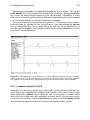
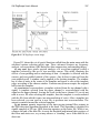
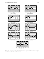
Appendix D
UW DigiScope User’s Manual
Willis J. Tompkins and Annie Foong
UW DigiScope is a program that gives the user a range of basic functions typical
of a digital oscilloscope. Included are such features as data acquisition and storage,
sensitivity adjustment controls, and measurement of waveforms. More important,
this program is also a digital signal processing package with a comprehensive set
of built-in functions that include the FFT and filter design tools. For filter design,
pole-zero plots assist the user in the design process. A set of special advanced
functions is also included for QRS detection, signal compression, and waveform
generation. Here we concentrate on acquainting you with the general functions of
UW DigiScope and its basic commands. Before you can use UW DigiScope, you
need to install it on your hard disk drive using the INSTALL program. See the directions on the DigiScope floppy disk. Also be sure to read the README.DOC file on
the disk for additional information about DigiScope that is not included in this
book.
D.1 GETTING AROUND IN UW DIGISCOPE
To run the program, go to the DIGSCOPE directory and type SCOPE. Throughout
this appendix, the words SCOPE, DigiScope, and UW DigiScope are used interchangeably.
D.1.1 Main Display Screen
Figure D.1 shows the main display screen of SCOPE. There is a menu on the left
of the screen and a command line window at the bottom. There are two display
channels. The one with the dashed box around it is called the active channel, which
can be selected with the (A)ctive Ch menu command. Operations generally
manipulate the data in the active channel. The screen shows an ECG read from a
disk file displayed in the top channel and the results of processing the ECG with a
derivative algorithm in the bottom (i.e., active) channel.
332
UW DigiScope User’s Manual
333
Maneuvering in SCOPE is accomplished through the use of menus. The UP and
DOWN ARROWS move the selection box up and down a menu list. Hitting the RETURN
key selects the menu function chosen by the selection box. Alternately, a menu
item can be selected by striking the key indicated in parenthesis for each command
(e.g., key F immediately executes the (F)ilters command).
An e(X)it from the current menu to its parent (i.e., the previous menu) can be
achieved either by placing the box on the e(X)it item and striking the RETURN
key, by hitting the X key, or by simply hitting the ESC key. In fact the ESC key is
used throughout SCOPE to exit from the current action, and the RETURN key is used
to execute a selected function.
Figure D.1 UW DigiScope’s main display screen. The dashed box indicates the active channel.
In this case, the ECG in the top channel was read from a disk file, then a derivative algorithm
was applied to processed the ECG and produce the waveform in the bottom (active) channel.
D.1.2 Communicating with SCOPE
Sometimes it is necessary for the user to enter data via the keyboard. Such data entry is done in the command line window at the bottom of the screen. Entry of data
either ends with a RETURN, upon which the data are accepted, or an ESC which
allows the user to quit data entry and make an escape back to the previous screen.
Correction can be done with the BACKSPACE key prior to hitting RETURN. SCOPE
also provides information to the user via short text displays in this window.
334
Biomedical Digital Signal Processing
D.2 OVERVIEW OF FUNCTIONS
Figure D.2 shows how main menu functions branch to other menus. Command
f(I)le permits reading or writing disk data files. Function real (T)ime lets you
select the source of sampled data to be either from a disk file or, if the computer
has the proper hardware installed, from an external Motorola 68HC11 microcontroller card or an internal Real Time Devices signal conversion card.
Function (L)imits lets you choose whether SCOPE functions operate on the
whole file or just the portion of the file that is displayed. The default limits at startup are the 512 data points from the file seen on the display. The maximal file size
is 5,120 sampled data points. When you write a file to disk using the f(I)le
(W)rite command, you are asked if you want to write only the data on the display
(512 points) or the whole file. With the scr(O)ll function, you can scroll through
a file using the arrow keys and select which of the file’s 512 data points appear on
the display. (C)opy performs a copy of one display channel to the other.
Figure D.2 Branches to submenus from the main menu.
UW DigiScope User’s Manual
335
Figure D.3 Filter design menus.
To adjust the amplitude of the active channel, select (Y) Sens and increase or
decrease the sensitivity of the channel by a factor of two each time you strike the
up or down arrow on the keyboard. This function operates like the sensitivity control on an oscilloscope. (M)easure superimposes two cursors on the waveform in
the active channel that you can move with the arrow keys. At the bottom of the
display, a window shows the time and amplitude values of the cursors.
Command stat(U)s provides a summary screen of information about the characteristics of the current data display. This information is recorded in the header of
a data file when it is written to disk.
Function (P)wr Spect computes and displays the power spectrum of a signal.
A (H)elp function briefly explains each of the commands. Selecting to e(X)it
from this main menu returns you to DOS. Choosing e(X)it on any submenu
returns you to the previously displayed menu.
Figure D.3 shows menus for performing filter design that branch from the
(F)ilters command in the main menu. Any filter designed with these tools can
be saved in a disk file and used to process signals. Tools are provided for designing
336
Biomedical Digital Signal Processing
the three filter classes, FIR, IIR, and integer-coefficient filters. (F)IR and (I)IR
each provide four design techniques, and I(N)teger fully supports development
of this special class of filter. The most recently designed filter is saved in memory
so that selecting (R)un filter executes the filter process on the waveform in the
active window. (L)oad filter loads and runs a previously designed filter that
was saved on disk.
Figure D.4 shows the filter design window for a two-pole IIR filter. In this case,
we first selected bandpass filter from a submenu and specified the radius and angle
for placement of the poles. The SCOPE program then displayed the pole-zero plot,
response to a unit impulse, magnitude and phase responses, and the difference
equation for implementing the filter (not shown). By choosing e(X)it or by
hitting ESC, we can go back to the previous screen (see Figure D.3) and
immediately execute (R)un filter to see the effect of this filter on a signal.
Note that the magnitude response is adjusted to 0 dB, and the gain of the filter is
reported. High-gain filters or cascades of several filters (e.g., running the same filter more than once or a sequence of filters on the same signal data) may cause integer overflows of the signal data. These usually appear as discontinuities in the output waveforms and are due to the fact that the internal representation of signal data
is 16-bit integers (i.e., values of approximately ±32,000). Thus, for example, if you
have a 12-bit data file (i.e., values of approximately ±2,000) and you pass these
data through a filter or cascade of filters with an overall gain of 40 dB (i.e., an
amplitude scaling by a factor of 100), you produce numbers in the range of
±200,000. This will cause an arithmetic overflow of the 16-bit representation and
will give an erroneous output waveform. To prevent this problem, run the special
all-pass filter called atten40.fil that does 40-dB attenuation before you pass the signal through a high-gain filter. The disadvantage of this operation is that signal bitresolution is sacrificed since the original signal data points will be divided by a
factor of 100 by this operation bringing a range of ±2,000 to ±20 and discarding
the least-significant bits.
UW DigiScope User’s Manual
337
Figure D.4 UW DigiScope screen image.
Figure D.5 shows the set of special functions called from the main menu with the
advanced options selection ad(V) Ops. These advanced features are frequency
analysis, crosscorrelation, QRS detection, data compression, and sampling theory.
(F)req anal does power spectral analysis of a waveform segment (called a
template) selected by the use of two movable cursors. This utility illustrates the
effects of zero-padding and/or windowing of data. A template is selected with the
cursors, and zero-padded outside of the cursors. Any dc-bias is removed from the
zero-padded result. A window can be applied to the existing template. The window
has a value of unity at the center of the template and tapers to zero at the template
edges according to the chosen window. Function re(S)tore recopies the original
buffer into the template.
(C)orrelation crosscorrelates a template selected from the top channel with a
signal. A template selected from the upper channel is crosscorrelated with the
signal on the upper channel, leaving the result in the lower channel. If you do not
read in a new file after selecting the template, then the template is crosscorrelated
with the file from which it came (an autocorrelation of sorts). After a template has
been selected, you can read in a new file to perform true crosscorrelation. The
output is centered around the selected template.
(Q)RS detect permits inspection of the time-varying internal filter outputs in
the QRS detection algorithm described in the book. This algorithm is designed for
signals sampled at 200 sps. QRS detection operates on the entire file. When it encounters the end of the data file, it resets the threshold and internal data registers of
the filters and starts over, so you may observe a “standing” wave if the data file is a
short one.
338
Biomedical Digital Signal Processing
Figure D.5 Advanced options menus.
Function c(O)mpress provides the option to do data compression of a waveform
using the turning point, AZTEC, Fan, and Huffman coding algorithms. The data
reduction techniques compute approximations to the data in the upper channel. The
UW DigiScope User’s Manual
339
algorithms operate only on the displayed data. The Turning Point algorithm reduces the number of data points by a factor of two, keeping critical points. The
FAN and AZTEC algorithms require a threshold, which determines a trade-off
between data reduction and distortion. The user is prompted to enter a value for the
threshold, preferably a fraction of the data range (which is displayed). Huffman
coding is a lossless algorithm that creates a lookup coding table based on frequency of occurrence of data values. A lookup table must be computed by (M)ake
before the data can be compressed by (R)un. (R)un actually compresses then decompresses the data and displays the data reduction ratio. When making the table,
first differencing can be used, which generally reduces the range of the data and
improves data reduction. If the data range is too great when executing (M)ake , the
range of the lookup table will be truncated to 8 bits, and values outside this range
will be placed in the infrequent set and prefixed, so data reduction will be poor.
The best thing to do in this case is to attenuate the data to a lower range (with a filter like atten40.fil) and then repeat the process.
(S)ample facilitates study of the sampling process by providing the ability to
sample waveforms at different rates and reconstruct the waveforms using three different techniques. This module uses one of three waveforms which it generates internally, so you cannot use this module to subsample existing data. The data is
generated at 5,000 sps, and you may choose a sampling rate from 1 to 2,500 sps at
which to subsample. When you take the power spectrum of data that has been
sampled (but not reconstructed), the program creates a temporary buffer filled with
512 points of the original waveform sampled at the specified rate. In other words,
even though the displayed data is shown with the intersample spaces, the power
spectrum is not computed based on the displayed data (and the 5,000 sps rate) but
rather with the data that would have been created by sampling the analog waveform at the specified sample rate. The reason for this is to illustrate a frequency
domain representation based on the specified sampling rate, and not the more
complicated power spectrum that would result from computing the FFT of the actual displayed data.
Function (A)daptive demonstrates the basic principles of adaptive filtering,
and a(V)erage illustrates the technique of time epoch signal averaging.
Figure D.6 shows the GENWAVE function that provides a waveform generator.
Signals with controlled levels of ran(D)om and 60-H(Z) noise can be synthesized
for testing filter designs. In addition to (S)ine, (T)riangle, and s(Q)uare
waves, ECGs and other repetitive template-based waveforms can be generated with
the t(E)mplate command. Figure D.7 shows two signals synthesized using this
function. Figure D.8 shows the nine different templates that are provided for
synthesizing normal and abnormal ECG signals. For more details about the
GENWAVE function, see Appendix E.
340
Biomedical Digital Signal Processing
Figure D.6 Waveform generation.
(a)
(b)
Figure D.7 Waveforms generated using (G)enwave. (a) Two-Hz sine wave with 20% random
noise. (b) ECG based on ECG WAVE 1 with 5% 60-Hz noise.
341
0.8
0.6
0.6
0.4
0.4
Amplitude (mV)
0.8
0.2
0
-0.2
0.2
0
-0.2
-0.4
-0.4
-0.6
-0.6
-0.8
0
Amplitude (mV)
UW DigiScope User’s Manual
0.1
0.2
0.3
0.4
-0.8
0.5
0
0.1
0.2
Time (s)
0.6
0.4
0.4
Amplitude (mV)
0.6
-0.2
0.2
0
-0.2
-0.4
-0.4
-0.6
-0.6
-0.8
0
0.1
0.2
0.3
0.4
-0.8
0.5
0
0.1
0.2
Time (s)
0.6
0.4
0.4
Amplitude (mV)
0.6
0.2
0
-0.2
-0.4
-0.4
-0.6
-0.6
-0.8
0
0.1
0.2
0.3
0.4
-0.8
0.5
0
0.1
0.2
Time (s)
0.6
0.4
0.4
Amplitude (mV)
0.6
0.2
0
-0.2
-0.4
-0.4
-0.6
-0.6
-0.8
0
0.1
0.2
0.5
0.4
0.5
ECG WAVE 6
0.8
-0.2
0.4
Amplitude (mV)
ECG WAVE 5
0
0.3
Time (s)
0.8
0.2
0.5
ECG WAVE 4
0.8
-0.2
0.4
Amplitude (mV)
ECG WAVE 3
0
0.3
Time (s)
0.8
0.2
0.5
ECG WAVE 2
0.8
0
0.4
Amplitude (mV)
ECG WAVE 1
0.8
0.2
0.3
Time (s)
0.3
0.4
-0.8
0.5
0
0.1
Time (s)
0.2
0.3
Time (s)
ECG WAVE 7
ECG WAVE 8
0.8
0.6
Amplitude (mV)
0.4
0.2
0
-0.2
-0.4
-0.6
-0.8
0
0.1
0.2
0.3
0.4
0.5
Time (s)
ECG WAVE 9
Figure D.8 Templates used by the GENWAVE function to generate ECG waveforms. Template
ECG WAVE 1 is normal, the rest are abnormal.