Download 0 - Ideals

S
I L L I NOI
0
UNIVERSITY OF ILLINOIS AT URBANA-CHAMPAIGN
PRODUCTION NOTE
University of Illinois at
Urbana-Champaign Library
Large-scale Digitization Project, 2007.
ILLINOIS
_.Ar'
•,•NATTTRA.
/--% mi
I 'Mr--IL 0 IL1 2ISL
HISTORV
0 MMLa
mma k-T0 14L
SURVEY
Manual for the District Fisheries Analysis
System (FAS): A Package for Fisheries
Management and Research
Part 2: Creel Survey Data Base
Aquatic Biology Section
Technical Report
Peter B. Bayley and Douglas J. Austen
Mark Thompson and Alan Citterman, Programmers
Aquatic Biology Technical Report 87/12
1%
Illinois Natural History Survey
Aquatic Biology Section Technical Report 87/12
MANUAL FOR THE DISTRICT
FISHERIES ANALYSIS SYSTEM (FAS):
A PACKAGE FOR FISHERIES
MANAGEMENT AND RESEARCH
Part 2: Creel Survey Data Base
Peter B. Bayley and Douglas J. Austen
Mark Thompson and Alan Citterman, Programmers
Peter B. Bayley, PrincipalAquatic Biology Section
estigator
Robert W. Gorden, Head
Aquatic Biology Section
September 1987
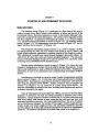
SUMMARY OF PROJECT
The major emphasis of this project was in the design and implementation of a
fisheries data base, the Fisheries Analysis System (FAS), that would provide
information for managers and researchers on a long-term basis. The secondary, but
no less important, emphasis was to interpret and analyze FAS data at the District and
State levels.
An overview of FAS is presented in Aquatic Biology Technical Report 87/10.
A description of the fish population survey data processing in the DISTRICT FAS part
of the system is described in the form of a manual in Aquatic Biology Technical
Report 87/11 which results from part of the work required under Jobs 101.1 and
101.3. Creel Survey data processing is described in Aquatic Biology Technical
Report 87/12 and completes the requirements under Jobs 101.1 and 101.3. The
statewide data base, STATE FAS, is described along with uploading and
downloading procedures in Aquatic Biology Technical Report 87/13 (Jobs 101.4
and 101.5). Technical Report 87/14 presents an analysis of efficiencies of gears
used in generating most of the data in FAS and an analysis of standard parameters
for condition factors, resulting from requirements under Jobs 101.2 and 101.6.
This technical report is part of the final report of Project F-46-R, Comparative Analysis of
Fish Communities in Impoundments, which was conducted under a memorandum of
understanding between the Illinois Department of Conservation and the Board of
Trustees of the University of Illinois. The actual work was performed by the Illinois Natural
History Survey, a division of the Department of Energy and Natural Resources. The
project was supported through Federal Aid in Sport Fish Restoration by the U.S. Fish
and Wildlife Service, the Illinois Department of Conservation, and the Illinois Natural
History Survey. The form, content, and data interpretation are the responsibility of the
University of Illinois and the Illinois Natural History Survey, and not that of the Illinois
Department of Conservation.
PREFACE
The data-base and programs of CREEL have been developed as part of the
District Fisheries Analysis System (DISTRICT FAS) to accommodate the typical
recreational fishery survey conducted by many state natural resource agencies.
CREEL allows survey design, data input, storage, and calculation of a variety of
important statistics that managers require. As a part of the FAS system, CREEL
runs on an Apple //e microcomputer and uses General Managerm as the data-base
management system. All interface programs are written in Applesoft BASIC Tm and
have been designed to be easily used and are, for the most part, interactive with the
user.
ACKNOWLEDGMENTS
Jana Waite is thanked for her excellent redactional work.
TABLE OF CONTENTS
Page
Chapter
1
Starting Up and Permanent Data Entry
1-1
Basic Information
Materials Required
Start Up
Permanent Data Entry
Supplemental Question Editing
1-1
1-8
1-8
1-8
1-9
2
Strata Entry
2-1
3
Data Entry
3-1
4
Data Analysis - Grouping
4-1
General Information
GROUPING
4-1
4-2
Appendix
A
Statistical Methods for Creel Programs
A-1
Chapter 1
STARTING UP AND PERMANENT DATA ENTRY
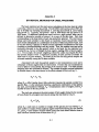
Basic Information
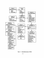
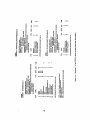
The data-base design (Figure 1-1) is analogous to a flow chart of the steps to
conduct a creel survey and to obtain valid estimates of effort and harvest of the
recreational fishery. Each box represents a screen in the General Manager m data
base and is composed of related information. The screens can be logically divided
into five categories: (1) permanent information in screens 1, 2, 3, and 13 (Figure
1-2); (2) stratum design information in screen 4 (Figure 1-3); (3) sampling dates in
screen 5 (Figure 1-3); (4) instantaneous count data in screen 6 (Figure 1-3); and (5)
angler interview data in screens 7-12 (Figure 1-4).
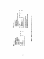
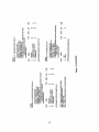
The permanent information stored in screens 1, 2, 3, and 13 (Figure 1-2) does
not change during the creel year and includes such items as region, district, and
length-weight regression parameters to estimate weights of fish caught by anglers.
This information is entered once using General Manager's data-entry routine. As
with DOC9, all other data entry uses custom-designed programs. The data-entry
routine of General Manager should not be used for screens 4-12. However, when
correcting errors, BROWSE/UPDATE should be used.
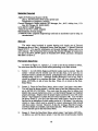
Stratum design information, stored in screen 4 (Figure 1-3), allows the creel
manager to designate how the lake will be divided by area and time periods. In most
lakes, some stratification is used to efficiently allocate survey effort. Stratification
information is used in the calculations and is entered using the program STRATA
ENTRY.
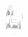
Instantaneous count data are stored in screen 6 under the appropriate sampling
date in screen 5 (Figure 1-3); it is the basic unit of measurement used to calculate
fishing effort. Instantaneous count data are entered in conjunction with interview
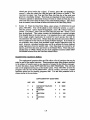
data using the program DATA ENTRY. Finally, interview data are entered into
screens 7-12 (Figure 1-4), one interview at a time, using DATA ENTRY. All
interview information is entered at one time, including such supplemental questions
as distance traveled by the angler.
Once all information has been entered into CREEL, you may use several output
programs to summarize the data and obtain estimates of pertinent creel survey
parameters. Output programs currently available are (1) an effort table that gives
total hours fished, total number of trips, hours per trip, and hours per acre, with
associated confidence intervals; (2) a catch table that shows, for up to 10 species
and a miscellaneous category, the number of fish caught, number caught per hour,
weight caught, and weight caught per hour, with associated confidence intervals;
and (3) a generic set of tables that calculates frequencies of response to supplemental
questions. The statistical calculations to produce these values are in Appendix A.
1-1
Screen 1
REGION/DISTRICT
Lake*
Acreage
Shoreline length
Mean depth
Region*
District*
District biologist
Screen 13
SPECIES
i
Screen 9
RELEASED
LENGTH-FREQUENCY
Screen 7
INTERVIEW DATA
4-
Species*
Length group (cm)*
Sample frequency
Total frequency
Screen 3
START OF
CREEL YEAR
Year *
First date*
Day of week
Dates of holidays
Species*
Length to weight
conversion parameters
Screen 8
HARVESTED
LENGTH-FREQUENCY
4Wm
n
Screen 2
LAKE
-
I
Species*
Length group (cm)*
Sample frequency
Total frequency
Interview number*
Time
Boat/shore
Complete/incomplete
Party size
Species sought
Hours fished
Zero catch (Y/N)
Stratum*
Section*
First date*
Last date*
Sampled days/weeks
Fishable hours/days
Creeled hours/day
Daily sampling periods
Section description
Acreage
Screen 5
INTERVIEW DATE
1 1Julian day *
I-14
Weekday/holiday-weekend *
Date
Screen 6
INSTANTANEOUS
COUNT DATA
Time*
Number of boats
Number of boat anglers
Number of shore anglers
Air temperature
Water temperature
Secchi disk
Wind condition
Weather condition
Water level
Screen 10
HARVESTED
GROUP DATA
Screen 4
STRATUM DESIGN
4-"
Species*
Lower total length
Upper total length
Frequency
Screen 11
RELEASED
GROUP DATA
Species*
Lower total length
Upper total length
Frequency
Figure 1-1. Hierarchical structure of CREEL.
1-2
00T-
,,
0
i
INI'-
93
>
0
0
w
Cd
i0
C#)
0
o.
z ac4 gjI
Cc
-cr
•c
ý.c ZUJ
01
w
W•
uc
~
0
mp x
rMCO
2^
2
•G 32 .0
0
cc 0
CC
cc
0m
w
5:3CQ
o2 cc
ccy)
Y
C
jw
X
ww
I
cc
.1
Ill
cc
^UJ
0.ciz~
C6
-i
C.
0
c'5
JN
C,,.
coi
ULL>
N
LL
C,
co
ci:
z
co
vNCO
DcaCO8
O8 0
jD^
5Qs0<CO
VWD
0L
5z 0.
j
r
w
w0
w0
Z
C
w
Ncc
w0cc
1-3
0..
C
Ci)
id
01 O
w
L:
0
Li.
0
I-
a:
I-
CV)
w
rU-u
liUil
w
COj.Cvw, ZXOb
0 L
:oo -U
0
0.
ci
W X3:
CU)
0 0w
w-C
z
Iwa
^N{3oo0.
0o
S2w
0
I(M
o
o
C~J
cc fr) «*^^^* ^^*
ga:CM
CM C,8
w
=3
._•
u_
LL
0
LL.
I I
t
u
Co
w
cc
id
CO
0
wa:
zw
-J
a:
w
a:
xLU
0
w
0
cc
w C
-w
0-
.
S-M
Nov
wo0
10
14
a
Nm
CCJ D
LiZ~
W
0000.-
w
cc
LU
CMf
w 2
w
T-00
C C0
CC
w0
oa
z GI
^
afn 0-To
UM/
3ii8w
CQ~ w-c
0
w
w
C/)
1
0
w
N
z
w
w
o
>.
•0w
0
w
w
-J
<
r
>.W
W
C1
0
12
00
Zss
(0
w
cc
w
'-M.
w
do
o~o 0 ^0
LU
<Qj
CO
w
wS
U..U.
ooooU->>>>>>WWWA*A
L. L. L.
§cra
U.
No
" O 'w- of-.
rNmvOO»
C5~
qqi
U)
(0
w
a
V-"
0
LL
0
C
NM
D€D
c0
1
41
O)
9
1i
Go
0
>U. IL LI. LA.U. U. ).
-J
I-
41 w
8
0
0u•
0
0
0cra:
USLL,
(0
WHc
CO)
0
UL
w
M
<o
a a.
.^
z
ED
cc
cr.
wwC
§
Cl)
V-
SdW 0w
S
(
cc
W:x
0
/ U.
uwrr
co
0)
f*-
1-5
.w
%OM
NgS
^isi
LL.
000
000
C') CO)C') C')
6
OLI.
z
ocr
w
LL
I»>
>
Z
o
w
0»
jO)>
C
z
0
cc (L
eL
w wr
6u
-J5
w
IJW
C
0
s
U)o
w
CO)
zz
CO
c
wg~g!
z
zW 0
OnwO
CY
N
0
w0
Z
00,00 Opp
w
LI.
I
I0
2
0
CL
zL~
WCOI0..
0C
c
0
.1.
0
0
-
.<5
aNCb
U,
Lu
C)
LL0
Ir
0
0?
0000>WW>LL>W
C 4)
1-
0
Lw
a.
0"
i-0
-.
CO = 0
W2LL*
w
0
•i
U£
s
0
00 w
Lu
Z
UZ
ccWcX;
Id
Lu
SNC')1(O
tB0L00
1-6
F.
0.0.
C-C
-JZ
UJD
000
w
rc
5
0
cc
0L.
LU-
0
vw
0
cc C
5w0<
Lcr.
LL
>>> CM
a..»
0
a:
T-
0c
a
CCiFlcc
,-8 0
cc
cc
WW0
00
0
cc
0
ww
w cc
cco
x C.)0V- m
0 ZCC
0ý<8 ° g
a.Z
cc
0z
wccc=
ct
-i^
D0
0
.-
0
J
.-Jj
Oh< 2-L
0)
eo
wz
ZZ i
S*
•w--.|o
w0z5
V-IL
z
in
0
a-.
0o
cc.
0
gL
- 4t
0.
W
cc
cc
0L(icr
,
CM
00
C.
8-
co000
COCOC C
cco
0
I-
Q
CL ccc|
ooO
> >> Ch
LL
0
d
z
-J 0
0 PWw
Z CC
CO
-.J ,_j
0c-0s.2
!,-
cco
I-
ww
z
%
E
0
(W.
::}
* ou*
S CLo
O> -
cc
a.N0
0(0J
w
cc
cr.
1-7
wcc 3
WJCC
W*U
C*
CLU
-JD
Z
Apple //e Professional System (128 K)
plus C. Itoh Prowriter (8510 series) printer and
Graphicard (or Grappler+) interface
General Managermr Master diskette (PC Manager, Inc., 64 E. Ashley Ave., P.O.
Box 567, Driggs, ID 83422-0567)
DATA ENTRY: CREEL Diskette
TABULAR OUTPUT: CREEL Diskette
Blank diskettes for data storage
A RAMFACTOR', (Applied Engineering) card and an accelerator card or chip are
recommended.
Start Up
The major steps involved in system booting and simple use of General
Manager are given in Part 1: Biological Survey Data (see page 1-1, Special Technical
Report 87/11). For specific information on General Manager, please refer to its
user's manual. The instructions below assume that General Manager is booted, that
you are in the DATA ENTRY option of ACCESS DATA BASE, and that a formatted
data disk is in drive 2.
Permanent Data Entry
As shown in Figure 1-1, screens 1, 2, 3, and 13 are the top screens in CREEL.
You must enter data for the key fields before proceeding to the other screens.
1.
Screen 1: As with DOC9, Region and District codes must be entered. Data for
screen 1 should only be entered once for the data base, so be sure that no
duplicate screen 1 records are entered. If duplicates exist, delete the erroneous
records using <CTRL-D>. Although District Biologist is not a key field it
should be entered for a complete data base. Once you have entered the data,
press <RETURN> or <4> to save the data. Press <6c> to return to the Data
Entry Menu.
2.
Screen 2: From the Data Entry Menu, select screen 2 and press <RETURN>.
You will then be shown screen 1 with the next to last line indicating that you
are to ENTER KEY CRITERIA. You must enter the same data for region and
district that you just entered into screen 1 so that General Manager can establish
proper parentage. Simply enter the proper region and district (you will notice
that an = sign appears as a prefix for each entry) and press <t>. You will then
be shown screen 2; you are in the data entry mode (again, check the next to
last line for an indication of which mode you are in ). In screen 2, the only key
criteria is Lake, which must be entered to connect subsequent child records
with that screen 2 record. However, if data for Acreage, Shoreline Length,
and Mean Depth are available, enter those data also. When finished, press <4>
to save and then quit to the Data Entry Menu.
3.
Screen 3: From the Data Entry Menu, select screen 3 and press <RETURN>.
As before, you will be shown screen 1 but this time the previously entered
1-8
criteria are given (notice the = signs). If correct, press <#> and proceed to
screen 2; enter the criteria for Lake and press <t> to move to screen 3. The
two keys in screen 3 are Year and First Date (the first day of the creel year
given in a month/day format). These data are important for later calculations.
Consult a calendar to determine the day of week on which the first day ot the
creel year falls and to find the dates of the listed federal holidays. Once these
data are entered, save the data as before and return to the Data Entry Menu.
4.
Screen 13: From the Data Entry Menu, select screen 13 (SPECIES-13) and
press <RETURN>. You will be asked to enter criteria for screens 1, 2, and 3.
Data for screens 1 and 2 should be displayed; press <d> if these values are
correct. For screen 3, enter Lake and First Date and press <t>. Screen 13 will
then be displayed. This screen contains the information to convert weights
from lengths taken in the creel surveys. It is important that a and b parameters
from length-weight regressions be entered for each species that will be
encountered in the creel survey. Obtain these data from the most recent fishery
survey conducted on the lake by the district fisheries biologist. If such data are
not available, then values from standard length weight regressions may be
used; however, calculated weights may not be as accurate as those obtained
using regressions from the specific lake. Once these data are entered for all
species, quit from data entry and return to the Master Menu. From this point,
all data entry in CREEL should use one of the programs accessed under USER
PROGRAMS selected from the Data Base Master Menu.
Supplemental Questions Editing
The supplemental question editor and file refer to a list of questions that may be
asked as part of the angler interview. These questions range from distance traveled
to the amount of money spent to any question of interest to the fisheries manager.
To enter the editor, choose SUPP QUES ED from USER PROGRAMS. This will load
and run the program leaving you at the header screen. Press <RETURN> to have the
program read the file SUPPLEMENTARY, which contains previously created
questions stored on the working programs disk. You are then presented with a
screen similar to the one below.
SUPPLEMENTARY QUESTIONS
USE KEY
Y
A
N
B
N
C
N
D
#
PROMPT
DISTANCE TRAVELED
INMILES
QUESTION
#2
QUESTION
#3
QUESTION
#4
1-9
MIN
MAX
Y
0 9999
Y
0
100
Y
0
100
Y
0
100
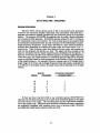
A maximum of eight questions may be stored in the program. The first
column, USE, indicates if the question will be used in the survey, If Y,the question
will be asked during data entry after fish length data are entered. If N,the question
is suppressed. The next column, KEY, is the data-base designator for the question
and is the key field used by General Manager to search for questions to be analyzed
in output tables. The PROMPT column is the two-line phrase shown on the screen
during data entry. If the question requires a numeric answer (e.g., distance in
miles), the # column should have a Y; if the answer is in alpha characters (e.g., yes
or no), N should be entered in this column. This designation provides error
checking during data entry. Alpha characters cannot be entered if a numeric answer
was specified. Similarly, MIN and MAX indicate the lower and upper ranges
accepted; values outside of the range will be rejected.
To edit the supplemental questions, press <RETURN> to move to the part that
needs to be changed. The arrow keys cannot be used to move backward; move to
the bottom using <RETURN> and then answer NO to the question IS THE DATA
CORRECT? This will put the cursor at the top of the screen and allow you to further
edit the supplemental questions.
1-10
Chapter 2
STRATA ENTRY
From Data Base Master Menu, select UTILITIES, and then from the Utilities
Menu select RUN USER PROGRAM. You will be asked if you want to use the
CREEL data base; answer YES (YES is the default and is selected by pressing
<RETURN>). You should now have to the User Programs Menu on the screen.
Select STRATA ENTRY and press <RETURN>. A title screen will appear; to continue
the program, press <RETURN>.
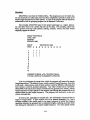
The STRATA ENTRY program will read the data in screens 1, 2, and 3 and ask
you to select a combination of criteria. Once you have selected the Region, District,
Lake, and Year, a SECTION DESCRIPTION screen which appear:
REGION 1 DISTRICT
LAKE TEST
YEAR 1987-1988
SECT ACREAGE
(1000)
DESCRIPTION
.......
0
.......
....
.............
... .....................
4
S.......
.......
...... ..................
........................
7
.......
........................
8
9
.......
.......
0.
........................
oo
..... ..............
2
10
...............................
ENTER ZERO ACRES TO DELETE SECTION
You may now designate subdivisions (sections of the lake) for spatial
stratification. Up to 10 sections are allowed; the acreage of each should be defined
as well as a brief description of the section. The sum of the section acreages must
equal the total lake acreage in screen 2, listed here under ACREAGE. These section
designations comprise the spatial component of the stratum (the temporal is
discussed below), which is used in creel survey design and in statistical estimates.
Later, calculations may be done by individual stratum, any combination of strata, or
the lake as a whole.
Once section descriptions are complete, you are shown the screen that permits
stratum designation. This rather complex screen is divided into several different
columns for each section of the lake. Each column has five components: the first
2-1
and last date of the period, the number of days sampled per week, the number of
fishable hours per day, and the number of hours creeled in a day. STRATA ENTRY
automatically places the first day of the creel year under the first period in section 1.
You are then asked to enter the last day of the period and the values for the three
additional parameters. The cursor then moves to the next period in that section and
the next date that needs to be accounted for in the stratum designation. This process
is continued until all periods are completed for the section. NOTE: Periods,
from first to last, must account for a complete year even if creel data
were not collected during a time period. If no activity occurs (e.g., if a
section of the lake is closed for duck hunting), enter the appropriate data and zeroes
for the sampled days per week, fishable hours per day, and creeled hours per day.
The editing mode in STRATA ENTRY is entered by pressing the <SPACE BAR>
several times over the field where dates are entered. The command area at the
bottom of the screen indicates the available options. The arrow keys move the
cursor and the current stratum available for editing is marked by an asterisk (*).
Entering an capital I (<I>) inserts an additional stratum immediately after the current
stratum, <D> deletes the current stratum, <C> copies the stratum immediately to the
left of the current stratum and writes the copy at the current stratum. If the current
stratum is the first in that section, <C> will copy the entire previous section into the
current section. Press <RETURN> to return to normal input mode.
To exit from stratum designation, get into edit mode and press <E> for exit.
The program will then check the stratum for missing days or improper days (e.g.,
too many days in a month). If an error is found, you will be sent back to the stratum
designation screen. When this screen is validated, you will be asked if you want a
printout of the strata, if you want to do more editing, and whether you want to enter
daily times for instantaneous counts. Once the stratum table is completed and saved,
you are asked if you want to complete times for day-periods and instantaneous
counts for screen 4 (at this time, it is informative to complete the daily times for the
instantaneous counts although it is not necessary).
The stratum design screen (Figure 1-3) appears as below:
STRATUM
SECTION
ACREAGE
Section Description...
PERIOD MM/DD - MM/DD
SAMPLED DAY/WK
FISHABLE HRS/DAY
CREELED HRS/DAY
START #1
COUNT #1
START #2
COUNT#2
START #3
COUNT#3
2-2
All information should be complete with the exception of the COUNT field,
which represent the starting times of the instantaneous count associated with each
period. Up to three periods are allowed but less than three can be used. However,
if less than three periods are used, the end time of the last period used must be
entered in the start time slot for the first unused period. Normally, one count is
made during each period and is started at a designated time. This information must
be entered for each stratum and is stored in screen 4. Now all the basic information
for the creel survey has been entered. Survey data are now entered using DATA
ENTRY.
2-3
Chapter 3
DATA ENTRY
The entry of survey data, instantaneous counts, and angler interviews is
accomplished by using the program DATA ENTRY. This program is accessed
through General Manager and the Main User Program Menu. You will be given a
heading screen indicating the name, date, and programmers; press <RETURN> to
continue. You are then asked if your measurements are in English or metric units.
If English units were used to measure fish, the program runs an algorithm that
converts the units, taken to the nearest 0.5-inch, into centimeter groups. When an
English measurement could correspond to two or more 1-cm groups, a random
number generator allocates that data to a single 1-cm group, taking into account the
probability assignments to alternative groups.
As with STRATA ENTRY, you proceed through the sequence of selecting
parentage for the data to be entered. The program asks you to select the region,
district, lake, year, and section and then to enter the date of the creel survey
information. The program checks the date against the appropriate stratum and
determines whether it is a weekend/holiday or weekday and brings up the first
screen for data entry, the instantaneous count information.
The format of the instantaneous count screen mimics the field data sheet and
permits convenient data entry directly from the data sheets. All information is
self-explanatory. Wind, sky, and water level descriptors are the first letter of the
word chosen as indicative of the conditions (e.g., L for light winds). Once complete
and you have answered YES to the question of whether the data are correct, the
information is saved as a record in screen 6. Another screen is brought up and you
can enter additional counts for the creel day. If you have no further data to enter,
press <ESC>.
Angler interview data are entered in four stages. The first stage is data on the
angler (e.g., time of interview, party size), the second and third stages accept
information on harvested and released fish, respectively, and the fourth on
supplemental questions (e.g., distance traveled). In the first stage, interview
number and time refer to the sequence of anglers interviewed in the creel day and the
actual time that the interview occurred. Boat or shore fishing is designated with a B
or S, and complete versus incomplete interviews with a C or I. Party size is the
number of anglers in the party, species sought is the standard three-letter code (or
ANY if there was no preference), and hours fished is the number of hours fished at
time of interview.
Data on all harvested fish are entered, one species at a time, for each line on the
screen. Slashes or commas separate individual fish measurements and hyphens
separate the lower and upper lengths of a group count. For group counts, the
number of fish in the group is requested. For example, if the angler caught four
largemouth bass of 36, 37, 39, and 42 cm, 10 bluegill ranging from 15 to 20 cm,
and one trophy-size bluegill of 24 cm, the data would be entered as follows:
3-1
INTERVIEW NO. 1 (PRESS ESC WHEN DONE)
HARVESTED
SPECIES LENGTHS
LMB
36/37/39/42...........
BLG
BLG
15-20 ..................... AMT 10
24
Group counts must be placed on a separate line from that of individual fish
lengths. Fish lengths separated by slashes or commas are assumed to be for single
fish. If more than one fish has the same length, enter them separately or use group
input. For example, if two LMB have lengths of 35 cm, enter as 35/35 (or 35,35) or
as a group with length range of 35-35 and an amount of 2. If there are too many
individual fish measurements to fit on one line, use the same species code and
continue entry on the next line. Similarly, if you fill the screen, save the current
screen by answering YES to the question of whether you have more harvested fish
data. This will refresh the screen and allow entry of additional data. To exit from
harvest data entry, press <ESC>. Individually measured, harvested fish are stored
as screen 8 records while group counts of harvested fish are stored as screen 10
records. Corresponding data for released fish are stored as screen 9 and 11 records,
respectively (Figures 1-1 and 1-4).
Data on released fish are entered using the same format as for harvested fish.
When completed with data entry, press <ESC> to quit. After all fish data are
entered, you are asked to enter data on designated supplemental questions. Once
this is done, data entry for the current interview is complete and you are ready for
the next angler interview. You may continue to enter data or press <ESC> to quit.
3-2
Chapter 4
DATA ANALYSIS - GROUPING
General Information
Because CREEL allows group counts of fish to be entered (with associated
minimum and maximum lengths) rather than only individually measured fish, a
program was needed to allocate grouped fish into centimeter groups in an equitable
manner. The program GROUPING accomplishes this by using a simple algorithm
and a random-number generator. GROUPING searches screens 10 and 11 for species
for which group counts were entered. For each of these species, the program finds
all individually measured fish from records in screens 8 or 9 and formulates a master
length-frequency distribution. Each master distribution is from either harvested or
released data, depending on whether the.group count was from screen 10 or 11,
respectively. Then the group count data, upper and lower range, and number are
read into the program one species at a time. The upper and lower lengths of the
range are compared with the master length-frequency distribution for that species. If
there are at least three fish for each centimeter group in the master length-frequency
within that range, the length frequency is considered good and the fish in the group
count are allocated based on direct proportions to the number of fish in that section
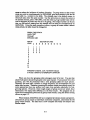
of the length frequency. For example, if there is a group count of 10 bluegill with a
length range of 15-20 cm and the length frequency from individually measured fish
is as follows in the middle column, the group count will be allocated as in the right
column:
ESTIMATED FREQUENCY
MASTER
LENGT
15
16
17
18
19
20
FREQUENCY
INGROUP COUNT
3
4
7
11
5
3
1
1
2
3
2
1
If there are fewer than three fish in any centimeter group, GROUPING first
allocates one fish from the group count to each of the centimeter groups at the upper
and lower limit of the range. The remaining fish are then distributed randomly
across the length range. Statistical errors involved with these allocation algorithms
are negligible compared with sampling errors due to between-angler variation,
providing that length ranges of group counts are small.
4-1
Grouping
GROUPING is run from the Utilities Menu. The program acts on the entire data
set and should be run after data entry has been completed to provide a good set of
master length frequencies for each species. A copy of the original data set should be
maintained so that the grouping program can be repeated if necessary.
Once loaded, GROUPING asks for the proper parentage (i.e., region, district,
etc.) and then shows you a screen that sets up the strata. For example, a lake with
three sections and four time periods (spring, summer, winter, and fall) would
originally appear as follows:
GROUP THE STRATA
LAKE=TEST
YEAR=87
SPECIES: LMB
PER OF
YEAR 1
SECTION OF LAKE
a
O Q Q
Q
2
1
1
1
1
2
1
1
1
3
1
1
1
4
1
1
1
OQQ
5
6
7
8
9
10
11
12
ARROWS TO MOVE, <CR> TO ENTER VALUE,
G TO GO. ENTER Q TO UNGROUP A STRATUM
You may designate the strata from which the program will search for master
length frequencies. The default shown would construct length frequency from data
in all strata. Alternatively, each of these numbers could be different, indicating that
each stratum would be grouped separately. Any other combin ation is possible.
GROUPING will search each stratum individually for grouped fish, create a master
length frequency for each species in that stratum, and allocate the grouped fish in the
stratum based on that length frequency. The program will then move to the next
stratum automatically.
In some cases, especially for smaller fish, few individually measured fish are
found in single strata. If each stratum was to be treated separately (i.e., had a
different number), this would result in too many instances in which the program
randomly allocates the grouped fish to centimeter lengths, reducing accuracy rather
than basing the allocation on a master length frequency. You must group similar
4-2
strata to reduce the incidence of random allocation. To group strata so that several
strata are acted on simultaneously by GROUPING, give each stratum in the set the
same label (i.e., number) in the table. The ultimate case is the default screen, in
which all strata have the same number. Use the arrow keys to move the cursor to
the desired stratum, press <RETURN>, and then enter a group number that will be
used to designate all strata that will be in the group. This unique number can be any
that you like and all strata given this number will be acted on simultaneously by
GROUPING. Using the same example as above, to group all strata within a season
(time period), the table should be changed to:
GROUP THE STRATA
LAKE=TEST
YEAR=87
SPECIES: LMB
PER OF
SECTION OF LAKE
YEAR
1
2
3
4
5
6
7
8
9
10
11
12
a 3.
1
2
3
4
1
2
3
4
Q
0
Q
0
QQ
1
2
3
4
ARROWS TO MOVE, <CR> TO ENTER VALUE,
G TO GO. ENTER Q TO UNGROUP ASTRATUM
When you have the grouping table arranged, enter G for 'go.' You are then
asked if all species should be grouped in the same manner. If you answer NO to this
question, you will be presented with a new grouping table for each species.
Generally for most lakes, variation in length frequency will be dependent on time
rather than location. Therefore, grouping all sections within time periods would be
more appropriate than one section over many time periods, especially for fastgrowing species. However, when length ranges of group counts are small, these
refinements will make little difference to the final results. The program has an
option that automatically processes all group count records, using the default setting
shown on page 4-2.
When finished, GROUPING will have completed all chosen stratum and species,
allocated all group counts to individual centimeter categories, and erased the old
group count records. The data base is now complete and ready for analysis and
tabular output.
4-3
Chapter 5
DATA OUTPUT
Output options were designed to provide basic summary data for management
decisions and breakdowns of strata and substrata for research into methods of
improving the survey design. The statistical approach is described in Appendix A.
1.
Run the program STATCALC, which calculates the means, variances, and
sample sizes for each substratum and group of strata and stores them in text
files. These interim text files can be stored on a DOS 3.3 diskette or on the
RAMFACTOR card. Groups of strata to be included subsequently in a stratified
analysis (Appendix A) are selected by the same process as described in Chapter
4 for length-group allocation. The simplest choice is one group for the entire
impoundment and year.
2.
You are then asked to select species for analysis. The contents of a file
containing the latest species list are read. This list can be edited and is
automatically saved in the same file. Up to 10 species are allowed. Two
additional categories, all species combined and miscellaneous species (all
species except those selected), are automatically included in the calculations for
a maximum of 12 taxa.
3.
A series of options in STATCALC allows you to coalesce substrata across strata
within each group. Suppose that the print-out of summary statistics (see 4)
during a previous run indicated that the number of samples during some
combinations of day-period and weekday/weekend are very low or nonexistent
in a stratum, you can choose to coalesce the data across all strata within each
group. This maintains the substrata, which we believe explain much of the
variance. Groups consisting of a single stratum will be unchanged. Another
alternative allows coalescing across substrata (e.g., pooling data from day
periods).
4.
The option: DO YOU WANT TO PRINT OUT SUMMARY STATISTICS BY
SUBSTRATUM (Y/N) is useful in deciding whether to coalesce strata in a rerun
and in improving sampling design. If this option is selected, you are asked to
choose between harvest and catch and between numbers or weights and desired
taxa. The output is too voluminous for all combinations, but all 12 taxa can be
printed. Visual comparisons of sample sizes, means, or variances will reveal
any shortcomings with any combination. The print-out contains one line for
each substratum and codes for day-period, weekday/weekend, boat/shore/
combined, stratum, section, year-period; data for days sampled, days possible,
mean daily effort with variance; and mean CPUE with variance and mean catch
(or harvest) with variance data for each taxa.
5.
One text file for the statistics for each group of strata is saved by STATCALC. If
all taxa and no coalesced data were selected, one group containing one strata
would occupy about 20 Kbytes of disk space. More disks can be used if
necessary. Speed and capacity are increased using the RAMFACTOR card
5-1
option. Normally, one group containing all the strata will be selected for
output of statistics from the entire impoundment during 1 year, with or without
coalesced strata.
6.
Exit to the General Manager menu or proceed directly to the program FINAL,
which combines the strata and substrata within each group selected, using the
text files output by STATCALC and the calculations in Appendix A. FINAL
asks you to select a group, then a confidence level of a = 0.05 or 0.10. The
following menu is then shown:
1. PRINT EFFORT TABLE
2. PRINT CATCH/HARVEST TABLE
3. CHOOSE NEW GROUP
4. CHOOSE NEW CONFIDENCE INTERVAL
5. EXIT
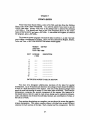
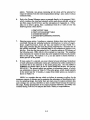
7.
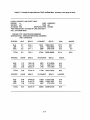
Selecting menu option 1 produces a summary broken down into boat/shore/
combined fishing and weekday/weekend combinations in terms of anglerhours, angler-hours/acre, hours per trip, and number of trips (Table 5-1).
Each page contains data for each day-period, followed by a summary for all
day-periods combined. The combined data for all substrata are shown in the
last row. Note that the time period is for 12 months, ending on 29 February of
the following year, 1988, which in this example is a leap year. The sampling
ratio represents the number of dates that were sampled divided by all possible
dates in the group. For options 1 or 2, you are asked to choose between a
screen preview or the printer.
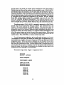
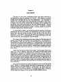
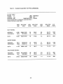
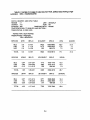
8.
If menu option 2 is selected, you must choose between printing a breakdown
of each substratum combination (strata are combined, but unless coalesced are
accounted for in the analysis) or the entire group only: DO YOU WANT A
SUMMARY OF GROUP ONLY (G) OR OF EACH SUBSTRATUM (INC. THE ENTIRE
GROUP(S)? The second option can produce a voluminous output, of which
one substratum is shown in Table 5-2. The entire group, which would typically
be the entire lake for 12 months, is output from either option; an example is
shown in Table 5-3.
CREEL is a complex data set which we believe is necessary to allow for the
numerous sources of variance and to maximize the advantages of stratification built
into the sampling design. Inevitably there are many ways to output summary data
and to design new surveys; therefore we have avoided 'black-boxing' the output at
this stage. Further development of the output programs STATCALC and FINAL will
continue during F-69-R as we analyze data from a variety of impoundments.
5-2
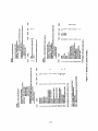
Table 5-1. Example of output effort from FINAL (artificial data).
EFFORT TABLE
LAKE :=GANDALF
:=1
REGION
YEAR :=87
DISTRICT :=01
SAMPLING RATIO :=29/365
ACREAGE :305
TIME PERIOD 03/01 TO 02/29 OF LAKE SECTION 1
TIME INTERVAL 2 (1000-1600)
-------
------
-
-
HRS/
ACRE
95% CONF
INTVL
ANGL
HRS
-
-
-
-
-
-
-
-
95% CONF
INTVL
HRS/
TRIP
95% CONF
INTVL
-
-
-
-
# OF
TRIPS
-
--
BOAT FISHING:
WEEKDAY:
WEEKEND/H:
11532
3513
10899-12165
3210-3816
38
12
36-40
11-13
6.8
9.1
6.4-7.2
8.9-9.2
1698
386
BOTH:
15045
14223-15744
49
47-52
7.2
6.8-7.6
2084
8211
2928
8003-8419
2725-3131
27
10
26-28
9-10
7.1
9.3
6.9-7.3
9.2-9.4
1156
315
11139
10869-11409
37
36-37
7.6
7.4-7.8
1471
SHORE FISHING:
WEEKDAY:
WEEKEND/H:
BOTH:
BOAT/SHORE FISHING:
WEEKDAY:
WEEKEND/H:
19743
6441
19114-20372
6029-6853
65
21
63-67
20-22
6.9
9.2
6.7-7.1
9.1-9.3
2861
700
BOTH:
26184
25302-27066
86
83-89
7.4
7.2-7.6
3561
5-3
Table 5-2. Example of one page of output data from FINAL (artificial data) showing a single
substratum. MSC - miscellaneous fish.
CATCH, HARVEST, AND CPUE TABLE
LAKE :=GANDALF
:=1
REGION
YEAR :=87
DISTRICT :=01
SAMPLING RATIO :=20/365
ACREAGE :305
TIME PERIOD 03/01 TO 02/29 OF LAKE SECTION 1
TIME INTERVAL 2 (1000-1600)
FISHING TYPE: BOAT FISHING
WEEKDAY/END: WEEKDAY
FISH: HARVESTED
#/HR
95% Cl
BLG
LMB
MSC
3.5
1.2
0.6
3.3-3.7
1.1-1.3
0.4-0.8
TOTAL
5.3
SPECIES
SPECIES
KG/HR
95% Cl
#/HA
#/ACRE
6420
2175
925
6180-6660
2020-2330
880-970
52.0
17.6
7.5
21.0
7.1
3.0
4.9-5.7
9520
9130-9910
77.1
31.2
95% Cl
KG CAUGHT
95% Cl
#CAUGHT
KG/HA
BLG
LMB
MSC
0.94
0.88
0.13
0.91-0.97
0.84-0.92
0.11-0.15
1710
1592
233
1675-1745
1570-1614
226-240
13.9
12.9
1.9
TOTAL
1.95
1.89-2.01
3435
3392-3478
28.7
SPECIES
LB/HR
95% CI
BLG
LMB
MSC
2.07
1.94
0.29
TOTAL
4.30
LB CAUGHT
95% CI
LB/ACRE
2.01-2.14
1.85-2.03
0.24-0.33
3771
3510
514
3693-3848
3462-3559
498-529
12.4
11.5
1.7
4.17-4.43
7795
7479-7669
25.6
5-4
Table 5-3. Example of output data from FINAL (artificial data): summary of one group of strata.
CATCH, HARVEST, AND CPUE TABLE
LAKE :=GANDALF
REGION
:=1
YEAR :=87
DISTRICT :=01
SAMPLING RATIO :=49/365
ACREAGE :305
TIME PERIOD 03/01 TO 02/29 OF LAKE SECTION 1
FULL DAY (0600-2200)
FISHING TYPE: BOAT/SHORE COMBINED
WEEKDAY/END: WEEKDAY/WEEKEND COMBINED
FISH: HARVESTED
#/HR
95% Cl
# CAUGHT
BLG
LMB
MSC
5.7
1.9
0.9
5.3-6.1
1.7-2.1
0.7-1.1
18211
6125
2988
16909-19513
5320-6930
2870-3106
147.5
49.6
24.2
59.7
20.1
9.8
TOTAL
8.5
7.9-9.1
27324
25992-28656
221.4
89.6
KG/HR
95% Cl
SPECIES
SPECIES
95% Cl
KG CAUGHT
95% Cl
#/HA
KG/HA
BLG
LMB
MSC
1.74
1.56
0.63
1.56-1.92
1.44-1.68
0.52-0.74
5231
4716
1799
5112-5320
4650-4774
1701-1897
42.4
38.2
14.6
TOTAL
3.93
3.72-4.14
11746
10231-13213
95.2
LB/HR
95% Cl
BLG
LMB
MSC
3.84
3.44
1.39
3.44-4.23
3.18-3.70
1.15-1.83
11534
10399
3967
11272-11731
10253-10527
3751-4183
37.8
34.1
13.0
TOTAL
8.67
8.20-9.18
25900
22559-29135
84.9
SPECIES
LB CAUGHT
5-5
95% Cl
LB/ACRE
#/ACRE
Appendix A
STATISTICAL METHODS FOR CREEL PROGRAMS
The basic statistical unit for creel survey calculations is the time interval within
a creel day, which we term day-period. For all IDOC creel surveys since 1987, the
day is divided into morning (day-period 1), mid-day (day-period 2), and evening
(day-period 3). Typically, day-period 1 ends at 1000 hours and day-period 2 at
1600 hours. If additional periods are used, such as a night period, these can be
defined in alternative records of screen 4 in a copy of the data base. Only data
corresponding to the time limits of each day-period are selected. The creel survey
design and work schedule is then based on randomly chosen day-periods within
each stratum (designated as a combination of section of lake and period of year, such
as east arm during 1 January-31 March) and the substratum combination of day type
(weekday or weekend/holiday) and day-period. Thus, the smallest unit that can be
randomly allocated is the day-period, which is the basis for the statistical unit
employed (e.g., harvest of bluegill by boat anglers, angling effort of shore anglers,
etc.). For example, the sample weighting scheme for a lake may require five first
day-period samples from a maximum possible 20 first periods available for
week-ends in a given stratum. The dates of the five first day-period samples are
allocated randomly among the 20 dates available.
Associated with each day-period sample is one instantaneous count and a
subsample of those anglers that are interviewed. If more than one instantaneous
count is taken in a day-period, the average of the counts is used. The three primary
statistical units are calculated as follows. The number of anglers counted multiplied
by fishable hours in the time interval is the effort estimate for that unit (eq. 1).
Ei = Aij • Hij
(1)
where E. = effort (angler-hours) (the subscript j denotes the sample number for a
specific aate; i is the substratum denoting a particular combination of day-period,
day type, and boat/shore fishing), Aij = instantaneous count of anglers, and Hij =
number of hours in the day-period i.
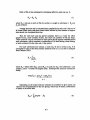
The catch rate estimate is the total number of fish caught divided by the number
of hours fished by all anglers interviewed during that time interval (eq. 2).
(2)
Sij = Ci/hij
where S.. = catch rates in number or weight of fish species per hour fished, C. =
total nubeir or weight of fish caught by anglers interviewed during the time interal
in i, and h.. = total number of hours fished (party size times hours fished at time of
each inter iew summed over all interviews in i, j).
A-1
Catch of fish is then estimated by multiplying effort by catch rate (eq. 3).
Hij = Eij"*Sij
(3)
where H. = harvest or catch of fish by number or weight in substratum i. Ei and
Sij are as above.
Average hours per trip is calculated from completed trips only and is the sum of
all hours fished (party size times hours fished) divided by total number of anglers
interviewed who completed their trips.
Thus for each date and day-period sampled, there is a value for effort
(angler-hours), catch (number of fish), and catch rate (number of fish per hour).
These statistical units are calculated for each species and all species combined within
each substratum, which comprise a combination of (a) boat fishing, shore fishing,
or both combined; (b) day type; and (c) day-period.
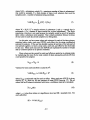
For each substratum and stratum, a mean (eq. 4) and a variance (eq. 5) is
calculated for each of the three primary statistical units in (1), (2), and (3) (adapted
from Cochran 1963):
X.•
i
(4)
X.
n
where X.. = either effort (Ei), catch (Hi.), or catch rate (S.. ) for substratum i and
sample j, and n = number of samples taken. Subscripts Por strata are omitted for
clarity.
VAR(X,) = 1(Xij) 2 - [(jXiU) 2/n]
(5)
n-1
Depending on the output desired, substrata are combined to give means and
variances for the parameters for the new groups, which may be strata, combinations
of strata, or the whole lake.
XST = =[(N/N)
"
(6)
Xi]
A-2
where N.N = substratum weight, Ni = maximum number of dates in substratum i
that could be sampled, N = total number of dates in all substrata that could be
sampled, and L = number of substrata being combined.
VAR(XST) =
L
[(W, 2 . Si2)/n.]
(7)
where W i = N/N, S.2 = sample variance in subtratum i, and ni = sample size in
substratum i (i.e., number of dates creeled for a given substratum). The finite
population correction is not used because the variance would be zero if all possible
dates within a substratum were sampled. This is clearly unrealistic because a census
of total catch in each day-period sampled is not being taken.
At this point, we have mean values and variances for each of the three primary
statistical units--catch, catch rate (CPUE), and effort--for the strata combination
selected for analysis. If the user has decided to group all sections of the lake and all
time periods together, we have a mean catch, catch rate, and effort for the whole lake
for the year. Mean catch and catch rate (CPUE) are expressed by number or weight
and by common species or all species combined.
Mean values per day-period for catch and effort are scaled up to estimate totals
by multiplying the mean by the total number of dates among day-periods (N) that
could possibly be sampled.
(8)
XToT = XST" N
Variance for total catch and effort is scaled by N2 :
VAR(XQr ) = VAR( XST) N2
(9)
where XTOT -=estimated total for catch or effort. Mean catch rate (CPUE) is given
directly by XST from eq. (6) and variance of mean CPUE from eq. (7). For all
values that have variances associated with them, a confidence interval is calculated.
(10)
X ± tt(SE)
where ta = t value from tables at a significance level and SE = standard error. For
catch and effort
SE=
IVAR (XTo)
A-3
and for CPUE
SE = (VAR ( XST)
Approximate
degrees
of freedom
[%(Ni2/)
. Si2] 2
1[((N_/ni2) . S.)/ni - ]
(11)
The number of trips is estimated by dividing total effort by the average hours
per trip. No variance is calculated.
References
Cochran, W.G. 1963. Sampling techniques, 2nd ed. John Wiley and Sons, New York.
A-4
I
I
I
i
^.^^I
^-.^-'I
I
I
I
I
I
I
I
I
I
I
I