Download fulltext - DiVA Portal

Computer Science, Degree Project, Advanced Course,
15 Credits
AUTONOMOUS WHEEL LOADER
SIMULATOR
Samuel Navas Medrano
Computer Engineering Programme, 180 Credits
Örebro, Sweden, Spring 2014
Examiner: Franziska Klügl
Örebro universitet
Institutionen för
naturvetenskap och teknik
701 82 Örebro
Örebro University
School of Science and Technology
SE-701 82 Örebro, Sweden
Abstract
The use of simulators when developing robotic systems provides the advantages of the
efficient development and testing of robotics applications, saving time and resources and
making easier publics demonstrations. This thesis project consists on the simulation of a
wheel loader at an industrial environment in the cycle of material handling.
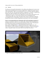
This report describes the development of a physics-based simulator using the Robot Operating
System (ROS) and Gazebo frameworks. The resulting simulator allows reproducing the 3D
map of the work site as well as the robotic wheel loader and simulating it in a realistic way.
The developed software also provides the mechanism to drive the wheel loader through the
reproduced terrain, to control the movement of the different articulated joints of the robot, to
receive information of the environment through different sensors and to provide of a waypoint
routes to the robot.
The simulator makes it possible to generate realistic data for mapping, localisation, and
obstacle detection -- using models of actual work sites. The simulator also will make it
possible to evaluate algorithms for task and path planning in a much more efficient way than
would be possible otherwise.
Summary
Autonomous Long-Term Load-Haul Dump Operations (ALLO) is a joint project by the
MR&O Lab, Volvo Construction Equipment, and NCC Roads. The goal of the ALLO project
is to find a solution to the demand for efficient material transport in many industrial
environments. The employment of autonomous mobile robots in the cycle of material
handling; including loading and unload the material is a solution which has a great potential
to offer improvements in terms of safety, cost, efficiency, reliability and availability.
This project consists on the analysis and porting of an old wheel loader simulator with the
Player/Stage framework from the ALLO Project to a modern robotic framework like Robot
Operating System (ROS) and Gazebo. The new simulator is able to reproduce a realistic
scenario as well as simulate a L120F Volvo wheel loader model.
The developed software also provides the mechanism to drive the wheel loader through the
reproduced terrain, to control the movement of the different articulated joints of the robot, to
receive information of the environment through different sensors and to provide of a waypoint
routes to the robot.
The simulator makes it possible to generate realistic data for mapping, localisation, and
obstacle detection, using models of actual work sites. The simulator also will make it possible
to evaluate algorithms for task and path planning in a much more efficient way than would be
possible otherwise.
The development of this simulator enables more rapid testing and development of the
algorithms developed within ALLO (compared to testing them on the hardware platform that
is available in Eskilstuna), And it makes it possible to create visual demonstrations for public
dissemination.
1 (26)
Preface
I would like to thank Martin Magnusson for giving me the opportunity to take part in this
project and for guide me through it.
2 (26)
Contents
1
INTRODUCTION ............................................................................................................ 4
1.1 OBJECTIVE .................................................................................................................. 4
1.2 BACKGROUND ............................................................................................................. 4
1.3 PROJECT ...................................................................................................................... 4
1.4 REQUIREMENTS........................................................................................................... 5
1.5 OUTLINE ...................................................................................................................... 5
2
METHODS AND TOOLS ............................................................................................... 6
2.1 METHODS .................................................................................................................... 6
2.2 TOOLS .......................................................................................................................... 6
2.2.1
Installation of the software tools ................................................................................................ 7
2.3 OTHER RESOURCES ..................................................................................................... 7
3
IMPLEMENTATION ...................................................................................................... 8
3.1 IMPLEMENTATION OF THE WHEEL LOADER AND SENSORS ......................................... 8
3.1.1
3.1.2
3.1.3
Model structure and measurements .......................................................................................... 8
Controllers .................................................................................................................................. 11
Sensors ....................................................................................................................................... 12
IMPLEMENTATION OF THE 3D MAP .......................................................................... 14
IMPLEMENTATION OF THE 3D MAP DEFORMATION ................................................. 15
IMPLEMENTATION OF THE PATH FOLLOWING.......................................................... 15
3.2
3.3
3.4
4
RESULTS ........................................................................................................................ 19
5
DISCUSSION ................................................................................................................. 20
5.1 ACHIEVEMENT OF THE COURSE OBJECTIVES ........................................................... 20
5.1.1
5.1.2
5.1.3
Knowledge and comprehension ............................................................................................... 20
Proficiency and ability .............................................................................................................. 20
Values and attitude ................................................................................................................... 21
COMPLIANCE WITH THE PROJECT REQUIREMENTS ................................................. 21
SPECIFIC RESULTS AND CONCLUSIONS...................................................................... 21
PROJECT DEVELOPMENT .......................................................................................... 21
5.2
5.3
5.4
6
REFERENCES ............................................................................................................... 22
APPENDICES
A: URDF hierarchy
B: Wheel Loader Simulator User Manual
3 (26)
1 Introduction
1.1 Objective
The purpose of emerging a visual simulator is twofold. First, it enables more rapid testing and
development of the algorithms (compared to testing them on the hardware platform), and
second, it makes it possible to create visual demonstrations for public dissemination.
The use of simulators when developing robotic systems provides the advantages of the
efficient development and testing of robotics applications, saving time and resources and
making easier publics demonstrations. This thesis project consists on the simulation of a
wheel loader at an industrial environment in the cycle of material handling.
The usage of a robotic simulator will offer advantages in terms of safety, costs, efficiency and
availability; as well as environmental advantages. All these advantages compared to testing
the algorithms on the real vehicle in its working.
1.2 Background
Mobile Robotics and Olfaction Lab (MR&O) is part of the Centre for Applied Autonomous
Sensor System at Örebro University. MR&O is focusing on research perception systems for
mobile robots and advance the theoretical and practical foundations that allow mobile robots
to operate in an unconstrained, dynamic environment.
Autonomous Long-Term Load-Haul Dump Operations (ALLO)[1] is a joint project by the
MR&O Lab, Volvo Construction Equipment, and NCC Roads. The goal of the ALLO project
is to find a solution to the demand for efficient material transport in many industrial
environments. The employment of autonomous mobile robots in the cycle of material
handling; including loading and unload the material is a solution which has a great potential
to offer improvements in terms of safety, cost, efficiency, reliability and availability.
A previous approach on this project was the development of a wheel loader simulator (using
Gazebo[2]) with the Player/Stage framework[3][4]. The simulator was used both for algorithm
testing and for preparing demos without running the real wheel loader. But the code of the
ALLO project was migrated to the ROS framework rather than player stage, with the Hydro
version of ROS a simulator can be develop using the version 1.9 of Gazebo rather than the 0.8
version that used the previous ALLO’s simulator.
1.3 Project
The first task of the project has been the analysis the previous simulator written in
Player/Stage and the research of the different ways to improve it, including what robotic
framework could be better to our project[5][6]. The next task have been to port what is there
from Player/Stage to the chosen framework, resulting in a simulator that can be used to
visualize the wheel loader in its environment and to collect simulated laser and position data.
4 (26)
1.4 Requirements
The requirements have divided in three steps, the first one had high priority and the rest were
optional. In each one the simulator had the following capabilities:

Step I (high priority):
o Gazebo simulator
o Ability to use 3D maps of work site (Kjula)
o Ability to drive articulated wheel-loader model interactively
o Simulated sensors: laser scanners, odometry, GPS, IMU

Step II (optional):
o Ability to replace part of the 3D map: for when the piles change after a bucket
fill
o Ability to follow a given path (given as a list of waypoints), with a given speed
(+- some variance)

Step III (optional):
o "Asphalt plant model": that is, maintaining a representation of the gravel level
in bins, and emptying rates for a given recipe, +- some variance in levels and
emptying rates
o An interface for getting and setting parameters for the simulation from the
outside, developed in dialogue with the ALLO project.
All the goals have been fulfilled, with the exception of given a speed in the path following
goal and the implementation of the asphalt plant model.
1.5 Outline
The structure of the remainder of the document is as follows. Section 2 describes the tools and
basic setup that has been used. Section 3 contains much of the core of the work, as it details
the implementation of the simulator's components. Section 4 details the results of the project
and Section 5 discuss the reached competences during the course of the project.
5 (26)
2 Methods and tools
2.1 Methods
During the project have been used an incremental development model with some iterative
elements. An initial set of requirements have been established at the beginning of the project
and it has been redefined during the course of the project during weekly meetings with the
client, the researchers working in the ALLO project.
2.2 Tools
ROS (Robotic Operating System)[7][8] is the main development framework used in this
project. It is an Open Source framework which has tools for the building of robotics
applications and is maintained by the community in a very collaborative environment.
ROS provides libraries and tools to help software developers create robot applications. In
addition also Gazebo Simulator was used complementing ROS, it offers the ability to
accurately and efficiently simulate robots in complex indoor and outdoor environments and
has a wide variety of physics engine including ODE, Bullet, Simbody and DART. Using
OGRE, Gazebo also provides a realistic high-quality graphics including high-quality lighting,
shadows, and textures. Gazebo also has a convenient programmatic and graphical interface.
The documentation of ROS, the wiki and tutorials, and the Q&A site have been a great
support during the course of the project.
The ROS community has over 1,500 participants on the ros-users mailing list, more than
3,300 users on the collaborative documentation wiki, and some 5,700 users on the
community-drivenROS Answers Q&A website. The wiki has more than 22,000 wiki pages
and over 30 wiki page edits per day. The Q&A website has 13,000 questions asked to date,
with a 70% percent answer rate.
(http://www.ros.org/, 2014)
Reusing these libraries for the development of the simulator is possible because of the
generous software licenses used by ROS and Gazebo. The core of ROS licensed under the
standard three-clause BSD which is a very permissive licence that allows for reuse in
commercial and closed products; the other parts of ROS like community packages usually
uses licences such Apache 2.0 licence, GPL licence, MIT licence.
Gazebo requires a graphic card with OpenGL 3D acceleration to perform various rendering
and image simulation tasks correctly. But it can still working without it at the expense of not
having camera simulations and a working Gazebo UI. But even with these disadvantages it is
still useful for testing algorithms.
A laptop with a dedicated graphic card has been used for develop the project. A Lenovo
IdeaPad Z580 with a Intel(R) Core(TM) i7-3612QM CPU @ 2.10GHz CPU working a Nvidia
Optimus configuration with the following GPUs: NVIDIA GeForce GT 630M & Intel(R) HD
Graphics 4000.
6 (26)
Also additional software has been used in this project:
 Ubuntu 13.04 (Raring)
o Bumblebee (v Ubuntu 12.10)
 Windows 7
o Adobe Photoshop CS6 Extended
o NVIDIA Texture Tools for Adobe Photoshop
o Blender 2.63a
2.2.1
Installation of the software tools
During the project it has been used ROS: Hydro Medusa, this version of ROS only supports
Ubuntu 12.04 (Precise), Ubuntu 12.10 (Quantal), and Ubuntu 13.04 (Raring). It has been
installed the latest version of the supported Ubuntu releases: Ubuntu 13.04. The full desktop
package of ROS hydro also includes the stand-alone version of Gazebo 1.9 and the libraries
for the ROS/Gazebo communication. There is also a newer version of Gazebo (2.0) but the
newer version is not compatible with ROS Hydro Medusa
To work properly with a 3D environment simulator like Gazebo we should work with a
dedicated graphic card. The computer we have used to the development of the project has the
technology NVIDIA Optimus [9]. This is not supported out of the box by Ubuntu 13.04. Some
hybrid graphics laptops still allow you to choose using only the nVidia card in BIOS, but most
modern Optimus laptops don't have this option.
It is possible to solve this issue with the installation of the Bumblebee Project [10]. It is a set of
tools developed by people aiming to provide Optimus support under Linux. Bumblebee
doesn’t have a release for Ubuntu 13.04 in their official repository; the only way to use it is
installing the version of Bumblebee to Ubuntu 12.10. Due to this lack, it is necessary to
modify the manual configuration of the Bumblebee files and indicate to it to use specifically
the PCI Bus ID of our NVIDIA GPU.
2.3 Other resources
All the needed data 3D maps of the terrain, the Volvo’s L120F wheel loader 3D model, the
code of the old simulator, external algorithms (path planning, task scheduling, and gravel
simulation), path data and all required information related to the project have been supplied
by the ALLO Project.
7 (26)
3 Implementation
3.1
3.1.1
Implementation of the wheel loader and sensors
Model structure and measurements
The first step to implement a realistic simulation of a Wheel Loader in gazebo is to build the
3D model of the wheel loader machine. The 3D model of the previous implementation of the
wheel loader from the ALLO Project is not compatible with our version of Gazebo. However
it has been able to reuse some information of the previous model, like the hierarchy of the
joints of each part of the body of the model and estimate the dimension of these parts.
Two different approaches were considered for the building of the new L120F model: try to
use all the possible information about the old model and follow it structure or build a
completely new one model. In order to reuse as much software and data from the Player/Stage
simulator, It has been made the design choice of adapting the previous model to the new
URDF format. The creation of a completely new model would be better in terms of accuracy
but it has been considered it not a priority, leaving this option to a future development of the
project. Respect to the dimensions of the resulting model it has been approached to the
dimensions of the Volvo’s L120F technical specifications [11] and the dimensions of the model
of the previous simulator.
Like in the old code, it have been used the basic geometric shapes which Gazebo uses to build
the model. The wheels are represented by cylinders and the other structures like the rear
frame, the suspension, the articulated arm, etc. are represented by cuboids (boxes). For the
pieces that before were represented by meshes, the front frame and the bucket, the first
approach was represent it as boxes of an approximated size, but later them I replaced it
modelling a new COLLADA meshes using Blender. (See Figures 3.2.2 and 3.2.5).
The format which gazebo uses to the description of robot models is Simulator Description
Format (SDF) but It has been parsed all the information of the previous project model to the
Unified Robot Description Format (URDF) and it has been used the XACRO tool to clean up
our URDF files. It has been chosen this format instead of SDF because is the most extended
and standardized XML format for the description of robots.
However, in the process of the reconstruction and parsing of the previous model into de
URDF format we have discovered some issues. The first is that some features of URDF have
not been updated to deal with the evolving needs of robotics. URDF can only specify the
kinematic and dynamic properties of a single robot in isolation, neither can specify the pose of
the robot itself within a world. This is not a big deal because Gazebo is going to solve these
points; however there is a problem which gazebo can’t deal with it, the hierarchical data
structure in URDF that does not allow for loops (parallel joints) that the previous model of the
wheel loader has in the mechanical arm structure.
The wheel loader XML model of the player/stage simulator uses joint loops for the
representation of the mechanical arm of the Volvo L120F vehicle. A way to solve this problem
is the use of SDF models and assigning <pose> in joint loops to create parallel mechanisms,
however it have been opted for simplifying the model removing the joint loops and let the
task of developing a more realistic model to a future.
8 (26)
Another difference with the specification of the old L120F model and the new one is the fact
that the older specify the position of all the pieces of the model in their body’s tags. The
equivalent of that in our model are the link’s tags, but we cannot define the position of each
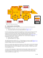
piece there because two reasons, the main reason is for modelling the articulated joints, "we
need to compute the difference between the position of the articulated joint and the geometric
centre of the link". The other reason is related to the fixed joints; we need to define the
location in the joints tags because if not the centre of mass of each piece will be in the origin
instead on the centre of each piece. A graphic representing the resulting URDF hierarchy can
be seen in Appendix A.
The units of measure of the old model are also different to the URDF standard, for example
the angles in the old model are represented in degrees and we are representing it in radians to
follow the URDF standard. Another measure is the mass; Gazebo 1.9 doesn’t manage well the
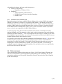
physics of body with huge masses provoking the explosion of the model. Finally it has been
adopted masses of approximately of 1 kilogram in each piece of the wheel loader. The final
dimensions of each body of the L120F model can be seen in the Figure 3.2.1.
In addition, the previous meshes of the L120F model were compiled in OGRE but in a
previous version that Gazebo 1.9 doesn’t recognise, it have been converted the compiled
meshes back to their original OGRE XML files using the OgreXMLConverter tool [12] and it
has been tried to convert it to another format which Gazebo load. But, due to the low
complexity of the meshes we have decided that will be easier and quicker to remake using
Blender [13] the front frame and bucket meshes in the COLLADA XML format than convert
the previous one to it.
Body
Rear frame
Counter weight
Front frame
Rear suspension
Right rear wheel
Right front wheel
Left rear wheel
Left front wheel
Articulated arm
Bucket
Type
Box
Box
Box
Box
Cylinder
Cylinder
Cylinder
Cylinder
Box
Box
Dimensions
w=2 h=2 d=3
w=3 h=1 d=1
w=2 h=2 d=2
w=2 h=0.3 d=0.3
r=0.6 h=1
r=0.6 h=1
r=0.6 h=1
r=0.6 h=1
w=1 h=4 d=0.2
w=2 h=1 d=1
Figure 3.2.1: L120F model measurements, in meters.
Another issue on the parsing of the model is that the previous version has not specified
information about the inertia of the pieces of the model, but in our actual version of Gazebo
and ROS is necessary to specify the inertia in the model. The inertia tensor encodes the mass
distribution of a body, so it does depend on the mass, but also on where it is located and is
represented in URDF with the diagonal and upper elements of a symmetric matrix. One of the
possible solutions is to use an identity inertia matrix as default in the model. Another solution
is the using of inertias of 1e-3 or smaller like elements in the inertia matrix because 1 is often
much too high, making the model hard to drive, with an unnatural behaviour.. The usage of a
default inertia matrix is enough for the purpose of the project, but a calculated inertia mass for
each piece will be a more complete and realistic solution, having as result a more precise and
realistic simulation. The inertia matrix has been calculated according to a list of moment of
9 (26)
inertia tensors using the uos_tools package from the University of Osnabrück, knowledge
based systems group [14]:
1
12
𝑚(3𝑟 2 + ℎ2 )
1
12
2
0
0
𝑚(3𝑟 2 + ℎ2 )
2
2
0
1
12
𝑚𝑟 2
*
]
0
𝑚(𝑤 2 + 𝑑 2 )
0
0
1
0
𝑚(ℎ +𝑑 )
0
[
12
0
[
𝐼𝐶𝑈𝐵𝑂𝐼𝐷 =
1
0
𝐼𝐶𝑌𝐿𝐼𝑁𝐷𝐸𝑅 =
0
0
1
12
𝑚(𝑤 2 + ℎ2 )
**
]
* Solid cylinder of radius r, height h and mass m.
** Solid cuboid of width w, height h, depth d, and mass m.
(www.wikipedia.org, 2014)
The ICYLINDER matrix has been applied to the wheels, and the ICUBOID matrix to the rest of the
pieces of the model. It has been simplified the inertia of the pieces represented by meshes like
if it were cuboid, using the dimensions of their bounding boxes. (See Figure 3.2.2).
Another detail about the inertia of each body of the model and the centre of mass of them is
that URDF have to specify the location of each model in the joints tags, instead of in the link
tags like the previous model, if not the inertia matrix will be ignored and the centre of mass of
each body in the model with be the origin of the model.
It can be also modified the damping of the joints. By default in URDF the joints have 0
dumping on the controlled position joints (the steering joint, the mechanical arm and the
bucket) when we try to move some joint and it arrive to the desired position, the joint starts to
bounce and finally converge to the position. It has been reduced on the mentioned joints the
dumping force to -50 Newton meter seconds per radian. A -50 value shows a realistic
dumping, but you can reduce the dumping until -300, if it is reduced more the dumping the
model it will destroy.
Related to the friction, is possible to modify the friction related to each material, modifying
the two friction coefficients of each material, which specify the friction in the principle
contact directions (as defined by the ODE physics engine used by Gazebo). These tags
represent the friction coefficients μ for the principle contact directions along the contact
surface as defined by the ODE physics engine of Gazebo. Is also possible modify the friction
related of each joint in the <friction> tags of the joints. It has been defined the coefficient of
the wheels material, the kinetic coefficient like 0.68 and the static like 0.9. This is the
coefficient of dry rubber on asphalt [15].And It has been defined the friction of the mobile
joints with 50. But changing these values doesn’t show any significant change on the
behaviour of the vehicle.
The only physical engine with works with a full functionality in Gazebo is Open Dynamics
Engine (ODE) [16], when I tried to use the Bullet engine [17] instead of ODE, Gazebo would
not load at all because the Bullet integration in Gazebo 1.9 is still experimental.
10 (26)
3.1.2
Controllers
Once the 3D model of the wheel loader was constructed, the next step was the implementation
of a control system to grant movement to the model. There are a lot of alternatives to perform
this; if we were a bigger project the ideal way to control the model will be to make our own
gazebo model plugin and create our own gazebo custom messages model.
But another simplest and efficient way to implement it is to use the gazebo_ros_control
plugin, it have all the resources we need to implement a good way to control the movement of
the robot and it is a standard plugin of Gazebo/ROS and uses the standard messages
(std_msgs) of Gazebo, that means that the control mechanism will be easier to understand for
a person who incorporates to the project later and the control mechanism will be easier to
enlarge also in a future if we want to enhance the movement mechanism.
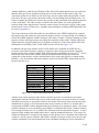
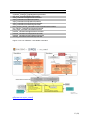
Ros_control libraries works like a controller interface between the ROS controller manager
mechanism and the hardware interface whether it is real hardware or simulated hardware by
Gazebo, as represents the Figure 3.2.3. We were able to use different interfaces to make
possible the communication between the control manager and the robot’s hardware. This
communication works using “topics”, different modules of our software publish information
about the robot in these topics, and some modules subscribe the information in these topics. It
has been used the JointStateInterface to allow ROS read information about the robot joints in
Gazebo. The EffortJointInterface allows ROS to send to Gazebo how the robot has to behave
(wheels, mechanical arm, etc.). It would be better to use a VelocityJointInterface to manage
the rotation velocity of the wheel joints of the robot, but that interface is not fully
implemented in Gazebo 1.9. The problem using a force control instead a velocity control is
that is hard to maintain a reasonable speed on bumpy ground, like the ground of the
Eskilstuna terrain in the simulation.
The EffortJointInterface offer to us different kind of controllers to change the parameters of
the joints of the robot (It can be seen a list of all the available controllers of Gazebo at the
Figure 3.2.4). I have used the JointPossitionController to change the position of the articulated
joints, like the direction joint between the rear frame and the front frame and also for the
articulated joints of the mechanical arm and the bucket of the L120F wheel loader.
About the control of the rear wheels, it has been tested the
diff_drive_controller/DiffDriveController, velocity_controllers/JointVelocityController,
effort_controllers/JointVelocityController, and the effort_controllers/JointEffortController.
The first two controllers wasn’t able to load by Gazebo, the third loads but makes the model
crash (the joint hierarchy is destroyed and Gazebo visualizes al the joints together, without
any sense), and I only could load the JointEffortController, this controllers makes possible to
spin the wheels and move de vehicle, but we cannot control the velocity of it, for example,
with the same effort the velocity will be different if the vehicle is climbing a hill o driving in a
flat ground. All the controllers can be seen in the Figure 3.2.4.
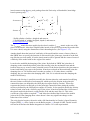
With the action of the controllers of these interfaces the L120F robot will modify the
respective properties of each joint when it receive a standard message in each controller, It has
been written a UNIX Bash Script to automate the sending of messages and to have an
intuitive way to drive and control the articulated wheel-loader model interactively by
keyboard. It has been chosen the use of UNIX shell scripting instead C++ due to the facility
of the implementation and the absence of the necessity of compile the code after each small
11 (26)
change and the necessity of being multiplatform.
3.1.3
Sensors
The final step in the model implementation is the addition and configuration of sensors to the
model. It has been added a laser scan sensor configured like a Hokuyo laser to the top to the
wheel loader machine. With it a semi-translucent laser ray is visualized within the scanning
zone of the GPU laser. This can be an informative visualization, or a nuisance. In addition, the
Hyokuo laser plugin will publish all the data obtained from the sensor to the
“/l120f/laser/scan” topic. It has been also implemented a camera sensor which publish on the
“/l120f/camera1/image_raw” topic and an Odometry sensor which publish on the
“/l120f/odometry/data” topic. After a meeting with the client the configuration of the laser
was changed to be like a SickLMS200 scanner, the same sensor that uses the old simulator
from the ALLO Project. And more importantly, the same that we use on the real machine.
However, it has been decided not to implement the GPU, IMU and Odometry sensors, these
sensors aren’t included in the gazebo_ros libraries and we have to depend of community
packages to implement it. Due to we are working with a simulation, this information can be
obtained directly from Gazebo instead from the simulation of these sensors. Nevertheless I
have looked for the packages what should implement leaving sensors: the
hector_gazebo_plugings package [18] implements different sensors plugins, like a 6dw
differential drive, an IMU sensor, an Earth magnetic field sensor, a GPS sensor and a sonar
sensor. Another option for an IMU sensor plugin is the microstrain_3dmgx2_imu plugin [19]
which is compatible with the microstrain 3DM-GX2 and 3DM-GX3 protocol.
Figure 3.2.2: Bounding box of the bucket’s mesh.
12 (26)
Available controllers
controller_manager_tests/EffortTestController
controller_manager_tests/MyDummyController
diff_drive_controller/DiffDriveController
effort_controllers/GripperActionController
effort_controllers/JointEffortController
effort_controllers/JointPositionController
effort_controllers/JointTrajectoryController
effort_controllers/JointVelocityController
force_torque_sensor_controller/ForceTorqueSensorController
imu_sensor_controller/ImuSensorController
joint_state_controller/JointStateController
position_controllers/GripperActionController
position_controllers/JointPositionController
position_controllers/JointTrajectoryController
velocity_controllers/JointVelocityController
Figure 3.2.3: List of Gazebo 1.9 available controllers
Figure 3.2.4: Data flow of ros_control and Gazebo
(http://wiki.ros.org/ros_control)
13 (26)
IMU
GPS
Laser
Position
Position
Controller
Controller
CAM
Counter
wheight
Arm
Rrear Frame
Buck
Front Frame
Front
Wheel
Rear
Wheel
Legend:
Links
Controllers
Effort
Controller
Without
Controller
Articulated
Joints
Figure 3.2.5: L120F model structure
3.2 Implementation of the 3D Map
For the implementation of the 3D Map it has been received from the ALLO project the
following files:
 Two 32bits RGB PNG 1000x1000 pixel heightmaps (Figure 3.2.1 a, b).
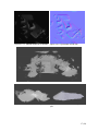
 A PLY mesh with 411958 vertices and 661609 faces. (Figure 3.2.2).
It has been started trying to implement the heightmap system because the triangle mesh that
was received from the ALLO Project is too huge to have a good performance with it; a
heightmap is much softer and more efficient. A heightmap can also represent the surface
elevation data of the ground where the asphalt plant is in Eskilstuna-Kjula (Figure 3.2.1 a, b)
for its representation on the Gazebo environment. To do it first it has been adapted the
heightmap to the Gazebo 1.9 requisites:
 A 8bits square greyscale image
 Each side must be (2^n)+1 pixels
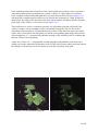
The PNG file has been resized to a 513 x 513 pixels image as we can see in the Figure 3.2.1 c
using Photoshop. It has been also generated a normal map as we can see in the Figure 3.2.1 d
using the NVIDIA Texture Tools for Adobe Photoshop [20].
However, the wheel loader model doesn’t behaviour correctly when it is tried to drive thought
the generated terrain, and in addition, the latest versions of Gazebo, including the 1.9 version,
has several bugs in the uses of the heightmaps, related to the physics, collisions and textures
of the heightmap’s terrain.
As result we had contemplate to implement the terrain map with a triangle mesh. It has been
received from the ALLO Project another 3D mesh in COLLADA format which is just a
simplified fragment of the original previously mentioned Kjula 3D map with only 24912
vertices and 49999 faces (Figure 3.3.2).
14 (26)
3.3 Implementation of the 3D Map Deformation
The implementation of the 3D Map deformation has been motivated due to the necessity of
visualize the effect of the gravel simulation algorithm form the ALLO Project in the gravel
piles when the wheel loader takes material from them. Gazebo doesn’t have a lot of variety of
options to implement the change or update of a mesh in simulation time. One possible option
for the implementation of the map deformation is having the variable parts of the terrain like a
different mesh. In this way Gazebo has a helper script called spawn_model is provided for
calling the model spawning services offered by gazebo_ros.
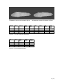
It has been received from the ALLO project three COLLADA triangle meshes of the different
levels of a grave pile (Figure 3.3.1 b, c, d). These meshes have been computed using the
ALLO Project gravel simulation algorithms. And using the gazebo spawn service we can
delete a model of a pile and replace it with the same model modified in simulation time.
However, the Gazebo’s spawn scripts have some issues and we can’t spawn two times a
model with the same name, so when was implementing the changing of a mesh in simulation
time on the existing bash script of keyboard control I had to count the times I was spewing the
model and change its name to pile-n where n is {0, 1, 2 … n}.
3.4 Implementation of the Path Following
Related to the ability to follow a given path, first It has been looked for some Gazebo and
ROS official libraries to help to perform it but it has been found only libraries of path
planning, these are the ROS 2D Navigation stack [21] and the Motion Planners stack [22] ; they
take information from odometry and sensors streams and output velocity commands to send
to a mobile base.
We want a simpler solution, our wheel loader will move in the same map doing a repetitive
movement, from the gravel piles to the asphalt plant’s containers. In this project it is not going
to explore a new map. We rather want to use it to try out our algorithms for navigation,
motion planning, etc. So we only need to receive information about the location of the robot
in our known map and depending of this location send to it new data about it velocity and
orientation.
It has been used the P3D (3D Position Interface for Ground Truth) controller plugin, this
plugin simulate an odometry sensor and sends this information about the pose and orientation
of the vehicle to ROS through a ROS topic using nav_msgs/Odometry ROS messages. I have
configured this plugin to use the position of the rear frame as reference to take the odometry
information and sent via the “base_pose_ground_truth” topic.
The next step was to develop a ROS subscriber C++ program to correctly receive and
interpret the odometry information of the vehicle from the topic; I have taken as a reference
the code of the “Writing a Simple Publisher and Subscriber” tutorial from the ROS wiki. Once
we received a message from the topic we can be able to extract the X and Y coordinates from
the pose of the vehicle and the quaternion of its orientation and then converts it to pitch, from
the roll/pitch/yaw vehicle orientation system, using the following equation:
𝑃𝐼𝑇𝐶𝐻𝐴𝑁𝐺𝐿𝐸 = 𝑎𝑡𝑎𝑛2(2 (𝑦𝑥 + 𝑤𝑧), 𝑤𝑤 + 𝑥𝑥 − 𝑦𝑦 − 𝑧𝑧
15 (26)
Now, with the position and orientation of the vehicle I had to develop the way to represent a
path and send the property information to vehicle to follow it. I have taken as a reference
some examples of back-and-forths path that I received from the ALLO Project Figure 3.4.1.
and then I have implemented a simpler way to describe the waypoints of a path, using only
the position, the angle of the direction joint of the wheel loader (in radians) and the expected
pitch angle of the vehicle, as we can see in the Figure 3.4.2.
Then each time we receive a odometry message, the subscriber program will check if the
vehicle is in the x and y coordinates of the corresponded waypoint, and if it fits (with a
determined offset margin) it will publish the new position of the direction joint to the wheel
loader, then it will start to turn and when it reach the corresponding pitch angle (also with an
offset margin) the C++ program will publish a message to the direction joint of 0 radians and
then the vehicle will stop turning.
At the end we have a C++ program that is ROS subscriber and publisher at the same time
which receives the odomertry information of the L120F wheel loader vehicle and sent to them
the changes of the direction of it movement to reach the waypoints of the path.
Figure 3.2.1 a: grid overlayed heightmap.
Figure 3.2.1 b: heightmap.
16 (26)
Figure 3.2.1 c: adapted heightmap to Gazebo.
Figure 3.2.1 d: generated normal map.
Figure 3.2.2: Kjula PLY mesh.
Figure 3.3.1 a: Kjula simplified triangle mesh.
Figure 3.3.1 b: scan data from a real gravel
pile.
17 (26)
Figure 3.3.1 c: the same pile after having
simulated the removal of 5 buckets of gravel.
distance
front x
front y
front
angle
Figure 3.3.1 d: the same pile after having
simulated the removal of 49 buckets of gravel.
waist
angle
rear x
rear y
rear
angle
waist
angle
speed
0
0
0
0
0.196
-3.196
0.312
-0.196
-0.107
0.105
0.105
0
0.012
0.207
-3.064
0.291
-0.195
-0.118
...
...
...
...
...
...
...
...
...
Figure 3.4.1: ALLO Project path description.
rear x
rear y
front
angle
pitch
angle
wheels
effort
-20.0
-20.0
-20.0
6.0
0.0
-0.25
0.0
-0.80
-2.0
-2.0
…
…
…
…
…
Figure 3.4.2: Actual path description.
18 (26)
4 Results
The result of the project has been evaluated by the researchers of the ALLO Project. They are
generally happy with the state of the simulator.
The final point of the requirements (interface for communicating with the simulation) is
actually quite important, and it's good to see that it is in place (using the ROS topics
listed in the user manual). Since Rviz can show the poses of all the links of the vehicle
and the simulated laser data, that also means that the output of the simulator looks
(essentially) the same to our software as the data from the real robot.
The main issue with the current simulator is the lack of velocity control. Given that this
controller is not fully functional in Gazebo 1.9, it is understandable that it wasn't
implemented, but that is something we will need to work around for future development
of the simulator.
(Magnusson, Martin; result notes from the ALLO Project)
The resulting code of the simulator is also well documented and easy to use in a future
development.
19 (26)
5 Discussion
5.1
5.1.1
Achievement of the course objectives
Knowledge and comprehension
During this project it has been acquired deep theoretical knowledge in rigid body simulation
that is being performed by Gazebo. And it has been acquired following competences:
 Work with an officially unsupported GPU in Ubuntu 13.04 using Bumblebee.
 Install and Configure a ROS and Gazebo Environment.
 Navigate the ROS Filesystem and create the ROS packages following the catkin
standard.
 Understand ROS Nodes, Topics, Services and Parameters.
 Build and modify a Gazebo world.
 Build a physical realistic robot using URDF and XACRO.
 Use a URDF model in Gazebo.
 Use a heightmap in Gazebo.
 Make SDF models.
 Import and attach meshes to the URDF and SDF models.
 Add different sensors to a robot.
 Use Gazebo plugins in ROS.
 Work with the gazebo_ros_control plugin for the ROS communication with Gazebo.
 Publish into a ROS topic to modify the state of a robot’s joint in Gazebo.
 Subscribe into a ROS topic to show information about the robot in Gazebo in Rviz.
5.1.2
Proficiency and ability
During this project it has been acquired the following abilities:
 Draft and define the technological problem of the realistic simulation of robotic
hardware and rigid bodies.
 Search for scientific information to solve these problems in scientific databases such
as IEEE Explore[23] and Google Scholar[24].
 Plan and implement a technological project in a professional environment, using an
incremental development model with some iterative elements. Defining an initial set
of requirements and redefining them during the course of the project.
 Process and analyse scientific results as it can be seen in the results section.
 Have the ability to present the project orally and writing.
 Have control of planning, monitoring and implementation between the whole project
periods as it can be seen in the schedule of the specification of the project.
 Write emails and plan weekly meetings with the staff from the ALLO Project.
20 (26)
5.1.3
Values and attitude
During the project it has been acquired the following values:
 Have the ability to stay informed about current knowledge/research development and
working methods used in the field as it can be seen during the course of the project, in
the report, in the results and in the references of the report.
 Have a professional approach in their relationships with the ALLO Project. It has been
doing regular meetings during the project, maintained active communication by email
with members of the ALLO Project and receiving feedback from them about the result
of the project and the changes in the requisites.
 Have a professional approach to the end product of the project. The resulting software
of the project has been developed making particular emphasis on the reliability,
usability, extensibility, documentation and the reutilization of the software.
5.2 Compliance with the project requirements
The high priority Step I of the project consisting on the installing and configuration of the
Gazebo/ROS environment, the recreation of the Kjula map into the simulator and the ability
of drive the wheel loader through the terrain have been completed in their majority.
Also the optional Step II consisting on the ability to replace part of the 3D map to another and
the ability of the vehicle to follow a path given a list of waypoint have been also completed.
Related to the Step III it has been done an interface for the ALLO Project, using the ROS
topic structures. Only it has not been completed the asphalt plant model due to it has been
dedicated more resources to solve and improve the others aspects of the simulator.
Even the uncompleted aspects, the project is a suitable solution to the problem presented from
the ALLO Project of the porting and development of their previous simulator.
5.3 Specific results and conclusions
It is possible to simulate the behaviour of a wheel loader vehicle in a realistic environment
using ROS and Gazebo in spite of their limitations. And will be interesting to continue the
development of the simulation at the same time as Gazebo and ROS grow.
5.4 Project development
The simulator has been developed following the standards in the using of the ROS and
Gazebo frameworks, which allows an easy expansion of it and its functionalities. Expand and
enhance the project should be able in the future at the same time that ROS and Gazebo grows.
Examples of tasks, which should be developed in the future, are the following:
 Complete the Step III of the project.
 Enhance the L120F Prototype with a more realistic physics and visuals.
 Enhance the driving mechanism of the vehicle.
o Have a better control of the velocity of the vehicle.
 Extend the path following mechanism.
o Read the path format from the ALLO Project.
 Change the usage of the standards libraries, plugins and messages for its own, more
adapted to the needs of the project.
21 (26)
6 References
[1] Magnusson, Martin; Cirillo, Marcello; Kucner, Tomasz, Automomous Long-Term LoadHaul-Dump Operations Project. Accessed 16 of June, 2014.
URL: http://aass.oru.se/Research/mro/allo/
[2] Koenig, Nathan & Howard, Andrew, Gazebo-3D Multiple Robot Simulator with
Dynamics. Accessed 16 of June, 2014.
URL: https://www.gazebosim.org
[3] Hedges, Reed; Støy, Kasper; Bers, Josh; Douglas, Jason K; Jinsuck, Kim; Martignoni III,
Andy; Melchior, Nik; Østergaard, Esben; Sweeney, John; Batalin, Maxim; Burns,
Brendan; Douglas, Jason K; Dahl, Torbjørn; Fredslund, Jakob; Jung, Boyoon; Dandavate,
Gautam; University of Melbourne RoboCup Team , Player Project.
Accessed 16 of June, 2014.
URL: http://playerstage.sourceforge.net/
[4] Gerkey, Brian; Vaughan, Richard; Howard, Andrew, “The player/stage project: Tools for
multi-robot and distributed sensor systems”. Proceedings of the 11th international
conference on advanced robotics, 2003, (ICAR 2003), pp 317-323, Coimbra, Portugal.
Accessed 16 of June, 2014.
URL: http://robotics.usc.edu/~gerkey/research/final_papers/icar03-player.pdf
[5] Koenig, Nathan & Howard Andrew, “Design and Use Paradigms for Gazebo, an OpenSource Multi-Robot Simulator”. Intelligent Robots and Systems, 2004, (IROS 2004).
Proceedings. 2004 IEEE/RSJ International Conference on; 2004. Robotics Research
Labs, University of Southern California, Los Angeles, CA 90089-0721, USA. Accessed
16 of June, 2014.
URL: http://robotics.usc.edu/~gerkey/research/final_papers/icar03-player.pdf
[6] Cousins, Steve; Gerkey, Brian; Conley, Ken; Staff from Willow Garage, “Sharing
Software with ROS”. IEEE Robotics & Automation Magazine, June, 2010, pp 12-14.
Willow Garage, Menlo Park, CA, USA. Accessed 16 of June, 2014.
URL: http://ieeexplore.ieee.org/stamp/stamp.jsp?arnumber=05480439
[7] Willow Garage, ROS: Robot Operating System. 2014. Menlo Park, CA: Willow Garage.
Accessed 16 of June, 2014.
URL: https://www.ros.org
[8] Quigley, Morgan*; Gerkey, Brian**; Conley, Ken**; Faust, Josh**; Foote, Tully**; Leibs,
Jeremy***; Berger, Eric**; Wheeler, Rob**; Ng, Adrew*,“ROS: an open-source Robot
Operating System”. Proc. Open-Source Software workshop of the International
Conference on Robotics and Automation (ICRA), 2009.
*
Computer Science Department, Stanford University, Stanford, CA.
**
Willow Garage, Menlo Park, CA.
***
Computer Science Department, University of Southern California.
Accessed 16 of June, 2014.
URL: http://ai.stanford.edu/~mquigley/papers/icra2009-ros.pdf
22 (26)
[9] NVIDIA Corporation, Whitepaper NVIDIA’s Next Generation Notebook Technology:
OptimusTM. Accessed 16 of June, 2014.
URL: http://www.nvidia.com/object/LO_optimus_whitepapers.html
[10] The Bumblebee Project. Accessed 16 of June, 2014.
URL: http://bumblebee-project.org/
[11] Volvo Corporation, Volvo Wheel Loaders L110F, L120F. Accessed 16 of June, 2014.
URL: http://www.volvoce.com/SiteCollectionDocuments/VCE/Documents%20Global/w
heel%20loaders/ProductBrochure_L110F_L120F_EN_21C1002738_2009-08.pdf
[12] OGRE – Open Source 3D Graphics Engine. Accessed 16 of June, 2014.
URL: http://www.ogre3d.org/
[13] Günther, Martin; Sprickerhof, Jochen, UOT_tools. Accessed 16 of June, 2014.
URL: http://wiki.ros.org/uos_tools
[14] Blender Foundation, The Blender project - Free and Open 3D Creation Software.
Accessed 16 of June, 2014.
URL: http://www.blender.org/
[15] Wikibooks. Physics Study Guide/Frictional coefficients. Accessed 16 of June, 2014.
URL: http://en.wikibooks.org/wiki/Physics_Study_Guide/Frictional_coefficients
[16] Smith, Russell. Open Dynamics Engine. Accessed 16 of June, 2014.
URL: http://www.ode.org/
[17] Coumans, Erwin. Bullet physics engine. Accessed 16 of June, 2014.
URL: http://bulletphysics.org/
[18] Meyer, Johannes; Kohlbrecher, Stefan, Hector_gazebo_plugins.
Accessed 16 of June, 2014.
URL: http://wiki.ros.org/hector_gazebo_plugins
[19] Leibs, Jeremy; Gassend, Blaise, microstrain_3dmgx2_imu. Accessed 16 of June, 2014.
URL: http://wiki.ros.org/microstrain_3dmgx2_imu
[20] NVIDIA Corporation, NVIDIA Texture Tools for Adobe Photoshop.
Accessed 16 of June, 2014.
URL: https://developer.nvidia.com/nvidia-texture-tools-adobe-photoshop
[21] Marder-Eppstein, Eitan, 2D navigation stack. Accessed 16 of June, 2014.
URL: http://wiki.ros.org/navigation
[22] Chitta, Sachin, Motion_planners stack. Accessed 16 of June, 2014.
URL: http://wiki.ros.org/motion_planners
[23] Institute of Electrical and Electronics Engineers. IEEE Xplore Digital Library.
Accessed 16 of June, 2014.
URL: http://ieeexplore.ieee.org/
23 (26)
[24] Google. Google Scholar. Accessed 16 of June, 2014.
URL: http://scholar.google.com/
24 (26)
URDF hierarchy
25 (26)
Wheel Loader Simulator User Manual
26 (26)
Örebro Universitet
User Manual
Wheel Loader Simulator
Samuel Navas Medrano
USER MANUAL Wheel Loader Simulator
1. Index
1.
Index........................................................................................................................................... 1
2.
Installation ................................................................................................................................. 2
2.1
Download and Install ROS ............................................................................................. 2
2.2
Configuring Your ROS Environment ............................................................................ 3
2.3
Installing the Wheel Loader Simulator ......................................................................... 4
3.
Execution ................................................................................................................................... 7
3.1
Driving Simulator............................................................................................................. 7
3.2
Path Following Simulator ............................................................................................... 9
4.
Technical details ................................................................................................................. 10
4.1
ROS-Gazebo communication .................................................................................... 10
4.2
Path description file format ...................................................................................... 10
4.3 SickLMS200 Configuration ............................................................................................. 11
1
USER MANUAL Wheel Loader Simulator
2. Installation
This manual assumes that you are using Ubuntu 13.04 (Raring).
2.1 Download and Install ROS
1. Configure your Ubuntu repositories to allow "restricted," "universe," and "multiverse."
You can follow the Ubuntu guide for instructions on doing this.
2. Setup your computer to accept software from packages.ros.org.
Hydro ONLY supports Precise, Quantal, and Raring for debian packages.
ROS
$ sudo sh -c 'echo "deb http://packages.ros.org/ros/ubuntu raring main
" > /etc/apt/sources.list.d/ros-latest.list'
3. Set up your keys
$ wget http://packages.ros.org/ros.key -O - | sudo apt-key add -
4. First, make sure your Debian package index is up-to-date:
$ sudo apt-get update
5. Install the ROS Desktop-Full version, that includes Gazebo
$ sudo apt-get install ros-hydro-desktop-full
6. Before you can use ROS, you will need to initialize rosdep. rosdep enables you to
easily install system dependencies for source you want to compile and is required to
run some core components in ROS.
$ sudo rosdep init
$ rosdep update
7. It's convenient if the ROS environment variables are automatically added to your bash
session every time a new shell is launched:
$ echo "source /opt/ros/hydro/setup.bash" >> ~/.bashrc
$ source ~/.bashrc
If you have more than one ROS distribution installed, ~/.bashrc must only source
the setup.bash for the version you are currently using.
If you just want to change the environment of your current shell, you can type:
$ Source /opt/ros/hydro/setup.bash
2
USER MANUAL Wheel Loader Simulator
8. Rosinstall is a frequently used command-line tool in ROS that is distributed separately.
It enables you to easily download many source trees for ROS packages with one
command.
$ sudo apt-get install python-rosinstall
9. The ros-hydro-full-desktop version should have the gazebo_ros_pkgs included, but if
not or if you installed anoter version of ROS you can still installing these packages
typing:
$ sudo apt-get install ros-hydro-gazebo-ros-pkgs ros-hydro-gazebo-ros-control
2.2 Configuring Your ROS Environment
The first step is to create a ROS Workspace
$ mkdir -p ~/catkin_ws/src
$ cd ~/catkin_ws/src
$ catkin_init_workspace
Even though the workspace is empty (there are no packages in the 'src' folder, just a
single CMakeLists.txt link) you can still "build" the workspace:
$ cd ~/catkin_ws/
$ catkin_make
The catkin_make command is a convenience tool for working with catkin workspaces. If
you look in your current directory you should now have a 'build' and 'devel' folder. Inside
the 'devel' folder you can see that there are now several setup.*sh files. Sourcing any of
these files will overlay this workspace on top of your environment. To understand more
about this see the general catkin documentation: catkin. Before continuing source your new
setup.*sh file:
$ source devel/setup.bash
3
USER MANUAL Wheel Loader Simulator
2.3 Installing the Wheel Loader Simulator
1. Copy all the folders, the catkin_ws to your catkin_ws folder and the .gazebo folder to
your .gazebo folder (catkin_ws and .gazebo folders are by default in your home folder).
Please note that .gazebo is a hidden folder. Your hierarchy should be as follows:
~/catkin_ws/src
/l120f_description
package.xml
CMakeLists.txt
/urdf
l120f.urdf.xacro
l120f-mod.urdf.xacro
...
/launch
l120f_rviz.launch
l120f-mod_rviz.launch
...
/meshes
...
/cad
...
/l120f_gazebo
package.xml
CMakeLists.txt
/launch
l120f.launch
path_following.launch
/worlds
l120f.world
path-following.world
/models
...
4
USER MANUAL Wheel Loader Simulator
/l120f_control
package.xml
CMakeLists.txt
/launch
l120f-control.launch
...
/config
l120f_control.yaml
...
/sim_controller
package.xml
CMakeLists.txt
key_teleop.sh
/src
l120f-control.launch
...
/srv
...
/srv
...
/paths
path1.dat
...
~/gazebo/models
wp3-pile00.dae
wp3-pile05.dae
wp3-pile49.dae
/pile00
/pile05
/pile49
...
2. Copy all the files and folder from the gazebo to your Gazebo folder (usualy ~/.gazebo)
5
USER MANUAL Wheel Loader Simulator
3. Build the workspace
$ cd ~/catkin_ws/
$ catkin_make
4. Source the files
$ source devel/setup.bash
6
USER MANUAL Wheel Loader Simulator
3. Execution
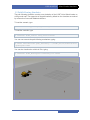
3.1 Driving Simulator
The driving simulation consists on a simulation of the L120F Volvo Whel Loader on the
Elkistsuna-Kjula map. You can also drive the vehicle and change the type of gravel pile on
the scenario using the keyboard.
To load the scenario type:
$ roslaunch l120f_gazebo l120f.launch
To load the L120F controller type:
$ roslaunch l120f_control l20f_control.launch
You can now execute the key_teleop.sh bash script and start driving the wheel loader.
$ cd ~/catkin/src/sim-control
$ ./key_teleop.sh
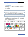
Once the key_teleop script is executed we can modify the velocity of the vehicle using the
keys W and S, change the direction of the vehicle using A and D, change the angle of the
laser using I and K, change the position of the bucket using U and J, moving up and down
the mechanical arm using O and L, change between the different models of piles using the
keys 1, 2 and 3, and stop the program using C.
7
USER MANUAL Wheel Loader Simulator
You can also visualize the vehicle in Rviz, typing:
$ roslaunch l120f_description l120f_rviz.launch
8
USER MANUAL Wheel Loader Simulator
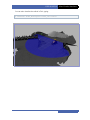
3.2 Path Following Simulator
The path following simulation consists on a simulation of the L120F Volvo Wheel Loader on
a flat ground map. The waypoints of the path loaded by default on the simulator are marked
by construction cones with disabled collisions.
To load the scenario, type:
$ roslaunch l120f_gazebo path_following.launch
To load the controller, type:
$ roslaunch l120f_control l20f_control.launch
You can now execute the path following mechanism, typing:
$ rosrun sim-controller path_following < ~/catkin_ws/src/simcontroller
/paths/path1.data
You can also visualize the vehicle in Rviz, typing:
$ roslaunch l120f_description l120f-mod_rviz.launch
9
USER MANUAL Wheel Loader Simulator
4. Technical details
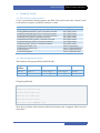
4.1 ROS-Gazebo communication
For the communication between gazebo and ROS some topics have been created. Is able
to subscribe to its topics or publish information on them.
Topic
Message
/l120f/leftRearWheelHinge_effort_controller/command
/l120f/rightRearWheelHinge_effort_controller/command
/l120f/leftFrontWheelHinge_effort_controller/command
/l120f/rightFrontWheelHinge_effort_controller/command
/l120f/steerJoint_position_controller/command
/l120f/cabinLaserJoint_position_controller/command
/l120f/ADLinkHinge_position_controller/command
/l120f/BuckHinge1_position_controller/command
/l120f/camera1/image_raw
/l120f/camera1/camera_info
/l120f/laser/scan
/l120f/odometry/data
std_msgs/Float64
std_msgs/Float64
std_msgs/Float64
std_msgs/Float64
std_msgs/Float64
std_msgs/Float64
std_msgs/Float64
std_msgs/Float64
sensor_msgs/Image
sensor_msgs/CameraInfo
sensor_msgs/LaserScan
sensor_msgs/Odometry
4.2 Path description file format
The format to the input path files should be like:
Waypoints
number
Rear X 1
Rear X 2
Rear Y 1
Rear Y 2
Front Angle 1
Front Angle 2
Pitch Angle 1
Pitch Angle 2
Effort 1
Effort 2
Example (path1.dat)
5
-20.0 6.0 -0.25 0.0 -2.0
0 26.0 -0.25 -0.80 -2.0
20.0 6.0 0.0 -2.88 -2.0
20.0 -20.0 0.0 0.0 10.0
0.0 -36.0 -0.25 -99999.0 -2.0
Note that a positive effort means backward movement and a negative effort forward
movement.
10
USER MANUAL Wheel Loader Simulator
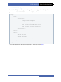
4.3 SickLMS200 Configuration
Inside the l120f.gazebo file you can change the laser configuration and adjust the
parameters of the SickLMS200 laser scanner. By default are:
<ray>
<scan>
<horizontal>
<samples>181</samples>
<resolution>1</resolution>
<min_angle>-1.570796</min_angle>
<max_angle>1.570796</max_angle>
</horizontal>
</scan>
<range>
<min>0.20</min>
<max>8.192</max>
<resolution>0.01</resolution>
</range>
</ray>
You can consult more information about the 1.4 SDF laser format here.
11