Download PowerDEVS. A Tool for Hybrid System Modeling and

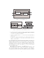
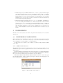
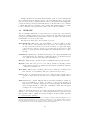
Submission for the Special Issue of Simulation: Software Tools,
Techniques and Architectures for Computer Simulation
PowerDEVS. A Tool for Hybrid System Modeling
and Real Time Simulation.
Federico Bergero† , Ernesto Kofman†
†Laboratorio de Sistemas Dinámicos. FCEIA - UNR. CIFASIS–CONICET.
Riobamba 245 bis - (2000) Rosario, Argentina
[email protected] [email protected]
Abstract
This paper introduces a general purpose software tool for DEVS modeling and simulation oriented to the simulation of hybrid systems. The
environment –called PowerDEVS - allows defining atomic DEVS models
in C++ language that can be then graphically coupled in hierarchical
block diagrams to create more complex systems. The environment automatically translates the graphically coupled models into a C++ code
which executes the simulation.
A remarkable feature of PowerDEVS is the possibility of performing simulations under a real–time operating system (RTAI) synchronizing
with a real time clock, which permits the design and automatic implementation of synchronous and asynchronous digital controllers. Combined with its continuous system simulation library, PowerDEVS is also
an efficient tool for real time simulation of physical systems.
Another feature is the interconnection between PowerDEVS and the
numerical package Scilab. PowerDEVS simulations can make use of Scilab
workspace variables and functions, and the results can be sent back to
Scilab for further processing and data analysis.
Besides describing the main features of the software tool, the article
also illustrates its use with some examples which show its simplicity and
efficiency.
Keywords: DEVS, Hybrid Systems, Real Time Simulation, Simulation
Software
1
INTRODUCTION
DEVS [32] is the most general formalism for discrete event system modeling.
It allows representing any system provided that it performs a finite number of
changes in finite intervals of time. Thus, not only Petri–Nets, State–charts,
Event–Graphs and other discrete event languages but also all discrete time
systems can be seen as particular cases of DEVS [30, 23].
1
Taking into account that ordinary differential equations can be approximated
by discrete time systems –using numerical integration methods– and that these
systems are particular cases of DEVS, it results that DEVS can also approximate
continuous systems. Moreover, there are numerical methods –like the Quantized
State System (QSS) family [4]– which produce simulation models that cannot
be represented in discrete time but only as DEVS models.
Thus, simulation tools based on DEVS are potentially more general than
tools for different discrete formalisms, including the popular continuous time
ones as Simulink [14] (Matlab), Scicos [3] (Scilab), etc.
Among the existing DEVS simulation tools we should mention DEVS–Java
[31], DEVSim++ [13], DEVS–C++ [6], CD++ [25] and JDEVS [7].
These software tools offer different features which include graphical interfaces and advanced simulation features for general purpose DEVS models and
for some specific domains. However, they were developed before the mentioned
discrete event methods for numerical integration of ordinary differential equations (ODEs).
These methods produce DEVS models with some very particular features on
one hand. In fact, they are usually composed of several atomic DEVS models
which belong to two basic classes: quantized integrators and static functions.
The different quantized integrators differ from each other in only two parameters: the quantum and the initial state value. Similarly, different static functions
only differ in some parameters as the gain, number of inputs, the calculated expression, etc.
On the other hand, these new numerical methods have many potential users
outside the DEVS–working community. In strongly discontinuous systems the
QSS methods offer solutions which are sensibly better than existing numerical
algorithms [18] and they are starting to be used by continuous system simulation
people. Unfortunately, most researchers and users of numerical ODE integration
methods do not know about DEVS and they would appreciate to use the DEVS–
based methods without learning DEVS. Moreover, they would be happier if the
software they have to use looks similar to the software they use for conventional
numerical methods (Simulink, Dymola, Scicos, etc.).
Taking into account these remarks, a DEVS simulation environment with library handling capabilities and a block–oriented graphical interface like Simulink
where parameters can be changed without modifying the blocks and where the
atomic DEVS definitions are hidden for non–DEVS–users appears as an appropriate solution for hybrid system simulation.
These ideas motivated the development of a general purpose DEVS simulation software oriented to hybrid system simulation. Here, we call hybrid system
any system involving simultaneous continuous (represented by ODEs) and discrete (represented by DEVS) dynamics.
This software package, called PowerDEVS was conceived to be used by
DEVS expert programmers as well as by end users who only want to connect
predefined blocks and simulate. The tool, initially developed as a Diploma Work
[22] in our University, was then re-written and is currently maintained by the
Laboratory for System Dynamics and Signal Processing.
PowerDEVS is composed of various independent programs:
• The Model Editor, which contains the graphical interface allowing the
hierarchical block-diagram construction, library managing, parameter se2
lection and other high level definitions as well as providing the linking
with the other programs.
• The Atomic Editor, which permits editing DEVS atomic models of elementary blocks by defining transition functions, output function, time
advance, etc.
• The Preprocessor, which translates the model editor files into structure
files which contain the coupling structure and the information to build
up the simulation code, links the code of the different atomic models
according to the corresponding structure file and compiles it to produce a
stand alone executable file which simulates the system.
• The Simulation Interface, which runs the stand alone executable and permits to vary simulation parameters such as final time, number of simulations to perform, and the simulation mode (normal simulation, timed
simulation, step-by-step simulation,etc).
• A running instance of Scilab, which acts as a workspace, where simulation
parameters can be read, and results can be exported to. This instance is
a modification of Scilab 4.1.2 to support this type of operations.
All these applications were programmed in C++ with the graphical libraries
QT, with the exception of the Model Editor that was programmed in Visual Basic. We provide compiled versions of these applications for Linux and Windows,
and all the source code is available for download too.
PowerDEVS also runs under a real time operating system (RTAI[19]) synchronizing the events with a real–time clock with the capability of capturing
interrupts at the atomic level. To this purpose, the DEVS simulation scheme of
[32] was partially inverted so that simulators of atomic models can send messages
to their parents informing about the next event time. In this way, PowerDEVS
allows the direct implementation of asynchronous DEVS–based Quantized State
Controllers [17] on a PC. Besides the Linux and Windows distributions, we developed a modified Kubuntu distribution that includes the RTAI kernel and
PowerDEVS.
The paper is organized as follows: Section 2 introduces the main concepts
used in the rest of the article. Then, Section 3 describes the main features
of PowerDEVS and Section 4 analyzes its real time characteristics. Finally,
Section 5 illustrates the usage of PowerDEVS in two examples (including a real
time control application) and Section 6 concludes the article.
2
2.1
BACKGROUND
DEVS
DEVS stands for Discrete EVent System specification, a formalism introduced
first by Bernard Zeigler [29].
A DEVS model processes an input event trajectory and –according to that
trajectory and its own initial conditions– it provokes an output event trajectory.
An atomic DEVS model is defined by the following structure:
M = (X, Y, S, δint , δext , λ, ta)
3
where:
• X is the set of input event values, i.e., the set of all possible values that
an input event can adopt.
• Y is the set of output event values.
• S is the set of state values.
• δint , δext , λ and ta are functions which define the system dynamics.
Each possible state s (s ∈ S) has an associated Time Advance computed by
the Time Advance Function ta(s) (ta(s) : S → ℜ+
0 ). The Time Advance is a
non-negative real number saying how long the system remains in a given state
in absence of input events.
Thus, if the state adopts the value s1 at time t1 , after ta(s1 ) units of time
(i.e. at time ta(s1 ) + t1 ) the system performs an internal transition going to
a new state s2 . The new state is calculated as s2 = δint (s1 ). Function δint
(δint : S → S) is called Internal Transition Function.
When the state goes from s1 to s2 an output event is produced with value
y1 = λ(s1 ). Function λ (λ : S → Y ) is called Output Function. In that way, the
functions ta, δint and λ define the autonomous behavior of a DEVS model.
When an input event arrives the state changes instantaneously. The new
state value depends not only on the input event value but also on the previous
state value and the elapsed time since the last transition. If the system arrived
to the state s2 at time t2 and then an input event arrives at time t2 +e with value
x1 , the new state is calculated as s3 = δext (s2 , e, x1 ) (note that ta(s2 ) > e). In
this case, we say that the system performs an external transition. Function δext
(δext : S × ℜ+
0 × X → S) is called External Transition Function. No output
event is produced during an external transition.
The formalism presented is also called Classic DEVS to distinguish it from
Parallel DEVS [32], which consists in an extension of the previous one conceived
to improve the treatment of simultaneous events.
Atomic DEVS models can be coupled. DEVS theory guarantees that the
coupling of atomic DEVS models defines new DEVS models (i.e. DEVS is
closed under coupling) and then complex systems can be represented by DEVS
in a hierarchical way [32].
Coupling in DEVS is usually represented through the use of input and output
ports. With these ports, the coupling of DEVS models becomes a simple block–
diagram construction. Figure 1 shows a coupled DEVS model N which is the
result of coupling the models Ma and Mb .
According to the closure property, the model N can be used itself as an
atomic DEVS and it can be coupled with other atomic or coupled models.
2.2
SIMULATING A DEVS MODEL
One of the most important features of DEVS is that very complex models can
be simulated in a very easy and efficient way.
The basic idea for the simulation of a coupled DEVS model can be described
by the following steps:
4
Ma
Mb
N
Figure 1: Coupled DEVS model
root − coordinator
coupled2
coupled1
atomic1
coordinator2
atomic2
atomic3
coordinator1
simulator1
simulator3
simulator2
Figure 2: Hierarchical model and simulation scheme
1. Look for the atomic model that, according to its time advance and elapsed
time, is the next to perform an internal transition. Call it d∗ and let tn
be the time of the mentioned transition.
2. Advance the simulation time t to t = tn and execute the internal transition
function of d∗ .
3. Propagate the output event produced by d∗ to all the atomic models connected to it executing the corresponding external transition functions.
Then, go back to step 1.
One of the simplest ways to implement these steps is writing a program with a
hierarchical structure equivalent to the hierarchical structure of the model to be
simulated. This is the method developed in [32] where a routine called DEVSsimulator is associated to each atomic DEVS model and a different routine
called DEVS-coordinator is related to each coupled DEVS model. At the top of
the hierarchy there is a routine called DEVS-root-coordinator which manages
the global simulation time.
Figure 2 illustrates this idea over a coupled DEVS model.
The simulators and coordinators of consecutive layers communicate with
each other with messages. The coordinators send messages to their children so
they execute the transition functions. When a simulator executes a transition,
it calculates its next state and –when the transition is internal– it sends the
5
output value to its parent coordinator. In all the cases, the simulator state will
coincide with its associated atomic DEVS model state.
When a coordinator executes a transition, it sends messages to some of its
children so they execute their corresponding transition functions. When an
output event produced by one of its children has to be propagated outside the
coupled model, the coordinator sends a message to its own parent coordinator
carrying the output value.
Each simulator or coordinator has a local variable tn which indicates the time
when its next internal transition will occur. In the simulators, that variable is
calculated using the time advance function of the corresponding atomic model.
In the coordinators, it is calculated as the minimum tn of their children. Thus,
the tn of the coordinator at the top is the time at which the next event of the
entire system will occur. Then, the root coordinator only looks at this time,
advances the global time t to this value and then it sends a message to its child
so it performs the next transition, and then it repeats this cycle until the end
of the simulation.
2.3
DEVS AND HYBRID SYSTEMS SIMULATION
Hybrid systems combine discrete and continuous dynamics. While discrete subsystems have a straightforward representation in DEVS, continuous submodels
require some type of discretization.
Although DEVS can easily represent the discrete time approximations of
continuous systems given by conventional numerical integration methods such
as Euler, Runge Kutta, etc., it can also represent the approximations resulting
from state quantization. Quantization based integration methods are noticeably
efficient to simulate hybrid systems due to their ability to handle discontinuities.
2.3.1
QUANTIZATION BASED INTEGRATION
Continuous time systems can be written as set of ordinary differential equations
(ODEs):
ẋ(t) = f (x(t), u(t))
(1)
where x ∈ ℜn is the state vector and u ∈ ℜm is a vector of known input
functions.
The simulation system (1) requires using numerical integration methods.
While conventional integration algorithms are based on time discretization, a
new family of numerical methods was developed based on state quantization [4].
The new algorithms, called Quantized State System methods (QSS methods),
can approximate ODEs like that of Eq.(1) by DEVS models.
Formally, the first order accurate QSS method approximates Eq.(1) by
ẋ(t) = f (q(t), v(t))
(2)
where each pair of variables qj and xj are related by a hysteretic quantization
function.
The presence of a hysteretic quantization function relating qj (t) and xj (t)
implies that qj (t) follows a piecewise constant trajectory that only changes when
the difference with xj (t) becomes equal to a parameter ∆qj called quantum.
6
The variables qj are called quantized variables, and can be seen as a piecewise
constant approximation of the corresponding state variables xj .
Similarly, the components of v(t) are piecewise constant approximations of
the corresponding components of u(t).
Since the components qj (t) and vj (t) follow piecewise constant trajectories, it
results that the state derivatives ẋj (t) also follow piecewise constant trajectories.
Then, the state variables xj (t) have piecewise linear evolutions.
Each component of Eq.(2) can be thought of as the coupling of two elementary subsystems, a static one,
ẋj (t) = fj (q1 , · · · , qn , v1 , · · · , vm )
(3)
Z
qj (t) = Qj (xj (·)) = Qj ( ẋj (τ )dτ )
(4)
and a dynamical one
where Qj is the hysteretic quantization function (it is not a function of the
instantaneous value xj (t), but a functional of the trajectory xj (·)).
Since the components vj (t), qj (t) and ẋj (t) are piecewise constant, both
subsystem have piecewise constant input and output trajectories that can be
represented by sequences of events.
Then, Subsystems (3) and (4) define a relation between their input and output sequences of events. Consequently, equivalent DEVS models can be found
for these systems, called static functions and quantized integrators, respectively
[4].
The piecewise constant input trajectories vj (t) can be also represented by
sequences of events, and source DEVS models that generate them can be easily
obtained.
Then, the QSS approximation Eq.(2) can be exactly simulated by a DEVS
model consisting in the coupling of n quantized integrators, n static functions
and m signal sources. The resulting coupled DEVS model looks identical to the
block diagram representation of the original system of Eq.(1).
Based on the idea of QSS, a second order accurate method was developed
replacing the piecewise constant approximations by piecewise linear ones. The
method, called QSS2, can be implemented using DEVS in the same way of
QSS. However, the trajectories are now piecewise linear instead of piecewise
constant. Thus, the events carry two numbers that indicate the initial value and
the slope of each segment. Also, the static functions and quantized integrators
are modified with respect to those of QSS so they can take into account the
slopes.
Following the idea of QSS2, the third order accurate QSS3 method [16] uses
piecewise parabolic trajectories. The family of QSS methods is completed with
three methods for stiff systems (Backward QSS and Linearly Implicit QSS of
order 1 and 2 [20]) and a method for marginally stable systems (Centered QSS
[5]).
2.3.2
QSS and HYBRID SYSTEMS
The interaction of the continuous and discrete dynamics occurring in hybrid
systems often implies that the right hand side of the system of Eq.(1) that
models the continuous subsystems contains discontinuities.
7
If a numerical integration method performs an integration step that crosses
through a discontinuity, the result will have an unacceptable error.
Conventional numerical methods solve this problem by finding the instant
of time at which the discontinuity occurs (this is usually called zero crossing).
Then, they advance the simulation up to that point, and they restart the integration from the new condition (after the event).
Although this idea works fine, it adds some computational cost: zero crossing
detection implies performing some iterations and the simulation restart can be
also quite expensive. Due to the presence of unbounded iterations, this solution
is usually unacceptable in the context of real time simulation [4].
Besides these difficulties, the simulation of a hybrid system requires also the
representation and simulation of the remaining discrete subsystems, which in
turn calls for the use of a common scheduling algorithm.
The usage of QSS methods on a DEVS simulation engine solves all the
mentioned problems. On one hand, DEVS provides the unified framework to
represent the discrete and the continuous (quantized) dynamics and to couple
them on a single model.
Also, according to the order of the QSS method used, the trajectories are
piecewise linear, parabolic or cubic. Thus, the zero crossing detection can be
analytically solved, without performing iterations at all.
Although the event associated to a discontinuity must occur at the right
time, the methods do not need to restart after that. After all, discontinuities in
QSS occur all the time, as the trajectories of qj (t) are discontinuous. Thus, for
the QSS approximations, a discontinuity has the same effect of a normal step.
Moreover, when a component fj of the system (1) contains a discontinuity,
the DEVS static function computing ẋj (t) will be in charge of detecting the
discontinuity and provoking the right event trajectory for the state derivative.
In other words, discontinuities are detected and handled locally, without any
additional computational cost for the rest of the simulation.
These advantages result in a noticeable simulation speedup with respect to
conventional numerical algorithms. In models with rapidly occurring discontinuities such as power electronic systems, the high order QSS2 and QSS3 and
LIQSS2 can perform simulations up to 20 times faster than all existing conventional methods [18].
2.4
SIMILAR TOOLS
There is a great variety of tools in the field of DEVS simulation. Some are plain
DEVS simulators, without real time support, and others are general continuous
system simulation tools. Here we describe a few of these tools.
• ADEVS [21] is a C++ library to simulate DEVS based models. Unlike
PowerDEVS it is based on two DEVS formalism extensions, called Parallel
DEVS and Dynamic DEVS which treat simultaneous events in a different
way (confluent transition). ADEVS is a library, but it does not have a GUI
for model coupling and the model has to be described alphanumerically.
• CD++[24] is a DEVS simulation tool developed by Gabriel Wainer’s
group. It is based on another DEVS extension, called Cell-DEVS, which
merges DEVS and cellular automata. It has support for real time simulation.
8
• DEVSJava[32, 11] is a DEVS simulation tool developed by Bernard Zeigler
and Hessam Sarjoughian. It has interesting features such as changing
the model structure at run time (or simulation time). Also, it offers a
hierarchical view of the model structure. It has support for real time
simulation in a best shot way, because it is written in Java and runs under
non-real-time Operating Systems.
• Matlab Real Time Workshop[12] is a toolbox of Simulink. Simulink is a
tool for modeling and simulation of continuous systems. It has a GUI in
which models can be described in a Block Diagram fashion. It supports
generating C++ code for running the simulation under a variety of RTOS.
The Real Time Workshop (being a part of Matlab) is a proprietary software of The MathWorks and its use and distribution is restricted by its
license.
3
POWERDEVS
In this section we describe the main components and features of the software
developed.
3.1
POWERDEVS COMPONENTS
As we mentioned, PowerDEVS is composed of various independent programs:
the model editor, the atomic editor, the preprocessor and the simulation interface
and a workspace corresponding to a Scilab instance.
In this section we describe each of this tools and how they interact which
each other.
3.1.1
THE MODEL EDITOR
The Model Editor is –from a user point of view– the main program of PowerDEVS as it provides the graphical interface and the link with the rest of the
applications.
Besides building and managing models and libraries, it permits launching a
simulation (by invoking the Preprocessor) and editing elementary blocks up to
the atomic model definitions (by invoking the Atomic Editor).
The Model Editor main window (Fig. 3) allows the user to create and open
models and libraries. It also permits exploring the libraries and dragging blocks
from the libraries to the models.
Figure 3: Model Editor main window.
9
There are also some advanced features which can be managed from the main
window like setting which are the active libraries (i.e. which libraries are shown
when exploring), and configuring the tool bars and menu to invoke new external
applications.
Models and libraries can be edited in a model window with the open and
new model commands. Figure 4 shows a model window with a model composed
by five sub–models.
Figure 4: Model Window.
The Model Windows provide all the typical graphical edition facilities so
that blocks can be copied, resized, rotated, etc. while the connections can be
directly drawn between different ports.
From the edit menu (or with the right button) it is possible to edit the
features of each block, no matter if it corresponds to a coupled or an atomic
model.
The Block Edition Window (Fig. 5) allows to configure the graphic appearance of the block, to choose the block parameters and –in the case of atomic
models– to select the file which contains the associated code with the DEVS
model definitions.
The block parameters are defined and selected in the block edition windows.
After being defined, their values can be changed by double–clicking on the block
(Fig. 6). Thus, when we take predefined blocks from the libraries, we can change
the parameter values without editing them. As we shall see in Section 3.1.3,
the values of these parameters are passed to the corresponding DEVS atomic
or coupled models.
Coupled models do not have an associated code, but they have some extra
features which can be modified from the block edition window and the edit
menu (the internal priorities and the order of the input and output ports, for
instance).
10
Figure 5: Block Edition Window.
Figure 6: Changing parameter values.
3.1.2
THE ATOMIC EDITOR
The Atomic Editor facilitates the edition of the C++ code corresponding to
each atomic DEVS model.
It can be invoked from the Block Edition Window to edit an existing code
or to create a new one. It can be also run directly from the OS since it is a
stand alone application. The Atomic Editor main window is shown in Figure 7.
Using the atomic editor, the user only has to define the variables which form
the state and the output of the DEVS model and the variables which represent
the parameters of the system. After that, the C++ code of the time advance,
transition and output functions must be placed in the corresponding windows.
There are two additional windows (init and exit) where the user can also add a
piece of code that is executed before the simulation starts (to set initial states
and parameters, for instance) and a piece of code that is executed at the end of
the simulation (to close some open files, for instance). When the model is saved,
the code is automatically completed and stored in the corresponding .cpp and
11
Figure 7: Atomic Editor main window.
.h files.
Besides facilitating the programming, the Atomic Editor was designed to give
the user the possibility of writing a code which is very similar to the DEVS model
definition. All the rest of the job –related to simulation and implementation
issues– is automatically performed by the program.
Let us illustrate this fact with a simple DEVS model. Consider for instance
a system which calculates a static function f (u0 , u1 ) = u0 − u1 with u0 and u1
being real-valued piecewise constant trajectories. If we represent those trajectories by sequences of events –as it is done in QSS–methods– we can build the
following atomic DEVS model:
M = (X, Y, S, δint , δext , λ, ta), where
S = ℜ 2 × ℜ+
δint (s) = δint (u0 , u1 , σ) = (u0 , u1 , ∞)
δext (s, e, x) = δext (u0 , u1 , σ, e, xv , p) = s̃
λ(s) = λ(u0 , u1 , σ) = (u0 − u1 , 0)
ta(s) = ta(u0 , u1 , σ) = σ
with
s̃ =
(xv , u1 , 0) if p = 0
(u0 , xv , 0) otherwise
We use integer numbers from 0 to n − 1 to denote the input and output ports
(because PowerDEVS does so).
This DEVS model translated into PowerDEVS has the following code (at
the Atomic Editor Fig. 7):
ATOMIC MODEL STATIC1
State Variables and Parameters:
12
float u[2],sigma; //states
float y; //output
float inf ; //parameter
Init Function:
inf = 1e10;
u[0] = 0;
u[1] = 0;
sigma = inf ;
y = 0;
Time Advance Function:
return sigma;
Internal Transition Function:
sigma=inf ;
External Transition Function:
float xv;
xv=*(float*)(x.value);
u[x.port] = xv;
sigma = 0;
Output Function:
y = u[0] − u[1];
return Event(&y,0);
It is clear that the translation from the atomic DEVS into the PowerDEVS code
is almost straightforward.
With that code, the Atomic Editor automatically produces the .cpp and .h
files which are then used by the Preprocessor to generate the simulation of the
whole system.
3.1.3
THE PREPROCESSOR
The Preprocessor takes a .pdm (or .pds) file produced by the model editor and
produces the simulation program.
It basically translates the .pdm file into a header .h file (called model.h)
which binds the simulators and coordinators according to the coupling structure
passing also the block parameters.
The preprocessor also produces a makefile (Makefile.include) which is then
invoked to compile and generate the program which implements the simulation
(that program is called model).
As we mentioned before, the Preprocessor can be invoked in a transparent
way using the Quick Simulation command. Anyway, it can be also called from
the command line (it is also a stand alone application).
3.1.4
THE SIMULATION INTERFACE
The generated program model, when executed, simulates the associated DEVS
model.
PowerDEVS provides a graphical interface for running the simulation (Fig. 8).
The interface also allows to change some parameters to set up the experiment:
• Final Time: tells for how long to simulate the model.
13
Figure 8: Simulation Interface
• Simulations to run: multiple simulation runs can be executed at once. This
can be useful when statistics from simulation results are to be calculated.
• Illegitimate check break: PowerDEVS stops the simulation if the time
does not advance after a selected number of steps. This avoids hang-ups
in illegitimate models.
• Simulate step-by-step: the simulation can be advanced performing one
step (or many) at the time, and results can be analyzed in between.
• Synchronize time: The simulation can be run synchronized with the real
clock (with the precision of the underlying OS).
Also, the model program can be invoked from the command line, and executed in an interactive shell. All the simulation parameters can be changed in
the same way they are changed from the graphical interface.
3.2
INTERNAL IMPLEMENTATION
Having described the main functional aspects of PowerDEVS, we shall now
explain the way in which the simulation algorithm described in Section 2.2 is
implemented inside the program that executes the simulation.
As PowerDEVS performs an object oriented simulation, we shall start describing the internal class structure.
Atomic models with the same associated code belong to a particular class
(defined by that code). For instance, the Integrator atomic models in the model
of Fig. 4 belong to the Integrator class, defined in the files integrator.h and
integrator.cpp which contain the code associated to that atomic model.
14
When the code of an atomic model is written using the Atomic Editor, the
code related to the class definition is automatically generated.
All the atomic classes are derived from the simulator class. The simulator
class is an abstract class which acts as an interface to deal with different atomic
model implementations. The variables representing the state of the model and
the functions that operate on it (time advance, transition and output functions)
are member variables and methods.
The external transition and output functions of the simulator class receive
and return respectively objects belonging to the Event class. Events have the
following properties:
• Event.port: is an integer number indicating the input or output port where
the event is received or sent.
• Event.value: is a pointer to void. That way, the values carried by the
events can belong to arbitrary types.
• Event.realTimeMode: is an integer that can take the following values: 0
(indicating that the event is not synchronized with the real time), 1 (with
normal synchronization) and 2 (with precise synchronization). When an
event has its mode set to 1 or 2 (the difference between them will be
explained in Section 4.2.1), the simulation engine waits until the physical
time reaches the simulation time to propagate it.
To provide the capability of initializing and stopping devices that interact
with the hardware, the simulator class has two extra methods which are not
included in the definition of [32]. As we already mentioned, for real–time simulation purposes PowerDEVS also inverts the time managing features. Thus,
when an atomic model receives an interrupt request from an external device, it
informs the change in its time to next event (tn) to its parent.
The hierarchical coupling structure is implemented by the coupling class.
This class is similar to the coordinator in Fig. 2. Each object of this class is
associated to a coupled DEVS model and it contains a list of references to the
corresponding connections, atomic and coupled models.
The difference with the coordinator is that, following the simulator class
behavior, the coupling objects are able to receive the messages coming from
their children notifying changes in their time to next event. Similarly, the
coupling objects have also the possibility of informing their own parent about
changes in their tn. Coherently with the closure property, the coupling class is
derived from the simulator class.
The coupling and simulator objects also contain objects belonging to the
classes connection and event (the first one is only in the coupling class). The
connection class is formed by four integer numbers representing two pairs of
models and ports. The event objects are formed by a pointer to void and an
integer (identifying the input or output port). Thus PowerDEVS models can
produce output events which belong to different types.
Having defined the model structure in terms of components and functionality, we shall now describe the framework developed to actually execute the
simulation.
The root–simulator class is in charge of running the simulation. Basically,
this class manages the simulation advance interacting with the object represent15
ing the coupling at the top of the structure. Thus, the root–simulator plays the
role of the root–coordinator in Fig. 2.
Before following the description we should mention that the behavior of the
top coupling object has a small difference with the others. In terms of the
simulation execution, there is no coupling above to notify the timing changes
but these changes should be notified directly to the root–simulator. Thus, a new
class denominated root–coupling has been introduced. This class, derived from
the coupling class, has the same functionality as the latter but it differs in the
hierarchical superior object.
Finally, the main class of the simulation program is called model. This
class provides the interactive shell for interacting with the user (or with the
graphical simulation interface of Fig.8 ) and running the simulation. This class
talks directly with the root–simulator allowing the user to start the simulation
in different modes.
The objects which form the coupling structure are instantiated at the model.h
file. This file is automatically generated by the Preprocessor and it declares the
simulators, couplings and connections according to the structure file.
In fact, the only difference between the codes that execute the simulation
of two different models is in that file (model.h). Obviously, the fact that both
files are different also implies that they may include different simulators corresponding to different atomic models.
3.3
INTERCONNECTION WITH SCILAB
Scilab [8] is a numerical computational package developed by the Institut National de Recherche en Informatique et Automatique (INRIA) and it is released
under the GPL license. Scilab is an Open Source alternative to the widely used
software Matlab.
Scilab contains an interactive interface where the user can define variables
and matrices and perform complex operations between them. It also has a
programming language that can be used to define new functions and algorithms,
and some graphical tools to plot data. The Scilab distribution includes several
toolboxes (i.e., set of functions developed by different people) to solve problems
related to Linear Algebra, Signal Processing, Automatic Control, Optimization,
Filtering Design, etc.
To make the communication between PowerDEVS and Scilab, some modifications to the source code of Scilab were made. These modifications open
a ”back door” into Scilab’s workspace, where variables can be read or written
from PowerDEVS .The communication is performed through UDP messages
over the port 27015 in a client–server model, with Scilab acting as server and
PowerDEVS as client.
3.3.1
THE SCILAB SIDE
As Scilab is an open-source tool, all its source code is available online to view,
edit and enhance. We used Scilab 4.1.2 version and made modifications in both,
Linux and Windows source versions. These modifications were made in the files
routines/wsci/WScilex/WScilex.c (for Windows) and routines/xsci/x_main.c
(for Linux).
16
As the idea was to use Scilab as PowerDEVS workspace –that is, PowerDEVS runs the simulation and Scilab responds to PowerDEVS commands–
it was necessary to modify the normal behavior of Scilab in order to establish
the communication.
To keep running the Scilab GUI, while communicating with PowerDEVS a
new thread is created in Scilab address space. This new thread is in charge of
receiving, executing, and responding to PowerDEVS requests.
The actual communication between PowerDEVS and this Scilab thread was
implemented in a Client-Server model over UDP. Under this architecture, Scilab
(acting as the server) waits for requests on the UDP port 27015 and PowerDEVS
sends requests to that port (see Fig. 9).
Figure 9: PowerDEVS –Scilab communication
The PowerDEVS requests sent to Scilab consist of string representations
of the commands to execute in Scilab workspace (for example “freq=pi*345”).
Each request starts with a character indicating if Scilab must notify PowerDEVS
once the command execution is finished.
The Scilab notification to PowerDEVS (when the first character indicates
so) consists of a UDP message containing the value of the “ans” variable in
Siclab workspace. This permits –indirectly– to evaluate any Scilab expression
or variable from PowerDEVS sending the correct command sequence.
3.3.2
THE PowerDEVS SIDE
The PowerDEVS simulation engine has a set of services to communicate with
Scilab. These services can be called from any atomic model written with the
atomic editor:
void getAns(double *ans, int r, int c);
void putScilabVar(char *varname, double v);
double getScilabVar(char *varname);
double executeScilabJob(char *job, bool blocking);
The function getAns(double *ans, int r, int c) returns the answer of
the last calculation in the Scilab workspace (i.e., the “ans” variable). The result
is put in the double pointed by ans. The r and c arguments indicate the
size of the result to be retrieved (Scilab works with matrices and so does the
PowerDEVS interface). If a scalar value is to be retrieved r and c must be 1.
The functions putScilabVar(char *varname, double v) and
getScilabVar(char *varname) are the basic methods to interact with Scilab
variables. putScilabVar creates (or updates) the Scilab variables named varname
with value v. On the other hand, getScilabVar reads the variable named
varname from Scilab workspace. If the variable does not exist this function
returns 0.0 and writes a warning message in the simulation log.
17
Finally, the function executeScilabJob(char *job, bool blocking) runs
the command job in the Scilab workspace. It works just like when one types the
sentence in the Scilab command window. The second argument blocking indicates if the function should return immediately or should wait for the command
to finish. The function returns the “ans” variable (like getAns) which –according
to the command– can represent the result of the executed command.
3.4
LIBRARY
The PowerDEVS distribution comes with a set of atomic and coupled models
already programmed, that can be used to build new models. These basic models
form the PowerDEVS library (any advanced user can easily extend the library
including his own developed models).
The library is divided into the following categories:
Basic Elements: This is the only PowerDEVS core library. Based on these
models, all the other libraries where developed. It contains four basic
models, an atomic (a skeleton for all the atomics), a coupled (an empty
coupled model), and two special objects called inport and outport. The
last two objects represent external input and output interfaces for coupled
models.
Continuous: This library contains models that process continuous signals based
on the QSS methods to simulate continuous systems1 . It includes integrators, gains, non–linear static functions, multipliers, etc.
Discrete: This library contains models for simulating discrete time systems.
Hybrid: Under this category, a set of models are included combining continuous and discrete features to simulate hybrid systems: quantizers, switches,
comparators, samplers, etc.
Real Time: This library contains specific blocks to make use of different real
time features of PowerDEVS . They are described in Section 4.3.
Source: Here we can find several sources for continuous time signals approximated by QSS methods, like sine waves, ramps, pulses, square waves,
etc.
Sink: This library contains different sink models where simulation results are
sent for visualization or future processing. Some models included in
this library are: GnuPlot (which plots its input signals), ToDisk (which
writes its input signals to a CVS file), toWorkspace (that writes in Scilab
workspace the received signal), etc.
All the models in the library accept Scilab expressions as parameter values. For
instance, one could use “freq*2+0.5” as the gain parameter in a gain block, and
this expression will be evaluated in Scilab workspace (in this example freq must
be a defined Scilab variable).
1 The Continuous library was conceived to simulate Ordinary Differential Equations. Differential Algebraic Equations can be simulated with the use of the Implicit Function Block,
that implements the methodology developed in [15]. If instead of using that block an algebraic
loop is included in the model, the simulation will result illegitimate.
18
4
POWERDEVS IN REALTIME
As we anticipated earlier, PowerDEVS was extended to run on a real time
operating system. For some reasons that will be explained soon in this section,
we choose Linux RTAI as the RTOS for PowerDEVS .
The simulation engine of PowerDEVS is an implementation in C++ of the
simulator decribed in Section 2.2. As RTAI is an extension of Linux, in principle,
the PowerDEVS simulations (that run fine under Linux) should also run under
RTAI.
Although this is true, the goal of running a simulation under RTAI is making
use of its services to ensure real time perfomance. So several modifications were
made in the PowerDEVS simulation engine which enable the user to easily
access basic services like synchronizing events, capturing and handling hardware
interrupts, obtaining file support and performing real time measurement.
Also, the PowerDEVS library was extended with a set of blocks to make use
of these services in a simple drag-and-drop way.
This section, after introducing some concepts related to real time systems
and real time simulation, describes the extensions made to the simulation engine, the new library blocks and some experiments done to measure different
performance indicators of PowerDEVS in real time.
4.1
4.1.1
REAL–TIME SYSTEMS & RTOS
REAL–TIME SYSTEMS
A real–time system is a system in which computations are subject to real–time
constrains. That is, responses to stimuli have a dead-line that must be met,
regardless of system load, in order for the system to be considered correct.
Real–Time systems can be classified in two categories:
Hard real time systems: in which the completion of a computation after its
deadline is considered useless, and may cause critical failures in the system.
Soft real–time systems: in which a missed deadline can be accepted, or ignored or even corrected.
4.1.2
REAL–TIME OPERATING SYSTEMS (RTOS)
Real-Time Operating Systems (RTOS) are a special class of Operating Systems
(OS) which provide the basic tools and services to implement systems with time
constraints.
This kind of OS should be expressive enough to represent the time constraints
of each task, the way these tasks communicate, and must have some control over
the low-level hardware of the computer (memory, interrupts, ports).
Some commonly used RTOS are QNX [10], VxWorks [26], Drops [9], RTLinux [1], RTAI [19], etc..
Among them, we decided working using RTAI (RealTime Application Interface) because it consists of an extension of the Linux Kernel [2] that permits
running all the software that runs on Linux. This was a crucial requirement in
the context of this work since we wanted to run not only PowerDEVS, but also
the external applications that communicate with it (GNUPlot and Scilab).
19
Also, the fact that RTAI is distributed under the GPL License allows us
to freely distribute the real time version of PowerDEVS included with the OS
installer.
4.1.3
RTAI
RTAI is a RTOS that supports several architectures (i386, PowerPC, ARM).
RTAI is an extension of the Linux kernel to support real time tasks to run
concurrently with Linux processes. This extension uses a method to enable
this, first used in RT-Linux [1].
Linux kernel is not itself a RTOS. It does not provide real time services, and
in some parts of the kernel, interrupts are disabled as a method of synchronization (to update internal structures in an atomic way). These periods of time
where interrupts are disabled, lead to a scenario where the response time of the
system is unknown, and time deadlines could be missed.
To avoid this problem RTAI inserts an abstraction layer beneath the Linux
kernel. In this way, Linux never disables the real hardware interrupts. The
Linux kernel is run under another micro-kernel (RTAI + Adeos 2 ) as user processes. All hardware interrupts are captured by this micro-kernel and forwarded
to Linux (if Linux has interrupts enabled).
Another problem running real time tasks under Linux is that the Linux
scheduler can take control of the processor from any running process without
restrictions. This is unacceptable in a real time system. Thus, in RTAI real time
tasks are run in the micro-kernel, without any supervision of Linux. Moreover,
these processes are not seen by the Linux scheduler.
Real time tasks are manged by the RTAI scheduler. Clearly, there are two
different kinds of running processes, Linux processes and RTAI processes. RTAI
processes cannot make use of Linux services (such as File system) and vice versa.
To avoid this problem, RTAI offers various IPC mechanisms (Pipes, Mailboxes,
Shared Memory, etc.).
RTAI provides the user with some basic services to implement real-time
systems:
Deterministic interrupt response time: An interrupt is an external event
to the system. The response time to this event varies from computer to
computer, but RTAI guarantees a boundary (on each computer), which
is necessary to communicate with external hardware, for example a data
acquisition board.
Inter Process Communication (IPC): RTAI offers various methods of IPC,
such as semaphore, pipes, mailbox and shared memory. These IPC mechanisms can be used to connect processes running in real time with normal
Linux processes or vice versa.
High precision timers: When developing real time systems, the time handling accuracy is very important. RTAI offers clocks and timers with ns
(1e−9 s) precision. On i386 architectures, these timers use the processor’s
time stamp, therefore, they are very precise.
2 Adeos [27, 28] is the abstraction layer used in RTAI. Adeos implements the concept of
interrupt domain. http://home.gna.org/adeos/
20
Interrupt Handling RTAI allows the user to capture hardware interrupts and
treat them with custom user handlers. Normal Operating Systems (such
as Linux, Windows) hide hardware interrupts from the user, making the
development of communication with external hardware a bit more difficult
(you have to write a kernel driver). As said before, the response time is
bounded.
RTAI tasks can be run in two different modes
Loadable kernel module: in this mode executable files are not stand alone
programs but loadable kernel modules. The RTAI process is inserted in
the running Linux kernel and from then on it switches to the RTAI scheduler. Running in kernel mode (as modules do) gives the process certain
privileges and rights that normal user processes do not have (accessing
kernel objects, writing/reading ports, etc).
LXRT: RTAI offers a library called LXRT for developing real time systems
in user space. LXRT is a “bridge” between Linux user mode and RTAI.
LXRT brings to the user space all RTAI services. LXRT works with
a concept called angel process. LXRT creates a RTAI counterpart (the
angel process) in charge of executing all the real time services on behalf
of the user space process.
Having described the main features of RTAI, we shall now focus on the
extensions made to PowerDEVS .
4.2
PowerDEVS ENGINE SUPPORT
Four new modules were added to the simulation engine to make use of the real
time services provided by RTAI. The modules consist in new functions that can
be used by any atomic model.
4.2.1
SYNCHRONIZATION MODULE
This module is the cornerstone of PowerDEVS in real time. It allows the
simulation engine to synchronize the events with the RTAI real clock.
RTAI has two methods of synchronizing, both with ns precision:
• rt sleep: waits for an amount of time, releasing the processor.
• rt busy sleep: waits for an amount of time by busy-waiting, that is, burning
CPU cycles until the wait is over. In this mode, a more precise synchronization is obtained.
Based on these two methods, the PowerDEVS simulation engine implements
the function waitFor(unsigned long int nanoseconds, int mode) which waits
the specified time in one of two modes: Normal or Precise.
This function has the following logic:
• If the amount of time to wait is too small (smaller than a constant that
defines the synchronization accuracy), the sentence is ignored.
• If the function is called in Normal mode, the non–busy rt sleep is invoked
(where the CPU is released).
21
• If the function is called in Precise mode, the beahvior depends on the time
to wait:
– If the period is less that a given constant (which defines the accuracy of the non–busy rt sleep), a busy waiting is performed invoking
rt busy sleep.
– Otherwise, the waiting is split in two periods. The first period is
computed as the whole period minus twice the non–busy accuracy,
and it is performed in a non–busy way invoking rt sleep. After finishing this period, the time is measured again (to eliminate the error
introduced by the non–busy waiting) and the remaining waiting time
is done with a busy–waiting. This way, the synchronization has the
accuracy of a busy waiting, but the processor is released most of the
time.
The function waitFor can be invoked by any atomic model, but it is automatically called by the simulation engine when an output event has its realTimeMode property (see Section 3.2) set to 1 or 2.
This way, in the same model, some events can be propagated immediately
(when their realTimeMode is set to 0) and others can be synchronized either in
normal or precise mode. This gives the user the possibility of choosing which
events must be synchronized (typically those that involve communication with
external hardware) and which should be computed as fast as possible (those
involving intermediate calculations).
4.2.2
INTERRUPT HANDLING MODULE
This module is in charge of managing the interaction between the PowerDEVS
simulation engine and the hardware interrupts.
Any atomic can express interest in a specific hardware interrupt by calling:
requestIRQ(int irq);
When a hardware interrupt irq occurs, the simulation engine sends an external transition message to all the atomic models that have expressed interest
in that interrupt. The message arrives to a non–exisiting port (denoted -1).
Since these atomic models will possibly change their time advances in the
external transition, the engine automatically transmits from the bottom to the
top of the hierarchy about these changes. This is the mechanism that we mentioned in Section 2.2, and it is the only modification of the abstract simulator
of [32] introduced by PowerDEVS .
4.2.3
FILE SUPPORT MODULE
When a task is running under RTAI, it can not make use of Linux services (such
as Linux File System). This is because a system call to the Linux kernel does
not have a deterministic response time, so, a system call could lead to missing a
deadline in the real time system. In fact, RTAI tasks are not scheduled by the
Linux scheduler which does not know they exist. Thus, to enable the simulations
to use files, a File Support Module was developed. This module has two parts:
22
Real Time Interface: It is a real time task (running under RTAI) that accepts
the requests of the real time simulation (like open, read, write files). It
communicates with a program running under Linux user space (which has
access to the Linux File System) using a Real Time FIFO (one of the IPC
provided by RTAI).
User space Angel: It is a normal Linux program that accepts commands from
the Real Time Interface. This program (which is launched together with
the simulation) makes all the system calls on behalf of the simulation.
The interface provides similar functions to those of the c library (stdio) that
can be directly used by any atomic model.
4.2.4
REALTIME MEASUREMENT MODULE
This module allows the atomics models to ask for the value of the real time
clock. This is useful, for instance, when a user wants to change the behaviour of
an atomic model depending on the difference (in either way) between the real
time and the simulated time (to handle overruns or to compute more precisely
if enough time is available).
4.3
REALTIME LIBRARY
To make use of all the real time features in a simple way, the PowerDEVS library
was extended to include several atomic blocks that can be included directly in
the models.
RTWait: This atomic block receives events and outputs them synchronized
with the real time clock. In this way, a normal model (i.e. non–real time)
can be transformed into a real time model by inserting these blocks on
the connections carrying events that need to be synchronized. The block
has a parameter to choose what kind of synchronization must be made,
precise or normal (see 4.2.1).
RTClock: When this block receives an event (no matter what the value of
the event is), it emits an event whose value is equal to the real time clock
value.
ToDisk: This model writes the input signal in a CSV(Comma Separated Values) file. It makes use of the File Support Module to run in real time.
IRQDetector: This model is the user interface for the Interrupt Handling
Module. It emits an event whenever the hardware interrupt occurs. From
the point of view of the DEVS formalism (and from PowerDEVS too)
this is a passive model (its time advance is ∞), but when the associated
interrupt is triggered, the model changes its own time advance to 0 (and
the engine automatically notifies its parent of this change). The block has
a parameter to indicate which interrupt it waits for.
23
4.4
REAL TIME PERFORMANCE
One of the most important features to characterize a real time system is the
error (or latency) of synchronization.
We conducted several experiments to see how the system responds (in relationship to the load of the system). All the experiments where run on a PC
AMD Athlon 1.8 GHz.
First, we did the following experiment: we simulated a source block which
generates a QSS-approximation of a sine wave at 440Hz (this model generates
20 events per cycle, to a total of 8800 events per second). The model was
simulated in real time measuring the maximum and average latency. Also the
two different modes (see Sect. 4.2.1) of waiting were tested. The following
results were obtained:
Wait
Normal
Precise
Table 1: Synchronization error with low load
Maximum Average Overruns
4800 ns
1500 ns
450 ns
180 ns
-
Next, a simulation of a more complex model was performed: a PI control
of a DC motor using Pulse With Modulation (PWM). In this example, several
simulations were run varying the PWM carrier from 1000 to 20000 Hz:
f (Hz)
1000
15000
17000
20000
Table 2: Synchronization error with varying load
Wait Mode Maximum Average.
Overruns
Normal
5786 ns
1512 ns
Precise
1330 ns
180 ns
Normal
5622 ns
1622 ns
372 / 19905 ev.
Precise
1000 ns
512 ns
305 / 19905 ev.
Normal
4547 ns
1648 ns
6119 / 17616 ev.
Precise
973 ns
454 ns
5924 / 17616 ev.
Normal
0 ns
0 ns
18292 / 18292 ev.
Precise
0 ns
0 ns
18292 / 18292 ev.
As can be seen in table 2, using a frequency of 1000 Hz there are no overruns.
With frequencies between 15000 Hz and 17000 Hz, there are more overruns and
the Linux system (not the real-time system) experiences some delays, which
indicates that the system load is high.
With a frequency of 20000 Hz the system stops responding (the Linux part)
and we see that all events are emitted after their time deadline.
This last case reflects a limitation of the hardware platform, not a limitation
of the system synchronization. What happens with a frequency of 20000Hz is
that the hardware cannot complete the calculations in time.
24
4.5
INTERRUPT LATENCY
To measure the interrupt latency the following procedure was used.
A PowerDEVS model was created (Fig. 10) which generates hardware interrupts and then captures back these interrupts, measuring the period of time
between the generation of the signal provoking the interrupt and the capture of
the interrupt by the handler.
For that purpose, we used the PC Parallel port. One of the pins on the
parallel port (STO) is in charge of generating interrupts. This pin was wired to
a data pin, thus generating a hardware interrupt every time that the data pin
goes from a low state (0 V) to a high state (5V). The model stores the time
at which a 1 is written to the data pin (high state), and the time at which the
interrupt handler of the parallel port is run. The difference between these two
times is an upper bound of the interrupt latency of the system (in fact, that
difference includes also the time needed to write on the parallel port and the
electrical transients).
Figure 10: Interrupt Latency tester model
Running this experiment on the same hardware (PC AMD 1.8Ghz) we obtained an upper bound on the interrupt latency of about 20µs.
5
EXAMPLES
This section describes two examples that show different features of PowerDEVS.
5.1
RIPPLE VS FREQUENCY IN A BUCK CIRCUIT
Figure 11 represents a DC-DC converter circuit known as Buck Circuit.
The presence of the switch introduces hybrid behavior to the system.
The goal of the experiments is to analyze the dependence of the ripple amplitude on the switching frequency. In this example we used the following parameters L1 = L2 = 0.1mH, C = 20µF, Rl = 10Ω and U = 12V.
Figure 12 shows the PowerDEVS model of the circuit, made entirely with
atomic blocks from the PowerDEVS library. The switch is commanded by a
25
L1
L2
+
C
U
Rl
-
Figure 11: Buck Circuit
PWM signal. The remaining blocks implement source, static functions and
integrators based on QSS methods.
The frequency of the triangular carrier was chosen in a way that increments
2000Hz in each simulation. The “RunScilab Job” block increments the Scilab
variable n after each simulation and calculates the ripple amplitude in steady
state. This amplitude is saved in the array u(n).
Figure 12: Buck Circuit Model
After 100 simulations (in which the frequency goes from 2000 to 200000 Hz),
we can plot the results directly in Scilab (see Fig. 13).
It must be noticed that 100 simulations of this hybrid system (with very quick
commutations) were run, and thanks to the efficiency of the QSS methods to
treat this kind of problems, the experiment only took about 13 seconds (while
in Matlab/Simulink it takes about a minute).
26
Figure 13: Ripple vs. Frequency
5.2
DC MOTOR CONTROL IN REALTIME
This example shows the real time asynchronous control of a DC Motor. For this
purpose, we used a small DC drive moving an old PC mouse wheel acting as an
encoder (see Fig.14). Each time the wheel moves a small angle, a pulse is sent
to the bit STO of the parallel port, which triggers an interrupt in the PC. The
motor is fed by an amplifier, implemented with a transistor and a filter taking
the on–off voltage from a data pin of the parallel port.
Figure 14: Motor and mouse (encoder)
The control system is composed of the following subsystems (see Fig. 15):
• The Motor Speed block detects and counts the interrupts generated by the
encoder to estimate the motor speed.
27
• This estimation is compared to the reference speed (the block WSum4
calculates the difference or error).
• In base of this error a Proportional-Integral (PI) Control is applied, using
QSS discretization.
• The control signal (previously saturated to avoid over-modulation) is pulse
width modulated.
• The PWM signal (calculated in the Comparator1 block), is sent syncronized to the parallel port.
Figure 15: Proportional Control Model
The whole control system of Fig.15 was built using blocks from the PowerDEVS library, except the model that estimates the motor speed based on the
number of interrupts it receives per second.
Figure 16 shows the reference speed signal while Fig. 17 shows the speed
measured by the control system.
90
80
70
60
50
40
30
20
10
0
-10
0
2
4
6
8
10
Figure 16: Reference speed
6
CONCLUSIONS AND FUTURE WORK
We introduced and described a general purpose tool for DEVS simulation. We
illustrated its use in hybrid system simulation, where it shows the most impor28
80
70
60
50
40
30
20
10
0
0
2
4
6
8
10
Figure 17: Measured speed
tant facilities and advantages compared with existing simulation software.
Besides the user friendly environment and the simplicity it offers to different
kinds of users, PowerDEVS has a new way of managing the simulation time
advance which allows to implement simulations synchronized with a real–time
clock and with the possibility of handling interrupts in an easy fashion. In that
way, it can directly implement hybrid asynchronous QSC controllers (as it was
done in the example of the DC motor control).
However, PowerDEVS is not only a tool for hybrid system simulation and
control. As we mentioned before, it is a general purpose DEVS simulator and
taking into account that its use is very simple, it results appropriated for education.
Compared with other existing DEVS simulation environments, the main
advantage of PowerDEVS is the conveninet user interface and the simplicity
to implement continuous and hybrid system simulations based on the family of
QSS methods. Also the possibility to running simulations under a real time
operating system (RTAI) and the communication with Scilab are remarkable
features.
When it comes to future work, an immediate goal is to finish the migration of
PowerDEVS source code from Visual Basic to C++ with QT libraries. At the
moment, only the model editor needs to be translated. After that, the complete
environment would run under different platforms without the need of Windows
emulators (the current version of the PowerDEVS model editor uses the Wine
Windows Emulator to run under Linux and RTAI).
The incorporation of visual programming tools can also improve the atomic
model edition. At the moment, users can build complex models by coupling
simpler ones (unless they are good programmers). An alternative way to build
complex atomic models is with the help of graphical tools, like Simulink Stateflows. A tool that translates graphical formalisms into atomic PowerDEVS
C++ code might facilitate the generation of new atomic blocks. If such a tool
is developed (as a separated program) it can be integrated with PowerDEVS in
a straightforward manner because of its user–configurable menu features.
Finally, a project is worked on at the ETH Zurich to automatically translate
Modelica models into PowerDEVS models (based on QSS approximations). The
completion of that goal shall permit to drastically increase the modeling capability of PowerDEVS, also giving Modelica users the possibility of implementing
QSS simulations.
29
REFERENCES
[1] Michael Barabanov. A linux-based realtime operating system. Master’s
thesis, New Mexico Institute of Mining and Technology, New Mexico, 1997.
[2] Daniel Bovet and Marco Cesati. Understanding the Linux Kernel. O’ Reilly,
2002.
[3] S. Campbell, J. Chancelier, and Ramine Nikoukhah. Modeling and Simulation in Scilab/Scicos. Springer, 2006.
[4] François Cellier and Ernesto Kofman.
Springer, New York, 2006.
Continuous System Simulation.
[5] François Cellier, Ernesto Kofman, Gustavo Migoni, and Mario Bortolotto.
Quantized state system simulation. In Proceedings of SummerSim 08 (2008
Summer Simulation Multiconference), Edinburgh, Scotland, 2008.
[6] Hyup Cho and Young Cho. DEVS–C++ Reference Guide. The University
of Arizona, 1997.
[7] J.B. Filippi, M. Delhom, and F. Bernardi. The JDEVS Environmental
Modeling and Simulation Environment. In Proceedings of IEMSS 2002,
volume 3, pages 283–288, 2002.
[8] Claude Ed. Gomez. Engineering and scientific computing with Scilab.
Birkhäuser, Boston, 1999. Includes bibliography and index.
[9] Hermann Härtig, Robert Baumgartl, Martin Borriss, and Claude-Joachim
Haman. Drops: Os support for distributed multimedia applications. In EW
8: Proceedings of the 8th ACM SIGOPS European workshop on Support for
composing distributed applications, pages 203–209, New York, NY, USA,
1998. ACM.
[10] Dan Hildebrand. An architectural overview of qnx. In Proceedings of the
Workshop on Micro-kernels and Other Kernel Architectures, pages 113–
126, Berkeley, CA, USA, 1992. USENIX Association.
[11] http://www.acims.arizona.edu/SOFTWARE/devsjava3.0/setupGuide.html.
Devsjava.
[12] http://www.mathworks.com/products/rtw/. Real-time workshop 7.0.
[13] Tag Gon Kim. DEVSim++ User’s Manual. C++ Based Simulation with
Hierarchical Modular DEVS Models. Korea Advance Institute of Science
and Technology, 1994.
[14] Harold Klee. Simulation of Dynamic Systems with MATLAB and Simulink.
CRC, 2007.
[15] E. Kofman. Quantization–Based Simulation of Differential Algebraic Equation Systems. Simulation, 79(7):363–376, 2003.
[16] E. Kofman. A Third Order Discrete Event Simulation Method for Continuous System Simulation. Latin American Applied Research, 36(2):101–108,
2006.
30
[17] Ernesto Kofman. Quantized-State Control. A Method for Discrete Event
Control of Continuous Systems.
Latin American Applied Research,
33(4):399–406, 2003.
[18] Ernesto Kofman. Discrete Event Simulation of Hybrid Systems. SIAM
Journal on Scientific Computing, 25(5):1771–1797, 2004.
[19] P. Mantegazza, E. L. Dozio, and S. Papacharalambous. Rtai: Real time
application interface. Linux J., page 10.
[20] Gustavo Migoni and Ernesto Kofman. Linearly Implicit Discrete Event
Methods for Stiff ODEs. Latin American Applied Research, 2009. In press.
[21] Jim Nutaro. Adevs (a discrete event system simulator).
[22] Esteban Pagliero and Marcelo Lapadula. Herramienta Integrada de Modelado y Simulación de Sistemas de Eventos Discretos. Diploma Work.
FCEIA, UNR, Argentina, September 2002.
[23] H. Vangheluwe. DEVS as a Common Denominator for Multi-formalism Hybrid Systems Modelling. In IEEE International Symposium on Computer
Aided Control System Design, pages 129–134, Anchorage, Alaska, 2000.
[24] Gabriel Wainer. Cd++: a toolkit to develop devs models. Software: Practice and Experience, 32(13):1261–1306, 2002.
[25] Gabriel Wainer, Gastón Christen, and Alejandro Dobniewski. Defining
DEVS Models with the CD++ Toolkit. In Proceedings of ESS2001, pages
633–637, Marseille, France, 2001.
[26] Christof Wehner. Tornado and VxWorks. BoD, 2006.
[27] Karim Yaghmour. Adaptive domain environment for operating systems.
2002. www.opersys.com/adeos/.
[28] Karim Yaghmour.
Building a real-time operating systems on top
of the adaptive domain environment for operating systems.
2003.
www.opersys.com/adeos/.
[29] B. Zeigler. Theory of Modeling and Simulation. John Wiley & Sons, New
York, 1976.
[30] B. Zeigler and S. Vahie. Devs formalism and methodology: unity of conception/diversity of application. In Proceedings of the 25th Winter Simulation
Conference, pages 573–579, Los Angeles, CA, 1993.
[31] Bernard Zeigler and Hessam Sarjoughian. Introduction to DEVS Modeling and Simulation with JAVA: A Simplified Approach to HLA-Compliant
Distributed Simulations. Arizona Center for Integrative Modeling and Simulation. Available at http://www.acims.arizona.edu/.
[32] Bernard P. Zeigler, Herbert Praehofer, and Tag Gon Kim. Theory of Modeling and Simulation - Second Edition. Academic Press, 2000.
31