Download EVASPA.v01 USER MANUAL

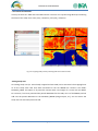
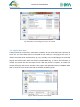
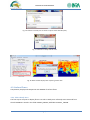
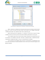
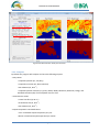
EVASPA.v01 USER MANUAL EVASPA.v01 USER MANUAL
Contributing Authors: Gallego‐Elvira B., Olioso A., Mira M., Castillo S., Lecerf R., Weiss M., Courault D. EVASPA.v01 USER MANUAL CONTENTS
1. INTRODUCTION ................................................................................................................................................... 2 2. INSTALLATION ..................................................................................................................................................... 2 3. INPUT DATA ......................................................................................................................................................... 3 3.1. Images .......................................................................................................................................................... 3 3.1.1. MODIS .................................................................................................................................................. 3 3.1.2. OTHER ................................................................................................................................................... 4 3.2. Meteorological data .................................................................................................................................... 4 3.3. Digital Elevation Model (DEM) ..................................................................................................................... 4 4. MENU DESCRIPTION ........................................................................................................................................... 5 4.1. Import Images .............................................................................................................................................. 5 4.2. New Study Area ........................................................................................................................................... 8 4.2.1. Select Imported Database .................................................................................................................... 8 4.2.2. Extraction ........................................................................................................................................... 10 4.2.3. Import Meteo Data ............................................................................................................................. 13 4.3. Surface Fluxes ............................................................................................................................................ 14 4.3.1. Select Study Area ................................................................................................................................ 14 4.3.2. Compute ............................................................................................................................................. 16 4.3.3. View .................................................................................................................................................... 17 4.3.4. Compare with MOD16 ........................................................................................................................ 24 5. THEORETICAL BACKGROUND ............................................................................................................................ 26 5.1. ET mapping algorithm ................................................................................................................................ 26 5.2. Calculation of LE and ET ............................................................................................................................. 28 5.3. Calculation of Rn ......................................................................................................................................... 28 5.4. Equations for G computation .................................................................................................................... 29 5.5. Determination on EF .................................................................................................................................. 29 5.6. Interpolation of daily ET ............................................................................................................................ 30 5.7. Selection of Study Areas ............................................................................................................................ 30 6. PROCESSING OF INPUT VARIABLES ................................................................................................................... 30 6.1. Surface Temperature and Emissivity ......................................................................................................... 30 6.2. NDVI and Fc ............................................................................................................................................... 31 6.3. Albedo ........................................................................................................................................................ 31 6.4. LAI .............................................................................................................................................................. 31 6.5. Water mask ................................................................................................................................................ 31 6.6. Slope mask ................................................................................................................................................. 31 REFERENCES .......................................................................................................................................................... 32 Page | 1 EVASPA.v01 USER MANUAL 1.INTRODUCTION
EVASPA is a tool to compute surface energy fluxes from remotely sensed images. The following variables can be estimated: ‐ Evapotranspiration (ET) ‐ Net Radiation (Rn) ‐ Evaporative fraction (EF) ‐ Ground heat flux (G) The flux computation algorithms of EVASPA.v01 are based on the S‐SEBI method (Roerink et al. 2000) and the triangle approach (Carlson 2007). Both methods assume that over large areas, those areas with very high (or low) evaporation can be identified from contextual remotely sensed information. Algorithms based on aerodynamic approaches will be included in next versions and the variable sensible heat flux (H) will be provided. This tool is being developed within the frame of SIRRIMED (Sustainable use of IRRgation water in the MEDiterranean Region, FP7, European Commission) and TOSCA (Earth, Ocean, Continental Surfaces and Atmosphere, Centre National d’Etudes Spatiales (CNES, France)). 2.INSTALLATION
EVASPA.v01 is a software developed using MATLAB© language and can be installed on any computer working under windows OS system. It is a compiled version that does not require to install MATLAB© on the computer. To use EVASPA.v01, the Matlab Component Runtime (MCR) needs to be installed. MCR is a collection of libraries required to run compiled MATLAB© codes. It essentially includes all the existing MATLAB© libraries, but does not require a license to be installed. Installing the MCR assures that the code behaves exactly like it would under MATLAB©. To install EVASPA.v01: 1. Create a new folder where you would like to install EVASPA. 2. Copy the file: EVASPA_v01x86_pkg (32 bits) or EVASPA_v01x64_pkg (64 bits), depending on Windows version, to the previously created folder. 3. Execute the file that you have just copied and follow the instructions. EVASPA and the Matlab compiler runtime will be installed. 4. To run EVASPA.v01 click on EVASPA_v01.exe. Page | 2 EVASPA.v01 USER MANUAL 3.INPUTDATA
To compute surface fluxes with EVASPA, the input remotely sensed images, DEM (Digital Elevation Model) and meteorological data must meet the format requirements described in the following sections. 3.1.Images
3.1.1.MODIS
EVASPA.v01 processes MODIS TERRA and AQUA images in EOS‐HDF format. Table 1 shows the MODIS products required. Shortname
Platform
MODIS Product
Raster
Res
Temporal
type
(m)
Granularity
*MOD15A2
Terra
Leaf Area Index - FPAR
Tile
1000m
8 day
MCD15A3
Combined
Leaf Area Index - FPAR
Tile
1000m
4 day
MOD44W
Terra
Land Water Mask Derived
Tile
250m
None
**MYD11A1
Aqua
Tile
1000m
Daily
MCD43B1
Combined
BRDF-Albedo Model Parameters
Tile
1000m
16 day
MCD43B3
Combined
Albedo
Tile
1000m
16 day
MYD13A2
Aqua
Vegetation Indices
Tile
1000m
16 day
MOD13A2
Terra
Vegetation Indices
Tile
1000m
16 day
MCD43B2
Combined
BRDF-Albedo Quality
Tile
1000m
16 day
MOD11A1
Terra
Tile
1000m
Daily
Land Surface Temperature &
Emissivity
Land Surface Temperature &
Emissivity
Table 1. MODIS products required by EVASPA.V0.1. Source: https://lpdaac.usgs.gov/products/modis_products_table *MOD15A2: Only required for the period: 18/02/2000‐03/07/2002, since MCD15A3 was not yet available. Note that for that period the input LAI images temporal scale is 8day. **MYD11A1: Optional product, the program can be run without this input. For further information about the products, the user is referred to: https://lpdaac.usgs.gov/products/modis_products_table All these products can be downloaded, free of charge, from the Web page of NASA REVERB http://reverb.echo.nasa.gov/reverb/. The required version of the products is 005. Page | 3 EVASPA.v01 USER MANUAL Apart from these products, which are required to compute the surface fluxes, EVASPA.v01 offers the possibility to compare the results on Evapotranspiration mapping against the MOD16 global evapotranspiration product provided by the “Numerical Terra dynamic Simulation Group” (NTSG) of the University of Montana. All information about this product can be found in: http://www.ntsg.umt.edu/project/mod16 EVASPA.v01 processes MOD16 on monthly and yearly scale. The images can be downloaded from the previous link (Data Product Tab) in HDF format on monthly and yearly scale or from the ftp server: ftp.ntsg.umt.edu (User: anonymous, Password: email address, ex: [email protected]). 3.1.2.OTHER
EVASPA.v01 only processes MODIS images. The next version, EVASPA.v02, will include the option to process Landsat images. Images from other sensors will be incorporated in next versions. 3.2.Meteorologicaldata
The ground data variables needed for computation are: ‐
Incoming solar radiation (Rs, W m‐2) ‐
Incoming long‐wave (atmospheric) radiation (Ra, W m‐2) The meteorological data should be available at time scale lower than daily. 10min, 30min or hourly time scale are recommended, since the software will select for calculations the closest recording time of meteo data to satellite overpass time. The format required is CSV (separation semicolon). MS Excel files can be saved in this format. The meteo file must have 3 columns: (i) First: Date and time in format: dd/mm/yyyy HH:MM, (ii) Second: Rs (W m‐2) and (iii) Third: Ra (W m‐2). The fill value, for example ‐9999, will have to be indicated (see section 4.2.3). During night time, Rs should be set to zero, negative or fill values during these hours must be replaced by zeros. An example of meteo file (EVASPAV01_MeteoFileTemplate.csv) is provided with this manual. 3.3.DigitalElevationModel(DEM)
A DEM is required in this EVASPA version to mask areas above a certain altitude. In the next version it will be required to generate a slope mask. The computations can be run without DEM. For information regarding the Slope Mask, see section 6.6. For MODIS images the global digital elevation model (DEM) GTOPO30, provided by U.S. Geological Survey's EROS Data Center (EDC) can be downloaded, free of charge, from: http://www1.gsi.go.jp/geowww/globalmap‐gsi/gtopo30/gtopo30.html Page | 4 EVASPA.v01 USER MANUAL The format required by EVASPA is a text file, named: gtopo_ h##v##. The DEM GTOPO30 for the tile h18v04 is provided as an example with this manual. The dimensions of the DEM matrix in the text file have to be 1200 rows and 1200 columns, like MODIS tiles (pixel size: 926.62 m, sinusoidal projection). 4.MENUDESCRIPTION
4.1.ImportImages
Raw images are imported and stored to be used in calculations. MODIS When we click on Import Images: MODIS, a window (Fig.1) will open to ask to for the “Raw Data folder”. The user has to indicate the folder in which the HDF files of MODIS products are stored. This folder must contain one subfolder for each product. The subfolder must be named like the shortname of the products. Fig.1 shows the structure and subfolder names for the “Raw Data folder”. Raw Data Folder to be selected Optional Subfolders Only for : 18/02/2000‐03/07/2002 Optional Fig. 1. Example of Raw Data Folder. Page | 5 EVASPA.v01 USER MANUAL As above‐mentioned, the products MYD11A1 and MOD16 and the DEM are not compulsory required for calculations, but they provide valuable additional information. Note that the subfolder “MOD16” has two subfolders to store Monthly and Yearly images. The original name of the raw images downloaded from REVERB or NTSG must not be altered. The HDF file name has the following format: ESDT.AYYYYDDD.hHHvVV.CCC.YYYYDDDHHMMSS.hdf ESDT = Earth Science Data Type name (e.g., MOD14A1) YYYYDDD = MODIS acquisition year and DOY HH = Horizontal tile number (0‐35) VV = Vertical tile number (0‐17) CCC = Collection version number (001, 002, 003, etc.) (NOTE: 005 for EVASPA.v01) YYYYDDDHHMMSS = Processing Year, Julian day and UTC Time hdf = Suffix denoting HDF file Examples: ‐ MCD15A3.A2009169.h18v04.005.2009180054227.hdf ‐ MYD13A2.A2009169.h18v04.005.2009200110759.hdf For MOD16 images, YYYYDDD is replaced for monthly scale by YYYYMMM (acquisition year and month) and for yearly scale by YYYYnnn (acquisition year and last day of the year). Examples: ‐ MOD16A2.A2009M06.h18v04.105.2010357212125.hdf (MOD16/Month) ‐ MOD16A3.A2009365.h18v04.105.2010356040241.hdf (MOD16/Year) Once the Raw Data Folder has been selected, a new window (Fig.2) will open to ask for the TILE INFO. The standard MODIS tile nomenclature, h##v##, denotes the horizontal (h) and vertical (v) position of the MODIS tile. Fig. 3 shows an overview of all MODIS tiles. The information about h and v, it is always part of the HDF file name, for example: MOD11A1.A2009170.h18v04.005.2009171184605.hdf Fig. 2. TILE INFO window. Page | 6 EVASPA.v01 USER MANUAL Note: The subfolder of the Raw Data may contain HDF files of different tiles, but only those images corresponding to the selected tile will be processed. EVASPA.v01 will create one database per tile for computations. The import process should be done tile by tile. Fig. 3. MODIS Sinusoidal Tiling System. Source: https://lpdaac.usgs.gov After inserting the values of v and h in the TILE INFO window, another window will open to ask the user where to store the program outputs. EVASPA.v01 will create the folder “EVASPA_MODIS” in which all the information generated by the program will be stored. Fig. 4. Selection of Output directory. Page | 7 EVASPA.v01 USER MANUAL In the selected Output Directory, in the Folder EVASPA_MODIS, the subfolder: DataBase_h##v## will be created to store all imported images corresponding to the tile h##v##. The image importing process can take some time, depending on the number of images and the computer features. Several waitbars, like Fig. 5, will pop up while the images are being imported. When the process is finished, an information window (stating “The DataBase has been created”) will pop up and the information of the “CURRENT DATABASE” will be updated (Fig.6). Fig. 5. Waitbar of data importing process. Fig. 6. End of data importing process. 4.2.NewStudyArea
Each MODIS tile covers an area of ~1100 km x 1100 km (Image Dimensions: 1200 rows x 1200 columns, Spatial Resolution: 0.926 km). Within the tile, several areas of interest (study areas) can be cropped out for calculations. The study area requirements for optimal algorithm performance are described in section 5.7. 4.2.1.SelectImportedDatabase
The first step to create a new study area is to select the imported Database of a certain tile h##v##. Page | 8 EVASPA.v01 USER MANUAL Fig. 7. Selection of imported Data Base to create new study areas. When an imported Database is selected, the main window of the program will display the name and source of images (Ex: MODIS, Landsat etc.) in the “CURRENT DATABASE” info and it will show the overview of the selected tile (Fig. 8). Note: The size of the DataBase_ h##v## folder for a full year is about 10 Go. Fig. 8. Information showed in the main window when a Database is selected. Page | 9 EVASPA.v01 USER MANUAL 4.2.2.Extraction
To extract a study area from the tile, there are 3 options: ‐ Crop from Image When selecting this option, an image of the tile will pop up in which the user can graphically crop a study area (square or rectangular). Once the area is selected, right‐click and click on “crop image” (Fig. 9). Afterwards, the program will ask the user for the ID number of the study area and for comments or key words to remember/identify the area (Fig. 10). Fig. 9. Cropping study area from tile image. Fig. 10. Request of Study Area Information. Page | 10 EVASPA.v01 USER MANUAL Finally, only if a DEM is available in the Database, the program will ask to select the maximum elevation to be considered in the study area. All surfaces above the selected maximum elevation will be masked. The information regarding this mask can be found in section 6.6. Fig. 11. Selection of maximum elevation. After these input dialog windows (Fig. 9 and 10), the extraction of study area will start. Several waitbars will pop up to show the program progress. The program will extract TERRA images and AQUA and/or MOD16 images when available. This process can take some time, depending on the number of images and the computer features. When the process is completed, an information window will pop up and the main window of the program will update the INFO of “CURRENT STUDY AREA” and it will show the overview of the tile, study area, and water and slope mask (Fig. 12). Fig. 12. Main window display after study area extraction. Page | 11 EVASPA.v01 USER MANUAL ‐ Insert Rows and Columns In every tile there are 1200 rows and 1200 columns. The user can crop the image directly introducing the limits of the study area: row1 (min), row2(max), col1 (min), col2(max). Col1 Col2 Row1 Row2 Fig. 13. Cropping study area by inserting rows and columns limits. ‐Exiting Study Area An existing study area (i.e. area already cropped and extracted) can be extracted. The cropping limits of all the study areas that have been extracted for the tile h##v## are stored in the folder: DataBase_h##v#. This option is of particular interest when new images of a certain tile are added. For instance, if we have processed the period 2003‐2007 for the study area i of tile h##v##, and we add now the period 2007‐2011 to the DataBase_h##v## (Image Import, 4.1), we can extract the study area i for the latter period as well. Page | 12 EVASPA.v01 USER MANUAL Fig. 14. Selection of an existing study area to be cropped. 4.2.3.ImportMeteoData
The computation of surface fluxes requires the availability of the meteorological data described in section 3.2. The meteo data need to be extracted for each study area. The program will ask for to indicate the CSV file with the meteo data (Fig. 15), the study area corresponding to the meteo file (Fig. 16) and the fill value of the CSV file, for example ‐9999 (Fig. 17). When that information is inserted, the program will start the import process. When the process is completed, an information window will pop up and the main window of the program will update the INFO of “CURRENT STUDY AREA” to show the name of the meteo file and the data availability (Fig. 18). Fig. 15. Selection of meteo data file (CSV). Page | 13 EVASPA.v01 USER MANUAL Fig. 16. Selection of study area in which to import meteo data file (CSV). Fig. 17. Selection of study data fill value. Fig. 18. Main window display after importing meteo data. 4.3.SurfaceFluxes
Computation, display and comparison with MOD16 of surface fluxes. 4.3.1.SelectStudyArea
The first step to compute or display fluxes is to select a Study Area. All Study Areas extracted from the tile h##v## are stored in the folder EVASPA_MODIS, subfolder DataBase_ h##v##. Page | 14 EVASPA.v01 USER MANUAL Fig. 19. Selection of Study Area for computation or display of surface fluxes. When a study area is selected, the main window will show the overview of the tile and the study area, as well as the water and slope masks and the INFO of the “CURRENT DATA BASE”, “CURRENT STUDY AREA” and “SURFACE FLUXES” will be updated (Fig. 20). Before launching the flux computation, it is important to check that the period of image availability matches up with the period of meteo data availability (Underlined in red in Fig. 20). For the display options, there must be fluxes already computed for the selected study area. In the INFO box, the availability of flux data is indicated in “SURFACE FLUXES”: “COMPUTED FLUXES”. If the INFO box “COMPUTED FLUXES” is empty, no computed fluxes are available. For the comparison with MOD16 images, apart from computed fluxes, the MOD16 data need to have been extracted for the selected study area. If that is the case, this info will also appear in the INFO box “MOD16”. Page | 15 EVASPA.v01 USER MANUAL Fig. 20. Main Window after Study Area selection. 4.3.2.Compute
By default the program will compute and save the following outputs: ‐ Daily values: ‐ Evapotranspiration (ET, mm/day) ‐ Evaporative Fraction (EF, dimensionless) ‐ Net radiation (Rn, W m‐2) ‐ Evapotranspiration statistics (ET_Stats): Mean, Mode, Maximum, Minimum, Range, and Standard Deviation (SD) of all computed versions of ET. ‐ Instantaneous values: ‐ Latent heat flux (LE, W m‐2) ‐ Ground heat flux (G, W m‐2) ‐ Net radiation (Rn, W m‐2) ‐ Evapotranspiration cumulated values ‐ Year: Cumulated evapotranspiration per year ‐ Month: Cumulated evapotranspiration per month Page | 16 EVASPA.v01 USER MANUAL Before computing the fluxes, a window will pop up to select the “Saving Options” (Fig. 21). The user can choose which outputs will be saved. The outputs of the flux computation will be stored in: EVASPA_MODIS\ SurfaceFluxes_ h##v##\Satellite_Name\StudyArea_N. Fig. 21. Selection of saving options. After selecting the saving options, the computation will start. Several waitbars will pop up to show the program progress. This process can take some time, depending on the number of images and the computer features. When the process is completed, an information window will indicate that “The fluxes have been computed” and the main window of the program will update the INFO of “SURFACE FLUXES”. 4.3.3.View
Note: For all display options, a study area from the DataBase_ h##v## must be selected. If the INFO box “COMPUTED FLUXES” is empty, no computed fluxes are available to be displayed. ‐ Flux Map Once the study area has been selected, maps of any stored flux can be displayed (Fig. 22, 23). For each flux different versions are available, e.g. there are 42 versions of daily evapotranspiration and 14 versions of ground heat flux. The name of the folder indicates the version. Details on flux version names are provided in section 5. Page | 17 EVASPA.v01 USER MANUAL Fig. 22. Selection of flux map to be displayed. Page | 18 EVASPA.v01 USER MANUAL Fig. 23. Display of flux map. ‐ Point Profile This option shows the evolution of daily and monthly evapotranspiration throughout one year in a certain location (pixel). The graphs displayed show: the evolution of daily evapotranspiration for all versions (including mean and SD), the evolution of evapotranspiration on daily and monthly scale for a selected version, and the boxplot (box‐and‐whisker diagram) of all ET versions on monthly scale (Fig. 27). The pixel (point) to be displayed can be selected by inserting its location in the tile or in the study area. Page | 19 EVASPA.v01 USER MANUAL ‐ Row and Col in Tile The MODLAND Tile Calculator, provides the location within the tile of any point by inserting the geographic coordinates (http://landweb.nascom.nasa.gov/cgi‐bin/developer/tilemap.cgi). For example (Fig. 24), the location of the point latitude: 43.5, longitude: 4.5 is: tile h18v04, line: 779, column (samp): 391. Fig. 24. MODLAND Tile Calculator. Location of the point latitude: 43.5, longitude: 4.5. Page | 20 EVASPA.v01 USER MANUAL ‐ Row and Col in Study Area The user can also insert directly the location within the study area, for example (Fig. 25), Pixel line: 52, Col:80. Line 52 Col 80 Fig. 25. Location of a point within the study area. Page | 21 EVASPA.v01 USER MANUAL Fig. 26. Information required for point profile display. Page | 22 EVASPA.v01 USER MANUAL Fig. 27. Graphs produced in the point profile display option. Page | 23 EVASPA.v01 USER MANUAL 4.3.4.ComparewithMOD16
Evapotranspiration maps and point profiles can be compared against the MOD16 global evapotranspiration product on monthly and yearly scale. For the comparison with MOD16 images, computed fluxes and MOD16 data need to available for the selected study area for the same period (check availability in the info box “SURFACE FLUXES”). ‐ Whole Study Area This option displays the graphs (Fig. 28) of cumulated Monthly or Yearly ET maps of a certain version, the map of MOD16 for the same month/year, the difference ET_EVASPA – ET_MOD16 and the density scatter plot ET_EVASPA vs. ET_MOD16 (includes regression line and coefficient). Fig. 28. Display of map comparison with MOD16. Page | 24 EVASPA.v01 USER MANUAL ‐ Point Profile This option displays the graphs (Fig. 29) of cumulated Monthly ET of the selected version in the selected pixel, the scatter plot ET_EVASPA vs. ET_MOD16 (includes regression line and coefficient) and the boxplot of all ET versions on monthly scale plus MOD16. In the same way as for Point Profile Display (section 4.33), the pixel to be displayed can be selected from line and column in the tile or the study area. Fig. 29. Display of point profile comparison with MOD16. Page | 25 EVASPA.v01 USER MANUAL 5.THEORETICALBACKGROUND
5.1.ETmappingalgorithm
The following figure shows the flow diagram of the algorithm for mapping ET from MODIS. Fig. 30. Algorithm for mapping ET from MODIS data. Algorithms of EVASPA are based on the S‐SEBI method (Roerink et al. 2000) and the triangle approach (Carlson 2007). S‐SEBI is a simplified method derived from SEBI which consists of determining a reflectance dependent maximum (respectively minimum) temperature for dry (respectively wet) conditions (Fig. 31). Carlson (2007) gives a good overview of the triangle method for estimating ET. The method is based on the physically meaningful relationship between the evaporative fraction and the combination of the remotely sensed surface temperature (Ts) and NDVI (Normalized Difference Vegetation Index,) or Fc (Fraction Cover). The scatter plot Ts vs. NDVI (or Fc) has a triangle shape whose boundaries are interpreted as limiting surface fluxes, the upper limit being the dry edge and the lower limit being the wet edge (Fig. 32). Page | 26 EVASPA.v01 USER MANUAL Fig. 31. Theoretically schematic relationship between surface temperature and albedo in the S‐SEBI model. Source: (Li et al. 2009) Fig. 32. Summary of the key descriptors and physical interpretations of the surface temperature / vegetation index “triangular” space or ‘scatterplot’. Source: (Petropoulos et al. 2009) Page | 27 EVASPA.v01 USER MANUAL The mapping algorithm is designed to include several methods for deriving the basic inputs used to compute ET, such as evaporative fraction EF, G, Rn. In this way, several estimates of ET can be provided depending on the assumptions made on the reliability of the inputs. This provides, in a way, an assessment of the level of uncertainties in the derivation of ET. The name of the folders in which outputs are stored indicate which equations have been used. For example: G_4_rn_1_em_2: Equation 4 is used to compute G (section 5.4) and Equation 2 is used to compute emissivity (section 6.1). The folders that contain EF, LE and ET will include in the name: “alb_1_ndvi_0_fc_0” or “alb_0_ndvi_1_fc_0” or “alb_0_ndvi_0_fc_1”. The “1” indicates that that variable is used, for example, alb_0_ndvi_0_fc_1 means that Fc has been used in computations. 5.2.CalculationofLEandET
The latent heat flux, LE, is normally computed from instantaneous values of EF, Rn and G: LE_1= EF (Rn ‐ G) (1) For cases in which net long‐wave radiation is not available, LE may be computed from EF, Rs and G: LE_2= EF (Rs ‐ G) (2) Both options, LE_1 and LE_2, are computed to assess the differences between them. The daily ET is computed from EF (assumed to be constant during the day) and the daily net radiation (Rn,d), which is estimated from instantaneous net radiation (Rn,i). ET_1=EF* Rn,d (3) 5.3.CalculationofRn
The instantaneous net radiation, Rn,i, it is calculated with the following expression: Rn_1= ,
1
(4) Rs= Solar radiation (ground data) Ra= Incoming long‐wave radiation (ground data) α = Albedo Ts= Surface temperature ε= Emissivity To derive the daily net radiation (used in Eq. 3) from the instataneous values (Rn,d = Rn,i *C), the ratio between daily net radiation and instantaneous net radiation (C= Rn,d / Rn,i) versus the day of the year (DOY) is used. The equations were obtained from net radiation fluxes measured at the Page | 28 EVASPA.v01 USER MANUAL meteorological station of the “El Saler” area, located in the East coast of the Iberian Peninsula (Valencia, 39° 20′ 41.165″ N, 0° 19′ 12.031″ W, at sea level) (Sobrino et al. 2007). NOTE: This relathionship (C) needs to be adapted for the different locations in which EVASPA is applied. Since the equation derived for “El Saler” is used instead a locally‐derived one, it is therefore a source of inaccuracy in EVASPA.v01. EVASPA.v02 will include the option to derive C for each study area. 5.4.EquationsforGcomputation
The ground heat flux is computed from Rn,i and depending on the version, some of the following variables,: Ts, albedo, NDVI, Fc, LAI, EF. Seven equations are considered for the calculation. The sources of the equations are: G1: G=0; G2: (Bastiaanssen et al. 1998) G3: (Su 2002) G4: (Kustas et al. 1993) G5: (Choudhury et al. 1987) G6: (Moran et al. 1994) G7: (Tanguy et al. 2012) 5.5.DeterminationonEF
Seven versions are considered for the determination of wet and dry edges of the triangle space (Ts‐
NDVI, Ts‐Fc) or the radiation and evaporation control limits of the space Ts‐Albedo: EF1: Simplified version of the algorithm proposed by (Tang et al. 2010), without outlier filtering. EF2: Full version of Tang et al. 2010. EF3: The edges are horizontal lines equal to the maximun and minimun surface temperature observed in the image. EF4: Algorithm provided by J. A. Sobrino of the Unit Global Change, University of Valencia (Sobrino et al. 2005). EF5: The wet/evaporation control edged is set to the minimun surface temperature observed in the image (horizontal line) and the dry/radiation control edge is a 3rd degree polynomial. EF6: Same as EF5 but with a filter of outliers. EF7: Tang et al. 2010 with a prefiltering of outliers. Page | 29 EVASPA.v01 USER MANUAL 5.6.InterpolationofdailyET
For days with no data acquisition or presence of clouds, ET is interpolated. ET is reconstructed from a linear interpolation of the ratio ET/Rs between the discrete satellite ET estimates available for clear days (Delogu et al. 2012, Lagouarde et. 2010). One of the main targets for next EVASPA version is to improve the ET interpolation, since the main application of the tool is to provide continuous information on daily ET. 5.7.SelectionofStudyAreas
The assumptions made by the ET algorithms implemented in EVASPA.v01 require large and heterogeneous study areas, since the spatial variability is used to determine “dry” surfaces and “wet” surfaces. In the triangle method, the interpretation of the Ts−NDVI or Ts−Fc space implies that within each vegetation type the observed surface temperature ranges from a minimum with the strongest evaporative cooling to a maximum with the weakest evaporative cooling. This means that the observed dry edge of the triangular space represents the lowest evaporative fractions for varying NDVI or Fc and the wet edge represents maximum evaporative fractions. The approach is valid when both minimum and maximum evapotranspiration can be observed within the boundaries of the study area, and an important assumption is that these different cases are not primarily caused by differences in atmospheric conditions but by variations in water availability (Stisen et al. 2008). Similarly, for the S‐SEBI method (Roerink et al. 2000), in which a reflectance dependent maximum (respectively minimum) temperature for dry (respectively wet) conditions are determined, contrasted surface reflectances (albedo) have to be present on the study area. 6.PROCESSINGOFINPUTVARIABLES
The input variables Ts, Emissivity, NDVI, and albedo are provided by MODIS products. The quality bands of the products are used to filter low quality input data. 6.1.SurfaceTemperatureandEmissivity
The MODIS product MOD11A1 provides daily Land Surface Temperature and Emissivity (Band 31 and Band 32). Only a scale factor is needed to get the Ts values. Two equations are used to calculate emissivity, that combine the Band 31 and Band 32 emissivity. EM1: (Jin and Liang 2006) EM2: (Tang et al. 2010) Page | 30 EVASPA.v01 USER MANUAL 6.2.NDVIandFc
MYD13A2 (AQUA) and MOD13A2 (TERRA) provide NDVI data. Global MYD13A2 data or MOD13A2 are provided every 16 days at 1‐kilometer spatial resolution. The production is phased between TERRA and AQUA acquisitions, with Terra beginning on Day 001 and Aqua beginning on Day 008. Phased production for improved temporal frequency is considered in EVASPA (8‐days temporal resolution combining TERRA and AQUA products). The fraction cover is derived from NDVI values using the formula proposed by (Carlson and Ripley 1997). 6.3.Albedo
The products MCD43B1, MCD43B2 and MCD43B3 provide the information to calculate albedo and assess the quality of the data. 6.4.LAI
LAI is provided by level‐4 combined (TERRA and AQUA) MCD15A3 product, composited every 4 days at 1‐kilometer resolution. This product is available since 03/07/2002. For earlier dates (only TERRA images), MOD15A2 is used is instead, which provides 8‐day LAI data. 6.5.Watermask
When using the S‐SEBI and triangle methods, the open‐water surfaces are commonly masked. The land water mask provided by MODIS, MOD44W, is used to filter water surfaces before computing Evaporative Fraction. The water bodies evaporation can be estimated with aerodynamic equations from the water surface temperature (McJannet et al. 2012). EVASPA.v02 will prodides open‐water evaporation estimates. 6.6.Slopemask
There are topographic effects on MODIS LST in complicated terrains. High‐resolution DEM is an important input to make pixel‐specific topographic correction for localized radiometric effects (slope/aspect related illumination differences, shadowing, and reflection of radiation from adjacent pixels). Only the first order of topographic information, i.e., the elevation of the surface, is considered in radiative transfer simulations in the development of MODIS LST algorithms. In rugged areas where high resolution DEM is not available, it is difficult to accurately estimate land surface temperature (Wan 1999). The LST is one of the main inputs for ET mapping in EVASPA, and important under/overestimations can be produced if this aspect is not taken into account. Work is in progress to implement an efficient slope masking (based on a DEM) that prevents the ET maaping errors Page | 31 EVASPA.v01 USER MANUAL derived from these effects. At the moment, only a masking based on elevation has been implemented to mask mountainous areas in which this problem can appear. When a DEM is available, the user has the option to mask all areas above a certain altitude. REFERENCES
Bastiaanssen WGM, Menenti M, Feddes RA, Holtslag AAM (1998) A remote sensing surface energy balance algorithm for land (SEBAL) ‐ 1. Formulation. Journal of Hydrology 213 (1‐4):198‐212 Carlson T (2007) An overview of the "triangle method" for estimating surface evapotranspiration and soil moisture from satellite imagery. Sensors 7 (8):1612‐1629. doi:10.3390/s7081612 Carlson TN, Ripley DA (1997) On the relation between NDVI, fractional vegetation cover, and leaf area index. Remote Sensing of Environment 62 (3):241‐252. doi:10.1016/s0034‐4257(97)00104‐1 Choudhury BJ, Idso SB, Reginato RJ (1987) Analysis of an empirical‐model for soil heat‐flux under a growing wheat crop for estimating evaporation by an infrared‐temperature based energy‐balance equation. Agricultural and Forest Meteorology 39 (4):283‐297. doi:10.1016/0168‐1923(87)90021‐9 Delogu E, Boulet G, Olioso A, Coudert B, Chirouze J, Ceschia E, Le Dantec V, Marloie O, Chehbouni G, and Lagouarde J‐P (2012) Reconstruction of temporal variations of evapotranspiration using instantaneous estimates at the time of satellite overpass, Hydrol. Earth Syst. Sci. 16: 2995‐3010, doi:10.5194/hess‐16‐2995‐2012, 2012. Jin M, Liang S (2006) An improved land surface emissivity parameter for land surface models using global remote sensing observations. Journal of Climate 19 (12):2867‐2881. doi:10.1175/jcli3720.1 Kustas WP, Daughtry CST, Vanoevelen PJ (1993) Analytical treatment of the relationships between soil heat‐flux net‐radiation ratio and vegetation indexes. Remote Sensing of Environment 46 (3):319‐
330. doi:10.1016/0034‐4257(93)90052‐y Lagouarde J.‐P., Olioso A., Boulet G., Coudert B., Dayau S., Castillo S., Weiss M., Roujean J.‐L., Delogu E. et Puche N., 2010. Defining the revisit frequency for the MISTIGRI project of a satellite mission in the thermal infrared. Third Recent Advances in Quantitative Remote Sensing (RAQRS), Torrent er (Valencia, Spain), 27 septembre – 1 octobre 2010. J.A. Sobrino (ed.). Universitat de València, Spain. ISBN: 978‐84‐370‐7952‐3. Pages: 824‐829 Li Z‐L, Tang R, Wan Z, Bi Y, Zhou C, Tang B, Yan G, Zhang X (2009) A Review of Current Methodologies for Regional Evapotranspiration Estimation from Remotely Sensed Data. Sensors 9 (5):3801‐3853. doi:10.3390/s90503801 McJannet DL, Webster IT, Cook FJ (2012) An area‐dependent wind function for estimating open water evaporation using land‐based meteorological data. Environmental Modelling & Software 31:76‐83. doi:10.1016/j.envsoft.2011.11.017 Moran MS, Clarke TR, Inoue Y, Vidal A (1994) Estimating crop water‐deficit using the relation between surface‐air temperature and spectral vegetation index. Remote Sensing of Environment 49 (3):246‐263. doi:10.1016/0034‐4257(94)90020‐5 Page | 32 EVASPA.v01 USER MANUAL Petropoulos G, Carlson TN, Wooster MJ, Islam S (2009) A review of T(s)/VI remote sensing based methods for the retrieval of land surface energy fluxes and soil surface moisture. Progress in Physical Geography 33 (2):224‐250. doi:10.1177/0309133309338997 Roerink GJ, Su Z, Menenti M (2000) S‐SEBI: A simple remote sensing algorithm to estimate the surface energy balance. Physics and Chemistry of the Earth Part B‐Hydrology Oceans and Atmosphere 25 (2):147‐157. doi:10.1016/s1464‐1909(99)00128‐8 Sobrino JA, Gomez M, Jimenez‐Munoz C, Olioso A (2007) Application of a simple algorithm to estimate daily evapotranspiration from NOAA‐AVHRR images for the Iberian Peninsula. Remote Sensing of Environment 110 (2):139‐148. doi:10.1016/j.rse.2007.02.017 Sobrino JA, Gomez M, Jimenez‐Munoz JC, Olioso A, Chehbouni G (2005) A simple algorithm to estimate evapotranspiration from DAIS data: Application to the DAISEX campaigns. Journal of Hydrology 315 (1‐4):117‐125. doi:10.1016/j.jhydrol.2005.03.027 Stisen S, Sandholt I, Norgaard A, Fensholt R, Jensen KH (2008) Combining the triangle method with thermal inertia to estimate regional evapotranspiration ‐ Applied to MSG‐SEVIRI data in the Senegal River basin. Remote Sensing of Environment 112 (3):1242‐1255. doi:10.1016/j.rse.2007.08.013 Su Z (2002) The Surface Energy Balance System (SEBS) for estimation of turbulent heat fluxes. Hydrology and Earth System Sciences 6 (1):85‐99 Tang R, Li Z‐L, Tang B (2010) An application of the T‐s‐VI triangle method with enhanced edges determination for evapotranspiration estimation from MODIS data in and and semi‐arid regions: Implementation and validation. Remote Sensing of Environment 114 (3):540‐551. doi:10.1016/j.rse.2009.10.012 Tanguy M, Baille A, Gonzalez‐Real MM, Lloyd C, Cappelaere B, Kergoat L, Cohard JM (2012) A new parameterisation scheme of ground heat flux for land surface flux retrieval from remote sensing information. Journal of Hydrology (Amsterdam) 454/455:113‐122. doi:10.1016/j.jhydrol.2012.06.002 Wan Z (1999) MODIS Land‐Surface Temperature Algorithm Theoretical Basis Document (LST ATBD) http://modis.gsfc.nasa.gov/data/atbd/atbd_mod11.pdf Page | 33