1
TCAD Driven CAD
A Journal for Process and Device Engineers
Two-Dimensional ATLAS Device Simulation of Pentacene
Organic Thin-film Transistors
1. Introduction
Source(Au)
Recent years has seen rapid acceleration in the research
and development of organic thin film transistors (OTFTs)
as key components for active matrix displays, radio
frequency identification tags, and many other small scale
integrated circuits. There are many advantages to OTFTs,
such as the flexibility of the plastic fabrication substrate
and the potential cost savings to manufacturers that
adopt a solution process and/or ink-jet printing process.
One of the most widely studied organic semiconductor
materials used for OTFTs is Pentacene. Pentacene-based
OTFTs have a typical field effect mobility of around
1 [cm2/(V sec)]. This is of comparable value to hydrogenated
amorphous silicon. OTFTs on lightweight flexible substrates are expected to eventually replace hydrogenated
amorphous silicon TFT applications on glass substrates.
As need to understand basic device operation, to optimize
device structures, and to consider novel device structures
grows, the importance of numerical device simulation
is rising as well.
2. The Device Structure and Models
In order to simulate I-V characteristics of OTFTs, it is
important to consider how carrier transport in organic
semiconductors is described. In many cases, the space-charge
limited current (SCLC) model is successful in explaining
the conduction current of organic semiconductors. This
is especially true in devices such as organic light-emitting
diodes (OLEDs) and OTFTs. Fortunately, the SCLC
model is suited for use in conjunction with more
conventional carrier drift and diffusion type device
simulators like ATLAS.
In the SCLC model, the carriers are self-trapped. In
addition, one of the most determinant factors for carrier
transport characteristics are the energy distributions of
density of states (DOS) within the bandgap. The TFT module
in ATLAS is able to define these density of state distributions.
Drain(Au)
Pentacene
Si02
Heavily doped Si
Gate
Figure 1. A cross-section of a pentacene organic thinfilm transistor.
The device structure is shown in Figure 1. A staggered
inverted structure is adopted. The thickness of the
oxide layer is 400 [nm] and the Pentacene active layer is
50[nm]. The channel length and width are 20 [um] and
220 [um], respectively. The extracted field-effect mobility is 0.62 [cm2/(Vsec)].
For the purpose of numerical simulation, the energy
band gap of Pentacene is defined 2.8 [eV] from an optical bandgap data of Pentacene [2]. Figure 2 shows energy distribution of DOSs assumed. The acceptor tail
DOS is important and is expressed by an exponential
function of energy.
Continued on page 2....
INSIDE
Exact2: Interconnect Parasitic Capacitance
Simulator from Silvaco . . . . . . . . . . . . . . . . . . . . . . . 3
Laser Simulation Encompassing Molar Fraction
Variation via DevEdit . . . . . . . . . . . . . . . . . . . . . . . . . 7
The Importance of Mesh Definition in
Strained-Si Heterostructure Simulation . . . . . . . . . . . 11
Calendar of Events . . . . . . . . . . . . . . . . . . . . . . . . . . . . 13
In this article, a Pentacene TFT reported by Lin, et al. [1]
is simulated with ATLAS and then compared to their
experimental ID-VD curves.
Volume 12, Number 2, February 2003
Hints, Tips, and Solutions . . . . . . . . . . . . . . . . . . . . . . . . 14
SILVACO
INTERNATIONAL
Figure 3. Simulated (green) ID-VD curves using a constant
mobility model and the experimental (red) curve.
Figure 2. Energy distribution and DOS used within the
ATLAS simulations.
Figure 5 shows a hole concentration distribution and
current flow lines at VD=-100V and VG=-40V. This
illustrates basic device operation and the evaluation of
physical quantities in the device.
3. Simulation Results and Discussion
Figure 3 shows the simulation results (green lines) compared with the experimental data (red lines). The gate
bias-dependent saturation drain currents appear to
agree with the experiment, but the currents in transition
regions, from linear to saturate, are still different.
4. Conclusion
The experimental ID-VD curve of a Pentacene OTFT is
numerically well simulated by ATLAS using the SCLC
model and a field-dependent mobility model. These
numerical simulations are helpful in understanding
OTFT’s basic device operation, an accurate physical
quantity evaluation, and the optimization of device
structures.
Though a constant mobility model is used in the case
illustrated in Figure 3, most organic semiconductor
materials have electric field-dependent carrier drift
mobility. An often-used mobility model has the square
root dependence of a Pool-Frenkel electric field. Such
mobility is expressed as the following:.
E
β
µ = µ0 exp − 0 exp E − γ
T
k BT
References
[1] Y.Lin, D.J.Gundlach, S.F.Nelson, and T.N.Jackson, IEEE ED.,
Vol.44, No.8, 1325(1997).
Where β and γ are fitting parameters. User defined
mobility models are easily consolidated into ATLAS by
means of the ATLAS C-Interpreter option module.
Figure 4 shows the results of using this mobility model.
The results agree with the experimental data.
[2] I,Kymissis, C.D.Dimitrakopoulos, and S.Purushothaman, IEEE
ED., Vol.48, No,6, 1060(2001).
Figure 4. Simulated ID-VD (green) curves using field dependent
mobility model and the experimental (red) curves.
Figure 5. Hole concentration distribution and current flow
lines in the OTFT device.
The Simulation Standard
Page 2
February 2003
Exact2: Interconnect Parasitic Capacitance
Simulator from Silvaco
Introduction
Exact2 from Silvaco is a sophisticated, physically-based
simulation tool for calculating semiconductor interconnect capacitance values. Its purpose is to build a capacitance coefficient database that is usable by any layout
parasitic capacitance (LPE) tool.
In order to accurately calculate these coefficients, it is
important that the actual interconnect structures are
accurately defined. Exact2 achieves this by means of an
internal, physically-based 3D process simulator.
Included with the process simulator is an internal 3D
field solver that calculates the capacitance for each
device layer and structure combination. Exact2 also creates capacitance rule files readable by any LPE tool
through the use of analysis script files, written in LISA
code which is, Silvaco’s dynamic scripting language.
This article presents an overview of Exact2’s features,
capabilities, and use.
Figure 1. Main Exact2 Window.
Overview of Selected Features
and Improvements
Exact2’s processing options are geometric etches and
depositions, or realistic etching and deposition. An
integral optical solver takes photolithography effects
into account. All the relevant properties of realistic
etching, deposition, and optolithographic models are
defined by the user, including the isotropic degree of an
etch or deposition, the critical intensity at which the
photoresist will develop, and finally the wavelength,
aperture, and shape of the exposure source. Exact2
simplifies worst case modeling and data analysis by
applying powerful statistical analysis to geometry
dependent parasitics.
Exact2’s 3D process simulation engine simulates many
varieties of arbitrarily complex interconnects, including:
• multiple dielectrics including low-k materials
• multiple metal materials
• non-planar dielectrics
• damascene processing
• conformal deposition
• lithographic effects
Figure 2b. Preview of the process definition created by
the process window.
Figure 2a. The Process window allows each layer of a
process to be defined.
February 2003
Page 3
The Simulation Standard
Figure 3b. When a layout file is loaded this preview window shows the shape of the layer and the variables that
allow its dimensions to be changed.
The Seven Stages of An
Exact2 Experiment
Figure 1 is the main start-up screen of Exact2’s
Graphical User Interface (GUI). There are generally
seven distinct stages that comprise a complete Exact2
experiment, and these stages are identified in Figure 1
by the corresponding icons running down the left hand
side of the main screen.
Figure 3a. The Layout window allows layout files to be
added and defines the combination of layers to be
included in the simulation.
A new paramaterized layout editor and support for the
Language for Interfacing Silvaco Applications (LISA)
enhances custom layouts and analysis capabilities. LISA
also enhances Exact2’s open interface by outputting
data to formats recognized by any chip-level LPE tool.
In addition, custom equations are easy fit to raw parasitic data.
The stages are briefly described as:
1. Process definition: define layer thickness and film
properties
2. Layout definition: choose test structures, layouts,
and layer combinations for each layout
3. Field Solver: control internal field solver attributes
Exact2 dramatically improves upon its predecessor in
several ways, including:
4. Output: specify the result parameters and save location
5. Design of Experiments (DOE): describe the upcoming
experiments
• Extensive use of tool tips throughout the application
• Detailed output logs simplify easier development of
models
6. Run: perform the calculations and generate the database
7. Analysis: analyze, manipulate, and visualize the
generated database
• Results are now saved in plain text for easier retrieval
• Greater control over the simulation domain
Exact2 features two modes of operation (Figure 1):
standard and advanced. The following descriptions are
based on the standard mode of operation.
• Simpler, more robust GUI
• Intuitive approach to results analysis
• Plain text configuration files make it easy to run
Exact2 without the GUI
Figure 4. The field solver used by Exact2 can have different
accuracy levels that control the final capacitance extracted.
The Simulation Standard
Figure 5. The output window allows the user to specify the
database path and output data to be saved.
Page 4
February 2003
Figure 7a.When the experiments are ready to be executed
this Run window shows the status of the submitted jobs.
Figure 6. The design of experiment GUI is used to control
the variation of any layout and/or process variable.
Stage 1: Process definition
User-specific process are easily created with the process
GUI (Figure 2a). This screen is used to input layer definition and thickness, material properties, and parameter variables. Subjects are brought to the foreground by
clicking on the relevant folder heading (Figure 2a). The
user may preview and modify the created process stack
at any time by simply clicking on the preview button in
the process GUI. Figure 2b shows a preview of the
process defined in Figure 2a.
Figure 7b. Simulation monitor window as it appears during
the simulations.
Stage 2: Test structure (layout) definition
Once device layers are identified, the test structures’
mask layout designs are quickly chosen and added to
the experiment with the layout GUI (Figure 3a). Test
structures are easily parameterized and defined in any
combination of selected layers. For example, combination 1 is chosen (left side of Figure 3a) that corresponds
to process layers (right side of Figure 3a). Users can
preview the test structure in both plan and side views
(Figure 3b), and cut lines through any part of the structure are easily implemented.
Stage 3: Field solver
Figure 4 shows the field solver GUI. This screen is used
to adjust of some of the field solver attributes, such as
tolerance and accuracy levels. The probes function
specifically chooses of which pairs of wires will serve as
targets of capacitance calculation. The probes function
is brought to the foreground by clicking on the respective folder heading.
Stage 4: Output
Figure 5 shows the output GUI that is used to specify
the calculation targets and output directories.
Stage 5: Design of experiments (DOE)
This GUI (Figure 6) define the experiment using predefined variables from the process and layout stages. The
only required values are the initial value, final value,
number of data points, and the variation form.
Figure 8. The Run time output window shows the output
from the 3D process simulator and the field solver
capacitance extraction for the current job.
February 2003
Page 5
The Simulation Standard
Figure 9. Exact2 output file structure.
Figure 10. Analysis window used to load and run scripts to
export data files that export the capacitance rule files.
Stage 6: Run
The run stage performs all user-specified calculations
and reports the status and progress back to the user.
Figure 7a shows the screen before calculations are performed, while Figure 7b shows the status further on into
the simulation. Clicking the View log… button (Figure
8) launches the simulation run time output dialog box,
which is useful for reference and error checking. Exact2
outputs a file structure and files that contain each
layer’s simulation results, as well as their respective
combinations and sessions (Figure 9). Users must check
out result files before viewing or modifying them..
Conclusion.
Exact2 brings flexibility and simplicity to the creation
of a comprehensive and accurate interconnect capacitance database. Exact2 creates the database by means of
a 3D process simulator and 3D internal field solver in
one self-contained package. Exact2 files are easily
imported into LPE tool formats through the use of the
LISA scripting language
Stage 7: Analysis.
After a successful simulation run, the script files need to
analyze, manipulate, and visualize the generated database are loaded with the analysis GUI (Figure 10). A
selected script file appear in a text box to the left of the
Browse… function and is into the Analysis stage by
clicking Add. The Run button executes any highlighted
file. The Edit... button launches the built-in text editor
for quick modification to the script file(s).
A simple script file that outputs capacitance data in both
comma separated values (CSV) format and in TonyPlot
format, is shown below. CSV files are easily loaded into
many data management and spreadsheet programs,
such as Microsoft™ Excel™. The resulting TonyPlot file
is shown in Figure 11.
db = DatabaseLoad(".");
extract_name("m0Ctotal_sub", "substrate", "m0_c");
extract_name("m4Ctotal_sub", "substrate", "m4_tmc");
m0_combinations = {1};
m4_combinations = {1};
table_m0 = select(db, "model_0",
m0_combinations,{"m0_subwidth"}, {"m0Ctotal_sub"});
column_scalar_op(table_m0, "m0Ctotal_sub", table_m0,
"m0Ctotal_sub", "*", 1e15);
save_table(table_m0, CSV, "m0_a.csv");
table_m4= select(db, "model_4",
m4_combinations,{"m4_cspace"}, {"m4Ctotal_sub"});
column_scalar_op(table_m4, "m4Ctotal_sub", table_m4,
"m4Ctotal_sub", "*", 1e15);
save_table(table_m4, CSV, "m4_sim_stan.csv");
save_table(table_m4, TONYPLOT, "m4_sim_stan.str");
The Simulation Standard
Figure 11. Simulated total capacitance versus conductor
spacing.
Page 6
February 2003
Laser Simulation Encompassing Molar Fraction
Variation via DevEdit
This article addresses the creation of semiconductor
laser double heterostructures, and the subsequent
simulation of laser output with DevEdit from Silvaco.
A laser consists of a gain medium sandwiched between
two mirrors forming the laser cavity. This is necessary
for effective laser operation because the round trip gain
of the device, including the material and mirror losses,
is unity. In addition, there is an integer number of
half-wavelengths of light inside the optical length of the
laser cavity.
A semiconductor laser consists of a PN junction made
from direct bandgap semiconductor material; the N-doped
side contains excess electrons and there is an excess of
holes on P-doped side. Across this junction is a built-in
potential barrier that prevents or hinders electron-hole
recombination. Forward bias application lowers this
barrier and facilitates carrier recombination. If forward
bias is particularly high, the result is a population
inversion that yields the required gain for laser operation.
Figure 1. The AlGaAs/GaA/AlGaAs stripe laser structure
used in this article.
The interaction between the gain medium and the laser
light is optimized through the use of of double
heterostructures that fabricate a laser from a combination
of semiconductor materials with different band gap
energies. This provides confinement for current and
different refractive indices for optical confinement. The
use of these confinement techniques improves laser efficiencies and lower the laser drive’s current.
The semiconductor materials used for the structure in
this example include GaAs with direct bandgaps of
1.43eV, and AlxGa1-xAs. AlxGa1-x As is dependent on the
x concentration (molar fraction). The x concentration is
the relative number of atoms for which Ga is replaced
by Al. Although x concentration < 0.38 AlxGa1-xAs is a
direct bandgap material, the concentration is higher
and the mertial becomes indirect[1,2]. A variation of the
x concentration is demonstrated here with Silvaco’s
DevEdit device structure editor. Laser simulation of the
device is performed with Laser in conjunction with
Blaze, Silvaco’s 2-D device simulator for III-V, II-VI
materials.
Figure 2. A 1D cutline through the stripe laser shows the xcomposition fraction varying with depth (y) and the donor
and acceptor concentration.
February 2003
Page 7
Figure 1 illustrates the heterostructure stripe laser that
the program is to create. The active layer and photon
generating region is GaAs. Above and below this
region is a cladding layer comprised of Al xGa 1-xAs,
which features a greater bandgap than GaAs. The
resulting discontinuity in the conduction and valence
band edges at the junction of the active layers leads to
confinement of the carrier. The refractive index of the
GaAs region is greater than the Al xGa 1-xAs region,
resulting in an optical confinement in the active layer
that also acts as a slab waveguide. A good quality heterojunction depends on spacing the crystal lattice of the
cladding layer so that it matches the active layer as
closely as possible. This is easily obtained in the
AlGaAs/GaAs structure.
The Simulation Standard
The left column indicates the boundary at which the
doping level, listed in the right column, originates. The
next doping value is found upon reaching the next
boundary (in this example at 0.75 microns). The differing values between the two points require a linear interpolation that results in a linear doping profile. It is possible to define the entire x concentration for the structure
this way. The x concentrations are then added into the
structure only after these doping profiles are written.
The following are important steps for this process:
1. Use ATLAS to create an initial structure without x
concentration.
2. Write a doping profile to use in DevEdit. Save this as
a separate data file.
3. Load the initial ATLAS -designed structure into
DevEdit.
4. Use DevEdit to click on impurities, and then on
doping profile.
Figure 3. At zero bias on the strip laser a 1D cutline can plot the
conduction and valence bands; (a) shows the full depth and (b)
is zoomed in to the GaAs layer,
5. Load the doping profile (the data file written during
stage 2)
6. Click on add impurities.
There are several options that reduce the electrical current
required for the lasing operation. One option makes use
of a stripe contact that effectively limits the lateral extent
of the current injection, and yields a smaller lasing
region of the active material. The injection current flows
through a narrow stripe contact so that even a moderate
injection current yields a high current density within the
active layer. Since gain is achieved only in the high
current density regions, such an arrangement is termed
gain guiding. In the figure, the stripe width of the laser
is 3 microns, the cavity length is 100 microns, while the
x concentration of the AlxGa1-xAs is graded from 0.7 at
the outer edge of the layer to 0.3 at the GaAs junction
7. Choose start x=-2, start y=0, end x=11, end y=0. On a Y
roll off choice, choose the user profile that was created
in step 2.
8. Save the structure with a valid name.
The values chosen for the x fields in Stage 7 are the
beginning and the end value of the x dimension. The
value for the beginning and end of the y field matches
the start value of the y dimension.
Creating the Structure with DevEdit
The initial structure is created with Silvaco ATLAS and
includes the mesh, doping concentrations and electrical
contact. The structure contains no x concentration at this
point. The initial structure is saved for later import into
DevEdit, where the various x concentrations are then
added. The structure is defined by means of a doping
profile written separately the user. It’s important to clearly define x concentrations prior to adding them to the initial structure. Our example profile, illustrated below, is
saved as example_profile.dat.
0
0.7
0.75
0.3
0.85
0.3
2.1
0.7
The Simulation Standard
Figure 4. Simulated photon density versus anode voltage for
the stripe laser.
Page 8
February 2003
Figure 5a. Simulated light intensity of the fundamental
mode of the stripe laser.
Figure 5b. A 1D cutline through the center of the light intensiy at x-5µm.
impact to the charge transport. To align the bandgaps,
use the MATERIAL statement’s ALIGN parameter.
This specifies the fraction of bandgap difference that
appears as conduction band discontinuity. Blaze creates
the desired conduction band and offsets it by modifying
the electron affinity of the material specified in the
ALIGN parameter.
Figure 2(a) illustrates a structure that is divided with a
one dimensional cut line that directly follows the doping
profile and exposes the x concentration. Figure 2(b) presents additional information, such as doping concentration, acceptors and donors, within the structure.
Initial Simulation
The complete structure is obtained from DevEdit and is
then imported into ATLAS for simulation. An important
parameter in a heterostructure device is the bandgap
alignment. The bandgap difference is distributed
between the conduction and valance bands with great
The example assumes a value of ALIGN=0.6 that
results in the assignment of 60% of the bandgap to the
conduction band offset. To save simulation time when
modeling the Fabry-Perot laser, gradually increase the
device bias until the laser threshold voltage is nearly
reached before executing the laser simulation. Only the
electrical properties are modeled. Figure 3 shows the
zero bias (thermal equilibrium) conduction and valence
bands for (a) the entire structure and (b) magnified
view of the alignment region. Once the zero bias condition
is solved, forward bias is put across the structure in
order to turn on characterization.
LASER Simulation
Figure 6. Simulated laser gain versus the anode voltage
showing “leveling” of the gain that indicates successful lasing.
February 2003
Page 9
Laser is a module within the ATLAS device simulator
that performs coupled electrical and optical simulation
of semiconductor lasers. Laser works in conjunction
with Blaze in order to solve the two dimensional
Helmholtz equation that calculates the transverse optical
field profile. It also calculates of the carrier recombination
rate due to light emission, optical gain, and laser output
power. The modal gain spectra for several longitudinal
cavity modes is also readily available.
The Simulation Standard
To initiate a laser simulation, specify an independent
rectangular mesh for the Helmholtz solution that covers
the entire active region. The rectangular grid is extend
to include an area slightly larger than the active region
in order to contain any light that might escape. Turn-on
characteristics (Figure 4) indicate that forward bias voltage output increases dramatically for charges that
approximate or exceed 1.4V.
Figure 5(a) is a side view of the laser structure’s light
emission. Figure 5(b) is a transverse mode profile
obtained from Figure 5(a) by placing a 1 dimensional
cut line across the active region. Good optical confinement
is evident in Figure 5(b). Figure 6 displays a ‘gain=loss’ lasing
condition success indicated by the levelling off of local
optical gain. Laser features two gain calculation models.
One model takes frequency dependence into account
and is ideal for spectral analysis[3]. Figure 7 is a longitudinal
lasing spectrum for a bias of 1.79V. One dominant mode
corresponds to the GaAs bandgap energy.
Figure 7. Simulated photon density versus photon energy for a
multiple longitudinal mode simulation.
Conclusion
This article focuses on a detailed description of a relatively simple semiconductor laser structure created with
Silvaco DevEdit. In addition, the structure’s lasing characteristics were simulated. Results indicated that very
good transverse optical confinement was achieved for
this structure.
References
[1] ‘Laser Diode modulation and Noise’, K. Petermann,
Kluwer Academic publishing, 1988
[2] ‘Composition dependence of the AlxGa1-xAs direct
and indirect energy gaps’, H. C. Casey and M. B.
Panish, J. Appl. Phys., Vol. 40, pp. 4910-4912, 1969.
[3] ATLAS User’s Manual and references therein.
The Simulation Standard
Page 10
February 2003
The Importance of Mesh Definition in
Strained-Si Heterostructure Simulation
Introduction
Computer simulation is used extensively to verify
physical phenomena in semiconductor devices.
Meshing plays an essential role in obtaining good simulation results. If care is not properly taken, serious
errors may occur in the results. The objective of this
article is to identify errors in the simulation of the
strained-Si heterostructure MOSFET device using
ATLAS, Silvaco’s two-dimensional numerical simulator.
Refer to Figure 2
for more detail
Simulation Structure
Many research groups have extensively investigated
Si/SiGe heterostructure MOSFETs in recent years [1, 2]. In
these structures, a Si channel is grown under tensile strain
between relaxed SiGe layers. The strain induced conduction band offset at the Si/SiGe heterointerface leads to the
formation of a two-dimensional electron gas in the strained
Si layer that substantially enhances electron mobility in
bulk silicon. Si/SiGe heterostructure MOSFETs therefore
deomonsterate excellent device performance.
The strained-Si p-channel heterostructure MOSFET is modeled for this article with ATLAS, Silvaco’s the two-dimensional numerical simulator, in order to study the effect of
meshing on the simulation results, shown in Figure 1.
The structure consists of a 0.5µm strained-Si p-MOSFET. A thin strained graded Si1-xGex (110Å) buffer cap
is sandwiched between the strained-Si layer (70Å) and
relaxed Si 1-xG ex layer (0.402µm). This helps the user
avoid the problem of hole confinement at the strainedSi/SiGe interface as the Ge grading reduces valence
band discontinuity (Figure 2).
Figure 2. Zoom-in of Figure 1.
February 2003
Figure 1. Strained-Si N-Channel Heterostructure MOSFET.
Discussion
The user must carefully define the strained-Si MOSFET
structure, which has a dramatic effect on simulation
results. It’s important to ensure that mesh nodes are
both available for the defined regions and that fine
meshes at regions where carrier activities are prominent,
such as at junctions, the n-strained Si, n-strained Si1-xGex,
and so on. If mesh nodes are not available at the defined
regions, then the closest are chosen instead (Figure 3).
The interface between the Strained Si 1-xG ex and the
Relaxed Si1-xGex in Figure 2 is defined at a depth of
0.01µm. If the meshes are defined so that nodes are
unavailable in the region shown in Figure 3, then the
Figure 3. Poor definition of mesh nodes at Strained/Relaxed
Si1-xGex interface.
Page 11
The Simulation Standard
This is because there is no mesh node is available at x
= 1.1µm. As a result, ATLAS believes both the node at
x = 1.11µm is the x.max for the REGION statement and
the node at x = 1.08µm is the x.max for the ELECTRODE
statement. This poor definition of the mesh at the
vertical interface between the n+ polysilicon and SiO2
results in the inaccurate simulation of the devices
shown in Figure 4.
The structure in Figure 4 is simulated by holding the
drain bias at 0.1V and then ramping the gate voltage to
1.5V. Figure 5 is a plot of the simulated structure’s
current flow and shows current flowing through the
isolation oxide which is incorrect.
Figure 6 shows the simulated current flow lines with
proper mesh definition at both the interface between
the strained Si1-xGex and the relaxed Si1-xGex, and the
vertical interface between the n+ polysilicon and SiO2.
All the current flow lines are confined within the
semiconductor region.
Figure 4. Poor mesh definition at vertical interface between
the n+ polysilicon and Silicon Dioxide.
interface between the Strained Si1-xGex and the Relaxed
Si1-xGex forms a zig-zag pattern.
Summary
To conclude, careful meshing is extremely important to
device simulation. Simulation software users must
carefully allocate mesh nodes at the defined regions as
well as define fine meshes at regions of high activity.
An incorrect simulation that results from poor mesh
definition is illustrated in Figure 4. The vertical interface between the n+ polysilicon and SiO2 is located at x
= 1.1µm (Figure 2). If mesh nodes are not available at x =
1.1µm, then the mesh appears as shown in Figure 4.
References
The formation of the zigzag layer appears in Figure 4 at
the interface x = 1.1µm. Some parts of the n+ polysilicon
region are not defined as an electrode, even though the
REGION and the ELECTRODE statements are both defined
as the same region:
region num=11
x.max=1.1
material=poly
y.min=-0.1
x.min=0.6
y.max=-0.003
elec
name=gate
y.min=-0.1
x.min=0.6
y.max=-0.003
num=2
x.max=1.1
(1) G. A. Armstrong and Chinmay K. Maiti, "Strained-Si Channel
Heterojunction p-MOSFETs", Solid-State Electronics, Volume 42,
Issue 4, April 1998, Pages 487-498
(2) P. A. Clifton, S. J. Lavelle and A. G. O'Neill, "Sub-micron
Strained Si:SiGe Heterostructure MOSFETs", Microelectronics
Journal, Volume 28, Issues 6-7, 9 August 1997, Pages 691-701
Figure 5. Poor mesh definition which results in current flowing
through the isolation oxide.
The Simulation Standard
Figure 6. With proper mesh definition, the current flowlines
are confined within the semiconductor region.
Page 12
February 2003
Calendar of Events
August
1
2
3
4
5
6 ISLPED - Huntington Beach CA
7 ISLPED - Huntington Beach CA
8
9
10
11
12 Non-Volatile Semicon. Mem.
Workshop - Monterey, CA
13 Non-Volatile Semicon. Mem.
Workshop - Monterey, CA
14 Non-Volatile Semicon. Mem.
Workshop - Monterey, CA
15 Non-Volatile Semicon. Mem.
Workshop - Monterey, CA
16
17
18
19
20
21
22
23
24
25
26
27
28
29
30
31
1
2
3
4
5
6
7
8
9
10
11
12
13
14
15
16
September
Bulletin Board
SISPAD - Cambridge, MA
SISPAD - Cambridge, MA
SISPAD - Cambridge, MA
PolarFab / Silvaco Partnership
GaAs IC Symp. - San Diego, CA
GaAs IC Symp. - San Diego, CA
GaAs IC Symp. - San Diego, CA
GaAs IC Symp. - San Diego, CA
RADESCS - Netherlands
RADESCS - Netherlands
ESSDERC - Estoril, Portugal
17 ESSDERC - Estoril, Portugal
18 ESSDERC - Estoril, Portugal
19
20
21
22 IIT2003 - Taos, New Mexico
23 IIT2003 - Taos, New Mexico
24 IIT2003 - Taos, New Mexico
25 IIT2003 - Taos, New Mexico
26
27
28 BCTM - Toulouse, France
IEEE SOI Conf. Newport Beach, CA
29 BCTM - Toulouse, France
IEEE SOI Conf. Newport Beach, CA
30 BCTM - Toulouse, France
IEEE SOI Conf. Newport Beach, CA
Silvaco has recently partnered with PolarFab
(www.polarfab.com), a leading pure-play
semiconductor foundry, in an effort to provide
mutual customers with productivity-enhancing
analog process design kits. These kits enable
designers to exploit the capabilities of PolarFab’s
advanced semiconductor processes at the early
design stages, ensuring accurate and reliable
SPICE parameterization and modeling throughout the process. SmartSpice™ models and
Scholar™ schematic symbols for the PolarFab
bipolar BP30 process are now available from
PolarFab. Complete analog design kits from
PolarFab will be available in Q2 2003 after the
completion of verification and quality assurance
procedures.
For more information, visit: www.silvaco.com
and click on News.
Silvaco’s UK Cambridge Technology
Centre Now Open!
Silvaco International proudly announces the grand
opening of our new 28,000 sq. ft. Cambridge
Technology Centre at the heart of the UK technology
corridor. This new, state-of-the-art research and
development facility is designed to accommodate
Silvaco’s growing software development and
testing needs. This facility will work closely with
several nearly universities and will support
Silvaco’s northern European customers. Customers
in southern Europe will continue to receive
support from our office in Grenoble, France. For
photos and more information, visit www.silvaco.com
and click on News. Qualified career candidates in
the UK and EU with expertise in TCAD, SPICE
modeling, circuit simulation, and IC-CAD are
encouraged to send CVs to [email protected].
If you would like more information or to register for one of our our workshops, please check our web site at http://www.silvaco.com
The Simulation Standard, circulation 18,000 Vol. 13, No. 8, August 2003 is copyrighted by Silvaco International. If you, or someone you know wants a subscription
to this free publication, please call (408) 567-1000 (USA), (44) (1483) 401-800 (UK), (81)(45) 820-3000 (Japan), or your nearest Silvaco distributor.
Simulation Standard, TCAD Driven CAD, Virtual Wafer Fab, Analog Alliance, Legacy, ATHENA, ATLAS, MERCURY, VICTORY, VYPER, ANALOG EXPRESS,
RESILIENCE, DISCOVERY, CELEBRITY, Manufacturing Tools, Automation Tools, Interactive Tools, TonyPlot, TonyPlot3D, DeckBuild, DevEdit, DevEdit3D,
Interpreter, ATHENA Interpreter, ATLAS Interpreter, Circuit Optimizer, MaskViews, PSTATS, SSuprem3, SSuprem4, Elite, Optolith, Flash, Silicides, MC
Depo/Etch, MC Implant, S-Pisces, Blaze/Blaze3D, Device3D, TFT2D/3D, Ferro, SiGe, SiC, Laser, VCSELS, Quantum2D/3D, Luminous2D/3D, Giga2D/3D,
MixedMode2D/3D, FastBlaze, FastLargeSignal, FastMixedMode, FastGiga, FastNoise, Mocasim, Spirit, Beacon, Frontier, Clarity, Zenith, Vision, Radiant,
TwinSim, , UTMOST, UTMOST II, UTMOST III, UTMOST IV, PROMOST, SPAYN, UTMOST IV Measure, UTMOST IV Fit, UTMOST IV Spice Modeling,
SmartStats, SDDL, SmartSpice, FastSpice, Twister, Blast, MixSim, SmartLib, TestChip, Promost-Rel, RelStats, RelLib, Harm, Ranger, Ranger3D Nomad, QUEST,
EXACT, CLEVER, STELLAR, HIPEX-net, HIPEX-r, HIPEX-c, HIPEX-rc, HIPEX-crc, EM, Power, IR, SI, Timing, SN, Clock, Scholar, Expert, Savage, Scout,
Dragon, Maverick, Guardian, Envoy, LISA, ExpertViews and SFLM are trademarks of Silvaco International.
February 2003
Page 13
The Simulation Standard
Hints, Tips and Solutions
William French, Applications and Support Manager
Q. What kinds of Optical Lithography can
ATHENA Model ?
A. ATHENA’s Optolith module is designed to simulate
the 3 basic lithography technologies; contact printing,
proximity and projection lithography. The imaging
calculations within Optolith are flexible enough to
handle all three situations. Optolith is based upon a
solution of the Helmholtz equation for media with
complex refractive indices and the Beam Propogation
Method [1]. This allows Optolith to take account of both
diffraction effects and any non-linear local optical
properties of the resist material.
Figure 1. Simple test mask of two elbows and a contact hole.
To illustrate proximity printing with ATHENA a simulation
is performed of the simple mask shown in Figure 1. The
mask is composed of two elbows and a contact hole.
The critical dimensions of the mask layers are 1um.
following command will etch a 0.4um deep trench with
a sidewall angle of 89 degrees.
The distance between the surface of the mask and the
optical system is varied from between 0.2 and 0.8um in
0.2um steps. Figure 2 shows the light intensity distributions
for the 4 values. It is very clear from the light intensity
contours that as this distance is increased the exposure
of the photoresist is significantly degraded.
ETCH SILICON THICKNESS=0.4 ANGLE=89
Figure 3 illustrates the result of this command on a
structure where a 0.1um window has been opened to
the silicon surface.
NOTE: These features have been implemented into
version 5.6.0.R of ATHENA. If you wish to upgrade
please contact your Silvaco representative or email
[email protected] directly
References
1.
"New Model for Simulation of Exposure Process in Complex
Nonplanar Resist-Substrate Structures", Simulation Standard,
Vol. 11, No. 8, 2000.
Q. Can ATHENA easily create a trench with angled
sidewalls?
The Athena ETCH command has been augmented to
allow angled sidewalls to be etched geometrically. The
Figure 3. The ETCH command has been used to ocate a
trench with a predefined angle to the sidewalls.
Call for Questions
If you have hints, tips, solutions or questions to contribute, please
contact our Applications and Support Department
Phone: (408) 567-1000
e-mail: [email protected]
Fax: (408) 496-6080
Hints, Tips and Solutions Archive
Check our our Web Page to see more details of this example
plus an archive of previous Hints, Tips, and Solutions
www.silvaco.com
Figure 2. Simulated light intensity distribution for four GAP
values between the mask and the projection system.
The Simulation Standard
Page 14
February 2003
SILVACO
CONTACTS:
I N T E R N AT I O N A L
Silvaco Japan
[email protected]
USA HEADQUARTERS
Silvaco Korea
[email protected]
Silvaco International
4701 Patrick Henry Drive
Building 2
Santa Clara, CA 95054
USA
Phone:
Fax:
408-567-1000
408-496-6080
[email protected]
www.silvaco.com
Silvaco Taiwan
[email protected]
Silvaco Singapore
[email protected]
Silvaco UK
[email protected]
Silvaco France
[email protected]
Silvaco Germany
[email protected]
Products Licensed through Silvaco or e*ECAD