Home
Explore
Baby & children
Computers & electronics
Entertainment & hobby
Fashion & style
Food, beverages & tobacco
Health & beauty
Home
Industrial & lab equipment
Office
Old
Pet care
Sports & recreation
Vehicles & accessories
Top types
Audio & home theatre
Cameras & camcorders
Computer cables
Computer components
Computers
Data input devices
Data storage
Networking
Print & Scan
Projectors
Smart wearables
Software
Telecom & navigation
TVs & monitors
Warranty & support
other →
Top brands
APC
Canon
Conceptronic
IBM
Sony
Targus
other →
Top types
Infotainment
Musical instruments
Video games & consoles
other →
Top brands
other →
Top types
Binding machines
Boards
Calculators
Correction media
Desk accessories & supplies
Drawing supplies
Equipment cleansing kit
Folders, binders & indexes
Laminators
Mail supplies
Paper cutters
Sorters
Storage accessories for office machines
Typewriters
Writing instruments
other →
Top brands
Belkin
Brother
Cables Direct
Canon
Casio
Fujitsu
HP
Kensington
Philips
Sharp
T'nB
Targus
Tripp Lite
Trust
V7
other →
Top types
Bedding & linens
Cleaning & disinfecting
Do-It-Yourself tools
Domestic appliances
Home décor
Home furniture
Home security & automation
Kitchen & houseware accessories
Kitchenware
Lighting
other →
Top brands
Baumatic
Bosch
Cuisinart
DeLonghi
Electrolux
Franke
Hama
Kenwood
KitchenAid
Miele
Panasonic
Philips
Siemens
Smeg
Tristar
other →
Top types
Bags & cases
Children carnival costumes
Clothing care
Clothing hangers
Dry cleaners
Fabric shavers
Men's clothing
Tie holders
Ultrasonic cleaning equipment
Watches
Women's clothing
other →
Top brands
Braun
Grundig
Irox
Mitsubishi Electric
Olympia
Omega
Philips
Sencor
SEVERIN
Shark
Solac
Termozeta
Timex
V7
Velleman
other →
Top types
Electrical equipment & supplies
Measuring, testing & control
Personal safety & protection
other →
Top brands
other →
Top types
Blood pressure units
Electric toothbrushes
Epilators
Feminine hygiene products
Foot baths
Hair trimmers & clippers
Makeup & manicure cases
Men's shavers
Personal paper products
Personal scales
Shaver accessories
Skin care
Solariums
Teeth care
Women's shavers
other →
Top brands
AEG
Audiovox
Black & Decker
Bosch
Hama
Honeywell
Kenmore
König
Panasonic
Philips
RCA
Rexel
SEVERIN
Siemens
Zanussi
other →
Top types
Hot beverage supplies
other →
Top brands
other →
Top types
Electric scooters
Motor vehicle accessories & components
Motor vehicle electronics
other →
Top brands
Razer
other →
Top types
Baby bathing & potting
Baby furniture
Baby safety
Baby sleeping & bedding
Baby travel
Feeding, diapering & nursing
Toys & accessories
other →
Top brands
other →
Top types
Bicycles & accessories
Bubble machines
Camping, tourism & outdoor
Fitness, gymnastics & weight training
Martial arts equipment
Skateboarding & skating
Smoke machines
Sport protective gear
Target & table games
Water sports equipment
Winter sports equipment
other →
Top brands
Chauvet
CHAUVET DJ
HQ Power
PROEL
other →
Top types
Pet hair clippers
other →
Top brands
Andis
other →
Top types
Baby Care
Computer equipment
Gadgets
Games
Home audio
Household appliances
Kitchen appliances
Lawn and Garden
Marine
Musical equipment
Personal care
Photography and Optics
Power tools
Sport & travel
Video and TV accessories
other →
Top brands
Acer
Asus
Canon
Cisco
Craftsman
Emerson
Epson
Makita
Miele
Motorola
Samsung
Sharp
Siemens
Whirlpool
Yamaha
other →
Upload
No category
Download
- Silvaco
1
2
3
4
5
6
7
8
9
10
11
12
13
14
15
Transcript
Related documents
ATLAS User`s Manual
ATLAS User`s Manual - UH Petroleum Engineering
SFLM Installation Guide
VWF Interactive Tools
D:\Research\Projects\Organic - OPDK Project\OPDK Tutorial\OPDK
Simucad Management Console (SMAN)
MEETING TOMORROW HEAD ON - Rockland PC Users Group
OPDK User Manual - Electrical and Computer Engineering
HiSIM Methodology for the Parameter Extraction in
ERDAS IMAGINE Tour Guides™
Sample Curricula. - Industrial Fiber Optics
Install the cartridge
August - Silvaco
full article
- Silvaco
A New Surface-Potentials Based MOSFET Model
SILVACO Management Console (SMAN)
User`s Manual - UH Petroleum Engineering
Appendix B: Material Systems
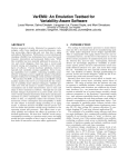
VarEMU: An Emulation Testbed for Variability-Aware
Table of Contents
ATHENA User's Manual