1
PLC2/30 Programmable Controller
Programming and Operations Manual
Important User Information
Because of the variety of uses for this equipment and because of the
differences between this solid state equipment and electromechanical
equipment, the user of and those responsible for applying this equipment
must satisfy themselves as to the acceptability of each application and
use of the equipment. In no event will Allen-Bradley Company, Inc. be
responsible or liable for indirect or consequential damages resulting from
the use or application of this equipment.
The illustrations, charts, and layout examples shown in this manual are
intended solely to illustrate the text of this manual. Because of the many
variables and requirements associated with any particular installation,
Allen-Bradley Company, Inc. cannot assume responsibility or liability for
actual use based upon the illustrative uses and applications.
No patent liability is assumed by Allen-Bradley Company, Inc. with
respect to use of information, circuits, equipment or software described in
this text.
Reproduction of the contents of this manual, in whole or in part, without
written permission of the Allen-Bradley Company, Inc. is prohibited.
1988 Allen-Bradley Company, Inc.
PLC is a registered trademark of Allen-Bradley Company, Inc.
WARNING: Warnings tell readers where people may be hurt if
procedures are not followed properly.
CAUTION: Cautions tell them where machinery may be
damaged or economic loss can occur if procedures are not
followed properly.
A Warning or Caution alerts you to:
a possible trouble spot
what causes the trouble to occur
the result of an improper action
how to avoid the situation
Table of Contents
Introduction . . . . . . . . . . . . . . . . . . . . . . . . . . . . . . . . . . . .
11
1.0 Introduction to This Manual . . . . . . . . . . . . . . . . . . . . . . . . . .
1.1 General . . . . . . . . . . . . . . . . . . . . . . . . . . . . . . . . . . . . . . . .
1.2 Capabilities . . . . . . . . . . . . . . . . . . . . . . . . . . . . . . . . . . . . .
1.2.1 Complementary I/O . . . . . . . . . . . . . . . . . . . . . . . . . . . . . .
1.2.2 Data Highway Compatibility . . . . . . . . . . . . . . . . . . . . . . . . .
1.2.3 Industrial Terminal Compatibility . . . . . . . . . . . . . . . . . . . . .
1.3 Additional Publications . . . . . . . . . . . . . . . . . . . . . . . . . . . . .
1.4 Terms Used in This Manual . . . . . . . . . . . . . . . . . . . . . . . . . .
11
11
13
14
14
14
15
16
Hardware Considerations . . . . . . . . . . . . . . . . . . . . . . . . .
21
2.0 General . . . . . . . . . . . . . . . . . . . . . . . . . . . . . . . . . . . . . . . .
2.1 Mode Select Switch . . . . . . . . . . . . . . . . . . . . . . . . . . . . . . .
2.2 Memory Write Protect . . . . . . . . . . . . . . . . . . . . . . . . . . . . . .
2.3 RunTime Errors . . . . . . . . . . . . . . . . . . . . . . . . . . . . . . . . . .
2.4 Processor Diagnostic Indicators . . . . . . . . . . . . . . . . . . . . . . .
2.5 PowerUp Recovery . . . . . . . . . . . . . . . . . . . . . . . . . . . . . . .
2.6 Switch Group Assembly . . . . . . . . . . . . . . . . . . . . . . . . . . . .
2.6.1 Last State Switch . . . . . . . . . . . . . . . . . . . . . . . . . . . . . . . .
2.6.2 I/O Rack Number . . . . . . . . . . . . . . . . . . . . . . . . . . . . . . . .
2.7 Industrial Terminal . . . . . . . . . . . . . . . . . . . . . . . . . . . . . . . .
2.8 Local System Structure . . . . . . . . . . . . . . . . . . . . . . . . . . . . .
2.9 Remote System Structure . . . . . . . . . . . . . . . . . . . . . . . . . . .
2.10 Local/Remote System Structure . . . . . . . . . . . . . . . . . . . . . .
2.11 Hardware Addressing Modes . . . . . . . . . . . . . . . . . . . . . . . .
2.12 Auxiliary Power Supplies . . . . . . . . . . . . . . . . . . . . . . . . . . .
2.12.1 1771P2 Auxiliary Power Supply . . . . . . . . . . . . . . . . . . . .
2.12.2 1777P2 Auxiliary Power Supply . . . . . . . . . . . . . . . . . . . .
2.12.3 1771P3, P4, and P5 Slot Power Supplies . . . . . . . . . . . .
2.12.4 1771P7 Power Supply . . . . . . . . . . . . . . . . . . . . . . . . . . .
2.12.5 1771PSC Power Supply Chassis . . . . . . . . . . . . . . . . . . .
21
21
22
23
24
25
25
26
26
27
27
28
29
210
210
210
211
211
211
211
Data Table . . . . . . . . . . . . . . . . . . . . . . . . . . . . . . . . . . . . .
31
3.0 General . . . . . . . . . . . . . . . . . . . . . . . . . . . . . . . . . . . . . . . .
3.1 Memory Structure . . . . . . . . . . . . . . . . . . . . . . . . . . . . . . . . .
3.2 Memory Organization . . . . . . . . . . . . . . . . . . . . . . . . . . . . . .
3.2.1 Data Table . . . . . . . . . . . . . . . . . . . . . . . . . . . . . . . . . . . . .
3.2.2 User Program . . . . . . . . . . . . . . . . . . . . . . . . . . . . . . . . . .
3.2.3 Message Storage Area . . . . . . . . . . . . . . . . . . . . . . . . . . . .
3.3 Hardware/Program Interface . . . . . . . . . . . . . . . . . . . . . . . . .
3.3.1 Image Tables . . . . . . . . . . . . . . . . . . . . . . . . . . . . . . . . . . .
31
31
32
32
316
317
317
317
ii
Table of Contents
3.3.2 Instruction Address . . . . . . . . . . . . . . . . . . . . . . . . . . . . . .
3.3.3 Fundamental Operation . . . . . . . . . . . . . . . . . . . . . . . . . . .
3.4 Data Table Documentation Forms . . . . . . . . . . . . . . . . . . . . .
3.4.1 Data Table Word Map (1024 Word) . . . . . . . . . . . . . . . . . . .
3.4.2 Data Table Map (128 Word) . . . . . . . . . . . . . . . . . . . . . . . .
3.4.3 Data Table Word Assignments (64 Word) . . . . . . . . . . . . . . .
3.4.4 Data Table Bit Assignments . . . . . . . . . . . . . . . . . . . . . . . .
3.4.5 Sequencer Table Bit Assignments . . . . . . . . . . . . . . . . . . . .
3.4.6 I/O Assignments . . . . . . . . . . . . . . . . . . . . . . . . . . . . . . . .
3.4.7 Timer/Counter Assignments . . . . . . . . . . . . . . . . . . . . . . . .
3.4.8 Data Storage Assignments . . . . . . . . . . . . . . . . . . . . . . . . .
318
321
323
323
324
325
326
327
328
329
329
Introduction to Programming . . . . . . . . . . . . . . . . . . . . . . .
41
4.0 General . . . . . . . . . . . . . . . . . . . . . . . . . . . . . . . . . . . . . . . .
4.1 Notational Conventions . . . . . . . . . . . . . . . . . . . . . . . . . . . . .
4.2 Ladder Diagram Logic . . . . . . . . . . . . . . . . . . . . . . . . . . . . . .
4.3 RelayType Instructions . . . . . . . . . . . . . . . . . . . . . . . . . . . . .
4.3.1 Examine Instructions . . . . . . . . . . . . . . . . . . . . . . . . . . . . .
4.3.2 Output Instructions . . . . . . . . . . . . . . . . . . . . . . . . . . . . . . .
4.3.3 Branch Instructions . . . . . . . . . . . . . . . . . . . . . . . . . . . . . .
4.3.4 Ending a Program . . . . . . . . . . . . . . . . . . . . . . . . . . . . . . .
4.3.5 Programming RelayType Instructions . . . . . . . . . . . . . . . . .
4.4 Operating Instructions . . . . . . . . . . . . . . . . . . . . . . . . . . . . . .
4.4.1 Addressing . . . . . . . . . . . . . . . . . . . . . . . . . . . . . . . . . . . .
4.4.2 Help Directories . . . . . . . . . . . . . . . . . . . . . . . . . . . . . . . . .
4.4.3 Searching . . . . . . . . . . . . . . . . . . . . . . . . . . . . . . . . . . . . .
4.4.4 Editing . . . . . . . . . . . . . . . . . . . . . . . . . . . . . . . . . . . . . . .
4.4.5 OnLine Programming . . . . . . . . . . . . . . . . . . . . . . . . . . . .
4.4.6 Clearing Memory . . . . . . . . . . . . . . . . . . . . . . . . . . . . . . . .
4.5 Program Recommendations . . . . . . . . . . . . . . . . . . . . . . . . .
41
41
42
43
43
45
49
412
413
414
415
415
416
419
423
430
432
Timer and Counter Instructions . . . . . . . . . . . . . . . . . . . . .
51
5.0 General . . . . . . . . . . . . . . . . . . . . . . . . . . . . . . . . . . . . . . . .
5.1 Timer Instructions . . . . . . . . . . . . . . . . . . . . . . . . . . . . . . . . .
5.1.1 Timer OnDelay Instruction . . . . . . . . . . . . . . . . . . . . . . . . .
5.1.2 Timer OffDelay Instruction . . . . . . . . . . . . . . . . . . . . . . . . .
5.1.3 Retentive Timer Instruction . . . . . . . . . . . . . . . . . . . . . . . . .
5.1.4 Retentive Timer Reset Instruction . . . . . . . . . . . . . . . . . . . .
5.1.5 Timer Accuracy for 10ms Timers . . . . . . . . . . . . . . . . . . . . .
5.2 Counter Instructions . . . . . . . . . . . . . . . . . . . . . . . . . . . . . . .
5.2.1 UpCounter Instruction . . . . . . . . . . . . . . . . . . . . . . . . . . . .
5.2.2 Counter Reset Instruction . . . . . . . . . . . . . . . . . . . . . . . . . .
5.2.3 DownCounter Instruction . . . . . . . . . . . . . . . . . . . . . . . . . .
5.2.4 Scan Counter Instruction . . . . . . . . . . . . . . . . . . . . . . . . . .
5.3 Cascading Timers or Counters . . . . . . . . . . . . . . . . . . . . . . . .
51
52
53
55
56
58
58
58
59
511
512
513
514
Table of Contents
iii
5.4 Programming Timer and Counter Instructions . . . . . . . . . . . . .
5.5 Scan Time and Instruction Execution Times . . . . . . . . . . . . . .
5.5.1 Scan Time . . . . . . . . . . . . . . . . . . . . . . . . . . . . . . . . . . . . .
5.5.2 Program for Determining Scan Time . . . . . . . . . . . . . . . . . .
5.6 Instruction Execution Time . . . . . . . . . . . . . . . . . . . . . . . . . . .
5.6.1 Relay Type, Timer and Counter, Data Manipulations,
Arithmetic, Output Override and I/O Update, Jump, and
Subroutine Instructions . . . . . . . . . . . . . . . . . . . . . . . . . . . . .
5.6.2
WordtoFile, Sequencers, FIFO, Word and Bit Shifts, File
Diagnostic, File Search, and Block Transfer Instructions . . . . . .
5.6.3 FiletoFile Move and File Complement . . . . . . . . . . . . . . . .
5.6.4 Logic Instructions FiletoFile AND, OR, XOR . . . . . . . . . . . .
514
517
517
518
519
520
522
523
Data Manipulation Instructions . . . . . . . . . . . . . . . . . . . . .
61
6.0 General . . . . . . . . . . . . . . . . . . . . . . . . . . . . . . . . . . . . . . . .
6.1 Data Transfer Instructions . . . . . . . . . . . . . . . . . . . . . . . . . . .
6.1.1 Get Instruction . . . . . . . . . . . . . . . . . . . . . . . . . . . . . . . . . .
6.1.2 Put Instruction . . . . . . . . . . . . . . . . . . . . . . . . . . . . . . . . . .
6.2 Data Comparison Instructions . . . . . . . . . . . . . . . . . . . . . . . .
6.2.1 Les and Equ Instructions . . . . . . . . . . . . . . . . . . . . . . . . . .
6.2.2 Get Byte and Limit Test Instructions . . . . . . . . . . . . . . . . . . .
6.2.3 Get Byte-Put Instruction . . . . . . . . . . . . . . . . . . . . . . . . . . .
6.3 Programming Data Manipulation Instructions . . . . . . . . . . . . . .
6.4 Arithmetic Instructions . . . . . . . . . . . . . . . . . . . . . . . . . . . . . .
6.4.1 Add Instruction . . . . . . . . . . . . . . . . . . . . . . . . . . . . . . . . .
6.4.2 Subtract Instruction . . . . . . . . . . . . . . . . . . . . . . . . . . . . . .
6.4.3 Multiply Instruction . . . . . . . . . . . . . . . . . . . . . . . . . . . . . . .
6.4.4 Divide Instruction . . . . . . . . . . . . . . . . . . . . . . . . . . . . . . . .
6.5 Programming Arithmetic Instructions . . . . . . . . . . . . . . . . . . .
6.6 BCD to Binary Conversion . . . . . . . . . . . . . . . . . . . . . . . . . . .
6.6.1 Programming a BCD to Binary Conversion Instruction . . . . . .
6.7 BinarytoBCD Conversion . . . . . . . . . . . . . . . . . . . . . . . . . .
6.7.1 Programming a Binaryto BCD Conversion Instruction . . . . .
61
62
62
63
64
64
67
68
69
611
612
613
614
614
615
616
617
618
618
Output Override and I/O Update Instructions . . . . . . . . . . .
71
7.0 General . . . . . . . . . . . . . . . . . . . . . . . . . . . . . . . . . . . . . . . .
7.1 Output Overrides . . . . . . . . . . . . . . . . . . . . . . . . . . . . . . . . .
7.2 I/O Updates . . . . . . . . . . . . . . . . . . . . . . . . . . . . . . . . . . . . .
7.2.1 Scan Sequence . . . . . . . . . . . . . . . . . . . . . . . . . . . . . . . . .
7.2.2 Immediate Input Instruction . . . . . . . . . . . . . . . . . . . . . . . . .
7.2.3 Immediate Output Instruction . . . . . . . . . . . . . . . . . . . . . . . .
7.3 Programming Immediate I/O Instructions . . . . . . . . . . . . . . . . .
7.4 Remote Fault Zone Programming . . . . . . . . . . . . . . . . . . . . . .
7.4.1 Dependent Programming . . . . . . . . . . . . . . . . . . . . . . . . . .
71
71
73
73
75
76
78
79
712
519
iv
Table of Contents
7.4.2 Independent Programming . . . . . . . . . . . . . . . . . . . . . . . . .
7.5 I/O Update Times . . . . . . . . . . . . . . . . . . . . . . . . . . . . . . . . .
7.5.1 Local Systems . . . . . . . . . . . . . . . . . . . . . . . . . . . . . . . . . .
7.5.2 Remote Systems . . . . . . . . . . . . . . . . . . . . . . . . . . . . . . . .
7.6 Watchdog Timer . . . . . . . . . . . . . . . . . . . . . . . . . . . . . . . . . .
713
715
715
715
716
Peripheral Functions . . . . . . . . . . . . . . . . . . . . . . . . . . . . .
81
8.0 General . . . . . . . . . . . . . . . . . . . . . . . . . . . . . . . . . . . . . . . .
8.1 Communication Rate Setting . . . . . . . . . . . . . . . . . . . . . . . . .
8.2 Contact Histogram . . . . . . . . . . . . . . . . . . . . . . . . . . . . . . . .
8.3 Digital Cassette Recorder . . . . . . . . . . . . . . . . . . . . . . . . . . .
8.3.1 Dumping Memory Content to Cassette Tape . . . . . . . . . . . . .
8.3.2 Loading Memory from Cassette Tape . . . . . . . . . . . . . . . . . .
8.3.3 Verification . . . . . . . . . . . . . . . . . . . . . . . . . . . . . . . . . . . .
8.3.4 Program Verification . . . . . . . . . . . . . . . . . . . . . . . . . . . . . .
8.3.5 Displaying and Locating Errors . . . . . . . . . . . . . . . . . . . . . .
8.4 Data Cartridge Recorder . . . . . . . . . . . . . . . . . . . . . . . . . . . .
8.4.1 Dumping Memory Content onto Data Cartridge Tape . . . . . . .
8.4.2 Loading Memory from a Data Cartridge Tape . . . . . . . . . . . .
8.4.3 Data Cartridge Verification . . . . . . . . . . . . . . . . . . . . . . . . .
8.5 Ladder Diagram Dump . . . . . . . . . . . . . . . . . . . . . . . . . . . . .
8.6 Total Memory Dump . . . . . . . . . . . . . . . . . . . . . . . . . . . . . . .
81
81
82
84
84
84
85
85
86
86
86
87
88
88
88
Report Generation . . . . . . . . . . . . . . . . . . . . . . . . . . . . . . .
91
9.0 General . . . . . . . . . . . . . . . . . . . . . . . . . . . . . . . . . . . . . . . .
9.1 Report Generation Commands . . . . . . . . . . . . . . . . . . . . . . .
9.1.1 Message Control Word File - MS, 0 . . . . . . . . . . . . . . . . . . .
9.1.2 Message Store - MS . . . . . . . . . . . . . . . . . . . . . . . . . . . . .
9.1.3 Message Print - MP . . . . . . . . . . . . . . . . . . . . . . . . . . . . . .
9.1.4 Message Report - MR . . . . . . . . . . . . . . . . . . . . . . . . . . . .
9.1.5 Message Delete - MD . . . . . . . . . . . . . . . . . . . . . . . . . . . .
9.1.6 Message Index - MI . . . . . . . . . . . . . . . . . . . . . . . . . . . . . .
9.1.7 Control Codes and Special Commands . . . . . . . . . . . . . . . .
9.2 Manually Initiated Report Generation . . . . . . . . . . . . . . . . . . .
9.3 Automatic Report Generation . . . . . . . . . . . . . . . . . . . . . . . . .
9.3.1 Messages 16 . . . . . . . . . . . . . . . . . . . . . . . . . . . . . . . . . .
9.3.2 Additional Messages . . . . . . . . . . . . . . . . . . . . . . . . . . . . .
9.3.3 Example Programming . . . . . . . . . . . . . . . . . . . . . . . . . . . .
91
93
94
95
96
97
97
97
97
911
912
913
913
914
Block Transfer . . . . . . . . . . . . . . . . . . . . . . . . . . . . . . . . . .
101
10.0 General . . . . . . . . . . . . . . . . . . . . . . . . . . . . . . . . . . . . . . .
10.1 Basic Operation . . . . . . . . . . . . . . . . . . . . . . . . . . . . . . . . .
10.2 Block Transfer Instructions . . . . . . . . . . . . . . . . . . . . . . . . .
10.2.1 Data Address and Module Address . . . . . . . . . . . . . . . . . .
101
101
104
104
Table of Contents
v
10.2.2 Block Length . . . . . . . . . . . . . . . . . . . . . . . . . . . . . . . . . .
10.2.3 File Address . . . . . . . . . . . . . . . . . . . . . . . . . . . . . . . . . .
10.2.4 Enable Bit and Done Bit . . . . . . . . . . . . . . . . . . . . . . . . . .
10.3 Instruction Notes for Block Transfer Read and
Write Instructions . . . . . . . . . . . . . . . . . . . . . . . . . . . . . . . . .
10.4 Causes of RunTime Errors . . . . . . . . . . . . . . . . . . . . . . . . .
10.5 Programming Block Transfer Read and Write Instructions . . .
10.6 Multiple Reads of Different Block Lengths from One Module . .
10.7 Defining the Block Transfer Data Address Area . . . . . . . . . . .
10.8 Buffering Data . . . . . . . . . . . . . . . . . . . . . . . . . . . . . . . . . .
10.9 Bidirectional Block Transfer . . . . . . . . . . . . . . . . . . . . . . . . .
10.9.1 Operation . . . . . . . . . . . . . . . . . . . . . . . . . . . . . . . . . . . .
10.9.2 Data Address and Module Address . . . . . . . . . . . . . . . . . .
10.9.3 File Address . . . . . . . . . . . . . . . . . . . . . . . . . . . . . . . . . .
10.9.4 Block Length . . . . . . . . . . . . . . . . . . . . . . . . . . . . . . . . . .
10.9.5 Programming Considerations . . . . . . . . . . . . . . . . . . . . . .
105
105
106
106
106
106
108
1011
1012
1014
1014
1017
1017
1017
1018
Jump Instructions and Subroutine Programming . . . . . . . .
111
11.0 General . . . . . . . . . . . . . . . . . . . . . . . . . . . . . . . . . . . . . . .
11.1 Jump Instruction . . . . . . . . . . . . . . . . . . . . . . . . . . . . . . . . .
11.1.1 Programming Jump/ Subroutine Instructions . . . . . . . . . . . .
11.1.2 Multiple Jumps to the Same Label . . . . . . . . . . . . . . . . . . .
11.2 Label Instruction . . . . . . . . . . . . . . . . . . . . . . . . . . . . . . . . .
11.3 Jump to Subroutine Instruction . . . . . . . . . . . . . . . . . . . . . . .
11.3.1 Subroutine Area . . . . . . . . . . . . . . . . . . . . . . . . . . . . . . . .
11.3.2 Nested Subroutines . . . . . . . . . . . . . . . . . . . . . . . . . . . . .
11.3.3 Recursive Subroutine (Looping) Calls . . . . . . . . . . . . . . . .
11.3.4 Subroutine Programming Considerations . . . . . . . . . . . . . .
11.4 Return Instruction . . . . . . . . . . . . . . . . . . . . . . . . . . . . . . . .
111
111
113
113
116
117
1110
1111
1112
1112
1114
Data Transfer File Instructions . . . . . . . . . . . . . . . . . . . . . .
121
12.0 General . . . . . . . . . . . . . . . . . . . . . . . . . . . . . . . . . . . . . . .
12.1 File Concepts . . . . . . . . . . . . . . . . . . . . . . . . . . . . . . . . . . .
12.1.1 File Definition . . . . . . . . . . . . . . . . . . . . . . . . . . . . . . . . . .
12.1.2 File Planning . . . . . . . . . . . . . . . . . . . . . . . . . . . . . . . . . .
12.1.3 File Instructions . . . . . . . . . . . . . . . . . . . . . . . . . . . . . . . .
12.1.4 Programming File Instructions . . . . . . . . . . . . . . . . . . . . . .
12.1.5 File Instruction RunTime Error . . . . . . . . . . . . . . . . . . . . .
12.2 FiletoFile Move . . . . . . . . . . . . . . . . . . . . . . . . . . . . . . . . .
12.2.1 Programming FiletoFile Move Instructions . . . . . . . . . . . .
12.3 FiletoWord Move . . . . . . . . . . . . . . . . . . . . . . . . . . . . . . .
12.3.1 Programming FiletoWord Move Instructions . . . . . . . . . . .
12.4 WordtoFile Move . . . . . . . . . . . . . . . . . . . . . . . . . . . . . . .
12.4.1 Programming WordtoFile Move Instructions . . . . . . . . . . .
12.5 Data Monitor Mode . . . . . . . . . . . . . . . . . . . . . . . . . . . . . . .
121
121
121
122
122
1211
1212
1212
1214
1215
1216
1218
1219
1221
vi
Table of Contents
12.5.1 Accessing the Data Monitor Mode . . . . . . . . . . . . . . . . . . .
12.5.2 Data Monitor Display . . . . . . . . . . . . . . . . . . . . . . . . . . . .
12.5.3 Cursor Controls . . . . . . . . . . . . . . . . . . . . . . . . . . . . . . . .
12.5.4 Data Monitoring Procedures . . . . . . . . . . . . . . . . . . . . . . .
12.5.5 Entering and Changing Data . . . . . . . . . . . . . . . . . . . . . . .
1221
1224
1225
1226
1227
Shift Register Instructions . . . . . . . . . . . . . . . . . . . . . . . . .
131
13.0 General . . . . . . . . . . . . . . . . . . . . . . . . . . . . . . . . . . . . . . .
13.1 Shift File Up . . . . . . . . . . . . . . . . . . . . . . . . . . . . . . . . . . . .
13.1.1 Programming Shift File Up Instruction . . . . . . . . . . . . . . . .
13.2 Shift File Down . . . . . . . . . . . . . . . . . . . . . . . . . . . . . . . . . .
13.2.1 Programming Shift File Down Instruction . . . . . . . . . . . . . .
13.3 FIFO Load and FIFO Unload . . . . . . . . . . . . . . . . . . . . . . . .
13.3.1 Programming FIFO Load and FIFO Unload Instruction . . . . .
131
132
133
135
135
136
138
Bit Shifts . . . . . . . . . . . . . . . . . . . . . . . . . . . . . . . . . . . . . .
141
14.0 General . . . . . . . . . . . . . . . . . . . . . . . . . . . . . . . . . . . . . . .
14.1 Bit Shift Left . . . . . . . . . . . . . . . . . . . . . . . . . . . . . . . . . . . .
14.1.1 Programming Bit Shift Left Instruction . . . . . . . . . . . . . . . . .
14.2 Bit Shift Right . . . . . . . . . . . . . . . . . . . . . . . . . . . . . . . . . . .
14.2.1 Programming Bit Shift Right Instruction . . . . . . . . . . . . . . .
14.3 Examine Off Shift Bit . . . . . . . . . . . . . . . . . . . . . . . . . . . . . .
14.3.1 Programming Examine Off Shift Bit Instruction . . . . . . . . . .
14.4 Examine On Shift Bit . . . . . . . . . . . . . . . . . . . . . . . . . . . . . .
14.4.1 Programming Examine On Shift Bit Instruction . . . . . . . . . .
14.5 Set Shift Bit . . . . . . . . . . . . . . . . . . . . . . . . . . . . . . . . . . . .
14.5.1 Programming Set Shift Bit Instruction . . . . . . . . . . . . . . . . .
14.6 Reset Shift Bit . . . . . . . . . . . . . . . . . . . . . . . . . . . . . . . . . . .
14.6.1 Programming Reset Shift Bit Instruction . . . . . . . . . . . . . . .
141
141
143
145
146
146
146
148
148
149
149
1410
1411
Sequencer Instructions . . . . . . . . . . . . . . . . . . . . . . . . . . .
151
15.0 General . . . . . . . . . . . . . . . . . . . . . . . . . . . . . . . . . . . . . . .
15.1 Sequencer Output Instruction . . . . . . . . . . . . . . . . . . . . . . . .
15.1.1 Sequencer Output Analogy . . . . . . . . . . . . . . . . . . . . . . . .
15.1.2 Operation of the Sequencer Output Instruction . . . . . . . . . .
15.1.3 Masking Output Data . . . . . . . . . . . . . . . . . . . . . . . . . . . .
15.1.4 Instruction Overview . . . . . . . . . . . . . . . . . . . . . . . . . . . . .
15.1.5 Programming the Sequencer Output Instruction . . . . . . . . .
15.2 Sequencer Input Instruction . . . . . . . . . . . . . . . . . . . . . . . . .
15.2.1 Operation of the Sequencer Input Instruction . . . . . . . . . . .
15.2.2 Masking Input Data . . . . . . . . . . . . . . . . . . . . . . . . . . . . .
15.2.3 Instruction Overview . . . . . . . . . . . . . . . . . . . . . . . . . . . . .
15.2.4 Programming the Sequencer Input Instruction . . . . . . . . . . .
15.3 Sequencer Load Instruction . . . . . . . . . . . . . . . . . . . . . . . . .
151
153
153
154
155
156
156
1510
1510
1510
1510
1511
1513
Table of Contents
vii
15.3.1 Operation of the Sequencer Load Instruction . . . . . . . . . . .
15.3.2 Instruction Overview . . . . . . . . . . . . . . . . . . . . . . . . . . . . .
15.3.3 Programming the Sequencer Load Instruction . . . . . . . . . .
1513
1514
1514
File Logic Instructions . . . . . . . . . . . . . . . . . . . . . . . . . . . .
161
16.0 General . . . . . . . . . . . . . . . . . . . . . . . . . . . . . . . . . . . . . . .
16.1 FiletoFile Logic Instructions . . . . . . . . . . . . . . . . . . . . . . . .
16.1.1 FiletoFile AND . . . . . . . . . . . . . . . . . . . . . . . . . . . . . . . .
16.1.2 FiletoFile OR . . . . . . . . . . . . . . . . . . . . . . . . . . . . . . . . .
16.1.3 FiletoFile XOR . . . . . . . . . . . . . . . . . . . . . . . . . . . . . . . .
16.1.4 File Complement . . . . . . . . . . . . . . . . . . . . . . . . . . . . . . .
16.2 WordtoFile Logic Instructions . . . . . . . . . . . . . . . . . . . . . . .
16.2.1 WordtoFile AND . . . . . . . . . . . . . . . . . . . . . . . . . . . . . . .
16.2.2 WordtoFile OR . . . . . . . . . . . . . . . . . . . . . . . . . . . . . . . .
16.2.3 WordtoFile XOR . . . . . . . . . . . . . . . . . . . . . . . . . . . . . .
161
161
162
164
165
166
168
169
1611
1612
File Search and File Diagnostic Instructions . . . . . . . . . . .
171
17.0 General . . . . . . . . . . . . . . . . . . . . . . . . . . . . . . . . . . . . . . .
17.1 File Search . . . . . . . . . . . . . . . . . . . . . . . . . . . . . . . . . . . . .
17.2 File Diagnostics . . . . . . . . . . . . . . . . . . . . . . . . . . . . . . . . .
171
171
174
Troubleshooting Aids . . . . . . . . . . . . . . . . . . . . . . . . . . . .
181
18.0 General . . . . . . . . . . . . . . . . . . . . . . . . . . . . . . . . . . . . . . .
18.1 Bit Manipulation and Monitor . . . . . . . . . . . . . . . . . . . . . . . .
18.1.1 Bit Manipulation . . . . . . . . . . . . . . . . . . . . . . . . . . . . . . . .
18.1.2 Bit Monitor . . . . . . . . . . . . . . . . . . . . . . . . . . . . . . . . . . . .
18.2 Force On and Force Off Functions . . . . . . . . . . . . . . . . . . . .
18.3 Forced Address Display . . . . . . . . . . . . . . . . . . . . . . . . . . .
18.4 Temporary End Instruction . . . . . . . . . . . . . . . . . . . . . . . . . .
18.5 ERR Message for an Illegal OP Code . . . . . . . . . . . . . . . . . .
181
182
182
183
183
184
185
185
Special Programming Techniques . . . . . . . . . . . . . . . . . . .
191
19.0 General . . . . . . . . . . . . . . . . . . . . . . . . . . . . . . . . . . . . . . .
19.1 One Shot . . . . . . . . . . . . . . . . . . . . . . . . . . . . . . . . . . . . . .
19.1.1 Leading Edge OneShot . . . . . . . . . . . . . . . . . . . . . . . . . .
19.1.2 Trailing Edge OneShot . . . . . . . . . . . . . . . . . . . . . . . . . .
191
191
191
192
Addressing . . . . . . . . . . . . . . . . . . . . . . . . . . . . . . . . . . . .
A1
A.0 Appendix Objectives . . . . . . . . . . . . . . . . . . . . . . . . . . . . . . .
A.1 Addressing Your Hardware . . . . . . . . . . . . . . . . . . . . . . . . . .
A.2 Addressing Modes . . . . . . . . . . . . . . . . . . . . . . . . . . . . . . . .
A.2.1 2Slot Addressing . . . . . . . . . . . . . . . . . . . . . . . . . . . . . . .
A.2.2 1Slot Addressing . . . . . . . . . . . . . . . . . . . . . . . . . . . . . . .
A1
A1
A2
A3
A8
viii
Table of Contents
A.2.3 1/2Slot Addressing . . . . . . . . . . . . . . . . . . . . . . . . . . . . . .
A.3 System Configurations . . . . . . . . . . . . . . . . . . . . . . . . . . . . .
A11
A16
Number Systems . . . . . . . . . . . . . . . . . . . . . . . . . . . . . . . .
B1
B.0 General . . . . . . . . . . . . . . . . . . . . . . . . . . . . . . . . . . . . . . . .
B.1 Decimal Numbering System . . . . . . . . . . . . . . . . . . . . . . . . .
B.2 Octal Numbering System . . . . . . . . . . . . . . . . . . . . . . . . . . .
B.3 Binary Numbering System . . . . . . . . . . . . . . . . . . . . . . . . . . .
B.3.1 Binary Coded Decimal . . . . . . . . . . . . . . . . . . . . . . . . . . . .
B.3.2 Binary Coded Octal . . . . . . . . . . . . . . . . . . . . . . . . . . . . . .
B.4 Hexadecimal Numbering System . . . . . . . . . . . . . . . . . . . . . .
B1
B1
B2
B3
B4
B5
B6
Programming .01Second Timers . . . . . . . . . . . . . . . . . . . .
C1
C.0 Introduction . . . . . . . . . . . . . . . . . . . . . . . . . . . . . . . . . . . . .
C.1 Time Base Selection . . . . . . . . . . . . . . . . . . . . . . . . . . . . . . .
C.2 Timer Accuracy . . . . . . . . . . . . . . . . . . . . . . . . . . . . . . . . . .
C.3 10Msec Timers - Typical Applications . . . . . . . . . . . . . . . . . .
C.4 Hardware/Processor Considerations . . . . . . . . . . . . . . . . . . .
C.5 10Msec Timers - Programming Techniques . . . . . . . . . . . . .
C.5.1 Scan Time . . . . . . . . . . . . . . . . . . . . . . . . . . . . . . . . . . . .
C.5.2 Program Execution . . . . . . . . . . . . . . . . . . . . . . . . . . . . . .
C.5.3 Programming Compensation . . . . . . . . . . . . . . . . . . . . . . .
C.6 Program ScanTime Computation . . . . . . . . . . . . . . . . . . . . .
C1
C1
C2
C4
C5
C5
C6
C6
C7
C9
Chapter
1
Introduction
1.0
Introduction to This Manual
This manual presents the information you need to program and operate
your Allen-Bradley PLC-2/30 Programmable Controller.
After reading this manual, you should be able to:
establish system configurations consisting of:
-
scanners
interface modules
input modules
output modules
power supplies
program:
-
timers
counters
extended arithmetic functions
relay-type functions
and data transfer, for a few examples.
This manual is your entry into understanding the PLC-2/30 programmable
controller.
To find what the topics are in the individual chapters — Use the Table of
Contents.
To get an overview of what that chapter presents — Look in the
“General” section of each chapter.
To get a better understanding of slot addressing — Use the Appendix.
To find where a specific item is located in the text — Use the Index.
1.1
General
The PLC-2/30 programmable controller consists of:
The 1772-LP3 processor
An I/O structure (I/O chassis containing I/O modules)
11
Chapter 1
Introduction
With a user-written program and appropriate I/O modules, the PLC-2/30
programmable controller can be used to control many types of industrial
applications such as:
Process control
Material handling
Palletizing
Measurement and gauging
Pollution control and monitoring
The 1772-LP3 processor has a read/write CMOS memory that stores user
program instructions, numeric values and I/O device status. The user
program is a set of instructions in a particular order that describes the
operations to be performed and the operating conditions. It is entered into
memory, rung by rung, in a ladder diagram and functional block display
format from the keyboard of a 1770-T3 or 1784–T50 terminal. The ladder
diagram symbols closely resemble the relay symbols used in hardwired
relay control systems. The functional block displays are an easy method of
programming and monitoring advanced instructions.
During program operation, the PLC-2/30 processor continuously monitors
the status of input devices and, based on user program instructions,
either energizes or de–energizes output devices. Because the memory is
programmable, the user program can be readily changed if required by the
application.
The PLC-2/30 processor’s functions include:
Relay-type functions (Examine On, Examine Off, Output Energize,
Output Latch, Output Unlatch and Branching)
Complete forced I/O
Data transfer
Data comparison
Three-digit, four-function arithmetic (+, –, ×, :–) :–:–
Timing functions: On-Delay and Off-Delay, Retentive and Nonretentive
with time bases of 1.0, 0.1 and 0.01 seconds (timing range 0.02 to 999
seconds).
Bidirectional counting (up or down) with a range of 0 to 999 counts.
Self-monitoring/diagnostic capabilities
Expandable data table
Memory capacity of 16,256 words
896 I/O device capacity is available in local or remote configurations.
896 inputs and 896 outputs when used with specific configurations.
Memory write protect
Program control instructions
- Jump
- Subroutines
12
Chapter 1
Introduction
Functional Block Instructions
- Shift Register instructions
- File-to-File and Word-to-File Logic instructions
- File-to-File, Word-to-File and File-to-Word transfer instructions
Binary to BCD and BCD to Binary conversions
On-line programming
Data Highway and Data Highway II compatible
Sequencers
Contact histogram
Report generation
1.2
Capabilities
The data table for the 1772-LP3 processor can be expanded to 8,064 words
with an 8K memory or to 8,192 words with a 16K memory. However, an
8,064 word data table is impractical with an 8K memory since there would
be nothing available for the user program.
You can expand the data table from the default size of 128 words (1 rack)
to 256 words (2 racks, word address 3778) in 2-word increments. From
word address 4008 on, the data table must be expanded in 128-word
sections. The I/O image tables, therefore, can be configured in size from
1 to 7 I/O racks. Each rack added, above one, increments by 108 the first
available address for timers and counters. Table 1.A lists the first available
timer/counter address when different numbers of racks are selected.
In addition, the processor can control up to 896 inputs and 896 outputs
for a total of 1,792 I/O points in a remote system of seven 128 I/O racks
(Table 1.A).
Table 1.A
PLC2/30 Processor Capabilities (Cat. No. 1772LP3)
#I/O Racks
Max. I/O Points1 (decimal)
First Available T/C Address
(octal)
1
2
3
4
5
6
7
128
256
384
512
640
768
896
020
030
040
050
060
070
200
1 Without complementary I/O.
With complementary I/O, maximum I/O points is double the tabulated number up to 1,792.
13
Chapter 1
Introduction
1.2.1
Complementary I/O
When using a 1772-SD2 remote I/O scanner/distribution panel, the I/O
device capacity can be increased from 896 to 1,792 I/O. The increase is
accomplished through configuration of the racks and programming. For
more information, refer to the Remote I/O Scanner/Distribution Panel
Product Data (publication 1772-2.18).
1.2.2
Data Highway Compatibility
With the proper interface module, the PLC-2/30 processor can be
connected to the Allen-Bradley Data Highway or other industry standard
buses. Table 1.B lists several “from-to” possibilities and the Allen-Bradley
module used to accomplish that function.
Table 1.B
Interface Modules
Interface Locations From:
To:
Interface Module
PLC2/30
Data Highway
1771KA2
PLC2/30
Data Highway II
1779KP2
1779KP2R
PLC2/30
RS232
1771KG
1771KGM
1771KH
Data Highway
Non AB1
1771KE
1771KF
1770KF2
Data Highway
Fisher Provox
1771KX1
Data Highway II
Non AB1
1779KFL
1779KFM
1 Non AllenBradley implies using Data Highway or Data Highway II to communicate with industry standard devices.
individual product brochures for specific connectivity information.
1.2.3
Industrial Terminal
Compatibility
14
See the
Industrial Terminals (cat. no. 1770-T1 or -T2) can be used on a limited
basis to program a PLC-2/30 programmable controller. Be aware that
only features supported by these terminals may be entered. The 1770-T3
and 1784-T50 terminals provide full PLC-2/30 capability. Refer to the
Industrial Terminal System User’s Manual (publication 1770-6.5.3 or
1784-6.5.1) for details.
Chapter 1
Introduction
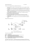
WARNING: Do not use a 1770-T1 or 1770-T2 industrial
terminal to edit or change a program or data table values
in PLC-2/30 memory that were generated using a 1770-T3
industrial terminal. Block instructions and instructions with
word addresses 4008 or greater will not be displayed properly
(Figure 1.1). The ERR message may appear randomly in the
user program at instructions and addresses that the -T1 and -T2
industrial terminals are not designed to handle. Changes to the
user program and/or data table with a -T1 or -T2 terminal could
result in unpredictable machine motion with possible damage to
equipment and/or injury to personnel.
Figure 1.1
ERR Message for Invalid Display of Processor Memory
113
][
14
1025
()
16
1770T3 Display (Actual content in processor memory)
11314
][
ERR
02516
()
1770T1 or T2 Display (Invalid display of processor memory)
1.3
Additional Publications
Additional information regarding PLC-2/30 programmable controller
components is available in:
PLC-2/20, PLC-2/30 Programmable Controller Assembly and
Installation Manual (publication 1772-6.6.2) contains necessary
information on installation, assembly, maintenance and troubleshooting.
Appendix C, Programming 0.01-Second Timers with the Mini-PLC-2
Programmable Controller.
15
Chapter 1
Introduction
1.4
Terms Used in This Manual
We use the following terms to describe the various parts of your PLC-2/30
system.
Chassis — a hardware assembly used to house PC devices such as I/O
modules, adapter modules, processor modules, power supplies and some
processors (PLC-2/02, -2/16 and -2/17, for example).
I/O Group — The logical assignment of a specific input image table
word and its companion output image table word to a rack location. For
example: address 123 indicates an input module in rack 2, I/O group 3.
This applies to all addressing modes.
Rack — an I/O addressing unit that corresponds to 8 input image table
words and 8 output image table words (128 input and 128 output
terminals).
Rack Fault — 1) The condition that occurs because of a loss of
communication between the processor and remote I/O chassis; 2) any
diagnostic indicator that lights up to signal a rack fault.
Slot — 1) The physical location where each module is placed within
a chassis; 2) a part of the Rack-Group-Slot addressing information for
intelligent I/O modules.
Slot Addressing — a method of assigning one input and one output image
table word to two slots, one slot, or one-half of a slot. (Appendix A is an
in-depth discussion on this topic.)
Slot Pair — two adjacent slots that can share image table words. Slot pairs
are: slots 0 and 1, 2 and 3, 4 and 5, and 6 and 7. (See Appendix A)
These and other terms are defined in Programmable Controller Terms
(publication no. PCGI–7.2).
16
Chapter
2
Hardware Considerations
2.0
General
This chapter describes only those hardware items required when
programming or operating the PLC-2/30 programmable controller. For
more complete hardware information, refer to the PLC-2/20, PLC-2/30
Programmable Controller Assembly and Installation Manual (publication
no. 1772-6.6.2).
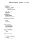
2.1
Mode Select Switch
A four-position mode select switch (Figure 2.1) is located on the front of
the processor. You can select one of four positions with this switch:
PROG — This switch position places the processor in the program
mode. It is used when instructions are entered into memory. They can be
entered from an industrial terminal, a 1770-SA digital cassette recorder
or a 1770-SB data cartridge recorder. All outputs are disabled when the
switch is in this position.
TEST — This switch position places the processor in the test mode. The
user program is tested under simulated operating conditions without
actually energizing any output devices. All outputs are disabled in this
switch position.
RUN — This switch position places the processor in the run mode.
The user program will be executed and outputs are controlled by the
program. Changes to the user program or data table are not permitted in
this switch position.
RUN/PROG — This switch position places the processor in the
run/program mode. The processor functions as it does in the RUN
position. In this position, you can cause the processor to go into the
program or test mode without having to turn the switch to that position.
On-line changes to the program and/or data table are allowed in this
position with 1770-T3 or 1784-T50 industrial terminals.
The key can be removed from the processor in any of the four switch
positions.
21
Chapter 2
Hardware Considerations
Figure 2.1
PLC2/30 Processor
Diagnostic
Indicators
2.2
Memory Write Protect
22
Keylock Mode
Select Switch
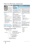
When the memory write protect jumper (Figure 2.2) is removed from a
1772-LH processor interface module, data table values can be changed
between word addresses 0108 and 3778. These values can be changed only
when the processor is in the program mode or in the run/program mode
using on-line data change.
Chapter 2
Hardware Considerations
Figure 2.2
Memory Write Protect Jumper
HALFTONE WITH CALLOUT
The remaining words in memory from 4008 to the end of memory,
including data table and user program, are protected and cannot be altered
by programming. The memory write protect feature guards against
unintentional changes to processor memory.
2.3
RunTime Errors
The processor and an industrial terminal can diagnose certain errors
occurring during the execution of the user program which result from
improper programming techniques. For example, it is possible to program
a series of instructions which require the processor to perform an operation
which it cannot do or perform an operation which is defined as illegal
(such as jump to a label that is not located closer to the end of program;
i.e., a jump backwards). These errors become apparent only while the
program is being executed, so are termed run-time errors. If a run-time
error occurs, the processor halts program execution and the PROCESSOR
FAULT indicator illuminates.
The first step in diagnosing run-time errors is to connect the industrial
terminal. It will display the message run-time error in the initial mode
select display. If the industrial terminal is already connected at the time
that a run-time error occurs, the ladder diagram is replaced by the mode
select display containing the error message. Run-time errors can be
detected by the industrial terminal when the processor is in either of two
23
Chapter 2
Hardware Considerations
modes, program or remote program. (If the keyswitch is in
RUN/PROGRAM position, the industrial terminal automatically puts
the processor into remote program mode. If the keyswitch is in the RUN
position, or when it is connected to the processor through the 1771-KA2
communications adapter module, you must manually change the keyswitch
to the PROGRAM position).
WARNING: Forces are immediately removed if a Run-time
error occurs.
After returning the industrial terminal display to ladder diagram mode by
pressing [1][1] in mode selection operation, the industrial terminal displays
the instruction that caused the error with a message describing the run-time
error.
After you have corrected the run-time error by editing the user program,
the processor can be restarted by switching to the run or run/program
mode.
2.4
Processor Diagnostic
Indicators
Five indicators are located on the front of the processor (Figure 2.1). You
should become familiar with these indicators.
MEMORY FAULT — Illuminates when an error in the parity of data
retrieved from memory is detected. Changing the mode select switch to
the PROG position or cycling line power may clear this fault condition.
Reloading the program may also clear the fault.
BATTERY LOW — When the batteries for memory back-up are low,
this red indicator flashes on and off. Alkaline batteries will continue
to back up memory for about one week after the BATTERY LOW
indicator begins to flash. Lithium batteries have a longer life, but are
essentially dead when the indicator flashes. Regular replacement of
the batteries is recommended: for alkaline, every 6 to 12 months; for
lithium, every 2 years. (See the Assembly and Installation manual for
replacement details, publication no. 1772-6.6.2.)
The low battery bit, bit 027/00, will cycle on and off when a low battery
voltage condition is detected and the mode select switch is not in the
PROG position. Programming techniques can be used to examine this
bit and to control some type of alerting device when a low battery
condition exists.
24
Chapter 2
Hardware Considerations
PROCESSOR FAULT — Illuminates when the logic circuits controlling
the processor scan fail or if processor error or run-time errors occur
which cause the processor to halt operation.
If the processor fault is a run-time error, the industrial terminal will
display RUN TIME ERROR when the keyswitch is in the PROGRAM
or RUN/PROGRAM position.
RUN — Illuminates when the processor is in the run or run/program
mode. It also indicates that outputs are being controlled by user
program.
DC ON — Illuminates when the 5.1V DC line to the logic circuitry in
the processor memory and I/O modules is satisfactory.
2.5
PowerUp Recovery
When local I/O racks are powered by 1771-P3, -P4, -P5 or -P7 power
supplies, the processor control module (Cat. No. 1772-LG) may experience
a problem with these racks.
Upon recovery from a power lock (momentary or otherwise), processors in
the RUN or TEST mode attempt to read the local racks before the power
supplies are ready. This leads to a processor fault. The fault may be
identified by the conditions of the indicators:
Indicators
1772LG Module
RUN
PROC FAULT
Series A, Rev. L
OFF
ON
Series A, Rev. K or earlier
OFF
OFF
If the problem occurs, put the keyswitch in the program load position, then
return to RUN, or cycle power to the processor.
2.6
Switch Group Assembly
A switch group assembly is located on the I/O chassis backplane. It is used
to control output behavior when a fault occurs, to identify the I/O rack
number for local systems and to identify the addressing mode for remote
systems.
The switch and its functions, when used in local racks, are shown in
Figure 2.3. In this setup, the PLC-2/30 is communicating with the I/O
chassis through a 1771-AL Local I/O Adapter module.
25
Chapter 2
Hardware Considerations
When using remote I/O (the 1772-SD2 scanner and the 1771-ASB remote
I/O Adapter), these switches will be set according to the adapter module’s
requirements.
2.6.1
Last State Switch
The last state switch (switch no. 1) on the 1771 I/O chassis must be
properly set. ON indicates that the outputs are left in their last state when
a fault is detected. Machine operation can continue after fault detection.
OFF indicates that the outputs are de-energized when a fault is detected. In
addition, in remote systems, the switches on the 1772-SD2 Remote I/O
Scanner/Distribution panel and the 1771-ASB Remote I/O Adapter
must be properly set. Refer to publications 1772-2.18 and 1771-6.5.37,
respectively, for information on their switch settings.
WARNING: Switch No. 1 of the 1771 I/O chassis should be set
to OFF for most applications. This allows the processor to turn
controlled devices off when a fault is detected. If this switch is
set to ON, machine operation can continue after fault detection.
Damage to equipment and/or injury to personnel could result.
2.6.2
I/O Rack Number
The setting of switches 3, 4 and 5 determines the I/O data table and
program address of the modules in this chassis — this is the local rack
number.
Improper setting of these switches will result in misdirected
communications between processor and the desired I/O rack.
26
Chapter 2
Hardware Considerations
Figure 2.3
1771 I/O Chassis Backplane Switch Settings for Local I/O Systems
No significance should be set to OFF
On:
Off:
Outputs remain in last state
when fault is detected.
Outputs deenergized when
fault is detected.
2.7
Industrial Terminal
Local
Rack
Numbers
3
4
5
1
2
3
4
5
6
7
On
On
On
On
Off
Off
Off
On
On
Off
Off
On
On
Off
On
Off
On
Off
On
Off
On
Switch
The 1770-T3 and 1784-T50 industrial terminals are the primary
programming terminals for the PLC-2/30 programmable controller. They
are used to load, edit, monitor and troubleshoot the user’s program in the
PLC-2/30 memory.
For detailed information about the 1770-T3 Industrial Terminal, refer to
the Industrial Terminal System User’s Manual, publication no. 1770-6.5.3.
For detailed information about the 1784-T50 Industrial Terminal, refer to
the Industrial Terminal T50 User’s Manual, publication no. 1784-6.5.1.
2.8
Local System Structure
A local system has the processor and each I/O chassis within 3-6 cable feet
of each other. Up to 7 local I/O racks may be assigned.
For proper transmission of data between the PLC-2/30 processor and
local bulletin 1771 I/O modules, the I/O chassis must contain a local I/O
Adapter Module (Cat. No. 1771-AL). The local adapter module must be
installed in each I/O chassis used with the processor. Diagnostic indicators
27
Chapter 2
Hardware Considerations
on the front panel of the local adapter module aid in troubleshooting. These
indicators are:
ACTIVE — Illuminates when proper communication is established
between the processor and the I/O chassis. It also indicates that DC
power is properly supplied to the I/O chassis. It is normally on.
RACK FAULT — Illuminates when I/O data is not in the proper format.
It is normally off.
Possible causes of a rack fault are:
Data parity error on address or control lines
Missing terminator plug
Disconnected/broken communications cable
No power at the processor.
An I/O Interconnect cable is required to connect between the PLC-2/30
and local I/O rack adapter modules. It is available in two sizes:
3 ft. I/O Interconnect cable (.92m)
6 ft. I/O Interconnect cable (1.85m)
1777–CA
1777-CB
I/O Cable Terminator Plug
1777-CP
(used to “close” the I/O interconnect cable link at the last I/O adapter
module)
2.9
Remote System Structure
A remote system allows the processor and the I/O chassis to be separated
by up to 10,000 cable feet (approx. 3,048 meters). Up to 7 remote I/O
racks may be assigned.
Proper transmission of data between the PLC-2/30 processor and
remote bulletin 1771 I/O modules requires a 1772-SD2 Remote I/O
Scanner/Distribution Panel plus a 1771-ASB Remote Adapter in each I/O
chassis. Connection between the PLC-2/30 processor and the 1772-SD2
is through a 1772-CS interconnect cable. Connection from the 1772-SD2
to a 1771-ASB Remote I/O Adapter and from one remote I/O adapter to
another is through 1770-CD twinaxial interconnect cable.
The front of the 1772-SD2 distribution panel has eight bicolor red/green
LED indicators. If the I/O chassis is used and serial communication is
valid, the RACK STATUS LED will be green. If the I/O chassis is not
used, the LED is off. For an I/O rack fault condition, the corresponding
RACK STATUS LED will be red. The rack 0 indicator will also go to red
if there is a dependent I/O fault.
28
Chapter 2
Hardware Considerations
Three diagnostic indicators are located on the front of the 1771-ASB
adapter. These indicators are:
ACTIVE — Illuminates when proper communications have been
established between the 1772-SD2 distribution panel and the 1771-ASB
adapter, DC power is properly supplied to the I/O chassis and
1771-ASB adapter is actively controlling the I/O. The ACTIVE
indicator is normally on.
ADAPTER FAULT — Illuminates when the module is not operating
properly. It tells you that a fault has been detected and that the I/O
chassis has responded in the manner selected by the last state switch.
When this indicator is on, the other indicators are no longer valid. the
ADAPTER FAULT indicator is normally off.
I/O RACK FAULT — Illuminates when a fault has been detected at the
1771-ASB adapter, the I/O chassis, or the logic side of the I/O modules.
The I/O RACK FAULT is normally off.
NOTE: For a full listing of the possible combinations of these
indicators (on, off or blinking), see the 1771-ASB User’s manual
(publication no. 1771-6.5.37).
2.10
Local/Remote System
Structure
A local/remote system has both nearby (3-6 cable-ft) and remote (up to
10,000 cable-ft) I/O chassis. Up to 2 local and 5 remote racks may be
assigned.
The PLC-2/30 processor system can also be configured with a combination
of local and remote I/O chassis. Each local chassis must have a 1771-AL
Local I/O Adapter module. And as previously stated, communication with
the remote chassis (one or more) requires a 1772-SD2 Remote Distribution
panel and one 1771-ASB Remote I/O Adapter in each chassis.
The 1772-SD2 distribution panel may be connected directly to the
processor interface module or up to two local I/O chassis may precede it.
Connection to the preceding local I/O chassis is made with a 1772-CS
interconnect cable.
NOTE: The 1772-SD2 must not be more than 10 cable feet from the
PLC-2/30 processor module.
29
Chapter 2
Hardware Considerations
CAUTION: For proper system data communications, a
local/remote system structure with 2 local racks, you must use a
1777-CA cable (3 ft./.92m) between the processor and the two
local racks. You must also use the 1772-CS cable (3 ft./.92m)
from the second local rack to the distribution panel.
2.11
Hardware Addressing
Modes
The term “addressing mode” refers to the method of hardware addressing
within individual I/O chassis. Appendix A, Hardware Addressing, provides
a complete presentation on 2-slot, 1-slot and 1/2-slot addressing. In
general:
Local I/O chassis that are communicating through a 1771-AL Local I/O
Adapter module can only be 2-slot addressed.
Remote I/O that are communicating through a 1771-ASB Series A
Remote I/O Adapter module can be addressed in either 2-slot or 1-slot
modes.
Remote I/O that are communicating through a 1771-ASB Series B
Remote I/O Adapter module can be addressed in either 2-slot, 1-slot or
1/2-slot modes.
NOTE: Processor-to-I/O chassis communication requires the setting of
I/O chassis backplane switches. See the 1771-ASB Remote I/O Adapter
manual (publication no. 1771-6.5.37) for this information.
2.12
Auxiliary Power Supplies
The Series C programmable controller’s power supply provides 4 amperes
of current to power local I/O chassis or the 1772-SD2 distribution panel.
When the total output current required to power these modules exceeds the
supply, or a core memory is issued, an auxiliary power supply must be
used. The total output current must not exceed the rating of the auxiliary
power supply.
2.12.1
1771P2 Auxiliary Power
Supply
The 1771-P2 power supply provides 6.5 amperes to power one bulletin
1771 I/O chassis with a maximum 128 I/O. This includes the adapter and
the I/O modules in the chassis.
This power supply may be operated from either a 120 or a 220/240V AC
source.
210
Chapter 2
Hardware Considerations
2.12.2
1777P2 Auxiliary Power
Supply
The 1777-P2 Series C power supply provides 9 amperes to power one or
two bulletin 1771-I/O chassis. This includes the I/O adapter and the I/O
modules in each chassis. The power supply must be used to power the
1772-SD2 distribution panel when the PLC-2/30 processor contains a core
memory module.
This power supply may be operated from either a 120 or a 220/240V AC
source.
2.12.3
1771P3, P4, and P5 Slot
Power Supplies
These power supply modules provide 5V DC for an I/O chassis. The -P3
and the -P4 operate on 120V AC; the -P5 operates on 240V DC. The -P3
supplies up to 3 amperes to an I/O chassis; the -P4 and -P5 supply up to 8
amperes to an I/O chassis.
You may place one of these modules in any slot of a Series B 1771
Universal I/O chassis except the adapter/processor slot. Follow the
recommendation of the Power Supply Considerations section of
publication no. 1771-2.111 when locating these modules in a
1771 Series B I/O chassis.
Full specifications are in publication no. 1771-2.111.
2.12.4
1771P7 Power Supply
The 1771-P7 power supply provides 16 amperes to power one bulletin
1771 I/O chassis. This includes the adapter and the I/O modules in the
chassis.
This power supply may be operated from either a 120 or a 220/240V AC
source.
NOTE: The 1771-P7 power supply may not be used in conjunction with a
slot power supply.
2.12.5
1771PSC Power Supply
Chassis
The 1771-PSC provides 4 slots for mounting modular power supplies to
provide up to 16 amperes to a 1771 Series B Universal I/O chassis. It can
also be used to mount communication modules that need only +5V DC and
a processor enable signal.
The power supply chassis may be mounted separately (when used with
communications modules) or mounted directly to 1771-A1B, A2B or A4B
I/O chassis (when supplying additional backplane current and/or when
supporting communications modules).
211
Chapter
3
Data Table
3.0
General
This chapter introduces concepts and terminology necessary for a general
understanding of programmable controller memory. It explains the
memory organization of the PLC-2/30 programmable controller.
3.1
Memory Structure
The memory of the processor can be thought of as a large arrangement of
storage points, each called a BInary digiT, or bit (Figure 3.1). A bit is the
smallest unit of information a memory is capable of retaining. Information
stored in each bit is represented as a 1 or 0. When a bit is on, it is
represented by a logic 1. When a bit is off, it is represented by a logic 0.
Figure 3.1
Memory Word Structure
Upper Byte
MSB
Lower Byte
17
16
15
14
13
12
11
10
07
06
05
04
03
02
01
00
1
0
1
0
1
0
0
1
0
1
0
0
1
1
1
0
0
1
1
1
1
0
1
0
0
0
1
1
0
1
0
1
17
16
15
14
13
12
11
10
07
06
05
04
03
02
01
00
1
0
0
0
1
0
1
0
0
1
1
0
1
0
0
0
0
1
1
1
0
0
0
0
1
1
0
0
0
1
0
0
LSB
Word Address 0308
Word Address 0318
Word Address 17008
Word Address 17018
Each bit in a word is identified by a two-digit number using the octal
numbering system. Memory bits are numbered 00 through 07 and 10
through 17, with the least significant bit (LSB = 008) at the right and the
most significant bit (MSB = 178) at the left.
A group of 8 bits forms a single byte. A byte is defined as the smallest
complete unit of information that can be transmitted to or from the
processor at a given time.
31
Chapter 3
Data Table
A group of 16 bits makes up a word. This word can be thought of as being
made up of two 8-bit bytes; a lower byte and an upper byte.
Because of its function in memory, one PLC-2/30 word may also be
thought of as a memory location: when a word is being used, an actual
physical location in memory is being accessed.
A specific bit in memory can be identified by combining the word address
and bit number to form the bit address, such as 030/12 or 1701/04. The bit
address is shown by writing the word address above the instruction and the
bit number below it.
3.2
Memory Organization
The processor can have a memory capacity of up to 16,256 words. These
memory words are organized by their word address and are divided into
three major areas (Figure 3.2):
Data table
User program
- Main Program
- Subroutine Area
Message Storage Area
All input/output status and user program instructions are stored in one of
these parts (Figure 3.2).
3.2.1
Data Table
32
Data table words, and/or the 16 bits in each word, are controlled and
utilized directly by the processor. The processor uses the status of input
devices and the control logic established in the user program to determine
the status of output devices. Transfer of input data from input devices and
transfer of output data to output devices occurs during the I/O scan. If
the output instruction’s status changed in the program, the actual output
device’s on/off status is updated during the I/O scan to reflect this change.
Chapter 3
Data Table
Figure 3.2
PLC2/30 Memory Organization (Expanded Data Table)
Total
Decimal
Words
8
Octal
Word Address
Decimal
Words
Per Area
8
Processor Work Area
No. 1
Rack 1010017
000
007
010
Rack 20200271
Output Image Table
Rack address areas that are
not configured as output image
table become available for
timer/counter accumulated
values or word/bit storage.
Rack 3030037
Rack 4040047
Rack 5050057
Rack 6060067
64
72
56
8
Rack 7070077
Processor Work Area
No. 2
Rack 1110117
77
100
107
110
Rack 21201272
Input Image Table
Rack address areas that are
not configured as input image
table become available for
timer/counter preset values or
word/bit storage.
Rack 3130137
Rack 4140147
Rack 5150157
Rack 6160167
128
56
Rack 7170177
Timer/Counter ACC Values or
Internal Storage
256
384
512
6404
128
128
128
128
Timer/Counter Preset Values or
Internal Storage
Expansion
1
Expansion
2
Expansion
3
(etc.)
177
200
277
300
377
400
577
600
Data table can be expanded in
128 word increments (unused
sections are utilized for user
program storage) up to 8064
words maximum.
777
1000
1177
1200
User Program Storage
(User Program Begins
After End of Last
Data Table Expansion)
1
027 - Bits in this word are used by the
processor for battery low condition, message
generation, and data highway. Do not put
output modules in rack 2, I/O group 7.
2
125 and 126 - These words are used to
indicate remote rack fault status in a remote
I/O system. Do not put input modules in rack
2, I/O groups 5 or 6.
3
Report generation messages can be stored in
memory locations not used by data table or
user program.
4
Maximum data table size is 8192 words.
End of Program
Up to
16,256
Message Storage3
17777
33
Chapter 3
Data Table
The first 128 words of the memory are set aside for data table storage.
This number includes 32 words for I/O image tables (i.e., 2 full racks),
16 words for processor work areas and 80 words for timers/counters. If
timers/counters are not required, you can reduce the data table to 48 words.
Expansion is in increments of two words until a table of 256 is reached,
and then in increments of 128 words. The data table can be adjusted to
accommodate the full I/O capacity of the PLC-2/30 processor.
NOTE: The data table expansion capability should be utilized practically.
The user should allow sufficient room for both data table and user
program.
When the data table is set to 256 words, up to 112 timer/counter
instructions can be programmed or 224 storage words are available. Users
can also tail or data table input/output capacity in increments of 128 I/O up
to 896 I/O.
The function of the data table may be explained in relation to inputs and
outputs. Discrete input and output modules cannot store information.
Discrete input and output modules cannot store information. They contain
interface circuits only. Input/output status information (on/off) is actually
stored in memory areas called I/O image tables. An image is defined as an
exact duplicate array of information, that is, the states stored in a different
medium.
Data Table Areas
The data table of the PLC-2/30 programmable controller can be divided
into six distinct areas, assuming default data table size has not been
changed (Figure 3.3). These areas are:
Processor work area 1
Output image table
Timer/counter accumulated values or bit/word storage
Processor work area 2
Input image table
Timer/counter preset values or bit/word storage
The data table area has a default size of 128 words and is configurable
from 48 up to 8,064 words (with 8K word memory) or 8,192 words (with
the 16K word memory). This area stores the information needed in the
execution of the user program, such as input and output device status,
3-digit numeric values, and the status of internal storage points.
Processor Work Areas 1 and 2
34
There are two processor work areas: processor work area no. 1 (addresses
0008 to 0078) and processor work area no. 2 (addresses 1008 to 1078).
Chapter 3
Data Table
These memory locations cannot be accessed by the user. Their word
addresses are not available for addressing of any kind. The processor uses
both areas for internal control functions.
Output Image Table
The primary function of the output image table is to control the status of
outputs wired to the output modules. If the output image table bit is on, its
corresponding output is on. If the bit is cleared to off, its corresponding
output is off. These bits are controlled by instructions in the user program.
The processor controls the status of bits in the output image table as it
generates output commands. Actual hardware outputs change state only if
corresponding output image table bits change state or if they are forced.
NOTE: PLC-2/30 output terminals can be forced on or off through the
industrial terminal. The output image table bits, corresponding to output
terminals which are forced, do not change state.
The output image table ordinarily begins with word 0108 and ordinarily
ends with word 0278. However, word 027 is reserved and output or block
transfer modules must not be placed in rack 2, I/O group 7.
The output image table therefore contains 16 word addresses, or 256
bit addresses. Using the industrial terminal, the output image table can
be reduced to 8 word addresses (128 bit addresses), or increased from
16 word addresses to 56 (896 bit addresses). By changing memory
configuration to 896 I/O (seven 1771-A4B I/O chassis with 2-slot
addressing), the 896 bit addresses represent the maximum number of
discrete outputs the processor can control.
Each bit in the output image table may be associated with a hardware
terminal address, although this is not always the case, since a
corresponding output module may not actually be placed in this I/O rack
slot. If it is, however, the terminal address is the same as the bit address.
A secondary function of the output image table is to provide a storage area
for bits or words. Words and/or bits in the output image table not actually
used to store the on/off status of devices can be used for data storage.
NOTE: Although only 11 bits of word 0278 are actually used as processor
control bits, the remaining bits must not be used since inadvertent
alteration of these bits could occur. The processor sets bit address 027/008
ON and OFF to indicate a low battery condition. This bit can be examined
by instructions in the user program. (See Section 2.4)
35
Chapter 3
Data Table
CAUTION: Word 027 is reserved for processor use. Do not put
block transfer or output modules in rack 2, I/O group 7.
Timer/Counter Accumulated Values, Bit/Word Storage
This area of memory is used to store accumulated values of timer/counter
instructions. The area may also be used as storage for words and/or bits.
Word addresses 0308 to 0778 bound this area when memory is configured
for 256 I/O (maximum) and 40 Timer/Counter Instructions (Figure 3.3).
NOTE: Each timer or counter used actually requires two words of data
table memory: one from the accumulated value area (0308 to 0778) and the
other from the preset value area (1308 to 1778).
Input Image Table
The input image table duplicates the status of the inputs wired to input
modules. If an input is on, its corresponding input image table bit is set
to on. If an input is off, its corresponding bit in memory is cleared to off.
These bits are monitored by instructions in the user program.
Input image table bits are updated each scan cycle to correspond to the
information supplied by input modules.
The input image table is bounded by word addresses 1108 to 1278
(Figure 3.3). This area contains 16 word addresses, or 256 bit addresses.
With the industrial terminal, the input image table can be reduced to 8
word addresses (128 bit addresses), or increased to 56 word addresses
(896 bit addresses). By changing memory configuration to 896 I/O (seven
1771-A4B I/O chassis), the 896 bit addresses represent the maximum
number of discrete inputs the processor can monitor.
In a local PLC-2/30 controller, the total bits used, which represent actual
hardware inputs and outputs together, cannot exceed 896 I/O. This number
represents the maximum I/O capability of the PLC-2/30 Programmable
Controller and is possible only when the system is programmed with the
1770-T3 or 1784-T50 industrial terminal.
36
Chapter 3
Data Table
CAUTION: If a remote I/O configuration is being used, words
1258 and 1268 may be used to store remote I/O fault bits. If this
is the case, input modules must not be placed in these slots (rack
2, I/O groups 5 and 6): unexpected machine operation may
result.
37
Chapter 3
Data Table
Figure 3.3
PLC2/30 Memory Organization (Default Configuration)
Total
Decimal
Words
Bit
Octal
Word Address Address
Decimal
Words
Per Area
000
00
Processor Work Area
No. 1
8
8
007
010
17
00
026
17
027
030
1
Output
Image Table
24
16
00
Timer/Counter
Accumulated Values (ACC)
Internal Storage
64
40
077
100
17
00
107
110
17
00
125 2
126
127
130
17
00
177
17
Default
Configured
Data Table
(128 Words)
Processor Work Area
No. 2
72
8
Input
Image Table
88
16
Timer/Counter
Preset Values (PR)
Internal Storage
128
40
1
Bits in this word are used by the processor for
battery low condition, message generation,
and data highway. Do not put output modules
in rack 2, I/O group 7.
2
These words are used to indicate remote rack
fault status in a remote I/O system. Do not
put input modules in rack 2, I/O groups 5 or 6.
User Program
Up to
16,256
38
17777
Chapter 3
Data Table
Each bit in the input image table may have a corresponding real hardware
terminal on the I/O rack associated with it, although this may not always
be the case, since a corresponding input module may not actually be placed
in an I/O rack slot. If it does, the terminal address is the same as the bit
address. The correspondence between the two is illustrated in Figure 3.4.
CAUTION: Bit and/or word storage is not possible in the
input image table. Input bits which do not have an actual input
module in the I/O rack corresponding to address are cleared to
zero during each I/O scan.
39
Chapter 3
Data Table
Figure 3.4
Relation of Word Address to Hardware
Unassigned: Available
as Storage Bit
Word Address
Output
Image
Word
17
16
15
14
13
12
11
10
07
06
05
04
03
02
01
00
010
Input
Image
Word
17
16
15
14
13
12
11
10
07
06
05
04
03
02
01
00
010
Assigned to an Input
Module Terminal
Input
Rack
Address
Module
Group
Terminal
Rack 1
I/O Group 1
0
1
2
3
4
32 I/O (1771A1B)
64 I/O (1771A2B)
96 I/O (1771A3B)
128 I/O (1771A4B)
310
5
6
7
Chapter 3
Data Table
Timer/Counter Preset Values, Bit/Word Storage
This area of memory is used to store preset values of timer/counter
instructions. The area may also be used as storage for words and/or bits.
Word addresses 1308 to 1778 bound this area when memory is configured
for 256 I/O (maximum) and 40 Timer/Counter Instructions (Figure 3.3).
NOTE: Each timer or counter used actually requires two words of data
table memory: one from the accumulated value area (0308 to 0778) and the
other from the preset value area (1308 to 1778).
Developing the Data Table
The data table configurations shown in Figure 3.2 should be used as a
guide when developing the data table. Determining the number of words
needed and assigning addresses is a procedure that requires care and
attention to detail. The data table should be roughed out in advance but
formally developed as you write your program. Data table documentation
forms, described in Section 3.4 and presented at the end of this section, or
their equivalent, should be used to keep track of each assigned data table
word and bit address.
Displaying the Data Table
To see the present configuration of the data table, press [SEARCH] [5] [4].
This action displays a diagram of the areas of memory including the data
table, user program, message area and the unused memory. The number of
words in each area is indicated in decimal.
To terminate this display, Press [CANCEL COMMAND] (Table 3.A).
311
Chapter 3
Data Table
Table 3.A
Data Table Configuration
Function
Mode
Key Sequence
Description
Data Table Configuration
Program
[SEARCH]
[5][0]
[Numbers]
If the number of 128word sections is 1 or 2, enter this number,
the number of I/O racks, and the number of timers/counters. If
the number of 128word sections is 3 or greater, enter only this
number and the number of I/O racks. The industrial terminal
will calculate and display the data table size in decimal.
Program
[SEARCH]
[5][0]
[RECORD]1
Prints first 20 lines of data table configuration.
[CANCEL
COMMAND]
To terminate.
Any
[SEARCH]
[5][4]
Displays the number of words in the data table area, user
program area, message area, and unused memory.
Any
[SEARCH]
[5][4]
[RECORD]1
Prints first 20 lines of memory layout display.
Processor Memory Layout
[CANCEL
COMMAND]
1 Requires Series B/Revision F (or later) keyboard.
Data Table Area Configuration
The data table is factory-configured for 128 words (Figure 3.2). The data
table size can be decreased to 48 words or expanded to 8,064 words (with
8K memory) or 8,192 words (with 16K memory). Expanding the data table
provides additional timers/counters and space for files.
NOTE: In expanded areas, care must be taken to prevent files from writing
over timer/counter preset values or your program. We recommend that
you program all timers/counters in the first expanded areas and that you
program files after them in a separate expanded area.
Configuring The Data Table
You must configure the final data table size in processor memory before
entering your program. This is done by entering the number of 128-word
data table sections and, if necessary, the number of equivalent timers and
counters.
312
Chapter 3
Data Table
After you have determined the layout of the data table, press [SEARCH]
[5] [0]. The following display appears:
NUMBER OF 128-WORD DATA TABLE SECTIONS
NUMBER OF I/O RACKS
NUMBER OF TIMERS/COUNTERS (IF APPLICABLE)
DATA TABLE SIZE
The number of 128-word data table sections, the number of I/O racks
(1-7), and the number of timers/counters (if applicable) to be entered is
prompted by a reverse-video cursor. The factory configuration for the data
table is one 128-word section, 2 I/O racks and 40 timers/counters.
The address of the last word in your data table determines the number of
128-word data table sections you will enter.
After planning and writing your program and logging all addresses on
data table assignment sheets, if the last address is at or less than 3778
(256 words), the number of equivalent timers and counters must be
calculated. (Equivalent timers and counters includes internal storage
words, such as bit/word storage, files, and sequencer tables.) The
calculation is made using the following formula:
ET=T + C + IS/2
where:
ET = number of equivalent timers and counters
T = number of timers
C = number of counters
IS = number of internal storage words
When you have one 128-word data table block, you can specify as many
as 40 timers/counters. Should you need more than 40 timers/counters,
the processor will automatically increase the data table size by two
words for each timer or counter you add. The data table can be reduced
in 2-word decrements to a minimum of 48 words if 1 rack and 8
timers/counters are selected.
Or:
If the last data table word is at an address greater than 3778,
count the total number of 128-word data table sections used (the first
128-word section includes the I/O image tables). Count partially used
sections as complete sections.
When you enter 3 or more 128-word data table sections, the number
of timers and counters is included in the number of data table sections
entered. Therefore, the number of timers and counters need not be entered
and the industrial terminal will display N/A.
313
Chapter 3
Data Table
After the number of I/O racks is selected, the industrial terminal will
compute and enter the data table size.
Anytime you reduce the size of the data table, the processor searches
for instructions in those areas. If an instruction exists in an area to be
deleted, the change will not be allowed and the following message will be
displayed: “INSTRUCTION EXISTS IN DELETED AREA.” To display
the rung that is preventing the change, press [SEARCH]. At that time, the
decision can be made whether to keep or delete the instruction.
Anytime you increase the size of the data table, the user program is
automatically moved into higher word addresses. However, once the
memory is full, expansion is not permitted and the message “MEMORY
FULL” is displayed. Press [CANCEL COMMAND] to terminate the data
table configuration display (Table 3.A).
Changing Data Table Areas
You may reduce data table size from the standard or default value of 128
words to 48 words when 8 timers/counters and one I/O rack are being
used. This assumes 8 words are reserved in both the input and the output
image table. Additional space is then made available for user program
instructions. Reductions can be made in decrements as small as two words
(one timer/counter). If the memory locations are occupied, the attempted
reduction fails.
You can increase data table size from 128 to 256 words, also in increments
of two words (one timer/counter). This provides up to 104 timers/counters
with 16 words reserved for each input/output image table. Above 256,
data table size is increased in sections of 128 words. You therefore gain the
use of an additional 128 words (64 timer/counter instruction addresses or
128 words for bit/word or file storage, or a combination of both) for each
expansion.
The processor determines whether sufficient unused memory remains for
the corresponding shifting of user program instructions from the area to be
addressed by the additional address area. If sufficient memory exists, the
required number of words are than reserved.
Input/Output Image Table Sizes
You may optionally alter the number of words reserved for input/output
image tables. Memory can be changed from 128 to 896 I/O, in increments
of 128 I/O (i.e., 1 rack).
By reducing memory areas required for inputs/outputs from 256 to 128
(from 2 racks to 1 rack), data table size remains unchanged, but an
314
Chapter 3
Data Table
additional 7 timer/counter instructions become available. The previous
output image table addresses 0208-0268 are now reserved for timer/counter
accumulated values; previous input image table addresses 1208-1268, for
timer/counter preset values.
When I/O requirements are increased from the standard value of 256 to
384 (or from 2 racks to 3 racks), data table size does not change. Instead,
timer/counter areas (in the default memory configuration) are each
reduced by 8 words. Previous timer/counter accumulated value addresses
0308-0378 are now reserved for output image table; previous timer/counter
preset value addresses 1308-1378, for input image table.
When I/O image table size is increased from 384 to 512 (i.e., increase
from 3 to 4 racks), timer/counter areas are reduced by another 8 words.
Previous timer/counter accumulated value addresses 0408-0478 are
reserved for output image table. Previous timer/counter preset value
addresses 1408-1478 are reserved for the input image table. This same
progression continues, as follows:
when you increase the I/O to 640 (5 racks), accumulated address limits
become 0608 to 0778 and the preset address limits become 1608 to 1778.
when you increase the I/O to 768 (6 racks), accumulated address limits
are 0708 to 0778 and preset address limits are 1708 to 1778
and with the maximum I/O increase to 896 (racks), accumulated address
limits and preset address limits are completely gone from the default
data table.
Data table expansion becomes necessary if 7 racks are selected and timers
or counters are desired. The first address available for accumulated storage
would be 2008 and the first preset address would be 3008.
NOTE: Block transfer counter addresses must start immediately following
the I/O address. Therefore, if the I/O image table size is changed, the block
transfer instructions must be reprogrammed.
Memory Write Protect
In the processor, the inhibit feature is active when the user removes a
jumper from the 1772-LH interface module. This prohibits alteration of the
user program in any processor mode. The alteration of data table words
4008 and above is also prohibited except through the user program. Only
data table values between word addresses 0108 and 3778 can be changed
either in run/prog or prog modes.
315
Chapter 3
Data Table
3.2.2
User Program
You program is a group of ladder diagram instructions used to control an
application. It is initially entered into memory using an industrial terminal.
Main Program
The main program follows the data table in memory and stores all the user
program instructions that make up the ladder diagram program. Most
instructions are stored in one memory word. Some advanced instructions
require up to 8 memory words. Unless specified elsewhere, instructions
require one word of user memory when the address is 3778 or below and
two words of user memory when the address is 4008 or above.
Assuming that the data table size has not been changed from
factory-configured values, the user program begins after word address
1778.
In certain applications, this area of memory can further be divided into data
highway instructions, main ladder diagram program and subroutine area.
Some of the simple program instructions, such as Examine On, use one
word of memory. Others, such as file instructions, are more complex and
can use two or more words of user program memory. As the user program
is entered from the industrial terminal, the number of words is indicated at
the right of the END statement (including data table words). The words
remaining in memory can be determined by subtracting that number from
the total memory available.
Subroutine Area
The Subroutine area contains instructions of special or often repeated
sections of program. Its upper boundary serves as the END of program
statement for the main program.
The Jump-to-Subroutine (JSR) instruction is an output instruction that
enables you to jump to a defined ladder diagram subroutine when desired.
You use subroutines to optimize program scantimes.
By pressing the SBR key on the -T3 industrial terminal, you define the
beginning of the Subroutine area. This may not be removed once inserted
except by clearing memory. The Subroutine area is not scanned unless a
JSR has been energized.
316
Chapter 3
Data Table
3.2.3
Message Storage Area
The message storage area begins after the END of user program statement
and it stores the alphanumeric characters of the messages.
The memory is capable of storing user-programmed messages for
hardcopy printout by compatible RS-232C data terminals. As many as 70
messages of varying length can be stored (198 messages can be stored
when using the 1770-RG Report Generation module).
Message storage immediately follows the END (of program) statement,
and is limited only by the number of unused words remaining in memory.
Each word remaining after the END statement is capable of storing 2
ASCII message characters. (Characters are defined as keyboard entries
made on the data terminal, such as A, 1, M, ., 8, space, etc.)
Messages are stored in numerical order. Messages 1 through 6 are
controlled by word 0278 and have the highest priority. The next 8
messages are controlled by the first user-designated message control word,
the next 8 in the second control word, etc. Eight consecutive words can be
reserved as message control words. (When using the 1770-RG module, 24
consecutive words can be reserved.)
WARNING: Bit addresses 027108 thru 027178 and all the bits
in the upper byte of the message control words may be used for
automatic report generation functions. Since the user program
examines these bits to determine report generation status
and may also set them to initiate various report generation
operations, these bits should not be used for other functions.
These words should also be reserved.
3.3
Hardware/Program Interface
It is important to understand how machine data, sensed by the input
modules, is used by the processor to turn output devices on or off. The
hardware-program interface occurs in the input/output image tables.
3.3.1
Image Tables
The primary purpose of the input image table is to duplicate the status (on
or off) of the input devices wired to input module terminals. If an input
device is on (closed), its corresponding input image table bit is on (1).
If an input is off (open), its corresponding input image table bit is off (0).
Input image table bits are monitored by user program instructions but are
controlled by the input devices.
The primary purpose of the output image table is to control the status (on
or off) of the output devices wired to output module terminals. If an output
image table bit is on (1), its corresponding output device is on (energized).
317
Chapter 3
Data Table
If a bit is off (0), its corresponding output device is off (de-energized).
Output image table bits are controlled by user program instructions.
3.3.2
Instruction Address
Instruction addresses in the input/output (I/O) image tables take the form
of Figure 3.5. These addresses have a dual role. Each 5-digit address
corresponds (1) to an input or output table word (address) and (2) to a
hardware location.
Figure 3.5 shows how the 5-digit address corresponds to an input or output
table word. The first 3 digits define the function and logical address of a
single, 16-bit input or output image table word. The remaining two digits
represent a specific bit in that I/O table word.
Figure 3.6 shows how the 5-digit address corresponds to an input or output
module terminal. Using the same 010/12 address, the first 3 digits again
define the logical function and address of a specific I/O group. The
remaining two digits represent a specific input or output terminal in that
I/O group.
NOTE: See Appendix A, Hardware Addressing, for a complete
presentation on the relationship between specified hardware terminals and
their I/O image table addresses.
318
Chapter 3
Data Table
Figure 3.5
Instruction Address Terminology
Concept
Example
Hardware Terminology
Hardware Terminology
Word
Address
Input (1) or Output (0)
Output: 0
Rack No. (17)
Rack No.: 1
I/O Group No.
(07)
I/O Group No.: 0
Terminal No.
(0007, 1017)
Terminal No.: 12
Bit
Address
Data Table Terminology
Word
Bit
Address Address
Instruction Address
319
Chapter 3
Data Table
Figure 3.6
Bit Address to Hardware Relationship (2slot Addressing)
Bit
17
16
15
14
13
12
11
10
07
06
05
Upper Byte
Outout = 0
Input = 1
04
03
02
00
Word
Address
010
Lower Byte
Terminal
Rack
Number
Module
Group
Rack 1
I/O Group 1
0
Left
Slot
0
1
2
3
4
Right
Slot
1
32 I/O
64 I/O
96 I/O
128 I/O
320
01
5
6
7
Chapter 3
Data Table
3.3.3
Fundamental Operation
The hardware-program interface is illustrated in Figure 3.7 by showing
the operational relationship between the input and output devices, the
input/output image table and the user program.
When an input device connected to terminal 113/12 is closed, the input
module circuitry senses a voltage. The On condition is reflected in the
input image table bit 113/12. During the program scan, the processor
examines bit 113/12 for an On (1) condition. If the bit is On (1), the
Examine On instruction is logically true. A true condition is displayed as
an intensified instruction. A path of logic continuity is established and
causes the rung to be true. The processor then sets output image table bit
012/06 to On (1). The processor turns on terminal 012/06 during the next
I/O scan and the output device wired to this terminal becomes energized.
When the rung condition is true, the output instruction is intensified.
321
Chapter 3
Data Table
Figure 3.7
Relationship of Word Address to Hardware
3Digit Word Addresses
2-Digit Bit and
Terminal Address
17
16
15
14
13
12
11
10
07
06
05
04
03
02
01
00
0108
0
1
1
0
0
0
0128
Output Module in
Assigned I/O Rack No. 1,
I/O Group No. 2
Output Image Table
Input Module in
I/O Rack No. 1,
I/O Group No. 3
1 = ON
0 = OFF
1
0
1
1
0
1
1
0
0
1
Output Terminal
012/06
BIT 012/06
0178
1108
Input Image Table
Input Terminal
113/12
BIT 113/12
0
1
1
0
0
1
0
0
1
1
0
0
0
1
0
1
Energized
Output
1138
1 = ON
0 = OFF
Closed
Input
1778
UserProgrammed Rung
113
| |
12
012
( )
06
Instruction
Intensified
When Enabled
When the input device wired to terminal 113/12 opens, the input module
senses no voltage. The Off condition is reflected in the input image table
bit 113/12. During the program scan, the processor examines bit 113/12
for an On (1) condition. Since the bit is off (0), logic continuity is not
established, the rung is false and the output instruction is not intensified.
The processor then sets output image table bit 012/06 to off (0). In the next
I/O scan, it turns off terminal 012/06 and the output device wired to this
terminal is turned off.
322
Chapter 3
Data Table
3.4
Data Table Documentation
Forms
As you program your application, you should carefully record the
data table addresses of the program elements. The importance of this
documentation cannot be overemphasized. You will find it invaluable for
avoiding improper use of data table areas and as an aid in troubleshooting
and making program changes.
The data table documentation forms presented at the end of this chapter
can be reproduced or revised as needed. They include two general types:
Data Table Word Map (1024 word) and Data Table Map (128 word)
Data Table Word Assignments (64 word), Data Table Bit Assignments,
and Sequencer Table Bit Assignments
An example showing how the forms are used accompanies the
descriptions.
3.4.1
Data Table Word Map
(1024 Word)
This form can be used to map the addresses of group data table words and
to concisely describe the function of each group. The groups can include
I/O Image Tables, Block Transfer, Timer/Counter, File and Sequencer
Instructions, Files and Sequencer tables.
The form has prenumbered rows representing addresses from 0008-7778.
Each row has 32 spaces where each space represents one word address.
Any group of related word addresses can be designated on the map by
labeling or color coding the spaces representing their addresses. For
example, Figure 3.8 shows a completed portion of the data table word map.
The Timer/Counter Accumulated values are labeled in the spaces defined
by word address 0408 through 0718. Other data table areas are similarly
labeled.
323
Chapter 3
Data Table
Figure 3.8
Example of Data Table Word Map
WORD
ADDRESS
FROM
000
040
100
140
200
240
(32 WORDS)
Outputs
Storage
Timer/Counter
Not
Used
Inputs
Timer/Counter
Files
Storage
AC Values
Storage
PR Values
TO
Block Xfer
Storage
Block Xfer
Storage
WORD
ADDRESS
037
077
137
177
237
277
300
3.4.2
Data Table Map (128 Word)
This form can be used to log the bit status of a word and to describe the
function of groups of related words within a 128–word data table section.
In particular, it can be used to log initial conditions of files such as those
used for recipes, and to log assigned storage bits.
The lower two digits of the 3-, 4- or 5-digit word address are prenumbered
in the left-hand column. The bit numbers, 00-17, complete the 5-, 6- or
7-digit bit address. The starting word address can be written once for the
entire 64-word column.
For example, Figure 3.9 shows a completed portion of the data table map.
The left-hand column represents the addresses 200/00 through 277/17
because a 2 is written in the starting word address box at the top of the
column. Two 4-word files are illustrated. The data of the File-to-File move
instruction, FFM062, is entered in binary. The data of the File-to-File
move instruction, FFM063, is entered in hex.
324
Chapter 3
Data Table
Figure 3.9
Example of Data Table Map
STARTING WORD ADDRESS
00
2
BIT NUMBER
17
2
10 07
00
DESCRIPTION
00
01
36
37
40
41
42
43
44
45
46
47
0
0
0
1
1
0
1
0
1
1
0
1
A
2
C
5
0
0
1
0
1
1
1
1
0
0
1
0
1
0
0
1
C
4
3
B
1
1
1
0
0
1
0
0
1
1
0
1
1
0
1
0
3
F
D
4
0
1
0
1
1
0
1
0
1
0
0
1
1
0
1
0
B
8
5
E
1
1
0
0
FFM 062
(Binary)
FFM 063
(Hex)
50
51
3.4.3
Data Table Word
Assignments (64 Word)
This form can be used to write functional descriptions of word addresses
used in the data table for word storage, timers and counters, etc.
The form is divided into two 32-word columns. The words can be
numbered consecutively through the entire 64 words. Or, the right-hand
column can be numbered 1008 greater than the left-hand column to
conveniently track accumulated and preset values. In either case, the
lowest digit of the 3-, 4- or 5-digit word address is prenumbered, 0-7.
For example, a portion of the data table word assignment sheet is shown
in Figure 3.10. It illustrates timer and counter functional descriptions for
accumulated values starting at word address 2008 and preset values starting
at 3008. A 20 and 30 were written into the left-hand and right-hand word
address boxes, respectively.
325
Chapter 3
Data Table
Figure 3.10
Example of Data Table Word Assignments
WORD ADDR
20
DESCRIPTION
0
1
WORD ADDR
Master cycle time, AC
Drillhead #1, dwell time, AC
30
DESCRIPTION
0
1
Master cycle time, PR
Drillhead #1, dwell time, PR
2
4
5
6
5
No. of passes, AC
No. of reject parts, AC
6
No. of passes, PR
No. of reject parts, PR
7
3.4.4
Data Table Bit Assignments
This form can be used to log the function of input, output and storage bits.
Similar to the word assignment sheet, the bit assignment sheet is divided
into two 2-word columns. The words can be numbered consecutively, or
the right-hand column can be numbered 1008 greater than the left-hand
column for the convenient logging of input, output and/or storage bits
having the same I/O group number. The bit numbers are prenumbered,
00-17.
For example, a portion of the data table bit assignment sheet is shown
in Figure 3.11. It illustrates logging the input devices associated with
I/O group 2 and the storage of the corresponding storage word 012
(complement of word 112). Word address 012 and 112 have been entered
into corresponding word address boxes in the left- and right-hand columns,
respectively. The 3-, 4- or 5-digit word address is entered once for all 16
bits.
Figure 3.11
Example of Data Table Bit Assignments
WORD
BIT
012
0 0
0 1
0 2
0 3
326
DESCRIPTION
CR1, run auto (sto.)
CR2, part preset latch (sto.)
CR3, op. compl. (sto.)
WORD
BIT
112
0 0
0 1
0 2
DESCRIPTION
LS1 Forward overtravel
PRS1 Part detect
PB1 Up-jog
Chapter 3
Data Table
3.4.5
Sequencer Table Bit
Assignments
This form can be used for any one of the three Sequencer instructions to
log the data associated with each step.
This information added to the heading of the assignment sheet should be
identical to the information displayed in the data monitor mode heading
and in the ladder diagram mode instruction block of the sequencer
instruction. The mask row is used to log mask data, if required. The
remaining rows are for logging the data of each step. The data can be
logged in binary or in hex. The step numbers should be written in the
left-hand blank column. The from-to addresses at the bottom of the sheet
are the starting and ending file addresses for each column of the sequencer
tables.
For example, Figure 3.12 shows a completed portion of a sequencer table
bit assignment sheet for an 8-step, 3-word-wide sequencer input
instruction. The mask and steps 1 and 2 have been completed in binary.
Steps 3-8 have been completed in hex for the sake of illustration. The
starting and ending word addresses of each column of the sequencer table,
400 to 407, 410 to 417, and 420 to 427, respectively, have been entered at
the bottom of each column.
327
Chapter 3
Data Table
Figure 3.12
Example of Sequencer Table Bit Assignments
Input
SEQUENCER
204
COUNTER ADDR:
400
FILE
to
427
SEQ LENGTH
WORD ADDR:
112
113
114
MASK ADDR:
403
431
432
WORD #1
17
D
E
V
I
C
E
WORD #2
10 07
00 17
WORD #3
10 07
00 17
WORD #4
10 07
00 17
10 07
00
N
A
M
E
MASK
STEP
1
2
3
4
/ / / / / / / / / / / / / / / / / / / / / / / / / / / / / / / / / / / / / / / / / / / / 0 0 0 0
1 0 1 0 1 0 1 0 1 0 1 0 1 0 1 0 1 0 1 0 1 0 1 0 1 0 1 0 1 0 1 0 1 0 1 0 1 0 1 0 1 0 1 0 1 0 1 0
0 0 1 0 0 1 0 0 1 0 0 1 0 0 1 0 1 0 1 0 1 0 1 0 1 0 1 0 1 0 1 0 1 0 1 0 1 0 1 0 1 0 1 0 1 0 1 0
A
B
F
8
E
A
4
C
A
3
D
9
3
C
4
D
2
8
1
2
B
5
F
4
1
D
C
1
3
4
D
2
C
6
4
7
B
A
FROM ADDR
TO ADDR
3.4.6
I/O Assignments
FF
7
3
2
D
F
400
407
6
2
8
5
3
2
E
9
3
C
B
F
C
H
1
E
D
1
A
1
1
4
2
B
C
6
7
C
2
410
420
417
427
1
F
6
A
Once the rough sketch of the application is complete, the programmer can
assign data table bit addresses to the input and output devices wired to the
controller. The 5-digit bit address directly corresponds to the location of
each I/O device with respect to the rack number, I/O group and terminal
number. Because the bit address is hardware-related, the programmer
cannot arbitrarily assign bit addresses to I/O devices. Refer to Section
3.2 on memory organization. Analog modules and other intelligent I/O
modules use word addresses rather than 5-digit bit addresses. Refer to the
user’s manual for each module for more information on addressing and
wiring.
The installer and programmer of the PLC-2/30 Programmable Controller
should work together to determine the best placement of the I/O modules
within the I/O chassis. To simplify installation and troubleshooting
procedures, it may be desirable to group like modules together. It is also
helpful to document I/O assignments on a form such as the form presented
at the end of this section. Recommendations for I/O wiring and module
328
Chapter 3
Data Table
placement can be found in the PLC-2/20, PLC-2/30 Programmable
Controller Assembly and Installation Manual (publication no. 1772-6.6.2).
3.4.7
Timer/Counter Assignments
In addition to I/O assignments, timers and counters must also be assigned
data table word addresses. It is best to make a list of the word addresses
used for timers and counters on data table documentation forms. Later,
when sizing the data table, this list will be useful.
The first available timer/counter address depends on the number of I/O
racks used. The PLC-2/30 Processor (Cat. No. 1772-LP3) can have up to 7
I/O racks. The corresponding addresses for the first timer/counter locations
are shown in Table 3.B. If block transfer is to be used, each block transfer
instruction requires one T/C address pair as its data address. The first
available location must be reserved for block transfer (Chapter 10).
Table 3.B
Timer/Counter Address for 1772LP3
3.4.8
Data Storage Assignments
# I/O Racks
First Timer/Counter Word Address
1
2
3
4
5
6
7
020
030
040
050
060
070
200
Data storage has two categories. They are:
Bit/Word storage
File storage
Bit/Word Storage
Bit/word storage addresses can be located in all unused areas of the data
table excluding the input image table and processor work areas. Data table
addresses for bit and word storage should be chosen carefully to optimize
memory use.
The following recommendations for bit and word storage should be
considered:
Unused data table words in T/C areas can be used for bit/word storage.
To conserve memory, use both the accumulated and preset value words
for storage.
329
Chapter 3
Data Table
Output image table words can be used for storage when the
corresponding input image table words are used for nonblock transfer
input modules. However, when there is a vacant I/O group or slot in the
I/O chassis, do not use image table words for storage. This will allow
room for future system expansion.
Bits 14-17 of a timer or counter preset word can be used for bit storage,
provided data is not transferred to the preset word by a Get/Put transfer
or the timer is not set for a 0.01 time base.
Unused input image table words should not be used for storage. They
are cleared to zero during each I/O scan.
Word 027 should not be used for storage. Many of the bits are used by
the processor for control functions.
File Storage
Files are located in consecutive word addresses in the data table. Usually
file storage should be immediately below the last timer/counter preset
address. Files can include their own unique addresses as well as duplicate
preassigned addresses. Therefore, files should be carefully entered on data
table documentation forms.
Sequencer tables, as with files, should be entered on the data table
documentation forms because they also may have their own unique
addresses and/or duplicate preassigned addresses. Moreover, sequencer
tables can be 1, 2, 3, or 4 words wide. This means that the number of steps
in a sequencer table must be multiplied by the number of words wide
(words per step) in order to obtain the total number of consecutive data
table words required by a sequencer table.
The following recommendations should be considered:
Do not inadvertently allow files to overlap other files or a data table
boundary.
Leave space for file growth. If addresses between files are used for
bit/word storage, the addresses can be easily reassigned elsewhere if the
need arises.
330
331
ALLEN-BRADLEY
Connection Diagram Addressing
BULLETIN 1771 I/O Chassis
(8-point Modules)
Chapter 3
Data Table
PROJECT NAME
PAGE
DATE
DESIGNER
OF
332
Chapter 3
Data Table
Bulletin 1771 I/O Chassis
CONNECTION DIAGRAM ADDRESSING WORKSHEET
(16-point Modules)
PAGE
DATE
ÍÍ
ÍÍÍÍ
PROJECT NAME
DESIGNER
OF
ALLEN-BRADLEY
Programmable Controller
Chapter 3
Data Table
DATA TABLE WORD MAP
(1024 WORD)
PROJECT NAME
PROCESSOR
DESIGNER
DATA TABLE SIZE
WORD
ADDRESS
FROM
(32 WORDS)
TO
PAGE
OF
ADDRESS
TO
WORD
ADDRESS
000
037
040
077
100
137
140
177
200
237
240
277
300
337
340
377
400
437
440
477
500
537
540
577
600
637
640
677
700
737
740
777
000
037
040
077
100
137
140
177
200
237
240
277
300
337
340
377
400
437
440
477
500
537
540
577
600
637
640
677
700
737
740
777
REF
333
Chapter 3
Data Table
ALLEN-BRADLEY
Programmable Controller
DATA TABLE WORD MAP
(128 WORD)
PROJECT NAME
PROCESSOR
DESIGNER
DATA TABLE SIZE
00
01
02
03
04
05
06
07
10
11
12
13
14
15
16
17
20
21
22
23
24
25
26
27
30
31
32
33
34
35
36
37
40
41
42
43
44
45
46
47
50
51
52
53
54
55
56
57
60
61
62
63
64
65
66
67
70
71
72
73
74
75
76
77
334
17
PAGE
OF
ADDRESS
TO
STARTING WORD ADDRESS
STARTING WORD ADDRESS
00
00
BIT NUMBER
BIT NUMBER
10 07
00
DESCRIPTION
00
01
02
03
04
05
06
07
10
11
12
13
14
15
16
17
20
21
22
23
24
25
26
27
30
31
32
33
34
35
36
37
40
41
42
43
44
45
46
47
50
51
52
53
54
55
56
57
60
61
62
63
64
65
66
67
70
71
72
73
74
75
76
77
17
10 07
00
DESCRIPTION
ALLEN-BRADLEY
Programmable Controller
DATA TABLE WORD ASSIGNMENTS
(64 WORD)
PROJECT NAME
PROCESSOR
DESIGNER
DATA TABLE SIZE
WORD ADDR
DESCRIPTION
WORD ADDR
Chapter 3
Data Table
PAGE
OF
ADDRESS
TO
DESCRIPTION
0
0
1
1
2
2
3
3
4
4
5
5
6
6
7
7
0
0
1
1
2
2
3
3
4
4
5
5
6
6
7
7
0
0
1
1
2
2
3
3
4
4
5
5
6
6
7
7
0
0
1
1
2
2
3
3
4
4
5
5
6
6
7
7
Comments
335
Chapter 3
Data Table
ALLEN-BRADLEY
Programmable Controller
DATA TABLE BIT ASSIGNMENTS
PROJECT NAME
PROCESSOR
DESIGNER
DATA TABLE SIZE
WORD
Comments
336
BIT
DESCRIPTION
WORD
BIT
0 0
0 0
0 1
0 1
0 2
0 2
0 3
0 3
0 4
0 4
0 5
0 5
0 6
0 6
0 7
0 7
1 0
1 0
1 1
1 1
1 2
1 2
1 3
1 3
1 4
1 4
1 5
1 5
1 6
1 6
1 7
0 0
1 7
0 0
0 1
0 1
0 2
0 2
0 3
0 3
0 4
0 4
0 5
0 5
0 6
0 6
0 7
0 7
1 0
1 0
1 1
1 1
1 2
1 2
1 3
1 3
1 4
1 4
1 5
1 5
1 6
1 6
1 7
1 7
PAGE
OF
ADDRESS
TO
DESCRIPTION
ALLEN-BRADLEY
Programmable Controller
Chapter 3
Data Table
SEQUENCER TABLE BIT ASSIGNMENTS
PROJECT NAME
PROCESSOR
DESIGNER
DATA TABLE SIZE
PAGE
OF
SEQUENCER
COUNTER ADDR:
FILE
to
SEQ LENGTH
WORD ADDR:
MASK ADDR:
WORD #1
17
D
E
V
I
C
E
10 07
WORD #2
00 17
10 07
WORD #3
00 17
10 07
WORD #4
00 17
10 07
00
N
A
M
E
MASK
STEP
FROM ADDR
TO ADDR
337
Chapter
4
Introduction to Programming
4.0
General
The user’s program is a group of ladder diagram and functional block
instructions used to control an application. It is initially entered in memory
using an industrial terminal.
Assuming that the data table size has not been changed from
factory-configured values, the user program begins after word address
1778.
In certain applications, this area of PLC-2/30 memory can further be
divided into data highway instructions, main ladder diagram program and
subroutine area.
Some of the simple program instructions, such as Examine On, use one
word of memory. Others, such as File instructions, are more complex and
can use two or more words of user program memory. As the user program
is entered from the industrial terminal, the number of words is indicated at
the right of the END statement (including data table words). The words
remaining in memory can be determined by subtracting that number from
the total memory available.
4.1
Notational Conventions
The text of this manual uses the following notational conventions to aid
you when entering commands through the keyboard of the industrial
terminal.
A word in the brackets represents a single key you would press, such as
[ESC] or [RETURN].
Capital letters not in brackets would be entered as shown.
Punctuation such as commas and arithmetic symbols such as = would be
entered as shown.
These brackets < > define copy that must be entered in proper form, not
as printed. For example <message number> means that you enter the
desired number, not the word’s message number.
The industrial terminal responds to your commands, either by displaying
prompts or by displaying information resulting from your commands.
Examples of displayed information are shown the way they would be
displayed by an industrial terminal.
41
Chapter 4
Introduction to Programming
4.2
Ladder Diagram Logic
Programmable controller ladder diagram logic closely resembles hardwired
relay logic. Hardwired relay control systems require electrical continuity
to turn output devices on and off. For example, the relay diagram in
Figure 4.1 shows that limit switch LS1 and relay contact CR2 must be
closed to energize relay coil CR4.
Figure 4.1
Relay Diagram
CR2
LS1
CR4
Similarly, in each rung of ladder diagram program, logic continuity is
needed to energize or de-energize the output instructions, and ultimately,
the output device. For example, the ladder diagram rung in Figure 4.2
shows the two input devices and the output device that are assigned bit
addresses in the data table. The bit addresses correspond to the location of
the I/O devices wired to the I/O modules. When the two input instructions
are logically true, or the bits in memory are on, logic continuity is
established. This causes the output instruction to be true and the output
device to be turned on.
The bit address of an instruction is defined by a word address and a bit
number in the data table. The word address is written above the instruction
and the bit number below it.
Figure 4.2
Ladder Diagram Rung
LS1
113
||
02
42
CR2
113
||
03
CR4
012
()
16
Chapter 4
Introduction to Programming
4.3
RelayType Instructions
Programmable controllers have many of the capabilities of hardwired relay
control systems. Control functions similar to those available with relays are
provided by the following relay-type instructions:
Examine instructions
Output instructions
Branch instructions
4.3.1
Examine Instructions
There are two examine instructions:
Examine On –| |–
Examine Off –| / |–
They command the processor to check the on/off status of a specific bit
address in memory. A one or zero stored at the bit address may represent
the actual on or off status of a single input or output device.
Examine instructions ar programmed in the condition area of the ladder
diagram rung (Figure 4.3). As condition instructions, their on or off states
determine the true or false condition of the rung. Any bit in the data table,
excluding the processor work areas, can be addressed by an examine
instruction. A single bit can be examined several times within the same
rung or program.
Figure 4.3
Areas of the Ladder Diagram Rung
Condition Instructions
||
||
||
||
||
||
||
Output
Instruction
()
A Continuous Path
is Needed for
Logic Continuity
Examine On Instruction
The Examine On instruction tells the processor to check the status of the
addressed memory bit for an on (one) condition. When addressing the I/O
image table, this instruction can examine a single input or output bit for an
on voltage state.
43
Chapter 4
Introduction to Programming
The condition of the Examine On instruction is either true or false:
True – the addressed memory bit is one, meaning that the corresponding
I/O device or bit is on
False – The addressed memory bit is zero, meaning that the
corresponding I/O device or bit is off
When using the Examine On instruction to address an input device, the
conventional normally open or normally closed distinctions are not made.
The Examine On instruction only checks for an on or energized status of a
device or bit (Figure 4.4).
Figure 4.4
Examine On Instruction
112
||
04
012
()
13
Examine Off Instruction
The Examine Off instruction is the logical opposite of the Examine On
instruction. It tells the processor to check the status of the addressed
memory bit for an off condition. When addressing the I/O image table, this
instruction can examine a single input or output bit for an off voltage state
(Figure 4.5).
The condition specified by the Examine Off instruction is either true or
false:
True – The addressed memory bit is zero, meaning that the
corresponding I/O device or bit is off.
False – The addressed memory bit is one, meaning that the
corresponding I/O device or bit is on.
44
Chapter 4
Introduction to Programming
Figure 4.5
Examine Off Instruction
112
|/|
05
4.3.2
Output Instructions
012
()
14
The output instructions set an addressed memory bit to one (on) or reset it
to zero (off). An output image table bit, as one or zero, can cause an output
device to be turned on or off.
Output instructions are programmed at the end of the ladder-diagram rungs
(Figure 4.3). Only one output instruction can be programmed on each rung.
An instruction in this position of the rung is executed only if the rung
conditions preceding the instruction are logically true.
These output instructions are:
Output Energize –( )–
Output Latch –(L)–
Output Unlatch –(U)–
These instructions are used to set memory bits on or off in any area of the
data table, excluding the processor work areas and the input image table.
Output Energize Instruction
The Output Energize instruction tells the processor to turn an addressed
memory bit on when rung conditions are true. This memory bit may
determine the on or off status of an output device. This instruction can also
be used to set a storage bit to one for later use in the program. It also turns
the bit off when the rung conditions go false.
The Output Energize instruction tells the processor to turn the addressed
memory bit off when rung conditions go false (Figure 4.6).
45
Chapter 4
Introduction to Programming
CAUTION: The Output Energize instruction can be
programmed unconditionally for some types of specialized
programming. Its use should be limited to storage bits for these
special purposes. An unconditional output energize instruction
(Figure 4.7) causes the output instruction to remain energized
continuously. This may not be desirable in output device
programming.
Figure 4.6
Output Energize Instruction
112
||
06
012
()
15
Figure 4.7
Unconditional Output Energize Instruction
035
()
15
Output Latch and Unlatch Instructions
There are two output instructions that are termed retentive. These
instructions are:
Output Latch –(L)–
Output Unlatch –(U)–
These instructions are usually used as a pair for any bit address they
control.
The Output Latch instruction is somewhat similar to the Output Energize
instruction. The Output Latch instruction tells the processor to set an
addressed memory bit on when rung conditions are true. Unlike the Output
Energize instruction, the Output Latch instruction is retentive. This means
that once the rung conditions go false, the latched bit remains on until reset
46
Chapter 4
Introduction to Programming
by an Output Unlatch instruction. If power is lost and back-up battery for
CMOS RAM memory is maintained, all latched bits will remain on.
The Output Unlatch instruction is used to de-energize a memory bit
that has been latched on. The Output Unlatch instruction addresses the
same memory bit that has been latched on (Figure 4.8). When the rung
conditions for the Output Unlatch instruction go true, the addressed
memory bit is reset to zero (off) (Figure 4.9). The output unlatch is also
retentive. This means that once the rung conditions go false, the unlatched
bit remains off.
Figure 4.8
Latch/Unlatch Instructions
113
||
04
010
(L)
00
113
||
05
010
(U)
00
Figure 4.9
Latch/Unlatch Timing Diagram
Latch
Rung
True
Unlatch
Rung
True
Output
Bit
01000
On
False
False
Off
ÇÇÇÇ
ÇÇÇÇ
ÇÇÇÇ
ÇÇÇÇ
ÇÇÇÇÇ
ÇÇÇÇÇ
ÇÇÇÇÇÇÇÇ
ÇÇÇÇÇÇÇÇ
ÇÇÇÇ
ÇÇÇÇ
47
Chapter 4
Introduction to Programming
When the Mode Select Switch is changed from the RUN or RUN/PROG
position, the last true Output Latch or Output Unlatch instruction continues
to control the addressed memory bit, but disables the output device. When
the Mode Select Switch is turned back to RUN or RUN/PROG position, a
latched output device will be energized.
The Output Latch and Unlatch instructions, when entered, are
automatically set off. They can be initially preset on by entering the
number 1 immediately after the bit address. The on or off condition will be
displayed below the instructions when the processor is in the prog mode
(Figure 4.10). When the mode select switch is turned to the RUN or
RUN/PROG position, the addressed memory bit and output device, if
latched on, will immediately be energized, regardless of rung conditions.
WARNING: Do not preset a bit on controlled by Latch/Unlatch
instructions if it controls potentially hazardous machine motion.
If the bit is preset on by the Latch/Unlatch instructions, the
output device controlled by that bit is energized immediately
when the mode select switch is turned to the RUN or
RUN/PROG position. Hazardous machine operation could
damage equipment and/or personal injury could result.
Both Latch and Unlatch instructions can be programmed unconditionally.
This programming technique is generally used with storage bits and should
not be used to control output devices.
Figure 4.10
Latch and Unlatch Indication
112
||
04
014
(L)
OFF 00
112
||
05
014
(U)
OFF 00
Indicates
On or Off
48
Chapter 4
Introduction to Programming
4.3.3
Branch Instructions
The branch instructions allow more than one combination of input
conditions to energize an output device (Figure 4.11).
These are two branch instructions:
Branch Start
Branch End
Figure 4.11
Branching Instructions
Two
Branch
Start
Instructions
A Single
Branch End
Instruction
111
||
11
111
||
12
010
()
00
Two Possible Paths for
Logic Continuity (ORLogic)
Branch Start
This instruction begins each parallel logic branch of a rung. The Branch
Start is programmed immediately before the first instruction of each
parallel logic path.
Branch End
This instruction completes a set of parallel branches. The Branch End is
entered after the last instruction of the last branch to end a set of parallel
branches.
Branch instructions must be entered in the correct order for proper logic
function. The only limitation is that a nested branch (a branch within a
branch) cannot be programmed directly (Figure 4.12).
49
Chapter 4
Introduction to Programming
Figure 4.12
Nested Branching vs. Equivalent Logic
A
||
B
||
C
||
()
D
||
Branch
Within a
Branch
E
||
A. Desired Logic (Cannot be Programmed)
A
||
B
||
C
||
D
||
C
||
()
Instruction
Repeated
E
||
B. Equivalent Logic (Can be Programmed)
WARNING: While inserting a BRANCH START instruction to
an existing rung during on-line programming, the actual output
status (ON or OFF) may not be the logically expected state
of the rung. This condition exists until the BRANCH END
instruction is installed and the rung is completed.
Solution
To avoid the above condition, adhere to the following programming
technique:
1.
410
Immediately below the rung to be changed, create a new rung with
the same conditional logic (in other words, duplicate the rung); but,
do not put the output in yet. (Figure 4.13 on the next page is an
example rung and the addition.)
Chapter 4
Introduction to Programming
Figure 4.13
Example Original Rung With First Part of Duplicate Rung
110
||
00
110
||
01
110
|/|
02
110
||
00
110
||
01
110
|/|
02
010
()
00
Original
Rung
Added Rung
With No
Output
2.
Cursor to the point where you want to change the logic and insert the
BRANCH START.
3.
Insert the desired parallel logic (see Figure 4.14).
4.
Insert the BRANCH END.
Figure 4.14
Example New Rung With Branch Instruction
110
||
00
110
||
01
110
|/|
02
110
|/|
03
5.
Now insert the output instruction.
Figure 4.15
Example New Rung, Completed
110
||
00
110
||
01
110
|/|
02
()
110
|/|
03
6.
Delete the original rung.
411
Chapter 4
Introduction to Programming
This procedure allows the processor to make a smooth transition from
one form of the rung to the other form during the time the branch start
instruction is being completed.
4.3.4
Ending a Program
The PLC-2/30 controller does not require that an END (of program)
statement be entered by the user after the last program instruction. An
END statement is generated by the processor. It is present before any
program steps are entered and is automatically positioned after the last
programmed instruction, once program entry is begun. An additional
temporary END statement can be entered, although its use is not
mandatory.
Starting with the first program instruction, the processor scans the program
and executes all instructions in the sequence called for by the program. The
END statement stops the processor from scanning unused memory. Inputs
and outputs are then scanned. The processor returns to the first program
instruction and begins another program scan.
In normal operation, an END statement is displayed on the industrial
terminal when the cursor is moved past the last user program instruction.
The END statement also appears before program steps are entered. When
a user-supplied teletypewriter or keyboard/printer is used, the END
statement is printed on the hardcopy printout. At the right of the END
statement, a 3- or 4-digit number appears. These digits indicate the number
of decimal words actually entered into memory before and including the
END statement.
NOTE: The size of the data table must be subtracted from the number
displayed in order to determine the exact number of user program words.
Should a user attempt to enter more instructions than the maximum
capacity of the available memory, a MEMORY FULL message is
displayed on the industrial terminal screen. Additional program
instructions cannot be entered.
Most PLC-2/30 instructions take an average of 3 to 6 msec for the
processor to scan and execute. The execution time for different instructions
varies considerably and is dependent on the exact instruction and its
true/false state. A typical program using 1,024 words of memory
(including the data table) would have an execution time of approximately
5 msec, assuming a distribution with approximately 80% relay-type
instructions, such as Examine On, Examine Off, Output Energize.
412
Chapter 4
Introduction to Programming
4.3.5
Programming RelayType
Instructions
WARNING: Use only Allen-Bradley authorized programming
devices to program Allen-Bradley programmable controllers.
Using unauthorized programming devices may result in
unexpected operation, possibly causing equipment damage
and/or injury to personnel. The Allen-Bradley Company will
not be responsible or liable for any damages, whether direct,
indirect, or consequential, arising out of the use of such
unauthorized programming devices.
All relay-type instructions are entered from the industrial terminal
keyboard with the processor in the program mode. When a relay-type
instruction is initially entered, it will appear intensified on the screen to
indicate the cursor’s present position. When a bit address is required,
the instruction will blink to indicate information is needed to complete
the instruction. The default bit address, 010/00, is displayed with a
reverse-video character cursor positioned at the first digit. This cursor
indicates where information is needed and moves to the next digits as
information is entered. When all information is entered. the instruction
stops blinking and remains intensified until the next instruction is entered.
Table 4.A describes the entry and display of relay-type instructions.
Six- or seven-digit bit addresses can be entered provided the data table has
been expanded to a 4- or 5-digit word address. To enter a 6- or 7-digit bit
address, the [EXPAND ADDR] key is required. It is pressed after the
instruction is entered and before the address is entered. The [EXPAND
ADDR] key will display either a 6- or 7-digit default bit address, 0010/00
or 00010/00, depending on the data table size. When a 7-digit bit address is
displayed and a 6-digit address is required, a leading zero must be entered
before the bit address.
413
Chapter 4
Introduction to Programming
Table 4.A
RelayType Instructions
NOTE: Examine and Output addresses, XXX/XX, can be assigned to any location in the Data Table, excluding the processor work areas. The word
address is displayed above the instruction and the bit number below it. To enter a bit address larger than 5 digits, press the [EXPAND ADDR] key after
the instruction key and then enter the bit address. Use a leading zero, if necessary.
Keytop Symbol
Instruction Name
1770T3 Display
Description
-||-
EXAMINE ON
XXX
-||XX
When the addressed memory bit is ON, the instruction is
TRUE.
-| / |-
EXAMINE OFF
XXX
-| / |XX
When the addressed memory bit is OFF, the instruction is
TRUE.
-()-
ENERGIZE
XXX
-()XX
1When the rung is TRUE, the addressed memory bit is set
-( L )-
OUTPUT LATCH
XXX
-( L )ON XX
or OFF
1When the rung is TRUE, the addressed memory bit is
-( U )-
OUTPUT UNLATCH
XXX
-( U )ON XX
or OFF
1When the rung is TRUE, the addressed bit is unlatched.
ON. If the bit controls an output device, that output device
will be ON.
latched ON and remains ON until is is unlatched. The
OUTPUT LATCH instruction is initially OFF when entered,
as indicated below the instruction. It can be preset ON by
pressing a [1] after entering the bit address. An ON will
then be indicated below the instruction in PROGRAM
mode.
If the bit controls an output device, that device is
deenergized. ON or OFF will appear below the instruction
indicating the status of the bit in PROGRAM mode only.
BRANCH START
This instruction begins a parallel logic path and is entered
at the beginning of each parallel path.
BRANCH END
This instruction ends two or more parallel logic paths and
is used with BRANCH START instructions.
1 These instructions should not be assigned Input Image Table addresses because Input Image Table words are reset each I/O scan.
4.4
Operating Instructions
This section contains the operating instructions that are used to move
through the program and perform a variety of functions.
Addressing
Help directories
Searching
Editing
On-line programming
Clearing memory
414
Chapter 4
Introduction to Programming
4.4.1
Addressing
The ladder diagram instructions are entered with the processor in the
program mode. When entered, they are displayed as intensified and
blinking to indicate cursor position and that information is needed.
When entering addresses and data, the reverse-video character cursor can
be manipulated to the left and right using the [←] and [→] keys to make
corrections. It can also be moved to any accessible position within an
instruction block using the same keys. The character cursor cannot be
moved to the left past the first digit. If the character cursor is moved off the
instruction address to the right, the instruction will be entered. It will stop
blinking but will remain intensified until the next instruction is pressed or
the instruction cursor is moved.
Bit addresses with 6 or 7 digits can be entered provided the [EXPAND
ADDR] key is pressed. If a 5-digit bit address is displayed and a larger bit
address is required, the [EXPAND ADDR] key can be pressed at any time
provided the last digit has not been entered. If the last digit was entered,
the instruction must be removed and the entire address must be re-entered.
Word addresses, unlike bit addresses, do not require the [EXPAND ADDR]
key. Instead, always use leading zeros when necessary.
Any time a digit being entered is not within the proper limits, the message
DIGIT OUT OF RANGE will be displayed. The cursor will remain in the
same position until a valid digit is entered.
4.4.2
Help Directories
Help directories have been developed as an aid in using the industrial
terminal (Table 4.B). They list the several functions or instructions
common to a single multi-purpose key such as the [SEARCH] or [FILE]
key. A master help directory is also available which lists the eight function
and instruction directories for the PLC-2/30 and the key sequence to access
them. The master help directory is displayed by pressing the [HELP] key.
The [HELP] key can be pressed any time during a multi-key sequence.
The remaining keys in the sequence can then be pressed without pressing
[CANCEL COMMAND].
415
Chapter 4
Introduction to Programming
Table 4.B
Help Directories
Function
Mode
Key Sequence
Description
Help Directory
Any
[HELP]
Displays a list of the keys that are used with the [HELP]
key to obtain further directories.
Control Function Directory
Any
[SEARCH] [HELP]
Provides a list of all control functions that use the
[SEARCH] key.
Record Function Directory
Any
[RECORD] [HELP]
Provides a list of functions that use the [RECORD] key.
Clear Memory Directory
Program
[CLEAR MEMORY] [HELP]
Provides a list of all functions that use the [CLEAR
MEMORY] key.
Data Monitor Directory
Any
[DISPLAY] [HELP]
Provides the choice of Data Monitor displays accessed by
the [DISPLAY] key.
File Instruction Directory
Any
[FILE] [HELP]
Provides a list of all instructions that use the [FILE] key.
Sequencer Instruction
Directory
Any
[SEQ] [HELP]
Block Transfer Directory
Any
[BLOCK XFER] [HELP]
Provides a list of all instructions that use the [BLOCK
XFER] key.
Shift Register
Any
[SHIFT REG] [HELP]
Provides a list of all instructions that use the [SHIFT REG]
key.
All Directories
Any
[CANCEL COMMAND]
To terminate.
4.4.3
Searching
The industrial terminal can be used to search the user program for:
Specific instruction and specific word addresses
First or last instruction in a rung
Single rung display
Incomplete rung
First and last rung and user boundaries
Remote Mode Select
Specific Instructions and Specific Word Addresses
Any instruction in user program can be located by pressing
[SEARCH][Key sequence of instruction][Key sequence of address]. Enter
leading zeros before the address, if necessary. Block instruction can be
searched for by using the counter address or the first entered address in the
block.
The procedures for finding a specific instruction or address are similar
(Table 4.C). All addresses (excluding those associated with Examine On
and Examine Off instructions and those contained within files) can be
located by pressing [SEARCH]8 [Key sequence of address]. The address
416
Chapter 4
Introduction to Programming
entered is the word address for the Output instructions. The industrial
terminal will locate all uses of the word addresses associated with the word
address except for –| |– and–|/|–.
Table 4.C
SEARCH Functions
Function
Mode
Key Sequence
Description
Locate first rung of program
Any
[SEARCH] [↑]
Positions cursor on the first instruction of the program.
Locate last rung of program
area
Any
[SEARCH] [↓]
Positions cursor on the TEMPORARY END instruction,
SUBROUTINE AREA boundary, or the END statement
depending on the cursor's location. Press key sequence
again to move to the next boundary.
Locate first instruction of
current rung
Program
[SEARCH] [←]
Positions cursor on first instruction of the current rung.
Move cursor off screen
Test, Run, or Run/Program
[SEARCH] [←]
Moves cursor off screen to left.
Locate output instruction of
current rung
Any
[SEARCH] [→]
Positions cursor on the output instruction of the current
rung.
Locate specific instruction
Any
[SEARCH]
[Instruction keys]
[Address keys]
Locates instruction searched for. Press [SEARCH] to
locate the next occurrence of instruction.1
Locate specific word
address
Any
[SEARCH] [8]
[Address keys]
Locates this address in the program (excluding -||-,
-| / |- instructions and addresses in file). Press [SEARCH]
to locate the next occurrence of this address.1
Single rung display
Any
[SEARCH] [DISPLAY]
Displays the first rung of a multiple rung display by itself.
Press key sequence again to view multiple rungs.
Single rung print2
Any
[SEARCH] [4] [3]
Prints the first rung of a multiple rung display by itself.
Press [CANCEL COMMAND] to terminate.
Remote Mode Select:
RUN/PROGRAM
Run/Program
[SEARCH] [5] [9] [0]
Places the Processor in RUN/PROGRAM mode.
Remote TEST
[SEARCH] [5] [9] [1]
Places the Processor in Remote TEST mode.
Remote PROGRAM
[SEARCH] [5] [9] [2]
Places the Processor in Remote PROGRAM mode.
1 Enter leading zeros when bit address exceeds 5 digits or word address exceeds 3 digits.
2 Requires Series B/Revision F (or later) keyboard.
Once either key sequence is pressed, this information and an EXECUTING
SEARCH message will be displayed near the bottom of the screen. The
industrial terminal will begin to search for the address and/or instruction
from the cursor’s position. It will look past the temporary end and
subroutine area boundaries to the END statement. Then it will continue
searching from the beginning of the program to the point where the search
began.
417
Chapter 4
Introduction to Programming
If found, the rung containing the first occurrence of the address and/or
instruction will be displayed as well as the rungs after it. If the SEARCH
key is pressed again, the next occurrence of the address and/or instruction
will be displayed. When it cannot be located or all addresses and/or
instructions have been found, a NOT FOUND message will be displayed.
If the instruction is found in the subroutine area or past the temporary end
instruction, the area in which it is found will be displayed in the lower
portion of the screen.
This function can be terminated at any time by pressing [CANCEL
COMMAND]. All other keys are ignored during the search.
First or Last Instruction in a Rung
The first condition instruction of a rung can be addressed from anywhere
in the rung by pressing [SEARCH][←] when in program mode. If not in
program mode, the cursor will move off the screen to the left. To bring it
back on the screen, press the [→] key.
The output instruction can be accessed from anywhere in the rung by
pressing [SEARCH][→] in any mode.
Single Rung Display
Upon power-up, a multiple rung display appears on the screen.
The user has the option of viewing a single rung by pressing
[SEARCH][DISPLAY]. To return to the multiple rung display, press
[SEARCH][DISPLAY] again.
Incomplete Rung
In the event that an interruption in programming occurred and a rung was
inadvertently left without an output instruction, this rung can be located by
pressing the [SHIFT][SEARCH] keys. The processor can be in any mode.
Programming interruptions are further described in Section 4.4.4.
First and Last Rung and User Program Boundaries
Program boundaries including the first or last rung can be located from any
point in the user program by using the [SEARCH][↑] or {SEARCH][↓]
key sequences. The user program could contain a temporary end
instruction boundary and/or a subroutine area boundary. It always contains
an end statement boundary.
418
Chapter 4
Introduction to Programming
The cursor will go directly to the first rung from anywhere in user program
by pressing the [SEARCH][↑] keys.
When the [SEARCH][↓] key sequence is pressed, the display will go to the
next boundary in the first section indicated. By pressing the [SEARCH][↓]
key sequence again, a subsequent boundary will be displayed until the user
program end statement is reached.
Boundaries will be displayed at the top of the screen with subsequent
program rungs displayed beneath. No rungs follow the END statement.
Remote Mode Select
The industrial terminal keyboard can be used to change the processor mode
when the keyswitch is in the RUN/PROGRAM position.
The following key sequences can be used:
[SEARCH] 590 for run/program mode
[SEARCH] 591 for remote test mode
[SEARCH] 592 for remote program mode
CAUTION: When using remote program mode or remote test
mode, outputs behave according to the setting of the last state
switch.
4.4.4
Editing
Changes to an existing program can be made through a variety of editing
functions (Table 4.D). Instructions and rungs can be added or deleted;
addresses, data, and bits can be changed.
NOTE: If the memory write protect is active, only data table values
between word addresses 0108 and 3778 can be changed.
419
Chapter 4
Introduction to Programming
Table 4.D
Editing Functions1
Function
Mode
Key Sequence
Description
Inserting a Condition
Instruction
Program
[INSERT] [Instruction]
[Address]
or
[INSERT] [←] [Instruction]
[Address]
Position the cursor on the instruction that will precede the
instruction to be inserted. Then press key sequence.2
Position the cursor on the instruction that will follow the
instruction to be inserted. Then press key sequence.2
Removing a Condition
Instruction
Program
[REMOVE] [Instruction]
Position the cursor on the instruction to be removed and
press the key sequence.
Inserting a Rung
Program
[INSERT] [RUNG]
Position the cursor on any instruction in the preceding rung
and press the key sequence. Enter the appropriate
instructions to complete the rung.
Removing a Rung
Program
[REMOVE] [RUNG]
Position the cursor anywhere on the rung to be removed
and press the key sequence.
NOTE: Only addresses corresponding to OUTPUT
ENERGIZE, LATCH, and UNLATCH instructions are
cleared to zero when the rung is removed.
Change data of a word or
block instruction
Change data of a word or
block instruction ONLINE
Change the address of a
word or block instruction
Program
Run/Program
Program
[INSERT] [Data]
Position the cursor on the word or block instruction whose
data is to be changed. Press the key sequence.
[CANCEL COMMAND]
To terminate.
[SEARCH] [5] [1] [Data]
Position the cursor on the word or block instruction whose
data is to be changed. Press the key sequence. Cursor
keys can be used as needed.
[INSERT]
Press [INSERT] to enter the new data into memory.
[CANCEL COMMAND]
To terminate.
[INSERT] [First Digit] [←]
[Address]
Position the cursor on a word or block instruction with data
and press [INSERT]. Enter the first digit of the first data
value of the instruction. Then use the [↑] and [↓] key as
needed to cursor up to the word address. Enter the
appropriate digits of the word address.
[CANCEL COMMAND]
To terminate.
1 These functions can also be used during OnLine Programming (Refer to Section 4.4.5).
2 When bit address exceeds 5 digits, press the [EXPAND ADDR] key before entering address and enter a leading zero, if necessary.
Inserting an Instruction
Only nonoutput instructions can be inserted in a rung. There are two ways
of doing this.
One way is to press the key sequence [INSERT] [Key sequence of
instruction] [Key sequence of address]. The new instruction will be
inserted after the cursor’s present position. If an instruction is to be entered
at the beginning of a rung, the cursor can be positioned on the previous
rung’s output instruction. If the cursor is on the END statement, however,
420
Chapter 4
Introduction to Programming
the instruction will be inserted before the END statement or subroutine
area.
The other way to insert an instruction is to press the key sequence
[INSERT] [←] [Key sequence of instruction] [Key sequence of address].
The new instruction will be inserted before the cursor’s present position.
Bit addresses of 6 or 7 digits can be entered provided the data table is
expanded to a 4- or 5-digit word address and the [EXPAND ADDR] key is
used.
If, at any time, the memory is full, the instruction cannot be entered and a
MEMORY FULL message will be displayed.
Removing an Instruction
Only nonoutput instructions can be removed from a rung. Output
instructions can be removed only be removing the complete rung.
To remove an instruction, place the cursor on the appropriate instruction
and press the key sequence [REMOVE] [Key sequence of instruction]. Bit
values and data of word instructions are not cleared. The input image table
bits will be rewritten during the next I/O scan. If the wrong instruction is
pressed, an INSTRUCTIONS DO NOT MATCH message will be
displayed.
Inserting a Rung
A rung can be inserted anywhere within a program by pressing
[INSERT][RUNG] and entering the instructions. The cursor must be
positioned on any instruction of the previous rung. The new rung will be
inserted after the rung which contains the cursor. If the cursor is on the
END statement, the rung need not be inserted. It can be entered just as in
initial program entry. Instructions in the new rung cannot be edited until
the rung is complete.
If, at any time, the memory is full, a MEMORY FULL message will be
displayed and more instructions will not be accepted.
Removing a Rung
Removing a rung is the only way an output instruction can be removed.
Any rung, except the last one containing the END statement, can be
removed.
To remove a rung, position the cursor anywhere on that rung and press
[REMOVE][RUNG]. Only bits corresponding to output energize latch or
421
Chapter 4
Introduction to Programming
unlatch instructions are cleared to zero. All other word and bit addresses
are not cleared when a rung is removed.
Changing Data of a Word or Block Instruction
The data of any word or block instruction, except the Arithmetic and Put
instructions, can be changed in the program mode without removing and
re-entering the instruction. This is done by positioning the cursor on the
appropriate word instruction and pressing [INSERT][Data Digits]. When
the last digit of the data is entered, the function is terminated and the data
is entered into memory. Once the first digit has been entered, the [→] [←]
keys can be used. The function can also be terminated and entered
into memory before the last digit is entered by pressing [CANCEL
COMMAND].
Changing the Address of a Word or Block Instruction
The address of a word or block instruction with data, excluding Arithmetic
and Put instructions, can be changed without removing and re-entering
the instruction. To do this, position the cursor on the instruction and press
[INSERT]. The cursor, although not displayed, will position itself on the
first data digit. Enter that digit to display the cursor. Then, cursor back to
the address digits using the [←] key and change the address as needed. Use
a leading zero if required.
Changing an Instruction or Changing the Address of an Instruction
Without Data
To replace an instruction with another, place the cursor on the instruction.
Then press the instruction key or key sequence of the desired instruction
and the required address(es). This procedure also can be used when
changing the address of an instruction that does not contain data.
Online Data Change
Certain data of a word or block instruction, excluding Arithmetic and Put
instructions, can be changed while the processor is in the run/program
mode. This is done by positioning the cursor on the appropriate instruction
and pressing [SEARCH] 51. The key sequence will display the message
ON-LINE DATA CHANGE, ENTER DIGITS FOR: <Required
information> near the bottom of the screen. The new digits will be
displayed in a command buffer as they are entered. After the new data is
displayed, press [INSERT] to enter the data into memory.
To terminate this function, press [CANCEL COMMAND].
422
Chapter 4
Introduction to Programming
WARNING: When the address of an instruction whose data
is to be changed duplicates the address of other instructions
in the user program, the consequences of the change of each
instruction should be thoroughly explored beforehand.
NOTE: When the memory write protect is activated by removing the write
protect jumper, on-line data change will not be allowed for addresses
above 377. If attempted, the industrial terminal will display the error
message MEMORY PROTECT ENABLED.
4.4.5
OnLine Programming
On-line programming allows changes to be made to the user program
during machine operation when the processor is in the run/program mode
and memory write protect is not active.
WARNING: The task of on-line programming should be
assigned only to an experienced programmer who understands
the nature of Allen-Bradley programmable controllers and the
machinery being controlled. Proposed on-line changes should
be checked and rechecked for accuracy. All possible sequences
of machine operation resulting from the change should be
assessed in advance. Be absolutely certain that the change must
be done on-line and that the change will solve the problem
without introducing additional problems. Notify personnel in
the machine area before changing machine operation on-line.
Maintaining accurate data table assignment sheets and using the data
initialization key described in this section are important steps in
minimizing the chances of error when making on-line programming
changes.
General Rules
Once the memory write protect jumper has been removed, memory write
protect is active, and on-line programming is not allowed. However, data
table values between words 0108 and 3778 can be changed using the
on-line data change procedure. In addition, the following rules are always
applicable when programming on-line in run/program mode:
1.
As in program mode, output instructions can be changed but cannot
be removed unless the entire rung is removed.
423
Chapter 4
Introduction to Programming
2.
Block Transfer Read and Write instructions, Jump, Jump to
Subroutine, MCR, ZCL and Temp End instructions cannot be
inserted.
3.
The Label instruction cannot be inserted or removed directly, nor can
the rung containing it be removed. However, the Label instruction
can be changed to another instruction.
CAUTION: When editing out a Label instruction, all Jump and
Jump to Subroutine instructions with the same label number
must be removed. If not, a run-time error will occur when the
processor executes the Jump to Subroutine instruction.
Data Initialization Key
When programming many kinds of instructions, such as the Get, Les, Equ,
Timers and Counters, Files, Sequencers and Shift Registers, two types
of information must be entered. They are the instruction address and
operating parameters. The data stored at the instruction address is divided
into two sections: status (bits 14-17) and BCD value (bits 00-13). During
program execution, these bits are constantly changing to reflect current
states and values of program instructions. Therefore, when programming
on-line, a decision must be made by the user whether to use the current
data or enter new data. The [DATA INIT] key is used for entering new
data.
The [DATA INIT] key performs two functions in on-line programming
mode:
It allows entry of BCD data values (stored at the instruction address)
Clears the status bits to 0000 (except for FIFO instructions which
initially have an empty stack, and hence, bit 14 must be one)
The [DATA INIT] key should be used when programming an instruction
whose address is not currently being used in the program. In this case,
using the [DATA INIT] key allows:
BCD values to be entered
Assures the status bits are set to zero
If the [DATA INIT] key were not used, data at the address (possibly
remaining from previous programming) may interfere with proper machine
operation when the new instruction is inserted into the program.
424
Chapter 4
Introduction to Programming
WARNING: When the address of a new instruction duplicates
the address of other instructions in the program, the [DATA
INIT] key should not be used without first assessing the
consequences. Pressing the [DATA INIT] key will zero out the
status bits stored at the existing instructions address, which may
interfere with desired machine operation. Damage to equipment
and/or personal injury could result.
NOTE: To determine whether an address has already been used in the
program, the search for specific address function, Section 4.4.3, can be
used to locate user-entered addresses. It will not locate other addresses,
such as those within files or sequencer tables. Therefore, the data table
assignment sheets should be checked to determine whether an address has
been used.
In summary, use the [DATA INIT] key when entering an instruction with
an unused address or when it is desirable to enter new data and clear the
status bits of an already used address.
The [DATA INIT] key should be pressed after the instruction key(s) and
before the address is entered.
Online Programming Procedures
The changes to user program that can be made in the on-line programming
mode include the following:
Insert an instruction
Remove an instruction
Insert a rung
Remove a rung
Change an instruction or instruction address
Correct an error
Programming interruptions
The on-line programming mode is accessible from the industrial terminal
by pressing the key sequence {SEARCH] 52. The processor keyswitch
must be in RUN/PROGRAM position. The heading, ON-LINE
PROGRAMMING, will appear in the top right-hand corner of the screen
highlighted in reverse video.
The procedure for on-line programming in run/program mode is similar
to the procedure for editing in program mode with the exception that the
following three keys have a special purpose in on-line programming:
425
Chapter 4
Introduction to Programming
[RECORD] key is used to enter a change into user program. Once
pressed, the changed program is active immediately.
[CANCEL COMMAND] key can be used to abort any on-line
programming operation prior to pressing the [RECORD] key. It restores
the ladder diagram display and program logic to its original state prior
to the on-line programming operations. It is also used to terminate
on-line programming mode.
[DATA INIT] key should be used as described in Section 4.4.4 to allow
entry of data or instruction parameters and to set status bits to their
proper initialization states.
Insert an Instruction
Instructions can be inserted into user program using the key sequences
described in this section.
The instruction being inserted will be highlighted in reverse video until the
[RECORD] key is pressed.
CAUTION: When the [RECORD] key is pressed, the
instruction is entered into memory immediately. If the rung
logic is true, the output instruction will be enabled.
The procedure for inserting an instruction into an existing rung is as
follows (refer to Editing, Section 4.4.4, if necessary):
Step 1 – Position the cursor on the preceding instruction.
Step 2 – Press [INSERT][Key sequence of instruction].
Step 3 – Use the [DATA INIT] key, if appropriate.
Step 4 – Enter instruction parameters.
Step 5 – Verify that the instruction is correctly entered.
Step 6 – Press the [RECORD] key.
The data monitor mode of block instructions, such as files or sequencers,
cannot be entered until after the [RECORD] key is pressed. If file data is
required, the rung containing the new instruction should be held false until
the data has been entered. The procedure is as follows for monitoring
and/or entering data into block instructions:
426
Chapter 4
Introduction to Programming
Step 1 – Press [DISPLAY] 0 or 1 for data monitor mode.
Step 2 – Press [SEARCH] 51 for on-line data change.
Step 3 – Enter file data, if necessary.
Step 4 – Press [CANCEL COMMAND] to terminate on-line data change.
Step 5 – Verify file data and/or data words.
Step 6 – Press [CANCEL COMMAND] to terminate data monitor mode.
Remove an Instruction
A condition instruction can be removed using the following procedure
(refer to Editing, Section 4.4.4, if necessary):
Step 1 – Position the cursor on the instruction to be removed.
Step 2 – Press [REMOVE][Key sequence of the instruction].
Step 3 – Press [RECORD].
CAUTION: When the [RECORD] key is pressed, the
instruction will be removed immediately. If the removal of the
instruction causes the rung logic to become true, the output will
be enabled immediately.
NOTE: Bit values and the data of word instructions are not cleared.
However, the input image table bits are rewritten during the next I/O scan.
Insert a Rung
A rung can be inserted into an existing program in the following manner
(refer to Editing, Section 4.4.4, if necessary):
Step 1 – Position the cursor on any instruction of the preceding rung.
Step 2 – Press [INSERT][RUNG].
Step 3 – Enter the instructions, one at a time, using the [RECORD] key to
enter each instruction.
The insert rung becomes active only after the output instruction is entered.
427
Chapter 4
Introduction to Programming
CAUTION: If the rung logic is true, the output instruction will
be enabled immediately. Before pressing the [RECORD] key
for the output instruction, verify that each instruction has been
entered with no errors.
Remove a Rung
A completed rung can be removed using the following procedure (refer to
Editing, Section 4.4.4, if necessary):
Step 1 – Position the cursor on any instruction in the rung..
Step 2 – Press [REMOVE][RUNG][RECORD].
CAUTION: The rung will be removed immediately. If the rung
was used to control an output, the consequences of removal in
terms of machine operation should be assessed beforehand.
NOTE: Only bits corresponding to the output energize, latch, and unlatch
instructions are cleared to zero. All other word and bit addresses are not
cleared when the rung is removed.
Change an Instruction or Instruction Address
An instruction can be replaced or the address of an instruction can be
changed using the following procedure (refer to Editing, Section 4.4.4, if
necessary):
Step 1 – Place the cursor on the instruction to be changed.
Step 2 – Press the desired instruction key or key sequence of the
instruction.
Step 3 – Use the [DATA INIT] key, if appropriate.
Step 4 – Enter the instruction address(es) and parameters.
Step 5 – Verify that the instruction is correctly entered.
Step 6 – Press the [RECORD] key.
If the substituted instruction is a block instruction requiring the entry of
file data, the rung containing the instruction should be held false until the
428
Chapter 4
Introduction to Programming
data has been entered using the data monitor mode. See Insert an
Instruction, above.
WARNING: When the [RECORD] key is pressed, the
substituted instruction is entered into memory immediately. If
the rung is true, the output instruction will be enabled and will
instantly energize the output device. Damage to equipment
and/or personal injury could result.
NOTE: Bit values and the data of word instructions are not cleared when
an instruction is replaced by another.
NOTE: If only the data of an instruction is to be changed, use the on-line
data change procedure described in Section 4.4.4.
Correct an Error
An error can be corrected during on-line programming any time before the
[RECORD] key is pressed using either of the following procedures:
Step 1 – Using the [→] and [←] cursor control keys, cursor back the digit
containing the error and correct it.
Step 2 – Press the [CANCEL COMMAND] key. It restores the ladder
diagram display and program logic to the original instruction and
address(es).
When inserting a rung, an error can be corrected before the output
instruction is entered (before the [RECORD] key is pressed) by either of
the following procedures:
Step 1 – Complete the rung by using an output energize instruction
addressed to an unused storage bit.
Step 2 – If the instruction being inserted is in error, press the [CANCEL
COMMAND] key to abort.
When either of these are done, proceed as follows:
Step 1 – Cursor to the instruction containing the error and correct it.
Step 2 – Enter the desired output instruction.
Step 3 – Verify that the inserted rung is correct.
Step 4 – Press the [RECORD] key.
429
Chapter 4
Introduction to Programming
The rung will become active immediately.
Programming Interruptions
If communication between the industrial terminal and processor is
interrupted when programming on-line in run/program mode, a rung could
be left incomplete (no output instruction). Upon initialization of the
industrial terminal, if an incomplete rung is thought to exist, proceed as
follows:
Step 1 – Locate the incomplete rung using the key sequence
[SHIFT][SEARCH].
Step 2 – Place the cursor at the end of the rung.
Step 3 – Complete the rung by changing the blank output to the desired
output instruction using the procedure, Changing an Instruction, Section
4.4.5.
4.4.6
Clearing Memory
430
The option of clearing the data table, user program and messages is
available with various clear memory functions. When memory write
protect is active, memory cannot be cleared except data between and
including address 010–377 in the data table. The clearing memory
instructions are summarized in Table 4.E.
Chapter 4
Introduction to Programming
Table 4.E
Clear Memory Functions1
Function
Mode
Key Sequence
Description
Data Table Clear
Program
[CLEAR MEMORY] [7] [7]
Displays a start address and an end address field.
[Start Address]
[End Address]
Start and end word addresses determine boundaries for
Data Table clearing.
[CLEAR MEMORY]
Clears the Data Table within and including addressed
boundaries.
User Program Clear
Program
[CLEAR MEMORY] [8] [8]
Position the cursor at the desired location in the program.
Clears User Program from the position of the cursor to
the first boundary TEMPORARY END, SUBROUTINE
AREA, or END statement. Does not clear Data Table or
Messages.
Partial Memory Clear
Program
[CLEAR MEMORY] [9] [9]
Clears User Program and messages from position of the
cursor. Does not clear Data Table.
Total Memory Clear
Program
[SEARCH] []
[CLEAR MEMORY] [9] [9]
Position the cursor on the first instruction of the program.
Clears total memory (Data Table, User Program, and
Messages).
1 When Memory Write Protect is active, memory cannot be cleared except for Data Table addresses 010377.
Data Table Clear
Part of all of the data table can be cleared by pressing [CLEAR
MEMORY] 77, entering a start and end word address, and then pressing
[CLEAR MEMORY] again. The data table will be cleared between and
including these two word addresses. When memory write protect is active,
the data table can be cleared only between and including addresses
010-377.
User Program Clear
Part or all of the user program can be cleared by pressing [CLEAR
MEMORY] 88. The user program will be cleared from the cursor position
to the first boundary: temporary end instruction, subroutine area or END
statement. Neither the data table nor messages are cleared.
Partial Memory Clear
Part of the user program and the messages can be cleared by pressing
[CLEAR MEMORY] 99. The user program and messages are cleared from
the cursor position which cannot be on the first instruction. None of the
bits in the data table are cleared.
431
Chapter 4
Introduction to Programming
Total Memory Clear
The complete memory can be cleared by positioning the cursor on the first
instruction of the program and then pressing [CLEAR MEMORY] 99. This
resets all the data table bits to zero. A total memory clear should be done
before entering the user program.
4.5
Program Recommendations
The program recommendations listed below for constructing a ladder
diagram rung should be considered.
NOTE: A condition instruction is defined as a nonblock input instruction.
Special considerations are given for multiply, divide and block
instructions. The rung size limitations exist because of the industrial
terminal screen size.
Only one output instruction can be programmed in a rung.
Program only one rung to energize an output device to simplify
troubleshooting and maximize safety.
Up to 12 condition instructions in series can be programmed in a rung.
Up to 11 condition instructions in series can be programmed in a rung if
the output is a multiply or divide instruction.
When the desired number of series conditions exceeds the horizontal
limit of the screen (Figure 4.16a), use a storage bit to make two rungs
(Figure 4.16b).
Up to 7 parallel branches can be programmed in a rung provided all the
inputs are condition instructions.
432
Chapter 4
Introduction to Programming
Figure 4.16
Storage Bit Example
Exceeds Horizontal Display Limit
1
||
2
||
3
||
4
||
5
||
6
||
7
||
8
||
9
||
10
||
11
||
12
||
13
||
Output
()
A. Exceeds 12 Input Instructions in Series
1
||
2
||
3
||
4
||
5
||
6
||
7
||
||
Storage
Bit
8
||
9
||
10
||
11
||
12
||
13
||
Storage Bit
()
()
B. Use of Storage Bit
Recommendations for Block Instructions
Up to 8 condition instructions in series can be programmed in a rung if
the output is a block instruction.
Up to 8 series condition instructions can be used with a Sequencer Input
instruction if the output is not a block instruction.
Up to 4 series condition instructions can be used with a Sequencer Input
instruction if the output is a block instruction.
Up to 2 branches containing condition instructions can be used in
parallel with a Sequencer Input instruction.
Up to 9 series condition instructions can be used with an Examine On or
Examine Off Shift Bit instruction if the output is not a block instruction.
Up to 5 series condition instructions can be used with an Examine On or
Off Shift Bit instruction if the output is a block instruction.
Up to 3 series condition instructions can be used with a Sequencer Input
and an Examine On or Off Shift Bit in series if the output is not a block
instruction.
433
Chapter 4
Introduction to Programming
One series condition instruction can be used with a Sequencer Input
and an Examine On or Off Shift Bit in series if the output is a block
instruction.
Up to 4 Examine On or Off Shift Bit instructions can be used in series if
the output is not a block instruction.
Up to 3 Examine On or Off Shift Bit instructions can be used in series if
the output is a block instruction.
Up to 4 branches containing condition instructions can be used in
parallel with an Examine On or Off Shift Bit instruction.
Up to 3 parallel branches containing Examine On or Off Shift Bit
instructions can be programmed in a rung.
434
Chapter
5
Timer and Counter Instructions
5.0
General
Timer and Counter instructions are output instructions internal to the
processor. They provide many of the capabilities available with timing
relays and solid state timing/counting devices. Usually conditioned by
examine instructions, timers and counters keep track of timed intervals
or counted events according to the logic continuity of the rung.
Each Timer or Counter instruction has two 3-digit values associated with
it, and thus requires two words of data table memory. These 3-digit values
are:
Accumulated (AC) Value – Stored in the accumulated value area of the
data table. For timers, this is the number of timed intervals that have
elapsed. For counters, this is the number of events that have been
counted.
Preset (PR) Value – Stored in the preset value area of the data table,
always 1008 words greater than its corresponding AC value. This value
is entered into memory by the user. The preset value is the number of
timed intervals or events to be counted. When the accumulated value
equals the preset value, a status bit is set on and can be examined to turn
on an output device.
The Accumulated and Preset values are stored in the data table in 3-digit
BCD (binary coded decimal) format. BCD numbers can range from 000
to 999 and are stored in the lower 12 bits of a memory word (Figure 5.1).
Each BCD digit is represented by a group of 4 bits. The arrangement of
1 and 0 in a group of 4 bits corresponds to a decimal number from 0 to 9.
For more information on number systems, refer to Appendix B.
Figure 5.1
BCD Format
23
22
21
20
23
22
21
20
23
22
21
20
0
1
1
0
1
0
0
1
0
0
0
1
6
9
110
51
Chapter 5
Timer and Counter Instructions
The remaining 4 bits in a word (bits 14-17) are not used to form a BCD
number. In the accumulated value word, they are used as status bits. In the
preset value word, they are not used and are available for internal storage
provided data is not transferred to the preset word by a Get/Put transfer.
With .01 sec timers these bits are used for internal timing functions and
cannot be used for storage.
The processor requires time to monitor the status of the I/O image tables
and execute instructions in the users program. Every instruction requires
execution time each scan whether the rungs condition instructions are true
or false unless the instruction is skipped by a Jump instruction.
5.1
Timer Instructions
A timer counts elapsed time-base intervals and stores this count in its
accumulated value word. When timing is complete (when AC = PR), bit 15
is either set on or off depending on the type of timer instruction. For all
timers, bit 17 is set on when rung conditions are true and is set off when
they are false. Both status bits are located in the accumulated value word
(Figure 5.2).
Figure 5.2
Timer Accumulated Value Word
Goes ON and OFF at
Selected Time Base Rate
of 1.0 or 0.1 second.
17
16
15
14
Accumulated Value
in BCD Form
13
12
11
10
07
Most
Significant
Digit
Enabled Bit.
This Bit is Set to 1
When Timer Rung
Conditions are True.
06
05
Middle
Digit
04
03
02
01
00
Least
Significant
Digit
Timed Bit.
This Bit is set to 1 or 0
When the Timer has
Timed Out, that is AC=PR.
The three types of timers available with the PLC-2/30 processor are:
Timer On-Delay –(TON)–
Timer Off-Delay –(TOF)–
Retentive Timer –(RTO)–
52
Chapter 5
Timer and Counter Instructions
All three timers differ in the way they set and reset status bits, respond to
rung logic continuity and reset the accumulated value. With each timer, the
programmer must select one of the following time bases:
1.0 second
0.1 second
0.01 second (10 milliseconds)
Bit 16 of the timer accumulated value word reflects the time base. It will
go on and off at the selected time base rate acting as a pulse train
(Figure 5.2) except for 10 ms timers.
5.1.1
Timer OnDelay Instruction
The Timer On-Delay instruction (TON) can be used to turn a device on or
off once an interval is timed out (Figure 5.3).
When rung conditions for a Timer On-Delay instruction (rung 1) become
true, the timer begins to count time-base intervals. As long as conditions
remain true, it increments its accumulated value word for each counted
interval. When the accumulated value equals the programmed preset value,
the timer stops incrementing its accumulated value and sets the timed bit,
bit 15, of this word on. Bit 15 may then be used to turn an output device on
or off (rung 2).
Bit 17 of the accumulated value word is termed the enabled bit. It is set on
whenever the rung conditions are true and the timer is enabled.
Whenever the rung conditions for the TON instruction go false, the
accumulated value is reset to 000 and bits 15 and 17 of that word are reset
to zero. The accumulated value and status bits are also reset when the
mode select switch is turned to the program position or when there is a loss
of power.
53
Chapter 5
Timer and Counter Instructions
Figure 5.3
Timer OnDelay, Timing Diagram for a Preset Value of 9 Seconds
Accumulated Value and
Status Bits are Reset When
Input Switch is Opened.
ON
Input Switch 113/02
OFF
ON
Enable Bit 003/17
OFF
AC = PR
Preset Value
0
Accumulated Value
O
Timed Bit 033/15
O
N
F
F
ON
Output Lamp 011/04
ÉÉÉÉÉÉÉÉÉÉÉÉÉÉÉ
ÉÉÉ
ÉÉÉÉÉÉÉÉÉÉÉÉ
ÉÉÉÉÉÉÉÉÉÉÉÉÉÉÉ
ÉÉÉÉÉÉÉÉÉÉÉÉÉÉÉ
ÉÉÉÉÉÉÉÉÉÉÉ
ÉÉÉÉÉÉÉÉÉÉÉ
ÉÉÉÉÉÉÉÉÉÉÉ
ÉÉ ÉÉÉÉÉÉÉÉÉÉÉ
ÉÉÉ
ÉÉÉ
ÉÉÉ
ÉÉÉ
OFF
0
1
1
2
0
2
3
1
4
2
5
3
6
4
7
5
8
6
9
7
10
8
11
9
12
Time in Seconds
Input Switch
Rung 1 - TON Instruction
Preset for 9 Sec. Delay
113
||
02
Timed Bit
Rung 2 - Timer Turns On
Bit 011/04 When Timed Out
54
033
||
15
Timer OnDelay
033
( TON )
1.0
PR 009
AC 009
Output Lamp
011
()
04
Chapter 5
Timer and Counter Instructions
5.1.2
Timer OffDelay Instruction
The Timer Off-Delay instruction (TOF) can be used to turn a device on
or off after a timed interval (Figure 5.4). Like the other timer instructions,
the TOF instruction counts time-base intervals and stores this count in its
accumulated value. The TOF instruction, however, varies from the other
instructions in significant ways.
The Timer Off-Delay instruction begins to time an interval as soon as its
rung conditions go false. The enable bit, bit 17, goes false when the timer
begins (rung 1). As long as its rung conditions remain false, the TOF
continues to time, until the accumulated value equals the preset value.
When the TOF times out, bit 15 is set to zero (off) which turns off the
output (rung 2). As the rung conditions go true, bit 15 is set on and the
accumulated value is reset to 000.
Bit 17, the enabled bit, is controlled by the logic continuity of the rung.
When the rung is true, bit 17 is set to one (on); when it is false, bit 17 is set
to zero (off).
55
Chapter 5
Timer and Counter Instructions
Figure 5.4
Timer OffDelay, Timing Diagram for a Preset Value of 9 Seconds
Status Bits are
to 1 and Accumul
Value is Reset Wh
Input Switch is C
ON
Input Switch 113/05
OFF
ON
Enable Bit 047/17
OFF
Preset Value
O
O
O
AC = PR
1
2
0
1
2
3
4
5
6
7
8
9
N
F
O
Output Lamp 011/04
ÉÉ
ÉÉÉ
ÉÉ
ÉÉÉ
ÉÉ
ÉÉÉ
ÉÉÉÉÉÉÉÉÉÉÉÉÉ
ÉÉÉ
ÉÉÉÉÉÉÉÉÉÉÉ
ÉÉÉÉÉÉÉÉÉÉÉ
ÉÉ ÉÉÉÉÉÉÉÉÉÉÉ
ÉÉ
ÉÉÉÉÉÉÉÉÉÉÉ
ÉÉÉÉÉÉÉÉÉÉÉÉÉÉÉ ÉÉÉ
ÉÉÉÉÉÉÉÉÉÉÉÉÉÉÉ
ÉÉÉ
ÉÉÉÉÉÉÉÉÉÉÉÉÉÉÉ ÉÉÉ
ÉÉÉÉÉÉÉÉÉÉÉÉÉÉÉ ÉÉÉ
0
Accumulated Value
Timed Bit 047/15
ÉÉÉ
ÉÉÉ
ÉÉÉ
ÉÉÉ
F
N
F
F
0
1
2
3
4
5
6
7
8
9
10
11
12
Time in Seconds
Input Switch
Rung 1 - TOF Instruction
Preset for 9 Sec. Delay
113
||
05
Timed Bit
Rung 2 - Timer Turns Off
Bit 011/04 When Timed Out
5.1.3
Retentive Timer Instruction
56
047
||
15
Timer OnDelay
047
( TOF )
1.0
PR 009
AC 009
Output Lamp
011
()
04
The Retentive Timer instruction (RTO), much like the TON instruction, is
typically used to turn a device on or off once a programmed preset value is
reached (Figure 5.5).
Chapter 5
Timer and Counter Instructions
Figure 5.5
Retentive Timer with Retentive Timer Reset Timing Diagram
When Reset Switch is Closed,
Timed Bit is Reset. Accumulated
Value is Reset and Held at Zero
Until Reset Switch is Opened.
TRUE
Input Switch 113/06
FALSE
ON
Enable Bit 052/17
OFF
Preset Value
ACC Value Retained When
Rung Condition Goes False
ON
OFF
ON
Output Lamp 011/04
OFF
ON
Reset Switch 113/07
OFF
Enable
Bit is
Reset
When
Input
Switch is
Opened.
AC = PR
0
Accumulated Value
Timed Bit 052/15
ÉÉÉÉ ÉÉÉÉÉÉÉÉÉ
ÉÉÉÉ
ÉÉÉÉÉÉÉÉÉ
ÉÉÉÉ ÉÉÉÉÉÉÉÉÉ
ÉÉÉÉ ÉÉÉÉÉÉÉÉÉ
ÉÉÉÉ
ÉÉÉÉÉÉÉÉÉ
ÉÉÉÉÉÉÉÉÉÉÉÉÉÉÉ
ÉÉÉÉÉÉÉÉÉÉÉÉÉÉÉ
ÉÉÉÉÉÉÉÉÉÉÉÉÉÉÉ
ÉÉÉÉÉÉÉÉÉÉÉÉÉÉÉ
ÉÉÉÉ
ÉÉÉÉ
ÉÉÉÉ
ÉÉÉÉ
ÉÉ
ÉÉ
ÉÉ
0
1
1
2
2
4
3
3
4
5
6
5
7
6
8
7
9
8
10
9
11
12
Time in Seconds
Input Switch
Rung 1 - Retentive
Timer Preset for
9 Sec. Delay
113
||
06
Timed Bit
Rung 2 - Timer Turns On
Bit 010/04 When Times Out
052
||
15
052
( RTO )
1.0
PR 009
AC 009
Output Lamp
010
()
04
Reset Switch
Rung 3 - Resets the
Retentive Timer
113
||
07
052
( RTR )
PR 009
AC 009
57
Chapter 5
Timer and Counter Instructions
Unlike the Timer On-Delay instruction, the Retentive Timer instruction
retains its accumulated value (Figure 5.5) when any of the following
conditions occur:
Rung conditions go false
Mode select switch is changed to the program position
Power outage occurs provided memory backup power is maintained for
CMOS RAM memory
When rung conditions go true, the enabled bit (bit 17) is set on and the
timer starts counting time base intervals. Any time the rung goes false,
bit 17 is set off but the accumulated value is retained. When the timer
times out, the timed bit (bit 15) is set on (Figure 5.5).
By retaining its accumulated value the RTO instruction measures the
cumulative period during which rung conditions are true. Because this
timer retains its accumulated value, it must be reset by a separate
instruction, the Retentive Timer Reset (RTR) instruction.
5.1.4
Retentive Timer Reset
Instruction
The Retentive Timer Reset instruction (RTR) is used to reset the
accumulated value and timed bit of the retentive timer (Figure 5.5,
rung 3) to zero. This instruction is given the same word address as its
corresponding RTO instruction (Figure 5.5). When rung conditions go
true, the RTR instruction resets the AC value and status bits of the RTO
instruction to zero.
5.1.5
Timer Accuracy for 10ms
Timers
The accuracy of a 10ms timer is related to nominal scan time. When scan
times are 9ms or less, the 10ms timer is accurate to plus or minus one time
base (±10.0ms). When scan time is greater than 9ms, accuracy of ±10ms
can be achieved through special programming techniques described in
Programming 0.01 Second Timers With the Mini-PLC-2 Controller
Application Data, publication no. 1772-702.
5.2
Counter Instructions
Four types of counter instructions are available with the PLC-2/30
Controller:
Up-Controller (CTU)
Counter Reset (CTR)
Down-Counter (CTD)
Scan Counter (SCT)
A counter counts the number of events that occur and stores this count in
its accumulated value word. The remaining four bits in the accumulated
value word are used as status bits (Figure 5.6).
58
Chapter 5
Timer and Counter Instructions
Bit 14 is the overflow/underflow bit. It is set to one when the AC value
of the CTU exceeds 999 or the AC value of the CTD goes below 000.
Bit 15 (the Done bit) is set to one when a count has been reached or
exceeded, that is, when the AC value is ≥ PR value.
Bit 16 is the enabled bit for a CTD instruction. It is set on when rung
conditions are true.
Bit 17 is the enabled bit for a CTU instruction. It is set on when rung
conditions are true.
Counter instructions differ from Timer instructions in that they have no
time base. They count one event each false-to-true transition of the rung.
Figure 5.6
Counter Accumulated Value Word
UpCounter Enable Bit
Set to 1
When AC ≥ PR
Accumulated Value
in BCD Form
17
16
15
14
13
12
11
Most
Significant
Digit
5.2.1
UpCounter Instruction
10
07
06
05
Middle
Digit
04
03
02
01
Least
Significant
Digit
00
Overflow/Underflow Bit Set to 1
When CTU Overflows 999
or CTD Underflows 000.
DownCounter Enable Bit
The Up-Counter (CTU) instruction increments its accumulated value for
each false-to-true transition of rung conditions (Figure 5.7). Because only
the false-to-true transition causes a count to be made, rung conditions must
go from true to false and back to true before the next count is registered
(Figure 5.7). The CTU instruction retains its accumulated value when:
Mode select switch is changed to the PROGRAM position
Rung conditions go false
Power outage occurs provided memory backup power is maintained for
RAM memory
Each time the CTU rung goes true, bit 17, the Enabled bit, is set on. When
the accumulated value reaches the preset value, bit 15 is set on. Unlike a
59
Chapter 5
Timer and Counter Instructions
timer, the CTU instruction continues to increment its accumulated value
after the preset value has been reached. If the accumulated value goes
above 999, bit 14 is set on to indicate an overflow condition and the CTU
continues up-counting from 000. Bit 14 can be examined to cascade
counters for counts greater than 999 (Section 5.3).
Figure 5.7
UpCounter Diagram and Programming for Preset = 9
Overflow Bit Comes On at 1000th Event. The Counter Does Not Reset.
1
Accumulated Value
Event to be
Counted, 111/11
ON
OFF
Enable Bit
053/17
ON
OFF
Count Complete
Bit 053/15
ON
OFF
Output Lamp
013/06
ON
OFF
Overflow Bit
0137/07
ON
OFF
Overflow Output
013/07
ON
OFF
2
3
4
5
6
7
AC = PR
8
9
10 11
997 998
999 0
1
ÉÉÉÉÉÉÉÉÉÉÉÉ
ÉÉÉÉ
ÉÉÉÉÉÉÉÉ
ÉÉÉÉÉÉÉÉÉÉÉÉ
ÉÉÉÉÉÉÉÉÉÉÉÉ
ÉÉÉÉÉÉÉÉÉÉÉÉ
ÉÉÉÉ
ÉÉÉÉ
ÉÉÉÉ
ÉÉÉÉ
Count Switch
Rung 1 - CTU Instruction
Preset to 9.
111
||
11
Count Complete Bit
Rung 2 - Counter Tuns On
Bit 013/06 at Count
Complete.
053
||
15
Overflow Bit
Rung 3 - Counter Turns On
Bit 013/07 at Overflow.
510
053
||
14
2
053
( CTU )
PR 009
AC 009
Output Lamp
013
()
06
Overflow Lamp
013
()
07
Chapter 5
Timer and Counter Instructions
5.2.2
Counter Reset Instruction
The Counter Reset (CTR) instruction is an output instruction that resets the
CTU accumulated value and status bits to zero.
The counter operates in the same manner as described for the CTU
instruction, with the addition of the reset instruction in rung 3 (Figure 5.8).
In this example, the reset push button is pressed after count 11. The next
event starts the sequence at count 1.
The CTR instruction is given the same word address as the CTU
instruction. The Preset and Accumulated Values are automatically
displayed when the word address is entered (Figure 5.8).
Figure 5.8
Counter with Reset Diagram for Preset = 9 and Programming
1
Accumulated Value
Event to be Counted
111/11
ON
OFF
Enable Bit
053/17
ON
OFF
Count Complete
Bit 053/15
ON
OFF
Output Lamp
013/06
ON
OFF
Reset Push Button
111/05
ON
OFF
2
3
4
5
6
7
AC = PR
8
9
10 11
12
ÉÉÉÉÉÉ
ÉÉÉÉÉÉ
ÉÉÉÉÉÉ
ÉÉÉÉÉÉ
ÉÉ
ÉÉ
1
2
When reset
push button is closed,
Count Complete Bit
is reset.
Accumulated value
is held at 0 until
push button is
released.
Count Switch
Rung 1 - CTU Instruction
Preset to 9.
111
||
11
Count Complete Bit
Rung 2 - Counter Tuns On
Bit 013/06 at Count
Complete.
053
||
15
053
( CTU )
PR 009
AC 009
Output Lamp
013
()
06
Reset Pushbutton
Rung 3 - Reset Switch
Resets the CTU Instruction
111
||
05
053
( CTR )
PR 009
AC 009
511
Chapter 5
Timer and Counter Instructions
5.2.3
DownCounter Instruction
The Down-Counter (CTD) instruction subtracts one from its Accumulated
Value for each false-to-true transition of its rung conditions (Figure 5.9).
Because only the false-to-true transition causes a count to be made, rung
conditions must go from true to false and back to true before the next count
is registered.
Figure 5.9
DownCounter Instruction
113
||
02
054
( CTD )
PR 100
AC 150
The CTD accumulated value is retained when:
Mode Select Switch is changed to the PROGRAM position
Rung conditions go false
Power outage occurs provided memory backup power is maintained for
CMOS RAM memory
Each time the CTD rung goes true, bit 16, the enabled bit, is set on. When
the Accumulated Value is greater than or equal to the Preset Value, bit 15 is
set on. When the Accumulated Value goes below 000, bit 14 is set on to
indicate an underflow condition and the CTD continues down-counting
from 999.
Normally, the Down-Counter instruction is paired with the Up-Counter
instruction to form an Up/Down Counter, using the same word address,
AC value and PR value (Figure 5.10).
512
Chapter 5
Timer and Counter Instructions
Figure 5.10
UpDown Counter Example
110
||
00
UpCount Event
110
||
02
DownCount Event
110
||
03
Counter Reset Event
046
( CTU )
PR 220
AC 114
046
( CTD )
PR 220
AC 114
046
( CTR )
PR 220
AC 114
NOTE: Bit 14 of the Accumulated Value word is set on when the
Accumulated Value either overflows or underflows. When a
Down-Counter Preset is set to 000, underflow bit 14 is not set on when the
count goes below zero.
When used alone, the CTD accumulated value may need to be reset in the
program to its original value (usually a value other than 000). For this
reason, a Get/Put transfer (Section 6.1), rather than a CTR instruction, is
usually used to load a value in the CTD Accumulated Value word. Get/Put
instructions are discussed in Section 6.1.
5.2.4
Scan Counter Instruction
This output instruction is similar to a standard counter instruction. During
a true rung condition, the Accumulated Value is incremented once per
program scan (Figure 5.11). Unlike counters, however, the scan counter
does not count past the preset and resets when the rung goes false, power is
lost or the keyswitch is turned to program mode.
Figure 5.11
Scan Counter Instruction
113
||
03
053
( SCT )
PR 700
AC 359
513
Chapter 5
Timer and Counter Instructions
5.3
Cascading Timers or
Counters
An individual timer or counter can time or count up to 999 intervals
or events. By cascading two or more timers or counters, the timing or
counting capability within the program can be increased beyond three
digits.
To cascade timers or counters, each timer or counter is assigned a different
word address (Figure 5.12). The status bit of the first timer (bit 15) changes
status each time the preset value is reached. The status bit of a counter
(bit 14) is set on each time a counter overflows. The status bit of the timer
or counter is then used to increment the second timer or counter and reset
the first to 000.
Figure 5.12
Cascading Counters Example
UpCount Event
110
||
06
050
||
14
050
||
14
5.4
Programming Timer and
Counter Instructions
050
( CTU )
PR 999
AC 000
Counter 050 Overflow Bit
First Increments Counter 051
110
|/|
06
051
( CTU )
PR 999
AC 000
Then Overflow Bit Resets Counter 050
050
( CTR )
PR 999
AC 000
Timer and Counter instructions are entered into memory with the processor
in the program mode.
Timer instructions are programmed by entering a word address, a time base
and a Preset Value. With the RTO instruction, the user can also enter an
Accumulated Value. The time base of 1.0 sec., 0.1 sec. or 0.01 sec. is
entered as 10, 01, or 00 respectively.
Counter instructions are programmed by entering a word address, a Preset
Value, and if desired, an Accumulated Value.
When entered, these instructions will be displayed as intensified and
blinking. The default word address above the instruction will have a
reverse-video cursor positioned at the first digit. The default word address
displayed will depend on the data table configuration (Table 5.A). Refer to
Tables 5.B and 5.C for a complete summary of the instructions.
514
Chapter 5
Timer and Counter Instructions
The default word address can be 3, 4 or 5 digits provided the data table is
sized accordingly. Unlike bit instructions, the [EXPAND ADDR] key is
not required. Instead, the industrial terminal automatically enters a 4- or
5-digit default word address depending on the data table size. When a 4or 5-digit word address is displayed and a 3- or 4-digit word address is
required, the programmer must enter leading zeros before the word
address.
Table 5.A
Timer/Counter Default Word Address
# I/O Racks
T/C Address
1
2
3
4
5
6
7
010
030
040
050
060
070
200
515
Chapter 5
Timer and Counter Instructions
Table 5.B
Timer Instructions
NOTE: The Timer word address, XXX, is assigned to the timer Accumulated areas of the Data Table. To determine which addresses are valid
accumulated areas, the 3rd digit from the right in the word address must be even.
The time base, TB, is userselectable and can be 1.0 sec., 0.1 sec., or 0.01 sec. Preset values, YYY, and Accumulated values, ZZZ, can vary from
000 to 999.
The word address displayed will be 3, 4, or 5 digits long depending on the Data Table size. When entering the word address, use a leading zero if
necessary.
Keytop Symbol
Instruction Name
1770T3 Display
Description
-(TON)-
TIMER ON DELAY
XXX
-(TON)TB
PR YYY
AC ZZZ
When the rung is TRUE, the timer begins to increment the
Accumulated Value at a rate specified by the time base.
XXX
-(TOF)TB
PR YYY
AC ZZZ
When the rung is FALSE, the timer begins to increment the
Accumulated Value.
XXX
-(RTO)TB
PR YYY
AC ZZZ
When teh rung is TRUE, the timer begins to increment the
Accumulated value. When FALSE, the Accumulated value
is retained.
XXX
-(RTR)PR YYY
AC ZZZ
XXX - Word address of the retentive timer it is resetting.
-(TOF)-
-(RTO)-
-(RTR)-
TIMER OFF DELAY
RETENTIVE TIMER
RETENTIVE TIMER
RESET
When the rung is FALSE, the timer resets the Accumulated
Value to 000. See Note.
When the rung is TRUE, the timer resets the Accumulated
Value to 000. See Note.
It is reset only by the RTR instruction. See Note.
YYY - Preset Value automatically entered by the Industrial
Terminal.
ZZZ - Accumulated Value automatically entered by the
Industrial Terminal.
When the rung is TRUE, the Accumulated Value and
status bit are reset to zero. See Note.
516
Chapter 5
Timer and Counter Instructions
Table 5.C
Counter Instructions
NOTE: The Counter word address, XXX, is assigned to the counter Accumulated areas of the Data Table. To determine which addresses are valid
accumulated areas, the 3rd digit from the right in the word address must be even.
The word address displayed will be 3, 4, or 5 digits long depending on the Data Table Size. When entering the word address, use a leading zero if
necessary.
Keytop Symbol
Instruction Name
1770T3 Display
Description
-(CTU)-
UP COUNTER
XXX
-(CTU)PR YYY
AC ZZZ
Each time the rung goes TRUE, the Accumulated Value is
incremented one count. The counter will continue counting
after the Preset Value is reached. See Note.
The Accumulated Value can be reset by the CTR
instruction.
The Accumulated Value Overflow" bit is bit 14. See Note.
-(CTR)-
COUNTER RESET
XXX
-(CTR)PR YYY
AC ZZZ
XXX - Word address of the CTU it is resetting.
YYY - Preset Value automatically entered by the Industrial
Terminal.
ZZZ - Accumulated Value automatically entered by the
Industrial Terminal.
When the rung is TRUE, the CTU Accumulated Value and
status bits are reset to 000. See Note.
-(CTD)-
-(SCT)-
DOWN COUNTER
SCAN COUNTER
XXX
-(CTD)PR YYY
AC ZZZ
Each time the rung goes TRUE, the Accumulated Value is
decreased one count.
XXX
-(SCT)PR YYY
AC ZZZ
When the rung is true, the Accumulated Value is increased
once each scan.
The Accumulated Value Underflow" bit is bit 14. The
Enable bit is bit 16. See Note.
5.5
Scan Time and Instruction
Execution Times
Execution time depends upon the type of instruction, the amount of data
operated upon and whether the instruction is true or false.
5.5.1
Scan Time
Scan time is the time required to monitor and update I/O and to execute
instructions requested by the program. The scan is performed serially. First
the I/O image tables are updated, then the user program is scanned.
Scan time can increase during scans where subroutines are executed and
decrease when jump instructions are used to skip over portions of the
program without scanning them.
Nominal scan time is 6 ms for 1K of memory. The scan time is increased
by approximately 4% or one millisecond, whichever is greater, when the
industrial terminal is connected to the processor and approximately 8% or
517
Chapter 5
Timer and Counter Instructions
one millisecond, whichever is greater, when a data highway interface
module is connected to the processor.
5.5.2
Program for Determining
Scan Time
The instruction execution times given in Section 5.6 enable the
programmer to estimate scan time for a planned program. The program
shown in Figure 5.13 will determine and display the average scan time
during program operation:
Rung 1 and 2 count the number of scans. At the 1000th scan bit 14
(overflow bit) comes on.
Rung 3 times the first 1000 scans. When the counter overflows, the
timer stops.
Rung 4 gets the value of the timer after 1000 scans and displays it in
milliseconds as the result of the divide instruction.
Rung 5 and 6 reset the counter and timer.
WARNING: The lower limit of input device cycle time should
not be less than the scan time of the processor. If so, incorrect
input data could be used during program execution. Critical
inputs can be monitored and critical outputs can be controlled in
an accelerated manner using the I/O update instructions
described in Section 7.2.
518
Chapter 5
Timer and Counter Instructions
Figure 5.13
Program for Determining Average Scan Time
050
( CTU )
PR 999
AC 000
1
Branch End Instruction
050
( CTU )
PR 999
AC 000
2
3
050
|/|
14
4
050
||
14
5
050
||
14
051
( RTR )
PR 999
AC 000
6
050
||
14
050
( CTR )
PR 999
AC 000
051
( RTO )
0.1
PR 999
AC xxx
051
|G|
xxx
Store 1
|G|
010
Store 2
(:)
xxx
Store 3
(:)
• xxx
5.6
Instruction Execution Time
To enable the programmer to estimate the scan time a proposed program
may require, the average execution times required for PLC-2/30
instructions are presented in Tables 5.D through 5.G.
5.6.1
Relay Type, Timer and
Counter, Data
Manipulations, Arithmetic,
Output Override and I/O
Update, Jump, and
Subroutine Instructions
Table 5.D contains average execution times for instructions.
519
Chapter 5
Timer and Counter Instructions
5.6.2
WordtoFile, Sequencers,
FIFO, Word and Bit Shifts,
File Diagnostic, File Search,
and Block Transfer
Instructions
Table 5.E contains longer execution times for more complicated
instructions. Note that all of the Table 5.E instruction execution times are
affected by file lengths and are longer for larger files.
Other factors affecting execution are explained below for specific
instructions.
Sequencer instructions: These instructions also vary with the number of
words per step (width) of the sequencer. The words per step varies from
1 to 4 (Chapter 15). For example, the execution time for a sequencer load
instruction, 18 words long, and 3 words wide (3 words per step) is (see
Table C.A)
T = 60 + (27.8)(3) = 60 + 83.4 = 143 microseconds
The Shift File’s and Bit Shift’s instruction execution times include a factor
that is a multiple of the number of words in the file. For example a Shift
File down instruction having a file 18 words long has an execution time
(see Table 5.E)
T = 107 + (7.4)(18) = 107 + 133.2 = 240 microseconds
File Search and File Diagnostic instructions must be increased by a factor
that is a multiple of the number of words searched before a match or error
is found. For example, the instruction execution time of a File Search
instruction which locates a match in the 13th word of a 20 word file is (see
Table 5.E)
T = 68 + 4.6 (13) = 68 + 59.8 = 128 microseconds
Block transfer instructions: In addition to the 19 microseconds of
instruction execution time, the I/O scan is interrupted while data is
transferred. For local systems, the delay is (100 microseconds + 80
microseconds x the number of words transferred) for each block transfer
performed. Consult module user’s manuals for details.
520
Chapter 5
Timer and Counter Instructions
Table 5.D
Average Execution Times for Instructions Described In Chapters 3
Through 8 When Instruction is TRUE
Execution Time in
Microseconds
Instruction Name
Symbol
Examine On1
Examine Off1
Output Energize1
Output Latch1
Output Unlatch1
-||-| / |-()-( L )-( U ) -
4
4
4.8
4.8
4.8
Timer OnDelay1
Timer OffDelay1
Retentive TimerOn Delay1
Retentive Timer Reset1
Up Counter1
Down Counter1
Scan Counter1
Counter Reset1
-(TON)-(TOF)-(RTO)-(RTR)-(CTU)-(CTD)-(SCT)-(CTR)-
18.6
18.6
18.6
4.8
19.6
19.6
17.6
4.8
Get1
Put1
-| G |-(PUT)-
5.8
6.6
Les1
Equ1
-| < |-| = |-
7.4
6.6
Get Byte1
Limit Test1
-| B |-| L |-
4.5
4.5
Add1
Subtract1
Multiply1
Divide1
BCDBIN1
BINBCD1
-(+)-(-)-(x)-(:)-(:)[CONVERT] [0]
[CONVERT] [1]
Branch Start1
Branch End1
8.6
8.6
51.0
91.0
59.6
37.2
3.2
3.2
Zone Control Last State1 2
Master Control Reset1
-(ZCL)-(MCR)-
7.6
3.6
Immediate Input1
Immediate Output1
-| I |-(IOT)-
62.2
77.4
Jump
Jump to Subroutine
Label
Return
-(JMP)-(JSR)- LBL -(RET)-
13.4
12.0
3.8
6.4
End
Temporary End
Subroutine Area
[END]
[T.END]
[SHIFT] [SBR]
1 For this instruction, add 3.4 microseconds when its address is > 400
<1
<1
<1
8..
2 Instructions within zone increase by 1.2 microseconds per word when the zone controls outputs.
521
Chapter 5
Timer and Counter Instructions
Table 5.E
Average Execution Times for WordToFile, Sequencers, Word and Bit
Shifts, File Diagnostic, File Search and Block Transfer Instructions
Average Execution Time in Microseconds
Instruction
False
True
WordToFile Move
FileToWord Move
WordToFile AND, OR, XOR
<1
<1
<1
48
49
75
Sequencer Load
Sequencer In
Sequencer Out
17
<1
17
60 + (27.8 x # words/step)
58 + (40 x # words/step)
63 + (37 x # words/step)
Fifo Unload
Fifo Load
16.4
16.4
62
64
Shift File Down
Shift File Up
17
17
107 + (7.4 x # words in file)
112 + (7 x # words in file)
Examine ON (or OFF) Shift Reg. Bit
Set (or Reset) Shift Reg. Bit
Bit Shift Left
Bit Shift Right
<1
<1
19.2
19.2
47
45
64 + (8.2 x # words in file)
73 + (7.8 x # words in file)
File Search
File Diagnostic
10.8
27.0
68 + 2
120 + 3
Block Transfer Read
Block Transfer Write
19.0
19.0
19.0
19.0
1 Execution Time depends on: a) length of files and, b) number of words/step. Section 5.6.2.
2 Execution Time is increased by 4.6 x the number of words searched before a match is found. Section 5.6.2.
3 Execution Time is increased by 7.6 x the number of words scanned before an error is found. Section 5.6.2.
5.6.3
FiletoFile Move and File
Complement
Table 5.F presents average instruction execution times for File-to-File
move and File Complement instructions for the distributed complete,
complete and incremental modes. The mode depends upon the value of
R (the words or rate per scan — see Chapter 12).
The execution time equation for the distributed complete mode in
microseconds is:
T = 85 + (6.8 x number of words operated upon per scan) + 14.4
(number of full 256 word blocks operated upon per scan).
The execution time equation in microseconds for the complete mode is:
T = 67.2 + (6.8 x number of words operated upon per scan) + 14.4
(number of full 256 word blocks operated upon per scan).
522
Chapter 5
Timer and Counter Instructions
As an example, we will calculate the execution time for File-to-File move
in the distributed complete mode for the following conditions:
Rate per scan = 256 words operated upon per scan.
File length = 542 words
542 words in file = two full 256 word blocks + 30 words. Therefore, use
2 for the number of blocks operated upon per scan and ignore the +30
words.
Therefore: Time = 85 + 6.8(256) + 14.4(2)
Time = 85 + 1741 + 28.8 = 1855 microseconds
The incremental mode requires an execution time of 62 microseconds.
When false, the File-to-File move and File Complement execution time is
6 microseconds. The first scan the rung is false after the done bit is set
requires 17.6 microseconds to reset flags and counters.
Table 5.F
Average Execution Times For FiletoFile Move and File Complement
Instructions
Time (Microseconds)
Rate (Words per Scan)
Dist. Complete Mode
Complete Mode
5
10
15
25
50
100
256
512
119
153
187
255
425
765
1840
3595
101
135
169
237
407
747
1822
3578
Formulas for more exact approximations can be found in Section 5.6.3.
Incremental mode requires 62 microseconds per scan. When FALSE, the execution time is 6 microseconds. To reset flags and
counters requires 17.6 microseconds.
5.6.4
Logic Instructions
FiletoFile AND, OR, XOR
Table 5.G presents average instruction execution times for the logic
instructions File-to-File AND, OR, XOR.
The execution time, T, in microseconds for the distributed complete mode
is given by the equation:
T = 125 + 9.8(Number of words operated upon per scan) + 14.4
(Number of 256 word blocks operated upon per scan)
523
Chapter 5
Timer and Counter Instructions
The execution time, T, in microseconds for the complete mode is:
T = 99 + 9.8 (Words operated upon per scan) + 14.4 (Number of 256
word blocks operated upon per scan)
Example: What is the execution time to perform a File-to-File AND
operation on two files 670 words long? The rate per scan is 256 and the
mode is the distributed complete mode.
T = 125 + 9.8(256) + 14.4(2) = 125 + 2509 + 28.8 = 2663
T = 2663 microseconds = 2.66 milliseconds.
The incremental mode requires approximately 100 microseconds per scan.
When the instructions are false, they require 6 microseconds.
The first scan the rung is false after the done bit is set requires 17.6
microseconds to reset flags and counters.
Table 5.G
Average Execution Times In Microseconds For FILETOFILE AND, OR,
XOR Instructions When Instruction Is TRUE
Time (Microseconds)
Rate (Words per Scan)
Dist. Complete Mode
Complete Mode
5
10
15
25
50
100
256
512
174
223
272
370
615
1105
2648
5171
148
197
246
344
589
1079
2622
5145
Formulas for more exact approximations can be found in Section 5.6.4.
Execution time for Incremental mode is 100 microseconds per scan. When FALSE, execution time is 6 microseconds. Time
required to reset flags and counters is 17.6 microseconds.
524
Chapter
6
Data Manipulation Instructions
6.0
General
The data manipulation instructions are used to transfer or compare data
that is stored in data table words and bytes. There are six data manipulation
instructions:
GET –|G|–
PUT –(PUT)–
LES –|<|–
EQU –|=|–
GET BYTE –|B|–
LIMIT TEST –|L|–
The Get and Put instructions are used together to transfer 16 bits of data
from one word location in the data table to another word location. Data can
be in the form of 3-digit, binary-coded decimal numbers.
The Les and Equ instructions compare data such as 3-digit numeric values
in BCD format using the lower 12 bits of a data table word (Figure 6.1).
This 3-digit value can be a decimal number ranging from 000 to 999.
Figure 6.1
BCD Word Format
Upper Byte
Lower Byte
17
16
15
14
13
12
11
10
07
06
05
04
03
02
01
00
1
0
0
0
0
0
1
0
0
1
1
0
1
0
0
1
2
Bits 1417
Not Used
for BCD Value
But are Accessed
by Get Instruction
Most
Significant
Digit
6
9
Middle
Digit
Least
Significant
Digit
61
Chapter 6
Data Manipulation Instructions
The Get Byte and Limit Test instructions compare 3-digit values in octal
format using eight bits (one byte) of a data table word (Figure 6.2). This
3-digit value is an octal number ranging from 0008 to 3778. Note that two
3-digit values can be stored in a word: one in the upper byte (bits 10-17)
and one in the lower byte (bits 00–07).
A Data Manipulation instruction can address any word in the data table,
excluding processor work areas.
Figure 6.2
Octal Format
Upper Byte
Lower Byte
21
20
22
21
20
22
21
20
21
20
22
21
20
22
21
20
1
0
0
1
1
0
0
1
1
1
1
0
1
1
1
1
2
3
18
3
5
78
Bits 0007 Contain Octal Value of Lower Byte.
Bits 1017 Contain Octal Value of Upper Byte.
6.1
Data Transfer Instructions
There are three Data Transfer instructions. They are:
GET –|G|–
PUT –(PUT)–
GET BYTE –[B]–
6.1.1
Get Instruction
62
Get instructions are programmed in the condition area of the ladder
diagram rung. They tell the processor to make a duplicate of all 16 bits
in the addressed memory word. When the rung containing the Get/Put
instructions goes true, the data is transferred to the word address of the Put
instruction (Figure 6.3).
Chapter 6
Data Manipulation Instructions
Figure 6.3
Get and Put Instructions
111
||
11
130
|G|
238
040
( PUT )
238
If the word addressed by a Get instruction already contains data, the lower
12 bits of the data are displayed automatically after the word address is
entered. Entry of new data, such as a new BCD value, writes over the data
previously stored in the addressed word.
Although each data table word can store data, such as one BCD value, the
word address can be assigned to more than one Get instruction in the same
program. This allows the program to perform several different functions
with the same data.
The Get instruction is not a condition that determines rung logic continuity.
When the processor is in the run, test or run/prog mode, the Get instruction
is always intensified regardless of rung logic continuity. This does not
mean that data transfer will occur. Data transfer occurs only when the rung
is true.
The Get instruction can be programmed either at the beginning of a
rung or with one or more condition instructions preceding it. Condition
instructions, however, should not be programmed after a Get instruction.
When one or more condition instructions precede the Get instruction,
they determine whether the rung is true or false. Parallel branches of Get
instructions cannot be programmed unless they are paired with a Les or
Equ instruction.
6.1.2
Put Instruction
The Put instruction is an output instruction. It receives 16 bits of data from
the immediately preceding Get instruction and stores the data at its address
as shown in Figure 6.3. A Put instruction can have the same address as
other instructions in the program. For example, a Put instruction having the
same address as a counter preset will change the counter preset value to
that transferred from the Get instruction (Figure 6.4).
63
Chapter 6
Data Manipulation Instructions
Figure 6.4
Changing a Counter Preset
111
||
11
130
|G|
238
140
( PUT )
238
111
||
12
NOTE: The Preset of the Counter at
Address 040 is at Address 140.
040
( CTU )
PR 238
AC 047
The lower 12 bits of transferred data are displayed in BCD beneath the Put
instruction. Bits 14-17 are not displayed but are transferred. While the rung
is true, any change in the data of the Get instruction also changes the data
of the Put instruction. However, the Put instruction is retentive, which
means that, while the rung is false, any change in the data of the Get
instruction does not change the data of the Put instruction.
6.2
Data Comparison
Instructions
The Data Comparison instructions are:
LESS THAN –|<|–
EQUAL TO –|=|–
GET BYTE –|B|–
LIMIT TEST –|L|–
Data comparison operations differ from data transfer operations in that
data table values are not transferred. Instead, the values at different word
locations are compared.
Data comparison instructions operate with either BCD values or octal
values. With the Les and Equ instructions, only 12 bits of a word (the data)
are compared. Bits 14-17 are not compared. With the Get Byte and Limit
Test instructions, 8 bits in a word are compared.
6.2.1
Les and Equ Instructions
64
The Les (less than) and Equ (equal to) instructions are used with the Get
instruction to perform data comparisons. They compare BCD values and
are programmed in the condition area of the ladder diagram rung.
Chapter 6
Data Manipulation Instructions
A Get/Les or Get/Equ pair of instructions forms a single condition for
logic continuity. Alone or with other conditions, each pair can be used to
energize an output device or other output instruction. In all cases, the Get
instruction must be programmed before the Les or Equ instruction. If other
conditions are also programmed, they should be entered before the Get
instruction or after the Les or Equ instruction.
Data comparisons are made by comparing a changing BCD value to
a reference BCD value. The reference value need not be fixed. The
following types of data comparisons of BCD values can be made:
< Less Than
> Greater Than
= Equal To
≤ Less Than or Equal To
≥ Greater Than or Equal To
Less Than – A less-than comparison is made with the Get/Les pair of
instructions. The BCD value of the Get instruction is the changing value.
It is compared to the BCD value of the Les instruction, the reference value
(Figure 6.5). When the Get value is less than the Les value, the comparison
is true and logic continuity is established.
Figure 6.5
LessThan Comparison
120
||
01
030
|G|
YYY
037
|<|
654
010
()
00
Reference Value
When YYY<654, GET/LES comparison is true and 010/00 is energized.
Greater Than – A greater-than comparison is also made with the Get/Les
pair of instructions. This time, the Get instruction BCD value is the
reference and the Les instruction BCD value is the changing value. The
Les value is compared to the Get value for a greater-than condition
(Figure 6.6). When the Les value is greater than the Get value, the
comparison is true and logic continuity is established.
65
Chapter 6
Data Manipulation Instructions
Figure 6.6
GreaterThan Comparison
120
||
02
030
|G|
100
031
|<|
YYY
010
()
01
Reference Value
When YYY>100, GET/LES comparison is true and 010/01 is energized.
Equal To – An equal-to comparison is made with the Get and Equ
instructions (Figure 6.7). The Get value is the changing variable and is
compared to the reference value of the Equ instruction for an equal-to
condition. When the Get value equals the Equ value, the comparison is true
and logic continuity is established.
Figure 6.7
EqualTo Comparison
120
||
03
030
|G|
YYY
035
|=|
100
010
()
02
Reference Value
When YYY=100, GET/EQU comparison is true and 010/02 is energized.
Less Than or Equal To – This comparison is made using the Get, Les
and Equ instructions. The Get value is the changing value. The Les and
Equ instructions are assigned a reference value (Figure 6.8). When the
Get value is either less than or equal to the value at the Les and Equ
instructions, the comparison is true and logic continuity is established.
NOTE: Only one Get instruction is required for a parallel comparison. The
Les and Equ instructions are programmed on parallel branches.
66
Chapter 6
Data Manipulation Instructions
Figure 6.8
LessThan or EqualTo Comparison
120
||
04
030
|G|
YYY
040
|<|
237
010
()
03
Reference Value
040
|=|
237
When YYY≤237, GET/LESEQU comparison is true and 010/03 is energized.
Greater Than or Equal To – This comparison is made using the Get, Les
and Equ instructions. The Get value is assigned a reference value. The Les
and Equ values are changing values that are compared to the Get value
(Figure 6.9). When the Les and Equ values are greater than or equal to the
Get value, the comparison is true and logic continuity is established.
NOTE: Only one Get instruction is required for this parallel comparison.
The Les and Equ instructions are programmed on parallel branches.
Figure 6.9
GreaterThan or EqualTo Comparison
120
||
05
030
|G|
440
042
|<|
YYY
010
()
04
Reference Value
042
|=|
YYY
When YYY≥440, GET/LESEQU comparison is true and 010/04 is energized.
6.2.2
Get Byte and Limit Test
Instructions
The Get Byte and Limit Test instructions are used together to compare
an octal value to upper and lower limits that are also octal values. These
values can range from 0008 to 3778.
The Get Byte and Limit Test instructions are programmed in the condition
area of the ladder diagram rung. Together, they form a single condition for
67
Chapter 6
Data Manipulation Instructions
logic continuity. Condition instructions can be programmed before the Get
Byte instruction or after the Limit Test instruction, but not between them
(Figure 6.10).
Figure 6.10
Get Byte/Limit Test Comparison
120
||
06
0451
|B|
YYY
050
|L|
010
()
05
200
170
Reference Values
When 1708≤YYY8≤2008, comparison is true and 010/05 is energized.
The Get Byte instruction addresses either the upper or lower byte of a data
table word. A 1 is entered after the word address for an upper byte; a 0 is
entered for the lower byte.
The Limit Test instruction addresses one data table word that stores both
the upper and lower limits. The upper limit is stored in the upper byte and
the lower limit is stored in the lower byte. The upper byte of word 045
would be addressed as 0451 (Figure 6.10).
The PC processor makes a duplicate of the upper or lower byte of the word
addressed by the Get Byte instruction. The octal value stored in that byte
is then compared to the upper and lower octal values of the Limit Test
instruction. If the Get Byte value is equal to or between the Limit Test
values, the comparison is true and logic continuity is established.
6.2.3
Get Byte-Put Instruction
The Get Byte instruction is programmed in the condition area of the ladder
diagram rung. It tells the processor to make a duplicate of all 8 bits in the
addressed byte. When the rung containing the Get Byte–Put instructions
goes true, the data is transferred to the lower byte of the word address of
the Put instruction (Figure 6.11). Do not use the upper byte of the Put
instruction because it is a random value.
The Get Byte instruction can be programmed either at the beginning of a
rung or with one or more condition instructions preceding it (Figure 6.11).
Condition instructions, however, should not be programmed after a Get
Byte instruction. When one or more condition instructions precede the Get
Byte instruction, they determine whether the rung is true or false.
68
Chapter 6
Data Manipulation Instructions
The Get Byte instruction addresses either the upper or lower byte of a data
table word. A 1 is entered after the word address for an upper byte; a 0 is
entered for the lower byte.
Figure 6.11
Get Byte-Put Instruction
0451
|B|
YYY8
040
( PUT )
XZZ1
1X is a random value.
6.3
Programming Data
Manipulation Instructions
ZZ is the transferred byte displayed in hexadecimal.
The Data Manipulation instructions are programmed from the industrial
terminal keyboard with the processor in the program mode. When entered,
they are displayed as intensified and blinking, and will continue to blink
until all information is entered.
The default word address, 010, can appear as 3, 4 or 5 digits, depending on
the data table size. When a 4- or 5-digit default address is displayed and a
4- or 5-digit word address is required, the programmer must enter leading
zeros before entering the word address.
Refer to Table 6.A for a summary of the Data Manipulation instructions.
69
Chapter 6
Data Manipulation Instructions
Table 6.A
Data Manipulation Instructions
NOTE: Data Manipulation instructions operate upon BCD values and/or 16 bit data in the Data Table. The word address, XXX, is displayed above the
instruction; the BCD value or data operated upon, YYY, is displayed beneath it. The BCD value is stored in the lower 12 bits of the word address and
can be any value from 000 to 999, except as noted.
Word address displayed will be either 3, 4, or 5 digits depending upon the Data Table size. When entering the word address, use a leading zero, if
necessary.
Keytop Symbol
Instruction Name
1770T3 Display
Description
-[ G ]-
GET
XXX
-[ G ]YYY
The GET instruction is used with other Data Manipulation
or Arithmetic instructions.
XXX
-(PUT)YYY
The PUT instruction should be preceded by the GET
instruction.
XXX
-[ < ]YYY
The LESS THAN instruction should be preceded by a GET
instruction.
XXX
-[ = ]YYY
The EQUAL TO instruction should be preceded by a GET
instruction.
XXX D
-[ B ]YYY
D - Designates the upper or lower byte of the word.
1 = upper byte, 0 = lower byte.
-(PUT)-
-[ < ]-
-[ = ]-
-[ B ]-
PUT
LESS THAN
EQUAL TO
GET BYTE
When the rung is TRUE, all 16 bits of the GET instruction
are duplicated and the operation of the instruction following
it is performed. See Note.
When the rung is TRUE, all 16 bits of the GET instruction
address are transferred to the PUT instruction address.
See Note.
3digit BCD values at the GET and LESS THAN word
addresses are compared. If the logic is TRUE, the rung is
ENABLED. See Note.
3digit BCD values at the GET and EQUAL TO word
addresses are compared. If equal, the rung is ENABLED.
See Note.
YYY - Octal value from 0008 to 3778 stored in the upper or
lower byte of the word address.
The GET BYTE instruction should be followed by a LIMIT
TEST instruction.
A duplicate of the designated byte is made and compared
with the upper and lower limits of the LIMIT TEST
instruction. See Note.
-[ L ]-
LIMIT TEST
XXX AAA
-[ L ]
BBB
AAA - Upper limit of LIMIT TEST, an octal value from 0008
to 3778.
BBB - Lower limit of LIMIT TEST, an octal value from 0008
to 3778.
The LIMIT TEST instruction should be preceded by a GET
BYTE instruction. Compares the value at the GET BYTE
instruction with the values at the LIMIT TEST instruction. If
found to be between the limits, the rung is ENABLED. See
Note.
610
Chapter 6
Data Manipulation Instructions
6.4
Arithmetic Instructions
The PLC-2/30 processor can be programmed to perform arithmetic
operations with two BCD values using a set of arithmetic instructions and
can perform conversions from 12-bit binary to BCD and vice versa. These
output instructions are:
Add –(+)–
Subtract –(–)–
Multiply –(A x B)–
Divide –(÷)–
Convert BCD to BIN (Binary) and BIN to BCD
For arithmetic instructions, the two 3-digit BCD values to be operated on
are stored in two Get instruction words. The Get instructions, programmed
in the condition area of the ladder diagram rung, should be followed by
the arithmetic instruction. Other condition instructions, if used, should be
programmed before the Get instructions.
The arithmetic instructions are programmed in the output position of the
ladder diagram rung. They are assigned either one or two data table words
to store the computed result, depending on the arithmetic operation
performed. The Add and Subtract instructions use one data table word to
store the result. The Multiply and Divide use two data table words to store
the result.
The computed result is stored in BCD format in the lower 12 bits of the
arithmetic instruction word (Figure 6.12). Two of the remaining bits (bits
14 and 16) are used to indicate overflow and underflow conditions.
611
Chapter 6
Data Manipulation Instructions
Figure 6.12
Arithmetic Instruction Word
BCD Value Holds
Arithmetic Result
17
16
15
14
13
12
11
Most
Significant
Digit
10
07
06
05
Middle
Digit
04
03
02
01
00
Least
Significant
Digit
Overflow Bit Set to 1
When Sum Exceeds 999.
Underflow Bit Set to 1 When
Difference is Negative Number.
The conversion instructions are in block format. They don’t require Get
instructions. The 12-bit binary value is stored in one word and the BCD
value is stored in two consecutive data table words. Any condition
instructions can be programmed before a conversion instruction.
Appendix B gives more information on Binary and BCD number systems.
6.4.1
Add Instruction
The Add instruction tells the processor to add the two values stored in the
Get words. The sum is then stored at the Add instruction word address.
When the sum exceeds 999, the overflow bit (bit 14) in the Add instruction
word is set on (Figure 6.13). In the run, test or run/prog mode, the
overflow condition is displayed on the industrial terminal screen as a 1.
NOTE: If an overflow value (4 digits) is used for subsequent comparisons
or other arithmetic operations, inaccurate operations will occur. The
processor performs arithmetic and data manipulation operations with
3-digit BCD values only. In subsequent rungs, the overflow bit may be
examined to determine if an overflow exists.
612
Chapter 6
Data Manipulation Instructions
Figure 6.13
Add Instruction
Must be true to allow
arithmetic operation
111
||
11
Result stored at this
word address
030
|G|
520
031
|G|
514
032
(+)
1034
Overflow will cause
a 1 to be displayed
6.4.2
Subtract Instruction
The Subtract instruction tells the processor to subtract the second Get word
value from the first Get word value (Figure 6.14). The difference is then
stored at the data table word addressed by the Subtract instruction.
If the difference is a negative number, the underflow bit of the Subtract
word (bit 16) is set on. In the run, test or run/prog mode, the negative sign
will appear on the industrial terminal screen.
Figure 6.14
Subtract Instruction
Must be true to allow
arithmetic operation
111
||
14
Result stored at this
word address
130
|G|
100
041
|G|
109
042
(-)
009
Underflow will cause
negative sign to be
displayed but not used
NOTE: If a negative BCD value is used for subsequent operations,
inaccurate results will occur. The processor only compares, transfers and
computes the absolute BCD value. In subsequent rungs, the underflow bit
may be examined to determine if an underflow exists.
613
Chapter 6
Data Manipulation Instructions
6.4.3
Multiply Instruction
The Multiply instruction tells the processor to multiply the two BCD
values stored at the Get instruction words. The result is then stored in two
data table words addressed by the Multiply instruction (Figure 6.15).
For ease of programming, the programmer should choose two consecutive
data table words to store the product. If the product is less than 6 digits,
leading zeros will appear in the product where there is no value. Although
this is not mandatory, any two unused data table words are acceptable.
Figure 6.15
Multiply Instruction
Must be true to allow
arithmetic operation
111
||
12
6.4.4
Divide Instruction
130
|G|
123
131
|G|
061
051
(X)
007
052
(X)
503
The Divide instruction tells the processor to divide the first Get instruction
value by the second Get instruction value. The result is stored in two data
table words addressed by the Divide instruction (Figure 6.16). Usually two
consecutive data table word locations are chosen to store the quotient for
ease of programming.
The quotient is not rounded off and is always expressed as a decimal
number. The decimal point is automatically inserted between the two
Divide instruction values by the industrial terminal. Leading and trailing
zeros in the quotient are also entered automatically by the industrial
terminal.
Although division by 0 is undefined mathematically, the following results
are obtain with a PLC-2/30 PC processor when dividing by 0:
0 ÷ 0 = 001.000, 1 to 999 ÷ 0 = 999.999
This differs from the Mini-PLC-2 and the Mini-PLC-2/15 where 0 ÷ 0 =
999.999.
614
Chapter 6
Data Manipulation Instructions
Figure 6.16
Divide Instruction
Must be true to allow
arithmetic operation
111
||
13
6.5
Programming Arithmetic
Instructions
140
|G|
050
141
|G|
025
066
(:)
002
•
067
(:)
000
Arithmetic instructions are entered into memory with the PLC-2/30
Processor in the program mode. When entered, these instructions will be
intensified and blinking. They will continue to blink until the word address
is entered. Refer to Table 6.B for a summary of these instructions.
A 3-, 4- or 5-digit default word address (010, 0010 or 00010) will be
displayed above the instruction provided the data table is expanded
accordingly. When the data table is expanded to a 5-digit word address,
the 5-digit default address will be displayed. To enter a 3- or 4-digit word
address when 4 or 5 digits are displayed, the programmer must enter
leading zeros before entering the word address.
615
Chapter 6
Data Manipulation Instructions
Table 6.B
Arithmetic Instructions
NOTE: Arithmetic instructions operate on BCD values in the Data Table. The word address XXX is displayed above the instruction; the BCD value
YYY, which is the result of the arithmetic operation, is displayed beneath it. The BCD value is stored in the lower 12 bits of the word address and they
can be any value from 000 to 999.
Displayed word addresses will be 3, 4, or 5 digits depending on the Data Table size. When entering the word address, use a leading zero if necessary.
Keytop Symbol
Instruction Name
1770T3 Display
Description
-( + )-
ADD
XXX
-( + )YYY
The ADD instruction is an output instruction. It is always
preceded by two GET instructions which store the BCD
values to be added.
When the sum exceeds 999, bit 14 is set to 1. A 1 is
displayed in front of the result, YYY. See Note.
-( - )-
SUBTRACT
XXX
-( - )YYY
The SUBTRACT instruction is an output instruction. It is
always preceded by two GET instructions. The value in
the second GET address is subtracted from the value in
the first.
When the difference is negative, bit 16 is set to 1 and a
minus sign is displayed in front of the result, YYY. See
Note.
-( X )-
MULTIPLY
XXX XXX
-( X )- -( X )YYY YYY
The MULTIPLY instruction is an output instruction. It is
always preceded by two GET instructions which store the
values to be multiplied. See Note.
Two word addresses are required to store the 6digit
product.
-( ÷ )-
DIVIDE
XXX XXX
-( : )- -( : )YYY .YYY
The DIVIDE instruction is an output instruction. It is always
preceded by two GET instructions. The value of the first is
divided by the value of the second.
Two word addresses are required to store the 6digit
quotient. Its decimal point is placed automatically by the
Industrial Terminal.
Important: This note applies to BCD to Binary and Binary to BCD
conversions.
A BCD-to-Binary or Binary-to-BCD conversion is performed on the
lower twelve bits of a word. The upper four bits are not involved with the
conversion and are not transferred. You must create a user program to
monitor the upper four bits as required by your application.
6.6
BCD to Binary Conversion
616
This output instruction will convert a BCD number (from 0-4095) into a
12-bit binary number on a true rung decision. The BCD number is stored
in two consecutive data table locations as two three-digit BCD integers.
The first word contains the most significant digit (not > 004) and the
second word contains the three least significant digits. While the rung is
true, if the BCD value changes, the binary value will also change.
Chapter 6
Data Manipulation Instructions
If the BCD value is > 4095, the overflow bit (bit 14 of the binary address)
will be set on.
The binary number result will be stored in the lower 12 bits (00-13) of a
word selected by the user.
6.6.1
Programming a BCD to
Binary Conversion
Instruction
To program a BCD to Binary conversion, press keys [CONVERT] 0. A
display represented by Figure 6.17 will appear.
Figure 6.17
BCD to Binary Conversion Format
BCD TO BINARY
BCD
ADDR:
DATA:
BINARY
ADDR:
DATA:
010
(OV)
14
110- 111
000000
010
000000000000
Numbers shown are default values. Bold numbers must be replaced by userentered values. The number of default address digits initially
displayed 3, 4, or 5 will depend on the size of the data table. Initially displayed default values are governed by the I/O rack configura
tion.
BCD ADDR
: Address where the first three digits of the BCD number are stored. The second threedigit address is where the
three leastsignificant BCD digits are stored.
BCD DATA
: The BCD number that is to be converted to binary.
BINARY ADDR
: Stores the binary number.
BINARY DATA
: The 12 bits of the binary number equivalent to the BCD number.
OV
: Overflow bit. Set high when binary number is > 12 ones or a decimal equivalent of 004095. It is in a word where
the binary word is to be stored.
Figure 6.18 shows the symbolic format of Figure 6.17 after the following
conditions have been entered:
Convert the BCD number 004095 to Binary.
BCD
ADDR – The BCD number is stored in adjacent data table words 200
and 201
617
Chapter 6
Data Manipulation Instructions
DATA – The BCD number is 004095 (the largest BCD number that can
be converted to a 12-bit binary number).
BINARY
ADDR – Data Table word 025
DATA – The industrial terminal will display 12 ones (1), the binary
representation of the decimal number 004095.
Figure 6.18
BCDtoBinary Conversion Example Rung
BCD TO BINARY
BCD
ADDR:
DATA:
BINARY
ADDR:
DATA:
6.7
BinarytoBCD Conversion
025
(OV)
14
200- 201
004095
025
111111111111
On a true rung decision, this output instruction will convert a 12-bit binary
number to a BCD number (from 0 to 4095). The BCD number will not
exceed 004095 when it is converted from a 12-bit binary number. The
upper 4 bits of the binary data will be transferred to the lower 4 bits of the
lower BCD address.
If the binary data changes while the rung is true, the BCD result will
also change. If the binary value is greater than 4095 (for example, if
the reading from an analog input module is an overflow condition), the
overflow bit, bit 14 of the binary address will be set ON.
6.7.1
Programming a Binaryto
BCD Conversion Instruction
To program a Binary-to-BCD conversion, press keys [CONVERT] 1. A
display represented by Figure 6.19 will appear.
Figure 6.20 shows the symbolic format of Figure 6.19 after the following
conditions have been entered:
Convert the Binary number 111111111111 to BCD
618
Chapter 6
Data Manipulation Instructions
BINARY
ADDR – 125
DATA – 111111111111
BCD
ADDR – The BCD number is stored in adjacent data table words 200
and 201
DATA – The industrial terminal will display 004095, the BCD
equivalent of the binary value for this example.
Figure 6.19
BinarytoBCD Conversion Format
BINARY TO BCD
BINARY
ADDR:
010
DATA:
000000000000
BCD
ADDR:
110- 111
DATA:
000000
010
(OV)
14
Numbers shown are default values. Bold numbers must be replaced by userentered values. The number of default address digits initially
displayed 3, 4, or 5 will depend on the size of the data table. Initially displayed default values are governed by the I/O rack configura
tion.
BINARY ADDR
: Stores the binary number.
BINARY DATA
: The 12 bits of the binary number.
BCD ADDR
: Address where the first three digits of the BCD number are stored. The second threedigit address is where the
three leastsignificant BCD digits are stored.
BCD DATA
: The BCD number that is equivalent to the 12 bits of the binary data block.
OV
: Overflow bit. Set high when binary number is > 12 ones or a decimal equivalent of 004095. It is in a word where
the binary word is to be stored.
619
Chapter 6
Data Manipulation Instructions
Figure 6.20
BinarytoBCD Conversion Example Rung
BINARY TO BCD
BINARY
ADDR:
025
DATA:
111111111111
BCD
ADDR:
201- 202
DATA:
004095
620
025
(OV)
14
Chapter
7
Output Override and I/O Update
Instructions
7.0
General
The user may need programming instructions for certain applications
requiring output overrides or I/O updates. They are:
Master Control Reset instruction –(MCR)–
Zone Control Last State instruction –(ZCL)–
Immediate Input instruction –|I|–
Immediate Output instruction –(IOT)–
7.1
Output Overrides
The two output instructions that can be used to override a group of outputs
are:
Master Control Reset –(MCR)–
Zone Control Last State –(ZCL)–
These instructions are similar to a hard-wired master control relay in that
they can affect a group of outputs in the user program. The MCR and ZCL
instructions, however, are not a substitute for a hard-wired relay, which
provides emergency stop capabilities for all I/O devices.
WARNING: A programmable controller system should not
be operated without a hard-wired master control relay and
emergency stop switches to provide emergency I/O power shut
down. Emergency stop switches can be monitored but should
not be controlled by the user program. These devices should be
wired as described in the PLC-2/30 Assembly and Installation
Manual, publication no. 1772-805.
To override a group of output devices, two MCR or ZCL instructions are
required: one to begin the zone and one to end the zone (Figure 7.1). The
start fence is always programmed with a set of input conditions. The end
fence must be programmed unconditionally.
When the MCR or ZCL start fence is true, all outputs within the zone are
controlled by their respective rung conditions. When the MCR or ZCL
start fence is false, the outputs within the zone are controlled by the MCR
or ZCL instruction.
71
Chapter 7
Output Override and I/O Update Instructions
Figure 7.1
MCR and ZCL Zone Programming
||
||
||
||
||
( ZCL )
Start Fence
( )
||
( )
|/|
||
( )
||
||
( )
||
|/|
|/|
||
( )
( ZCL )
||
||
||
||
When ZCL zone is false
all outputs remain in
their last state.
||
( MCR )
Unconditional End Fence
Start Fence
( )
||
( )
|/|
||
( )
||
||
( )
||
|/|
|/|
||
When MCR zone is false
nonretentive outputs are
deenergized.
( )
( MCR )
Unconditional End Fence
The MCR and ZCL instructions control the zoned outputs differently:
MCR — When false, all nonretentive outputs within the MCR zone are
de-energized or turned off.
ZCL — When false, the outputs within the ZCL zone are left in their
last state: either on or off.
72
Chapter 7
Output Override and I/O Update Instructions
WARNING: MCR or ZCL zones should not be overlapped or
nested. Each zone should be separate and complete.
Overlapping MCR or ZCL zones may result in unpredictable or
hazardous machine operation with possible damage to
equipment or personal injury.
7.2
I/O Updates
Two instructions used to update I/O data during the execution of the user
program are:
Immediate Input –|I|–
Immediate Output –(IOT)–
These instructions are used to transfer critical I/O data ahead of the normal
scan sequence. This speeds up the response of output devices to the
program and the update of input data for program use.
The immediate I/O instructions are usually used where I/O modules
interface with I/O devices that operate in a shorter period than the
processor scan time. These may include TTL logic or fast response input or
output devices.
Most electromechanical devices have a response time longer than the
processor scan time. Thus, data to and from these devices need not be
updated ahead of the normal I/O scan.
7.2.1
Scan Sequence
The PLC-2/30 processor scan sequence can be divided into 2 parts
(Figure 7.2):
Program Scan
I/O Scan
73
Chapter 7
Output Override and I/O Update Instructions
Figure 7.2
Scan Sequence
I/O Scan
Performs I/O
Updating
(Typically
0.5ms/128 I/O)
End of
Program
Instruction
Start of
Program
Instruction
Program Scan,
Instructions
(typically 6ms/1K)
Upon power up, the processor begins the scan sequence with the program
scan and then the I/O scan. During the I/O scan, data from the input
modules is transferred to the input image table. Data from the output image
table is transferred to the output modules.
After completing the I/O scan, the processor begins the program scan for
the second time. Here, all user program instructions are scanned and
executed in the order in which they were entered except where jumps and
subroutines are used. The scan sequence when jumps and subroutines are
employed is described in those sections.
The I/O scan and program scan are synchronously performed in a local
system, one after the other. The time required to complete both scans is
typically 6 msec/1K instructions plus 0.5 msec/128 I/O Rack. Refer to
Chapter 5 for remote systems.
It is clear that 40-50 msec may pass before I/O data is updated with a 16K
memory. The purpose of the immediate I/O instructions is to interrupt the
program scan to update a word of critical input data or output device
response in advance of the normal update sequence.
74
Chapter 7
Output Override and I/O Update Instructions
7.2.2
Immediate Input Instruction
The Immediate Input instruction updates one word of the input image table
data in advance of the normal scan sequence (Figure 7.3). The image table
word represents one module group in the I/O chassis.
The Immediate Input instruction is programmed in the condition area of
the ladder diagram rung. The Immediate Input instruction can be
considered as always true; it is always executed, whether or not other rung
conditions allow logic continuity.
Program the Immediate Input instruction only when necessary. This
depends on both the response time of the specific input devices and
modules and on the position of the rungs examining these inputs in the
program. It is best to program the Immediate Input instruction just before
inputs in the modules group are examined in the program.
Figure 7.3
Immediate Input Instruction
I/O Scan
Program Scan
Immediate Input Instruction
Interrupts Program Scan
Examine Bits in Word 112
Here in Program
Returns to
Program
Scan
Word 112
16 Bits
From One
Module Group
Written into
Imput Image
Table Word
Module
Group
(Input)
75
Chapter 7
Output Override and I/O Update Instructions
7.2.3
Immediate Output
Instruction
The Immediate Output instruction updates one module group with data
from one output image table word ahead of the normal scan sequence
(Figure 7.4).
The Immediate Output instruction is programmed as an output instruction
in the ladder diagram rung. This instruction is executed when rung
conditions allow logic continuity. Unconditional programming can also be
used to cause the module group to be updated during each program scan.
Program the Immediate Output instruction only when necessary. This
depends on the response time of output modules and devices, and on the
position of the rungs addressing the module group.
The Immediate Output instruction should be programmed just after the
rungs that control the bits in the addressed output image table word.
In programmable controller applications, this instruction only gives a slight
advantage when entered near the end of the program scan, since output
data will soon be updated in the I/O scan. This instruction is best applied
when entered near the middle of the user program.
76
Chapter 7
Output Override and I/O Update Instructions
Figure 7.4
Immediate Output Instruction
I/O Scan
Program Scan
Control Bits
of Word 014
Here in
Program
Immediate Output Instruction
Interrupts Program Scan
Returns to
Program
Scan
ÉÉÉÉ
ÉÉÉÉ
ÉÉÉÉ
ÉÉÉÉ
ÉÉÉÉ
ÉÉÉÉÉ
ÉÉÉÉÉ
ÉÉÉÉ
ÉÉÉÉÉ
ÉÉÉÉ
ÉÉÉÉ
Word 014
Writes all 16 Bits
from one Output Image
Table Word to One
Module Group
Module Group
(Output)
77
Chapter 7
Output Override and I/O Update Instructions
7.3
Programming Immediate I/O
Instructions
The Immediate I/O instructions are programmed with the processor in
the program mode. When entered from the industrial terminal, they will
be displayed as intensified and blinking with the reverse-video cursor
positioned on the first digit of the default word address. The number of
digits in the default address can range from 4 to 5 depending on data table
size. Refer to Table 7.A for a summarized description of these instructions.
The 4- or 5-digit default word address with leading zeros will
automatically appear above the instruction provided the data table has been
expanded accordingly. To enter a 4- or 5-digit address when 4 or 5 digits
are displayed, the programmer must enter leading zeros before entering the
word address.
Table 7.A
Output Override and I/O Update Instructions
NOTE: The MCR and ZCL boundary instructions have no word address.
The word addresses, XXX, of the IMMEDIATE INPUT and OUTPUT instructions are limited to the Input and Output Image Tables respectively.
Displayed word addresses will be 3, 4, or 5 digits long, depending on Data Table size. When entering the word address, use a leading zero if
necessary.
Keytop Symbol
Instruction Name
1770T3 Display
Description
-(MCR)-
MASTER CONTROL
RESET
-(MCR)-
Two MCR instructions are required to control a group of
outputs. The first MCR instruction is programmed with
input conditions to begin the zone. The second MCR
instruction is programmed unconditionally to end the zone.
When the first MCR rung is FALSE, all outputs within the
zone, except those forced ON or latched ON, will be
deenergized.
Do not overlap MCR zones, or nest with ZCL zones. Do
not JUMP to LABEL in MCR zones.
-(ZCL)-
ZONE CONTROL
LAST STATE
-(ZCL)-
Two ZCL instructions are required to control a group of
outputs. The first ZCL instruction is programmed with input
conditions to begin the zone. The second ZCL instruction
is programmed unconditionally to end the zone.
When the first ZCL rung is FALSE, outputs in the zone will
remain in their last state.
Do not overlap ZCL zones, or nest with MCR zones. Do
not JUMP to LABEL in ZCL zones.
78
-[ I ]-
IMMEDIATE INPUT
XXX
-[ I ]-
Processor interrupts program scan to update Input Image
Table with data from the corresponding Module group. It is
updated before the normal I/O scan and executed each
program scan.
-(IOT)-
IMMEDIATE OUTPUT
XXX
-(IOT)-
When the rung is TRUE, Processor interrupts program
scan to update Module group with data from corresponding
Output Image Table word address. It is updated before the
normal I/O scan and executed each program scan when
the rung is TRUE. Can be programmed unconditionally.
Chapter 7
Output Override and I/O Update Instructions
7.4
Remote Fault Zone
Programming
The remote fault zone programming technique is used to disable parts of or
the entire user program when a fault occurs in a remote I/O rack. Remote
I/O racks are controlled by the processor via the 1772-SD2 distribution
panel and can be located up to 10,000 feet from the panel. Up to two local
I/O racks can be used with remote I/O racks in a system (Figure 7.5).
Unlike local I/O racks, each remote I/O rack can have up to 128 I/O points
using one of the following arrangements:
One 128-I/O chassis
Two 64-I/O chassis
One 64-I/O chassis and two 32-I/O chassis
Four 32-I/O chassis
The PLC-2/30 can control up to 14 I/O racks when using the 1772-SD2
distribution panel. For information on wiring, switch settings and use of
the 1772-SD2 distribution panel, refer to the Allen-Bradley Remote I/O
Scanner/Distribution Panel Product Data (publication no. 1772-929).
79
Chapter 7
Output Override and I/O Update Instructions
Figure 7.5
Remote I/O Configuration Example
Remote I/O
Scanner/
Distribution Panel
Rack 1
(Local)
Rack 2
(Remote)
Module Groups
0
1
Module Groups
2
3
Module Groups
0
1
2
3
Module Groups
4
5
Rack 4
(Remote)
Module Groups
4
5
6
7
Module Groups
6
7
710
Rack 3
(Remote)
Chapter 7
Output Override and I/O Update Instructions
Fault zones can be programmed around certain parts of the program or the
entire program using fault status bits and MCR or ZCL zones. The fault
status bits used for remote fault zone programming are located in data table
words 1258 and 1268 (Table 7.B).
CAUTION: Input modules cannot be located in rack 2, module
groups 5 and 6 if words 125 and 126 are used for fault status
bits.
A group of four fault status bits corresponds to a single I/O rack
(Table 7.B). For example, bits 125/078–125/048 correspond to rack 1, and
bits 125/038–125/008 correspond to rack 2. Although bits 126/138–126/108
are not used as fault status bits, they cannot be used for storage.
Table 7.B
Fault Status Bits
I/O Rack
Module Groups
Fault Status Bit
1
0, 1
2, 3
4, 5
6, 7
125/07
125/06
125/05
125/04
2
0, 1
2, 3
4, 5
6, 7
125/03
125/02
125/01
125/00
3
0, 1
2, 3
4, 5
6, 7
125/17
125/16
125/15
125/14
4
0, 1
2, 3
4, 5
6, 7
125/13
125/12
125/11
125/10
5
0, 1
2, 3
4, 5
6, 7
126/07
126/06
126/05
126/04
6
0, 1
2, 3
4, 5
6, 7
126/03
126/02
126/01
126/00
7
0, 1
2, 3
4, 5
6, 7
126/17
126/16
126/15
126/14
711
Chapter 7
Output Override and I/O Update Instructions
Each fault status bit within a group of four corresponds to two consecutive
module groups of 32 I/O points (Table 7.B). When a fault occurs in a
remote rack, one or more of the four status bits are set on depending on the
configuration of the I/O rack.
Figure 7.6
Dependent Fault Zone Programming
Dependent programming for I/O configuration in Figure 7.5
When a fault status bit is set on, the MCR or ZCL zone is false and all outputs are controlled by the zone.
125
|/|
03
125
|/|
17
125
|/|
16
125
|/|
15
125
|/|
14
125
|/|
13
125
|/|
11
( MCR )
Entire user program
( MCR )
End
In Figure 7.5, rack 1 is a local 128-I/O rack. Rack 2 consists of a 128-I/O
chassis. Rack 3 consists of four 32-I/O chassis and rack 4 consists of two
64-I/O chassis.
If a fault occurs in rack 2, all four status bits (bits 125/008–125/038) will be
set on. If a fault occurs in the first I/O chassis of rack 3, bit 125/178 will
be set on. Similarly, if a fault occurs in the first I/O chassis of rack 4, bits
125/138 and 125/128 will be set on.
By selecting either dependent or independent fault zone programming, the
user can disable certain parts of the program or the entire program when a
fault occurs in a remote I/O rack. Alternate parts of the program can also
be enabled when a fault occurs.
7.4.1
Dependent Programming
Dependent fault zone programming is used to disable the entire program
when a fault occurs in one remote I/O chassis. The entire user program is
zoned off using an MCR or ZCL zone (Figure 7.6). The appropriate fault
status bits for the remote I/O chassis are programmed as Examine Off
conditions for the zone. When a fault occurs in a remote I/O chassis, the
corresponding fault status bit is set on, causing the MCR or ZCL zone to
go false. All outputs will then be controlled by the MCR or ZCL zone,
including outputs of local I/O racks.
In addition to programming a dependent fault zone, the user must ensure
that the fault control switch on the 1772-SD2 distribution panel is set off
for dependent mode. Refer to publication no. 1772-929 for the switch
locations and settings on the panel.
712
Chapter 7
Output Override and I/O Update Instructions
NOTE: If a fault occurs in a local rack, all racks will behave according to
their last state switch whether dependent or independent mode has been
selected.
7.4.2
Independent Programming
Independent fault zone programming is used to zone off independent
sections of user program. The programming for each I/O chassis can be
contained in separate MCR or ZCL zones or more than one I/O chassis can
be contained in a single zone (Figure 7.7). The user may also wish to
enable alternate parts of a program when a fault occurs in a remote I/O
chassis (Figure 7.8).
Independent fault zones are programmed using the appropriate fault status
bits as Examine Off conditions for the MCR or ZCL zones (Figures 7.7
and 7.8). When a fault occurs in a remote I/O chassis, the corresponding
fault status bit is set on. The MCR or ZCL zone conditioned by that fault
status bit will go false, enabling the zone. All outputs within the zone will
be controlled by the zone.
In addition to programming independent fault zones, the user must ensure
that the fault control switch on the S/D panel is set on for independent
mode. Refer to publication no. 1772-929 for the switch locations and
settings of the 1772-SD2 distribution panel.
NOTE: If a fault occurs in a local rack, all racks will behave according to
their last state switch whether dependent or independent mode has been
selected.
713
Chapter 7
Output Override and I/O Update Instructions
Figure 7.7
Separate Independent Fault Zone Programming for Individual I/O
Chassis
Independent programming for I/O configuration in Figure 7.5
When a fault status bit is set on, the MCR or ZCL zone is false and controls all outputs in the zone.
125
|/|
03
125
|/|
17
125
|/|
16
125
|/|
15
125
|/|
14
( MCR )
Programming for Rack Groups 2 and 3
( MCR )
125
|/|
13
125
|/|
11
Programming for Rack Group 1 (Local)
( MCR )
Programming for Rack Group 4
( MCR )
End
714
Chapter 7
Output Override and I/O Update Instructions
Figure 7.8
Alternate Independent Fault Zone Programming for Individual I/O
Chassis
Independent programming for I/O configuration in Figure 7.5
When a fault status bit is set on, the MCR or ZCL zone is false and controls all outputs in the zone.
The alternate program is enabled when fault status bit 125/00 is set on.
125
|/|
03
( MCR )
Programming for Rack Group 2
( MCR )
Programming for Rack Group 1 (Local)
125
|/|
03
( MCR )
Alternate Programming When Rack Group 2 Faults
( MCR )
125
|/|
17
125
|/|
16
125
|/|
15
125
|/|
14
125
|/|
13
125
|/|
11
( MCR )
Programming for Rack Groups 3 and 4
( MCR )
End
7.5
I/O Update Times
The time required to perform scans of I/O differs depending upon whether
the I/O racks are local or remote.
7.5.1
Local Systems
The scan time for local systems is 0.5 ms per rack.
7.5.2
Remote Systems
The scan time for remote systems depends upon the baud rate for which
the 1772-SD2 distribution panel is configured by the on-board switches. If
no block transfer modules are used in remote racks, the scan times per
1771-AS adapter 8.5 ms and 7 ms for rates of 57.6K and 115.2K baud
respectively. Block transfer times vary depending on system configuration
and are discussed in detail in documentation on the remote PLC-2 I/O
system.
715
Chapter 7
Output Override and I/O Update Instructions
The 1772-SD2 scans remote I/O racks and stores the information in its
buffer. The processor, during the I/O scan, updates any local I/O racks and
then gets the information from the 1772-SD2 buffer. This information in
the buffer may be combination of new and old data depending on where
the 1772-SD2 was in its scan when the processor requested the
information. To get the information from the 1772-SD2 takes 0.5 ms per
remote rack.
NOTE: A remote rack is defined as 128 I/O.
The scan time determined by using the program Section 5.2.2 is the
summation of program scan time + local I/O update time + time to update
remote I/O from the 1772-SD2. Therefore:
Program scan time = total scan time (from program of Section 5.2.2) +
local I/O time + (1772-SD2) time.
7.6
Watchdog Timer
The timer is used to monitor logic circuits controlling the processor.
It is set at 115 milliseconds and if it times out a processor fault occurs
and the system shuts down. If the time for complete scan exceeds 115
milliseconds, the watchdog timer will time out and the processor will fault.
The watchdog is reset every I/O scan.
Some instructions (Tables 5.E, 5.F, 7.B) can require many times the scan
time of the simple instructions of Table 5.D or cause the program to loop.
Therefore, to avoid exceeding the 115 millisecond watchdog timer limit,
the watchdog is automatically reset when the processor responds to certain
instructions. Table 7.D lists the instructions that reset the watchdog timer.
WARNING: The lower limit of input device cycle time should
not be less than the scan time of the processor. If so, incorrect
input data could be used during program execution and damage
to equipment and/or personal injury could result. Critical inputs
can be monitored and critical outputs can be controlled in an
accelerated manner using the I/O update instructions described
in Section 7.2.
716
Chapter 7
Output Override and I/O Update Instructions
Table 7.C
Average Execution Times in Microseconds for FILETOFILE AND, OR,
XOR Instructions when Instruction is True
Rate Per Scan
Dist. Complete Mode
Complete Mode
5
10
15
25
50
100
256
512
174
223
272
370
615
1105
2648
5171
148
197
246
344
589
1079
2622
5145
Formula for more exact approximations can be found in Section C.6.
Execution Time for incremental mode is 100 microseconds per scan.
When FALSE, execution time is 17.6 microseconds.
Table 7.D
The Following Instructions Reset the Watchdog Timer
FileToFile Move
WordToFile Move
FileToWord Move
FileToFile AND, OR, XOR
WordToFile AND, OR, XOR
File Complement
File Search
File Diagnostic
Return
End
T.End
SBR
Sequencer In
Sequencer Out
Sequencer Load
Fifo Load
Fifo Unload
Shift File Up
Shift File Down
Shift Bit Left
Shift Bit Right
Block Transfer (for processors equipped with cat. no. 1772LG, processor module, Rev. J firmware
or later)
717
Chapter
8
Peripheral Functions
8.0
General
There are several functions that can be performed with a PLC-2/30 and the
industrial terminal. Some require the use of a peripheral divide connected
to channel C of the industrial terminal. The functions include:
Contact histogram
Cassette recorder dump and load
Data cartridge recorder dump and load
Ladder diagram dump
Total memory
The contact histogram and report generation functions can be monitored by
the industrial terminal without a peripheral device
8.1
Communication Rate Setting
The communication rate for channel C must be set to match the rate of the
peripheral device when a peripheral device other than the Data Cassette
Recorder (Cat. No. 1770-SA) or Digital Cartridge Recorder (Cat. No.
1770-SB) is used. The communication rate is the number of bits per second
(baud) sent to/from channel C. The baud for channel C can be set in one of
two ways:
Setting switches 1, 2 and 3 of the switch group assembly on the
industrial terminal’s main logic board (Table 8.A).
Table 8.A
Switch Group Settings
Switch
1
2
3
Baud Rate
Down
Down
Down
Down
Up
Up
Up
Down
Down
Up
Up
Down
Down
Up
Down
Up
Down
Up
Down
Up
Down
110
300
600
1200
2400
4800
9600
Pressing [RECORD] and a number from 2 to 8 on the industrial
terminal (Table 8.B). The settings of Table 8.B will override those of
Table 8.A, if used.
81
Chapter 8
Peripheral Functions
Channel C must be on to receive input from a peripheral device. It is
initially on. It can be toggled on/off by pressing [RECORD] 9 (Channel C
status display) and pressing 2.
Table 8.B
Key Sequence for Setting Baud Rate
8.2
Contact Histogram
Key Sequence
Baud Rate
[RECORD] [2]
[RECORD] [3]
[RECORD] [4]
[RECORD] [5]
[RECORD] [6]
[RECORD] [7]
[RECORD] [8]
110
300
600
1200
2400
4800
9600
The contact histogram function displays the on/off history of a specific
memory bit. This can be monitored on the industrial terminal and can also
be printed by a peripheral printer. If a peripheral device is used, the baud
for channel C of the industrial terminal must be set.
Any data table bit, excluding the processor work areas, can be accessed by
the contact histogram command. The status of the bit (on or off) and the
length of time the bit remained on or off (in hours, minutes and seconds)
will be displayed. The seconds are displayed to within 00.01 second (10
msec.) resolution.
There are two operating modes for the contact histogram, shown in
Table 8.C:
Continuous: Accessed by pressing [SEARCH]6. Once started, the
histogram is displayed from that instant.
Paged: Accessed by pressing [SEARCH]7. The histogram is displayed
one page at a time by user command.
After pressing [SEARCH]6 or [SEARCH]7, enter the bit address to be
monitored. Bit addresses larger than 5 digits do not require leading zeros or
the EXPAND ADDR key.
82
Chapter 8
Peripheral Functions
Table 8.C
Contact Histogram Functions
Function
Mode
Key Sequence
Description
Contact Histogram
Continuous
RUN
RUN/PROGRAM
or TEST
[SEARCH] [6]
[Bit Address]
[DISPLAY]
Provides a continuous display of the ON/OFF history of the
addressed bit in hours, minutes, and seconds.
Can obtain a hardcopy printout of contact histogram by
connecting a peripheral device to Channel C and selecting
proper baud rate before indicated key sequence.
Contact Histogram Paged
RUN
RUN/PROGRAM
or TEST
[CANCEL COMMAND]
To terminate.
[SEARCH] [7]
[Bit Address]
[DISPLAY]
Displays 11 lines of the ON/OFF history of the addressed
bit in hours, minutes, and seconds.
[DISPLAY]
Displays the next 11 lines of contact histogram.
Can obtain a hard copy printout of contact histogram by
connecting peripheral device to Channel C and selecting
proper baud rate.
[CANCEL COMMAND]
To terminate.
After pressing [DISPLAY], the data of the histogram will be displayed on
every other line with 5 frames of data per line. Each frame of data contains
the on or off status and the length of time in hours, minutes and seconds
[read between the dash (–) symbols] in the format shown in Figure 8.1.
Figure 8.1
Contact Histogram Display
hr. mn. sec.
On Time
Off Time
On Time
If the bit is changing states faster than can be printed or displayed, a buffer
is maintained to store these changes. If the buffer becomes full, all
monitoring stops and a BUFFER FULL message will be displayed.
Subsequent changes in the on-off status of the device are lost until the
histogram function finishes printing out or displaying the data in the buffer.
Then a BUFFER RESET message will be displayed and the histogram
function will resume.
83
Chapter 8
Peripheral Functions
The industrial terminal screen can display up to 11 lines of data at one
time. In the continuous mode, the screen will automatically display a new
page of data when the screen is full.
In the paged mode, 11 lines will fill the screen and stop. Subsequent
changes are stored in the buffer until [DISPLAY] is pressed. The data
stored in the buffer will then be displayed, one page at a time.
To terminate the contact histogram, press [CANCEL COMMAND].
8.3
Digital Cassette Recorder
The 1770-SA digital cassette recorder is a peripheral device that connects
to channel C of the industrial terminal. It is used to dump memory onto
tape, to load memory from tape and to verify memory.
8.3.1
Dumping Memory Content
to Cassette Tape
The cassette dump command is used to dump (RECORD) the contents of
the data table, user program and messages onto a cassette tape. Although
accessible in any mode, it is recommended that the dump be performed
only in the program mode because data table values are constantly
changing in other modes.
To dump the complete memory onto the cassette tape, position the cursor
on the first rung. The cassette dump command is then activated by pressing
[RECORD]0 on the PLC-2 Family overlay, and by pressing [RECORD
ON TAPE] on the cassette recorder.
As memory is being recorded, the industrial terminal will count and
display the number of data table words and program words that were
recorded on tape. This information is displayed as follows:
ABCD Program Words
EFGH Data Table Words
The cassette dump command is self-terminating. At completion, the
content on the tape should be verified. The operation is terminated by
pressing [CANCEL COMMAND].
8.3.2
Loading Memory from
Cassette Tape
84
Loading the processor memory from cassette tape can be done only in
program mode only when the memory write protect is not active. The data
table must be configured to the size which will match the data table of the
taped program. Set the data table size as described in Section 3.2.1, Data
Table Configuration. If the size of the data table on tape is not immediately
available and the processor is configured differently, the load operation
will abort automatically. The industrial terminal will display the data table
configuration contained on the tape along with a prompt to configure the
processor data table.
Chapter 8
Peripheral Functions
The cassette load command is accessed by pressing [RECORD] 0 on the
PLC-2 family overlay and by pressing either [READ FROM TAPE] or
[PLAY] on the cassette recorder. To load the complete memory, rewind the
tape to the beginning of the program.
As memory is being loaded, the number of data table words and program
words will be counted and displayed. When loading is complete, the
processor memory content should be verified. The operator must rewind
the tape and press [READ FROM TAPE] on the recorder.
8.3.3
Verification
This command can be accessed immediately after dumping or loading
memory to/from the cassette tape to verify that an error-free transfer was
made. The processor must be in the program mode to verify the data table.
This command is accessed by first pressing [REWIND] and then either
[READ FROM TAPE] or [PLAY] on the cassette recorder. During
verification, the number of data table words and program words will be
counted and displayed.
Once verification is complete, the number of program errors and whether
the data table was verified will be displayed. The automatic verification
command will self-terminate when complete. If program errors exist, they
can be displayed and located by the procedure in Section 8.3.5 unless the
cassette function is terminated by pressing [CANCEL COMMAND].
8.3.4
Program Verification
Accessible in any mode, this command is used to verify the user program
and messages in memory with the version on the cassette tape, or vice
versa. Although the data table size and configuration are checked, the data
table values are not verified.
This command is accessed by pressing [RECORD][1] on the PLC-2 family
overlay and by pressing either [READ FROM TAPE] or [PLAY] on the
cassette recorder. Rewind the tape to the beginning of the program
beforehand.
When verification is complete, the command will self-terminate and
display the number of program discrepancies, if any. If discrepancies
are found, either the tape can be re-recorded using the memory dump
procedure, or the processor memory can be corrected using the procedure
in Section 8.3.5.
85
Chapter 8
Peripheral Functions
8.3.5
Displaying and Locating
Errors
During automatic or program verification, the processor will identify
discrepancies between memory content and the content on the cassette
tape. By pressing [SEARCH] 9 on the PLC-2 family overlay, the number
of program and data table discrepancies found and whether or not the data
table was verified will be displayed. Up to 19 discrepancies can be
detected.
Each program discrepancy can be searched for and located by pressing
[SEARCH] and a number from 01 to 19. Each time a discrepancy is
searched for, the rung containing it will be displayed with the cursor
positioned on the instruction that doesn’t match the corresponding message
on tape. A hard copy printout of the tape program is required for visual
comparison. If the Processor memory is in error, it can be corrected using
the editing procedure described in Section 4.4.4.
This function can be terminated at any time by pressing the [CANCEL
COMMAND] key.
8.4
Data Cartridge Recorder
The 1770-SB data cartridge recorder is a peripheral device used for
program storage and retrieval. It connects to channel C of the industrial
terminal and uses a magnetic data cartridge tape to record (dump), load and
verify processor memory.
The data cartridge recorder can be operated from the industrial terminal
keyboard. It can also be operated in the same manner as a 1770-SA digital
cassette recorder using both the recorder control panel and the industrial
terminal keyboard. In either case, the baud rate switch in the data cartridge
recorder must be set to 1200.
It should be noted that when a data cartridge tape is inserted and the
recorder is on, the recorder will automatically rewind the tape to correct
tape tension. This process should not be confused with the dump, load or
verify operation.
Remote operation of the data cartridge recorder from the industrial
terminal keyboard is discussed in the following paragraphs. For operation
in the same manner as a digital cassette recorder, refer to Section 8.3.
8.4.1
Dumping Memory Content
onto Data Cartridge Tape
Data table, user program and messages can be recorded onto a data
cartridge tape and the transfer verified by a single command from the
industrial terminal. The processor should be in program mode to ensure
that the data table values are not changing.
Once the cursor is positioned on the first instruction in user program, the
cartridge dump command is initiated by pressing [RECORD] [SHIFT] [B].
86
Chapter 8
Peripheral Functions
As memory content is being recorded on tape, the industrial terminal will
count the number of user program and data table words and display them
as follows:
ABCD Program Words
EFGH Data Table Words
After memory content has been recorded, the tape is automatically
rewound and the content verified with the content in memory to be sure
that no discrepancies occurred during the recording operation. During
verification, the number of user program and data table words are again
counted and displayed.
Once verification is complete, a message stating the number of
discrepancies between processor memory and tape content, if any, will
be displayed. If 1 or more discrepancies are found, the entire recording
operation should be repeated.
The memory dump command can be aborted at any time by pressing
[CANCEL COMMAND].
8.4.2
Loading Memory from a
Data Cartridge Tape
Processor memory can be loaded from a data cartridge tape and the
transfer verified automatically by pressing [RECORD] [SHIFT] [A] on
the industrial terminal keyboard. The processor must be in program mode.
The data table must be configured to the size which will match the data
table of the taped program. Set the data table size as described in Section
3.2.1, Data Table Configuration. If the size of the data table on tape is not
immediately available and the processor is configured differently, the load
operation will abort automatically. The industrial terminal will display
the data table configuration contained on the tape along with a prompt to
configure the processor data table.
The number of user program and data table words are counted and
displayed while memory content is loaded and again during verification.
After verification, a message displays the number of discrepancies found,
if any. Instructions in memory that don’t match corresponding instructions
on the data cartridge tape can be located and displayed using the
procedure described in Section 8.3.5, Displaying and Locating Errors. The
discrepancies can be corrected if a hard copy printout of the program is
available showing the correct instructions. Otherwise erase the entire
memory (put the cursor on the first instruction and press [CLEAR
MEMORY] 99) and repeat the memory loading procedure.
The cartridge load command can be aborted at any time by pressing
[CANCEL COMMAND].
87
Chapter 8
Peripheral Functions
8.4.3
Data Cartridge Verification
This command is used to verify user program and messages in processor
memory with the content in data cartridge tape, or vice versa. Although the
data table size and configuration are checked, the data table content is not
verified.
With the processor in any mode, verification can be done by pressing the
keys [RECORD] [SHIFT] [C] on the industrial terminal keyboard. The
number of user program and data table words are counted and displayed
while tape content and memory content are being compared. When
verification is complete, the number of discrepancies in processor memory
can be located and displayed as described in Section 8.3.5 and corrected by
reference to a hard copy print out. The verification process can be aborted
at any time by pressing [CANCEL COMMAND].
8.5
Ladder Diagram Dump
Accessible in any mode, the ladder diagram dump command is used to
print out a hard copy of the user program using a peripheral printer that is
connected to channel C.
This command is accessed by pressing the keys [SEARCH] 44 on the
PLC-2 family overlay. The printout will begin from the current rung,
allowing all or part of the program to be printed.
When the printout is complete, this command is automatically terminated.
This command can be terminated before completion by pressing [ESC] on
the peripheral device or [CANCEL COMMAND] on the PLC-2 family
overlay.
8.6
Total Memory Dump
The total memory dump command is accessible in the program mode only.
It is used to print out a hard copy of the data table, user program and
messages using a peripheral printer connected to channel C.
This command is accessed by pressing:
[RECORD]
Set the baud rate (Table 8.B)
[SEARCH 45]
The complete memory will print out regardless of cursor position.
The data table will be printed in hexadecimal. The bit pattern for each data
table word will be as shown in Figure 8.2. In each row, the 4-digit octal
word address is the address where the left-most hex value is stored. For
example, the hex values ECCB and 024C are stored in word addresses
0020 and 0025, respectively. For more information on the hexadecimal
numbering system, refer to Appendix B, Number Systems.
88
Chapter 8
Peripheral Functions
The data table printout will be followed by the user program in ladder
diagram and block format. The messages will be printed out and identified
by number.
When the printout is complete, this command is automatically terminated.
The total memory dump command can be terminated prior to completion
by pressing [ESC] on the peripheral printer or [CANCEL COMMAND] on
the PLC-2 family overlay.
Figure 8.2
Data Table Printout in Hexadecimal
Word
Addr
0010
0020
"
"
"
0177
"
"
Data
26C1
ECCB
"
"
"
2EC4
"
"
A4FF
9A00
"
"
"
6F6D
"
"
952B
4721
"
"
"
ABCD
"
"
F073
002F
"
"
"
1C2D
"
"
D572
5101
"
"
"
4F6C
"
"
43C3
024C
"
"
"
D10D
"
"
FFFF
312B
"
"
"
21F6
"
"
300F
AC0B
"
"
"
5BA2
"
"
89
Chapter
9
Report Generation
9.0
General
The report generation function of the T3 industrial terminal, performed in
the PLC-2 mode, can be used to generate messages that contain ASCII and
graphic characters, and variable data table information. The messages are
stored in the processor’s memory after the END of program statement.
We also have a PLC-2 Family Report Generation Module (Cat. No.
1770-RG) which performs the report generation function. This feature
is used to generate messages stored in the processor’s memory. These
messages may be generated manually or automatically.
The T3 industrial terminal and the RG module features include:
Up to 70 messages – you can choose the number of messages to be
stored
Simple programming – only 2 or 3 rungs of programming are required
to display a message by program logic
Intelligent printer interface – the RG module can monitor a busy/ready
signal from the printer
Selectable communication rates – you can choose from seven
communication rates: 110, 300, 600, 1200, 2400, 4800 or 9600 bits per
second
Selectable parity bit – you can choose odd, even or no parity
In addition to these features, the RG module features include:
Stored messages – Up to 198 messages can be stored
On-Line message store, edit or delete – you can store, edit or delete a
message while the processor is executing its program
Message protection – module guards against inadvertent deletion of a
message
Real-time clock – you can enter and display the time, and use the time
in a message. Time format is the 24-hour (military) format — 4:15 PM
is 16:15 hours
91
Chapter 9
Report Generation
Real-time calendar – you can enter and display the date, and use the date
in a message. Date format is month/day/year — July 16, 1984 is
7/16/84.
Peripheral fault detection – module sets bit 027/06 in the processor data
table when the module detects a fault in the peripheral device
Module reconfiguration – you can reconfigure the module’s operational
configuration (internal switch settings) from the peripheral device
keyboard
Selectable communications configuration – you can select EIA
RS-232C communication (up to 50 feet) or A-B long line
communication (up to 5,000 feet) with the RG module
Selectable communication rates – allow you to increase the
communication rate to 19,200 bits
Selectable number of data bits – you can choose either seven or eight
data bits per character
Messages can be entered into memory from either the T3 industrial
terminal or a peripheral device connected to channel C of the industrial
terminal. If the industrial terminal is used, one of two keytop overlays can
be used, depending on whether graphic characters are desired (Figure 9.1):
Alphanumeric Keytop Overlay (Cat. No. 1770-KAA)
Alphanumeric/Graphics Keytop Overlay (Cat. No. 1770-KAB)
The messages can be manually displayed or printed on the T3 industrial
terminal or peripheral device by a key sequence each time a message
is desired. They can also be activated through program control by
programming specific data table bits in the ladder diagram program
(Section 9.3).
92
Chapter 9
Report Generation
Figure 9.1
Alphanumeric Keytop Overlays
Alphanumeric
Keytop Overlay
(1770KAA)
Alphanumeric/Graphic
Keytop Overlay
(1770KAB)
9.1
Report Generation
Commands
The report generation function is entered by pressing [RECORD]
[DISPLAY] on the PLC-2 Family keytop overlay. There are 6 report
generation commands used to enter control words and to store, print, report
and delete messages and to display an index of existing messages. These
are summarized in Table 9.A.
93
Chapter 9
Report Generation
Table 9.A
Report Generation Commands
Command
Key Sequence
Description
Enter Report Generation Function
[RECORD] [DISPLAY]
Puts Industrial Terminal into Report Generation Function.
Message Store
[M] [S] [,] [message number]
[RETURN]
Stores message in Processor memory. Use [ESC] to end message.
Message Print
[M] [P] [,] [message number]
[RETURN]
Prints message exactly as entered.
Message Report
[M] [R] [,] [message number]
[RETURN]
Prints message with current Data Table values or bit status.
Message Delete
[M] [D] [,] [message number]
[RETURN]
Removes message from Processor memory.
Message Index
[M] [I] [RETURN]
Lists messages used and the number of words in each message.
Automatic Report Generation
[SEARCH] [4] [0]
or
[M] [R] [RETURN]
Allows messages to be printed through program control.
Exit Automatic Report Generation
[ESC]
or
[CANCEL COMMAND]1
Terminates Automatic Report Generation.
Exit Report Generation Function
[ESC] [ESC] [ESC]2
or
[CANCEL COMMAND]1
Returns to ladder diagram display. Terminates Report Generation
Function.
1 [CANCEL COMMAND] can only be used if the function was entered by a command from a peripheral device.
2 Requires Series B, Revision F (or later) keyboard.
9.1.1
Message Control Word File MS, 0
Bits from eight consecutive user-selected words control the 64 additional
messages (1770-FD Series B and all its subsequent revisions).
The eight message control words are determined by establishing a 2-word
message in memory, called message 0. Message 0 is stored as follows:
[M] [S] [,] 0 [RETURN]
A prompt, MESSAGE CONTROL WORDS (Y DIGITS REQUIRED):
will be printed. (Y is the number of digits, 3, 4 or 5, of a word address for
the selected data table size). The beginning word address of the message
control word file must be entered. The industrial terminal will calculate
and display the words in the message control word file. The message
control word file can be located in any unused data table area except
processor work areas and input image table areas. If memory write protect
is active, the message control word file must be placed in the area of data
table which can be changed (0108-3778). Once the start address is chosen,
94
Chapter 9
Report Generation
the industrial terminal will also display a table (Table 9.B) which shows
the message numbers associated with each message control word.
Table 9.B
Example Message Control WordMessage Number Relationship
Control Words
Message Numbers
200
201
202
203
204
205
206
207
010017
110117
210217
310317
410417
510517
610617
710717
NOTE: This table assumes userselected message control words begin at 2008.
9.1.2
Message Store - MS
Accessible only in the program mode, this command is used to enter
messages in memory. The message store command is accessed by pressing
[M][S][,] [message number][RETURN]. Valid message numbers are 1-6,
010-017, 110-117, 210-217, 310-317, 410-417, 510-517, 610-617 and
710-717.
After pressing the key sequence, a READY FOR INPUT message is
displayed as a prompt to enter the desired message. Any subsequent keys
pressed then become part of the message. If you try to use a message
number that already exists, the terminal will display a prompt MESSAGE
ALREADY EXISTS.
While entering a message, each key pressed, except the [SHIFT], [CTRL],
[ESC], or [RUB OUT] keys, generates a code that is stored in one byte of
memory. This includes ASCII and graphic characters, as well as other keys
such as [LINE FEED], [RETURN] or the [SPACE] keys. The [RUB OUT]
key is not stored in memory. The [SHIFT] and [CTRL] keys and the next
character in the sequence are stored together in one byte of memory.
Messages can be entered which, when reported, will give the current value
of a data table word or byte or the on/off status of a data table bit by using
the delimiters shown in Table 9.C. The desired delimiter is entered before
and after the bit, byte or word address. The delimiter is used to tell the
industrial terminal to print the current status or value of the bit, byte,
or word at the address. As many addresses as needed can be entered
consecutively by sharing the same delimiter, such as *XXX*XXX*XXX*.
The asterisk delimiters, *, should only be used if the data table size is less
than 512 words (not exceeding address 7778).
95
Chapter 9
Report Generation
Table 9.C
Address Delimiters
Delimiter Format
Explanation
Message Report Format
*XXX*
Enter 3digit word address
between delimiters.
Displays BCD value at
assigned word address.
*XXX1*
or
*XXX0*
Enter 3digit word address and
a 1" for upper byte or a 0" for
lower byte between delimiters.
Displays the octal value at
assigned byte address.
*XXXXX*
Enter 5digit bit address
between delimiters.
Displays the ON or OFF status
of the assigned bit address.
#XXX#
Enter 3, 4, or 5digit word
address between delimiters.
Displays the BCD value at
assigned word address.
!XXX!
Enter 3, 4, or 5digit word
address between delimiters.
Displays the 4digit hex value
at address.
&XXX1&
&XXX0&
Enter 3, 4, or 5digit word
address and a 1" for upper
byte or a 0" for lower byte
between delimiters.
Displays the octal value at the
assigned byte address.
^XXXXX^
Enter 5, 6, or 7digit bit
address between delimiters.
Displays the ON or OFF status
of the assigned bit address.
As an example, suppose it was desired to report the output condition, or or
off, of a device, SR6, during each cycle of machine operation. Delimiters
would be used to denote the output address 013/05, and the cycle counter
accumulative value (stored at 0308 ). The desired message, SR6 is
(on or off) in cycle (xxx), would be entered into memory with the
following keystrokes: [S][R][6][ ][I][S][ ][*][0][1][3][0][5][*][ ][I][N]
[ ][C][Y][C][L][E][ ][#][0][3][0][#][.][ESC].
The message entry must be terminated with the escape ([ESC]) key. Until
[ESC] is pressed, all keystrokes become part of the message. Pressing
[ESC] again will return to ladder diagram display. Pressing [CANCEL
COMMAND] on the PLC-2 Family keytop overlay will also terminate
message store and return to ladder diagram display if a peripheral device
was used to enter report generation mode.
9.1.3
Message Print - MP
Accessible in any mode, the message print command is used to print the
contents of a message to verify it. This command is accessed by pressing
[M] [P] [,] [message number] [RETURN]. Valid message numbers are
listed under MESSAGE STORE.
In the example, the message print command would give the following:
SR6 IS *01305* IN CYCLE #030#.
96
Chapter 9
Report Generation
The message print command is self-terminating. [ESC] or [CANCEL
COMMAND] can be used to return to ladder diagram display.
9.1.4
Message Report - MR
Accessible in any mode, the message report command is used to print a
message with the current data table value or bit status that corresponds to
an address between the delimiters. This command is accessed by pressing
[M] [R] [,] [message number] [RETURN].
In the example, the message report command would give the following:
(e.g., bit 013/05 is on and counter 030 accumulated value is 5)
SR6 IS ON IN CYCLE 005
The message report command is self-terminating. When [ESC] or
[CANCEL COMMAND] is pressed, ladder diagram operation will resume.
9.1.5
Message Delete - MD
Accessible only in program mode, the message delete command is used to
delete messages from memory. This command is accessed by pressing [M]
[D] [,] [message number] [RETURN].
The message delete command cannot be terminated before completion. It
will self-terminate after the message has been cleared from memory and
a MESSAGE DELETED prompt will be printed. [ESC] or [CANCEL
COMMAND] can be used to return to ladder diagram display.
9.1.6
Message Index - MI
Accessible in any mode, the message index command prints a list of the
message numbers used and the amount of memory (in words) used for each
message. In addition, the number of unused memory words available will
be listed.
The message index command is accessed by pressing [M] [I] [RETURN].
This command cannot be terminated before completion. It will
self-terminate after the list is completed. To return to ladder diagram
display, press [ESC] or [CANCEL COMMAND].
9.1.7
Control Codes and Special
Commands
When entering a message, there are several keys and special industrial
terminal control codes that are used to move through the display and
perform a variety of functions (Tables 9.D and 9.E). For example, graphic
capability can be accessed by the control code, [CTRL] [P] [5] [G]. In
addition, standard ASCII control codes can be used with the industrial
terminal (Table 9.F). These codes, although not displayed, can be
interpreted and acted on by a peripheral device connected to channel C.
97
Chapter 9
Report Generation
The T3 industrial terminal screen size is an 80 x 24 format: 80 columns
across by 24 lines down. An example message using graphic and
alphanumeric characters is shown in Figure 9.2.
The control code, [CTRL] [P] [Column #] [;] [Line #] [A], should be used
for cursor positioning to conserve memory when possible. For example,
[CTRL] [P] [3] [9] [;] [9] [A] uses 3 words of memory, storing CRTL P in
one byte and each remaining character in one byte each. If the cursor had
been at column 0, line 0 and normal space and line feed commands were
used, it would have taken 24 words of memory to accomplish the same
thing! Note that the column and line numbers begin at zero rather than one.
Figure 9.2
Example Graphic/Alphanumeric Message
TANK
LIQUID
INLET
STEAM INLET
HEATER
COIL
OUTLET
STEAM RETURN
TEMPERATURE
SENSOR
PV
SP
98
Chapter 9
Report Generation
Table 9.D
Alphanumeric/Graphic Keytop Definitions
Key
Function
[LINE FEED]
Moves the cursor down one line in the same column.
[RETURN]
Returns the cursor to the beginning of the next line.
[RUB OUT]
Deletes the last character or control code that was entered.
[REPT LOCK]
Allows the next character that is pressed to be repeated
continuously until [REPT LOCK] is pressed again.
[SHIFT]
Allows the next key pressed to be a shift character.
[SHIFT LOCK]
Allows all subsequent keys pressed to be shift characters until
[SHIFT] or [SHIFT LOCK] is pressed.
[CTRL]
Used as part of a key sequence to generate a control code.
[ESC]
Terminates the present function.
[MODE SELECT]
Terminates all functions and returns the Mode Select display to
the screen.
Blank Yellow Keys
Space keys. Move the cursor one position to the right.
99
Chapter 9
Report Generation
Table 9.E
Industrial Terminal Control Codes
Control Code Key Sequence
Function
[CTRL] [P]
[Column #] [;] [Line #] [A]
Positions the cursor at the specified column and line number.
[CTRL] [P] [A] will position the cursor at the top left corner of the
screen.
[CTRL] [P] [F]
Moves the cursor one space to the right.
[CTRL] [P] [U]
Moves the cursor one line up in the same column.
[CTRL] [P] [5] [C]
Turns cursor ON.
[CTRL] [P] [4] [C]
Turns cursor OFF.
[CTRL] [P] [5] [G]
Turns ON graphics capability.
[CTRL] [P] [4] [G]
Turns OFF graphics capability.
[CTRL] [P] [5] [P]
Turns Channel C Outputs ON.
[CTRL] [P] [4] [P]
Turns Channel C Outputs OFF.
[CTRL] [I]
Horizontal tab that moves the cursor to the next preset 8th
position.
[CTRL] [K]
Clears the screen from cursor position to end of screen and
moves the cursor to the top left corner of the screen.
Key Sequence
Attribute1
[CTRL] [P] [0] [T]
Attribute 0 = Normal Intensity
[CTRL] [P] [1] [T]
Attribute 1 = Underline
[CTRL] [P] [2] [T]
Attribute 2 = Intensify
[CTRL] [P] [3] [T]
Attribute 3 = Blinking
[CTRL] [P] [4] [T]
Attribute 4 = Reverse Video
1 Any three attributes can be used at one time using the following key sequence: [CTRL] [P] [Attribute #] [;] [Attribute #] [;]
[Attribute #] [T].
910
Chapter 9
Report Generation
Table 9.F
ASCII Control Codes
Control Code1
Display2
ASCII Mnemonic Name
CTRL 03
CTRL A3
CTRL B3
CTRL C3
CTRL D
CTRL E
CTRL F
CTRL G
CTRL H
CTRL I
CTRL J
CTRL K
CTRL L
CTRL M
CTRL N
CTRL O
CTRL P
CTRL Q
CTRL R
CTRL S
CTRL T
CTRL U
CTRL V
CTRL W
CTRL X
CTRL Y
CTRL Z
ESCAPE
CTRL ,
CTRL CTRL .
CTRL /
DELETE
N
U
S
H
S
X
E
X
E
T
E
Q
A
K
B
L
B
S
H
T
L
F
V
T
F
F
C
R
S
O
S
I
D
L
D
1
D
2
D
3
D
4
N
K
S
Y
E
B
C
N
E
M
S
B
E
C
F
S
G
S
R
S
U
S
D
T
NUL
SOH
STX
ETX
EOT
ENQ
ACK
BEL
BS
HT
LF
VT
FF
CR
SO
SI
DLE
DC1
DC2
DC3
DC4
NAK
SYN
ETB
CAN
EM
SUB
ESC
FS
GS
RS
US
DEL
NULL
START OF HEADER
START OF TEXT
END OF TEXT
END OF TRANSMISSION
ENQUIRE
ACKNOWLEDGE
BELL
BACKSPACE
HORIZONTAL TAB
LINE FEED
VERTICAL TAB
FORM FEED
CARRIAGE RETURN
SHIFT OUT
SHIFT IN
DATA LINK ESCAPE
DEVICE CONTROL 1
DEVICE CONTROL 2
DEVICE CONTROL 3
DEVICE CONTROL 4
NEGATIVE ACKNOWLEDGE
SYNCHRONOUS IDLE
END OF TRANSMISSION BLOCK
CANCEL
END OF MEDIUM
SUBSTITUTE
ESCAPE
FILE SEPARATOR
GROUP SEPARATOR
RECORD SEPARATOR
UNIT SEPARATOR
DELETE
1 Some ASCII control codes are generated using nonstandard keystrokes.
2 Will be displayed when Control Code Display option is set ON in Alphanumeric mode only.
(Not in Report Generation mode.)
3 Invalid key in Report Generation mode.
9.2
Manually Initiated Report
Generation
The processor will go into manual mode if the keyswitch is in the PROG
position. If the processor keyswitch is changed to the PROG position, the
processor will automatically change from automatic to manual report
generation mode.
Every time the mode of operation is changed, the peripheral device
displays a prompt to indicate the current operating mode.
911
Chapter 9
Report Generation
9.3
Automatic Report
Generation
Messages can be printed through program control automatically be
energizing specific message request bits using output latch and output
unlatch instructions.
Automatic report generation can be accessed if the keyswitch is in the
TEST, RUN, or RUN/PROGRAM position by pressing [SEARCH] 40 or
by pressing [M] [R] [RETURN]. It can also be activated automatically
upon initialization of the industrial terminal by setting parity switches 4
and 5 up on the industrial terminal’s main logic board (Figure 9.3).
Figure 9.3
Parity Switch Location
Halftone
Once automatic report generation is activated, the message request bits are
scanned by the industrial terminal for zero to one transition. Each time one
of the request bits goes true, the corresponding message will be printed
automatically.
Automatic report generation can be terminated by pressing [ESC]. To
return to ladder diagram display, press [ESC] again. Pressing [CANCEL
COMMAND] will also terminate automatic report generation and return
to ladder diagram display if automatic report generation was entered by a
command from a peripheral device.
912
Chapter 9
Report Generation
9.3.1
Messages 16
Messages 1-6 use bits 10-15 of word 027 as message request bits. All other
messages use a user-defined file of message request bits for control. These
two categories will be discussed separately.
The upper byte of word 027 is used to control messages 1-6. Bit 027/10
is the request bit for message number 1; bit 027/11 is the request bit for
message number 2 and so on. Bit 027/16, the busy bit, is set on when
any of messages 1-6 are requested and will remain on until all requested
messages have been printed. Once all messages are generated, bit 027/17
will stay on for 300 ms and is then set off.
9.3.2
Additional Messages
The upper byte of each message control word contains the request bits for
eight messages. There is an easy way to determine the message number
from the bit which requests it. The three right-most digits in the bit address
are coded to the message number. For example, if message number 312
were of interest, bit 12 of the third message control word would request
message 312 on a false-to-true transition (Figure 9.4).
Figure 9.4
Bit AddressMessage Number Relationship
Control Word
Number
Control Word
Address
Message
Numbers
0
1
2
3
4
5
6
7
200
201
202
203
204
205
206
207
010017
110117
210217
310317
410417
510517
610617
710717
The control word addresses are userselected.
Message number 3XX has a message request bit at address 203/XX. Message request bit 203/XX, when
enabled, will activate message number 3XX where XX are bit numbers 1017.
Unlike messages 1-6 which share a common done bit (027/17), the
additional 64 messages each have a separate done bit. After a particular
message has been printed, the done bit is set until the user program resets
the request bit. Done bits are located in the lower byte of the message
control words. Figure 9.5 shows this relationship. For example, if 404/15
is the request bit for a message, the done bit is located at 404/05, 108 (one
byte) below the request bit.
913
Chapter 9
Report Generation
Figure 9.5
Message Request BitDone Bit Relationship
Message Request Bits
17
Message Done Bits
10
07
00
Message
Control
Word
The message print command is valid for message 0. It will print out the
message control word addresses such as tabular form shown in Table 9.B.
If the location of the message control file is to be changed or if message 0
is no longer needed, it can be deleted with the message delete command
and re-entered at any time.
WARNING: Message control words should not be used for any
other purpose. Message control words also must not be used
in output image table locations when output or block transfer
modules are placed in corresponding slots. Hazardous or
unexpected machine operation could result. Damage to
equipment and/or personal injury could result.
9.3.3
Example Programming
Using latch and unlatch instructions, automatic report generation can easily
be programmed to handle multiple or simultaneous message requests.
Simultaneous requests are handled by a priority system – the lower the
message number, the higher the priority.
Figure 9.6 shows a sample program that can be used to activate each
message. When the event occurs which requests the message, the request
bit is latched. After the event has occurred and the message is printed
(the done bit comes on), the request bit is unlatched. This technique also
ensures the requested message only gets printed one time per request.
914
Chapter 9
Report Generation
Figure 9.6
Example Program to Request a Message
Request
Event
||
||
Done
(L)
|/|
Event
(U)
Request
915
Chapter
10
Block Transfer
10.0
General
Block transfer is a combination of an instruction and support rungs used
to transfer up to 64 16-bit words of data in one scan from I/O modules
to/from the data table. It is used with intelligent I/O modules such as the
analog, PID, servo positioning, stepper positioning, ASCII, thermocouple,
or encoder/counter modules which have this capability. Block transfer can
be compared to single transfer programming in which only one word of
data is transferred per scan.
Block transfer can be performed as a read, write or bidirectional operation,
depending on the I/O module being used. An input module uses the block
transfer read operation, an output module uses the block transfer write
operation and a bi-directional module can use both the read and write
operations. During a read operation, data is read into the processor’s
memory from the module. During a write operation, data is written to the
output module from the processor’s memory.
10.1
Basic Operation
The processor uses two (2) I/O image table bytes to communicate with
block transfer modules. The byte corresponding to the module’s address
in the output image table (control byte) contains the read or write bit for
initiating the transfer of data. The byte corresponding to the module’s
address in the input image table (status byte) is used to signal the
completion of the transfer.
Whether the upper or lower byte of the I/O image table word is used
depends on the position of the module in the module group. When in the
lower slot, the lower byte is used and vice versa (Figure 10.1).
101
Chapter 10
Block Transfer
Figure 10.1
Module PositionImage Table Byte Relationship
Data Table
I/O Rack
17
Output Image
Table Word,
Lower Byte
Bit Numbers
10 07
00
010
Output Image Table
ÉÉÉÉÉÉ
ÉÉÉÉÉÉ
012
Block
Transfer
Module
Control Byte
017
Input Image
Table Word,
Lower Byte
ÉÉÉÉÉÉ
ÉÉÉÉÉÉ
110
Input Image Table
112
Status Byte
117
Lower Upper
Slot
Slot
The lower byte of the I/O image table words are used when the
module is in the lower slot and vice versa.
The block transfer read or write operation (Figure 10.2) is initiated in the
program scan and completed in the I/O scan as follows:
102
1.
Program scan – When the rung goes true, the instruction is enabled.
The number of words to be transferred and the read or write bit that
controls the direction of transfer are set by a bit pattern in the output
image table byte.
2.
I/O scan – The processor requests a transfer by sending the output
image table byte data to the block transfer module during the scan of
the output image table. The module signals that it is ready to transfer.
The processor then interrupts the I/O scan and scans the timer/counter
accumulated area of the data table, looking for the address of the
module that is ready to transfer. The module address is stored in BCD
at a word address in the same manner as an accumulated value of a
timer is stored. The module address was entered by the programmer
when entering the block instruction parameters. The word address at
which the module address is stored is called the data address of the
instruction.
Chapter 10
Block Transfer
Figure 10.2
Block Transfer Diagram
Transfer is made
in I/O Scan
Output
Scan
Input
Scan
Request is made in
Program Scan
Once the module address is found, the processor locates the address of the
file to which (or from which) the data will be transferred. The file address
is stored in BCD at an address 1008 above the address containing the
module address. This is done in the same manner that the processor locates
the preset value of a timer in a word address 1008 above the accumulated
value address. The analogy between block transfer and timer/counter data
and addresses is shown in Table 10.A.
After locating the file address in the timer/counter area of the data table,
the processor then duplicates and transfers the file data consecutively one
word at a time until complete, starting at the selected file address.
At the completion of the transfer, a done bit for the read or write operation
is set in the input image table byte as a signal that a valid transfer has been
completed.
Table 10.A
Timer/Counter Block Transfer Analogy
Address of Accumulated Value ↔ Data Address of Instruction
Accumulated Value in BCD ↔ Module Address in BCD
Address of Preset Value ↔ 1008 Above Data Address
Preset Value in BCD ↔ File Address in BCD
103
Chapter 10
Block Transfer
10.2
Block Transfer Instructions
The format of a block transfer read and a block transfer write instruction
with default values is shown in Figure 10.3.
Figure 10.3
Block Transfer Format
BLOCK XFER READ
DATA ADDR
030
MODULE ADDR
100
BLOCK LENGTH
01
FILE
110- 110
BLOCK XFER WRITE
030
DATA ADDR
MODULE ADDR
100
BLOCK LENGTH
01
FILE
110- 110
010
(EN)
07
110
(DN)
07
010
(EN)
06
110
(DN)
06
Numbers shown are default values. Bold numbers must be replaced by userentered values. The number of default address digits initially
displayed (3 or 4) will depend on the size of the data table.
DATA ADDRESS
: First possible address in accumulated value area of data table.
MODULE ADDRESS
: RGS for R = Rack, G = Module Group, S = Slot Number.
BLOCK LENGTH
: Number of words to be transferred (00 can be entered for default value or for 64 words).
FILE
: Address of first word of the file, 1008 above the data address.
ENABLE BIT -(EN)-
: Automatically entered from the module address. Set on when rung containing the instruction is true.
DONE BIT -(DN)-
: Automatically entered from the module address. Remains on for 1 scan following successful transfer.
10.2.1
Data Address and Module
Address
104
The data address is used to store the module address of the block transfer
module. The data address must be assigned the first available address in
the timer/counter accumulated area of the data table. This depends upon
the number of I/O racks being used (Table 10.B). When more than one
block transfer module is used, consecutive data addresses must be assigned
ahead of address for timer and counter instructions.
Chapter 10
Block Transfer
Table 10.B
The First Available Address in Timer/Counter Area of Data Table
# I/O Racks
First Available Address in
Timer/Counter Area
1
2
3
4
5
6
7
020
030
040
050
060
070
200
The module address is stored in BCD by r=rack, g=module group and
s=slot number. When block transfer is performed, the processor searches
the timer/counter accumulated area of the data table for a match of the
module address.
10.2.2
Block Length
The block length is the number of words that the module will transfer. It
depends on the type of module and the number of channels connected to it.
The number of words requested by the instruction must be a valid number
for the module: i.e. from 1 up to the maximum of 64. The maximum
number is dependent on the type of module that is performing block
transfer. The block length can also be set at the default value of the
module, useful when programming bidirectional block transfers. For some
modules, the default value allows the module to decide the number of
words to be transferred. See the data sheet or user’s manual pertaining to
the module for additional information.
The block length heading of the instruction will accept any value from
00–63 whether or not valid for a particular module. A value of 00 is
entered for the default value and/or for a block length of 64.
The block length is stored in binary in the byte corresponding to the
module’s address in the output image table.
10.2.3
File Address
The file address is the first word of the file to which (or from which) the
transfer will be made. The file address is stored 1008 words above the
data address of the instruction. When the file address is entered into the
instruction block, the industrial terminal computes and displays the ending
address based on the block length.
When reserving an area for a block transfer file, an appropriate address
must be selected to ensure that block transfer data will not write over
assigned timer/counter accumulated and preset values. The file address
cannot exceed address 177778.
105
Chapter 10
Block Transfer
10.2.4
Enable Bit and Done Bit
The read and write bits are the enable bits for block transfer modules.
Either one (or both for a bidirectional transfer) is set on in the program
scan when the rung containing the block transfer instruction is true.
The done bit is set on in the I/O scan that the words are transferred,
provided that the transfer was initiated and successfully completed. The
done bit remains on for only one scan.
Block transfer will be requested in each program scan that the read and/or
write bit remains on. The read and/or write bits are turned off when the
rung containing the instruction goes false.
10.3
Instruction Notes for Block
Transfer Read and Write
Instructions
10.4
Causes of RunTime Errors
Output Instruction
Block length depends on the kind of module.
Request is made in the program scan.
I/O scan is interrupted for the transfer.
Entire file is transferred in 1 scan.
Done bit remains on for 1 scan after a valid transfer.
Request requires 2 words of the data table.
Key sequence [BLOCK XFER] 0 for write and [BLOCK XFER] 1 for
read.
Misuse and/or inadvertent changes of instruction data can cause run-time
errors when:
The module address is given a non-existent I/O rack number.
A read transfer overruns the file into a processor work area or into user
program by an inadvertent change of the block length code.
10.5
Programming Block
Transfer Read and Write
Instructions
To program a block transfer read instruction, press keys [BLOCK XFER] 1
and enter the instruction parameters. To program a block transfer write
instruction, press [BLOCK XFER] 0 and enter the instruction parameters.
An example rung containing a block transfer read instruction and the data
table areas used by the instruction are shown in Figure 10.4. The following
parameters have been entered into the instruction:
Data address 030
Module address 121
Block length 08
File 060
106
Chapter 10
Block Transfer
Figure 10.4
Data Table Locations for a Block Transfer Read Instruction
010
Data Table
R
Output
Image
Table
1
Block Length
Code
012
017
027
1
Timer/
Counter
Accumulated
Area
2
1
030
Data address contains
module address in BCD.
060
First File Word
067
Last File Word
Block Transfer Data
110
R
Input
Image
Table
Output image table byte
contains read enable bit
and block length in
binary code.
1
112
Input image table byte
contains done bit.
117
0
Timer/
Counter
Preset
Area
6
0
130
Storage location of file
address contains file
address in BCD.
R = Bit 17 = Read
113
||
02
BLOCK XFER READ
DATA ADDR:
MODULE ADDR:
BLOCK LENGTH:
FILE:
030
121
08
060067
012
(EN)
17
112
(DN)
17
The module is located in rack 1, module group 2, slot 1. Therefore, the
control and status bytes corresponding to the module’s address in the
output and input image tables are at word address 012 and 112 (upper
bytes) respectively. The address of the read bit and done bit for the
instruction are 012/17 and 112/17, respectively.
107
Chapter 10
Block Transfer
During the program scan when input switch 113/02 is closed, the
instruction is enabled and read bit 012/17 is set to 1. In the next scan of
the output image table, the upper byte data of word address 012 is sent
to the module. The module responds that it is ready for transfer. The
processor interrupts the output image table scan and starts searching the
timer/counter accumulated area of the data table. It finds the module
address 121 in word address 030 and the file address, 060, in word
address 130.
The processor then transfers the data from the module into the 8-word
file beginning at word address 060 through 067. At the completion of the
transfer, done bit 112/17 is set to 1. The processor then completes the
I/O scan.
10.6
Multiple Reads of Different
Block Lengths from One
Module
Under certain conditions, it may be desirable to transfer part of a file rather
than the entire file. For example, a processor could be programmed to read
the first two or three channels of an analog input module periodically but
read all channels less frequently. To do this, two or more block transfer
read instructions would be used: one for each desired transfer length
starting at the same first word. The read instructions would have the same
module address, data address and file address but different block lengths.
The size of the file would equal the largest transfer.
When two or more block transfer instructions have a common module
address, careful programming is required to compensate for the following
possible situations:
First, during any program scan, data in the output image table byte can be
changed alternately by each successive block transfer instruction having a
common module address. The enable bit can be turned on or off alternately
according to the true or false condition of the rungs containing these
instructions. The on or off status of the last rung will govern whether the
transfer will occur.
Second, the block length can be changed alternately in accordance with
the block lengths of the enabled instructions. The block length of the last
enabled block transfer instruction having a common module address will
govern the number of words transferred.
108
Chapter 10
Block Transfer
WARNING: When programming multiple writes (or reads) to
the same module, it is possible that a desired transfer will not
take place or the number of words transferred will not be the
number intended. Invalid data could be sent to an analog
output device (or could be operated upon in subsequent scans)
resulting in unpredictable and/or hazardous machine operation.
Refer to the module user’s manual for any information unique to that
module.
The programming example shown in Figure 10.5 illustrates how multiple
reads of different block lengths from one module can be programmed.
When any one of the input switches is closed, the rung is enabled and
the block length is established. The last rung enables the block transfer
instruction regardless of the previous changes in status of the enable bit.
The examine off instructions prevent more than one of the the block
transfer instructions from being energized in the same scan.
109
Chapter 10
Block Transfer
Figure 10.5
Programming Multiple Reads from One Module
1
||
Inputs
2
|/|
3
|/|
1
|/|
Inputs
2
||
3
|/|
1
|/|
Inputs
2
|/|
3
||
||
DATA ADDR
MODULE ADDR
BLOCK LENGTH
FILE
Input 2
||
Input 3
052
141
08
160167
014
(EN)
17
114
(DN)
17
052
141
03
160167
014
(EN)
17
114
(DN)
17
BLOCK TRANSFER READ
DATA ADDR
MODULE ADDR
BLOCK LENGTH
FILE
BLOCK TRANSFER READ
DATA ADDR
MODULE ADDR
BLOCK LENGTH
FILE
014
()
17
Input 1
||
052
141
04
160167
014
(EN)
17
114
(DN)
17
BLOCK TRANSFER READ
NOTES:
1010
1.
The same discussion applies when programming multiple writes of
different block lengths to one module.
2.
Up to 50 read or write block transfers is the maximum amount that
can be handled by Rev J firmware of the 1772-LG processor module.
Chapter 10
Block Transfer
10.7
Defining the Block Transfer
Data Address Area
When the block transfer instructions are used, the first word and
consecutive words of the timer/counter accumulated area of the data table
must be reserved for block transfer data addresses.
Block transfer data addresses should be separated from the addresses
of timer and counter instructions by inserting a boundary. The last
consecutive word in the accumulated area following the words reserved
for block transfer data addresses should be loaded with zeroes. When the
processor sees this boundary word, it will not search further for block
transfer data. In addition, the processor is prevented from finding other
BCD values that could, by chance, be in the same configuration as the
rack, group and slot numbers found in block transfer data addresses.
The boundary word data bits can be set to zero manually using bit
manipulation [SEARCH] 53, or by Get/Put transfer. The Get/Put transfer
can be programmed by assigning the Get and Put instructions to the
address immediately following the last block transfer data address
(Figure 10.6). The value of the Get instruction is set to 000 when
programmed.
Figure 10.6
Defining the Data Address Area
Data Table
032
|G|
000
1
0
0
030
1
1
0
031
0
0
0
032
First word in accumulated area of
data table
Last consecutive data address
contains zeros to separate block
transfer addresses from timer,
counter, and storage addresses
032
( PUT )
000
1011
Chapter 10
Block Transfer
10.8
Buffering Data
The purpose of block transfer data buffering is to allow the data to be
validated before it can be used. Data that is read from the block transfer
module and transferred to data table locations must be buffered. Data that
is written to the module need not be buffered because block transfer
modules perform this function internally.
Transferred data is buffered to ensure that both the transfer and the data are
valid. As an example, readings from an open-circuited temperature sensor
(invalid data) could have a valid transfer from an analog input module to
the data table. The processor examines data-valid and/or diagnostic bits
contained in the transferred data to determine whether or not the data is
valid. The block transfer done bit is set if the transfer is valid.
The data-valid and/or diagnostic bits differ for each block transfer module.
Some modules set one or both for the entire file of words transferred, while
others set a data-valid diagnostic bit in each word. Refer to the respective
user’s manual for the block transfer module to determine the correct usage
of the diagnostic and/or data valid bit(s).
One technique of buffering data is to store the transferred data in a
temporary buffer file. If the data in the buffer is valid, it is immediately
transferred to another file in the data table where it can be used. If invalid,
it is not transferred but written over in the next transfer.
Another technique uses only one file. The technique prevents invalid data
from being operated upon by preconditioning the rungs that would transfer
data out of a file one word at a time. Diagnostic and/or data-valid bits are
examined in these rungs.
Data can be moved from the buffer word-by-word using Get/Put transfers,
or the entire file can be moved at once using a FILE-TO-FILE MOVE
instruction. The choice depends on the kinds of diagnostic and/or
data-valid bits and the objectives of the user program. Generally, when one
diagnostic bit is contained in each word, a Get/Put transfer is used. When
one is set for the entire file, a FILE-TO-FILE MOVE instruction is used. In
either case, the diagnostic bits are examined as conditions for enabling the
file move or word transfer.
The example in Figure 10.7 shows the memory map and ladder diagram
rungs for buffering 3 words of data that are read from the block transfer
module. The data is read and buffered in the following sequence:
1.
1012
When rung 3 goes true, bit 014/07 (the block transfer enable bit) will
be turned on and block transfer will be requested. This latches on
storage bit 010/00 in rung 4.
Chapter 10
Block Transfer
Figure 10.7
Buffering Data
R
1
Block Length
Code
0
4
1
0
014
Data in the buffer file
050052 will be moved
to 150152 when:
030
050
Block Transfer Data (Buffer)
A. Done Bit 114/07 is set
(valid transfer)
B. Diagnostic Bit is TRUE
for each word to be
moved in rungs 57
(valid data)
052
R
1
114
0
0
5
0
130
150
Block Transfer Data (Valid) 152
Rung 1
010
||
00
114
||
07
010
()
02
010
(U)
00
Rung 2
Rung 3
111
||
11
Rung 4
014
||
07
BLOCK TRANSFER READ
DATA ADDR
MODULE ADDR
BLOCK LENGTH
FILE
Diagnostic Bit
030
140
03
050052
014
( EN )
07
014
( DN )
07
010
(L)
00
Rung 5
010
||
02
||
050
|G|
111
150
( PUT )
111
Rung 6
010
||
02
||
051
|G|
222
151
( PUT )
222
Rung 7
010
||
02
||
052
|G|
333
152
( PUT )
333
1013
Chapter 10
Block Transfer
10.9
Bidirectional Block Transfer
2.
Block Transfer will be enabled during the program scan. The transfer
will be performed during an interruption of the next I/O scan. Data
from the module will be loaded into words 050-052. When block
transfer is complete, done bit 114/07 is set in the input image
table byte. This indicates that the block transfer was successfully
performed. The processor then continues with the I/O scan and
program scan.
3.
During the program scan, rung 1 will be true because bit 010/00 is
still latched on and bit 114/07 (the block transfer done bit) is on
because block transfer was performed. This will turn bit 010/02 on.
In rung 2, bit 010/00 is then unlatched.
4.
In rung 5, bit 010/02 is still on and a diagnostic bit is examined to
ensure the data read from the module is valid. Assuming the data is
valid, the diagnostic bit will be on and the data will be transferred
from word 050 to 150. In rungs 6 and 7, the data in words 051 and
052 will be transferred to words 151 and 152 if the diagnostic bit is
on.
Bidirectional block transfer is the sequential performance of both
operations. The order of operation is generally determined by the module.
Two rungs of user program are required, one containing the block transfer
read instruction, the other containing the block transfer write instruction.
When both instructions are given the same module address, the pair are
considered as bidirectional block transfer instructions. See Figure 10.3 for
block transfer format and definitions.
10.9.1
Operation
The operation of bidirectional block transfer is similar to that described in
section 10.1, basic operation. Additional considerations for bidirectional
operation will be described using an example read and write instruction
with equal block lengths having the following parameters:
Read instruction
Data address 040
Module address 130
Block length 05
File 070-074
Write instruction
Data address 041
Module address 130
Block length 05
File 060-064
1014
Chapter 10
Block Transfer
The data table locations and block instructions for this example are shown
in Figure 10.8.
1015
Chapter 10
Block Transfer
Figure 10.8
Data Table Locations for Bidirectional Block Transfer
010
Data Table
R W
1
Block Length
Code
1
013
Output Image Table Low Byte
R W
1
1
1
3
0
040
1
3
0
041
060
5 words of data table are to be written
to the bidirectional block transfer
modul starting form word 0508.
070
5 words of data are to be read from
the module and loaded into the data
table starting at word 0708.
113
Input Image Table Low Byte
Block Transfer Write File
Block Transfer Read File
1
1
Data Addresses
0
7
0
140
0
6
0
141
Storage Locations of File Addresses
R = Bit 7 or 17 = Read
W = Bit 6 or 16 = Write
1016
||
|/|
||
|/|
BLOCK TRANSFER READ
DATA ADDR
MODULE ADDR
BLOCK LENGTH
FILE
040
130
05
070074
BLOCK TRANSFER WRITE
DATA ADDR
MODULE ADDR
BLOCK LENGTH
FILE
041
130
05
060064
013
( EN )
07
013
( DN )
07
013
( EN )
06
113
( DN )
06
Chapter 10
Block Transfer
10.9.2
Data Address and Module
Address
The module address is stored in BCD in the data address of the read and
write instructions. In this example, the module address is 130: rack 1,
module group 3, slot 0.
Two data addresses must be used. In this example, they are 040 and 041.
Both contain the module address. For bidirectional operation, each data
address word also contains an enable bit; bit 16 for a write operation (in
041) and bit 17 for a read operation (in 040). When the processor searches
the data addresses in the timer/counter accumulated area of the data table,
it finds two consecutive data addresses both containing the same module
address. The read bit is set high in one data address (040). The write bit
is set high in the other (041). When the processor finds a match of the
module address and the enable bit (read or write bit) for the desired
direction of transfer, it then locates the file address to which (or from
which) the data will be transferred.
10.9.3
File Address
Generally two file addresses are required: one to receive data transferred
from the module, the other containing data to be transferred to the module.
In this example, they are 060 and 070. The consecutive storage locations
containing the file addresses in BCD are found in the preset area of the
data table at addresses 140 and 141. They are found 1008 above the
corresponding consecutive data addresses in the accumulated area of the
data table.
10.9.4
Block Length
The block lengths of the read and write instructions can be set equal
or unequal to each other up to any value not exceeding the default
(maximum) block length of the module. If the default value is used, it
instructs the module to control the number of words transferred. Although
the default value varies from one kind of module to another, it can be
entered into the instruction block as the number 00 for all block transfer
modules. See the module data sheet for additional information on the block
transfer module of interest.
In the example, both block lengths are set equal to 05.
1017
Chapter 10
Block Transfer
10.9.5
Programming
Considerations
The programming of a bidirectional block transfer module depends on
whether the read and write instruction block lengths are equal or unequal.
Equal Block Lengths
When the block lengths are set equal or when the default block length is
specified by the programmer, the following considerations are applicable:
Read and write instructions could and should be enabled in the same
scan (separate but equal input conditions).
Module decides which operation will be performed first when both
instructions are enabled in the same scan.
Alternate operation will be performed in a subsequent scan.
Transferred data should not be operated upon until the Done bit is set.
Unequal Block Lengths
Consult the user’s manual for the block transfer module of interest for
programming guidelines when setting the block lengths to unequal values.
WARNING: When the block lengths of bidirectional block
transfer instructions are set to unequal values, the rung
containing the alternate instruction must not be enabled until
the done bit of the first transfer is set. If they are enabled in
the same scan, the number of words transferred may not be
the number intended, invalid data could be operated upon in
subsequent scans or analog output devices could be controlled
by invalid data. Unexpected and/or hazardous machine
operation could occur. Damage to equipment and/or personal
injury could result.
1018
Chapter
11
Jump Instructions and
Subroutine Programming
11.0
General
The Jump instruction and subroutine programming allow programming
flexibility and efficiency. Four instructions are used to implement program
jumps and subroutines:
Jump – JMP
Label – LBL
Jump to Subroutine – JSR
Return – RET
The Jump and Label instructions allow portions of a program to be
selectively jumped over in order to reduce scan time. When more than
one program section each controls a separate process or operation, these
instructions allow the required program to be executed as needed.
The Jump to Subroutine, Label and Return instructions are used together
to access reserved sections of program called subroutines. A subroutine
can be called upon repeatedly from selected points in the main program.
Subroutines can be used to conserve memory in applications where
repetitive programming is required or when sections of program do not
need to be executed each scan.
This section will describe how Jump instructions and subroutine
programming are used and how they direct the path of the program scan
through the main program and the subroutine area.
11.1
Jump Instruction
The Jump instruction shown in Figure 11.1 is an output instruction. It has
an identification number from 00-77. When its rung is true, it instructs the
processor to jump forward in the main program to the Label instruction
having the same identification number (Figure 11.2). The main program is
then executed from that point.
111
Chapter 11
Jump Instructions and
Subroutine Programming
Figure 11.1
JUMP Format
XX
( JMP )
||
XX = Octal Identification Number
Figure 11.2
JUMP to LABEL Operation
117
||
10
117
|/|
11
016
()
01
117
||
13
07
( JMP )
200
|/|
15
200
( TON )
0.1
PR 999
AC 000
Jumped sections of programs
are not scanned.
117
||
10
07
LBL
200
|/|
15
117
-||Whenis
true,
13
program execution
jumps to label 07.
016
()
13
117
||
17
015
()
02
200
( TON )
0.1
PR 999
AC 000
Reprogram rungs that
require updates when
jump is active (rung 3
is reprogrammed).
A Jump instruction can be programmed anywhere within the main
program, or within the subroutine area. However, a Jump instruction may
not be programmed to cross the boundary between the main program and
subroutine area or to jump backwards in memory.
112
Chapter 11
Jump Instructions and
Subroutine Programming
Instruction overview:
Output instruction
Can jump 1 or more times to the label with the same identification
number.
Uses 1 word of memory
Has 2 digit octal identification number
Caution is advised when jumping over timers or counters.
Causes of run-time errors:
NOTE: Do not misuse the Jump instruction. Misuse generally results in
a run-time error which causes the processor to fault. Misuse of the Jump
instruction will cause the following run-time errors:
Jumping over a temporary end instruction
Jumping from main program into subroutine area
Jumping backward in memory
Jumping to an undefined label
CAUTION: The programmer should make allowances for
conditions which could be created by the use of the Jump
instruction. Jumped program rungs are not scanned by the
processor, so inputs are not updated and outputs remain in their
last state. Timers and counters cease to function. Critical rungs
should be reprogrammed outside the jumped section of the
program.
11.1.1
Programming Jump/
Subroutine Instructions
The Jump/Subroutine instructions are programmed from the industrial
terminal keyboard with the processor in program mode. When entered,
they are displayed as intensified and blinking. The reverse-video cursor
will position itself at the first digit of the identification number above
the instruction. It will continue to blink until the two-digit identification
number is entered. A zero must be entered in the first position. Refer to
Table 11.A for a complete summary of the Jump/Subroutine instructions.
11.1.2
Multiple Jumps to the Same
Label
There can be many combinations of multiple jumps to the same label in
the user program or subroutine area. Some of these combinations are
illustrated in Figures 11.3, 11.4, and 11.5.
113
Chapter 11
Jump Instructions and
Subroutine Programming
Table 11.A
Jump/Subroutine Programming
Key Symbol
Instruction Name
1770T3 Display
Description
SBR
T.END
SUBROUTINE AREA
SUBROUTINE AREA
Establishes the boundary between Main Program and
Subroutine Area. Subroutine Area is not scanned unless
directed to do so by a JSR instruction.
LBL
-(JMP)-
LABEL
XX
-LBL-
This condition instruction is the target destination for JMP
and JSR instructions.
XX - twodigit octal identification number, 0007.
LBL
-(JMP)-
JUMP
XX
-(JMP)-
When rung is TRUE, processor jumps forward to the
referenced LABEL in Main Program.
XX - twodigit octal identification number. Same as LBL
with which it is used.
-(RET)-(JSR)-
JUMP TO SUBROUTINE
XX
-(JSR)-
When rung is TRUE, Processor jumps to referenced
LABEL in Subroutine Area.
XX - twodigit octal identification number. Same as LBL
with which it is used.
-(RET)-(JSR)-
RETURN
-(RET)-
No identification number. Can be used unconditionally.
Returns Processor to instruction immediately following the
JSR that initiated the jump to subroutine.
Figure 11.3
Multiple JUMPS to LABEL in User Program
Main Program
||
01
( JMP )
|/|
01
( JMP )
||
||
01
( JMP )
||
||
01
LBL
114
||
|/|
()
Chapter 11
Jump Instructions and
Subroutine Programming
Figure 11.4
Multiple JUMPS to LABEL in Subroutine Area
From
JSR 03
03
LBL
||
Subroutine Area
(1st Subroutine)
||
()
02
( JMP )
( RET )
From
JSR 04
04
LBL
||
()
(2nd Subroutine)
||
02
LBL
||
02
( JMP )
()
( RET )
To Main
Program
115
Chapter 11
Jump Instructions and
Subroutine Programming
Figure 11.5
Multiple JUMPS to LABEL in Subroutine Area and Multiple Return Paths
to Main Program
Main Program
||
A
03
( JSR )
|/|
||
()
a
||
03
( JSR )
b
()
c
03
LBL
Subroutine Area
||
()
||
B
||
||
C
||
03
( JSR )
(Subroutine)
( RET )
||
||
()
11.2
Label Instruction
The Label instruction shown in Figure 11.6 is the target destination for
both the Jump and Jump to Subroutine instructions. Labels are assigned
octal identification numbers from 00-77. The label identification number
must be the same as that of the Jump and/or Jump to Subroutine instruction
with which it is used. A label instruction can be defined only once,
meaning that a label with a given identification number can appear in only
one location. However, a Label instruction can be the target of jumps from
more than one location.
Figure 11.6
LABEL Format
XX
LBL
||
()
XX = Octal Identification Number
116
Chapter 11
Jump Instructions and
Subroutine Programming
The Label instruction is always logically true. It should be programmed
as the first condition instruction in the rung. If conditions precede a Label
instruction in a rung, they will be ignored by the processor during a jump
operation.
Instruction overview:
Condition instruction, always logically true
Up to 64 label 2-digit octal identification numbers available
Each label can be defined only once
Can be the target of multiple jump or jump to subroutine instructions
Uses one word of memory
WARNING: Do not place a Label instruction in a ZCL or MCR
zone. When jumping over a start fence, the processor will
execute the program from the label to the end fence as if the
start fence had been true, i.e., outputs controlled by the rungs.
The start fence may have been false, intending that all outputs
within the zone be controlled by the output override instruction,
i.e., Off for MCR or last state for ZCL instructions (Section
7.1). Unpredictable machine operation and damage to
equipment and/or personal injury could result.
NOTE: Care should be taken not to misuse the Jump instructions and
subroutine programming. Misuse generally results in a run-time error
which causes the processor to fault. Misuse of the Label instruction will
cause the following run-time errors:
Multiple placement of the same label.
Removing a Label instruction but leaving the Jump or Jump to
Subroutine instruction(s) to which it was referenced.
11.3
Jump to Subroutine
Instruction
The Jump to Subroutine instruction shown (Figure 11.7) is an output
instruction. It has an octal identification number from 00-77. When its rung
is true, it instructs the processor to jump from the main program to the
label instruction having the same identification number in the subroutine
area (Figure 11.8). Subroutine execution begins at that point.
When used in the main program area, this instruction must always cause
the processor to cross the boundary from the main program to the
subroutine area.
The Jump to Subroutine instruction can also be used to jump from one
subroutine to another subroutine in the subroutine area. These nested
subroutines will be explained in Section 11.3.2. The JSR instruction also
117
Chapter 11
Jump Instructions and
Subroutine Programming
enables a subroutine to call itself or loop. This will be explained in Section
11.3.3.
Instruction overview:
Output instruction
Must always jump from main program into subroutine area or from one
subroutine to another
Can jump 1 or more times to the label with the same identification
number
Uses 1 word of memory
Figure 11.7
JUMPTOSUBROUTINE Format
XX
( JSR )
||
XX = Octal Identification Number
118
Chapter 11
Jump Instructions and
Subroutine Programming
Figure 11.8
JUMPTOSUBROUTINE LABEL Operation
117
||
10
117
|/|
11
016
()
01
117
||
13
06
( JSR )
117
||
15
200
( TON )
0.1
PR 999
AC 000
117
||
10
117
-||Whenis
true,
13
program execution jumps
to subroutine label 06.
016
()
13
116
||
12
116
||
14
06
LBL
114
||
16
012
||
14
046
()
12
036
()
06
( RET )
At the end of subroutine program,
execution returns to user program
at next instruction after subroutine
jump.
NOTE: Do not misuse the Jump to Subroutine instruction. Misuse
generally results in a run-time error which causes the processor to fault.
Misuse will cause the following run-time errors:
Jumping over a temporary end instruction
Using the jump to subroutine instruction in the main program to jump
forward in the main program.
Jumping to an undefined label or to a label which is defined twice
Looping or nesting JSR instructions more than 8 times (Section 11.3.2)
119
Chapter 11
Jump Instructions and
Subroutine Programming
11.3.1
Subroutine Area
The area reserved for subroutines is located in memory between the
main program and the message store areas. Its boundary is displayed as
subroutine area, and serves as the end of program statement for the main
program. Subroutines are not scanned by the processor unless directed to
do so by the Jump to Subroutine instruction.
The subroutine area can only be established by placing the cursor on
the last instruction in main program and pressing the key sequence
[SHIFT][SBR]. The boundary marker, SUBROUTINE AREA, will
appear. A subroutine area instruction can only be programmed as the last
instruction in the main program. It cannot be inserted between rungs. It
requires one memory word, can be programmed only once, and cannot
be removed except by clearing the entire subroutine area or the entire
memory.
Up to 64 subroutines can be programmed in the subroutine area. Each
subroutine begins with a Label instruction and ends with a return
instruction. The Return instruction returns program execution to the
instruction immediately following the Jump to Subroutine instruction that
caused the specific subroutine to be executed. Program execution continues
from that point. Figure 11.9 shows a representative subroutine area.
Rungs which are part of the subroutine are entered by placing the cursor on
the subroutine area and pressing [↓], then entering the rung.
1110
Chapter 11
Jump Instructions and
Subroutine Programming
Figure 11.9
Representative Subroutine Area
Main Program
||
The label is the first
instruction in each
subroutine.
XX
LBL
||
|/|
()
Subroutine Area
||
|/|
()
Subroutine boundary serves
as end statement for main
program.
(Subroutine #1)
( RET )
XX
LBL
||
()
(Subroutine #2)
( RET )
XX
LBL
Up to sixtyfour (64)
subroutines can
be programmed
if no jumps are
programmed.
11.3.2
Nested Subroutines
||
()
(Subroutine #8)
( RET )
End
The return is the
last instruction in its
subroutine.
A subroutine may call another subroutine (Figure 11.10a) which, in turn,
may call another subroutine. This nesting process can continue until eight
levels of calls are involved.
Figure 11.10 (a) shows three levels of nested subroutines. The main
program calls Level 1 at label 01 (a). Level 1, in turn, calls Level 2 at label
02 (b). Note that Level 1 subroutine issued the command to jump to label
02 before all the steps in Level 1 were completed. Likewise, Level-2
subroutine issued the command to jump to label 03 (c) before completing
all Level-2 steps.
Level-3 subroutine, the last subroutine in the next, is executed to its return
instruction (d). Each return instruction returns processor execution to the
instruction immediately following the JSR that initiated the subroutine (e
and f). Execution continues from that point.
1111
Chapter 11
Jump Instructions and
Subroutine Programming
11.3.3
Recursive Subroutine
(Looping) Calls
A subroutine can loop or call itself (Figure 11.10b). If this procedure
is used, it is recommended that a scan counter be used to ensure that a
maximum of 9 JSR’s (including the original one in the main program) is
not exceeded. If 9 JSR’s are exceeded, it would cause a processor fault.
For example, if the looping occurs in Level-1 subroutine, the counter
preset value should be a maximum of 009. If looping is in Level 3
subroutine, the counter preset value should be a maximum of 006.
Instruction overview:
Subroutine nesting is permitted to 8 Levels (Section 11.3.2)
Recursive subroutine calls (looping) is permitted to 8 levels
(Section 11.3.2)
More than 9 Levels of subroutine calls or a JSR to Label in the main
program are causes of run time error.
11.3.4
Subroutine Programming
Considerations
If an output instruction in the subroutine area is left on after the processor
has completed the program scan, the output will remain on regardless of
its rung condition. No action will be taken to control that output until the
processor is directed back to the subroutine area or a rung in the main
program is executed which also controls that same output. Instructions in
a subroutine area are acted on only during an actual scan of a subroutine.
This includes status bits of subroutine timers, counters and block
instructions.
For example, in the program below, Rungs 3 and 4 have been added to
the main program to turn off the outputs of rungs 5 and 6, respectively, if
these outputs were left on after the processor completed the subroutine
scan.
1112
Chapter 11
Jump Instructions and
Subroutine Programming
Figure 11.10
(a) Three Levels of Nested Subroutines
(b) A Subroutine Can Call Itself or Loop
(A.)
Subroutine Area
Subroutine
Level 1
Main
Program
01
( JSR )
a
Subroutine
Level 2
01
LBL
Subroutine
Level 3
02
LBL
03
LBL
b
c
02
( JSR )
03
( JSR )
( RET )
( RET )
f
e
(B.)
d
Subroutine Area
01
LBL
Main
Program
( RET )
01
( JSR )
Your Subroutine
051
|/|
15
051
( SCT )
PR 999
AC 000
01
( JSR )
051
( CTR )
PR 009
AC 000
( RET )
End XXXXX
1113
Chapter 11
Jump Instructions and
Subroutine Programming
11.4
Return Instruction
The Return instruction is an output instruction (Figure 11.11). It is used
only in the subroutine area to terminate a subroutine and to return program
execution to the main program (Figure 11.8) or, in the case of nested
subroutines, to return program execution to the preceding subroutine
(Figure 11.11). It returns program execution to the instruction immediately
following the JSR that initiated the subroutine. Program execution
continues from that point.
CAUTION: Every subroutine must have a Return instruction.
If not, the processor will scan the subsequent subroutine(s) until
a Return instruction is found. For this reason, it is recommended
that Return instructions be programmed unconditionally.
The return instruction does not have a user-assigned identification number
because it may be paired by the processor with any one of several JSR
instructions as the result of multiple jumps to the subroutine area. This is
illustrated by Figure 11.3.
Instruction overview:
Output instruction
Every subroutine must have a return instruction.
Should be used in an unconditional rung.
Processor is returned to the instruction after the JSR that initiated the
subroutine
Uses 1 word of memory.
Does not have a 2-digit identification number
Causes of run-time errors:
NOTE: Do not misuse the Return instruction. Misuse generally results in
a run-time error which causes the processor to fault. Misuse will cause the
following run-time errors:
Processor finds no return from the subroutine area.
Using a return instruction outside the subroutine area
Figure 11.11
RETURN Format
( RET )
1114
Chapter
12
Data Transfer File Instructions
12.0
General
This chapter introduces concepts in two major areas:
Files
Data monitor mode
Later chapters of this manual are written with the assumption that the
concepts and terms covered in this chapter have been thoroughly learned.
In particular, do not proceed into Chapters 13-17, File, Sequencer, and
Shift Register instructions, until this chapter is completely understood.
12.1
File Concepts
The definition of a file, the pictorial representation of the File instruction
and the modes of File instruction operation are covered in this chapter. The
illustrations help to describe these concepts.
12.1.1
File Definition
A file is a group of consecutive data table words used to store information .
It is defined by a counter and the starting word address of the file. The
counter has two functions:
It defines the number of words in the file (file length) with its preset
value.
It points to a particular word in the file (position) with its accumulated
value.
The counter address is also referred to as the instruction address. It is the
address used by the processor to search for the instruction. The words in
the file must be located one after the other. A file can be from one to a
maximum of 999 words in length. The first word in a file is defined as
word 1 and is located at position 001.
The structure of a file is presented in Figure 12.1. This figure illustrates a
12-word file starting at word address 6008. The counter (at address 2008)
has an accumulated value of 005. It points to the fifth word in the file,
word address 6048. This word will be either the source or destination of the
data that is currently being operated upon by the File instruction.
121
Chapter 12
Data Transfer File Instructions
Figure 12.1
File Structure
Counter Addr: 200
Starting Address of File: 600
File Length - 012 = Preset Value
Position = 005 = Accumulated Value
Position
Word Address
001
005
Current
Word Being
Operated Upon
(5th Word = Word 6048)
012
12.1.2
File Planning
600
ÉÉÉÉÉÉÉÉÉÉÉÉ
ÉÉÉÉÉÉÉÉÉÉÉÉ
604
File Length =
12 Words
613
Although files can be located anywhere within the data table, they usually
should be located after the last timer/counter preset area. Timer/Counter
accumulated values and preset values are 1008 apart. Files are made up
of consecutive words. Therefore, a file which begins in a timer/counter
accumulated area could continue on into the preset area and write over the
preset values found there. A file should not be inadvertently programmed
to overlap or be totally contained within another. Care should be taken in
assigning file areas to avoid unintentionally altering the contents of one file
by the operation of another.
To avoid programming errors of this kind,, data table documentation
sheets, described in Chapter 3, should be used. These are tally sheets on
which all data table words are logged as they are assigned and/or reserved
for I/O devices, timers, counters, bit/word storage and file storage.
Documentation of this kind should be included as a necessary part of the
control system documentation.
12.1.3
File Instructions
122
File instructions are displayed in block format. Figure 12.2 illustrates an
example file instruction. Each address or data entry required is identified
within the block and defined beneath it.
Chapter 12
Data Transfer File Instructions
Figure 12.2
File Instruction Format
FILE-TO-FILE MOVE
COUNTER ADDR:
POSITION:
FILE LENGTH:
FILE A:
110FILE R:
110RATE PER SCAN:
030
001
001
110
110
001
030
(EN)
17
030
(DN)
15
Numbers shown are default values. Bold numbers must be replaced by userentered values. The number of default address digits
initially displayed 3, 4, or 5 will depend on the size of the data table. Initially displayed default values are governed by the I/O rack
configuration.
COUNTER ADDRESS
: Address of the instruction in the accumulated value area of the data table.
POSITION
: Current word being operated upon (accumulated value of counter).
FILE LENGTH
: Number of words in file (preset value of the counter).
FILE A
: Starting address of source file.
FILE R
: Starting address of destination file.
RATE PER SCAN
: Number of data words moved per scan.
ENABLE BIT -(EN)-
: Automatically entered from the counter address. Set high when the rung condition is true and/or when the
instruction is operating.
DONE BIT -(DN)-
: Automatically entered from the counter address. Set high when the operation is complete and remains high
as long as the rung condition is true.
To the right of the instruction are they enable (EN) and done (DN) bits.
These bits have the same word address as the instruction counter. The
industrial terminal enters the address of the status bits when the counter
address is entered by the user. The status bits intensify on the screen when
true. The enable bit is true when:
The rung is true
Instruction is operating
The done bit is true when the instruction operation is complete (counter
accumulative value equals preset value).
There are two kinds of file instructions. Each instruction is one of these
types. The difference between the two is the manner in which the counter
accumulated value is indexed. The two types are:
Externally indexed — indexed by other instructions in the user program
Internally indexed — indexed by the instruction
123
Chapter 12
Data Transfer File Instructions
Externally Indexed Counter
When the counter is externally indexed, the accumulated value must be
positioned to point to a word in the file by instructions in the user program.
The counter can be indexed randomly by using a Get/Put transfer or
sequentially by using another counter. In either case, the other instructions
are addressed to the accumulated value of the file instruction counter.
Instructions with externally indexed counters will operate when the rung
condition is true. As long as the rung is true, the operation will take place
each scan. If the counter accumulated value (position) changes while the
rung is true, the data at the new position will be operated upon.
An example of a file instruction with an externally indexed counter is
shown in Figure 12.3.
Figure 12.3
Example of an Externally Indexed File Instruction
WORD-TO-FILE MOVE
COUNTER ADDR:
POSITION:
FILE LENGTH:
WORD ADDR:
FILE R:
420-
212
007
012
113
423
212
(DN)
15
Internally Indexed Counter
An example of a file instruction with an internally indexed counter is
shown in Figure 12.4. The instruction contains an enable bit in addition to
the done bit.
124
Chapter 12
Data Transfer File Instructions
Figure 12.4
Example of an Internally Indexed File Instruction
FILE-TO-FILE MOVE
COUNTER ADDR:
POSITION:
FILE LENGTH:
FILE A:
512FILE R:
562RATE PER SCAN:
214
001
014
527
577
014
214
(EN)
17
214
(DN)
15
Notice that another term has been added to the instruction block: rate per
scan. It defines the number of words in the file operated upon during one
scan. Its value is user-chosen according to how the file operation is to take
place. There are three modes of operation based on rate per scan. They are:
Complete
Distributed complete
Incremental
The relationship between the rate per scan and the modes of operation are
summarized in Table 12.A.
Table 12.A
Modes of Instruction Operation
Mode of Operation
R = Rate Per
Scan
Number of Words Operated Upon
COMPLETE
R = File Length
Entire file per scan
DISTRIBUTED COMPLETE
0 < R < File
Length
R words per scan
INCREMENTAL
R=0
One word per rung transition
Complete Mode
In the complete mode, the rate per scan is equal to the file length, and the
entire file is operated upon in one scan. On a false-to-true transition of the
rung condition, the instruction is enabled and the accumulated value of the
file counter is internally indexed from the first to the last word of the file.
As the accumulated value points to each word, the operation defined by the
File instruction is performed. The operation of a File instruction in the
complete mode is shown in Figure 12.5.
125
Chapter 12
Data Transfer File Instructions
Figure 12.5
Complete Mode Operation
Data Table
512
One Scan
Rate Per Scan = 14 = File Length.
Entire file is operated upon in 1 scan.
14 Word
File
517
520
Operation goes to completion after a single false
totrue transition of the rung condition.
527
The operation of the status bits for the complete mode is shown in
Figure 12.6. The instruction is enabled by the false-to-true transition of
the rung condition. The rung would have to go false and then true after
the operation is complete in order to repeat the instruction. If the rung
remained true on subsequent scans, the instruction would not repeat. After
the instruction has operated on the last word, the done bit is set. The enable
and done bits are reset to zero and the counter is reset to position 001 when
the rung condition goes false. If the rung was enabled for only one scan,
the done bit would remain set for one scan.
126
Chapter 12
Data Transfer File Instructions
Figure 12.6
Status Bits for Complete Mode
1
Scan
Rung Condition
Enable Bit (17)
Done Bit (15)
Instruction Operation
A = Status bits are reset to zero and
counter is reset to word 1.
Distributed Complete Mode
In cases where is is not necessary that the file operation be completed in
one program scan, it may be advantageous to distribute the file operation
over several program scans. This is to avoid overextending the scan time of
any one program scan. This scan can be done by selecting the distributed
complete mode. Any rate per scan, R, can be chosen where 0<R<4 file
length.
When the rung containing the file instruction goes true, the number of
words equal to the rate per scan is operated upon during one scan. This
process is repeated over a number of scans, until the entire file has been
operated upon. Figure 12.7 shows the operation of the file instruction in
the distributed complete mode.
127
Chapter 12
Data Transfer File Instructions
Figure 12.7
Distributed Complete Mode Operation
Data Table
512
Scan #1
516
517
Scan #2
523
524
Scan #3
5 Words
Scan #1
5 Words
Scan #2
Remaining
4 Words
Scan #3
527
Rates Per Scan = 005
File is operated upon over 3 scans.
Operation goes to completion after a single falseto
true transition of the rung condition.
The File instruction, once enabled, remains enabled for the number of
scans necessary to complete the operation. The rung could become
repeatedly false and true during this time without interrupting the
instruction.
NOTE: It is important that the user program not make use of the results of
a File instruction operating in the distributed complete mode until the done
bit is set. At completion, the rung containing the instruction could either be
true or false. If the rung is true at completion, the enable and done bits are
both 1.
They are reset to zero and the counter is reset to position 001 when the
rung goes false. However, if the rung is false at completion, the enable bit
is reset to zero after the last group of words is operated upon. At the same
time, the done bit comes on and stays on for one scan. The done bit is
reset to zero and the counter is reset to position 001 in the next scan. The
operation of the status bits is shown in Figure 12.8 for the two cases: false
at completion and true at completion.
128
Chapter 12
Data Transfer File Instructions
Figure 12.8
Status Bits for Distributed Complete Mode
More than
1 Scan
Rung Condition
Enable Bit (17)
Done Bit (15)
A
Instruction Operation
A = Status bits are reset to zero and
counter is reset to word 1.
a) Rung is True at completion.
More than
1 Scan
Rung Condition
Enable Bit (17)
Done Bit (15)
A
Instruction Operation
A = Done bit is reset to zero and
counter is reset to word 1.
b) Rung is False at completion.
129
Chapter 12
Data Transfer File Instructions
Incremental Mode
The incremental mode allows the file to be operated upon one word per
rung transition. Each time the rung containing the instruction goes from
false to true, the instruction operates on the word pointed to by the counter
accumulated value, and then increments to the next word. The operation of
a file instruction in the incremental mode is shown in Figure 12.9. In this
mode, the rate per scan is set equal to zero.
Figure 12.9
Incremental Mode Operation
Data Table
1 Word Operation
File Word #1
1st Rung Enable
1 Word Operation
File Word #2
2nd Rung Enable
1 Word Operation
File Word #3
3rd Rung Enable
1 Word Operation
Word #14 (Last Word)
Last Rung Enable
Rates Per Scan = 0
Instruction operates on one word per falsetotrue
transition of the rung condition (enable).
The counter resets to position 001 after the last word
is operated upon.
NOTE: The differences between the incremental mode (r=0) and the
distributed complete mode when r=1 can be compared. In both cases, the
operation defined by the file instruction is performed as the file counter
sequentially points to each word in the file. The rung must go from false
to true in order to initiate the operation. In the distributed complete mode
when r = 1, the entire file operation requires a single false-true transition.
It goes to completion automatically, one word per scan over the number of
1210
Chapter 12
Data Transfer File Instructions
scans equal to the file length. In the incremental mode (r = 0), the
operation must be enabled by a separate false-true transition for each word
in the file.
The operation of the status bits in the incremental mode is illustrated in
Figure 12.10. The enable bit is on if the rung is true. After the last word
in the file has been operated upon, the done bit comes on. When the rung
goes false after the last word has been operated upon, the enable and done
bits are reset to zero and the counter is reset to position 001. If the rung
remains true for more than one scan, the operation does not repeat. The
operation only occurs on the scan in which the false-true transition occurs.
Figure 12.10
Status Bits for Incremental Mode
1 or More
Scans
Rung Condition
Enable Bit (17)
Done Bit (15)
Instruction Operation
A
A
B
A = Enable bit is reset to zero.
B = Status bits are reset to zero and counter is reset
to word 1 following operation on last word.
12.1.4
Programming File
Instructions
A file instruction can be entered into the user program by pressing the
key representing the general type of block instruction, i.e., [FILE] or
[SEQUENCER] followed by a numeric code (such as 0, 1, 2 or 10, 11, 12
etc.) specific to the instruction. A list of numeric codes for each general
type of block instruction can be displayed by pressing the general
instruction key followed by the [HELP] key. See Section 4.4.2, Help
directories, for additional information.
After the key sequence is pressed, the instruction block will be displayed.
The title will be intensified and blinking until all required information is
1211
Chapter 12
Data Transfer File Instructions
entered. Default values are presented in the instruction block. A character
cursor will indicate where instruction parameters are to be entered.
The programming and operation of the block instructions are covered in
detail in the section specifically assigned to each instruction.
1212
12.1.5
File Instruction RunTime
Error
If the counter accumulated value exceeds its preset value, the instruction
counter will be indexed outside the file. This causes a run-time error.
Additional programming should be used to assure that the instructions
which change the instruction counter accumulated value do not cause the
preset value to be exceeded. Additional information on run-time errors can
be found in Section 2.3.
12.2
FiletoFile Move
This output instruction transfers duplicates of the word values in file A
(Figure 12.11) to file R. The files can be from 1 to 999 words long. File A
remains unaffected by the operation.
Chapter 12
Data Transfer File Instructions
Figure 12.11
FILETOFILE MOVE Operation
Move 10word file (starting at location 410) to
10word file (starting at location 474).
410
File A (10 words)
421
474
File R (10 words)
505
Instruction overview:
Output instruction
Key sequence: [FILE] 10
Requires 5 words of user program
Can operate in incremental, distributed complete, or complete modes
Counter is internally indexed by instruction
1213
Chapter 12
Data Transfer File Instructions
12.2.1
Programming FiletoFile
Move Instructions
WARNING: The counter address for the File-to-File move
instruction should be reserved for that instruction. Do
not manipulate the counter accumulated or preset values.
Inadvertent changes to these values could result in unpredictable
or hazardous machine operation or a run-time error. Damage to
equipment and/or personal injury could result.
To program a File-to-File move instruction, press keys [FILE] 10. A
display represented by Figure 12.12 will appear.
Figure 12.12
FILETOFILE MOVE Format
FILE-TO-FILE MOVE
COUNTER ADDR:
POSITION:
FILE LENGTH:
FILE A:
110FILE R:
110RATE PER SCAN:
030
001
001
110
110
001
030
(EN)
17
030
(DN)
15
Numbers shown are default values. Bold numbers must be replaced by userentered values. The number of default address digits initially
displayed 3, 4, or 5 will depend on the size of the data table. Initially displayed default values are governed by the I/O rack
configuration.
COUNTER ADDRESS
: Address of the instruction in the accumulated value area of the data table.
POSITION
: Current word being operated upon (accumulated value of counter).
FILE LENGTH
: Number of words in file (preset value of the counter).
FILE A
: Starting address of source file.
FILE R
: Starting address of destination file.
RATE PER SCAN
: Number of data words moved per scan.
Figure 12.13 shows the format of Figure 12.12 after the conditions listed
on the next page have been entered.
1214
Chapter 12
Data Transfer File Instructions
COUNTER ADDR – 200
POSITION (set by instruction) – 001
FILE LENGTH – 010
FILE A – starts at 410 and ends at 421
FILE R – starts at 474 and ends at 505
RATE PER SCAN – 010 steps of the files are operated upon each scan
(complete mode)
The procedure for using the data monitor to enter and/or monitor files is
presented in Section 12.5.
Figure 12.13
FILETOFILE MOVE Example Rung
FILE-TO-FILE MOVE
COUNTER ADDR:
POSITION:
FILE LENGTH:
FILE A:
410FILE R:
474RATE PER SCAN:
12.3
FiletoWord Move
200
001
010
421
505
010
200
(EN)
17
2––
(DN)
15
This output instruction transfers a duplicate of a word from file A to a
specified word W in the data table (Figure 12.14).
Instruction overview:
Output instruction
Key sequence: [FILE] 12
Requires 4 words of user program
Counter must be externally indexed by program
1215
Chapter 12
Data Transfer File Instructions
Figure 12.14
FILETOWORD MOVE Operation
Words within file A (starting at location 474) are
moved to word 400.
Counter 200: PR = 010
AC = 005
474
Word W
400
500
File A
(10 words)
Value at 5th location in file
(word 500) will be moved to
word 400.
505
12.3.1
Programming FiletoWord
Move Instructions
WARNING: The counter address for the File-to-Word move
instruction should be reserved for the instruction and the
corresponding instruction(s) which manipulate the accumulated
value. Do not inadvertently manipulate the preset or the
accumulated values. Inadvertent changes to these values could
result in unpredictable or hazardous machine operation or a
run-time error. Damage to equipment and/or personal injury
could result.
To program a File-to-Word move instruction, press keys [FILE] 12. A
display represented by Figure 12.15 will appear.
1216
Chapter 12
Data Transfer File Instructions
Figure 12.15
FILETOWORD MOVE Format
FILE-TO-WORD MOVE
COUNTER ADDR:
POSITION:
FILE LENGTH:
FILE A:
110WORD ADDRESS:
030
001
001
110
010
030
(DN)
15
Numbers shown are default values. Bold numbers must be replaced by userentered values. The number of default address digits
initially displayed 3, 4, or 5 will depend on the size of the data table. Initially displayed default values are governed by the I/O rack
configuration.
COUNTER ADDRESS
: Address of the instruction in the accumulated value area of the data table.
POSITION
: Current word being operated upon (accumulated value of counter).
FILE LENGTH
: Number of words in file (preset value of the counter).
FILE A
: Starting address of source file.
WORD ADDRESS
: Address of destination word outside the file.
Figure 12.16 shows the format of Figure 12.15 after the conditions listed
below have been entered:
COUNTER ADDR – 200
POSITION – 005
FILE LENGTH – 010
FILE A – starts at 474 and ends at 505
WORD ADDR – 400
The procedure for using the data monitor mode to enter and/or monitor file
data is presented in Section 12.5.
1217
Chapter 12
Data Transfer File Instructions
Figure 12.16
FILETOWORD MOVE Example Rung
FILE-TO-WORD MOVE
COUNTER ADDR:
POSITION:
FILE LENGTH:
FILE A:
474WORD ADDRESS:
12.4
WordtoFile Move
200
005
010
505
400
This output instruction transfers a duplicate of the value in a specified data
table word W (Figure 12.17) into a word in file R that is pointed to by the
counter accumulated value.
Instruction overview:
Output instruction
Key sequence: [FILE] 11
Requires 4 words of user program
Counter must be externally indexed by program
1218
200
(DN)
15
Chapter 12
Data Transfer File Instructions
Figure 12.17
WORDTOFILE MOVE Operation
Value in word 500 moved into indexed position
within file R (starting at location 474).
Counter 050: PR = 010
AC = 005
474
Word W
500
400
File R
(10 words)
Value at word 400 will be moved
into 5th location of file, specifically
data table word 500.
505
12.4.1
Programming WordtoFile
Move Instructions
WARNING: The counter address for the Word-to-File move
instruction should be reserved for the instruction and the
corresponding instruction(s) which manipulate the accumulated
value. Do not inadvertently manipulate the preset or the
accumulated values. Inadvertent changes to these values could
result in unpredictable or hazardous machine operation or a
run-time error. Damage to equipment and/or personal injury
could result.
To program a Word-to-File Move instruction, press keys [FILE] 11. A
display represented by Figure 12.18 will appear.
1219
Chapter 12
Data Transfer File Instructions
Figure 12.18
WORDTOFILE MOVE Format
WORD-TO-FILE MOVE
COUNTER ADDR:
POSITION:
FILE LENGTH:
WORD ADDRESS:
FILE R:
110-
030
001
001
010
110
030
(DN)
15
Numbers shown are default values. Bold numbers must be replaced by userentered values. The number of default address digits
initially displayed 3, 4, or 5 will depend on the size of the data table. Initially displayed default values are governed by the I/O rack
configuration.
COUNTER ADDRESS
: Address of the instruction in the accumulated value area of the data table.
POSITION
: Current word being operated upon (accumulated value of counter).
FILE LENGTH
: Number of words in file (preset value of the counter).
WORD ADDRESS
: Address of source word outside the file.
FILE R
: Starting address of destination file.
Figure 12.19 shows the format of Figure 12.18 after the conditions listed
below have been entered:
COUNTER ADDR – 050
POSITION (set by program) – 005
FILE LENGTH –010
WORD ADDR – 400
FILE R – starts at 474 and ends at 505
The procedure for using the data monitor mode to enter and/or monitor file
data is presented in Section 12.5.
1220
Chapter 12
Data Transfer File Instructions
Figure 12.19
WORDTOFILE MOVE Example Rung
WORD-TO-FILE MOVE
COUNTER ADDR:
POSITION:
FILE LENGTH:
WORD ADDRESS:
FILE R:
474-
050
05
010
400
505
050
(DN)
15
12.5
Data Monitor Mode
The data monitor mode can be used to monitor, load and edit data. Each
file instruction has two corresponding data monitor displays. One displays
file data in binary and the other displays file data in hexadecimal
representation. If you have a Series B, Revision F (or later) keyboard,
ASCII data monitor display can be shown. The binary data monitor
display shows each word of a file in a 16-character format of 1 and 0. The
hexadecimal display shows a 4-character format of hexadecimal digits (0
through F). The ASCII monitor display converts your four digits to the
ASCII code. Generally, the binary display is chosen when bit information
is pertinent and hexadecimal display is chosen when word values are
desired. ASCII is chosen when character values are desired. Data can be
entered and/or displayed in either number system. The industrial terminal
can automatically convert from one number system to the other when the
alternate display is selected. For additional information on number
systems, refer to Appendix B.
12.5.1
Accessing the Data Monitor
Mode
To access the data monitor mode, place the cursor on the desired file
instruction in the user program. All of the user-added information required
by the instruction block must be entered before the data monitor display
mode can be accessed.
Then press one of the following key sequences:
Binary data monitor format – [DISPLAY] 0
Hexadecimal data monitor format – [DISPLAY] 1
ASCII data monitor format – [DISPLAY] 2
These are summarized in Table 12.B.
1221
Chapter 12
Data Transfer File Instructions
Table 12.B
Accessing the Display1
Key Sequence
Explanation
[DISPLAY] X
Accesses data monitor format.
[DISPLAY] X [RECORD]2
Prints first 20 lines of the data monitor.
[DISPLAY] X [HELP]2
Accesses the ASCII/Hexadecimal conversion table.
[DISPLAY] X [HELP]
[RECORD]2
Prints the ASCII/Hexadecimal conversion table.
where X = 0 - Binary Data Monitor, 1 - Hexadecimal Data Monitor, 2 - ASCII Data Monitor2
1 The cursor must be positioned on the file instruction in the ladder diagram.
2 Requires Series B, Revision F (or later) keyboard.
Once pressed, the industrial terminal display will change from ladder
diagram to data monitor mode. An example file instruction and its
corresponding data monitor display in hexadecimal format are shown in
Figure 12.20.
1222
Chapter 12
Data Transfer File Instructions
Figure 12.20
Example Hexadecimal Data Monitor Display of File Instruction
HEXADECIMAL DATA MONITOR
FILETOFILE MOVE
COUNTER ADDR: 031
FILE A: 200242
POSITION
001
002
003
004
005
006
007
008
009
010
011
012
013
014
015
POSITION: 001
FILE A DATA
A4B2
3C4D
E4F6
2CA3
5BCF
F1F3
AB26
4DF9
29BC
456E
9A23
4A79
C7A6
59AE
ABCD
FILE LENGTH: 035
FILE R: 300342
Field
Cursor
FILE R DATA
59AE
A23D
4BC5
ABC6
36AE
A5B6
8A2C
98AB
ABC3
23AD
432E
49B7
B4F2
24C8
239D
DATA F1F3
Command Buffer
PROGRAM MODE
110
||
14
Digit
Cursor
FILE-TO-FILE MOVE
COUNTER ADDR:
POSITION:
FILE LENGTH:
FILE A:
200FILE R:
300RATE PER SCAN:
031
001
035
242
342
035
031
(EN)
17
031
(DN)
15
1223
Chapter 12
Data Transfer File Instructions
12.5.2
Data Monitor Display
Data monitor displays, although unique for each File instruction, have
common characteristics including a header section, a file section and a
command buffer.
Header
The header is located at the top of the screen and contains information
pertinent to its corresponding File instruction, such as: counter address, file
addresses, current position value and length value. This information is
extracted from the instruction block by the industrial terminal.
Some data monitor headers contain word data which can be entered or
changed in the same manner as file data. The entry or change of data is
described in Sections 12.5.3 and 12.5.5.
File Section
The file section is located in the center of the screen and displays the data
stored in the file. The locations within the file are numbered sequentially
from the starting word address. For example, position 001 corresponds to
word 1, the starting address of a file. When file data is displayed in binary
representation, data bits are assumed to be numbered from right to left
00-17 respectively.
Each column in the display represents one file. In Figure 12.20, two files
are shown. Each column can display from 10 to 15 words of data on the
screen. Files with more words can be displayed by scrolling and/or paging
the display. Procedures for scrolling and paging the display will be
discussed in Section 12.5.4.
The file section contains a field cursor which can be positioned on any
word in the file. The word file pointed to by the field cursor is intensified.
Command Buffer
The command buffer is located at the bottom center of the screen and is
used to enter or change file data. If the header contains word data, this
information can also be changed using the command buffer.
The current word in the command buffer is the word that is pointed to and
intensified by the field cursor. The word data is duplicated in the command
buffer. A digit cursor is active with the command buffer and is used to
enter or change data.
1224
Chapter 12
Data Transfer File Instructions
The command buffer is always displayed when the processor is in program
mode. When in run/program mode, the command buffer will not be
displayed unless the on-line data change feature is being used.
12.5.3
Cursor Controls
The field cursor and digit cursor are used together to enter or change file
data.
Field Cursor
The field cursor initially appears in the top left position of the file section.
Within a column, the [↓] and [↑] keys can be used to move the cursor
down or up respectively, one position number at a time.
The field cursor can be moved from one column to another. The [SHIFT]
[→] and [SHIFT] [←] key sequences are used to move one column right
and left, respectively. If the field cursor is on the far right and left edge of
the screen, it cannot be moved past the edge boundaries.
The field cursor can be moved into the header area of a data monitor
display which contains user-changeable data, by pressing [DISPLAY]
000. When there, the field cursor is controlled by the four cursor control
keys [↑], [↓], [SHIFT] [←] and [SHIFT] [→]. If the header contains no
changeable data, the field cursor cannot be moved there. The field cursor
can be moved back to the file section by pressing [DISPLAY] [X] [X] [X]
where XXX is any position number.
The field cursor commands are summarized in Table 12.C.
Table 12.C
Field Cursor Commands and Scrolling
Key Sequence
Explanation
[↑] or [↓]
Moves the Field Cursor up or down, respectively, one line at
a time. If it is at the top or the bottom of the File section, the
display will scroll one line but the cursor will not move.
[SHIFT] [→]
Moves the Field Cursor to the next file column to the right.
[SHIFT] [←]
Moves the Field Cursor to the next file column to the left.
[DISPLAY] [0] [0] [0]
Moves the Field Cursor into the Header, if accessible.
[DISPLAY] [X] [X] [X]
Moves the Field Cursor and file word XXX to the top row of the
File section.
[↑] or [↓] or
[SHIFT] [→] or
[SHIFT] [←]
Positions the Field Cursor in the Header: up, down, left, or right,
respectively (if the Header is accessible).
1225
Chapter 12
Data Transfer File Instructions
Digit Cursor
The digit cursor initially appears in the left-most position in the command
buffer. It can be moved to the right or left within the command buffer
by pressing the [→] or [←] cursor command keys, respectively. It will
not respond to a command to move outside the buffer area. Whenever the
command buffer is displayed, the digit cursor will always be reverse video.
The digit cursor commands are summarized in Table 12.D.
Table 12.D
Digit Cursor Commands
12.5.4
Data Monitoring Procedures
Key Sequence
Explanation
[→] or [←]
Moves the Character Cursor one position to the right or left,
respectively, in the Command Buffer.
File data can be monitored when the processor is in any mode of operation
using the procedures described below.
Paging
A page of information is defined as a full screen of file words in the file
section. For example, in Figure 12.20, a page is shown which begins at
position 001 and ends at position 015. To display longer files, additional
full pages can be presented by pressing [SHIFT] [↓]. In Figure 12.20,
pressing [SHIFT] [↓] would change the display to a page beginning at
position 016 and ending with position 030. Pressing [SHIFT] [↑] would
return the display to its previous page (i.e., positions 001-015).
Specified Paging
When a word in a particular file position, XXX, is of interest, specified
paging will present the page containing that word. The word will be
presented on the top row of the file section. The field cursor will move to
word XXX. Pressing [DISPLAY] [X] [X] [X] will select a page beginning
with XXX on the top row.
Paging and specified paging commands are summarized in Table 12.E.
1226
Chapter 12
Data Transfer File Instructions
Table 12.E
Paging and Specified Paging
Key Sequence
Explanation
[SHIFT] [↓]
Displays the next full page of data.
[SHIFT] [↑]
Displays the previous full page of data.
[DISPLAY] [X] [X] [X]
Specified paging presents a page beginning at the desired file
word XXX. The Field Cursor moves to word XXX.
Scrolling
Scrolling the file section, one entry at a time, can be done using the
[↑] and [↓] keys when the field cursor is on the top or bottom position,
respectively. In Figure 12.19, if the[↓] key were pressed once with the
field cursor on position 015, the display would change to a page ending
at position 016 (beginning at 002). The field cursor would remain at the
bottom of the screen. Pressing the [↓] key four more times would place
position 020 on the bottom line, etc. Attempting to scroll in either direction
beyond the number of words contained in the file will not be allowed. An
invalid key message will appear.
Scrolling procedures are summarized in Table 12.C.
12.5.5
Entering and Changing Data
Data can always be entered or changed when the processor is in program
mode. In run/program mode, data can only be changed using on-line data
change. The key sequence [SEARCH] 51 initializes this feature. See
Section 4.4.4 for additional information on the on-line data change
function.
Data is entered or changed in the command buffer. After a character is
entered, the digit cursor shifts to the right one position and waits for the
next entry. The cursor will remain even after the last character is entered.
When the command buffer values have been entered or corrected using the
numeric, hexadecimal and cursor control keys, press the [INSERT] key.
The data in the command buffer is then entered into processor memory in
the corresponding file location.
The procedure for entering or changing data is summarized in Table 12.F.
1227
Chapter 12
Data Transfer File Instructions
Table 12.F
Data Entry Commands
Key Sequence
Explanation
[D] [D] [D] [D]1
Data is entered or changed in the Command Buffer.
[INSERT]
Command Buffer data is loaded into Processor memory and
placed into the file word located by the Field Cursor.
[CANCEL COMMAND]
Terminates Data Monitor Mode and returns display to Ladder
Diagram. If in OnLine Data Change, [CANCEL COMMAND]
will terminate OnLine Data Change. A second [CANCEL
COMMAND] will terminate Data Monitor mode.
1 Hexadecimal format.
1228
The Binary format (1's and 0's) would contain 16 data characters.
Chapter
13
Shift Register Instructions
13.0
General
The file shift instructions are:
Shift File Up
Shift File Down
FIFO Load
FIFO Unload
The first two output instructions are used to construct synchronous word
shift registers from 1 to 999 words long (Figure 13.1). Upon false-true
transition of rung decision, the data from input word will be shifted into
the file, and the data in the last/first word of the file will be shifted
up/down into the output word.
Figure 13.1
Example of a 64 Word SHIFT FILE UP/DOWN Register Starting at
Word 4008
(A.)
(B.)
Shift Up
Shift Down
400
400
Input Addr
Output Addr
120
500
Shift Up
Shift Down
Output Addr
Input Addr
500
120
477
477
Shift up and shift down imply motion toward higher and
lower numbered data table addresses respectively.
131
Chapter 13
Shift Register Instructions
The FIFO Load and FIFO Unload output instructions that are always used
together to construct an asynchronous word shift register (Figure 13.2) up
to 999 words long. Upon false-true transition of rung decision, the contents
of the input word will be transferred into the stack (FIFO Load); or the
contents of the word designated by the unload pointer will be transferred to
the output word (FIFO Unload).
NOTE: This section assumes the reader has read Chapter 12, file and data
monitor mode, and is familiar with the concepts introduced in that section.
Figure 13.2
FIFO (First In First Out) Operation for a 64 Word FIFO Stack Starting at
Address 4008
400
Input Addr
130
FIFO Load enters
data into stack
64 words allocated
for FIFO stack
Output Addr
040
FIFO Unoad removes
data from stack
477
13.1
Shift File Up
This instruction can be used as a synchronous word shift register. When the
rung goes true, the data from a specified input word is shifted into the first
word of the file (Figure 13.1a), the data in the file is shifted up one word
(toward higher number addresses) and the data of the last word in the file
is shifted into the specified output word.
The instruction can operate in either complete or distributed complete
mode. In complete mode the input word data is shifted out in one scan. In
distributed complete mode, it will take a number is scans to shift in one
132
Chapter 13
Shift Register Instructions
input word of data and to shift out one word of data to the output word.
The output word data should NOT be considered valid until the bit is set.
Instruction overview:
Output instruction
Key sequence: [SHIFT REG] 10
Counter manipulated by instruction
Can operate in distributed complete or complete modes
Requires 6 words of user program
13.1.1
Programming Shift File Up
Instruction
WARNING: The counter address specified for the Shift File Up
instruction should be reserved for that instruction. Do not
manipulate the counter preset or accumulated values.
Inadvertent change to these values could result in hazardous or
unpredictable machine operation or a run-time error. Damage to
equipment and/or personal injury could result.
To program a Shift File Up instruction press keys [SHIFT REG] 10. A
display represented by Figure 13.3 will appear.
133
Chapter 13
Shift Register Instructions
Figure 13.3
SHIFT FILE UP Format
SHIFT FILE UP
COUNTER ADDR:
FILE LENGTH:
FILE:
110INPUT ADDR:
OUTPUT ADDR:
RATE PER SCAN:
030
001
110
010
010
001
030
(EN)
17
030
(DN)
15
Numbers shown are default values. Bold numbers must be replaced by userentered values. The number of default address digits
initially displayed 3, 4, or 5 will depend on the size of the data table. Initially displayed default values are governed by the I/O rack
configuration.
COUNTER ADDRESS
: Address of the instruction in the accumulated value area of the data table.
FILE LENGTH
: Number of words in file (preset value of the counter).
FILE
: Starting word of file.
INPUT ADDRESS
: Address of input word.
OUTPUT ADDRESS
: Address of output word.
RATE PER SCAN
: Number of words operated upon per scan.
Figure 13.4 shows the format of Figure 13.3 after the following conditions
have been entered.
COUNTER ADDR – 200
FILE LENGTH – 064
FILE – File starts and ends at words 400 and 477 respectively
INPUT ADDR – 120
OUTPUT ADDR – 500
RATE PER SCAN – 064
This is the complete mode. A word is shifted into and a word is shifted out
of the file each scan.
The procedure for using the data monitor mode for data entry or monitor is
presented in Chapter 12.
134
Chapter 13
Shift Register Instructions
Figure 13.4
SHIFT FILE UP Example Rung
SHIFT FILE UP
COUNTER ADDR:
FILE LENGTH:
FILE:
400INPUT ADDR:
OUTPUT ADDR:
RATE PER SCAN:
13.2
Shift File Down
200
064
477
120
500
064
200
(EN)
17
200
(DN)
15
This instruction can be used as a synchronous word shift register. When the
rung goes true, the data from a specified input word is shifted into the last
word file (Figure 13.1b), the data in the file is shifted down one word
(toward lower number addresses) and the data of the first word in the file is
shifted into the specified output word.
The instruction can operate in either complete or distributed complete
mode. In complete mode the input word data is shifted out in one scan. In
distributed complete mode, it will take a number of scans to shift in one
input word of data and to shift out one word of data to the output word.
The output word data should NOT be considered valid until the done bit
is set.
Instruction overview:
Output instruction
Key sequence: [SHIFT REG] 11
Counter manipulated by instruction
Can operate in distributed complete or complete modes
Requires 6 words of user program
13.2.1
Programming Shift File
Down Instruction
WARNING: The counter address specified for the Shift File
Down instruction should be reserved for that instruction. Do not
manipulate the counter preset or accumulated values.
Inadvertent changes to these values could result in hazardous or
unpredictable machine operation or a run-time error. Damage to
equipment and/or personal injury could result.
135
Chapter 13
Shift Register Instructions
To program a Shift File Down instruction press keys [SHIFT] [REG] 11.
The format that appears and the technique for insertion of numbers, will be
identical to that for Shift File Up (Figures 13.3 and 13.4) except that the
title will read Shift File Down.
The procedure for using the data monitor mode to monitor/edit file data is
presented in Chapter 12.
13.3
FIFO Load and FIFO Unload
These two output instructions are used together to construct an
asynchronous word shift register (Figure 13.2). Upon false-true transition
of rung decision, FIFO Load transfers data from a specified input address
into the file. Upon false-true transition of rung decision, FIFO Unload
transfers data from the file into a specific output address.
Load and unload pointers track the load and unload addresses in the FIFO
files so that words are withdrawn from the file in the same order that they
were entered into the file, thus the acronym FIFO — first in first out.
These pointers are manipulated by the processor, as is the data in the FIFO
file.
The load and unload pointers will load and unload words at any point in
the file. The body of the file will float between these boundaries. Do not
expect to find any particular data entry at any specific data table location in
this area.
Only the FIFO input and output addresses are pertinent to the FIFO
operation and are the only words which should be manipulated by or
examined in the user program.
The status bits for this instruction are enable, full and empty (see
Figure 13.5). When the FIFO file is full, no data can be loaded if the rung
goes true for the FIFO Load instruction, that data will be lost. Conversely,
if the FIFO stack is empty, no data can be unloaded. Any data unloaded
from an empty FIFO is invalid. The full and empty flags should always be
used in the program to ensure that the data being loaded/unloaded to/from
the file is not lost/invalid.
Instruction overview:
Output instructions
Key sequence: [SHIFT REG] 14 and 15
Requires 5 words of user program each
Counter manipulated by instructions
The FIFO Load and FIFO Unload instructions must have the same
counter address, same size and the same file address.
136
Chapter 13
Shift Register Instructions
Figure 13.5
Format for FIFO LOAD and FIFO UNLOAD Instructions
FIFO UNLOAD
030
COUNTER ADDR:
FIFO SIZE:
001
NUMBER IN FILE:
000
FILE:
110- 110
INPUT ADDR:
010
INPUT DATA:
0000
030
(EN)
17
030
(FL)
15
030
(EM)
14
Numbers shown are default values. Bold numbers must be replaced by userentered values. The number of default address digits
initially displayed 3, 4, or 5 will depend on the size of the data table. Initially displayed default values are governed by the I/O rack
configuration.
COUNTER ADDRESS
: Address of the instruction in the accumulated value area of the data table.
FIFO SIZE
: The maximum number of words that the FIFO stack can contain.
NO IN FILE
: Current number of words in the stack.
FILE
: Starting address of the FIFO stack location.
INPUT ADDRESS
: Address of input word outisde the stack.
INPUT DATA
: Current data at input address.
FIFO LOAD
COUNTER ADDR:
030
FIFO SIZE:
001
NUMBER IN FILE:
000
FILE:
110- 110
OUTPUT ADDR:
010
OUTPUT DATA:
0000
030
(EN)
16
030
(FL)
15
030
(EM)
14
Numbers shown are default values. Bold numbers must be replaced by userentered values. The number of default address digits
initially displayed 3, 4, or 5 will depend on the size of the data table. Initially displayed default values are governed by the I/O rack
configuration.
COUNTER ADDRESS
: Address of the instruction in the accumulated value area of the data table.
FIFO SIZE
: The maximum number of words that the FIFO stack can contain.
NO IN FILE
: Current number of words in the stack.
FILE
: Starting address of the FIFO stack location.
OUTPUT ADDRESS
: Address of output word outisde the stack.
OUTUT DATA
: Current data at output address.
137
Chapter 13
Shift Register Instructions
13.3.1
Programming FIFO Load
and FIFO Unload Instruction
WARNING: The counter address specified for FIFO Load
and FIFO Unload instructions should be reserved for these
instructions. Do not manipulate the counter accumulated or
preset values. Inadvertent changes to these values could result in
unpredictable or hazardous machine operation or run-time error.
Damage to equipment and/or personal injury could result.
To program FIFO load press keys [SHIFT REG] 14. A display represented
by Figure 13.5a will appear. To program FIFO unload press keys [SHIFT
REG] 15. A display represented by Figure 13.5b will appear.
Figures 13.6a and 13.6b show the format of Figures 13.5a and 13.5b after
entering the following conditions for the FIFO file shown in Figure 13.2.
COUNTER ADDR – 200
FIFO SIZE – 064
FILE – Starts and ends at words 400 and 477 respectively
INPUT ADDR – 130
OUTPUT ADDR – 040
There is no data monitor mode for the FIFO instructions.
138
Chapter 13
Shift Register Instructions
Figure 13.6
FIFO LOAD and FIFO UNLOAD Example Rung
(A.)
FIFO UNLOAD
200
COUNTER ADDR:
FIFO SIZE:
064
NUMBER IN FILE:
000
FILE:
400- 477
INPUT ADDR:
130
INPUT DATA:
0000
(B.)
FIFO LOAD
COUNTER ADDR:
200
FIFO SIZE:
064
NUMBER IN FILE:
000
FILE:
400- 477
OUTPUT ADDR:
040
OUTPUT DATA:
0000
200
(EN)
17
200
(FL)
15
200
(EM)
14
200
(EN)
16
200
(FL)
15
200
(EM)
14
139
Chapter
14
Bit Shifts
14.0
General
The Bit Shift instructions are:
Bit Shift Left
Bit Shift Right
Examine Off Shift Bit
Examine On Shift Bit
Set Shift Bit
Reset Shift Bit
The Bit Shift Left and Bit Shift Right instructions are output instructions
used to construct and manipulate a synchronous bit shift register from
1 to 999 bits in length. Figure 14.1 shows a 128-bit shift register. Upon
false-true transition of rung decision the contents of the shift register
moves one bit to the right or left. Operation can only be in the complete
mode.
The Examine off Shift Bit and Examine On Shift Bit instructions are
condition instructions which can examine bits in a shift register such as
shown in Figure 14.1. The user specifies the bit number to be examined
and the starting address of the shift register.
Set Shift Bit and Reset Shift Bit are output instructions which set or reset
a specified bit in a bit shift register such as that shown in Figure 14.1. The
user specifies the bit number to be manipulated and the starting address of
the shift register.
NOTE: This section assumes the reader has read Chapter 12, file concepts
and data monitor mode, and is familiar with the concepts and terms
introduced in that section.
14.1
Bit Shift Left
The Bit Shift Left output instruction constructs a synchronous bit shift
register from 1 to 999 bits in length. Figure 14.1A shows a 128-bit register
and ending at words 4008 and 4078.
141
Chapter 14
Bit Shifts
Figure 14.1
BIT SHIFT LEFT/RIGHT Operation
(A.)
128Bit Shift Register
(Starting at Location 400)
Input Bit A
17 16 15 14 13 12 11 10 07 06 05 04 03 02 01 00
L
16 15 14 13 12 11 10
1
400
17
401
33
402
49
403
67 66 65
L
404
81
405
97
406
113
407
9
8
7
6
5
4
3
2
L
L
32
L
L
L
L
L
L
48
64
80
L
96
L
L
L
L
112
Output Bit A
128 127
123
Bit one of
Bit Shift Register
L
(B.)
128Bit Shift Register
(Starting at Location 400)
Output Bit A
17 16 15 14 13 12 11 10 07 06 05 04 03 02 01 00
L
16 15 14 13 12 11 10
1
400
17
401
33
402
49
403
67 66 65
404
81
405
97
406
113
407
9
8
7
6
5
4
32
R
R
R
R
R
R
R
R
R
R
R
R
48
64
80
96
112
Input Bit A
128 127
123
R
142
3
2
R
R
Bit one of
Bit Shift Register
Chapter 14
Bit Shifts
Upon false-true transition, bit A from a particular input word will be
shifted into the first bit of the bit shift register. Bit 1 will move to the left
and displace bit 2. Bit 2 will displace bit 3, etc. Each bit displaces the one
to its left until the last bit in the word (bit 16) is reached. Bit 16 then
replaces bit 00 in the next word. This bumping procedure continues
throughout the file until the last bit is ejected from the stack into bit B in
a particular output word.
If the shift register of Figure 14.1A had been 123 bits long it would have
ended at bit 128 of word 4078. In this case the bits to the left of 128 in word
4078 would be unused for the bit shift register. However, they cannot be
used for any other purpose. The value in bit 123 would be shifted directly
into bit B when a bit shift occurred as shown by the dotted line in
Figure 14.1A.
The instruction operates in the complete mode. The status of the input bit
is shifted into the first bit in the register and the status of the last bit in the
register is shifted into the output bit in one scan.
Instruction Overview:
Output instruction
Key sequence: [SHIFT REG] 12
Counter modified by instruction
Operates in complete mode
Requires 6 words of user program
14.1.1
Programming Bit Shift Left
Instruction
WARNING: The counter address specified for the Bit Shift
Left instruction should be reserved for that instruction. Do not
manipulate the counter preset or accumulated values.
Inadvertent changes to these values could result in hazardous or
unpredictable machine operation or a run-time error. Damage to
equipment and/or personal injury could result.
To program a bit shift left press [SHIFT REG] 12. A display represented
by Figure 14.2 will appear.
143
Chapter 14
Bit Shifts
Figure 14.2
BIT SHIFT LEFT Format
BIT SHIFT SHIFT
COUNTER ADDR:
030
NUMBER OF BITS:
001
FILE:
110- 110
INPUT:
010/00
OUTPUT:
010/00
030
(EN)
17
030
(DN)
15
Numbers shown are default values. Bold numbers must be replaced by userentered values. The number of default address digits
initially displayed 3, 4, or 5 will depend on the size of the data table. Initially displayed default values are governed by the I/O rack
configuration.
COUNTER ADDRESS
: Address of the instruction in the accumulated value area of the data table.
NUMBER OF BITS
: Number of bits in the file.
FILE
: Starting address of file.
INPUT
: Address of input bit.
OUTPUT
: Address of output bit.
Figure 14.3 shows the format of Figure 14.2 after the following conditions
have been entered.
COUNTER ADDR – 200
NUMBER OF BITS – 128
FILE – The bit register starts and ends at word 4008 and 4078
respectively.
INPUT – The input bit is bit 17 of word 1308.
OUTPUT – The output bit is bit 00 of word 4208.
The procedure for using the data monitor mode for data entry on the
monitor is presented in Chapter 12. Note that bit 00 is the right side on
the file display and bit 17 is on the left.
144
Chapter 14
Bit Shifts
Figure 14.3
BIT SHIFT LEFT Example Rung
BIT SHIFT SHIFT
COUNTER ADDR:
200
NUMBER OF BITS:
128
FILE:
400- 407
INPUT:
130/17
OUTPUT:
420/00
14.2
Bit Shift Right
200
(EN)
17
200
(DN)
15
The Bit Shift Right output instruction constructs a synchronous bit shift
register from 1 to 999 bits in length . Figure 14.1B shows a 128-bit register
starting at words 400 and 407.
Upon false-true transition, bit B from a particular input word will be
inserted into the last bit of the bit shift register. In Figure 14.1B, bit 128
will move right and displace bit 127. Bit 127 will displace bit 126. Each bit
displaces the one on its right until the first bit in the word, 113 in word
4078, is reached. Bit 113 then replaces bit 112 status in word 4068. This
bumping procedure continues throughout the stack until bit 1 is ejected
from the file into a specified bit A in an output word.
If the shift bit register of Figure 14.1B had been 123 bits long it would
have ended at bit 128 of word 4078. In this case the bits to the left of 128 in
the word 4078 would be unused and cannot be used for any other purpose.
A Bit Shift Right will shift the on or off status of bit B directly into bit 123
shown by the dotted line.
The instruction operates in the complete mode. The status of the input bit
is shifted into the last bit in the register and the status of the first bit in the
register is shifted into the output bit in one scan.
Instruction Overview:
Output instruction
Key sequence: [SHIFT REG] 13
Counter manipulated by instruction
Operates in complete mode
Requires 6 words of user program
145
Chapter 14
Bit Shifts
14.2.1
Programming Bit Shift Right
Instruction
WARNING: The counter address specified for the Bit Shift
Right instruction should be reserved for that instruction. Do not
manipulate the counter preset or accumulated values.
Inadvertent change to these values could result in hazardous or
unpredictable machine operation or a run-time error. Damage to
equipment and/or personal injury could result.
To program a Bit Shift instruction press [SHIFT REG] 13. The format that
appears and the technique for insertion of numbers, will be identical to that
for bit shift left (Figures 14.2 and 14.3) except that the title will read Bit
Shift Right.
The procedure for using the data monitor mode for data entry or monitor is
presented in Chapter 12.
14.3
Examine Off Shift Bit
This condition instruction that examines a user specified bit in a bit shift
register, such as shown in Figure 14.1, for an off or 0 condition. The
instruction can be used alone or in conjunction with other condition
instructions to affect the rung decision.
Instruction Overview:
Input instruction
Key sequence: [SHIFT] 18
Requires 3 words of users program
14.3.1
Programming Examine Off
Shift Bit Instruction
146
To program an Examine Off Shift bit press [SHIFT REG] 18. A display
represented by Figure 14.4 will appear.
Chapter 14
Bit Shifts
Figure 14.4
EXAMINE OFF SHIFT BIT Format
EXAMINE OFF
SHIFT BIT
FILE:
BIT NO.:
110
001
Numbers shown are default values. Bold numbers must be replaced by userentered values. The number of default address digits
initially displayed 3, 4, or 5 will depend on the size of the data table. Initially displayed default values are governed by the I/O rack
configuration.
FILE
: Starting address of the file (file of bit shift instruction).
BIT NUMBER
: Decimal number of the bit to be examined (1999).
Figure 14.5 shows the format of Figure 14.4 for the following conditions
for the shift register of Figure 14.1.
File – Starts at word 400
Bit No – Examine bit number 67 in the shift register for an off (0)
condition
Figure 14.5
EXAMINE OFF SHIFT BIT Example Rung
EXAMINE OFF
SHIFT BIT
FILE:
BIT NO.:
400
067
147
Chapter 14
Bit Shifts
14.4
Examine On Shift Bit
This condition instruction examines a user specified bit in a bit shift
register, such as shown in Figure 14.1, for an on or 1 condition. The
instruction can be used alone or in conjunction with other input
instructions to affect the rung decision.
Instruction overview:
Input instruction
Key sequence: [SHIFT REG] 19
3 words of users program required
14.4.1
Programming Examine On
Shift Bit Instruction
To program an Examine On Shift Bit instruction press [SHIFT REG] 19.
A display represented by Figure 14.6 will appear.
Figure 14.6
EXAMINE ON SHIFT BIT Format
EXAMINE ON
SHIFT BIT
FILE:
BIT NO.:
110
001
Numbers shown are default values. Bold numbers must be replaced by userentered values. The number of default address digits
initially displayed 3, 4, or 5 will depend on the size of the data table. Initially displayed default values are governed by the I/O rack
configuration.
FILE
: Starting address of the file (file of bit shift instruction).
BIT NUMBER
: Decimal number of the bit to be examined (1999).
Figure 14.7 shows the format of Figure 14.6 for the following conditions
of the bit shift register of Figure 14.1.
File – Starts at word 400
Bit No. – Examine bit number 67 in the shift register for an on (1)
condition.
148
Chapter 14
Bit Shifts
Figure 14.7
EXAMINE ON SHIFT BIT Example Rung
EXAMINE ON
SHIFT BIT
FILE:
BIT NO.:
14.5
Set Shift Bit
400
067
The Set Shift Bit output instruction sets a specified bit in a bit shift register
such as that shown in Figure 14.8. The user specifies the bit number of the
bit to be set and the starting address of the file. The instruction executes
upon a true-rung condition.
NOTE: If file is shifted, new data in the same bit position will be set if set
shift bit rung is still true.
Instruction overview:
Output instruction
Key sequence: [SHIFT REG] 16
3 words of users program required
14.5.1
Programming Set Shift Bit
Instruction
To program a Set Shift Bit instruction press [SHIFT REG] 16. A display
represented by Figure 14.8 will appear.
149
Chapter 14
Bit Shifts
Figure 14.8
SET SHIFT BIT Format
SET SHIFT BIT
FILE:
BIT NO.:
110
001
Numbers shown are default values. Bold numbers must be replaced by userentered values. The number of default address digits
initially displayed 3, 4, or 5 will depend on the size of the data table. Initially displayed default values are governed by the I/O rack
configuration.
FILE
: Starting address of the file (file of bit shift instruction).
BIT NUMBER
: Decimal number of the bit to be set (1999).
Figure 14.9 format of Figure 14.8 for the following condition of the bit
shift register of Figure 14.1.
File – starts at word 4008
Bit No. – set bit number 67 in shift register (Figure 14.1) to on (1).
Figure 14.9
SET SHIFT BIT Example Rung
SET SHIFT BIT
FILE:
BIT NO.:
14.6
Reset Shift Bit
400
067
The Reset Shift Bit output instruction turns off a specified bit in a bit
register such as that shown in Figure 14.1. The users specifies the bit
number of the bit to be turned off and the starting address of the file. The
instruction executes upon a true rung condition.
NOTE: If file is shifted, new data in the same bit position will be reset if
reset shift bit is still true.
1410
Chapter 14
Bit Shifts
Instruction overview:
Output instruction
3 words of users program required
Key sequence: [SHIFT REG] 17
14.6.1
Programming Reset Shift Bit
Instruction
To program a Reset Shift Bit instruction press [SHIFT REG] 17. A display
represented by Figure 14.10 will appear.
Figure 14.10
RESET SHIFT BIT Format
RESET SHIFT BIT
FILE:
BIT NO.:
110
001
Numbers shown are default values. Bold numbers must be replaced by userentered values. The number of default address digits
initially displayed 3, 4, or 5 will depend on the size of the data table. Initially displayed default values are governed by the I/O rack
configuration.
FILE
: Starting address of the file (file of bit shift instruction).
BIT NUMBER
: Decimal number of the bit to be set (1999).
Figure 14.11 shows the format of Figure 14.10 for the following condition
of the bit shift register of Figure 14.1.
File – The file starts at word 4008.
Bit No. – Turn bit number 67 in shift register (Figure 14.1) to off (0).
Figure 14.11
RESET SHIFT BIT Example Rung
RESET SHIFT BIT
FILE:
BIT NO.:
400
067
1411
Chapter
15
Sequencer Instructions
15.0
General
Sequencer Instructions are powerful block instructions. They operate on
up to 4 words (64 bits) at a time. There are three sequence instructions:
Sequencer Output, Sequencer Input and Sequencer Load.
Sequencer instructions can be used to transfer information from the data
table to output word addresses for the control of sequential machine
operation (Sequencer Output); to compare I/O word information with
information stored in tables so that machine operating conditions can be
examined for control and diagnostic purposes (Sequencer Input); and to
transfer I/O word information into the data table (Sequencer Load). When
used in combination or with other instructions, the potential to create
powerful, concise programs is nearly unlimited.
NOTE: This section assumes the reader has read Chapter 12, Data
Transfer File Instructions and is familiar with the concepts and terms
introduced in that chapter.
Comparison With File Instructions
Sequencer instructions are similar to File instructions but have some
marked differences. Both are block instructions that contain a counter and
a file. The instructions require the entry of more than one address. Each
has a corresponding data monitor display for monitoring, loading or editing
file data.
File instructions operate on files that are one word or 16 bits wide. In
contrast, Sequencer instructions operate on files that are up to four words
or 64 bits wide. A sequencer file can be represented graphically by a
sequencer table. The length or number of steps (rows) in a sequencer table
can be up to 999. The width of a sequencer table can be up to four words
(columns) as shown in Figure 15.1.
NOTE: The data table is one word wide by many long. A sequencer table
appears in the data table as one continuous file; the length of the file equals
the product of the number of words wide (columns) and the number of
steps as shown in Figure 15.2. As an example, a 24-step by 4-word-wide
sequencer table will occupy 96 consecutive words in the data table.
Internally indexed file instructions, when enabled, perform the operation
and then increment to the next step. In contrast, internally indexed
151
Chapter 15
Sequencer Instructions
Sequencer instructions, when enabled, increment to the next step and then
the operation is performed.
Figure 15.1
Sequencer Table
Step
001
002
003
"
"
"
"
"
"
024
Word 1
00110101 11000101
01110100 00011101
"
"
"
"
"
"
"
00010101 10100000
Word 2
00011101 11001010
00010111 00110011
"
"
"
"
"
"
"
10100010 10101000
Word 3
10111011 11001011
"
"
"
"
"
"
"
"
01010000 01011111
Word 4
01011101 01011111
01010101 01010101
"
"
"
"
"
"
"
10111100 00110011
Figure 15.2
Sequencer Table Format in the Data Table
Data Table
Step 001
002
00 11 01 0111 00 01 01
01 11 01 0000 01 11 01
Word #1
024
Step 001
002
00 01 01 0110 10 00 00
00 01 11 0111 00 10 10
00 01 01 1100 11 00 11
Word #2
024
Step 001
002
10 10 00 1010 10 10 00
10 11 10 1111 00 10 11
Word #3
024
Step 001
002
01 01 00 0001 01 11 11
01 01 11 0101 01 11 11
01 01 01 0101 01 01 01
Word #4
024
10 11 11 0000 11 00 11
Data Table
152
The 4 words per
step (columns)
of the sequencer
table are located
sequentially in
the data table.
Chapter 15
Sequencer Instructions
15.1
Sequencer Output
Instruction
The Sequencer Output instruction functions in a manner analogous to a
mechanical drum sequencer.
15.1.1
Sequencer Output Analogy
Consider a music box mechanism containing a cylinder with rows of pegs.
As the cylinder turns, the pegs produce tones (output) as they strike the
spring resonators. In this analogy, the presence of pegs on the cylinder wall
are analogous to 1 in bit locations in the sequencer table. As the cylinder
turns continuously through many steps, each step presents a new row of
peg locations. The presence of 1 or more pegs produces a single tone or a
musical chord.
If the cylinder wall containing the pegs could be removed, cut along
its axis to separate the first and last rows, and flattened, the resulting
rectangular surface would be a representation of a sequencer table. The
rows or steps would be numbered from top to bottom; the pegs
representing 1 in bit locations would be numbered accross the top as shown
in Figure 15.3.
The Sequencer Output instructions can control up to 64 outputs with 999
steps.
153
Chapter 15
Sequencer Instructions
Figure 15.3
Sequencer Output Analogy
Peg Locations
Step
1
2
Drum
Cylinder
3
Rotation
4
5
6
Bit Locations
Step
1
1
0
1
1
1
1
0
1
1
0
1
1
0
1
0
0
2
Equivalent
Sequencer
Table
3
4
5
6
15.1.2
Operation of the Sequencer
Output Instruction
When the rung containing the Sequencer Output instruction goes from
false to true, the counter increments to the next step in the sequencer
table. The data found there is output to the output word address that was
specified in the Sequencer instruction. The output word addresses need not
be consecutive.
The Sequencer Output instruction operates whenever the rung is true. This
means that once the rung is enabled, the counter is incremented to the next
step and the data in that step will be outputted every scan that the rung
remains true. The instruction will not advance to the next step until there is
a false-to-true transition of the rung condition.
When the last step of the sequencer table is outputted (AC= PR), the Done
bit is set. The next false-to-true transition of the rung condition will start
the instruction operation again at step 1. The instruction counter should be
set to zero for start-up purposes if it is desirable to start at step 1 when the
instruction is enabled for the first time.
154
Chapter 15
Sequencer Instructions
NOTE: When the rung is false, data is not transferred by the instruction
and outputs remain in their last state unless changed by instructions
elsewhere in the user program.
15.1.3
Masking Output Data
A mask is a means of selectively screening out data. The purpose of the
mask in the Sequencer Output instruction is to allow unused bits of output
words specified in the instruction to be used for other purposes.
The Sequencer Output instruction operates through the output word(s)
specified in the instruction. The number of output bits required for
sequential operations can be less than 16, 32, 48 or 64 corresponding to a
1-, 2-, 3-, or 4-word Sequencer instruction. When this is true, masking
allows the unused output terminals of a module that is specified in the
Sequencer instruction to be used for other purposes.
A zero in a mask bit location prevents the instruction from operating on the
data in the corresponding bit location. A 1 in a mask bit location allows the
corresponding bit to be operated upon. When all the output data bits are
relevant to the instruction, a mask of all ones should be used.
A mask word must be specified for each output word used in the
instruction. When the first mask word address is entered, the industrial
terminal will automatically assign the next 1, 2 or 3 consecutive word
address(es) for the required number of mask words.
WARNING: When choosing a mask word address, be sure
that the next 1, 2 or 3 consecutive word addresses are not
already assigned. Other data written into a mask could cause
undesirable machine operation. Damage to equipment and/or
personal injury could result.
The example in Figure 15.4 shows the result of masking the transfer of
data bits. Although a mask contains 16 bits, 8 bits are used for the purpose
of the illustration.
If a changing mask is desired for different steps of the Sequencer, Get/Put
transfer or File-to-File move can be used to change the mask.
155
Chapter 15
Sequencer Instructions
Figure 15.4
Masking Transferred Data
15.1.4
Instruction Overview
15.1.5
Programming the Sequencer
Output Instruction
Sequencer Word
0
1
0
1
1
0
1
0
Mask Word
1
0
0
1
1
0
0
1
Output Word prior to
Sequencer Operations
1
1
1
0
1
0
0
0
Output Word after
Sequencer Operations
0
1
1
1
1
0
0
0
Output instruction
Key sequence [SEQ] 0
Order of operation is increment then transfer
Counter is indexed by the instruction
Unused bits in output words can be masked out
requires 5-8 words of user program, depending on the number of output
words.
WARNING: The counter address for the Sequencer Output
instruction should be reserved for that instruction. Do not
manipulate the counter accumulated or preset values.
Inadvertent changes to these values could result in unpredictable
or hazardous machine operation or a run-time error. Damage to
equipment and/or personal injury could result.
To program a Sequencer Output instruction in the ladder diagram mode,
press the key sequence [SEQ] 0. A display represented by Figure 15.5 will
appear. It shows the format of the instruction with definitions.
156
Chapter 15
Sequencer Instructions
Figure 15.5
SEQUENCER OUTPUT Format
SEQUENCER OUTPUT
COUNTER ADDR:
CURRENT STEP:
SEQ LENGTH:
WORDS PER STEP:
FILE:
110MASK:
010OUTPUT WORDS
1:
010
2:
3:
XXX
4:
030
000
001
1
110
010
030
(EN)
17
030
(DN)
15
XXX
XXX
Numbers shown are default values. Bold numbers must be replaced by userentered values. The number of default address digits initially
displayed (3 or 4) will depend on the size of the data table.
COUNTER ADDRESS
: Address of the instruction in the accumulated value area of the data table.
CURRENT STEP
: Position in sequencer table (accumulated value of counter).
SEQ LENGTH
: Number of steps (preset value of counter).
WORDS PER STEP
: Width of sequencer table (number of columns).
FILE
: Starting address of sequencer table.
MASK
: Starting address of mask file.
OUTPUT WORDS
: Words controlled by the instruction.
An example rung containing the Sequencer Output instruction is shown
in Figure 15.6. The following parameters have been entered into the
instruction:
Counter Address – 054
Current Step – 007
Sequencer Length – 009
Words per Step – 2
File – 600-610
Mask – 211-212
Output Words – 011, 013
157
Chapter 15
Sequencer Instructions
Figure 15.6
SEQUENCER OUTPUT Example Rung
114
||
14
SEQUENCER OUTPUT
COUNTER ADDR:
CURRENT STEP:
SEQ LENGTH:
WORDS PER STEP:
FILE:
600MASK:
211OUTPUT WORDS
1:
011
2:
3:
4:
054
007
009
2
621
212
054
(EN)
17
054
(DN)
15
013
When switch 114/14 closes, the Sequencer Output instruction increments
to step 008 and controls the 32 outputs corresponding to the specified
output words (less those output that are masked). The control of the output
terminals will be in accordance with the data stored in step 008 of the
sequencer table and mask conditions as shown in Figure 15.7.
Figure 15.7
Control of Sequencer Outputs
Bit Numbers
Sequencer Table, Step 008
17 16 15 14 13 12 11 10 07 06 05 04 03 02 01 00 17 16 15 14 13 12 11 10 07 06 05 04 03 02 01 00
0 1 1 0 0 1 0 1 1 0 0 1 0 1 1 0 1 1 1 0 1 1 0 0 1 0 0 1 1 0 1 0
211
Mask Words
212
Mask Conditions
1 1 1 1 1 1 1 1 1 1 1 1 1 1 1 1 1 1 1 1 1 1 1 1 1 1 0 0 0 0 0 0
Output Status
0 1 1 0 0 1 0 1 1 0 0 1 0 1 1 0 1 1 1 0 1 1 0 0 1 0
Output Modules
011Slot 1
011Slot 0
013Slot 1
NOTE
013Slot 0
NOTE: Masking excludes these outputs from the sequencer operation. They can be
controlled by other instructions in user program.
The procedure for using the data monitor mode to monitor, load or edit file
data is presented in Chapter 12. It may be necessary to use the data monitor
mode to set the mask word bits in order for the instruction to operate. It
may also be necessary to load data into the sequencer table.
The binary data monitor display for a Sequencer Output instruction with 9
steps and 2 words per step is shown in Figure 15.8. Differences between
158
Chapter 15
Sequencer Instructions
the data monitor display of a sequencer instruction and a file instruction
should be noted. The Sequencer Output instruction will be used as an
example. Each column in the sequencer table represents the data for each
output word. This data controls the outputs of the corresponding output
word at each step in the sequencer operation. The status of the outputs can
be observed in the output address data displayed in the header.
In contrast, each column in a File instruction display represents a complete
file. File data is manipulated by the instruction. The result of the
instruction operation is contained in the result file or in a specified word
address of the instruction.
Figure 15.8
Example Binary Data Monitor Display of a SEQUENCER OUTPUT
BINARY DATA MONITOR
SEQUENCER OUTPUT
COUNTER ADDR: 054
STEP: 008
FILE: 600621
OUTPUT ADDR:
DATA:
011
11110000 11000011
013
11111100 00011000
MASK ADDR:
DATA:
211
11111111 11111111
212
11111111 11000000
WORD 1
00110101 11000101
01110100 00011101
10101111 00010101
11000000 00000011
00010100 00010111
01110101 11101011
11101110 11101000
11110000 11000011
00011111 11110111
WORD 2
11111111 11111111
00010111 00110011
11101011 11010100
10100001 01010001
10101111 11010101
11101011 11101000
00011111 11110011
11111100 00011000
11010111 10101111
STEP
001
002
003
004
005
006
007
008
009
SEQUENCER LENGTH: 009
Field
Cursor
DATA: 11111111 11111111
Digit
Cursor
PROGRAM MODE
159
Chapter 15
Sequencer Instructions
15.2
Sequencer Input Instruction
The Sequencer Input instruction is a rung-conditioning instruction. It
compares machine input and other input data with data stored in the
data table for equality. It can be used alone or in a series and/or parallel
combination with other rung-condition instructions to determine the status
of an output.
15.2.1
Operation of the Sequencer
Input Instruction
The Sequencer Input instruction compares the status of up to 64 input
conditions with the contents stored in a sequencer table, bit by bit and step
by step. When the status of all input bits becomes equal to the status of all
bits in the current step of the sequencer table, the instruction becomes
logically true.
The Sequencer Input instruction contains a step counter that points to
the step in the sequencer file being operated upon. The counter is not
controlled by the instruction. Its accumulated value is indexed by logic
from elsewhere in the user program.
The Sequence Input instruction can be programmed in the same rung as a
Sequencer Output instruction and its step counter can be indexed by the
Sequencer Output instruction. The step counter in both instructions is
given the same address. When programmed in this manner, the Sequencer
Input and Output instructions will track through a controlled sequence of
operation. The length of the sequence is equal to the number of steps in the
sequencer table.
15.2.2
Masking Input Data
15.2.3
Instruction Overview
1510
Up to four input word addresses can be specified in the Sequencer Input
instruction. Each input word has a corresponding mask word. The mask is
applied to the data at the input address when the bit comparisons are made.
When the number of input bits used by the instruction is less than 16, 32, 48
or 64 for a 1-, 2-, 3- or 4-word Sequencer instruction, the bits not used by the
instruction should be masked. This allows unused bits (input terminals) of the
specified input word to be used for purposes other than sequencer operation.
See Section 15.1.3 for additional information on masking.
Input instruction
Key sequence [SEQ] 1
Compares input data with current step in sequencer table for equality
Counter must be externally indexed by other instructions in user
program
Unused bits in input words can be masked
Requires 5-8 words of user programing depending on number of input
words used.
Chapter 15
Sequencer Instructions
15.2.4
Programming the Sequencer
Input Instruction
WARNING: The counter address for the Sequencer Input
instruction should be reserved for the instruction and the
instruction(s) which manipulate the accumulated value. Do not
inadvertently manipulate the preset or the accumulated values.
Inadvertent changes to these values could result in unpredictable
of hazardous machine operation or a run-time error. Damage to
equipment and/or personal injury could result.
To program a Sequencer Input instruction, press the key sequence [SEQ] 1.
A display represented by Figure 15.9 will appear.
Figure 15.9
SEQUENCER INPUT Format
SEQUENCER INPUT
COUNTER ADDR:
CURRENT STEP:
SEQ LENGTH:
WORDS PER STEP:
FILE:
110MASK:
010INPUT WORDS
1:
010
3:
XXX
2:
4:
030
000
001
1
110
010
XXX
XXX
Numbers shown are default values. Bold numbers must be replaced by userentered values. The number of default address digits
initially displayed 3, 4, or 5 will depend on the size of the data table. Initially displayed default values are governed by the I/O rack
configuration.
COUNTER ADDRESS
: Address of the instruction in the accumulated value area of the data table.
CURRENT STEP
: Position in sequencer table (accumulated value of counter).
SEQ LENGTH
: Number of steps (preset value of counter).
WORDS PER STEP
: Width of sequencer table (number of columns).
FILE
: Starting address of sequencer table.
MASK
: Starting address of mask file.
INPUT WORDS
: Words monitored by the instruction.
1511
Chapter 15
Sequencer Instructions
An example rung containing the Sequence Input instruction is shown
in Figure 15.10. The following parameters have been entered into the
instruction:
Counter Address – 0055
Current Step – 006
Sequencer Length – 014
Words per Step – 4
File – 0430-0445
Mask – 0214-0217
Input Words – 0110, 0112, 0114, 0115
Figure 15.10
SEQUENCER INPUT Example Rung
SEQUENCER INPUT
COUNTER ADDR:
CURRENT STEP:
SEQ LENGTH:
WORDS PER STEP:
FILE:
0430MASK:
0214-
0055
006
014
4
0517
0217
INPUT WORDS
1:
0110
3:
0114
0112
0115
2:
4:
356
()
01
When the status of all 64 inputs corresponding to the specified input words
(less those inputs that are masked) is equal to the status of all 64 bits of
data in step 006 of the sequencer table, the logic of the instruction is true.
The storage bit 356/01 is then turned on.
The procedure for using the data monitor mode to monitor, load or edit file
data is presented in Chapter 12. It may be necessary to use the data monitor
mode to set the mask word bits in order for the instruction to operate. It
may also be necessary to load data into the sequencer table. The data
monitor display for the Sequencer Input instruction is similar to that of the
Sequencer Output instructions shown in Figure 15.8.
1512
Chapter 15
Sequencer Instructions
15.3
Sequencer Load Instruction
The Sequencer Load instruction is an output instruction. It is used to load
data into table locations such as files or sequencer tables.
15.3.1
Operation of the Sequencer
Load Instruction
The Sequencer Load instruction receives data from up to 4 independent
data table word address(es) specified in the instruction. The load word
address(es) can represent input, output and/or storage words. The load
word addresses need not be consecutive.
The instruction can load words into a sequencer table or elsewhere
in the data table, one step at a time, at the location determined by the
step counter. The step counter is controlled by the instruction and its
increments prior to loading the step.
The Sequencer Load instruction is initiated by a false-to-true transition
of the rung condition. Data from the load words will be loaded into
the sequencer table during the scan that the instruction initiated. If the
rung remains true for subsequent scans, the instruction will not repeat.
The instruction will advance to the next step only on the next false-to-true
transition of the rung condition.
When the last step of the sequencer table is loaded (AC = PR), the done bit
is set. The next false-to-true transition of the rung condition will load the
data, beginning at step 1. The counter should be set to zero for start-up
purposes if it is desirable to start at step 1 when the instruction is enabled
for the first time.
The instruction does not utilize mask words. If the Sequencer Load
instruction is to be used with other sequencer instructions, masking will be
performed by the Sequencer Input or Output instruction.
The Sequencer Load instruction can be used for machine diagnostics
to load a Sequencer Input or output table or a data table file with data
representing the desired sequence of machine operation. If/when the actual
sequence of operation becomes mismatched with the desired sequence of
operation as detected by the Sequencer Input instructions, a fault signal can
be enabled through User Program.
The Sequencer Load instruction can also be used to teach the processor the
desired sequential operation. The I/O conditions representing the desired
operation can be loaded into the sequencer input tables as the machine is
manually stepped through the control cycle.
1513
Chapter 15
Sequencer Instructions
15.3.2
Instruction Overview
15.3.3
Programming the Sequencer
Load Instruction
Output Instruction
Key sequence [SEQ] 2
Order of operation is increment then load
Counter is indexed by the instruction
Instruction does not utilize a mask
Requires 4–7 words of user program depending on the number of load
words used.
WARNING: The counter address for the Sequencer Load
instruction should be reserved for that instruction. Do
not manipulate the counter accumulated or preset values.
Inadvertent changes to these values could result in unpredictable
or hazardous machine operation or run-time error. Damage to
equipment and/or personal injury could result.
To program a Sequencer Load instruction in the ladder diagram mode,
press the key sequence [SEQ] 2. A display represented by Figure 15.11
will appear. It shows the format of the instruction with definitions.
1514
Chapter 15
Sequencer Instructions
Figure 15.11
SEQUENCER LOAD Format
SEQUENCER LOAD
COUNTER ADDR:
CURRENT STEP:
SEQ LENGTH:
WORDS PER STEP:
FILE:
110INPUT WORDS
1:
010
3:
XXX
2:
4:
030
000
001
1
110
030
(EN)
17
030
(DN)
15
XXX
XXX
Numbers shown are default values. Bold numbers must be replaced by userentered values. The number of default address digits
initially displayed 3, 4, or 5 will depend on the size of the data table. Initially displayed default values are governed by the I/O rack
configuration.
COUNTER ADDRESS
: Address of the instruction in the accumulated value area of the data table.
CURRENT STEP
: Position in sequencer table (accumulated value of counter).
SEQ LENGTH
: Number of steps (preset value of counter).
WORDS PER STEP
: Width of sequencer table (number of columns).
FILE
: Starting address of sequencer table.
LOAD WORDS
: Words fetched by the instruction.
An example rung containing the Sequencer Load instruction is shown
in Figure 15.12. The following parameters have been entered into the
instruction:
Counter Address – 0056
Current Step – 008
Sequencer Length – 012
Words Per Step – 4
File – 0510-0523
Load Words – 0111, 0113, 0012, 0314
When switch 114/16 closes, the Sequencer Load instruction increments to
step 009. The data from Load Words 0111, 0113, 0012 and 0314 are loaded
into step 009 of the sequencer table in one scan. Thereafter, no data can be
loaded until switch 114/16 opens, then closes again.
1515
Chapter 15
Sequencer Instructions
Figure 15.12
SEQUENCER LOAD Example Rung
114
||
16
SEQUENCER LOAD
COUNTER ADDR:
0056
CURRENT STEP:
008
SEQ LENGTH:
012
WORDS PER STEP:
4
FILE:
0510- 0567
INPUT WORDS
1:
0111
3:
0112
1516
2:
4:
0113
0314
0056
(EN)
17
0056
(DN)
15
Chapter
16
File Logic Instructions
16.0
General
This section assumes the reader has Chapter 12, Data Transfer File
Instructions, and is familiar with the concepts and terms introduced in that
section.
16.1
FiletoFile Logic
Instructions
The File-to-File logic instructions are:
File-to-File AND
File-to-File OR
File-to-File EXCLUSIVE OR (XOR)
File-to-File Complement
The first three instructions are output instructions that perform a specific
logic operation on the contents of two data Files A and B and place the
result of the logic operation in a third File R (Figure 16.1).
The File Complement instruction takes the logical complement of each bit
in File A and stores it in the corresponding bit locations in File R.
Figure 16.1
FILETOFILE Logic Operations
File A
File B
1
Position 003
File Length 006
File R
1
1
2
2
3
3
4
4
5
5
5
6
6
6
2
3
4
Logic
operation
AND, OR,
XOR
A logic operation is being performed on step 3 of
Files A and B and the result stored in step 3 of File R.
161
Chapter 16
File Logic Instructions
16.1.1
FiletoFile AND
This output instruction operates on the contents of two data files A and B
and places the result of the operation AND in a third File R.
The logic operation AND compares each bit in File A to the corresponding
bit in File B. If the compared bits are both 1, a 1 is stored in the
corresponding bit location in File R. If the bits are other than both 1, a 0 is
stored in the corresponding bit in File R (Table 16.A).
Table 16.A
Truth Table for Logical AND
Bit In File A
Bit In File B
Bit In File R
1
1
0
0
1
0
1
0
1
0
0
0
Instruction Overview:
Output Instruction
Key sequence [FILE] 14
Requires 6 words of user program
Can operate in incremental, distributed complete or complete mode
Counter is internally indexed by the instruction
Programming FiletoFile AND Instruction
WARNING: The counter address for the File-to-File AND
instruction should be reserved for that instruction. Do
not manipulate the counter accumulated or preset values.
Inadvertent changes to these could result in unpredictable or
hazardous machine operation or a run-time error. Damage to
equipment and/or personal injury could result.
To program a File-to-File AND instruction, press keys [FILE] 14. A
display represented by Figure 16.2 will appear.
162
Chapter 16
File Logic Instructions
Figure 16.2
FILETOFILE AND Format
FILE TO FILE AND
COUNTER ADDR:
POSITION:
FILE LENGTH:
FILE A:
110FILE B:
110FILE R:
110RATE PER SCAN:
030
001
001
110
110
110
001
030
(EN)
17
030
(DN)
15
Numbers shown are default values. Bold numbers must be replaced by userentered values. The number of default address digits
initially displayed 3, 4, or 5 will depend on the size of the data table. Initially displayed default values are governed by the I/O rack
configuration.
COUNTER ADDRESS
: Address of the instruction in the accumulated value area of the data table.
POSITION
: Current word being operated upon (accumulated value of counter).
FILE LENGTH
: Number of words in file (preset value of the counter).
FILE A
: Starting address of source file A.
FILE B
: Starting address of source file B.
FILE R
: Starting address of destination file R.
RATE PER SCAN
: Number of data words operated upon per scan.
Figure 16.3 shows the format of Figure 16.2 after the user enters the
conditions listed below:
COUNTER ADDRESS – 050
POSITION – 003 (internally set by instruction)
FILE LENGTH – each file has 6 steps
FILE A – starts at word 410, ends at word 415
FILE B – starts at word 574, ends at word 601
FILE R – starts at word 610, ends at word 615
RATE PER SCAN – 6 steps of the files are operated upon each scan.
This is the complete mode.
The procedure for using the Data Monitor mode for data entry or monitor
is presented in section 12.
163
Chapter 16
File Logic Instructions
Figure 16.3
FILETOFILE AND Example Rung
FILE TO FILE AND
COUNTER ADDR:
POSITION:
FILE LENGTH:
FILE A:
410FILE B:
574FILE R:
610RATE PER SCAN:
16.1.2
FiletoFile OR
050
001
006
415
601
615
006
050
(EN)
17
050
(DN)
15
This output instruction operates on the contents of data Files A and B and
places the result of the operation OR in File R (Figure 16.1).
The logic operation OR compares each bit in File A to the corresponding
bit in File B. If either of the bits is a 1, a 1 is stored in the corresponding
bit location in File R. If neither of the compared bits is a 1, a 0 is stored in
File R (Table 16.B).
Table 16.B
Truth Table for Logical OR
Bit In File A
Bit In File B
Bit In File R
1
1
0
0
1
0
1
0
1
1
1
0
Instruction Overview:
Output instruction
Key sequence [FILE] 16
Requires 6 words of user program
Can operate in incremental, distributed complete or complete mode
Counter is internally indexed by the instruction
164
Chapter 16
File Logic Instructions
Programming of FiletoFile OR Instruction
WARNING: The counter address for the File-to-File OR
instruction should be reserved for that instruction. Do
not manipulate the counter accumulated or preset values.
Inadvertent changes to these values could result in unpredictable
or hazardous machine operation or run-time error. Damage to
equipment and/or personal injury could result.
To program a File-to-File OR instruction, press keys [FILE] 16. The
format, and the technique for insertion of numbers, will be identical to that
for the File-to-File AND (Figure 16.2, Section 16.1.1) except that logical
OR operation will replace logical AND operation.
The procedure for using the data monitor mode for data entry or monitor is
presented in Chapter 12.
16.1.3
FiletoFile XOR
This output instruction operates on the contents of two data Files A and B
and places the results of the logic operation XOR (exclusive OR) in a third
File R.
The logic operation XOR compares each bit in file A to the corresponding
bit in File B. If the bits are both 1 or both 0, a 0 is stored in the
corresponding bit location of File R. For other conditions, a 1 is stored in
File R (Table 16.C).
Table 16.C
Truth Table for Logical XOR
Bit In File A
Bit In File B
Bit In File R
1
1
0
0
1
0
1
0
0
1
1
0
The XOR operation can be used for diagnostic programming. With the
XOR function, two files, one containing actual I/O states (File A) and one
containing desired I/O states (File B) at a particular point in time, can be
compared. The result, File R, will contain discrepancies between File A
and File B. The discrepancies are errors in machine operation. Additional
programming (Chapter 17, Diagnostic Instructions) can alert the operator
to the malfunction.
165
Chapter 16
File Logic Instructions
Instruction Overview:
Output instruction
Key Sequence [FILE] 18
Requires six words of user program
Can operate in incremental, distributed complete or complete mode
Counter is internally indexed by the instruction
Programming FiletoFile XOR Instruction
WARNING: The counter address for the File-to-File XOR
instruction should be reserved for that instruction. Do not
manipulate the counter accumulated or preset values.
Inadvertent changes to these values could result in unpredictable
or hazardous machine operation or a run-time error. Damage to
equipment and/or personal injury could result.
To program a File-to-File XOR instruction, press keys [FILE] 18. The
format, and the technique for insertion of numbers, will be identical to that
of the File-to-File AND (Figure 16.2) except that the logic operation XOR
replaces AND.
The procedure for using the data monitor mode for data entry and/or
monitor is presented in Chapter 12.
16.1.4
File Complement
This instruction operates on the contents of one data File A and places the
result in the data File R. The complement of each bit of File A is stored in
the corresponding bit location of File R. Two bits are complementary if
one is 0 and the other is 1.
Instruction Overview:
Output instruction
Key sequence [FILE] 13
requires 5 words of user program
can operate in incremental, distributed complete or complete mode
Counter is internally indexed by the instruction
166
Chapter 16
File Logic Instructions
Programming File Complement Instruction
WARNING: The counter address for the File-to-File
Complement instruction should be reserved for that instruction.
Do not manipulate the counter accumulated or preset values.
Inadvertent changes to these values could in unpredictable or
hazardous machine operation or a run-time error. Damage to
equipment and/or personal injury could result.
To program a File Complement instruction, press [FILE] 13. A display
represented by Figure 16.4 will appear.
Figure 16.4
FILE COMPLEMENT Format
FILE COMPLEMENT
COUNTER ADDR:
POSITION:
FILE LENGTH:
FILE A:
110FILE R:
110RATE PER SCAN:
030
001
002
110
110
001
030
(EN)
17
030
(DN)
15
Numbers shown are default values. Bold numbers must be replaced by userentered values. The number of default address digits
initially displayed 3, 4, or 5 will depend on the size of the data table. Initially displayed default values are governed by the I/O rack
configuration.
COUNTER ADDRESS
: Address of the instruction in the accumulated value area of the data table.
POSITION
: Current word being operated upon (accumulated value of counter).
FILE LENGTH
: Number of words in file (preset value of the counter).
FILE A
: Starting address of source file A.
FILE R
: Starting address of destination file R.
RATE PER SCAN
: Number of data words operated upon per scan.
167
Chapter 16
File Logic Instructions
Figure 16.5 shows the format of Figure 16.4 after values for the following
condition have been entered:
COUNTER ADDR – word 050
POSITION – 003
FILE LENGTH – 006
FILE A – 474-501
FILE R – 410-415
RATE PER SCAN – 006. This is the complete mode.
The procedure using the data monitor mode for data entry and/or monitor
is presented in Chapter 12.
Figure 16.5
FILE COMPLEMENT Example Rung
FILE COMPLEMENT
COUNTER ADDR:
POSITION:
FILE LENGTH:
FILE A:
474FILE R:
410RATE PER SCAN:
16.2
WordtoFile Logic
Instructions
050
001
006
501
415
006
050
(EN)
17
050
(DN)
15
The Word-to-File logic instructions are:
Word-to-File AND
Word-to-File OR
Word-to-File EXCLUSIVE OR (XOR)
These three instructions are output instructions which, during a true rung
decision, perform a logical operation on a data table word (Figure 16.6)
and a word from File B. It places the result of the operation into the
corresponding word of File R. A counter accumulated value points to the
particular file word to be operated upon.
NOTE: This section assumes the reader has read Chapter 12, Data
Transfer File Instructions, and is familiar with the concepts introduced in
that chapter.
168
Chapter 16
File Logic Instructions
Figure 16.6
WORDTOFILE LOGIC Operations
Operation
AND, OR, XOR
Data Table Word
3
Position
6
File Length
File B
File R
1
1
2
2
3
3
4
4
5
5
6
6
In this diagram, a logic operation is being performed on the word
and step three of File B and the result stored in step three of File R.
16.2.1
WordtoFile AND
This instruction performs an AND operation on the contents of a specified
word in the data table and a word from File B. It places the result of the
operation into the corresponding word of File R (Figure 16.6).
The logic operation AND compares each bit in the word to the
corresponding bit in the File B word. If the compared bits are both 1, a 1 is
stored in the corresponding bit and word in File R. If the bits are both other
than 1, a 0 is stored in the corresponding bit in File R (Table 16.D).
Table 16.D
Truth Table for Logical WORDTOFILE AND
Corresponding Bit In
Bit In Word
File B
File R
1
1
0
0
1
0
1
0
1
0
0
0
Instruction Overview:
Key sequence: [FILE] 15
Output instruction
Requires 5 words of user program
169
Chapter 16
File Logic Instructions
Counter is not modified by instruction. Needs to be externally indexed
by user program.
Programming WordtoFile AND Instruction
WARNING: The counter address for the Word-to-File AND
instruction should be reserved for the instruction and the
instruction(s) which manipulate the accumulated value. Do not
inadvertently manipulate the preset or the accumulated values.
Inadvertent changes to these values could result in unpredictable
or hazardous machine operation or a run-time error. Damage to
equipment and/or personal injury could result.
To program a Word-to-File AND, press keys [FILE] 15. A display
represented by Figure 16.7 will appear.
Figure 16.7
WORDTOFILE AND Format
WORD TO FILE AND
COUNTER ADDR:
POSITION:
FILE LENGTH:
WORD ADDR:
FILE B:
110FILE R:
110-
030
001
001
110
110
110
030
(DN)
15
Numbers shown are default values. Bold numbers must be replaced by userentered values. The number of default address digits
initially displayed 3, 4, or 5 will depend on the size of the data table. Initially displayed default values are governed by the I/O rack
configuration.
COUNTER ADDRESS
1610
: Address of the instruction in the accumulated value area of the data table.
POSITION
: Current word being operated upon (accumulated value of counter).
FILE LENGTH
: Number of words in file (preset value of the counter).
WORD ADDRESS
: Address of source word outside the file.
FILE B
: Starting address of source file B.
FILE R
: Starting address of destination file R.
Chapter 16
File Logic Instructions
Figure 16.8 shows the format of Figure 16.7 after data has been entered for
the following conditions:
COUNTER ADDR – Word 200
POSITION (set by program) – 003
FILE LENGTH – Each file has 6 steps
WORD ADDR – The Data Table word being compared with the words
in File B is located at address 400
FILE B – Starts at word 500, ends at word 505
FILE R – Starts at word 600, ends at word 605
The procedure for using the data monitor mode for data entry or monitor is
presented in Chapter 12.
Figure 16.8
WORDTOFILE AND Example Rung
WORD TO FILE AND
COUNTER ADDR:
POSITION:
FILE LENGTH:
WORD ADDR:
FILE B:
500FILE R:
600-
16.2.2
WordtoFile OR
200
003
006
400
505
605
200
(DN)
15
This instruction performs an OR operation on the contents of a specified
word in the data table and a word from File B. It places the result of the
operation in the corresponding word of File R (Figure 16.6).
The logic operation OR compares each bit in the word to the
corresponding bit in the File B word at the location of the contents. If
either bit is 1, a 1 is stored in the corresponding bit in the File R word. If
neither of the compared bits is 1, a 0 is stored in File R (Table 16.E).
1611
Chapter 16
File Logic Instructions
Table 16.E
Truth Table for Logical WORDTOFILE OR
Corresponding Bit In
Bit In Word
File B
File R
1
1
0
0
1
0
1
0
1
1
1
0
Instruction Overview:
Key sequence: [FILE] 17
Output instructions
Requires 5 words of user program
Counter is not modified by instruction. Needs to be externally indexed
by user program.
Programming WordtoFile OR Instruction
WARNING: The counter address for the Word-to-File OR
instruction should be reserved for the instruction and the
corresponding instructions which manipulate the accumulated
value. Do not inadvertently manipulate the preset or the
accumulated values. Inadvertent changes to these values could
result in unpredictable or hazardous machine operation or
run-time error. Damage to equipment and/or personal injury
could result.
To program a Word-to-File OR, press keys [FILE] 17. The format, and
the technique for insertion of numbers, will be identical to that for
Word-to-File AND (Figures 16.7 and 16.8) except that OR will replace
AND.
The procedure for the data monitor mode for data entry or monitor is
presented in Chapter 12.
16.2.3
WordtoFile XOR
This instruction performs an XOR operation on the contents of a specified
word in the data table and a word from File B (Figure 12.1). It places the
result of the XOR operation into the corresponding word of File R.
The logic operation XOR compares each bit in word pointed to by the
counter accumulated value to the corresponding bit in the File B word
1612
Chapter 16
File Logic Instructions
(Figure 16.6). If the bits are both 1 or 0, a 0 is stored in the corresponding
bit of File R. For other conditions, a 1 is stored in File R (Table 16.F).
Table 16.F
Truth Table for Logical WORDTOFILE XOR
Corresponding Bit In
Bit In Word
File B
File R
1
1
0
0
1
0
1
0
0
1
1
0
Instruction Overview:
Key sequence: [FILE] 19
Output instruction
Requires 5 words of user program
Counter is not modified by instruction. Needs to be externally indexed
by user program.
Programming WordtoFile XOR Instruction
WARNING: The counter address for the Word-to-File XOR
instruction should be reserved for the instruction and the
corresponding instructions which manipulate the accumulated
value. Do not inadvertently manipulate the preset or
accumulated values. Inadvertent changes to these values could
result in unpredictable or hazardous machine operation or a
run-time error. Damage to equipment and/or personal injury
could result.
To program a Word-to-File XOR, press keys [FILE] 19. The format and
technique for number insertion will be identical to that of the Word-to-File
AND (Figure 16.6, Section 16.2.1) except that XOR replaces AND.
The procedure for using the data mode for data entry or monitor is
presented in Chapter 12.
1613
Chapter
17
File Search and File Diagnostic
Instructions
17.0
General
The File Search instruction locates all words in a file whose data is
identical to a specific input word’s data.
The File Diagnostic instruction can be used to locate discrepancies
between actual and desired states of I/O’s by searching for 1 in the result
file of an XOR operation (Section 16.1.3).
NOTE: This section assumes the reader has read Chapter 12, Data
Transfer File Instructions, and is familiar with the concepts introduced in
that chapter.
17.1
File Search
This output instruction consists of an input word, a data file to be searched,
and a counter (Figure 17.1). Upon false-true transition of rung decision, the
input word data is compared to the file data. When a match is found, the
position counter accumulated value indicates that word of the file. Upon
the next false-to-true transition, the instruction continues searching the rest
of the file. If another equality is found, the counter accumulated value
indicates current match word.
Figure 17.1
FILE SEARCH Operation
400
401
Input Word
500
5612
5612
402
File (64 words)
Counter
003
Position
064
File Length
477
The input word data has been found equal to data in word 402, the third in the
file. The counter accumulated value, 3, indicates this.
171
Chapter 17
File Search and File Diagnostic Instructions
The process continues until the end of the file is reached (position = file
length), at which time the done bit is set. The next false-true transition
starts the search again at the beginning of the file. If the last word of the
file contains a match, the position will equal file length, but the done bit
will not be set. On the next false-true transition, the counter will reset to
000 and the done bit is set. The done bit is reset when the rung goes false.
The search will begin again only after an additional false-true transition.
Instruction Overview:
Output instruction
Key Sequence: [FILE] 21
Counter is manipulated by instruction
Requires 4 user program words
Programming File Search Instruction
WARNING: The counter address specified for the File
Search instruction should be reserved for that instruction. Do
not manipulate the counter preset or accumulated values.
Inadvertent change to these values could result in hazardous or
unpredictable machine operation or run-time error. Damage to
equipment and/or personal injury could result.
To program a File Search instruction, press keys [FILE] 21. A display
represented by Figure 17.2 will appear.
172
Chapter 17
File Search and File Diagnostic Instructions
Figure 17.2
FILE SEARCH Format
FILE SEARCH
COUNTER ADDR:
POSITION:
FILE LENGTH:
WORD ADDR:
FILE:
110-
030
000
001
011
110
030
(EN)
17
030
(DN)
15
Numbers shown are default values. Bold numbers must be replaced by userentered values. The number of default address digits
initially displayed 3, 4, or 5 will depend on the size of the data table. Initially displayed default values are governed by the I/O rack
configuration.
COUNTER ADDRESS
: Address of the instruction in the accumulated value area of the data table.
POSITION
: Current word being operated upon (accumulated value of counter).
FILE LENGTH
: Number of words in file (preset value of the counter).
WORD ADDRESS
: Address of input word to be matched.
FILE
: Starting address of data file to be searched.
Figure 17.3 shows the format of Figure 17.2 after the conditions listed
below have been entered:
COUNTER ADD – 200
FILE LENGTH – 64
WORD ADDR – 141
FILE – Starts at word 400, ends at word 477
The procedure for using the data monitor mode for data entry or monitor is
presented in Chapter 12.
173
Chapter 17
File Search and File Diagnostic Instructions
Figure 17.3
FILE SEARCH Example Rung
FILE SEARCH
COUNTER ADDR:
POSITION:
FILE LENGTH:
WORD ADDR:
FILE:
400-
17.2
File Diagnostics
200
003
064
141
477
200
(EN)
17
200
(DN)
15
The File Diagnostic instruction can be used for programmed machine
diagnostic error detection in conjunction with File-to-File XOR or
Word-to-File XOR instructions. First, an XOR operation is performed
(Figure 17.4a) between File A, containing actual I/O states, and File B,
containing desired I/O states at a particular point in time. Any bits in
File A that differ in state from those in File B will be recorded in the
corresponding bits in File R as 1. A File Diagnostic instruction can then be
performed on File R.
The File Diagnostic instruction, on a false-true transition of the rung,
searches the specified file (File R from the XOR instruction) for 1. When a
1 is found, the Diagnostic instruction cross-references the bit address in the
file to the corresponding bit address in the base file (File A from the XOR
instruction). Refer to Figure 17.4.
The error number and the cross-referenced bit address will be stored
in BCD in the error file as shown in Figure 17.4b. On each successive
false-true transition, the instruction will continue searching the file from
the point it left off until it finds the next 1. These new error numbers and
cross-referenced bit addresses will be stored in the error file in place of the
old data. When the entire file has been searched, the done bit is set. On the
next false-true transition, the done bit is reset and the instruction begins
searching for 1 at the beginning of the file.
174
Chapter 17
File Search and File Diagnostic Instructions
Figure 17.4
FILE DIAGNOSTIC
(A.)
XOR Instruction SetUp
File A
File B
012
File R
310
320
Result
Stored
in File R
XOR
017
315
325
Desired
I/O States
Actual
I/O States
(B.)
A 1 in File R indicates an
error in machine operation.
Error File Format
17
14 13
10 07
04 03
0
0
0
1
2
1
00
1
500
0
501
4
502
Word 500 stores error number in 4digit BCD.
Word 501 stores input /output (I/O) in bits 0003.
(Any leading digits are stored in BCD in bits 47 and 1013.)
Word 502 stores the rack number in bits 1417.
The module group number in bits 1013, the high/low (1.0)
slot in bit 04 and the terminal number in bits 0003.
Instruction Overview:
Output instruction
Key Sequence: [FILE] 20
Requires 5 words of user program
Counter is manipulated by instruction
Usually used in conjunction with an XOR instruction
175
Chapter 17
File Search and File Diagnostic Instructions
Programming File Diagnostic Instruction
WARNING: The counter address specified for the File
Diagnostic instruction should be reserved for that instruction.
Do not manipulate the counter preset or accumulated values.
Inadvertent change to these values could result in hazardous or
unpredictable machine operation or a run-time error. Damage to
equipment and/or personal injury could result.
To program a File Diagnostic instruction, press [FILE] 20. A display
represented by Figure 17.5 will appear.
Figure 17.5
FILE DIAGNOSTIC Format
FILE DIAGNOSTIC
COUNTER ADDR:
030
FILE LENGTH:
001
FILE:
110- 110
BASE:
110- 110
ERROR:
010- 012
#0001 AT
00000/00
030
(EN)
17
030
(DN)
15
Numbers shown are default values. Bold numbers must be replaced by userentered values. The number of default address digits
initially displayed 3, 4, or 5 will depend on the size of the data table. Initially displayed default values are governed by the I/O rack
configuration.
COUNTER ADDRESS
: Address of the instruction in the accumulated value area of the data table.
FILE LENGTH
: Number of words in file (preset value of the counter).
FILE
: Starting address of file containing discrepancies between actual and desired I/O states (File R of XOR
instruction).
BASE
: Starting address of file containing actual I/O (File A of XOR instruction).
ERROR
: The first address of three consecutive words that store the error number and I/O bit address of the
malfunctioning I/O device.
#
: Displayed error number and corresponding I/O bit address.
Figure 17.6 shows the format of Figure 17.5 after the following conditions
are entered. These values are based on the use of the XOR instruction
depicted in Figure 17.4a.
176
Chapter 17
File Search and File Diagnostic Instructions
COUNTER ADDR – 200
FILE LENGTH – 006
FILE – First word is 320, last word is 325
BASE – First word is 012, last word is 017
ERROR – Error number and location will be stored in words 500 to 502
inclusive
The procedure for using the data monitor for data entry or monitor is
presented in Chapter 12.
Figure 17.6
FILE DIAGNOSTIC Example Rung
FILE DIAGNOSTIC
COUNTER ADDR:
200
FILE LENGTH:
006
FILE:
320- 325
BASE:
012- 017
ERROR:
500- 502
#0001 AT
012/14
200
(EN)
17
200
(DN)
15
177
Chapter
18
Troubleshooting Aids
18.0
General
The following troubleshooting aids are useful during starting-up and when
troubleshooting a system:
Bit manipulation and monitor functions
Force on and force off functions
Forced addressed display
Temporary end instruction
ERR message display
The troubleshooting aids are summarized in Table 18.A.
Table 18.A
Troubleshooting Aids
Function
Mode
Key Sequence
Description
Bit Monitor
Any
[SEARCH] [5] [3] [Address]
Displays the ON/OFF status of all 16 bits at specified word
address and corresponding force conditions if they exist.
[↑] or [↓]
Displays the status of 16 new bits at the next lowest or
highest word address.
[CANCEL COMMAND]
To terminate.
[SEARCH] [5] [3]
Displays the ON/OFF status of all 16 bits at specified word
address and corresponding force conditions if they exist.
[→] or [←]
Moves cursor to the bit to be changed.
[1] or [0]
Enter a 1" to set bit ON or a 0" to set bit OFF.
See FORCING below
Forcing or removing forces from input bits or output
devices.
[CANCEL COMMAND]
To terminate.
Bit Manipulation
Program, Test, or
Run/Program
FORCE ON
Test or Run/Program
[FORCE ON] [INSERT]
Position the cursor on the image table bit or bit instruction
to be forced ON and press the key sequence. The input bit
or output will be forced ON.1
Removing a FORCE ON
Test or Run/Program
[FORCE ON] [REMOVE]
Position the cursor on the Image Table bit or bit instruction
whose force ON is to be removed and press the key
sequence.
Removing all FORCE ON
Test or Run/Program
[FORCE ON]
[CLEAR MEMORY]
Position cursor anywhere in program and press key
sequence.
FORCE OFF
Test or Run/Program
[FORCE OFF] [INSERT]
Position the cursor on the image table bit or bit instruction
to be forced OFF and press the key sequence. The input
bit or output device will be forced OFF.
1 When in TEST mode, the Processor will hold outputs OFF regardless of attempts to force them ON.
181
Chapter 18
Troubleshooting Aids
Function
Mode
Key Sequence
Description
Removing a FORCE OFF
Test or Run/Program
[FORCE OFF] [REMOVE]
Position the cursor on the Image Table bit or bit instruction
whose force OFF is to be removed and press the key
sequence.
Removing all FORCE OFF
Test or Run/Program
[FORCE OFF]
[CLEAR MEMORY]
Position the cursor anywhere in program and press key
sequence.
Forced Address Display
Any
[SEARCH] [FORCE ON]
or
[SEARCH] [FORCE OFF]
Displays a list of the bit addresses that are forced ON and
forced OFF. The [SHIFT] [↓] and [SHIFT] [↑] keys can be
used to display additional forces.
[CANCEL COMMAND]
To terminate.
[INSERT]
[←] [T. END]
or
Positions the cursor on the instruction that will follow the
TEMPORARY END instruction. The remaining rungs,
although displayed and accessible, are not scanned.
[INSERT] [T. END]
Position the cursor on the instruction that will precede the
TEMPORARY END instruction. The remaining rungs,
although displayed and accessible, are not scanned.
[REMOVE] [T. END]
Position cursor on TEMPORARY END instruction and
press key sequence.
Inserting a TEMPORARY
END Statement
Removing a TEMPORARY
END Instruction
Program
Program
18.1
Bit Manipulation and
Monitor
Bit monitor allows the status of all 16 bits of any data table word to be
displayed. Bit manipulation allows the status of the displayed bits to be
selectively changed or forced, and is useful in setting initial conditions in
the data of word instructions.
18.1.1
Bit Manipulation
Bit manipulation can function when the processor is in program mode.
When in test, or run/program, the user program may override the bit status
in the next scan.
The [←] and [→] keys can be used to cursor over to any bit. With the
cursor on the desired bit, its status can be changed by pressing the [1] or
[0] key. Bit manipulation also allows the forcing of image table bits as
described in Section 18.2 below.
To terminate this function, press [CANCEL COMMAND].
WARNING: If it is necessary to change the status of any data
table bit, be sure that the consequences of the change are
thoroughly understood beforehand. If not, unpredictable and/or
hazardous machine operation could occur directly or indirectly
as a result of changing the bit status. Damage to equipment
and/or personal injury could result.
182
Chapter 18
Troubleshooting Aids
18.1.2
Bit Monitor
Bit monitor can function when the processor is in any mode. By pressing
the key sequence [SEARCH] 53 [Key Sequence of Word Address], the
status of all 16 bits of the desired word will be displayed. While the cursor
is in the word address field, the [1] and [0] keys can be used to change
address digits.
The status of the 16 bits in the next highest or next lowest word address
also can be displayed by pressing the [↑] or [↓] keys, respectively. Bit
monitor also can display the status of force conditions, if any. See Section
18.2 below.
18.2
Force On and Force Off
Functions
The force functions are used to selectively force an input bit or output
device on or off. The processor must be in the test or run/program mode.
NOTE: When in test mode, the processor will hold outputs off regardless
of attempts to force them on even though the output bit instructions are
intensified.
The force functions determine the on/off status of input bits and output
devices by overriding the I/O scan. An input bit can be forced on or off
regardless of the actual state of the corresponding input device. However,
forcing an output terminal will cause the corresponding output device to be
on or off regardless of the rung logic or the status of the output image table
bit.
Forcing functions can be applied in either of two ways:
Bit manipulation/monitor display of an I/O word
Ladder diagram display of user program.
By pressing the key sequence [SEARCH] 53 [Key Sequence of Address],
the status of all 16 bits of the desired word can be displayed. The [→] and
[←] keys can be used to cursor over to the desired bit. Or, in the ladder
diagram display, forcing can be applied by placing the cursor on an
examine or energize instruction representing a bit in the I/O image table. In
either case, any one of the following key sequences can be used for placing
or removing a forced condition:
[FORCE ON] [INSERT]
[FORCE OFF] [INSERT]
[FORCE ON] [REMOVE]
[FORCE OFF] [REMOVE]
183
Chapter 18
Troubleshooting Aids
All force on or all force off functions can be removed at once in ladder
diagram display by breaking communications between the T3 industrial
terminal and the processor or by pressing either of the following
sequences:
[FORCE ON] [CLEAR MEMORY]
[FORCE OFF] [CLEAR MEMORY]
The on or off status of a forced bit will appear beneath the bit instruction in
the rung.
In all processor modes, a FORCED I/O message will be displayed near the
bottom of the screen when bits are forced on or off. In every mode except
the program mode, on or off will be displayed below each forced
instruction.
NOTE: The on or off status of Output Latch/Unlatch instructions is
also displayed below the instruction. However, this is displayed only in
program mode.
If the industrial terminal or processor is disconnected or loses AC power,
or the [MODE SELECT] key is pressed, all force functions are cleared.
WARNING: When an energized output is being forced off,
keep personnel away from the machine area. Accidental
removal of force functions, such as by accidentally
disconnecting the industrial terminal power or interconnect
cables or by pressing the [MODE SELECT] key, will instantly
turn on the output device. Damage to equipment and/or personal
injury could result.
18.3
Forced Address Display
A complete list of bit addresses that are forced on and off can be displayed
by the industrial terminal. Either of the following key sequences can be
used as needed:
[SEARCH] [FORCE ON]
[SEARCH] [FORCE OFF]
If all the bits forced on or off cannot be displayed at one time, the [SHIFT]
[↓] and [SHIFT] [↑] keys can be used to display additional forced bits.
To terminate this display, press [CANCEL COMMAND].
184
Chapter 18
Troubleshooting Aids
18.4
Temporary End Instruction
The Temporary End instruction can be used to test or debug a program up
to the point where it is inserted. It acts as a program boundary because
instructions below it in user program are not scanned or operated upon.
Instead, the processor immediately scans the I/O image table followed by
user program from the first instruction to the Temporary End instruction.
When the Temporary End instruction is inserted, the rungs below it,
although visible and accessible, are not scanned. Their content can be
edited, if desired. The displayed section of user program made inactive
by the Temporary End instruction will contain the message INACTIVE
AREA in the lower right-hand corner of the screen.
The Temporary End instruction can be inserted in either of two ways:
Cursor to the last rung of the main program to be kept active. Position
the cursor on the output instruction. Press
[INSERT] [T. END]
Cursor to the first rung of the main program to be made inactive.
Position the cursor in the first instruction in the rung. Press
[INSERT] [←] [T. END]
To remove this instruction, position the cursor on it and press [REMOVE]
[ T. END]
To enter a rung after the T. END instruction, press [↓] and then enter the
new rung. If the [↓] key is not pressed, the rung will be inserted above the
T. END statement.
Attempting to use the Temporary End instruction in any of the following
ways will either be prevented by the industrial terminal or result in a
run-time error:
Using more than one temporary End instruction at a time.
Using the instruction in subroutine area.
Inserting or removing the instruction on-line during on-line
programming.
Placing the instruction in the path of the Jump instruction.
18.5
ERR Message for an Illegal
OP Code
An illegal OP code is an instruction code that the processor does not
recognize. It will cause the processor to fault and will be displayed as an
ERR message in the ladder diagram rung in which it occurs. The 4-digit
hex value of the illegal OP code is displayed above the ERR message by
the T3 industrial terminal.
The illegal OP code ERR message should not be confused with ERR
messages caused when T1 or T2 industrial terminal is connected to a
processor that was programmed using a T3 industrial terminal. (See
185
Chapter 18
Troubleshooting Aids
Section 1.2.3, Industrial Terminal Compatibility.) Those ERR messages do
not contain the 4-digit hex value and do not cause a processor fault.
If an illegal OP code should occur, the rung containing it can be compared
with the equivalent rung in a hard copy printout of the program. A decision
must be made either to replace the error with its correct instruction (see
Section 4.4.4, Changing an Instruction) or to remove it. The ERR message,
due to an illegal OP code, cannot be removed directly. Instead, remove and
replace the entire rung. The cause of the problem should be identified and
corrected in addition to correcting the ERR message.
186
Chapter
19
Special Programming Techniques
19.0
General
There are several programming techniques that offer versatile control of
the process of machine operation. They include:
One-Shot
19.1
One Shot
The one-shot programming technique uses a scan counter to set a bit on for
one scan only. There are two types of one-shots that can be programmed.
Leading Edge
Trailing Edge
19.1.1
Leading Edge OneShot
A leading edge one-shot is used to set a bit on for one scan when the input
condition has made a false-true transition. The transition represents the
leading edge of the input pulse. The programming for a leading edge
one-shot is shown in Figure 19.1.
Figure 19.1
Leading Edge OneShot
203
( SCT )
PR 002
AC 000
112
||
04
203
||
00
Application Program...
Leading Edge
Input Pulse: Bit 112/04
ON
OFF
Oneshot Bit: Bit 203/00
ON
OFF
One Scan
191
Chapter 19
Special Programming Techniques
When bit 112/04 makes a false-true transition, the scan counter begins to
increment once each scan. When the accumulated value of the scan counter
is equal to 001, bit 203/00 (the one-shot bit) will be on. The next scan, if
bit 112/04 is off, the scan counter will be reset to 000. If 112/04 is on, the
scan counter will increment to 002. In either case, bit 203/00 will be off
and remain off until 112/04 makes another false-true transition.
19.1.2
Trailing Edge OneShot
A trailing edge one-shot is used to set a bit on for one scan when its input
condition has made a TRUE-to-FALSE transition. The TRUE-to-FALSE
transition represents the trailing edge of the input pulse. Programming for a
trailing edge one-shot is shown in Figure 19.2.
Figure 19.2
Trailing Edge OneShot
203
( SCT )
PR 002
AC 000
112
||
04
203
||
00
Application Program...
Trailing Edge
Input Pulse: Bit 112/04
ON
OFF
Oneshot Bit: Bit 203/00
ON
OFF
One Scan
When bit 112/04 makes a true-false transition, the scan counter begins to
increment once each scan. When the accumulated value of the scan counter
is equal to 001, bit 203/00 (the one-shot bit) will be on. The next scan, if
bit 112/04 is on, the scan counter will be reset to 000. If 112/04 is off, the
scan counter will increment to 002. In either case, bit 203/00 will be off
and will remain off until 112/04 makes another true-false transition.
192
Appendix
A
Addressing
A.0
Appendix Objectives
After reading this appendix you should be able to understand:
the various addressing modes that you can use with your processor
system
the system configuration needed for specific addressing modes
NOTE: The illustrations show a PLC-2 family processor in the first slot of
the 1771 I/O chassis. In a PLC-2/30 system this is replaced with an adapter
module.
A.1
Addressing Your Hardware
You must properly address your hardware so that it relates to your ladder
diagram program. In the ladder diagram program, the input or output
instruction address is associated with a particular I/O module terminal and
is identified by a 5-digit address (Figure A.1).
Addressing serves two purposes:
it links a hardware terminal to a data table location (input), and ...
it links a data table location to a terminal (output).
In Figure A.1, reading from left to right, the:
first number denotes the type of module:
- 0 = output
- 1 = input
second number denotes the I/O rack (1 to 7)
third number denotes an I/O group (0 to 7)
fourth and fifth numbers denote a terminal:
- In 2-slot addressing, 00 through 07 fir the left slot of the I/O group,
10 through 17 for the right slot of the I/O group.
- In 1-slot addressing, 00 through 17 for each I/O group (slot).
- In 1/2-slot address, 00 through 17 for the upper half of each I/O
module (one group) and 00 through 17 for the lower half of each
module (another group).
A1
Appendix A
Addressing
Figure A.1
Hardware/Data Table Addressing Relationships
Concept
Example
Hardware Terminology
Hardware Terminology
Word
Address
Input (1) or Output (0)
Output: 0
Rack No. (17)
Rack No.: 1
I/O Group No.
(07)
I/O Group No.: 0
Terminal No.
(0007, 1017)
Terminal No.: 12
Bit
Address
Word
Bit
Address Address
Data Table Terminology
Instruction Address
Program Rung
Concept
XXX
||
XX
XXX
()
XX
112
||
11
010
()
12
Example
A.2
Addressing Modes
A2
The PLC-2 family processors (at the appropriate series and revision
level) can address module groups in various addressing modes. The term
“addressing mode” refers to the method of hardware addressing within
individual I/O chassis. The selected mode(s) determines the type of module
that can be used (8-point, 16-point or 32-point). The following subsections
discuss how these modes work and how you use them. (Table A.A at the
end of this appendix lists the adapters and what modes they can address.)
Appendix A
Addressing
A.2.1
2Slot Addressing
The processor addresses two I/O module slots as one I/O group.
Each physical 2-slot I/O group is represented by a word in the input
image table and a word in the output image table. Each input terminal
corresponds to a bit in the input image table word and each output terminal
corresponds to a bit in the output image table word.
The maximum number of bits available for one 2-slot I/O group is 32: 16
bits in the input image table word and 16 bits in the output image table
word. The type of discrete I/O module you install, either 8-point (standard
density) or 16-point (high-density, used in complementary mode)
determines the number of bits in the words that are used.
You select 2-slot addressing by setting two switches in the I/O chassis
backplane switch assembly. See your scanner’s or adapter’s users’ manual
for the specific switches and their settings.
Using 8Point I/O Modules
I/O modules generally provide eight input terminals or eight output
terminals. Figure A.2 illustrates the 2-slot I/O group concept with two
8-point input modules. Figure A.3 illustrates the 2-slot I/O group concept
with an 8-point input and an 8-point output module.
A3
Appendix A
Addressing
Figure A.2
Illustration of 2slot Addressing with Two 8point Input Modules
2slot
I/O Group
NOTE: Two 8point input modules
use one full word of the input
image table.
Input
Terminals
Input
Terminals
00
01
02
03
04
05
06
07
10
11
12
13
14
15
16
17
Output image table word corresponding
to the I/O group.
17 16 15 14 13 12 11 10 07 06 05 04 03 02 01 00
unused
Input image table word corresponding
to the I/O group.
17 16 15 14 13 12 11 10 07 06 05 04 03 02 01 00
A4
Appendix A
Addressing
Using 8Point I/O Modules
Figure A.3
Illustration of 2slot Addressing with 8point Input and Output Modules
I/O Module
Group
Input
Terminals
00
01
02
03
04
05
06
07
Output
Terminals
10
11
12
13
14
15
16
17
Output image table word corresponding
to the I/O group.
17 16 15 14 13 12 11 10 07 06 05 04 03 02 01 00
Used Output bits
Unused Output bits
Input image table word corresponding
to the I/O group.
17 16 15 14 13 12 11 10 07 06 05 04 03 02 01 00
Unused Input bits
Used Input bits
A5
Appendix A
Addressing
Using 16Point I/O Modules
High-Density (16-point) I/O modules provide 16 input terminals or 16
output terminals. 16-point I/O modules use a full word in the input or
output image table. Two 16-point modules (one input and one output) can
be used in a 2-slot I/O group (Figure A.4).
Figure A.4
Illustration of 2slot Addressing with 16point Input and Output Modules
2slot
I/O Group
Input
Terminals
00
01
02
03
04
05
06
07
10
11
12
13
14
15
16
17
Output
Terminals
00
01
02
03
04
05
06
07
10
11
12
13
14
15
16
17
NOTE: 16point input and output
modules use two words (one input,
one output) of the image table.
Output image table word corresponding
to the I/O group (all bits used).
17 16 15 14 13 12 11 10 07 06 05 04 03 02 01 00
Input image table word corresponding
to the I/O group (all bits used).
17 16 15 14 13 12 11 10 07 06 05 04 03 02 01 00
Because these modules use a full word in the image table, the only type of
module you can use in a 2-slot I/O group with a 16-point module is one
A6
Appendix A
Addressing
that performs the opposite (complementary) function; an input module
complements an output module and vice-versa.
You can use an 8-point module with 16-point module in a 2-slot group;
however, it too must perform the opposite function. In this arrangement,
eight bits in the I/O image table are unused.
Assigning I/O Rack Numbers
When you select 2-slot addressing, each pair of slots (one I/O group) is
assigned to the corresponding pair of words in the input and output image
tables. You assign one I/O rack number to eight I/O groups (Figure A.5).
Figure A.5
I/O Table and Corresponding Hardware for One Assigned Rack Number
For 2slot Addressing
Word #
0
1
2
3
4
5
6
7
Output Image Table
0
1
2
3
4
5
6
7
Í
When you select 2slot addressing
each pair of slots is assigned an
input image table word and an
output image table word.
I O I O
I O
I O
I O
I O
I O
I O
Word #
0
1
2
3
4
5
6
7
Input Image Table
A7
Appendix A
Addressing
A.2.2
1Slot Addressing
The processor (by way of the adapter) addresses one I/O module slot as
one I/O group.
Each 1-slot I/O group is represented by a word in the input image table and
a word in the output image table. You have 16 input bits and 16 output bits
available for each slot. This lets you use any mix of 8 and 16-point I/O
modules in the I/O chassis in any order. Thirty-two-point modules must be
used in complementary arrangements.
You select 1-slot addressing by setting two switches in the I/O chassis
backplane switch assembly. See your scanner’s or adapter’s users’ manual
for the specific switches and their settings.
The physical address of each I/O group corresponds to an input and an
output image table word. The type of module you install (either 8-point or
16-point I/O) determines the number of bits in these words that are used.
Figure A.6 (on the next page) illustrates the 1-slot I/O group concept with
one 16-point I/O module. This module group uses an entire word of the
image table. You can use an 8-point I/O module with 1-slot addressing, but
the module uses only eight bits of the I/O image table word (8 bits in the
I/O image table are unused).
A8
Appendix A
Addressing
Figure A.6
Illustration of 1slot Addressing with 16point I/O Modules
1slot
I/O Group
1slot
I/O Group
Input
Terminals
Output
Terminals
00
01
02
03
04
05
06
07
10
11
12
13
14
15
16
17
Output image table word
corresponding to the I/O group.
17 16 15 14 04 03 02 01 00
Input image table word
corresponding to the I/O group.
17 16 15 14 04 03 02 01 00
00
01
02
03
04
05
06
07
10
11
12
13
14
15
16
17
OR
Output image table word
corresponding to the I/O group.
17 16 15 14 04 03 02 01 00
Input image table word
corresponding to the I/O group.
17 16 15 14 04 03 02 01 00
The corresponding opposite image table word is not used
when 16-point modules are used.
Assigning I/O Rack Numbers
When you select 1-slot addressing, each slot is an I/O group. You still
assign one I/O rack number to eight I/O groups; therefore, in a 16-slot I/O
chassis you now have two I/O racks (Figure A.7).
A9
Appendix A
Addressing
Figure A.7
Assigning I/O Rack Numbers with 1slot Addressing
Assigned
I/O rack number 1
I/O Group No.
01
23
45
Assigned
I/O rack number 2
67
01
23
45
67
Í
Earlier (Figure A.1), we showed how the 5-digit input or output instruction
is associated with a particular I/O module terminal. Now, with two I/O
racks you use the instruction address to identify which racks you are
communicating with.
Figure A.8 illustrates addressing two modules, each in the same I/O group
number but in different assigned racks of a single I/O chassis.
A10
Appendix A
Addressing
Figure A.8
Example of 1slot Addressing
I/O Group No.
Rack 1
01
23
Rack 2
45
67
01
23
45
67
Í
Input
Rack
I/O Group 1
I/O Group 1
Address
111
Address
121
I/O Group
NOTE: When addressing a block transfer module, it must be addressed
by the lowest group number that it occupies and at slot 0. For example,
a two-slot block transfer module in rack 1, groups 2 and 3 would be
addressed (by Rack-Group-Slot) at location 120.
Also, see the appropriate block transfer module user’s manual. Block
Transfer modules must be located in the same slot pair (i.e., slots 0/1, 2/3,
4/5, etc.) or they will not work. (Some two-slot B.T. modules use the lower
slave bus on the I/O chassis backplane for intramodule communications.)
A.2.3
1/2Slot Addressing
When you select 1/2-slot addressing, the processor (by way of the adapter)
addresses one-half of an I/O module slot as one I/O group. The physical
address of each I/O slot corresponds to two input and two output image
table words. the type of module you install (8, 16 or 32 I/O pts.)
determines the number of bits in these words that are used.
With 1/2-slot addressing, since 32 input bits are 32 output bits are set aside
in the processor’s image table for each slot (16 input image table bits and
16 output image table bits times 2 groups per slot = 32 of each), you may
use any mix of I/O modules (8-, 16- or 32-point) in the I/O chassis.
A11
Appendix A
Addressing
You select 1/2-slot addressing by setting two switches in the I/O chassis
backplane switch assembly. See your scanner’s or adapter’s users’ manual
for the specific switches and their settings.
Figure A.9 illustrates the 1/2-slot addressing concept with a 32-point I/O
module. A 32-point I/O module (two 1/2-slot I/O groups) uses two input or
two output words of the image table. Module group 0 applies to the upper
16 points; module group 1 applies to the lower 16 points.
You can use 8-point and 16-point I/O modules with 1/2-slot addressing but
the rest of the bits are unused. They may be addressed through either of the
I/O module groups assigned to that chassis slot.
A12
Appendix A
Addressing
Figure A.9
Illustration of 1/3slot Addressing Using a 32point I/O Module
32-point Input Module
Bit #
1/2-slot
I/O Group
0
01
03
05
07
11
13
15
17
01
03
05
1/2-slot
I/O Group
1
07
11
13
15
17
Bit #
00
02
04
06
Input Word 0
1/2-slot
I/O Group
0
17
10 7
0
Image Table
Words Allocated
for I/O Group 0
Outut Word 0
10
17
12
10 7
0
Unused
14
16
00
02
Input Word 1
04
06
10
12
14
16
1/2-slot
I/O Group
1
17
10 7
0
Image Table
Words Allocated
for I/O Group 1
Outut Word 1
17
10 7
0
Unused
A13
Appendix A
Addressing
Assigning I/O Rack Numbers
When you select 1/2-slot addressing, each slot corresponds to two I/O
groups. You still assign one rack number to eight groups; however, with
1/2-slot addressing this requires only four slots. Thus, in a single 16 slot
chassis, you now can have four I/O racks (Figure A.10).
Figure A.10
Assigning I/O rack Numbers with 1/2slot Addressing
Assigned Rack Numbers
I/O Group No.
Rack 1
03
47
Rack 2
03
Rack 3
47
03
Rack 4
47
ÍÍ
I/O Groups 0, 1
I/O Groups 6, 7
I/O Groups 2, 3
I/O Groups 4, 5
1771A4B I/O Chassis using 1/2slot addressing
A14
03
47
Appendix A
Addressing
Figure A.11 illustrates addressing 4 modules, each with the same I/O group
number, but in four different racks of a single I/O chassis. (This method is
explained in Figure A.11.)
Figure A.11
Group Address of a Module in Four Different Racks
I/O Group No.
Rack 1
03
Rack 2
47
03
Rack 3
47
03
Rack 4
47
03
47
Í
Input
Rack
I/O Group 1
I/O Group 1
I/O Group 1
I/O Group 1
Address
111
Address
121
Address
131
Address
141
I/O Group
NOTE: When addressing a one-block transfer module, it must be
addressed by the lowest group number that it occupies and at slot 0. For
example, a one-slot block transfer module in rack 1, group 2 and 3 (chassis
slot 2) would be addressed (by Rack-Group-Slot) at location 120.
NOTE: When addressing a two-slot block transfer module, it too must be
addressed by the lowest group number that it occupies and at slot 0. For
example, a two-slot block transfer module in rack 3, groups 4, 5, 6, and 7
(it occupies chassis slots 3 and 4) would be addressed (by Rack-GroupSlot) at location 340.
Also see the appropriate block transfer module user’s manual. Block
Transfer modules must be located in the same slot pair (i.e., slots 0/1, 2/3,
A15
Appendix A
Addressing
4/5, etc.) or they will not work. (Some two-slot B.T. modules use the lower
slave bus on the I/O chassis backplane for intramodule communication.)
A.3
System Configurations
The PLC-2/30 processor can communicate with the local and remote I/O.
Its addressing modes are dependent upon what it is addressing (local or
remote I/O) and how it is communicating with its I/O modules.
If you have a PLC-2/30 communicating with a local I/O chassis through
a 1771-AL Local I/O Adapter module, you can only use 2-slot
addressing.
If your PLC-2/30 is communicating to a remote I/O chassis through a
1771-ASB (Series A) Remote I/O Adapter module (and the needed
1772-SD2 Remote I/O Scanner/Distribution panel), you can use 2-slot
or 1-slot addressing. See publication no. 1772-2.18 for addressing
information.
If you are communicating with a remote chassis through a 1771-ASB
(Series B) remote I/O Adapter module (and the needed 1772-SD2
Remote I/O Scanner/Distribution panel), you can use 2-slot, 1-slot or
1/2-slot addressing. See publication no. 1771-6.5.37 for detailed
addressing information. There are two factors that determine or limit
what addressing mode you may use. They are:
The 1771 Universal I/O chassis series (A or B).
The I/O Adapter (1771-AL, 1771-AS, 1771-ASB (Ser. A), 1771-ASB
(Ser. B)
The following table presents the possible combinations of addressing with
Series B 1771 Universal I/O chassis versus various I/O adapters.
With Series A chassis, only 8-point modules may be used. No 16- or
32-point can be used in any configuration.
A16
Appendix A
Addressing
Table A.A
Series B, 1771 Universal I/O Chassis, Addressing Modes vs. I/O Adapters
Addressing Mode
I/O Adapter Cat. No.
I/O Points Per Module
2slot
1slot
1/2slot
1771AL
8
16
32
A
*
X
X
X
X
X
X
X
1771AS
8
16
32
A
C
X
X
X
X
X
X
X
1771ASB
Series A
8
16
32
A
C
X
A
A
X
A
X
X
1771ASB
Series B
8
16
32
A
C
X
A
A
C
A
A
A
Legend:
A
Any mix of modules in the respective pointspermodule category.
*
Specific module placement with 16point input module in one slot of a slot pair and 8point output module in remaining slot.
C Conditional module placement: you must use an input module and an output module in two adjacent slots, beginning with
slot 0 (i.e. 0 and 1, 2 and 3, etc.).
X Will not work.
A17
Appendix
B
Number Systems
B.0
General
There are four numbering systems used with programmable controllers.
They are:
Decimal
Octal
Binary
Hexadecimal
These numbering systems differ by their number sets and place values.
B.1
Decimal Numbering System
The decimal numbering system uses a number set made up of ten digits:
the numbers 0 through 9. All decimal numbers are composed of these
digits. The value of a decimal number depends on the digits used and the
place value of each digit.
Each place value in a decimal number represents a power of ten
(Figure B.1), starting with 100. The value of a decimal number is
determined by multiplying each digit by its corresponding place value and
adding these numbers together.
Figure B.1
Decimal Numbering System
2 x 101 = 20010
3 x 101 = 3010
9 x 100 = 910
2
3
9
200
30
9
23910
10
B1
Appendix B
Number Systems
B.2
Octal Numbering System
The octal numbering system is used to address word and bit locations in
the data table. Its number set is composed of eight digits: the numbers 0
through 7.
Just like all numbering systems, each digit in an otcal number has a certain
place value, represented by a power of eight (Figure B.2).
The decimal value of an octal number is computed by multiplying each
octal digit by its place value and adding these numbers together.
Figure B.2
Octal Numbering System
3 x 82 = 192
5 x 81 = 40
7 x 80 = 7
3
B2
5
7
8
192
40
7
23910
23910 = 3578
Appendix B
Number Systems
B.3
Binary Numbering System
The binary numbering system uses a number set that consists of two
digits: the numbers 0 and 1. All information in memory is stored as an
arrangement of 1 and 0.
Each digit in a binary number has a certain place value expressed as a
power of two (Figure B.3). The decimal equivalent of a binary number is
computed by multiplying each binary digit by its corresponding place
value and adding these numbers together.
By grouping several binary digits together, values can be formed to
represent decimal or octal numbers.
Figure B.3
Binary Numbering System
1 x 27 = 128
1 x 26 = 64
1 x 25 = 32
0 x 24 = 0
1 x 23 = 8
1 x 22 = 4
1 x 21 = 2
1 x 20 = 1
1
1
1
0
1
1
1
1
2
128
64
32
8
4
2
1
23910
111011112 = 23910
B3
Appendix B
Number Systems
B.3.1
Binary Coded Decimal
Binary coded decimal (BCD) uses an arrangement of 12 binary digits to
represent a 3-digit decimal number from 000 to 999 (Figure B.4). Each
group of 4 binary digits is used to represent a decimal number from 0 to 9.
The place values for each group of 4 digits are 20, 21, 22 and 23
(Table B.A).
Figure B.4
Binary Coded Decimal
0 x 23 = 0
0 x 22 = 0
1 x 21 = 2
0 x 20 = 0
0 x 23 = 0
0 x 22 = 0
1 x 21 = 2
1 x 20 = 1
1 x 23 = 8
0 x 22 = 0
0 x 21 = 0
1 x 20 = 1
0
B4
0
1
0
0
0
1
1
1
0
0
1
10
Appendix B
Number Systems
Table B.A
BCD Representation
Place Value
23 (8)
22 (4)
21 (2)
20 (1)
Decimal Equivalent
0
0
0
0
0
0
0
0
1
1
0
0
0
0
1
1
1
1
0
0
0
0
1
1
0
0
1
1
0
0
0
1
0
1
0
1
0
1
0
1
0
1
2
3
4
5
6
7
8
9
The decimal equivalent for a group of 4 binary digits is determined by
multiplying the binary digit by its corresponding place value and adding
these numbers.
B.3.2
Binary Coded Octal
Binary coded octal (BCO) uses an arrangement of 8 bits (one byte) to
represent a 3-digit octal number from 000 to 377 (Figure B.5). The 8 bits
are broken down into three groups: 2 bits, 3 bits and 3 bits.
Figure B.5
Binary Coded Octal
21
20
22
21
20
22
21
20
1
1
1
0
1
1
1
1
3
5
78
The octal number for each group of bits is determined by multiplying the
binary digit by its corresponding place value and adding these numbers
together (Table B.B).
B5
Appendix B
Number Systems
Table B.B
Octal Representation
Place Value
B.4
Hexadecimal Numbering
System
22 (4)
21 (2)
20 (1)
Octal Equivalent
0
0
0
0
1
1
1
1
0
0
1
1
0
0
1
1
0
1
0
1
0
1
0
1
0
1
2
3
4
5
6
7
The hexadecimal numbering system has a number set of 16 digits: the
numbers 0-9 and the letters A-F (Table B.C). The letters A-F represent the
decimal numbers 10-15 respectively.
Table B.C
Numbering System Conversion Chart
Hexadecimal
Binary
Decimal
Octal
0
1
2
3
4
5
6
7
8
9
A
B
C
D
E
F
0000
0001
0010
0011
0100
0101
0110
0111
1000
1001
1010
1011
1100
1101
1110
1111
0
1
2
3
4
5
6
7
8
9
10
11
12
13
14
15
000
001
002
003
004
005
006
007
010
011
012
013
014
015
016
017
A hexadecimal number can be converted to a decimal number by
multiplying the hexadecimal digit by its corresponding place value
(Figure B.6).
B6
Appendix B
Number Systems
Figure B.6
HexadecimaltoDecimal Conversion
0 x 163 = 0
1 x 162 = 256
10 x 161 = 160
256
160
7
7 x 160 = 7
42310
0
1
A
7
2
01A716 = 42310
Because each hexadecimal digit represents 4 binary digits, it is easy to
convert a hexadecimal number to a binary number. This is done by writing
out the 4-bit pattern for each hexadecimal digit (Figure B.7).
Figure B.7
HexadecimaltoBinary Conversion
1
1
0
0
0
0
C
2
A
F
1
0
1
0
1
0
1
1
1
1
B7
Appendix
C
Programming .01Second Timers
C.0
Introduction
The bulletin 1772 Mini-PLC-2 Programmable Controller permits you to
enter On Delay Timer (TON), Off Delay Timer (TOF), and Retentive
Timer (RTO) instructions1 with a 0.01-second time base. These are also
referred to as 10-millisecond (10-msec) timers.
Timers with a 10-msec time base provide you with greater timing
resolution and accuracy than is possible with a 0.1-second time base.
Ten-msec timers are used when time delays from 0.02 to 9.99 seconds are
required.
C.1
Time Base Selection
When you enter a timer instruction into a program, you must specify the
following:
Timer word address
Time base
Preset value
Accumulated value (for RTO only)
Note that your selection of preset value and time base is closely related.
The processor executes the time-delay functions by incrementing the timer
accumulated values one unit for each time base unit that elapses. In other
words, the preset value represents a specific number of increments of the
time base.
Note, however, that the preset value is not an absolute length of time. For
example, if the preset value is 010, the time delay will be:
10 seconds if a 1.0-second time base is selected
1.0 second if a 0.1-second time base is selected
0.10 second if a 0.01-second (10-msec) time base is selected
The smaller the time base, the larger the preset value must be to obtain
the same time delay. For example, to obtain a 5-second time delay, the
program would contain:
005 in preset for a 1.0-second time base
050 in preset for a 0.1-second time base
500 in preset for a 0.01-second time base
1 In order to enter these instructions, a Series B or later Bulletin 1772PLC2 Program Panel must be used. Alternatively, a Series B
or later Bulletin 1772PLC/PLC2 Program Panel adapter and a Series C or later Bulletin 1774PLC Program Panel may be used.
C1
Appendix C
Programming .01Second Timers
C.2
Timer Accuracy
Given any preset value, a Mini-PLC-2 controller timer is accurate to within
one interval of its time base (and this is generally true for any type of
timer). Specifically, the timed interval does not exceed the preset interval,
but it may be as much as 1 time-base unit shorter than the preset. Let’s
illustrate this with the following examples:
TON: Time base = 1.0 second; preset value = 100. This time interval
will be greater than 99 seconds and less than or equal to 100 seconds, as
shown below:
99 seconds < TON timed out < = 100 seconds
TON: Time base = 0.1 second; preset value = 100. This time interval
will be greater than 9.9 seconds and less than or equal to 10 seconds, as
shown below:
9.9 seconds < TON timed out < = 10.0 seconds
TON: Time base = 0.01 second; preset value = 100. This time interval
will be greater than 0.99 seconds and less than or equal to 1 second, as
shown below:
0.99 seconds < TON timed out < = 1.0 second
Note that special programming techniques are required to use the 10-msec
timer in a program. These techniques are discussed later.
Programmed timers examine internal pulses of the Mini-Processor (refer to
figure C.1). A change in the state of this internal clock causes the timer to
increment its accumulated value. Note, however, that the timing pulses are
continuous and are only examined by the Mini-Processor when a timer
instruction is being executed in the program. As Figure C.1 shows, when
the Mini-Processor initially examines this internal clock, the clock may
have just changed state or may be just about to change state. It is this
variable that makes possible the inaccuracy of up to 1 time-base increment.
C2
Appendix C
Programming .01Second Timers
Figure C.1
Timing Diagram
Example: [TON], Preset = 003; any time base
One unit of time base
Internal
Clock
Pulses
1
Enabled
Bit 17
1
Timed
Bit 15
1
0
0
0
T=3
2<T<3
Begin Timing
Note, too, that these timing accuracies refer only to internal
Mini-Processor operation. That is, these intervals refer to the length of time
which occurs between the moment that a timer is initialized (bit 17 set)
and the moment that the timed interval is complete (bit 15 set). Other
factors add to this timer inaccuracy. Chief among these are the response
time of the actual hardware devices controlled and monitored by the
Mini-Processor controller. (Refer to the section concerning Hardware and
Mini-Processor considerations, later on.)
You are urged not to overspecify timing accuracy. In many applications,
timing within 0.1 second will provide accuracy comparable to, or better
than, typical electromechanical timing relays. In general, you may apply
these rules:
for delays of 99 to 999 seconds, use the 1.0-second time base
for delays of 2.00 to 99.9 seconds, use a 0.1-second time base
for delays of 0.02 to 2.00 seconds, use the 10-msec time base
As an observation: when time delays are incorporated in a program to
provide a warmup or initializing period, or to prevent the simultaneous
application of power to high-current devices, inaccuracies on the order
of 50 to 250-msec are probably insignificant. For these uses, the 1.0- or
0.1-second time bases are more than adequate. Applications for the
10-msec timer are discussed on the next page.
C3
Appendix C
Programming .01Second Timers
C.3
10Msec Timers - Typical
Applications
In general, 10-msec timers are used for these functions:
monitor events on a high-speed assembly or transfer line, such as that
used in canning and bottling machines
generate short-duration pulses for accurate positioning control.
For example, on a bottling or canning line, photoelectric sensors or
electromagnetic proximity switches can be used to detect the movement
of bottles/cans. Each time a bottle passes a detector, an On Delay or Off
Delay timer can be started. The next bottle down the line will turn the
sensor on (or off), thereby resetting the timer. Once the second bottle is
past the sensor, the timer is started again. If the bottles are moving too
slowly, or if a bottle is missing, the timer will time out. The timed bit in the
Data Table of the Mini-Processor controller can be programmed to set off
an alarm, or to stop the machine until the problem is corrected.
With the high speeds encountered on a typical high-speed bottling
machine, a timer with a 0.1-second time base would probably be too slow
for this application. By computing the minimum bottle travel speed, the
maximum time between bottles could be determined. The time, in 10-msec
increments, could then be entered as the timer preset.
As another typical example 10-msec timers could also be used to operate
sorting mechanisms for high-speed machines. Two methods can be used:
Method 1 — The sort mechanism could be energized, for example,
60 msec after a reject is sensed by a particular sensor.
Method 2 — The reject sense switch could immediately apply a 40-msec
pulse to the sort mechanism. In this case, the pulse is just long enough for
the mechanism to pull only one rejected bottle off the line.
Yet another example for the generating of short-duration pulses can also
be found in machine tools and similar applications requiring accurate
positioning control. Typically, 10-msec timers are used to generate one
short duration pulse, or a series of pulses, when a limit switch or proximity
switch detects end of travel, depth reached, or similar data. Detection
that machining depth has been reached could, for example, generate a
130-msec pulse to the motor reverse circuit, thus plugging or braking the
spindle with great accuracy.
Programmable control offers additional advantages in these applications.
For example, consider a bottling machine capable of filling and capping
12-ounce and 16-ounce bottles. The larger bottles may move more slowly,
or the spacing between bottles may be different. Detection of 16-ounce
bottles could cause the Mini-Processor to GET different timer preset values
and PUT them into monitoring and sorting timers, such as those discussed
above.
C4
Appendix C
Programming .01Second Timers
Changing the timer presets in this manner also enables you to fine-tune the
system without physically adjusting the locations of detection devices.
C.4
Hardware/Processor
Considerations
When considering use of the 10-msec timer, you must consider other
timing factors, both within the programmable controller and in the
hardware devices. Several examples are:
Every input device requires a length of time to change state.
Photoelectric devices and electromagnetic proximity switches typically
operate in the range of 3 to 50 msec. Mechanical switches and magnetic
control relays can require longer times for operation.
Some input modules may provide a slight delay resulting from the input
filter time constant: typically 10-25 msec.
The execution of each program instruction requires a certain length
of time. Instruction execution times are discussed later, in relation to
program scan-time computation.
Scan time (I/O scan + program scan) depends on the number and type
of instructions, as discussed below. Incorporation of Immediate Input
and Immediate Output instructions can compensate for the length of
scan time.
DC Output modules typically require from 1 to 5 msec for response; AC
Output modules require 3 to 10 msec for response, depending on the
instantaneous value of the AC wave when the turn-on signal is applied.
Your output devices may take 50 to 100 msec or longer to operate after
current is applied. Inductive loads, or devices with substantial surge
suppression circuitry, may also have longer response time.
Each of the items discussed above will have an impact on the actual time
delay obtained from a programmable timer. Selection of fast-response
input devices is your responsibility and is beyond the scope of this
document. For selection of suitable I/O modules, contact your local
Allen-Bradley representative for further assistance.
C.5
10Msec Timers Programming Techniques
The remainder of this Appendix discusses programming techniques which
you must use to effectively program 10-msec timers. The required
programming is based on two concepts:
Scan time
Sequential program scan
C5
Appendix C
Programming .01Second Timers
C.5.1
Scan Time
The Mini-PLC-2 Processor performs an I/O scan and then a program scan,
in sequence. Scan time is the sum of the times required for both of these
scans. (Note that the processor does not scan unused memory, nor does it
scan that portion of the memory used to store messages.)
During an I/O scan, the processor examines Output Image table bits2 and
updates or corrects the ON/OFF signals applied to the output modules. It
also examines the ON/OFF signals from the input modules and updates the
ON/OFF status of the corresponding input image table bits.
During a program scan, the processor scans each instruction in the
program, one at a time. It executes output instructions only if the rung is
true. The sequential nature of this scan is discussed further in the next
section.
Scan time cannot be specified exactly for all processors because each
user program is different. The length of the scan time depends on both
the number and the type of instructions the program contains. (Actual
scan-time computation is discussed in a separate section.) For purposes of
discussion, scan time is generally assumed to be about 25 msec, though in
practice, it will range from about 15 to 50 msec, or more, in extreme cases.
C.5.2
Program Execution
The second consideration for 10-msec timer programming is the sequential
nature of the program scan. The processor executes one program
instruction at a time. After it executes an instruction, it cannot examine that
instruction again until the next scan of memory. With respect to timer
instructions, particularly, the processor cannot increment the accumulated
value except when it is executing that instruction.
Furthermore, the only states of any memory bits that affect the execution
of any single instruction are the states those bits have at the instant the
processor executes the instruction. If a bit changes state after the
instruction is executed, the change of state will not affect the instruction
until it is executed the next time.
For example, suppose one program instruction is Examine On 110/13. If
the device is open, the processor will detect an “off” signal from the input
module during the I/O scan and will clear (reset to “0”) the corresponding
input image table bit. After the I/O scan, the program scan begins.
Suppose, in this case, that the input device wired to a terminal at address
110/13 is closed when the program scan begins. The corresponding image
table bit will remain “0” (device is open) until the next I/O scan after
the current program scan is finished, or until the processor executes an
Immediate Input instruction addressed to word 110.
2 For a discussion of memory areas, refer to publication no. 17726.8.4, The Organization and Structure of the MiniPLC2 Memory.
C6
Appendix C
Programming .01Second Timers
The processor can also update a timer only at the instant it is executing
that timer instruction. Remember that an integral timing clock (see the
preceding section, Timer Accuracy, on the previous page) puts out pulses
for the 1.0-, 0.1- and 0.01-second timers. When the 1.0- and 0.1-second
timers are used in a program, the timing pulses are always longer than the
process or scan time. No special programming is required; these timers will
not miss a timing pulse.
Timing pulses for the 10-msec time base, however, are usually shorter
than the program scan time. Since the processor can only increment a timer
while it is executing that instruction, the 10-msec timer could miss one or
more timing pulses on each program scan. The solution is to instruct the
processor to execute the timer instruction often enough that it will not miss
a pulse.
C.5.3
Programming
Compensation
In order to compensate for the length of the scan time and to assure
accurate timing, 10-msec timer programming must be repeated several
places in the program.
A typical program using the total memory can nominally be assumed
to have a scan time of less than 30 msec. (See Scan Time Computation,
below.) In such a program, enter the same timer rung at 3 different
places in the program: once near the beginning, once near the middle, and
once near the end of the program. The processor will update the timer
accumulated value each time it scans that timer instruction. Refer to
Figure C.2 and note the following:
The rung must be identical each time it is used: the same Examine
instructions to condition the rung, the same timer word address, the
same time base, and the same preset value.
Again, this technique is required only for 0.01-second timers. (The
program scan is fast enough to assure accurate operation of the 1.0- and
0.1-second timers with only one timer rung per program.)
C7
Appendix C
Programming .01Second Timers
Figure C.2
Typical Timing Diagram for 0.01Second Timer
Start of program scan
Scan time = 25 msec (typical)
89
msec.
Same 0.01sec.
timer rung
89 msec.
0.01sec.
timer rung
89 msec.
Same 0.01sec. timer rung
These multiple entries of the 0.01-second timer rung will help assure that
the accuracy of the timer accumulated value is within the accuracy limits
discussed above. Additional programming techniques can help to assure
that output devices controlled by the timer are energized or de-energized
after as precise a time delay as possible. You may want to include the
following:
Multiple entries of rungs which examine the timed bit of the timer to
condition an Output Energize instruction.
Immediate Input instructions to help assure that the timer is enabled as
quickly as possible after the external event occurs.
Immediate Output instructions to help assure that the output device is
energized/de-energized as quickly as possible after the Mini-Processor
sets the output image table bit to “1” or clears it to “0.”
Typical 10-msec timer rungs are shown in figure C.3. In Rung No. 1,
Immediate Input instructions precede Examine instructions addressed to
bits in input image table words 110 and 113. When used near the middle or
end of a program, the Immediate Input instructions help to assure that the
processor will be executing instructions based on accurate data.
C8
Appendix C
Programming .01Second Timers
Figure C.3
Typical 0.01Second Timer Programming
1 Rung No.
21
110
|I|
113
|I|
11005
||
11006
||
11014
||
11300
|/|
030
( TON )
0.01
PR 025
AC 000
2
03017
||
01405
()
3
03015
||
01410
()
4
03015
||
11002
||
01404
()
014
( IOT )
35
Legend:
1 Repeat these 5 rungs (typical) 3 or more places in the program.
2 For rung No. 1, when used near the beginning of the program, [ I ] Instructions may be omitted.
3 For rung No. 5, when used near the end of the program, ( IOT ) Instruction may be omitted.
In Rungs 2, 3, and 4, Output Energize instructions conditioned by timer
bits should also be repeated in the program. When used near the beginning
or middle of the program, the Immediate Output instruction addressed to
output image table word 014 will help to assure that the output modules
respond quickly to timer cycling.
By repeating the timer instructions and related rungs, you can assure that
the processor will update timer accumulated values more frequently than
the rate at which the timing pulses change state. As shown in Figure C.2,
repetition within 8 or 9 msec will be adequate for this purpose.
C.6
Program ScanTime
Computation
In order to evaluate programming needs, you may wish to calculate
approximate scan time. An exact computation is not practical, but a
reasonable approximation can be obtained using the approximate execution
times listed in table C.1. Enter the 10-msec timer rungs 3 times per 1K
(1,024) words of program, then compute the scan time. A sample
computation follows:
C9
Appendix C
Programming .01Second Timers
Assume the processor is using a 128-word data table and has 1,024 words
of memory. If all memory words are used, the program will contain 896
instructions. A program of this size might typically have the following
distribution:
546 instructions x 18 µsec =
306 instructions x 28 µsec =
44 instructions x 83 µsec =
Total (rounded)
9.8 ms
8.6 ms
3.7 ms
22.0 ms
The I/O scan time adds (approx.)
The program panel interaction requires about
Grand Total
1.0 ms
3.0 ms
26.0 ms
Table C.A
Instruction Execution Times (Approximate)1
Instructions
Time
-||-| / |RTR
GET BYTE
18 µs
-()-( L )-( U )CTR
GET
MCR
28 µs
PUT
EQU
LES
LIMIT TEST
28 µs
+
60 µs
TOF
TON
RTO
CU
CTD
-
83 µs
IMMEDIATE I/O
105 µs
ZCL
130 µs
1 These execution times are approximate, but are sufficient for the purpose of programming one or more 0.01second timers.
To repeat: if a 10-msec timer is used in a program of this duration, the rung
used to initialize the timer must occur at least 3 times in the program at
evenly spaced intervals. For longer programs, it may be necessary to repeat
the timer instruction and related rungs several more times to assure that
timing is accurate.
C10
Index
Numbers
1slot addressing, A8
1/2slot addressing, A11
10msec timers
programming techniques, C5
typical applications, C4
block length, 105, 1017
block transfer, 101
basic operation, 101
block transfer instructions, 104
branch instructions, 49
buffering data, 1012
1771P2 auxiliary power supply, 210
1771P3, P4, and P5 slot power supplies,
211
1771P7 power supply, 211
1771PSC power supply chassis, 211
1777P2 auxiliary power supply, 211
2slot addressing, A3
A
accessing the data monitor mode, 1221
add instruction, 612
additional messages, 913
additional publications, 15
addressing, 415, A1
C
capabilities, 13
cascading timers or counters, 514
clearing memory, 430
communication rate setting, 81
complementary I/O, 14
contact histogram, 82
control codes and special commands, 97
counter instructions, 58
counter reset instruction, 511
cursor controls, 1225
D
addressing modes, A2
1/2slot addressing, A11
1slot addressing, A8
2slot addressing, A3
data address and module address, 104,
1017
addressing your hardware, A1
data cartridge verification, 88
arithmetic instructions, 611
data comparison instructions, 64
automatic report generation, 912
data highway compatibility, 14
auxiliary power supplies, 210
data manipulation, 61
data cartridge recorder, 86
data monitor display, 1224
B
BCD to binary conversion, 616
bidirectional block transfer, 1014
binary coded decimal, B4
binary coded octal, B5
binary numbering system, B3
binary to BCD conversion, 618
bit manipulation, 182
bit manipulation and monitor, 182
bit monitor, 183
bit shifts, 141
bit shift left, 141
bit shift right, 145
data monitor mode, 1221
data monitoring procedures, 1226
data storage assignments, 329
data table, 31
bit assignments, 326
documentation forms, 323
map (128word), 324
word assignments (64word), 325
word map (1024word), 323
data transfer file instructions, 121
data transfer instructions, 62
decimal numbering system, B1
defining the block transfer data address
area, 1011
I–2
Index
dependent programming, 712
digital cassette recorder, 84
displaying and locating errors, 86
divide instruction, 614
downcounter instruction, 512
dumping memory content onto data
cartridge tape, 86
dumping memory content to cassette tape,
84
E
G
get byte - put instruction, 68
get byte and limit test instructions, 67
get instruction, 62
H
hardware addressing modes, 210
hardware considerations, 21
hardware/processor considerations, C5
hardware/program interface, 317
editing, 419
help directories, 415
enable bit and done bit, 106
hexadecimal numbering system, B6
ending a program, 412
entering and changing data, 1227
ERR message for an illegal OP code, 185
examine instructions, 43
examine off shift bit, 146
examine on shift bit, 148
example programming, 914
F
FIFO load and FIFO unload, 136
file
address, 105, 1017
complement, 166
concepts, 121
definition, 121
diagnostics, 174
instruction runtime error, 1212
instructions, 122
logic instructions, 161
planning, 122
search, 171
search and diagnostic instructions, 171
filetofile logic instructions, 161
filetofile AND, 162
filetofile move, 1212
filetofile move and file complement,
522
filetofile OR, 164
filetofile XOR, 165
filetoword move, 1215
force on and force off functions, 183
I
I/O assignments, 328
I/O rack number, 26
I/O update times, 715
I/O updates, 73
image tables, 317
immediate input instruction, 75
immediate output instruction, 76
independent programming, 713
industrial terminal, 27
industrial terminal compatibility, 14
instruction address, 318
instruction execution time, 519
instruction notes for block transfer read and
write instructions, 106
instruction overview, 156, 1510, 1514
introduction to this manual, 11
J
jump instruction, 111
jump instructions and subroutine
programming, 111
jump to subroutine instruction, 117
L
forced address display, 184
label instruction, 116
fundamental operation, 321
ladder diagram dump, 88
Index
I–3
ladder diagram logic, 42
operating instructions, 414
last state switch, 26
operation, 1014
leading edge oneshot, 191
operation of the sequencer input instruction,
1510
les and equ instructions, 64
loading memory from a data cartridge tape,
87
loading memory from cassette tape, 84
local system structure, 27
local systems, 715
local/remote system structure, 29
logic instructions, filetofile AND, OR,
XOR, 523
M
manually initiated report generation, 911
masking
input data, 1510
output data, 155
memory
organization, 32
structure, 31
write protect, 22
message
control word file - MS, 0, 94
delete - MD, 97
index - MI, 97
print - MP, 96
report - MR, 97
storage area, 317
store - MS, 95
messages 16, 913
mode select switch, 21
multiple jumps to the same label, 113
multiple reads of different block lengths
from one module, 108
multiply instruction, 614
N
nested subroutines, 1111
notational conventions, 41
number systems, B1
O
octal numbering system, B2
online programming, 423
one shot, 191
operation of the sequencer load instruction,
1513
operation of the sequencer output
instruction, 154
output instructions, 45
output override and I/O update instructions,
71
output overrides, 71
P
peripheral functions, 81
powerup recovery, 25
processor diagnostic indicators, 24
program execution, C6
program for determining scan time, 518
program recommendations, 432
program scan time computation, C9
program verification, 85
programming
.01second timers, C1
arithmetic instructions, 615
bit shift left instruction, 143
bit shift right instruction, 146
block transfer read and write instructions,
106
compensation, C7
considerations, 1018
data manipulation instructions, 69
examine off shift bit instruction, 146
examine on shift bit instruction, 148
FIFO load and FIFO unload instruction,
138
file instructions, 1211
filetofile move instructions, 1214
filetoword move instructions, 1216
immediate I/O instructions, 78
jump/subroutine instructions, 113
number conversion instructions
BCD to binary, 617
binary to BCD, 618
relaytype instructions, 413
remote fault zone, 79
reset shift bit instruction, 1411
sequencer input instruction, 1511
sequencer load instruction, 1514
sequencer output instruction, 156
set shift bit instruction, 149
I–4
Index
shift file down instruction, 135
shift file up instruction, 133
special techniques, 191
timer and counter instructions, 514
wordtofile move instructions, 1219
put instruction, 63
R
recursive subroutine (looping) calls, 1112
relaytype instructions, 43414
relaytype, timer, counter, data
manipulations, arithmetic, output
override and I/O update, jump, and
subroutine instructions, 519
remote fault zone programming, 79
remote system structure, 28
remote systems, 715
special programming techniques, 191
subroutine area, 1110
subroutine programming considerations,
1112
subtract instruction, 613
switch group assembly, 25
system configurations, A16
T
temporary end instruction, 185
terms used in this manual, 16
time base selection, C1
timer accuracy, C2
timer accuracy for 10ms timers, 58
timer and counter instructions, 51
report generation commands, 93
timer instructions, 52
offdelay instruction, 55
ondelay instruction, 53
reset shift bit, 1410
timer/counter assignments, 329
retentive timer instruction, 56
total memory dump, 88
retentive timer reset instruction, 58
trailing edge oneshot, 192
return instruction, 1114
troubleshooting aids, 181
report generation, 91
runtime errors, 23
causes of, 106
S
scan counter instruction, 513
scan sequence, 73
scan time, 517, C6
scan time and instruction execution times,
517
searching, 416
sequencer instructions, 151
input instruction, 1510
load instruction, 1513
output analogy, 153
output instruction, 153
sequencer table bit assignments, 327
set shift bit, 149
shift file down, 135
shift file up, 132
shift register instructions, 131
U
upcounter instruction, 59
user program, 316
V
verification, 85
W
watch dog timer, 716
wordtofile logic instructions, 168
wordtofile AND, 169
wordtofile move, 1218
wordtofile OR, 1611
wordtofile XOR, 1612
wordtofile, sequencers, FIFO, word and bit
shifts, file diagnostic, file search, and
block transfer instructions, 520
With offices in major cities worldwide
WORLD
HEADQUARTERS
Allen-Bradley
1201 South Second Street
Milwaukee, WI 53204 USA
Tel: (414) 382-2000
Telex: 43 11 016
FAX: (414) 382-4444
EUROPE/MIDDLE
EAST/AFRICA
HEADQUARTERS
Allen-Bradley Europa B.V.
Amsterdamseweg 15
1422 AC Uithoorn
The Netherlands
Tel: (31) 2975/60611
Telex: (844) 18042
FAX: (31) 2975/60222
As a subsidiary of Rockwell International, one of the world’s largest technology
companies — Allen-Bradley meets today’s challenges of industrial automation with over
85 years of practical plant-floor experience. More than 13,000 employees throughout the
world design, manufacture and apply a wide range of control and automation products
and supporting services to help our customers continuously improve quality, productivity
and time to market. These products and services not only control individual machines but
integrate the manufacturing process, while providing access to vital plant floor data that
can be used to support decision-making throughout the enterprise.
ASIA/PACIFIC
HEADQUARTERS
Allen-Bradley (Hong Kong)
Limited
Room 1006, Block B, Sea
View Estate
28 Watson Road
Hong Kong
Tel: (852) 887-4788
Telex: (780) 64347
FAX: (852) 510-9436
CANADA
HEADQUARTERS
Allen-Bradley Canada
Limited
135 Dundas Street
Cambridge, Ontario N1R
5X1
Canada
Tel: (519) 623-1810
FAX: (519) 623-8930
LATIN AMERICA
HEADQUARTERS
Allen-Bradley
1201 South Second Street
Milwaukee, WI 53204 USA
Tel: (414) 382-2000
Telex: 43 11 016
FAX: (414) 382-2400
Publication 1772-6.8.3 – April, 1993
PN 955102-22
Supersedes Publication 1772-6.8.3 – April, 1988
Copyright 1992 Allen-Bradley Company, Inc. Printed in USA