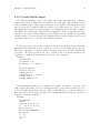
1
LSP User’s Manual and Reference
For LSP Version 8.7 (11 Aug 2005)
R. E. Clark and T. P. Hughes
Edited by Anat Sichel
c 1997-2005 Mission Research Corporation. This document describes the proCopyright °
cedures and parameters used for running the LSP code. It is written in Texinfo format,
which generates both a TeX file for printed output, and a GNU Info file for viewing on
a character-cell terminal. An HTML version is generated using the texi2html utility of
Lionel Cons (CERN). Texinfo and Info are distributed by the Free Software Foundation,
Inc.
Chapter 1: Introduction
1
1 Introduction
The LSP code package consists of the LSP simulation code, the GLSP graphical preprocessor, and the P4 graphical postprocessor. This section gives a brief description of each of
these codes, and references some third-party codes which can be used in conjunction with
LSP. The remainder of this document deals only with the LSP simulation code. The preand postprocessors have online documentation, and the third-party codes have their own
manuals.
1.1 LSP Simulation Code
LSP is a 3-D electromagnetic particle-in-cell (PIC) code designed for large scale plasma
simulations in either cartesian, cylindrical, or spherical coordinate systems. It can also be
used in 1-D and 2-D geometries. The code is designed to perform on parallel as well as serial
platforms. On parallel processors, domain decomposition with message-passing is used to
divide the computational load among the processors. A unified decomposition of fields and
particles is used; i.e., the particles reside on the same processor as the domain they occupy.
The standard message-passing interface (MPI) is used for inter-process communication.
The decomposition scheme is based on a two-level hierarchy. The problem space is
first divided into “regions” which are volumes that are conformal to the coordinate grid.
Each region is then divided into “domains” by one-dimensional slicing along any one of the
coordinate directions. The slicing direction can be different in each region. This method
is flexible enough to deal with complex geometries while at the same time minimizing the
number of processors needed at any given time. It has been found to be faster than a general
3-D decomposition. A queueing algorithm is used to manage inter-domain and inter-region
communication: processors send a signal to a designated region or global master processor
indicating the processors needed. The master processors maintain a queue of processes
which are ready and signal the process pairs to exchange relevant data.
LSP is written in C using an object-oriented style. Thus, there are “classes” for Grid,
Cell, Field, and Particle objects, consisting of data structures and “member functions”
which operate on the data. Message-passing and physics functions are kept separate. The
design allows new physics models to be added in a systematic manner.
Memory allocation for both fields and particles is fully dynamic. The code saves on
memory by not allocating field storage inside conducting surfaces. An array of pointers is
used to access data objects for each cell which contain all relevant field quantities. The
particles are managed in groups in linked lists for each species, and groups are added as
their population increases.
For electromagnetic simulations without particles, the code automatically skips both
the particle memory allocation and the particle-pushing algorithm. There is essentially no
run-time overhead associated with the presence of the particle-pushing code.
There are two electromagnetic field algorithms available: a standard (explicit) Yee
leapfrog algorithm, and an implicit algorithm. The implicit algorithm is particularly useful
in relaxing the courant limit on the timestep. An iterative electrostatic algorithm is also
available for situations in which fields are slowly varying. Grids can be specified in which the
spacing varies linearly in each coordinate; i.e., the cells can vary in size but the grid is still
2
LSP User’s Manual and Reference
R. E. Clark and T. P. Hughes
orthogonal. A first-order wave-absorbing boundary condition can be applied to openings
(ports) at any of the spatial boundaries.
There are several options for pushing particles. The standard momentum-conserving
PIC algorithm is the most widely known. This algorithm yields no self-particle forces but
is subject to the so-called Debye-length numerical instability that heats plasma electrons
until their Debye length reaches the grid cell size. An energy-conserving PIC algorithm is
also available that is not affected by the Debye length instability. A cloud-in-cell (CIC)
particle description is available that significantly reduces the noise level of the simulation
(see Section 4.4.21 [EXTENDED_PARTICLES], page 17). A direct implicit particle/field push
can be used in either the PIC or CIC models.
Algorithms are implemented for field emission, auxiliary circuit models, dielectrics, dispersive magnetic materials (RF absorption), secondary electron generation in materials,
multiple scattering and energy loss, surface heating and energy deposition, desorption of
neutrals from surfaces, ionization of neutrals, and interparticle collisions. A hybrid fluid
model has been implemented to work in concert with the collision algorithms. For all of the
above particle push options, a hybrid kinetic-fluid model can be invoked for any charged
particle species. The PIC or CIC method is used with either the usual kinetic equations
or a set of fluid equations in which the particle, in addition to the usual attributes, retains
an internal energy. A transition criteria is implemented that allows electron species to
transition back and forth from the two descriptions while conserving momentum exactly.
LSP particle and field data files are written in XDR format, allowing binary data to be
generated on a multiple-processor Unix computer and viewed on a different platform, e.g.,
a PC or Macintosh. The time history data file is an ASCII text file, and so is also portable.
Output can be examined using the P4 postprocessor (see Section 1.3 [P4 Postprocessor],
page 3), which is written in the IDL language (Research Systems Inc.).
The design of LSP was begun in June 1995 by Tom Hughes, Ren Yao and Bob Clark
under a DOE SBIR contract to investigate parallelization of particle methods.1 Currently,
LSP is maintained by Bob Clark, Tom Hughes, and Dale Welch. The code is licensed by
Mission Research Corporation, for commercial, GSA, and academic users.2
1.2 GLSP Preprocessor
GLSP is a point-and-click preprocessor for LSP. It functions as a tool to create a model
while enabling 3-D visualizatin of the spatial elements. Values can be entered as symbolic
expressions, allowing parametric specification of geometry, etc.
GLSP is the primary source of data entry and manipulation for LSP. An LSP simulation
can be, and generally is, launched from GLSP, or the input data created within GLSP can be
exported to a remote platform using an in-built FTP client. The P4 graphical postprocessor
can also be launched from GLSP. GLSP is written with C and Tcl/Tk and uses OpenGL
to render the objects in 3D space.
1
2
R. L. Yao, T. P. Hughes and R. E. Clark, “Parallelization of Smooth Particle Hydrodynamics on a
Distributed Memory Multiprocessor Computer”, MRC/ABQ-R-1763, Mission Research Corp., November
1995, SBIR Contract No. DE-FG03-923481298/II
LSP web site: ‘http://www.mrcabq.com’
Chapter 1: Introduction
3
Development of GLSP was started by Tom Hughes in 1997. Since 1999, Chris Mostrom
has been the primary developer. Development is ongoing and currently includes tutorials
(in the form of movies) to enhance ease of use. These tutorials include
beam_injection
rodpinch
rodpinch2
movie_making
1.3 P4 Postprocessor
P4 is a point-and-click postprocessor for LSP. It is used to view and print the History,
Particle, Vector, and Scalar dumps from LSP. It can also generate Particle and Scalar movies
in multiple formats, which can be viewed with other programs such as a Web browser or
Apple Quicktime. P4 is written in IDL and is cross-platform capable. It requires an IDL
runtime license.3
Development of P4 was started in 1996 by Tom Hughes, Bob Clark, and Ren Yao. Bob
Clark coded the first major release. Since 1999, Chris Mostrom has been the primary
developer, in collaboration with Bob Clark and Tom Hughes.
1.4 Integrated Tiger Series (ITS) Codes
The Monte Carlo treatment of electron transport in materials (see Section 6.9 [Medium
Models Input], page 73) uses the physics kernel of the Integrated Tiger Series (ITS) codes,
developed by John Halbleib and co-workers at Sandia National Laboratories and the National Institute of Standards and Technology.4 Using this part of LSP requires the XGEN
program which comes with the ITS 3.0 distribution. ITS can be licensed from the Radiation
Safety Information Computational Center at Oak Ridge National Laboratory.5
3
4
5
Research Systems Inc. web site: ‘http://www.rsinc.com/idl’
J. A. Halbleib, R. P. Kensek, G. D. Valdez, S. M. Seltzer, and M. J. Berger, “ITS: The Integrated TIGER
Series of electron/photon transport codes - version 3.0,” IEEE Trans. Nucl. Sci. NS-39, 1025 (1992).
RSICC web site: ‘http://epicws.epm.ornl.gov/rsic.html’
4
LSP User’s Manual and Reference
R. E. Clark and T. P. Hughes
Chapter 2: Conventions
5
2 Conventions
In this document, a vertical bar ‘|’ is used to indicate alternate values; e.g., X|Y|Z means
that the value X, Y, or Z can be used.
Coordinates are given in the order X, Y, Z and are separated by commas or blanks.
For 2-D simulations, only two coordinates are required and the unused direction need not
appear but may be entered for visual clarity. For 1-D simulations, only the x-coordinate
is used. In cylindrical geometry, these stand for (r, θ, z), and in spherical geometry they
represent (r, θ, φ). Optionally, the user may use ‘R’ in place of the symbol ‘X’ and ‘TH’ in
place of the symbol ‘Y’ when cylindrical or spherical geometry is being used, and ‘PHI’ in
place of ‘Z’ in spherical geometry.
The units for length are dependent upon which system of units has been specified by
the user (see Chapter 5 [User Units], page 25). The units for rotational coordinates in
cylindrical or spherical geometries are radians.
Input parameters for the simulation are governed through the input file. In this manual,
input file examples and references to input keywords and the values which follow them
appear in typewriter font. When the parameter values are alphanumeric symbols, they
can be written either in lowercase or uppercase characters, but the keywords (identifiers)
themselves are written only in lowercase. Values assigned to the parameters can be of four
types:
real:
Real numbers, e.g., 1.0, .01, -0.01, +1.0e-1
integer:
Integer numbers, e.g., 1, +1, -1
flag:
Can take the values ON (or, equivalently, TRUE), and OFF (or, equivalently,
FALSE)
string:
An alphanumeric string, without quotation marks, e.g., tantalum.tab
In the input examples, optional data are followed by an asterisk (*).
Keyboard input typed at command prompt is shown in this font.
The index also incorporates certain conventions. Concepts are shown in lower case.
Commands are shown in the same fonts as within the document. Each index entry is
followed by the section in which it is found.
We use the word “simulation” to refer to the entire process in the application of the LSP
code to some physical model, whereas the word “run” usually refers to a single period of
uninterupted calculation; that is, any simulation may require many runs, as determined by
time restraints or processor availability on the computer system being used.
6
LSP User’s Manual and Reference
R. E. Clark and T. P. Hughes
Chapter 3: Running LSP
7
3 Running LSP
LSP can be run on either single- or multiple-processor machines. The multiple-processor
version is initiated by using the MULTI_PROCESS compiler directive (see Section 4.4.41
[MULTI_PROCESS], page 20). An input file must be present in order for LSP to run (see
Chapter 6 [Input Variables], page 27) and a command file may be present (see Section 3.5
[Command File], page 11), but is optional.
3.1 Single-Processor Machines
The single-processor version of LSP will run on Unix, Windows, and Mac OS X workstations. At the command line or shell prompt, enter
lsp [-r] [-ra] [-n N] [-s] input.lsp
where ‘input.lsp’ is the user-supplied input file. To run in background with redirection of
terminal output, one can use ‘lsp [-opt] input.lsp >&log&’ (assuming a C shell), where
‘log’ is the name of the file containing the redirected output.
The optional ‘-r’ flag is used to restart a previous run from a restart dump, which
will have the name ‘restart.dat’ or ‘restart.alt’. This file is read after the input
file is processed. The restart file contains probe history, particle and field data from the
previous run. If the rename_restart_flag is ON (see Section 6.2.2.3 [rename_restart_
flag], page 32), then the most recent restart file may have the ‘.alt’ extension (this can be
determined by looking at the file dates). In this case, the file with the ‘.dat’ extension can
be removed from the simulation directory before restarting. The code will then attempt a
restart from the ‘.alt’ file. If this restart fails, the ‘.dat’ file can be used as a backup.
Alternatively, the ‘-ra’ option has the same effect as the ‘-r’ flag, except that the restart
is performed from the ‘restart.alt’ file instead of the ‘restart.dat’ file. This is a more
elegant way to restart from the ‘.alt’ file than moving or deleting the ‘.dat’ file.
Probe history data reside in the restart file and are written to the history file
‘history.p4’ when the restart run begins, so this file need not be preserved between
restarts. The user ordinarily increases one of the time_limit parameters on the input file
prior to restarting a simulation, unless the previous run was stopped before reaching this
limit. However, use of the number_of_steps parameter on a restart run will cause the
simulation to execute exactly that number of additional timesteps, unless the time_limit
is reached first.
The ‘-n N’ sequence, where N is an unsigned integer, will cause the code to run that
number of timesteps, regardless of what is specified on the input file. This may be useful
for checking the simulation setup without directly changing the input file.
The ‘-s’ option is used to perform initialization only and stops the run immediately
regardless of any time limits in the input file. This may also be useful for checking the
simulation setup before submitting a batch run, for example.
3.2 Multiple-Processor Machines
The multiple-processor version of LSP uses the MPI message-passing library
(‘http://www-unix.mcs.anl.gov/mpi/’). This version can make use of decomposition of
8
LSP User’s Manual and Reference
R. E. Clark and T. P. Hughes
the simulation space into separate domains in order to distribute the work-load among
multiple processes and thereby achieve faster running times.
The multiple-processor version of LSP produces a separate restart file for each region,
named ‘restart1.dat’, ‘restart2.dat’, . . . . All of these files must be present for the
restart to work correctly. If the rename_restart_flag is ON (see Section 6.2.2.3 [rename_
restart_flag], page 32), then the most recent restart files may have the ‘.alt’ extension
(this can be determined by looking at the file dates). In this case, the files with the ‘.dat’
extension can be moved out of the current run directory before restarting. The code will
then attempt a restart from the ‘.alt’ files. If this restart fails, the ‘.dat’ files can be used
as a backup by restoring them to the run directory. The most common reason for restart
failure is a corrupted or incomplete restart file due to time-limit termination while the file
was being written. A better way to restart a simulation from the ‘.alt’ files than moving
or deleting the ‘.dat’ files is to use the ‘-ra’ option on the command line instead of the
‘-r’ flag.
3.2.1 Workstation Network
On a workstation network with the MPICH version of MPI installed
(‘http://www-unix.mcs.anl.gov/mpi/mpich/’),
start a multiple-processor version of LSP using the p4 (no relation to the P4 postprocessor, Section 1.3 [P4
Postprocessor], page 3) communication device as follows:
lsp -p4pg pgroup [-opt] input.lsp
where the file ‘pgroup’ specifies a p4 processor group, such as
local 0
cerebro 1 /usr1/run7/lsp
achilles 1 /usr1/run7/lsp
which specifies that three processes are to be used (see Section 6.2.3.3 [number_of_
processes], page 33), one on the local computer, one on computer “cerebro” (which may
also be the local computer), and one on computer “achilles”. The path to the executable
on each computer must be supplied. The path also specifies the run directory, so the
executable, or a link to it, must be in the run directory.
3.2.2 DEC Cluster
On the DEC Unix cluster, start a multiple-processor version of LSP with:
dmpirun -np NP lsp [-opt] input.lsp
where ‘NP’ is the number of processes to use. This number must be the same as the number_
of_processes parameter in the input file (see Section 6.2 [Control Input], page 30).
3.2.3 Intel Teraflop
On the Intel Teraflop (ASCI Red), start LSP interactively on ‘NP’ processors using
yod -sz NP lsp [-opt] input.lsp >&log&
An NQS (Network Queueing System) job for ‘NP’ processors can be submitted to the
‘QUEUE’ queue on the Teraflop for a time ‘HH:MM:SS’ (hours:mins:secs) using
Chapter 3: Running LSP
9
qsub -q QUEUE -lP NP -lT HH:MM:SS -o log.lsp script.lsp
where ‘script.lsp’ is a shell-script file. An example of this file follows.
#!/bin/sh
date
cd $QSUB_WORKDIR
/cougar/bin/yod lsp [-opt] input.lsp
where QSUB_WORKDIR is a shell variable which resolves to the working directory from which
the qsub command is issued.
3.2.4 ASCIQ
On the ASCIQ system, start LSP interactively using
prun -n NP lsp [-opt] input.lsp >&log&
where ‘NP’ is the number of processors.
An LSF (Load Sharing Facility) job for ‘NP’ processors on ‘ND’ nodes can be submitted
to the ‘QUEUE’ queue on the ASCIQ for a time ‘MMM’ (min) using
bsub -q QUEUE -n NP -o log.lsp -W MMM prun -N ND lsp [-opt] input.lsp
Each node consists of 4 processors; therefore, a multiple of 4 must be used for ‘NP’ when
submitting a job beyond 4.
3.2.5 IBM-SP2
On the IBM-SP2, start LSP interactively using
lsp -procs NP [-opt] input.lsp >&log&
where ‘NP’ is the number of processors.
Generally, the IP switch will be used for interactive jobs. At the command prompt, type
setenv MP_EUILIB ip.
A LoadLeveler batch job can be submitted using
llsubmit script.lsp
where ‘script.lsp’ is a control file such as
#@ job_name
= run1
#@ initialdir
= /scratch2/mydir/
#@ notification
= always
#@ notify_user
= [email protected]
#@ error
= lsp.$(Cluster).err
#@ output
= lsp.$(Cluster).out
#@ job_type
= parallel
#@ requirements
= (Adapter == "hps_user")
#@ min_processors = NP
#@ max_processors = NP
#@ environment
= MP_EUILIB=us;MP_INFOLEVEL=3;MP_LABELIO=yes
#@ checkpoint
= no
#@ wall_clock_limit= HH:MM:SS
#@ account_no
= ACCOUNT_NUMBER
#@ queue
10
LSP User’s Manual and Reference
R. E. Clark and T. P. Hughes
set nodes = ‘echo $LOADL_PROCESSOR_LIST‘
cat ${nodes}
set runid = "run1"
cp -f $HOME/mydir/lsp .
cp -f $HOME/mydir/runs/${runid} .
lsp ${runid}
tar cvf ${runid}.tar ${runid} *.dat *.out *.err
compress -f ${runid}.tar
hpsscp ${runid}.tar.Z hpss:/s/hpss/myname/${runid}.tar.Z
echo "Job completed"
where ‘NP’ is the number of processors, ‘HH:MM:SS’ (hours:mins:secs) is the wall-time and
‘ACCOUNT_NUMBER’ is the user’s account.
3.3 Startup Messages
When LSP begins running, several lines of data relating to when and where it was
compiled, the compiler directives used, the input file name, and the start time are generated.
An example is:
Compiled Sat Nov 14 12:24:57 MST 1998 on achilles
Compiler flags: -O4 -std1 -warnprotos
Code options defined by user: -DSTATIC_FIELDS -DMULTI_PROCESS
Code options defined at compile-time:
STATIC_FIELDS
MULTI_PROCESS
Coordinate system used:
CARTESIAN
Input data file: input.lsp
Start time = Sat Nov 14 12:27:56 1998
The “code options” listed are those specified by the user at compilation time (see Chapter 4 [Compiling LSP], page 13). These options are also referred to as “compiler directives”.
3.4 Messages Generated By Errors in Input File
When starting an LSP run, a variety of error checking takes place to diagnose possible
mistakes in the choice of compiler directives and the specification of input data. These
errors will usually cause a printed message in standard output and prevent the simulation
from continuing. However, in some cases, a warning message may occur without stopping
the code from running. The user should be alert for this type of occurrence.
Chapter 3: Running LSP
11
3.4.1 Input Parameter Errors
Most of the data appearing in the input file for a simulation is syntax dependent. Interpretation by the LSP code is sensitive to the spelling and order of input parameters. At
present, the code issues an error message and exits immediately upon finding items in the
input text that cannot be identified.
3.4.2 Boundary Errors
The user is responsible for simulation set-up. However, LSP is able to check that at least
the boundaries of each domain (and therefore the entire simulation space) are well defined.
This means that some physical boundary condition is defined everywhere at the boundaries.
If any cells along an outer boundary are found not to be covered by one of the conditions
necessary for simulation fidelity, appropriate error messages are printed which locate the
portion of the grid containing the fault, and the simulation is aborted. An example is:
P0: boundary check error at ZMIN,
x-range 0.00e+00:1.00e+00, y-range 0.00e+00:0.00e+00
*** Error(s) on domain boundary detected ***
Domain boundary = ZMIN
Check input data for completeness
which indicates that the domain under control of process 0 has been found to have an
undefined boundary at the lower side in the z-coordinate. The most common cause for this
kind of error is a “hole” in the simulation boundary which can be patched with a conducting
surface.
3.5 Command File
While running a simulation, LSP checks periodically for a file named ‘command’ in the
directory from which it is started. This file may contain one of the following strings, which
cause the code to perform certain actions at the current timestep:
dump: Write all particle, scalar, field, and diagnostic dumps.
stop: Write a restart dump and stop the run.
abort: Stop the run with no restart dump.
rdump: Write a restart dump and continue.
report: Print domain statistics to gauge load balance.
particles: Print particle statistics by species.
balance: Rebalance the computational load among processes.
Under either Windows, Unix or Mac OS X, one can create the file ‘command’ containing
the word ‘stop’ with the command echo stop > command.
12
LSP User’s Manual and Reference
R. E. Clark and T. P. Hughes
Chapter 4: Compiling LSP
13
4 Compiling LSP
4.1 Compiling on Unix and Mac OS X
A makefile (called ‘Makefile’) is used to compile LSP. System-dependent parameters
and compiler directives are placed in a file ‘makedef’. ‘Makefile’ calls ‘madedef’. Sample
versions of ‘makedef’ currently exist for
• computers running Linux, with the MPICH version of MPI installed (‘makedef.linux)’
• computers running Mac OS X (10.2 or later recommended), with the MPICH version
of MPI installed (‘makedef.macosx’)
• DEC Alpha computer with the MPICH version of MPI installed (‘makedef.alpha’)
• DEC 8400 cluster (‘makedef.snl’)
• Intel TeraFlop at SNL (‘makedef.tflop’)
• ASCIQ system at LANL (requires MPI Default module) (‘makedef.asciq’)
To compile LSP on a particular computer, copy the appropriate file to ‘makedef’ (no
extension). Then edit ‘makedef’, inserting the desired compiler directives (see Section 4.4
[Compiler Directives], page 15) into the PFLAGS definition, e.g.:
# Preprocessor options:
PFLAGS = -DCYL_R_Z -DEXTERNAL_BFIELDS -DKELVIN_DEPOSITION -DMULTI_PROCESS
Now type make. Make calls ‘Makefile’. If compiler directives are changed, type make
new (which is equivalent to make clean followed by make).
‘Makefile’ may include commands to create documentation. These are referred to as
“targets”. These targets include
lsp.info:
Creates GNU Info files from the Texinfo file ‘lsp.txi’
lsp.html:
Creates HTML files from the Texinfo file ‘lsp.txi’
lsp.dvi:
Runs TeX on ‘lsp.txi’ to produce a DVI file ‘lsp.dvi’
lsp.ps:
Runs DVIPS on ‘lsp.dvi’ to produce a PostScript file ‘lsp.ps’
lsppdf.ps:
Runs DVIPS on ‘lsp.dvi’ to produce a PostScript file ‘lsppdf.ps’ suitable for
conversion to Adobe PDF format.
The target ‘alldocs’ creates all of the documentation formats listed above.
4.2 Compiling on MS Windows
LSP can be compiled with the Microsoft Visual C++ (“VC++”) compiler (Version 4 or
later). The first time an executable is created, the following steps are required.
1. Create a “Win32 Console Application” project and import the LSP sources.
2. Add the XDR library ‘xdr.lib’ to the project files.
14
LSP User’s Manual and Reference
R. E. Clark and T. P. Hughes
3. Add a path to an include directory containing the subdirectory ‘rpc’ where the
files ‘xdr.h’ and ‘types.h’ reside (e.g., Project-Settings-C/C++-PreprocessorAdditional include directories).
4. Ensure that the preprocessor definition WIN32 is defined (e.g., Project-SettingsC/C++-Preprocessor-Preprocessor definitions). The compiler directives (see Section 4.4 [Compiler Directives], page 15) may also be set here, or one can use the
‘lspmake’ script.
5. Add ‘wsock32.lib’ to the default libraries to link against (e.g., Project-SettingsLink-Object/library modules).
The files are ready to be compiled and linked. Once a makefile ‘lsp.mak’ has been
generated by VC++ (Project-Export Makefile), compiler directives can be input by either
using the Perl script ‘lspmake.bat’ or by typing them into the Project-Settings window.
The compiler directives are typed into the file ‘make.pc’ in the source directory, e.g.,
CYL_R_Z EXTERNAL_BFIELDS KELVIN_DEPOSITION MULTI_PROCESS
‘Make.pc’ is read by ‘lspmake.bat’.
If the compiler directives have been changed since the last compile, then type lspmake
[-d] clean, followed by lspmake [-d], in the source directory. Use the [-d] option for
the “Debug” instead of the “Release” version.
[(Note): The clean step is not needed unless compiler directives have changed. In
addition, if the VC++ environment variables have not been set at boot time, the file
‘VCVARS32.BAT’ (generated during installation of VC++) should be run before using
‘lspmake.bat’.]
4.3 Error Messages Generated by Incorrect Compilation
4.3.1 Data Type Errors
LSP requires the various data types in C to have specific sizes. Therefore, data types are
checked to ensure that the size specification is correct. Often, the problem is with the ‘long
int’ data type, which must be 8 bytes. On many systems, the data type having that size
is ‘long long int’. To accomplish this globally, the user must simply define the compiler
directive LONG_LONG_INT (see Section 4.4.34 [LONG_LONG_INT], page 19).
4.3.2 Unknown Compiler Directive Errors
Incorrect usage of compiler directives may cause an error message. This is usually the
result of misspelling one of the standard options in the list of compiler directives specified
by the user. An example is:
Compiled Tue Jan 22 10:30:16 MST 2002 on mrcdec.mrcabq.com
Compiler flags: -g -std1
Code options defined by user: -DCYL_R_Z -DCHARGE_DENISTY
Code options defined at compile-time:
Chapter 4: Compiling LSP
15
CYLINDRICAL
CYL_R_Z
*** Fatal error - Code compiled with unknown option: CHARGE_DENISTY
Simulation abort on Tue Jan 22 10:33:37 2002
Here the user specified CHARGE_DENISTY in the list of defined compiler options where
CHARGE_DENSITY was intended.
4.3.3 Incompatible Compiler Directive Errors
There are some combinations of compiler directives which are incompatible. In this case,
a compiler error message will appear and the compilation will stop. Some options require
another option to be included. Again, if not defined correctly, an error occurs causing the
compilation to stop.
4.4 Compiler Directives
4.4.1 CAR_ONE
Use 1-D cartesian (x) coordinates.
4.4.2 CAR_X_Y
Use 2-D cartesian (x-y) coordinates.
4.4.3 CAR_X_Z
Use 2-D cartesian (x-z) coordinates.
4.4.4 CARTESIAN
Use 3-D cartesian (x-y-z) coordinates. This is the default coordinate system.
4.4.5 CHARGE_DENSITY
Computes total charge density as a cell quantity. Required if the electrostatic field solver
is used (see Section 4.4.53 [STATIC_FIELDS], page 22), otherwise optional for diagnostic
purposes. Automatically defined if STATIC_FIELDS is defined.
4.4.6 CHARGE_DEPOSITION
Turns on charge deposition on material surfaces.
16
LSP User’s Manual and Reference
R. E. Clark and T. P. Hughes
4.4.7 COLLISIONAL_PLASMA
Enable particle interactions which occur in dense plasmas, such as ionization (see Section 6.17.10 [ionization], page 122) and scattering phenomena. The ionization model is applied every ionization_interval timesteps (see Section 6.2.7.1 [ionization_interval],
page 38). The scattering model is applied every scattering_interval timesteps (see Section 6.2.7.2 [scattering_interval], page 38).
4.4.8 CURRENT_CORRECTION
Turns on the current correction algorithm, for use with either the explicit or the implicit
electromagnetic field algorithms.
4.4.9 CURRENTS_OFF
Turns off effect of particle currents on the electromagnetic field solution (for debugging).
4.4.10 CYL_ONE
Use 1-D cylindrical (radial) coordinates.
4.4.11 CYL_R_TH
Use 2-D cylindrical (r-theta) coordinates.
4.4.12 CYL_R_Z
Use 2-D cylindrical (r-z) coordinates.
4.4.13 CYLINDRICAL
Use 3-D cylindrical (r-theta-z) coordinates.
4.4.14 DELAY_BREAKDOWN
Enable specification of a temporal dependence function for modification of emission
current after breakdown.
4.4.15 DESORPTION_ON
Enable use of the neutral desorption model.
4.4.16 DIRECT_IMPLICIT
Use the direct-implicit field and particle advance which is an implementation of the fully
damped D1 scheme (Ref.[2]). Note that DIRECT_IMPLICIT implies IMPLICIT_FIELDS, as
long as STATIC_FIELDS is not defined. See Section 4.4.30 [IMPLICIT_FIELDS], page 19.
Chapter 4: Compiling LSP
17
4.4.17 DOUBLE_PRECISION
Use double precision for all floating-point operations.
4.4.18 DYNAMIC_FIELDS
Solve the electromagnetic fields with one of the dynamic field solvers (explicit or implicit).
This option is the default and is necessary only if the fields are pre-calculated with a static
field solver prior to advancing the simulation electromagnetically. See Section 6.2.4.11
[field_initialization_flag], page 35.
4.4.19 ENERGY_DEPOSITION
Enables energy deposition on dense material surfaces or in a tenuous gas. This is used in
conjunction with certain medium models, specifically the method 1 model of either DENSE
or TENUOUS type, and the method 4 model of TENUOUS type only (see Section 6.9 [Medium
Models Input], page 73).
4.4.20 EXACT_IMPLICIT
Solve electromagnetic fields using the “unconditionally stable” ADI procedure as opposed
to the conventional ADI scheme, which is iterative in nature and not necessarily stable. This
directive can be used as a replacement for the IMPLICIT_FIELDS directive, which invokes
the conventional solution when used alone (see Section 4.4.30 [IMPLICIT_FIELDS], page 19).
4.4.21 EXTENDED_PARTICLES
Enables the extended particle CIC model in which the size of the particle “cloud” effectively covers two grid cells in each coordinate dimension instead of the usual one cell.
The resulting self-force of a particle is reduced by the corresponding reduction in particle
density (factor of 2 in 1-D, 4 in 2-D and 8 in 3-D). The key benefit of this treatment is
that numerical collisionality is greatly reduced while maintaining good energy conservation.
Note that, with the explicit particle-push option, good energy conservation is possible only
if the plasma skin depth is adequately resolved.
Warning - this compiler option may not work with complete fidelity under all circumstances. The case that should be avoided is when all of the following are used simultaneously:
1) 3-dimensions, 2) multiple regions, 3) explicit field solution, and 4) particle_forces_
option set to PRIMARY for any of the particle species defined in the simulation.
4.4.22 EXTERNAL_BFIELDS
Enables external magnetic fields to be defined by the user, either by functional prescription or from data files, and applied to particle forces. In addition, the definition must
be equal to the number of instances of those types of applications if more than one is required. Note that this directive is not required for simple constant values of applied field
(see Section 6.15 [External Fields Input], page 100).
18
LSP User’s Manual and Reference
R. E. Clark and T. P. Hughes
4.4.23 EXTERNAL_EFIELDS
Enables external electric fields to be defined by the user, either by functional prescription
or from data files, and applied to particle forces. In addition, the definition must be equal
to the number of instances of those types of applications if more than one is required. Note
that this directive is not required for simple constant values of applied field (see Section 6.15
[External Fields Input], page 100).
4.4.24 EXTRA_MOTION
Enables particles to travel more than one cell in a timestep. Usually, when the timestep
is limited by the Courant condition, this is not necessary. But in cases where this limitation
is not enforced, either by static field solution or by implicit field solution, this directive
should be used. One disadvantage of this directive is that at domain boundaries, particles
that move more than a single cell beyond that boundary in a timestep will be held back,
which may be undesirable. If so, the user may want to use the INTER_DOMAIN_TRACKING
directive, which may have slightly less running efficiency (see Section 4.4.31 [INTER_DOMAIN_
TRACKING], page 19).
4.4.25 FLUID_PHYSICS
Enables electrons or ions to be treated using fluid equations instead of kinetic equations
in a collisional plasma. This is used in conjuction with either the COLLISIONAL_PLASMA
or the SCATTERING_ON compiler directives. Fluid species are indicated by turning on the
fluid_species_flag in the [Particle Species] section of input (see Section 6.16 [Particle
Species Input], page 104).
4.4.26 FLUID_SPECIES=#
Sets the number of fluid species allowed in a simulation. Used in conjunction with the
FLUID_PHYSICS compiler directive (see Section 4.4.25 [FLUID_PHYSICS], page 18).
Default: 1
4.4.27 FREESPACE_PML
Enables the modeling of freespace with one of the perfectly matched layer (PML) techniques. The two available models are the so-called uniaxial PML, also known as the unsplit
version, and the convolutional PML, also known as the complex frequency shifted PML
(CFSPML) in its most generalized form. The user must invoke this directive in order to
use the PML options under the freespace boundary model (see Section 6.6.4 [Freespace
Boundaries], page 69).
4.4.28 FRICTIONAL_EFFECTS
Enables frictional (drag) effects between species in a collisional plasma. This is used in
conjuction with either the COLLISIONAL_PLASMA or the SCATTERING_ON compiler directives.
However, frictional effects can only be used when the direct-implicit algorithm has been
invoked (see Section 4.4.16 [DIRECT_IMPLICIT], page 16).
Chapter 4: Compiling LSP
19
4.4.29 FULL_SUSCEPTIBILITY
Uses the full complement of off-diagonal terms of susceptibility for calculating correction currents. Susceptibility is a property of the direct-implicit algorithm (see Section 4.4.16
[DIRECT_IMPLICIT], page 16). These additional terms are ordinarily used in the conventional iterative ADI field solution, but not in the “unconditionally stable” version (see
Section 4.4.20 [EXACT_IMPLICIT], page 17). This directive should be used with caution it provides a first-order correction only, and is not accurate when fields are changing too
rapidly, for example. In such cases it would be advisable to use the iterative ADI solution
instead.
4.4.30 IMPLICIT_FIELDS
Uses the ADI field solver. With this option, only fields are treated implicitly. Particles
are not. In order to treat particles implicitly, the DIRECT_IMPLICIT option must be defined
(see Section 4.4.16 [DIRECT_IMPLICIT], page 16).
4.4.31 INTER_DOMAIN_TRACKING
Enables particles to travel more than one cell in a timestep, even across domain boundaries. This can be used in place of the EXTRA_MOTION compiler directive (see Section 4.4.24
[EXTRA_MOTION], page 18). The difference between them is that EXTRA_MOTION used alone
will hold back particles which, during a timestep, move more than a single cell after crossing a domain boundary, whereas using INTER_DOMAIN_TRACKING will result in unaltered
trajectories at a slight expense in running efficiency.
4.4.32 IONIZATION_ON
Enables the ionization model, which is a subset of the collisional plasma model (see
Section 4.4.7 [COLLISIONAL_PLASMA], page 16). Whenever this directive is used, the compiler
directive MUTABLE_SPECIES must also be defined (see Section 4.4.42 [MUTABLE_SPECIES],
page 20).
4.4.33 KELVIN_DEPOSITION
Turns on thermal surface heating in material structures, provided that one of the appropriate medium models is specified for them. This applies to the method 1, method 3,
and method 4 medium models (see Section 6.9 [Medium Models Input], page 73). This
thermal deposition can be used for diagnostic purposes, but it is necessary for any particle
emission model in which a thermal breakdown is in effect (see Section 6.17.2.3 [threshold
(emission)], page 113).
4.4.34 LONG_LONG_INT
Defines long long int instead of long int data type for compilers that require that
extension in order to get an 8-byte integer.
20
LSP User’s Manual and Reference
R. E. Clark and T. P. Hughes
4.4.35 MAGNETIC_DISPERSION
Required if the ferrite (complex magnetic permeability) model is to be used (see Section 6.11.4 [ferrite], page 94).
4.4.36 MAGNETIC_HYSTERESIS
Required if the magnetic hysteresis model is to be used (see Section 6.11.5 [hysteresis],
page 95).
4.4.37 MAGNETOSTATIC
Solve for magnetostatic fields. This is used in conjunction with the STATIC_FIELDS
option (see Section 4.4.53 [STATIC_FIELDS], page 22).
4.4.38 MAGNETOSTATIC_FFT2D
Solve for transverse magnetostatic fields using the FFT method, assuming rectangular
conducting simulation boundaries. Useful for some paraxial beam simulations.
4.4.39 MAX_RESONANCES=#
Sets the maximum number of resonant frequencies in the ferrite model (see Section 6.11.4
[ferrite], page 94).
4.4.40 MAX_SPECIES=#
Sets the maximum number of particle species present in the simulation for the particle
scattering model (see Section 4.4.48 [SCATTERING_ON], page 21). Also used whenever particle
densities by species are required (see Section 4.4.44 [NUMBER_DENSITIES], page 21). The
default value is 1, but must be set to a larger value when the number of species entered on
input is more than one.
Default: 1
4.4.41 MULTI_PROCESS
Enables the use of multiple processes to sub-divide a simulation into domains.
4.4.42 MUTABLE_SPECIES=#
Defines the maximum number of “mutable” species present in the simulation, that is,
those that can be ionized to a higher charge state. This directive is used in conjunction
with the IONIZATION_ON compiler directive (see Section 4.4.32 [IONIZATION_ON], page 19)
for the ionization model (see Section 6.17.10 [ionization], page 122). To set this properly,
count the number of species in the [Particle Species] section which can be ionized to a
higher charge state: the value of MUTABLE_SPECIES should be greater than or equal to this
number (see Section 6.16 [Particle Species Input], page 104).
Default: 1
Chapter 4: Compiling LSP
21
4.4.43 NO_PARTICLES
Eliminates particle-related code from compilation. The advantage of this option is that
a smaller executable file can be used for simulations which require no particles.
4.4.44 NUMBER_DENSITIES
Includes number densities for each particle species as cell quantities. This is required
for the ion-ion stripping model (see Section 6.17.11 [higherstate], page 123), or may be
used simply for diagnostic purposes. Whenever this directive is used, the compiler directive
MAX_SPECIES must also be defined (see Section 4.4.40 [MAX_SPECIES], page 20).
4.4.45 PARTICLE_COLLAPSE
Allows use of the particle collapse algorithm, which vastly reduces the number of particles
present by combining pairs of particles in the same cell and with similar velocities (see
Section 6.18 [Particle Collapse Input], page 134).
4.4.46 PRIMARY_SPECIES=#
Sets the species number to be used as the primary species for the simulation. For
example, the method 2 scattering medium model (see Section 6.9.32 [method 2], page 81) is
applied only to the primary species and no other.
Default: 1
4.4.47 QUASINEUTRAL_FIELDS
Solve the EM-fields by the quasi-neutral Darwin approximation, that is, with displacement current neglected. This involves modification of the usual Maxwell equations in which
Ohm’s Law is used instead of Ampere’s Law, while still retaining Faraday’s Law.
4.4.48 SCATTERING_ON
Enables the scattering model, which is a subset of the collisional plasma model (see
Section 4.4.7 [COLLISIONAL_PLASMA], page 16). Whenever this directive is used, the compiler
directive MAX_SPECIES must also be defined (see Section 4.4.40 [MAX_SPECIES], page 20).
4.4.49 SPATIAL_FILTER
Invoke the use of diffusive terms to damp light waves spatially in the explicit electromagnetic field equations. See Section 6.2.4.9 [electric_spatial_filtering_parameter],
page 35, and Section 6.2.4.14 [magnetic_spatial_filtering_parameter], page 36.
4.4.50 SPH_ONE
Use 1-D spherical (radial) coordinates.
4.4.51 SPH_R_TH
Use 2-D spherical (r-theta) coordinates.
22
LSP User’s Manual and Reference
R. E. Clark and T. P. Hughes
4.4.52 SPHERICAL
Use 3-D spherical (r-theta-phi) coordinates.
4.4.53 STATIC_FIELDS
Solve the static field equations instead of electromagnetic equations. This directive
implies CHARGE_DENSITY as well (see Section 4.4.5 [CHARGE_DENSITY], page 15).
4.4.54 STATIC_FIELDS_FFT2D
Solve for transverse electrostatic fields using the FFT method, assuming rectangular
conducting simulation boundaries. Useful for some paraxial beam simulations.
4.4.55 STIMULUS_DEPOSITION
Use specific stimulating species for stimulated emission instead of the total charge deposition of all species at the emission surfaces. If more than one stimulating species is
required for different instances of the stimulated emission model, the STIMULUS_SPECIES
compiler directive must be set to that number (see Section 4.4.56 [STIMULUS_SPECIES],
page 22). Each stimulating species can only be used for a single stimulated model. See also
Section 6.17.5 [emission (stimulated)], page 114.
4.4.56 STIMULUS_SPECIES=#
When stimulated emission requires a specific stimulating species rather than the total
charge deposition, STIMULUS_SPECIES should be set to the total number of distinct stimulating species appearing in all stimulated emission input requests (see Section 6.17.5 [emission
(stimulated)], page 114).
Default: 1
4.4.57 SUBCYCLING_ON
Enable subcycling in the particle advancement whenever the cyclotron frequency becomes high enough to cause inaccuracy in the kinematical calculations.
4.4.58 TEMPORAL_FILTER
Use temporal filtering in the electromagnetic field equations. This is only appropriate
under certain conditions. For example, it is never used with any static-fields solution. It
can be used with the explicit-fields solution only if time-biasing is not being used. It can
also be used with the “exact” version of the implicit-fields solution. See Section 6.2.4.18
[temporal_filtering_parameter], page 36.
4.4.59 UNITS_CGS
User units are the standard cgs system of units.
Chapter 4: Compiling LSP
23
4.4.60 UNITS_MKS
User units are the standard mks system of units.
4.4.61 USE_CONDUCTIVITY
Include conductivities as a cell quantity. This directive is relevant to any of the dynamic
field soutions.
4.4.62 USE_OHMIC_TERMS
Include certain fluid-related properties of a plasma such as conductivity and fluid velocity
in the cells. These quantities are required for the conductivity model of a gaseous medium
(see Section 6.9 [Medium Models Input], page 73). It is invalid to use this directive with
any of the static field solutions (see Section 4.4.53 [STATIC_FIELDS], page 22).
4.4.63 USE_PERMEABILITY
Include the magnetic permeability, mu, as a cell quantity. This provides greater flexibility
in shaping paramagnetic materials using the medium models (see Section 6.9 [Medium
Models Input], page 73). This directive is required when using paramagnetic materials in
the ADI field solver (see Section 4.4.30 [IMPLICIT_FIELDS], page 19). It is invalid to use
this directive with any of the static field solutions (see Section 4.4.53 [STATIC_FIELDS],
page 22).
4.4.64 USE_PERMITTIVITY
Include the electric permittivity, epsilon, as a cell quantity. This provides greater flexibility in shaping dielectric materials using the medium models (see Section 6.9 [Medium
Models Input], page 73). This directive is required when using dielectric materials in the
ADI field solver (see Section 4.4.30 [IMPLICIT_FIELDS], page 19).
4.4.65 USE_PYTHON
Enable use of user-defined functions in Python format in the [Functions] section of
input (see Section 6.24 [Functions Input], page 144).
4.4.66 USE_SUBCELLS
Include the subcell structure as a cell quantity. This enables the use of subgrid modeling,
such as the 2-d slope model (see Section 6.13 [Subgrid Models Input], page 98).
4.4.67 USE_SUBSTRATE
Enable use of the substrate model, which may be restricted by export control (see Section 6.14 [Substrate Models Input], page 99).
4.4.68 USE_QEOS
Enable use of the qeos model, which may be restricted by export control.
24
LSP User’s Manual and Reference
R. E. Clark and T. P. Hughes
4.4.69 USE_XSEC
Enable use of the ITS (method 4) medium model (see Section 6.9.34 [method 4], page 83),
which may not be available in all releases of the LSP code. It is restricted to users who
have an ITS licence.
4.4.70 VOLUME_WEIGHTING
Use volume weighting, rather than linear, for particle contributions to charge densities
and currents when a cylindrical coordinate system is being used.
Chapter 5: User Units
25
5 User Units
The system of units used for input and output values can be set at compile time to one
of three different conventions. See Section 4.4 [Compiler Directives], page 15. Two of them
are the standard mks and cgs (SI) units. The third one offered is the native “LSP user
units,” which is the default condition. The latter has been found to be very practical for
running simulations. All physical quantities mentioned in this manual are in user units,
unless otherwise specified.
5.1 LSP Units
mass ........................................................gram
time ..................................................nanosecond
length ................................................centimeter
charge ..............................................microcoulomb
current ...................................................ampere
potential ...............................................kilovolt
electric field ...................................kilovolt per cm
magnetic field .............................................gauss
field energy ...............................................joule
particle energy ....................................electron volt
temperature ...............................................kelvin
resistance ...................................................ohm
capacitance ............................................nanofarad
inductance .............................................nanohenry
conductivity ......................................inverse second
5.2 MKS Units
mass ....................................................kilogram
time ......................................................second
length .....................................................meter
charge ...................................................coulomb
current ...................................................ampere
potential ...................................................volt
electric field ....................................volt per meter
magnetic field .............................................tesla
field energy ...............................................joule
particle energy ....................................electron volt
temperature ...............................................kelvin
resistance ...................................................ohm
capacitance ................................................farad
inductance .................................................henry
conductivity ...................................inverse ohm-meter
5.3 CGS Units
mass ........................................................gram
time ......................................................second
26
LSP User’s Manual and Reference
R. E. Clark and T. P. Hughes
length ................................................centimeter
charge ...............................................statcoulomb
current ...............................................statampere
potential ...............................................statvolt
electric field ...................................statvolt per cm
magnetic field .............................................gauss
field energy .................................................erg
particle energy ....................................electron volt
temperature ...............................................kelvin
resistance .........................................second per cm
capacitance ...........................................centimeter
inductance ..................................square second per cm
conductivity ......................................inverse second
Chapter 6: Input Variables
27
6 Input Variables
The input file is divided up into a number of sections dealing with various aspects of
simulation design. Each section consists of a section header, contained in square brackets,
followed by the input parameters belonging to that section. Sections are not required unless
so noted.
[Title]
Simulation title which, when specified, overrides the default code-generated title
[Control]
Timestep, time limit, algorithmic and diagnostic parameters (required)
[Grid]
Defines overall simulation grid coordinates and spacing (required)
[Regions]
Specifies zones into which the simulation space is broken up
[Objects]
Geometrically shaped objects which describe the simulation structure
[Boundaries]
Boundary conditions on the simulation other than conducting boundaries,
which are specified in the [Objects] section
[Potentials]
Iteration parameters and boundary values for the electrostatic field solver
[Materials]
Allows for user specified materials beyond those which are available internally
[Medium Models]
Specifies material properties associated with structural objects defined in the
[Objects] section
[Circuit Models]
Circuit models used as adjuncts to the simulation grid
[Volume Models]
Grid-conformal rectangular regions of dielectrics, magnetic materials, current
drive, etc.
[Liner Models]
Parameters for a simple imploding liner
[Subgrid Models]
Specifies parameters for the so-called subgrid models, such as a smooth slope
[Substrate Models]
Neutral ion source model for a metallic plate embedded in a ceramic material
[External Fields]
Specifies externally applied electric and/or magnetic fields
[Particle Species]
Specifies parameters such as charge, mass, etc. for each particle species present
(required for particles)
28
LSP User’s Manual and Reference
R. E. Clark and T. P. Hughes
[Particle Creation]
Particle generation models: injection, emission, etc. (required for particles)
[Particle Collapse]
Control parameters for reduction of particle number by coalescence of macroparticles
[Particle Migration]
Control parameters for electron migration between kinetic and fluid states
[Particle Extraction]
Used to generate data files of particles crossing specified planes, e.g., for subsequent use in a slice transport code or as input to LSP using the fileread
option
[Particle Interaction]
Controls interactions between particle species for ionization and scattering models
[Particle Diagnostics]
Used to generate data files containing particle diagnostic measurements as functions of some specified variable
[Particle Targets]
Used to generate 2-D diagnostic maps of cumulative fluence, energy, and divergence of particles passing through target planes
[Functions]
Specifies tabulated or analytic functions to be used during the simulation
[Probes]
Time-sampled diagnostics for field and particle measurements
Descriptions for the parameters for each of these sections follow. Except for the
[Control] section, the parameters must appear in the same order as that given in the
examples. Also, except for the [Control] section, all parameters must appear, except those
designated with an asterisk (*) in the input examples, which are optional. The sections
themselves may appear in any order in the input file.
A good way to set up a simulation is to copy and edit the examples from this manual.
Note that, while the keywords themselves must appear with the exact spelling indicated,
their values, when alphanumeric, may appear as lowercase or uppercase or even mixed.
The spelling of section headers must be exactly the same as shown: with individual words
beginning in uppercase letters.
Blank lines and lines beginning with a semicolon ‘;’ in the input file are ignored. A
semicolon may be placed anywhere on a line to insert a comment. Everything after the
semicolon on the line is ignored.
The order in which the input sections appear below is one possible order in which they
might appear in an input file.
Chapter 6: Input Variables
29
6.1 Title Input
The [Title] section of the input file specifies a title to be used in all output files for
identification of the simulation. If not specified, the default generic title used is: “LSP
simulation”. The input file name and the time-stamp generated at the beginning of the
simulation run are appended to the title. The simulation title must be contained within
double quotes.
An example is:
[Title]
simulation_title "This is a title"
30
LSP User’s Manual and Reference
R. E. Clark and T. P. Hughes
6.2 Control Input
The [Control] section of the input file specifies the timestep, simulation time, algorithmic and diagnostic parameters, etc. In this section (and only this one), the parameters
may be specified in any order. All of these parameters are optional and are not required to
run a simulation. However, without some minimal parameters, such as a time limit and a
timestep specification, nothing meaningful would be calculated. There are many parameters
from which to select. The parameters are listed alphabetically and discussed individually
below.
An example is:
[Control]
courant_multiplier 0.9
time_limit_ns 20.0
time_bias_coefficient 0.5
time_bias_iterations 4
probe_interval 5
dump_interval_ns 10.0
particle_movie_interval 100
restart_interval_ns 10.0
number_of_processes 8
balance_interval_ns 1.0
load_balance_flag ON
region_balance_flag OFF
report_timing_flag ON
rename_restart_flag ON
6.2.1 Temporal Parameters
6.2.1.1 courant multiplier (real)
Any positive value of courant_multiplier will cause the code to determine the simulation timestep by searching the grid for the smallest Courant-limited timestep, assuming
cartesian coordinates, and multiplying it by the value of the courant_multiplier. In cylindrical coordinates (see Section 4.4.13 [CYLINDRICAL], page 16), a value of about 0.9 or less is
required for stability. In cartesian coordinates, a value of 1 can be used. The input value for
the time_step parameter (see Section 6.2.1.4 [time_step], page 31) will take precedence if
it is smaller than the internally calculated value.
6.2.1.2 number of steps (integer)
Number of timesteps for a simulation run. This parameter takes precedence over time_
limit if it is reached first. If it is used in a restart operation, the simulation will execute
that number of timesteps more from the previous run unless the time_limit parameter is
reached first. In other words, on restarts, it is not the cumulative timestep count for the
simulation, but simply the number of timesteps executed for that run.
Chapter 6: Input Variables
31
6.2.1.3 time limit (real)
Options for this parameter are:
time_limit:
Total physical time in user units to run the simulation; that is, the time at
which the simulation stops running.
time_limit_ns:
Total physical time in ns to run the simulation.
time_limit_cm:
Total physical time to run the simulation in units of 1 cm/c, where c is the
velocity of light. Since relativistic electrons travel at about c, this is sometimes
a convenient way of specifying the simulation time.
The value of number_of_steps, if it is reached first, takes precedence over time_limit.
6.2.1.4 time step (real)
Options for this parameter are:
time_step:
Physical timestep in user units.
time_step_ns:
Physical timestep in ns.
time_step_cm:
Physical timestep in units of 1 cm/c, where c is the velocity of light. Since
relativistic electrons travel at about c, this is sometimes a convenient way of
specifying the timestep.
6.2.2 Simulation Restarts
6.2.2.1 dump restart flag (flag)
If dump_restart_flag is ON, automatically dump the restart file(s) at the end of the
simulation, that is, at termination time (see Section 6.2.1.3 [time_limit], page 31).
Default: OFF
6.2.2.2 maximum restart dump time (real)
Maximum wall-clock time between restart dumps in hours.
Default: 1.e9 hours (i.e., infinite)
32
LSP User’s Manual and Reference
R. E. Clark and T. P. Hughes
6.2.2.3 rename restart flag (flag)
If rename_restart_flag is ON, alternate the filename extension on successive restart
dumps between .dat and .alt. This is a safety measure in case the run is interrupted
unintentionally during the output of the restart dump. An uncorrupted restart dump will
remain with only the amount of calculation between those two restart dumps having been
lost.
Default: OFF
6.2.2.4 restart interval (real)
Options for this parameter are:
restart_interval:
Number of timesteps between restart dumps.
restart_interval_time:
Interval in user units between restart dumps.
restart_interval_ns:
Interval in ns between restart dumps.
restart_interval_cm:
Interval in units of 1 cm/c, where c is the velocity of light between restart
dumps.
Default: 1.e+9 (no dumps)
6.2.3 Parallel Processing
6.2.3.1 balance interval (real)
When running on a multiple-processor computer, LSP can move domain boundaries to
rebalance the computational load among the processors. This parameter sets the interval
at which the code checks to see if load balancing is needed. (see Section 6.2.3.2 [load_
balance_flag], page 33 and Section 6.2.3.4 [region_balance_flag], page 33.)
Options for this parameter are:
balance_interval:
Number of timesteps between load-balance checks.
balance_interval_time:
Interval in user units between load-balance checks.
balance_interval_ns:
Interval in ns between load-balance checks.
balance_interval_cm:
Interval in units of 1 cm/c, where c is the velocity of light between load-balance
checks.
Default: 1.e+9 (no rebalances)
Chapter 6: Input Variables
33
6.2.3.2 load balance flag (flag)
If load_balance_flag is ON, check the load balance between processes every balance_
interval intervals (see Section 6.2.3.1 [balance_interval], page 32). The rebalance procedure, if needed, is performed only within regions, rather than between regions (see Section 6.2.3.4 [region_balance_flag], page 33).
Default: ON
6.2.3.3 number of processes (integer)
Number of processes to be used for the simulation. On a multiple-processor computer,
each process is typically started on a different processor, if available. The number must be
equal to the total number of domains into which the simulation space has been divided.
6.2.3.4 region balance flag (flag)
If region_balance_flag is ON, perform load balancing across regions as well as within
regions. This enables processes to migrate between regions. The load_balance_flag must
also be ON for this option.
Default: OFF
6.2.3.5 initial balance flag (flag)
If initial_balance_flag is ON, perform load balancing shortly after run initialization,
either at t=0, or when restarting a simulation. This is useful in the latter case when changing
the number of processes to be used, or when the override_balance_flag is set to ON, that
is, whenever the simulation may not be in a balanced state. The load_balance_flag must
also be ON for this option.
Default: OFF
6.2.3.6 override balance flag (flag)
The override_balance_flag only effects restart runs from previously generated restart
dumps in which load-balancing has occurred. If override_balance_flag is ON, any loadbalancing information on the restart file is ignored, and the simulation is continued in
the domain configuration specified on the input file. If the load_balance_flag is left ON,
however, load-balancing will continue at the next opportunity.
Default: OFF
6.2.3.7 load timing interval (integer)
Information on the CPU time taken for the field solution and the particle algorithm are
accumulated over this interval prior to the load-balance evaluation, which depends on these
data.
Default: 1
6.2.4 Field Solution and Modification
34
LSP User’s Manual and Reference
R. E. Clark and T. P. Hughes
6.2.4.1 applied current (real)
The value for the applied_current parameter is used to initialize the Y- or Thetacomponent of magnetic fields in the simulation space. The primary use of this parameter is in conjunction with the hysteresis volume model to start the simulation with B
and H fields at some values on the lower end of the hysteresis curve (see Section 6.11.5
[hysteresis], page 95).
Default: 0.0
6.2.4.2 background electron conductivity (real)
This parameter is used in the quasi-neutral field solution to set the value of the total background conductivity which is applied to electron currents. (see Section 4.4.47
[QUASINEUTRAL_FIELDS], page 21).
Default: 1.e13 in inverse seconds
6.2.4.3 background plasma density (real)
This parameter is used in the quasi-neutral field solution to set the value of the electron
density in the background plasma. (see Section 4.4.47 [QUASINEUTRAL_FIELDS], page 21).
Default: 1.e10 in number/cubic-centimeter
6.2.4.4 cold test flag (flag)
If cold_test_flag is ON, run the simulation without particles. Any particle-creation
statements in the input file are ignored.
Default: OFF
6.2.4.5 convergence iterations (integer)
Maximum number of iterations to be used in any of the various iterative field solutions.
Fewer iterations are used when the solution satisfies the convergence criterion. A warning
message is usually printed if this limit is reached without convergence. This parameter can
be used instead of implicit_iterations or potential_iterations.
6.2.4.6 convergence tolerance (real)
Convergence criterion for any of the various iterative field solutions. Values typically
range from 1.e-3 to 1.e-7, possibly smaller, depending on the type of field solution being used.
This parameter can be used instead of implicit_tolerance or potential_tolerance.
Default: 1.e-3
6.2.4.7 dielectric kill flag (flag)
If dielectric_kill_flag is ON, kill any particles that impact a dielectric material,
whether it is a volume model (see Section 6.11 [Volume Models Input], page 92) or a
medium model of method 0 (see Section 6.9 [Medium Models Input], page 73).
Default: ON
Chapter 6: Input Variables
35
6.2.4.8 electric force filtering parameter (real)
Applies temporal smoothing to the electric field applied to particles. The value, in the
range 0–1, multiplies the old electric field. This parameter should not be used with implicit
particles, that is, when the DIRECT_IMPLICIT compiler option is defined (see Section 4.4.16
[DIRECT_IMPLICIT], page 16).
Default: 0.0 (no filtering)
6.2.4.9 electric spatial filtering parameter (real)
Diffusion coefficient for spatial damping applied to electric field advance in the explicit
field solver (Ref.[1]). Typical values are in the range 0.1 to 0.25.
Default: 0.0 (no filtering)
6.2.4.10 field advance flag (flag)
If field_advance_flag is OFF, run the simulation without advancing the fields. Particles
are created and advanced in whatever fields exist when the simulation starts.
Default: ON
6.2.4.11 field initialization flag (flag)
If field_initialization_flag is ON, initialize the fields with one of the static solutions prior to temporal advancement with a dynamic field solver. This can be useful for
some simulations such as pre-setting a potential across charged plates and then proceeding
from that point with a fully electromagnetic field solution. Use of this option is the only
instance where both the STATIC_FIELDS and DYNAMIC_FIELDS compiler options are used
concurrently (see Section 4.4.53 [STATIC_FIELDS], page 22 and see Section 4.4.18 [DYNAMIC_
FIELDS], page 17).
Default: OFF
6.2.4.12 ion conductivity factor (real)
This parameter is used in the quasi-neutral field solution to set the value of the conductivity which is applied to ion currents. This simply multiplies the value of the electron
conductivity, which is determined by the background_electron_conductivity parameter
above. Value should never be zero. (see Section 4.4.47 [QUASINEUTRAL_FIELDS], page 21).
Default: 1.0
6.2.4.13 magnetic force filtering parameter (real)
Applies temporal smoothing to the magnetic field applied to particles. The value, in the
range 0–1, multiplies the old magnetic field. This parameter should not be used with implicit
particles, that is, when the DIRECT_IMPLICIT compiler option is defined (see Section 4.4.16
[DIRECT_IMPLICIT], page 16).
Default: 0.0 (no filtering)
36
LSP User’s Manual and Reference
R. E. Clark and T. P. Hughes
6.2.4.14 magnetic spatial filtering parameter (real)
Diffusion coefficient for spatial damping applied to magnetic field advance in the explicit
field solver. Typical values are in the range 0.1 to 0.25.
Default: 0.0 (no filtering)
6.2.4.15 small radius exclusion (real)
Used in 3-D cylindrical coordinates, to avoid the Courant instability limit on the timestep
due to small grid-spacing in the θ (Y) coordinate near the axis. THETA dependence is dropped
from the field equations inside a radius defined by the small_radius_exclusion value.
Should be used with caution.
6.2.4.16 time bias coefficient (real)
Backward-bias coefficient (0 ≤ α1 ≤ 1) in time-biased field solver:
E N − E N −1
= α1 ∇ × B N +1/2 + α2 ∇ × B N −1/2 − J N −1/2
∆t
B N +1/2 − B N −1/2
= −∇ × E N
∆t
where α1 + α2 = 1. A time_bias_coefficient value of 0 gives the unbiased (explicit)
algorithm. Biasing causes the electromagnetic fields to damp at a rate which increases with
wavenumber. It can be useful in damping numerical noise and instabilities (see Ref.[4]).
The implicit equations are solved iteratively.
6.2.4.17 time bias iterations (integer)
Number of iterations to be used in time-bias algorithm. Usually, the number of iterations
needs to increase with the value of time_bias_coefficient. Commonly used values are:
time_bias_coefficient
time_bias_iterations
0.125
2-3
0.25
3-4
0.5
4-6
0.75
6-16
More iterations cause the field-solver to run slower.
6.2.4.18 temporal filtering parameter (real)
Damping parameter in temporal filtering algorithm to suppress short-wavelength electromagnetic fields (see Ref.[9]). Requires the TEMPORAL_FILTER compiler directive (see
Section 4.4.58 [TEMPORAL_FILTER], page 22). A value of 0 recovers the undamped leapfrog
algorithm. This filtering is only appropriate in certain simulation conditions. For example,
it is never used with any static-fields solution. It can be used with the explicit-fields solution
only if time-biasing is not being used. It can also be used with the “exact” version of the
implicit-fields solution.
Default: 0.0 (no filtering)
Chapter 6: Input Variables
37
6.2.5 Implicit Field Algorithm
6.2.5.1 error current filtering parameter (real)
Applies temporal smoothing of the error currents in the direct-implicit method. The
range of this parameter is 0 to 1. Higher values give more smoothing and are generally
recommended for higher density plasmas.
Default: 0.0 (no smoothing)
6.2.5.2 implicit acceleration parameter (real)
Initial acceleration factor for the ADI field solution. The code will adjust this parameter,
if necessary, to help convergence.
Default: 0.0
6.2.5.3 implicit iterations (integer)
Maximum number of iterations to be used in the ADI method of advancing fields.
Requires either the IMPLICIT_FIELDS or the DIRECT_IMPLICIT compiler directive. The
ADI field solver is used with the direct-implicit particle push (Ref.[2]). See Section 4.4.16
[DIRECT_IMPLICIT], page 16. Fewer iterations will be used if convergence is reached. A
warning message is printed if this limit is reached without convergence. Also, a printout
of the number of iterations used can be obtained using the print_convergence_flag, or
the iteration count can be put onto the time history file by requesting a convergence
iterations probe (see Section 6.25.8 [Convergence Probes], page 154). Iteration numbers
greater than 10 usually indicate a problem with convergence. In this case, reducing the
simulation timestep is recommended.
6.2.5.4 implicit omega min factor (real)
An adjustment parameter for the minimum value of omega (acceleration parameter) used
in the ADI static field solution. The method is designed to cycle through values of omega
which cover the theoretical range of eigenvalues associated with the discretization of the
problem space. However, it has been found that this process can be optimized somewhat by
raising the minimum value slightly, thereby narrowing the entire range of omegas used. This
is done by specifying an adjustment parameter less than 1.0 and can only be determined
by trial-and-error. A representative number found in an early investigation was 0.25.
Default: 1.0
6.2.5.5 implicit subcycles (integer)
Number of subcycles to be used in the ADI method of the static field solution. Requires
either the IMPLICIT_FIELDS or the DIRECT_IMPLICIT and the STATIC_FIELDS compiler
directives. This governs the spacing of omega values which go into the static ADI solution
during the iterative process. That is, the higher the number of subcycles specified, then the
more discrete values of omega are used to cover the range of eigenvalues in the solution.
The user can increase this number if the ADI solution is not converging well.
Default: 4
38
LSP User’s Manual and Reference
R. E. Clark and T. P. Hughes
6.2.5.6 implicit tolerance (real)
Convergence criterion for the ADI field solution. The default value is 1.e-3, but it is
suggested that a more typical value to use would be around 1.e-5. See Section 4.4.30
[IMPLICIT_FIELDS], page 19.
6.2.6 Static Field Algorithm
6.2.6.1 acceleration parameter (real)
Acceleration factor for the ADI field solution. The value should be between 1 and 2 for
stability.
Default: 1.0 (no acceleration)
6.2.6.2 potential iterations (integer)
Maximum number of iterations to be used in the static field solution, when the STATIC_
FIELDS compiler directive has been defined (see Section 4.4.53 [STATIC_FIELDS], page 22).
Fewer iterations will be used if convergence is reached. A warning message is printed if this
limit is reached without convergence. Also, a printout of the number of iterations used can
be obtained using the print_convergence_flag, or the iteration count can be put onto
the time history file by requesting a convergence iterations probe (see Section 6.25.8
[Convergence Probes], page 154).
6.2.6.3 potential tolerance (real)
Convergence criterion for the static field solution (see Section 4.4.53 [STATIC_FIELDS],
page 22). The convergence criterion is that all non-zero values of the potential must have
a relative error of less than the potential_tolerance value. A typical value is 1.e-5.
6.2.7 Particle Collision Algorithm
6.2.7.1 ionization interval (integer)
Number of timesteps between ionization events. This applies to all species that are being
ionized (see Section 6.17.10 [ionization], page 122).
Default: 1
6.2.7.2 scattering interval (integer)
Number of timesteps between scattering events, when the scattering model is being used
(see Section 4.4.48 [SCATTERING_ON], page 21). Used for all species. If the FLUID_PHYSICS
compiler directive is defined, then scattering_interval must be 1.
Default: 1
6.2.8 Fluid Physics Algorithm
Chapter 6: Input Variables
39
6.2.8.1 fluid migration interval (integer)
Number of timesteps between migrations of particles from kinetic to fluid, when the fluidphysics model is being used (see Section 4.4.25 [FLUID_PHYSICS], page 18). See Section 6.19
[Particle Migration Input], page 135.
Default: 0
6.2.8.2 fluid streaming factor (real)
Used in the fluid model for a dense plasma (see Section 6.16.4 [fluid_species_flag],
page 106). At each timestep, the fluid-electron particle momenta are averaged with this
fraction of the ensemble momentum interpolated from the grid. Smaller values (order <
0.01) can reduce numerical diffusion of momentum and are recommended for ion species.
Larger values (> 0.1) have a stabilizing effect on grid noise and are recommended for electron
species. These can be set separately by using the fluid_electron_streaming_factor and
fluid_ion_streaming_factor keywords. The FLUID_PHYSICS compiler directive must be
invoked for this to have any effect (see Section 4.4.25 [FLUID_PHYSICS], page 18).
Defaults: 0.1 for electron species and 0.01 for ion species.
6.2.8.3 flux limit fraction (real)
Used in the fluid model for a dense plasma (see Section 6.16.4 [fluid_species_flag],
page 106). The heat flux cannot exceed this fraction of the maximum possible flux carried
by the thermal distribution. This parameter is usually only important for intense-laser
plasmas. The FLUID_PHYSICS compiler directive must be invoked for this to have any effect
(see Section 4.4.25 [FLUID_PHYSICS], page 18).
Default: 0.2
6.2.8.4 kinetic migration interval (integer)
Number of timesteps between migrations of particles from fluid to kinetic, when the fluidphysics model is being used (see Section 4.4.25 [FLUID_PHYSICS], page 18). See Section 6.19
[Particle Migration Input], page 135.
Default: 0
6.2.8.5 pdv term flag (flag)
If pdv_term_flag is OFF, execute the fluid physics model without the PdV heating term.
Use only when the FLUID_PHYSICS compiler directive is on (see Section 4.4.25 [FLUID_
PHYSICS], page 18).
Default: ON
6.2.8.6 vcrossb flag (flag)
If vcrossb_flag is ON, include the V-cross-B term in the application of the air-chemistry
conductivity model.
Default: ON
40
LSP User’s Manual and Reference
R. E. Clark and T. P. Hughes
6.2.8.7 surface viscosity flag (flag)
If surface_viscosity_flag is ON, the fluid pressure gradients tangential to solid material surfaces are set to zero (full viscosity). The pressure gradients normal to surfaces are
always zero.
Default: ON
6.2.9 Moving Frame Algorithm
6.2.9.1 moving frame velocity (real)
If moving_frame_velocity is non-zero, the moving frame-of-reference model is put into
effect. The velocity is in user units. In order to use this feature, which models motion in the
z-coordinate, the gridding in z must be strictly uniform and no domain splits are permitted
across that coordinate direction.
Default: 0.0
6.2.9.2 moving frame start time (real)
If moving_frame_start_time is non-zero, the moving frame-of-reference model will begin at that simulation time. Until that time, the simulation will proceed as if stable before
moving at the velocity indicated above.
Default: 0.0
6.2.10 Diagnostic Output
6.2.10.1 dump accelerations flag (flag)
If dump_accelerations_flag is ON, output fluid accelerations to the vector fields dump
file for each species. The SCATTERING_ON compiler directive must be invoked for these
quantities to be available, otherwise no values are written (see Section 4.4.48 [SCATTERING_
ON], page 21).
Default: OFF
6.2.10.2 dump bfield flag (flag)
If dump_bfield_flag is ON, output magnetic fields to the vector fields dump file.
Default: ON
6.2.10.3 dump charge density flag (flag)
If dump_charge_density_flag is ON, output particle charge densities to the scalar dump
file. The CHARGE_DENSITY compiler directive is needed to generate these quantities (see
Section 4.4.5 [CHARGE_DENSITY], page 15). If no values are available, nothing is written to
the dump file.
Default: OFF
Chapter 6: Input Variables
41
6.2.10.4 dump conductivity flag (flag)
If dump_conductivity_flag is ON, output conductivities to the fields dump file.
The USE_CONDUCTIVITY compiler directive is needed to generate these quantities (see
Section 4.4.61 [USE_CONDUCTIVITY], page 23). If no values are available, nothing is written
to the dump file.
Default: OFF
6.2.10.5 dump current density flag (flag)
If dump_current_density_flag is ON, output particle current densities to the vector
fields dump file.
Default: OFF
6.2.10.6 dump energy deposition flag (flag)
If dump_energy_deposition_flag is ON, output tenuous medium energy loss to the
scalar dump file. If none are available, no values are written.
Default: OFF
6.2.10.7 dump interval (integer)
Dump intervals for field, particle, extraction, and diagnostic data. The intervals for
each of these can be specified independently using the field_dump_interval, particle_
dump_interval, extraction_dump_interval, and diagnostic_dump_interval keywords,
respectively. These specific intervals default to the value of dump_interval. Each of these
keywords has the same alternate forms as those for dump_interval, shown below.
Options for this parameter are:
dump_interval:
Number of timesteps between output dumps for fields, particles, etc.
dump_interval_time:
Interval in user units between output dumps for fields, particles, etc.
dump_interval_ns:
Interval in ns between output dumps for fields, particles, etc.
dump_interval_cm:
Interval in units of 1 cm/c, where c is the velocity of light between output
dumps for fields, particles, etc.
Default: 1.e+9 (no dumps)
6.2.10.8 dump montecarlo diagnostics flag (flag)
If dump_montecarlo_diagnostics_flag is ON, output nu*dt distributions for the montecarlo energy loss particle scattering model to the diagnostic dump file. If none are available,
no values are written. This option is relevant only when the montecarlo_scattering_flag
42
LSP User’s Manual and Reference
R. E. Clark and T. P. Hughes
has been defined for some particle species and the appropriate interaction file has been provided in the [Particle Interaction] section of input (see Section 6.21 [Particle Interaction
Input], page 138). Also, the SCATTERING_ON compiler directive must be defined in order for
this option to be relevant (see Section 4.4.48 [SCATTERING_ON], page 21).
Default: OFF
6.2.10.9 dump number densities flag (flag)
If dump_number_densities_flag is ON, output particle number densities to the scalar
dump file. The NUMBER_DENSITIES compiler directive is needed to generate these quantities
(see Section 4.4.44 [NUMBER_DENSITIES], page 21). If no values are available, nothing is
written to the dump file.
Default: OFF
6.2.10.10 dump ohmic quantities flag (flag)
If dump_ohmic_quantities_flag is ON, output quantities associated with the ohmic
medium model to the scalar dump file. If no values are available, nothing is written to
the dump file. These quanitities are generated when the conductivity option is used
in a method 0, method 1 or method 4 medium of the TENUOUS type (see Section 6.9.19
[conductivity (medium)], page 76). The quantities related to the ohmic medium model
include the background plasma electron density, the momentum transfer frequency (in inverse seconds), the plasma electron temperature (in eV), and the resulting conductivity.
The USE_OHMIC_TERMS compiler directive is required to generate these quantities (see Section 4.4.62 [USE_OHMIC_TERMS], page 23). If no values are available, nothing is written to
the dump file.
Default: OFF
6.2.10.11 dump plasma quantities flag (flag)
If dump_plasma_quantities_flag is ON, output plasma densities, temperatures, and
collision frequencies, by species, to the scalar dump file. The SCATTERING_ON compiler
directive must be defined to obtain non-zero values (see Section 4.4.48 [SCATTERING_ON],
page 21). If no values are available, nothing is written to the dump file.
Default: OFF
6.2.10.12 dump potential flag (flag)
If dump_potential_flag is ON, output electric potentials to the scalar dump file. If none
are available, no values are written.
Default: OFF
6.2.10.13 dump rbtheta current flag (flag)
If dump_rbtheta_current_flag is ON, output the product rBθ to the scalar dump file.
The CYLINDRICAL or CYL_R_Z compiler directive must be defined in order for this to be used
Chapter 6: Input Variables
43
(see Section 4.4.13 [CYLINDRICAL], page 16 or Section 4.4.12 [CYL_R_Z], page 16). Units are
amperes.
Default: OFF
6.2.10.14 dump rho background flag (flag)
If dump_rho_background_flag is ON, output the result of the so-called rho-background
evaluation to the scalar dump file. This calculation shows the divergence of the electric field
minus rho, which is a measure of charge conservation. The CHARGE_DENSITY compiler directive is required to generate these quantities (see Section 4.4.5 [CHARGE_DENSITY], page 15).
If no values are available, nothing is written to the dump file.
Default: OFF
6.2.10.15 dump steps (integer)
Specifies discrete timesteps at which dumps are output. These dumps will be produced
in addition to those generated by any of the regular intervals used.
The list of timesteps is terminated by an end keyword, e.g.,
dump_steps
100 1000 5000 20000
end
Dump steps for field, particle, extraction, and diagnostic data can be specified independently using the field_dump_steps, particle_dump_steps, extraction_dump_steps,
and diagnostic_dump_steps keywords. They also have the same alternate forms as dump_
steps above. Any use of them will add to the list of generically specified steps for those
dumps.
6.2.10.16 dump substrates flag (flag)
If dump_substrates_flag is ON, output substrate temperature and sorbate-to-metal
ratio. If more than one instance of the substrate model is present, they are added on to the
same file. These files are dumped at intervals given by the diagnostic_dump_interval or
its associated parameters (see Section 6.2.10.7 [dump_interval], page 41).
Default: OFF
6.2.10.17 dump surface depositions flag (flag)
If dump_surface_depositions_flag is ON, output accumulated surface charge, temperature, and/or energy deposited by particles (the compiler directives CHARGE_DEPOSITION,
KELVIN_DEPOSITION, and/or ENERGY_DEPOSITION must be on) periodically to surface deposition dumps (see Section 4.4 [Compiler Directives], page 15). These can be viewed with
the P4 postprocessor (see Section 1.3 [P4 Postprocessor], page 3). If no depositions are
invoked with a compiler directive, no files are written. These files are dumped at intervals
given by the diagnostic_dump_interval or its associated parameters (see Section 6.2.10.7
[dump_interval], page 41).
Default: OFF
44
LSP User’s Manual and Reference
R. E. Clark and T. P. Hughes
6.2.10.18 dump times (real)
Specifies discrete times at which dumps are output. These dumps will be produced in
addition to those generated by any of the regular intervals used.
Options for this parameter are:
dump_times:
Times in user units at which output dumps are desired.
dump_times_ns:
Times in ns at which output dumps are desired.
dump_times_cm:
Times in units of 1 cm/c, where c is the velocity of light at which output dumps
are desired.
The list of times is terminated by an end keyword, e.g.,
dump_times_ns
0.5 2.0 10.0 30.0
end
Dump times for field, particle, extraction, and diagnostic data can be specified independently using the field_dump_times, particle_dump_times, extraction_dump_times,
and diagnostic_dump_times keywords. They also have the same alternate forms as dump_
times above. Any use of them will add to the list of generically specified times for those
dumps.
6.2.10.19 dump velocities flag (flag)
If dump_velocities_flag is ON, output fluid mean velocities to the vector fields dump
file for each species. The SCATTERING_ON compiler directive must be invoked for these
quantities to be available, otherwise no values are written (see Section 4.4.48 [SCATTERING_
ON], page 21).
Default: OFF
6.2.10.20 extract photons flag (flag)
If extract_photons_flag is ON, output photons produced by the Monte Carlo transport
model to a binary file. A method 4 medium model must be active for this to happen. The
format for this data is defined in the section under “File Formats” (see Section 7.10 [Primary
Output Data File], page 162). The data is broken up onto separate files, depending on the
extraction_dump_interval or its related control parameters.
Default: OFF
6.2.10.21 extract primaries flag (flag)
If extract_primaries_flag is ON, output primaries going into the Monte Carlo transport model to a binary file. A method 4 medium model must be active for this to happen.
The format for this data is defined in the section under “File Formats” (see Section 7.10
[Primary Output Data File], page 162). The data is broken up onto separate files, depending
on the extraction_dump_interval or its related control parameters.
Chapter 6: Input Variables
45
6.2.10.22 extract secondaries flag (flag)
If extract_secondaries_flag is ON, output secondaries produced by the Monte Carlo
transport model to a binary file. A method 4 medium model must be active for this to
happen. The resulting data is used only for creation of secondaries within the simulation
and is not intended for post-processing, as the data is lost after secondary particle creation.
See Section 6.17 [Particle Creation Input], page 108.
Default: OFF
6.2.10.23 field movie components (strings)
Specifies the field components to be output to the field movie dumps. These can be
EX|EY|EZ|BX|BY|BZ|JX|JY|JZ|SX|SY|SZ, where E represents electric field, B magnetic
field, J current density, and S conductivity. An example is:
field_movie_components Ex Ez By
6.2.10.24 field movie coordinate (string & real)
Specifies the direction normal to the plane from which data are extracted from a 3-D
simulation to make a 2-D field component movie, and the coordinate value of the plane.
The direction can be X|Y|Z. This parameter is ignored in 1-D or 2-D simulations. An
example is:
field_movie_coordinate Y 3.14
6.2.10.25 field movie interval (integer)
Options for this parameter are:
field_movie_interval:
Number of timesteps between field movie frames.
field_movie_interval_time:
Interval in user units between field movie frames.
field_movie_interval_ns:
Interval in ns between field movie frames.
field_movie_interval_cm:
Interval in units of 1 cm/c, where c is the velocity of light between field movie
frames.
Default: 1.e+9 (no dumps)
6.2.10.26 particle movie components (strings)
Specifies the particle components to be output to the particle movie dumps. These can
be Q|X|Y|Z|VX|VY|VZ (charge, position, and velocity). An example is:
particle_movie_components x y z
which is the default.
46
LSP User’s Manual and Reference
R. E. Clark and T. P. Hughes
6.2.10.27 particle movie interval (integer)
Options for this parameter are:
particle_movie_interval:
Number of timesteps between particle movie frames.
particle_movie_interval_time:
Interval in user units between particle movie frames.
particle_movie_interval_ns:
Interval in ns between particle movie frames.
particle_movie_interval_cm:
Interval in units of 1 cm/c, where c is the velocity of light between particle
movie frames.
Default: 1.e+9 (no dumps)
6.2.10.28 photon output format (string)
Specifies the type of output format to be used in the photon output data dumps. This
can have the values ASCII or BINARY. The ASCII format is useful for reading printed output
directly or for plotting with a graphical output utility such as gnuplot. The BINARY format is
intended for more compact files to be post-processed by an appropriate utility. An example
is:
photon_output_format ASCII
Default: BINARY
6.2.10.29 primary output format (string)
Specifies the type of output format to be used in the output data dumps of primaries
entering the ITS (method 4) medium model. This can have the values ASCII or BINARY. The
ASCII format is useful for reading printed output directly or for plotting with a graphical
output utility such as gnuplot. The BINARY format is intended for more compact files to be
post-processed by an appropriate utility. An example is:
primary_output_format ASCII
Default: BINARY
6.2.10.30 probe interval (integer)
Number of timesteps between probe samples on the time-history file.
Default: 1
6.2.10.31 scalar movie components (strings)
Specifies the scalar quantities to be output to the scalar movie dumps. These can be
selected from the following options:
Chapter 6: Input Variables
47
potential:
The electric potential, which requires the STATIC_FIELDS compiler directive be
defined (see Section 4.4.53 [STATIC_FIELDS], page 22).
charge_density:
The total charge density, which requires the CHARGE_DENSITY compiler directive
be defined (see Section 4.4.5 [CHARGE_DENSITY], page 15).
number_densities:
Number densities by species, which requires the NUMBER_DENSITIES compiler
directive be defined (see Section 4.4.44 [NUMBER_DENSITIES], page 21).
energy_deposition:
Energy deposition in a medium, which requires the ENERGY_DEPOSITION compiler directive be defined (see Section 4.4.19 [ENERGY_DEPOSITION], page 17).
plasma_quantities:
Plasma densities, temperatures, and collision frequencies, by species. These
require the SCATTERING_ON compiler directive be defined (see Section 4.4.48
[SCATTERING_ON], page 21).
ohmic_quantities:
Various ohmic medium quantities such as conductivity, free electron density,
collision frequency, and plasma temperature. These require the USE_OHMIC_
TERMS compiler directive be defined (see Section 4.4.62 [USE_OHMIC_TERMS],
page 23).
rbtheta_current:
This measures the radius*B-theta current. It is only possible to measure in
cylindrical coordinates, therefore the CYLINDRICAL or CYL_R_Z compiler directive must be defined (see Section 4.4.13 [CYLINDRICAL], page 16).
rho_background:
Evaluation of charge conservation, that is, divergence of the electric field minus rho. The CHARGE_DENSITY compiler directive is required to generate these
quantities (see Section 4.4.5 [CHARGE_DENSITY], page 15).
An example is:
scalar_movie_components number_densities
The default is no scalar components selected.
6.2.10.32 scalar movie coordinate (string & real)
Specifies the direction normal to the plane from which data are extracted from a 3-D
simulation to make a 2-D scalar movie, and the coordinate value of the plane. The direction
can be X|Y|Z. This parameter is ignored in 1-D or 2-D simulations. An example is:
scalar_movie_coordinate Z 12.5
6.2.10.33 scalar movie interval (integer)
Options for this parameter are:
48
LSP User’s Manual and Reference
R. E. Clark and T. P. Hughes
scalar_movie_interval:
Number of timesteps between scalar movie frames.
scalar_movie_interval_time:
Interval in user units between scalar movie frames.
scalar_movie_interval_ns:
Interval in ns between scalar movie frames.
scalar_movie_interval_cm:
Interval in units of 1 cm/c, where c is the velocity of light between scalar movie
frames.
Default: 1.e+9 (no dumps)
6.2.10.34 spatial skip x (integer)
Spatial skip interval for the x-coordinate direction in field dumps and scalar dumps.
Used to reduce the size of data dumps.
Default: 1 (no skipping)
6.2.10.35 spatial skip y (integer)
Spatial skip interval for the y-coordinate direction in field dumps and scalar dumps.
Used to reduce the size of data dumps.
Default: 1 (no skipping)
6.2.10.36 spatial skip z (integer)
Spatial skip interval for the z-coordinate direction in field dumps and scalar dumps.
Used to reduce the size of data dumps.
Default: 1 (no skipping)
6.2.10.37 structure output format (string)
Specifies the type of output format to be used for the structure output data dump,
which contains information on all conductor and dielectric structures in the simulation
space. This can have the values ASCII or BINARY. The ASCII format is useful for reading
printed output directly or for plotting with a graphical output utility such as gnuplot.
The BINARY format files are more compact and are intended for examination using the P4
postprocessor (see Section 1.3 [P4 Postprocessor], page 3). The ASCII format file will have
the name ‘struct.dat’ to distinguish it from the BINARY version, which will have the name
‘struct.p4’. An example is:
structure_output_format ASCII
Default: BINARY
Chapter 6: Input Variables
49
6.2.10.38 target movie interval (integer)
This parameter, when used, will cause a different kind of output from the usual target
dumps. That is, because it is a movie interval, it is intended to be quite short, and all the
data is output sequentially onto a single file while being refreshed after each dump, so that
the resulting data can be treated as a “streak image” when displayed properly. Note that,
while the usual target dumps described for target models (see Section 6.23 [Particle Targets
Input], page 142) will still appear, they will not contain cumulative data and therefore may
not be useful.
Options for this parameter are:
target_movie_interval:
Number of timesteps between target movie frames.
target_movie_interval_time:
Interval in user units between target movie frames.
target_movie_interval_ns:
Interval in ns between target movie frames.
target_movie_interval_cm:
Interval in units of 1 cm/c, where c is the velocity of light between target movie
frames.
Default: infinite (no dumps)
6.2.10.39 target output format (string)
Specifies the type of output format to be used in the target model data dumps. This can
have the values ASCII or BINARY. The ASCII format is useful for reading printed output
directly or for plotting with a graphical output utility such as gnuplot. The BINARY format
is intended for examination using the P4 postprocessor (see Section 1.3 [P4 Postprocessor],
page 3). The ASCII format file names will have the suffix ‘dat’ to distinguish them from
the BINARY versions, which will have the extension ‘p4’. An example is:
target_output_format BINARY
Default: BINARY
6.2.11 Numerical Checks and Reports
6.2.11.1 domain boundary check (flag)
If domain_boundary_check is ON, checks boundary cells to ensure that a boundary condition has been set. If cells without boundary conditions are found, the simulation stops
with a printed message indicating the area which is at fault.
Default: ON
50
LSP User’s Manual and Reference
R. E. Clark and T. P. Hughes
6.2.11.2 particle cyclotron check (flag)
If particle_cyclotron_check is ON, all particles are examined to ensure that their
cyclotron frequency does not exceed the orbital limit for the timestep being used, about
1/6th of a complete orbit. When a violation occurs, the simulation stops with a message
indicating the domain which is at fault.
Default: OFF
6.2.11.3 particle motion check (flag)
If particle_motion_check is ON, all particles are examined to ensure that their linear
motion in one timestep does not exceed cell sizes. When a violation occurs, the simulation
stops with a message indicating the domain which is at fault.
Default: OFF
6.2.11.4 print control flag (flag)
If print_control_flag is ON, write the control data structure to standard output.
Default: OFF
6.2.11.5 print convergence flag (flag)
If print_convergence_flag is ON, write convergence information for iterative field algorithms to standard output.
Default: OFF
6.2.11.6 print grid flag (flag)
If print_grid_flag is ON, write grid coordinates and spacing to standard output.
Default: OFF
6.2.11.7 print region flag (flag)
If print_region_flag is ON, write region parameters to standard output.
Default: OFF
6.2.11.8 dump timing flag (flag)
If dump_timing_flag is ON, output immediate CPU (wall-clock) run-time performance
data for all domains onto a history file with the name ‘histcpuN.p4’, where N is an integer.
This data is divided into categories for field solution, particle solution, and communication
(data exchange) between processes. The value of N will be 1 at the beginning of a simulation,
and a new and different file will be opened each time that a restart run is performed, each
with an incremented value of N. Thereby, all of the timing files are automatically preserved
through subsequent restarts of a complete simulation. All timing data are in seconds.
Default: OFF
Chapter 6: Input Variables
51
6.2.11.9 report timing flag (flag)
If report_timing_flag is ON, include cumulative CPU (wall-clock) run-time performance data in the reports for all domains. Shown are timing measurements in various
categories including field solution, particle solution, diagnostics, and inter-process communication. In addition, the total time is included, which will be slightly greater than the sum
of the sub-categories due to start-up time. All timing data are in seconds.
Default: OFF
52
LSP User’s Manual and Reference
R. E. Clark and T. P. Hughes
6.3 Grid Input
The [Grid] section of input defines the overall simulation space and the grid-spacing
within it. More than one grid may be specified, but along the common boundary between
any two grids, the grid-points must match up.
The coordinate system used for the spatial grid is determined by compiler directives.
Cartesian, cylindrical, or spherical coordinates may be used, in 1, 2, or 3 dimensions.
The relevant compiler directive options are CARTESIAN, CAR_ONE, CAR_X_Y, CAR_X_Z,
CYLINDRICAL, CYL_ONE, CYL_R_Z, CYL_R_TH, SPHERICAL, SPH_ONE, and SPH_R_TH. The
default is 3-D cartesian coordinates.
When more than one grid is specified, they should be numbered consecutively in the
input file, each beginning with an identifier in this format:
gridN
where each ‘N’ is a unique identification number. When only one grid is present, this line is
not required.
The lines that follow describe the grid dimensions and spacing in the three coordinate
directions:
xmin
XMIN
xmax
XMAX
x-cells
NX
ymin
ymax
y-cells
YMIN
YMAX
NY
zmin
ZMIN
zmax
ZMAX
z-cells
NZ
where ‘XMIN’, ‘XMAX’, ‘YMIN’, ‘YMAX’, ‘ZMIN’, ‘ZMAX’ are the coordinate limits of the grid,
and ‘NX’, ‘NY’, ‘NZ’ are the number of cells in each direction. In cylindrical and spherical
coordinates, ‘x’ can be replaced by ‘r’ and ‘y’ can be replaced by ‘th’, denoting theta. In
spherical coordinates, ‘z’ can be replaced by ‘phi’.
Spatial dimensions are in units of length, except for rotational coordinates (the y or th
coordinates in cylindrical or spherical geometries and the z or phi coordinates in spherical
geometry), which are in radians. The units of length are dependent upon which system of
units has been specified by the user (see Chapter 5 [User Units], page 25). For 1-D and
2-D simulations, those coordinates not used in the simulation (called virtual coordinates)
are ignored and are not required in the definition of the grid.
There is the option, called non-uniform gridding, which allows the cell-size to vary in a
piecewise linear manner along any of the three coordinates. For example, a series of intervals
are specified by stating the xmin and xmax and the number of cells in each interval. The code
uses this information to complete the grid. An example of the format for the x coordinate
is:
xmin
XMIN
xmax
XMAX
x-cells
NX
Chapter 6: Input Variables
53
dx-start
DX
x-intervals
length L1 for N1
length L2 for N2
...
...
end
where ‘DX’ is the size of the first cell at ‘XMIN’, ‘L1’ is the length of the first interval, with
‘N1’ cells, etc. The sum of the lengths ‘L1+L2+...’ must add up to ‘XMAX-XMIN’ in this
case, and the sum of the cells ‘N1+N2+...’ must add up to ‘NX’. The cell-size at the start of
each successive interval matches that at the end of the preceding interval, although a new
dx-start may be introduced at any point in the sequence of intervals.
A complete example of the [Grid] input section for a 3-D simulation with non-uniform
spacing could look like this:
[Grid]
grid1
xmin
0.0
xmax
0.5
x-cells
35
dx-start 0.01
x-intervals
length 0.2 for 20
length 0.3 for 15
end
ymin
-0.5
ymax
0.5
y-cells
70
dy-start 0.03
y-intervals
length 0.3 for 15
length 0.4 for 40
length 0.3 for 15
end
zmin
0.0
zmax
2.1
z-cells
110
dz-start 0.042
z-intervals
length 1.3 for 50
dz-start 0.01
length 0.4 for 40
length 0.4 for 20
end
54
LSP User’s Manual and Reference
R. E. Clark and T. P. Hughes
6.4 Regions Input
The [Regions] section describes the way that the simulation space is to be broken up
into zones or domains for individual processing. The decomposition of the simulation space
into regions and domains is described in Chapter 1 [Introduction], page 1. When more than
one domain or region is required in a simulation, the compiler directive MULTI_PROCESS must
be defined, since a separate process (task) is needed for each domain (see Section 4.4.41
[MULTI_PROCESS], page 20).
Multiple regions are numbered consecutively in the input file:
region1
...
region2
...
region3
...
Each region (assuming 3-D) has the following format:
region1
xmin XMIN
xmax XMAX
ymin YMIN
ymax YMAX
zmin ZMIN
zmax ZMAX
number_of_domains NDOM
split_direction DIR
number_of_cells NCELLS
where ‘XMIN’, ‘XMAX’, ‘YMIN’, ‘YMAX’, ‘ZMIN’, ‘ZMAX’ are the coordinate limits of the region,
and should not exceed the limits of the defined grid in the [Grid] section of input.
In cylindrical and spherical coordinates, x can be replaced by r and y can be replaced by
th. In spherical coordinates, ‘z’ can be replaced by ‘phi’. Spatial dimensions are in units of
length, except for rotational coordinates (the y or th coordinates in cylindrical or spherical
geometries and the z or phi coordinates in spherical geometry), which are in radians. The
units of length are dependent upon which system of units has been specified by the user
(see Chapter 5 [User Units], page 25). For 1-D and 2-D simulations, the coordinates not
used in the simulation are ignored and are not required in the definition of the grid. All
coordinates are optional and if any do not appear, the region will inherit values from the
grid to which it belongs. However, the user should be careful not to create any ambiguities
in the way regions are defined in relation to the defined grid.
The final part of the region input specifies how the region is divided into domains. For
these parameters, ‘NDOM’ is the number of domains into which the region is subdivided and
‘DIR’ gives the coordinate direction along which the region is divided into domains, and can
have the values X|Y|Z. The number_of_cells parameter is either a list of the number of
cells thickness for each domain, or simply has the value auto, in which case the code divides
the number of cells along the split direction as evenly as possible among the domains. If
a list of numbers is given, there must be one per domain, and they must add up to the
total number of cells in the split direction of the region. This may be difficult to use if that
Chapter 6: Input Variables
55
number is not known. The minimum value for the number of cells in any linear dimension of
a domain that can be used depends on the field solution method being used. For example,
with the explicit field solver, the smallest value is limited to 3 cells. With the implicit field
solver or any of the static solutions, the number is 2. If the number_of_domains parameter
has a value of 1 or is not present, the split_direction and number_of_cells parameters
are not required.
If load-balancing within regions is turned on (see Section 6.2.3.2 [load_balance_flag],
page 33), then the code will adjust the number of cells in each domain as needed to try to
get a more even distribution of the computational load. If load-balancing between regions
is turned on (see Section 6.2.3.4 [region_balance_flag], page 33), then the code will, in
addition, move processes from one region to another as needed.
The number of domains, but not the number of regions, can be altered from input prior
to a restart as long as the compiler directive MULTI_PROCESS was defined to begin with (see
Chapter 3 [Running LSP], page 7). Doing so, however, may cause the simulation to run in
an unbalanced state until the next load-balance occurs.
The sizes and distribution of domains can also be altered. However, manually setting
the domain configuration from input prior to a restart requires that either the automatic
load-balance algorithm be turned off, or that the override_balance_flag is set to ON (see
Section 6.2.3.6 [override_balance_flag], page 33).
56
LSP User’s Manual and Reference
R. E. Clark and T. P. Hughes
6.5 Objects Input
Material structures can be created within the simulation grid using geometric shapes
specified in the [Objects] section of the input file. Complex shapes can be built by adding
conducting and nonconducting (vacuum or material) objects together. The effect of a list
of successive objects is cumulative: an object defines the cells within its boundaries to have
specified properties, overriding any properties set by objects which appear before it in the
list. This is a versatile model, but is not a full Computational Solid Geometry (CSG) model.
Each object has a conductor flag associated with it, and may also have a medium (see
Section 6.9 [Medium Models Input], page 73) and electrostatic potential assigned to it. For
an outlet boundary the potential values are specified by the potentials parameters in the
outlet boundary input (see Section 6.6.1 [Outlet Boundaries], page 63). If the electrostatic
field solver is used (see Section 4.4.53 [STATIC_FIELDS], page 22), the potential values are
specified in the [Potentials] section of the input file (see Section 6.7 [Potentials Input],
page 71).
Note: In order to set guard-cell properties, conducting objects within the simulation space
which are in contact with the boundary must be extended through the boundary to encompass
the two guard cells at each boundary, rather than stopping at the boundary. The converse
applies when the SOLID object qualifier (see Section 6.5.10 [SOLID], page 61) is used to
make the entire space conducting: in that case, subsequent nonconducting objects within
the simulation space which are in contact with the boundary should be extended through
the boundary, into coordinates outside the simulation space in order to create an opening,
if that is the desired result. Otherwise, the effect is such that a conducting wall remains at
that boundary of the simulation space.
Objects should be numbered consecutively in the input file as a matter of good practice
for determining where errors occur (the code uses these index numbers when reporting input
errors). The objects are processed by the code in the order that they appear in the input
file, regardless of index numbering. The beginning of each object has the format
objectN SHAPE
conductor on|off
medium M *
potential P *
where ‘N’ is the object number, ‘SHAPE’ is the geometric shape, ‘M’ an integer indicating the
associated medium (0 for none), and ‘P’ an integer indicating the associated potential (0
for none). The medium and potential parameters are optional with default values of 0.
In addition to the sequence of objects listed in the Objects Input section, there may
appear the keywords intersect and end inserted around any group of objects. This causes
those objects to be collectively combined as an intersection, resulting in a material structure
only where they overlap. All of the objects in an intersected group must therefore have
exactly the same attributes listed above, which are, the conductor flag, medium identifier,
and potential index. The object types FOIL and WIRE cannot appear in these intersections.
Example:
object1 BLOCK
conductor on potential 1
...
intersect
Chapter 6: Input Variables
57
object2 SPHERE
conductor on medium 1
...
object3 BLOCK
conductor on medium 1
...
end
object4 BLOCK
conductor off
...
Here, objects 2 and 3 are intersected to produce a hemisphere of a conducting material
described by the medium of index 1.
Some shapes (BLOCK and FOIL) define grid-conformal objects and so depend completely
on which coordinate system (cartesian, cylindrical, or spherical) has been defined for the
simulation. Other shapes (CONE, PARABOLOID, PARALLELEPIPED, SPHERE, TORUS) are independent of the geometry, while two of the shapes (TRILATERAL and QUADRILATERAL)
describe two-dimensional polygons which are swept through the third dimension to make a
complete solid figure. The FUNCTION designation depends completely on the defined coordinate system.
One option, SOLID, is not a shape itself, but is used to set conductor, medium and
potential flags for the entire simulation grid. If used, it should be the first object, since
otherwise it will override all previously defined objects. It is usually followed by objects
which “hollow out” a cavity by virtue of the conductor off feature.
When it is necessary to construct a series of similar shapes, it is possible to use additional
instructions after an object to repeat the object a number of times, translated by some
constant distance in succession. The format is:
repeat N times, with X Y Z
where ‘N’ is the number of additional objects generated and ‘X Y Z’ is the spatial translation
vector to be used each time. The object types SOLID and FUNCTION can not be repeated
and the repetition construct can not appear within an intersection construct.
Example:
object4 BLOCK
conductor on potential 0
from 2.0 0.0 0.0
to
5.0 0.0 1.5
repeat 5 times, with 0.0 0.0 5.0
The shapes and their associated parameters are described below.
6.5.1 BLOCK
A grid-conformal block. In cartesian coordinates, this is a rectangular region. In cylindrical or spherical geometries, it may appear wedge-shaped. The from, to parameters give
the lower and upper limits in each of the three coordinates, respectively. (Coordinate-system
dependent shape).
Example:
58
LSP User’s Manual and Reference
R. E. Clark and T. P. Hughes
object1 BLOCK ; central conductor
conductor on medium 0 potential 0
from 0.0 -1.0 4.82
to
5.6 1.0 10.33
6.5.2 CONE
Defines a generalized cone with a circular base whose center is at the location defined by
the base parameter while the apex parameter defines the location of the apex, and the edge
parameter defines a point on the edge of base such that the base, apex, and edge points
define a plane perpendicular to the plane of the base. (Coordinate-system independent
shape).
Example:
object3 CONE ; conical cathode
conductor on medium 0 potential 0
base 0.0 0.0 0.0
apex 0.0 0.0 4.0
edge 1.0 0.0 0.0
6.5.3 CYLINDER
Defines a cylinder with the center of the base at the base coordinates, and with the
specified height and radius values. The cylinder’s orientation is given by the polar_
angle and azimuthal_angle parameters, whose format is
polar_angle|azimuthal_angle AXIS ANGLE
where ‘AXIS’ can be X|Y|Z and the ‘ANGLE’ is in degrees. This orientation is performed in
cartesian coordinates, even if the simulation coordinates are non-cartesian. The two axes
must not be the same. Optionally, a cylindrical section can be constructed by the presence
of two parameters, start_angle and sweep_angle, which indicate a possibly limited extent
in the cylinder. This angle is assumed to be zero in the direction of the azimuthal ‘AXIS’
after rotation. (Coordinate-system independent shape).
Example:
object4 CYLINDER ; beam pipe
conductor off medium 0 potential 0
base 0.0 0.0 -1.0
polar_angle Z 0.0
azimuthal_angle X 0.0
height 10.0
radius 0.49
start_angle 0 sweep_angle 360 *
6.5.4 FOIL
Defines a thin foil. One of the from coordinates must be the same as the to coordinate,
i.e., the values define a planar surface. This shape must be a conductor. It cannot be
associated with a medium model. In order to use a medium model for particle scattering
Chapter 6: Input Variables
59
purposes, the BLOCK shape should be used with a thickness of at least one cell. (Coordinatesystem dependent shape).
Example:
object62 FOIL ; thin foil anode
conductor on potential 0
from 23.0 0.0952 56.67
to
23.0 0.2856 69.67
6.5.5 FUNCTION
Allows the user complete generality in defining structural shapes. The index of the function defined in the [Functions] section of input to be used directly follows the FUNCTION
keyword. The only requirement is that the function must have at least the same number of
independent variables as there are real dimensions in the simulation grid so that the resulting shape is well defined. The material properties will be defined in cells where the function
has a positive value. Although the function is assumed to use the coordinate values of the
simulation coordinate grid as the independent variables, there is an option to cause the
function to utilize transformed cartesian coordinates as the input variables. The optional
keyword is ‘coordinates’ followed by either ‘cartesian’ or ‘default’ in the position shown
in the example. (See Section 6.24 [Functions Input], page 144.)
Example:
object8 FUNCTION 4
coordinates default *
conductor on medium 2
6.5.6 PARABOLOID
Defines a paraboloid with the tip at the origin coordinates, and with the specified
height and radius values at the large end. The orientation is given by the polar_angle
and azimuthal_angle parameters, whose format is
polar_angle|azimuthal_angle AXIS ANGLE
where ‘AXIS’ can be X|Y|Z and the ‘ANGLE’ is in degrees. This orientation is performed in
cartesian coordinates, even if the simulation coordinates are non-cartesian. The two axes
must not be the same. The resulting orientation vector points from the origin to the large
end. (Coordinate-system independent shape).
Example:
object9 PARABOLOID
conductor on medium 0 potential 0
origin 5.0 0.0 0.0
polar_angle Z 0.0
azimuthal_angle X 0.0
height 8.0
radius 3.0
60
LSP User’s Manual and Reference
R. E. Clark and T. P. Hughes
6.5.7 PARALLELEPIPED
Defines a parallelepiped using the from coordinates as one of the corners, and three sets
of to coordinates which give the end-points of the three edges that extend from that corner.
(Coordinate-system independent shape).
Example:
object6 PARALLELEPIPED ; cathode
conductor on medium 1 potential 0
from -1.0 -1.0 2.5
to
1.0 -1.0 2.5
to
-1.0 1.0 0.5
to
-1.0 -1.0 5.0
6.5.8 TRILATERAL
Defines a 2-D triangle which is then swept in the direction normal to the plane in which it
lies. This figure is specified using three sets of coordinates, the first designated by the from
keyword followed by two to sets of coordinates, defining the three corners of the triangle,
and finally the designated sweep direction (X|Y|Z). This is a little redundant but is meant
to emphasize the fact that the result is a solid three-dimensional figure. (Coordinate-system
dependent shape).
Example:
object3 TRILATERAL
conductor on medium 0 potential 0
from 10.0 0.0 0.0
to
5.0 0.0 0.0
to
10.0 0.0 3.75
sweep_direction Y
6.5.9 QUADRILATERAL
Defines a 2-D quadrilateral which is then swept in the direction normal to the plane of
the quadrilateral. The quadrilateral is specified using the from coordinates to give one of
the corners, followed by three sets of to coordinates giving the other three corners in the
order: adjacent corner, opposite corner, adjacent corner. (Coordinate-system dependent
shape).
Example:
object2 QUADRILATERAL ; upper anode
conductor on medium 0 potential 0
from 15.0 0.0 10.0
to
5.6 0.0 11.33
to
5.6 0.0 14.33
to
15.0 0.0 14.33
sweep_direction Y
Chapter 6: Input Variables
61
6.5.10 SOLID
The SOLID option is not a shape per se. Its purpose is to set conductor, medium and
potential flags for the entire simulation grid. One possibility is to set the entire grid to conducting, thereby avoiding the need to define conducting objects to set conducting boundary
conditions. Vacuum spaces can then be carved out using conductor off flags. If SOLID
is used, it should be the first object, since otherwise it will overwrite all previously defined
flags.
Example:
object1 SOLID ; set all cells to conductors
conductor on medium 0 potential 0
6.5.11 SPHERE
Defines a sphere with the center and radius parameters. (Coordinate-system independent shape).
Example:
object2 SPHERE ; cathode electrode
conductor on medium 0 potential 0
center 0.0 1.0 2.0
radius 0.5
6.5.12 TORUS
Defines a torus with the center, major_radius and minor_radius parameters. The
torus’s orientation is given by the polar_angle and azimuthal_angle parameters, whose
format is
polar_angle|azimuthal_angle AXIS ANGLE
where ‘AXIS’ can be X|Y|Z and the ‘ANGLE’ is in degrees. This orientation is performed in
cartesian coordinates, even if the simulation coordinates are non-cartesian. The two axes
must not be the same. Optionally, a toroidal section can be constructed by the presence of
two parameters, start_angle and sweep_angle, which indicate a possibly limited extent
in the torus. This angle is assumed to be zero in the direction of the azimuthal ‘AXIS’ after
rotation. (Coordinate-system independent shape).
Example:
object5 TORUS
conductor on medium 0 potential 0
center 9.0 0.0 3.0
polar_angle Z 30.0
azimuthal_angle X 0.0
major_radius 2.0
minor_radius 0.7
start_angle -90 sweep_angle 180 *
62
LSP User’s Manual and Reference
R. E. Clark and T. P. Hughes
6.5.13 WIRE
Defines a thin wire. Two of the from coordinates must be the same as the corresponding
to coordinates, i.e., the values define a conformal one-dimensional object. This object must
be a conductor. It cannot be associated with a medium model. This should not be used as
an accurate model for a specific inductance. As an approximation, the characteristic crosssection of such an object is on the order of the grid spacing containing it. (Coordinate-system
dependent shape).
Example:
object62 WIRE ; thin connector
conductor on potential 0
from 2.5 0.0 12.0
to
2.5 0.0 18.0
Chapter 6: Input Variables
63
6.6 Boundaries Input
A boundary is defined as a grid-conformal surface which coincides with an outer surface
of the simulation space. Except for the r=0 axis in cylindrical coordinates and the polar
axis in spherical coordinates, boundary conditions must be explicitly defined by the user
at each grid boundary. Conducting boundaries are created using conducting objects which
cover the desired area, or by using the SOLID object to make all cells conducting. In order
to set guard-cell properties, conducting objects within the simulation space which are in
contact with the boundary need to extend through the boundary to encompass the two guard
cells, rather than stopping at the boundary (see Section 6.5 [Objects Input], page 56). The
converse applies when the SOLID object qualifier (see Section 6.5.10 [SOLID], page 61) is used
to make the entire simulation space conducting: in that case, subsequent nonconducting
objects within the simulation space which are in contact with the boundary need to extend
through the boundary in order for nonconducting boundary conditions to be used. A
nonconducting boundary must be an Outlet, Symmetry, Periodic, or Freespace boundary.
The type must be specified in the [Boundaries] section of the input file: it is not sufficient
to put a nonconducting object through the boundary.
If the control variable domain_boundary_check is ON (see Section 6.2.11.1 [domain_
boundary_check], page 49), the code checks that a boundary condition has been defined
for each boundary cell.
6.6.1 Outlet Boundaries
An outlet boundary is a port which allows electromagnetic waves to leave the simulation
space, and optionally allows user-specified waves to enter.
Example of a purely outgoing wave absorbing boundary (no incoming waves):
outlet
from 0.0,-0.5, 0.0
to
0.5, 0.5, 0.0
phase_velocity 1 *
drive_model NONE
Example of a boundary with an incoming TEM (transverse electromagnetic) wave whose
temporal dependence is given by function1 (see Section 6.24 [Functions Input], page 144)
with no absorption of the outgoing wave:
outlet
from 0.0,-0.5, 0.0
to
0.5, 0.5, 0.0
phase_velocity 1 *
no_absorption on *
drive_model POTENTIAL
potentials
1 0.0
2 -1.0
end
temporal_function 1
frequency 0.0 *
64
LSP User’s Manual and Reference
R. E. Clark and T. P. Hughes
Example of a boundary in a cylindrical-geometry simulation with a coax aligned with
the Z axis. The coax is attached to the external circuit model identified by circuit1 (see
Section 6.10 [Circuit Models Input], page 85):
outlet
from 9.0, 0.0, 0.0
to 12.0, 6.2832, 0.0
phase_velocity 1 *
drive_model ANALYTIC_TEM
geometry COAXIAL
modes 1 0 0
inner_radius 9.0
outer_radius 12.0
circuit 1 *
connection_rank 1 *
voltage_measurement
from 12.0 0.0 0.0
to
9.0 0.0 0.0
Waves can be launched in which the component of electric field carrying the wave is
in the direction of a virtual coordinate of the simulation space. Here is an example of an
outlet boundary that launches a TEM (transverse electromagnetic) wave in a 1-dimensional
simulation. In this case the real coordinate is in the x-direction while y and z are virtual
coordinates. Here the modes 0 0 1 indicates that the z-component of electric field is the carrier, and the function indicated by the temporal_function parameter which is contained in
the [Functions] section of input (see Section 6.24 [Functions Input], page 144) determines
the time dependence of the magnitude of the field.
outlet
from 0.0 0.0 0.0
to
0.0 0.0 0.0
phase_velocity 1 *
drive_model ANALYTIC_TEM
geometry flat
modes 0 0 1
temporal_function 1
Example of a boundary with a rectangular opening through which a TM (transverse
magnetic) wave is launched:
outlet
from 9.0, 0.0, 0.0
to 12.0, 4.0, 0.0
phase_velocity 1.6 *
drive_model WAVEGUIDE TM
geometry RECTANGULAR
modes 0 1 0
temporal_function 1 *
frequency 9.e9 ; Cycles/sec
Example of a boundary with a two-dimensional opening through which an analytic laserdriven focused wave is launched:
outlet
Chapter 6: Input Variables
65
from -2.0e-3 -2.0e-3 0.0
to
2.0e-3 2.0e-3 0.0
phase_velocity 1
drive_model LASER
reference_point 0.0 0.0 5.4e-3 ; focal spot position
components 1 1 0
phases 0 1.5708 0 ; polarization control (radians)
temporal_function 1
analytic_function 2
;
[Functions]
function1 ; temporal ramp
type 0
data_pairs
0.0
0.0
1.e-5 1.e8
end
;
function2 ; analytic laser function
type 19
coefficients
4.0e-4; wavelength
2.0e-4; spot-size (radius)
The resulting wave has a gaussian shape which is symmetric about the axis of propagation. The user should insure that the outlet opening is large enough to accomodate this
wave, that is, the electric field strength should be near zero at the outer conducting walls.
The reference_point parameter gives the location of the “waist” of the beam, usually
within the simulation space. Two other important parameters are actually the coefficients
associated with the special type 19 function designed specifically for this model. These are
the wavelength and the gaussian radius at the waist. The characteristic radius at the outlet
can be found from:
w(L)2 = w02 (1 + L2 /z02 )
where L is the distance from the waist to the boundary opening, w0 is the gaussian radius,
and z0 is given by
z0 = πw02 /λ.
WARNING - For this model, when using 3-d cylindrical coordinates, the components and
phases parameters are used in a cartesian sense. This allows full control of the polarization
- linear to circular. Also, for this case, the x and y values of the reference_point must be
zero. The from-to coordinates remain cylindrical.
The parameters associated with an outlet boundary are described below (in the order in
which they appear in the input file).
6.6.1.1 from to (real)
The parameters from, to, specify the lower and upper limits of the outlet area. The
area should completely cover the opening.
66
LSP User’s Manual and Reference
R. E. Clark and T. P. Hughes
6.6.1.2 phase velocity (real)[optional]
Phase velocity of waves going through boundary, normalized to c. The value is usually
1 unless the boundary is in a dielectric medium. The default value is 1.
6.6.1.3 no absorption (flag)[optional]
If no_absorption is ON, the boundary does not absorb any outgoing (scattered) wave
present. This may be useful under some conditions but must be used with caution as it can
cause instability of the simulation.
Default: OFF
6.6.1.4 drive model (string)
Specifies the type of wave to be launched into the simulation space:
NONE:
No incoming wave.
POTENTIAL:
Uses a numerical solution for the potential. This is generally more versatile to
use than the ANALYTIC_TEM type. The only restriction on this drive model is
that the spatial extent of the outlet boundary must be contained within a single
grid instance (see Section 6.3 [Grid Input], page 52).
ANALYTIC_TEM:
Uses an analytic TEM (transverse electromagnetic) wave solution for either
flat or coaxial electrodes. In this case, the voltage applied is understood to be
that of the electrode at the lower coordinate relative to the one at the higher
coordinate (or the inner electrode to the outer one). The only advantage of this
model over the POTENTIAL type is that it can span more than one grid.
WAVEGUIDE:
Uses an analytic TE- (transverse electric) or TM-wave (transverse magnetic)
solution for either rectangular or circular electrodes.
LASER:
A special analytic Gaussian function is used to approximate a focused (convergent) wave from a laser source. Only the wavelength and spot size (defined
as the gaussian radius) are entered as coefficients in the function. All other
parameters such as beam waist location and polarization are specified in the
outlet boundary input. The analytic function 19 (index number) is associated
with this function (see Section 6.24 [Functions Input], page 144).
6.6.1.5 potentials (real)
Used only when drive_model is POTENTIAL. Indexed list of potential values to be assigned to electrodes forming the transmission-line opening. These values are used to set
boundary-conditions for the 2-D numerical solution of the TEM (transverse electromagnetic) fields at the boundary. The potential value for index 1 is assigned to objects having
potential index 1, etc. (see Section 6.5 [Objects Input], page 56). These indices are local to
each outlet boundary. Thus, an object’s potential index may refer to a different potential
Chapter 6: Input Variables
67
for different outlets. Only the potential difference between the different electrodes within a
particular outlet has any physical significance. The maximum number of distinct potentials
that can be defined is 3.
The values in this list are usually integral, and are such that values assigned to adjacent
electrodes differ by (+/-)1. This is because the actual value of the potential is the product
of this difference and the number given by the temporal_function associated with the
boundary.
6.6.1.6 geometry (string)
Specifies the geometry of the opening when an analytic model is used for the incoming
wave. For drive_model ANALYTIC_TEM, can have the values FLAT or COAXIAL. For drive_
model WAVEGUIDE, can have the values RECTANGULAR or CIRCULAR.
6.6.1.7 modes (integer)
Specifies the X, Y, and Z mode-numbers when an analytic model is used for the incoming
wave. For a TEM (transverse electromagnetic) wave, set to 1 for the component of electic
field carrying the wave, 0 in other directions.
6.6.1.8 inner radius (real)
Specifies the radius of the inner conductor when drive_model is ANALYTIC_TEM and
geometry is COAXIAL.
6.6.1.9 outer radius (real)
Specifies the radius of the outer conductor when drive_model is ANALYTIC_TEM and
geometry is COAXIAL.
6.6.1.10 circuit (integer)[optional]
Integer which refers to the circuit model attached to the outlet boundary (see Section 6.10
[Circuit Models Input], page 85). A value of zero or NONE means no circuit model is attached.
6.6.1.11 connection rank (integer)[optional]
This parameter is used only if a circuit has been attached to the outlet and is an integer which specifies the “connection rank” within the circuit model attached to the outlet
boundary. This parameter is only necessary in rare cases where the attached network circuit model has multiple connection points to the simulation grid. The rank numbers are
assigned to the grid connections in the order that they appear in the junctions list, beginning with 1 (see Section 6.10 [Circuit Models Input], page 85). The user must determine
these numbers correctly, since they do not appear anywhere explicitly.
68
LSP User’s Manual and Reference
R. E. Clark and T. P. Hughes
6.6.1.12 voltage measurement (real)
Used only if the circuit index is nonzero. Gives the end-points of the path to be
used to measure the voltage when connecting a circuit model to an outlet boundary of
the simulation. The path should be between two conductors at different potentials and
its direction depends upon which drive_model is being used. For the POTENTIAL model,
the path should go from lower potential to higher potential according to how the values
in potentials have been assigned to the conductors. For the ANALYTIC_TEM model, the
direction is from the outer conductor to the inner conductor when COAXIAL geometry is
specified, and from the conductor at the higher coordinate to the conductor at the lower
coordinate when FLAT geometry is specified. The format is:
voltage_measurement
from X1 Y1 Z1
to
X2 Y2 Z2
The path must be along a grid-line; i.e, only one coordinate value differs between the
two sets.
6.6.1.13 temporal function (integer)[optional]
Integer which refers to the function specifying the time-dependence of the voltage magnitude for the incoming wave (see Section 6.24 [Functions Input], page 144). If a circuit model
is attached to the boundary, the time-dependence is specified in the [Circuit Models] input section, and the temporal_function parameter is not used here. Note that, in either
case, if the drive_model is type ANALYTIC_TEM, the prescribed voltage is understood to be
that of the electrode at the lower coordinate relative to the one at the higher coordinate (or
the inner electrode to the outer one). This parameter must be used when a wave source is
required but no circuit model has been attached.
6.6.1.14 frequency (real)[optional]
Specifies the incoming wave frequency in Hz when drive_model is WAVEGUIDE. May also
be optionally defined for other drive models.
6.6.1.15 time delay (real)[optional]
Specifies a time delay of the temporal dependence for any voltage-driven model, that is,
when a temporal_function is specified.
6.6.2 Symmetry Boundaries
A symmetry boundary is a planar boundary which imposes mirror symmetry on the fields
and particles. There is no net current flow through the boundary, and the magnetic field in
the plane of symmetry is zero. The from, to parameters give the lower and upper limits of
the boundary coordinates. A symmetry boundary is illegal at zero radius in non-cartesian
coordinates.
Example:
symmetry
from 0.0, -0.5, 0.0
to
0.0, 0.5, 2.5
Chapter 6: Input Variables
69
6.6.3 Periodic Boundaries
Specifies the simulation coordinates over which periodic boundary conditions are imposed
on fields and particles, in the direction specified by the normal parameter. The from to
parameters give the lower and upper limits of the boundary coordinates.
Example:
periodic
from 0.0, 0.0, 0.0
to
2.0, 5.0, 5.0
normal X
6.6.4 Freespace Boundaries
Specifies the simulation coordinates over which freespace boundary conditions are imposed on fields and particles. The from, to parameters give the lower and upper limits
of the boundary coordinates. Actually the coordinates should correspond exactly to the
simulation grid coordinate limits, except where the freespace model is not meant to be applied, for example, where there is a ground plane or some other boundary model. There are
three models available for freespace simulation: the one-way wave absorbing model, which
is only reliable for point sources, the perfectly matched layer uniaxial version, and the convolutional version of the PML, which is the most general and reliable of the three. For the
first model the outer boundary must be left open, whereas for the other two, the parts of
the outer boundary on which freespace modelling is applied must be set as a conducting
boundary, as if it were a cavity simulation. In both PML models the parts of the simulation
grid covered by the absorbing layers are within the outer boundary, and these parts should
be set up by the user to be clear of any scattering objects. In general, using a larger value
for number_of_cells will result in better absorption, at the cost of memory for the extra
cells required. The grid spacing normal to the boundaries should be uniform in these layers.
Use of either PML model requires that the compiler directive FREESPACE_PML be defined
(see Section 4.4.27 [FREESPACE_PML], page 18).
Example of the one-way wave absorbing model:
freespace
from -2.0, -2.0, 0.0
to
2.0, 2.0, 5.0
model_type WAVEABC
phase_velocity 1.0 *
reference_point 0.0 0.0 2.5 *
Example of the uniaxial perfectly matched layer (PML) model:
freespace
from -2.0, -2.0, 0.0
to
2.0, 2.0, 5.0
model_type UNIAXIAL
number_of_cells 8
Example of the convolutional PML model:
freespace
from -2.0, -2.0, 0.0
70
LSP User’s Manual and Reference
to
2.0, 2.0, 5.0
model_type CFSPML
number_of_cells 5
R. E. Clark and T. P. Hughes
Chapter 6: Input Variables
71
6.7 Potentials Input
The [Potentials] section is used in conjunction with an electrostatic field solver. The
code must be compiled with the STATIC_FIELDS compiler directive or one of its variants
(see Section 4.4 [Compiler Directives], page 15). Dirichlet boundary conditions are set using
the potential index associated with each object (see Section 6.5 [Objects Input], page 56).
An object with potential index ‘N’ is given the value of the potentialN parameter. The
units of potential are dependent upon which system of units has been specified by the
user (see Chapter 5 [User Units], page 25). However, if the circuit model is used, or if a
temporal function is used, then the potential will be the product of these in combination,
so these values should be simply (+/-)1. The maximum number of iterations allowed is
given by the potential_iterations parameter in the [Control] section of input (see Section 6.2 [Control Input], page 30). The convergence criterion for static solution is given by
potential_tolerance, which is also specified in the [Control] section. The circuit and
temporal_function parameters are optional and are used for time-dependent variations in
the applied potentials. They may appear after any non-zero potential. The circuit parameter is used in conjunction with the [Circuit Models] section of input (see Section 6.10
[Circuit Models Input], page 85) in order to vary the voltage (relative to zero) according
to the amount of charge deposited on conductors of that potential. In cases where more
than one potential has a circuit model associated with them, they must not be the same
circuit model (with the same index). Any circuit model invoked here will supersede the
effect of the temporal_function parameter, if present. The maximum number of distinct
potentials that can be used is 3.
Example of a constant potential:
[Control]
potential_iterations 500
potential_tolerance 0.001
;
[Potentials]
potential1 0.0
potential2 500.0
Example of a potential obtained from a circuit model:
[Potentials]
potential1 0.0
potential2 1.0
circuit 1
Example of a time-varying potential described by a function:
[Potentials]
potential1 0.0
potential2 1.0
temporal_function 2
72
LSP User’s Manual and Reference
R. E. Clark and T. P. Hughes
6.8 Materials Input
The [Materials] section is used to specify materials contained in the medium models.
They provide the various physical properties necessary for the functioning of the energyloss and scattering phenomena associated with those models. Note that these materials are
generally metals and that specification of materials is only required for those not already
contained on internal tables. Gas materials used for the conductivity model can not be
entered here and are limited to those available in the internal table (see Section 6.9.10
[gas_material], page 75). The materials already available are:
• carbon
• aluminum
• iron
• copper
• molybdenum
• silver
• tantalum
• tungsten
• rhenium
• gold
Any other materials can be entered in this section. An example of the format is as follows:
[Materials]
material lead
atomic_number 82
atomic_weight 207.19
ionization_potential 810; eV
specific_heat 0.13; J/gK
material zinc
atomic_number 30
atomic_weight 65.39
ionization_potential 320; eV
specific_heat 0.38; J/gK
The parameters associated with a material are self-explanatory.
Chapter 6: Input Variables
73
6.9 Medium Models Input
The [Medium Models] section is used to specify physical properties associated with objects in order to apply energy-loss and scattering models to particles and to specify electromagnetic properties (dielectric constant, conductivity, etc.) (see Section 6.5 [Objects
Input], page 56). Individual entries are numbered consecutively by appending an integer
index to the medium keyword. Objects with medium index ‘N’ are given the properties of
that medium.
The parameters associated with a medium are described below.
6.9.1 method (integer)
A variety of different medium models are available to the user, which are differentiated by
the “method” specified. These are indicated by the numerals 0 through 4 and are explained
in their individual sections below. Briefly, the methods are as follows:
method 0: Used to indicate the presence of dielectrics or gas conductivity models.
method 1: Analytic approximations for scattering and energy loss.
method 2: Mono-energetic scattering and secondary emission on foils, using lookup tables.
method 3: Backscattering of primaries and secondaries on solid materials, using lookup
tables.
method 4: Monte Carlo transport techniques for scattering, energy loss, and photon generation, using the ITS kernel (Ref.[5]).
6.9.2 type (string)
This is a sub-classification of some of the medium methods, which modifies the way
that particles within the medium are treated. This can take the values DENSE or TENUOUS.
The DENSE option is used to model objects such as thin foils through which particles can
pass, or solid (thick) boundaries, which particles strike and are then either absorbed or
backscattered. An important use of the DENSE model is to compute the heating of a surface.
The effect on the particles is determined by the medium method being used and its various
parameters described in their sections below.
The TENUOUS option is used when the effect of the medium (e.g., a gas cell) extends over
many particle steps. This option is available for method 0, method 1 and method 4 medium
models. All others are considered to be type DENSE.
6.9.3 dielectric constant (real)[optional]
Assigns a relative dielectric constant to the medium, thereby modeling a dielectric
material when a value greater than 1.0 is specified. The compiler directive USE_
PERMITTIVITY must be defined in order for this parameter to take effect (see Section 4.4.64
[USE_PERMITTIVITY], page 23). The default value of unity means no dielectric material is
present.
Default: 1.0
74
LSP User’s Manual and Reference
R. E. Clark and T. P. Hughes
6.9.4 surface conductivity (real)[optional]
Assigns a surface conductivity to the medium if it is a dielectric. The units are dependent
upon which system of units has been specified by the user (see Chapter 5 [User Units],
page 25).
Default: 0.0
6.9.5 permeability (real)[optional]
Assigns a relative magnetic permeability to the medium, thereby modeling a paramagnetic material when a value greater than 1.0 is specified. The compiler directive USE_
PERMEABILITY must be defined in order for this parameter to take effect (see Section 4.4.63
[PERMEABILITY], page 23). The default value of unity means no paramagnetic material is
present.
Default: 1.0
6.9.6 zero forces flag (flag)[optional]
When zero_forces_flag on is used, the field forces on particles inside the medium
are set to zero. This is a refinement which results in more accurate calculation of particle
energies. This parameter is optional because it should not be used when there is any particle
emission also taking place on the surface of the medium.
Default: OFF
6.9.7 density (real)
Mass density of a solid material in user units (see Chapter 5 [User Units], page 25).
6.9.8 transparency (real)[optional]
Transparency of a solid material mesh, as opposed to a foil. This is the fraction of particles which pass through without being scattered. This parameter applies only to method
1 and method 2 models, but cannot be used with method 4, since that method involves detailed particle tracking. This is a probablistic parameter. The default value of zero causes
the scattering process to be applied to all particles.
Default: 0.0
6.9.9 temperature (real)[optional]
Initial temperature of the medium in kelvins. This parameter applies to method 0,
method 1, method 3, and method 4 models. The default value is 300 degrees kelvin.
Default: 300.0
Chapter 6: Input Variables
75
6.9.10 gas material (string)
Specifies the composition of the gaseous medium using the format
gas_material NAME
where ‘NAME’ is a material name from the list below. The material names currently available
are:
• helium
• air
• neon
• argon
• krypton
• fluorine
• xenon
• sf6
This parameter is required for the gas conductivity model, and is appropriate only for
a TENUOUS medium type. However, the components parameter may be used instead (see
below).
6.9.11 air model (string)[optional]
Specifies the choice between two conductivity models available for air. This can be either
GENERIC or EEDF. The first was developed for general use with beam transport simulations,
and the second has been used for microwave stimulation (without beam-impact ionization).
Present only for a TENUOUS medium type. In order to use this option, the USE_OHMIC_TERMS
compiler directive must be defined (see Section 4.4.62 [USE_OHMIC_TERMS], page 23).
Default: GENERIC
6.9.12 water content (real)[optional]
Specifies the amount of water vapour present when using the EEDF option for the conductivity model of air. This is expressed as the number density fraction of the total and can
have values between 0.0 and 0.04. Present only for a TENUOUS medium type. In order to use
this option, the USE_OHMIC_TERMS compiler directive must be defined (see Section 4.4.62
[USE_OHMIC_TERMS], page 23).
Default: 0.0
6.9.13 diffusion length (real)[optional]
Specifies the characteristic diffusion length for any diffusion terms, if present, in the
conductivity model. The diffusion term is active for helium, air, and argon gasses only.
Present only for a TENUOUS medium type. In order to use this option, the USE_OHMIC_
TERMS compiler directive must be defined (see Section 4.4.62 [USE_OHMIC_TERMS], page 23).
Default: 1.0
76
LSP User’s Manual and Reference
R. E. Clark and T. P. Hughes
6.9.14 species (integer)[optional]
Species identification for application of the type TENUOUS medium. Available for the
method 1 model only. This enables the model to be applied to an ion species rather than
electrons, if desired. In that case all electrons entering the medium are assumed to be low
energy and will be absorbed automatically. Note that the model will be applied to any
other species present with similar charge and mass as the selected species. If not specified,
the default value is the species designated by the PRIMARY_SPECIES compiler directive (see
Section 4.4.46 [PRIMARY_SPECIES], page 21).
6.9.15 gas density (real)
Number density for a gaseous medium (i.e., type TENUOUS). Available for the method 0
and method 1 models only. Method 4 uses the density contained on the XGEN file.
6.9.16 spatial function (integer)[optional]
Integer identifying the function used to specify the spatial dependence of the gas density. Used in conjunction with the reference_point and spatial_flags parameters. The
gas_density is multiplied by the spatial dependence, if present, when a more complex
description of the density is required. Otherwise, the density is simply a constant value.
This can be a function of multiple variables corresponding to x, y, or z. Present only for
a TENUOUS medium type. (See Section 6.24 [Functions Input], page 144.) Available for the
method 0 and method 1 models only.
6.9.17 reference point (real)[optional]
A vector which sets the reference point for the spatial dependence function. This must
be present when the spatial_function parameter is used (unless its value is 0). Available
for the method 0 and method 1 models only.
6.9.18 spatial flags (flag)[optional]
A set of integers with values 0 (=no) or 1 (=yes) indicating the dimensions (X|Y|Z)
on which the spatial dependence function is based. If more than one of these are set to 1
simultaneously, then the spatial dependence is radial from the reference point. This must
be present when the spatial_function parameter is used (unless its value is 0). Available
for the method 0 and method 1 models only.
6.9.19 conductivity (flag)[optional]
If conductivity is ON, a plasma current is generated using an Ohm’s Law model. The
conductivity is computed from the electron density and the collision frequency. The electron density has contributions from beam-impact and avalanche ionization. Both electronneutral and electron-ion (Coulomb) collisions are included in the collision frequency. At
present, this model has been implemented for gas materials (helium, air, neon, argon,
krypton, fluorine, xenon, sf6) and an argon/krypton/fluorine mixture (see Section 6.9.29
[components], page 78). The last one was developed for the KrF laser device. Present only
Chapter 6: Input Variables
77
for a TENUOUS medium type. In order to use this option, the USE_OHMIC_TERMS compiler
directive must be defined (see Section 4.4.62 [USE_OHMIC_TERMS], page 23).
6.9.20 electron density (real)[optional]
The E/p model (E is the electric field strength, p is the gas pressure) used to model
avalanche breakdown for the calculation of conductivity requires a “seed” population of
free electrons. This parameter gives the initial free electron number density. Present only
for a TENUOUS medium type. At present, the spatial dependence function, if present, is
applied to the electron density in the same way as the gas density above.
Default: 1.0e3
6.9.21 polar angle (string & real)[optional]
Specifies the polar axis and the polar angle (in degrees) at which the surface normal is
tilted with respect to that axis. A value of zero means that the surface normal is in the
direction of the polar axis. A value of 180 means that the surface normal is opposite to the
direction of that axis. The user must ensure that the angle is consistent with the actual
simulation geometry. ‘AXIS’ can take the values X|Y|Z. In cylindrical coordinates, rotation
about the Y axis is not defined. This parameter is required for method 2 and method 3 and
is optional and ignored for method 1 and method 4. The format is:
polar_angle AXIS ANGLE
6.9.22 azimuthal angle (string & real)[optional]
Specifies the azimuthal angle (in degrees) at which the surface normal is rotated around
the polar axis, measured from the azimuthal axis. A value of zero means that, if the polar
axis is Z and the azimuthal axis is X, then the normal to the surface is in the X-Z plane. The
user must ensure that the angle is consistent with the actual simulation geometry. ‘AXIS’
can take the values X|Y|Z but must not be the same as the polar axis. The format is:
azimuthal_angle AXIS ANGLE
6.9.23 extract photons flag (flag)[optional]
Selectively turns the extraction of photons on or off for this instance of a method 4
medium model. The default value is whatever the extract_photons_flag is set to in the
[Control] section of input (see Section 6.2 [Control Input], page 30).
6.9.24 extract primaries flag (flag)[optional]
Selectively turns the extraction of primaries on or off for this instance of a method 4
medium model. The default value is whatever the extract_primaries_flag is set to in
the [Control] section of input (see Section 6.2 [Control Input], page 30).
6.9.25 extract secondaries flag (flag)[optional]
Selectively turns the extraction of secondaries on or off for this instance of a method 4
medium model. The default value is whatever the extract_secondaries_flag is set to in
the [Control] section of input (see Section 6.2 [Control Input], page 30).
78
LSP User’s Manual and Reference
R. E. Clark and T. P. Hughes
6.9.26 collision energies (integer)
Number of energies between minimum_energy and maximum_energy in internal energyloss and scattering tables. Interpolation is then used to obtain values for specific particle
energies.
6.9.27 minimum energy (real)
Minimum energy, in eV, used in internal energy-loss and scattering lookup tables.
Default: 0.0
6.9.28 maximum energy (real)
Maximum energy, in eV, used in internal energy-loss and scattering lookup tables.
Default: 1.e+9
6.9.29 components (string)
Specifies the composition of the medium using the format
components
NAME1 fraction FRACTION1
NAME2 fraction FRACTION2
end
where ‘NAME1’, ‘NAME2’ are material names from the list below, and ‘FRACTION1’, ‘FRACTION2’
are fractions of each by volume. The material names currently available are:
• helium
• air
• neon
• argon
• krypton
• fluorine
• xenon
• sf6
• kapton
• carbon
• aluminum
• iron
• copper
• molybdenum
• silver
• tantalum
• tungsten
• rhenium
Chapter 6: Input Variables
79
• gold
For each material, an internal table has values for parameters such as atomic number,
atomic weight, ionization potential, and specific heat. This list of components is required
only if either the conductivity model, the scattering model, or the energy-loss model is being
invoked.
In addition to these materials, if a material is required which is not on the list, the
user can define it in the [Materials] section of input (see Section 6.8 [Materials Input],
page 72). However, only solid materials of the DENSE type can be utilized in this way for
scattering and energy-loss, and not a TENUOUS gas for the conductivity model.
6.9.30 method 0
Used for simple material properties only, where no particle scattering or energy-loss
models are applied. For solid materials, particles entering will be absorbed automatically,
as opposed to other methods which may or may not stop particles, depending on the result
of an energy-loss calculation or some other criterion. This method can be used to specify a
conductivity model in a gaseous material (TENUOUS medium type), or to specify dielectric
materials (see Section 6.9.3 [dielectric_constant], page 73) or paramagnetic materials
(see Section 6.9.5 [permeability], page 74) which directly affect only the electromagnetic
fields.
Example of a medium specifying dielectric material only:
[Medium Models]
medium1
method 0
dielectric_constant 7.0 *
surface_conductivity 0 *
Example of a medium specifying a gas conductivity model only:
[Medium Models]
medium1
type TENUOUS
method 0
conductivity on *
electron_density 1.0e5 *
temperature 300 *
gas_material air *
air_model EEDF *
water_content 0.04 *
diffusion_length 12.0 *
6.9.31 method 1
Applies internally-computed energy loss (Møller’s expression) and/or small-angle multiple scattering (Molière scattering) to electrons. The method 1 parameters used to set up
the internal scattering tables are described below:
Example of a dense medium using internally-computed Moliere scattering and Moller
energy-loss tables:
80
LSP User’s Manual and Reference
R. E. Clark and T. P. Hughes
[Medium Models]
; slanted surface target
medium1
method 1
type DENSE
dielectric_constant 1.0 *
density 8.96 ; g/cc for Cu
thickness 10.0 *
temperature 300.0 *
collision_energies 40
minimum_energy 1.6e8 ; eV
maximum_energy 2.0e8 ; eV
scattering on
scatter_angles 20
poloidal_angles 20
energy_loss on
components
copper fraction 1.0
end
Example of a tenuous (gas) medium using the conductivity model:
[Medium Models]
medium1
method 1
type TENUOUS
species 1 *
gas_density 1.186e16 ; 1/cc for air at 1 torr
spatial_function 0 *
reference_point 0 0 0 *
spatial_flags 0 0 0 *
conductivity on *
electron_density 3.5e7 ; 1/cc *
temperature 300 *
collision_energies 40
minimum_energy 1.6e8 ; eV
maximum_energy 2.0e8 ; eV
scattering off
energy_loss off
components
air fraction 1.0
end
6.9.31.1 thickness (real)[optional]
Specifies the medium thickness (in units of length) where a foil model is intended. This is
the critical parameter in determining the effect on particles passing through the foil, rather
than by any dimensions specified for an object (usually one cell thick) in the [Objects]
section that is associated with the foil model. For boundaries where one just wants to
compute the surface temperature rise, one can use an arbitrarily large value. Present only
for a DENSE medium.
Chapter 6: Input Variables
81
6.9.31.2 scattering (flag)
If scattering is ON, apply multiple scattering to particles passing through the medium.
6.9.31.3 scatter angles (integer)
Number of scattering angles to compute for each energy (see Section 6.9.26 [collision_
energies], page 78). These angles are used to form a lookup table.
6.9.31.4 poloidal angles (integer)
Number of poloidal angles to use. There is no poloidal dependence in the scattering
cross section: this number is used to compute sines and cosines of poloidal angles which
can be selected randomly when generating scattered values.
6.9.31.5 energy loss (flag)
If energy_loss is ON, apply energy-loss model to particles passing through the medium.
This option is required to generate surface temperatures or measurable energy deposition.
6.9.32 method 2
Applies user-supplied scattering tables to a monoenergetic primary electron beam incident on a solid material. It is useful in treating large-angle scattering (e.g., backscattering
from a foil) and secondary emission of electrons and positrons. The scattering tables and
probabilities can be computed from the Integrated Tiger Series codes (Ref.[5]). The format
for these tables is given in Section 7.1 [Method 2 Scattering File], page 157. The monoenergetic primary electron species is species1 or the species designated by the PRIMARY_
SPECIES compiler directive (see Section 4.4.46 [PRIMARY_SPECIES], page 21).
The parameters associated with this model are described below.
Example of a medium using 2-D scattering lookup tables for a foil:
[Medium Models]
medium1
method 2
dielectric_constant 1.0 *
zero_forces_flag on *
density 16.6 ; g/cc
transparency 0.5 *
polar_angle Z 180
azimuthal_angle X 0
primary_probability 0.99636
electron_probability 0.0399
positron_probability 0.0
primary_data_file cupri.tab
electron_data_file cusec.tab
positron_data_file cupos.tab
82
LSP User’s Manual and Reference
R. E. Clark and T. P. Hughes
6.9.32.1 primary probability (real)
The probability, in the range 0 to 1, that an incident primary electron passes through
the foil. This probability is usually obtained from the same calculation that produces the
scattering tables.
6.9.32.2 electron probability (real)
The probability, in the range 0 to 1, that a secondary electron will escape the front
or back side of the foil. These electrons belong to the species designated by the species
parameter of the secondary emission model (see Section 6.17.7 [secondary], page 118).
6.9.32.3 positron probability (real)
The probability, in the range 0 to 1, that a secondary positron will escape the front or
back side of the foil. These positrons belong to the species designated by the speciesA
parameter of the secondary emission model (see Section 6.17.7 [secondary], page 118).
6.9.32.4 primary data file (string)
The file containing the energy and angle lookup data for the primary electrons (see
Section 7.1 [Method 2 Scattering File], page 157).
primary_data_file cupri.tab
6.9.32.5 electron data file (string)
The file containing the energy and angle lookup data for the secondary electrons (see
Section 7.1 [Method 2 Scattering File], page 157).
electron_data_file cusec.tab
6.9.32.6 positron data file (string)
The file containing the energy and angle lookup data for the secondary positrons (see
Section 7.1 [Method 2 Scattering File], page 157).
positron_data_file cupos.tab
6.9.33 method 3
Applies backscattering to primary and secondary electrons which have impinged upon
a solid material. The user-supplied scattering tables and probabilities can be computed
from the Integrated Tiger Series codes (Ref.[5]). The table format is given in Section 7.2
[Method 3 Backscattering File], page 157. The primary electron species is species1 or the
species designated by the PRIMARY_SPECIES compiler directive (see Section 4.4.46 [PRIMARY_
SPECIES], page 21). The backscattered electrons belong to the species designated by the
species parameter of the backscatter model (see Section 6.17.8 [backscatter], page 119).
The parameters associated with this model are described below.
Example of a medium using 4-D backscattering lookup tables:
Chapter 6: Input Variables
83
[Medium Models]
medium1
method 3
dielectric_constant 1.0 *
density 16.6 ; g/cc for Ta
temperature 300.0 *
polar_angle Z 270
azimuthal_angle X 0
collision_energies 40
minimum_energy 1.0e6 ; eV
maximum_energy 2.0e8 ; eV
backscatter_data_file tantalum.tab
energy_loss on
components
tantalum fraction 1.0
end
6.9.33.1 backscatter data file (string)
The file containing the energy and angle lookup data for all backscattering events (see
Section 7.2 [Method 3 Backscattering File], page 157).
backscatter_data_file tantalum.tab
6.9.34 method 4
Applies detailed Monte Carlo transport to any electrons which enter this medium. The
user-supplied data file is generated by the XGEN member of the Integrated Tiger Series
codes (Ref.[5]). See Section 7.3 [Method 4 Cross Section File], page 159. The medium
may be a tenuous gas or a solid material, in which case secondaries may be produced. Any
reemitted secondary electrons belong to the species designated by the species parameter of
the secondary emission model (see Section 6.17.7 [secondary], page 118). For the TENUOUS
option, energy lost from the impacting particles can be accumulated in the individual cells
of the medium for diagnostic purposes, so long as the code is compiled with the ENERGY_
DEPOSITION compiler directive (see Section 4.4.19 [ENERGY_DEPOSITION], page 17).
The parameters associated with this model are described below.
Example of a medium using detailed Monte Carlo transport model:
[Medium Models]
medium1
method 4
type DENSE *
dielectric_constant 1.0 *
temperature 300.0 *
extract_photons_flag on *
extract_primaries_flag off *
extract_secondaries_flag off *
xgen_data_file xgen.dat
photon_cutoff_energy 1.0e4; eV
components
84
LSP User’s Manual and Reference
R. E. Clark and T. P. Hughes
aluminum fraction 1.0
end
Example of a tenuous (gas) medium using Monte Carlo transport model:
[Medium Models]
medium1
method 4
type TENUOUS
conductivity on *
electron_density 5.0e8 *
temperature 300 *
xgen_data_file KrF.dat
photon_cutoff_energy 3.0e3; 3 keV
components
argon fraction 0.95
krypton fraction 0.045
fluorine fraction 0.005
end
6.9.34.1 xgen data file (string)
The file containing the electron energy-loss and scattering data for the material. The
format for this table is that produced by the XGEN program, which is part of the Integrated
Tiger Series codes (see Section 7.3 [Method 4 Cross Section File], page 159).
xgen_data_file xgen.dat
6.9.34.2 photon cutoff energy (real)
Specifies the photon cutoff energy in eV.
Chapter 6: Input Variables
85
6.10 Circuit Models Input
The [Circuit Models] section of the input file specifies the parameters of lumpedelement circuit models which serve as adjuncts to the main part of the calculation in the
defined simulation space. Three types of circuit model are available. The first is the static
type and is used in conjunction with the iterative electrostatic field solver. The second is
the transmission-line type and is attached to the simulation grid at an outlet boundary.
The third is the network type, which enables configuration of more complexity and is also
attached to an outlet boundary. Instances of the circuit model are identified by appending
an integer index to the circuit keyword. This index is used as the identifier wherever the
circuit model is referred to elsewhere in the input description.
For the static type, the specified circuit model is associated with the electrostatic fields
through the [Potentials] section of input (see Section 6.7 [Potentials Input], page 71).
The source voltage is a constant, unless a voltage_function is specified, which takes
precedence. The static circuit model can be defined as an open circuit which has only
capacitance or an R-C circuit which also has an associated resistance.
Example:
[Potentials]
potential1 0.0
potential2 1.0 circuit 1
;
[Circuit Models]
circuit1 static *
capacitance 0.0
resistance 4.0 ; 4 ohms
voltage 1000.0 *
voltage_function 0 *
The transmission-line type of circuit model consists of a sequence of sections, each
with a defined impedance, the end of which is attached to an outlet boundary (see Section 6.6.1 [Outlet Boundaries], page 63). This is commonly used to model the changes of
impedance in the various stages of a pulsed-power transmission line leading up to the device
being modeled in the simulation.
Example:
[Boundaries]
outlet
from -10.0,-10.0, 0.0
to
10.0, 10.0, 0.0
phase_velocity 1
drive_model POTENTIAL
potentials
1 0.0
2 -1.0
end
86
LSP User’s Manual and Reference
R. E. Clark and T. P. Hughes
circuit 1
voltage_measurement
from 10.0 0.0 0.0
to
5.0 0.0 0.0
;
[Circuit Models]
circuit1
transmission-line *
segments
length 10.0 impedance 2.3
dielectric_constant 1.0 *
length 5.0 impedance 60.7
dielectric_constant 1.0 *
end
termination voltage_application *
voltage_function 1 *
startup_time 0.0 *
frequency 0.0 *
impedance_product_function 0 *
Boundary conditions for the initial end of the transmission line model can be defined
by use of the termination parameter. The other end of the transmission line is the one
which is connected to the simulation grid at an outlet boundary. See the section below on
the termination parameter for the various types of boundary condition available.
Example using the LCR model:
[Circuit Models]
circuit1
segments
length 40.0 impedance 1.9
end
termination LCR
capacitance 105.0 ; nF
inductance 21.0 ; nH
resistance 0.2 ; ohm
voltage -250
startup_time 1.3
Example using the liner model:
[Circuit Models]
circuit1
segments
length 8.0 impedance 13.5
end
termination liner 1
The network type of circuit model is more general in allowing construction of loops and
other configurations which are beyond the capabilities of a simple transmission line. The
modeling for network circuits was adapted from the BERTHA code (Ref.[13]).
Example:
Chapter 6: Input Variables
87
[Circuit Models]
circuit1 network
elements
1 transit_time 0.1 impedance 0.1
2 transit_time 1.0 impedance 0.2
3 transit_time 1.0 impedance 10.0
4 transit_time 1.36 impedance 1.89
5 transit_time 0.1 impedance 0.1
end
junctions
VOLTAGE_APPLICATION 1
voltage 200
RESISTIVE_LOAD 2
resistance 1.e9
SERIES_RESISTOR 1 5
resistance 0.2
SIMPLE_JUNCTION 2 3
PARALLEL_TEE 5 3 4
GRID_CONNECTION 4
end
The parameters associated with a circuit model are described below.
6.10.1 segments
Specifies the parameters for each section of the transmission line model using the format:
segments
length L1 impedance Z1 dielectric_constant EPS1
length L2 impedance Z2 dielectric_constant EPS2
...
end
where ‘L1’ is the physical length of the segment, ‘Z1’ is the impedance of the segment in user
units (see Chapter 5 [User Units], page 25), and ‘EPS1’ is the relative dielectric constant
of the segment. The first segment is the one farthest from the simulation boundary. The
last segment must have the same impedance as the outlet boundary to which it is attached.
The outward-going wave reaching the first segment sees a matched termination unless the
termination parameter specifies some other condition, e.g. SHORT, in which case it sees
a short circuit termination. The dielectric_constant parameter is optional and has a
default value of 1.
6.10.2 elements
Specifies the parameters for each element of the network model using the format:
elements
1 transit_time T1 impedance Z1
2 transit_time T2 impedance Z2
3 capacitance C1
4 inductance L1
88
LSP User’s Manual and Reference
R. E. Clark and T. P. Hughes
...
end
where ‘T1’ is the transit time of the element and ‘Z1’ is the impedance of the element.
Lengths may be used instead of transit times. Note that here each element is numbered for
identification and are not necessarily order dependent, unlike transmission line segments
which are order dependent.
Also, for convenience, instead of a characteristic impedance, any element can be indicated
as a lumped capacitor or inductor by using the keywords capacitance or inductance. In
either case, the transit time keyword and value may be omitted and, if present, are ignored
and treated as zero.
6.10.3 junctions
Defines the configuration of the network, specifying how the elements are linked together
by using the format:
junctions
RESISTIVE_LOAD 1
SIMPLE_JUNCTION 1 2
GRID_CONNECTION 2
end
which is a list describing the type of junction and identifying the elements, by index number,
that are to be associated at these junctions. The junction types available and their definition
are as follows:
VOLTAGE_APPLICATION:
An end of an element is a matched termination where a voltage is to be applied
from an infinite source. A voltage_function should be supplied in the input
sequence after the element identifier.
RESISTIVE_LOAD:
An end of an element is terminated with a resistance. The resistance can be
either a constant value or time-dependent (see below) and is specified after the
element identifier.
SIMPLE_JUNCTION:
Two elements with different impedances are joined.
PARALLEL_RESISTOR:
Two elements are joined with a resistance between them in parallel. The resistance can be either a constant value or time-dependent (see below).
SERIES_RESISTOR:
Two elements are joined with a resistance between them in series. The resistance can be either a constant value or time-dependent (see below).
PARALLEL_TEE:
Three elements are joined such that all three grounds are connected to each
other. Known as a “current adder.”
Chapter 6: Input Variables
89
SERIES_TEE:
Three elements are joined such that the ground of the first element is connected
to an opposing ground and the hot of the first element is connected to an
opposing hot, but ground is connected to hot between the second and third
elements. Known as a “voltage adder.”
PARALLEL_TEE_WITH_PARALLEL_RESISTOR:
Three elements are joined in parallel with a resistor. The resistance can be
either a constant value or time-dependent (see below).
FOUR_WAY:
Four elements are joined in parallel.
GRID_CONNECTION:
At least one of the elements should be connected to the simulation grid at an
outlet boundary with matched impedance such that waves pass freely between
them. The code does not check for this, so if no connection is made then the
circuit model will run on its own without any interaction with the simulation
proper.
TERMINATION:
Use one of the termination models at an end of an element.
6.10.4 termination (string)[optional]
Specifies one of several types of boundary condition at the initial end of the transmission
line, that is, the end away from the simulation grid. Any of these can also be applied to a
network junction TERMINATION type. The termination types available are:
MATCHED:
The default condition, that is, a matched termination.
VOLTAGE_APPLICATION:
A voltage is to be applied from an infinite source.
OPEN:
An open-ended circuit, as if the line is truncated with infinite impedance.
SHORT:
A short-circuit, or zero impedance condition.
CHARGED:
An open-circuit termination with the addition that the entire length of the first
transmission line segment is pre-charged to the value of the voltage parameter
(see below).
LCR:
An LCR circuit, which is characterized by a lumped capacitance, inductance,
and resistance, all in series, with an open-circuit termination. The capacitor
is initially charged with a voltage obtained from the voltage parameter or by
evaluating the voltage_function at t=0.
LINER:
Uses the imploding-liner model, the parameters of which are contained in
the [Liner Models] section of input (see Section 6.12 [Liner Models Input],
page 97). This option must be followed by an integer index identifying the liner
model.
Note that the formats for these terminations are slightly different for transmission lines
and networks in the above examples. For transmission lines, the termination keyword
90
LSP User’s Manual and Reference
R. E. Clark and T. P. Hughes
and its associated parameters follow the entire sequence of segments, whereas for networks,
the termination type and its parameters directly follow the junction with which they are
associated, while omitting the actual termination keyword.
6.10.5 capacitance (real)[optional]
This specifies the capacitance of either the static circuit model, or as part of the
termination LCR option of the transmission-line or network models.
6.10.6 inductance (real)[optional]
This specifies the inductance in the termination LCR option of the transmission-line
or network models.
6.10.7 resistance (real)[optional]
This specifies the resistance of either the static circuit model, or as part of the
termination LCR option of the transmission-line or network models, or any of the
network junction types involving a resistance. This parameter can be replaced by a
resistance_function, which is explained below.
6.10.8 resistance function (integer)[optional]
This specifies the resistance for any of the network junction types which involve resistance as a function of time, that is, it may be used in place of the constant-valued resistance
explained above. Specifically, when used in conjuction with the SERIES_RESISTOR junction
model, it acts as an opening or closing switch by defining the appropriate functional prescription in the [Functions] section of input.
6.10.9 voltage (real)[optional]
Value of the voltage for cases in which an initial constant charge is appropriate. These
are, for example, the static circuit type or either of the “dynamic” models in which a
CHARGED or LCR termination is specified.
6.10.10 voltage function (integer)[optional]
Integer index which refers to the function in the [Functions] section specifying the
time-dependence of the inward-going (towards the simulation grid) voltage at the first circuit model element (see Section 6.24 [Functions Input], page 144). This should only be
used with the static circuit type, the transmission-line type with the termination
parameter set to VOLTAGE_APPLICATION, CHARGED, or LCR, or the network circuit wherever
a junction type is set to VOLTAGE_APPLICATION or TERMINATION where the termination type
is either of CHARGED, LCR, or again, VOLTAGE_APPLICATION. For the static circuit or the
termination LCR case, the function determines only the initial voltage (at t=0) on the
capacitor. If voltage_function is 0, no voltage is applied, and is otherwise ignored when
the termination parameter is any other kind.
Chapter 6: Input Variables
91
6.10.11 startup time (real)[optional]
Allows the circuit model calculation to be started prior to the main calculation in the
simulation grid; e.g., in a case where the simulation is driven by the circuit model voltage,
it may take a significant amount of time for a nonzero voltage to reach the simulation
boundary. The units for time are dependent upon which system of units has been specified
by the user (see Chapter 5 [User Units], page 25), but the number should be positive. The
user must insure that the actual transit time for the sum of the element lengths specified is
not exceeded.
6.10.12 frequency (real)[optional]
Specifies the incoming wave frequency in Hz. The amplitude is determined by either
the voltage parameter or the voltage_function parameter below, depending on which is
specified.
6.10.13 impedance product function (integer)[optional]
Index of a function in the [Functions] section which specifies a time-varying multiplier
applied to the impedance of the first element of the circuit model (see Section 6.24 [Functions
Input], page 144). However, the resulting impedance mismatch affects only the outgoing
wave, not the incoming voltage pulse. If impedance_product_function is 0, no multiplier
is applied.
92
LSP User’s Manual and Reference
R. E. Clark and T. P. Hughes
6.11 Volume Models Input
The [Volume Models] section of the input file provides a number of models which can
be applied over grid-conformal blocks of the simulation space. Entries in this section are
numbered consecutively by appending an integer index to the volume keyword. Most of
these models are intended to be used only with dynamic field solution, rather than static
field solution. The dielectric model is the only volume model that can be invoked while
using a static field solver. The models currently available are described below.
Examples are:
[Volume Models]
volume1
dipole Z
from 2.0, 0.0,
12.5
to
2.0, 0.2618, 13.0
total_current 2.5e5 ; amps
temporal_function 2 *
secondary_function 3 *
spatial_function 0 *
reference_point 0 0 0 *
spatial_flags 0 0 0 *
volume2
conductivity Z
from 2.0 0.0 1.0
to
2.0 0.5 4.0
sigma 10.0
temporal_function 0 *
volume3
ferrite
from 0.5 0.9 0.0
to
0.9 2.0 10.0
permeability 285.0 8.0 ; static and infinite values
resonances
sine_coefficient 0.0 cosine_coefficient 5.21e10
decay_rate 1.88e8 frequency 0.0
end
When it is necessary to construct a repetitive series of similar volume models, it is
possible to use additional instructions after a single instance that repeats the model a
number of times, translated by some constant distance in succession. The format is:
repeat N times, with X Y Z
where ‘N’ is the number of additional volumes generated and ‘X Y Z’ is the spatial translation
vector to be used each time.
Example:
volume1
dielectric
from 0.0 0.0 0.0
Chapter 6: Input Variables
93
to
5.0 1.5 4.0
dielectric_constant 6.5
temporal_function 0 *
repeat 2 times, with 0.0 0.0 8.0
6.11.1 conductivity
The conductivity model creates an Ohm’s-Law current density within the specified volume; i.e., Ji = σEi for the i ’th component of the electric field. The format is
[Volume Models]
volume1
conductivity COMP
from XMIN YMIN ZMIN
to
XMAX YMAX ZMAX
sigma VALUE
temporal_function M *
spatial_function N *
reference_point RX RY RZ *
spatial_flags LX LY LZ *
where ‘COMP’ is the electric field component (X|Y|Z) affected, ‘XMIN’, ‘YMIN’, ‘ZMIN’ and
‘XMAX’, ‘YMAX’, ‘ZMAX’ are diagonally opposite corners of the volume, ‘VALUE’ is the conductivity value, and ‘M’ is the function index specifying the time-dependence of the conductivity multiplier (see Section 6.24 [Functions Input], page 144). Additional options include
a spatially-dependent function which also acts as a conductivity multiplier, the reference
point for that spatial dependence, and three logical flags set to zeros or ones indicating
which coordinates are dependent upon the spatial function. These must be present if the
spatial function index is non-zero. Any use of spatial dependence in the conductivity model
requires the USE_CONDUCTIVITY compiler directive be defined. See Section 4.4.61 [USE_
CONDUCTIVITY], page 23. Caution must be taken when applying the conductivity model
over a volume containing dielectric material. In that case the user must use a value of
sigma that has been divided by the relative dielectric constant which has been applied
to the volume. However, when both USE_CONDUCTIVITY and USE_PERMITTIVITY compiler
directives have been defined, this is not the case, as the permittivity of the dielectric is
correctly accounted for in the conductivity of the overlapping volume. The units of conductivity are dependent on which system of units has been specified by the user (see Chapter 5
[User Units], page 25).
6.11.2 dielectric
The dielectric model creates a specified volume of material with a spatially uniform value
of permittivity. The format is
volume2
dielectric
from XMIN YMIN ZMIN
to
XMAX YMAX ZMAX
dielectric_constant VALUE *
temporal_function N *
94
LSP User’s Manual and Reference R. E. Clark and T. P. Hughes
where ‘XMIN’, ‘YMIN’, ‘ZMIN’, ‘XMAX’, ‘YMAX’, ‘ZMAX’ are diagonally opposite corners of the
volume, ‘VALUE’ is the relative dielectric constant, and ‘N’ is the function index specifying
the time-dependence of the dielectric value multiplier (see Section 6.24 [Functions Input],
page 144).
When using this model with the ADI field solver (see Section 4.4.30 [IMPLICIT_FIELDS],
page 19), the compiler directive USE_PERMITTIVITY must be defined. See Section 4.4.64
[USE_PERMITTIVITY], page 23.
A more general way to specify dielectric materials is through a medium model associated
with structural objects (see Section 6.5 [Objects Input], page 56).
6.11.3 dipole
The dipole model places an externally-applied current density within the specified volume. The format is
volume1
dipole COMP
from XMIN YMIN ZMIN
to
XMAX YMAX ZMAX
total_current VALUE
temporal_function M *
secondary_function S *
spatial_function N *
reference_point RX RY RZ *
spatial_flags LX LY LZ *
where ‘COMP’ is the component direction of the current density (X|Y|Z), ‘XMIN’, ‘YMIN’,
‘ZMIN’, ‘XMAX’, ‘YMAX’, ‘ZMAX’ are diagonally opposite corners of the volume, ‘VALUE’ is the
total current value, and ‘M’ is the function index specifying the time-dependence of the
current multiplier, if present (see Section 6.24 [Functions Input], page 144). Additional
options include specification of a secondary temporal function (which results in a product
function with the primary temporal function), a spatially-dependent function which also
acts as a current multiplier, the reference point for that spatial dependence, and three
logical flags set to zeros or ones indicating which coordinates are dependent upon the spatial
function. These must be present if the spatial function index is non-zero.
6.11.4 ferrite
The ferrite model creates a linear dispersive magnetic material in the specified volume.
The “recursive-convolution” method (Ref.[11]) is used to perform the necessary convolution
in an efficient manner. The general form of the response function is:
B(t) = µ∞ H(t) + χ(t) ∗ H(t)
where the ∗ denotes convolution, and χ(t) is written as
χ(t) =
N
X
[Ai sin(ωi t) + Bi cos(ωi t)]e−δi t
i=1
Chapter 6: Input Variables
95
Usually, the response function is approximated by a sum of single-pole Debye relaxations
and double-pole Lorentzian resonances. For a Debye relaxation, χ(t) takes the form
χ(t) = (µs − µ∞ )δi e−δi t
so that ω = 0, Ai = 0, Bi = (µs − µ∞ )δi . The values µs , µω give the zero- and infinitefrequency limits of the permeability, respectively.
The ferrite model cannot be used with the ADI field solver (see Section 4.4.30 [IMPLICIT_
FIELDS], page 19).
The format is:
volume1
ferrite
from XMIN YMIN ZMIN
to
XMAX YMAX ZMAX
permeability MU_STATIC MU_INF
resonances
sine_coefficient S1 cosine_coefficient C1
decay_rate DELTA1 frequency FREQ1
sine_coefficient S2 cosine_coefficient C2
decay_rate DELTA2 frequency FREQ2
...
end
where ‘XMIN’, ‘YMIN’, ‘ZMIN’, ‘XMAX’, ‘YMAX’, ‘ZMAX’ are diagonally opposite corners of the
volume, ‘MU_STATIC’ is the limiting value of the magnetic permeability for zero frequency,
‘MU_INF’ is the limiting value of the magnetic permeability for infinite frequency, ‘S1’ and
‘C1’ are the coefficients in the representation of the response function and ‘FREQ1’, ‘DELTA1’
are the resonant frequency (in rads/sec) and decay rate (1/sec) of the first resonance. Up
to MAX_RESONANCES (see Section 4.4.39 [MAX_RESONANCES], page 20) relaxations/resonances
can be specified between the resonances and end keywords.
6.11.5 hysteresis
The magnetic hysteresis model utilizes both magnetic induction and magnetic intensity
in the cells in order to model magnetic hysteresis phenomena. The format is
volume1
hysteresis
from XMIN YMIN ZMIN
to
XMAX YMAX ZMAX
data_file FILE
where ‘XMIN’, ‘YMIN’, ‘ZMIN’, ‘XMAX’, ‘YMAX’, ‘ZMAX’ are diagonally opposite corners of the
volume and ‘FILE’ is the name of the data file containing a series of B-H hysteresis curves.
The format for this file is defined in the section under “File Formats” in Section 7.12
[Hysteresis Data File], page 163.
When using this model, the compiler directive MAGNETIC_HYSTERESIS must be defined.
See Section 4.4.36 [MAGNETIC_HYSTERESIS], page 20. In addition, the B and H magnetic
96
LSP User’s Manual and Reference
R. E. Clark and T. P. Hughes
fields in the model can be initially set to some values at the lower extremity of the hysteresis curve at the onset of the simulation by using the applied_current parameter in the
[Control] section of input (see Section 6.2.4.1 [applied_current], page 34).
6.11.6 paramagnetic
The paramagnetic model places a magnetic permeability within the specified volume.
The format is
volume1
paramagnetic
from XMIN YMIN ZMIN
to
XMAX YMAX ZMAX
permeability MU_REAL
liner M *
temporal_function N *
where ‘XMIN’, ‘YMIN’, ‘ZMIN’, ‘XMAX’, ‘YMAX’, ‘ZMAX’ are diagonally opposite corners of the
volume, ‘MU_REAL’ is the value of the magnetic permeability. The optional parameter liner
is used to invoke a simple imploding-liner model. It specifies an integer ‘M’ which refers
to the linerM entry in the [Liner Models] section (see Section 6.12 [Liner Models Input],
page 97). The liner model dynamically changes the permeability from its initial value.
The optional parameter temporal_function specifies an integer ‘N’ which is the index of a
function which multiplies the permeability (see Section 6.24 [Functions Input], page 144).
When using this model with the ADI field solver (see Section 4.4.30 [IMPLICIT_FIELDS],
page 19), the compiler directive USE_PERMEABILITY must be defined. See Section 4.4.63
[USE_PERMEABILITY], page 23.
A more general way to specify paramagnetic materials is through a medium model
associated with structural objects (see Section 6.5 [Objects Input], page 56).
Chapter 6: Input Variables
97
6.12 Liner Models Input
The [Liner Models] section of the input file specifies parameters for a simple implodingliner model. Entries in this section are numbered consecutively by appending an integer
index to the liner keyword. This integer may be used in the paramagnetic model to obtain
a dynamically changing magnetic permeability over a specified volume (see Section 6.11.6
[paramagnetic], page 96). This allows a self-consistent treatment of the changing inductance of the liner region. The user must ensure that the liner dimensions are consistent
with the actual geometry.
The format is:
[Liner Models]
liner1
mass M
length L
outer_radius RO
inner_radius RI
final_radius RF
where ‘M’ is the mass of the liner, ‘L’ is the length of the liner, ‘RO’ is the outer radius of
the can containing the liner, ‘RI’ is the initial inner radius of the liner, and ‘RF’ is the final
radius of the liner after implosion. Note that RF is smaller than RI, causing the impedance
to increase as the liner implodes.
98
LSP User’s Manual and Reference
R. E. Clark and T. P. Hughes
6.13 Subgrid Models Input
The [Subgrid Models] section of the input file provides a means of modeling structure
electromagnetically on scales which are smaller than the gridding provides; for example a
smooth non-conformal surface which cannot be accomplished with ordinary stair-stepping
techniques. This is an idea taken from Jurgens et al. (Ref.[8]), where it was used in
scattering simulations on spherical bodies in a 3-D cartesian mesh.
At present, the only use of this technique is for a flat surface sloped in any two coordinate
directions, but not all three. This model, although it is useful for eliminating undesirable
wave distortion which may result from a stair-stepped model, is not suitable for particle
charge conservation, and should only be used in areas of the simulation where particles do
not occur. Also, it has not yet been implemented for static fields solutions or implicit fields
solutions. When using this model, the compiler directive USE_SUBCELLS must be defined.
See Section 4.4.66 [USE_SUBCELLS], page 23.
Example:
[Subgrid Models]
subgrid1 SLOPE ; pierce electrode
normal0 Z
normal1 -X
from 8.25 0 13.0
to 17.25 0 17.0
where the two normal parameters control the orientation and the from to coordinates
merely indicate the space in which the model is located. These are not necessarily the
two end-points of the slope. The actual orientation is determined by the normal parameters
which are understood to give the signed direction normal to the conducting surface. The
user does not ordinarily place any other structural objects explicitly within the coordinate
boundaries indicated by the subgrid model (see Section 6.5 [Objects Input], page 56).
Chapter 6: Input Variables
99
6.14 Substrate Models Input
The [Substrate Models] section of the input file provides a means of emitting ion
species which exist as absorbed material in a specially prepared metal plate. Entries in
this section are numbered consecutively by appending an integer index to the substrate
keyword. The only model currently available is described below. Note that the number
of materials is three. The first material is the metallic plate; the second is the ceramic
backing; the third is an aluminum oxide sleeve. The production of ions from the substrate
is stimulated by energy deposition on the surface. Therefore, the substrate model must be
imbedded in a structural surface of conductor material in order to function correctly. This
model may not be available in all releases of the LSP code.
Example:
[Particle Species]
species2 ; Hydrogen
charge 0
mass 1837.0
[Substrate Models]
; Hydrogen source - materials: Metal, Ceramic, Aluminum
substrate1
atomic_weight_of_metallic_layer 45.0
densities_of_materials 3.00 5.53 3.80 ; g/cc
radii_of_materials 0.1 0.07 0.2
depth_of_metallic_layer 6.0e-1
depth_of_ceramic_layer 14.0e-1
radial_resolution 50
axial_resolution 50
initial_temperature 300.0 ; kelvin
ratio_H_to_M 1.0 ; ratio of absorbed hydrogen to metal ions
reference_point 0. 0. 5.0
alignment_axis -Z
interval 10
species 2 *
minimum_charge 0.0 *
movie_tag 0 *
movie_fraction 0.0 *
100
LSP User’s Manual and Reference
R. E. Clark and T. P. Hughes
6.15 External Fields Input
External fields are user-prescribed fields which are added to the self-consistent electromagnetic fields produced by the simulation, exclusively for the purpose of affecting particle
forces. Single values, 1-D arrays, 2-D arrays, and 3-D arrays of electric or magnetic fields
can be used. For 1-D arrays the field values are described by an input function as described
below. For 2-D and 3-D arrays the field values are read from user-supplied data files. The
coordinate values for the external fields on these files need not match the LSP simulation
grid, as they are interpolated onto it.
For 2-D field arrays, the data file contains cylindrical Bz, Br data. Two formats are
supported: one produced by the BFIELD code which can be in either ASCII text or binary
form (see Section 7.4 [BFIELD Magnetic Field File], page 159), and an ASCII text file
produced by the SNL ATHETA code (see Section 7.5 [ATHETA Magnetic Field File],
page 160). In both cases, the data are transformed into Bx, By, Bz when using a cartesian
simulation grid.
For 3-D fields, an ASCII file produced by the MAG3D code can be accepted (see Section 7.6 [MAG3D Magnetic Field File], page 160), or a similar binary file produced by
MAFCO may be utilized (see Section 7.7 [MAFCO Magnetic Field File], page 161). The
latter file type is produced by the mafco code contained internally in the LSP package.
The parameters associated with external field input are described below.
Example of single-value input:
[External Fields]
external1
type COMPONENT
field B Z 300.0
temporal_function 0 *
where the qualifier COMPONENT indicates the single-value option.
Example of 1-D array input:
[External Fields]
external1
type ANALYTIC
field B Z
spatial_function 1
from 0.0 0.0 0.0 *
to
8.0 8.0 8.0 *
reference_point 0.0 0.0 0.0 *
alignment_axis Z *
symmetry_direction NONE *
temporal_function 0 *
;
[Functions]
; external field data for the laser diode
function1
type 0
data_pairs
-6.00E+00
6.7315E+02
-4.30E+00
7.1863E+02
Chapter 6: Input Variables
101
-2.60E+00
7.6390E+02
-9.00E-01
8.0763E+02
8.00E-01
8.4832E+02
2.50E+00
8.8445E+02
4.20E+00
9.1476E+02
5.90E+00
9.3843E+02
end
Example of 1-D array input with bilateral symmetry:
[External Fields]
external1
type ANALYTIC
field B Z
spatial_function 1
reference_point 0.0 0.0 0.0 *
alignment_axis Z *
symmetry_direction Y *
temporal_function 0 *
Example of 1-D array input with axial symmetry:
[External Fields]
external1
type ANALYTIC
field B Z
spatial_function 1
reference_point 0.0 0.0 0.0 *
alignment_axis Z *
symmetry_direction THETA *
order 6 *
temporal_function 0 *
Example of data file input:
[External Fields]
external1
type DATAFILE FILETYPE FILENAME
format binary *
reference_point 0.0 0.0 50.0 *
alignment_axis Z *
temporal_function 0 *
6.15.1 type (string)
Specifies the type of external fields input. It can take the values COMPONENT for a single
value, ANALYTIC for a 1-D array of field values, or DATAFILE for a 2-D or 3-D array of values
supplied in an external file.
For the ANALYTIC option, the 1-D array is a tabulated function (see Section 6.24 [Functions Input], page 144) specified by the spatial_function parameter. The first column of
the table gives the spatial coordinate and the second gives the magnetic field.
For the DATAFILE option, which indicates 2- or 3-dimensional data contained on a user-supplied file, FILETYPE specifies one of the available file types
102
LSP User’s Manual and Reference
R. E. Clark and T. P. Hughes
(BFIELD|ATHETA|MAG3D|MAFCO), and FILENAME is the name of the file supplied by the user.
An explanation of the various file types is explained in the section on File Formats. (See
Chapter 7 [File Formats], page 157.)
For the ANALYTIC and DATAFILE options, either one or both of the compiler directives
EXTERNAL_BFIELDS or EXTERNAL_EFIELDS must be defined at compilation time, depending
on which of those fields are indicated by the field parameter described below (see Section 4.4.22 [EXTERNAL_BFIELDS], page 17, see Section 4.4.23 [EXTERNAL_EFIELDS], page 18).
Also, note that the use of multiple instances of either of these types (of the same field)
requires that the definition of EXTERNAL BFIELDS or EXTERNAL EFIELDS is set to
the number of instances requested on input.
6.15.2 field (string)
Specifies an external magnetic or electric field (B|E). The format for this parameter
when the COMPONENT option is in effect is
field B X|Y|Z VALUE
which specifies the value ‘VALUE’ for the X|Y|Z component of the external magnetic field,
or,
field E X|Y|Z VALUE
which specifies the value ‘VALUE’ for the X|Y|Z component of the external electric field.
For the ANALYTIC option, a ‘VALUE’ does not appear.
For the DATAFILE option, this parameter need not appear since all of the file options
involve only magnetic fields.
where ‘FILENAME’ is the name of the datafile. The various file formats are given in Chapter 7
[File Formats], page 157. For the BFIELD specification, the optional keyword FORMAT may
be present to indicate that the file is either type ASCII or binary with ASCII being the
default.
6.15.3 format (string)[optional]
Format for data file to be read - ASCII or binary.
Default: ASCII
6.15.4 from to (real)[optional]
The parameters from, to, specify the lower and upper coordinate limits of the volume
over which the field is applied. They are optional, and if not specified, the field is applied
everywhere. These parameters are ignored for the simple COMPONENT type.
6.15.5 reference point (real)[optional]
The origin for the external field is shifted to the coordinates of reference_point on the
simulation grid.
Chapter 6: Input Variables
103
6.15.6 alignment axis (string)[optional]
For a 1-D external field, specifies the direction (X|Y|Z) of the spatial coordinate in the
field data, and the field component. For a 2-D external field, specifies the direction in
the simulation grid (X|Y|Z) corresponding to the Z direction in the field data file. This
parameter has no effect for 3-D data contained in the MAG3D or MAFCO formats under the
DATAFILE option.
Default: Z
6.15.7 symmetry direction (string)[optional]
For the ANALYTIC option only, the transverse components of the magnetic field are calculated analytically according to which option is specified:
symmetry_direction DIR
where ‘DIR’ can have the values NONE|X|Y|Z|THETA. The value NONE indicates that no
transverse components are calculated. Use of the THETA option produces an analytic expansion for the off-axis cylindrically symmetric fields, based upon the axial field specified
in the spatial_function. Use of one of the X|Y|Z tokens will result in a single component
of transverse field being calculated. Note that this component should not be the same as
the main component given by the alignment_axis parameter.
Default: NONE
6.15.8 order (integer)[optional]
For the THETA option of the symmetry_direction parameter only, the order parameter
indicates the order of the expansion used in the evaluation of the transverse dependence
for axial symmetry. The value used should not exceed 6. Generally, use of higher orders
requires more highly resolved and accurate data in the spatial_function.
Default: 2
6.15.9 temporal function (integer)[optional]
Integer identifying the time-dependent function used to multiply the external field
value(s). For the COMPONENT option, there are no restrictions in the use of this parameter
when multiple instances of external field are required. However, with the more complex
descriptions, designated by the ANALYTIC and DATAFILE options, use of multiple instances
of either of these types (of the same field) are restricted to a single temporal dependence
given by this parameter in the first instance. For no time-dependence, set the value to 0.
(See Section 6.24 [Functions Input], page 144.)
104
LSP User’s Manual and Reference
R. E. Clark and T. P. Hughes
6.16 Particle Species Input
The [Particle Species] section specifies the particle species to be used in the simulation and their properties. Each species is identified by the integer index appended to
the species keyword. This integer is used elsewhere in the input file to refer to that
species. If ionization (see Section 6.17.10 [ionization], page 122) or photoionization (see
Section 6.17.12 [photoionization], page 124) is being used, then each ionization state is
treated as a separate species, and successively higher ionization states must be listed in
sequence (i.e., if species3 is neutral, then the first ionization state should be species4,
etc.)
The parameters for the species are described below.
Example:
[Particle Species]
species1
charge -1
mass
1.0
fluid_species_flag off *
migrant_species_flag off *
implicit_species_flag off *
particle_motion_flag on *
particle_forces_option averaged *
transverse_weighting_flag on *
particle_kinematics_option standard *
montecarlo_scattering_flag off *
selection_ratio 0.5 *
species2
charge +1
mass 1836.0
atomic_number 1 *
selection_ratio 1.0 *
Example when using the ionization model (see Section 6.17.10 [ionization], page 122):
[Particle Species]
species1
charge -1
mass 1.0
fluid_species_flag off *
particle_forces_option primary *
species2
charge +1
mass 1836.0
atomic_number 1 *
species3
charge 0
mass 3674.0
atomic_number 2 *
species4
charge +1
mass 3673.0
Chapter 6: Input Variables
105
atomic_number 2 *
Example when using the higherstate model (see Section 6.17.11 [higherstate],
page 123):
[Particle Species]
species1
charge -1
mass
1.0
fluid_species_flag off *
particle_forces_option averaged *
; Nitrogen ions
species2
charge +1
mass 27540.0
atomic_number 7 *
species3
charge +2
mass 27539.0
atomic_number 7 *
Example of implicit species:
[Particle Species]
species1
charge -1
mass
1.0
implicit_species_flag on *
particle_motion_flag on *
particle_forces_option primary *
montecarlo_scattering_flag on *
implicit_filtering_parameter 1.0 *
selection_ratio 0.2 *
6.16.1 charge (real)
Gives the charge state for each species, normalized to that for a positron. Thus, an
electron is -1, and a proton is +1 (plus-sign optional) and a neutral is 0.
6.16.2 mass (real)
Gives the mass for each species, normalized to that for a positron. Thus, an electron is
1, and a proton is 1836.
6.16.3 atomic number (real)[optional]
Atomic number of ion species.
Used with the ionization model (see Section 6.17.10 [ionization], page 122), the photoionization model (see Section 6.17.12
[photoionization], page 124), or with the higherstate model (see Section 6.17.11
[higherstate], page 123), that is, any particle creation model which involves the transition
into a higher charge state (ionization or stripping).
106
LSP User’s Manual and Reference
R. E. Clark and T. P. Hughes
6.16.4 fluid species flag (flag)[optional]
Indicates which charged-particle species are treated as fluid particles when the fluid
physics (see Section 4.4.25 [FLUID_PHYSICS], page 18) portion of the collisional plasma
scattering model (see Section 4.4.48 [SCATTERING_ON], page 21) has been invoked. This
option is particularly useful in the direct-implicit algorithm when the product of the species
plasma frequency and timestep is large. Numerical cooling will occur in this case if the
species is treated kineticly.
Default: OFF
6.16.5 migrant species flag (flag)[optional]
Indicates which electron species are treated as “migrating” species for the hybrid plasma
migration model, which is an optional feature of the fluid physics portion of the collisional
plasma scattering model. Only particles which belong to a species which has been designated
as a migrant species have the ability to transform into one of the opposite type. That
is, kinetic type electrons become fluid electron species, and vice-versa. This process is
described in the Particle Migration section of input (see Section 6.19 [Particle Migration
Input], page 135).
Default: ON
6.16.6 implicit species flag (flag)[optional]
Indicates which species undergo implicit advancement in the particle kinematics. The
DIRECT_IMPLICIT compiler directive must be defined in order for this option to be relevant
(see Section 4.4.16 [DIRECT_IMPLICIT], page 16).
Default: ON
6.16.7 particle motion flag (flag)[optional]
For species with particle_motion_flag set to OFF, the particle positions never change.
This may be useful for analysis of pure scattering phenomena.
Default: ON
6.16.8 particle forces option (string)[optional]
Selects the method by which the fields effect particle forces. The option AVERAGED
will cause the spatially averaged fields at grid node positions to be used. The option
PRIMARY or STAGGERED will use the fields directly calculated from the E-M solution on the
particles. Additionally, the particle_forces_option can be set to NONE, in which case,
the particle positions will be advanced but not their momenta. The AVERAGED option is
good for momentum conservation, in that there are no “self forces” on the particles. The
PRIMARY option produces an energy-conserving push that is not susceptible to the so called
Debye-length numerical instability. The simulation is numerically stable even for grid size
larger than the plasma skin depth, although resolution of this parameter is desirable. The
magnetic field in this case is still provided by the averaged values as for the AVERAGED option.
The PRIMARY option is recommended (and is the default) when the EXTENDED_PARTICLES
Chapter 6: Input Variables
107
compiler directive has been defined (see Section 4.4.21 [EXTENDED_PARTICLES], page 17).
This choice is required for species that have been designated for implicit advancement.
Default: AVERAGED for explicit species, PRIMARY for implicit species or when EXTENDED_
PARTICLES is defined.
6.16.8.1 transverse weighting flag (flag)[optional]
Used to modify the spatial weighting scheme for particle forces due to fields. This can
be set to OFF under simulation conditions where a continuous beam would produce a “sawtooth” instability. Ordinarily, this flag is left ON. This flag applies to explicit species only,
and is ignored for implicit species. Also, this flag is ignored if the EXTENDED_PARTICLES
compiler directive is defined and the particle_forces_option is set to PRIMARY.
Default: ON
6.16.9 particle kinematics option (string)[optional]
Used for the selection of multiple options in the method of advancing particle momentum.
The STANDARD option uses the familiar “leap-frog” technique with the magnetic field rotation
splitting the electric field push into two separate halves. The IMPLICIT option does the
electric and magnetic advancements simultaneously. The PARAXIAL option is a simplified
calculation appropriate only for paraxial beams. This parameter applies to explicit species
only, and is ignored for implicit species.
Default: STANDARD
6.16.10 montecarlo scattering flag (flag)[optional]
Indicates which species (usually electrons) undergo random montecarlo scattering in the
collisional plasma model. If this is set to OFF, the scattering is done in an averaged way
and results in an energy distribution that is not as accurate. In order to use this option,
the appropriate interaction file must be provided in the [Particle Interaction] section
of input (see Section 6.21 [Particle Interaction Input], page 138). The SCATTERING_ON
compiler directive must be defined in order for this option to be relevant (see Section 4.4.48
[SCATTERING_ON], page 21).
Default: OFF
6.16.11 implicit filtering parameter (real)[optional]
Damping factor for the “c0-d1” particle push (Ref.[3]). The default value is 1, giving
maximum damping (d1 scheme). A value of 0 gives the undamped, reversible c0 scheme.
This parameter applies to implicit species only.
Default: 1 (maximum damping - d1 scheme)
6.16.12 selection ratio (integer)[optional]
Causes a random selection of particles of this species during output of the particle dumps
such that the number selected is a fraction of the total according to this ratio.
Default: 1.0
108
LSP User’s Manual and Reference
R. E. Clark and T. P. Hughes
6.17 Particle Creation Input
Particles can be introduced into the simulation in several ways. The following table lists
the keywords used to invoke the available models:
emission:
emission from a surface, using either the child-langmuir, field-limited,
source-limited or stimulated models discussed below
injection:
injection through a boundary (e.g., a beam)
secondary:
secondary emission of electrons and positrons from a surface as a result of either
a method 2 medium or a method 4 medium (see Section 6.9 [Medium Models
Input], page 73)
backscatter:
backscatter is applied to particles, primary or secondary, which have impinged
upon a method 3 medium (see Section 6.9 [Medium Models Input], page 73)
desorption:
thermal and/or stimulated desorption of neutrals and ions from a surface
ionization:
collisional ionization, usually applied to neutral ion species (charge 0)
higherstate:
currently this is a specialized ion-ion stripping model
photoionization:
ionization of neutral or charged species by photons
plasma:
plasma existing in the simulation space at the start of the simulation
excitation:
conversion of electrons from a low energy state to an excited state by laser
acceleration
fragmentation:
conversion of heavier molecules into smaller ones by bond breaking
fileread:
injection using particle data from a previously created file
fission:
numerical particle splitting in regions where the physics is hampered by the
coarseness of particle statistics (e.g., emission from the surface of a dense
plasma)
trajectory:
tracer particles which produce an output file giving their trajectory and the
fields acting on them.
All of these models are invoked from the [Particle Creation] section of the input
file. The following sections describe generic and model-specific parameters for the models.
Sample models follow the first section.
Chapter 6: Input Variables
109
6.17.1 Particle Creation Parameters
Parameters which are common to more than one model are described in the following
sections.
6.17.1.1 from to (real)
The parameters from, to, specify the lower and upper limits of the area or volume over
which the creation model is applied. See the sections on the individual models to determine
how to use these parameters.
6.17.1.2 normal (string)
Specifies a particle direction (e.g., injection, fileread). Can take the values X, -X, Y,
-Y, Z, -Z.
6.17.1.3 interval (integer)
Number of timesteps between application of particle-creation model.
6.17.1.4 species (integer)
Integer identifying species to be created, or for any of the stripping models, the species
which is acted upon to create the next higher ionized state. These last are the ionization,
higherstate, and photoionization models. In such cases, the identified species on the
Particle Species Input list must be followed by a species corresponding to its next higher
state, that is, with a charge greater by 1 and with a mass which is smaller by 1. (See
Section 6.16 [Particle Species Input], page 104.)
6.17.1.5 electron species (integer)
Integer identifying the species to which the newly created electron produced in an ionization event belongs. The electrons may be either of kinetic or fluid type (provided the
compiler directive FLUID_PHYSICS is defined). (See Section 6.16 [Particle Species Input],
page 104.)
6.17.1.6 discrete numbers (integer)[optional]
For the emission, injection and plasma models, this specifies the number of particles
per cell in the X|Y|Z directions, respectively. The value in the direction of injection or
emission is usually 1. Two numbers may be entered in the case of 2D simulations and are
understood to correspond to the actual dimensions used. This input item defaults to a
single particle per cell.
Default: 1 1 1
110
LSP User’s Manual and Reference
R. E. Clark and T. P. Hughes
6.17.1.7 centroid1&2 function (integer) [optional]
Integers identifying the functions (centroid1_function and centroid2_function)
used to specify the time-dependence of the injected beam centroid position in the two
directions transverse to the injection direction, relative to the reference_point below.
The two directions are in cyclic order (X, Y, Z) with the injection direction. However,
for cylindrical coordinates, where the injection direction is Z, the transverse directions
for these functions are understood to be in a cartesian sense, that is, X and Y. These
parameters are optional and may be omitted (or set to zero) if there is no centroid motion.
See Section 6.24 [Functions Input], page 144.
6.17.1.8 reference point (real)
The origin for particle coordinates is shifted to the coordinates of reference_point on
the simulation grid. The number of values which follow this parameter may correspond to
the actual number of dimensions defined for the simulation (1, 2, or 3), although all three
values may be present when a reduced number of dimensions is used.
6.17.1.9 drift momentum (real)
Specifies constant momentum values in the X, Y, Z directions which are applied to every particle in units of gamma-beta. This parameter conflicts with the drift_velocity
parameter and they should not both appear in the same instance of a Particle Creation
Input.
6.17.1.10 drift velocity (real)
Specifies constant velocity values in the X, Y, Z directions which are applied to every
particle in user units (length/time). This parameter conflicts with the drift_momentum
parameter and they should not both appear in the same instance of a Particle Creation
Input.
6.17.1.11 random (flag)
If ON, randomize the particle initial position within the cell where it is created.
6.17.1.12 medium (integer)[optional]
Specifies a medium index for which the model is applied; that is, only those cells which
contain that specific medium identifier will participate in the process associated with the
model. The parameter appears in this form for the emission and desorption models.
When it is not used or set to 0, it is ignored and all cells within the defined volume will
participate. Note that other particle creation models may contain medium identifiers which
are mandatory, in which case they are listed in their appropriate Particle Creation Input
subsections.
6.17.1.13 charge factor (real)[optional]
A multiplier applied to the emitted charge after it has been calculated from the appropriate model. This can be used to suppress particle creation when desirable.
Chapter 6: Input Variables
111
6.17.1.14 thermal energy (real)[optional]
Thermal energy (in eV) used to add a Gaussian distribution to the momentum or to set
the temperature in the case of a fluid species.
Default: 0.0
6.17.1.15 slice times (integer)[optional]
A list of times (in user units) at which injected particles (from either the injection or
fileread models) are tagged for particle-slice diagnostics (see Section 6.25.4 [Particle-Slice
Probes], page 153).
6.17.1.16 movie tag (integer)[optional]
Integer (0 < movie_tag < 8) used to identify the particles created with the current model
in the movie file. (See Section 1.3 [P4 Postprocessor], page 3.)
Default: 0 (no tag)
6.17.1.17 movie fraction (real)[optional]
Fraction of particles created which will be tagged for output to the movie file. (See
Section 1.3 [P4 Postprocessor], page 3.)
Default: 0.0 (no particles tagged)
6.17.2 emission (child-langmuir)
Child-Langmuir emission is the standard space-charge-limited emission model. There
are two sub-models which differ only in the method used to determine the onset of emission. These are the field-stress and thermal breakdown methods (see Section 6.17.2.3
[threshold (emission)], page 113). Use of the thermal breakdown method requires that the
compiler directive KELVIN_DEPOSITION be defined (see Section 4.4.33 [KELVIN_DEPOSITION],
page 19). Model-specific parameters are described below. Generic parameters are described
in Section 6.17.1 [Particle Creation Parameters], page 109.
Example of Child-Langmuir emission:
emission child-langmuir field-stress
from 6.9, 0.0, 0.8
to
7.35, 6.283, 1.95
interval 2
species 1
discrete_numbers 1 1 1 *
random off
medium 0 *
inclusion vacuum *
threshold 25.55 *
charge_factor 1.0 *
surface_factor 0.66667 *
thermal_energy 0.0 *
movie_tag 1 *
112
LSP User’s Manual and Reference
R. E. Clark and T. P. Hughes
movie_fraction 0.2 *
Example of Child-Langmuir emission with temporal dependence for breakdown:
emission child-langmuir field-stress
from 1.0, 0.0, 1.0
to
1.5, 3.0, 1.5
interval 1
species 1
random off
medium 0 *
threshold 25 *
breakdown_function 1 *
surface_factor 1.0 *
thermal_energy 0.0 *
movie_tag 0 *
movie_fraction 0.0 *
Example of Child-Langmuir emission with thermal breakdown:
emission child-langmuir thermal
from 0.0, 0.0, 0.0
to
5.0, 5.0, 2.5
interval 1
species 1
random off
medium 1 *
threshold 400 *
surface_factor 1.0 *
thermal_energy 0.0 *
movie_tag 0 *
movie_fraction 0.0 *
6.17.2.1 from to (real)
These coordinate parameters describe a volume of the simulation space over which the
model is applied. The test cells within this volume which can cause emission are solid
surface cells (conductor or dielectric) or adjoining vacuum cells, depending upon the method
specified for the inclusion parameter below. In either case, particles can only be created
at surface interfaces between solid cells and vacuum cells.
6.17.2.2 inclusion (string)[optional]
This parameter prescribes the rule that determines which cell surfaces are emitters within
the from to range described above. The possible values are either SOLID or VACUUM, such
that only cells of those types within the specified coordinates become candidates for emission. The vacuum option is not available for the stimulated model (see Section 6.17.5
[emission (stimulated)], page 114).
Default: SOLID
Chapter 6: Input Variables
113
6.17.2.3 threshold (real)
For child-langmuir field-stress, the threshold is the value of electric field stress at
which breakdown occurs, that is, when emission begins. For child-langmuir thermal, the
threshold is the surface temperature (in kelvins) at which emission is initiated. For the
latter case, if a non-zero value is specified, the KELVIN_DEPOSITION compiler directive must
be defined (see Section 4.4.33 [KELVIN_DEPOSITION], page 19). The surface temperature is
computed from the energy deposited by electrons (or positrons) and the specific heat of the
surface material. Note: A solid medium model is required in order to generate the necessary
surface-temperature data (see Section 6.9 [Medium Models Input], page 73).
6.17.2.4 breakdown function (integer)[optional]
A time-dependent function which defines the multiplier applied to the emitted charge as
a means of delaying the onset of space-charge-limited emission after surface breakdown has
been achieved. Use of this option requires that the compiler directive DELAY_BREAKDOWN be
defined (see Section 4.4.14 [DELAY_BREAKDOWN], page 16).
6.17.2.5 surface factor (real)[optional]
A multiplier applied to the surface fields at emission cells prior to calculating the emitted
charge. For standard Child-Langmuir emission, the value is 2/3.
Default: 2/3
6.17.3 emission (field-limited)
Field-limited emission is a variant of the Child-Langmuir model where, instead of emitting enough current to reduce the field at the surface to zero, the code emits enough current
to reduce the surface field to the threshold value. This model was developed for the
PBFA-II lithium ion source.
Generic parameters are described in Section 6.17.1 [Particle Creation Parameters],
page 109.
Example:
emission field-limited
from 4.05, 0.0, 0.0
to
6.90, 6.283, 0.05
interval 8
species 2 ; lithium ions
random off
medium 0 *
threshold 6000.0 *
charge_factor 1.0 *
surface_factor 1.0 *
thermal_energy 0.0 *
movie_tag 3 *
movie_fraction 0.1 *
114
LSP User’s Manual and Reference
R. E. Clark and T. P. Hughes
6.17.4 emission (source-limited)
Source-limited emission is the same as Child-Langmuir emission, but does not allow more
than the specified source_current_density to be produced.
Generic parameters are described in Section 6.17.1 [Particle Creation Parameters],
page 109.
Example:
emission source-limited
from -1.0, -1.0, 0.0
to
1.0, 1.0, 0.0
interval 1
species 1
discrete_numbers 2 2 1 *
random off
medium 0 *
threshold 0.1 *
charge_factor 1.0 *
surface_factor 1.0 *
thermal_energy 0.0 *
source_current_density 20.0 ; amps/sq-cm
movie_tag 0 *
movie_fraction 0.0 *
6.17.5 emission (stimulated)
Stimulated emission is defined as the creation of (initially) stationary charge at a surface in a specified ratio to the amount of charge hitting the surface. Either the CHARGE_
DEPOSITION or the STIMULUS_DEPOSITION compiler directive must be defined in order to
use this model (see Section 4.4.6 [CHARGE_DEPOSITION], page 15) or (see Section 4.4.55
[STIMULUS_DEPOSITION], page 22). The use of the STIMULUS_DEPOSITION compiler directive
is linked with the stimulating_species parameter described below. A surface temperature
threshold can be specified, below which no emission occurs. In order to use the temperature
threshold, the KELVIN_DEPOSITION compiler directive must be defined (see Section 4.4.33
[KELVIN_DEPOSITION], page 19). The surface temperature is computed from the energy
deposited by electrons (or positrons) and the specific heat of the surface material. Note: A
solid medium model is required in order to generate the necessary surface-temperature data
(see Section 6.9 [Medium Models Input], page 73). Caution: if a stimulated emission surface
is only one cell thick, it will behave such that the physical parameters of those cells will act
on both sides of the surface. In order to make the two sides react to physical conditions
independently, the material should be at least two cells thick.
The model-specific parameters are described below. Generic parameters are described
in Section 6.17.1 [Particle Creation Parameters], page 109.
As an example, this type of emission was used to model the production of ions, through
beam-impact ionization, from a surface where a neutral layer was desorbed through beam
heating of the surface. In this case, the charge_factor is given by the ionization cross
section times the areal density of the desorbed layer.
Example:
Chapter 6: Input Variables
115
emission stimulated
from 0.0, -0.15, 1.45
to
0.15, 0.15, 1.65
interval 30
species 2 ; ions
stimulating_species 1 *
random OFF
medium 0 *
threshold 400.0 ; kelvins *
charge_factor 0.01 *
surface_factor 1.0 *
thermal_energy 0.0 *
minimum_charge 0.0 *
movie_tag 1 *
movie_fraction 0.2 *
6.17.5.1 from to (real)
For stimulated emission, these coordinate parameters describe a volume of the simulation space over which the model is applied. The test cells within this volume which can
cause emission are solid material cells. Any actual particle creation can only take place on
exposed surfaces of those cells.
6.17.5.2 stimulating species (integer)[optional]
Integer identifying the stimulating species; that is, the particle species which, through
deposition on an emission surface, causes the stimulation of the emitted species. If used, the
compiler directive STIMULUS_DEPOSITION must be defined (see Section 4.4.55 [STIMULUS_
DEPOSITION], page 22). When this parameter is not used, all species present can contribute to the stimulating process, as long as the CHARGE_DEPOSITION compiler directive
has been defined (see Section 4.4.6 [CHARGE_DEPOSITION], page 15). (See Section 6.16 [Particle Species Input], page 104.)
6.17.5.3 charge factor (real)[optional]
For stimulated emission, specifies the ratio of charge generated at the surface to the
charge incident on the surface.
6.17.6 injection
The injection model introduces particles with prescribed current density and momentum
from a boundary.
The model-specific parameters are described below. Generic parameters are described
in Section 6.17.1 [Particle Creation Parameters], page 109.
Example:
; Beam injection
injection
from 0.0, 0.0, 0.0
116
LSP User’s Manual and Reference
R. E. Clark and T. P. Hughes
to
0.5, 0.5, 0.0
normal Z
interval 1
species 1
discrete_numbers 1 1 1 *
random ON
temporal_function 1
spatial_function 2 *
radius_function 0 *
drift_momentum 0 0 0 *
spatial_momentum_function 3 *
temporal_momentum_function 0 *
centroid1_function 0 *
centroid2_function 0 *
reference_point 0. 0. 0.
spatial_flags 1 1 0 ; radial dependence
deflection1_angle -3.0 *
deflection2_angle 0.0 *
deflection1_function 0 *
deflection2_function 0 *
convergence on, focal_length 6.0
rotation on, omega 0.09
thermal_energy 9000.0 * ; eV
slice_times *
0.0 50.0
end
movie_tag 1 *
movie_fraction 0.25 *
6.17.6.1 from to (real)
For injection, these coordinates should define a plane and the normal parameter should
be set to (+/-) X|Y|Z to give the direction of injection.
6.17.6.2 temporal function (integer)
Integer identifying the function used to specify the time-dependence of the beam current
density. (See Section 6.24 [Functions Input], page 144.)
6.17.6.3 spatial function (integer)
Integer identifying the function used to specify the spatial dependence of the beam density. Used in conjunction with the reference_point and spatial_flags parameters. The
spatial_function is multiplied by the temporal_function to form a complete description
of the beam’s current density. Therefore, the function value should be set to unity if there
is no spatial dependence. Typically this function is intended to specify the radial dependence of the injected particle beam. However, a 2-D function may be specified for more
complex beam cross sections. This function is optional and is ignored when the index is
Chapter 6: Input Variables
117
set to zero. (See Section 6.24 [Functions Input], page 144.) (See Section 6.24 [Functions
Input], page 144.)
6.17.6.4 radius function (integer)[optional]
Integer identifying the function used to specify the temporal dependence of the beam
radius. Used in conjunction with the reference_point and spatial_flags parameters.
The radius_function truncates the radial extent of the beam, regardless of the description
given by the spatial_function. This function is optional and is ignored when the index
is set to zero. (See Section 6.24 [Functions Input], page 144.)
6.17.6.5 spatial momentum function (integer)
Integer identifying the function used to specify the spatial variation of the injected
particle momentum, which is actually in units of gamma-beta. Used in conjunction with
the reference_point and spatial_flags parameters. The resulting values replace any
drift momentum specified in the normal direction. This function is optional and is ignored
when the index is set to zero. (See Section 6.24 [Functions Input], page 144.)
6.17.6.6 temporal momentum function (integer)
Integer identifying the function used to specify the temporal dependence of the injected
particle momentum, which is actually in units of gamma-beta. The resulting values replace
any drift momentum specified in the normal direction. This function is optional and is
ignored when the index is set to zero. If defined, it supersedes the spatial_momentum_
function. (See Section 6.24 [Functions Input], page 144.)
6.17.6.7 spatial flags (flag)
A set of flags for each of the dimensions (X|Y|Z) with ON or OFF values indicating the
coordinates on which the spatial functions are dependent. If two of these are ON simultaneously, which is often the case, then the spatial dependence is radial. The exception to this
rule is when a 2-D function is specified, in which case the two dimensions are independent
arguments of the spatial function.
6.17.6.8 deflection1&2 angle (real)[optional]
Deflection angles are in degrees and will cause the injected beam to be deflected from its
primary direction of propagation by these angles in the corresponding transverse directions,
which are in cyclical order (X,Y,Z) from the primary direction.
6.17.6.9 deflection1&2 function (integer)[optional]
Integers identifying functions used to specify temporal dependence for the deflection
angles. These function supersede the constant values above, and should give values in
degrees. (See Section 6.24 [Functions Input], page 144.)
118
LSP User’s Manual and Reference
R. E. Clark and T. P. Hughes
6.17.6.10 convergence (flag)
If convergence is ON, indicates radial convergence of injected beam, and must be followed
by the focal_length parameter.
6.17.6.11 focal length (real)
Distance from the injection point at which the injected beam would converge to a focus
if it were force-free.
6.17.6.12 rotation (flag)
If rotation is ON, indicates rotation of injected beam, and must be followed by the
omega parameter.
6.17.6.13 omega (real)
Angular rotation frequency of injected beam, in units of (rad/sec)/c, where c is the
velocity of light in cm/sec. The beam is injected as a rigid rotor.
6.17.7 secondary
This model provides for emission of secondary electrons in one of two different ways,
depending upon which medium model is being used in the emitting surfaces. The two
models are the method 2 and the method 4 medium types (see Section 6.9 [Medium Models
Input], page 73).
The method 2 medium model was developed for a foil target that is being bombarded by
a monoenergetic primary electron beam (see Section 4.4.46 [PRIMARY_SPECIES], page 21).
The foil medium must be a solid material. Both electron and positron secondaries may
be treated. This model does NOT produce secondaries in guard cells. See Section 6.9.32
[method 2], page 81.
For the method 4 medium model, there is no restriction on the incident electron energy,
or on the shape of the target. Only electron secondaries can be treated. This model does
allow secondary electron production in guard cells. See Section 6.9.34 [method 4], page 83.
The model-specific parameters are described below. Generic parameters are described
in Section 6.17.1 [Particle Creation Parameters], page 109.
Example:
secondary
from 0.0, 0.0, 5.0
to
3.0, 3.0, 5.05
interval 1
species 2
movie_tag 2 *
speciesA 3 *
movie_tag 3 *
medium 1
movie_fraction 1.0 *
Chapter 6: Input Variables
119
6.17.7.1 from to (real)
For the secondary model, these coordinate parameters describe a volume of the simulation space over which the model is applied. The cells within this volume which can
cause particle creation are solid material cells only, associated with a method 2 or method
4 medium model.
6.17.7.2 speciesA (integer)[optional]
Integer identifying the secondary positron species (for method 2 medium only). (See
Section 6.16 [Particle Species Input], page 104.)
6.17.7.3 medium (integer)
Integer identifying the medium model associated with secondary emission. (See Section 6.9 [Medium Models Input], page 73.)
6.17.8 backscatter
The backscatter model is a multiple-energy, multiple-angle treatment of particles which
impinge upon a material surface which has been designated as a method 3 medium. The
species affected include secondary electrons as well as primaries, although primaries are
thereby converted into secondaries. The necessary scattering tables must have been supplied to the medium model on input. The table format is given in Section 7.2 [Method 3
Backscattering File], page 157.
The model-specific parameters are described below. Generic parameters are described
in Section 6.17.1 [Particle Creation Parameters], page 109.
Example:
backscatter
from 0.0, 0.0, 0.0
to
1.0, 1.0, 1.0
species 2
movie_tag 0 *
movie_fraction 0.0 *
The species number should be that of the secondaries.
6.17.8.1 from to (real)
For the backscatter model, these coordinate parameters describe a volume of the simulation space over which the model is applied. The cells within this volume which can cause
particle creation are solid material cells only, associated with a method 3 medium model.
6.17.9 desorption
Creates particles, usually neutral species, on exposed surfaces that are being struck by
energetic electrons. Use of this model requires that the compiler directive DESORPTION_ON
be defined (see Section 4.4.15 [DESORPTION_ON], page 16). Stimulated desorption requires a
method 1, method 3, or method 4 medium for the surface in order for surface heating to take
120
LSP User’s Manual and Reference
R. E. Clark and T. P. Hughes
place. Charged ion species may optionally be created along with the neutral species, as a
result of stimulated desorption. Caution: if a stimulated desorption surface is only one cell
thick, it will behave such that the physical parameters of those cells will act on both sides
of the surface. In order to make the two sides react to physical conditions independently,
the material should be at least two cells thick.
The model-specific parameters are described below. Generic parameters are described
in Section 6.17.1 [Particle Creation Parameters], page 109.
Example:
desorption
from 0.0, 0.0, 7.0
to
1.0, 1.0, 8.0
interval 10
species 1
movie_tag 1 *
ion_species 2 * ; optional input - charged ions with same mass as neutrals
movie_tag 2 *
stimulated_ion_fraction 0.1 *
thermal_ion_fraction 0.0 *
electron_species 0 *
movie_tag 0 *
medium 0 *
monolayers 5.0
threshold temperature 400 *
binding_energy 7.0 ; eV
maximum_desorption_rate 1.5 ; monolayers/ns
stimulated_cross_section 1.e-14 ; cm^2
sampling_rate 1.0 *
thermal_energy 1000.0 * ; eV
minimum_charge 0.01 *
movie_fraction 0.0 *
6.17.9.1 from to (real)
For the desorption model, these coordinate parameters describe a volume of the simulation space over which the model is applied. The cells within this volume which can
cause particle creation are solid material cells only, associated with a method 1 or method 3
medium model. Any actual particle creation takes place on exposed surfaces of those cells.
6.17.9.2 ion species (integer)[optional]
Parameter identifying the species of desorbed ions, which is normally the first ionized
state of the neutral species adsorbed on the surface. If not specified, no ions are produced.
ion_species N FRACTION
where ‘N’ is the species number and ‘FRACTION’ is the fraction of the total particles produced
which are ions.
Chapter 6: Input Variables
121
6.17.9.3 stimulated ion fraction (real)[optional]
Parameter which determines the fractional amount of the stimulated desorption that
goes into the ionized state as specified by ion_species.
6.17.9.4 thermal ion fraction (real)[optional]
Parameter which determines the fractional amount of the thermal desorption that goes
into the ionized state as specified by ion_species.
6.17.9.5 electron species (integer)[optional]
Parameter which determines the electron species to be produced along with the ion
species, if any. When both species are specified, the particles for each are created with
equal weight.
6.17.9.6 monolayers (real)
Number of monolayers belonging to species which are initially adsorbed onto the surface. A monolayer is defined as a surface number density of 1015 cm−2 .
6.17.9.7 threshold (string & real)[optional]
Breakdown criterion to initiate desorption using either the surface electric field strength
or the temperature as the threshold value. The format is:
threshold TYPE VALUE
where ‘TYPE’ is either field-stress or temperature and ‘VALUE’ is the magnitude of the electric
field or the temperature in degrees (kelvins). When this parameter is not used, desorption
will occur as if the threshold has been exceeded.
6.17.9.8 binding energy (real)
Binding energy of the adsorbed species to the surface substrate, in eV.
6.17.9.9 maximum desorption rate (real)
Upper bound on the rate of desorption, in units of monolayers per unit time (see Chapter 5 [User Units], page 25).
6.17.9.10 stimulated cross section (real)
Cross section (assumed to be constant) for stimulated desorption of species by electrons,
in units of area, which is dependent upon the system of units specified by the user (see
Chapter 5 [User Units], page 25).
6.17.9.11 sampling rate (real)[optional]
Sampling rate for random selection of events as a unitless fraction. The default value
causes every trial which passes the other criteria to produce an event.
Default: 1.0
122
LSP User’s Manual and Reference
R. E. Clark and T. P. Hughes
6.17.9.12 minimum charge (real)[optional]
Lower bound on the numerical weight of desorbed particles in units of charge.
Default: 0.0
6.17.10 ionization
Invokes the impact ionization model, usually for a neutral species that is transformed
into a singly ionized state. The latter must be listed in the [Particle Species] section of
input as a separate species directly following the neutral species (see Section 6.16 [Particle
Species Input], page 104). Cross sections as a function of energy must be supplied for the
impacting electron species in a file specified in the [Particle Interaction] section (see
Section 6.21 [Particle Interaction Input], page 138).
The compiler directive IONIZATION_ON must be defined in order to use the ionization
model (see Section 4.4.32 [IONIZATION_ON], page 19). If there are more than one ionizable
species, the compiler directive MUTABLE_SPECIES must be set to an integer greater than or
equal to the number of such species (see Section 4.4.42 [MUTABLE_SPECIES], page 20). The
ionization interval is set by the ionization_interval parameter in the [Control] section
of input (see Section 6.2 [Control Input], page 30).
The model-specific parameters are described below. Generic parameters are described
in Section 6.17.1 [Particle Creation Parameters], page 109.
Example:
ionization
from 0.0, 0.0, 2.0
to
1.0, 0.0, 10.0
species 3
movie_tag 0 *
electron_species 5
movie_tag 0 *
ionization_factors *
1.5 ; primary electrons
1.0 ; protons
0.0 ; neutrals
1.5 ; ions
1.5 ; secondary electrons
end
production_rates *
1.0 1.0 1.0 1.0 1.0
end
thermal_energy 500 *
movie_fraction 0.0 *
6.17.10.1 from to (real)
For the ionization model, these coordinate parameters describe a volume of the simulation space over which the model is applied.
Chapter 6: Input Variables
123
6.17.10.2 species (integer)
Integer identifying the species to be ionized (usually neutral).
6.17.10.3 ionization factors (real)[optional]
The probability of ionization by a particle is calculated every ionization_interval
timesteps (see Section 6.2.7.1 [ionization_interval], page 38). Ionization factors multiply
the charge of simulation particles produced in an ionization event. To maintain the correct
physical charge, the ionization probability is multiplied by the inverse of these factors. A
value of 1 gives simulation particle production at the same rate (relative to the number of
impacting particles) as physical particles. Values < 1 give more simulation particles (with
less charge) which may be desirable for better statistics.
The number of entries should equal the number of species in the calculation, and are
listed in the order that the species appear in the [Particle Species] input section (see
Section 6.16 [Particle Species Input], page 104). The code cannot produce more than one
ion per event, so there is a lower limit on the ionization factor below which the production
rate is constant. A value of 0 means that the species corresponding to this entry produces
no ionization.
6.17.10.4 production rates (real)[optional]
The probability of ionization by a particle is calculated every ionization_interval
timesteps (see Section 6.2.7.1 [ionization_interval], page 38). The production rate gives
the number of new simulation particles resulting from this calculation, as a fraction of the
number of primary particles. The charge represented by the new particles is consistent with
the physical ionization probability. For some calculations, using production_rates instead
of ionization_factors provides a convenient way of controlling the number of ions and
secondary electrons produced. As an example, if one wants the number of ions to equal the
number of primary particles inside the from, to volume after N timesteps, the production
rate should be set to ionization_interval/N.
The number of entries should equal the number of species in the calculation, and are
listed in the order that the species appear in the [Particle Species] input section (see
Section 6.16 [Particle Species Input], page 104). The code cannot produce more than one
ion per event, so the production rate must be less than 1 (a value exactly equal to 1 will
cause the code to revert to the ionization_factors method above). A value of 0 means
that the species corresponding to this entry produces no ionization.
6.17.11 higherstate
This is a specialized model for charge-stripping of ions by ions. The ion species must
already exist in a charge-state of 1. The compiler directive NUMBER_DENSITIES must be
defined, along with MAX_SPECIES, which must be set equal to an integer greater than 1 (see
Section 4.4.44 [NUMBER_DENSITIES], page 21, see Section 4.4.40 [MAX_SPECIES], page 20).
The atomic numbers for the species involved must be given in the [Particle Species]
input section (see Section 6.16 [Particle Species Input], page 104).
The model-specific parameters are described below. Generic parameters are described
in Section 6.17.1 [Particle Creation Parameters], page 109.
124
LSP User’s Manual and Reference
R. E. Clark and T. P. Hughes
Example:
higherstate
from 0.0, 0.0, 0.0
to
5.0, 5.0,10.0
interval 10
species 2
movie_tag 0 *
electron_species 4
movie_tag 0 *
ionization_potential 10.0 ; eV
cross_sections
0.0
2.0e-16
function 5
0.0
end
movie_fraction 0.0 *
Stripping cross sections are given for each species acting on the species being stripped
to the next higher charge state. The number of entries must equal the number of species
defined in the [Particle Species] input section (see Section 6.16 [Particle Species Input],
page 104).
6.17.11.1 from to (real)
For the higherstate model, these coordinate parameters describe a volume of the simulation space over which the model is applied.
6.17.11.2 ionization potential (real)
Ionization potential of the species atom, in eV. This parameter, when a non-zero value
is specified, is used to evaluate a probability for “field” ionization. This is in addition to,
or instead of, the stripping due to the presence of species densities as expained below.
6.17.11.3 cross sections (real)
Specifies stripping cross sections for each species present which contributes to a total
probability for a stripping event on the species being stripped of an electron to the next
higher ionization state. When zero values are specified, the effect of that species is not
included. This is in addition to, or instead of, the stripping due to the “field” ionization as
expained above. Also, note that this list may include an energy-dependent function instead
of a value for any of the species.
6.17.12 photoionization
Two models for the photoionization of neutral and ionic species are available. For the
first, which is designated EXTERNAL_SOURCE, the radiation source is assumed to be a cylindrical blackbody radiator (Ref.[10]). The radiation field is assumed to be larger than the
source radius or length (≥ 1 cm). The blackbody temperature may be time-dependent.
Chapter 6: Input Variables
125
The user may specify the source radius and centroid position, but the source length is fixed
at 1 cm. A cross-section table must be provided for the designated species involved. The
second model, designated AMBIENT_FIELD, uses the energy contained in the electric field on
a cell-by-cell basis to determine the probability of an ionization event. Any electrons that
are produced by these reactions will appear in the designated electron_species. Ions will
belong to the species+1 entry in the [Particle Species] input section (see Section 6.16
[Particle Species Input], page 104), which should therefore contain the next higher charge
state.
The model-specific parameters are described below. Generic parameters are described
in Section 6.17.1 [Particle Creation Parameters], page 109.
Example of the EXTERNAL_SOURCE model:
photoionization
model EXTERNAL_SOURCE
from -5.0, -5.0, 0.0
to
5.0, 5.0,20.0
interval 1
species 3
movie_tag 0 *
electron_species 2
movie_tag 0 *
production_factor 0.2 *
reference_point 0.0 0.0 10.0
source_radius 0.5
ionization_potential 13.6 ; eV
temporal_function 3 ; for source temperature
cross_section_file F.NFF
movie_fraction 0.0 *
Example of the AMBIENT_FIELD model:
photoionization
model AMBIENT_FIELD
from -5.0, -5.0, -5.0
to
5.0, 5.0, 5.0
interval 1
species 3
movie_tag 0 *
electron_species 2
movie_tag 0 *
production_factor 1.0 *
movie_fraction 0.0 *
6.17.12.1 model (string)
Two different models of photoionization are available: EXTERNAL_SOURCE and AMBIENT_
FIELD.
126
LSP User’s Manual and Reference
R. E. Clark and T. P. Hughes
6.17.12.2 from to (real)
For the photoionization model, these coordinate parameters describe a volume of the
simulation space over which photoionization is applied.
6.17.12.3 species (integer)
Integer identifying the species to be photoionized (usually neutral).
6.17.12.4 production factor (real)
The probability of photoionization is calculated every interval timesteps. The
production_factor multiplies the charge of the simulation particles produced in a
photoionization event. To maintain the correct physical charge, the photoionization
probability is multiplied by the inverse of this factor. A value of 1 gives simulation particle
production at the physical rate (relative to the number of species particles). Values less
than 1 generate more simulation particles, which may be desirable for better statistics.
The code cannot produce more than one ionized particle per event, so there is a lower
bound on the value of production_factor below which the number of simulation particles
does not increase.
6.17.12.5 reference point (real)
Location of the center of the spherical photon source.
EXTERNAL_SOURCE model only.
This parameter is for the
6.17.12.6 source radius (real)
Radius of the spherical photon source. This parameter is for the EXTERNAL_SOURCE
model only.
6.17.12.7 ionization potential (real)
Ionization potential of the species atom, in eV. This is used as a cutoff energy and
as a threshold for the thermal energy of the resulting ions. This parameter is for the
EXTERNAL_SOURCE model only.
6.17.12.8 temporal function (integer)
Time-dependence of the blackbody radiator temperature in eV. Time-of-flight effects are
calculated as part of the model. This parameter is for the EXTERNAL_SOURCE model only.
6.17.12.9 cross section file (string)
An ASCII text data file containing the photoionization cross section data. Presently,
the model calculates the photoionization cross sections from photoabsorption data of Henke
et al. (Ref.[7]). The Henke data tables are available from various WEB sites, including
‘http://xray.uu.se/hypertext/henke.html’ or ‘ftp://grace.lbl.gov/pub/sf/’. This
parameter is for the EXTERNAL_SOURCE model only.
cross_section_file F.NFF
Chapter 6: Input Variables
127
6.17.13 plasma
Creates particles inside the simulation space at the start of the simulation. If an electromagnetic field algorithm is used, the fields are zero at the start of a simulation, so that
the plasma is by definition neutral. If only one plasma species is defined, then effectively
an immobile charge of the opposite sign is present. This is not the case if STATIC_FIELDS
or any of its related compiler directives is defined.
The model-specific parameters are described below. Generic parameters are described
in Section 6.17.1 [Particle Creation Parameters], page 109.
Example:
plasma
from -5.0,-5.0,-5.0
to
5.0, 5.0, 5.0
species 1
discrete_numbers 2 2 2 *
density_function 1
momentum_function 0 *
x_dependent_function 0 *
y_dependent_function 0 *
z_dependent_function 0 *
reference_point 0. 0. 0.
density_flags 0 0 0
momentum_flags 0 0 0
drift_momentum 0 0 0 *
rotation off *
thermal_energy 10.0 *
random_energy_function 0 *
movie_tag 0 *
movie_fraction 0.0 *
6.17.13.1 from to (real)
For the plasma model, these coordinate parameters describe a volume of the simulation
space over which plasma is created.
6.17.13.2 density function (integer)
Integer identifying the function used to specify the spatial dependence of the particle
number density. Used in conjunction with the reference_point and density_flags parameters. This can be a function of multiple variables corresponding to x, y, or z.
6.17.13.3 momentum function (integer)[optional]
Integer identifying the function used to specify the spatial dependence of the particle momenta. Used in conjunction with the reference_point and momentum_flags parameters.
This can be used, for example, to create an expanding plasma cloud, with the momenta
directed away from the defined reference_point. These are added to any drift momenta
specified. This function is ignored when the index is set to zero. (See Section 6.24 [Functions
Input], page 144.)
128
LSP User’s Manual and Reference
R. E. Clark and T. P. Hughes
6.17.13.4 x dependent function (integer)[optional]
Integer identifying the function used to specify the spatial dependence of the particle
momenta as a function of the x-coordinate, relative to the value in the reference_point
parameter. This function is used as a multiplier of any momentum components defined by
either the drift_momentum or the momentum_function parameters, and is only required in
cases where it is necessary to vary the particle momenta in a direction different from that
of the defined momentum component itself. This parameter is set to zero if not required.
6.17.13.5 y dependent function (integer)[optional]
Integer identifying the function used to specify the spatial dependence of the particle
momenta as a function of the y-coordinate, relative to the value in the reference_point
parameter. This function is used as a multiplier of any momentum components defined by
either the drift_momentum or the momentum_function parameters, and is only required in
cases where it is necessary to vary the particle momenta in a direction different from that
of the defined momentum component itself. This parameter is set to zero if not required.
6.17.13.6 z dependent function (integer)[optional]
Integer identifying the function used to specify the spatial dependence of the particle
momenta as a function of the z-coordinate, relative to the value in the reference_point
parameter. This function is used as a multiplier of any momentum components defined by
either the drift_momentum or the momentum_function parameters, and is only required in
cases where it is necessary to vary the particle momenta in a direction different from that
of the defined momentum component itself. This parameter is set to zero if not required.
6.17.13.7 density flags (flag)
A set of flags for each of the dimensions (X|Y|Z) with ON or OFF values indicating the
coordinates on which the density function is dependent. If all three of these are set to
ON simultaneously, then the spatial dependence of the density is radial about the reference
point. It is not necessary to set any of these on if the density function is simply defined to
be a constant.
6.17.13.8 momentum flags (flag)
A set of flags for each of the dimensions (X|Y|Z) with ON or OFF values indicating the
component direction(s) for which the momentum spatial dependence function is used. If all
three of these are set to ON simultaneously, then the spatial dependence of the momenta is
radial about the reference point. At least one of these must have an ON value in order for
the momentum function to be used.
6.17.13.9 rotation (flag)
If rotation is ON, indicates rotation of the plasma about the defined reference point.
The angular momentum as a function of radius is determined by the combination of the
momentum_function and the momentum_flags. Note that two of those flags should be set
on, while the third is off.
Chapter 6: Input Variables
129
6.17.13.10 random energy function (integer)[optional]
Integer identifying the function used for sampling of randomly directed energy. Used
instead of the thermal_energy parameter. This is usually a tabulated set of data pairs
such that the independent variables are energies in eV, and the ordinate values are relative
probabilities. Note that the user must set the sampling_function parameter to yes under
the appropriate function in the [Functions] section of input (see Section 6.24 [Functions
Input], page 144).
6.17.14 excitation
The excitation model converts electrons from a low energy state to an excited state by
laser acceleration.
Example:
excitation
from -1.0, -1.0, 0.0
to
1.0, 1.0, 5.0
interval 10
species 1
excited_species 2
conversion_rate 50.0
temporal_function 3 *
sampling_rate 1.0 *
drift_momentum 0 0 1000.0 *
thermal_energy 300.0 *
movie_tag 0 *
movie_fraction 0.0 *
6.17.14.1 from to (real)
For the excitation model, these coordinates define a volume of the simulation space
over which the particle excitation is applied.
6.17.14.2 conversion rate (real)
Conversion rate for the production of excited state particles from the plasma species in
fraction per unit time.
6.17.14.3 temporal function (integer)[optional]
Integer identifying the function used to specify the time-dependence of the conversion
rate, as a multiplier. (See Section 6.24 [Functions Input], page 144.)
6.17.14.4 sampling rate (real)[optional]
Sampling rate for random selection of events as a unitless fraction. The default value
causes every test particle to produce an event.
Default: 1.0
130
LSP User’s Manual and Reference
R. E. Clark and T. P. Hughes
6.17.15 fragmentation
The fragmentation model converts heavy molecules into two smaller ones by bond breaking, due to impacting processes of the ambient particles.
Example:
fragmentation
from 0.0, 0.0, 0.0
to
5.0, 5.0, 5.0
interval 20
species 1
first_product_species 2
movie_tag 0 *
second_product_species 3
movie_tag 0 *
cross_sections
0.0
0.0
0.0
2.5e-15
2.5e-15
end
movie_fraction 0.0 *
6.17.15.1 from to (real)
For the fragmentation model, these coordinates define a volume of the simulation space
over which the model is applied.
6.17.15.2 first product species (integer)
This is the index of the first species in the resulting pair of product particles involved in
this process.
6.17.15.3 second product species (integer)
This is the index of the second species in the resulting pair of product particles involved
in this process.
6.17.15.4 cross sections (real)
Specifies the cross sections for each species present which contributes to a total probability for a fragmenting event on the target species. When zero values are specified, the
effect of that species is not included. There is no effect due to the ambient field stress, at
present.
6.17.16 fileread
The fileread model injects particles from a user-supplied data file.
Chapter 6: Input Variables
131
The model-specific parameters are described below. Generic parameters are described
in Section 6.17.1 [Particle Creation Parameters], page 109.
Example:
; Beam fileread
fileread
from -1.0, -1.0, 0.0
to
1.0, 1.0, 0.0
normal Z
interval 1
species 1
particle_data_file slice.dat
temporal_function 1
centroid1_function 0 *
centroid2_function 0 *
reference_point 0. 0. 0.
recycle_time 0.0 *
movie_tag 0 *
movie_fraction 0.0 *
6.17.16.1 from to (real)
For the fileread model, these coordinates should define a plane and the normal parameter should be set to (+/-) X|Y|Z to give the direction of injection.
6.17.16.2 particle data file (string)
Name of the file containing the explicit particle data to be used for injection. The format
of this file is given in Section 7.8 [Fileread Particle File], page 161.
particle_data_file slice.dat
6.17.16.3 temporal function (integer)
Integer identifying the function used to specify the time-dependence of the beam, but
only as a way of turning it off or on and does not otherwise affect the beam current (see
Section 6.24 [Functions Input], page 144).
6.17.16.4 recycle time (real)
Time on the data file from which data is recycled once the end-of-file has been reached.
If this has a value of zero, which is the default, then subsequent particle creation proceeds
from the beginning of the file.
6.17.17 fission
The fission model improves particle statistics by periodically splitting particles of a
certain species into smaller ones. The resulting particles are separated and located at the
surrounding cell nodes (or cell centers when the EXTENDED_PARTICLES compiler directive is
defined). Thus the number of particles resulting from this process depends on the number of
132
LSP User’s Manual and Reference
R. E. Clark and T. P. Hughes
real dimensions in the simulation setup (2x in 1-D, 4x in 2-D, 8x in 3-D). Use of this model
requires the PARTICLE_COLLAPSE compiler option be defined (see Section 4.4 [Compiler
Directives], page 15).
The model-specific parameters are described below. Generic parameters are described
in Section 6.17.1 [Particle Creation Parameters], page 109.
Example:
; Particle splitting
fission
from 0.0, -2.0, 0.0
to
1.0, 2.0, 5.0
interval 100
species 3
maximum_number 20
6.17.17.1 from to (real)
For the fission model, these coordinate parameters describe a volume of the simulation
space over which the particle splitting is applied.
6.17.17.2 maximum number (integer)
Number of particles per cell above which the splitting procedure is terminated.
6.17.18 trajectory
Used to introduce tracer particles with a specified charge-weighting. If the chargeweighting is zero, the particles are affected by the electromagnetic fields, but do not generate
any; i.e., they behave like “test” particles. Trajectory data (position, momenta, fields) for
these particles are written to an ASCII data file for as long as they exist in the simulation.
There can be more than one instance of trajectory input to produce trajectories starting
from different locations.
The file name is ‘trMpN.p4’, where ‘M’ is an integer identifying which instance of
trajectory input that the data is associated with and ‘N’ numbers the trajectories within
that particular instance. Currently, ‘N’ is limited to the range 1–63, i.e., no more than 63
traces can be produced per trajectory instance.
The parameters associated with this model are described below.
Example:
trajectory
charge_weight 0
at 10.0 20.0
interval 10
species 1
episodes
time 2.0 to 2.5
time 3.0 to 3.5
end
drift_momentum 0 0 0 *
Chapter 6: Input Variables
133
select 1 0 1 0 0 0 1 0 1 0 1 0
movie_tag 1 *
movie_fraction 1.0 *
6.17.18.1 charge weight (integer)
Electrical charge to be assigned to the tracer particles, in units of charge. If the value is
zero, then the particles respond to the electromagnetic fields, but do not create any.
6.17.18.2 episodes
Defines one or more time-windows during which tracer particles are generated. The
units for time are dependent upon which system of units has been specified by the user (see
Chapter 5 [User Units], page 25).
6.17.18.3 select (integer)
A set of 12 integers with values 0 (=no) or 1 (=yes) indicating which of the orbit
quantities in the set {x, y, z, px, py, pz, Ex, Ey, Ez, Bx, By, Bz} are written to the
trajectory data file(s).
134
LSP User’s Manual and Reference
R. E. Clark and T. P. Hughes
6.18 Particle Collapse Input
The [Particle Collapse] section specifies parameters which control the particle collapse algorithm, which is a means of periodically reducing the global particle number for
a selected species. The compiler directive PARTICLE_COLLAPSE must be defined (see Section 4.4.45 [PARTICLE_COLLAPSE], page 21).
Example:
[Particle Collapse]
collapse1
interval 500
species 1
threshold 75000
maximum_number 20
tolerance 0.001
lower_cutoff 0.0
upper_cutoff 0.7
6.18.1 interval (integer)
The interval parameter specifies the time step interval between possible attempts to
undergo the particle collapse process, depending on whether the threshold criterion is met.
6.18.2 threshold (integer)
The threshold parameter specifies the total number of particles that the species must
reach in order to initiate particle collapse.
6.18.3 maximum number (integer)
This is the number of particles per cell which the collapse algorithm attempts to produce.
If the number of particles in a cell is less than this to begin with, then no particles are
combined in that cell.
6.18.4 tolerance (real)
In order for two particles to combine, the square of the difference in their velocities
divided by their average velocity must be less than the tolerance parameter.
6.18.5 lower cutoff (real)
Particles with charge weight smaller than this fraction of the largest particle weight in
a cell are not eligible for combination.
6.18.6 upper cutoff (real)
Particles with charge weight larger than this fraction of the largest particle weight in a
cell are not eligible for combination.
Chapter 6: Input Variables
135
6.19 Particle Migration Input
The [Particle Migration] section specifies parameters which control particle migration between kinetic and fluid electron species (see Section 6.16.4 [fluid_species_flag],
page 106). This is only relevant when a fluid electron plasma is present and requires
the compiler directive FLUID_PHYSICS to be defined (see Section 4.4.25 [FLUID_PHYSICS],
page 18).
Example:
[Particle Species]
species1
charge -1
mass
1.0
fluid_species_flag off *
migrant_species_flag on *
species2
charge -1
mass
1.0
fluid_species_flag on *
migrant_species_flag on *
[Particle Migration]
hybrid_kinetic_species 1
hybrid_fluid_species 2
hybrid_kinetic_species_movie_tag 3
hybrid_fluid_species_movie_tag 4
transition_ratio 10.0
6.19.1 hybrid kinetic species (integer)
The hybrid_kinetic_species parameter designates a kinetic electron species index to
which fluid species (i.e., those with fluid_species_flag on) may migrate. Additionally,
only those species designated by migrant_species_flag on may migrate to the hybrid
kinetic species. See Section 6.16 [Particle Species Input], page 104.
6.19.2 hybrid fluid species (integer)
The hybrid_fluid_species parameter designates a fluid electron species index to which
kinetic species (i.e., those with fluid_species_flag off) may migrate. Additionally, only
those species designated by migrant_species_flag on may migrate to the hybrid fluid
species. See Section 6.16 [Particle Species Input], page 104.
6.19.3 hybrid kinetic species movie tag (integer)
The hybrid_kinetic_species_movie_tag parameter designates a movie tag for the
hybrid_kinetic_species to replace any existing tags that individual particles had before
migration.
136
LSP User’s Manual and Reference
R. E. Clark and T. P. Hughes
6.19.4 hybrid fluid species movie tag (integer)
The hybrid_fluid_species_movie_tag parameter designates a movie tag for the
hybrid_fluid_species to replace any existing tags that individual particles had before
migration.
6.19.5 transition ratio (real)
The ratio of electron kinetic energy to the electron thermal energy at which migration
between fluid and kinetic species occurs. A kinetic electron whose energy falls below this
ratio is transformed into a fluid electron, and vice versa.
Default: 10.0
Chapter 6: Input Variables
137
6.20 Particle Extraction Input
The [Particle Extraction] section allows the user to dump particles passing through
a grid-conformal plane to a file for further processing. Requests for this data are numbered
consecutively by appending an integer index to the extract keyword. The format is
extractN
species SP
direction DIR
maximum_number NUMBER
start_time START
stop_time STOP
at X Y Z
where ‘N’ is 1, 2, . . . , ‘SP’ is the species index (see Section 6.16 [Particle Species Input],
page 104), ‘DIR’ is the direction of particle motion and can be X|Y|Z, ‘NUMBER’ is the
maximum number of particles to accumulate, and ‘START’ and ‘STOP’ are the simulation
times at which accumulation starts and stops. The plane passes through the at coordinate
and is normal to the ‘DIR’ parameter. The units for time are dependent upon which system
of units has been specified by the user (see Chapter 5 [User Units], page 25).
Example:
[Particle Extraction]
extract1
species 1
direction Z
maximum_number 10000
start_time 10.0
stop_time 11.0
at 0.0 0.0 6.5
The maximum_number of particles extracted is only approximate, as the code will continue
the extraction process for that timestep once the number is reached. The data generated
by the extractN request are written to a binary file named ‘extN.dat’. Each record of
‘extN.dat’ gives the following data for a particle:
time q x y z px py pz temperature
where the temperature is added only for fluid species (see Section 6.16.4 [fluid_species_
flag], page 106).
138
LSP User’s Manual and Reference
R. E. Clark and T. P. Hughes
6.21 Particle Interaction Input
When the SCATTERING_ON compiler directive is defined, collisions between the species defined in the [Particle Species] section of the input file can be modeled (see Section 4.4.48
[SCATTERING_ON], page 21). Coulomb collisions between charged particles are treated using
internally computed Spitzer collision rates. Neutral-neutral collisions are treated using a
hard-sphere collision rate. For collisions between neutrals and charged particles, the user
must specify the momentum-transfer collision frequency, ionization cross section (if applicable), and charge-exchange collision frequency (if applicable) in an external datafile. These
files are listed in the [Particle Interaction] section. Ionization cross sections for collisions between charged particles can also be specified using these files. However, values
for the momentum-transfer frequency will be ignored, and the Spitzer collision rates will
be used. The only charge-exchange collisions currently supported are those in which the
products belong to the same species as the colliding particles, i.e., the charge-exchange can
be treated as a momentum-transfer event.
The code will issue a warning message for each neutral species–charged species pair for
which no interaction table was found, e.g.:
*** Warning: no interaction table found for species 2,5 combination
To specify these files for use in a simulation, the keyword interaction_files must
be entered, followed by one or more filenames. The format of these files is given in Section 7.9 [Particle Interaction Data File], page 161. These contain the collision cross sections
and momentum-transfer frequencies as functions of energy for either ionization or chargeexchange events.
Example:
[Particle Interaction]
interaction_files
interH2H2+.tab
interp+H2.tab
interH2+H2.tab
interH2p+.tab
intereH2.tab
end
An alternative method involves use of internally calculated collision frequencies from the
so-called LMD model, which can be invoked as follows:
[Particle Interaction]
interaction 1
species 1 3
charge_state_model AMBIENT *
atomic_number 13
atomic_weight 27
solid_density 2.7 ; gm/cc
ionization_energy 6.0 * ; eV
melt_temperature 990 * ; degrees K
log_lambda_min 3.8 *
g0 1.0 *
g1 1.0 *
p1 1.0 *
Chapter 6: Input Variables
139
p2a 0.65 *
p2b 2.0 *
p3a 0.33 *
p3b 0.0 *
p4a 1.35 *
p5 0.0 *
interaction 2
...
All of the optional parameters have associated default values. The available options for
charge_state_model are AMBIENT, which is the default, and THOMAS_FERMI.
140
LSP User’s Manual and Reference
R. E. Clark and T. P. Hughes
6.22 Particle Diagnostics Input
This section of input enables the production of diagnostic dumps containing various
particle measurements as functions of a spatial coordinate or some other parameter. The
spatial measurements are typically useful in electron or particle beam simulations, where
knowledge of certain distributions along the axis of the beam is necessary. They are performed on all particles of a given species present at each grid coordinate of the independent
variable, in some cases out to a certain radius. Therefore, the spatial resolution of these
diagnostics coincides with that of the simulation grid. Other measurements are distribution
functions of particle momenta or energies. Because they are different from spatial diagnostics, they require additional input parameters as shown in the examples below. Note
that the number_of_bins is needed here, as well as a pair of lower and upper range values. The values entered determine the full extent of the diagnostic; however, the user
can susbstitute either value with the literal string ‘auto’, ‘automatic’ or ‘default’, which
causes the range to be determined by the data itself. This can be useful when the user
does not have a way to anticipate what the data will look like, or when the data changes
radically from one dump time to another. Multiple particle species can be included in a
given measurement if desired. The only restriction on these diagnostics is that the spatial
extent of the independent variable must be contained within a single grid instance (see Section 6.3 [Grid Input], page 52). Data dumps for these diagnostics are written at intervals
given by the diagnostic_dump_interval or its associated parameters (see Section 6.2.10.7
[dump_interval], page 41).
The available diagnostic types are:
qsum:
Total charge summed through the plane at each grid point.
xbar|ybar|zbar:
Average of particle X|Y|Z coordinates.
xrms|yrms|zrms:
Root-mean-square average of particle X|Y|Z coordinates.
radrms:
Root-mean-square average of particle distance from the axis of measurement.
vxbar|vybar|vzbar:
Average of particle X|Y|Z momenta (gamma-beta).
vxrms|vyrms|vzrms:
Root-mean-square average of X|Y|Z momenta (gamma-beta).
emittance:
Normalized 2D transverse Lapostolle emittance in units of length-radians.
emitx|emity|emitz:
Normalized X|Y|Z
length-radians.
1D
transverse
Lapostolle
emittance
gamma:
Average directed energy normalized to mc2 , i.e., γ − 1
kenergy:
Average kinetic energy in eV.
ieff:
Effective current measurement.
rhalf:
Half-current radius measurement.
in
units
of
Chapter 6: Input Variables
vdist:
Distribution of particle momenta (unsigned gamma-beta).
vxdist:
Distribution of particle momenta in the x-direction (signed gamma-beta).
vydist:
Distribution of particle momenta in the y-direction (signed gamma-beta).
vzdist:
Distribution of particle momenta in the z-direction (signed gamma-beta).
kedist:
Distribution of particle energies (eV).
Example:
[Particle Diagnostics]
diagnostic1
qsum species 1
from 0 0 0
to 0 0 5
;
diagnostic2
xbar species 1
from 0 0 0
to 0 0 5
;
diagnostic3
emittance species 1
from 0 0 0
to 0 0 5
;
diagnostic4
ieff species 1
radius 1.2
from 0 0 0
to 0 0 5
;
diagnostic5
rhalf species 1
radius 1.2
from 0 0 0
to 0 0 5
;
diagnostic6
vzdist species 1 3 4
from 0 0 0
to 5 5 5
number_of_bins 40
range -4.0e-5 to 4.0e-5
;
diagnostic7
kedist species 2
from 0 0 0
to 5 5 5
number_of_bins 40
range 0.0 to automatic
141
142
LSP User’s Manual and Reference
R. E. Clark and T. P. Hughes
6.23 Particle Targets Input
The [Particle Targets] section allows the user to make 2-D maps of cumulative fluence
(number/unit area), energy density, and the divergence of particles passing through a gridconformal plane (“target”). Six different types of divergence measurments are included the mean angle from the normal for each transverse component separately plus the total
angle, and the divergence about the mean for each transverse component and its total.
Requests for this data are numbered consecutively by appending an integer index to the
target keyword. The data for these measurements are written at intervals given by the
diagnostic_dump_interval parameter (see Section 6.2.10.7 [dump_interval], page 41).
The format is
targetN TYPE
species SP
normal DIR
x-divisions NX
y-divisions NY
z-divisions NZ
from XMIN YMIN ZMIN
to
XMAX YMAX ZMAX
time TMIN to TMAX *
minimum_energy EMIN *
maximum_energy EMAX *
where ‘N’ is 1, 2, . . . , ‘TYPE’ is the target type, either SQUARE or RADIAL, ‘SP’ is the species
index (see Section 6.16 [Particle Species Input], page 104), ‘DIR’ is the signed or unsigned
direction normal to the plane (X|+X|-X|Y|+Y|-Y|Z|+Z|-Z), ‘NX’, ‘NY’, ‘NZ’ are the number
of divisions (“bins”) in each direction (zero in the direction specified by ‘DIR’), and ‘XMIN’,
‘YMIN’, ‘ZMIN’, ‘XMAX’, ‘YMAX’, ‘ZMAX’ are opposite corners of the 2-D target region. The
target type SQUARE refers to the fact that the target is a 2-D rectangular region, regardless
of whether the simulation grid is cartesian or cylindrical, and RADIAL means that the target
is defined in r-theta coordinates and is available only when using cylindrical coordinates for
the simulation grid. Obviously, the direction normal ‘DIR’ must be Z for the latter option.
The signed values for DIR cause the target to be selective as to particle direction, while
unsigned values will accept particles traveling either way. When present, ‘TMIN’ and ‘TMAX’
window the time period over which data is taken. Otherwise, data is accumulated over all
time. The ‘EMIN’ and ‘EMAX’ parameters determine the energy range (in eV) of particles
accepted. Default values are zero and infinity. In addition, multiple species can be lumped
together in the same target measurement simply by listing them in sequence.
Examples:
[Particle Targets]
target1 SQUARE
species 1
normal Z
x-divisions 10
y-divisions 20
z-divisions 0
from 0.0 -0.2 1.5
to
0.2 0.2 1.5
Chapter 6: Input Variables
143
time 0 to 35 ; ns
minimum_energy 1000 ; eV
maximum_energy 5000 ; eV
target2 RADIAL
species 2 3 4 ; three species together
normal Z
x-divisions 10
y-divisions 60
z-divisions 0
from 0.0 0.0
4.0
to
0.5 6.283 4.0
minimum_energy 0.0
maximum_energy 1.0e6
The data for all targets are written to a file named ‘targN.p4’, where ‘N’ is the timestep
on which the data are written. The data file may be written in ASCII text format or
binary, depending upon the choice of the target_output_format parameter on input (see
Section 6.2 [Control Input], page 30).
144
LSP User’s Manual and Reference
R. E. Clark and T. P. Hughes
6.24 Functions Input
Functions of a single variable are useful in specifying temporal and spatial profiles for
fields and particles. Several analytic functions are available, in addition to tabulated numerical data. Functions are referred to in other input sections by the integer index which
is appended to the keyword function; e.g., the expression temporal_function 3 in the
[External Fields] section means use the function3 entry in the [Functions] section.
For a temporal function, the independent variable is assumed to be in units of time, while
for a spatial function the independent variable is in units of length. These units are dependent upon which system of units has been specified by the user (see Chapter 5 [User Units],
page 25). Also, there is the option to specify functions of two or three independent variables
which can be used in certain instances, such as the description of the spatial dependence for
the current density of an injected particle beam (see Section 6.17.6.3 [spatial_function
(injection)], page 116).
A tabulated (type 0) function definition has the form
function1 ; tabulated function
type 0
data_pairs
0.0 1.0
0.125 1.0
0.1251 0.0
end
sampling_function no *
resolution_number 0 *
where the data values are given between the data_pairs and end keywords: the first
column is the independent variable and the second is the function value. Note the optional
qualifiers at the end of the sequence. If set to yes, the data is interpreted as a sampling
function, which entails integration and inversion, and can be used for energy sampling in
some particle creation routines. The resolution_number is the number of sampling bins
used. If not specified, the default value will be 1000 bins.
An analytic function definition has the form:
function1
type 5 ; plus-minus exponential
coefficients C0 C1 C2 C3
or, if it uses a power
function1
type 12 ; one minus exponential rise and fall
coefficients C0 C1 C2
power N
where ‘C0’, ‘C1’, . . . are coefficients and ‘N’ denotes an integral power. The value of the type
parameter is 0 for a tabulated function, 1–18 for analytic functions, 20 for a polynomial, 30
for numerical data on a file, and 40 for a 2-D function.
In the case of function type 20, which is a polynomial, the format is
function1
type 20
coefficients
Chapter 6: Input Variables
145
C0
C1
C2
end
In the case of function type 30, which designates numerical data contained on an independently generated file, the format is
function1
type 30
data_file f1.dat
independent_variable_multiplier 1.0 *
dependent_variable_multiplier 1.0 *
which designates the file containing the numerical data in ASCII format. The data is
arranged in pairs, usually in two columns, consisting of floating point values of the independent and dependent variables, respectively. This is similar to the type 0 tabulated function
defined above but may be more convenient for containing a large amount of data. The
data may be preceded by any number of comment lines beginning with ’#’. In addition,
two more optional parameters are available which act as multipliers to the data of either
variable. This makes it convenient to use data generated in a different system of units, for
example.
In the case of function type 40, which is a 2-D function, the format is
function1
type 40
data_file beam.dat
independent_variable_multiplier 1.0 *
dependent_variable_multiplier 1.0 *
which designates the file containing the 2-D data in ASCII format. The multipliers are the
same as defined for type 30 above. The data is arranged in the following order, assuming
that the data is to be utilized in the x-y plane:
# optional comment lines, beginning with ’#’
nx ny (integer number of data-points in x and y directions)
x[1] ... x[nx] (x-coordinate data)
y[1] ... y[ny] (y-coordinate data)
values[1][1] ... values[1][nx]
|
|
(values of dependent variable in x and y)
values[ny][1] ... values[ny][nx]
The following table lists the analytic functions and their coefficients. The independent
variable is denoted by x.
1
constant (1 coefficient):
C0
2
power term (2 coefficients):
C0*x^C1
3
single pulse (2 coefficients):
C0 = magnitude
C1 = pulse duration
146
LSP User’s Manual and Reference
R. E. Clark and T. P. Hughes
4
linear times exponential (2 coefficients):
C0*x*exp(-C1*x)
5
plus-minus exponential (4 coefficients):
C0*exp(-C1*x) - C2*exp(-C3*x)
6
one over exponential (5 coefficients):
C0/(exp((x-C1)*C2)+C3))+C4
7
sine raised to power N plus constant (5 coefficients):
C0*(sin((C1+x*C3*0.5e9)*x+C2))^N+C4
C0 = magnitude
C1 = angular frequency
C2 = offset in radians
C3 = sweep rate in Hz/time-unit (zero for no sweep)
C4 = added constant
8
sine rise to constant (2 coefficients):
for x < C1, C0*sin(x*Pi/(2*C1))
for x >= C1, C0
9
exponential decay from infinity (3 coefficients):
for x < C2, 0.0
for x >= C2, C0/(1.0-exp(-C1*(x-C2)))
10
Bessel function J0 (3 coefficients):
C0*J0(C1*x/C2)
11
Bessel function J1 (3 coefficients):
C0*J1(C1*x/C2)
12
one minus exponential rise and fall raised to power N (3 coefficients):
for x < C2, C0*(1.0-exp(-C1*x))*(1.0-exp(-C1*(C2-x)))^N
for x >= C2, 0.0
13
parabolic rise and fall (2 coefficients):
C0*(1.0-(x-C1)^2/(C1*C1))
for x >= 2*C1, 0.0
14
sine(a)-sine(b) flat spectrum (4 coefficients):
for
x < C3,
C0*(sin(C2*(x-C3/2))-sin(C1*(x-C3/2)))/((C2-C1)*(xC3/2))
for x >= C3, 0.0
15
Bennett profile (3 coefficients):
for x < C2, C0/(1.0+(x/C1)^2)^2
for x >= C2, 0.0
16
Gaussian profile (3 coefficients):
for x < C2, C0*exp(-(x/C1)^2)
for x >= C2, 0.0
17
smooth ramp between two constants (4 coefficients):
C0 = magnitude before ramp
Chapter 6: Input Variables
147
C1 = magnitude after ramp
C2 = beginning time of ramp
C3 = ending time of ramp
18
solenoidal magnetic field (4 coefficients):
C0 = magnitude of field at peak
C1 = length of solenoid
C2 = radius of solenoid
C3 = exponential falloff factor to model the presence of an iron core in units of
1/length^2 used as exp(-C3*x^2) (set C3 = 0 for no core)
19
analytic laser function (2 coefficients):
C0 = wavelength
C1 = spot-size (radius)
20
polynomial of degree N (N+1 coefficients):
C0+C1*x+C2*x^2+ ... +CN*x^N
Users may enter their own customized functions of 1, 2, or 3 independent
variables by using a script in Python format.
The rules for Python syntax
can be found in the “Defining Functions” section of the “Python Tutorial” at
‘http://python.fyxm.net/doc/2.2.3/tut/tut.html’. An example of using a Python
function is as follows. Note the use of ‘script’ instead of an integer for this type, followed
by the text enclosed in parentheses. The name of the defined function is arbitrary. The
compiler directive USE_PYTHON must be defined to use this feature (see Section 4.4.65
[USE_PYTHON], page 23). Obviously the Python software must be installed on the platform
being used. An example of this format is:
function1; emulate type 2
type script
"def type2(x):
c0,c1=1.0,0.5
if(x<0):return 0
return c0*x**c1"
The function in this example is equivalent to the type 2 “power term” function mentioned
above, which would be written as:
function1
type 2 ; power term
coefficients 1.0 0.5
An example of a 3-variable function is as follows:
function4
"def sphere(x,y,z):
if(sqrt(x*x+y*y+z*z)>5):return 0
return 1"
148
LSP User’s Manual and Reference
R. E. Clark and T. P. Hughes
6.25 Probes Input
The [Probes] section defines the type and location of various diagnostic time histories
which are written at intervals given by probe_interval (see Section 6.2.10.30 [probe_
interval], page 46) to the file ‘history.p4’, where the ‘p4’ extension indicates it is readable
by the P4 postprocessor. There are probes for grid quantities at single points, spatial
integrals of grid quantities, and particle quantities, as described below. Any probe may be
given its own label by the user. If not, a descriptive label is assigned by the code to appear
on the time history file.
6.25.1 Point Probes
Point probes are used for grid quantities like fields and currents. Fields can be obtained
either at their actual staggered grid locations, or at the cell corner positions (which have
the averaged field values applied to particles). The latter are usually more convenient, since
the staggered location of a field depends on its orientation. (Electric fields and currents
are at the half-grid positions in the direction they point and at the cell edges in the plane
normal to them. Magnetic fields are at the full-grid positions in the direction they point
and at the center of the faces normal to them.)
The format of a point probe is
probe1
label "LABEL" *
point FIELD COMP
at X Y Z
where ‘LABEL’ is an optional user-defined description and ‘FIELD’ is the grid quantity
(E|ENODE for electric field, B|BNODE for magnetic field, J for current density, PHI for electric potential, RHO for charge density, RHON for particle number density by species, QDEP
for deposited surface charge density, KDEP for deposited surface temperature, WDEP for deposited surface energy density, EDEP for deposited volumetric energy density, TEMP for surface temperature, EDENS for background plasma electron density, NU for momentum transfer
frequency, TE for plasma electron temperature in eV, and SIGMA for conductivity). If the
quantity is a vector, then the component direction ‘COMP’ must be given (one of X|Y|Z). ‘X
Y Z’ is the probe location and the grid quantity nearest to ‘X Y Z’ is used.
The output units are dependent upon which system of units has been specified by the
user (see Chapter 5 [User Units], page 25).
6.25.2 Integrated Probes
These involve line-integrals, loop-integrals, surface fluxes and volume integrals. The
available types are:
voltage
Line integral of electric field along the direction of integration. The output is
in units of potential (see Chapter 5 [User Units], page 25) and is multipied by
-1 in accordance with the usual definition of potential difference. The from, to
parameters define the path of integration, which may be in a negative coordinate
direction, and must be conformal to a grid line.
Example:
Chapter 6: Input Variables
149
probe2
voltage
from 0.0 0.0 0.0
to
5.0 0.0 0.0
current
This measurement can be a line-integral or a loop-integral of magnetic field,
depending on how the from, to parameters are defined. When only one coordinate varies it is a line-integral of magnetic field along the direction of integration, although in 2-D geometries, this direction is assumed to be in the virtual
dimension. Output is in units of current (see Chapter 5 [User Units], page 25).
Example of line-integral in 3-D cylindrical geometry:
probe3
current
from 9.0 0.0 0.0
to
9.0 6.283 0.0
A loop-integral of magnetic field is defined when the from, to parameters are
specified such that two coordinates vary in 3-D, or one coordinate in 2-D if
the virtual coordinate is not specified. However, the path of integration is not
assumed to be along the coordinates of this loop, but is measured around any
conductors which appear within the loop. The measurement is signed according
to whether the conductor is within the loop or is a hollow outer wall, but is
always in the positive direction normal to the plane defined by the loop.
Example of loop-integral in 3-D cartesian geometry:
probe4
current
potential 2 *
from -0.5 -0.5 1.0
to
0.5 0.5 1.0
where the optional potential parameter isolates the measurement exclusively
to conductors which have been assigned that potential index. See Section 6.5
[Objects Input], page 56. This enables the user to isolate anode current and
cathode current selectively. If no potential index is specified then the measurement is made over all conductors within the specified range. It should be
noted that this integral is performed as close as possible to conductor surfaces,
in order to exclude free particle currents from the measurement. Output is in
units of current (see Chapter 5 [User Units], page 25).
fourier
Integral of a component of E or B times sine or cosine of the spatial coordinate
(adjusted by mode number) along the path specified by the from, to parameters. The field component need not be the same as the path direction. This
diagnostic may be useful for measuring the growth of expected modes.
Example:
probe5
fourier E X
parity SINE
wave_lengths 0.5
from 0.0 0.0 1.0
150
LSP User’s Manual and Reference
to
flux J|W
R. E. Clark and T. P. Hughes
5.0 0.0 1.0
Integral of current density or Poynting flux through a plane. The measurement
is always in the positive direction normal to the plane defined by the from, to
parameters. Output is in units of current or energy rate (see Chapter 5 [User
Units], page 25).
Example:
probe6
flux J
from -0.5 -0.5 1.0
to
0.5 0.5 1.0
volume E|B|RHO|RHON|WDEP|EDEP|DWDT|DEDT
Volume integral to obtain the electric field energy, magnetic field energy, charge,
number, accumulated surface energy deposition, volumetric energy deposition,
or energy deposition rates for either surface or volumetric energy (see Chapter 5
[User Units], page 25).
Example:
probe7 ; electric field energy
volume E
from 0.0 0.0 0.0
to 10.0 5.0 5.0
Slight variations of this format occur for some of the volume integrals. For
RHON the summation is made for a single species, and must be specified as in
the following example:
probe8
volume RHON
species 3
from 0.0 0.0 0.0
to 10.0 5.0 5.0
For WDEP, EDEP, DWDT, and DEDT the summation can optionally be made for a
specified medium, as given in the example:
probe9
volume WDEP
medium 2 *
from 0.0 0.0 0.0
to 10.0 5.0 5.0
If no medium is specified then the summation is made over all mediums present.
6.25.3 Particle-Measurement Probes
Particle measurement probes compute moments of the particle distribution passing
through a specified grid-conformal plane. The format is
particle TYPE species SP direction DIR
at X Y Z
x-window 1.5 *
y-window 1.5 *
Chapter 6: Input Variables
151
z-window 0.0 *
r-window 0.0 *
where ‘TYPE’ is one of the types from the table below, ‘SP’ is the species index (see Section 6.16 [Particle Species Input], page 104), ‘DIR’ is the direction of particle motion (X|+X|X|Y|+Y|-Y|Z|+Z|-Z), and the plane is normal to the ‘DIR’ direction and passes through
the at coordinates. The ‘DIR’ parameter may be signed or unsigned, signed meaning that
only particles moving in that direction will contribute to the measurement, and unsigned
meaning that particles traveling in either direction will contribute. The measurements may
be further restricted by any of the optional windowing parameters shown, limited to either
of the two directions transverse to the ‘DIR’ parameter. That is, if ‘DIR’ is Z, then the
z-window parameter does not apply. The windowing is done in a cartesian sense for the
first three options, whereas the r-window parameter limits the overall radius of the measurement. All quantities are weighted by the numerical magnitude of the particles except
dqdt which is weighted by charge. The available types are:
dqdt:
Total current through the plane.
xbar|ybar|zbar:
Average of particle X|Y|Z coordinates relative to the at coordinate.
xrms|yrms|zrms:
Root-mean-square average of particle X|Y|Z coordinates with respect to the at
coordinate.
radrms:
Root-mean-square average of particle coordinates transverse to ‘DIR’.
vxbar|vybar|vzbar:
Average of particle X|Y|Z momenta (gamma-beta).
vxrms|vyrms|vzrms:
Root-mean-square average of X|Y|Z momenta (gamma-beta).
emittance:
Normalized 2D transverse Lapostolle emittance in units of length-radians.
emitx|emity|emitz:
Normalized X|Y|Z
length-radians.
1D
transverse
Lapostolle
emittance
gamma:
Average directed energy normalized to mc2 , i.e., γ − 1
kenergy:
Average kinetic energy in eV.
ieff:
Effective current measurement.
rhalf:
Half-current radius measurement.
in
units
of
Another option includes designation of a slice with some thickness by use of the from,
to parameters. This is useful when the particles are not actually moving fast enough
through the measurement plane to obtain good statistics. However, in this case the dqdt
measurement type is not meaningful. Note that, in most cases, the two pairs of coordinates
not matching the ‘DIR’ parameter are treated as a single reference point. The exceptions are
the two integrated measurements, ieff and rhalf, which firstly, are confined to having the
direction Z and secondly, must have spatial extent in both the axial and radial directions.
152
LSP User’s Manual and Reference
R. E. Clark and T. P. Hughes
The latter may either be defined through an additional parameter, radius, or by default in
the to parameter. Note that the windowing parameters may still be used. The format is:
particle TYPE
radius RAD *
from X Y Z
to
X Y Z
x-window 0.0
y-window 0.0
z-window 0.0
species SP direction DIR
*
*
*
Examples:
probe10 ; dq/dt through a plane at Z=0.7
particle dqdt species 1
direction Z
at 0.0 0.0 0.7
probe11 ; dq/dt at Z=0.7 for particles traveling in the + direction
particle dqdt species 1
direction +Z
at 0.0 0.0 0.7
probe12 ; average y-position at Z=0.7
particle ybar species 1
direction Z
at 0.0 0.0 0.7
probe13 ; rms radius of beam at Z=0.7
particle radrms species 1
direction Z
at 0.0 0.0 0.7
probe14 ; emittance of beam at Z=0.7
particle emittance species 1
direction Z
at 0.0 0.0 0.7
probe15 ; effective current of beam at Z=0.7 to 0.9
particle ieff species 1
direction Z
radius 1.2
from 0.0 0.0 0.7
to
0.0 0.0 0.9
probe16 ; half-current radius of beam at Z=0.7 to 0.9
particle rhalf species 1
direction Z
radius 1.2
from 0.0 0.0 0.7
to
0.0 0.0 0.9
Chapter 6: Input Variables
153
In addition, multiple species can be lumped together in the same measurement simply
by listing them in sequence as follows:
particle TYPE species SP1 SP2 ...
direction DIR
at X Y Z
Example:
probe17 ; dq/dt for species 1, 2, 4, and 7 together
particle dqdt species 1 2 4 7
direction Z
at 0.0 0.0 1.5
6.25.4 Particle-Slice Probes
Particle slice probes compute moments of the particle distribution in a collection
of injected particles. These slices are produced by the particle injection model (see
Section 6.17.6 [injection], page 115) or the particle fileread model (see Section 6.17.16
[fileread], page 130) if the slice_times parameter is used to specify a list of times (see
Section 6.17.1.15 [slice_times], page 111). The format is:
slice NS TYPE species SP direction DIR
where ‘NS’ is the slice index (1 for the first slice-time, etc.), ‘TYPE’ is one of the types from
the table given for Particle-Measurement Probes (see Section 6.25.3 [Particle-Measurement
Probes], page 150), ‘SP’ is the species index (see Section 6.16 [Particle Species Input],
page 104), and ‘DIR’ is the direction of particle motion (X|Y|Z). The dqdt measurement
type is not meaningful for particle slice probes.
6.25.5 Global Particle Probes
Global particle probes sum data over all the particles of a selected species. The format
is:
global TYPE species SP
where ‘TYPE’ is one of the types from the table below and ‘SP’ is the species index (see
Section 6.16 [Particle Species Input], page 104). The quantities vxtot, vytot, vztot and
ketot are weighted by the particle weights. The available types are:
number:
Total number of macro-particles in the simulation.
charge:
Total amount of charge contained in the simulation.
vxtot:
Total normalized momentum (gamma-beta) in the x-direction of the simulation.
vytot:
Total normalized momentum (gamma-beta) in the y-direction of the simulation.
vztot:
Total normalized momentum (gamma-beta) in the z-direction of the simulation.
ketot:
Total kinetic energy contained in the simulation (joules or ergs).
ocmax:
Maximum value of the cyclotron frequency times the time step (unitless).
opmax:
Maximum value of the plasma frequency times the time step (unitless). Note:
The NUMBER_DENSITIES compiler directive must be defined in order to use this
probe (see Section 4.4.44 [NUMBER_DENSITIES], page 21).
154
LSP User’s Manual and Reference
R. E. Clark and T. P. Hughes
6.25.6 Global Energy Probes
Global energy probes take integrated energy measurements over the entire simulation
space. The format is simply:
energy TYPE
where ‘TYPE’ is one of the types from the table below. The available types are:
field_flux:
Instantaneous energy flux (rate) into the system through the fields at outlet
boundaries.
particle_flux:
Instantaneous energy flux (rate) into the system through particle creation.
dedx_loss:
Instantaneous energy lost from the system through particle absorption.
field_energy:
Total energy in the system contained in the fields.
particle_energy:
Total energy in the system contained in the particles.
total_energy:
Total energy in the system of both kinds.
net_energy:
Amount of energy in the system which is not accounted for, that is, the total
energy in the system minus the accumulated measurable energy gained by the
system up to the time that this measurement is taken. If there are no other
abnormal means of energy entering or leaving the system, this could be a good
measurement of energy conservation in the field-particle interactions or the
collisional plasma processes.
6.25.7 Global Medium Probes
Global medium probes take integrated measurements over the entire simulation space.
The format is simply:
medium M TYPE
where ‘M’ is the medium index and ‘TYPE’ is one of the types from the table below. The
only available type is:
radiation_energy:
Cumulative energy radiated by Bremsstrahlung production from a method 4
medium model (see Section 6.9.34 [method 4], page 83).
6.25.8 Convergence Probes
Convergence probes are an easy way to gauge how well the simulation is performing
in the various iterative solution techniques available. These include the static electric field
solution, the magnetostatic solution, and any of the implicit solutions. The format is simply:
Chapter 6: Input Variables
155
convergence TYPE
where ‘TYPE’ is one of the types from the table below. The available types are:
iterations:
The iteration count after either convergence or reaching the maximum.
epsilon:
The final value of the convergence criterion measurement, after either convergence or the maximum iteration count is reached.
residue:
The final value of the residue measurement if the field solution is one of the static
potential types, or the convergence “rate” if the field solution is electromagnetic
ADI.
6.25.9 Performance Probes
The single performance probe available is a measure of the CPU time used to complete
a timestep. The format is simply:
performance cpu_time
6.25.10 Circuit Model Probes
Circuit model probes extract measurements from any circuit model present. The format
is:
circuit N element L TYPE
where ‘N’ is the circuit index, ‘L’ is the element number, and ‘TYPE’ is one of the following:
voltage:
voltage at the initial end of a network element or a transmission-line segment.
current:
current in a network element or a transmission-line segment in the direction
from the initial end to the opposite end, that is, toward the simulation grid.
liner-radius:
the inner radius of an associated liner model, which is assumed to contract as
the liner implodes.
forward-voltage-in:
forward traveling voltage at the initial end of a network element or a
transmission-line segment.
forward-voltage-out:
forward traveling voltage at the opposite end of a network element or a
transmission-line segment.
backward-voltage-in:
backward traveling voltage at the initial end of a network element or a
transmission-line segment.
backward-voltage-out:
backward traveling voltage at the opposite end of a network element or a
transmission-line segment.
When the circuit referred to is a transmission-line the word segment can be used instead
of element. When the circuit is a static one, the word element and its number is omitted
altogether. Also, for static circuits, only the voltage and current measurements are
relevant.
156
LSP User’s Manual and Reference
R. E. Clark and T. P. Hughes
Chapter 7: File Formats
157
7 File Formats
This section describes the format of external datafiles used by LSP. They must be created
prior to an LSP run, are specified in the input file, and must reside in the same directory
as the input file.
7.1 Method 2 Scattering File
The format of the method 2 (see Section 6.9.32 [method 2], page 81) scattering tables is
as follows. The first line is a comment. The next line gives the dimension of the lookup
table (currently this must be 2; i.e., scattered energy and scattered angle), followed on
separate lines by the number of scattered energies in the table (20 in the example below),
the minimum scattered energy (2041.5 eV), the maximum scattered energy (5.0e5 eV),
which is equal to the incident energy, the number of scattered angles in the table (18), the
minimum scattered angle (0), and the maximum scattered angle (pi).
# Scatter lookup table for Cu
2
20
2041.5
5.0e5
18
0
3.14159
Next is a comment line followed by the lookup table itself. This consists of a 1-D array of
scat
scattered energies Eiscat and a 2-D array of scattered angles θi,j
such that using randomlygenerated indices i (for energy) and j (for angle) into these arrays gives energies and angles
which reproduce the scattered distribution. The arrays are written out in the sequence
scat
scat
E1scat , θ1,j
, j = 1, 2, . . ., E2scat , θ2,j
, j = 1, 2, . . ., etc.
# Table:
2.0415
0.0
0.173
...
...
7.2 Method 3 Backscattering File
The method 3 (see Section 6.9.33 [method 3], page 82) backscattering table is a 4dimensional lookup table. For a range of incident energies and angles E inc , θinc , it allows
scattered energies and angles E scat , θscat , to be calculated. The table can be generated
by running a Monte-Carlo scattering calculation for each (E inc , θinc ) pair and computing
a lookup table from the scattered distribution f (E scat , θscat ). The name of the file is the
name of the material, with the extension .bst, e.g., polystyrene.bst. The low-energy tail
of the scattered distribution is calculated using the formulation due to Vesey (Ref.[12]).
The format of the backscattering data file is as follows. The head of the file can have
any number of comment lines beginning with ‘#’. The first line not beginning with ‘#’ is
the number of incident energies in the table:
158
LSP User’s Manual and Reference
R. E. Clark and T. P. Hughes
#
# Number of incident energies
7
This is followed by one comment line and the list of incident energies in units of eV:
# Incident energies (eV)
500
1000
2000
...
...
Next is one comment line followed by the number of incident angles in the table, then one
comment line, and the list of incident angles in radians:
# Number of incident angles
19
# Incident angles (rad)
0
0.087266462599716474
0.17453292519943295
0.26179938779914941
...
...
This ends the header section of the table. Next follows the lookup information for each
incident energy-angle pair, in the sequence (E1inc , θjinc ), j = 1, 2, . . ., (E2inc , θjinc ), j =
1, 2, . . ., etc. For each pair (Eiinc , θjinc ), the table starts with any number of comment lines.
The first non-comment is the total yield fraction, Y , which is the number of backscattered
electrons produced per incident electron.
# Backscattered electrons for styrene
# Generated using invert1.pl styrene00.00.dist styrene00.00.lookup 20 20
# Total yield fraction:
0.0244459144416445
This is followed by one comment line and the relative yield from the extrapolated tail of
the distribution then a comment lineR and the fitting parameters A and m. The parameter
A is normalized so that the integral AE −m dE gives the relative yield from the tail of the
distribution, i.e., the fraction of backscattered electrons that come from the tail.
# Relative yield fraction from extrapolation:
0.00629612126033918
# Fitting parameters A, m (normalized to give relative yield):
0.00291911818959786
0.148920337349297
Next follows one comment line, the dimension of the lookup table (2, i.e., energy and angle),
the number of scattered energies in the table (20 in the example below), the minimum
scattered energy (2041.5 eV), the maximum scattered energy (5.0e5 eV), which is equal to
the incident energy, the number of scattered angles in the table (20), the minimum scattered
angle (pi/2), and the maximum scattered angle (pi).
# Table dimensions:
2
Chapter 7: File Formats
159
20
2041.5
5.0e5
20
1.5708
3.14159
Next is a comment line followed by the lookup table itself. This consists of a 1-D array of
scat
scattered energies Eiscat and a 2-D array of scattered angles θi,j
such that using randomlygenerated indices i (for energy) and j (for angle) into these arrays gives energies and angles
which reproduce the scattered distribution. The arrays are written out in the sequence
scat
scat
E1scat , θ1,j
, j = 1, 2, . . ., E2scat , θ2,j
, j = 1, 2, . . ., etc.
# Table:
2041.5
1.5708
1.79096
...
...
The part of the scattered distribution below the minimum table energy (2041.5 eV in
this example) is obtained from the analytic extrapolation. For energies smaller than the
lowest incident energy in the table, the scattered energy distribution for the lowest incident
energy is used, scaled to the actual incident particle energy.
7.3 Method 4 Cross Section File
The cross section file used by method 4 (see Section 6.9.34 [method 4], page 83) is generated by the XGEN program, part of the ITS code family (Ref.[5]). A sample input file
for XGEN is:
MATERIAL TA
TITLE
20 MEV standard codes cross sections for Tantalum
ENERGY 20
This input file will generate cross section data for electron energy loss and scattering in
tantalum for electron energies below 20 MeV. For ITS version 3.0, the XGEN program
writes this data to a text file named ‘fort.11’. The name of this file (which may be
changed to something more meaningful) is specified by the xgen_data_file parameter in
the method 4 input.
Consult the user’s manual for the ITS 3.0 codes (Ref.[6]) for more information on the
XGEN program. ITS can be licensed from the Radiation Safety Information Computational
Center at Oak Ridge National Laboratory (‘http://epicws.epm.ornl.gov/rsic.html’).
7.4 BFIELD Magnetic Field File
The datafile produced by the BFIELD code is written in the following order:
(int) nx1 (number of grid-points in axial direction)
(int) nx2 (number of grid-points in radial direction)
(float) dx1 (axial grid size)
160
LSP User’s Manual and Reference
(float)
(float)
(float)
(float)
(float)
R. E. Clark and T. P. Hughes
dx2 (radial grid size)
x1s (axial starting point)
x2s (radial starting point)
Bz[nx2][nx1] (axial field values)
Br[nx2][nx1] (radial field values)
where the field values are in normalized code units (value in gauss divided by 1704.5), and
spatial dimensions are in cm. This file may be either formatted ASCII or binary type. If
it is the latter, it must be indicated where the file is specified on input (see Section 6.15
[External Fields Input], page 100).
7.5 ATHETA Magnetic Field File
The ASCII file format produced by the ATHETA code (SNL) can be generated using
the following FORTRAN code:
Open (Unit=25,File=’ATHETA.DAT’,Form=’FORMATTED’,Status=’UNKNOWN’)
Write (25,5) NK+1, NL+1
5 Format (2I5)
Write (25,10) (RPOS(K),K = 1,NK)
Write (25,10) (ZPOS(L),L = 1,NL)
Write (25,10) ((BRFLD(L,K),K = 1,NK),L = 1,NL)
Write (25,10) ((BZFLD(L,K),K = 1,NK),L = 1,NL)
10 Format(6(1PE12.4))
where NK, NL are the number of grid-points in the radial and axial directions, RPOS, ZPOS
are the radial and axial grid coordinates in meters and BRFLD, BZFLD are the radial and
axial components of the magnetic field in Tesla. LSP interpolates the values onto the 2-D
or 3-D simulation grid. See Section 6.15 [External Fields Input], page 100.
7.6 MAG3D Magnetic Field File
The ASCII file produced by the MAG3D code (NRL) contains Bx, By, Bz data in cartesian
coordinates as follows:
nxmax
40
nymax
40
x
-10.0000
-9.48718
-8.97436
.
.
.
8.97436
9.48718
10.0000
nzmax
40
y
-10.0000
-10.0000
-10.0000
.
.
.
10.0000
10.0000
10.0000
z
-10.0000
-10.0000
-10.0000
.
.
.
10.0000
10.0000
10.0000
Bx
412.227
426.651
441.449
.
.
.
-450.803
-435.347
-420.296
By
-412.227
-426.651
-441.449
.
.
.
450.803
435.347
420.296
Bz
1.34749
1.33026
1.28552
.
.
.
-0.0855465
-0.0926784
-0.0983440
where the field values are in units of kilogauss, and the spatial coordinates are in cm. See
Section 6.15 [External Fields Input], page 100.
Chapter 7: File Formats
161
7.7 MAFCO Magnetic Field File
The binary file produced by the MAFCO code contains Bx, By, Bz data in cartesian or
cylindrical coordinates in a format similar to an LSP field dump, so that it may be displayed
by the P4 utility. Field values are in units of gauss, and the spatial coordinates are in cm.
7.8 Fileread Particle File
The user-supplied particle data file for the fileread injection model (see Section 6.17.16
[fileread], page 130) is in XDR binary format and is created by a previously run LSP
simulation using an instance of particle extraction available in the [Particle Extraction]
section of input. See Section 6.20 [Particle Extraction Input], page 137. It contains the
data necessary to continue a beam transport problem in a downstream region of space not
contained in the first simulation.
7.9 Particle Interaction Data File
There are presently three types of data files used to characterize interactions between
particle species: those for ionization events (see Section 6.17.10 [ionization], page 122),
those for charge-exchange events, and those for random montecarlo scattering (see Section 6.21 [Particle Interaction Input], page 138).
For ionization, the file format is as follows:
# Table of interactions for p+ on neutral H2
# Type Num-energy / Charge Mass (twice)
1 200
1 1.836000e+03
0 3.672000e+03
# Energy
dEdx
Sigma-ion
Nu-mom
4.690980e+02 4.004441e-14 0.000000e+00 9.094049e-20
5.045765e+02 4.575827e-14 0.000000e+00 9.962914e-20
.
. (for 200 energy values)
.
Header lines beginning with # are ignored. The first integer (1) identifies this as an “ionization” table. The second integer (200) gives the number of energy values in the table. The
next two lines give the charge state and mass of the interacting species (normalized to the
values for a positron). These values must match exactly those specified in the [Particle
Species] section (see Section 6.16 [Particle Species Input], page 104). Following this is
one or more comment lines beginning with # and finally the table of values with the following columns: energy (eV), energy loss rate (eV*cm^3/cm), ionization cross section (cm^2),
momentum-transfer frequency (cm^3/cm).
For particle energies lower (higher) than the minimum (maximum) energy in the table,
the values for the minimum (maximum) energy are used. If the values are independent of
energy, a single entry in the table is sufficient.
For charge-exchange, the file format is:
162
LSP User’s Manual and Reference
R. E. Clark and T. P. Hughes
# Table of interactions for neutral H2 on p+
# Type Num-energy / Charge Mass (twice)
2 200
0 3.672000e+03
1 1.836000e+03
# Energy
Nu-cx
Nu-mom
4.690980e+02 8.536466e-20 5.575825e-21
5.045765e+02 9.405332e-20 5.575825e-21
.
. (for 200 energy values)
.
The first integer (2) identifies this as a “charge-exchange” table. The next two lines
are the same as for the ionization table above. The table of values has the following
columns: energy (eV), momentum-transfer frequency due to charge-exchange (cm^3/cm),
and momentum-transfer frequency due to scattering (cm^3/cm).
For montecarlo scattering, the file format is as follows:
# Table of interactions for e- on neutral He (Montecarlo type)
# Type Num-energy / Charge Mass (twice)
3 460
-1 1.000000e+00
0 7.344000e+03
# number of inelastic processes (nproc)
7
# Eaniso
Eioniz
Bparam
Delta_E_1 ... Delta_E_nproc
0.000000E+00 0.246000E+02 0.000000E+00 0.198000E+02 ... 0.240000E+02
# Energy
Sigma_el
Sigma_ioniz Sigma_1
... Sigma_nproc
0.000000E+00 0.495000E-15 0.000000E+00 0.000000E+00 ... 0.000000E+00
0.100000E+00 0.579524E-15 0.000000E+00 0.000000E+00 ... 0.000000E+00
.
. (for 460 energy values)
.
7.10 Primary Output Data File
The primary output data files have the following format for each particle:
WEIGHT X Y Z Vx Vy Vz
where WEIGHT is the charge weight of the macro-particle, the X/Y/Z coordinates are
in cm, and the V’s are the gamma-beta velocity components. The data can be spread
onto discrete files, depending on the extraction_dump_interval or its related control
parameters. The resulting files will have names like ‘primNNNN.dat’, where ‘NNNN’ is the
timestep on which the data is finalized. If no dump interval or dump time is specified, all
of the data will remain on a file named ‘primaries.dat’.
7.11 Photon Output Data File
The photon output data files have the following format for each photon:
Chapter 7: File Formats
163
WEIGHT ENERGY X Y Z Vx Vy Vz
where WEIGHT is the charge weight of the originating macro-particle, ENERGY is in
MeV, the X/Y/Z coordinates are in cm, and the V’s are actually the unit direction vector
components. The data can be spread onto discrete files, depending on the extraction_
dump_interval or its related control parameters. The resulting files will have names like
‘photNNNN.dat’, where ‘NNNN’ is the timestep on which the data is finalized. If no dump
interval or dump time is specified, all of the data will remain on a file named ‘photons.dat’.
7.12 Hysteresis Data File
The hysteresis data file contains a series of B-H curves used for the hysteresis volume
model (see Section 6.11 [Volume Models Input], page 92). The file format is as follows:
# B-H curves for metglas, smoothed trapezoidal functions
# number of dB/dt values
6
# number of data points
251
# alpha value
5.0
# dB/dt values in Gauss/ns
0. 8.0 18.0 27.0 45.0 62.0
# single B and multiple H values in units of Gauss and Oersted
-1.6232E+04 -2.7323E+01 . . . -2.7323E+01
.
. (for 251 B-field values)
.
Note that there are six values of H-field for each value of B-field, making six distinctive
B-H curves, one for each value of dB/dt. The total collection of data should cover the
complete range of possible values relevant to the desired hysteresis behavior. During the
simulation, values of H-field as a function of B and dB/dt are determined by interpolation
from these curves. The alpha parameter is the slope of H versus B at the origin which is
needed to correctly determine the shape of “minor loop” curves, since the data are for the
“major loop” only.
164
LSP User’s Manual and Reference
R. E. Clark and T. P. Hughes
Chapter 8: Utilities
165
8 Utilities
8.1 Perleval Preprocessor
Perleval is a Perl script which allows one to define and use symbolic names in the LSP
input file. Variable names must begin with a ‘$’ character, and expressions (including single
variables) are enclosed in curly brackets ‘{}’. Variables may be defined in a comment section
at the top of the input file, and then expressions using these variables may appear anywhere
within the input file. Essentially the same capability is built into the GLSP preprocessor
(see Section 1.2 [GLSP Preprocessor], page 2), which uses the Tcl expression evaluator.
There are some syntax differences due to the differences between Perl and Tcl expressions
(e.g., the exponentiation operator is ‘**’ in Perl and ‘pow’ in Tcl.)
8.2 Renumber Utility
Various keywords in the LSP input file, such as object and probe, have integers appended to them. The integer provides identification for the associated item, but makes it
inconvenient to insert new items, since subsequent items must then be renumbered. The
‘renumber’ utility automates renumbering to renumber the probes in the file ‘input.lsp’,
type
renumber probe input.lsp
The GLSP preprocessor (see Section 1.2 [GLSP Preprocessor], page 2) does automatic
renumbering.
166
LSP User’s Manual and Reference
R. E. Clark and T. P. Hughes
Chapter 9: References
167
9 References
[1] M. Chapman and E. Waisman, J. Comp. Phys. 58, 44, 1985.
[2] B. I. Cohen, A. B. Langdon, and A. Friedman, J. Comp. Phys. 46, 15 (1982); A. B.
Langdon and D. C. Barnes, “Direct Implicit Plasma Simulation,” Multiple Time Scales,
edited by J. U. Brackbill and B. I. Cohen (Academic Press, Orlando, FL, 1985), p. 335.
[3] Alex Friedman, “A Second-order Implicit Particle Mover with Adjustable Damping,” J.
Comp. Phys. 90, 292 (1990).
[4] B. B. Godfrey, Time-biased Field Solver for Electromagnetic PIC Codes, Presented at
Ninth Conference on Numerical Simulation of Plasmas, AMRC-N-138 (1980).
[5] J. A. Halbleib, R. P. Kensek, G. D. Valdez, S. M. Seltzer, and M. J. Berger, “ITS: The
Integrated TIGER Series of electron/photon transport codes - version 3.0,” IEEE Trans.
Nucl. Sci. NS-39, 1025 (1992).
[6] J. A. Halbleib, R. P. Kensek, T. A. Melhorn, G. D. Valdez, S. M. Seltzer, and M.
J. Berger, “ITS Version 3.0: The Integrated TIGER Series of Coupled Electron/Photon
Transport Codes,” SAND91-1634, Sandia National Laboratories, March 1992.
[7] B. L. Henke, E. M. Gullikson, and J. C. Davis, “X-ray interactions: photoabsorption,
scattering, transmission, and reflection at E = 50 - 30,000 eV, Z = 1 - 92,” Atomic Data
and Nucl. Data Tables 54, 181 (1993).
[8] T. G. Jurgens, A. Taflove, K. Umashankar, and T. G. Moore, “Finite-Difference TimeDomain Modeling of Curved Surfaces,” IEEE Transactions on Antennas and Propagation
40, 357 (1992); T. G. Jurgens and A. Taflove, “Three-Dimensional Contour FDTD Modeling of Scattering from Single and Multiple Bodies,” IEEE Transactions on Antennas and
Propagation 41, 1703 (1993).
[9] P. Rambo, J. Ambrosiano, A. Friedman, and D. E. Nielsen Jr., Temporal and Spatial
Filtering Remedies for Dispersion in Electromagnetic Particle Codes, Proc. 13th Conference
on the Numerical Simulation of Plasmas, 1989.
[10] W. M. Sharp, D. A. Callahan-Miller, A. B. Langdon, M. S. Armel and J.-L. Vay,
“Improved modeling of chamber transport for heavy-ion fusion,” Nucl. Meth. Phys. Res.
A 464, 284 (2001).
[11] A. Taflove, “Computational Electrodynamics,” (Artech House, 1995), p. 228.
[12] R. A. Vesey, “Effect of backscattered/secondary electrons on neutral layer ionization,”
Technical Memorandum, Aug. 13 1996, Sandia National Laboratories.
[13] D. D. Hinshelwood, “BERTHA - A Versatile Transmission Line and Circuit Code,”
NRL Memorandum Report 5185, Nov. 21 1983, Naval Research Laboratory.
168
LSP User’s Manual and Reference
R. E. Clark and T. P. Hughes
Chapter 10: General Index
169
10 General Index
1
1-D
1-D
1-D
1-D
coordinates,
coordinates,
coordinates,
coordinates,
CAR_ONE . . . . . . . . . . . . . . . . . . . . .
CYL_ONE . . . . . . . . . . . . . . . . . . . . .
Grid . . . . . . . . . . . . . . . . . . . . . . . .
SPH_ONE . . . . . . . . . . . . . . . . . . . . .
15
16
52
21
2
2-D
2-D
2-D
2-D
2-D
2-D
2-D
2-D
2-D
coordinates, CAR_X_Y . . . . . . . . . . . . . . . . . . . . . 15
coordinates, CAR_X_Z . . . . . . . . . . . . . . . . . . . . . 15
coordinates, CYL_R_TH . . . . . . . . . . . . . . . . . . . . 16
coordinates, CYL_R_Z . . . . . . . . . . . . . . . . . . . . . 16
coordinates, Grid . . . . . . . . . . . . . . . . . . . . . . . . 52
coordinates, SPH_R_TH . . . . . . . . . . . . . . . . . . . . 21
functions . . . . . . . . . . . . . . . . . . . . . . . . . . . . . . . 145
scattering - sample input . . . . . . . . . . . . . . . . . 81
scattering, method 2 . . . . . . . . . . . . . . . . . . . . . 81
3
3-D
3-D
3-D
3-D
coordinates,
coordinates,
coordinates,
coordinates,
CARTESIAN . . . . . . . . . . . . . . . . . . .
CYLINDRICAL . . . . . . . . . . . . . . . .
Grid . . . . . . . . . . . . . . . . . . . . . . . .
SPHERICAL . . . . . . . . . . . . . . . . . . .
15
16
52
22
4
4-D backscattering - sample input . . . . . . . . . . . . . 82
4-D backscattering, method 3 . . . . . . . . . . . . . . . . . 82
A
abort - Command File . . . . . . . . . . . . . . . . . . . . . . . 11
acceleration_parameter - definition . . . . . . . . . . 38
ADI field solver, dielectric. . . . . . . . . . . . . . . . . . 94
ADI field solver, DIRECT_IMPLICIT . . . . . . . . . . . . 16
ADI field solver, ferrite . . . . . . . . . . . . . . . . . . . . . 95
ADI field solver,
implicit_acceleration_parameter . . . . . . 37
ADI field solver, IMPLICIT_FIELDS . . . . . . . . . . . . 19
ADI field solver, implicit_iterations . . . . . . . . 37
ADI field solver, implicit_omega_min_factor . . 37
ADI field solver, implicit_subcycles . . . . . . . . . 37
ADI field solver, implicit_tolerance . . . . . . . . . 38
ADI field solver, paramagnetic . . . . . . . . . . . . . . . 96
ADI field solver, USE_PERMEABILITY . . . . . . . . . . . 23
ADI field solver, USE_PERMITTIVITY . . . . . . . . . . . 23
air . . . . . . . . . . . . . . . . . . . . . . . . . . . . . . . . . . . . . . 75, 78
air chemistry, conductivity (medium) . . . . . . . . 76
air chemistry, USE_OHMIC_TERMS . . . . . . . . . . . . . . . 23
air chemistry, vcrossb_flag . . . . . . . . . . . . . . . . . . 39
air_model - definition . . . . . . . . . . . . . . . . . . . . . . . . 75
algorithm, direct-implicit . . . . . . . . . . . . . . . . . . . . 106
algorithm, electromagnetic field . . . . . . . . . . . . . . . . 1
algorithm, implicit plasma . . . . . . . . . . . . . . . . . . . . 37
algorithm, moving frame . . . . . . . . . . . . . . . . . . . . . 40
algorithm, particles . . . . . . . . . . . . . . . . . . . . . . . . . . . 2
algorithms, list of . . . . . . . . . . . . . . . . . . . . . . . . . . . . . 2
algorithms, LSP Simulation Code . . . . . . . . . . . . . . 1
alignment_axis - definition . . . . . . . . . . . . . . . . . 103
alignment_axis, symmetry_direction . . . . . . . 103
aluminum. . . . . . . . . . . . . . . . . . . . . . . . . . . . . . . . 72, 78
applied_current - definition . . . . . . . . . . . . . . . . . 34
applied_current, hysteresis . . . . . . . . . . . . . . . . 95
argon . . . . . . . . . . . . . . . . . . . . . . . . . . . . . . . . . . . . 75, 78
ASCIQ. . . . . . . . . . . . . . . . . . . . . . . . . . . . . . . . . . . . . . . 9
ATHETA Magnetic Field File . . . . . . . . . . . . . . . 160
atomic_number . . . . . . . . . . . . . . . . . . . . . . . . . . . . . . 72
atomic_number - definition . . . . . . . . . . . . . . . . . . 105
atomic_weight . . . . . . . . . . . . . . . . . . . . . . . . . . . . . . 72
avalanche ionization, conductivity (medium) . . 76
azimuthal_angle - definition . . . . . . . . . . . . . . . . . 77
B
B . . . . . . . . . . . . . . . . . . . . . . . . . . . . . . . . . . . . . . 148, 150
background runs, Single-Processor Machines . . . . 7
background_electron_conductivity - definition
. . . . . . . . . . . . . . . . . . . . . . . . . . . . . . . . . . . . . . . . 34
background_plasma_density - definition . . . . . . 34
backscatter - definition . . . . . . . . . . . . . . . . . . . . 119
backscatter - sample input . . . . . . . . . . . . . . . . . 119
backscatter, method 3 . . . . . . . . . . . . . . . . . . . . . . . 82
backscatter_data_file - definition . . . . . . . . . . . 83
balance - Command File . . . . . . . . . . . . . . . . . . . . . 11
balance_interval - definition . . . . . . . . . . . . . . . . 32
balance_interval, load_balance_flag . . . . . . . 33
batch runs . . . . . . . . . . . . . . . . . . . . . . . . . . . . . . . . . . . 9
BFIELD Magnetic Field File . . . . . . . . . . . . . . . . 159
binding_energy - definition . . . . . . . . . . . . . . . . . 121
BLOCK - definition . . . . . . . . . . . . . . . . . . . . . . . . . . . . 57
BLOCK - sample input . . . . . . . . . . . . . . . . . . . . . . . . . 57
BLOCK, FOIL . . . . . . . . . . . . . . . . . . . . . . . . . . . . . . . . . 58
BNODE . . . . . . . . . . . . . . . . . . . . . . . . . . . . . . . . . . . . . . 148
boundaries - defined . . . . . . . . . . . . . . . . . . . . . . . . . 63
Boundaries Input . . . . . . . . . . . . . . . . . . . . . . . . . . . . 63
Boundary Errors . . . . . . . . . . . . . . . . . . . . . . . . . . . . . 11
breakdown_function - definition . . . . . . . . . . . . . 113
C
C compiler, Compiling on MS Windows . . . . . . .
capacitance - definition . . . . . . . . . . . . . . . . . . . . .
CAR_ONE - compiler directives . . . . . . . . . . . . . . . . .
CAR_X_Y - compiler directives . . . . . . . . . . . . . . . . .
CAR_X_Z - compiler directives . . . . . . . . . . . . . . . . .
carbon . . . . . . . . . . . . . . . . . . . . . . . . . . . . . . . . . . 72,
CARTESIAN - compiler directives . . . . . . . . . . . . . . .
13
90
15
15
15
78
15
170
LSP User’s Manual and Reference
centroid1&2_function - definition . . . . . . . . . . . 110
CGS Units . . . . . . . . . . . . . . . . . . . . . . . . . . . . . . . . . . 25
charge - definition . . . . . . . . . . . . . . . . . . . . . . . . . . 105
charge-exchange, Particle Interaction Data File
. . . . . . . . . . . . . . . . . . . . . . . . . . . . . . . . . . . . . . . 161
charge-exchange, Particle Interaction Input . . . 138
CHARGE_DENSITY - compiler directives . . . . . . . . . . 15
CHARGE_DENSITY, dump_charge_density_flag . . 40
CHARGE_DENSITY, dump_rho_background_flag . . 43
CHARGE_DENSITY, scalar_movie_components . . . 46
CHARGE_DENSITY, STATIC_FIELDS . . . . . . . . . . . . . . 22
CHARGE_DEPOSITION - compiler directives . . . . . . 15
CHARGE_DEPOSITION,
dump_surface_depositions_flag . . . . . . . . . 43
CHARGE_DEPOSITION, emission (stimulated) . . . 114
charge_factor (stimulated) - definition . . . . . . 115
charge_factor (stimulated), emission
(stimulated). . . . . . . . . . . . . . . . . . . . . . . . . . . . 114
charge_factor - definition . . . . . . . . . . . . . . . . . . 110
charge_weight - definition . . . . . . . . . . . . . . . . . . 133
Child-Langmuir emission - sample input . . . . . . 111
CIC (cloud-in-cell), EXTENDED_PARTICLES . . . . . . 17
CIC (cloud-in-cell), LSP Simulation Code . . . . . . . 2
circuit - definition . . . . . . . . . . . . . . . . . . . . . . . . . . 67
circuit model - sample input . . . . . . . . . . . . . . . . . . 85
Circuit Model Probes . . . . . . . . . . . . . . . . . . . . . . . 155
Circuit Models Input . . . . . . . . . . . . . . . . . . . . . . . . . 85
Circuit Models Input, circuit . . . . . . . . . . . . . . . . 67
Circuit Models Input, connection_rank . . . . . . . 67
Circuit Models Input, Outlet Boundaries . . . . . . 63
Circuit Models Input, temporal_function (outlet
boundary) . . . . . . . . . . . . . . . . . . . . . . . . . . . . . . 68
circuit, voltage_measurement . . . . . . . . . . . . . . . 68
cloud-in-cell (CIC), EXTENDED_PARTICLES . . . . . . 17
cloud-in-cell (CIC), LSP Simulation Code . . . . . . . 2
coax, boundaries - sample input . . . . . . . . . . . . . . . 64
cold_test_flag - definition . . . . . . . . . . . . . . . . . . 34
collision frequencies, Particle Interaction Data File
. . . . . . . . . . . . . . . . . . . . . . . . . . . . . . . . . . . . . . . 161
collision_energies - definition . . . . . . . . . . . . . . 78
collision_energies, scatter_angles . . . . . . . . 81
collisional plasma model,
dump_montecarlo_diagnostics_flag . . . . . 41
collisional plasma model, fluid_species_flag
. . . . . . . . . . . . . . . . . . . . . . . . . . . . . . . . . . . . . . . 106
collisional plasma model, IONIZATION_ON . . . . . . 19
collisional plasma model, migrant_species_flag
. . . . . . . . . . . . . . . . . . . . . . . . . . . . . . . . . . . . . . . 106
collisional plasma model,
montecarlo_scattering_flag . . . . . . . . . . . 107
collisional plasma model, SCATTERING_ON . . . . . . 21
COLLISIONAL_PLASMA - compiler directives . . . . . 16
COLLISIONAL_PLASMA, FLUID_PHYSICS . . . . . . . . . 18
COLLISIONAL_PLASMA, FRICTIONAL_EFFECTS . . . . 18
COLLISIONAL_PLASMA, IONIZATION_ON . . . . . . . . . 19
COLLISIONAL_PLASMA, Particle Interaction Input
. . . . . . . . . . . . . . . . . . . . . . . . . . . . . . . . . . . . . . . 138
COLLISIONAL_PLASMA, SCATTERING_ON . . . . . . . . . 21
R. E. Clark and T. P. Hughes
collisions, conductivity (medium) . . . . . . . . . . . . 76
collisions, LSP Simulation Code . . . . . . . . . . . . . . . . 2
collisions, Particle Interaction Data File . . . . . . 161
collisions, Particle Interaction Input . . . . . . . . . . 138
Command File . . . . . . . . . . . . . . . . . . . . . . . . . . . . . . 11
Command File, Running LSP . . . . . . . . . . . . . . . . . . 7
comments . . . . . . . . . . . . . . . . . . . . . . . . . . . . . . . . . . . 28
compilation errors . . . . . . . . . . . . . . . . . . . . . . . . . . . 14
Compiler Directives . . . . . . . . . . . . . . . . . . . . . . . . . . 15
compiler directives, Compiling on MS Windows
. . . . . . . . . . . . . . . . . . . . . . . . . . . . . . . . . . . . . . . . 14
compiler directives, Grid . . . . . . . . . . . . . . . . . . . . . 52
compiler directives, Regions Input . . . . . . . . . . . . . 55
compiler directives, Startup Messages . . . . . . . . . 10
compiler directives, User Units . . . . . . . . . . . . . . . . 25
Compiling LSP . . . . . . . . . . . . . . . . . . . . . . . . . . . . . . 13
compiling LSP, Startup Messages . . . . . . . . . . . . . 10
complex magnetic permeability model,
MAGNETIC_DISPERSION . . . . . . . . . . . . . . . . . . . 20
components - definition . . . . . . . . . . . . . . . . . . . . . . . 78
components, conductivity (medium) . . . . . . . . . 76
components, list of . . . . . . . . . . . . . . . . . . . . . . . . . . . 78
Computational Solid Geometry (CSG) . . . . . . . . 56
conductivity (medium) - definition . . . . . . . . . . . 76
conductivity - definition . . . . . . . . . . . . . . . . . . . . 93
conductivity, dump_ohmic_quantities_flag . . 42
conductivity, method 1 - sample input . . . . . . . . . 80
conductors, Objects Input . . . . . . . . . . . . . . . . . . . . 56
CONE - definition . . . . . . . . . . . . . . . . . . . . . . . . . . . . . 58
CONE - sample input . . . . . . . . . . . . . . . . . . . . . . . . . . 58
connection_rank - definition . . . . . . . . . . . . . . . . . 67
control - sample input . . . . . . . . . . . . . . . . . . . . . . . . 30
Control Input . . . . . . . . . . . . . . . . . . . . . . . . . . . . . . . 30
Control Input, extract_photons_flag . . . . . . . . 77
Control Input, extract_primaries_flag . . . . . . 77
Control Input, extract_secondaries_flag . . . . 77
Control Input, ionization . . . . . . . . . . . . . . . . . . 122
Control Input, Particle Targets Input . . . . . . . . 143
Conventions . . . . . . . . . . . . . . . . . . . . . . . . . . . . . . . . . . 5
conventions - coordinates . . . . . . . . . . . . . . . . . . . . . . 5
conventions - document . . . . . . . . . . . . . . . . . . . . . . . 5
conventions - fonts . . . . . . . . . . . . . . . . . . . . . . . . . . . . 5
conventions - index . . . . . . . . . . . . . . . . . . . . . . . . . . . 5
convergence - definition . . . . . . . . . . . . . . . . . . . . 118
Convergence Probes - definition . . . . . . . . . . . . . . 154
Convergence Probes, implicit_iterations . . . . 37
Convergence Probes, potential_iterations . . . 38
convergence_iterations - definition . . . . . . . . . . 34
convergence_tolerance - definition . . . . . . . . . . . 34
conversion_rate - definition . . . . . . . . . . . . . . . . 129
convolutional PML model - sample input . . . . . . 69
Coordinate-system dependent shape, BLOCK . . . . 57
Coordinate-system dependent shape, FOIL . . . . . 59
Coordinate-system dependent shape, FUNCTION
. . . . . . . . . . . . . . . . . . . . . . . . . . . . . . . . . . . . . . . . 59
Coordinate-system dependent shape,
QUADRILATERAL . . . . . . . . . . . . . . . . . . . . . . . . . . 60
Chapter 10: General Index
Coordinate-system dependent shape, TRILATERAL
. . . . . . . . . . . . . . . . . . . . . . . . . . . . . . . . . . . . . . . . 60
Coordinate-system dependent shape, WIRE . . . . . 62
Coordinate-system independent shape, CONE . . . 58
Coordinate-system independent shape, CYLINDER
. . . . . . . . . . . . . . . . . . . . . . . . . . . . . . . . . . . . . . . . 58
Coordinate-system independent shape, PARABOLOID
. . . . . . . . . . . . . . . . . . . . . . . . . . . . . . . . . . . . . . . . 59
Coordinate-system independent shape,
PARALLELEPIPED . . . . . . . . . . . . . . . . . . . . . . . . . 60
Coordinate-system independent shape, SPHERE
. . . . . . . . . . . . . . . . . . . . . . . . . . . . . . . . . . . . . . . . 61
Coordinate-system independent shape, TORUS . . 61
coordinates, CAR_ONE . . . . . . . . . . . . . . . . . . . . . . . . . 15
coordinates, CAR_X_Y . . . . . . . . . . . . . . . . . . . . . . . . . 15
coordinates, CAR_X_Z . . . . . . . . . . . . . . . . . . . . . . . . . 15
coordinates, CARTESIAN . . . . . . . . . . . . . . . . . . . . . . . 15
coordinates, Conventions . . . . . . . . . . . . . . . . . . . . . . 5
coordinates, courant_multiplier . . . . . . . . . . . . . 30
coordinates, CYL_ONE . . . . . . . . . . . . . . . . . . . . . . . . . 16
coordinates, CYL_R_TH . . . . . . . . . . . . . . . . . . . . . . . . 16
coordinates, CYL_R_Z . . . . . . . . . . . . . . . . . . . . . . . . . 16
coordinates, CYLINDRICAL . . . . . . . . . . . . . . . . . . . . 16
coordinates, Grid . . . . . . . . . . . . . . . . . . . . . . . . . . . . 52
coordinates, LSP Simulation Code . . . . . . . . . . . . . 1
coordinates, print_grid_flag . . . . . . . . . . . . . . . . 50
coordinates, Regions Input . . . . . . . . . . . . . . . . . . . 54
coordinates, small_radius_exlusion . . . . . . . . . . 36
coordinates, SPH_ONE . . . . . . . . . . . . . . . . . . . . . . . . . 21
coordinates, SPH_R_TH . . . . . . . . . . . . . . . . . . . . . . . . 21
coordinates, SPHERICAL . . . . . . . . . . . . . . . . . . . . . . . 22
coordinates, VOLUME_WEIGHTING . . . . . . . . . . . . . . . 24
copper . . . . . . . . . . . . . . . . . . . . . . . . . . . . . . . . . . . 72, 78
Coulomb collisions, Particle Interaction Input
. . . . . . . . . . . . . . . . . . . . . . . . . . . . . . . . . . . . . . . 138
courant_multiplier - definition . . . . . . . . . . . . . . 30
CPU time, dump_timing_flag . . . . . . . . . . . . . . . . 50
CPU time, Performance Probes . . . . . . . . . . . . . . 155
CPU time, report_timing_flag . . . . . . . . . . . . . . 51
cross sections, higherstate . . . . . . . . . . . . . . . . . . 124
cross sections, ionization . . . . . . . . . . . . . . . . . . . 122
cross sections, Method 4 Cross Section File . . . 159
cross sections, Particle Interaction Data File . . 161
cross sections, Particle Interaction Input . . . . . . 138
cross sections, poloidal_angles . . . . . . . . . . . . . . 81
cross sections, spatial_function (injection) . . 116
cross sections, stimulated_cross_section. . . . 121
cross_section_file - definition . . . . . . . . . . . . . 126
cross_sections (fragmentation) - definition . . 130
cross_sections (higherstate) - definition . . . . . 124
CSG (Computational Solid Geometry) . . . . . . . . 56
CURRENT_CORRECTION - compiler directives . . . . . 16
CURRENTS_OFF - compiler directives . . . . . . . . . . . . 16
cyclotron frequency, particle_cyclotron_check
. . . . . . . . . . . . . . . . . . . . . . . . . . . . . . . . . . . . . . . . 50
cyclotron frequency, SUBCYCLING_ON . . . . . . . . . . . 22
CYL_ONE - compiler directives . . . . . . . . . . . . . . . . . 16
CYL_R_TH - compiler directives . . . . . . . . . . . . . . . . 16
171
CYL_R_Z - compiler directives . . . . . . . . . . . . . . . . .
CYL_R_Z, dump_rbtheta_current_flag . . . . . . . .
CYL_R_Z, scalar_movie_components . . . . . . . . . .
CYLINDER - definition . . . . . . . . . . . . . . . . . . . . . . . . .
CYLINDER - sample input . . . . . . . . . . . . . . . . . . . . .
CYLINDRICAL - compiler directives . . . . . . . . . . . . .
CYLINDRICAL, courant_multiplier . . . . . . . . . . . .
CYLINDRICAL, dump_rbtheta_current_flag . . . .
CYLINDRICAL, scalar_movie_components . . . . . .
16
42
46
58
58
16
30
42
46
D
data formats, Data Type Errors . . . . . . . . . . . . . . . 14
data formats, LSP Simulation Code . . . . . . . . . . . . 2
Data Type Errors . . . . . . . . . . . . . . . . . . . . . . . . . . . . 14
Debye relaxation, ferrite . . . . . . . . . . . . . . . . . . . . 94
Debye, LSP Simulation Code . . . . . . . . . . . . . . . . . . 2
DEC Cluster . . . . . . . . . . . . . . . . . . . . . . . . . . . . . . . . . 8
decomposition, LSP Simulation Code . . . . . . . . . . . 1
DEDT . . . . . . . . . . . . . . . . . . . . . . . . . . . . . . . . . . . . . . . 150
deflection1&2_angle - definition . . . . . . . . . . . . 117
deflection1&2_function - definition . . . . . . . . . 117
DELAY_BREAKDOWN - compiler directives . . . . . . . . . 16
DELAY_BREAKDOWN, breakdown_function . . . . . . 113
DENSE medium, thickness . . . . . . . . . . . . . . . . . . . . 80
DENSE, ENERGY_DEPOSITION . . . . . . . . . . . . . . . . . . . 17
density - definition . . . . . . . . . . . . . . . . . . . . . . . . . . 74
density_flags (plasma) - definition . . . . . . . . . 128
density_flags, density_function (plasma) . . 127
density_function (plasma) - definition . . . . . . 127
desorption - definition. . . . . . . . . . . . . . . . . . . . . . 119
desorption - sample input . . . . . . . . . . . . . . . . . . 120
DESORPTION_ON - compiler directives . . . . . . . . . . . 16
DESORPTION_ON, desorption . . . . . . . . . . . . . . . . . 119
Diagnostic Output . . . . . . . . . . . . . . . . . . . . . . . . . . . 40
diagnostic_dump_interval - definition . . . . . . . 41
diagnostic_dump_interval,
dump_substrates_flag . . . . . . . . . . . . . . . . . . 43
diagnostic_dump_interval, Particle Diagnostics
Input . . . . . . . . . . . . . . . . . . . . . . . . . . . . . . . . . . 140
diagnostic_dump_interval, Particle Targets
Input . . . . . . . . . . . . . . . . . . . . . . . . . . . . . . . . . . 142
diagnostic_dump_steps - definition . . . . . . . . . . . 43
diagnostic_dump_times - definition . . . . . . . . . . . 44
diagnostics, CHARGE_DENSITY . . . . . . . . . . . . . . . . . . 15
diagnostics, dump_interval . . . . . . . . . . . . . . . . . . . 41
diagnostics, dump_steps . . . . . . . . . . . . . . . . . . . . . . 43
diagnostics, dump_substrates_flag . . . . . . . . . . . 43
diagnostics, dump_times . . . . . . . . . . . . . . . . . . . . . . 44
diagnostics, method 4 . . . . . . . . . . . . . . . . . . . . . . . . 83
diagnostics, NUMBER_DENSITIES . . . . . . . . . . . . . . . 21
diagnostics, Particle Diagnostics Input . . . . . . . 140
diagnostics, Particle Targets Input . . . . . . . . . . . 142
diagnostics, Probes Input . . . . . . . . . . . . . . . . . . . . 148
diagnostics, slice_times . . . . . . . . . . . . . . . . . . . . 111
dielectric - definition . . . . . . . . . . . . . . . . . . . . . . . 93
dielectric material - sample input . . . . . . . . . . . . . 79
dielectric materials . . . . . . . . . . . . . . . . 34, 73, 79, 93
172
LSP User’s Manual and Reference
dielectric materials, dielectric_constant . . . . . 73
dielectric materials, USE_PERMITTIVITY . . . . . . . . 23
dielectric_constant - definition . . . . . . . . . . . . . 73
dielectric_constant, method 0 . . . . . . . . . . . . . . 79
dielectric_constant, segments . . . . . . . . . . . . . . 87
dielectric_kill_flag - definition . . . . . . . . . . . . 34
diffusion_length - definition . . . . . . . . . . . . . . . . 75
dipole - definition . . . . . . . . . . . . . . . . . . . . . . . . . . . 94
dipole - sample input . . . . . . . . . . . . . . . . . . . . . . . . 94
DIRECT_IMPLICIT - compiler directives . . . . . . . . . 16
DIRECT_IMPLICIT,
electric_force_filtering_paramter . . . . 35
DIRECT_IMPLICIT, FRICTIONAL_EFFECTS . . . . . . . 18
DIRECT_IMPLICIT, FULL_SUSCEPTIBILITY . . . . . . 19
DIRECT_IMPLICIT, IMPLICIT_FIELDS . . . . . . . . . . 19
DIRECT_IMPLICIT, implicit_iterations . . . . . . 37
DIRECT_IMPLICIT, implicit_species_flag . . . 106
DIRECT_IMPLICIT, implicit_subcycles . . . . . . . 37
DIRECT_IMPLICIT,
magnetic_force_filtering_parameter . . . 35
DIRECT_IMPLICIT, Particle Species Input . . . . . 105
Dirichlet boundary conditions. . . . . . . . . . . . . . . . . 71
discrete_numbers - definition . . . . . . . . . . . . . . . 109
documentation . . . . . . . . . . . . . . . . . . . . . . . . . . . . . . 13
domain_boundary_check - definition . . . . . . . . . . . 49
domain_boundary_check, Boundaries Input . . . . 63
domains, dump_timing_flag . . . . . . . . . . . . . . . . . . 50
domains, LSP Simulation Code . . . . . . . . . . . . . . . . 1
domains, MULTI_PROCESS . . . . . . . . . . . . . . . . . . . . . 20
domains, number_of_processes . . . . . . . . . . . . . . . 33
domains, Regions Input . . . . . . . . . . . . . . . . . . . . . . 54
domains, report_timing_flag . . . . . . . . . . . . . . . . 51
DOUBLE_PRECISION - compiler directives . . . . . . . 17
drift_momentum - definition . . . . . . . . . . . . . . . . . 110
drift_velocity - definition . . . . . . . . . . . . . . . . . 110
drive_model - definition . . . . . . . . . . . . . . . . . . . . . 66
drive_model, frequency (outlet boundary) . . . . 68
drive_model, inner_radius . . . . . . . . . . . . . . . . . . 67
drive_model, outer_radius . . . . . . . . . . . . . . . . . . 67
drive_model, Outlet Boundaries . . . . . . . . . . . . . . 68
drive_model, time_delay . . . . . . . . . . . . . . . . . . . . 68
drive_model, voltage_measurement . . . . . . . . . . 68
dump - Command File . . . . . . . . . . . . . . . . . . . . . . . . 11
dump_accelerations_flag - definition. . . . . . . . . 40
dump_bfield_flag - definition . . . . . . . . . . . . . . . . 40
dump_charge_density_flag - definition . . . . . . . 40
dump_conductivity_flag - definition . . . . . . . . . . 41
dump_current_density_flag - definition . . . . . . 41
dump_energy_deposition_flag - definition . . . . 41
dump_interval - definition . . . . . . . . . . . . . . . . . . . 41
dump_montecarlo_diagnostics_flag - definition
. . . . . . . . . . . . . . . . . . . . . . . . . . . . . . . . . . . . . . . . 41
dump_number_densities_flag - definition . . . . . 42
dump_ohmic_quantities_flag - definition . . . . . 42
dump_plasma_quantities_flag - definition . . . . 42
dump_potential_flag - definition . . . . . . . . . . . . . 42
dump_rbtheta_current_flag - definition . . . . . . 42
dump_restart_flag - definition . . . . . . . . . . . . . . . 31
R. E. Clark and T. P. Hughes
dump_rho_background_flag - definition . . . . . . . 43
dump_steps - definition . . . . . . . . . . . . . . . . . . . . . . . 43
dump_steps - sample input . . . . . . . . . . . . . . . . . . . 43
dump_substrates_flag - definition . . . . . . . . . . . . 43
dump_surface_depositions_flag - definition . . 43
dump_times - definition . . . . . . . . . . . . . . . . . . . . . . . 44
dump_times - sample input . . . . . . . . . . . . . . . . . . . 44
dump_timing_flag - definition . . . . . . . . . . . . . . . . 50
dump_velocities_flag - definition . . . . . . . . . . . . 44
DWDT . . . . . . . . . . . . . . . . . . . . . . . . . . . . . . . . . . . . . . . 150
dynamic field solution, Volume Models Input . . 92
DYNAMIC_FIELDS - compiler directives . . . . . . . . . . 17
DYNAMIC_FIELDS, field_initializatino_flag
. . . . . . . . . . . . . . . . . . . . . . . . . . . . . . . . . . . . . . . . 35
E
E . . . . . . . . . . . . . . . . . . . . . . . . . . . . . . . . . . . . . . 148, 150
E/p model . . . . . . . . . . . . . . . . . . . . . . . . . . . . . . . . . . 77
EDENS . . . . . . . . . . . . . . . . . . . . . . . . . . . . . . . . . . . . . . 148
EDEP . . . . . . . . . . . . . . . . . . . . . . . . . . . . . . . . . . 148, 150
efficiency . . . . . . . . . . . . . . . . . . . . . . . . . . . . . . . . . . . . . 1
electric fields, external, External Fields Input
. . . . . . . . . . . . . . . . . . . . . . . . . . . . . . . . . . . . . . . 100
electric fields, external, EXTERNAL_EFIELDS . . . . . 18
electric fields, external, field . . . . . . . . . . . . . . . . 102
electric_force_filtering_parameter - definition
. . . . . . . . . . . . . . . . . . . . . . . . . . . . . . . . . . . . . . . . 35
electric_spatial_filtering_parameter . . . . . 21
electric_spatial_filtering_parameter definition . . . . . . . . . . . . . . . . . . . . . . . . . . . . . . . 35
electron_data_file - definition . . . . . . . . . . . . . . 82
electron_density - definition . . . . . . . . . . . . . . . . 77
electron_probability - definition . . . . . . . . . . . . 82
electron_species (desorption) - definition . . . 121
electron_species - definition . . . . . . . . . . . . . . . 109
electron_species, photoionization . . . . . . . . 124
electrostatic field solver, acceleration_parameter
. . . . . . . . . . . . . . . . . . . . . . . . . . . . . . . . . . . . . . . . 38
electrostatic field solver, CHARGE_DENSITY . . . . . . 15
electrostatic field solver, Circuit Models Input . . 85
electrostatic field solver, Convergence Probes . . 154
electrostatic field solver, Objects Input . . . . . . . . 56
electrostatic field solver, plasma . . . . . . . . . . . . . . 127
electrostatic field solver, potential_iterations
. . . . . . . . . . . . . . . . . . . . . . . . . . . . . . . . . . . . . . . . 38
electrostatic field solver, potential_tolerance
. . . . . . . . . . . . . . . . . . . . . . . . . . . . . . . . . . . . . . . . 38
electrostatic field solver, Potentials Input . . . . . . 71
electrostatic field solver, STATIC_FIELDS . . . . . . . 22
electrostatic field solver, STATIC_FIELDS_FFT2D
. . . . . . . . . . . . . . . . . . . . . . . . . . . . . . . . . . . . . . . . 22
elements - definition . . . . . . . . . . . . . . . . . . . . . . . . . 87
emission (child-langmuir) - definition . . . . . . . . 111
emission (field-limited) - definition . . . . . . . . . . 113
emission (field-limited) - sample input . . . . . . . 113
emission (source-limited) - definition . . . . . . . . 114
emission (source-limited) - sample input . . . . . 114
Chapter 10: General Index
emission (stimulated) - definition . . . . . . . . . . . . 114
emission (stimulated) - sample input . . . . . . . . 114
emission (stimulated), STIMULUS_DEPOSITION . . 22
emission (stimulated), STIMULUS_SPECIES . . . . . 22
emission, discrete_numbers . . . . . . . . . . . . . . . . 109
emittance, Particle Measurement Probes . . . . . 150
ENERGY_DEPOSITION - compiler directives . . . . . . 17
ENERGY_DEPOSITION,
dump_surface_depositions_flag . . . . . . . . . 43
ENERGY_DEPOSITION, method 4 . . . . . . . . . . . . . . . . 83
ENERGY_DEPOSITION, scalar_movie_components
. . . . . . . . . . . . . . . . . . . . . . . . . . . . . . . . . . . . . . . . 46
energy_loss - definition . . . . . . . . . . . . . . . . . . . . . 81
energy_loss, KELVIN_DEPOSITION . . . . . . . . . . . . . 19
ENODE . . . . . . . . . . . . . . . . . . . . . . . . . . . . . . . . . . . . . . 148
episodes - definition . . . . . . . . . . . . . . . . . . . . . . . . 133
Error Messages . . . . . . . . . . . . . . . . . . . . . . . . . . . . . . 10
error_current_filtering_parameter - definition
. . . . . . . . . . . . . . . . . . . . . . . . . . . . . . . . . . . . . . . . 37
errors, boundary . . . . . . . . . . . . . . . . . . . . . . . . . . . . . 11
errors, compilation . . . . . . . . . . . . . . . . . . . . . . . . . . . 14
errors, data type . . . . . . . . . . . . . . . . . . . . . . . . . . . . . 14
errors, incompatible compiler directives . . . . . . . . 15
errors, input . . . . . . . . . . . . . . . . . . . . . . . . . . . . . . . . . 11
errors, non-halting . . . . . . . . . . . . . . . . . . . . . . . . . . . 10
errors, unknown compiler directives . . . . . . . . . . . 14
EXACT_IMPLICIT - compiler directives . . . . . . . . . . 17
EXACT_IMPLICIT, FULL_SUSCEPTIBILITY . . . . . . . 19
excitation - definition. . . . . . . . . . . . . . . . . . . . . . 129
excitation - sample input . . . . . . . . . . . . . . . . . . 129
EXTENDED_PARTICLES - compiler directives . . . . . 17
EXTENDED_PARTICLES, LSP Simulation Code . . . . 2
external fields - sample input . . . . . . . . . . . . . . . . 100
External Fields Input . . . . . . . . . . . . . . . . . . . . . . . 100
External Fields Input, ATHETA Magnetic Field
File . . . . . . . . . . . . . . . . . . . . . . . . . . . . . . . . . . . 160
External Fields Input, BFIELD Magnetic Field
File . . . . . . . . . . . . . . . . . . . . . . . . . . . . . . . . . . . 159
External Fields Input, EXTERNAL_BFIELDS . . . . . . 17
External Fields Input, EXTERNAL_EFIELDS . . . . . . 18
External Fields Input, MAFCO Magnetic Field
File . . . . . . . . . . . . . . . . . . . . . . . . . . . . . . . . . . . 161
External Fields Input, MAG3D Magnetic Field
File . . . . . . . . . . . . . . . . . . . . . . . . . . . . . . . . . . . 160
EXTERNAL_BFIELDS - compiler directives . . . . . . . 17
EXTERNAL_BFIELDS, type (external field) . . . . . . 102
EXTERNAL_EFIELDS - compiler directives . . . . . . . 18
EXTERNAL_EFIELDS, type (external field) . . . . . . 102
EXTRA_MOTION - compiler directives . . . . . . . . . . . . 18
extract_photons_flag (medium) - definition . . 77
extract_photons_flag - definition . . . . . . . . . . . . 44
extract_photons_flag, Photon Output Data File
. . . . . . . . . . . . . . . . . . . . . . . . . . . . . . . . . . . . . . . 162
extract_primaries_flag (medium) - definition
. . . . . . . . . . . . . . . . . . . . . . . . . . . . . . . . . . . . . . . . 77
extract_primaries_flag - definition . . . . . . . . . . 44
extract_primaries_flag, Primary Output Data
File . . . . . . . . . . . . . . . . . . . . . . . . . . . . . . . . . . . 162
173
extract_secondaries_flag (medium) - definition
. . . . . . . . . . . . . . . . . . . . . . . . . . . . . . . . . . . . . . . . 77
extract_secondaries_flag - definition . . . . . . . 45
extraction_dump_interval - definition . . . . . . . 41
extraction_dump_interval,
extract_photons_flag . . . . . . . . . . . . . . . . . . 44
extraction_dump_interval,
extract_primaries_flag . . . . . . . . . . . . . . . . 44
extraction_dump_interval, Photon Output Data
File . . . . . . . . . . . . . . . . . . . . . . . . . . . . . . . . . . . 162
extraction_dump_interval, Primary Output Data
File . . . . . . . . . . . . . . . . . . . . . . . . . . . . . . . . . . . 162
extraction_dump_steps - definition . . . . . . . . . . . 43
extraction_dump_times - definition . . . . . . . . . . . 44
F
ferrite - definition . . . . . . . . . . . . . . . . . . . . . . . . . . 94
ferrite, MAGNETIC_DISPERSION . . . . . . . . . . . . . . . 20
ferrite, MAX_RESONANCES . . . . . . . . . . . . . . . . . . . . 20
field - definition . . . . . . . . . . . . . . . . . . . . . . . . . . . 102
Field Solution and Modification . . . . . . . . . . . . . . . 33
field solvers . . . . . . . . . . . . . . . . . . . . . . . . . . . . . . . . . 17
field_advance_flag - definition . . . . . . . . . . . . . . 35
field_dump_interval - definition . . . . . . . . . . . . . 41
field_dump_steps - definition . . . . . . . . . . . . . . . . 43
field_dump_times - definition . . . . . . . . . . . . . . . . 44
field_initialization_flag . . . . . . . . . . . . . . . . . 17
field_initialization_flag - definition . . . . . . 35
field_movie_components - definition . . . . . . . . . . 45
field_movie_components - sample input . . . . . . 45
field_movie_coordinate - definition . . . . . . . . . . 45
field_movie_coordinate - sample input . . . . . . 45
field_movie_interval - definition . . . . . . . . . . . . 45
File Formats . . . . . . . . . . . . . . . . . . . . . . . . . . . . . . . 157
File Formats, field . . . . . . . . . . . . . . . . . . . . . . . . . 102
fileread - definition . . . . . . . . . . . . . . . . . . . . . . . . 130
fileread - sample input . . . . . . . . . . . . . . . . . . . . 131
Fileread Particle File . . . . . . . . . . . . . . . . . . . . . . . . 161
Fileread Particle File, particle_data_file . . . 131
fileread, Fileread Particle File . . . . . . . . . . . . . . 161
fileread, Particle-Slice Probes . . . . . . . . . . . . . . 153
fileread, slice_times . . . . . . . . . . . . . . . . . . . . . 111
first_product_species - definition . . . . . . . . . . 130
fission - definition . . . . . . . . . . . . . . . . . . . . . . . . . 131
fission - sample input . . . . . . . . . . . . . . . . . . . . . 132
flag (parameter type) . . . . . . . . . . . . . . . . . . . . . . . . . 5
fluid electrons, fluid_species_flag . . . . . . . . . 106
fluid electrons, migrant_species_flag . . . . . . . 106
Fluid Physics Algorithm . . . . . . . . . . . . . . . . . . . . . . 38
fluid_migration_interval - definition . . . . . . . 39
FLUID_PHYSICS - compiler directives . . . . . . . . . . . 18
FLUID_PHYSICS, electron_species. . . . . . . . . . . 109
FLUID_PHYSICS, fluid_migration_interval . . . 39
FLUID_PHYSICS, FLUID_SPECIES . . . . . . . . . . . . . . . 18
FLUID_PHYSICS, fluid_species_flag . . . . . . . . 106
FLUID_PHYSICS, fluid_streaming_factor . . . . . 39
FLUID_PHYSICS, flux_limit_fraction . . . . . . . . 39
174
LSP User’s Manual and Reference
FLUID_PHYSICS, kinetic_migration_interval
. . . . . . . . . . . . . . . . . . . . . . . . . . . . . . . . . . . . . . . . 39
FLUID_PHYSICS, Particle Migration Input . . . . . 135
FLUID_PHYSICS, pdv_term_flag . . . . . . . . . . . . . . . 39
FLUID_PHYSICS, scattering_interval . . . . . . . . 38
FLUID_SPECIES - compiler directives . . . . . . . . . . . 18
fluid_species_flag - definition . . . . . . . . . . . . . 106
fluid_species_flag, FLUID_PHYSICS . . . . . . . . . 18
fluid_species_flag, fluid_streaming_factor
. . . . . . . . . . . . . . . . . . . . . . . . . . . . . . . . . . . . . . . . 39
fluid_species_flag, flux_limit_fraction . . . 39
fluid_species_flag, hybrid_fluid_species
. . . . . . . . . . . . . . . . . . . . . . . . . . . . . . . . . . . . . . . 135
fluid_species_flag, hybrid_kinetic_species
. . . . . . . . . . . . . . . . . . . . . . . . . . . . . . . . . . . . . . . 135
fluid_species_flag, Particle Extraction Input
. . . . . . . . . . . . . . . . . . . . . . . . . . . . . . . . . . . . . . . 137
fluid_species_flag, Particle Migration Input
. . . . . . . . . . . . . . . . . . . . . . . . . . . . . . . . . . . . . . . 135
fluid_streaming_factor - definition . . . . . . . . . . 39
fluorine . . . . . . . . . . . . . . . . . . . . . . . . . . . . . . . . . . 75, 78
flux_limit_fraction - definition . . . . . . . . . . . . . 39
focal_length - definition . . . . . . . . . . . . . . . . . . . 118
FOIL - definition . . . . . . . . . . . . . . . . . . . . . . . . . . . . . 58
FOIL - sample input . . . . . . . . . . . . . . . . . . . . . . . . . . 59
foil model, electron_probability . . . . . . . . . . . . 82
foil model, primary_probability . . . . . . . . . . . . . 82
foil model, secondary . . . . . . . . . . . . . . . . . . . . . . . 118
foil model, thickness . . . . . . . . . . . . . . . . . . . . . . . . 80
fonts, Conventions . . . . . . . . . . . . . . . . . . . . . . . . . . . . 5
format - definition . . . . . . . . . . . . . . . . . . . . . . . . . . 102
fragmentation - definition . . . . . . . . . . . . . . . . . . 130
fragmentation - sample input . . . . . . . . . . . . . . . 130
Freespace Boundaries . . . . . . . . . . . . . . . . . . . . . . . . 69
freespace boundaries - sample input . . . . . . . . . . . 69
Freespace Boundaries, FREESPACE_PML . . . . . . . . . 18
FREESPACE_PML - compiler directives . . . . . . . . . . . 18
frequency (outlet boundary) - definition . . . . . . 68
frequency - definition . . . . . . . . . . . . . . . . . . . . . . . . 91
FRICTIONAL_EFFECTS - compiler directives . . . . . 18
from to (backscatter) - definition . . . . . . . . . . . . 119
from to (desorption) - definition . . . . . . . . . . . . . 120
from to (emission) - definition . . . . . . . . . . . . . . . 112
from to (excitation) - definition . . . . . . . . . . . . . . 129
from to (external field) - definition . . . . . . . . . . . 102
from to (fileread) - definition . . . . . . . . . . . . . . . . 131
from to (fission) - definition . . . . . . . . . . . . . . . . . 132
from to (fragmentation) - definition . . . . . . . . . . 130
from to (higherstate) - definition . . . . . . . . . . . . . 124
from to (injection) - definition . . . . . . . . . . . . . . . 116
from to (ionization) - definition . . . . . . . . . . . . . . 122
from to (outlet boundary) - definition . . . . . . . . . 65
from to (particle creation) - definition . . . . . . . . 109
from to (photoionization) - definition . . . . . . . . 126
from to (plasma) - definition . . . . . . . . . . . . . . . . 127
from to (secondary) - definition . . . . . . . . . . . . . . 119
from to (stimulated) - definition . . . . . . . . . . . . . 115
FULL_SUSCEPTIBILITY - compiler directives . . . . 19
R. E. Clark and T. P. Hughes
FUNCTION - definition . . . . . . . . . . . . . . . . . . . . . . . . . 59
FUNCTION - sample input . . . . . . . . . . . . . . . . . . . . . 59
Functions Input . . . . . . . . . . . . . . . . . . . . . . . . . 90, 144
Functions Input - sample input . . . . . . . . . . . . . . 144
Functions Input, centroid1&2_function . . . . . 110
Functions Input, conductivity . . . . . . . . . . . . . . . 93
Functions Input, deflection1&2_function . . . 117
Functions Input, dielectric . . . . . . . . . . . . . . . . . 93
Functions Input, dipole . . . . . . . . . . . . . . . . . . . . . . 94
Functions Input, drive_model . . . . . . . . . . . . . . . . 66
Functions Input, impedance_product_function
. . . . . . . . . . . . . . . . . . . . . . . . . . . . . . . . . . . . . . . . 91
Functions Input, Outlet Bounaries . . . . . . . . . . . . 68
Functions Input, Outlet Boundaries . . . . . . . . 63, 64
Functions Input, paramagnetic . . . . . . . . . . . . . . . 96
Functions Input, radius_function . . . . . . . . . . . 117
Functions Input, recycle_time . . . . . . . . . . . . . . 131
Functions Input, spatial_function (injection)
. . . . . . . . . . . . . . . . . . . . . . . . . . . . . . . . . . . . . . . 116
Functions Input, spatial_function (medium)
. . . . . . . . . . . . . . . . . . . . . . . . . . . . . . . . . . . . . . . . 76
Functions Input, spatial_momentum_function
. . . . . . . . . . . . . . . . . . . . . . . . . . . . . . . . . . . . . . . 117
Functions Input, temporal_function (excitation)
. . . . . . . . . . . . . . . . . . . . . . . . . . . . . . . . . . . . . . . 129
Functions Input, temporal_function (external
field) . . . . . . . . . . . . . . . . . . . . . . . . . . . . . . . . . . 103
Functions Input, temporal_function (fileread)
. . . . . . . . . . . . . . . . . . . . . . . . . . . . . . . . . . . . . . . 131
Functions Input, temporal_function (injection)
. . . . . . . . . . . . . . . . . . . . . . . . . . . . . . . . . . . . . . . 116
Functions Input, temporal_momentum_function
. . . . . . . . . . . . . . . . . . . . . . . . . . . . . . . . . . . . . . . 117
Functions Input, type (external field) . . . . . . . . 101
Functions Input, USE_PYTHON . . . . . . . . . . . . . . . . . 23
Functions Input, voltage_function . . . . . . . . . . . 90
G
gas conductivity model . . . . . . . . . . . . . . . . 75, 76, 79
gas conductivity model - sample input . . . . . . . . . 79
gas_density - definition . . . . . . . . . . . . . . . . . . . . . 76
gas_material - definition . . . . . . . . . . . . . . . . . . . . 75
geometry - definition . . . . . . . . . . . . . . . . . . . . . . . . . 67
geometry, inner_radius . . . . . . . . . . . . . . . . . . . . . 67
geometry, Objects Input . . . . . . . . . . . . . . . . . . . . . . 57
geometry, outer_radius . . . . . . . . . . . . . . . . . . . . . 67
Global Energy Probes . . . . . . . . . . . . . . . . . . . . . . . 154
Global Medium Probes . . . . . . . . . . . . . . . . . . . . . . 154
Global Particle Probes . . . . . . . . . . . . . . . . . . . . . . 153
GLSP Preprocessor . . . . . . . . . . . . . . . . . . . . . . . . . . . 2
GLSP Preprocessor, PerLeval Preprocessor . . . 165
GLSP Preprocessor, Renumber Utility . . . . . . . . 165
gold . . . . . . . . . . . . . . . . . . . . . . . . . . . . . . . . . . . . . 72, 78
Grid Input . . . . . . . . . . . . . . . . . . . . . . . . . . . . . . . . . . 52
Grid Input, drive_model . . . . . . . . . . . . . . . . . . . . . 66
Grid Input, Particle Diagnostics Input . . . . . . . . 140
Chapter 10: General Index
grid, 3-D simulation with non-uniform spacing sample input . . . . . . . . . . . . . . . . . . . . . . . . . . . . 53
guard cells, Boundaries Input . . . . . . . . . . . . . . . . . 63
guard cells, Objects Input . . . . . . . . . . . . . . . . . . . . 56
guard cells, secondary . . . . . . . . . . . . . . . . . . . . . . 118
H
H . . . . . . . . . . . . . . . . . . . . . . . . . . . . . . . . . . . . . . . . . . 148
helium. . . . . . . . . . . . . . . . . . . . . . . . . . . . . . . . . . . 75, 78
Henke data tables . . . . . . . . . . . . . . . . . . . . . . . . . . 126
higherstate - definition . . . . . . . . . . . . . . . . . . . . 123
higherstate - sample input . . . . . . . . . . . . . . . . . 124
higherstate, atomic_number . . . . . . . . . . . . . . . . 105
higherstate, NUMBER_DENSITIES . . . . . . . . . . . . . . 21
higherstate, Particle Species Input . . . . . . . . . . 105
hybrid plasma model, fluid_species_flag . . . 106
hybrid plasma model, migrant_species_flag
. . . . . . . . . . . . . . . . . . . . . . . . . . . . . . . . . . . . . . . 106
hybrid_fluid_species - definition . . . . . . . . . . . 135
hybrid_fluid_species_movie_tag - definition
. . . . . . . . . . . . . . . . . . . . . . . . . . . . . . . . . . . . . . . 136
hybrid_kinetic_species - definition . . . . . . . . . 135
hybrid_kinetic_species_movie_tag - definition
. . . . . . . . . . . . . . . . . . . . . . . . . . . . . . . . . . . . . . . 135
hysteresis - definition . . . . . . . . . . . . . . . . . . . . . . . 95
Hysteresis Data File . . . . . . . . . . . . . . . . . . . . . . . . 163
Hysteresis Data File, hysteresis . . . . . . . . . . . . . 95
hysteresis, applied_current . . . . . . . . . . . . . . . . 34
hysteresis, Hysteresis Data File . . . . . . . . . . . . 163
hysteresis, MAGNETIC_HYSTERESIS . . . . . . . . . . . . 20
I
IBM-SP2 . . . . . . . . . . . . . . . . . . . . . . . . . . . . . . . . . . . . . 9
impedance_product_function - definition . . . . . 91
Implicit Field Algorithm . . . . . . . . . . . . . . . . . . . . . 37
implicit solutions, Convergence Probes . . . . . . . 154
implicit_acceleration_parameter - definition
. . . . . . . . . . . . . . . . . . . . . . . . . . . . . . . . . . . . . . . . 37
IMPLICIT_FIELDS - compiler directives . . . . . . . . . 19
IMPLICIT_FIELDS, dielectric . . . . . . . . . . . . . . . . 94
IMPLICIT_FIELDS, DIRECT_IMPLICIT . . . . . . . . . . 16
IMPLICIT_FIELDS, EXACT_IMPLICIT . . . . . . . . . . . . 17
IMPLICIT_FIELDS, ferrite . . . . . . . . . . . . . . . . . . . 94
IMPLICIT_FIELDS, implicit_iterations . . . . . . 37
IMPLICIT_FIELDS, implicit_subcycles . . . . . . . 37
IMPLICIT_FIELDS, implicit_tolerance . . . . . . . 38
IMPLICIT_FIELDS, paramagnetic . . . . . . . . . . . . . . 96
IMPLICIT_FIELDS, USE_PERMEABILITY . . . . . . . . . 23
IMPLICIT_FIELDS, USE_PERMITTIVITY . . . . . . . . . 23
implicit_filtering_parameter - definition . . 107
implicit_iterations - definition . . . . . . . . . . . . . 37
implicit_omega_min_factor - definition . . . . . . 37
implicit_species_flag - definition . . . . . . . . . . 106
implicit_subcycles - definition . . . . . . . . . . . . . . 37
implicit_tolerance - definition . . . . . . . . . . . . . . 38
imploding-liner model, Linder Models Input . . . 97
175
imploding-liner model, termination . . . . . . . . . . . 89
inclusion - definition . . . . . . . . . . . . . . . . . . . . . . . 112
incoming TEM boundaries - sample input . . 63, 64
Incompatible Compiler Directive Errors . . . . . . . 15
inductance - definition . . . . . . . . . . . . . . . . . . . . . . . 90
initial_balance_flag - definition . . . . . . . . . . . . 33
injection - definition . . . . . . . . . . . . . . . . . . . . . . . 115
injection - sample input . . . . . . . . . . . . . . . . . . . 115
injection, discrete_numbers . . . . . . . . . . . . . . . 109
injection, Particle-Slice Probes . . . . . . . . . . . . . 153
injection, slice_times . . . . . . . . . . . . . . . . . . . . 111
inner_radius - definition . . . . . . . . . . . . . . . . . . . . 67
input file - ATHETA Magnetic Field File . . . . . 100
input file - BFIELD Magnetic Field File . . . . . . 100
input file - ‘command’ . . . . . . . . . . . . . . . . . . . . . . . . . 11
input file - ‘command’, Running LSP . . . . . . . . . . . . 7
input file - Fileread Particle File . . . . . . . . . . . . . 131
input file - ‘input.lsp’, ASCIQ . . . . . . . . . . . . . . . . 9
input file - ‘input.lsp’, DEC Cluster . . . . . . . . . . . 8
input file - ‘input.lsp’, IBM-SP2 . . . . . . . . . . . . . . 9
input file - ‘input.lsp’, Intel Teraflop . . . . . . . . . . 8
input file - ‘input.lsp’, Renumber Utility . . . . 165
input file - ‘input.lsp’, Running LSP . . . . . . . . . . 7
input file - ‘input.lsp’, Single-Processor Machines
......................................... 7
input file - ‘input.lsp’, Workstation Network . . . 8
input file - ‘lsp.mak’ . . . . . . . . . . . . . . . . . . . . . . . . . 14
input file - ‘lsp.txi’ . . . . . . . . . . . . . . . . . . . . . . . . . 13
input file - ‘lspmake’ . . . . . . . . . . . . . . . . . . . . . . . . . 14
input file - ‘lspmake.bat’ . . . . . . . . . . . . . . . . . . . . . 14
input file - MAFCO Magnetic Field File . . . . . . 100
input file - MAG3D Magnetic Field File . . . . . . 100
input file - ‘make.pc’ . . . . . . . . . . . . . . . . . . . . . . . . . 14
input file - ‘makedef’ . . . . . . . . . . . . . . . . . . . . . . . . . 13
input file - ‘makedef.alpha’. . . . . . . . . . . . . . . . . . . 13
input file - ‘makedef.linux’. . . . . . . . . . . . . . . . . . . 13
input file - ‘makedef.snl’ . . . . . . . . . . . . . . . . . . . . . 13
input file - ‘makedef.tflop’. . . . . . . . . . . . . . . . . . . 13
input file - ‘Makefile’ . . . . . . . . . . . . . . . . . . . . . . . . 13
input file - Method 2 Scattering File . . . . . . . . . 157
input file - Method 3 Backscattering File . . . . . 157
input file - Method 4 Cross Section File . . . . . . 159
input file - Particle Interaction Data File . . . . . 138
input file - ‘pgroup’, Workstation Network . . . . . . 8
input file - ‘restart.dat’ . . . . . . . . . . . . . . . . . . . . . . 7
input file - ‘script.lsp’, IBM-SP2 . . . . . . . . . . . . . 9
input file - ‘script.lsp’, Intel Teraflop . . . . . . . . . 8
input file - ‘trMpN.p4’ . . . . . . . . . . . . . . . . . . . . . . . 132
input instructions . . . . . . . . . . . . . . . . . . . . . . . . . . . . 28
Input Parameter Errors . . . . . . . . . . . . . . . . . . . . . . 11
Input Variables . . . . . . . . . . . . . . . . . . . . . . . . . . . . . . 27
integer (parameter type) . . . . . . . . . . . . . . . . . . . . . . 5
Integrated Probes . . . . . . . . . . . . . . . . . . . . . . . . . . . 148
Integrated Probes - sample input . . . . . . . . . . . . 148
Integrated Tiger Series (ITS) codes . . . . . . . . . . . . . 3
Integrated Tiger Series (ITS) codes, method
(medium) . . . . . . . . . . . . . . . . . . . . . . . . . . . . . . . 73
Integrated Tiger Series (ITS) codes, method 2 . . 81
176
LSP User’s Manual and Reference
Integrated Tiger Series (ITS) codes, method 3 . . 82
Integrated Tiger Series (ITS) codes, method 4 . . 83
Integrated Tiger Series (ITS) codes,
xgen_data_file . . . . . . . . . . . . . . . . . . . . . . . . . 84
Intel Teraflop . . . . . . . . . . . . . . . . . . . . . . . . . . . . . . . . . 8
INTER_DOMAIN_TRACKING - compiler directives . . 19
interaction_files, Particle Interaction Input
. . . . . . . . . . . . . . . . . . . . . . . . . . . . . . . . . . . . . . . 138
intermediary formats . . . . . . . . . . . . . . . . . . . . . . . . . 13
intersection, Objects Input . . . . . . . . . . . . . . . . . . . 56
interval (collapse) - definition . . . . . . . . . . . . . . 134
interval - definition . . . . . . . . . . . . . . . . . . . . . . . . 109
interval, production_factor . . . . . . . . . . . . . . . 126
Introduction . . . . . . . . . . . . . . . . . . . . . . . . . . . . . . . . . . 1
ion_conductivity_factor - definition. . . . . . . . . 35
ion_species - definition . . . . . . . . . . . . . . . . . . . . 120
ion_species - sample input . . . . . . . . . . . . . . . . . 120
ion_species, stimulated_ion_fraction . . . . . 121
ion_species, thermal_ion_fraction . . . . . . . . 121
ionization - definition. . . . . . . . . . . . . . . . . . . . . . 122
ionization - sample input . . . . . . . . . . . . . . . . . . 122
ionization cross sections, Particle Interaction Data
File . . . . . . . . . . . . . . . . . . . . . . . . . . . . . . . . . . . 161
ionization model, conductivity (medium) . . . . . 76
ionization model, emission (stimulated) . . . . . . 114
ionization model, IONIZATION_ON. . . . . . . . . . . . . . 19
ionization model, Particle Interaction Input . . . 138
ionization, atomic_number . . . . . . . . . . . . . . . . . 105
ionization, COLLISIONAL_PLASMA . . . . . . . . . . . . . 16
ionization, from to (ionization) . . . . . . . . . . . . 122
ionization, ionization_interval . . . . . . . . . . . . 38
ionization, MUTABLE_SPECIES . . . . . . . . . . . . . . . . 20
ionization, Particle Interaction Data File . . . . 161
ionization, Particle Species Input . . . . . . . . . . . 104
ionization_factors - definition . . . . . . . . . . . . . 123
ionization_factors, production_rates . . . . . 123
ionization_interval - definition . . . . . . . . . . . . . 38
ionization_interval, COLLISIONAL_PLASMA . . 16
ionization_interval, ionization. . . . . . . . . . . 122
ionization_interval, ionization_factors . . 123
ionization_interval, IONIZATION_ON . . . . . . . . 19
ionization_interval, production_rates . . . . 123
IONIZATION_ON - compiler directives . . . . . . . . . . . 19
IONIZATION_ON, ionization . . . . . . . . . . . . . . . . . 122
IONIZATION_ON, MUTABLE_SPECIES . . . . . . . . . . . . . 20
IONIZATION_ON, Particle Interaction Input . . . . 138
ionization_potential . . . . . . . . . . . . . . . . . . . . . . . 72
ionization_potential (higherstate) - definition
. . . . . . . . . . . . . . . . . . . . . . . . . . . . . . . . . . . . . . . 124
ionization_potential (photoionization) definition . . . . . . . . . . . . . . . . . . . . . . . . . . . . . . 126
iron . . . . . . . . . . . . . . . . . . . . . . . . . . . . . . . . . . . . . 72, 78
ITS (Integrated Tiger Series) codes . . . . . . . . . . . . . 3
ITS (Integrated Tiger Series) codes, method
(medium) . . . . . . . . . . . . . . . . . . . . . . . . . . . . . . . 73
ITS (Integrated Tiger Series) codes, method 2 . . 81
ITS (Integrated Tiger Series) codes, method 3 . . 82
ITS (Integrated Tiger Series) codes, method 4 . . 83
R. E. Clark and T. P. Hughes
ITS (Integrated Tiger Series) codes,
xgen_data_file . . . . . . . . . . . . . . . . . . . . . . . . . 84
ITS codes, USE_XSEC . . . . . . . . . . . . . . . . . . . . . . . . . 24
J
J . . . . . . . . . . . . . . . . . . . . . . . . . . . . . . . . . . . . . . . . . . 148
junctions - definition . . . . . . . . . . . . . . . . . . . . . . . . 88
Jurgens . . . . . . . . . . . . . . . . . . . . . . . . . . . . . . . . . . . . . 98
K
kapton . . . . . . . . . . . . . . . . . . . . . . . . . . . . . . . . . . . . . . 78
KDEP . . . . . . . . . . . . . . . . . . . . . . . . . . . . . . . . . . . . . . . 148
KELVIN_DEPOSITION - compiler directives . . . . . . 19
KELVIN_DEPOSITION,
dump_surface_depositions_flag . . . . . . . . . 43
KELVIN_DEPOSITION, emission (stimulated) . . . 114
KELVIN_DEPOSITION, polar_angle . . . . . . . . . . . . . 77
KELVIN_DEPOSITION, threshold (emission) . . . . 113
kinetic energy measurement, Global Particle
Probes . . . . . . . . . . . . . . . . . . . . . . . . . . . . . . . . . 153
kinetic energy measurement, Particle Diagnostics
Input . . . . . . . . . . . . . . . . . . . . . . . . . . . . . . . . . . 140
kinetic energy measurement, Particle-Measurement
Probes . . . . . . . . . . . . . . . . . . . . . . . . . . . . . . . . . 151
kinetic_migration_interval - definition . . . . . 39
krypton . . . . . . . . . . . . . . . . . . . . . . . . . . . . . . . . . 75, 78
L
laser source - sample input . . . . . . . . . . . . . . . . . . . 64
laser source, Outlet Boundaries . . . . . . . . . . . . . 64
LCR circuit, capacitance . . . . . . . . . . . . . . . . . . . . 90
LCR circuit, frequency (circuit) . . . . . . . . . . . . . . 91
LCR circuit, inductance . . . . . . . . . . . . . . . . . . . . . 90
LCR circuit, resistance . . . . . . . . . . . . . . . . . . . . . 90
LCR circuit, termination . . . . . . . . . . . . . . . . . . . . 89
LCR circuit, voltage . . . . . . . . . . . . . . . . . . . . . . . . 90
leap-frog technique . . . . . . . . . . . . . . . . . . . . . . . . . . 107
Liner Models Input . . . . . . . . . . . . . . . . . . . . . . . . . . 97
Liner Models Input, paramagnetic . . . . . . . . . . . . 96
Liner Models Input, termination . . . . . . . . . . . . . 89
llsubmit . . . . . . . . . . . . . . . . . . . . . . . . . . . . . . . . . . . . . . 9
load_balance_flag - definition . . . . . . . . . . . . . . . 33
load_balance_flag, balance_interval . . . . . . . 32
load_balance_flag, initial_balance_flag . . . 33
load_balance_flag, override_balance_flag . . 33
load_balance_flag, region_balance_flag . . . . 33
load_balance_flag, Regions Input. . . . . . . . . . . . 55
load_timing_interval - definition . . . . . . . . . . . . 33
LoadLeveler . . . . . . . . . . . . . . . . . . . . . . . . . . . . . . . . . . 9
LONG_LONG_INT - compiler directives . . . . . . . . . . . 19
LONG_LONG_INT, Data Type Errors . . . . . . . . . . . . 14
Lorentzian resonance, ferrite . . . . . . . . . . . . . . . . 94
lower_cutoff - definition . . . . . . . . . . . . . . . . . . . 134
LSP Simulation Code . . . . . . . . . . . . . . . . . . . . . . . . . 1
LSP Units. . . . . . . . . . . . . . . . . . . . . . . . . . . . . . . . . . . 25
Chapter 10: General Index
M
MacOSX, Compiling on Unix and Mac OS X . . 13
MacOSX, Single-Processor Machines . . . . . . . . . . . 7
MAFCO Magnetic Field File . . . . . . . . . . . . . . . . 161
MAG3D Magnetic Field File. . . . . . . . . . . . . . . . . 160
magnetic fields, external, External Fields Input
. . . . . . . . . . . . . . . . . . . . . . . . . . . . . . . . . . . . . . . 100
magnetic fields, external, EXTERNAL_BFIELDS . . . 17
magnetic fields, external, field . . . . . . . . . . . . . . 102
magnetic hysteresis model, applied_current. . . 34
magnetic hysteresis model, hysteresis . . . . . . . . 95
magnetic hysteresis model, MAGNETIC_HYSTERESIS
. . . . . . . . . . . . . . . . . . . . . . . . . . . . . . . . . . . . . . . . 20
magnetic materials, applied_current . . . . . . . . . 34
magnetic materials, ferrite . . . . . . . . . . . . . . . . . . 94
magnetic materials, hysteresis . . . . . . . . . . . . . . . 95
magnetic materials, MAGNETIC_DISPERSION . . . . . 20
magnetic materials, MAGNETIC_HYSTERESIS . . . . . 20
magnetic materials, paramagnetic . . . . . . . . . . . . 96
MAGNETIC_DISPERSION - compiler directives . . . . 20
MAGNETIC_DISPERSION, ferrite . . . . . . . . . . . . . . . 94
magnetic_force_filtering_parameter - definition
. . . . . . . . . . . . . . . . . . . . . . . . . . . . . . . . . . . . . . . . 35
MAGNETIC_HYSTERESIS - compiler directives . . . . 20
MAGNETIC_HYSTERESIS, hysteresis . . . . . . . . . . . . 95
magnetic_spatial_filtering_parameter . . . . . 21
magnetic_spatial_filtering_parameter definition . . . . . . . . . . . . . . . . . . . . . . . . . . . . . . . 36
MAGNETOSTATIC - compiler directives . . . . . . . . . . . 20
magnetostatic fields . . . . . . . . . . . . . . . . . . . . . . . . . . 20
magnetostatic fields, Convergence Probes . . . . . 154
magnetostatic fields, MAGNETOSTATIC . . . . . . . . . . 20
MAGNETOSTATIC_FFT2D - compiler directives . . . . 20
make, Compiling on Unix and Mac OS X . . . . . . 13
‘make.pc’ - sample file . . . . . . . . . . . . . . . . . . . . . . . . 14
‘makedef’ - sample file, Compiling on Unix and
Mac OS X . . . . . . . . . . . . . . . . . . . . . . . . . . . . . . 13
mass - definition . . . . . . . . . . . . . . . . . . . . . . . . . . . . 105
material, conductivity . . . . . . . . . . . . . . . . . . . . 72, 75
material, dielectric . . . . . . . . . . . . . . . . . . . . . . . . . . . 78
material, magnetic . . . . . . . . . . . . . . . . . . . . . . . . . . . 78
Materials Input . . . . . . . . . . . . . . . . . . . . . . . . . . . . . . 72
materials, list of . . . . . . . . . . . . . . . . . . . . . . . . . . 75, 78
MAX_RESONANCES - compiler directives . . . . . . . . . . 20
MAX_RESONANCES, ferrite . . . . . . . . . . . . . . . . . . . . 94
MAX_SPECIES - compiler directives . . . . . . . . . . . . . 20
MAX_SPECIES, higherstate . . . . . . . . . . . . . . . . . . 123
MAX_SPECIES, NUMBER_DENSITIES . . . . . . . . . . . . . . 21
MAX_SPECIES, SCATTERING_ON . . . . . . . . . . . . . . . . . 21
maximum_desorption_rate - definition . . . . . . . 121
maximum_energy - definition . . . . . . . . . . . . . . . . . . 78
maximum_number (collapse) - definition . . . . . . . . 134
maximum_number (fission) - definition . . . . . . . . . 132
maximum_restart_dump_time - definition . . . . . . 31
medium (secondary) - definition . . . . . . . . . . . . . . 119
medium - definition . . . . . . . . . . . . . . . . . . . . . . . . . . 110
Medium Models Input . . . . . . . . . . . . . . . . . . . . . . . 73
177
Medium Models Input, emission (stimulated)
. . . . . . . . . . . . . . . . . . . . . . . . . . . . . . . . . . . . . . . 114
Medium Models Input, ENERGY_DEPOSITION . . . . 17
Medium Models Input, Integrated Tiger Series
(ITS) Codes . . . . . . . . . . . . . . . . . . . . . . . . . . . . . . 3
Medium Models Input, KELVIN_DEPOSITION . . . . 19
Medium Models Input, Materials Input . . . . . . . . 72
Medium Models Input, medium (secondary) . . . 119
Medium Models Input, Objects Input . . . . . . . . . 56
Medium Models Input, secondary . . . . . . . . . . . 118
Medium Models Input, threshold (emission) . . 113
Medium Models Input, USE_OHMIC_TERMS . . . . . . 23
Medium Models Input, USE_PERMEABILITY . . . . . 23
Medium Models Input, USE_PERMITTIVITY . . . . . 23
message-passing interface (MPI), Compiling on
Unix and Mac OS X . . . . . . . . . . . . . . . . . . . . . 13
message-passing interface (MPI),
Multiple-Processor Machines . . . . . . . . . . . . . . 7
Message-Passing Interface (MPI), Workstation
Network . . . . . . . . . . . . . . . . . . . . . . . . . . . . . . . . . 8
method (medium) - definition . . . . . . . . . . . . . . . . . 73
method 0 - definition . . . . . . . . . . . . . . . . . . . . . . . . . 79
method 0, dump_ohmic_quantities_flag . . . . . . . 42
method 0, gas_density . . . . . . . . . . . . . . . . . . . . . . . 76
method 0, temperature . . . . . . . . . . . . . . . . . . . . . . . 74
method 1 - definition . . . . . . . . . . . . . . . . . . . . . . . . . 79
method 1, desorption . . . . . . . . . . . . . . . . . . . . . . . 119
method 1, dump_ohmic_quantities_flag . . . . . . . 42
method 1, ENERGY_DEPOSITION . . . . . . . . . . . . . . . . 17
method 1, gas_density . . . . . . . . . . . . . . . . . . . . . . . 76
method 1, KELVIN_DEPOSITION . . . . . . . . . . . . . . . . 19
method 1, polar_angle . . . . . . . . . . . . . . . . . . . . . . . 77
method 1, species (medium) . . . . . . . . . . . . . . . . . 76
method 1, temperature . . . . . . . . . . . . . . . . . . . . . . . 74
method 1, transparency . . . . . . . . . . . . . . . . . . . . . . 74
method 2 - definition . . . . . . . . . . . . . . . . . . . . . . . . . 81
Method 2 Scattering File . . . . . . . . . . . . . . . . . . . . 157
Method 2 Scattering File - sample file . . . . . . . . 157
Method 2 Scattering File, electron_data_file
. . . . . . . . . . . . . . . . . . . . . . . . . . . . . . . . . . . . . . . . 82
Method 2 Scattering File, positron_data_file
. . . . . . . . . . . . . . . . . . . . . . . . . . . . . . . . . . . . . . . . 82
Method 2 Scattering File, primary_data_file . . 82
method 2, from to (secondary) . . . . . . . . . . . . . . . 119
method 2, Method 2 Scattering File . . . . . . . . . . 157
method 2, Particle Creation Input . . . . . . . . . . . . 108
method 2, polar_angle . . . . . . . . . . . . . . . . . . . . . . . 77
method 2, PRIMARY_SPECIES . . . . . . . . . . . . . . . . . . 21
method 2, secondary . . . . . . . . . . . . . . . . . . . . . . . . 118
method 2, speciesA . . . . . . . . . . . . . . . . . . . . . . . . . 119
method 2, transparency . . . . . . . . . . . . . . . . . . . . . . 74
method 3 - definition . . . . . . . . . . . . . . . . . . . . . . . . . 82
Method 3 Backscattering File . . . . . . . . . . . . . . . . 157
Method 3 Backscattering File - sample file . . . . 157
Method 3 Backscattering File, backscatter. . . 119
Method 3 Backscattering File,
backscatter_data_file . . . . . . . . . . . . . . . . . 83
Method 3 Backscattering File, method 3 . . . . . . . 82
178
LSP User’s Manual and Reference
method 3, backscatter . . . . . . . . . . . . . . . . . . . . . . 119
method 3, desorption . . . . . . . . . . . . . . . . . . . . . . . 119
method 3, from to (backscatter) . . . . . . . . . . . . . . 119
method 3, KELVIN_DEPOSITION . . . . . . . . . . . . . . . . 19
method 3, Method 3 Backscattering File . . . . . . 157
method 3, Particle Creation Input . . . . . . . . . . . . 108
method 3, polar_angle . . . . . . . . . . . . . . . . . . . . . . . 77
method 3, temperature . . . . . . . . . . . . . . . . . . . . . . . 74
method 4 - definition . . . . . . . . . . . . . . . . . . . . . . . . . 83
Method 4 Cross Section File . . . . . . . . . . . . . . . . . 159
Method 4 Cross Section File - sample file . . . . . 159
Method 4 Cross Section File, method 4 . . . . . . . . 83
Method 4 Cross Section File, xgen_data_file . . 84
method 4, desorption . . . . . . . . . . . . . . . . . . . . . . . 119
method 4, dump_ohmic_quantities_flag . . . . . . . 42
method 4, ENERGY_DEPOSITION . . . . . . . . . . . . . . . . 17
method 4, extract_photons_flag . . . . . . . . . . . . . 44
method 4, extract_photons_flag (medium) . . . 77
method 4, extract_primaries_flag . . . . . . . . . . . 44
method 4, extract_primaries_flag (medium)
. . . . . . . . . . . . . . . . . . . . . . . . . . . . . . . . . . . . . . . . 77
method 4, extract_secondaries_flag . . . . . . . . . 45
method 4, extract_secondaries_flag (medium)
. . . . . . . . . . . . . . . . . . . . . . . . . . . . . . . . . . . . . . . . 77
method 4, from to (secondary) . . . . . . . . . . . . . . . 119
method 4, Global Medium Probes . . . . . . . . . . . . 154
method 4, KELVIN_DEPOSITION . . . . . . . . . . . . . . . . 19
method 4, Method 4 Cross Section File . . . . . . . 159
method 4, Particle Creation Input . . . . . . . . . . . . 108
method 4, Photon Output Data File . . . . . . . . . . 162
method 4, polar_angle . . . . . . . . . . . . . . . . . . . . . . . 77
method 4, Primary Output Data File . . . . . . . . . 162
method 4, secondary . . . . . . . . . . . . . . . . . . . . . . . . 118
method 4, temperature . . . . . . . . . . . . . . . . . . . . . . . 74
method 4, USE_XSEC . . . . . . . . . . . . . . . . . . . . . . . . . . 24
migrant_species_flag - definition . . . . . . . . . . . 106
migrant_species_flag, Particle Migration Input
. . . . . . . . . . . . . . . . . . . . . . . . . . . . . . . . . . . . . . . 135
minimum_charge - definition . . . . . . . . . . . . . . . . . 122
minimum_energy - definition . . . . . . . . . . . . . . . . . . 78
MKS Units . . . . . . . . . . . . . . . . . . . . . . . . . . . . . . . . . . 25
model (photoionization) - definition . . . . . . . . . . 125
modes - definition . . . . . . . . . . . . . . . . . . . . . . . . . . . . 67
Moliere . . . . . . . . . . . . . . . . . . . . . . . . . . . . . . . . . . . . . 79
Moliere/Moller - sample input . . . . . . . . . . . . . . . . 79
Moller . . . . . . . . . . . . . . . . . . . . . . . . . . . . . . . . . . . . . . 79
molybdenum . . . . . . . . . . . . . . . . . . . . . . . . . . . . . 72, 78
momentum-transfer frequencies, Particle
Interaction Data File . . . . . . . . . . . . . . . . . . . 161
momentum_flags (plasma) - definition . . . . . . . . 128
momentum_flags, momentum_function (plasma)
. . . . . . . . . . . . . . . . . . . . . . . . . . . . . . . . . . . . . . . 127
momentum_function (plasma) - definition . . . . . 127
monolayers - definition. . . . . . . . . . . . . . . . . . . . . . 121
monolayers, maximum_desorption_rate . . . . . . 121
Monte Carlo transport model,
extract_photons_flag . . . . . . . . . . . . . . . . . . 44
R. E. Clark and T. P. Hughes
Monte Carlo transport model,
extract_primaries_flag . . . . . . . . . . . . . . . . 44
Monte Carlo transport model,
extract_secondaries_flag . . . . . . . . . . . . . . 45
Monte Carlo transport model, method 4 . . . . . . . 83
Monte Carlo, DENSE - sample input . . . . . . . . . . . . 83
Monte Carlo, TENUOUS - sample input . . . . . . . . . . 84
montecarlo_scattering_flag - definition . . . . 107
movie_fraction - definition . . . . . . . . . . . . . . . . . 111
movie_tag - definition . . . . . . . . . . . . . . . . . . . . . . . 111
movies, field_movie_components . . . . . . . . . . . . . 45
movies, field_movie_coordinate . . . . . . . . . . . . . 45
movies, field_movie_interval . . . . . . . . . . . . . . . 45
movies, hybrid_fluid_species_movie_tag . . . 136
movies, hybrid_kinetic_species_movie_tag
. . . . . . . . . . . . . . . . . . . . . . . . . . . . . . . . . . . . . . . 135
movies, movie_fraction . . . . . . . . . . . . . . . . . . . . 111
movies, P4 Postprocessor . . . . . . . . . . . . . . . . . . . . . . 3
movies, particle_movie_components . . . . . . . . . . 45
movies, particle_movie_interval . . . . . . . . . . . . 46
movies, scalar_move_coordinate . . . . . . . . . . . . . 47
movies, scalar_movie_components . . . . . . . . . . . . 46
movies, scalar_movie_interval . . . . . . . . . . . . . . 47
movies, target_movie_interval . . . . . . . . . . . . . . 49
Moving Frame Algorithm . . . . . . . . . . . . . . . . . . . . . 40
moving_frame_start_time - definition. . . . . . . . . 40
moving_frame_velocity - definition . . . . . . . . . . . 40
MPI (message-passing interface), Compiling on
Unix and Mac OS X . . . . . . . . . . . . . . . . . . . . . 13
MPI (message-passing interface),
Multiple-Processor Machines . . . . . . . . . . . . . . 7
MPI (Message-Passing Interface), Workstation
Network . . . . . . . . . . . . . . . . . . . . . . . . . . . . . . . . . 8
multi-processor machines, Running LSP . . . . . . . . 7
MULTI_PROCESS - compiler directives . . . . . . . . . . . 20
MULTI_PROCESS, Regions Input . . . . . . . . . . . . . . . . 54
MULTI_PROCESS, Running LSP . . . . . . . . . . . . . . . . . 7
Multiple-Processor Machines . . . . . . . . . . . . . . . . . . . 7
multiple-processor machines, ASCIQ . . . . . . . . . . . 9
multiple-processor machines, balance_interval
. . . . . . . . . . . . . . . . . . . . . . . . . . . . . . . . . . . . . . . . 32
multiple-processor machines,
number_of_processes . . . . . . . . . . . . . . . . . . . 33
MUTABLE_SPECIES - compiler directives . . . . . . . . . 20
MUTABLE_SPECIES, ionization . . . . . . . . . . . . . . . 122
MUTABLE_SPECIES, IONIZATION_ON . . . . . . . . . . . . . 19
N
neon . . . . . . . . . . . . . . . . . . . . . . . . . . . . . . . . . . . . 75, 78
neutral species, charge . . . . . . . . . . . . . . . . . . . . . . 105
neutral-neutral collisions, Particle Interaction
Input . . . . . . . . . . . . . . . . . . . . . . . . . . . . . . . . . . 138
no_absorption - definition . . . . . . . . . . . . . . . . . . . 66
NO_PARTICLES - compiler directives . . . . . . . . . . . . 21
non-uniform grid . . . . . . . . . . . . . . . . . . . . . . . . . . . . 52
normal - definition . . . . . . . . . . . . . . . . . . . . . . . . . . 109
NU . . . . . . . . . . . . . . . . . . . . . . . . . . . . . . . . . . . . . . . . . 148
Chapter 10: General Index
NUMBER_DENSITIES . . . . . . . . . . . . . . . . . . . . . . . . . . . 42
NUMBER_DENSITIES - compiler directives . . . . . . . 21
NUMBER_DENSITIES, higherstate . . . . . . . . . . . . . 123
NUMBER_DENSITIES, MAX_SPECIES . . . . . . . . . . . . . . 20
NUMBER_DENSITIES, scalar_movie_components
. . . . . . . . . . . . . . . . . . . . . . . . . . . . . . . . . . . . . . . . 46
number_of_domains, Regions Input. . . . . . . . . . . . 54
number_of_processes - definition . . . . . . . . . . . . . 33
number_of_processes, DEC Cluster . . . . . . . . . . . 8
number_of_processes, Workstation Network . . . . 8
number_of_steps - definition . . . . . . . . . . . . . . . . . 30
number_of_steps, Single-Processor Machines . . . 7
number_of_steps, time_limit . . . . . . . . . . . . . . . . 31
Numerical Checks and Reports . . . . . . . . . . . . . . . 49
O
object - sample input . . . . . . . . . . . . . . . . . . . . . . . . 57
object order . . . . . . . . . . . . . . . . . . . . . . . . . . . . . . . . . 57
object properties, Objects Input . . . . . . . . . . . . . . 56
object-oriented coding . . . . . . . . . . . . . . . . . . . . . . . . . 1
Objects Input . . . . . . . . . . . . . . . . . . . . . . . . . . . . . . . 56
Objects Input, Boundaries Input . . . . . . . . . . . . . . 63
Objects Input, dielectric . . . . . . . . . . . . . . . . . . . 94
Objects Input, Medium Models Input . . . . . . . . . 73
Objects Input, paramagnetic . . . . . . . . . . . . . . . . . 96
Objects Input, potentials . . . . . . . . . . . . . . . . . . . 66
Objects Input, Potentials Input . . . . . . . . . . . . . . . 71
Objects Input, Subgrid Models Input . . . . . . . . . . 98
Ohm’s Law, conductivity . . . . . . . . . . . . . . . . . . . 93
Ohm’s Law, conductivity (medium) . . . . . . . . . . 76
omega - definition . . . . . . . . . . . . . . . . . . . . . . . . . . . 118
order - definition . . . . . . . . . . . . . . . . . . . . . . . . . . . 103
outer_radius - definition . . . . . . . . . . . . . . . . . . . . 67
Outlet Boundaries - defined . . . . . . . . . . . . . . . . . . 63
Outlet Boundaries, Circuit Models Input . . . . . . 85
Outlet Boundaries, Objects Input . . . . . . . . . . . . . 56
output file - ‘extN.dat’ . . . . . . . . . . . . . . . . . . . . . . 137
output file - ‘history.p4’, Probes Input . . . . . . 148
output file - ‘history.p4’, Single-Processor
Machines . . . . . . . . . . . . . . . . . . . . . . . . . . . . . . . . 7
output file - ‘log’, Single-Processor Machines . . . 7
output file - ‘lsp.dvi’ . . . . . . . . . . . . . . . . . . . . . . . . 13
output file - ‘lsp.ps’ . . . . . . . . . . . . . . . . . . . . . . . . . 13
output file - ‘lsppdf.ps’. . . . . . . . . . . . . . . . . . . . . . 13
output file - ‘struct.dat’ . . . . . . . . . . . . . . . . . . . . 48
output file - ‘struct.p4’. . . . . . . . . . . . . . . . . . . . . . 48
output file - ‘targN.p4’ . . . . . . . . . . . . . . . . . . . . . . 143
output file, Single-Processor Machines . . . . . . . . . . 7
output formats, Compiling on Unix and Mac OS X
. . . . . . . . . . . . . . . . . . . . . . . . . . . . . . . . . . . . . . . . 13
output formats, photon_output_format . . . . . . . 46
output formats, primary_output_format . . . . . . 46
output formats, structure_output_format . . . . 48
output formats, target_movie_interval . . . . . . 49
output formats, target_output_format . . . . . . . 49
override_balance_flag - definition . . . . . . . . . . . 33
179
P
P4 Postprocessor . . . . . . . . . . . . . . . . . . . . . . . . . . . . . 3
P4 Postprocessor,
dump_surface_depositions_flag . . . . . . . . . 43
P4 Postprocessor, LSP Simulation Code . . . . . . . . 2
P4 Postprocessor, movie_fraction . . . . . . . . . . . 111
P4 Postprocessor, movie_tag . . . . . . . . . . . . . . . . 111
P4 Postprocessor, structure_output_format . . 48
P4 Postprocessor, target_output_format . . . . . 49
PARABOLOID - definition . . . . . . . . . . . . . . . . . . . . . . . 59
PARABOLOID - sample input . . . . . . . . . . . . . . . . . . . 59
Parallel Processing . . . . . . . . . . . . . . . . . . . . . . . . . . . 32
parallel processing, balance_interval . . . . . . . . . 32
parallel processing, initial_balance_flag . . . . 33
parallel processing, load_balance_flag. . . . . . . . 33
parallel processing, MULTI_PROCESS . . . . . . . . . . . . 20
parallel processing, Multiple-Processor Machines
......................................... 7
parallel processing, number_of_processes . . . . . 33
parallel processing, override_balance_flag . . . 33
parallel processing, region_balance_flag . . . . . 33
PARALLELEPIPED - definition . . . . . . . . . . . . . . . . . . 60
PARALLELEPIPED - sample input . . . . . . . . . . . . . . . 60
paramagnetic - definition . . . . . . . . . . . . . . . . . . . . 96
paramagnetic materials, method 0 . . . . . . . . . . . . . 79
paramagnetic materials, USE_PERMEABILITY . . . . 23
paramagnetic, Liner Models Input . . . . . . . . . . . . 97
parameter types . . . . . . . . . . . . . . . . . . . . . . . . . . . . . . 5
Particle Collapse - sample input . . . . . . . . . . . . . 134
Particle Collapse Input . . . . . . . . . . . . . . . . . . . . . . 134
Particle Collision Algorithm . . . . . . . . . . . . . . . . . . 38
Particle Creation Input . . . . . . . . . . . . . . . . . . . . . 108
Particle Creation Parameters . . . . . . . . . . . . . . . . 109
Particle Diagnostics - sample input . . . . . . . . . . . 141
Particle Diagnostics Input . . . . . . . . . . . . . . . . . . . 140
Particle Extraction - sample input . . . . . . . . . . . 137
Particle Extraction Input . . . . . . . . . . . . . . . . . . . . 137
Particle Extraction Input, Fileread Particle File
. . . . . . . . . . . . . . . . . . . . . . . . . . . . . . . . . . . . . . . 161
Particle Interaction - sample input . . . . . . . . . . . 138
Particle Interaction Data File . . . . . . . . . . . . . . . . 161
Particle Interaction Input . . . . . . . . . . . . . . . . . . . 138
Particle Interaction Input,
dump_montecarlo_diagnostics_flag . . . . . 41
Particle Interaction Input, ionization . . . . . . . 122
Particle Interaction Input,
montecarlo_scattering_flag . . . . . . . . . . . 107
Particle Interaction Input, Particle Interaction
Data File . . . . . . . . . . . . . . . . . . . . . . . . . . . . . . 161
Particle Migration - sample input . . . . . . . . . . . . 135
Particle Migration Input . . . . . . . . . . . . . . . . . . . . 135
Particle Migration Input,
fluid_migration_interval . . . . . . . . . . . . . . 39
Particle Migration Input,
kinetic_migration_interval . . . . . . . . . . . . 39
Particle Migration Input, migrant_species_flag
. . . . . . . . . . . . . . . . . . . . . . . . . . . . . . . . . . . . . . . 106
particle species - sample input . . . . . . . . . . . . . . . 104
180
LSP User’s Manual and Reference
Particle Species Input . . . . . . . . . . . . . . . . . . . . . . . 104
Particle Species Input, electron_species . . . . 109
Particle Species Input, FLUID_PHYSICS. . . . . . . . . 18
Particle Species Input, Global Particle Probes
. . . . . . . . . . . . . . . . . . . . . . . . . . . . . . . . . . . . . . . 153
Particle Species Input, higherstate . . . . . 123, 124
Particle Species Input, ionization . . . . . . . . . . . 122
Particle Species Input, ionization_factors . . 123
Particle Species Input, Particle Extraction Input
. . . . . . . . . . . . . . . . . . . . . . . . . . . . . . . . . . . . . . . 137
Particle Species Input, Particle-Measurement
Probes . . . . . . . . . . . . . . . . . . . . . . . . . . . . . . . . . 151
Particle Species Input, Particle-Slice Probes . . 153
Particle Species Input, photoionization . . . . . 124
Particle Species Input, production_rates . . . . 123
Particle Species Input, species . . . . . . . . . . . . . . 109
Particle Species Input, speciesA . . . . . . . . . . . . . 119
Particle Species Input, stimulating_species
. . . . . . . . . . . . . . . . . . . . . . . . . . . . . . . . . . . . . . . 115
Particle Targets - sample input . . . . . . . . . . . . . . 142
Particle Targets Input . . . . . . . . . . . . . . . . . . . . . . . 142
Particle Targets Input, target_movie_interval
. . . . . . . . . . . . . . . . . . . . . . . . . . . . . . . . . . . . . . . . 49
particle-in-cell (PIC) . . . . . . . . . . . . . . . . . . . . . . . . . . 1
particle-in-cell (PIC), LSP Simulation Code . . . . . 2
Particle-Measurement Probes . . . . . . . . . . . . . . . . 150
Particle-Measurement Probes - sample input . . 152
Particle-Measurement Probes, Particle-Slice
Probes . . . . . . . . . . . . . . . . . . . . . . . . . . . . . . . . . 153
Particle-Measurement Probes, types of . . . . . . . 151
Particle-Slice Probes . . . . . . . . . . . . . . . . . . . . . . . . 153
Particle-Slice Probes, slice_times . . . . . . . . . . . 111
PARTICLE_COLLAPSE - compiler directives . . . . . . 21
PARTICLE_COLLAPSE, Particle Collapse Input . . 134
particle_cyclotron_check - definition . . . . . . . 50
particle_data_file - definition . . . . . . . . . . . . . 131
particle_dump_interval - definition . . . . . . . . . . 41
particle_dump_steps - definition . . . . . . . . . . . . . 43
particle_dump_times - definition . . . . . . . . . . . . . 44
particle_forces_option - definition . . . . . . . . . 106
particle_kinematics_option - definition . . . . 107
particle_motion_check - definition . . . . . . . . . . . 50
particle_motion_flag - definition . . . . . . . . . . . 106
particle_movie_components - definition . . . . . . 45
particle_movie_components - sample input . . . 45
particle_movie_interval - definition. . . . . . . . . 46
particles - Command File . . . . . . . . . . . . . . . . . . . 11
PBFA-II lithium ion source, emission
(field-limited) . . . . . . . . . . . . . . . . . . . . . . . . . . 113
pdv_term_flag - definition . . . . . . . . . . . . . . . . . . . 39
perfectly matched layer (PML), Freespace
Boundaries . . . . . . . . . . . . . . . . . . . . . . . . . . . . . . 69
perfectly matched layer (PML), FREESPACE_PML
. . . . . . . . . . . . . . . . . . . . . . . . . . . . . . . . . . . . . . . . 18
Performance Probes. . . . . . . . . . . . . . . . . . . . . . . . . 155
Periodic Boundaries . . . . . . . . . . . . . . . . . . . . . . . . . . 69
periodic boundaries - sample input . . . . . . . . . . . . 69
Perleval Preprocessor . . . . . . . . . . . . . . . . . . . . . . . 165
R. E. Clark and T. P. Hughes
permeability - definition . . . . . . . . . . . . . . . . . . . . 74
permeability, magnetic, method 0 . . . . . . . . . . . . . . 79
permeability, magnetic, permeability . . . . . . . . . 74
permeability, magnetic, USE_PERMEABILITY . . . . . 23
permeability, method 0 . . . . . . . . . . . . . . . . . . . . . . 79
permittivity, electric, dielectric_constant. . . . 73
permittivity, electric, method 0 . . . . . . . . . . . . . . . . 79
permittivity, electric, USE_PERMITTIVITY . . . . . . . 23
‘pgroup’ - sample file, Workstation Network . . . . . 8
phase_velocity - definition . . . . . . . . . . . . . . . . . . 66
PHI . . . . . . . . . . . . . . . . . . . . . . . . . . . . . . . . . . . . . . . . 148
photoionization - definition . . . . . . . . . . . . . . . . 124
photoionization - sample input . . . . . . . . . . . . . 125
photoionization, atomic_number . . . . . . . . . . . . 105
photoionization, Particle Species Input . . . . . 104
Photon Output Data File . . . . . . . . . . . . . . . . . . . 162
photon_cutoff_energy - definition . . . . . . . . . . . . 84
photon_output_format - definition . . . . . . . . . . . . 46
photon_output_format - sample input . . . . . . . . 46
PIC (particle-in-cell) . . . . . . . . . . . . . . . . . . . . . . . . . . 1
PIC (particle-in-cell), LSP Simulation Code . . . . . 2
plasma - definition . . . . . . . . . . . . . . . . . . . . . . . . . . 127
plasma - sample input. . . . . . . . . . . . . . . . . . . . . . . 127
plasma, discrete_numbers . . . . . . . . . . . . . . . . . . 109
PML (perfectly matched layer), Freespace
Boundaries . . . . . . . . . . . . . . . . . . . . . . . . . . . . . . 69
PML (perfectly matched layer), FREESPACE_PML
. . . . . . . . . . . . . . . . . . . . . . . . . . . . . . . . . . . . . . . . 18
PML model - sample input . . . . . . . . . . . . . . . . . . . 69
Point Probes . . . . . . . . . . . . . . . . . . . . . . . . . . . . . . . 148
Point Probes - sample input . . . . . . . . . . . . . . . . . 148
polar_angle - definition . . . . . . . . . . . . . . . . . . . . . 77
polar_angle, azimuthal_angle . . . . . . . . . . . . . . . 77
poloidal_angles - definition . . . . . . . . . . . . . . . . . 81
positron_data_file - definition . . . . . . . . . . . . . . 82
positron_probability - definition . . . . . . . . . . . . 82
positrons, secondary . . . . . . . . . . . . . . . . . . . . . . . . 118
postprocessors, dump_surface_depositions_flag
. . . . . . . . . . . . . . . . . . . . . . . . . . . . . . . . . . . . . . . . 43
postprocessors, GLSP Preprocessor . . . . . . . . . . . . . 2
postprocessors, LSP Simulation Code . . . . . . . . . . . 2
postprocessors, movie_fraction . . . . . . . . . . . . . 111
postprocessors, movie_tag . . . . . . . . . . . . . . . . . . . 111
postprocessors, P4 Postprocessor . . . . . . . . . . . . . . . 3
postprocessors, photon_output_format . . . . . . . . 46
postprocessors, primary_output_format . . . . . . . 46
postprocessors, structure_output_format . . . . . 48
postprocessors, target_output_format . . . . . . . . 49
potential_iterations - definition . . . . . . . . . . . . 38
potential_tolerance - definition . . . . . . . . . . . . . 38
potentials - definition . . . . . . . . . . . . . . . . . . . . . . . 66
potentials - sample input . . . . . . . . . . . . . . . . . . . . . 71
Potentials Input . . . . . . . . . . . . . . . . . . . . . . . . . . . . . 71
Potentials Input, Circuit Models Input . . . . . . . . 85
Potentials Input, Objects Input . . . . . . . . . . . . . . . 56
preprocessors, GLSP Preprocessor . . . . . . . . . . . . . . 2
preprocessors, Perleval Preprocessor . . . . . . . . . . 165
Primary Output Data File. . . . . . . . . . . . . . . . . . . 162
Chapter 10: General Index
Primary Output Data File, extract_photons_flag
. . . . . . . . . . . . . . . . . . . . . . . . . . . . . . . . . . . . . . . . 44
Primary Output Data File,
extract_primaries_flag . . . . . . . . . . . . . . . . 44
primary_data_file - definition . . . . . . . . . . . . . . . 82
primary_output_format - definition . . . . . . . . . . . 46
primary_output_format - sample input . . . . . . . 46
primary_probability - definition . . . . . . . . . . . . . 82
PRIMARY_SPECIES . . . . . . . . . . . . . . . . . . . . . . . . . . . 118
PRIMARY_SPECIES - compiler directives . . . . . . . . . 21
PRIMARY_SPECIES, method 2 . . . . . . . . . . . . . . . . . . 81
PRIMARY_SPECIES, method 3 . . . . . . . . . . . . . . . . . . 82
PRIMARY_SPECIES, species (medium) . . . . . . . . . 76
print_control_flag - definition . . . . . . . . . . . . . . 50
print_convergence_flag - definition . . . . . . . . . . 50
print_convergence_flag, implicit_iterations
. . . . . . . . . . . . . . . . . . . . . . . . . . . . . . . . . . . . . . . . 37
print_covergence_flag, potential_iterations
. . . . . . . . . . . . . . . . . . . . . . . . . . . . . . . . . . . . . . . . 38
print_grid_flag - definition . . . . . . . . . . . . . . . . . 50
print_region_flag - definition . . . . . . . . . . . . . . . 50
probe_interval - definition . . . . . . . . . . . . . . . . . . 46
probe_interval, Probes Input . . . . . . . . . . . . . . . 148
Probes Input . . . . . . . . . . . . . . . . . . . . . . . . . . . . . . . 148
production_factor - definition . . . . . . . . . . . . . . 126
production_rates - definition . . . . . . . . . . . . . . . 123
purely outgoing boundary - sample input . . . . . . 63
Python functions . . . . . . . . . . . . . . . . . . . . . . . . 23, 147
Q
QDEP . . . . . . . . . . . . . . . . . . . . . . . . . . . . . . . . . . . . . . . 148
qsub . . . . . . . . . . . . . . . . . . . . . . . . . . . . . . . . . . . . . . . . . 9
QSUB_WORKDIR . . . . . . . . . . . . . . . . . . . . . . . . . . . . . . . . 9
QUADRILATERAL - definition . . . . . . . . . . . . . . . . . . . 60
QUADRILATERAL - sample input . . . . . . . . . . . . . . . . 60
QUASINEUTRAL_FIELDS - compiler directives . . . . 21
queue . . . . . . . . . . . . . . . . . . . . . . . . . . . . . . . . . . . . . . . . 9
R
radius_function - definition . . . . . . . . . . . . . . . . 117
random - definition . . . . . . . . . . . . . . . . . . . . . . . . . . 110
random_energy_function (plasma) - definition
. . . . . . . . . . . . . . . . . . . . . . . . . . . . . . . . . . . . . . . 129
rdump - Command File . . . . . . . . . . . . . . . . . . . . . . . 11
real (parameter type) . . . . . . . . . . . . . . . . . . . . . . . . . 5
recursive-convolution method, ferrite . . . . . . . . 94
recycle_time - definition . . . . . . . . . . . . . . . . . . . 131
reference_point (external field) - definition . . 102
reference_point (medium) - definition . . . . . . . 76
reference_point (particle creation) - definition
. . . . . . . . . . . . . . . . . . . . . . . . . . . . . . . . . . . . . . . 110
reference_point (photoionization) - definition
. . . . . . . . . . . . . . . . . . . . . . . . . . . . . . . . . . . . . . . 126
reference_point, density_function (plasma)
. . . . . . . . . . . . . . . . . . . . . . . . . . . . . . . . . . . . . . . 127
181
reference_point, momentum_function (plasma)
. . . . . . . . . . . . . . . . . . . . . . . . . . . . . . . . . . . . . . . 127
reference_point, radius_function . . . . . . . . . 117
reference_point, spatial_function (injection)
. . . . . . . . . . . . . . . . . . . . . . . . . . . . . . . . . . . . . . . 116
reference_point, spatial_momentum_function
. . . . . . . . . . . . . . . . . . . . . . . . . . . . . . . . . . . . . . . 117
References . . . . . . . . . . . . . . . . . . . . . . . . . . . . . . . . . 167
region_balance_flag - definition . . . . . . . . . . . . . 33
region_balance_flag, balance_interval . . . . . 32
region_balance_flag, load_balance_flag . . . . 33
region_balance_flag, Regions Input . . . . . . . . . 55
Regions Input . . . . . . . . . . . . . . . . . . . . . . . . . . . . . . . 54
regions, load_balance_flag . . . . . . . . . . . . . . . . . . 33
regions, LSP Simulation Code . . . . . . . . . . . . . . . . . 1
regions, region_balance_flag . . . . . . . . . . . . . . . . 33
regions, Regions Input . . . . . . . . . . . . . . . . . . . . . . . 54
rename_restart_flag . . . . . . . . . . . . . . . . . . . . . . . . . 8
rename_restart_flag - definition . . . . . . . . . . . . . 32
rename_restart_flag, Single-Processor Machines
......................................... 7
Renumber Utility . . . . . . . . . . . . . . . . . . . . . . . . . . . 165
renumber, Renumber Utility . . . . . . . . . . . . . . . . . 165
report - Command File . . . . . . . . . . . . . . . . . . . . . . 11
report_timing_flag - definition . . . . . . . . . . . . . . 51
resistance - definition . . . . . . . . . . . . . . . . . . . . . . . 90
resistance_function - Circuit Models (input
variables) . . . . . . . . . . . . . . . . . . . . . . . . . . . . . . . 90
restart_interval - definition . . . . . . . . . . . . . . . . 32
restarts, Multiple-Processor Machines . . . . . . . . . . 8
restarts, number_of_steps . . . . . . . . . . . . . . . . . . . . 30
restarts, Regions Input . . . . . . . . . . . . . . . . . . . . . . . 55
restarts, Single-Processor Machines . . . . . . . . . . . . . 7
RF absorption, ferrite . . . . . . . . . . . . . . . . . . . . . . 94
rhenium . . . . . . . . . . . . . . . . . . . . . . . . . . . . . . . . . 72, 78
RHO . . . . . . . . . . . . . . . . . . . . . . . . . . . . . . . . . . . 148, 150
RHON . . . . . . . . . . . . . . . . . . . . . . . . . . . . . . . . . . 148, 150
rotation (injection) - definition . . . . . . . . . . . . . 118
rotation (plasma) - definition . . . . . . . . . . . . . . . 128
Running LSP . . . . . . . . . . . . . . . . . . . . . . . . . . . . . . . . . 7
S
sample file - ‘make.pc’, Compiling on MS Windows
. . . . . . . . . . . . . . . . . . . . . . . . . . . . . . . . . . . . . . . . 14
sample file - ‘makedef’, Compiling on Unix and
Mac OS X . . . . . . . . . . . . . . . . . . . . . . . . . . . . . . 13
sample file - Method 2 Scattering File . . . . . . . . 157
sample file - Method 3 Backscattering File . . . . 157
sample file - Method 4 Cross Section File . . . . . 159
sample file - ‘pgroup’, Workstation Network . . . . . 8
sample file - ‘script.lsp’, IBM-SP2. . . . . . . . . . . . 9
sample file - ‘script.lsp’, Intel Teraflop . . . . . . . . 8
sample input - 2-D scattering . . . . . . . . . . . . . . . . . 81
sample input - 4-D backscattering . . . . . . . . . . . . . 82
sample input - backscatter . . . . . . . . . . . . . . . . . 119
sample input - BLOCK . . . . . . . . . . . . . . . . . . . . . . . . . 57
sample input - Child-Langmuir emission . . . . . . 111
182
LSP User’s Manual and Reference
sample input - circuit model . . . . . . . . . . . . . . . . . . 85
sample input - coax, boundaries . . . . . . . . . . . . . . . 64
sample input - conductivity, method 1 . . . . . . . . . 80
sample input - CONE . . . . . . . . . . . . . . . . . . . . . . . . . . 58
sample input - control . . . . . . . . . . . . . . . . . . . . . . . . 30
sample input - convolutional PML model . . . . . . 69
sample input - CYLINDER . . . . . . . . . . . . . . . . . . . . . 58
sample input - desorption . . . . . . . . . . . . . . . . . . 120
sample input - dielectric material . . . . . . . . . . . . . 79
sample input - dipole . . . . . . . . . . . . . . . . . . . . . . . . 94
sample input - dump_steps . . . . . . . . . . . . . . . . . . . 43
sample input - dump_times . . . . . . . . . . . . . . . . . . . 44
sample input - emission (field-limited) . . . . . . . 113
sample input - emission (source-limited) . . . . . 114
sample input - emission (stimulated) . . . . . . . . 114
sample input - excitation . . . . . . . . . . . . . . . . . . 129
sample input - external fields . . . . . . . . . . . . . . . . 100
sample input - field_movie_components . . . . . . 45
sample input - field_movie_coordinate . . . . . . 45
sample input - fileread . . . . . . . . . . . . . . . . . . . . 131
sample input - fission . . . . . . . . . . . . . . . . . . . . . 132
sample input - FOIL . . . . . . . . . . . . . . . . . . . . . . . . . . 59
sample input - fragmentation . . . . . . . . . . . . . . . 130
sample input - freespace boundaries . . . . . . . . . . . 69
sample input - FUNCTION . . . . . . . . . . . . . . . . . . . . . 59
sample input - Functions Input . . . . . . . . . . . . . . 144
sample input - gas conductivty model . . . . . . . . . 79
sample input - grid, 3-D simulation with
non-uniform spacing . . . . . . . . . . . . . . . . . . . . . 53
sample input - higherstate . . . . . . . . . . . . . . . . . 124
sample input - incoming TEM boundaries . . 63, 64
sample input - injection . . . . . . . . . . . . . . . . . . . 115
sample input - Integrated Probes . . . . . . . . . . . . 148
sample input - ion_species . . . . . . . . . . . . . . . . . 120
sample input - ionization . . . . . . . . . . . . . . . . . . 122
sample input - laser source . . . . . . . . . . . . . . . . . . . 64
sample input - Moliere/Moller . . . . . . . . . . . . . . . . 79
sample input - Monte Carlo, DENSE . . . . . . . . . . . . 83
sample input - Monte Carlo, TENUOUS . . . . . . . . . . 84
sample input - object . . . . . . . . . . . . . . . . . . . . . . . . 57
sample input - PARABOLOID . . . . . . . . . . . . . . . . . . . 59
sample input - PARALLELEPIPED . . . . . . . . . . . . . . . 60
sample input - Particle Collapse . . . . . . . . . . . . . 134
sample input - Particle Diagnostics . . . . . . . . . . . 141
sample input - Particle Extraction . . . . . . . . . . . 137
sample input - Particle Interaction . . . . . . . . . . . 138
sample input - Particle Migration . . . . . . . . . . . . 135
sample input - particle species . . . . . . . . . . . . . . . 104
sample input - Particle Targets . . . . . . . . . . . . . . 142
sample input - Particle-Measurement Probes . . 152
sample input - particle_movie_components . . . 45
sample input - periodic boundaries . . . . . . . . . . . . 69
sample input - photoionization . . . . . . . . . . . . . 125
sample input - photon_output_format . . . . . . . . 46
sample input - plasma. . . . . . . . . . . . . . . . . . . . . . . 127
sample input - PML model . . . . . . . . . . . . . . . . . . . 69
sample input - Point Probes . . . . . . . . . . . . . . . . . 148
sample input - potentials . . . . . . . . . . . . . . . . . . . . . 71
R. E. Clark and T. P. Hughes
sample input - primary_output_format . . . . . . . 46
sample input - purely outgoing boundary . . . . . . 63
sample input - QUADRILATERAL . . . . . . . . . . . . . . . . 60
sample input - scalar_movie_components . . . . . 47
sample input - scalar_movie_coordinate . . . . . 47
sample input - secondary . . . . . . . . . . . . . . . . . . . 118
sample input - segments . . . . . . . . . . . . . . . . . . . . . 87
sample input - SOLID . . . . . . . . . . . . . . . . . . . . . . . . . 61
sample input - SPHERE . . . . . . . . . . . . . . . . . . . . . . . . 61
sample input - structure_output_format . . . . . 48
sample input - subgrid models . . . . . . . . . . . . . . . . 98
sample input - substrate models . . . . . . . . . . . . . . 99
sample input - symmetry boundaries . . . . . . . . . . 68
sample input - target_output_format . . . . . . . . 49
sample input - threshold (desorption) . . . . . . . 121
sample input - time_bias_coefficient . . . . . . . 36
sample input - time_bias_iterations . . . . . . . . 36
sample input - title . . . . . . . . . . . . . . . . . . . . . . . . . . 29
sample input - TM wave . . . . . . . . . . . . . . . . . . . . . 64
sample input - TORUS . . . . . . . . . . . . . . . . . . . . . . . . . 61
sample input - trajectory . . . . . . . . . . . . . . . . . . 132
sample input - TRILATERAL . . . . . . . . . . . . . . . . . . . 60
sample input - volume model . . . . . . . . . . . . . . . . . 92
sample input - WIRE . . . . . . . . . . . . . . . . . . . . . . . . . . 62
sampling_rate (desorption) - definition . . . . . . 121
sampling_rate (excitation) - definition . . . . . . . 129
scalar_movie_components - definition. . . . . . . . . 46
scalar_movie_components - sample input . . . . . 47
scalar_movie_coordinate - definition. . . . . . . . . 47
scalar_movie_coordinate - sample input . . . . . 47
scalar_movie_interval - definition . . . . . . . . . . . 47
scatter_angles - definition . . . . . . . . . . . . . . . . . . 81
scattering - definition . . . . . . . . . . . . . . . . . . . . . . . 81
scattering, method 2 . . . . . . . . . . . . . . . . . . . . . . . . . . 81
scattering_interval - definition . . . . . . . . . . . . . 38
scattering_interval, COLLISIONAL_PLASMA . . . 16
SCATTERING_ON - compiler directives . . . . . . . . . . . 21
SCATTERING_ON, dump_accelerations_flag . . . . 40
SCATTERING_ON,
dump_montecarlo_diagnostics_flag . . . . . 41
SCATTERING_ON, dump_plasma_quantities_flag
. . . . . . . . . . . . . . . . . . . . . . . . . . . . . . . . . . . . . . . . 42
SCATTERING_ON, dump_velocities_flag . . . . . . . 44
SCATTERING_ON, FLUID_PHYSICS . . . . . . . . . . . . . . . 18
SCATTERING_ON, fluid_species_flag . . . . . . . . 106
SCATTERING_ON, FRICTIONAL_EFFECTS . . . . . . . . . 18
SCATTERING_ON, MAX_SPECIES . . . . . . . . . . . . . . . . . 20
SCATTERING_ON, montecarlo_scattering_flag
. . . . . . . . . . . . . . . . . . . . . . . . . . . . . . . . . . . . . . . 107
SCATTERING_ON, Particle Interaction Input . . . . 138
SCATTERING_ON, scalar_movie_components . . . . 46
SCATTERING_ON, scattering_interval . . . . . . . . 38
‘script.lsp’ - sample file . . . . . . . . . . . . . . . . . . . . . 9
‘script.lsp’ - sample file, Intel Teraflop . . . . . . . . 8
second_product_species - definition . . . . . . . . . 130
secondary - definition . . . . . . . . . . . . . . . . . . . . . . . 118
secondary - sample input . . . . . . . . . . . . . . . . . . . 118
secondary, electron_probability . . . . . . . . . . . . 82
Chapter 10: General Index
secondary, method 4 . . . . . . . . . . . . . . . . . . . . . . . . . 83
secondary, positron_probability . . . . . . . . . . . . 82
segments - definition . . . . . . . . . . . . . . . . . . . . . . . . . 87
segments - sample input . . . . . . . . . . . . . . . . . . . . . 87
select - definition . . . . . . . . . . . . . . . . . . . . . . . . . . 133
selection_ratio - definition . . . . . . . . . . . . . . . . 107
semicolon . . . . . . . . . . . . . . . . . . . . . . . . . . . . . . . . . . . 28
sf6 . . . . . . . . . . . . . . . . . . . . . . . . . . . . . . . . . . . . . . 75, 78
shapes, Objects Input . . . . . . . . . . . . . . . . . . . . 56, 57
SIGMA . . . . . . . . . . . . . . . . . . . . . . . . . . . . . . . . . . . . . . 148
silver . . . . . . . . . . . . . . . . . . . . . . . . . . . . . . . . . . . . 72, 78
simulation grid, Grid . . . . . . . . . . . . . . . . . . . . . . . . . 52
Simulation Restarts . . . . . . . . . . . . . . . . . . . . . . . . . . 31
Single-Processor Machines . . . . . . . . . . . . . . . . . . . . . 7
slice_times - definition . . . . . . . . . . . . . . . . . . . . 111
slice_times, Particle-Slice Probes . . . . . . . . . . . 153
slope model . . . . . . . . . . . . . . . . . . . . . . . . . . . . . . . . . 98
small_radius_exclusion - definition . . . . . . . . . . 36
SOLID - definition . . . . . . . . . . . . . . . . . . . . . . . . . . . . 61
SOLID - sample input . . . . . . . . . . . . . . . . . . . . . . . . . 61
SOLID, Boundaries Input . . . . . . . . . . . . . . . . . . . . . 63
source_current_density, emission
(source-limited) . . . . . . . . . . . . . . . . . . . . . . . . 114
source_radius - definition . . . . . . . . . . . . . . . . . . 126
space-charge-limited emission model, emission
(child-langmuir) . . . . . . . . . . . . . . . . . . . . . . . . 111
SPATIAL_FILTER - compiler directives . . . . . . . . . . 21
spatial_flags (injection) - definition . . . . . . . . 117
spatial_flags (medium) - definition . . . . . . . . . . 76
spatial_flags, radius_function . . . . . . . . . . . . 117
spatial_flags, spatial_function (injection)
. . . . . . . . . . . . . . . . . . . . . . . . . . . . . . . . . . . . . . . 116
spatial_flags, spatial_momentum_function
. . . . . . . . . . . . . . . . . . . . . . . . . . . . . . . . . . . . . . . 117
spatial_function (injection) - definition . . . . . 116
spatial_function (injection), Functions Input
. . . . . . . . . . . . . . . . . . . . . . . . . . . . . . . . . . . . . . . 144
spatial_function (medium) - definition . . . . . . 76
spatial_function, order . . . . . . . . . . . . . . . . . . . 103
spatial_function, symmetry_direction . . . . . 103
spatial_function, type (external field) . . . . . . 101
spatial_momentum_function - definition . . . . . 117
spatial_skip_x - definition . . . . . . . . . . . . . . . . . . 48
spatial_skip_y - definition . . . . . . . . . . . . . . . . . . 48
spatial_skip_z - definition . . . . . . . . . . . . . . . . . . 48
species (ionization) - definition . . . . . . . . . . . . . 123
species (medium) - definition . . . . . . . . . . . . . . . . 76
species (photoionization) - definition . . . . . . . . 126
species - definition . . . . . . . . . . . . . . . . . . . . . . . . . 109
species, electron_probability . . . . . . . . . . . . . . 82
species, monolayers . . . . . . . . . . . . . . . . . . . . . . . 121
species, Particle Species Input . . . . . . . . . . . . . . 104
species, photoionization . . . . . . . . . . . . . . . . . . 124
species, production_factor . . . . . . . . . . . . . . . . 126
species, stimulated_cross_section . . . . . . . . 121
species1, method 3 . . . . . . . . . . . . . . . . . . . . . . . . . . 82
speciesA - definition . . . . . . . . . . . . . . . . . . . . . . . . 119
speciesA, positron_probability . . . . . . . . . . . . . 82
183
specific_heat . . . . . . . . . . . . . . . . . . . . . . . . . . . . . . 72
SPH_ONE - compiler directives . . . . . . . . . . . . . . . . . 21
SPH_R_TH - compiler directives . . . . . . . . . . . . . . . . 21
SPHERE - definition . . . . . . . . . . . . . . . . . . . . . . . . . . . 61
SPHERE - sample input . . . . . . . . . . . . . . . . . . . . . . . . 61
SPHERICAL - compiler directives . . . . . . . . . . . . . . . 22
Spitzer collisions, Particle Interaction Input . . . 138
Startup Messages . . . . . . . . . . . . . . . . . . . . . . . . . . . . 10
startup_time - definition . . . . . . . . . . . . . . . . . . . . 91
Static Field Algorithm . . . . . . . . . . . . . . . . . . . . . . . 38
static field solution, Volume Models Input . . . . . 92
STATIC_FIELDS - compiler directives . . . . . . . . . . . 22
STATIC_FIELDS, acceleration_parameter . . . . . 38
STATIC_FIELDS, CHARGE_DENSITY . . . . . . . . . . . . . . 15
STATIC_FIELDS, DIRECT_IMPLICIT . . . . . . . . . . . . . 16
STATIC_FIELDS, field_initializatino_flag . . 35
STATIC_FIELDS, implicit_subcycles . . . . . . . . . 37
STATIC_FIELDS, MAGNETOSTATIC . . . . . . . . . . . . . . . 20
STATIC_FIELDS, Objects Input . . . . . . . . . . . . . . . . 56
STATIC_FIELDS, plasma . . . . . . . . . . . . . . . . . . . . . 127
STATIC_FIELDS, potential_iterations . . . . . . . 38
STATIC_FIELDS, potential_tolerance . . . . . . . . 38
STATIC_FIELDS, Potentials Input . . . . . . . . . . . . . . 71
STATIC_FIELDS, scalar_movie_components . . . . 46
STATIC_FIELDS, USE_OHMIC_TERMS . . . . . . . . . . . . . 23
STATIC_FIELDS, USE_PERMEABILITY . . . . . . . . . . . . 23
STATIC_FIELDS_FFT2D - compiler directives . . . . 22
stimulated_cross_section - definition . . . . . . 121
stimulated_ion_fraction - definition . . . . . . . 121
stimulating_species - definition . . . . . . . . . . . . 115
STIMULUS_DEPOSITION - compiler directives . . . . 22
STIMULUS_DEPOSITION, emission (stimulated)
. . . . . . . . . . . . . . . . . . . . . . . . . . . . . . . . . . . . . . . 114
STIMULUS_DEPOSITION, stimulating_species
. . . . . . . . . . . . . . . . . . . . . . . . . . . . . . . . . . . . . . . 115
STIMULUS_SPECIES - compiler directives . . . . . . . 22
STIMULUS_SPECIES, STIMULUS_DEPOSITION . . . . . 22
stop - Command File . . . . . . . . . . . . . . . . . . . . . . . . 11
string (parameter type) . . . . . . . . . . . . . . . . . . . . . . . 5
structure_output_format - definition. . . . . . . . . 48
structure_output_format - sample input . . . . . 48
SUBCYCLING_ON - compiler directives . . . . . . . . . . . 22
subgrid models - sample input . . . . . . . . . . . . . . . . 98
Subgrid Models Input . . . . . . . . . . . . . . . . . . . . . . . . 98
Subgrid Models Input, USE_SUBCELLS . . . . . . . . . . 23
substrate models - sample input . . . . . . . . . . . . . . 99
Substrate Models Input . . . . . . . . . . . . . . . . . . . . . . 99
Substrate Models Input, USE_SUBSTRATE . . . . . . . 23
surface deposition files,
dump_surface_depositions_flag . . . . . . . . . 43
surface temperature, emission (stimulated) . . . 114
surface temperature, energy_loss. . . . . . . . . . . . . 81
surface temperature, threshold (emission). . . . 113
surface_conductivity - definition . . . . . . . . . . . . 74
surface_factor - definition . . . . . . . . . . . . . . . . . 113
surface_viscosity_flag - definition . . . . . . . . . . 40
Symmetry Boundaries . . . . . . . . . . . . . . . . . . . . . . . . 68
symmetry boundaries - sample input . . . . . . . . . . 68
184
LSP User’s Manual and Reference
symmetry_direction - definition . . . . . . . . . . . . . 103
symmetry_direction, order . . . . . . . . . . . . . . . . . 103
T
tantalum . . . . . . . . . . . . . . . . . . . . . . . . . . . . . . . . 72, 78
target_movie_interval - definition . . . . . . . . . . . 49
target_output_format - definition . . . . . . . . . . . . 49
target_output_format - sample input . . . . . . . . 49
target_output_format, Particle Targets Input
. . . . . . . . . . . . . . . . . . . . . . . . . . . . . . . . . . . . . . . 143
TE . . . . . . . . . . . . . . . . . . . . . . . . . . . . . . . . . . . . . . . . . 148
TEMP . . . . . . . . . . . . . . . . . . . . . . . . . . . . . . . . . . . . . . . 148
temperature - definition . . . . . . . . . . . . . . . . . . . . . 74
Temporal Parameters . . . . . . . . . . . . . . . . . . . . . . . . 30
TEMPORAL_FILTER - compiler directives . . . . . . . . . 22
TEMPORAL_FILTER,
temporal_filtering_parameter . . . . . . . . . . 36
temporal_filtering_parameter . . . . . . . . . . . . . . 22
temporal_filtering_parameter - definition . . . 36
temporal_function (excitation) - definition. . . 129
temporal_function (external field) - definition
. . . . . . . . . . . . . . . . . . . . . . . . . . . . . . . . . . . . . . . 103
temporal_function (fileread) - definition . . . . . 131
temporal_function (injection) - definition . . . . 116
temporal_function (photoionization) - definition
. . . . . . . . . . . . . . . . . . . . . . . . . . . . . . . . . . . . . . . 126
temporal_function - definition . . . . . . . . . . . . . . . 68
temporal_function, potentials . . . . . . . . . . . . . . 67
temporal_momentum_function - definition . . . . 117
TENUOUS, conductivity (medium) . . . . . . . . . . . . . 76
TENUOUS, dump_ohmic_quantities_flag . . . . . . . 42
TENUOUS, ENERGY_DEPOSITION . . . . . . . . . . . . . . . . . 17
TENUOUS, gas_density . . . . . . . . . . . . . . . . . . . . . . . 76
TENUOUS, reference_point (medium) . . . . . . . . . 76
TENUOUS, spatial_flags (medium). . . . . . . . . . . . 76
TENUOUS, spatial_function (medium) . . . . . . . . 76
TENUOUS, species (medium) . . . . . . . . . . . . . . . . . . 76
termination - definition . . . . . . . . . . . . . . . . . . . . . 89
termination, segments . . . . . . . . . . . . . . . . . . . . . . 87
termination, voltage_function . . . . . . . . . . . . . . 90
thermal_energy - definition . . . . . . . . . . . . . . . . . 111
thermal_ion_fraction - definition . . . . . . . . . . . 121
thickness - definition . . . . . . . . . . . . . . . . . . . . . . . . 80
threshold (collapse) - definition . . . . . . . . . . . . . 134
threshold (desorption) - definition . . . . . . . . . . . 121
threshold (desorption) - sample input . . . . . . . 121
threshold (emission) - definition . . . . . . . . . . . . 113
threshold(emission), KELVIN_DEPOSITION . . . . . 19
threshold, emission (field-limited) . . . . . . . . . . 113
time-biased field solver . . . . . . . . . . . . . . . . . . . . . . . 36
time_bias_coefficient - definition . . . . . . . . . . . 36
time_bias_coefficient - sample input . . . . . . . 36
time_bias_coefficient, time_bias_iterations
. . . . . . . . . . . . . . . . . . . . . . . . . . . . . . . . . . . . . . . . 36
time_bias_iterations - definition . . . . . . . . . . . . 36
time_bias_iterations - sample input . . . . . . . . 36
time_delay - definition . . . . . . . . . . . . . . . . . . . . . . . 68
R. E. Clark and T. P. Hughes
time_limit - definition . . . . . . . . . . . . . . . . . . . . . . . 31
time_limit, dump_restart_flag . . . . . . . . . . . . . . 31
time_limit, number_of_steps . . . . . . . . . . . . . . . . 30
time_limit, Single-Processor Machines . . . . . . . . . 7
time_step - definition . . . . . . . . . . . . . . . . . . . . . . . . 31
time_step, courant_multiplier . . . . . . . . . . . . . . 30
title - sample input . . . . . . . . . . . . . . . . . . . . . . . . . . 29
Title Input . . . . . . . . . . . . . . . . . . . . . . . . . . . . . . . . . . 29
TM wave - sample input . . . . . . . . . . . . . . . . . . . . . 64
tolerance - definition . . . . . . . . . . . . . . . . . . . . . . . 134
TORUS - definition . . . . . . . . . . . . . . . . . . . . . . . . . . . . 61
TORUS - sample input . . . . . . . . . . . . . . . . . . . . . . . . . 61
trajectory - definition. . . . . . . . . . . . . . . . . . . . . . 132
trajectory - sample input . . . . . . . . . . . . . . . . . . 132
transition_ratio - definition . . . . . . . . . . . . . . . 136
transparency - definition . . . . . . . . . . . . . . . . . . . . 74
transverse_weighting_flag - definition . . . . . 107
TRILATERAL - definition . . . . . . . . . . . . . . . . . . . . . . . 60
TRILATERAL - sample input . . . . . . . . . . . . . . . . . . . 60
tungsten . . . . . . . . . . . . . . . . . . . . . . . . . . . . . . . . . 72, 78
type (external field) - definition . . . . . . . . . . . . . . 101
type (functions) - Functions Input . . . . . . . . . . . 144
type - definition . . . . . . . . . . . . . . . . . . . . . . . . . . . . . 73
U
units, Conventions . . . . . . . . . . . . . . . . . . . . . . . . . . . . 5
units, Potentials Input . . . . . . . . . . . . . . . . . . . . . . . 71
units, Regions Input . . . . . . . . . . . . . . . . . . . . . . . . . 54
units, User Units . . . . . . . . . . . . . . . . . . . . . . . . . . . . 25
UNITS_CGS - compiler directives . . . . . . . . . . . . . . . 22
UNITS_MKS - compiler directives . . . . . . . . . . . . . . . 23
Unix, Compiling on Unix and Mac OS X . . . . . . 13
Unix, Single-Processor Machines . . . . . . . . . . . . . . . 7
Unknown Compiler Directive Errors . . . . . . . . . . . 14
upper_cutoff - definition . . . . . . . . . . . . . . . . . . . 134
USE_CONDUCTIVITY - compiler directives . . . . . . . 23
USE_CONDUCTIVITY, dump_conductivity_flag . . 41
USE_OHMIC_TERMS - compiler directives . . . . . . . . . 23
USE_OHMIC_TERMS, conductivity (medium) . . . . 76
USE_OHMIC_TERMS, scalar_movie_components . . 46
USE_PERMEABILITY - compiler directives . . . . . . . 23
USE_PERMEABILITY, paramagnetic . . . . . . . . . . . . . 96
USE_PERMEABILITY, permeability . . . . . . . . . . . . . 74
USE_PERMITTIVITY - compiler directives . . . . . . . 23
USE_PERMITTIVITY, dielectric . . . . . . . . . . . . . . . 94
USE_PERMITTIVITY, dielectric_constant . . . . . 73
USE_PYTHON - compiler directives . . . . . . . . . . . . . . 23
USE_QEOS - compiler directives . . . . . . . . . . . . . . . . 23
USE_SUBCELLS - compiler directives . . . . . . . . . . . . 23
USE_SUBCELLS, Subgrid Models Input . . . . . . . . . . 98
USE_SUBSTRATE - compiler directives . . . . . . . . . . . 23
USE_XSEC - compiler directives . . . . . . . . . . . . . . . . 24
User Units . . . . . . . . . . . . . . . . . . . . . . . . . . . . . . . . . . 25
User Units, conductivity . . . . . . . . . . . . . . . . . . . . 93
User Units, density . . . . . . . . . . . . . . . . . . . . . . . . . 74
User Units, episodes . . . . . . . . . . . . . . . . . . . . . . . 133
User Units, Grid Input . . . . . . . . . . . . . . . . . . . . . . . 52
Chapter 10: General Index
User Units, maximum_desorption_rate . . . . . . . 121
User Units, Particle Extraction Input . . . . . . . . 137
User Units, Potentials Input . . . . . . . . . . . . . . . . . . 71
User Units, Regions Input . . . . . . . . . . . . . . . . . . . . 54
User Units, segments . . . . . . . . . . . . . . . . . . . . . . . . 87
User Units, startup_time . . . . . . . . . . . . . . . . . . . . 91
User Units, stimulated_cross_section . . . . . . 121
User Units, surface_conductivity . . . . . . . . . . . 74
user-defined functions. . . . . . . . . . . . . . . . . . . . 23, 147
Utilities . . . . . . . . . . . . . . . . . . . . . . . . . . . . . . . . . . . . 165
V
vcrossb_flag - definition . . . . . . . . . . . . . . . . . . . . 39
vertical bar ‘|’, Conventions . . . . . . . . . . . . . . . . . . . 5
voltage - definition . . . . . . . . . . . . . . . . . . . . . . . . . . 90
voltage_function - definition . . . . . . . . . . . . . . . . 90
voltage_measurement - definition . . . . . . . . . . . . . 68
volume model - sample input . . . . . . . . . . . . . . . . . 92
Volume Models Input . . . . . . . . . . . . . . . . . . . . . . . . 92
VOLUME_WEIGHTING - compiler directives . . . . . . . 24
W
W . . . . . . . . . . . . . . . . . . . . . . . . . . . . . . . . . . . . . . . . . . 148
water_content - definition . . . . . . . . . . . . . . . . . . . 75
wave launcher . . . . . . . . . . . . . . . . . . . . . . . . . . . . . . . 63
WDEP . . . . . . . . . . . . . . . . . . . . . . . . . . . . . . . . . . 148, 150
185
Windows - files needed, Compiling on MS
Windows . . . . . . . . . . . . . . . . . . . . . . . . . . . . . . . 13
Windows, Compiling on MS Windows . . . . . . . . . 13
Windows, Single-Processor Machines . . . . . . . . . . . 7
WIRE - definition . . . . . . . . . . . . . . . . . . . . . . . . . . . . . 62
WIRE - sample input . . . . . . . . . . . . . . . . . . . . . . . . . . 62
Workstation Network . . . . . . . . . . . . . . . . . . . . . . . . . 8
X
x_dependent_function (plasma) - definition . . 128
XDR format, LSP Simulation Code . . . . . . . . . . . . 2
xenon . . . . . . . . . . . . . . . . . . . . . . . . . . . . . . . . . . . 75, 78
XGEN, Integrated Tiger Series (ITS) Codes . . . . 3
XGEN, method 4 . . . . . . . . . . . . . . . . . . . . . . . . . . . . 83
XGEN, Method 4 Cross Section File . . . . . . . . . 159
XGEN, xgen_data_file . . . . . . . . . . . . . . . . . . . . . . 84
xgen_data_file - definition . . . . . . . . . . . . . . . . . . 84
Y
y_dependent_function (plasma) - definition . . 128
Z
z_dependent_function (plasma) - definition . . 128
zero_forces_flag - definition . . . . . . . . . . . . . . . . 74
186
LSP User’s Manual and Reference
R. E. Clark and T. P. Hughes
i
Table of Contents
1
Introduction . . . . . . . . . . . . . . . . . . . . . . . . . . . . . . . 1
1.1 LSP Simulation Code . . . . . . . . . . . . . . . . . . . . . . . . . . . . . . . . . . . .
1.2 GLSP Preprocessor . . . . . . . . . . . . . . . . . . . . . . . . . . . . . . . . . . . . . .
1.3 P4 Postprocessor . . . . . . . . . . . . . . . . . . . . . . . . . . . . . . . . . . . . . . . .
1.4 Integrated Tiger Series (ITS) Codes . . . . . . . . . . . . . . . . . . . . . .
1
2
3
3
2
Conventions . . . . . . . . . . . . . . . . . . . . . . . . . . . . . . . 5
3
Running LSP . . . . . . . . . . . . . . . . . . . . . . . . . . . . . . 7
3.1
3.2
Single-Processor Machines . . . . . . . . . . . . . . . . . . . . . . . . . . . . . . . 7
Multiple-Processor Machines . . . . . . . . . . . . . . . . . . . . . . . . . . . . . 7
3.2.1 Workstation Network . . . . . . . . . . . . . . . . . . . . . . . . . . . 8
3.2.2 DEC Cluster . . . . . . . . . . . . . . . . . . . . . . . . . . . . . . . . . . . 8
3.2.3 Intel Teraflop . . . . . . . . . . . . . . . . . . . . . . . . . . . . . . . . . . . 8
3.2.4 ASCIQ . . . . . . . . . . . . . . . . . . . . . . . . . . . . . . . . . . . . . . . . 9
3.2.5 IBM-SP2. . . . . . . . . . . . . . . . . . . . . . . . . . . . . . . . . . . . . . . 9
3.3 Startup Messages . . . . . . . . . . . . . . . . . . . . . . . . . . . . . . . . . . . . . . 10
3.4 Messages Generated By Errors in Input File . . . . . . . . . . . . . . 10
3.4.1 Input Parameter Errors . . . . . . . . . . . . . . . . . . . . . . . . 11
3.4.2 Boundary Errors . . . . . . . . . . . . . . . . . . . . . . . . . . . . . . 11
3.5 Command File . . . . . . . . . . . . . . . . . . . . . . . . . . . . . . . . . . . . . . . . . 11
4
Compiling LSP . . . . . . . . . . . . . . . . . . . . . . . . . . . 13
4.1 Compiling on Unix and Mac OS X . . . . . . . . . . . . . . . . . . . . . .
4.2 Compiling on MS Windows . . . . . . . . . . . . . . . . . . . . . . . . . . . . .
4.3 Error Messages Generated by Incorrect Compilation . . . . . .
4.3.1 Data Type Errors. . . . . . . . . . . . . . . . . . . . . . . . . . . . . .
4.3.2 Unknown Compiler Directive Errors . . . . . . . . . . . . .
4.3.3 Incompatible Compiler Directive Errors . . . . . . . . .
4.4 Compiler Directives . . . . . . . . . . . . . . . . . . . . . . . . . . . . . . . . . . . .
4.4.1 CAR_ONE . . . . . . . . . . . . . . . . . . . . . . . . . . . . . . . . . . . . . .
4.4.2 CAR_X_Y . . . . . . . . . . . . . . . . . . . . . . . . . . . . . . . . . . . . . .
4.4.3 CAR_X_Z . . . . . . . . . . . . . . . . . . . . . . . . . . . . . . . . . . . . . .
4.4.4 CARTESIAN . . . . . . . . . . . . . . . . . . . . . . . . . . . . . . . . . . . .
4.4.5 CHARGE_DENSITY. . . . . . . . . . . . . . . . . . . . . . . . . . . . . . .
4.4.6 CHARGE_DEPOSITION . . . . . . . . . . . . . . . . . . . . . . . . . . .
4.4.7 COLLISIONAL_PLASMA . . . . . . . . . . . . . . . . . . . . . . . . . .
4.4.8 CURRENT_CORRECTION . . . . . . . . . . . . . . . . . . . . . . . . . .
4.4.9 CURRENTS_OFF . . . . . . . . . . . . . . . . . . . . . . . . . . . . . . . . .
4.4.10 CYL_ONE . . . . . . . . . . . . . . . . . . . . . . . . . . . . . . . . . . . . .
4.4.11 CYL_R_TH . . . . . . . . . . . . . . . . . . . . . . . . . . . . . . . . . . . .
4.4.12 CYL_R_Z . . . . . . . . . . . . . . . . . . . . . . . . . . . . . . . . . . . . .
13
13
14
14
14
15
15
15
15
15
15
15
15
16
16
16
16
16
16
ii
LSP User’s Manual and Reference
4.4.13
4.4.14
4.4.15
4.4.16
4.4.17
4.4.18
4.4.19
4.4.20
4.4.21
4.4.22
4.4.23
4.4.24
4.4.25
4.4.26
4.4.27
4.4.28
4.4.29
4.4.30
4.4.31
4.4.32
4.4.33
4.4.34
4.4.35
4.4.36
4.4.37
4.4.38
4.4.39
4.4.40
4.4.41
4.4.42
4.4.43
4.4.44
4.4.45
4.4.46
4.4.47
4.4.48
4.4.49
4.4.50
4.4.51
4.4.52
4.4.53
4.4.54
4.4.55
4.4.56
4.4.57
4.4.58
4.4.59
4.4.60
R. E. Clark and T. P. Hughes
CYLINDRICAL . . . . . . . . . . . . . . . . . . . . . . . . . . . . . . . . .
DELAY_BREAKDOWN . . . . . . . . . . . . . . . . . . . . . . . . . . . .
DESORPTION_ON. . . . . . . . . . . . . . . . . . . . . . . . . . . . . . .
DIRECT_IMPLICIT . . . . . . . . . . . . . . . . . . . . . . . . . . . .
DOUBLE_PRECISION . . . . . . . . . . . . . . . . . . . . . . . . . . .
DYNAMIC_FIELDS . . . . . . . . . . . . . . . . . . . . . . . . . . . . .
ENERGY_DEPOSITION . . . . . . . . . . . . . . . . . . . . . . . . . .
EXACT_IMPLICIT . . . . . . . . . . . . . . . . . . . . . . . . . . . . .
EXTENDED_PARTICLES . . . . . . . . . . . . . . . . . . . . . . . . .
EXTERNAL_BFIELDS . . . . . . . . . . . . . . . . . . . . . . . . . . .
EXTERNAL_EFIELDS . . . . . . . . . . . . . . . . . . . . . . . . . . .
EXTRA_MOTION . . . . . . . . . . . . . . . . . . . . . . . . . . . . . . . .
FLUID_PHYSICS. . . . . . . . . . . . . . . . . . . . . . . . . . . . . . .
FLUID_SPECIES=# . . . . . . . . . . . . . . . . . . . . . . . . . . . .
FREESPACE_PML. . . . . . . . . . . . . . . . . . . . . . . . . . . . . . .
FRICTIONAL_EFFECTS . . . . . . . . . . . . . . . . . . . . . . . . .
FULL_SUSCEPTIBILITY . . . . . . . . . . . . . . . . . . . . . . . .
IMPLICIT_FIELDS . . . . . . . . . . . . . . . . . . . . . . . . . . . .
INTER_DOMAIN_TRACKING . . . . . . . . . . . . . . . . . . . . . .
IONIZATION_ON. . . . . . . . . . . . . . . . . . . . . . . . . . . . . . .
KELVIN_DEPOSITION . . . . . . . . . . . . . . . . . . . . . . . . . .
LONG_LONG_INT. . . . . . . . . . . . . . . . . . . . . . . . . . . . . . .
MAGNETIC_DISPERSION . . . . . . . . . . . . . . . . . . . . . . . .
MAGNETIC_HYSTERESIS . . . . . . . . . . . . . . . . . . . . . . . .
MAGNETOSTATIC. . . . . . . . . . . . . . . . . . . . . . . . . . . . . . .
MAGNETOSTATIC_FFT2D . . . . . . . . . . . . . . . . . . . . . . . .
MAX_RESONANCES=# . . . . . . . . . . . . . . . . . . . . . . . . . . .
MAX_SPECIES=#. . . . . . . . . . . . . . . . . . . . . . . . . . . . . . .
MULTI_PROCESS. . . . . . . . . . . . . . . . . . . . . . . . . . . . . . .
MUTABLE_SPECIES=# . . . . . . . . . . . . . . . . . . . . . . . . . .
NO_PARTICLES . . . . . . . . . . . . . . . . . . . . . . . . . . . . . . . .
NUMBER_DENSITIES . . . . . . . . . . . . . . . . . . . . . . . . . . .
PARTICLE_COLLAPSE . . . . . . . . . . . . . . . . . . . . . . . . . .
PRIMARY_SPECIES=# . . . . . . . . . . . . . . . . . . . . . . . . . .
QUASINEUTRAL_FIELDS . . . . . . . . . . . . . . . . . . . . . . . .
SCATTERING_ON. . . . . . . . . . . . . . . . . . . . . . . . . . . . . . .
SPATIAL_FILTER . . . . . . . . . . . . . . . . . . . . . . . . . . . . .
SPH_ONE . . . . . . . . . . . . . . . . . . . . . . . . . . . . . . . . . . . . .
SPH_R_TH . . . . . . . . . . . . . . . . . . . . . . . . . . . . . . . . . . . .
SPHERICAL . . . . . . . . . . . . . . . . . . . . . . . . . . . . . . . . . . .
STATIC_FIELDS. . . . . . . . . . . . . . . . . . . . . . . . . . . . . . .
STATIC_FIELDS_FFT2D . . . . . . . . . . . . . . . . . . . . . . . .
STIMULUS_DEPOSITION . . . . . . . . . . . . . . . . . . . . . . . .
STIMULUS_SPECIES=# . . . . . . . . . . . . . . . . . . . . . . . . .
SUBCYCLING_ON. . . . . . . . . . . . . . . . . . . . . . . . . . . . . . .
TEMPORAL_FILTER . . . . . . . . . . . . . . . . . . . . . . . . . . . .
UNITS_CGS . . . . . . . . . . . . . . . . . . . . . . . . . . . . . . . . . . .
UNITS_MKS . . . . . . . . . . . . . . . . . . . . . . . . . . . . . . . . . . .
16
16
16
16
17
17
17
17
17
17
18
18
18
18
18
18
19
19
19
19
19
19
20
20
20
20
20
20
20
20
21
21
21
21
21
21
21
21
21
22
22
22
22
22
22
22
22
23
iii
4.4.61
4.4.62
4.4.63
4.4.64
4.4.65
4.4.66
4.4.67
4.4.68
4.4.69
4.4.70
5
USE_CONDUCTIVITY . . . . . . . . . . . . . . . . . . . . . . . . . . .
USE_OHMIC_TERMS . . . . . . . . . . . . . . . . . . . . . . . . . . . .
USE_PERMEABILITY . . . . . . . . . . . . . . . . . . . . . . . . . . .
USE_PERMITTIVITY . . . . . . . . . . . . . . . . . . . . . . . . . . .
USE_PYTHON . . . . . . . . . . . . . . . . . . . . . . . . . . . . . . . . . .
USE_SUBCELLS . . . . . . . . . . . . . . . . . . . . . . . . . . . . . . . .
USE_SUBSTRATE. . . . . . . . . . . . . . . . . . . . . . . . . . . . . . .
USE_QEOS . . . . . . . . . . . . . . . . . . . . . . . . . . . . . . . . . . . .
USE_XSEC . . . . . . . . . . . . . . . . . . . . . . . . . . . . . . . . . . . .
VOLUME_WEIGHTING . . . . . . . . . . . . . . . . . . . . . . . . . . .
23
23
23
23
23
23
23
23
24
24
User Units . . . . . . . . . . . . . . . . . . . . . . . . . . . . . . . 25
5.1 LSP Units . . . . . . . . . . . . . . . . . . . . . . . . . . . . . . . . . . . . . . . . . . . . . 25
5.2 MKS Units . . . . . . . . . . . . . . . . . . . . . . . . . . . . . . . . . . . . . . . . . . . . 25
5.3 CGS Units . . . . . . . . . . . . . . . . . . . . . . . . . . . . . . . . . . . . . . . . . . . . . 25
6
Input Variables . . . . . . . . . . . . . . . . . . . . . . . . . . . 27
6.1 Title Input . . . . . . . . . . . . . . . . . . . . . . . . . . . . . . . . . . . . . . . . . . . .
6.2 Control Input . . . . . . . . . . . . . . . . . . . . . . . . . . . . . . . . . . . . . . . . . .
6.2.1 Temporal Parameters . . . . . . . . . . . . . . . . . . . . . . . . . .
6.2.1.1 courant multiplier (real) . . . . . . . . . . . . . . .
6.2.1.2 number of steps (integer) . . . . . . . . . . . . . .
6.2.1.3 time limit (real) . . . . . . . . . . . . . . . . . . . . . .
6.2.1.4 time step (real) . . . . . . . . . . . . . . . . . . . . . . .
6.2.2 Simulation Restarts . . . . . . . . . . . . . . . . . . . . . . . . . . . .
6.2.2.1 dump restart flag (flag) . . . . . . . . . . . . . . . .
6.2.2.2 maximum restart dump time (real) . . . . .
6.2.2.3 rename restart flag (flag) . . . . . . . . . . . . . .
6.2.2.4 restart interval (real) . . . . . . . . . . . . . . . . . .
6.2.3 Parallel Processing . . . . . . . . . . . . . . . . . . . . . . . . . . . . .
6.2.3.1 balance interval (real) . . . . . . . . . . . . . . . . .
6.2.3.2 load balance flag (flag) . . . . . . . . . . . . . . . .
6.2.3.3 number of processes (integer) . . . . . . . . . .
6.2.3.4 region balance flag (flag) . . . . . . . . . . . . . .
6.2.3.5 initial balance flag (flag) . . . . . . . . . . . . . . .
6.2.3.6 override balance flag (flag) . . . . . . . . . . . . .
6.2.3.7 load timing interval (integer). . . . . . . . . . .
6.2.4 Field Solution and Modification . . . . . . . . . . . . . . . . .
6.2.4.1 applied current (real) . . . . . . . . . . . . . . . . . .
6.2.4.2 background electron conductivity (real)
.........................................
6.2.4.3 background plasma density (real) . . . . . .
6.2.4.4 cold test flag (flag) . . . . . . . . . . . . . . . . . . . .
6.2.4.5 convergence iterations (integer) . . . . . . . .
6.2.4.6 convergence tolerance (real) . . . . . . . . . . . .
6.2.4.7 dielectric kill flag (flag) . . . . . . . . . . . . . . . .
6.2.4.8 electric force filtering parameter (real) . .
29
30
30
30
30
31
31
31
31
31
32
32
32
32
33
33
33
33
33
33
33
34
34
34
34
34
34
34
35
iv
LSP User’s Manual and Reference
6.2.5
6.2.6
6.2.7
6.2.8
6.2.9
6.2.10
R. E. Clark and T. P. Hughes
6.2.4.9 electric spatial filtering parameter (real)
. . . . . . . . . . . . . . . . . . . . . . . . . . . . . . . . . . . . . . . . . 35
6.2.4.10 field advance flag (flag) . . . . . . . . . . . . . . . 35
6.2.4.11 field initialization flag (flag) . . . . . . . . . . 35
6.2.4.12 ion conductivity factor (real). . . . . . . . . . 35
6.2.4.13 magnetic force filtering parameter (real)
. . . . . . . . . . . . . . . . . . . . . . . . . . . . . . . . . . . . . . . . . 35
6.2.4.14 magnetic spatial filtering parameter (real)
. . . . . . . . . . . . . . . . . . . . . . . . . . . . . . . . . . . . . . . . . 36
6.2.4.15 small radius exclusion (real) . . . . . . . . . . 36
6.2.4.16 time bias coefficient (real) . . . . . . . . . . . . 36
6.2.4.17 time bias iterations (integer) . . . . . . . . . . 36
6.2.4.18 temporal filtering parameter (real) . . . . 36
Implicit Field Algorithm . . . . . . . . . . . . . . . . . . . . . . . 37
6.2.5.1 error current filtering parameter (real) . . 37
6.2.5.2 implicit acceleration parameter (real) . . . 37
6.2.5.3 implicit iterations (integer) . . . . . . . . . . . . 37
6.2.5.4 implicit omega min factor (real) . . . . . . . . 37
6.2.5.5 implicit subcycles (integer) . . . . . . . . . . . . 37
6.2.5.6 implicit tolerance (real). . . . . . . . . . . . . . . . 38
Static Field Algorithm . . . . . . . . . . . . . . . . . . . . . . . . . 38
6.2.6.1 acceleration parameter (real) . . . . . . . . . . . 38
6.2.6.2 potential iterations (integer) . . . . . . . . . . . 38
6.2.6.3 potential tolerance (real) . . . . . . . . . . . . . . 38
Particle Collision Algorithm . . . . . . . . . . . . . . . . . . . . 38
6.2.7.1 ionization interval (integer) . . . . . . . . . . . . 38
6.2.7.2 scattering interval (integer) . . . . . . . . . . . . 38
Fluid Physics Algorithm . . . . . . . . . . . . . . . . . . . . . . . 38
6.2.8.1 fluid migration interval (integer) . . . . . . . 39
6.2.8.2 fluid streaming factor (real) . . . . . . . . . . . . 39
6.2.8.3 flux limit fraction (real) . . . . . . . . . . . . . . . 39
6.2.8.4 kinetic migration interval (integer) . . . . . 39
6.2.8.5 pdv term flag (flag) . . . . . . . . . . . . . . . . . . . 39
6.2.8.6 vcrossb flag (flag) . . . . . . . . . . . . . . . . . . . . . 39
6.2.8.7 surface viscosity flag (flag) . . . . . . . . . . . . . 40
Moving Frame Algorithm. . . . . . . . . . . . . . . . . . . . . . . 40
6.2.9.1 moving frame velocity (real) . . . . . . . . . . . 40
6.2.9.2 moving frame start time (real) . . . . . . . . . 40
Diagnostic Output . . . . . . . . . . . . . . . . . . . . . . . . . . . . 40
6.2.10.1 dump accelerations flag (flag) . . . . . . . . . 40
6.2.10.2 dump bfield flag (flag) . . . . . . . . . . . . . . . . 40
6.2.10.3 dump charge density flag (flag) . . . . . . . 40
6.2.10.4 dump conductivity flag (flag) . . . . . . . . . 41
6.2.10.5 dump current density flag (flag) . . . . . . . 41
6.2.10.6 dump energy deposition flag (flag) . . . . 41
6.2.10.7 dump interval (integer) . . . . . . . . . . . . . . . 41
6.2.10.8 dump montecarlo diagnostics flag (flag)
. . . . . . . . . . . . . . . . . . . . . . . . . . . . . . . . . . . . . . . . . 41
v
6.2.10.9 dump number densities flag (flag) . . . . . 42
6.2.10.10 dump ohmic quantities flag (flag) . . . . 42
6.2.10.11 dump plasma quantities flag (flag) . . . 42
6.2.10.12 dump potential flag (flag) . . . . . . . . . . . 42
6.2.10.13 dump rbtheta current flag (flag) . . . . . 42
6.2.10.14 dump rho background flag (flag) . . . . . 43
6.2.10.15 dump steps (integer) . . . . . . . . . . . . . . . . 43
6.2.10.16 dump substrates flag (flag) . . . . . . . . . . 43
6.2.10.17 dump surface depositions flag (flag) . . 43
6.2.10.18 dump times (real) . . . . . . . . . . . . . . . . . . . 44
6.2.10.19 dump velocities flag (flag) . . . . . . . . . . . 44
6.2.10.20 extract photons flag (flag) . . . . . . . . . . . 44
6.2.10.21 extract primaries flag (flag) . . . . . . . . . . 44
6.2.10.22 extract secondaries flag (flag) . . . . . . . . 45
6.2.10.23 field movie components (strings) . . . . . 45
6.2.10.24 field movie coordinate (string & real)
. . . . . . . . . . . . . . . . . . . . . . . . . . . . . . . . . . . . . . . . . 45
6.2.10.25 field movie interval (integer) . . . . . . . . . 45
6.2.10.26 particle movie components (strings) . . 45
6.2.10.27 particle movie interval (integer) . . . . . . 46
6.2.10.28 photon output format (string) . . . . . . . 46
6.2.10.29 primary output format (string) . . . . . . 46
6.2.10.30 probe interval (integer) . . . . . . . . . . . . . . 46
6.2.10.31 scalar movie components (strings) . . . . 46
6.2.10.32 scalar movie coordinate (string & real)
. . . . . . . . . . . . . . . . . . . . . . . . . . . . . . . . . . . . . . . . . 47
6.2.10.33 scalar movie interval (integer). . . . . . . . 47
6.2.10.34 spatial skip x (integer) . . . . . . . . . . . . . . 48
6.2.10.35 spatial skip y (integer) . . . . . . . . . . . . . . 48
6.2.10.36 spatial skip z (integer) . . . . . . . . . . . . . . 48
6.2.10.37 structure output format (string) . . . . . 48
6.2.10.38 target movie interval (integer) . . . . . . . 49
6.2.10.39 target output format (string) . . . . . . . . 49
6.2.11 Numerical Checks and Reports . . . . . . . . . . . . . . . . 49
6.2.11.1 domain boundary check (flag) . . . . . . . . . 49
6.2.11.2 particle cyclotron check (flag) . . . . . . . . . 50
6.2.11.3 particle motion check (flag) . . . . . . . . . . . 50
6.2.11.4 print control flag (flag) . . . . . . . . . . . . . . . 50
6.2.11.5 print convergence flag (flag) . . . . . . . . . . 50
6.2.11.6 print grid flag (flag) . . . . . . . . . . . . . . . . . . 50
6.2.11.7 print region flag (flag) . . . . . . . . . . . . . . . . 50
6.2.11.8 dump timing flag (flag) . . . . . . . . . . . . . . . 50
6.2.11.9 report timing flag (flag) . . . . . . . . . . . . . . 51
6.3 Grid Input . . . . . . . . . . . . . . . . . . . . . . . . . . . . . . . . . . . . . . . . . . . . . 52
6.4 Regions Input . . . . . . . . . . . . . . . . . . . . . . . . . . . . . . . . . . . . . . . . . . 54
6.5 Objects Input . . . . . . . . . . . . . . . . . . . . . . . . . . . . . . . . . . . . . . . . . . 56
6.5.1 BLOCK . . . . . . . . . . . . . . . . . . . . . . . . . . . . . . . . . . . . . . 57
6.5.2 CONE . . . . . . . . . . . . . . . . . . . . . . . . . . . . . . . . . . . . . . . . 58
vi
LSP User’s Manual and Reference
R. E. Clark and T. P. Hughes
6.5.3 CYLINDER . . . . . . . . . . . . . . . . . . . . . . . . . . . . . . . . . . .
6.5.4 FOIL . . . . . . . . . . . . . . . . . . . . . . . . . . . . . . . . . . . . . . . . .
6.5.5 FUNCTION . . . . . . . . . . . . . . . . . . . . . . . . . . . . . . . . . .
6.5.6 PARABOLOID . . . . . . . . . . . . . . . . . . . . . . . . . . . . . . . .
6.5.7 PARALLELEPIPED. . . . . . . . . . . . . . . . . . . . . . . . . . .
6.5.8 TRILATERAL . . . . . . . . . . . . . . . . . . . . . . . . . . . . . . . .
6.5.9 QUADRILATERAL . . . . . . . . . . . . . . . . . . . . . . . . . . .
6.5.10 SOLID . . . . . . . . . . . . . . . . . . . . . . . . . . . . . . . . . . . . . .
6.5.11 SPHERE . . . . . . . . . . . . . . . . . . . . . . . . . . . . . . . . . . . .
6.5.12 TORUS. . . . . . . . . . . . . . . . . . . . . . . . . . . . . . . . . . . . . .
6.5.13 WIRE . . . . . . . . . . . . . . . . . . . . . . . . . . . . . . . . . . . . . . .
6.6 Boundaries Input. . . . . . . . . . . . . . . . . . . . . . . . . . . . . . . . . . . . . . .
6.6.1 Outlet Boundaries . . . . . . . . . . . . . . . . . . . . . . . . . . . . .
6.6.1.1 from to (real) . . . . . . . . . . . . . . . . . . . . . . . . .
6.6.1.2 phase velocity (real)[optional] . . . . . . . . . .
6.6.1.3 no absorption (flag)[optional] . . . . . . . . . .
6.6.1.4 drive model (string) . . . . . . . . . . . . . . . . . . .
6.6.1.5 potentials (real) . . . . . . . . . . . . . . . . . . . . . . .
6.6.1.6 geometry (string) . . . . . . . . . . . . . . . . . . . . .
6.6.1.7 modes (integer) . . . . . . . . . . . . . . . . . . . . . . .
6.6.1.8 inner radius (real) . . . . . . . . . . . . . . . . . . . . .
6.6.1.9 outer radius (real) . . . . . . . . . . . . . . . . . . . .
6.6.1.10 circuit (integer)[optional] . . . . . . . . . . . . .
6.6.1.11 connection rank (integer)[optional] . . . .
6.6.1.12 voltage measurement (real) . . . . . . . . . . .
6.6.1.13 temporal function (integer)[optional] . .
6.6.1.14 frequency (real)[optional] . . . . . . . . . . . . .
6.6.1.15 time delay (real)[optional] . . . . . . . . . . . .
6.6.2 Symmetry Boundaries. . . . . . . . . . . . . . . . . . . . . . . . . .
6.6.3 Periodic Boundaries . . . . . . . . . . . . . . . . . . . . . . . . . . .
6.6.4 Freespace Boundaries . . . . . . . . . . . . . . . . . . . . . . . . . .
6.7 Potentials Input . . . . . . . . . . . . . . . . . . . . . . . . . . . . . . . . . . . . . . . .
6.8 Materials Input . . . . . . . . . . . . . . . . . . . . . . . . . . . . . . . . . . . . . . . .
6.9 Medium Models Input . . . . . . . . . . . . . . . . . . . . . . . . . . . . . . . . . .
6.9.1 method (integer) . . . . . . . . . . . . . . . . . . . . . . . . . . . . . .
6.9.2 type (string) . . . . . . . . . . . . . . . . . . . . . . . . . . . . . . . . . .
6.9.3 dielectric constant (real)[optional] . . . . . . . . . . . . . . .
6.9.4 surface conductivity (real)[optional] . . . . . . . . . . . . .
6.9.5 permeability (real)[optional] . . . . . . . . . . . . . . . . . . . .
6.9.6 zero forces flag (flag)[optional] . . . . . . . . . . . . . . . . . .
6.9.7 density (real) . . . . . . . . . . . . . . . . . . . . . . . . . . . . . . . . . .
6.9.8 transparency (real)[optional] . . . . . . . . . . . . . . . . . . . .
6.9.9 temperature (real)[optional] . . . . . . . . . . . . . . . . . . . .
6.9.10 gas material (string) . . . . . . . . . . . . . . . . . . . . . . . . . .
6.9.11 air model (string)[optional] . . . . . . . . . . . . . . . . . . . .
6.9.12 water content (real)[optional] . . . . . . . . . . . . . . . . . .
6.9.13 diffusion length (real)[optional] . . . . . . . . . . . . . . . .
6.9.14 species (integer)[optional] . . . . . . . . . . . . . . . . . . . . .
58
58
59
59
60
60
60
61
61
61
62
63
63
65
66
66
66
66
67
67
67
67
67
67
68
68
68
68
68
69
69
71
72
73
73
73
73
74
74
74
74
74
74
75
75
75
75
76
vii
6.9.15
6.9.16
6.9.17
6.9.18
6.9.19
6.9.20
6.9.21
6.9.22
6.9.23
6.9.24
6.9.25
6.9.26
6.9.27
6.9.28
6.9.29
6.9.30
6.9.31
gas density (real) . . . . . . . . . . . . . . . . . . . . . . . . . . . . .
spatial function (integer)[optional] . . . . . . . . . . . . .
reference point (real)[optional] . . . . . . . . . . . . . . . . .
spatial flags (flag)[optional] . . . . . . . . . . . . . . . . . . . .
conductivity (flag)[optional] . . . . . . . . . . . . . . . . . . .
electron density (real)[optional] . . . . . . . . . . . . . . . .
polar angle (string & real)[optional] . . . . . . . . . . . .
azimuthal angle (string & real)[optional]. . . . . . . .
extract photons flag (flag)[optional] . . . . . . . . . . . .
extract primaries flag (flag)[optional] . . . . . . . . . . .
extract secondaries flag (flag)[optional] . . . . . . . . .
collision energies (integer) . . . . . . . . . . . . . . . . . . . . .
minimum energy (real) . . . . . . . . . . . . . . . . . . . . . . . .
maximum energy (real) . . . . . . . . . . . . . . . . . . . . . . .
components (string) . . . . . . . . . . . . . . . . . . . . . . . . . .
method 0 . . . . . . . . . . . . . . . . . . . . . . . . . . . . . . . . . . . .
method 1 . . . . . . . . . . . . . . . . . . . . . . . . . . . . . . . . . . . .
6.9.31.1 thickness (real)[optional] . . . . . . . . . . . . . .
6.9.31.2 scattering (flag) . . . . . . . . . . . . . . . . . . . . . .
6.9.31.3 scatter angles (integer) . . . . . . . . . . . . . . .
6.9.31.4 poloidal angles (integer) . . . . . . . . . . . . . .
6.9.31.5 energy loss (flag) . . . . . . . . . . . . . . . . . . . . .
6.9.32 method 2 . . . . . . . . . . . . . . . . . . . . . . . . . . . . . . . . . . . .
6.9.32.1 primary probability (real) . . . . . . . . . . . .
6.9.32.2 electron probability (real). . . . . . . . . . . . .
6.9.32.3 positron probability (real) . . . . . . . . . . . .
6.9.32.4 primary data file (string) . . . . . . . . . . . . .
6.9.32.5 electron data file (string) . . . . . . . . . . . . .
6.9.32.6 positron data file (string) . . . . . . . . . . . . .
6.9.33 method 3 . . . . . . . . . . . . . . . . . . . . . . . . . . . . . . . . . . . .
6.9.33.1 backscatter data file (string) . . . . . . . . . .
6.9.34 method 4 . . . . . . . . . . . . . . . . . . . . . . . . . . . . . . . . . . . .
6.9.34.1 xgen data file (string) . . . . . . . . . . . . . . . .
6.9.34.2 photon cutoff energy (real) . . . . . . . . . . .
6.10 Circuit Models Input . . . . . . . . . . . . . . . . . . . . . . . . . . . . . . . . . .
6.10.1 segments . . . . . . . . . . . . . . . . . . . . . . . . . . . . . . . . . . . . .
6.10.2 elements . . . . . . . . . . . . . . . . . . . . . . . . . . . . . . . . . . . . .
6.10.3 junctions . . . . . . . . . . . . . . . . . . . . . . . . . . . . . . . . . . . . .
6.10.4 termination (string)[optional] . . . . . . . . . . . . . . . . . .
6.10.5 capacitance (real)[optional] . . . . . . . . . . . . . . . . . . . .
6.10.6 inductance (real)[optional]. . . . . . . . . . . . . . . . . . . . .
6.10.7 resistance (real)[optional] . . . . . . . . . . . . . . . . . . . . . .
6.10.8 resistance function (integer)[optional] . . . . . . . . . .
6.10.9 voltage (real)[optional] . . . . . . . . . . . . . . . . . . . . . . . .
6.10.10 voltage function (integer)[optional] . . . . . . . . . . . .
6.10.11 startup time (real)[optional] . . . . . . . . . . . . . . . . . .
6.10.12 frequency (real)[optional] . . . . . . . . . . . . . . . . . . . . .
76
76
76
76
76
77
77
77
77
77
77
78
78
78
78
79
79
80
81
81
81
81
81
82
82
82
82
82
82
82
83
83
84
84
85
87
87
88
89
90
90
90
90
90
90
91
91
viii
LSP User’s Manual and Reference
6.11
6.12
6.13
6.14
6.15
6.16
6.17
R. E. Clark and T. P. Hughes
6.10.13 impedance product function (integer)[optional]
. . . . . . . . . . . . . . . . . . . . . . . . . . . . . . . . . . . . . . . . . . . . . . . . 91
Volume Models Input. . . . . . . . . . . . . . . . . . . . . . . . . . . . . . . . . . 92
6.11.1 conductivity. . . . . . . . . . . . . . . . . . . . . . . . . . . . . . . . . . 93
6.11.2 dielectric . . . . . . . . . . . . . . . . . . . . . . . . . . . . . . . . . . . . . 93
6.11.3 dipole . . . . . . . . . . . . . . . . . . . . . . . . . . . . . . . . . . . . . . . 94
6.11.4 ferrite . . . . . . . . . . . . . . . . . . . . . . . . . . . . . . . . . . . . . . . 94
6.11.5 hysteresis . . . . . . . . . . . . . . . . . . . . . . . . . . . . . . . . . . . . 95
6.11.6 paramagnetic. . . . . . . . . . . . . . . . . . . . . . . . . . . . . . . . . 96
Liner Models Input . . . . . . . . . . . . . . . . . . . . . . . . . . . . . . . . . . . . 97
Subgrid Models Input . . . . . . . . . . . . . . . . . . . . . . . . . . . . . . . . . 98
Substrate Models Input . . . . . . . . . . . . . . . . . . . . . . . . . . . . . . . . 99
External Fields Input. . . . . . . . . . . . . . . . . . . . . . . . . . . . . . . . . 100
6.15.1 type (string) . . . . . . . . . . . . . . . . . . . . . . . . . . . . . . . . 101
6.15.2 field (string) . . . . . . . . . . . . . . . . . . . . . . . . . . . . . . . . 102
6.15.3 format (string)[optional] . . . . . . . . . . . . . . . . . . . . . 102
6.15.4 from to (real)[optional] . . . . . . . . . . . . . . . . . . . . . . . 102
6.15.5 reference point (real)[optional] . . . . . . . . . . . . . . . . 102
6.15.6 alignment axis (string)[optional] . . . . . . . . . . . . . . 103
6.15.7 symmetry direction (string)[optional]. . . . . . . . . . 103
6.15.8 order (integer)[optional] . . . . . . . . . . . . . . . . . . . . . . 103
6.15.9 temporal function (integer)[optional] . . . . . . . . . . 103
Particle Species Input . . . . . . . . . . . . . . . . . . . . . . . . . . . . . . . . 104
6.16.1 charge (real) . . . . . . . . . . . . . . . . . . . . . . . . . . . . . . . . 105
6.16.2 mass (real) . . . . . . . . . . . . . . . . . . . . . . . . . . . . . . . . . . 105
6.16.3 atomic number (real)[optional]. . . . . . . . . . . . . . . . 105
6.16.4 fluid species flag (flag)[optional] . . . . . . . . . . . . . . 106
6.16.5 migrant species flag (flag)[optional] . . . . . . . . . . . 106
6.16.6 implicit species flag (flag)[optional] . . . . . . . . . . . 106
6.16.7 particle motion flag (flag)[optional] . . . . . . . . . . . 106
6.16.8 particle forces option (string)[optional] . . . . . . . . 106
6.16.8.1 transverse weighting flag (flag)[optional]
. . . . . . . . . . . . . . . . . . . . . . . . . . . . . . . . . . . . . . . . 107
6.16.9 particle kinematics option (string)[optional] . . . 107
6.16.10 montecarlo scattering flag (flag)[optional]. . . . . 107
6.16.11 implicit filtering parameter (real)[optional] . . . 107
6.16.12 selection ratio (integer)[optional]. . . . . . . . . . . . . 107
Particle Creation Input . . . . . . . . . . . . . . . . . . . . . . . . . . . . . . . 108
6.17.1 Particle Creation Parameters . . . . . . . . . . . . . . . . . 109
6.17.1.1 from to (real) . . . . . . . . . . . . . . . . . . . . . . . 109
6.17.1.2 normal (string) . . . . . . . . . . . . . . . . . . . . . 109
6.17.1.3 interval (integer) . . . . . . . . . . . . . . . . . . . . 109
6.17.1.4 species (integer) . . . . . . . . . . . . . . . . . . . . 109
6.17.1.5 electron species (integer) . . . . . . . . . . . . 109
6.17.1.6 discrete numbers (integer)[optional] . . 109
6.17.1.7 centroid1&2 function (integer) [optional]
. . . . . . . . . . . . . . . . . . . . . . . . . . . . . . . . . . . . . . . . 110
6.17.1.8 reference point (real) . . . . . . . . . . . . . . . . 110
ix
6.17.2
6.17.3
6.17.4
6.17.5
6.17.6
6.17.7
6.17.8
6.17.9
6.17.1.9 drift momentum (real) . . . . . . . . . . . . . . 110
6.17.1.10 drift velocity (real) . . . . . . . . . . . . . . . . . 110
6.17.1.11 random (flag) . . . . . . . . . . . . . . . . . . . . . . 110
6.17.1.12 medium (integer)[optional]. . . . . . . . . . 110
6.17.1.13 charge factor (real)[optional] . . . . . . . . 110
6.17.1.14 thermal energy (real)[optional] . . . . . . 111
6.17.1.15 slice times (integer)[optional] . . . . . . . 111
6.17.1.16 movie tag (integer)[optional] . . . . . . . . 111
6.17.1.17 movie fraction (real)[optional] . . . . . . . 111
emission (child-langmuir). . . . . . . . . . . . . . . . . . . . . 111
6.17.2.1 from to (real) . . . . . . . . . . . . . . . . . . . . . . . 112
6.17.2.2 inclusion (string)[optional] . . . . . . . . . . . 112
6.17.2.3 threshold (real) . . . . . . . . . . . . . . . . . . . . . 113
6.17.2.4 breakdown function (integer)[optional]
. . . . . . . . . . . . . . . . . . . . . . . . . . . . . . . . . . . . . . . . 113
6.17.2.5 surface factor (real)[optional] . . . . . . . . 113
emission (field-limited) . . . . . . . . . . . . . . . . . . . . . . . 113
emission (source-limited) . . . . . . . . . . . . . . . . . . . . . 114
emission (stimulated) . . . . . . . . . . . . . . . . . . . . . . . . 114
6.17.5.1 from to (real) . . . . . . . . . . . . . . . . . . . . . . . 115
6.17.5.2 stimulating species (integer)[optional]
. . . . . . . . . . . . . . . . . . . . . . . . . . . . . . . . . . . . . . . . 115
6.17.5.3 charge factor (real)[optional] . . . . . . . . . 115
injection . . . . . . . . . . . . . . . . . . . . . . . . . . . . . . . . . . . . 115
6.17.6.1 from to (real) . . . . . . . . . . . . . . . . . . . . . . . 116
6.17.6.2 temporal function (integer) . . . . . . . . . . 116
6.17.6.3 spatial function (integer) . . . . . . . . . . . . 116
6.17.6.4 radius function (integer)[optional] . . . . 117
6.17.6.5 spatial momentum function (integer)
. . . . . . . . . . . . . . . . . . . . . . . . . . . . . . . . . . . . . . . . 117
6.17.6.6 temporal momentum function (integer)
. . . . . . . . . . . . . . . . . . . . . . . . . . . . . . . . . . . . . . . . 117
6.17.6.7 spatial flags (flag) . . . . . . . . . . . . . . . . . . . 117
6.17.6.8 deflection1&2 angle (real)[optional] . . . 117
6.17.6.9 deflection1&2 function (integer)[optional]
. . . . . . . . . . . . . . . . . . . . . . . . . . . . . . . . . . . . . . . . 117
6.17.6.10 convergence (flag) . . . . . . . . . . . . . . . . . . 118
6.17.6.11 focal length (real) . . . . . . . . . . . . . . . . . . 118
6.17.6.12 rotation (flag) . . . . . . . . . . . . . . . . . . . . . 118
6.17.6.13 omega (real) . . . . . . . . . . . . . . . . . . . . . . . 118
secondary . . . . . . . . . . . . . . . . . . . . . . . . . . . . . . . . . . . 118
6.17.7.1 from to (real) . . . . . . . . . . . . . . . . . . . . . . . 119
6.17.7.2 speciesA (integer)[optional] . . . . . . . . . . 119
6.17.7.3 medium (integer) . . . . . . . . . . . . . . . . . . . 119
backscatter . . . . . . . . . . . . . . . . . . . . . . . . . . . . . . . . . 119
6.17.8.1 from to (real) . . . . . . . . . . . . . . . . . . . . . . . 119
desorption . . . . . . . . . . . . . . . . . . . . . . . . . . . . . . . . . . 119
6.17.9.1 from to (real) . . . . . . . . . . . . . . . . . . . . . . . 120
x
LSP User’s Manual and Reference
R. E. Clark and T. P. Hughes
6.17.9.2 ion species (integer)[optional] . . . . . . . . 120
6.17.9.3 stimulated ion fraction (real)[optional]
. . . . . . . . . . . . . . . . . . . . . . . . . . . . . . . . . . . . . . . . 121
6.17.9.4 thermal ion fraction (real)[optional] . . 121
6.17.9.5 electron species (integer)[optional] . . . . 121
6.17.9.6 monolayers (real) . . . . . . . . . . . . . . . . . . . 121
6.17.9.7 threshold (string & real)[optional] . . . . 121
6.17.9.8 binding energy (real) . . . . . . . . . . . . . . . . 121
6.17.9.9 maximum desorption rate (real) . . . . . . 121
6.17.9.10 stimulated cross section (real) . . . . . . 121
6.17.9.11 sampling rate (real)[optional] . . . . . . . 121
6.17.9.12 minimum charge (real)[optional] . . . . 122
6.17.10 ionization . . . . . . . . . . . . . . . . . . . . . . . . . . . . . . . . . . 122
6.17.10.1 from to (real) . . . . . . . . . . . . . . . . . . . . . . 122
6.17.10.2 species (integer) . . . . . . . . . . . . . . . . . . . 123
6.17.10.3 ionization factors (real)[optional] . . . . 123
6.17.10.4 production rates (real)[optional]. . . . . 123
6.17.11 higherstate . . . . . . . . . . . . . . . . . . . . . . . . . . . . . . . . . 123
6.17.11.1 from to (real) . . . . . . . . . . . . . . . . . . . . . . 124
6.17.11.2 ionization potential (real). . . . . . . . . . . 124
6.17.11.3 cross sections (real) . . . . . . . . . . . . . . . . 124
6.17.12 photoionization. . . . . . . . . . . . . . . . . . . . . . . . . . . . . 124
6.17.12.1 model (string) . . . . . . . . . . . . . . . . . . . . . 125
6.17.12.2 from to (real) . . . . . . . . . . . . . . . . . . . . . . 126
6.17.12.3 species (integer) . . . . . . . . . . . . . . . . . . . 126
6.17.12.4 production factor (real) . . . . . . . . . . . . 126
6.17.12.5 reference point (real) . . . . . . . . . . . . . . . 126
6.17.12.6 source radius (real) . . . . . . . . . . . . . . . . 126
6.17.12.7 ionization potential (real). . . . . . . . . . . 126
6.17.12.8 temporal function (integer) . . . . . . . . . 126
6.17.12.9 cross section file (string) . . . . . . . . . . . . 126
6.17.13 plasma . . . . . . . . . . . . . . . . . . . . . . . . . . . . . . . . . . . . 127
6.17.13.1 from to (real) . . . . . . . . . . . . . . . . . . . . . . 127
6.17.13.2 density function (integer) . . . . . . . . . . . 127
6.17.13.3 momentum function (integer)[optional]
. . . . . . . . . . . . . . . . . . . . . . . . . . . . . . . . . . . . . . . . 127
6.17.13.4 x dependent function (integer)[optional]
. . . . . . . . . . . . . . . . . . . . . . . . . . . . . . . . . . . . . . . . 128
6.17.13.5 y dependent function (integer)[optional]
. . . . . . . . . . . . . . . . . . . . . . . . . . . . . . . . . . . . . . . . 128
6.17.13.6 z dependent function (integer)[optional]
. . . . . . . . . . . . . . . . . . . . . . . . . . . . . . . . . . . . . . . . 128
6.17.13.7 density flags (flag) . . . . . . . . . . . . . . . . . 128
6.17.13.8 momentum flags (flag) . . . . . . . . . . . . . 128
6.17.13.9 rotation (flag) . . . . . . . . . . . . . . . . . . . . . 128
6.17.13.10 random energy function
(integer)[optional] . . . . . . . . . . . . . . . . . . . . . . . . 129
6.17.14 excitation . . . . . . . . . . . . . . . . . . . . . . . . . . . . . . . . . . 129
xi
6.18
6.19
6.20
6.21
6.22
6.23
6.24
6.25
6.17.14.1 from to (real) . . . . . . . . . . . . . . . . . . . . . .
6.17.14.2 conversion rate (real). . . . . . . . . . . . . . .
6.17.14.3 temporal function (integer)[optional]
........................................
6.17.14.4 sampling rate (real)[optional] . . . . . . .
6.17.15 fragmentation . . . . . . . . . . . . . . . . . . . . . . . . . . . . . .
6.17.15.1 from to (real) . . . . . . . . . . . . . . . . . . . . . .
6.17.15.2 first product species (integer) . . . . . . .
6.17.15.3 second product species (integer). . . . .
6.17.15.4 cross sections (real) . . . . . . . . . . . . . . . .
6.17.16 fileread . . . . . . . . . . . . . . . . . . . . . . . . . . . . . . . . . . . .
6.17.16.1 from to (real) . . . . . . . . . . . . . . . . . . . . . .
6.17.16.2 particle data file (string) . . . . . . . . . . .
6.17.16.3 temporal function (integer) . . . . . . . . .
6.17.16.4 recycle time (real) . . . . . . . . . . . . . . . . .
6.17.17 fission . . . . . . . . . . . . . . . . . . . . . . . . . . . . . . . . . . . . .
6.17.17.1 from to (real) . . . . . . . . . . . . . . . . . . . . . .
6.17.17.2 maximum number (integer) . . . . . . . . .
6.17.18 trajectory . . . . . . . . . . . . . . . . . . . . . . . . . . . . . . . . . .
6.17.18.1 charge weight (integer) . . . . . . . . . . . . .
6.17.18.2 episodes . . . . . . . . . . . . . . . . . . . . . . . . . . .
6.17.18.3 select (integer) . . . . . . . . . . . . . . . . . . . . .
Particle Collapse Input . . . . . . . . . . . . . . . . . . . . . . . . . . . . . . .
6.18.1 interval (integer) . . . . . . . . . . . . . . . . . . . . . . . . . . . .
6.18.2 threshold (integer) . . . . . . . . . . . . . . . . . . . . . . . . . . .
6.18.3 maximum number (integer) . . . . . . . . . . . . . . . . . .
6.18.4 tolerance (real) . . . . . . . . . . . . . . . . . . . . . . . . . . . . . .
6.18.5 lower cutoff (real) . . . . . . . . . . . . . . . . . . . . . . . . . . .
6.18.6 upper cutoff (real) . . . . . . . . . . . . . . . . . . . . . . . . . . .
Particle Migration Input . . . . . . . . . . . . . . . . . . . . . . . . . . . . . .
6.19.1 hybrid kinetic species (integer) . . . . . . . . . . . . . . .
6.19.2 hybrid fluid species (integer) . . . . . . . . . . . . . . . . .
6.19.3 hybrid kinetic species movie tag (integer) . . . . .
6.19.4 hybrid fluid species movie tag (integer). . . . . . . .
6.19.5 transition ratio (real) . . . . . . . . . . . . . . . . . . . . . . . .
Particle Extraction Input . . . . . . . . . . . . . . . . . . . . . . . . . . . . .
Particle Interaction Input . . . . . . . . . . . . . . . . . . . . . . . . . . . . .
Particle Diagnostics Input . . . . . . . . . . . . . . . . . . . . . . . . . . . .
Particle Targets Input . . . . . . . . . . . . . . . . . . . . . . . . . . . . . . . .
Functions Input . . . . . . . . . . . . . . . . . . . . . . . . . . . . . . . . . . . . . .
Probes Input . . . . . . . . . . . . . . . . . . . . . . . . . . . . . . . . . . . . . . . .
6.25.1 Point Probes . . . . . . . . . . . . . . . . . . . . . . . . . . . . . . . .
6.25.2 Integrated Probes . . . . . . . . . . . . . . . . . . . . . . . . . . .
6.25.3 Particle-Measurement Probes . . . . . . . . . . . . . . . . .
6.25.4 Particle-Slice Probes . . . . . . . . . . . . . . . . . . . . . . . . .
6.25.5 Global Particle Probes . . . . . . . . . . . . . . . . . . . . . . .
6.25.6 Global Energy Probes. . . . . . . . . . . . . . . . . . . . . . . .
6.25.7 Global Medium Probes. . . . . . . . . . . . . . . . . . . . . . .
129
129
129
129
130
130
130
130
130
130
131
131
131
131
131
132
132
132
133
133
133
134
134
134
134
134
134
134
135
135
135
135
136
136
137
138
140
142
144
148
148
148
150
153
153
154
154
xii
LSP User’s Manual and Reference
R. E. Clark and T. P. Hughes
6.25.8 Convergence Probes . . . . . . . . . . . . . . . . . . . . . . . . . 154
6.25.9 Performance Probes . . . . . . . . . . . . . . . . . . . . . . . . . 155
6.25.10 Circuit Model Probes . . . . . . . . . . . . . . . . . . . . . . . 155
7
File Formats . . . . . . . . . . . . . . . . . . . . . . . . . . . . 157
7.1
7.2
7.3
7.4
7.5
7.6
7.7
7.8
7.9
7.10
7.11
7.12
8
Method 2 Scattering File . . . . . . . . . . . . . . . . . . . . . . . . . . . . . .
Method 3 Backscattering File . . . . . . . . . . . . . . . . . . . . . . . . . .
Method 4 Cross Section File . . . . . . . . . . . . . . . . . . . . . . . . . . .
BFIELD Magnetic Field File . . . . . . . . . . . . . . . . . . . . . . . . . . .
ATHETA Magnetic Field File . . . . . . . . . . . . . . . . . . . . . . . . . .
MAG3D Magnetic Field File . . . . . . . . . . . . . . . . . . . . . . . . . . .
MAFCO Magnetic Field File . . . . . . . . . . . . . . . . . . . . . . . . . . .
Fileread Particle File . . . . . . . . . . . . . . . . . . . . . . . . . . . . . . . . . .
Particle Interaction Data File . . . . . . . . . . . . . . . . . . . . . . . . . .
Primary Output Data File . . . . . . . . . . . . . . . . . . . . . . . . . . . .
Photon Output Data File . . . . . . . . . . . . . . . . . . . . . . . . . . . . .
Hysteresis Data File . . . . . . . . . . . . . . . . . . . . . . . . . . . . . . . . . .
157
157
159
159
160
160
161
161
161
162
162
163
Utilities . . . . . . . . . . . . . . . . . . . . . . . . . . . . . . . . . 165
8.1
8.2
Perleval Preprocessor . . . . . . . . . . . . . . . . . . . . . . . . . . . . . . . . . . 165
Renumber Utility . . . . . . . . . . . . . . . . . . . . . . . . . . . . . . . . . . . . . 165
9
References . . . . . . . . . . . . . . . . . . . . . . . . . . . . . . 167
10
General Index . . . . . . . . . . . . . . . . . . . . . . . . . . 169