Download Simulation Models and Analyses Reference

Simulation Models and Analyses Reference
Summary
Technical Reference
This comprehensive reference describes the simulation models and types of analyses
available using Altium Designer’s Mixed-Signal Circuit Simulator.
TR0113 (v1.6) April 21, 2008
This reference details the simulation models and circuit simulation analyses and describes some simulation troubleshooting
techniques.
Simulation Models
The Altium Designer-based Circuit Simulator is a true mixed-signal simulator, meaning that it can analyze circuits that include
both analog and digital devices.
The Simulator uses an enhanced version of the event-driven XSpice, developed by the Georgia Tech Research Institute (GTRI),
which itself is based on Berkeley's SPICE3 code. It is fully SPICE3f5 compatible, as well as providing support for a range of
PSpice® device models.
Model Types
The models supported by the Simulator can be effectively grouped into the following categories:
SPICE3f5 analog models
These are predefined analog device models that are built-in to SPICE. They cover the various common analog component
types, such as resistors, capacitors and inductors, as well as voltage and current sources, transmission lines and switches. The
five most common semiconductor devices are also modeled - diodes, BJTs, JFETs, MESFETs and MOSFETs.
A large number of model files (*.mdl) are also included, that define the behavior of specific instances of these devices.
PSpice analog models
These are predefined analog device models that are built-in to PSpice. To support these models, changes have been made to
the general form for the corresponding SPICE3f5 device and/or additional parameter support has been added for use in a linked
model file.
Note: These models are not listed separately in this reference. PSpice support information is included as part of the information
for the relevant SPICE3f5 device model.
XSpice analog models
These are predefined analog device code models that are built-in to XSpice. Code models allow the specification of complex,
non-ideal device characteristics, without the need to develop long-winded sub-circuit definitions that can adversely affect
Simulator speed performance. The supplied models cover special functions such as gain, hysteresis, voltage and current
limiting and definitions of s-domain transfer functions.
The SPICE prefix for these models is A.
Sub-Circuit models
These are models for more complex devices, such as operational amplifiers, timers, crystals, etc, that have been described
using the hierarchical sub-circuit syntax.
A sub-circuit consists of SPICE elements that are defined and referenced in a fashion similar to device models. There is no limit
on the size or complexity of sub-circuits and sub-circuits can call other sub-circuits. Each sub-circuit is defined in a sub-circuit
file (*.ckt).
The SPICE prefix for theses models is X.
TR0113 (v1.6) April 21, 2008
1
Simulation Models and Analyses Reference
Digital models
These are digital device models that have been created using the Digital SimCode™ language. This is a special descriptive
language that allows digital devices to be simulated using an extended version of the event-driven XSpice. It is a form of the
standard XSpice code model.
Source SimCode model definitions are stored in an ASCII text file (*.txt). Compiled SimCode models are stored in a compiled
model file (*.scb). Multiple device models can be placed in the same file, with each reference by means of a special "func="
parameter.
The SPICE prefix for theses models is A.
Digital SimCode is a proprietary language - devices created with it are not compatible with other simulators, nor are digital
components created for other simulators compatible with the Altium Designer-based mixed-signal Simulator.
Notes
For more detailed information concerning SPICE, PSpice and XSpice, consult the respective user manuals for each. The
XSpice manual is particularly useful for learning about the syntax required for the Code Models added to XSpice by GTRI and
extensions that have been made to SPICE3.
Many of the component libraries (*.IntLib) that come with the installation, feature simulation-ready devices. These devices
have the necessary model or sub-circuit file included and linked to the schematic component. These are pure SPICE models for
maximum compatibility with analog simulators.
There were no syntax changes made between SPICE3f3 and SPICE3f5. The manual for SPICE3f3 therefore describes the
correct syntax for the netlist and models supported by the Altium Designer-based mixed-signal Simulator.
Component and Simulation Multipliers
When entering a value for a component or other simulation-related parameter, the value can be entered in one of the following
formats:
•
As an integer value (e.g. 10)
•
As a floating point value (e.g. 3.142)
•
As an integer or floating point value followed by an integer exponent (e.g. 10E-2, 3.14E2)
•
As an integer or floating point value followed by a valid scale factor
With respect to the last format, the following is a list of valid scale factors (multipliers) that can be used:
Scale Factor
Represents
T
1012
G
109
Meg
106
K
103
mil
25.4
m
10-3
u (or μ)
10-6
n
10-9
p
10-12
f
10-15
-6
Notes
Letters immediately following a value that are not valid scale factors will be ignored.
Letters immediately following a valid scale factor are also ignored. They can be beneficial as a reference to measurement units
used, when viewing the component on the schematic and the relevant parameter is made visible.
The scale factor must immediately follow the value - spaces are not permitted.
The scale factors may be entered in either lower or upper case, or a mixture thereof.
2
TR0113 (v1.6) April 21, 2008
Simulation Models and Analyses Reference
Examples
10, 10V 10Volts and 10Hz all represent the same number, 10. The letters are ignored in all cases as none of them are valid
scale factors.
M, m, MA, MSec and MMhos all represent the same scale factor, 10-3. In each case, the letters after the first "m" are ignored.
1000, 1000.0, 1000Hz, 1e3, 1.0e3, 1KHz and 1K all represent the same number, 1000.
Simulation-ready Components - Quick Reference
Within the vast array of integrated libraries supplied as part of the Altium Designer installation, a great number of schematic
components are simulation-ready. This means they have a linked simulation model and are ready (with default parameters) to
be placed on a schematic sheet, with a view to circuit simulation using the Altium Designer-based Mixed-Signal Simulator.
Simulation-ready schematic components fall into two categories - those supplied specifically for simulation or as part of a
generic default set of such components and those that are part of integrated libraries supplied by a specific manufacturer.
The following sections provide a full listing of the non-manufacturer-specific, simulation-ready schematic components that are
supplied as part of the installation.
Simulation Sources
The following schematic components can be found in the Simulation Sources integrated library
(Library\Simulation\Simulation Sources.IntLib).
Component
Description
Model Name
Model File
SPICE
Prefix
.IC
Initial Condition
ControlStatement
Not Required
None
.NS
Node Set
ControlStatement
Not Required
None
BISRC
Non-Linear Dependent Current
Source
NLDS
Not Required
B
BVSRC
Non-Linear Dependent Voltage
Source
NLDS
Not Required
B
DSEQ
Data Sequencer with clock output
xsourcesub
XSourceSub.ckt
X
DSEQ2
Data Sequencer
xsourcesub2
XSourceSub2.ckt
X
ESRC
Voltage Controlled Voltage Source
VCVS
Not Required
E
FSRC
Current Controlled Current Source
CCCS
Not Required
F
GSRC
Voltage Controlled Current Source
VCCS
Not Required
G
HSRC
Current Controlled Voltage Source
CCVS
Not Required
H
IEXP
Exponential Current Source
IEXP
Not Required
I
IPULSE
Pulse Current Source
IPULSE
Not Required
I
IPWL
Piecewise Linear Current Source
IPWL
Not Required
I
ISFFM
Frequency Modulated Sinusoidal
Current Source
ISFFM
Not Required
I
ISIN
Sinusoidal Current Source
ISIN
Not Required
I
ISRC
DC Current Source
ISRC
Not Required
I
VEXP
Exponential Voltage Source
VEXP
Not Required
V
VPULSE
Pulse Voltage Source
VPULSE
Not Required
V
VPWL
Piecewise Linear Voltage Source
VPWL
Not Required
V
VSFFM
Frequency Modulated Sinusoidal
VSFFM
Not Required
V
TR0113 (v1.6) April 21, 2008
3
Simulation Models and Analyses Reference
Component
Description
Model Name
Model File
SPICE
Prefix
Voltage Source
VSIN
Sinusoidal Voltage Source
VSIN
Not Required
V
VSRC
DC Voltage Source
VSRC
Not Required
V
VSRC2
DC Voltage Source with pin 2
connected to Ground by default and
the following parameter defaults:
VSRC
Not Required
V
Value = 5V
AC Magnitude = 1V
AC Phase = 0
Simulation Transmission Lines
The following schematic components can be found in the Simulation Transmission Line integrated library
(\Library\Simulation\Simulation Transmission Line.IntLib).
Component
Description
Model Name
Model File
SPICE Prefix
LLTRA
Lossless transmission line
LLTRA
Not Required
T
LTRA
Lossy transmission line
LTRA
LTRA.mdl
O
URC
Uniform distributed lossy line
URC
URC.mdl
U
Simulation Math Functions
The following schematic components can be found in the Simulation Math Function integrated library
(\Library\Simulation\Simulation Math Function.IntLib).
Component
Description
Model Name
Model File
SPICE Prefix
ABSI
Absolute value of current
ABSI
ABSI.ckt
X
ABSV
Absolute value of voltage (single-ended
input)
ABSV
ABSV.ckt
X
ABSVR
Absolute value of voltage (differential input)
ABSVR
ABSVR.ckt
X
ACOSHI
Hyperbolic arc cosine of current
ACOSHI
ACOSHI.ckt
X
ACOSHV
Hyperbolic arc cosine of voltage (singleended input)
ACOSHV
ACOSHV.ckt
X
ACOSHVR
Hyperbolic arc cosine of voltage (differential
input)
ACOSHVR
ACOSHVR.ckt
X
ACOSI
Arc cosine of current
ACOSI
ACOSI.ckt
X
ACOSV
Arc cosine of voltage (single-ended input)
ACOSV
ACOSV.ckt
X
ACOSVR
Arc cosine of voltage (differential input)
ACOSVR
ACOSVR.ckt
X
ADDI
Addition of currents
ADDI
ADDI.ckt
X
ADDV
Addition of voltages (single-ended inputs)
ADDV
ADDV.ckt
X
ADDVR
Addition of voltages (differential inputs)
ADDVR
ADDVR.ckt
X
ASINHI
Hyperbolic arc sine of current
ASINHI
ASINHI.ckt
X
ASINHV
Hyperbolic arc sine of voltage (single-ended
ASINHV
ASINHV.ckt
X
4
TR0113 (v1.6) April 21, 2008
Simulation Models and Analyses Reference
Component
Description
Model Name
Model File
SPICE Prefix
input)
ASINHVR
Hyperbolic arc sine of voltage (differential
input)
ASINHVR
ASINHVR.ckt
X
ASINI
Arc sine of current
ASINI
ASINI.ckt
X
ASINV
Arc sine of voltage (single-ended input)
ASINV
ASINV.ckt
X
ASINVR
Arc sine of voltage (differential input)
ASINVR
ASINVR.ckt
X
ATANHI
Hyperbolic arc tangent of current
ATANHI
ATANHI.ckt
X
ATANHV
Hyperbolic arc tangent of voltage (singleended input)
ATANHV
ATANHV.ckt
X
ATANHVR
Hyperbolic arc tangent of voltage (differential
input)
ATANHVR
ATANHVR.ckt
X
ATANI
Arc tangent of current
ATANI
ATANI.ckt
X
ATANV
Arc tangent of voltage (single-ended input)
ATANV
ATANV.ckt
X
ATANVR
Arc tangent of voltage (differential input)
ATANVR
ATANVR.ckt
X
COSHI
Hyperbolic cosine of current
COSHI
COSHI.ckt
X
COSHV
Hyperbolic cosine of voltage (single-ended
input)
COSHV
COSHV.ckt
X
COSHVR
Hyperbolic cosine of voltage (differential
input)
COSHVR
COSHVR.ckt
X
COSI
Cosine of current
COSI
COSI.ckt
X
COSV
Cosine of voltage (single-ended input)
COSV
COSV.ckt
X
COSVR
Cosine of voltage (differential input)
COSVR
COSVR.ckt
X
DIVI
Division of currents
DIVI
DIVI.ckt
X
DIVV
Division of voltages (single-ended inputs)
DIVV
DIVV.ckt
X
DIVVR
Division of voltages (differential inputs)
DIVVR
DIVVR.ckt
X
EXPI
Exponential of current
EXPI
EXPI.ckt
X
EXPV
Exponential of voltage (single-ended input)
EXPV
EXPV.ckt
X
EXPVR
Exponential of voltage (differential input)
EXPVR
EXPVR.ckt
X
LNI
Natural logarithm of current
LNI
LNI.ckt
X
LNV
Natural logarithm of voltage (single-ended
input)
LNV
LNV.ckt
X
LNVR
Natural logarithm of voltage (differential
input)
LNVR
LNVR.ckt
X
LOGI
Logarithm of current
LOGI
LOGI.ckt
X
LOGV
Logarithm of voltage (single-ended input)
LOGV
LOGV.ckt
X
LOGVR
Logarithm of voltage (differential input)
LOGVR
LOGVR.ckt
X
MULTI
Multiplication of currents
MULTI
MULTI.ckt
X
TR0113 (v1.6) April 21, 2008
5
Simulation Models and Analyses Reference
Component
Description
Model Name
Model File
SPICE Prefix
MULTV
Multiplication of voltages (single-ended
input)
MULTV
MULTV.ckt
X
MULTVR
Multiplication of voltages (differential input)
MULTVR
MULTVR.ckt
X
SINHI
Hyperbolic sine of current
SINHI
SINHI.ckt
X
SINHV
Hyperbolic sine of voltage (single-ended
input)
SINHV
SINHV.ckt
X
SINHVR
Hyperbolic sine of voltage (differential input)
SINHVR
SINHVR.ckt
X
SINI
Sine of current
SINI
SINI.ckt
X
SINV
Sine of voltage (single-ended input)
SINV
SINV.ckt
X
SINVR
Sine of voltage (differential input)
SINVR
SINVR.ckt
X
SQRTI
Square root of current
SQRTI
SQRTI.ckt
X
SQRTV
Square root of voltage (single-ended input)
SQRTV
SQRTV.ckt
X
SQRTVR
Square root of voltage (differential input)
SQRTVR
SQRTVR.ckt
X
SUBI
Subtraction of currents
SUBI
SUBI.ckt
X
SUBV
Subtraction of voltages (single-ended inputs)
SUBV
SUBV.ckt
X
SUBVR
Subtraction of voltages (differential inputs)
SUBVR
SUBVR.ckt
X
TANI
Tangent of current
TANI
TANI.ckt
X
TANV
Tangent of voltage (single-ended input)
TANV
TANV.ckt
X
TANVR
Tangent of voltage (differential input)
TANVR
TANVR.ckt
X
UNARYI
Unary minus of current
UNARYI
UNARYI.ckt
X
UNARYV
Unary minus of voltage (single-ended input)
UNARYV
UNARYV.ckt
X
UNARYVR
Unary minus of voltage (differential input)
UNARYVR
UNARYVR.ckt
X
Simulation Special Functions
The following schematic components can be found in the Simulation Special Function integrated library
(\Library\Simulation\Simulation Special Function.IntLib).
Component
Description
Model Name
Model File
SPICE
Prefix
CLIMITER
Controlled Limiter (single-ended current or
voltage I/O)
CLIMIT
Not Required
A
CLIMITERR
Controlled Limiter (differential current or voltage
I/O)
CLIMIT
Not Required
A
CMETER
Capacitance meter (single-ended current or
voltage I/O)
CMETER
Not Required
A
CMETERR
Capacitance meter (differential current or
voltage I/O)
CMETER
Not Required
A
DDT
Differentiator block (single-ended current or
voltage I/O)
D_DT
Not Required
A
DDTR
Differentiator block (differential current or
D_DT
Not Required
A
6
TR0113 (v1.6) April 21, 2008
Simulation Models and Analyses Reference
Component
Description
Model Name
Model File
SPICE
Prefix
voltage I/O)
DIVIDE
Two-quadrant divider (single-ended current or
voltage I/O)
DIVIDE
Not Required
A
DIVIDER
Two-quadrant divider (differential current or
voltage I/O)
DIVIDE
Not Required
A
FTOV
Frequency to Voltage converter
FTOV
FTOV.ckt
X
GAIN
Simple gain block with optional offsets (singleended current or voltage I/O)
GAIN
Not Required
A
GAINR
Simple gain block with optional offsets
(differential current or voltage I/O)
GAIN
Not Required
A
HYSTERESIS
Hysteresis block (single-ended current or
voltage I/O)
HYST
Not Required
A
HYSTERESISR
Hysteresis block (differential current or voltage
I/O)
HYST
Not Required
A
ILIMIT
Current limiter (single-ended voltage input,
single-ended conductance output)
ILIMIT
Not Required
A
ILIMITR
Current limiter (differential voltage input,
differential conductance output)
ILIMIT
Not Required
A
INT
Integrator block (single-ended current or
voltage I/O)
INT
Not Required
A
INTR
Integrator block (differential current or voltage
I/O)
INT
Not Required
A
ISW
Current controlled switch
ISW
ISW.mdl
W
LIMITER
Limiter block (single-ended current or voltage
I/O)
LIMIT
Not Required
A
LIMITERR
Limiter block (differential current or voltage I/O)
LIMIT
Not Required
A
LMETER
Inductance meter (single-ended current or
voltage I/O)
LMETER
Not Required
A
LMETERR
Inductance meter (differential current or voltage
I/O)
LMETER
Not Required
A
MULT
Multiplier block (single-ended current or voltage
I/O)
MULT
MULT.ckt
X
MULTR
Multiplier block (differential current or voltage
I/O)
MULTR
MULTR.ckt
X
ONESHOT
Controlled oneshot (single-ended current or
voltage I/O)
ONESHOT
Not Required
A
ONESHOTR
Controlled oneshot (differential current or
voltage I/O)
ONESHOT
Not Required
A
PWL
Piece-wise linear controlled source (singleended current or voltage I/O)
PWL
Not Required
A
PWLR
Piece-wise linear controlled source (differential
PWL
Not Required
A
TR0113 (v1.6) April 21, 2008
7
Simulation Models and Analyses Reference
Component
Description
Model Name
Model File
SPICE
Prefix
current or voltage I/O)
SLEWRATE
Simple slew-rate block (single-ended current or
voltage I/O)
SLEW
Not Required
A
SLEWRATER
Simple slew-rate block (differential current or
voltage I/O)
SLEW
Not Required
A
SUM
Summer block (single-ended current or voltage
I/O)
SUM
SUM.ckt
X
SUMR
Summer block (differential current or voltage
I/O)
SUMR
SUMR.ckt
X
SXFER
S-domain transfer function (single-ended
current or voltage I/O)
S_XFER
Not Required
A
SXFERR
S-domain transfer function (differential current
or voltage I/O)
S_XFER
Not Required
A
VCO-Sine
Sinusoidal voltage controlled oscillator
SINEVCO
SINEVCO.ckt
X
VCO-Sqr
Square voltage controlled oscillator
SQRVCO
SQRVCO.ckt
X
VCO-Tri
Triangular voltage controlled oscillator
TRIVCO
TRIVCO.ckt
X
VSW
Voltage controlled switch
VSW
VSW.mdl
S
Miscellaneous Devices
The following schematic components can be found in the Miscellaneous Devices integrated library
(\Library\Miscellaneous Devices.IntLib).
8
Component
Description
Model Name
Model File
SPICE
Prefix
2N3904
NPN General Purpose Amplifier
2N3904
2N3904.mdl
Q
2N3906
PNP General Purpose Amplifier
2N3906
2N3906.mdl
Q
ADC-8
Generic 8-bit A/D Converter
ADC8
ADC8.mdl
A
Bridge1
Diode Bridge
BRIDGE
Bridge.ckt
X
Bridge2
Full Wave Diode Bridge
BRIDGE
Bridge.ckt
X
Cap
Capacitor
CAP
Not Required
C
Cap2
Capacitor
CAP
Not Required
C
Cap Pol1
Polarized Capacitor (Radial)
CAP
Not Required
C
Cap Pol2
Polarized Capacitor (Axial)
CAP
Not Required
C
Cap Pol3
Polarized Capacitor (Surface Mount)
CAP
Not Required
C
Cap Semi
Semiconductor Capacitor with default value
= 100pF
CAP
CAP.mdl
C
D Schottky
Schottky Diode
SKYDIODE
SKYDIODE.mdl
D
D Varactor
Variable Capacitance Diode
BBY31
BBY31.mdl
D
TR0113 (v1.6) April 21, 2008
Simulation Models and Analyses Reference
Component
Description
Model Name
Model File
SPICE
Prefix
D Zener
Zener Diode
ZENER
ZENER.mdl
D
DAC-8
Generic 8-bit D/A Converter
DAC8
DAC8.mdl
A
Diode
Default Diode
DIODE
DIODE.mdl
D
Diode 1N914
High Conductance Fast Diode
1N914
1N914.mdl
D
Diode
1N4001
1 Amp General Purpose Rectifier
1N4001
1N4001.mdl
D
Diode
1N4001
1 Amp General Purpose Rectifier
1N4002
1N4002.mdl
D
Diode
1N4001
1 Amp General Purpose Rectifier
1N4003
1N4003.mdl
D
Diode
1N4001
1 Amp General Purpose Rectifier
1N4004
1N4004.mdl
D
Diode
1N4001
1 Amp General Purpose Rectifier
1N4005
1N4005.mdl
D
Diode
1N4001
1 Amp General Purpose Rectifier
1N4006
1N4006.mdl
D
Diode
1N4001
1 Amp General Purpose Rectifier
1N4007
1N4007.mdl
D
Diode
1N4148
High Conductance Fast Diode
1N4148
1N4148.mdl
D
Diode
1N4149
Computer Diode
1N4149
1N4149.mdl
D
Diode
1N4150
High Conductance Ultra Fast Diode
1N4150
1N4150.mdl
D
Diode
1N4448
High Conductance Fast Diode
1N4448
1N4448.mdl
D
Diode
1N4934
1 Amp Fast Recovery Rectifier
1N4934
1N4934.mdl
D
Diode
1N5400
3 Amp General Purpose Rectifier
1N5400
1N5400.mdl
D
Diode
1N5401
3 Amp General Purpose Rectifier
1N5401
1N5401.mdl
D
Diode
1N5402
3 Amp General Purpose Rectifier
1N5402
1N5402.mdl
D
Diode
1N5404
3 Amp General Purpose Rectifier
1N5404
1N5404.mdl
D
Diode
1N5406
3 Amp General Purpose Rectifier
1N5406
1N5406.mdl
D
Diode
1N5407
3 Amp Medium Power Silicon Rectifier
Diode
1N5407
1N5407.mdl
D
Diode
3 Amp Medium Power Silicon Rectifier
1N5408
1N5408.mdl
D
TR0113 (v1.6) April 21, 2008
9
Simulation Models and Analyses Reference
Component
Description
Model Name
Model File
SPICE
Prefix
1N5408
Diode
Diode
10TQ035
Schottky Rectifier
10TQ035
10TQ035.mdl
D
Diode
10TQ040
Schottky Rectifier
10TQ040
10TQ040.mdl
D
Diode
10TQ045
Schottky Rectifier
10TQ045
10TQ045.mdl
D
Diode
11DQ03
Schottky Rectifier
11DQ03
11DQ03.mdl
D
Diode
18TQ045
Schottky Rectifier
18TQ045
18TQ045.mdl
D
Diode BAS16
Silicon Switching Diode for High-Speed
Switching
BAS16
BAS16.ckt
X
Diode BAS21
Silicon Switching Diode for High-Speed,
High-Voltage Switching
BAS21
BAS21.mdl
D
Diode BAS70
Silicon AF Schottky Diode for High-Speed
Switching
BAS70
BAS70.mdl
D
Diode
BAS116
Silicon Low Leakage Diode
BAS116
BAS116.mdl
D
Diode BAT17
Silicon RF Schottky Diode for Mixer
Applications in the VHF/UHF Range
BAT17
BAT17.mdl
D
Diode BAT18
Low-Loss RF Switching Diode
BAT18
BAT18.mdl
D
Diode BBY31
SOT23 Silicon Planar Variable Capacitance
Diode
BBY31
BBY31.mdl
D
Diode BBY40
SOT23 Silicon Planar Variable Capacitance
Diode
BBY40
BBY40.mdl
D
Dpy 16-Seg
13.7mm Gray Surface As AIInGaP Red
Alphanumeric Display: 2-Character, CC
HDSP_A27C
HDSP_A27C.ckt
X
D Tunnel1
Tunnel Diode - RLC Model
DTUNNEL1
DTUNNEL1.ckt
X
D Tunnel2
Tunnel Diode - Dependent Source Model
DTUNNEL2
DTUNNEL2.ckt
X
Dpy AmberCA
7.62mm Black Surface Orange 7-Segment
Display: CA, RH DP
HDSP_A211
HDSP_A211.ckt
X
Dpy AmberCC
7.62mm Black Surface Orange 7-Segment
Display: CC, RH DP
HDSP_A213
HDSP_A213.ckt
X
Dpy Blue-CA
14.2mm General Purpose Blue 7-Segment
Display: CA, RH DP, Gray Surface
HDSP_501B
HDSP_501B.ckt
X
Dpy Blue-CC
14.2mm General Purpose Blue 7-Segment
Display: CC, RH DP, Gray Surface
HDSP_503B
HDSP_503B.ckt
X
Dpy GreenCA
7.62mm Black Surface Green 7-Segment
Display: CA, RH DP
HDSP_A511
HDSP_A511.ckt
X
Dpy Green-
7.62mm Black Surface Green 7-Segment
HDSP_A513
HDSP_A513.ckt
X
10
TR0113 (v1.6) April 21, 2008
Simulation Models and Analyses Reference
Component
Description
Model Name
Model File
SPICE
Prefix
CC
Display: CC, RH DP
Dpy Overflow
7.62mm HER 7-Segment Display: Universal
+/-1 Overflow, RH DP
5082_7616
5082_7616.ckt
X
Dpy Red-CA
7.62mm Black Surface HER 7-Segment
Display: CA, RH DP
HDSP_A211
HDSP_A211.ckt
X
Dpy Red-CC
7.62mm Black Surface HER 7-Segment
Display: CC, RH DP
HDSP_A213
HDSP_A213.ckt
X
Dpy YellowCA
7.6mm Micro Bright Yellow 7-Segment
Display: CA, RH DP
HDSP_7401
HDSP_7401.ckt
X
Dpy YellowCC
7.6mm Micro Bright Yellow 7-Segment
Display: CC, RH DP
HDSP_7403
HDSP_7403.ckt
X
Fuse 1
Fuse
FUSE
FUSE.ckt
X
Fuse 2
Fuse
FUSE
FUSE.ckt
X
IGBT-N
Insulated Gate Bipolar Junction Transistor
(N-Channel)
IRGPC40U
IRGPC40U.ckt
X
IGBT-P
Insulated Gate Bipolar Junction Transistor
(P-Channel)
PIGBT
PIGBT.ckt
X
Inductor
Inductor
INDUCTOR
Not Required
L
Inductor Adj
Adjustable Inductor
INDUCTOR
Not Required
L
Inductor Iron
Magnetic-core Inductor
INDUCTOR
Not Required
L
Inductor Iron
Adj
Adjustable Magnetic-core Inductor
INDUCTOR
Not Required
L
JFET-N
N-Channel JFET
NJFET
NJFET.mdl
J
JFET-P
P-Channel JFET
PJFET
PJFET.mdl
J
LED0
Typical INFRARED GaAs LED
LED0
LED0.mdl
D
LED1
Typical RED GaAs LED
LED1
LED1.mdl
D
LED2
Typical RED, GREEN, YELLOW, AMBER
GaAs LED
LED2
LED2.mdl
D
LED3
Typical BLUE SiC LED
LED3
LED3.mdl
D
MESFET-N
N-Channel MESFET
NMESFET
NMESFET.mdl
Z
MESFET-P
P-Channel MESFET
PMESFET
PMESFET.mdl
Z
MOSFET -N
N-Channel MOSFET
NMOS
NMOS.mdl
M
MOSFET -N4
N-Channel MOSFET (externally terminated
substrate)
NMOS
NMOS.mdl
M
MOSFET -P
P-Channel MOSFET
PMOS
PMOS.mdl
M
MOSFET -P4
P-Channel MOSFET (externally terminated
substrate)
PMOS
PMOS.mdl
M
NMOS-2
N-Channel Power MOSFET
IRF1010
IRF1010.ckt
X
TR0113 (v1.6) April 21, 2008
11
Simulation Models and Analyses Reference
Component
Description
Model Name
Model File
SPICE
Prefix
NPN
NPN Bipolar Junction Transistor
NPN
NPN.mdl
Q
NPN1
NPN Darlington Bipolar Junction Transistor
NPN1
NPN1.ckt
X
NPN2
NPN Darlington Bipolar Junction Transistor
NPN2
NPN2.ckt
X
NPN3
NPN Darlington Bipolar Junction Transistor
NPN3
NPN3.ckt
X
Op Amp
FET Operational Amplifier
AD645A
AD645A.ckt
X
Optoisolator2
Optoisolator
OPTOISO
OPTOISO.ckt
X
PLL
Generic Phase Locked Loop
PLLx
PLLx.ckt
X
PMOS-2
P-Channel Power MOSFET
IRF9510
IRF9510.ckt
X
PNP
PNP Bipolar Junction Transistor
PNP
PNP.mdl
Q
PNP1
PNP Darlington Bipolar Junction Transistor
PNP1
PNP1.ckt
X
PNP2
PNP Darlington Bipolar Junction Transistor
PNP2
PNP2.ckt
X
PNP3
PNP Darlington Bipolar Junction Transistor
PNP3
PNP3.ckt
X
PUT
Programmable Unijunction Transistor
PUT
PUT.ckt
X
QNPN
NPN Bipolar Junction Transistor
QNPN
QNPN.mdl
Q
Relay
Single-Pole Double-Throw Relay
SPDTRELAY
SPDTRELAY.ckt
X
Relay-DPDT
Double Pole Double Throw Relay
DPDTRELAY
DPDTRELAY.ckt
X
Relay-DPST
Double-Pole Single Throw Relay
DPSTRELAY
DPSTRELAY.ckt
X
Relay-SPDT
Single-Pole Double-Throw Relay
SPDTRELAY
SPDTRELAY.ckt
X
Relay-SPST
Single-Pole Single-Throw Relay
SPSTRELAY
SPSTRELAY.ckt
X
Res1
Resistor
RESISTOR
Not Required
R
Res2
Resistor
RESISTOR
Not Required
R
Res Adj1
Variable Resistor
VRES
Not Required
R
Res Adj2
Variable Resistor
VRES
Not Required
R
Res Bridge
Resistor Bridge
Not Required
R
Res Pack1
Resistor Array (parts)
RESISTOR
Not Required
R
Res Pack2
Resistor Array (parts)
RESISTOR
Not Required
R
Res Pack3
Resistor Array
respack_8
respack_8.ckt
X
Res Pack4
Resistor Array
respack_8
respack_8.ckt
X
Res Semi
Semiconductor Resistor
RES
RES.mdl
R
Res Tap
Tapped Resistor
POT
Not Required
R
RPot
Potentiometer
POT
Not Required
R
SCR
Silicon Controlled Rectifier
SCR
SCR.ckt
X
SW-DIP4
4-way DIP Switch (thru-hole)
dpsw4
DIPSW4.ckt
X
SW-DIP8
8-way DIP Switch (thru-hole)
dpsw8
DIPSW8.ckt
X
12
TR0113 (v1.6) April 21, 2008
Simulation Models and Analyses Reference
Component
Description
Model Name
Model File
SPICE
Prefix
SW DIP-2
2-way DIP Switch (thru-hole)
dpsw2
DIPSW2.ckt
X
SW DIP-3
3-way DIP Switch (thru-hole)
dpsw3
DIPSW3.ckt
X
SW DIP-4
4-way DIP Switch (surface mount)
dpsw4
DIPSW4.ckt
X
SW DIP-5
5-way DIP Switch (thru-hole)
dpsw5
DIPSW5.ckt
X
SW DIP-6
6-way DIP Switch (thru-hole)
dpsw6
DIPSW6.ckt
X
SW DIP-7
7-way DIP Switch (thru-hole)
dpsw7
DIPSW7.ckt
X
SW DIP-8
8-way DIP Switch (surface mount)
dpsw8
DIPSW8.ckt
X
SW DIP-9
9-way DIP Switch (thru-hole)
dpsw9
DIPSW9.ckt
X
Trans
Transformer
TRANSFORMER
Not Required
K
Trans Adj
Variable Transformer
TRANSFORMER
Not Required
K
Trans BB
Buck-boost Transformer (Ideal)
IDEAL4W
IDEAL4W.ckt
X
Trans CT
Center-Tapped Transformer (Coupled
Inductor Model)
TRANSFORMER
Not Required
K
Trans CT
Ideal
Center-Tapped Transformer (Ideal)
IDEALTRANSCT
IDEALTRANSCT.ckt
X
Trans Cupl
Transformer (Coupled Inductor Model)
TRANSFORMER
Not Required
K
Trans Eq
Transformer (Equivalent Circuit Model)
TRANS
TRANS.ckt
X
Trans Ideal
Transformer (Ideal)
IDEALTRANS
IDEALTRANS.ckt
X
Trans3
Three-winding transformer (non-ideal)
NI3WTRANS
NI3WTRANS.ckt
X
Trans3 Ideal
Three-winding transformer (ideal)
IDEAL3W
IDEAL3W.ckt
X
Trans4
Four-winding transformer (non-ideal)
NI4WTRANS
NI4WTRANS.ckt
X
Trans4 Ideal
Four-winding transformer (ideal)
IDEAL4W
IDEAL4W.ckt
X
Triac
Silicon Bidirectional Triode Thyristor
MAC15A8
MAC15A8.ckt
X
Tube 6L6GC
Beam Power Pentode
6L6GC
6L6GC.ckt
X
Tube 6SN7
Medium Mu Dual Triode
6SN7
6SN7.ckt
X
Tube 12AU7
Medium Mu Dual Triode
12AU7
12AU7.ckt
X
Tube 12AX7
High Mu Dual Triode
12AX7
12AX7.ckt
X
Tube 7199
Medium Mu Triode and Sharp Cutoff
Pentode
7199
7199.ckt
X
UJT-N
Unijunction transistor with N-type base
NUJT
NUJT.ckt
X
XTAL
Crystal Oscillator
XTAL
XTAL.ckt
X
Simulation-Ready Components by Manufacturer
The following sections provide a listing of various manufacturer-specific integrated libraries that are supplied as part of the
installation and which contain simulation-ready schematic components. The sub-folders containing the integrated libraries
(arranged by Manufacturer) can be found along the following path:
TR0113 (v1.6) April 21, 2008
13
Simulation Models and Analyses Reference
\Library\ - on the drive to which you installed the software.
Note that not all schematic components in a listed library may have a linked simulation model.
Agilent Technologies
Agilent LED Display 7-Segment, 1-Digit.IntLib
Agilent LED Display 7-Segment, 2-Digit.IntLib
Agilent LED Display 7-Segment, 3-Digit.IntLib
Agilent LED Display 7-Segment, 4-Digit.IntLib
Agilent LED Display Alphanumeric.IntLib
Agilent LED Display Digit & Word Icon.IntLib
Agilent LED Display Overflow.IntLib
Agilent Optoelectronic LED.IntLib
Analog Devices
•
AD Amplifier Buffer.IntLib
•
AD Analog Multiplier Divider.IntLib
•
AD Audio Pre-Amplifier.IntLib
•
AD Differential Amplifier.IntLib
•
AD Instrumentation Amplifier.IntLib
•
AD Operational Amplifier.IntLib
•
AD Power Mgt Voltage Reference.IntLib
•
AD RF and IF Modulator Demodulator.IntLib
•
AD Variable Gain Amplifier.IntLib
•
AD Video Amplifier.IntLib
Burr-Brown
•
BB Amplifier Buffer.IntLib
•
BB Analog Integrator.IntLib
•
BB Differential Amplifier.IntLib
•
BB Instrumentation Amplifier.IntLib
•
BB Isolation Amplifier.IntLib
•
BB Logarithmic Amplifier.IntLib
•
BB Operational Amplifier.IntLib
•
BB Transconductance Amplifier.IntLib
•
BB Universal Active Filter.IntLib
•
BB Voltage Controlled Amplifier.IntLib
ECS
•
ECS Crystal Oscillator.IntLib
Elantec
•
Elantec Amplifier Buffer.IntLib
•
Elantec Analog Comparator.IntLib
•
Elantec Analog Multiplier Divider.IntLib
•
Elantec Interface Line Transceiver.IntLib
•
Elantec Operational Amplifier.IntLib
•
Elantec Video Amplifier.IntLib
•
Elantec Video Gain Control Circuit.IntLib
14
TR0113 (v1.6) April 21, 2008
Simulation Models and Analyses Reference
Fairchild Semiconductor
•
FSC Discrete BJT.IntLib
•
FSC Discrete Diode.IntLib
•
FSC Discrete Rectifier.IntLib
•
FSC Interface Display Driver.IntLib
•
FSC Interface Line Transceiver.IntLib
•
FSC Logic Buffer Line Driver.IntLib
•
FSC Logic Counter.IntLib
•
FSC Logic Decoder Demux.IntLib
•
FSC Logic Flip-Flop.IntLib
•
FSC Logic Gate.IntLib
•
FSC Logic Latch.IntLib
•
FSC Logic Multiplexer.IntLib
•
FSC Logic Parity Gen Check Detect.IntLib
•
FSC Logic Register.IntLib
Infineon
•
Infineon Discrete BJT.IntLib
•
Infineon Discrete Diode.IntLib
International Rectifier
•
IR Discrete IGBT.IntLib
•
IR Discrete MOSFET - Half Bridge.IntLib
•
IR Discrete MOSFET - Low Power.IntLib
•
IR Discrete MOSFET - Power.IntLib
•
IR Discrete SCR.IntLib
•
IR Rectifier - Schottky.IntLib
•
IR Rectifier - Standard Recovery.IntLib
•
IR Rectifier - Ultrafast Recovery.IntLib
Intersil
•
Intersil Discrete BJT.IntLib
•
Intersil Discrete MOSFET.IntLib
•
Intersil Operational Amplifier.IntLib
KEMET Electronics
•
KEMET Chip Capacitor.IntLib
Linear Technology
•
LT Amplifier Buffer.IntLib
•
LT Operational Amplifier.IntLib
•
LT Video Amplifier.IntLib
Maxim
•
Maxim Amplifier Buffer.IntLib
•
Maxim Analog Comparator.IntLib
•
Maxim Communication Receiver.IntLib
•
Maxim Current-Feedback Amplifier.IntLib
•
Maxim Multiplexed Video Amplifier.IntLib
•
Maxim Operational Amplifier.IntLib
TR0113 (v1.6) April 21, 2008
15
Simulation Models and Analyses Reference
•
Maxim Video Amplifier.IntLib
•
Maxim Wideband Amplifier.IntLib
Motorola
•
Motorola Amplifier Operational Amplifier.IntLib
•
Motorola Discrete BJT.IntLib
•
Motorola Discrete Diode.IntLib
•
Motorola Discrete IGBT.IntLib
•
Motorola Discrete JFET.IntLib
•
Motorola Discrete MOSFET.IntLib
•
Motorola Discrete SCR.IntLib
•
Motorola Discrete TRIAC.IntLib
National Semiconductor
•
NSC Amplifier Buffer.IntLib
•
NSC Analog Comparator.IntLib
•
NSC Converter Analog to Digital.IntLib
•
NSC Discrete BJT.IntLib
•
NSC Discrete Diode.IntLib
•
NSC Discrete JFET.IntLib
•
NSC Discrete Rectifier.IntLib
•
NSC Interface Display Driver.IntLib
•
NSC Interface Line Transceiver.IntLib
•
NSC Logic Arithmetic.IntLib
•
NSC Logic Buffer Line Driver.IntLib
•
NSC Logic Comparator.IntLib
•
NSC Logic Counter.IntLib
•
NSC Logic Decoder Demux.IntLib
•
NSC Logic Flip-Flop.IntLib
•
NSC Logic Gate.IntLib
•
NSC Logic Latch.IntLib
•
NSC Logic Multiplexer.IntLib
•
NSC Logic Parity Gen Check Detect.IntLib
•
NSC Logic Register.IntLib
•
NSC Operational Amplifier.IntLib
•
NSC Power Mgt Voltage Regulator.IntLib
Panasonic
•
Panasonic Resistor.IntLib
Philips
•
Philips Discrete BJT - Darlington.IntLib
•
Philips Discrete BJT - Lower Power.IntLib
•
Philips Discrete BJT - Medium Power.IntLib
•
Philips Discrete BJT - RF Transistor.IntLib
•
Philips Discrete Diode - Schottky.IntLib
•
Philips Discrete Diode - Switching.IntLib
•
Philips Discrete JFET.IntLib
•
Philips Discrete MOSFET - Lower Power.IntLib
16
TR0113 (v1.6) April 21, 2008
Simulation Models and Analyses Reference
•
Philips Discrete MOSFET - Power.IntLib
Raltron Electronics
•
Raltron Crystal Oscillator.IntLib
ST Microelectronics
•
ST Discrete BJT.IntLib
•
ST Interface Display Driver.IntLib
•
ST Logic Arithmetic.IntLib
•
ST Logic Buffer Line Driver.IntLib
•
ST Logic Comparator.IntLib
•
ST Logic Counter.IntLib
•
ST Logic Decoder.IntLib
•
ST Logic Flip-Flop.IntLib
•
ST Logic Gate.IntLib
•
ST Logic Latch.IntLib
•
ST Logic Multiplexer.IntLib
•
ST Logic Register.IntLib
•
ST Operational Amplifier.IntLib
Teccor Electronics
•
Teccor Discrete SCR.IntLib
•
Teccor Discrete TRIAC.IntLib
Texas Instruments
•
TI Analog Comparator.IntLib
•
TI Interface 8-bit Line Transceiver.IntLib
•
TI Interface Display Driver.IntLib
•
TI Interface Line Transceiver.IntLib
•
TI Logic Arithmetic.IntLib
•
TI Logic Buffer Line Driver.IntLib
•
TI Logic Comparator.IntLib
•
TI Logic Counter.IntLib
•
TI Logic Decoder Demux.IntLib
•
TI Logic Flip-Flop.IntLib
•
TI Logic Gate 1.IntLib
•
TI Logic Gate 2.IntLib
•
TI Logic Latch.IntLib
•
TI Logic Multiplexer.IntLib
•
TI Logic Parity Gen Check Detect.IntLib
•
TI Logic Register.IntLib
•
TI Operational Amplifier.IntLib
•
TI Power Mgt Voltage Regulator.IntLib
Toshiba
•
Toshiba Discrete IGBT.IntLib
Vishay
•
Vishay Cera-Mite Ceramic Axial-Lead Capacitor.IntLib
•
Vishay Draloric Ceramic Disc Capacitor.IntLib
TR0113 (v1.6) April 21, 2008
17
Simulation Models and Analyses Reference
•
Vishay Draloric Ceramic Tubular Capacitor.IntLib
•
Vishay Electrolytic Radial-Lead Capacitor.IntLib
•
Vishay Lite-On Discrete Diode.IntLib
•
Vishay Roederstein Electrolytic Axial-Lead Capacitor.IntLib
•
Vishay Roederstein Electrolytic Radial-Lead Capacitor.IntLib
•
Vishay Roederstein Electrolytic Snap-In Pins Capacitor.IntLib
•
Vishay Roederstein Electrolytic Solder Ring Capacitor.IntLib
•
Vishay Roederstein Tantalum Radial-Lead Capacitor.IntLib
•
Vishay Siliconix Discrete JFET.IntLib
•
Vishay Siliconix Discrete MOSFET.IntLib
•
Vishay Sprague Tantalum Axial-Lead Capacitor.IntLib
•
Vishay Sprague Tantalum Chip Capacitor.IntLib
•
Vishay Sprague Tantalum Radial-Lead Capacitor.IntLib
•
Vishay Tansitor Tantalum Axial-Lead Capacitor.IntLib
•
Vishay Tansitor Tantalum Radial-Lead Capacitor.IntLib
•
Vishay Telefunken Discrete Diode.IntLib
•
Vishay Vitramon Ceramic Dipped Capacitor.IntLib
Zetex
•
Zetex Discrete BJT.IntLib
•
Zetex Discrete Diode.IntLib
•
Zetex Discrete MOSFET.IntLib
Searching for Simulation-Ready Components
With such a vast collection of simulation-ready components – both generic and manufacturer-specific – scattered across a
multitude of integrated libraries, you may think that finding the component you need is like searching for that proverbial 'needle
in a haystack'. To simplify this process, search
features are available that allow you to:
•
Search for a simulation-ready component
across libraries local to your installation of
Altium Designer
•
Search for a simulation-ready component
within the available up-to-date libraries
supplied by the Altium Library Development
Center (ALDC) – available from the Altium
Website.
Searching Installation Libraries
By using Altium Designer's Libraries Search
feature, you can quickly search for simulationready components:
•
across all available libraries for the active
project
•
in libraries along a specified search path.
Search criteria is specified within the Libraries
Search dialog. Access this dialog from within a
schematic document (Tools » Find
Component) or by clicking the Search button
on the Libraries panel.
By defining suitable queries, you can quickly find the simulation-ready components that you require. The more specific the
query, the narrower the search and the greater the probability of returning favorable results.
18
TR0113 (v1.6) April 21, 2008
Simulation Models and Analyses Reference
The coarsest search you could do is to search for all components that have a linked simulation model. To do this, you would
simply enter the following query into the top section of the Libraries Search dialog (often referred to
If you are unfamiliar with Altium
as the Query Editor section):
Designer's Query language,
HasModel('SIM','*','FALSE')
This expression returns all components that have a linked simulation model. The '*' entry is used
as a wildcard for the model name. The 'FALSE' entry specifies that the model need not be the
current model for the component (if multiple simulation models have been defined and linked to the
component).
use the Query Helper to help
you construct the required
query expression (accessed by
clicking the Helper button).
The results of the search will be listed in the Libraries panel, under a new entry to
the libraries drop-down list – Query Results.
The library search facility also offers the ability to refine the last search made. This
enables you to apply further, perhaps more specific search criteria, to the list of
Query Results obtained by the previous search. For example, you might set up a
search targeting the entire \Library directory for all components that have a
linked simulation model and a description containing the word Diode, using the
following query expression:
HasModel('SIM','*','FALSE') AND (Description Like '*Diode*')
Such a search might well yield in excess of 1500 components fitting that criteria!
You might then decide that out of these returned results, you wish to further search
and return only Zener diodes. Simply enable the Refine last search option in the
Scope region of the Libraries Search dialog, enter the following new query
expression and click Search.
Description Like '*Zener*'
The subset of the previous query results falling under the scope of the new, refining
query, will be displayed as the new Query Results list in the Libraries panel.
Let us now consider a more complex search. You might know a partial name for the
component you need for a design and have preferred manufacturers that you like to
use. Again, searching is simplified through the power of the Query language.
Consider a design where you need to use a particular diode, whose name is of the
form 1N4*. You need to search for all components with a name based on this root,
which are simulation ready, and which are manufactured by either National
Semiconductor or Motorola. This search can be specified by entering the following query:
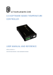
(LibReference Like '1N4*') And (HasModel('SIM','*','FALSE')) And ((LibraryName Like
'NSC*.IntLib') Or (LibraryName Like 'Motorola*.IntLib'))
Out of a possible 18000+ simulation-ready components that come installed with Altium Designer, the preceding query returns a
manageable 57 components, as illustrated by the following image.
TR0113 (v1.6) April 21, 2008
19
Simulation Models and Analyses Reference
For help on getting started with writing query expressions, refer to the Introduction to the Query Language article.
For more detailed information regarding queries, refer to the article An Insider's Guide to the Query Language.
For detailed information on query language syntax, including example query expressions for each keyword, refer to the
Query Language Reference.
For detailed information about the Libraries panel, refer to the Libraries panel section of the Altium Designer Panels
Reference.
20
TR0113 (v1.6) April 21, 2008
Simulation Models and Analyses Reference
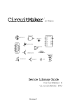
Searching via the Altium Website
By navigating to the Altium Designer Libraries area of the Altium Website, you can browse, search and download up-to-date
Altium Designer integrated libraries for board-level design. Simply click on the available link for the Altium Designer boardlevel design integrated libraries and then access the Search for a component facility. Use this facility to quickly search for
simulation-ready components.
Use the fields provided to make your search criteria as
broad or specific as required. If, for example, you wanted to
quickly find all simulation-ready components of a particular
type – across all manufacturer integrated libraries – simply
set the Class and Sub-Class fields as required and ensure
that the Show only simulation-ready components option is
enabled. Such a search could be narrowed further by
entering a specific package type for the component, and so
on.
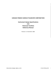
After running the search, the results will be listed,
alphabetically, and by manufacturer. The following
information is provided:
•
Component Name
•
Manufacturer of the component
•
Description of the component
•
Package Type
•
Name of the integrated library into which the component
has been compiled
•
Downloadable zip file – containing all integrated libraries
for that manufacturer
•
Date Component was last updated.
TR0113 (v1.6) April 21, 2008
21
Simulation Models and Analyses Reference
From the list of results, you can access further information about a component, simply by clicking on the entry for its name.
From a simulation perspective, this gives you information about any model or sub-circuit file linked as a model to the
component.
22
TR0113 (v1.6) April 21, 2008
Simulation Models and Analyses Reference
The Netlist Template - Explained
The Netlist Template allows access to the information that is entered into the XSpice netlist for a given component. It is
accessed by clicking on the Netlist Template tab, at the bottom of the Sim Model dialog.
For all of the predefined model kinds and sub-kinds, the Netlist Template is read-only. If, however, one of these predefined
entries does not allow enough control over the information placed in the netlist, you can define your own template.
To edit the Netlist Template, you need to select Generic Editor in the Model Sub-Kind region of the Sim Model dialog ensuring that the Model Kind field is first set to General. This will be the default model kind/sub-kind setting when adding a
new simulation model to a schematic component. For all other General model sub-kinds, you can effectively change to Generic
Editor and edit the predefined template - massaging it to your own requirements.
When defining the Netlist Template, the information entered should be in accordance with the requirements of SPICE3f5/XSpice
and the syntax rules described below.
Netlist Template Syntax
Characters that are entered into the template are written to the XSpice netlist verbatim, except for the following special
characters:
%
-
percent sign
@ -
commercial at
&
-
ampersand
?
-
question mark
~
-
tilde
#
-
number sign
These characters are translated when creating the netlist, as shown in the following table:
Syntax in Netlist Template...
Netlister replaces with...
@<param>
Value of <param>. An error is raised if a parameter of this name does not exist or if
there is no value assigned to it.
&<param>
Value of <param>. No error is raised if the parameter is undefined.
TR0113 (v1.6) April 21, 2008
23
Simulation Models and Analyses Reference
Syntax in Netlist Template...
Netlister replaces with...
?<param>s…s
Text between s…s separators if <param> is defined.
?<param>s…ss…s
Text between first s…s separators if <param> is defined, else the second s…s
separators.
~<param>s…s
Text between s…s separators if <param> is NOT defined.
~<param>s…ss…s
Text between first s…s separators if <param> is NOT defined, else the second s…s
separators.
#<param>s…s
Text between s…s separators if <param> is defined, but ignore the rest of the template
if <param> is NOT defined.
#s…s
Text between s…s separators if there is any text to be entered into the XSpice netlist
from subsequent entries in the Netlist Template.
%<pin id>
The net name of the net to which the schematic pin mapped to <pin id> connects.
%%
A literal percent character.
In the above table,
•
s represents a separator character (, . ; / |).
•
<param> refers to the name of a parameter.
If the parameter name contains any non-alphanumeric characters, it should be enclosed in double quotes. For example:
@"DC Magnitude" - double quotes used here because the name contains a space.
&"Init_Cond" - double quotes used here because the name contains an underscore.
Double quotes should also be used when you wish to add an alphanumeric prefix to a parameter name. For example:
@"DESIGNATOR"A - the use of the double quotes ensures that A is appended to the component designator.
Syntax Examples
The following are examples of the special character syntax entries in the previous table. Information is given in each case, about
how the syntax entry is translated by the Netlister.
@"AC Phase"
The parameter name AC Phase is enclosed in braces because of the space. This will be replaced in the netlist with the value of
the AC Phase parameter. If there is no parameter of this name, or its value is blank then an error will be given.
&Area
If a parameter named Area exists and has a value, then it’s value will be entered into the netlist. If the parameter is undefined
(i.e. either it does not exist or has no value assigned) then nothing will be written to the netlist, but no error will be raised. This
can be used for optional parameters.
?IC|IC=@IC|
If the parameter named IC is defined then the text within the || separators will be inserted into the netlist. For example if the
parameter IC had value 0.5 then IC=0.5 would be inserted into the netlist in place of this entry. If the parameter is undefined
then nothing will be inserted into the netlist.
?IC/IC=@IC//IC=0/
This is the same as the previous example, except that if the parameter IC is undefined then IC=0 will be inserted into the netlist.
Note also that a different separator character has been used.
~VALUE/1k/
If a parameter named VALUE is NOT defined then the text 1k will be inserted into the netlist.
~VALUE/1k//@VALUE/
This is the same as the previous example, except that if the parameter VALUE is defined then its text value will be inserted into
the netlist.
24
TR0113 (v1.6) April 21, 2008
Simulation Models and Analyses Reference
#"AC Magnitude"|AC@"AC Magnitude"|@"AC Phase"
This example can be seen in the predefined netlist template for the sinusoidal voltage source.
If the AC Magnitude parameter has been defined then the contents of the separators is evaluated and inserted into the netlist.
All following entries in the netlist are also evaluated and entered into the netlist (in this case @”AC Phase”).
If for example AC Magnitude=1 and AC Phase=0 then AC 1 0 will be inserted into the netlist. If, however, AC Phase was
undefined, an error would be raised.
If the parameter AC Magnitude is undefined then nothing following the #”AC Magnitude” entry in the netlist template will be
entered into the netlist.
#|PARAMS:|?Resistance|Resistance=Resistance|?Current|Current=@Current|
This example can be seen in the predefined netlist template for a parameterized subcircuit (see F1 in Fuse.PrjPcb).
If the Resistance and Current parameters are both undefined then there will be no text to be inserted into the netlist following
the #|PARAMS:| entry, so the text in the separators will be omitted also.
If for example the parameters have values Resistance=1k and Current=5mA then this will result in text following the
#|PARAMS:| entry and PARAMS: Resistance=1k Current=5mA will be the entry made in the netlist.
@DESIGNATOR%1%2@VALUE
This example is to demonstrate the use of the % character.
If for example the parameters have values DESIGNATOR=R1 and VALUE=1k, and the pins are mapped on the Port Map tab of
the Sim Model dialog according to the following table:
Schematic Pin
Model Pin
Net name to which Schematic Pin connects
1 (N+)
1 (1)
GND
2 (N-)
2 (2)
OUT
Then the text R1 GND OUT 1k will be placed into the XSpice netlist for this component.
Checking the Netlist Template
To check the Netlist Template, simply click on the Netlist Preview tab at the bottom of the Sim Model dialog. The text displayed
in this tab is exactly as it will be written to the XSpice netlist file when a netlist is generated or a simulation is run. The following
exception applies:
•
If you are in the Schematic Library Editor, or the document/project has not been compiled, the net names that the model pins
map to will not be available. In this case, the schematic pin designators are inserted, enclosed in <> braces.
Any errors that occur while parsing user-defined entries in the Netlist Template will also be displayed, so that any errors can be
resolved prior to exiting the dialog.
PSpice Support
To facilitate compatibility with PSpice, support for various additional PSpice-based functions and operators is provided, as well
as the use of global parameters – to represent values in a PSpice-modeled circuit.
Additional Function Support
The following additional functions are supported:
ARCTAN(x)
-
returns the inverse tangent of x
ATAN2(y, x)
-
returns the inverse tangent of y/x
IF(t, x, y)
-
If t is TRUE then x, ELSE y
LIMIT(x, min, max)
-
while min < x < max, x is returned
If x < min, min is returned
If x > max, max is returned
LOG10(x)
-
returns the decimal logarithm of x
MAX(x, y)
-
returns the maximum of x and y
MIN(x, y)
-
returns the minimum of x and y
TR0113 (v1.6) April 21, 2008
25
Simulation Models and Analyses Reference
PWR(x, y)
-
returns x to the power of y
PWRS(x, y)
-
returns signed x to the power of y:
If x > 0, the result is positive
If x < 0, the result is negative.
SCHEDULE(x1, y1,…xn, yn)
-
allows you to control the value of y based on time x. An entry for time = 0s
must be entered.
From time = x1 to x2, returns y1
From time = x2 to x3, returns y2, and so on.
SGN(x)
-
returns the sign of x (a.k.a. the signum function).
If x < 0, returns -1
If x = 0, returns 0
If x > 0, returns 1
STP(x)
-
unit step function.
If x > 0, returns 1
If x < 0, returns 0
TABLE(x, x1, y1,…xn, yn)
-
allows you to construct a look-up table, returning the y value corresponding
to x when all xn, yn points are plotted and connected by straight lines.
If x > than the largest x value in the table, then the y value associated to
that x value will be returned.
If x < than the smallest x value in the table, then the y value associated to
that x value will be returned.
Additional Operator Support
The following additional operators are supported:
•
** (exponentiation)
•
== (equality test)
•
!= (non-equality test)
•
& (Boolean AND)
•
| (Boolean OR)
.PARAM Support
The PSpice .PARAM statement is supported. This statement defines the value of a parameter, allowing you to use a parameter
name in place of numeric values for a circuit description. Parameters can be constants, expressions or a combination of the two.
A single parameter statement can include reference to one or more additional parameter statements.
In addition, the following three internal variables (predefined parameters) are available for use in expressions:
GMIN
- shunt conductance for semiconductor p-n junctions.
TEMP
- temperature.
VT
- thermal voltage.
Global Parameters
Altium Designer’s Circuit Simulator supports the use of global parameters and equations. Use a global parameter in an equation
and then use that equation in a component value on your schematic. Alternatively, define the equation as a global parameter
and then reference the global parameter from a component value.
Simply include the expression or parameter name within curly braces {} – when the Simulator detects this it will attempt to
evaluate it, checking the Global Parameters page of the Simulator’s Analyses Setup dialog for the definition of any part of the
expression that cannot be immediately resolved.
26
TR0113 (v1.6) April 21, 2008
Simulation Models and Analyses Reference
For an example of using global parameters and equations in a simulation, refer to the example project Global
Params.PrjPCB, which can be found in the \Examples\Circuit Simulation\PSpice Examples\Global
Parameters folder of the installation.
TR0113 (v1.6) April 21, 2008
27
Simulation Models and Analyses Reference
SPICE3f5 models
These are predefined analog device models that are built-in to SPICE. They cover the following, common analog component
types.
General
•
Capacitor
•
Capacitor (Semiconductor)
•
Coupled Inductors
•
Diode
•
Inductor
•
Potentiometer
•
Resistor
•
Resistor (Semiconductor)
•
Resistor (Variable)
Transistors
•
Bipolar Junction Transistor (BJT)
•
Junction Field-Effect Transistor (JFET)
•
Metal Semiconductor Field-Effect Transistor (MESFET)
•
Metal Oxide Semiconductor Field-Effect Transistor (MOSFET)
Switches
•
Current Controlled Switch
•
Voltage Controlled Switch
Transmission Lines
•
Lossless Transmission Line
•
Lossy Transmission Line
•
Uniform Distributed RC (lossy) Transmission Line
Current Sources
•
Current-Controlled Current Source
•
DC Current Source
•
Exponential Current Source
•
Frequency Modulated Sinusoidal Current Source
•
Non-Linear Dependent Current Source
•
Piecewise Linear Current Source
•
Pulse Current Source
•
Sinusoidal Current Source
•
Voltage-Controlled Current Source
Voltage Sources
•
Current-Controlled Voltage Source
•
DC Voltage Source
•
Exponential Voltage Source
•
Frequency Modulated Sinusoidal Voltage Source
•
Non-Linear Dependent Voltage Source
•
Piecewise Linear Voltage Source
•
Pulse Voltage Source
•
Sinusoidal Voltage Source
28
TR0113 (v1.6) April 21, 2008
Simulation Models and Analyses Reference
•
Voltage-Controlled Voltage Source
Initial Conditions
•
Initial Condition
•
Nodeset
Notes
Many of the models have associated model files (*.mdl). A model file is used to allow specification of specific device
parameters (e.g. on and off resistances for a switch).
Many of the above models have been modified to make them compatible with PSpice. In such cases, PSpice support
information is included as part of that model’s information, later in this reference.
Many of the component libraries (*.IntLib) that come with the installation, feature simulation-ready devices. These devices
have the necessary model or sub-circuit file included and linked to the schematic component. These are pure SPICE models for
maximum compatibility with analog simulators.
For more detailed information regarding SPICE3, consult the SPICE3f5 User Manual. There were no syntax changes made
between SPICE3f3 and SPICE3f5. The manual for SPICE3f3 therefore describes the correct syntax for the netlist and models
supported by the Altium Designer-based Mixed-Signal Simulator.
General
Capacitor
Model Kind
General
Model Sub-Kind
Capacitor
SPICE Prefix
C
SPICE Netlist Template Format
@DESIGNATOR %1 %2 @VALUE ?"INITIAL VOLTAGE"|IC=@"INITIAL VOLTAGE"|
Parameters (definable at component level)
The following component-level parameters are definable for this model type and are listed on the Parameters tab of the Sim
Model dialog. To access this dialog, simply double-click on the entry for the simulation model link in the Models region of the
Component Properties dialog.
Value
-
value for the capacitance (in Farads).
Initial Voltage
-
time-zero voltage of capacitor (in Volts).
Notes
The value for the Initial Voltage only applies if the Use Initial Conditions option is enabled on the Transient/Fourier
Analysis Setup page of the Analyses Setup dialog.
Examples
Consider the capacitor in the above image, with the following characteristics:
•
Pin1 (positive) is connected to net N1
•
Pin2 (negative) is connected to net VN
•
Designator is C1
TR0113 (v1.6) April 21, 2008
29
Simulation Models and Analyses Reference
•
Value = 0.02uF.
The entry in the SPICE netlist would be:
*Schematic Netlist:
C1 N1 VN 0.02uF
Capacitor (Semiconductor)
Model Kind
General
Model Sub-Kind
Capacitor(Semiconductor)
SPICE Prefix
C
SPICE Netlist Template Format
@DESIGNATOR %1 %2 &VALUE &MODEL ?LENGTH|L=@LENGTH| ?WIDTH|W=@WIDTH| ?"INITIAL
VOLTAGE"|IC=@"INITIAL VOLTAGE"|
Parameters (definable at component level)
The following component-level parameters are definable for this model type and are listed on the Parameters tab of the Sim
Model dialog. To access this dialog, simply double-click on the entry for the simulation model link in the Models region of the
Component Properties dialog.
Value
-
value for the capacitance (in Farads).
Length
-
length of the capacitor (in meters).
Width
-
width of the capacitor (in meters) (Default = 1e-6).
Initial Voltage
-
time-zero voltage of capacitor (in Volts).
Parameters (definable within model file)
The following is a list of process-related parameters that can be stored in the associated model file:
CJ
-
2
junction bottom capacitance (in F/meters ).
CJSW
-
junction sidewall capacitance (in F/meters).
DEFW
-
default width (in meters). - this value will be overridden by a value entered for Width in the Sim Model
dialog.
NARROW
-
narrowing due to side etching (in meters). (Default = 0).
Notes
The value for the Initial Voltage only applies if the Use Initial Conditions option is enabled on the Transient/Fourier
Analysis Setup page of the Analyses Setup dialog.
You can specify either a direct value for the capacitance OR enter values for the capacitors' length and width. In the case of the
latter, a value for the capacitance will be calculated, in conjunction with parameter information stored in the model.
The equation used to calculate the capacitance from geometric data is:
CAP = CJ(LENGTH - NARROW)(WIDTH - NARROW) + 2CJSW(LENGTH + WIDTH - 2 NARROW)
If a direct value for capacitance is not specified, the model name and length must be supplied in order for the geometric-based
capacitance value to be calculated.
The link to the required model file (*.mdl) is specified on the Model Kind tab of the Sim Model dialog. The Model Name is
used in the netlist to reference this file.
Either the direct capacitance value OR the geometric data used to calculate it can be entered, but not both.
30
TR0113 (v1.6) April 21, 2008
Simulation Models and Analyses Reference
Where a parameter has an indicated default (as part of the SPICE model definition), that default will be used if no value is
specifically entered. The default should be applicable to most simulations. Generally you do not need to change this value.
Examples
Consider the semiconductor capacitor in the above image, with the following characteristics:
•
Pin1 is connected to net N1
•
Pin2 is connected to net VN
•
Designator is C1
•
The linked simulation model file is CAP.mdl
If a value for the capacitance was entered directly, say 100 pF, and no other parameters were specified on the Parameters tab
of the Sim Model dialog, then the entry in the SPICE netlist would be:
*Schematic Netlist:
C1 N1 VN 100pF CAP
Consider now, instead of entering a direct value for the capacitance, the following parameters were defined in the Sim Model
dialog:
•
Length = 10u
•
Width = 1u
the entry in the netlist would be:
C1 N1 VN CAP L=10u W=1u
The value for the capacitance will be calculated accurately using the geometric data specified and any further parameter
definitions in the model file (CAP.mdl).
PSpice Support
To make this device model compatible with PSpice, the following additional model parameters are supported and can be
entered into a linked model file (*.mdl) for the device:
C
- capacitance multiplier. (Default = 1).
TC1
- linear temperature coefficient (in ˚C ). (Default = 0).
TC2
- quadratic temperature coefficient (in ˚C ). (Default = 0).
VC1
- linear voltage coefficient (in Volt ). (Default = 0).
VC2
- quadratic voltage coefficient (in Volt ). (Default = 0).
-1
-2
-1
-2
Where a parameter has an indicated default, that default will be used if no value is specifically
entered.
The format for the PSpice model file is:
.MODEL ModelName CAP(Model Parameters),
where
The following parameters –
common to most devices in
PSpice – are not supported:
T_ABS
T_MEASURED
•
ModelName is the name of the model, the link to which is specified on the Model Kind tab of the
T_REL_GLOBAL
Sim Model dialog. This name is used in the netlist (&MODEL) to reference the required model in
T_REL_LOCAL.
the linked model file.
•
Model Parameters are a list of supported parameters for the model, entered with values as
required.
For an example of using a PSpice-compatible capacitor model in a simulation, refer to the example project
Capacitor.PrjPCB, which can be found in the \Examples\Circuit Simulation\PSpice Examples\Capacitor
folder of the installation.
TR0113 (v1.6) April 21, 2008
31
Simulation Models and Analyses Reference
Coupled Inductors
Model Kind
General
Model Sub-Kind
Coupled Inductors
SPICE Prefix
K
SPICE Netlist Template Format
LA_@DESIGNATOR %1 %2 @"INDUCTANCE A"
LB_@DESIGNATOR %3 %4 @"INDUCTANCE B"
@DESIGNATOR LA_@DESIGNATOR LB_@DESIGNATOR @"COUPLING FACTOR"
Parameters (definable at component level)
The following component-level parameters are definable for this model type and are listed on the Parameters tab of the Sim
Model dialog. To access this dialog, simply double-click on the entry for the simulation model link in the Models region of the
Component Properties dialog.
Inductance A
-
value for the inductance of discrete inductor A (in Henrys).
Inductance B
-
value for the inductance of discrete inductor B (in Henrys).
Coupling Factor
-
the coupling coefficient, representing the flux linkage between the windings of the two individual
inductors. Permissible values lie in the range 0<CF≤1, where 1 (the ideal) means all flux linking
inductor A also links inductor B.
Examples
Consider the transformer in the above image, which uses a coupled inductor model and has the following characteristics:
•
The positive pin of the Primary is connected to net Vin2
•
The negative pin of the Primary is connected to net GND
•
The positive pin of the secondary is connected to net Vout2
•
The negative pin of the secondary is connected to net GND
•
Designator is T1
•
Inductance A = 1mH
•
Inductance B = 1mH
•
Coupling Factor = 0.5.
The entry in the SPICE netlist would be:
*Schematic Netlist:
LA_KT1 VIN2 0 1mH
LB_KT1 VOUT2 0 1mH
KT1 LA_KT1 LB_KT1 0.5
32
TR0113 (v1.6) April 21, 2008
Simulation Models and Analyses Reference
Placing a transformer with a coupled inductor model is probably the simplest and quickest way of adding a coupled inductor to
your source schematic. However, should you wish to place individual inductors in the schematic design and couple them, the
required information for the SPICE netlist can be readily supplied through the use of a Text Frame.
Simply place a text frame in the schematic document and ensure that the first line is:
.NSX
Then type the information required - each line will be included in the netlist, exactly as it is written, appearing between the
following comment entries:
*Begin NSX text frames
*End of NSX text frames
The following example illustrates the use of two inductors and a text frame to provide a coupled inductor for simulation
purposes.
Consider the circuit in the adjacent image, which contains two discrete inductors with
the following characteristics:
•
Designator (Primary inductor) = L1
•
Designator (Secondary inductor) = L2
•
The positive pin of L1 is connected to net Vin1
•
The negative pin of L1 is connected to net GND
•
The positive pin of L2 is connected to net Vout1
•
The negative pin of L2 is connected to net GND
•
Value for inductance (L1) = 10mH
•
Value for inductance (L2) = 10mH
The entries in the text frame are dissected as follows:
•
.NSX - the mandatory first line that tells the netlister that the following lines are
extra information to be added when generating the SPICE netlist.
•
K1 - the designator for the 'coupled inductor', where K is the required SPICE prefix.
•
L1, L2 - the designators of the two individual inductors
•
0.5 - the value for the Coupling Factor
The entry in the SPICE netlist would be:
*Begin NSX text frames
K1 L1 L2 0.5
*End of NSX text frames
.
.
*Schematic Netlist:
L1 VIN1 0 10mH
L2 VOUT1 0 10mH
TR0113 (v1.6) April 21, 2008
33
Simulation Models and Analyses Reference
Diode
Model Kind
General
Model Sub-Kind
Diode
SPICE Prefix
D
SPICE Netlist Template Format
@DESIGNATOR %1 %2 @MODEL &"AREA FACTOR" &"STARTING CONDITION" ?"INITIAL VOLTAGE"|IC=@"INITIAL
VOLTAGE"| ?TEMPERATURE|TEMP=@TEMPERATURE|
Parameters (definable at component level)
The following component-level parameters are definable for this model type and are listed on the Parameters tab of the Sim
Model dialog. To access this dialog, simply double-click on the entry for the simulation model link in the Models region of the
Component Properties dialog.
Area Factor
-
specifies the number of equivalent parallel devices of the specified model. This setting affects a
number of parameters in the model.
Starting Condition
-
set to OFF to set diode voltage to zero during operating point analysis. Can be useful as an aid
in convergence.
Initial Voltage
-
time-zero voltage across the diode (in Volts).
Temperature
-
temperature at which the device is to operate (in Degrees Celsius). (Default = 27).
Parameters (definable within model file)
The following is a list of parameters that can be stored in the associated model file:
IS
-
saturation current (in Amps). (Default = 1.0e-14).
RS
-
ohmic resistance (in Ohms). (Default = 0).
N
-
emission coefficient (Default = 1).
TT
-
transit-time (in seconds). (Default = 0).
CJO
-
zero-bias junction capacitance (in Farads). (Default = 0).
VJ
-
junction potential (in Volts). (Default = 1).
M
-
grading coefficient (Default = 0.5).
EG
-
activation energy (in eV). (Default = 1.11).
XTI
-
saturation-current temp exp. (Default = 3.0).
KF
-
flicker noise coefficient (Default = 0)
AF
-
flicker noise exponent (Default = 1).
FC
-
coefficient for forward-bias depletion capacitance formula (Default = 0.5).
BV
-
reverse breakdown voltage (in Volts). (Default = infinite).
IBV
-
current at breakdown voltage (in Amps). (Default = 1.0e-3).
TNOM
-
parameter measurement temperature (in °C) - If no value is specified, the default value assigned to TNOM
on the SPICE Options page of the Analyses Setup dialog will be used (Default = 27).
34
TR0113 (v1.6) April 21, 2008
Simulation Models and Analyses Reference
Notes
The value for the Initial Voltage only applies if the Use Initial Conditions option is enabled on the Transient/Fourier
Analysis Setup page of the Analyses Setup dialog.
The Area Factor affects the following three model parameters:
•
saturation current (IS)
•
ohmic resistance (RS)
•
zero-bias junction capacitance (CJO)
If the Area Factor is omitted, a value of 1.0 is assumed.
The link to the required model file (*.mdl) is specified on the Model Kind tab of the Sim Model dialog. The Model Name is
used in the netlist to reference this file.
Where a parameter has an indicated default (as part of the SPICE model definition), that default will be used if no value is
specifically entered. The default should be applicable to most simulations. Generally you do not need to change this value.
Examples
Consider the diode in the above image, with the following characteristics:
•
Pin1 (anode) is connected to net VIN
•
Pin2 (cathode) is connected to net Vhw
•
Designator is D1
•
The linked simulation model file is 1N4002.mdl.
If no values are entered for the parameters in the Sim Model dialog, the entries in the SPICE netlist would be:
*Schematic Netlist:
D1 VIN VHW 1N4002
.
.
*Models and Subcircuit:
.MODEL 1N4002 D(IS=2.55E-9 RS=0.042 N=1.75 TT=5.76E-6 CJO=1.85E-11 VJ=0.75
+ M=0.333 BV=100 IBV=1E-5 )
and the SPICE engine would use the indicated parameter information defined in the model file, along with default parameter
values inherent to the model for those parameters not specified in the file.
If the following parameter values were specified on the Parameters tab of the Sim Model dialog:
•
Area Factor = 3
•
Initial Voltage = 2
•
Temperature = 22
then the entries in the SPICE netlist would be:
*Schematic Netlist:
D1 VIN VHW 1N4002 3 IC=2 TEMP=22
.
.
*Models and Subcircuit:
.MODEL 1N4002 D(IS=2.55E-9 RS=0.042 N=1.75 TT=5.76E-6 CJO=1.85E-11 VJ=0.75
TR0113 (v1.6) April 21, 2008
35
Simulation Models and Analyses Reference
+ M=0.333 BV=100 IBV=1E-5 )
In this case, the SPICE engine would use this information, in conjunction with the indicated parameters defined in the model file
(and any defaults for parameters not specified).
PSpice Support
To make this device model compatible with PSpice, the following additional model parameters are supported and can be
entered into a linked model file (*.mdl) for the device:
IBVL
- low-level reverse breakdown knee current (in Amps). (Default = 0).
IKF
- high-injection knee current (in Amps). (Default = infinite).
ISR
- recombination current parameter (in Amps). (Default = 0).
NBV
- reverse breakdown ideality factor. (Default = 1).
NBVL
- low-level reverse breakdown ideality factor. (Default = 1).
NR
- emission coefficient for isr. (Default = 2).
TBV1
- bv temperature coefficient – linear (in ˚C ). (Default = 0).
TBV2
- bv temperature coefficient – quadratic (in ˚C ). (Default = 0).
TIKF
- ikf temperature coefficient – linear (in ˚C ). (Default = 0).
TRS1
- rs temperature coefficient – linear (in ˚C ). (Default = 0).
TRS2
- rs temperature coefficient – quadratic (in ˚C ). (Default = 0).
-1
-2
-1
-1
-2
Where a parameter has an indicated default, that default will be used if no value is specifically entered.
The format for the PSpice model file is:
.MODEL ModelName D(Model Parameters),
where
The following parameters –
common to most devices in
PSpice – are not supported:
•
ModelName is the name of the model, the link to which is specified on the Model Kind tab of the T_ABS
T_MEASURED
Sim Model dialog. This name is used in the netlist (@MODEL) to reference the required model in
T_REL_GLOBAL
the linked model file.
•
Model Parameters are a list of supported parameters for the model, entered with values as
required.
T_REL_LOCAL.
For an example of using a PSpice-compatible diode model in a simulation, refer to the example project Diode.PrjPCB,
which can be found in the \Examples\Circuit Simulation\PSpice Examples\Diode folder of the installation.
Inductor
Model Kind
General
Model Sub-Kind
Inductor
SPICE Prefix
L
SPICE Netlist Template Format
@DESIGNATOR %1 %2 @VALUE ?"INITIAL CURRENT"|IC=@"INITIAL CURRENT"|
Parameters (definable at component level)
The following component-level parameters are definable for this model type and are listed on the Parameters tab of the Sim
Model dialog. To access this dialog, simply double-click on the entry for the simulation model link in the Models region of the
Component Properties dialog.
Value
36
-
value for the inductance (in Henrys).
TR0113 (v1.6) April 21, 2008
Simulation Models and Analyses Reference
Initial Current
-
time-zero current flowing through inductor (in Amps).
Notes
The value for the Initial Current only applies if the Use Initial Conditions option is enabled on the Transient/Fourier
Analysis Setup page of the Analyses Setup dialog.
Examples
Consider the inductor in the above image, with the following characteristics:
•
Pin1 (positive) is connected to net Vin
•
Pin2 (negative) is connected to net Vfw
•
Designator is L1
•
Value = 10mH.
The entry in the SPICE netlist would be:
*Schematic Netlist:
L1 Vin Vfw 10mH
PSpice Support
The existing Spice3f5 model for the Inductor device has been
enhanced to support the general PSpice model form:
L<name> <(+) node> <(-) node> [model name]
<value> [IC = <initial value>]
A PSpice model of this type should be linked to a schematic
component using a model file. Simply specify the model in a
model file (*.mdl) then, in the Sim Model dialog, set the
Model Kind to General and the Model Sub-Kind to
Generic Editor. The Netlist Template Format should then
be entered as follows:
@DESIGNATOR %1 %2 @VALUE @MODEL ?"INITIAL
CURRENT"|IC=@"INITIAL CURRENT"|
The value for the INITIAL CURRENT parameter is entered
on the Parameters tab of the Sim Model dialog.
The netlist format for a PSpice Inductor model is specified
using the Generic Editor due to the fact that the Spice3f5
Inductor model does not support use of a linked model file.
For the circuit to be parsed correctly, ensure that the Spice Prefix field is set to L.
In the Model Name field, enter the name specified for the model in the model file. Use the options in the Model Location region
of the dialog to point to the required file. Click on the Model File tab to view the content of the model file.
The following additional model parameters are supported and can be entered into a linked model file (*.mdl) for the device:
L
- inductance multiplier. (Default = 1).
IL1
- linear current coefficient (in Amp ). (Default = 0).
IL2
- quadratic current coefficient (in Amp ). (Default = 0).
-1
TR0113 (v1.6) April 21, 2008
-2
37
Simulation Models and Analyses Reference
-1
TC1
- linear temperature coefficient (in ˚C ). (Default = 0).
TC2
- quadratic temperature coefficient (in ˚C ). (Default = 0).
-2
Where a parameter has an indicated default, that default will be used if no value is specifically
entered.
The format for the PSpice model file is:
.MODEL ModelName IND(Model Parameters),
where
The following parameters –
common to most devices in
PSpice – are not supported:
T_ABS
T_MEASURED
•
ModelName is the name of the model, the link to which is specified on the Model Kind tab of the T_REL_GLOBAL
Sim Model dialog. This name is used in the netlist (@MODEL) to reference the required model in
T_REL_LOCAL.
the linked model file.
•
Model Parameters are a list of supported parameters for the model, entered with values as
required.
For an example of using a PSpice-compatible inductor model in a simulation, refer to the example project
Inductor.PrjPCB, which can be found in the \Examples\Circuit Simulation\PSpice Examples\Inductor
folder of the installation.
Potentiometer
Model Kind
General
Model Sub-Kind
Potentiometer
SPICE Prefix
R
SPICE Netlist Template Format
@"DESIGNATOR"A %1 %2 {@VALUE * @"SET POSITION"}
@"DESIGNATOR"B %2 %3 {@VALUE - (@VALUE * @"SET POSITION")}
Parameters (definable at component level)
The following component-level parameters are definable for this model type and are listed on the Parameters tab of the Sim
Model dialog. To access this dialog, simply double-click on the entry for the simulation model link in the Models region of the
Component Properties dialog.
Value
-
value for the resistance (in Ohms).
Set Position
-
the position of the wiper along the resistors' track. The value can be in the range 0 (fully left/anticlockwise) to 1 (fully right/clockwise), with 0.5 being the halfway point, with equal resistance on
both sides.
Examples
Consider the potentiometer in the image above, with the following characteristics:
•
Pin1 (Top) is connected to net OUT
•
Pin2 (Bot) is connected to net IN
•
Pin3 (Tap or wiper) is connected to net IN
•
Designator is RIn
•
Value = 1K
•
Set Position = 0.5.
38
TR0113 (v1.6) April 21, 2008
Simulation Models and Analyses Reference
The entry in the SPICE netlist would be:
*Schematic Netlist:
RInA OUT IN {1K * 0.5}
RInB IN IN {1K – (1K * 0.5)}
Resistor
Model Kind
General
Model Sub-Kind
Resistor
SPICE Prefix
R
SPICE Netlist Template Format
@DESIGNATOR %1 %2 @VALUE
Parameters (definable at component level)
The following component-level parameters are definable for this model type and are listed on the Parameters tab of the Sim
Model dialog. To access this dialog, simply double-click on the entry for the simulation model link in the Models region of the
Component Properties dialog.
Value
-
value for the resistance (in Ohms).
Examples
Consider the resistor in the above image, with the following characteristics:
•
Pin1 (Top) is connected to net Output
•
Pin2 (Bot) is connected to net GND
•
Designator is RLoad
•
Value = 25k.
The entry in the SPICE netlist would be:
*Schematic Netlist:
RLoad OUTPUT 0 25k - the ground net is always defined as 0 in the netlist.
Resistor (Semiconductor)
Model Kind
General
Model Sub-Kind
Resistor(Semiconductor)
SPICE Prefix
R
TR0113 (v1.6) April 21, 2008
39
Simulation Models and Analyses Reference
SPICE Netlist Template Format
@DESIGNATOR %1 %2 &VALUE &MODEL ?LENGTH|L=@LENGTH| ?WIDTH|W=@WIDTH|
?TEMPERATURE|TEMP=@TEMPERATURE|
Parameters (definable at component level)
The following component-level parameters are definable for this model type and are listed on the Parameters tab of the Sim
Model dialog. To access this dialog, simply double-click on the entry for the simulation model link in the Models region of the
Component Properties dialog.
Value
-
value for the resistance (in Ohms).
Length
-
length of the resistor (in meters).
Width
-
width of the resistor (in meters). (Default = 1e-6).
Temperature
-
temperature at which the device is to operate (in Degrees Celsius). (Default = 27°C).
Parameters (definable within model file)
The following is a list of process-related parameters that can be stored in the associated model file:
TC1
-
first order temperature coefficient (in Ohms/°C). (Default = 0).
TC2
-
2
second order temperature coefficient (in Ohms/°C ). (Default = 0).
RSH
-
sheet resistance (in Ohms).
DEFW
-
default width (in meters). - this value will be overridden by a value entered for Width in the Sim Model
dialog.
NARROW
-
narrowing due to side etching (in meters). (Default = 0).
TNOM
-
parameter measurement temperature (in °C) - If no value is specified, the default value assigned to TNOM
on the SPICE Options page of the Analyses Setup dialog will be used (Default = 27).
Notes
You can specify either a direct value for the resistance OR enter values for the resistors' length and width. In the case of the
latter, a value for the resistance will be calculated, in conjunction with parameter information stored in the model.
The equation used to calculate the resistance from geometric data is:
R = RSH * ((L - NARROW) / (W - NARROW))
If a direct value for resistance is not specified, the model name and length must be supplied in order for the geometric-based
resistance value to be calculated. If either the length or sheet resistance (RSH) is not specified, the default resistance value of
1K will be used and a warning will be generated.
The link to the required model file (*.mdl) is specified on the Model Kind tab of the Sim Model dialog. The Model Name is
used in the netlist to reference this file.
Entering a direct value for the resistance will override the geometric definition.
Where a parameter has an indicated default (as part of the SPICE model definition), that default will be used if no value is
specifically entered. The default should be applicable to most simulations. Generally you do not need to change this value.
Examples
Consider the semiconductor resistor in the above image, with the following characteristics:
•
Pin1 is connected to net Input
•
Pin2 is connected to net Inv
•
Designator is RIn
•
The linked simulation model file is RES.mdl.
40
TR0113 (v1.6) April 21, 2008
Simulation Models and Analyses Reference
If a value for the resistance was entered directly, say 10K, and no other parameters were specified on the Parameters tab of
the Sim Model dialog, then the entry in the SPICE netlist would be:
*Schematic Netlist:
RIn Input Inv RES 10K
Consider now, instead of entering a direct value for the resistance, the following parameters were defined in the Sim Model
dialog:
•
Length = 10e-3
•
Width = 4e-3
•
Temperature = 24.
The entry in the netlist would be:
*Schematic Netlist:
RIn INPUT INV RES L=10e-3 W=4e-3 TEMP=24
As long as a value for the sheet resistance (RSH) has been defined in the model file (RES.mdl), the value for the resistance will
be calculated accurately from the geometric data given.
PSpice Support
The existing Spice3f5 model for the Resistor (Semiconductor) device has been enhanced to support the general PSpice model
form:
R<name> <(+) node> <(-) node> [model name] <value> [TC = <TC1> [,<TC2>]]
A PSpice model of this type should be linked to a schematic
component using a model file. Simply specify the model in a
model file (*.mdl) then, in the Sim Model dialog, set the Model
Kind to General and the Model Sub-Kind to Generic
Editor. The Netlist Template Format should then be entered
as follows:
@DESIGNATOR %1 %2 &MODEL &VALUE
?TC1/TC=@TC1?TC2|, @TC2| /
Although you could use the Spice3f5 Resistor (Semiconductor)
model – as this model type allows use of a linked model file –
specification of the netlist format for a PSpice Resistor model
using the Generic Editor allows you to make use of the
additional PSpice parameters ([TC = <TC1> [,<TC2>]]).
For the circuit to be parsed correctly, ensure that the Spice
Prefix field is set to R.
In the Model Name field, enter the name specified for the
model in the model file. Use the options in the Model Location
region of the dialog to point to the required file. Click on the
Model File tab to view the content of the model file.
The following additional model parameters are supported and
can be entered into a linked model file (*.mdl) for the device:
R
- resistance multiplier. (Default = 1).
TC1
- linear temperature coefficient (in ˚C ). (Default = 0).
TC2
- quadratic temperature coefficient (in ˚C ). (Default = 0).
TCE
- exponential temperature coefficient (in %/˚C). (Default =
0).
-1
-2
Values for TC1 and TC2 can be entered on the Parameters tab of the Sim Model dialog. Where a parameter has an indicated
default, that default will be used if no value is specifically entered – either on the Parameters tab or in the linked model file.
The format for the PSpice model file is:
.MODEL ModelName RES(Model Parameters),
TR0113 (v1.6) April 21, 2008
41
Simulation Models and Analyses Reference
where
•
ModelName is the name of the model, the link to which is specified on the Model Kind tab of the
Sim Model dialog. This name is used in the netlist (&MODEL) to reference the required model in
The following parameters –
the linked model file.
common to most devices in
•
Model Parameters are a list of supported parameters for the model, entered with values as
required.
For an example of using a PSpice-compatible capacitor model in a simulation, refer to the
example project Resistor.PrjPCB, which can be found in the \Examples\Circuit
Simulation\PSpice Examples\Resistor folder of the installation.
PSpice – are not supported:
T_ABS
T_MEASURED
T_REL_GLOBAL
T_REL_LOCAL.
Resistor (Variable)
Model Kind
General
Model Sub-Kind
Resistor(Variable)
SPICE Prefix
R
SPICE Netlist Template Format
@DESIGNATOR %1 %2 {@VALUE * @"SET POSITION"}
Parameters (definable at component level)
The following component-level parameters are definable for this model type and are listed on the Parameters tab of the Sim
Model dialog. To access this dialog, simply double-click on the entry for the simulation model link in the Models region of the
Component Properties dialog.
Value
Set Position
value for the resistance (in Ohms).
-
the position of the wiper along the resistors' track. The value can be in the range 0 (fully left/anticlockwise) to 1 (fully right/clockwise), with 0.5 being the halfway point (i.e. the resistors' value will be
half that specified in the Value field).
Examples
Consider the variable resistor in the image above, with the following characteristics:
•
Pin1 is connected to net Input
•
Pin2 is connected to net Inv
•
Designator is R1
•
Value = 1K
•
Set Position = 0.5.
The entry in the SPICE netlist would be:
*Schematic Netlist:
R1 INPUT INV 5E+2
Transistors
Bipolar Junction Transistor (BJT)
Model Kind
Transistor
42
TR0113 (v1.6) April 21, 2008
Simulation Models and Analyses Reference
Model Sub-Kind
BJT
SPICE Prefix
Q
SPICE Netlist Template Format
@DESIGNATOR %1 %2 %3 @MODEL &"AREA FACTOR" &"STARTING CONDITION" ?"INITIAL B-E
VOLTAGE"|IC=@"INITIAL B-E VOLTAGE", @"INITIAL C-E VOLTAGE"| ?TEMPERATURE|TEMP=@TEMPERATURE|
Parameters (definable at component level)
The following component-level parameters are definable for this model type and are listed on the Parameters tab of the Sim
Model dialog. To access this dialog, simply double-click on the entry for the simulation model link in the Models region of the
Component Properties dialog.
Area Factor
-
specifies the number of equivalent parallel devices of the specified model. This setting
affects a number of parameters in the model.
Starting Condition
-
set to OFF to set terminal voltages to zero during operating point analysis. Can be useful as
an aid in convergence.
Initial B-E Voltage
-
time-zero voltage across base-emitter terminals (in Volts).
Initial C-E Voltage
-
time-zero voltage across collector-emitter terminals (in Volts).
Temperature
-
temperature at which the device is to operate (in Degrees Celsius). If no value is specified,
the default value assigned to TEMP on the SPICE Options page of the Analyses Setup
dialog will be used (Default = 27).
Parameters (definable within model file)
The following is a list of parameters that can be stored in the associated model file:
IS
-
transport saturation current (in Amps). (Default = 1.0e-16).
BF
-
ideal maximum forward beta (Default = 100).
NF
-
forward current emission coefficient (Default = 1).
VAF
-
forward Early voltage (in Volts). (Default = infinite).
IKF
-
corner for forward beta high current roll-off (in Amps). (Default = infinite).
ISE
-
B-E leakage saturation current (in Amps). (Default = 0).
NE
-
B-E leakage emission coefficient (Default = 1.5).
BR
-
ideal maximum reverse beta (Default = 1).
NR
-
reverse current emission coefficient (Default = 1).
VAR
-
reverse Early voltage (in Volts). (Default = infinite).
IKR
-
corner for reverse beta high current roll-off (in Amps). (Default = infinite).
ISC
-
B-C leakage saturation current (in Amps). (Default = 0).
NC
-
B-C leakage emission coefficient (Default = 2).
RB
-
zero bias base resistance (in Ohms). (Default = 0).
IRB
-
current where base resistance falls halfway to it minimum value (in Amps). (Default = infinite).
RBM
-
minimum base resistance at high currents (in Ohms). (Default = RB).
RE
-
emitter resistance (in Ohms). (Default = 0).
TR0113 (v1.6) April 21, 2008
43
Simulation Models and Analyses Reference
RC
-
collector resistance (in Ohms). (Default = 0).
CJE
-
B-E zero-bias depletion capacitance (in Farads). (Default = 0).
VJE
-
B-E built-in potential (in Volts). (Default = 0.75)
MJE
-
B-E junction exponential factor (Default = 0.33).
TF
-
ideal forward transit time (in seconds). (Default = 0).
XTF
-
coefficient for bias dependence of TF (Default = 0).
VTF
-
voltage describing VBC dependence of TF (in Volts). (Default = infinite).
ITF
-
high-current parameter for effect on TF (in Amps). (Default = 0).
PTF
-
excess phase at freq=1.0/(TF*2PI) Hz (in Degrees). (Default = 0).
CJC
-
B-C zero-bias depletion capacitance (in Farads). (Default = 0).
VJC
-
B-C built-in potential (in Volts). (Default = 0.75).
MJC
-
B-C junction exponential factor (Default = 0.33).
XCJC
-
fraction of B-C depletion capacitance connected to internal base node (Default = 1).
TR
-
ideal reverse transit time (in seconds). (Default = 0).
CJS
-
zero-bias collector-substrate capacitance (in Farads). (Default = 0).
VJS
-
substrate junction built-in potential (in Volts). (Default = 0.75).
MJS
-
substrate junction exponential factor (Default = 0).
XTB
-
forward and reverse beta temperature exponent (Default = 0).
EG
-
energy gap for temperature effect on IS (in eV). (Default = 1.11).
XTI
-
temperature exponent for effect on IS (Default = 3).
KF
-
flicker noise coefficient (Default = 0).
AF
-
flicker noise exponent (Default = 1).
FC
-
coefficient for forward-bias depletion capacitance formula (Default = 0.5).
TNOM
-
parameter measurement temperature (in °C) - If no value is specified, the default value assigned to TNOM on
the SPICE Options page of the Analyses Setup dialog will be used (Default = 27).
Notes
The model for the BJT is an adaptation of the integral charge control model of Gummel and Poon. This enhanced version of the
original Gummel-Poon model includes several effects at high bias levels. When certain parameters are not specified, the model
automatically defaults to that of the simpler Ebers-Moll model.
Ground is used as the substrate node.
The values for Initial B-E Voltage and Initial C-E Voltage only apply if the Use Initial Conditions option is
enabled on the Transient/Fourier Analysis Setup page of the Analyses Setup dialog.
The Area Factor affects the following model parameters:
•
transport saturation current (IS)
•
corner for forward beta high current roll-off (IKF)
•
B-E leakage saturation current (ISE)
•
corner for reverse beta high current roll-off (IKR)
•
B-C leakage saturation current (ISC)
•
zero bias base resistance (RB)
44
TR0113 (v1.6) April 21, 2008
Simulation Models and Analyses Reference
•
current where base resistance falls halfway to its minimum value (IRB)
•
minimum base resistance at high currents (RBM)
•
emitter resistance (RE)
•
collector resistance (RC)
•
B-E zero-bias depletion capacitance (CJE)
•
high-current parameter for effect on TF (ITF)
•
B-C zero-bias depletion capacitance (CJC)
•
zero-bias collector-substrate capacitance (CJS)
If the Area Factor is omitted, a value of 1.0 is assumed.
The link to the required model file (*.mdl) is specified on the Model Kind tab of the Sim Model dialog. The Model Name is
used in the netlist to reference this file.
Where a parameter has an indicated default (as part of the SPICE model definition), that default will be used if no value is
specifically entered. The default should be applicable to most simulations. Generally you do not need to change this value.
Examples
Consider the BJT in the above image, with the following characteristics:
•
Pin1 (collector) is connected to net C
•
Pin2 (base) is connected to net GND
•
Pin3 (emitter) is connected to net E
•
Designator is Q1
•
The linked simulation model file is 2N3904.mdl.
If no values are entered for the parameters in the Sim Model dialog, the entries in the SPICE netlist would be:
*Schematic Netlist:
Q1 C 0 E 2N3904
.
.
*Models and Subcircuit:
.MODEL 2N3904 NPN(IS=1.4E-14 BF=300 VAF=100 IKF=0.025 ISE=3E-13 BR=7.5 RC=2.4
+ CJE=4.5E-12 TF=4E-10 CJC=3.5E-12 TR=2.1E-8 XTB=1.5 KF=9E-16 )
and the SPICE engine would use the indicated parameter information defined in the model file, along with default parameter
values inherent to the model for those parameters not specified in the file.
If the following parameter values were specified on the Parameters tab of the Sim Model dialog:
•
Area Factor = 3
•
Starting Condition = OFF
•
Temperature = 24
then the entries in the SPICE netlist would be:
*Schematic Netlist:
TR0113 (v1.6) April 21, 2008
45
Simulation Models and Analyses Reference
Q1 C 0 E 2N3904 3 OFF
TEMP=24
.
.
*Models and Subcircuit:
.MODEL 2N3904 NPN(IS=1.4E-14 BF=300 VAF=100 IKF=0.025 ISE=3E-13 BR=7.5 RC=2.4
+ CJE=4.5E-12 TF=4E-10 CJC=3.5E-12 TR=2.1E-8 XTB=1.5 KF=9E-16 )
In this case, the SPICE engine would use this information, in conjunction with the indicated parameters defined in the model file
(and any defaults for parameters not specified).
PSpice Support
Many of the parameters that can be included in a linked model file for this type of device are common to both Spice3f5 and
PSpice. Those that are supported can be found in the previous section – Parameters (definable within model file). The following
PSpice-based parameters are not supported for this device type:
CN
-
quasi-saturation temperature coefficient for hole mobility
D
-
quasi-saturation temperature coefficient for
scattering-limited hole carrier velocity
GAMMA
-
epitaxial region doping factor
ISS
-
substrate p-n saturation current
NK
-
high-current roll-off coefficient
NS
-
substrate p-n emission coefficient
QCO
-
epitaxial region charge factor
QUASIMOD
-
quasi-saturation model flag for temperature dependence
RCO
-
epitaxial region resistance
TRB1
-
RB temperature coefficient (linear)
TRB2
-
RB temperature coefficient (quadratic)
TRC1
-
RC temperature coefficient (linear)
TRC2
-
RC temperature coefficient (quadratic)
TRE1
-
RE temperature coefficient (linear)
TRE2
-
RE temperature coefficient (quadratic)
TRM1
-
RBM temperature coefficient (linear)
TRM2
-
RBM temperature coefficient (quadratic)
VG
-
quasi-saturation extrapolated bandgap voltage at 0° K
VO
-
carrier mobility knee voltage
XCJC2
-
fraction of CJC connected internally to Rb
XCJS
-
fraction of CJS connected internally to Rc
Junction Field-Effect Transistor (JFET)
Model Kind
Transistor
Model Sub-Kind
JFET
SPICE Prefix
J
46
TR0113 (v1.6) April 21, 2008
Simulation Models and Analyses Reference
SPICE Netlist Template Format
@DESIGNATOR %1 %2 %3 @MODEL &"AREA FACTOR" &"STARTING CONDITION" ?"INITIAL D-S
VOLTAGE"|IC=@"INITIAL D-S VOLTAGE", @"INITIAL G-S VOLTAGE"| ?TEMPERATURE|TEMP=@TEMPERATURE|
Parameters (definable at component level)
The following component-level parameters are definable for this model type and are listed on the Parameters tab of the Sim
Model dialog. To access this dialog, simply double-click on the entry for the simulation model link in the Models region of the
Component Properties dialog.
Area Factor
-
specifies the number of equivalent parallel devices of the specified model. This setting
affects a number of parameters in the model.
Starting Condition
-
set to OFF to set terminal voltages to zero during operating point analysis. Can be useful as
an aid in convergence.
Initial D-S Voltage
-
time-zero voltage across Drain-Source terminals (in Volts).
Initial G-S Voltage
-
time-zero voltage across Gate-Source terminals (in Volts).
Temperature
-
temperature at which the device is to operate (in Deg. C). If no value is specified, the default
value assigned to TEMP on the SPICE Options page of the Analyses Setup dialog will be
used (Default = 27).
Parameters (definable within model file)
The following is a list of parameters that can be stored in the associated model file:
VTO
-
threshold voltage VTO (in Volts). (Default = -2.0).
BETA
-
2
transconductance parameter β (in A/V ). (Default = 1.0e-4)
LAMBDA
-
channel-length modulation parameter λ (in 1/V). (Default = 0).
RD
-
drain ohmic resistance (in Ohms). (Default = 0).
RS
-
source ohmic resistance (in Ohms). (Default = 0).
CGS
-
zero-bias G-S junction capacitance CGS (in Farads). (Default = 0).
CGD
-
zero-bias G-D junction capacitance CGD (in Farads). (Default = 0).
PB
-
gate junction potential (in Volts). (Default = 1).
IS
-
gate junction saturation current IS (in Amps). (Default = 1.0e-14).
B
-
doping tail parameter (Default = 1).
KF
-
flicker noise coefficient (Default = 0).
AF
-
flicker noise exponent (Default = 1).
FC
-
coefficient for forward-bias depletion capacitance formula (Default = 0.5).
TNOM
-
parameter measurement temperature (in °C) - If no value is specified, the default value assigned to TNOM
on the SPICE Options page of the Analyses Setup dialog will be used (Default = 27).
Notes
The model for the JFET is based on the FET model of Shichman and Hodges.
The values for the Initial D-S Voltage and Initial G-S Voltage only apply if the Use Initial Conditions option is
enabled on the Transient/Fourier Analysis Setup page of the Analyses Setup dialog.
The Area Factor affects the following model parameters:
•
transconductance parameter (BETA)
•
drain ohmic resistance (RD)
•
source ohmic resistance (RS)
TR0113 (v1.6) April 21, 2008
47
Simulation Models and Analyses Reference
•
zero-bias G-S junction capacitance (CGS)
•
zero-bias G-D junction capacitance (CGD)
•
gate junction saturation current (IS).
If the Area Factor is omitted, a value of 1.0 is assumed.
The link to the required model file (*.mdl) is specified on the Model Kind tab of the Sim Model dialog. The Model Name is
used in the netlist to reference this file.
Where a parameter has an indicated default (as part of the SPICE model definition), that default will be used if no value is
specifically entered. The default should be applicable to most simulations. Generally you do not need to change this value.
Examples
Consider the JFET in the above image, with the following characteristics:
•
Pin1 (Drain) is connected to net D
•
Pin2 (Gate) is connected to net G
•
Pin3 (Source) is connected to net S
•
Designator is J1
•
The linked simulation model file is 2N4393.mdl.
If no values are entered for the parameters in the Sim Model dialog, the entries in the SPICE netlist would be:
*Schematic Netlist:
J1 D G S 2N4393
.
.
*Models and Subcircuit:
.MODEL 2N4393 NJF(VTO=-1.422 BETA=0.009109 LAMBDA=0.006 RD=1 RS=1 CGS=4.06E-12
+ CGD=4.57E-12 IS=2.052E-13 KF=1.23E-16 )
and the SPICE engine would use the indicated parameter information defined in the model file, along with default parameter
values inherent to the model for those parameters not specified in the file.
If the following parameter values were specified on the Parameters tab of the Sim Model dialog:
•
Area Factor = 4
•
Temperature = 29
then the entries in the SPICE netlist would be:
*Schematic Netlist:
J1 D G S 2N4393 4
TEMP=29
.
.
*Models and Subcircuit:
48
TR0113 (v1.6) April 21, 2008
Simulation Models and Analyses Reference
.MODEL 2N4393 NJF(VTO=-1.422 BETA=0.009109 LAMBDA=0.006 RD=1 RS=1 CGS=4.06E-12
+ CGD=4.57E-12 IS=2.052E-13 KF=1.23E-16 )
In this case, the SPICE engine would use this information, in conjunction with the indicated parameters defined in the model file
(and any defaults for parameters not specified).
PSpice Support
To make this device model compatible with PSpice, the following additional model parameters are supported and can be
entered into a linked model file (*.mdl) for the device:
-1
ALPHA
-
ionization coefficient (in Volt ). (Default = 0).
BETATCE
-
BETA exponential temperature coefficient (in Amp/Volt ). (Default = 1E-4).
ISR
-
gate p-n recombination current parameter (in Amps). (Default = 0).
M
-
gate p-n grading coefficient. (Default = 0.5).
N
-
gate p-n emission coefficient. (Default = 1).
NR
-
emission coefficient for isr. (Default = 2).
VK
-
ionization knee voltage (in Volts). (Default = 0).
VTOTC
-
VTO temperature coefficient (in Volt/˚C). (Default = 0).
XTI
-
IS temperature coefficient. (Default = 3).
2
Where a parameter has an indicated default, that default will be used if no value is specifically
entered.
The format for the PSpice model file is:
.MODEL ModelName NJF(Model Parameters) – N-channel JFET
.MODEL ModelName PJF(Model Parameters) – P-channel JFET
where
The following parameters –
common to most devices in
PSpice – are not supported:
T_ABS
T_MEASURED
T_REL_GLOBAL
•
ModelName is the name of the model, the link to which is specified on the Model Kind tab of the T_REL_LOCAL.
Sim Model dialog. This name is used in the netlist (@MODEL) to reference the required model in
the linked model file.
•
Model Parameters are a list of supported parameters for the model, entered with values as required.
For an example of using a PSpice-compatible diode model in a simulation, refer to the example project JFET.PrjPCB,
which can be found in the \Examples\Circuit Simulation\PSpice Examples\Jfet folder of the installation.
Metal Semiconductor Field-Effect Transistor (MESFET)
Model Kind
Transistor
Model Sub-Kind
MESFET
SPICE Prefix
Z
SPICE Netlist Template Format
@DESIGNATOR %1 %2 %3 @MODEL &"AREA FACTOR" &"STARTING CONDITION" ?"INITIAL D-S
VOLTAGE"|IC=@"INITIAL D-S VOLTAGE", @"INITIAL G-S VOLTAGE"|
Parameters (definable at component level)
The following component-level parameters are definable for this model type and are listed on the Parameters tab of the Sim
Model dialog. To access this dialog, simply double-click on the entry for the simulation model link in the Models region of the
Component Properties dialog.
Area Factor
TR0113 (v1.6) April 21, 2008
-
specifies the number of equivalent parallel devices of the specified model. This setting
49
Simulation Models and Analyses Reference
affects a number of parameters in the model.
Starting Condition
-
set to OFF to set terminal voltages to zero during operating point analysis. Can be useful as
an aid in convergence.
Initial D-S Voltage
-
time-zero voltage across Drain-Source terminals (in Volts).
Initial G-S Voltage
-
time-zero voltage across Gate-Source terminals (in Volts).
Parameters (definable within model file)
The following is a list of parameters that can be stored in the associated model file:
VTO
-
pinch-off voltage (in Volts). (Default = -2.0).
BETA
-
2
transconductance parameter β (in A/V ). (Default = 1.0e-4)
B
-
doping tail extending parameter (in 1/V). (Default = 0.3).
ALPHA
-
saturation voltage parameter (in 1/V). (Default = 2).
LAMBDA
-
channel-length modulation parameter λ (in 1/V). (Default = 0).
RD
-
drain ohmic resistance (in Ohms). (Default = 0).
RS
-
source ohmic resistance (in Ohms). (Default = 0).
CGS
-
zero-bias G-S junction capacitance (in Farads). (Default = 0).
CGD
-
zero-bias G-D junction capacitance (in Farads). (Default = 0).
PB
-
gate junction potential (in Volts). (Default = 1).
KF
-
flicker noise coefficient (Default = 0).
AF
-
flicker noise exponent (Default = 1).
FC
-
coefficient for forward-bias depletion capacitance formula (Default = 0.5).
Notes
The model for the MESFET is based on the GaAs FET model of Statz et-al.
The values for the Initial D-S Voltage and Initial G-S Voltage only apply if the Use Initial Conditions option is
enabled on the Transient/Fourier Analysis Setup page of the Analyses Setup dialog.
The Area Factor affects the following model parameters:
•
transconductance parameter (BETA)
•
doping tail extending parameter (B)
•
saturation voltage parameter (ALPHA)
•
drain ohmic resistance (RD)
•
source ohmic resistance (RS)
•
zero-bias G-S junction capacitance (CGS)
•
zero-bias G-D junction capacitance (CGD).
If the Area Factor is omitted, a value of 1.0 is assumed.
The link to the required model file (*.mdl) is specified on the Model Kind tab of the Sim Model dialog. The Model Name is
used in the netlist to reference this file.
Where a parameter has an indicated default (as part of the SPICE model definition), that default will be used if no value is
specifically entered. The default should be applicable to most simulations. Generally you do not need to change this value.
50
TR0113 (v1.6) April 21, 2008
Simulation Models and Analyses Reference
Examples
Consider the MESFET in the above image, with the following characteristics:
•
Pin1 (Drain) is connected to net D
•
Pin2 (Gate) is connected to net G
•
Pin3 (Source) is connected to net S
•
Designator is Q1
•
The linked simulation model file is NMESFET.mdl.
If no values are entered for the parameters in the Sim Model dialog, the entries in the SPICE netlist would be:
*Schematic Netlist:
ZQ1 D G S NMESFET
.
.
*Models and Subcircuit:
.MODEL NMESFET NMF(LEVEL=6, )
In this case, there are no parameter values specified in both the Sim Model dialog and the model file. The SPICE engine would
therefore use the parameter default values inherent to the model.
Metal Oxide Semiconductor Field-Effect Transistor (MOSFET)
Model Kind
Transistor
Model Sub-Kind
MOSFET
SPICE Prefix
M
SPICE Netlist Template Format
@DESIGNATOR %1 %2 %3 %3 @MODEL ?LENGTH|L=@LENGTH| ?WIDTH|W=@WIDTH| ?"DRAIN AREA"|AD=@"DRAIN
AREA"| ?"SOURCE AREA"|AS=@"SOURCE AREA"| ?"DRAIN PERIMETER"|PD=@"DRAIN PERIMETER"| ?"SOURCE
PERIMETER"|PS=@"SOURCE PERIMETER"| ?NRD|NRD=@NRD| ?NRS|NRS=@NRS| &"STARTING CONDITION"
?"INITIAL D-S VOLTAGE"|IC=@"INITIAL D-S VOLTAGE", @"INITIAL G-S VOLTAGE", @"INITIAL B-S
VOLTAGE"| ?TEMPERATURE|TEMP=@TEMPERATURE|
TR0113 (v1.6) April 21, 2008
51
Simulation Models and Analyses Reference
Parameters (definable at component level)
The following component-level parameters are definable for this model type and are listed on the Parameters tab of the Sim
Model dialog. To access this dialog, simply double-click on the entry for the simulation model link in the Models region of the
Component Properties dialog.
Length
-
channel length (in meters).
Width
-
channel width (in meters).
Drain Area
-
area of the Drain diffusion (in sq.meters).
Source Area
-
area of the Source diffusion (in sq.meters).
Drain Perimeter
-
perimeter of drain junction (in meters). (Default = 0).
Source Perimeter
-
perimeter of source junction (in meters). (Default = 0).
NRD
-
equivalent number of squares of the drain diffusion (Default = 1).
NRS
-
equivalent number of squares of the source diffusion (Default = 1).
Starting Condition
-
set to OFF to set terminal voltages to zero during operating point analysis. Can be
useful as an aid in convergence.
Initial D-S Voltage
-
time-zero voltage across Drain-Source terminals (in Volts).
Initial G-S Voltage
-
time-zero voltage across Gate-Source terminals (in Volts).
Initial B-S Voltage
-
time-zero voltage across Bulk (substrate)-Source terminals (in Volts).
Temperature
-
temperature at which the device is to operate (in Degrees Celsius). If no value is
specified, the default value assigned to TEMP on the SPICE Options page of the
Analyses Setup dialog will be used (Default = 27).
M
-
multiplication factor. (Default = 1). This parameter is only available when using the
EKV model.
Parameters (definable within model file)
The following is a list of parameters that can be stored in the associated model file, when using the Shichman-Hodges, MOS2,
MOS3 or MOS6 models:
LEVEL
-
model index (Default = 1).
VTO
-
zero-bias threshold voltage VTO (in Volts). (Default = 0).
KP
-
2
transconductance parameter (in A/V ). (Default = 2.0e-5).
GAMMA
-
1/2
bulk threshold parameter γ (in V ). (Default = 0).
PHI
-
surface potential φ (in Volts). (Default = 0.6).
LAMBDA
-
channel length modulation λ (in 1/V). This parameter is applicable to MOS1 and MOS2 model types only.
(Default = 0).
RD
-
drain ohmic resistance (in Ohms). (Default = 0).
RS
-
source ohmic resistance (in Ohms). (Default = 0).
CBD
-
zero-bias B-D junction capacitance (in Farads). (Default = 0).
CBS
-
zero-bias B-S junction capacitance (in Farads). (Default = 0).
IS
-
bulk junction saturation current IS (in Amps). (Default = 1.0e-14).
PB
-
bulk junction potential (in Volts). (Default = 0.8).
CGSO
-
Gate-Source overlap capacitance per meter channel width (in Farads per meter). (Default = 0).
52
TR0113 (v1.6) April 21, 2008
Simulation Models and Analyses Reference
CGDO
-
Gate-Drain overlap capacitance per meter channel width (in Farads per meter). (Default = 0).
CGBO
-
Gate-Bulk overlap capacitance per meter channel length (in Farads per meter). (Default = 0).
RSH
-
Drain and Source diffusion sheet resistance (in Ohms). (Default = 0).
CJ
-
2
zero-bias bulk junction bottom capacitance per square meter of junction area (in Farads/m ). (Default =
0).
MJ
-
bulk junction bottom grading coefficient (Default = 0.5).
CJSW
-
zero-bias bulk junction sidewall capacitance per meter of junction perimeter (in Farads/meter). (Default =
0).
MJSW
-
bulk junction sidewall grading coefficient (Default = 0.5 - LEVEL1; 0.33 - LEVEL2,3).
JS
-
2
bulk junction saturation current per square meter of junction area (in Amps/m ).
TOX
-
oxide thickness (in meters). (Default = 1.0e-7).
NSUB
-
3
substrate doping (in 1/cm ). (Default = 0).
NSS
-
2
surface state density (in 1/cm ). (Default = 0).
NFS
-
2
fast surface state density (in 1/cm ). (Default = 0).
TPG
-
type of gate material:
+1 (default) = opposite to substrate
-1 = same as substrate
0 = Al gate
XJ
-
metallurgical junction depth (in meters). (Default = 0). This applies to Levels 2 (MOS2) and 3 (MOS3)
only.
LD
-
lateral diffusion (in meters). (Default = 0).
UO
-
2
surface mobility (in cm /Vs). (Default = 600).
UCRIT
-
critical field for mobility degradation (in V/cm). This parameter is applicable to the MOS2 model only.
(Default = 1.0e4).
UEXP
-
critical field exponent in mobility degradation. This parameter is applicable to the MOS2 model only.
(Default = 0).
UTRA
-
transverse field coefficient (mobility). This parameter has been deleted with respect to the MOS2 model.
(Default = 0).
VMAX
-
maximum drift velocity of carriers (in m/s). (Default = 0).
NEFF
-
total channel-charge (fixed and mobile) coefficient. This parameter is applicable to the MOS2 model only.
(Default = 1).
KF
-
flicker noise coefficient (Default = 0).
AF
-
flicker noise exponent (Default = 1).
FC
-
coefficient for forward-bias depletion capacitance formula (Default = 0.5).
DELTA
-
width effect on threshold voltage. This parameter is applicable to MOS2 and MOS3 model types only.
(Default = 0).
THETA
-
mobility modulation (in 1/V). This parameter is applicable to the MOS3 model only. (Default = 0).
ETA
-
static feedback. This parameter is applicable to the MOS3 model only. (Default = 0).
KAPPA
-
saturation field factor. This parameter is applicable to the MOS3 model only. (Default = 0.2).
TR0113 (v1.6) April 21, 2008
53
Simulation Models and Analyses Reference
TNOM
-
parameter measurement temperature (in °C) - If no value is specified, the default value assigned to
TNOM on the SPICE Options page of the Analyses Setup dialog will be used (Default = 27).
The following is a list of parameters that can be stored in the associated model file, when using the BSIM or BSIM2 models:
LEVEL
-
model index (Default = 1).
VFB*
-
flat-band voltage (in Volts).
PHI*
-
surface inversion potential (in Volts).
K1*
-
1/2
body effect coefficient (in V ).
K2*
-
Drain/Source depletion charge-sharing coefficient.
ETA*
-
zero-bias drain-induced barrier-lowering coefficient.
MUZ
-
2
zero-bias mobility (in cm /Vs).
DL
-
shortening of channel (in μm).
DW
-
narrowing of channel (in μm).
U0*
-
-1
zero-bias transverse-field mobility degradation coefficient (in V ).
U1*
-
zer0-bias velocity saturation coefficient (in μm/V).
X2MZ*
-
2 2
sens. of mobility to substrate bias at Vds=0 (in cm /V s).
X2E*
-
-1
sens. of drain-induced barrier lowering effect to substrate bias (in V ).
X3E*
-
-1
sens. of drain-induced barrier lowering effect to drain bias at Vds=Vdd (in V ).
X2U0*
-
-2
sens. of transverse field mobility degradation effect to substrate bias (in V ).
X2U1*
-
-2
sens. of velocity saturation effect to substrate bias (in μmV ).
MUS
-
2 2
mobility at zero substrate bias and at Vds=Vdd (in cm /V s).
X2MS*
-
2 2
sens. of mobility to substrate bias at Vds=Vdd (in cm /V s).
X3MS*
-
2 2
sens. of mobility to drain bias at Vds=Vdd (in cm /V s).
X3U1*
-
-2
sens. of velocity saturation effect on drain bias at Vds=Vdd (in μmV ).
TOX
-
gate oxide thickness (in μm).
TEMP
-
temperature at which parameters were measured (in °C)
VDD
-
measurement bias range (in Volts).
CGDO
-
gate-drain overlap capacitance per meter channel width (in F/m).
CGSO
-
gate-source overlap capacitance per meter channel width (in F/m).
CGBO
-
gate-bulk overlap capacitance per meter channel length (in F/m).
XPART
-
gate-oxide capacitance-charge model flag.
N0*
-
zero-bias sub-threshold slope coefficient.
NB*
-
sens. of sub-threshold slope to substrate bias.
ND*
-
sens. of sub-threshold slope to drain bias.
RSH
-
drain and source diffusion sheet resistance (in Ohms).
JS
-
2
source drain junction current density (in A/m ).
PB
-
built-in potential of source drain junction (in Volts).
54
TR0113 (v1.6) April 21, 2008
Simulation Models and Analyses Reference
MJ
-
grading coefficient of source drain junction.
PBSW
-
built-in potential of source drain junction sidewall (in Volts).
MJSW
-
grading coefficient of source drain junction sidewall.
CJ
-
2
source drain junction capacitance per unit area (in F/m ).
CJSW
-
source drain junction sidewall capacitance per unit length (in F/m).
WDF
-
source drain junction default width (in meters).
DELL
-
source drain junction length reduction (in meters).
The following is a list of parameters that can be stored in the associated model file, when using the BSIM3 model:
LEVEL
-
model index (Default = 1).
MOBMOD
-
mobility model selector (Default = 1).
CAPMOD
-
flag for the short-channel capacitance model (Default = 2).
NQSMOD
-
flag for NQS model (Default = 0).
NOIMOD
-
flag for noise model (Default = 1).
VTH0
-
threshold voltage (at VBS=0) for Large L (in Volts). (Default = 0.7 – NMOS; -0.7 – PMOS). (See BSIM3Related notes).
K1
-
first-order body effect coefficient (in V1/2). (Default = 0.5). (See BSIM3-Related notes).
K2
-
second-order body effect coefficient (Default = 0). (See BSIM3-Related notes).
K3
-
narrow width coefficient (Default = 80).
K3B
-
body effect coefficient of K3 (in 1/V). (Default = 0).
W0
-
narrow width parameter (in meters) (Default = 2.5e-6).
NLX
-
lateral non-uniform doping parameter (in meters). (Default = 1.74e-7).
VBM
-
maximum applied body bias in Vth calculation (in Volts). (Default = -3.0).
DVT0
-
first coefficient of short-channel effect on Vth (Default = 2.2).
DVT1
-
second coefficient of short-channel effect on Vth (Default = 0.53).
DVT2
-
body-bias coefficient of short-channel effect on Vth (in 1/V). (Default = -0.032).
DVT0W
-
first coefficient of narrow width effect on Vth for small channel length (in 1/m). (Default = 0).
DVT1W
-
second coefficient of narrow width effect on Vth for small channel length (in 1/m). (Default = 5.3e6).
DVT2W
-
body-bias coefficient of narrow width effect for small channel length (in 1/V). (Default = -0.032).
U0
-
mobility at TEMP = TNOM (in cm2/V/s). (Default = 670.0 – NMOSFET; 250.0 – PMOSFET).
UA
-
first-order mobility degradation coefficient (in m/V). (Default = 2.25e-9).
UB
-
second-order mobility degradation coefficient (in (m/V)2). (Default = 5.87e-19).
UC
-
body-effect of mobility degradation coefficient.
2
For MOBMOD = 1 or 2, measured in m/V , Default = -4.65e-11
For MOBMOD = 3, measured in 1/V, Default = -0.046.
VSAT
-
saturation velocity at TEMP = TNOM (in m/sec). (Default = 8.0e4).
A0
-
bulk charge effect coefficient for channel length (Default = 1.0).
AGS
-
gate bias coefficient of Abulk (in 1/V). (Default = 0).
B0
-
bulk charge effect coefficient for channel width (in meters). (Default = 0).
TR0113 (v1.6) April 21, 2008
55
Simulation Models and Analyses Reference
B1
-
bulk charge effect width offset (in meters). (Default = 0).
KETA
-
body-bias coefficient of bulk charge effect (in 1/V). (Default = -0.047).
A1
-
first non-saturation effect parameter (in 1/V). (Default = 0).
A2
-
second non-saturation factor (Default = 1).
RDSW
-
parisitic resistance per unit width (in Ω-μm
PRWB
-
body effect coefficient of RDSW (in V-1/2). (Default = 0).
PRWG
-
gate bias effect coefficient of RDSW (in 1/V). (Default = 0).
WR
-
width offset from Weff for RDS calculation (Default = 1).
WINT
-
width offset fitting parameter from I-V without bias (in meters). (Default = 0).
LINT
-
length offset fitting parameter from I-V without bias (in meters). (Default = 0).
DWG
-
coefficient of Weff's gate dependence (in m/V). (Default = 0).
DWB
-
coefficient of Weff's substrate body-bias dependence (in m/V1/2). (Default = 0).
VOFF
-
offset voltage in the subthreshold region at large W and L (in Volts). (Default = -0.08).
NFACTOR
-
subthreshold swing factor (Default = 1).
ETA0
-
DIBL coefficient in subthreshold region (Default = 0.08).
ETAB
-
body-bias coefficient for the subthreshold DIBL effect (in 1/V). (Default = -0.07).
DSUB
-
DIBL coefficient exponent in subthreshold region (Default = DROUT).
CIT
-
interface trap capacitance (in F/m2). (Default = 0).
CDSC
-
Drain/Source to channel coupling capacitance (in F/m2). (Default = 2.4e-4).
CDSCB
-
body-bias sensitivity of CDSC (in F/Vm2). (Default = 0).
CDSCD
-
Drain-bias sensitivity of CDSC (in F/Vm2). (Default = 0).
PCLM
-
channel length modulation parameter (Default = 1.3).
PDIBLC1
-
first output resistance DIBL effect correction parameter (Default = 0.39).
PDIBLC2
-
second output resistance DIBL effect correction parameter (Default = 0.0086).
PDIBLCB
-
body-effect coefficient of DIBL correction parameters (in 1/V). (Default = 0).
DROUT
-
L dependence coefficient of the DIBL correction parameter in Rout (Default = 0.56).
PSCBE1
-
first substrate current body-effect parameter (in V/m). (Default = 4.24e8).
PSCBE2
-
second substrate current body-effect parameter (in m/V). (Default = 1.0e-5).
PVAG
-
gate dependence of Early voltage (Default = 0).
DELTA
-
Effective Vds parameter (in Volts). (Default = 0.01).
NGATE
-
poly gate doping concentration (in cm-3). (Default = 0).
ALPHA0
-
the first parameter of impact ionization current (in m/V). (Default = 0).
BETA0
-
the second parameter of impact ionization current (in Volts). (Default = 30).
RSH
-
source drain sheet resistance (in Ω/square). (Default = 0).
JS
-
source drain junction saturation current per unit area (in A/m2). (Default = 1.0e-4).
XPART
-
charge partitioning rate flag (Default = 0).
CGSO
-
non LDD region source-gate overlap capacitance per channel length (in F/m). (See BSIM3-Related notes).
CGDO
-
non LDD region drain-gate overlap capacitance per channel length (in F/m). (See BSIM3-Related notes).
56
WR
). (Default = 0).
TR0113 (v1.6) April 21, 2008
Simulation Models and Analyses Reference
CGBO
-
gate bulk overlap capacitance per unit channel length (in F/m). (Default = 0).
CJ
-
2
bottom junction capacitance per unit area (in F/m ). (Default = 5e-4).
MJ
-
bottom junction capacitance grating coefficient (Default = 0.5).
MJSW
-
Source/Drain side junction capacitance grading coefficient (Default = 0.33).
CJSW
-
Source/Drain side junction capacitance per unit area (in F/m). (Default = 5e-10).
CJSWG
-
Source/Drain gate sidewall junction capacitance grading coefficient (in F/m). (Default = CJSW).
MJSWG
-
Source/Drain gate sidewall junction capacitance coefficient. (Default = MJSW).
PBSW
-
Source/Drain side junction built-in potential (in Volts). (Default = 1.0).
PB
-
bottom built-in potential (in Volts). (Default = 1.0).
PBSWG
-
Source/Drain gate sidewall junction built-in potential (in Volts). (Default = PBSW).
CKAPPA
-
coefficient for lightly doped region overlap capacitance (in F/m). (Default = 0.6).
CF
-
Fringing field capacitance (in F/m). (See BSIM3-Related notes).
CLC
-
constant term for the short channel model (in meters). (Default = 0.1e-6).
CLE
-
exponential term for the short channel model (Default = 0.6).
DLC
-
length offset fitting parameter from C-V (in meters). (Default = LINT).
DWC
-
width offset fitting parameter from C-V (in meters). (Default = WINT).
ELM
-
Elmore constant of the channel (Default = 5).
WL
-
coefficient of length dependence for width offset (in mWLN). (Default = 0).
WLN
-
power of length dependence for width offset (Default = 1.0).
WW
-
coefficient of width dependence for width offset (in mWWN). (Default = 0).
WWN
-
power of width dependence for width offset (Default = 1.0).
WWL
-
coefficient of length and width cross term for width offset (in mWWN+WLN). (Default = 0).
LL
-
coefficient of length dependence for length offset (in mLLN). (Default = 0).
LLN
-
power of length dependence for length offset (Default = 1.0).
LW
-
coefficient of width dependence for length offset (in m
LWN
-
power of width dependence for length offset (Default = 1.0).
LWL
-
coefficient of length and width cross term for length offset (in mLWN+LLN). (Default = 0).
TNOM
-
parameter measurement temperature (in °C) - If no value is specified, the default value assigned to TNOM
on the SPICE Options page of the Analyses Setup dialog will be used (Default = 27).
UTE
-
mobility temperature exponent (Default = -1.5).
KT1
-
temperature coefficient for threshold voltage (in Volts). (Default = -0.11).
KT1L
-
channel length dependence of the temperature coefficient for threshold voltage (in V*m). (Default = 0).
KT2
-
body-bias coefficient of Vth temperature effect (Default = 0.022).
UA1
-
temperature coefficient for UA (in m/V). (Default = 4.31e-9).
UB1
-
temperature coefficient for UB (in (m/V)2). (Default = -7.61e-18).
UC1
-
temperature coefficient for UC.
LWN
). (Default = 0).
2
For MOBMOD = 1 or 2, measured in m/V , Default = -5.6e-11
For MOBMOD = 3, measured in 1/V, Default = -0.056.
AT
-
temperature coefficient for saturation velocity (in m/s). (Default = 3.3e4).
TR0113 (v1.6) April 21, 2008
57
Simulation Models and Analyses Reference
PRT
-
temperature coefficient for RDSW (in Ω-μm). (Default = 0).
NJ
-
emission coefficient of junction (Default = 1).
XTI
-
junction current temperature exponent coefficient (Default = 3.0).
NOIA
-
noise parameter A (Default = 1e20 – NMOS; 9.9e18 – PMOS).
NOIB
-
noise parameter B (Default = 5e4 – NMOS; 2.4e3 – PMOS).
NOIC
-
noise parameter C (Default = -1.4e-12 – NMOS; 1.4e-12 – PMOS).
EM
-
saturation field (in V/m). (Default = 4.1e7).
AF
-
frequency exponent (Default = 1).
EF
-
flicker exponent (Default = 1).
KF
-
flicker noise parameter (Default = 0).
TOX
-
gate oxide thickness (in meters). (Default = 1.5e-8).
XJ
-
junction depth (in meters). (Default = 1.5e-7).
GAMMA1
-
1/2
body-effect coefficient near the surface (in V ). (See BSIM3-Related notes).
GAMMA2
-
body-effect coefficient in the bulk (in V1/2). (See BSIM3-Related notes).
NCH
-
channel doping concentration (in 1/cm3). (Default = 1.7e17). (See BSIM3-Related notes).
NSUB
-
substrate doping concentration (in 1/cm3). (Default = 6e16).
VBX
-
Vbs at which the depletion region width equals XT (in Volts). (See BSIM3-Related notes).
XT
-
doping depth (in meters). (Default = 1.55e-7).
LMIN
-
minimum channel length (in meters). (Default = 0).
LMAX
-
maximum channel length (in meters). (Default = 1.0).
WMIN
-
minimum channel width (in meters). (Default = 0).
WMAX
-
maximum channel width (in meters). (Default = 1.0).
BINUNIT
-
Bin unit scale selector (Default = 1).
The following is a list of parameters that can be stored in the associated model file, when using the EKV model:
Process Related Parameters
COX
-
2
gate oxide capacitance per unit area (in F/m ). (Default = 0.7e-3).
XJ
-
junction depth (in meters). (Default = 0.1e-6).
DW
-
channel width correction (in meters). (Default = 0).
DL
-
channel length correction (in meters). (Default = 0).
Basic Intrinsic Model Parameters
VTO
-
long-channel threshold voltage (in Volts). (Default = 0.5).
GAMMA
-
1/2
body effect parameter (in V ). (Default = 1.0).
PHI
-
bulk Fermi potential (*2) (in Volts). (Default = 0.7).
KP
-
transconductance parameter (in A/V2). (Default = 50.0e-6).
E0 (EO)
-
mobility reduction coefficient (in V/m). (Default = 1.0e12).
UCRIT
-
longitudinal critical field (in V/m). (Default = 2.0e6).
Optional Parameters
TOX
58
-
oxide thickness (in meters).
TR0113 (v1.6) April 21, 2008
Simulation Models and Analyses Reference
NSUB
-
-3
channel doping (in cm ).
VFB
-
flat-band voltage (in Volts).
UO
-
low-field mobility (in cm2/Vs).
VMAX
-
saturation velocity (in m/s).
THETA
-
mobility reduction coefficient (in 1/V). (Default = 0).
Channel Length Modulation and Charge Sharing Parameters
LAMBDA
-
depletion length coefficient (channel length modulation). (Default = 0.5).
WETA
-
narrow-channel effect coefficient. (Default = 0.25).
LETA
-
short-channel effect coefficient. (Default = 0.1).
Reverse Short-Channel Effect Parameters
Q0 (QO)
-
2
reverse short-channel effect peak charge density (in As/m ). (Default = 0).
LK
-
reverse short-channel effect characteristic length (in meters). (Default = 0.29e-6).
Impact Ionization Related Parameters
IBA
-
first impact ionization coefficient (in 1/m). (Default = 0).
IBB
-
second impact ionization coefficient (in V/m). (Default = 3.0e8).
IBN
-
saturation voltage factor for impact ionization. (Default = 1.0).
Intrinsic Model Temperature Parameters
TCV
-
threshold voltage temperature coefficient (in V/K). (Default = 1.0e-3).
BEX
-
mobility temperature exponent. (Default = -1.5).
UCEX
-
longitudinal critical field temperature exponent. (Default = 0.8).
IBBT
-
temperature coefficient for IBB (in 1/K). (Default = 9.0e-4).
Flicker Noise Parameters
KF
-
flicker noise coefficient. (Default = 0).
AF
-
flicker noise exponent. (Default = 1).
Setup Parameters
NQS
-
non-quasi-static (NQS) operation switch. (Default = 0).
SATLIM
-
ratio defining the saturation limit. (Default = exp(4)).
Additional Parameters
LEVEL
-
model index (Default = 1).
TNOM
-
parameter measurement temperature (in °C) - If no value is specified, the default value assigned to TNOM
on the SPICE Options page of the Analyses Setup dialog will be used (Default = 27).
IS
-
bulk junction saturation current (in Amps). (Default = 1.0e-14).
JS
-
2
bulk junction saturation current per square meter of junction area (in Amps/m ).
JSW
-
sidewall saturation current per unit length (in A/m). (Default = 0).
N
-
bulk p-n emission coefficient. (Default = 1).
CBD
-
zero-bias B-D junction capacitance (in Farads). (Default = 0).
TR0113 (v1.6) April 21, 2008
59
Simulation Models and Analyses Reference
CBS
-
zero-bias B-S junction capacitance (in Farads). (Default = 0).
CJ
-
2
zero-bias bulk junction bottom capacitance per square meter of junction area (in Farads/m ). (Default = 0).
CJSW
-
zero-bias bulk junction sidewall capacitance per meter of junction perimeter (in Farads/meter). (Default =
0).
MJ
-
bulk junction bottom grading coefficient. (Default = 0.5).
MJSW
-
bulk junction sidewall grading coefficient. (Default = 0.33).
FC
-
coefficient for forward-bias depletion capacitance formula. (Default = 0.5).
PB
-
bulk junction potential (in Volts). (Default = 0.8).
PBSW
-
built-in potential of source drain junction sidewall (in Volts). (Default = 1).
TT
-
bulk p-n transit time (in seconds). (Default = 0).
CGSO
-
Gate-Source overlap capacitance per meter channel width (in F/m). (Default = 0).
CGDO
-
Gate-Drain overlap capacitance per meter channel width (in F/m). (Default = 0).
CGBO
-
Gate-Bulk overlap capacitance per meter channel length (in F/m). (Default = 0).
RD
-
drain ohmic resistance (in Ohms). (Default = 0).
RS
-
source ohmic resistance (in Ohms). (Default = 0).
RSH
-
Drain and Source diffusion sheet resistance (in Ohms). (Default = 0).
RSC
-
source contact resistance (in Ohms). (Default = 0).
RDC
-
drain contact resistance (in Ohms). (Default = 0).
XTI
-
drain, source junction current temperature exponent. (Default = 0).
TR1
-
first-order temperature coefficient for drain, source series resistance (in °C-1). (Default = 0).
TR2
-
second-order temperature coefficient for drain, source series resistance (in °C-1). (Default = 0).
ACM
-
area calculation model. (Default = 0).
CJGATE
-
zero-bias gate-edge sidewall junction capacitance (in F/m). If no value is specified, the value assigned to
CJSW will be used. This parameter is only used when ACM = 3. It is ignored otherwise.
GEO
-
shared geometry parameter. (Default = 0). This parameter is only used when ACM = 3. It is ignored
otherwise.
HDIF
-
length of heavily doped diffusion (in m). (Default = 0). This parameter is only used when ACM = 2 or 3. It is
ignored otherwise.
LD
-
lateral diffusion into channel (in m). (Default = 0).
LDIF
-
length of lightly doped diffusion near gate (in m). (Default = 0).
SCALM
-
model scaling factor. (Default = 1).
UPDATE
-
selects effective drain and source resistance model. (Default = 0). This parameter is only used when ACM
= 1. It is ignored otherwise.
WMLT
-
width diffusion layer shrink reduction factor. (Default = 1).
Notes
General
The Simulator supports the following MOSFET device models, which differ only in their formulation of the I-V characteristic:
•
Shichman-Hodges (LEVEL=1)
•
MOS2 (LEVEL=2)
•
MOS3 (LEVEL=3)
•
BSIM (LEVEL=4)
60
TR0113 (v1.6) April 21, 2008
Simulation Models and Analyses Reference
•
BSIM2 (LEVEL=5)
•
MOS6 (LEVEL=6)
•
BSIM3 (LEVEL=7)
•
EKV (LEVEL=8).
The LEVEL parameter is used to specify which model to use. It is declared at the start of the parameter values list, entered in
the associated model file. If no LEVEL parameter is declared, the default Schichman-Hodges model will be used.
The Bulk (substrate) node is connected, by default, to the Source node.
If any of the component-level Length, Width, Drain Area or Source Area parameters are not specified, default values will
be used.
The values for the component-level NRD and NRS parameters are used to multiply the sheet resistance (RSH), in order to obtain
an accurate representation of the parasitic series drain and source resistance of each transistor.
The values for the component-level parameters Initial D-S Voltage, Initial G-S Voltage and Initial B-S
Voltage only apply if the Use Initial Conditions option is enabled on the Transient/Fourier Analysis Setup page of the
Analyses Setup dialog.
The component-level Temperature parameter applies to LEVEL 1,2,3,6 & 8 MOSFET models (not BSIM type models).
The link to the required model file (*.mdl) is specified on the Model Kind tab of the Sim Model dialog. The Model Name is
used in the netlist to reference this file.
Where a parameter has an indicated default (as part of the SPICE model definition), that default will be used if no value is
specifically entered. The default should be applicable to most simulations. Generally you do not need to change this value.
BSIM/BSIM2-Related
The BSIM and BSIM2 models are designed to be used with a process characterization system. This system is responsible for
providing all parameter information (values) automatically through the use of a process file and therefore no default parameter
values are specified. As a consequence, all parameters are required to be specified and the absence of any will result in an
error.
If the XPART parameter is set to 0, a 40/60 drain/source charge partition in saturation is selected. If this parameter is set to 1, a
0/100 drain/source charge partition is selected.
Certain model parameters (those marked with an asterisk in the BSIM/BSIM2 list of parameters) also have corresponding
parameters dependent on length and width. For more information on these and other aspects of the MOSFET models, consult
the SPICE reference manual.
BSIM3-Related
The following charge partition schemes are supported, selectable based on the value entered for the XPART parameter:
•
XPART = 0 – a 0/100 drain/source charge partition os selected
•
XPART = 0.5 – a 50/50 drain/source charge partition os selected
•
XPART = 1 – a 40/60 drain/source charge partition os selected.
If no value is specified for one of the following parameters, it will be calculated:
•
VTH0
•
K1
•
K2
•
CGSO
•
CGDO
•
CF
•
GAMMA1
•
GAMMA2
•
NCH
•
VBX
For details of the calculations involved, refer to the BSIM3v3 User Manual.
The following BSIM3 model parameters are not supported in Altium Designer:
JSSW
-
side wall saturation current density.
TR0113 (v1.6) April 21, 2008
61
Simulation Models and Analyses Reference
CGS1
-
light doped source-gate region overlap capacitance.
CGD1
-
light doped drain-gate region overlap capacitance.
VFB
-
flat-band volatge parameter.
EKV-Related
The EKV MOSFET model was developed by the Electronics Laboratory (LEG) of the Swiss Federal Institute of Technology
(EPFL). The model used in Altium Designer is version 2.6.
The following EKV model parameters are not supported in Altium Designer:
M or NP
-
parallel multiple device number.
N or NS
-
series multiple device number.
AVTO
-
area related threshold voltage mismatch parameter.
AKP
-
area related gain mismatch parameter.
AGAMMA
-
area related body effect mismatch parameter.
XQC
-
charge/capacitance model selector.
For more detailed information on model equations associated with the EKV MOSFET, refer to the document "The EPFL-EKV
MOSFET Model Equations for Simulation", available from the following website - http://legwww.epfl.ch/ekv/model.html.
Examples
Consider the MOSFET in the above image, with the following characteristics:
•
Pin1 (Drain) is connected to net D
•
Pin2 (Gate) is connected to net G
•
Pin3 (Source) is connected to net S
•
The substrate node (Bulk) is connected to Pin3 (the Source node).
•
Designator is Q1
•
The linked simulation model file is NMOS3.mdl.
If no values are entered for the parameters in the Sim Model dialog, the entries in the SPICE netlist would be:
*Schematic Netlist:
MQ1 D G S S NMOS3
.
.
*Models and Subcircuit:
62
TR0113 (v1.6) April 21, 2008
Simulation Models and Analyses Reference
.MODEL NMOS3 NMOS(LEVEL=3)
In this case, there are no parameter values specified in the Sim Model dialog. In the model file, there is only the LEVEL
parameter specified - corresponding to the use of the MOS3 model. The default values for all other parameters - inherent to the
model - will be used.
PSpice Support
Of the existing MOSFET device models, the following are not supported with respect to PSpice compatibility:
•
BSIM3 model version 2.0
For the other supported MOSFET device models, many of the parameters that can be included in a linked model file are
common to both Spice3f5 and PSpice. Those that are supported can be found in the previous section – Parameters (definable
within model file). The following PSpice-based parameters are not supported for this device type.
GDSNOI
-
channel shot noise coefficient (use with NLEV=3)
JSSW
-
bulk p-n saturation sidewall current/length
L
-
channel length
N
-
bulk p-n emission coefficient
NLEV
-
noise equation selector
PBSW
-
bulk p-n sidewall potential
RB
-
bulk ohmic resistance
RDS
-
drain-source shunt resistance
RG
-
gate ohmic resistance
TT
-
bulk p-n transit time
W
-
channel width
Switches
Current Controlled Switch
Model Kind
Switch
Model Sub-Kind
Current-Controlled
SPICE Prefix
W
SPICE Netlist Template Format
V@DESIGNATOR %1 %2 0V
@DESIGNATOR %3 %4 V@DESIGNATOR @MODEL &"INITIAL CONDITION"
Parameters (definable at component level)
The following component-level parameters are definable for this model type and are listed on the Parameters tab of the Sim
Model dialog. To access this dialog, simply double-click on the entry for the simulation model link in the Models region of the
Component Properties dialog.
Initial Condition
-
TR0113 (v1.6) April 21, 2008
the starting point for the switch, either open (OFF) or closed (ON).
63
Simulation Models and Analyses Reference
Parameters (definable within model file)
The following is a list of parameters that can be stored in the associated model file:
IT
-
threshold current (in Amps). (Default = 0).
IH
-
hysteresis current (in Amps). (Default = 0).
RON
-
ON resistance (in Ohms). (Default = 1).
ROFF
-
OFF resistance (in Ohms). (Default = 1/GMIN). GMIN is an advanced SPICE option that sets the minimum
conductance (maximum resistance) of any device in the circuit. It is specified on the Spice Options page
of the Analyses Setup dialog and its default value is 1.0e-12 (mhos).
Notes
The model allows an almost ideal switch to be described. With careful selection of the ON and OFF resistances, they can
effectively be seen as zero and infinity respectively, in comparison with other elements in the circuit.
The use of an ideal, highly non-linear element such as a switch can cause large discontinuities to occur in the circuit node
voltages. The rapid state change caused by opening and closing a switch can cause numerical round off or tolerance problems,
leading to time step difficulties, or erroneous results. When using switches, take the following precautions:
•
Set switch impedances (RON and ROFF) just high or low enough to be negligible with respect to other elements.
•
When modeling real devices such as MOSFETS, set the on resistance to a realistic level for the size of the device being
modeled.
•
If a wide range of ON to OFF resistance must be used (ROFF/RON >1e+12), then the error tolerance during transient
analysis should be decreased. Set the TRTOL parameter on the Spice Options page of the Analyses Setup dialog to 1.
•
When a switch is placed around a capacitor, then the CHGTOL parameter should also be reduced (try 1e-16).
The link to the required model file (*.mdl) is specified on the Model Kind tab of the Sim Model dialog. The Model Name is
used in the netlist to reference this file.
Where a parameter has an indicated default (as part of the SPICE model definition), that default will be used if no value is
specifically entered. The default should be applicable to most simulations. Generally you do not need to change this value.
The simulation-ready current controlled switch component (ISW) can be found in the Simulation Special Function integrated
library (\Library\Simulation\Simulation Special Function.IntLib).
Examples
Consider the current controlled switch in the above image, with the following characteristics:
•
Pin1 (positive controlling node) is connected to net IN
•
Pin2 (negative controlling node) is connected to net GND
•
Pin3 (positive output node) is connected to net NetRLY1_4 (pin 4 of RLY1).
•
Pin4 (negative output node) is connected to net IN
•
Designator is S1
•
Initial Condition of switch is OFF (open contact).
•
The linked simulation model file is ISW.mdl.
64
TR0113 (v1.6) April 21, 2008
Simulation Models and Analyses Reference
The entries in the SPICE netlist would be:
*Schematic Netlist:
VWS1 NetRLY1_4 IN 0V
WS1 IN 0 VWS1 ISW OFF
.
.
*Models and Subcircuit:
.MODEL ISW CSW()
The SPICE engine would use the value for the Initial Condition specified on the Parameters tab of the Sim Model dialog.
As there are no parameter values specified in the model file, the engine will use the default values for all other parameters.
PSpice Support
To make this device model compatible with PSpice, the following additional model parameters are supported and can be
entered into a linked model file (*.mdl) for the device:
IOFF
- control current for OFF state (in Amps). (Default = 0).
ION
- control current for ON state (in Amps). (Default = 1E-3).
Where a parameter has an indicated default, that default will be used if no value is specifically entered.
The format for the PSpice model file is:
.MODEL ModelName ISWITCH(Model Parameters),
where
The following parameters –
common to most devices in
PSpice – are not supported:
T_ABS
•
ModelName is the name of the model, the link to which is specified on the Model Kind tab of the
T_MEASURED
Sim Model dialog. This name is used in the netlist (@MODEL) to reference the required model in
T_REL_GLOBAL
the linked model file.
•
Model Parameters are a list of supported parameters for the model, entered with values as
required.
T_REL_LOCAL.
Voltage Controlled Switch
Model Kind
Switch
Model Sub-Kind
Voltage-Controlled
SPICE Prefix
S
SPICE Netlist Template Format
@DESIGNATOR %3 %4 %1 %2 @MODEL &"INITIAL CONDITION"
Parameters (definable at component level)
The following component-level parameters are definable for this model type and are listed on the Parameters tab of the Sim
Model dialog. To access this dialog, simply double-click on the entry for the simulation model link in the Models region of the
Component Properties dialog.
Initial Condition
-
TR0113 (v1.6) April 21, 2008
the starting point for the switch, either open (OFF) or closed (ON).
65
Simulation Models and Analyses Reference
Parameters (definable within model file)
The following is a list of parameters that can be stored in the associated model file:
VT
-
threshold voltage (in Volts). (Default = 0).
VH
-
hysteresis voltage (in Volts). (Default = 0).
RON
-
ON resistance (in Ohms). (Default = 1).
ROFF
-
OFF resistance (in Ohms). (Default = 1/GMIN). GMIN is an advanced SPICE option that sets the minimum
conductance (maximum resistance) of any device in the circuit. It is specified on the Spice Options page
of the Analyses Setup dialog and its default value is 1.0e-12 (mhos).
Notes
The model allows an almost ideal switch to be described. With careful selection of the ON and OFF resistances, they can
effectively be seen as zero and infinity respectively, in comparison with other elements in the circuit.
The use of an ideal, highly non-linear element such as a switch can cause large discontinuities to occur in the circuit node
voltages. The rapid state change caused by opening and closing a switch can cause numerical round off or tolerance problems,
leading to time step difficulties, or erroneous results. When using switches, take the following precautions:
•
Set switch impedances (RON and ROFF) just high or low enough to be negligible with respect to other elements.
•
When modeling real devices such as MOSFETS, set the on resistance to a realistic level for the size of the device being
modeled.
•
If a wide range of ON to OFF resistance must be used (ROFF/RON >1e+12), then the error tolerance during transient
analysis should be decreased. Set the TRTOL parameter on the Spice Options page of the Analyses Setup dialog to 1.
•
When a switch is placed around a capacitor, then the CHGTOL parameter should also be reduced (try 1e-16).
The link to the required model file (*.mdl) is specified on the Model Kind tab of the Sim Model dialog. The Model Name is
used in the netlist to reference this file.
Where a parameter has an indicated default (as part of the SPICE model definition), that default will be used if no value is
specifically entered. The default should be applicable to most simulations. Generally you do not need to change this value.
The simulation-ready voltage controlled switch component (VSW) can be found in the Simulation Special Function integrated
library (\Library\Simulation\Simulation Special Function.IntLib).
Examples
Consider the voltage controlled switch in the above image, with the following characteristics:
•
Pin1 (positive controlling node) is connected to net IN
•
Pin2 (negative controlling node) is connected to net GND
•
Pin3 (positive output node) is connected to net NetRLY1_4 (pin 4 of RLY1).
•
Pin4 (negative output node) is connected to net IN
•
Designator is S1
•
Initial Condition of switch is OFF (open contact).
•
The linked simulation model file is VSW.mdl.
66
TR0113 (v1.6) April 21, 2008
Simulation Models and Analyses Reference
The entries in the SPICE netlist would be:
*Schematic Netlist:
S1 NetRLY1_4 IN IN 0 VSW OFF
.
.
*Models and Subcircuit:
.MODEL VSW SW()
The SPICE engine would use the value for the Initial Condition specified on the Parameters tab of the Sim Model dialog.
As there are no parameter values specified in the model file, the engine will use the default values for all other parameters.
PSpice Support
To make this device model compatible with PSpice, the following additional model parameters are supported and can be
entered into a linked model file (*.mdl) for the device:
VOFF
- control voltage for OFF state (in Volts). (Default = 0).
VON
- control voltage for ON state (in Volts). (Default = 1).
Where a parameter has an indicated default, that default will be used if no value is specifically entered.
The format for the PSpice model file is:
.MODEL ModelName VSWITCH(Model Parameters),
where
The following parameters –
common to most devices in
PSpice – are not supported:
T_ABS
•
ModelName is the name of the model, the link to which is specified on the Model Kind tab of the
T_MEASURED
Sim Model dialog. This name is used in the netlist (@MODEL) to reference the required model in
T_REL_GLOBAL
the linked model file.
•
Model Parameters are a list of supported parameters for the model, entered with values as
required.
T_REL_LOCAL.
For an example of using a PSpice-compatible voltage-controlled switch model in a simulation, refer to the example project
PSpice Switch.PrjPCB, which can be found in the \Examples\Circuit Simulation\PSpice Examples\PSpice
switch folder of the installation.
Transmission Lines
Lossless Transmission Line
Model Kind
Transmission Line
Model Sub-Kind
Lossless
SPICE Prefix
T
SPICE Netlist Template Format
@DESIGNATOR %1 %2 %3 %4 Z0=@"CHAR. IMPEDANCE" ?"TRANSMISSION DELAY"/TD=@"TRANSMISSION
DELAY"//F=@FREQUENCY ?"NORMALISED LENGTH"|NL=@"NORMALISED LENGTH"|/ ?"INITIAL VOLTAGE
1"|IC=@"INITIAL VOLTAGE 1", @"INITIAL CURRENT 1", @"INITIAL VOLTAGE 2", @"INITIAL CURRENT 2"|
Parameters (definable at component level)
The following component-level parameters are definable for this model type and are listed on the Parameters tab of the Sim
Model dialog. To access this dialog, simply double-click on the entry for the simulation model link in the Models region of the
Component Properties dialog.
Char. Impedance
-
characteristic impedance (in Ohms). (Default = 50).
Transmission Delay
-
Transmission delay (in seconds). (Default = 10n).
TR0113 (v1.6) April 21, 2008
67
Simulation Models and Analyses Reference
Frequency
-
frequency (in Hertz).
Normalised Length
-
normalized electrical length of the transmission line with respect to the wavelength in
the line, at the specified frequency.
Port 1 Voltage
-
time-zero voltage at port 1 of the transmission line (in Volts).
Port 1 Current
-
time-zero current at port 1 of the transmission line (in Amps).
Port 2 Voltage
-
time-zero voltage at port 2 of the transmission line (in Volts).
Port 2 Current
-
time-zero current at port 2 of the transmission line (in Amps).
Notes
The length of the line must be expressed in one of the following two ways:
•
the Transmission Delay is specified directly (eg, TD=10ns)
•
a value for the Frequency is specified, together with a value for the Normalised Length.
If a value for Frequency is specified but a value for the Normalised Length is omitted, then 0.25 is assumed (that is, the
frequency is assumed to be the quarter-wave frequency).
The values for Port 1 and Port 2 Initial Voltages and Currents only apply if the Use Initial Conditions option is enabled on the
Transient/Fourier Analysis Setup page of the Analyses Setup dialog.
The simulation-ready lossless transmission line component (LLTRA) can be found in the Simulation Transmission Line
integrated library (\Library\Simulation\Simulation Transmission Line.IntLib).
Examples
Consider the lossless transmission line in the above image, with the following characteristics:
•
Pin1 (positive node of Port 1) is connected to net IN
•
Pin2 (negative node of Port 1) is connected to net GND
•
Pin3 (positive node of Port 2) is connected to net OUT
•
Pin4 (negative node of Port 2) is connected to net GND
•
Designator is LLTR1
•
Char. Impedance = 50Ohms
•
Transmission Delay = 20ns.
The entry in the SPICE netlist would be:
*Schematic Netlist:
TLLTR1 IN 0 OUT 0 Z0=50 TD=20NS
Lossy Transmission Line
Model Kind
Transmission Line
Model Sub-Kind
Lossy
SPICE Prefix
O
68
TR0113 (v1.6) April 21, 2008
Simulation Models and Analyses Reference
SPICE Netlist Template Format
@DESIGNATOR %1 %2 %3 %4 @MODEL
Parameters (definable at component-level)
It is not possible to pass parameter information directly from the schematic component. The parameters must be defined in the
associated model file.
Parameters (definable within model file)
The following is a list of parameters that can be stored in the associated model file:
R
-
resistance per unit length (in Ohms/unit). (Default = 0).
L
-
inductance per unit length (in Henrys/unit). (Default = 0).
G
-
conductance per unit length (in mhos/unit). (Default = 0).
C
-
capacitance per unit length (in Farads/unit). (Default = 0).
LEN
-
length of transmission line.
REL
-
breakpoint control (in arbitrary units). (Default = 1).
ABS
-
breakpoint control (in arbitrary units). (Default = 1).
NOSTEPLIMIT
-
a flag that, when set, will remove the restriction of limiting time-steps to less than the line delay.
(Default = not set).
NOCONTROL
-
a flag that, when set, prevents limiting of the time-step, based on convolution error criteria.
(Default = not set).
LININTERP
-
a flag that, when set, will use linear interpolation instead of the default quadratic interpolation,
for calculation of delayed signals. (Default = not set).
MIXEDINTERP
-
a flag that, when set, uses a metric for determining whether quadratic interpolation is applicable
and, if it isn't, uses linear interpolation. (Default = not set).
COMPACTREL
-
a specific quantity used to control the compaction of past history values used for convolution.
By default, this quantity uses the value specified for the relative simulation error tolerance
(RELTOL), which is defined on the Spice Options page of the Analyses Setup dialog.
COMPACTABS
-
a specific quantity used to control the compaction of past history values used for convolution.
By default, this quantity uses the value specified for the absolute current error tolerance
(ABSTOL), which is defined on the Spice Options page of the Analyses Setup dialog.
TRUNCNR
-
a flag that, when set, turns on the use of the Newton-Raphson iteration method to determine an
appropriate time-step in the time-step control routines. (Default = not set, whereby a trial and
error method is used - cutting the previous time-step in half each time).
TRUNCDONTCUT
-
a flag that, when set, removes the default cutting of the time-step to limit errors in the actual
calculation of impulse-response related quantities. (Default = not set).
Notes
The operation of the lossy transmission line model (LTRA) is based on the convolution of the transmission line's impulse
responses with its inputs.
The length of the transmission line (LEN) must be specified.
Setting any of the NOCONTROL, NOSTEPLIMIT and TRUNCDONTCUT flags increases simulation speed but may affect the
accuracy of the results.
Using larger values for COMPACTREL and COMPACTABS will result in reduced accuracy but greater simulation speed. If defined,
these parameters will only be applied if the TRYTOCOMPACT option is enabled on the Spice Options page of the Analyses
Setup dialog.
The link to the required model file (*.mdl) is specified on the Model Kind tab of the Sim Model dialog. The Model Name is
used in the netlist to reference this file.
TR0113 (v1.6) April 21, 2008
69
Simulation Models and Analyses Reference
Where a parameter has an indicated default (as part of the SPICE model definition), that default will be used if no value is
specifically entered in the model file. The default should be applicable to most simulations. Generally you do not need to change
this value.
A lossy transmission line with zero loss may be more accurate than the lossless transmission line due to implementation details.
The simulation-ready lossy transmission line component (LTRA) can be found in the Simulation Transmission Line integrated
library (\Library\Simulation\Simulation Transmission Line.IntLib).
You can easily create and reference your own model file. To do this copy the file ltra.MDL. Edit this new model file and
change the string immediately after the .MODEL statement to be the same as the new file name, then edit the parameters as
required.
For example, from the existing model file ltra.MDL:
.MODEL LTRA LTRA(R=0.000 L=9.130n C=3.650p LEN=1.000)
You could create a new file, ltra10.MDL:
.MODEL LTRA10 LTRA(R=0.2 L=32n C=13p LEN=10.000)
Examples
Consider the lossy transmission line in the above image, with the following characteristics:
•
Pin1 (positive node of Port 1) is connected to net IN
•
Pin2 (negative node of Port 1) is connected to net GND
•
Pin3 (positive node of Port 2) is connected to net OUT
•
Pin4 (negative node of Port 2) is connected to net GND
•
Designator is LTRA1
•
The linked simulation model file is LTRA.mdl.
The entry in the SPICE netlist would be:
*Schematic Netlist:
OLTRA1 IN 0 OUT 0 LTRA
.
.
*Models and Subcircuit:
.MODEL LTRA LTRA(R=0.000 L=9.130N C=3.650P LEN=1.000)
The SPICE engine would use the indicated parameter information defined in the model file, along with default parameter values
inherent to the model for those parameters not specified in the file.
Uniform Distributed RC (lossy) Transmission Line
Model Kind
Transmission Line
Model Sub-Kind
Uniform Distributed RC
SPICE Prefix
U
SPICE Netlist Template Format
@DESIGNATOR %1 %2 %3 @MODEL L=@LENGTH ?"NO. SEGMENTS"|N=@"NO. SEGMENTS"|
70
TR0113 (v1.6) April 21, 2008
Simulation Models and Analyses Reference
Parameters (definable at component level)
The following component-level parameters are definable for this model type and are listed on the Parameters tab of the Sim
Model dialog. To access this dialog, simply double-click on the entry for the simulation model link in the Models region of the
Component Properties dialog.
Length
-
length of the RC line (in meters). (Default = 1).
No. Segments
-
the number of lumped segments to use in modeling the RC line. (Default = 6).
Parameters (definable within model file)
The following is a list of parameters that can be stored in the associated model file:
K
-
propagation constant. (Default = 2).
FMAX
-
maximum frequency of interest (in Hertz). (Default = 1.0G).
RPERL
-
resistance per unit length (in Ohms/m). (Default = 1000).
CPERL
-
capacitance per unit length (in Farads/m). (Default = 1.0e-15).
ISPERL
-
saturation current per unit length (in Amps/m). (Default = 0).
RSPERL
-
diode resistance per unit length (in Ohms/m). (Default = 0).
Notes
The model is derived from a model proposed by L. Gertzberrg. The model is accomplished by a subcircuit type expansion of the
URC line into a network of lumped RC segments, with internally generated nodes. The RC segments are in geometric
progression, increasing toward the middle of the line, with K as a proportionality constant. If a value for the number of lumped
segments to be used in modeling the line is not specified, it will be calculated using the following formula:
N = (log[FMAX * (R/L) * (C/L) * 2 * Pi * L2 * ((K-1)/K)2]) / logK
The line consists of resistor and capacitor segments only, unless a non-zero value is assigned to the ISPERL parameter. In this
case, the capacitors are replaced with reverse-biased diodes, possessing the following characteristics:
•
a zero-bias junction capacitance equivalent to the capacitance replaced
•
a saturation current of ISPERL Amps/m of transmission line
•
an optional series resistance equivalent to RSPERL Ohms/m of transmission line.
The link to the required model file (*.mdl) is specified on the Model Kind tab of the Sim Model dialog. The Model Name is
used in the netlist to reference this file.
For model file parameters, where a parameter has an indicated default (as part of the SPICE model definition), that default will
be used if no value is specifically entered. The default should be applicable to most simulations. Generally you do not need to
change this value.
The simulation-ready URC transmission line component (URC) can be found in the Simulation Transmission Line integrated
library (\Library\Simulation\Simulation Transmission Line.IntLib).
Examples
Consider the URC transmission line in the above image, with the following characteristics:
•
Pin1 (node 1) is connected to net IN
•
Pin2 (node to which capacitances of the RC line are connected) is connected to net GND
•
Pin3 (node 2) is connected to net OUT
•
Designator is URC1
•
Length = 1
TR0113 (v1.6) April 21, 2008
71
Simulation Models and Analyses Reference
•
No. Segments = 6
•
The linked simulation model file is URC.mdl.
The entry in the SPICE netlist would be:
*Schematic Netlist:
UURC1 IN 0 OUT URC L=1 N=6
.
.
*Models and Subcircuit:
.MODEL URC URC()
In this case, there are no parameter values specified in the model file. The SPICE engine would therefore use the parameter
values defined in the Sim Model dialog, along with the default values inherent to the model for all other parameters that are
definable in the model file.
Current Sources
Current-Controlled Current Source
Model Kind
Current Source
Model Sub-Kind
Current-Controlled
SPICE Prefix
F
SPICE Netlist Template Format
V@DESIGNATOR %1 %2 0V
@DESIGNATOR %3 %4 V@DESIGNATOR @GAIN
Parameters (definable at component level)
The following component-level parameters are definable for this model type and are listed on the Parameters tab of the Sim
Model dialog. To access this dialog, simply double-click on the entry for the simulation model link in the Models region of the
Component Properties dialog.
Gain
-
current gain of the source (in Amps).
Notes
This source produces a current at the output terminals that is a linear function of the current at the input terminals, dependant on
the gain of the source.
The current-controlled current source actually implements two individual devices, as can be seen from the Netlist template. The
first is a 0V voltage source, which acts as an ammeter, to measure the current input and then the actual current-controlled
current source that references it. The direction of positive controlling current flow is from the positive node, through the source to
the negative node of the 0V voltage source.
The characteristic equation for this source is:
i = fi
where,
f is the current gain
The simulation-ready current controlled current source component (FSRC) can be found in the Simulation Sources integrated
library (\Library\Simulation\Simulation Sources.IntLib).
72
TR0113 (v1.6) April 21, 2008
Simulation Models and Analyses Reference
Examples
Consider the current-controlled current source in the above image, with the following characteristics:
•
Pin1 (positive controlling node) is connected to net N7
•
Pin2 (negative controlling node) is connected to net N10
•
Pin3 (positive output node) is connected to net GND
•
Pin4 (negative output node) is connected to net N11
•
Designator is FLIM
•
Gain = 1.
The entry in the SPICE netlist would be:
*Schematic Netlist:
VFLIM N7 N10 0V
FLIM 0 N11 VFLIM 1
PSpice Support
The following general PSpice model form is supported:
F<name> <(+) node> <(-) node> POLY(<value>) <controlling V device name> < <polynomial
coefficient value> >
This device does not support linked model files. The netlist format for a PSpice model in the above form should be specified
using the Generic Editor. In the Sim Model dialog, set the Model Kind to General and the Model Sub-Kind to Generic
Editor.
For the circuit to be parsed correctly, ensure that the Spice Prefix field is set to F.
The following example generic netlist template format could be used for this model type:
@DESIGNATOR %1 %2 POLY (@dimension) @ControlSource @coeffs
The values for the dimension, ControlSource and coeffs parameters are entered on the Parameters tab of the Sim
Model dialog.
DC Current Source
Model Kind
Current Source
Model Sub-Kind
DC Source
SPICE Prefix
I
TR0113 (v1.6) April 21, 2008
73
Simulation Models and Analyses Reference
SPICE Netlist Template Format
@DESIGNATOR %1 %2 @VALUE #"AC MAGNITUDE"|AC @"AC MAGNITUDE"| @"AC PHASE"
Parameters (definable at component level)
The following component-level parameters are definable for this model type and are listed on the Parameters tab of the Sim
Model dialog. To access this dialog, simply double-click on the entry for the simulation model link in the Models region of the
Component Properties dialog.
Value
-
amplitude of the source current (in Amps).
AC Magnitude
-
the magnitude of the source when used in an AC Small Signal Analysis (typically 1A).
AC Phase
-
the phase of the source when used in an AC Small Signal Analysis.
Notes
This source produces a constant current output and is generally used to power the circuit.
If a value for the DC source current is not specified, an error will occur when parsing the circuit to the Simulator.
If specifying AC criteria, the following should be observed;
•
If a value for the AC Magnitude is entered, a value for the AC Phase MUST also be given, otherwise an error will occur
when parsing the circuit.
•
If a value for the AC Magnitude is omitted, but a value for AC Phase is defined, the circuit will parse to the Simulator OK,
but the SPICE netlist will not contain any AC information for the source.
The simulation-ready DC current source component (ISRC) can be found in the Simulation Sources integrated library
(\Library\Simulation\Simulation Sources.IntLib).
Examples
Consider the DC voltage source in the above image, with the following characteristics:
•
Pin1 (positive) is connected to net N1
•
Pin2 (negative) is connected to net VEE
•
Designator is IEE
•
Value = 10.16E-6
•
No AC parameters are specified.
The entry in the SPICE netlist would be:
*Schematic Netlist:
IEE N1 VEE 10.16E-6
Exponential Current Source
74
TR0113 (v1.6) April 21, 2008
Simulation Models and Analyses Reference
Model Kind
Current Source
Model Sub-Kind
Exponential
SPICE Prefix
I
SPICE Netlist Template Format
@DESIGNATOR %1 %2 ?"DC MAGNITUDE"|DC @"DC MAGNITUDE"| EXP(?"INITIAL VALUE"/&"INITIAL
VALUE"//0/ ?"PULSED VALUE"/&"PULSED VALUE"//5/ ?"RISE DELAY TIME"/&"RISE DELAY TIME"//1U/
?"RISE TIME CONSTANT"/&"RISE TIME CONSTANT"//700N/ ?"FALL DELAY TIME"/&"FALL DELAY TIME"//2U/
&"FALL TIME CONSTANT") #"AC MAGNITUDE"|AC @"AC MAGNITUDE"| @"AC PHASE"
Parameters (definable at component level)
The following component-level parameters are definable for this model type and are listed on the Parameters tab of the Sim
Model dialog. To access this dialog, simply double-click on the entry for the simulation model link in the Models region of the
Component Properties dialog.
DC Magnitude
-
DC offset used in an Operating Point Analysis. (Default = 0).
AC Magnitude
-
the magnitude of the source when used in an AC Small Signal Analysis. (Default = 1).
AC Phase
-
the phase of the source when used in an AC Small Signal Analysis. (Default = 0).
Initial Value
-
current amplitude at time zero (in Amps). (Default = 0).
Pulsed Value
-
maximum amplitude of the output swing (in Amps). (Default = 5).
Rise Delay Time
-
the point in time, from t0, where the output begins to rise from the Initial Value to the
Pulsed Value (in seconds). (Default = 1u).
Rise Time Constant
-
RC charging time constant (in seconds). (Default = 700n).
Fall Delay Time
-
the point in time, from t0, where the output begins to fall from the Pulsed Value back to
the Initial Value (in seconds). Must be >0. (Default = 2u).
Fall Time Constant
-
RC discharging time constant (in seconds). (Default = 300n).
Notes
Use this source to create a pulse current waveform with an exponential rising and/or falling edge.
The adjacent image shows an example waveform produced by an exponential current source (connected to a 1Ohm load) with
the parameters set to their default values:
The shape of the waveform is described by the following formulae:
TR0113 (v1.6) April 21, 2008
75
Simulation Models and Analyses Reference
I(t0 to tRD)
=
IIV
I(tRD to tFD)
=
IIV + (IPV - IIV) (1 - e-(t-tRD)/tRT)
I(tFD to tSTOP)
=
IIV + (IPV - IIV) (-e-(t-tRD)/tRT) + (IIV - IPV) (1 - e-(t-tFD)/tFT)
where,
t is an instance of time
IIV is the initial value of the current
IPV is the pulsed value of the current
tRD is the Rise Delay
tRT is the Rise Time
tFD is the Fall Delay and
tFT is the Fall Time.
The simulation-ready exponential current source component (IEXP) can be found in the Simulation Sources integrated library
(\Library\Simulation\Simulation Sources.IntLib).
Frequency Modulated Sinusoidal Current Source
Model Kind
Current Source
Model Sub-Kind
Single-Frequency FM
SPICE Prefix
I
SPICE Netlist Template Format
@DESIGNATOR %1 %2 ?"DC MAGNITUDE"|DC @"DC MAGNITUDE"| SFFM(@OFFSET @AMPLITUDE @"CARRIER
FREQUENCY" @"MODULATION INDEX" @"SIGNAL FREQUENCY") #"AC MAGNITUDE"|AC @"AC MAGNITUDE"| @"AC
PHASE"
Parameters (definable at component level)
The following component-level parameters are definable for this model type and are listed on the Parameters tab of the Sim
Model dialog. To access this dialog, simply double-click on the entry for the simulation model link in the Models region of the
Component Properties dialog.
DC Magnitude
-
DC offset used in an Operating Point Analysis. (Default = 0).
AC Magnitude
-
the magnitude of the source when used in an AC Small Signal Analysis. (Default = 1).
AC Phase
-
the phase of the source when used in an AC Small Signal Analysis. (Default = 0).
Offset
-
the DC offset of the signal generator (in Amps). (Default = 2.5).
Amplitude
-
the peak amplitude of the output current (in Amps). (Default = 1).
Carrier Frequency
-
the carrier frequency (in Hz). (Default = 100k).
Modulation Index
-
the modulation index (Default = 5).
Signal Frequency
-
the signal (message) frequency (in Hz). (Default = 10k).
76
TR0113 (v1.6) April 21, 2008
Simulation Models and Analyses Reference
Notes
The adjacent image shows an example waveform produced by an FM current source (connected to a 1Ohm load) with the
parameters set to their default values:
The shape of the waveform is described by the following formula:
I(t) = IO + IA sin[2πFCt + MI sin(2πFSt)]
where,
t is an instance of time
IO is the DC offset of the signal generator
IA is the maximum amplitude of the output swing (excluding the DC offset)
FC is the Carrier frequency
MI is the Modulation Index and
FS is the Signal frequency.
The simulation-ready frequency modulated sinusoidal current source component (ISFFM) can be found in the Simulation
Sources integrated library (\Library\Simulation\Simulation Sources.IntLib).
Examples
Consider the frequency modulated sinusoidal current source in the previous image, with the following characteristics:
•
Pin1 (positive) is connected to net IN
•
Pin2 (negative) is connected to net GND
•
Designator is I1
•
Offset = 0
•
Amplitude = 1m
•
Carrier Frequency = 10k
•
Signal Frequency = 1k
•
All other parameters for the model are left at their default values.
The entry in the SPICE netlist would be:
*Schematic Netlist:
I1 IN 0 DC 0 SFFM(0 1m 10k 5 1k) AC 1 0
TR0113 (v1.6) April 21, 2008
77
Simulation Models and Analyses Reference
Non-Linear Dependent Current Source
Model Kind
Current Source
Model Sub-Kind
Equation
SPICE Prefix
B
SPICE Netlist Template Format
@DESIGNATOR %1 %2 I=@EQUATION
Parameters (definable at component level)
The following component-level parameters are definable for this model type and are listed on the Parameters tab of the Sim
Model dialog. To access this dialog, simply double-click on the entry for the simulation model link in the Models region of the
Component Properties dialog.
Equation
-
expression defining the source waveform.
Notes
Standard SPICE non-linear dependant current source. This source is sometimes called an Equation-defined source, as the
output is defined by a user-defined equation, often referencing currents at other nodes in the circuit.
The current waveform is described by:
I = expression
where,
expression is the user-defined equation entered in the corresponding Equation parameter field.
The following standard functions can be used to create the expression:
ABS()
-
absolute value function. ABS(x) returns the value of |x|.
LN()
-
natural logarithm function, where LN(e) = 1.
SQRT()
-
square root function.
LOG()
-
log base 10 function.
EXP()
-
exponential function. EXP(x) returns the value of 'e raised to the power of x', where e is the base
of the natural logarithms.
SIN()
-
sine function.
ASIN()
-
arc sine function.
ASINH()
-
hyperbolic arc sine function.
SINH()
-
hyperbolic sine function.
COS()
-
cosine function.
ACOS()
-
arc cosine function.
ACOSH()
-
hyperbolic arc cosine function.
COSH()
-
hyperbolic cosine function.
78
TR0113 (v1.6) April 21, 2008
Simulation Models and Analyses Reference
TAN()
-
tangent function.
ATAN()
-
arc tangent function.
ATANH()
-
hyperbolic arc tangent function.
U()
-
unit step function. Returns a value of 1 for arguments greater than 0 and a value of 0 for
arguments less than 0.
URAMP()
-
unit ramp function. Integral of the unit step: for an input x, the value is 0 if x is less than 0, or if x
is greater than 0, the value is x.
The following standard operators are supported:
+
-
addition operator.
-
-
subtraction operator.
*
-
multiplication operator.
/
-
division operator.
^
-
power operator. y^x returns the value of 'y raised to the power of x'.
unary -
-
unary minus operator. unary -x returns -x.
To reference in an equation the current at a node in your circuit, you must first name the node in the schematic using a Net
Label. You then use the name defined in the Net field of the Net Label's properties to reference the node using the following
syntax:
I(Net) - references the current at node Net
For example, if you have a node in your circuit labeled with a Net Label called IN, then the following would be valid entries in
the Equation parameter field of the source:
I(IN)^3
COS(I(IN))
By default, the node is referenced to the Spice Reference Net Name, specified on the Spice Options page of the Analyses
Setup dialog. This is GND by default. You can include a different reference node directly in the equation using the following
syntax:
I(netlabel1, netlabel2)
For example:
LN(COS(LOG(I(NetLabel1,NetLabel2)^2))) - I(NetLabel2)^I(NetLabel1)
If the argument of a LOG(), LN(), or SQRT() function becomes less than zero, the absolute value of the argument is used.
If a divisor becomes zero or the argument of log or ln becomes zero, an error will result. Other problems may occur when the
argument for a function in a partial derivative enters a region where that function is undefined.
The simulation-ready non-linear dependent current source component (BISRC) can be found in the Simulation Sources
integrated library (\Library\Simulation\Simulation Sources.IntLib).
TR0113 (v1.6) April 21, 2008
79
Simulation Models and Analyses Reference
Examples
Consider the non-linear dependent current source in the above image, with the following characteristics:
•
Pin1 (positive) is connected to net N7
•
Pin2 (negative) is connected to net N9
•
Designator is BB
•
Equation = I(VB)*10.61E6-I(VC)*10E6+I(VE)*10E6+I(VLP)*10E6-I(VLN)*10E6.
The entry in the SPICE netlist would be:
*Schematic Netlist:
BB N7 N9 I=I(VB)*10.61E6-I(VC)*10E6+I(VE)*10E6+I(VLP)*10E6-I(VLN)*10E6
Piecewise Linear Current Source
Model Kind
Current Source
Model Sub-Kind
Piecewise Linear
SPICE Prefix
I
SPICE Netlist Template Format
@DESIGNATOR %1 %2 ?"DC MAGNITUDE"|DC @"DC MAGNITUDE"|
PWL(?MODELLOCATION/FILE=@MODELLOCATION//@"TIME-VALUE PAIRS"/) #"AC MAGNITUDE"|AC @"AC
MAGNITUDE"| @"AC PHASE"
Parameters (definable at component level)
The following component-level parameters are definable for this model type and are listed on the Parameters tab of the Sim
Model dialog. To access this dialog, simply double-click on the entry for the simulation model link in the Models region of the
Component Properties dialog.
DC Magnitude
-
DC offset used in an Operating Point Analysis. (Default = 0).
AC Magnitude
-
the magnitude of the source when used in an AC Small Signal Analysis. (Default = 1).
AC Phase
-
the phase of the source when used in an AC Small Signal Analysis. (Default = 0).
Time / Value Pairs
-
allows you to define the waveform by specifying a value for the current at various points
in time. (Default pairings are: 0U 5A, 5U 5A, 12U 0A, 50U 5A, 60U 5A).
80
TR0113 (v1.6) April 21, 2008
Simulation Models and Analyses Reference
Notes
Piecewise linear sources can take data from one of two sources:
•
You can describe the waveform with a set of points that you enter directly into the Time/Value Pairs list, on the
Parameters tab of the Sim Model dialog. Use the available Add and Delete buttons to define new points or remove existing
ones respectively. There is no upper limit on the number of points you can define for the waveform. The time specified for
each successive point must be more positive than its predecessor. If it is not the cycle will end, excluding that and all
successive points.
•
You can define the waveform in an ASCII text file containing an indefinite number of points. The file must be stored in the
same location as the parent project file, with the extension .PWL. The file is referenced by entering its name (including
extension) in the Model Location region's In File field, on the Model Kind tab of the Sim Model dialog.
The following criteria must be adhered to when defining the data in the file:
•
Values must be entered in pairs: a time position followed by an amplitude.
•
The first character of each data line must be a plus sign (+) and each line may contain up to 255 characters.
•
Values must be separated by one or more spaces or tabs.
•
Values may be entered in either scientific or engineering notation.
•
Comment lines may be added by making the first character of the line an asterisk (*).
The following example illustrates the typical format for the content in a .pwl file:
* Random Noise Data
+ 0.00000e-3
0.6667
0.00781e-3
0.6372
0.01563e-3
-0.1177
+ 0.02344e-3
-0.6058
0.03125e-3
0.2386
0.03906e-3
-1.1258
+ 0.04688e-3
1.6164
0.05469e-3
-0.3136
0.06250e-3
-1.0934
The adjacent image shows an example waveform produced by a PWL current source (connected to a 1Ohm load) with the
parameters set to their default values:
The value for the current at intermediate values of time is calculated using linear interpolation on input values.
The value of the current at time points subsequent to the last time point defined, will be the current value defined for that last
time point. Similarly, if the waveform has been described starting at a time other than zero, all points in time back to zero will
have that current which is defined for the first time point of the waveform.
The simulation-ready piecewise-linear current source component (IPWL) can be found in the Simulation Sources integrated
library (\Library\Simulation\Simulation Sources.IntLib).
Examples
TR0113 (v1.6) April 21, 2008
81
Simulation Models and Analyses Reference
Consider the piecewise-linear current source in the above image, with the following characteristics:
•
Pin1 (positive) is connected to net GND
•
Pin2 (negative) is connected to net IN
•
Designator is I1
•
Time/Value Pair entries are:
•
Time (s)
Current (A)
0
1e-4
2m
3e-4
4m
1e-3
6m
1.5e-3
8m
5e-4
10m
2.5e-3
12m
4e-3
14m
1e-4
All other parameters for the model are left at their default values.
The entry in the SPICE netlist would be:
*Schematic Netlist:
I1 0 IN DC 0 PWL(0 1e-4 2m 3e-4 4m 1e-3 6m 1.5e-3 8m 5e-4 10m 2.5e-3 12m 4e-3 14m
+ 1e-4) AC 1 0
Pulse Current Source
Model Kind
Current Source
Model Sub-Kind
Pulse
SPICE Prefix
I
SPICE Netlist Template Format
@DESIGNATOR %1 %2 ?"DC MAGNITUDE"|DC @"DC MAGNITUDE"| PULSE(?"INITIAL VALUE"/&"INITIAL
VALUE"//0/ ?"PULSED VALUE"/&"PULSED VALUE"//5/ ?"TIME DELAY"/&"TIME DELAY"//0/ ?"RISE
TIME"/&"RISE TIME"//4U/ ?"FALL TIME"/&"FALL TIME"//1U/ ?"PULSE WIDTH"/&"PULSE WIDTH"//0/
?PERIOD/&PERIOD//5U/ &PHASE) #"AC MAGNITUDE"|AC @"AC MAGNITUDE"| @"AC PHASE"
Parameters (definable at component level)
The following component-level parameters are definable for this model type and are listed on the Parameters tab of the Sim
Model dialog. To access this dialog, simply double-click on the entry for the simulation model link in the Models region of the
Component Properties dialog.
DC Magnitude
-
DC offset used in an Operating Point Analysis. (Default = 0).
AC Magnitude
-
the magnitude of the source when used in an AC Small Signal Analysis. (Default = 1).
82
TR0113 (v1.6) April 21, 2008
Simulation Models and Analyses Reference
AC Phase
-
the phase of the source when used in an AC Small Signal Analysis. (Default = 0).
Initial Value
-
current amplitude at time zero (in Amps). (Default = 0).
Pulsed Value
-
maximum amplitude of the output swing (in Amps). (Default = 5).
Time Delay
-
delay before the source changes from Initial current value to Pulsed current value (in
seconds).
Rise Time
-
the time it takes to rise from Initial current value to Pulsed current value (in seconds).
Must be > 0. (Default = 4u).
Fall Time
-
the time it takes to fall from Pulsed current value back to the Initial current value (in
seconds). Must be > 0. (Default = 1u).
Pulse Width
-
the time that the source remains at the Pulsed current amplitude (in seconds). (Default
= 0).
Period
the time between the start of the first pulse and the start of the second pulse (in
seconds). (Default = 5u).
Phase
-
phase shift of the waveform at time zero (in Degrees).
Notes
The adjacent image shows an example waveform produced by a periodic-pulse current source (connected to a 1Ohm load).
The Pulse Width has been set to 5u, the Period has been set to 20u. All other parameters have been left at their default
values:
The shape of the waveform is described as follows:
I(t0)
=
IIV
I(tTD)
=
IIV
I(tTD + tRT)
=
IPV
I(tTD + tRT + tPW)
=
IPV
I(tTD + tRT + tPW + tFT)
=
IIV
I(tSTOP)
=
IIV
where,
t is an instance of time
IIV is the initial value of the current
IPV is the pulsed value of the current
tTD is the Time Delay
tRT is the Rise Time
TR0113 (v1.6) April 21, 2008
83
Simulation Models and Analyses Reference
tPW is the Pulse Width and
tFT is the Fall Time.
The value for the current at intermediate values of time is calculated using linear interpolation.
The simulation-ready pulse current source component (IPULSE) can be found in the Simulation Sources integrated library
(\Library\Simulation\Simulation Sources.IntLib).
Examples
Consider the pulse current source in the above image, with the following characteristics:
•
Pin1 (positive) is connected to net GND
•
Pin2 (negative) is connected to net CP
•
Designator is ICP
•
Pulsed Value = 5m
•
Time Delay = 0
•
Rise Time = 1u
•
Pulse Width = 500u
•
Period = 1000u
•
All other parameters for the model are left at their default values.
The entry in the SPICE netlist would be:
*Schematic Netlist:
ICP 0 CP DC 0 PULSE(0 5m 0 1u 1u 500u 1000u) AC 1 0
Sinusoidal Current Source
Model Kind
Current Source
Model Sub-Kind
Sinusoidal
SPICE Prefix
I
SPICE Netlist Template Format
@DESIGNATOR %1 %2 ?"DC MAGNITUDE"|DC @"DC MAGNITUDE"| SIN(?OFFSET/&OFFSET//0/
?AMPLITUDE/&AMPLITUDE//1/ ?FREQUENCY/&FREQUENCY//1K/ ?DELAY/&DELAY//0/ ?"DAMPING
FACTOR"/&"DAMPING FACTOR"//0/ &PHASE) #"AC MAGNITUDE"|AC @"AC MAGNITUDE"| @"AC PHASE"
84
TR0113 (v1.6) April 21, 2008
Simulation Models and Analyses Reference
Parameters (definable at component level)
The following component-level parameters are definable for this model type and are listed on the Parameters tab of the Sim
Model dialog. To access this dialog, simply double-click on the entry for the simulation model link in the Models region of the
Component Properties dialog.
DC Magnitude
-
DC offset used in an Operating Point Analysis. (Default = 0).
AC Magnitude
-
the magnitude of the source when used in an AC Small Signal Analysis. (Default = 1).
AC Phase
-
the phase of the source when used in an AC Small Signal Analysis. (Default = 0).
Offset
-
DC offset current of the signal generator (in Amps). (Default = 0).
Amplitude
-
peak amplitude of the sinusoid (in Amps). (Default = 1).
Frequency
-
frequency of the sinusoidal output current (in Hz). (Default = 1K).
Delay
-
delay time until the source current commences (in seconds). (Default = 0).
Damping Factor
-
the rate at which the sinusoid decreases/increases in amplitude (in 1/seconds). A positive
value results in an exponentially decreasing amplitude; a negative value gives an
increasing amplitude. A zero (0) value gives a constant amplitude sine wave. (Default = 0).
Phase
-
phase shift of the sinusoid at time zero (in Degrees). (Default = 0).
Notes
The adjacent image shows an example waveform produced by a sinusoidal current source (connected to a 1Ohm load). The
Amplitude has been set to 100mA, the Delay set to 500.0u and the Damping Factor set to 250 – to illustrate a decreasing
sinusoid. All other parameters have been left at their default values:
The shape of the waveform is described by the following formulae:
I(t0 to tD)
=
IO
I(tD to tSTOP)
=
IO + IA e-(t - tD)THETA sin(2πF (t + tD))
where,
t is an instance of time
IO is the DC offset current of the signal generator
IA is the maximum amplitude of the output swing (excluding the DC offset)
F is the Frequency
tD is the Delay and
THETA is the Damping Factor.
The simulation-ready sinusoidal current source component (ISIN) can be found in the Simulation Sources integrated library
(Library\Simulation\Simulation Sources.IntLib).
TR0113 (v1.6) April 21, 2008
85
Simulation Models and Analyses Reference
Examples
Consider the sinusoidal voltage source in the above image, with the following characteristics:
•
Pin1 (positive) is connected to net GND
•
Pin2 (negative) is connected to net INPUT
•
Designator is Iin
•
Amplitude = 1m
•
Frequency = 10k
•
All other parameters for the model are left at their default values.
The entry in the SPICE netlist would be:
*Schematic Netlist:
Iin 0 INPUT DC 0 SIN(0 1m 10K 0 0 0) AC 1 0
Voltage-Controlled Current Source
Model Kind
Current Source
Model Sub-Kind
Voltage-Controlled
SPICE Prefix
G
SPICE Netlist Template Format
@DESIGNATOR %3 %4 %1 %2 @GAIN
Parameters (definable at component level)
The following component-level parameters are definable for this model type and are listed on the Parameters tab of the Sim
Model dialog. To access this dialog, simply double-click on the entry for the simulation model link in the Models region of the
Component Properties dialog.
Gain
-
transconductance of the source (in mhos).
Notes
This source produces a current at the output terminals that is a linear function of the voltage at the input terminals, dependant
on the transconductance of the source.
The characteristic equation for this source is:
i = gv
where,
86
TR0113 (v1.6) April 21, 2008
Simulation Models and Analyses Reference
g is the transconductance.
The simulation-ready voltage controlled current source component (GSRC) can be found in the Simulation Sources integrated
library (\Library\Simulation\Simulation Sources.IntLib).
Examples
Consider the voltage-controlled current source in the above image, with the following characteristics:
•
Pin1 (positive controlling node) is connected to net N1
•
Pin2 (negative controlling node) is connected to net N6
•
Pin3 (positive output node) is connected to net GND
•
Pin4 (negative output node) is connected to net N5
•
Designator is GCM
•
Gain = 2.574E-9.
The entry in the SPICE netlist would be:
*Schematic Netlist:
GCM 0 N5 N1 N6 2.574E-9
PSpice Support
The following general PSpice model forms are supported:
•
G<name> <(+) node> <(-) node> VALUE = { <expression> }
•
G<name> <(+) node> <(-) node> TABLE { <expression> } = < <input value>,<output value> >
•
G<name> <(+) node> <(-) node> POLY(<value>) < <(+) controlling node> <(-) controlling node>
> < <polynomial coefficient value> >
These devices do not support linked model files. The netlist format for a PSpice model in one of the above forms should be
specified using the Generic Editor. In the Sim Model dialog, set the Model Kind to General and the Model Sub-Kind to
Generic Editor.
For the circuit to be parsed correctly, ensure that the Spice Prefix field is set to G.
The following are examples of generic netlist template formats that could be used for these model types.
VALUE model
@DESIGNATOR %1 %2 VALUE = {@EXPR}
The value for the EXPR parameter is entered on the Parameters tab of the Sim Model dialog.
TABLE model
@DESIGNATOR %1 %2 TABLE {@EXPR} = @ROW1 ?ROW2|@ROW2| ?ROW3|@ROW3|
Values for the EXPR and ROW parameters are entered on the Parameters tab of the Sim Model dialog. Any number of ROW
parameters can be defined, in the format (<input value>, <output value>).
The netlist format could be entered using the following alternative entry:
@DESIGNATOR %3 %4 TABLE { @EXPR } ( @TABLE )
Values for the EXPR and TABLE parameters are again entered on the Parameters tab of the Sim Model dialog. The value for
the TABLE parameter is specified in the form:
(<input1>, <output1>)(<input2>, <output2>)...(<inputn>, <outputn>)
POLY model
@DESIGNATOR %3 %4 POLY (@dimension) (%1, %2) @coeffs
The values for the dimension and coeffs parameters are entered on the Parameters tab of the Sim Model dialog.
TR0113 (v1.6) April 21, 2008
87
Simulation Models and Analyses Reference
Voltage Sources
Current-Controlled Voltage Source
Model Kind
Voltage Source
Model Sub-Kind
Current-Controlled
SPICE Prefix
H
SPICE Netlist Template Format
V@DESIGNATOR %1 %2 0V
@DESIGNATOR %3 %4 V@DESIGNATOR @GAIN
Parameters (definable at component level)
The following component-level parameters are definable for this model type and are listed on the Parameters tab of the Sim
Model dialog. To access this dialog, simply double-click on the entry for the simulation model link in the Models region of the
Component Properties dialog.
Gain
-
transresistance of the source (in Ohms).
Notes
This source produces a voltage at the output terminals that is a linear function of the current at the input terminals, dependant
on the transresistance of the source.
The current-controlled voltage source actually implements two individual devices, as can be seen from the Netlist template. The
first is a 0V voltage source, which acts as an ammeter, to measure the current input and then the actual current-controlled
voltage source that references it. The direction of positive controlling current flow is from the positive node, through the source
to the negative node of the 0V voltage source.
The characteristic equation for this source is:
v = hi
where,
h is the transresistance.
The simulation-ready current controlled voltage source component (HSRC) can be found in the Simulation Sources integrated
library (\Library\Simulation\Simulation Sources.IntLib).
Examples
Consider the current-controlled voltage source in the above image, with the following characteristics:
88
TR0113 (v1.6) April 21, 2008
Simulation Models and Analyses Reference
•
Pin1 (positive controlling node) is connected to net N7
•
Pin2 (negative controlling node) is connected to net N10
•
Pin3 (positive output node) is connected to net N11
•
Pin4 (negative output node) is connected to net GND
•
Designator is HLIM
•
Gain = 1k.
The entry in the SPICE netlist would be:
*Schematic Netlist:
VHLIM N7 N10 0V
HLIM N11 0 VHLIM 1k
PSpice Support
The following general PSpice model form is supported:
H<name> <(+) node> <(-) node> POLY(<value>) <controlling V device name> < <polynomial
coefficient value> >
This device does not support linked model files. The netlist format for a PSpice model in the above form should be specified
using the Generic Editor. In the Sim Model dialog, set the Model Kind to General and the Model Sub-Kind to Generic
Editor.
For the circuit to be parsed correctly, ensure that the Spice Prefix field is set to H.
The following example generic netlist template format could be used for this model type:
@DESIGNATOR %1 %2 POLY (@dimension) @ControlSource @coeffs
The values for the dimension, ControlSource and coeffs parameters are entered on the Parameters tab of the Sim
Model dialog.
DC Voltage Source
Model Kind
Voltage Source
Model Sub-Kind
DC Source
SPICE Prefix
V
SPICE Netlist Template Format
@DESIGNATOR %1 %2 @VALUE #"AC MAGNITUDE"|AC @"AC MAGNITUDE"| @"AC PHASE"
Parameters (definable at component level)
The following component-level parameters are definable for this model type and are listed on the Parameters tab of the Sim
Model dialog. To access this dialog, simply double-click on the entry for the simulation model link in the Models region of the
Component Properties dialog.
Value
-
amplitude of the source voltage (in Volts).
AC Magnitude
-
the magnitude of the source when used in an AC Small Signal Analysis (typically 1V).
AC Phase
-
the phase of the source when used in an AC Small Signal Analysis.
TR0113 (v1.6) April 21, 2008
89
Simulation Models and Analyses Reference
Notes
This source produces a constant DC voltage output and is generally used to power the circuit.
If a value for the DC source voltage is not specified, an error will occur when parsing the circuit to the Simulator.
If specifying AC criteria, the following should be observed;
•
If a value for the AC Magnitude is entered, a value for the AC Phase MUST also be given, otherwise an error will occur
when parsing the circuit.
•
If a value for the AC Magnitude is omitted, but a value for AC Phase is defined, the circuit will parse to the Simulator OK,
but the SPICE netlist will not contain any AC information for the source.
The simulation-ready DC voltage source component (VSRC) can be found in the Simulation Sources integrated library
(\Library\Simulation\Simulation Sources.IntLib).
Examples
Consider the DC voltage source in the above image, with the following characteristics:
•
Pin1 (positive) is connected to net N14
•
Pin2 (negative) is connected to net GND
•
Designator is VB
•
Value = 0V
•
No AC parameters are specified.
The entry in the SPICE netlist would be:
*Schematic Netlist:
VB N14 0 0V
Exponential Voltage Source
Model Kind
Voltage Source
Model Sub-Kind
Exponential
SPICE Prefix
V
SPICE Netlist Template Format
@DESIGNATOR %1 %2 ?"DC MAGNITUDE"|DC @"DC MAGNITUDE"| EXP(?"INITIAL VALUE"/&"INITIAL
VALUE"//0/ ?"PULSED VALUE"/&"PULSED VALUE"//5/ ?"RISE DELAY TIME"/&"RISE DELAY TIME"//1U/
?"RISE TIME CONSTANT"/&"RISE TIME CONSTANT"//700N/ ?"FALL DELAY TIME"/&"FALL DELAY TIME"//2U/
&"FALL TIME CONSTANT") #"AC MAGNITUDE"|AC @"AC MAGNITUDE"| @"AC PHASE"
90
TR0113 (v1.6) April 21, 2008
Simulation Models and Analyses Reference
Parameters (definable at component level)
The following component-level parameters are definable for this model type and are listed on the Parameters tab of the Sim
Model dialog. To access this dialog, simply double-click on the entry for the simulation model link in the Models region of the
Component Properties dialog.
DC Magnitude
-
DC offset used in an Operating Point Analysis. (Default = 0).
AC Magnitude
-
the magnitude of the source when used in an AC Small Signal Analysis. (Default = 1).
AC Phase
-
the phase of the source when used in an AC Small Signal Analysis. (Default = 0).
Initial Value
-
voltage amplitude at time zero (in Volts). (Default = 0).
Pulsed Value
-
maximum amplitude of the output swing (in Volts). (Default = 5).
Rise Delay Time
-
the point in time, from t0, where the output begins to rise from the Initial Value to the
Pulsed Value (in seconds). (Default = 1u).
Rise Time Constant
-
RC charging time constant (in seconds). (Default = 700n).
Fall Delay Time
-
the point in time, from t0, where the output begins to fall from the Pulsed Value back to
the Initial Value (in seconds). Must be >0. (Default = 2u).
Fall Time Constant
-
RC discharging time constant (in seconds). (Default = 300n).
Notes
Use this source to create a pulse voltage waveform with an exponential rising and/or falling edge.
The adjacent image shows an example waveform produced by an exponential voltage source (connected to a 1Ohm load) with
the parameters set to their default values:
The shape of the waveform is described by the following formulae:
V(t0 to tRD)
=
VIV
V(tRD to tFD)
=
VIV + (VPV - VIV) (1 - e-(t-tRD)/tRT)
V(tFD to tSTOP)
=
VIV + (VPV - VIV) (-e-(t-tRD)/tRT) + (VIV - VPV) (1 - e-(t-tFD)/tFT)
where,
t is an instance of time
VIV is the initial value of the voltage
VPV is the pulsed value of the voltage
tRD is the Rise Delay
tRT is the Rise Time
tFD is the Fall Delay and
tFT is the Fall Time.
TR0113 (v1.6) April 21, 2008
91
Simulation Models and Analyses Reference
The simulation-ready exponential voltage source component (VEXP) can be found in the Simulation Sources integrated library
(\Library\Simulation\Simulation Sources.IntLib).
Frequency Modulated Sinusoidal Voltage Source
Model Kind
Voltage Source
Model Sub-Kind
Single-Frequency FM
SPICE Prefix
V
SPICE Netlist Template Format
@DESIGNATOR %1 %2 ?"DC MAGNITUDE"|DC @"DC MAGNITUDE"| SFFM(@OFFSET @AMPLITUDE @"CARRIER
FREQUENCY" @"MODULATION INDEX" @"SIGNAL FREQUENCY") #"AC MAGNITUDE"|AC @"AC MAGNITUDE"| @"AC
PHASE"
Parameters (definable at component level)
The following component-level parameters are definable for this model type and are listed on the Parameters tab of the Sim
Model dialog. To access this dialog, simply double-click on the entry for the simulation model link in the Models region of the
Component Properties dialog.
DC Magnitude
-
DC offset used in an Operating Point Analysis. (Default = 0).
AC Magnitude
-
the magnitude of the source when used in an AC Small Signal Analysis. (Default = 1).
AC Phase
-
the phase of the source when used in an AC Small Signal Analysis. (Default = 0).
Offset
-
the DC offset of the signal generator (in Volts). (Default = 2.5).
Amplitude
-
the peak amplitude of the output voltage (in Volts). (Default = 1).
Carrier Frequency
-
the carrier frequency (in Hz). (Default = 100k).
Modulation Index
-
the modulation index (Default = 5).
Signal Frequency
-
the signal (message) frequency (in Hz). (Default = 10k).
Notes
The adjacent image shows an example waveform produced by an FM voltage source (connected to a 1Ohm load) with the
parameters set to their default values:
92
TR0113 (v1.6) April 21, 2008
Simulation Models and Analyses Reference
The shape of the waveform is described by the following formula:
V(t) = VO + VA sin[2πFCt + MI sin(2πFSt)]
where,
t is an instance of time
VO is the DC offset of the signal generator
VA is the maximum amplitude of the output swing (excluding the DC offset)
FC is the Carrier frequency
MI is the Modulation Index and
FS is the Signal frequency.
The simulation-ready frequency modulated sinusoidal voltage source component (VSFFM) can be found in the Simulation
Sources integrated library (\Library\Simulation\Simulation Sources.IntLib).
Examples
Consider the frequency modulated sinusoidal voltage source in the above image, with the following characteristics:
•
Pin1 (positive) is connected to net IN
•
Pin2 (negative) is connected to net GND
•
Designator is V1
•
Offset = 0
•
Carrier Frequency = 10k
•
Signal Frequency = 1k
•
All other parameters for the model are left at their default values.
The entry in the SPICE netlist would be:
*Schematic Netlist:
V1 IN 0 DC 0 SFFM(0 1 10k 5 1k) AC 1 0
TR0113 (v1.6) April 21, 2008
93
Simulation Models and Analyses Reference
Non-Linear Dependent Voltage Source
Model Kind
Voltage Source
Model Sub-Kind
Equation
SPICE Prefix
B
SPICE Netlist Template Format
@DESIGNATOR %1 %2 V=@EQUATION
Parameters (definable at component level)
The following component-level parameters are definable for this model type and are listed on the Parameters tab of the Sim
Model dialog. To access this dialog, simply double-click on the entry for the simulation model link in the Models region of the
Component Properties dialog.
Equation
-
expression defining the source waveform.
Notes
Standard SPICE non-linear dependant voltage source. This source is sometimes called an Equation-defined source, as the
output is defined by a user-defined equation, often referencing voltages at other nodes in the circuit.
The voltage waveform is described by:
V = expression
where,
expression is the user-defined equation entered in the corresponding Equation parameter field.
The following standard functions can be used to create the expression:
ABS()
-
absolute value function. ABS(x) returns the value of |x|.
LN()
-
natural logarithm function, where LN(e) = 1.
SQRT()
-
square root function.
LOG()
-
log base 10 function.
EXP()
-
exponential function. EXP(x) returns the value of 'e raised to the power of x', where e is the base of the
natural logarithms.
SIN()
-
sine function.
ASIN()
-
arc sine function.
ASINH()
-
hyperbolic arc sine function.
SINH()
-
hyperbolic sine function.
COS()
-
cosine function.
ACOS()
-
arc cosine function.
ACOSH()
-
hyperbolic arc cosine function.
COSH()
-
hyperbolic cosine function.
94
TR0113 (v1.6) April 21, 2008
Simulation Models and Analyses Reference
TAN()
-
tangent function.
ATAN()
-
arc tangent function.
ATANH()
-
hyperbolic arc tangent function.
U()
-
unit step function. Returns a value of 1 for arguments greater than 0 and a value of 0 for arguments
less than 0.
URAMP()
-
unit ramp function. Integral of the unit step: for an input x, the value is 0 if x is less than 0, or if x is
greater than 0, the value is x.
The following standard operators are supported:
+
-
addition operator.
-
-
subtraction operator.
*
-
multiplication operator.
/
-
division operator.
^
-
power operator. y^x returns the value of 'y raised to the power of x'.
unary -
-
unary minus operator. unary -x returns -x.
To reference in an equation the voltage at a node in your circuit, you must first name the node in the schematic using a Net
Label. You then use the name defined in the Net field of the Net Label's properties to reference the node using the following
syntax:
V(Net) - references the voltage at node Net
For example, if you have a node in your circuit labeled with a Net Label called IN, then the following would be valid entries in
the Equation parameter field of the source:
V(IN)^3
COS(V(IN))
By default, the node is referenced to the Spice Reference Net Name, specified on the Spice Options page of the Analyses
Setup dialog. This is GND by default. You can include a different reference node directly in the equation using the following
syntax:
V(netlabel1, netlabel2)
For example:
LN(COS(LOG(V(NetLabel1,NetLabel2)^2))) - V(NetLabel2)^V(NetLabel1)
If the argument of a LOG(), LN(), or SQRT() function becomes less than zero, the absolute value of the argument is used.
If a divisor becomes zero or the argument of log or ln becomes zero, an error will result. Other problems may occur when the
argument for a function in a partial derivative enters a region where that function is undefined.
The simulation-ready non-linear dependent voltage source component (BVSRC) can be found in the Simulation Sources
integrated library (\Library\Simulation\Simulation Sources.IntLib).
Examples
TR0113 (v1.6) April 21, 2008
95
Simulation Models and Analyses Reference
Consider the non-linear dependent voltage source in the above image, with the following characteristics:
•
Pin1 (positive) is connected to net N9
•
Pin2 (negative) is connected to net GND
•
Designator is BGND
•
Equation = V(VCC)*.5+V(VEE)*.5.
The entry in the SPICE netlist would be:
*Schematic Netlist:
BGND N9 0 V=V(VCC)*.5+V(VEE)*.5
Piecewise Linear Voltage Source
Model Kind
Voltage Source
Model Sub-Kind
Piecewise Linear
SPICE Prefix
V
SPICE Netlist Template Format
@DESIGNATOR %1 %2 ?"DC MAGNITUDE"|DC @"DC MAGNITUDE"|
PWL(?MODELLOCATION/FILE=@MODELLOCATION//@"TIME-VALUE PAIRS"/) #"AC MAGNITUDE"|AC @"AC
MAGNITUDE"| @"AC PHASE"
Parameters (definable at component level)
The following component-level parameters are definable for this model type and are listed on the Parameters tab of the Sim
Model dialog. To access this dialog, simply double-click on the entry for the simulation model link in the Models region of the
Component Properties dialog.
DC Magnitude
-
DC offset used in an Operating Point Analysis. (Default = 0).
AC Magnitude
-
the magnitude of the source when used in an AC Small Signal
Analysis. (Default = 1).
AC Phase
-
the phase of the source when used in an AC Small Signal
Analysis. (Default = 0).
Time / Value Pairs -
allows you to define the waveform by specifying a value for the
voltage at various points in time. (Default pairings are: 0U 5V,
5U 5V, 12U 0V, 50U 5V, 60U 5V).
Notes
Use this source to create an arbitrary waveform as a set of voltages at various points in time.
Piecewise linear sources can take data from one of two sources:
•
96
You can describe the waveform with a set of points that you enter directly into the Time/Value Pairs list, on the
Parameters tab of the Sim Model dialog. Use the available Add and Delete buttons to define new points or remove existing
ones respectively. There is no upper limit on the number of points you can define for the waveform. The time specified for
each successive point must be more positive than its predecessor. If it is not the cycle will end, excluding that and all
successive points.
TR0113 (v1.6) April 21, 2008
Simulation Models and Analyses Reference
•
You can define the waveform in an ASCII text file containing an indefinite number of points. The file must be stored in the
same location as the parent project file, with the extension .PWL. The file is referenced by entering its name (including
extension) in the Model Location region's In File field, on the Model Kind tab of the Sim Model dialog.
The following criteria must be adhered to when defining the data in the file:
•
Values must be entered in pairs: a time position followed by an amplitude.
•
The first character of each data line must be a plus sign (+) and each line may contain up to 255 characters.
•
Values must be separated by one or more spaces or tabs.
•
Values may be entered in either scientific or engineering notation.
•
Comment lines may be added by making the first character of the line an asterisk (*).
The following example illustrates the typical format for the content in a .pwl file:
* Random Noise Data
+ 0.00000e-3
0.6667
0.00781e-3
0.6372
0.01563e-3
-0.1177
+ 0.02344e-3
-0.6058
0.03125e-3
0.2386
0.03906e-3
-1.1258
+ 0.04688e-3
1.6164
0.05469e-3
-0.3136
0.06250e-3
-1.0934
The adjacent image shows an example waveform produced by a PWL voltage source (connected to a 1Ohm load) with the
parameters set to their default values:
The value for the voltage at intermediate values of time is calculated using linear interpolation on input values.
The value of the voltage at time points subsequent to the last time point defined, will be the voltage value defined for that last
time point. Similarly, if the waveform has been described starting at a time other than zero, all points in time back to zero will
have that voltage which is defined for the first time point of the waveform.
The simulation-ready piecewise-linear voltage source component (VPWL) can be found in the Simulation Sources integrated
library (\Library\Simulation\Simulation Sources.IntLib).
Examples
Consider the piecewise-linear voltage source in the above image, with the following characteristics:
•
Pin1 (positive) is connected to net IN
•
Pin2 (negative) is connected to net GND
•
Designator is V2
•
Time/Value Pair entries are:
TR0113 (v1.6) April 21, 2008
97
Simulation Models and Analyses Reference
•
Time (s)
Voltage (V)
0
.1
2m
.3
4m
1
6m
1.5
8m
.5
10m
2.5
12m
4
14m
.1
All other parameters for the model are left at their default values.
The entry in the SPICE netlist would be:
*Schematic Netlist:
V2 IN 0 DC 0 PWL(0 .1 2m .3 4m 1 6m 1.5 8m .5 10m 2.5 12m 4 14m .1) AC 1 0
Pulse Voltage Source
Model Kind
Voltage Source
Model Sub-Kind
Pulse
SPICE Prefix
V
SPICE Netlist Template Format
@DESIGNATOR %1 %2 ?"DC MAGNITUDE"|DC @"DC MAGNITUDE"| PULSE(?"INITIAL VALUE"/&"INITIAL
VALUE"//0/ ?"PULSED VALUE"/&"PULSED VALUE"//5/ ?"TIME DELAY"/&"TIME DELAY"//0/ ?"RISE
TIME"/&"RISE TIME"//4U/ ?"FALL TIME"/&"FALL TIME"//1U/ ?"PULSE WIDTH"/&"PULSE WIDTH"//0/
?PERIOD/&PERIOD//5U/ &PHASE) #"AC MAGNITUDE"|AC @"AC MAGNITUDE"| @"AC PHASE"
Parameters (definable at component level)
The following component-level parameters are definable for this model type and are listed on the Parameters tab of the Sim
Model dialog. To access this dialog, simply double-click on the entry for the simulation model link in the Models region of the
Component Properties dialog.
DC Magnitude
-
DC offset used in an Operating Point Analysis. (Default = 0).
AC Magnitude
-
the magnitude of the source when used in an AC Small Signal Analysis. (Default = 1).
AC Phase
-
the phase of the source when used in an AC Small Signal Analysis. (Default = 0).
Initial Value
-
voltage amplitude at time zero (in Volts). (Default = 0).
Pulsed Value
-
maximum amplitude of the output swing (in Volts). (Default = 5).
Time Delay
-
delay before the source changes from Initial voltage value to Pulsed voltage value (in
seconds).
98
TR0113 (v1.6) April 21, 2008
Simulation Models and Analyses Reference
Rise Time
-
the time it takes to rise from Initial voltage value to Pulsed voltage value (in seconds).
Must be > 0. (Default = 4u).
Fall Time
-
the time it takes to fall from Pulsed voltage value back to the Initial voltage value (in
seconds). Must be > 0. (Default = 1u).
Pulse Width
-
the time that the source remains at the Pulsed voltage amplitude (in seconds). (Default
= 0).
Period
-
the time between the start of the first pulse and the start of the second pulse (in
seconds). (Default = 5u).
Phase
-
phase shift of the waveform at time zero (in Degrees).
Notes
The adjacent image shows an example waveform produced by a periodic-pulse voltage source (connected to a 1Ohm load).
The Pulse Width has been set to 5u, the Period has been set to 20u. All other parameters have been left at their default
values:
The shape of the waveform is described as follows:
V(t0)
=
VIV
V(tTD)
=
VIV
V(tTD + tRT)
=
VPV
V(tTD + tRT + tPW)
=
VPV
V(tTD + tRT + tPW + tFT)
=
VIV
V(tSTOP)
=
VIV
where,
t is an instance of time
VIV is the initial value of the voltage
VPV is the pulsed value of the voltage
tTD is the Time Delay
tRT is the Rise Time
tPW is the Pulse Width and
tFT is the Fall Time.
The value for the voltage at intermediate values of time is calculated using linear interpolation.
The simulation-ready pulse voltage source component (VPULSE) can be found in the Simulation Sources integrated library
(\Library\Simulation\Simulation Sources.IntLib).
TR0113 (v1.6) April 21, 2008
99
Simulation Models and Analyses Reference
Examples
Consider the pulse voltage source in the above image, with the following characteristics:
•
Pin1 (positive) is connected to net CP
•
Pin2 (negative) is connected to net GND
•
Designator is VCP
•
Time Delay = 0
•
Rise Time = 1u
•
Pulse Width = 500u
•
Period = 1000u
•
All other parameters for the model are left at their default values.
The entry in the SPICE netlist would be:
*Schematic Netlist:
VCP CP 0 DC 0 PULSE(0 5 0 1u 1u 500u 1000u) AC 1 0
Sinusoidal Voltage Source
Model Kind
Voltage Source
Model Sub-Kind
Sinusoidal
SPICE Prefix
V
SPICE Netlist Template Format
@DESIGNATOR %1 %2 ?"DC MAGNITUDE"|DC @"DC MAGNITUDE"| SIN(?OFFSET/&OFFSET//0/
?AMPLITUDE/&AMPLITUDE//1/ ?FREQUENCY/&FREQUENCY//1K/ ?DELAY/&DELAY//0/ ?"DAMPING
FACTOR"/&"DAMPING FACTOR"//0/ &PHASE) #"AC MAGNITUDE"|AC @"AC MAGNITUDE"| @"AC PHASE"
Parameters (definable at component level)
The following component-level parameters are definable for this model type and are listed on the Parameters tab of the Sim
Model dialog. To access this dialog, simply double-click on the entry for the simulation model link in the Models region of the
Component Properties dialog.
DC Magnitude
-
DC offset used in an Operating Point Analysis. (Default = 0).
AC Magnitude
-
the magnitude of the source when used in an AC Small Signal Analysis. (Default = 1).
100
TR0113 (v1.6) April 21, 2008
Simulation Models and Analyses Reference
AC Phase
-
the phase of the source when used in an AC Small Signal Analysis. (Default = 0).
Offset
-
DC offset voltage of the signal generator (in Volts). (Default = 0).
Amplitude
-
peak amplitude of the sinusoid (in Volts). (Default = 1).
Frequency
-
frequency of the sinusoidal output voltage (in Hz). (Default = 1K).
Delay
-
delay time until the source voltage commences (in seconds). (Default = 0).
Damping Factor
-
the rate at which the sinusoid decreases/increases in amplitude (in 1/seconds). A positive
value results in an exponentially decreasing amplitude; a negative value gives an
increasing amplitude. A zero (0) value gives a constant amplitude sine wave. (Default = 0).
Phase
-
phase shift of the sinusoid at time zero (in Degrees). (Default = 0).
Notes
The adjacent image shows an example waveform produced by a sinusoidal voltage source (connected to a 1Ohm load). The
Delay has been set to 500.0u and the Damping Factor set to 250 – to illustrate a decreasing sinusoid. All other parameters
have been left at their default values:
The shape of the waveform is described by the following formulae:
V(t0 to tD)
=
VO
V(tD to tSTOP)
=
VO + VA e-(t - tD)THETA sin(2πF (t + tD))
where,
t is an instance of time
VO is the DC offset voltage of the signal generator
VA is the maximum amplitude of the output swing (excluding the DC offset)
F is the Frequency
tD is the Delay and
THETA is the Damping Factor.
The simulation-ready sinusoidal voltage source component (VSIN) can be found in the Simulation Sources integrated library
(\Library\Simulation\Simulation Sources.IntLib).
TR0113 (v1.6) April 21, 2008
101
Simulation Models and Analyses Reference
Examples
Consider the sinusoidal voltage source in the above image, with the following characteristics:
•
Pin1 (positive) is connected to net INPUT
•
Pin2 (negative) is connected to net GND
•
Designator is Vin
•
Frequency = 10k
•
All other parameters for the model are left at their default values.
The entry in the SPICE netlist would be:
*Schematic Netlist:
Vin INPUT 0 DC 0 SIN(0 1 10k 0 0) AC 1 0
Voltage-Controlled Voltage Source
Model Kind
Voltage Source
Model Sub-Kind
Voltage-Controlled
SPICE Prefix
E
SPICE Netlist Template Format
@DESIGNATOR %3 %4 %1 %2 @GAIN
Parameters (definable at component level)
The following component-level parameters are definable for this model type and are listed on the Parameters tab of the Sim
Model dialog. To access this dialog, simply double-click on the entry for the simulation model link in the Models region of the
Component Properties dialog.
Gain
-
voltage gain of the source (in Volts).
Notes
This source produces a voltage at the output terminals that is a linear function of the voltage at the input terminals, dependant
on the gain of the source.
The characteristic equation for this source is:
v = ev
where,
e is the voltage gain.
102
TR0113 (v1.6) April 21, 2008
Simulation Models and Analyses Reference
The simulation-ready voltage controlled voltage source component (ESRC) can be found in the Simulation Sources integrated
library (\Library\Simulation\Simulation Sources.IntLib).
Examples
Consider the voltage-controlled voltage source in the above image, with the following characteristics:
•
Pin1 (positive controlling node) is connected to net N7
•
Pin2 (negative controlling node) is connected to net N10
•
Pin3 (positive output node) is connected to net N11
•
Pin4 (negative output node) is connected to net GND
•
Designator is ELIM
•
Gain = 1.
The entry in the SPICE netlist would be:
*Schematic Netlist:
ELIM N11 0 N7 N10 1
PSpice Support
The following general PSpice model forms are supported:
•
E<name> <(+) node> <(-) node> VALUE = {
<expression> }
•
E<name> <(+) node> <(-) node> TABLE {
<expression> } = < <input value>,<output
value> >
•
E<name> <(+) node> <(-) node> POLY(<value>) <
<(+) controlling node> <(-) controlling node>
> < <polynomial coefficient value> >
These devices do not support linked model files. The netlist format
for a PSpice model in one of the above forms should be specified
using the Generic Editor. In the Sim Model dialog, set the Model
Kind to General and the Model Sub-Kind to Generic Editor.
For the circuit to be parsed correctly, ensure that the Spice Prefix
field is set to E.
The following are examples of generic netlist template formats that
could be used for these model types.
VALUE model
@DESIGNATOR %1 %2 VALUE = {@EXPR}
The value for the EXPR parameter is entered on the Parameters
tab of the Sim Model dialog.
TABLE model
@DESIGNATOR %1 %2 TABLE {@EXPR} = @ROW1 ?ROW2|@ROW2| ?ROW3|@ROW3|
TR0113 (v1.6) April 21, 2008
103
Simulation Models and Analyses Reference
Values for the EXPR and ROW parameters are entered on the Parameters tab of the Sim Model dialog. Any number of ROW
parameters can be defined, in the format (<input value>, <output value>).
The netlist format could be entered using the following alternative entry:
@DESIGNATOR %3 %4 TABLE { @EXPR } ( @TABLE )
Values for the EXPR and TABLE parameters are again entered on the Parameters tab of the Sim Model dialog. The value for
the TABLE parameter is specified in the form:
(<input1>, <output1>)(<input2>, <output2>)...(<inputn>, <outputn>)
POLY model
@DESIGNATOR %3 %4 POLY (@dimension) (%1, %2) @coeffs
The values for the dimension and coeffs parameters are entered on the Parameters tab of the Sim Model dialog.
For an example of using a PSpice-compatible expression-based voltage-controlled voltage source in a simulation, refer to
the example project EVALUE.PrjPCB, which can be found in the \Examples\Circuit Simulation\PSpice
Examples\VCVS - Value folder of the installation.
For an example of using a PSpice-compatible lookup table-based voltage-controlled voltage source in a simulation, refer to
the example project TABLE.PrjPCB, which can be found in the \Examples\Circuit Simulation\PSpice
Examples\VCVS - Table folder of the installation.
For an example of using a PSpice-compatible polynomial-based voltage-controlled voltage source in a simulation, refer to
the example project EPOLY.PrjPCB, which can be found in the \Examples\Circuit Simulation\PSpice
Examples\Vcvs - poly folder of the installation.
Initial Conditions
Initial Condition
Model Kind
Initial Condition
Model Sub-Kind
Set Initial Condition
SPICE Prefix
None
SPICE Netlist Template Format
.IC V(%1)=@"INITIAL VOLTAGE"
Parameters (definable at component level)
The following component-level parameters are definable for this model type and are listed on the Parameters tab of the Sim
Model dialog. To access this dialog, simply double-click on the entry for the simulation model link in the Models region of the
Component Properties dialog.
Initial Voltage
-
amplitude of the node voltage (in Volts).
Notes
The Initial Condition device is used for setting transient initial conditions. The use of the device depends upon the setting of the
Use Initial Conditions option, on the Transient/Fourier Analysis Setup page of the Analyses Setup dialog:
•
When the Use Initial Conditions option is enabled, an operating point analysis is not performed. Instead, the node voltages
specified by .IC devices are used to compute the capacitor, diode, BJT, JFET and MOSFET initial conditions. Since no
operating point analysis is performed prior to the transient analysis, you should ensure that all appropriate DC source
voltages are specified, if they are to be used to compute device initial conditions.
104
TR0113 (v1.6) April 21, 2008
Simulation Models and Analyses Reference
•
When the Use Initial Conditions option is disabled, an operating point analysis is performed prior to the transient analysis
and the node voltage is held at the value specified by the .IC device. During the subsequent transient analysis, this restraint
is removed. This is the preferred method, since it allows the SPICE engine to compute a consistent DC solution.
If an Initial Condition parameter is specified for a particular device, it overrides (takes precedence over) the value defined by a
.IC device.
Examples
Consider the Initial Condition device in the above image, with the following characteristics:
•
The pin of the device is connected to net OUT
•
Designator is IC1
•
Initial Voltage = 10V.
The entry in the SPICE netlist would be:
*Schematic Netlist:
.IC V(OUT)=10V
Nodeset
Model Kind
Initial Condition
Model Sub-Kind
Initial Node Voltage Guess
SPICE Prefix
None
SPICE Netlist Template Format
.NODESET V(%1)=@"INITIAL VOLTAGE"
Parameters (definable at component level)
The following component-level parameters are definable for this model type and are listed on the Parameters tab of the Sim
Model dialog. To access this dialog, simply double-click on the entry for the simulation model link in the Models region of the
Component Properties dialog.
Initial Voltage
-
amplitude of the node voltage (in Volts).
Notes
The Nodeset device is used to specify the starting voltage for a node in the circuit during a preliminary pass of the operating
point analysis. After this initial pass, the restriction is released and the iterations continue to the true bias solution.
This device is not usually necessary in order to achieve convergence in most circuits. However, it may be a useful aid when
performing simulations on bistable or astable circuits.
TR0113 (v1.6) April 21, 2008
105
Simulation Models and Analyses Reference
Examples
Consider the Nodeset device in the above image, with the following characteristics:
•
The pin of the device is connected to net IN
•
Designator is NS1
•
Initial Voltage = 5V.
The entry in the SPICE netlist would be:
*Schematic Netlist:
.NODESET V(IN)=5V
106
TR0113 (v1.6) April 21, 2008
Simulation Models and Analyses Reference
XSpice models
These are predefined analog device code models that are built-in to XSpice. Code models allow the specification of complex,
non-ideal device characteristics, without the need to develop long-winded sub-circuit definitions that can adversely affect
Simulator speed performance.
The supplied models cover the following functions, which are available for operation with either single-ended or differential
voltage or current I/O:
Capacitance Meter
•
Single-Ended I/O
•
Differential I/O
Controlled Limiter
•
Single-Ended I/O
•
Differential I/O
Controlled One-Shot
•
Single-Ended I/O
•
Differential I/O
Current Limiter
•
Single-Ended I/O
•
Differential I/O
Differentiator
•
Single-Ended I/O
•
Differential I/O
Divider
•
Single-Ended I/O
•
Differential I/O
Gain
•
Single-Ended I/O
•
Differential I/O
Hysteresis
•
Single-Ended I/O
•
Differential I/O
Inductance Meter
•
Single-Ended I/O
•
Differential I/O
Integrator
•
Single-Ended I/O
•
Differential I/O
Limiter
•
Single-Ended I/O
•
Differential I/O
Multiplier
•
Single-Ended I/O
•
Differential I/O
TR0113 (v1.6) April 21, 2008
107
Simulation Models and Analyses Reference
PWL Controlled Source
•
Single-Ended I/O
•
Differential I/O
S-Domain Transfer Function
•
Single-Ended I/O
•
Differential I/O
Slew Rate
•
Single-Ended I/O
•
Differential I/O
Summer
•
Single-Ended I/O
•
Differential I/O
Notes
With the exception of the Multiplier and Summer functions (which are sub-circuit based variations of the models available in
XSpice), the SPICE prefix for theses models is A.
All of the XSpice analog models can be found in the Simulation Special Function integrated library
(\Library\Simulation\Simulation Special Function.IntLib). For more detailed information regarding XSpice,
consult the XSpice User Manual.
Capacitance Meter
Capacitance Meter (Single-Ended I/O)
Model Kind
General
Model Sub-Kind
Generic Editor
SPICE Prefix
A
Model Name
CMETER
SPICE Netlist Template Format
@DESIGNATOR %1 %2 @"DESIGNATOR"CMETER
.MODEL @"DESIGNATOR"CMETER cmeter (?gain|gain=@gain|)
Parameters (definable at component level)
The following component-level parameters are definable for this model type and are listed on the Parameters tab of the Sim
Model dialog. To access this dialog, simply double-click on the entry for the simulation model link in the Models region of the
Component Properties dialog.
Gain
108
-
gain (default = 1).
TR0113 (v1.6) April 21, 2008
Simulation Models and Analyses Reference
Notes
This is a sensing device which is attached to a node in the circuit and produces as an output, a scaled value equal to the total
capacitance seen on its input, multiplied by the value assigned to the Gain parameter. This model is useful as a building block
for other models, which require to sense a capacitance value and adjust their behavior with respect to it.
The input signal can be either a single-ended current or single-ended voltage signal.
Examples
Consider the capacitance meter in the above image, with the following characteristics:
•
Pin1 (input) is connected to net NetC1_2
•
Pin2 (output) is connected to net Out
•
Designator is U1
•
Gain = 10.
The entry in the SPICE netlist would be:
*Schematic Netlist:
AU1 NetC1_2 OUT AU1CMETER
.MODEL AU1CMETER cmeter (gain=10)
The effect of the function can be seen in the resultant waveforms obtained by running a transient analysis of the circuit.
In this example, the following analysis parameters on the Transient/Fourier Analysis page of the Analyses Setup dialog have
been used:
•
Transient Start Time – set to 0.000
•
Transient Stop Time – set to 60.00u
•
Transient Step Time – set to 10.00u
•
Transient Max Step Time – set to 10.00u
With the exception of the Pulsed Value parameter (set to 4V) and the Period parameter (set to 15us), all other parameters
for the Pulse Voltage Source have been left at their defaults.
TR0113 (v1.6) April 21, 2008
109
Simulation Models and Analyses Reference
Capacitance Meter (Differential I/O)
Model Kind
General
Model Sub-Kind
Generic Editor
SPICE Prefix
A
Model Name
CMETER
SPICE Netlist Template Format
@DESIGNATOR %%vd(%1,%2) %%vd(%3,%4) @"DESIGNATOR"CMETER
.MODEL @"DESIGNATOR"CMETER cmeter (?gain|gain=@gain|)
Parameters (definable at component level)
The following component-level parameters are definable for this model type and are listed on the Parameters tab of the Sim
Model dialog. To access this dialog, simply double-click on the entry for the simulation model link in the Models region of the
Component Properties dialog.
Gain
-
gain (default = 1).
Notes
This is a sensing device which is attached to a node in the circuit and produces as an output, a scaled value equal to the total
capacitance seen on its input, multiplied by the value assigned to the Gain parameter. This model is useful as a building block
for other models, which require to sense a capacitance value and adjust their behavior with respect to it.
The input signal can be either a differential current or differential voltage signal.
Examples
Consider the capacitance meter in the above image, with the following characteristics:
•
Pin1 (positive input) is connected to net In1
•
Pin2 (negative input) is connected to net In2
•
Pin3 (positive output) is connected to net Out
•
Pin4 (negative output) is connected to net GND
110
TR0113 (v1.6) April 21, 2008
Simulation Models and Analyses Reference
•
Designator is U1
•
Gain = 5.
The entry in the SPICE netlist would be:
*Schematic Netlist:
AU1 %vd(IN1,IN2) %vd(OUT,0) AU1CMETER
.MODEL AU1CMETER cmeter (gain=5)
The effect of the function can be seen in the resultant waveforms obtained by running a transient analysis of the circuit.
In this example, the following analysis parameters on the Transient/Fourier Analysis page of the Analyses Setup dialog have
been used:
•
Transient Start Time – set to 0.000
•
Transient Stop Time – set to 50.00m
•
Transient Step Time – set to 200.0u
•
Transient Max Step Time – set to 200.0u.
Controlled Limiter
Controlled Limiter (Single-Ended I/O)
Model Kind
General
Model Sub-Kind
Generic Editor
SPICE Prefix
A
Model Name
CLIMIT
TR0113 (v1.6) April 21, 2008
111
Simulation Models and Analyses Reference
SPICE Netlist Template Format
@DESIGNATOR %1 %2 %3 %4 @"DESIGNATOR"CLIMIT
.MODEL @"DESIGNATOR"CLIMIT climit (?in_offset|in_offset=@in_offset| ?gain|gain=@gain|
?upper_delta|upper_delta=@upper_delta| ?lower_delta|lower_delta=@lower_delta|
?limit_range|limit_range=@limit_range| ?fraction|fraction=@fraction|)
Parameters (definable at component level)
The following component-level parameters are definable for this model type and are listed on the Parameters tab of the Sim
Model dialog. To access this dialog, simply double-click on the entry for the simulation model link in the Models region of the
Component Properties dialog.
In_Offset
-
input offset (Default = 0).
Gain
-
gain (default = 1).
Upper_Delta
-
output upper delta (Default = 0).
Lower_Delta
-
output lower delta (Default = 0).
Limit_Range
-
upper and lower smoothing range (Default = 1.0e-6).
Fraction
-
used to control whether the limit range is specified as a fractional (TRUE) or absolute (FALSE) value.
(Default = FALSE).
Notes
This model is similar in function to the Gain function. However, the output is restricted to the range specified by the output lower
and upper limits (cntl_lower and cntl_upper pins of the device). The input signal can be either a single-ended current or
single-ended voltage signal.
The Limit_Range is the value below the cntl_upper limit and above the cntl_lower limit at which smoothing of the output
begins. A minimum positive value of current/voltage must exist between the cntl_upper and cntl_lower inputs, at all times.
The Limit_Range therefore represents the delta, with respect to the output level, at which smoothing occurs. For example, for
an input Gain of 2, Limit_Range of 0.1V and output limits of 1V (on pin cntl_upper) and -1V (on pin cntl_lower), the
output will begin to smooth out at +/-0.9 V.
The input values arriving at the cntl_upper and cntl_lower pins of the device are tested to verify that they are far enough
apart to guarantee a linear range between them. The range is calculated as:
(cntl_upper - Upper_Delta - Limit_Range) - (cntl_lower + Lower_Delta + Limit_Range)
and must be greater than or equal to zero.
When the Limit_Range is specified as a fractional value (Fraction parameter set to TRUE), it is expressed as the calculated
fraction of the difference between cntl_upper and cntl_lower.
Examples
Consider the controlled limiter in the above image, with the following characteristics:
•
Pin1 (input) is connected to net In
112
TR0113 (v1.6) April 21, 2008
Simulation Models and Analyses Reference
•
Pin2 (cntl_upper) is connected to net Vupper
•
Pin3 (cntl_lower) is connected to net Vlower
•
Pin4 (output) is connected to net Out
•
Designator is U1
•
Gain = 2
•
Limit_Range = 0.1
•
All other model parameters are left at their inherent defaults.
The entry in the SPICE netlist would be:
*Schematic Netlist:
AU1 IN VUPPER VLOWER OUT AU1CLIMIT
.MODEL AU1CLIMIT climit (in_offset=0 gain=2 upper_delta=0 lower_delta=0
+ limit_range=0.1 fraction=FALSE)
The effect of the function can be seen in the resultant waveforms obtained by running a transient analysis of the circuit.
In this example, the following analysis parameters on the Transient/Fourier Analysis page of the Analyses Setup dialog have
been used:
•
Transient Start Time – set to 0.000
•
Transient Stop Time – set to 60.00u
•
Transient Step Time – set to 2.000u
•
Transient Max Step Time – set to 2.000u
With the exception of the Initial Value parameter (set to -4V), the Pulsed Value parameter (set to 4V) and the Period
parameter (set to 15us), all other parameters for the Pulse Voltage Source have been left at their defaults.
Controlled Limiter (Differential I/O)
Model Kind
General
Model Sub-Kind
Generic Editor
TR0113 (v1.6) April 21, 2008
113
Simulation Models and Analyses Reference
SPICE Prefix
A
Model Name
CLIMIT
SPICE Netlist Template Format
@DESIGNATOR %%vd(%1,%2) %%vd(%3,%4) %%vd(%5,%6) %%vd(%7,%8) @"DESIGNATOR"CLIMIT
.MODEL @"DESIGNATOR"CLIMIT climit (?in_offset|in_offset=@in_offset| ?gain|gain=@gain|
?upper_delta|upper_delta=@upper_delta| ?lower_delta|lower_delta=@lower_delta|
?limit_range|limit_range=@limit_range| ?fraction|fraction=@fraction|)
Parameters (definable at component level)
The following component-level parameters are definable for this model type and are listed on the Parameters tab of the Sim
Model dialog. To access this dialog, simply double-click on the entry for the simulation model link in the Models region of the
Component Properties dialog.
In_Offset
-
input offset (Default = 0).
Gain
-
gain (default = 1).
Upper_Delta
-
output upper delta (Default = 0).
Lower_Delta
-
output lower delta (Default = 0).
Limit_Range
-
upper and lower smoothing range (Default = 1.0e-6).
Fraction
-
used to control whether the limit range is specified as a fractional (TRUE) or absolute (FALSE) value.
(Default = FALSE).
Notes
This model is similar in function to the Gain function. However, the output is restricted to the range specified by the output lower
and upper limits, which are defined as follows:
Upper limit = value at device pin cntl_upper_p - value at device pin cntl_upper_n
Lower limit = value at device pin cntl_lower_p - value at device pin cntl_lower_n
The input signal can be either a differential current or differential voltage signal.
The Limit_Range is the value below the cntl_upper limit and above the cntl_lower limit at which smoothing of the output
begins. A minimum positive value of current/voltage must exist between the cntl_upper and cntl_lower inputs, at all times.
The Limit_Range therefore represents the delta, with respect to the output level, at which smoothing occurs. For example, for
an input Gain of 2, Limit_Range of 0.1V and output limits of 1V (on pin cntl_upper) and -1V (on pin cntl_lower), the
output will begin to smooth out at +/-0.9 V.
The input values arriving at the cntl_upper and cntl_lower pins of the device are tested to verify that they are far enough
apart to guarantee a linear range between them. The range is calculated as:
(cntl_upper - Upper_Delta - Limit_Range) - (cntl_lower + Lower_Delta + Limit_Range)
and must be greater than or equal to zero.
When the Limit_Range is specified as a fractional value (Fraction parameter set to TRUE), it is expressed as the calculated
fraction of the difference between cntl_upper and cntl_lower.
114
TR0113 (v1.6) April 21, 2008
Simulation Models and Analyses Reference
Examples
Consider the controlled limiter in the previous image, with the following characteristics:
•
Pin1 (positive input) is connected to net In1
•
Pin2 (negative input) is connected to net In2
•
Pin3 (positive cntl_upper) is connected to net Vuppos
•
Pin4 (negative cntl_upper) is connected to net Vupneg
•
Pin5 (positive cntl_lower) is connected to net Vlowpos
•
Pin6 (negative cntl_lower) is connected to net Vlowneg
•
Pin7 (positive output) is connected to net Out
•
Pin8 (negative output) is connected to net GND
•
Designator is U1
•
Gain = 3
•
All other model parameters are left at their inherent defaults.
The entry in the SPICE netlist would be:
*Schematic Netlist:
AU1 %vd(IN1,IN2) %vd(VUPPOS,VUPNEG) %vd(VLOWPOS,VLOWNEG) %vd(OUT,0) AU1CLIMIT
.MODEL AU1CLIMIT climit ( gain=3
)
The effect of the function can be seen in the resultant waveforms obtained by running a transient analysis of the circuit.
TR0113 (v1.6) April 21, 2008
115
Simulation Models and Analyses Reference
In this example, the following analysis parameters on the Transient/Fourier Analysis page of the Analyses Setup dialog have
been used:
•
Transient Start Time – set to 0.000
•
Transient Stop Time – set to 50.00m
•
Transient Step Time – set to 200.0u
•
Transient Max Step Time – set to 200.0u.
Controlled One-Shot
Controlled One-Shot (Single-Ended I/O)
Model Kind
General
Model Sub-Kind
Generic Editor
SPICE Prefix
A
Model Name
ONESHOT
SPICE Netlist Template Format
@DESIGNATOR %1 %2 %3 %4 @"DESIGNATOR"ONESHOT
.MODEL @"DESIGNATOR"ONESHOT oneshot (?cntl_array|cntl_array=[@cntl_array]|
?pw_array|pw_array=[@pw_array]| ?clk_trig|clk_trig=@clk_trig|
?pos_edge_trig|pos_edge_trig=@pos_edge_trig| ?out_low|out_low=@out_low|
?out_high|out_high=@out_high| ?rise_time|rise_time=@rise_time|
?rise_delay|rise_delay=@rise_delay| ?fall_delay|fall_delay=@fall_delay|
?fall_time|fall_time=@fall_time| )
116
TR0113 (v1.6) April 21, 2008
Simulation Models and Analyses Reference
Parameters (definable at component level)
The following component-level parameters are definable for this model type and are listed on the Parameters tab of the Sim
Model dialog. To access this dialog, simply double-click on the entry for the simulation model link in the Models region of the
Component Properties dialog.
Clk_Trig
-
clock trigger value (Default = 0.5).
cntl_array
-
control array (Default = 0).
Fall_Delay
-
delay between receiving a valid trigger level and the output starting to fall from high value to low
value (Default = 1.0e-9).
Fall_Time
-
output fall time (Default = 1.0e-9).
Out_High
-
output high value (Default = 1).
Out_Low
-
output low value (Default = 0).
Pos_Edge_Trig
-
positive (TRUE)/negative (FALSE) edge trigger switch. (Default = TRUE).
Pw_Array
-
pulse width array. This value must be greater than or equal to zero. (Default = 1.0e-6).
Rise_Delay
-
delay between receiving a valid trigger level and the output starting to rise from low value to high
value (Default = 1.0e-9).
Rise_Time
-
output rise time (Default = 1.0e-9).
Notes
This model is used to output a single pulse, the width of which is determined by a user-defined piece-wise linear waveform and
a controlling input.
The cntl_array parameter values are input coordinate points (progressively increasing), while the Pw_Array parameter
values represent the corresponding pulse widths at those points. You could think of the function as being analogous to a look-up
table, where the input signal (ctrl pin of the device) amplitude is mapped to the corresponding input value in the cntl_array
and then the Pw_Array value that this is paired with, is used as the width for the output pulse signal.
The amplitude of the pulse is determined by the values assigned to the Out_Low and Out_High parameters.
The output pulse is controlled by means of the clk input. When this input reaches the level assigned to the Clk_Trig
parameter, the pulse is triggered, on either the rising or falling edge of the clock, in accordance with the setting of the
Pos_Edge_Trig parameter.
Upon triggering, the output reaches its high value after time:
Rise_Delay + Rise_Time
and its initial value again after time:
Pulse Width + Fall_Delay + Fall_Time
The clr input to the device is used to reset the state of the function so that it is possible to retrigger and thus obtain another
pulse. The clr signal must be higher than Clk_Trig to achieve this.
The input signal can be either a single-ended current or single-ended voltage signal.
Examples
Consider the One-Shot function in the previous image, with the following characteristics:
•
Pin1 (clk) is connected to net clk
TR0113 (v1.6) April 21, 2008
117
Simulation Models and Analyses Reference
•
Pin2 (ctrl) is connected to net In1
•
Pin3 (clr) is connected to net GND
•
Pin4 (output) is connected to net Out
•
Designator is U1
•
cntl_array = 1 2 3 4 5 6 7 8 9 10 11
•
Pw_Array = 1u 2u 3u 4u 5u 6u 7u 8u 9u 10u 11u
•
Clk_Trig = 0.5
•
Out_High = 10
•
Out_Low = 0
•
Pos_Edge_Trig = TRUE
•
Rise_Delay = 40u.
The entry in the SPICE netlist would be:
*Schematic Netlist:
AU1 CLK IN1 0 OUT AU1ONESHOT
.MODEL AU1ONESHOT oneshot (cntl_array=[1 2 3 4 5 6 7 8 9 10 11] pw_array=[1u 2u
+ 3u 4u 5u 6u 7u 8u 9u 10u 11u] clk_trig=0.5 pos_edge_trig=TRUE out_low=0
+ out_high=10
rise_delay=40u
)
The effect of the function can be seen in the resultant waveforms obtained by running a transient analysis of the circuit.
In this example, the following analysis parameters on the Transient/Fourier Analysis page of the Analyses Setup dialog have
been used:
•
Transient Start Time – set to 0.000
•
Transient Stop Time – set to 100.0u
•
Transient Step Time – set to 20.00n
•
Transient Max Step Time – set to 20.00n.
Controlled One-Shot (Differential I/O)
Model Kind
General
118
TR0113 (v1.6) April 21, 2008
Simulation Models and Analyses Reference
Model Sub-Kind
Generic Editor
SPICE Prefix
A
Model Name
ONESHOT
SPICE Netlist Template Format
@DESIGNATOR %%vd(%1,%2) %%vd(%3,%4) %%vd(%5,%6) %%vd(%7,%8) @"DESIGNATOR"ONESHOT
.MODEL @"DESIGNATOR"ONESHOT oneshot (?cntl_array|cntl_array=[@cntl_array]|
?pw_array|pw_array=[@pw_array]| ?clk_trig|clk_trig=@clk_trig|
?pos_edge_trig|pos_edge_trig=@pos_edge_trig| ?out_low|out_low=@out_low|
?out_high|out_high=@out_high| ?rise_time|rise_time=@rise_time|
?rise_delay|rise_delay=@rise_delay| ?fall_delay|fall_delay=@fall_delay|
?fall_time|fall_time=@fall_time| )
Parameters (definable at component level)
The following component-level parameters are definable for this model type and are listed on the Parameters tab of the Sim
Model dialog. To access this dialog, simply double-click on the entry for the simulation model link in the Models region of the
Component Properties dialog.
Clk_Trig
-
clock trigger value (Default = 0.5).
cntl_array
-
control array (Default = 0).
Fall_Delay
-
delay between receiving a valid trigger level and the output starting to fall from high value to low
value (Default = 1.0e-9).
Fall_Time
-
output fall time (Default = 1.0e-9).
Out_High
-
output high value (Default = 1).
Out_Low
-
output low value (Default = 0).
Pos_Edge_Trig
-
positive (TRUE)/negative (FALSE) edge trigger switch. (Default = TRUE).
Pw_Array
-
pulse width array. This value must be greater than or equal to zero. (Default = 1.0e-6).
Rise_Delay
-
delay between receiving a valid trigger level and the output starting to rise from low value to high
value (Default = 1.0e-9).
Rise_Time
-
output rise time (Default = 1.0e-9).
Notes
This model is used to output a single pulse, the width of which is determined by a user-defined piece-wise linear waveform and
a controlling input.
The cntl_array parameter values are input coordinate points (progressively increasing), while the Pw_Array parameter
values represent the corresponding pulse widths at those points. You could think of the function as being analogous to a look-up
table, where the input signal (cntl pin of the device) amplitude is mapped to the corresponding input value in the cntl_array
and then the Pw_Array value that this is paired with, is used as the width for the output pulse signal.
The amplitude of the pulse is determined by the values assigned to the Out_Low and Out_High parameters.
The output pulse is controlled by means of the clk input. When this input reaches the level assigned to the Clk_Trig
parameter, the pulse is triggered, on either the rising or falling edge of the clock, in accordance with the setting of the
Pos_Edge_Trig parameter.
Upon triggering, the output reaches its high value after time:
Rise_Delay + Rise_Time
and its initial value again after time:
TR0113 (v1.6) April 21, 2008
119
Simulation Models and Analyses Reference
Pulse Width + Fall_Delay + Fall_Time
The clr input to the device is used to reset the state of the function so that it is possible to retrigger and thus obtain another
pulse. The clr signal must be higher than the Clk_Trig signal to achieve this.
The input signal can be either a differential current or differential voltage signal.
Examples
Consider the One-Shot function in the above image, with the following characteristics:
•
Pin1 (positive clk input) is connected to net clk1
•
Pin2 (negative clk input) is connected to net clk2
•
Pin3 (positive cntl input) is connected to net In1
•
Pin4 (negative cntl input) is connected to net In2
•
Pin5 (positive clr input) is connected to net GND
•
Pin6 (negative clr input) is connected to net GND
•
Pin7 (positive output) is connected to net Out
•
Pin8 (negative output) is connected to net GND
•
Designator is U1
•
cntl_array = 1 2 3 4 5 6 7 8 9 10 11
•
Pw_Array = 1u 2u 3u 4u 5u 6u 7u 8u 9u 10u 11u
•
Clk_Trig = 0.5
•
Out_High = 10
•
Out_Low = 0
•
Pos_Edge_Trig = TRUE
•
Rise_Delay = 40u.
The entry in the SPICE netlist would be:
*Schematic Netlist:
AU1 %vd(CLK1,CLK2) %vd(IN1,IN2) %vd(0,0) %vd(OUT,0) AU1ONESHOT
.MODEL AU1ONESHOT oneshot (cntl_array=[1 2 3 4 5 6 7 8 9 10 11] pw_array=[1u 2u
+ 3u 4u 5u 6u 7u 8u 9u 10u 11u] clk_trig=0.5 pos_edge_trig=TRUE out_low=0
+ out_high=10
rise_delay=40u
)
The effect of the function can be seen in the resultant waveforms obtained by running a transient analysis of the circuit.
120
TR0113 (v1.6) April 21, 2008
Simulation Models and Analyses Reference
In this example, the following analysis parameters on the Transient/Fourier Analysis page of the Analyses Setup dialog have
been used:
•
Transient Start Time – set to 0.000
•
Transient Stop Time – set to 100.0u
•
Transient Step Time – set to 20.00n
•
Transient Max Step Time – set to 20.00n.
Current Limiter
Current Limiter (Single-Ended I/O)
Model Kind
General
Model Sub-Kind
Generic Editor
SPICE Prefix
A
Model Name
ILIMIT
SPICE Netlist Template Format
@DESIGNATOR %1 %2 %3 %4 @"DESIGNATOR"ILIMIT
.MODEL @"DESIGNATOR"ILIMIT ilimit (?in_offset|in_offset=@in_offset| ?gain|gain=@gain|
?r_out_source|r_out_source=@r_out_source| ?r_out_sink|r_out_sink=@r_out_sink|
i_limit_source=@i_limit_source i_limit_sink=@i_limit_sink
?v_pwr_range|v_pwr_range=@v_pwr_range| ?i_source_range|i_source_range=@i_source_range|
?i_sink_range|i_sink_range=@i_sink_range| ?r_out_domain|r_out_domain=@r_out_domain|)
TR0113 (v1.6) April 21, 2008
121
Simulation Models and Analyses Reference
Parameters (definable at component level)
The following component-level parameters are definable for this model type and are listed on the Parameters tab of the Sim
Model dialog. To access this dialog, simply double-click on the entry for the simulation model link in the Models region of the
Component Properties dialog.
In_Offset
-
input offset (Default = 0).
Gain
-
gain (Default = 1).
R_Out_Source
-
sourcing resistance. The value entered must lie in the range 1.0e-9 to 1.0e9 (Default = 1).
R_Out_Sink
-
sinking resistance. The value entered must lie in the range 1.0e-9 to 1.0e9 (Default = 1).
I_Limit_Source
-
current sourcing limit. The value entered must be no lower than 1.0e-12.
I_Limit_Sink
-
current sinking limit. The value entered must be no lower than 1.0e-12.
V_Pwr_Range
-
upper and lower power supply smoothing range. The value entered must be no lower than
1.0e-15 (Default = 1.0e-6).
I_Source_Range
-
sourcing current smoothing range. The value entered must be no lower than 1.0e-15
(Default = 1.0e-9).
I_Sink_Range
-
sinking current smoothing range. The value entered must be no lower than 1.0e-15 (Default
= 1.0e-9).
R_Out_Domain
-
internal/external voltage delta smoothing range. The value entered must be no lower than
1.0e-15 (Default = 1.0e-9).
Notes
This function models the operation of an operational amplifier or comparator, at the highest level. All of the device pins act as
inputs, with three of the four - pos-pwr, neg-pwr and out - also capable of acting as outputs.
The device takes a single-ended voltage input and applies offset and gain, as determined by the values assigned to the
In_Offset and Gain parameters. An equivalent internal voltage (VEq) is derived from the result, which is subsequently limited
by the range defined by the voltages applied to the pos_pwr and neg_pwr pins. If VEq is greater than the subsequent voltage
that appears on the out pin of the device, a sourcing current flows from the out pin. If the value for VEq is less than that seen
on the out pin, a sinking current flows into the out pin.
If a sourcing current results, the value of the current will be controlled by a sourcing resistance, as defined by the
R_Out_Source parameter. The sourcing current is limited to a maximum value defined by the I_Limit_Source parameter.
The output current in this case will be reflected in the current through the pos_pwr pin of the device.
If a sinking current results, the value of the current will be controlled by a sinking resistance, as defined by the R_Out_Sink
parameter. The sinking current is limited to a maximum value defined by the I_Limit_Sink parameter. (This models the
limiting behavior found in the output stages of most operational amplifiers). The output current in this case will be reflected in the
current through the neg_pwr pin of the device.
The V_Pwr_Range parameter is used to define the voltage level below Vpos_pwr and above Vneg_pwr, beyond which smoothing will
be applied to the derived internal voltage signal, VEq.
The I_Source_Range parameter is used to define the current level below I_Limit_Source, beyond which smoothing is
applied. This value also determines the current increment above Iout = 0, at which the current through the pos_pwr pin begins to
transition to zero.
The I_Sink_Range parameter is used to define the current level below I_Limit_Sink, beyond which smoothing is applied.
This value also determines the current increment below Iout = 0, at which the current through the neg_pwr pin begins to
transition to zero.
The R_Out_Domain parameter is used to specify the incremental value above and below (VEq - Vout) = 0, at which Rout will be
set to R_Out_Source or R_Out_Sink respectively. Rout will be interpolated smoothly between R_Out_Source and
R_Out_Sink under the following condition:
-R_Out_Domain < (VEq - Vout) > R_Out_Domain
122
TR0113 (v1.6) April 21, 2008
Simulation Models and Analyses Reference
Examples
Consider the current limiter in the above image, with the following characteristics:
•
Pin1 (in) is connected to net In
•
Pin2 (pos_pwr) is connected to net 5V
•
Pin3 (neg_pwr) is connected to net -5V
•
Pin4 (out) is connected to net Out
•
Designator is U1
•
Gain = 2
•
I_Limit_Source = 10mA
•
I_Limit_Sink = 10mA
•
All other model parameters are left at their inherent default values.
The entry in the SPICE netlist would be:
*Schematic Netlist:
AU1 IN 5V -5V OUT AU1ILIMIT
.MODEL AU1ILIMIT ilimit ( gain=2
i_limit_source=10M i_limit_sink=10m
)
The effect of the function can be seen in the resultant waveforms obtained by running a transient analysis of the circuit. In this
example, the following analysis parameters on the Transient/Fourier Analysis page of the Analyses Setup dialog have been
used:
•
Transient Start Time – set to 0.000
•
Transient Stop Time – set to 100.0u
•
Transient Step Time – set to 20.00n
•
Transient Max Step Time – set to 20.00n.
TR0113 (v1.6) April 21, 2008
123
Simulation Models and Analyses Reference
Current Limiter (Differential I/O)
Model Kind
General
Model Sub-Kind
Generic Editor
SPICE Prefix
A
Model Name
ILIMIT
SPICE Netlist Template Format
@DESIGNATOR %%vd(%1,%2) %%gd(%3,%4) %%gd(%5,%6) %%gd(%7,%8) @"DESIGNATOR"ILIMIT
.MODEL @"DESIGNATOR"ILIMIT ilimit (?in_offset|in_offset=@in_offset| ?gain|gain=@gain|
?r_out_source|r_out_source=@r_out_source| ?r_out_sink|r_out_sink=@r_out_sink|
i_limit_source=@i_limit_source i_limit_sink=@i_limit_sink
?v_pwr_range|v_pwr_range=@v_pwr_range| ?i_source_range|i_source_range=@i_source_range|
?i_sink_range|i_sink_range=@i_sink_range| ?r_out_domain|r_out_domain=@r_out_domain|)
Parameters (definable at component level)
The following component-level parameters are definable for this model type and are listed on the Parameters tab of the Sim
Model dialog. To access this dialog, simply double-click on the entry for the simulation model link in the Models region of the
Component Properties dialog.
124
TR0113 (v1.6) April 21, 2008
Simulation Models and Analyses Reference
In_Offset
-
input offset (Default = 0).
Gain
-
gain (Default = 1).
R_Out_Source
-
sourcing resistance. The value entered must lie in the range 1.0e-9 to 1.0e9 (Default = 1).
R_Out_Sink
-
sinking resistance. The value entered must lie in the range 1.0e-9 to 1.0e9 (Default = 1).
I_Limit_Source
-
current sourcing limit. The value entered must be no lower than 1.0e-12.
I_Limit_Sink
-
current sinking limit. The value entered must be no lower than 1.0e-12.
V_Pwr_Range
-
upper and lower power supply smoothing range. The value entered must be no lower than
1.0e-15 (Default = 1.0e-6).
I_Source_Range
-
sourcing current smoothing range. The value entered must be no lower than 1.0e-15
(Default = 1.0e-9).
I_Sink_Range
-
sinking current smoothing range. The value entered must be no lower than 1.0e-15 (Default
= 1.0e-9).
R_Out_Domain
-
internal/external voltage delta smoothing range. The value entered must be no lower than
1.0e-15 (Default = 1.0e-9).
Notes
This function models the operation of an operational amplifier or comparator, at the highest level. All of the device pins act as
inputs, with six of the eight - pos-pwr, neg-pwr and out pin pairs (differential) - also capable of acting as outputs.
The device takes a differential voltage input and applies offset and gain, as determined by the values assigned to the
In_Offset and Gain parameters. An equivalent internal voltage (VEq) is derived from the result, which is subsequently limited
by the range defined by the differential voltages applied to the pos_pwr and neg_pwr pins. If VEq is greater than the
subsequent voltage that appears on the out pin of the device, a sourcing current flows from the out pin. If the value for VEq is
less than that seen on the out pin, a sinking current flows into the out pin.
If a sourcing current results, the value of the current will be controlled by a sourcing resistance, as defined by the
R_Out_Source parameter. The sourcing current is limited to a maximum value defined by the I_Limit_Source parameter.
The output current in this case will be reflected in the current through the pos_pwr pins of the device.
If a sinking current results, the value of the current will be controlled by a sinking resistance, as defined by the R_Out_Sink
parameter. The sinking current is limited to a maximum value defined by the I_Limit_Sink parameter. (This models the
limiting behavior found in the output stages of most operational amplifiers). The output current in this case will be reflected in the
current through the neg_pwr pins of the device.
The V_Pwr_Range parameter is used to define the voltage level below Vpos_pwr and above Vneg_pwr, beyond which smoothing will
be applied to the derived internal voltage signal, VEq.
The I_Source_Range parameter is used to define the current level below I_Limit_Source, beyond which smoothing is
applied. This value also determines the current increment above Iout = 0, at which the current through the pos_pwr pins begins
to transition to zero.
The I_Sink_Range parameter is used to define the current level below I_Limit_Sink, beyond which smoothing is applied.
This value also determines the current increment below Iout = 0, at which the current through the neg_pwr pins begins to
transition to zero.
The R_Out_Domain parameter is used to specify the incremental value above and below (VEq - Vout) = 0, at which Rout will be
set to R_Out_Source or R_Out_Sink respectively. Rout will be interpolated smoothly between R_Out_Source and
R_Out_Sink under the following condition:
-R_Out_Domain < (VEq - Vout) > R_Out_Domain
TR0113 (v1.6) April 21, 2008
125
Simulation Models and Analyses Reference
Examples
Consider the current limiter in the above image, with the following characteristics:
•
Pin1 (positive input) is connected to net In1
•
Pin2 (negative input) is connected to net In2
•
Pin3 (positive pos_pwr input) is connected to net Vpospwr+
•
Pin4 (negative pos_pwr input) is connected to net Vpospwr-
•
Pin5 (positive neg_pwr input) is connected to net Vnegpwr+
•
Pin6 (negative neg_pwr input) is connected to net Vnegpwr-
•
pin7 (positive output) is connected to net Out
•
Pin8 (negative output) is connected to net GND
•
Designator is U1
•
Gain = 2
•
I_Limit_Source = 3mA
•
I_Limit_Sink = 3mA
•
All other model parameters are left at their inherent default values.
The entry in the SPICE netlist would be:
*Schematic Netlist:
AU1 %vd(IN1,IN2) %gd(VPOSPWR+,VPOSPWR-) %gd(VNEGPWR+,VNEGPWR-) %gd(OUT,0)
+ AU1ILIMIT
.MODEL AU1ILIMIT ilimit ( gain=2
i_limit_source=3mA i_limit_sink=3mA
)
The effect of the function can be seen in the resultant waveforms obtained by running a transient analysis of the circuit. In this
example, the following analysis parameters on the Transient/Fourier Analysis page of the Analyses Setup dialog have been
used:
•
Transient Start Time – set to 0.000
•
Transient Stop Time – set to 100.0u
•
Transient Step Time – set to 20.00n
•
Transient Max Step Time – set to 20.00n.
126
TR0113 (v1.6) April 21, 2008
Simulation Models and Analyses Reference
Differentiator
Differentiator (Single-Ended I/0)
Model Kind
General
Model Sub-Kind
Generic Editor
TR0113 (v1.6) April 21, 2008
127
Simulation Models and Analyses Reference
SPICE Prefix
A
Model Name
D_DT
SPICE Netlist Template Format
@DESIGNATOR %1 %2 @"DESIGNATOR"DDT
.MODEL @"DESIGNATOR"DDT d_dt (?out_offset|out_offset=@out_offset| ?gain|gain=@gain|
out_lower_limit=@out_lower_limit out_upper_limit=@out_upper_limit
?limit_range|limit_range=@limit_range|)
Parameters (definable at component level)
The following component-level parameters are definable for this model type and are listed on the Parameters tab of the Sim
Model dialog. To access this dialog, simply double-click on the entry for the simulation model link in the Models region of the
Component Properties dialog.
Out_Offset
-
output offset (Default = 0).
Gain
-
gain (default = 1).
Out_Lower_Limit
-
output lower limit.
Out_Upper_Limit
-
output upper limit.
Limit_Range
-
upper and lower limit smoothing range. (Default = 1.0e-6).
Notes
This model is a simple derivative stage that approximates the time derivative of an input signal by calculating the incremental
slope of that signal since the previous time point.
The output upper and lower limits are used to prevent convergence errors due to excessively high output values.
The Limit_Range specifies the value below Out_Upper_Limit and above Out_Lower_Limit at which smoothing of the
output begins.
The Differentiator function does not include truncation error-checking. It is therefore not recommended that this function be used
to provide integration through the use of a feedback loop. Undesirable results may be obtained. It is better in this case, to use
the Integrator function, which provides for truncation error-checking.
The input signal can be either a single-ended current or single-ended voltage signal.
Examples
Consider the differentiator in the above image, with the following characteristics:
•
Pin1 (in) is connected to net IN
•
Pin2 (out) is connected to net OUT
•
Designator is U1
•
Out_Lower_Limit = -20
•
Out_Upper_Limit = 20
•
All other parameters are left at their default values.
128
TR0113 (v1.6) April 21, 2008
Simulation Models and Analyses Reference
The entry in the SPICE netlist would be:
*Schematic Netlist:
AU1 IN OUT AU1DDT
.MODEL AU1DDT d_dt (
out_lower_limit=-20 out_upper_limit=20 )
The effect of the function can be seen in the resultant waveforms obtained by running a transient analysis of the circuit.
In this example, the following analysis parameters on the Transient/Fourier Analysis page of the Analyses Setup dialog have
been used:
•
Transient Start Time – set to 0.000
•
Transient Stop Time – set to 225.0u
•
Transient Step Time – set to 900.0n
•
Transient Max Step Time – set to 900.0n.
Differentiator (Differential I/O)
Model Kind
General
Model Sub-Kind
Generic Editor
SPICE Prefix
A
Model Name
D_DT
SPICE Netlist Template Format
@DESIGNATOR %%vd(%1,%2) %%vd(%3,%4) @"DESIGNATOR"DDT
.MODEL @"DESIGNATOR"DDT d_dt (?out_offset|out_offset=@out_offset| ?gain|gain=@gain|
out_lower_limit=@out_lower_limit out_upper_limit=@out_upper_limit
?limit_range|limit_range=@limit_range|)
TR0113 (v1.6) April 21, 2008
129
Simulation Models and Analyses Reference
Parameters (definable at component level)
The following component-level parameters are definable for this model type and are listed on the Parameters tab of the Sim
Model dialog. To access this dialog, simply double-click on the entry for the simulation model link in the Models region of the
Component Properties dialog.
Out_Offset
-
output offset (Default = 0).
Gain
-
gain (default = 1).
Out_Lower_Limit
-
output lower limit.
Out_Upper_Limit
-
output upper limit.
Limit_Range
-
upper and lower limit smoothing range. (Default = 1.0e-6).
Notes
This model is a simple derivative stage that approximates the time derivative of an input signal by calculating the incremental
slope of that signal since the previous time point.
The output upper and lower limits are used to prevent convergence errors due to excessively high output values.
The Limit_Range specifies the value below Out_Upper_Limit and above Out_Lower_Limit at which smoothing of the
output begins.
The Differentiator function does not include truncation error-checking. It is therefore not recommended that this function be used
to provide integration through the use of a feedback loop. Undesirable results may be obtained. It is better in this case, to use
the Integrator function, which provides for truncation error-checking.
The input signal can be either a differential current or differential voltage signal.
Examples
Consider the differentiator function in the above image, with the following characteristics:
•
Pin1 (positive input) is connected to net IN
•
Pin2 (negative input) is connected to net GND
•
Pin3 (positive output) is connected to net OUT
•
Pin4 (negative output) is connected to net GND
•
Designator is U1
•
Out_Lower_Limit =-20
•
Out_Upper_Limit = 20
•
All other parameters are left at their default values.
The entry in the SPICE netlist would be:
*Schematic Netlist:
AU1 %vd(IN,0) %vd(OUT,0) AU1DDT
.MODEL AU1DDT d_dt (
out_lower_limit=-20 out_upper_limit=20 )
The effect of the function can be seen in the resultant waveforms obtained by running a transient analysis of the circuit.
130
TR0113 (v1.6) April 21, 2008
Simulation Models and Analyses Reference
In this example, the following analysis parameters on the Transient/Fourier Analysis page of the Analyses Setup dialog have
been used:
•
Transient Start Time – set to 0.000
•
Transient Stop Time – set to 225.0u
•
Transient Step Time – set to 900.0n
•
Transient Max Step Time – set to 900.0n.
Divider
Divider (Single-Ended I/O)
Model Kind
General
Model Sub-Kind
Generic Editor
SPICE Prefix
A
Model Name
DIVIDE
SPICE Netlist Template Format
@DESIGNATOR %1 %2 %3 @"DESIGNATOR"DIVIDE
.MODEL @"DESIGNATOR"DIVIDE divide (?num_offset|num_offset=@num_offset|
?num_gain|num_gain=@num_gain| ?den_offset|den_offset=@den_offset|
?den_gain|den_gain=@den_gain| ?den_lower_limit|den_lower_limit=@den_lower_limit|
?den_domain|den_domain=@den_domain| ?fraction|fraction=@fraction|
?out_gain|out_gain=@out_gain| ?out_offset|out_offset=@out_offset|)
TR0113 (v1.6) April 21, 2008
131
Simulation Models and Analyses Reference
Parameters (definable at component level)
The following component-level parameters are definable for this model type and are listed on the Parameters tab of the Sim
Model dialog. To access this dialog, simply double-click on the entry for the simulation model link in the Models region of the
Component Properties dialog.
Num_Offset
-
numerator offset (Default = 0).
Num_Gain
-
numerator gain (Default = 1).
Den_Offset
-
denominator offset (Default = 0).
Den_Gain
-
denominator gain (Default = 1).
Den_Lower_Limit
-
denominator lower limit (Default = 1.0e-10).
Den_Domain
-
denominator smoothing domain (Default = 1.0e-10).
Fraction
-
used to control whether the smoothing domain is specified as a fractional (TRUE) or absolute
(FALSE) value. (Default = FALSE).
Out_Gain
-
output gain (Default = 1).
Out_Offset
-
output offset (Default = 0).
Notes
This is a two-quadrant divider. It takes two inputs (one specified as the numerator, the other as the denominator) and processes
them to obtain the output result as follows:
•
The inputs are offset, in accordance with the values specified for the Num_Offset and Den_Offset parameters.
•
The offset signals are then multiplied by the values for gain specified in the respective Num_Gain and Den_Gain
parameters.
•
The resulting values are divided
•
The quotient is multiplied by the value specified for the Out_Gain parameter.
•
The output result is then offset in accordance with the value specified for the Out_Offset parameter.
The process can be expressed mathematically as follows:
Output = ((((Num + Num_Offset) * Num_Gain) / ((Den + Den_Offset) * Den_Gain)) * Out_Gain) + Out_Offset
The denominator is prevented from ever going zero by specification of a limiting positive value in the Den_Lower_Limit
parameter. This limit is reached through the use of a quadratic smoothing function, the domain of which is specified using the
Den_Domain parameter.
This model will operate in DC, AC and Transient analysis modes only. When running an AC Small Signal analysis, the results
are only valid when one of the two inputs, not both, is connected to an AC signal.
The input signals can be either single-ended current or single-ended voltage signals.
Examples
Consider the divider in the above image, with the following characteristics:
•
Pin1 (num) is connected to net In1
•
Pin2 (den) is connected to net In2
•
Pin3 (out) is connected to net Out
•
Designator is U1
•
All parameters are left at their default values
132
TR0113 (v1.6) April 21, 2008
Simulation Models and Analyses Reference
The entry in the SPICE netlist would be:
*Schematic Netlist:
AU1 IN1 IN2 OUT AU1DIVIDE
.MODEL AU1DIVIDE divide ()
The effect of the function can be seen in the resultant waveforms obtained by running a transient analysis of the circuit.
In this example, the following analysis parameters on the Transient/Fourier Analysis page of the Analyses Setup dialog have
been used:
•
Transient Start Time – set to 0.000
•
Transient Stop Time – set to 50.00m
•
Transient Step Time – set to 200.0u
•
Transient Max Step Time – set to 200.0u.
Divider (Differential I/O)
Model Kind
General
Model Sub-Kind
Generic Editor
SPICE Prefix
A
Model Name
DIVIDE
TR0113 (v1.6) April 21, 2008
133
Simulation Models and Analyses Reference
SPICE Netlist Template Format
@DESIGNATOR %%vd(%1,%2) %%vd(%3,%4) %%vd(%5,%6) @"DESIGNATOR"DIVIDE
.MODEL @"DESIGNATOR"DIVIDE divide (?num_offset|num_offset=@num_offset|
?num_gain|num_gain=@num_gain| ?den_offset|den_offset=@den_offset|
?den_gain|den_gain=@den_gain| ?den_lower_limit|den_lower_limit=@den_lower_limit|
?den_domain|den_domain=@den_domain| ?fraction|fraction=@fraction|
?out_gain|out_gain=@out_gain| ?out_offset|out_offset=@out_offset|)
Parameters (definable at component level)
The following component-level parameters are definable for this model type and are listed on the Parameters tab of the Sim
Model dialog. To access this dialog, simply double-click on the entry for the simulation model link in the Models region of the
Component Properties dialog.
Num_Offset
-
numerator offset (Default = 0).
Num_Gain
-
numerator gain (Default = 1).
Den_Offset
-
denominator offset (Default = 0).
Den_Gain
-
denominator gain (Default = 1).
Den_Lower_Limit
-
denominator lower limit (Default = 1.0e-10).
Den_Domain
-
denominator smoothing domain (Default = 1.0e-10).
Fraction
-
used to control whether the smoothing domain is specified as a fractional (TRUE) or absolute
(FALSE) value. (Default = FALSE).
Out_Gain
-
output gain (Default = 1).
Out_Offset
-
output offset (Default = 0).
Notes
This is a two-quadrant divider. It takes two inputs (one specified as the numerator, the other as the denominator) and processes
them to obtain the output result as follows:
•
The inputs are offset, in accordance with the values specified for the Num_Offset and Den_Offset parameters.
•
The offset signals are then multiplied by the values for gain specified in the respective Num_Gain and Den_Gain
parameters.
•
The resulting values are divided
•
The quotient is multiplied by the value specified for the Out_Gain parameter.
•
The output result is then offset in accordance with the value specified for the Out_Offset parameter.
The process can be expressed mathematically as follows:
Output = ((((Num + Num_Offset) * Num_Gain) / ((Den + Den_Offset) * Den_Gain)) * Out_Gain) + Out_Offset
The denominator is prevented from ever going zero by specification of a limiting positive value in the Den_Lower_Limit
parameter. This limit is reached through the use of a quadratic smoothing function, the domain of which is specified using the
Den_Domain parameter.
This model will operate in DC, AC and Transient analysis modes only. When running an AC Small Signal analysis, the results
are only valid when one of the two inputs, not both, is connected to an AC signal.
The input signals can be either differential current or differential voltage signals.
134
TR0113 (v1.6) April 21, 2008
Simulation Models and Analyses Reference
Examples
Consider the divider in the above image, with the following characteristics:
•
Pin1 (positive num input) is connected to net In1
•
Pin2 (negative num input) is connected to net In2
•
Pin3 (positive den input) is connected to net In3
•
Pin4 (negative den input) is connected to net In4
•
Pin5 (positive output) is connected to net Out
•
Pin6 (negative output) is connected to net GND
•
Designator is U1
•
Out_Gain = 4
•
All other model parameters are left at their inherent default values
The entry in the SPICE netlist would be:
*Schematic Netlist:
AU1 %vd(IN1,IN2) %vd(IN3,IN4) %vd(OUT,0) AU1DIVIDE
.MODEL AU1DIVIDE divide (out_gain=4)
The effect of the function can be seen in the resultant waveforms obtained by running a transient analysis of the circuit.
In this example, the following analysis parameters on the Transient/Fourier Analysis page of the Analyses Setup dialog have
been used:
•
Transient Start Time – set to 0.000
•
Transient Stop Time – set to 50.00m
•
Transient Step Time – set to 200.0u
•
Transient Max Step Time – set to 200.0u.
TR0113 (v1.6) April 21, 2008
135
Simulation Models and Analyses Reference
Gain
Gain (Single-Ended I/O)
Model Kind
General
Model Sub-Kind
Generic Editor
SPICE Prefix
A
Model Name
GAIN
SPICE Netlist Template Format
@DESIGNATOR %1 %2 @"DESIGNATOR"GAIN
.MODEL @"DESIGNATOR"GAIN gain (?in_offset|in_offset=@in_offset| ?gain|gain=@gain|
?out_offset|out_offset=@out_offset|)
Parameters (definable at component level)
The following component-level parameters are definable for this model type and are listed on the Parameters tab of the Sim
Model dialog. To access this dialog, simply double-click on the entry for the simulation model link in the Models region of the
Component Properties dialog.
In_Offset
-
input offset (Default = 0).
Gain
-
gain (Default = 1).
Out_Offset
-
output offset (Default = 0).
Notes
This is a simple gain block that takes the input signal and multiplies it by the value assigned to the Gain parameter. Optional
offset adjusts are available on both input and output.
The input signal can be either a single-ended current or single-ended voltage signal.
Examples
Consider the gain function in the above image, with the following characteristics:
•
Pin1 (input) is connected to net In
•
Pin2 (output) is connected to net Out
•
Designator is U1
•
In_Offset = 2V
•
Gain = 5
136
TR0113 (v1.6) April 21, 2008
Simulation Models and Analyses Reference
•
Out_Offset = -4V
The entry in the SPICE netlist would be:
*Schematic Netlist:
AU1 IN OUT AU1GAIN
.MODEL AU1GAIN gain (in_offset=2V gain=5 out_offset=-4V)
The effect of the function can be seen in the resultant waveforms obtained by running a transient analysis of the circuit.
In this example, the following analysis parameters on the Transient/Fourier Analysis page of the Analyses Setup dialog have
been used:
•
Transient Start Time – set to 0.000
•
Transient Stop Time – set to 50.00m
•
Transient Step Time – set to 200.0u
•
Transient Max Step Time – set to 200.0u.
Gain (Differential I/O)
Model Kind
General
Model Sub-Kind
Generic Editor
SPICE Prefix
A
Model Name
GAIN
SPICE Netlist Template Format
@DESIGNATOR %%vd(%1,%2) %%vd(%3,%4) @"DESIGNATOR"GAIN
.MODEL @"DESIGNATOR"GAIN gain (?in_offset|in_offset=@in_offset| ?gain|gain=@gain|
?out_offset|out_offset=@out_offset|)
TR0113 (v1.6) April 21, 2008
137
Simulation Models and Analyses Reference
Parameters (definable at component level)
The following component-level parameters are definable for this model type and are listed on the Parameters tab of the Sim
Model dialog. To access this dialog, simply double-click on the entry for the simulation model link in the Models region of the
Component Properties dialog.
In_Offset
-
input offset (Default = 0).
Gain
-
gain (Default = 1).
Out_Offset
-
output offset (Default = 0).
Notes
This is a simple gain block that takes the input signal and multiplies it by the value assigned to the Gain parameter. Optional
offset adjusts are available on both input and output.
The input signal can be either a differential current or differential voltage signal.
Examples
Consider the gain function in the above image, with the following characteristics:
•
Pin1 (positive input) is connected to net In1
•
Pin2 (negative input) is connected to net In2
•
Pin3 (positive output) is connected to net Out
•
Pin4 (negative output) is connected to net GND
•
Designator is U1
•
Gain =4
•
All other model parameters are left at their inherent default values.
The entry in the SPICE netlist would be:
*Schematic Netlist:
AU1 %vd(IN1,IN2) %vd(OUT,0) AU1GAIN
.MODEL AU1GAIN gain ( gain=4 )
The effect of the function can be seen in the resultant waveforms obtained by running a transient analysis of the circuit.
138
TR0113 (v1.6) April 21, 2008
Simulation Models and Analyses Reference
In this example, the following analysis parameters on the Transient/Fourier Analysis page of the Analyses Setup dialog have
been used:
•
Transient Start Time – set to 0.000
•
Transient Stop Time – set to 50.00m
•
Transient Step Time – set to 200.0u
•
Transient Max Step Time – set to 200.0u.
Hysteresis
Hysteresis (Single-Ended I/O)
Model Kind
General
Model Sub-Kind
Generic Editor
SPICE Prefix
A
Model Name
HYST
SPICE Netlist Template Format
@DESIGNATOR %1 %2 @"DESIGNATOR"HYST
.MODEL @"DESIGNATOR"HYST hyst (?in_low|in_low=@in_low| ?in_high|in_high=@in_high|
?hyst|hyst=@hyst| ?out_lower_limit|out_lower_limit=@out_lower_limit|
?out_upper_limit|out_upper_limit=@out_upper_limit| ?input_domain|input_domain=@input_domain|
?fraction|fraction=@fraction|)
Parameters (definable at component level)
The following component-level parameters are definable for this model type and are listed on the Parameters tab of the Sim
Model dialog. To access this dialog, simply double-click on the entry for the simulation model link in the Models region of the
Component Properties dialog.
TR0113 (v1.6) April 21, 2008
139
Simulation Models and Analyses Reference
In_Low
-
input low value (Default = 0).
In_High
-
input high value (Default = 1).
Hyst
-
hysteresis. The value entered must be a positive real number (Default = 0.1).
Out_Lower_Limit
-
output lower limit (Default = 0).
Out_Upper_Limit
-
output upper limit (Default = 1).
Input_Domain
-
input smoothing domain (Default = 0.01).
Fraction
-
used to control whether the smoothing domain is specified as a fractional (TRUE) or
absolute (FALSE) value. (Default = TRUE).
Notes
This is a simple buffer stage, providing hysteresis of the output with respect to the input. The input points about which the
hysteresis effect operates is determined by the values assigned to the In_Low and In_High parameters.
The output is limited by the specification of the Out_Lower_Limit and Out_Upper_Limit parameters.
The points at which the hysteresis slope would normally change abruptly are defined as:
In_Low + Hyst and In_High + Hyst for input transition from low to high.
In_Low - Hyst and In_High - Hyst for input transition from high to low.
Use of the Input_Domain parameter, with a positive value, ensures that the hysteresis slope never changes abruptly, but is
rather smoothed over the specified domain (the region prior to the hysteresis slope meeting the defined limit level).
The input signal can be either a single-ended current or single-ended voltage signal.
Examples
Consider the hysteresis function in the above image, with the following characteristics:
•
Pin1 (input) is connected to net In
•
Pin2 (output) is connected to net Out
•
Designator is U1
•
In_Low = -5V
•
In_High = 5V
•
Out_Lower_Limit = -8V
•
Out_Upper_Limit = 8V
•
All other model parameters are left at their inherent defaults.
The entry in the SPICE netlist would be:
*Schematic Netlist:
AU1 IN OUT AU1HYST
.MODEL AU1HYST hyst (in_low=-5 in_high=5
out_lower_limit=-8 out_upper_limit=8
)
The effect of the function can be seen in the resultant waveforms obtained by running a transient analysis of the circuit.
140
TR0113 (v1.6) April 21, 2008
Simulation Models and Analyses Reference
In this example, the following analysis parameters on the Transient/Fourier Analysis page of the Analyses Setup dialog have
been used:
•
Transient Start Time – set to 0.000
•
Transient Stop Time – set to 50.00m
•
Transient Step Time – set to 200.0u
•
Transient Max Step Time – set to 200.0u.
Hysteresis (Differential I/O)
Model Kind
General
Model Sub-Kind
Generic Editor
SPICE Prefix
A
Model Name
HYST
SPICE Netlist Template Format
@DESIGNATOR %%vd(%1,%2) %%vd(%3,%4) @"DESIGNATOR"HYST
.MODEL @"DESIGNATOR"HYST hyst (?in_low|in_low=@in_low| ?in_high|in_high=@in_high|
?hyst|hyst=@hyst| ?out_lower_limit|out_lower_limit=@out_lower_limit|
?out_upper_limit|out_upper_limit=@out_upper_limit| ?input_domain|input_domain=@input_domain|
?fraction|fraction=@fraction|)
Parameters (definable at component level)
The following component-level parameters are definable for this model type and are listed on the Parameters tab of the Sim
Model dialog. To access this dialog, simply double-click on the entry for the simulation model link in the Models region of the
Component Properties dialog.
In_Low
TR0113 (v1.6) April 21, 2008
-
input low value (Default = 0).
141
Simulation Models and Analyses Reference
In_High
-
input high value (Default = 1).
Hyst
-
hysteresis. The value entered must be a positive real number (Default = 0.1).
Out_Lower_Limit
-
output lower limit (Default = 0).
Out_Upper_Limit
-
output upper limit (Default = 1).
Input_Domain
-
input smoothing domain (Default = 0.01).
Fraction
-
used to control whether the smoothing domain is specified as a fractional (TRUE) or
absolute (FALSE) value. (Default = TRUE).
Notes
This is a simple buffer stage, providing hysteresis of the output with respect to the input. The input points about which the
hysteresis effect operates is determined by the values assigned to the In_Low and In_High parameters.
The output is limited by the specification of the Out_Lower_Limit and Out_Upper_Limit parameters.
The points at which the hysteresis slope would normally change abruptly are defined as:
In_Low + Hyst and In_High + Hyst for input transition from low to high.
In_Low - Hyst and In_High - Hyst for input transition from high to low.
Use of the Input_Domain parameter, with a positive value, ensures that the hysteresis slope never changes abruptly, but is
rather smoothed over the specified domain (the region prior to the hysteresis slope meeting the defined limit level).
The input signal can be either a differential current or differential voltage signal.
Examples
Consider the hysteresis function in the above image, with the following characteristics:
•
Pin1 (positive input) is connected to net In1
•
Pin2 (negative input) is connected to net In2
•
Pin3 (positive output) is connected to net Out
•
Pin4 (negative output) is connected to net GND
•
Designator is U1
•
In_Low = -3V
•
In_High = 3V
•
Out_Lower_Limit = -5V
•
Out_Upper_Limit = 5V
•
All other model parameters are left at their inherent defaults.
The entry in the SPICE netlist would be:
*Schematic Netlist:
AU1 %vd(IN1,IN2) %vd(OUT,0) AU1HYST
.MODEL AU1HYST hyst (in_low=-3 in_high=3
out_lower_limit=-5 out_upper_limit=5
)
The effect of the function can be seen in the resultant waveforms obtained by running a transient analysis of the circuit.
142
TR0113 (v1.6) April 21, 2008
Simulation Models and Analyses Reference
In this example, the following analysis parameters on the Transient/Fourier Analysis page of the Analyses Setup dialog have
been used:
•
Transient Start Time – set to 0.000
•
Transient Stop Time – set to 50.00m
•
Transient Step Time – set to 200.0u
•
Transient Max Step Time – set to 200.0u.
Inductance Meter
Inductance Meter (Single-Ended I/O)
Model Kind
General
Model Sub-Kind
Generic Editor
SPICE Prefix
A
Model Name
LMETER
SPICE Netlist Template Format
@DESIGNATOR %1 %2 @"DESIGNATOR"LMETER
.MODEL @"DESIGNATOR"LMETER lmeter (?gain|gain=@gain|)
Parameters (definable at component level)
The following component-level parameters are definable for this model type and are listed on the Parameters tab of the Sim
Model dialog. To access this dialog, simply double-click on the entry for the simulation model link in the Models region of the
Component Properties dialog.
Gain
-
gain (default = 1).
TR0113 (v1.6) April 21, 2008
143
Simulation Models and Analyses Reference
Notes
This is a sensing device which is attached to a node in the circuit and produces as an output, a scaled value equal to the total
inductance seen on its input, multiplied by the value assigned to the Gain parameter. This model is useful as a building block
for other models, which require to sense an inductance value and adjust their behavior with respect to it.
The input signal can be either a single-ended current or single-ended voltage signal.
Examples
Consider the inductance meter in the above image, with the following characteristics:
•
Pin1 (input) is connected to net NetL1_2
•
Pin2 (output) is connected to net Out
•
Designator is U1
•
Gain = 10
The entry in the SPICE netlist would be:
*Schematic Netlist:
AU1 NetL1_2 OUT AU1LMETER
.MODEL AU1LMETER lmeter (gain=10)
The effect of the function can be seen in the resultant waveforms obtained by running a transient analysis of the circuit.
In this example, the following analysis parameters on the Transient/Fourier Analysis page of the Analyses Setup dialog have
been used:
•
Transient Start Time – set to 0.000
•
Transient Stop Time – set to 60.00u
•
Transient Step Time – set to 2.000u
•
Transient Max Step Time – set to 2.000u.
144
TR0113 (v1.6) April 21, 2008
Simulation Models and Analyses Reference
Inductance Meter (Differential I/O)
Model Kind
General
Model Sub-Kind
Generic Editor
SPICE Prefix
A
Model Name
LMETER
SPICE Netlist Template Format
@DESIGNATOR %%vd(%1,%2) %%vd(%3,%4) @"DESIGNATOR"LMETER
.MODEL @"DESIGNATOR"LMETER lmeter (?gain|gain=@gain|)
Parameters (definable at component level)
The following component-level parameters are definable for this model type and are listed on the Parameters tab of the Sim
Model dialog. To access this dialog, simply double-click on the entry for the simulation model link in the Models region of the
Component Properties dialog.
Gain
-
gain (default = 1).
Notes
This is a sensing device which is attached to a node in the circuit and produces as an output, a scaled value equal to the total
inductance seen on its input, multiplied by the value assigned to the Gain parameter. This model is useful as a building block
for other models, which require to sense an inductance value and adjust their behavior with respect to it.
The input signal can be either a differential current or differential voltage signal.
Examples
Consider the inductance meter in the above image, with the following characteristics:
•
Pin1 (positive input) is connected to net In1
•
Pin2 (negative input) is connected to net In2
•
Pin3 (positive output) is connected to net Out
•
Pin4 (negative output) is connected to net GND
•
Designator is U1
TR0113 (v1.6) April 21, 2008
145
Simulation Models and Analyses Reference
•
Gain = 25
The entry in the SPICE netlist would be:
*Schematic Netlist:
AU1 %vd(IN1,IN2) %vd(OUT,0) AU1LMETER
.MODEL AU1LMETER lmeter (gain=25)
The effect of the function can be seen in the resultant waveforms obtained by running a transient analysis of the circuit.
In this example, the following analysis parameters on the Transient/Fourier Analysis page of the Analyses Setup dialog have
been used:
•
Transient Start Time – set to 0.000
•
Transient Stop Time – set to 50.00m
•
Transient Step Time – set to 200.0u
•
Transient Max Step Time – set to 200.0u.
Integrator
Integrator (Single-Ended I/O)
Model Kind
General
Model Sub-Kind
Generic Editor
SPICE Prefix
A
Model Name
INT
146
TR0113 (v1.6) April 21, 2008
Simulation Models and Analyses Reference
SPICE Netlist Template Format
@DESIGNATOR %1 %2 @"DESIGNATOR"INT
.MODEL @"DESIGNATOR"INT int (?in_offset|in_offset=@in_offset| ?gain|gain=@gain|
out_lower_limit=@out_lower_limit out_upper_limit=@out_upper_limit
?limit_range|limit_range=@limit_range| ?out_ic|out_ic=@out_ic|)
Parameters (definable at component level)
The following component-level parameters are definable for this model type and are listed on the Parameters tab of the Sim
Model dialog. To access this dialog, simply double-click on the entry for the simulation model link in the Models region of the
Component Properties dialog.
In_Offset
-
input offset (Default = 0).
Gain
-
gain (Default = 1).
Out_Lower_Limit
-
output lower limit.
Out_Upper_Limit
-
output upper limit.
Limit_Range
-
upper and lower limit smoothing range (Default = 1.0e-6).
Out_IC
-
output initial condition (Default = 0).
Notes
This model is a simple integration stage that approximates the integral of the input with respect to time.
The output upper and lower limits are used to prevent convergence errors due to excessively high output values. These limits
provide for integrator behavior similar to that found in the integration stage of an operational amplifier. Once a limit has been
reached, no further storage of values occurs.
The Limit_Range specifies the value below Out_Upper_Limit and above Out_Lower_Limit at which smoothing of the
output begins.
Truncation error checking is an inherent part of the model. If truncation errors become excessive, the model uses smaller time
increments between simulation data points, therefore providing for a more accurate simulation of the integration function.
The input signal can be either a single-ended current or single-ended voltage signal.
Examples
Consider the integrator in the above image, with the following characteristics:
•
Pin1 (in) is connected to net IN
•
Pin2 (out) is connected to net OUT
•
Designator is U1
•
Out_Lower_Limit = 0
•
Out_Upper_Limit = 40e-6
•
All other parameters are left at their default values.
The entry in the SPICE netlist would be:
*Schematic Netlist:
AU1 IN OUT AU1INT
.MODEL AU1INT int (
TR0113 (v1.6) April 21, 2008
out_lower_limit=0 out_upper_limit=40e-6 )
147
Simulation Models and Analyses Reference
The effect of the function can be seen in the resultant waveforms obtained by running a transient analysis of the circuit.
In this example, the following analysis parameters on the Transient/Fourier Analysis page of the Analyses Setup dialog have
been used:
•
Transient Start Time – set to 0.000
•
Transient Stop Time – set to 5.000u
•
Transient Step Time – set to 20.00n
•
Transient Max Step Time – set to 20.00n.
Integrator (Differential I/O)
Model Kind
General
Model Sub-Kind
Generic Editor
SPICE Prefix
A
Model Name
INT
SPICE Netlist Template Format
@DESIGNATOR %%vd(%1,%2) %%vd(%3,%4) @"DESIGNATOR"INT
.MODEL @"DESIGNATOR"INT int (?in_offset|in_offset=@in_offset| ?gain|gain=@gain|
out_lower_limit=@out_lower_limit out_upper_limit=@out_upper_limit
?limit_range|limit_range=@limit_range| ?out_ic|out_ic=@out_ic|)
Parameters (definable at component level)
The following component-level parameters are definable for this model type and are listed on the Parameters tab of the Sim
Model dialog. To access this dialog, simply double-click on the entry for the simulation model link in the Models region of the
Component Properties dialog.
In_Offset
148
-
input offset (Default = 0).
TR0113 (v1.6) April 21, 2008
Simulation Models and Analyses Reference
Gain
-
gain (Default = 1).
Out_Lower_Limit
-
output lower limit.
Out_Upper_Limit
-
output upper limit.
Limit_Range
-
upper and lower limit smoothing range (Default = 1.0e-6).
Out_IC
-
output initial condition (Default = 0).
Notes
This model is a simple integration stage that approximates the integral of the input with respect to time.
The output upper and lower limits are used to prevent convergence errors due to excessively high output values. These limits
provide for integrator behavior similar to that found in the integration stage of an operational amplifier. Once a limit has been
reached, no further storage of values occurs.
The Limit_Range specifies the value below Out_Upper_Limit and above Out_Lower_Limit at which smoothing of the
output begins.
Truncation error checking is an inherent part of the model. If truncation errors become excessive, the model uses smaller time
increments between simulation data points, therefore providing for a more accurate simulation of the integration function.
The input signal can be either a differential current or differential voltage signal.
Examples
Consider the integrator function in the above image, with the following characteristics:
•
Pin1 (positive input) is connected to net IN
•
Pin2 (negative input) is connected to net GND
•
Pin3 (positive output) is connected to net OUT
•
Pin4 (negative output) is connected to net GND
•
Designator is U1
•
Out_Lower_Limit = 0
•
Out_Upper_Limit = 40e-6
•
All other parameters are left at their default values.
The entry in the SPICE netlist would be:
*Schematic Netlist:
AU1 %vd(IN,0) %vd(OUT,0) AU1INT
.MODEL AU1INT int (
out_lower_limit=0 out_upper_limit=40e-6 )
The effect of the function can be seen in the resultant waveforms obtained by running a transient analysis of the circuit.
TR0113 (v1.6) April 21, 2008
149
Simulation Models and Analyses Reference
In this example, the following analysis parameters on the Transient/Fourier Analysis page of the Analyses Setup dialog have
been used:
•
Transient Start Time – set to 0.000
•
Transient Stop Time – set to 5.000u
•
Transient Step Time – set to 20.00n
•
Transient Max Step Time – set to 20.00n.
Limiter
Limiter (Single-Ended I/O)
Model Kind
General
Model Sub-Kind
Generic Editor
SPICE Prefix
A
Model Name
LIMIT
SPICE Netlist Template Format
@DESIGNATOR %1 %2 @"DESIGNATOR"LIMIT
.MODEL @"DESIGNATOR"LIMIT limit (?in_offset|in_offset=@in_offset| ?gain|gain=@gain|
?out_lower_limit|out_lower_limit=@out_lower_limit|
?out_upper_limit|out_upper_limit=@out_upper_limit| ?limit_range|limit_range=@limit_range|
?fraction|fraction=@fraction|)
Parameters (definable at component level)
The following component-level parameters are definable for this model type and are listed on the Parameters tab of the Sim
Model dialog. To access this dialog, simply double-click on the entry for the simulation model link in the Models region of the
Component Properties dialog.
150
TR0113 (v1.6) April 21, 2008
Simulation Models and Analyses Reference
In_Offset
-
input offset (Default = 0).
Gain
-
gain (Default = 1).
Out_Lower_Limit
-
output lower limit (Default = 0).
Out_Upper_Limit
-
output upper limit (Default = 1).
Limit_Range
-
upper and lower smoothing range (Default = 1.0e-6).
Fraction
-
used to control whether the is specified as a fractional (TRUE) or absolute (FALSE) value.
(Default = FALSE).
Notes
This model is similar in function to the Gain function. However, the output is restricted to the range specified by the output lower
and upper limits. The input signal can be either a single-ended current or single-ended voltage signal.
This model is also similar in function to the Controlled Limiter, the difference being that the output limiting is defined using
parameters of the model, rather than providing the limit levels external to the device.
The Limit_Range is the value below Out_Upper_Limit and above Out_Lower_Limit at which smoothing of the output
begins. The Limit_Range therefore represents the delta, with respect to the output level, at which smoothing occurs. For
example, for an input Gain of 2, Limit_Range of 0.1V and output limits of 1V (upper) and -1V (lower), the output will begin to
smooth out at +/-0.9 V.
When the Limit_Range is specified as a fractional value (Fraction parameter set to TRUE), it is expressed as the calculated
fraction of the difference between Out_Upper_Limit and Out_Lower_Limit.
Examples
Consider the limiter in the above image, with the following characteristics:
•
Pin1 (input) is connected to net In
•
Pin2 (output) is connected to net Out
•
Designator is U1
•
Gain = 2
•
Out_Lower_Limit = -6V
•
Out_Upper_Limit = 6V
•
Limit_Range = 0.1V
•
All other model parameters are left at their inherent defaults.
The entry in the SPICE netlist would be:
*Schematic Netlist:
AU1 IN OUT AU1LIMIT
.MODEL AU1LIMIT limit ( gain=2 out_lower_limit=-6 out_upper_limit=6
+ limit_range=0.1 )
The effect of the function can be seen in the resultant waveforms obtained by running a transient analysis of the circuit.
TR0113 (v1.6) April 21, 2008
151
Simulation Models and Analyses Reference
In this example, the following analysis parameters on the Transient/Fourier Analysis page of the Analyses Setup dialog have
been used:
•
Transient Start Time – set to 0.000
•
Transient Stop Time – set to 50.00m
•
Transient Step Time – set to 200.0u
•
Transient Max Step Time – set to 200.0u.
Limiter (Differential I/O)
Model Kind
General
Model Sub-Kind
Generic Editor
SPICE Prefix
A
Model Name
LIMIT
SPICE Netlist Template Format
@DESIGNATOR %%vd(%1,%2) %%vd(%3,%4) @"DESIGNATOR"LIMIT
.MODEL @"DESIGNATOR"LIMIT limit (?in_offset|in_offset=@in_offset| ?gain|gain=@gain|
?out_lower_limit|out_lower_limit=@out_lower_limit|
?out_upper_limit|out_upper_limit=@out_upper_limit| ?limit_range|limit_range=@limit_range|
?fraction|fraction=@fraction|)
Parameters (definable at component level)
The following component-level parameters are definable for this model type and are listed on the Parameters tab of the Sim
Model dialog. To access this dialog, simply double-click on the entry for the simulation model link in the Models region of the
Component Properties dialog.
In_Offset
152
-
input offset (Default = 0).
TR0113 (v1.6) April 21, 2008
Simulation Models and Analyses Reference
Gain
-
gain (Default = 1).
Out_Lower_Limit
-
output lower limit (Default = 0).
Out_Upper_Limit
-
output upper limit (Default = 1).
Limit_Range
-
upper and lower smoothing range (Default = 1.0e-6).
Fraction
-
used to control whether the is specified as a fractional (TRUE) or absolute (FALSE) value.
(Default = FALSE).
Notes
This model is similar in function to the Gain function. However, the output is restricted to the range specified by the output lower
and upper limits. The input signal can be either a differential current or differential voltage signal.
This model is also similar in function to the Controlled Limiter, the difference being that the output limiting is defined using
parameters of the model, rather than providing the limit levels external to the device.
The Limit_Range is the value below Out_Upper_Limit and above Out_Lower_Limit at which smoothing of the output
begins. The Limit_Range therefore represents the delta, with respect to the output level, at which smoothing occurs. For
example, for an input Gain of 2, Limit_Range of 0.1V and output limits of 1V (upper) and -1V (lower), the output will begin to
smooth out at +/-0.9 V.
When the Limit_Range is specified as a fractional value (Fraction parameter set to TRUE), it is expressed as the calculated
fraction of the difference between Out_Upper_Limit and Out_Lower_Limit.
Examples
Consider the limiter in the above image, with the following characteristics:
•
Pin1 (positive input) is connected to net In1
•
Pin2 (negative input) is connected to net In2
•
Pin3 (positive output) is connected to net Out
•
Pin4 (negative output) is connected to net GND
•
Designator is U1
•
Gain = 3
•
Out_Lower_Limit = -15V
•
Out_Upper_Limit = 15V
•
All other model parameters are left at their inherent defaults.
The entry in the SPICE netlist would be:
*Schematic Netlist:
AU1 %vd(IN1,IN2) %vd(OUT,0) AU1LIMIT
.MODEL AU1LIMIT limit ( gain=3 out_lower_limit=-15 out_upper_limit=15
)
The effect of the function can be seen in the resultant waveforms obtained by running a transient analysis of the circuit.
TR0113 (v1.6) April 21, 2008
153
Simulation Models and Analyses Reference
In this example, the following analysis parameters on the Transient/Fourier Analysis page of the Analyses Setup dialog have
been used:
•
Transient Start Time – set to 0.000
•
Transient Stop Time – set to 50.00m
•
Transient Step Time – set to 200.0u
•
Transient Max Step Time – set to 200.0u.
Multiplier
Multiplier (Single-Ended I/O)
Model Kind
General
Model Sub-Kind
Spice Subcircuit
SPICE Prefix
X
Model Name
MULT
SPICE Netlist Template Format
@DESIGNATOR %1 %2 %3 @MODEL #|PARAMS:| ?X_OFFSET|X_OFFSET=@X_OFFSET|
?Y_OFFSET|Y_OFFSET=@Y_OFFSET| ?X_GAIN|X_GAIN=@X_GAIN| ?Y_GAIN|Y_GAIN=@Y_GAIN|
?OUT_GAIN|OUT_GAIN=@OUT_GAIN| ?OUT_OFFSET|OUT_OFFSET=@OUT_OFFSET|
Parameters (definable at component level)
The following component-level parameters are definable for this model type and are listed on the Parameters tab of the Sim
Model dialog. To access this dialog, simply double-click on the entry for the simulation model link in the Models region of the
Component Properties dialog.
X_Offset
154
-
X input offset (Default = 0).
TR0113 (v1.6) April 21, 2008
Simulation Models and Analyses Reference
Y_Offset
-
Y input offset (Default = 0).
X_Gain
-
X input gain (Default = 1).
Y_Gain
-
Y input gain (Default = 1).
Out_Gain
-
output gain (Default = 1).
Out_Offset
-
output offset (Default = 0).
Notes
This is a two-input multiplier with offset and gain adjustment available on both inputs and output. It takes the inputs and
processes them to obtain the output result as follows:
•
The inputs are offset, in accordance with the values specified for the X_Offset and Y_Offset parameters.
•
The offset signals are then multiplied by the values for gain specified in the respective X_Gain and Y_Gain parameters.
•
The resulting values are multiplied
•
The result is then multiplied by the value specified for the Out_Gain parameter.
•
The output result is then offset in accordance with the value specified for the Out_Offset parameter.
The process can be expressed mathematically as follows:
Output = (((X + X_Offset) * X_Gain) * ((Y + Y_Offset) * Y_Gain) * Out_Gain) + Out_Offset
This model will operate in DC, AC and Transient analysis modes only. When running an AC Small Signal analysis, the results
are only valid when one of the two inputs, not both, is connected to an AC signal.
The input signals can be either single-ended current or single-ended voltage signals.
The built-in XSpice multiplier function can take two or more inputs, with no upper limit on the number of inputs considered. This
particular 2-input version is defined using the hierarchical sub-circuit syntax. Within the sub-circuit definition, the XSpice
Multiplier model is called and the parameters of the sub-circuit file parsed to this model.
Entering a value for a parameter on the Parameters tab of the Sim Model dialog will override its specified value in the subcircuit file.
To check the default values of the supplied 2-input multiplier, open the appropriate sub-circuit (.ckt) file. You can view the
content of this file for the model specified on the Model Kind tab of the Sim Model dialog, by clicking on the Model File tab at
the bottom of the dialog. The default parameter values are listed in the .SUBCKT line.
Examples
Consider the multiplier in the above image, with the following characteristics:
•
Pin1 (in_a) is connected to net In1
•
Pin2 (in_b) is connected to net In2
•
Pin3 (out) is connected to net Out
•
Designator is U1
•
X_Gain = 2 (defined on Parameters tab)
•
Y_Gain = 3 (defined on Parameters tab)
•
Out_Gain = 0.01 (defined on Parameters tab)
•
All other parameters are left at their default values.
The entries in the SPICE netlist would be:
*Schematic Netlist:
XU1 IN1 IN2 OUT MULT PARAMS:
TR0113 (v1.6) April 21, 2008
x_gain=2 y_gain=3 out_gain=0.01
155
Simulation Models and Analyses Reference
.
.
*Models and Subcircuit:
.SUBCKT MULT 1
2
3 PARAMS: x_offset=0.0 y_offset=0.0 x_gain=1.0 y_gain=1.0
+ out_gain=1.0 out_offset=0.0
A1 [1 2] 3 sigmult
.model sigmult mult(in_offset=[{x_offset} {y_offset}] in_gain=[{x_gain} {y_gain}]
+ out_gain={out_gain} out_offset={out_offset})
.ENDS MULT
The effect of the function can be seen in the resultant waveforms obtained by running a transient analysis of the circuit.
In this example, the following analysis parameters on the Transient/Fourier Analysis page of the Analyses Setup dialog have
been used:
•
Transient Start Time – set to 0.000
•
Transient Stop Time – set to 50.00m
•
Transient Step Time – set to 200.0u
•
Transient Max Step Time – set to 200.0u.
Multiplier (Differential I/O)
Model Kind
General
Model Sub-Kind
Spice Subcircuit
SPICE Prefix
X
Model Name
MULTR
156
TR0113 (v1.6) April 21, 2008
Simulation Models and Analyses Reference
SPICE Netlist Template Format
@DESIGNATOR %1 %2 %3 %4 %5 %6 @MODEL #|PARAMS:| ?x_offset|x_offset=@x_offset|
?y_offset|y_offset=@y_offset| ?x_gain|x_gain=@x_gain| ?y_gain|y_gain=@y_gain|
?out_gain|out_gain=@out_gain| ?out_offset|out_offset=@out_offset|
Parameters (definable at component level)
The following component-level parameters are definable for this model type and are listed on the Parameters tab of the Sim
Model dialog. To access this dialog, simply double-click on the entry for the simulation model link in the Models region of the
Component Properties dialog.
X_Offset
-
X input offset (Default = 0).
Y_Offset
-
Y input offset (Default = 0).
X_Gain
-
X input gain (Default = 1).
Y_Gain
-
Y input gain (Default = 1).
Out_Gain
-
output gain (Default = 1).
Out_Offset
-
output offset (Default = 0).
Notes
This is a two-input multiplier with offset and gain adjustment available on both inputs and output. It takes the inputs and
processes them to obtain the output result as follows:
•
The inputs are offset, in accordance with the values specified for the X_Offset and Y_Offset parameters.
•
The offset signals are then multiplied by the values for gain specified in the respective X_Gain and Y_Gain parameters.
•
The resulting values are multiplied
•
The result is then multiplied by the value specified for the Out_Gain parameter.
•
The output result is then offset in accordance with the value specified for the Out_Offset parameter.
The process can be expressed mathematically as follows:
Output = (((X + X_Offset) * X_Gain) * ((Y + Y_Offset) * Y_Gain) * Out_Gain) + Out_Offset
This model will operate in DC, AC and Transient analysis modes only. When running an AC Small Signal analysis, the results
are only valid when one of the two inputs, not both, is connected to an AC signal.
The input signals can be either differential current or differential voltage signals.
The built-in XSpice multiplier function can take two or more inputs, with no upper limit on the number of inputs considered. This
particular 2-input version is defined using the hierarchical sub-circuit syntax. Within the sub-circuit definition, the XSpice
Multiplier model is called and the parameters of the sub-circuit file parsed to this model.
Entering a value for a parameter on the Parameters tab of the Sim Model dialog will override its specified value in the subcircuit file.
To check the default values of the supplied 2-input multiplier, open the appropriate sub-circuit (.ckt) file. You can view the
content of this file for the model specified on the Model Kind tab of the Sim Model dialog, by clicking on the Model File tab at
the bottom of the dialog. The default parameter values are listed in the .SUBCKT line.
TR0113 (v1.6) April 21, 2008
157
Simulation Models and Analyses Reference
Examples
Consider the multiplier in the above image, with the following characteristics:
•
Pin1 (positive a input) is connected to net In1
•
Pin2 (negative a input) is connected to net In2
•
Pin3 (positive b input) is connected to net In3
•
Pin4 (negative b input) is connected to net In4
•
Pin5 (positive output) is connected to net Out
•
Pin6 (negative output) is connected to net GND
•
Designator is U1
•
X_Gain = 0.5 (defined on the Parameters tab)
•
Y_Gain = 2 (defined on the Parameters tab)
•
Out_Gain = 2 (defined on the Parameters tab)
•
All other parameters are left at their default values.
The entries in the SPICE netlist would be:
*Schematic Netlist:
XU1 IN1 IN2 IN3 IN4 OUT 0 MULTR PARAMS:
x_gain=0.5 y_gain=2 out_gain=2
.
.
*Models and Subcircuit:
.SUBCKT MULTR 1
2
3
4
5
6 PARAMS: x_offset=0.0 y_offset=0.0 x_gain=1.0
+ y_gain=1.0 out_gain=1.0 out_offset=0.0
A1 [%vd(1,2) %vd(3,4)] %vd(5,6) sigmult
.model sigmult mult(in_offset=[{x_offset} {y_offset}] in_gain=[{x_gain} {y_gain}]
+ out_gain={out_gain} out_offset={out_offset})
.ENDS MULTR
The effect of the function can be seen in the resultant waveforms obtained by running a transient analysis of the circuit.
158
TR0113 (v1.6) April 21, 2008
Simulation Models and Analyses Reference
In this example, the following analysis parameters on the Transient/Fourier Analysis page of the Analyses Setup dialog have
been used:
•
Transient Start Time – set to 0.000
•
Transient Stop Time – set to 50.00m
•
Transient Step Time – set to 200.0u
•
Transient Max Step Time – set to 200.0u.
PWL Controlled Source
PWL Controlled Source (Single-Ended I/O)
Model Kind
General
Model Sub-Kind
Generic Editor
SPICE Prefix
A
Model Name
PWL
SPICE Netlist Template Format
@DESIGNATOR %1 %2 @"DESIGNATOR"PWL
.MODEL @"DESIGNATOR"PWL pwl (x_array =[@x_array] y_array =[@y_array]
?input_domain|input_domain=@input_domain| ?fraction|fraction=@fraction|)
Parameters (definable at component level)
The following component-level parameters are definable for this model type and are listed on the Parameters tab of the Sim
Model dialog. To access this dialog, simply double-click on the entry for the simulation model link in the Models region of the
Component Properties dialog.
x_array
-
TR0113 (v1.6) April 21, 2008
x-element array. Enter a list of progressively increasing values, using spaces as separators. At
159
Simulation Models and Analyses Reference
least two values must be entered for the array.
y_array
-
y-element array. Enter a list of values, using spaces as separators. At least two values must be
entered for the array.
input_domain
-
input smoothing domain. Enter a value in the range 1.0e-12 to 0.5 (Default = 0.01).
fraction
-
used to control whether the smoothing domain is specified as a fractional (TRUE) or absolute
(FALSE) value. (Default = TRUE).
Notes
The function of this model is to take the input signal and provide an output that is dependent on a piece-wise linear waveform,
as defined by coordinate values specified in the x_array and y_array parameters.
The x_array parameter values are input coordinate points (progressively increasing), while the y_array parameter values
represent the corresponding outputs at those points. You could think of the function as being analogous to a look-up table,
where the input signal amplitude is mapped to the corresponding input value in the x_array and then the y_array value that
this is paired with, is used for the output signal.
For values of the input signal that are smaller than the first element value of x_array and greater than that of the last, the
function uses the lowest and highest two coordinate pairs respectively and extends the slope between each. The function is
therefore perfectly linear before the first coordinate and after the last coordinate specified by the arrays.
The PWL function does not have inherent output limiting. Care should therefore be taken as it is quite possible to end up with
excessively large or small outputs for larger values of input.
The use of the smoothing domain around each coordinate point in the defined PWL waveform, reduces the possibility of nonconvergence. Inherent checking of the value entered for the input_domain parameter is carried out by the model, so that
overlap of smoothing domains does not result from too high a value being specified.
Care should be taken when using the smoothing domain as a fractional value (fraction = TRUE), as excessive smoothing
can result if the coordinates specified in the x_array and y_array parameters are inappropriate.
The input signal can be either a single-ended current or single-ended voltage signal.
Examples
Consider the PWL function in the above image, with the following characteristics:
•
Pin1 (input) is connected to net In
•
Pin2 (output) is connected to net Out
•
Designator is U1
•
x_array = 0 1 2 3 4 5 6 7 8 9 10
•
y_array = 0 0 0 5 10 10 10 5 0 0 0
•
input_domain = 1e-3
•
fraction = FALSE.
The Time/Value Pairs for the Piecewise-Linear Voltage Source are:
0U 0V
10U 1V
20U 2V
30U 3V
40U 4V
160
TR0113 (v1.6) April 21, 2008
Simulation Models and Analyses Reference
50U 5V
60U 6V
70U 7V
80U 8V
90U 9V
100U 10V.
The entry in the SPICE netlist would be:
*Schematic Netlist:
AU1 IN OUT AU1PWL
.MODEL AU1PWL pwl (x_array =[0 1 2 3 4 5 6 7 8 9 10] y_array =[0 0 0 5 10 10 10 5
+ 0 0 0] input_domain=1e-3 fraction=FALSE)
The effect of the function can be seen in the resultant waveforms obtained by running a transient analysis of the circuit.
In this example, the following analysis parameters on the Transient/Fourier Analysis page of the Analyses Setup dialog have
been used:
•
Transient Start Time – set to 0.000
•
Transient Stop Time – set to 100.0u
•
Transient Step Time – set to 400.0n
•
Transient Max Step Time – set to 400.0n.
PWL Controlled Source (Differential I/O)
Model Kind
General
Model Sub-Kind
Generic Editor
SPICE Prefix
A
TR0113 (v1.6) April 21, 2008
161
Simulation Models and Analyses Reference
Model Name
PWL
SPICE Netlist Template Format
@DESIGNATOR %%vd(%1,%2) %%vd(%3,%4)@"DESIGNATOR"PWL
.MODEL @"DESIGNATOR"PWL pwl (x_array =[@x_array] y_array =[@y_array]
?input_domain|input_domain=@input_domain| ?fraction|fraction=@fraction|)
Parameters (definable at component level)
The following component-level parameters are definable for this model type and are listed on the Parameters tab of the Sim
Model dialog. To access this dialog, simply double-click on the entry for the simulation model link in the Models region of the
Component Properties dialog.
x_array
-
x-element array. Enter a list of progressively increasing values, using spaces as separators. At
least two values must be entered for the array.
y_array
-
y-element array. Enter a list of values, using spaces as separators. At least two values must be
entered for the array.
input_domain
-
input smoothing domain. Enter a value in the range 1.0e-12 to 0.5 (Default = 0.01).
fraction
-
used to control whether the smoothing domain is specified as a fractional (TRUE) or absolute
(FALSE) value. (Default = TRUE).
Notes
The function of this model is to take the input signal and provide an output that is dependent on a piece-wise linear waveform,
as defined by coordinate values specified in the x_array and y_array parameters.
The x_array parameter values are input coordinate points (progressively increasing), while the y_array parameter values
represent the corresponding outputs at those points. You could think of the function as being analogous to a look-up table,
where the input signal amplitude is mapped to the corresponding input value in the x_array and then the y_array value that
this is paired with, is used for the output signal.
For values of the input signal that are smaller than the first element value of x_array and greater than that of the last, the
function uses the lowest and highest two coordinate pairs respectively and extends the slope between each. The function is
therefore perfectly linear before the first coordinate and after the last coordinate specified by the arrays.
The PWL function does not have inherent output limiting. Care should therefore be taken as it is quite possible to end up with
excessively large or small outputs for larger values of input.
The use of the smoothing domain around each coordinate point in the defined PWL waveform, reduces the possibility of nonconvergence. Inherent checking of the value entered for the input_domain parameter is carried out by the model, so that
overlap of smoothing domains does not result from too high a value being specified.
Care should be taken when using the smoothing domain as a fractional value (fraction = TRUE), as excessive smoothing
can result if the coordinates specified in the x_array and y_array parameters are inappropriate.
The input signal can be either a differential current or differential voltage signal.
162
TR0113 (v1.6) April 21, 2008
Simulation Models and Analyses Reference
Examples
Consider the PWL function in the above image, with the following characteristics:
•
Pin1 (positive input) is connected to net In1
•
Pin2 (negative input) is connected to net In2
•
Pin3 (positive output) is connected to net Out
•
Pin4 (negative output) is connected to net GND
•
Designator is U1
•
x_array = -6 -5 -4 -3 -2 -1 0 1 2 3 4 5 6
•
y_array = -6 -6 -6 -6 -6 -6 0 6 6 6 6 6 6
•
input_domain = 0.1
•
fraction = FALSE.
The entry in the SPICE netlist would be:
*Schematic Netlist:
AU1 %vd(IN1,IN2) %vd(OUT,0)AU1PWL
.MODEL AU1PWL pwl (x_array =[-6 -5 -4 -3 -2 -1 0 1 2 3 4 5 6] y_array =[-6 -6 -6
+ -6 -6 -6 0 6 6 6 6 6 6] input_domain=0.1 fraction=FALSE)
The effect of the function can be seen in the resultant waveforms obtained by running a transient analysis of the circuit.
In this example, the following analysis parameters on the Transient/Fourier Analysis page of the Analyses Setup dialog have
been used:
•
Transient Start Time – set to 0.000
TR0113 (v1.6) April 21, 2008
163
Simulation Models and Analyses Reference
•
Transient Stop Time – set to 50.00m
•
Transient Step Time – set to 200.0u
•
Transient Max Step Time – set to 200.0u.
S-Domain Transfer Function
S-Domain Transfer Function (Single-Ended I/O)
Model Kind
General
Model Sub-Kind
Generic Editor
SPICE Prefix
A
Model Name
S_XFER
SPICE Netlist Template Format
@DESIGNATOR %1 %2 @"DESIGNATOR"SXFER
.MODEL @"DESIGNATOR"SXFER s_xfer (?in_offset|in_offset=@in_offset| ?gain|gain=@gain|
num_coeff=[@num_coeff] den_coeff=[@den_coeff] ?int_ic|int_ic=[@int_ic]|
?denormalized_freq|denormalized_freq=@denormalized_freq|)
Parameters (definable at component level)
The following component-level parameters are definable for this model type and are listed on the Parameters tab of the Sim
Model dialog. To access this dialog, simply double-click on the entry for the simulation model link in the Models region of the
Component Properties dialog.
in_offset
-
input offset (Default = 0).
gain
-
gain (Default = 1).
num_coeff
-
numerator polynomial coefficients. Enter a list of values, using spaces as separators. At
least one value must be entered for the array.
den_coeff
-
denominator polynomial coefficients. Enter a list of values, using spaces as separators. At
least one value must be entered for the array.
int_ic
-
integrator stage initial conditions. (Default = 0).
denormalized_freq
-
denormalized corner frequency (in radians per second). This allows you to specify the
coefficients for a normalized filter, where the frequency of interest is 1 rad/s, and then move
the corner frequency to the one of interest (denormalizing the transfer function). (Default =
1).
Notes
This model provides a single input, single output transfer function in the Laplace transform variable, s. This function enables you
to modulate the frequency-domain characteristics of a signal.
The s-domain transfer function you define must adhere to the following two restrictions:
•
The degree of the numerator polynomial cannot exceed that of the denominator polynomial.
•
All polynomial coefficients must be stated explicitly, even if a coefficient is zero.
164
TR0113 (v1.6) April 21, 2008
Simulation Models and Analyses Reference
The model takes the single-ended input signal, applies any offset and gain specified by the in_offset and gain parameters
and then multiplies the result by the transfer function determined by the polynomial coefficient entered in the respective
num_coeff and den_coeff parameters.
When specifying the coefficients for numerator and denominator, the highest powered term coefficient must be entered first,
followed by those coefficients for subsequent decreasing power terms.
There are no limits on the internal signal values, or on the output of the transfer function. Care should therefore be taken when
specifying coefficients and gain, so that excessively large output values do not result.
In AC Small Signal analysis, the output of the function is equal to the real and imaginary components of the total s-domain
transfer function at each frequency of interest.
The int_ic parameter is an array that must be the same size as the array of values specified for the den_coeff parameter.
For example, if there are three coefficient entries defined in the den_coeff parameter, then the int_ic parameter must also
have three entries, using spaces as separators. By default, this parameter has the value 0. The size of the array is not initialized
by default. This means that if the den_coeff parameter has more than one coefficient, the int_ic parameter will still only
have the single entry, 0, if used in its default mode. The mismatch in array sizes will cause errors when trying to run the
simulation. If you intend to use the default value for int_ic, you must enter this value the required number of times, such that
the number of entries match the number of coefficient entries in den_coeff. For example, if den_coeff had the entries:
1.9087 1.4325 0.28783
and you wished to use the default value (0) for int_ic, then you would need to enter the following for the int_ic parameter
value:
0 0 0
The provision of the denormalized_freq parameter allows you the freedom to either:
•
specify the transfer function for a normalized (1 rad/s) filter and then enter the frequency of interest - effectively scaling the
filter after the normalized coefficients have been defined. The frequency must be entered in radians/second.
•
specify the transfer function and related coefficients directly for the frequency of interest. In this case, the
denormalization_freq parameter can be left blank as the default value of 1 rad/s will be used.
Truncation error checking is an inherent part of the model. If truncation errors become excessive, the model uses smaller time
increments between simulation data points, therefore providing for a more accurate simulation.
Examples
Consider the s-domain transfer function in the above image, with the following characteristics:
•
Pin1 (in) is connected to net In
•
Pin2 (out) is connected to net Out
•
Designator is U1
•
num_coeff = 1
•
den_coeff = 1 0.937 1.689 0.974 0.581 0.123
•
int_ic = 0 0 0 0 0 0
•
denormalized_freq = 18849.5559 rads/s (3kHz)
•
All other model parameters are left at their inherent default values.
The transfer function represented by the model is that of a normalized 5th order Chebychev lowpass filter, with passband ripple
of 1dB. The value entered in the denormalized_freq parameter will move the corner frequency to 3kHz (from the normalized
1 rad/s, or 159mHz).
The normalized transfer function for the filter is:
1
TR0113 (v1.6) April 21, 2008
165
Simulation Models and Analyses Reference
G(s) =
------------------------------------------------------------------5
4
3
2
1s + 0.937s + 1.689s + 0.974s + 0.581s + 0.123
The entry in the SPICE netlist would be:
*Schematic Netlist:
AU1 IN OUT AU1SXFER
.MODEL AU1SXFER s_xfer (
num_coeff=[1] den_coeff=[1 0.937 1.689 0.974 0.581
+ 0.123] int_ic=[0 0 0 0 0 0] denormalized_freq=18849.5559)
The effect of the function can be seen in the resultant waveforms obtained by running an AC Small Signal analysis of the circuit.
In this example, the following analysis parameters on the AC Small Signal Analysis page of the Analyses Setup dialog have
been used:
•
Start Frequency – set to 10.00
•
Stop Frequency – set to 100.0k
•
Sweep Type – set to Decade
•
Test Points – set to 500.
By plotting the magnitude response in dBs, the corner frequency can be seen more clearly:
166
TR0113 (v1.6) April 21, 2008
Simulation Models and Analyses Reference
S-Domain Transfer Function (Differential I/O)
Model Kind
General
Model Sub-Kind
Generic Editor
SPICE Prefix
A
Model Name
S_XFER
SPICE Netlist Template Format
@DESIGNATOR %%vd(%1,%2) %%vd(%3,%4) @"DESIGNATOR"SXFER
.MODEL @"DESIGNATOR"SXFER s_xfer (?in_offset|in_offset=@in_offset| ?gain|gain=@gain|
num_coeff=[@num_coeff] den_coeff=[@den_coeff] ?int_ic|int_ic=[@int_ic]|
?denormalized_freq|denormalized_freq=@denormalized_freq|)
Parameters (definable at component level)
The following component-level parameters are definable for this model type and are listed on the Parameters tab of the Sim
Model dialog. To access this dialog, simply double-click on the entry for the simulation model link in the Models region of the
Component Properties dialog.
in_offset
-
input offset (Default = 0).
gain
-
gain (Default = 1).
num_coeff
-
numerator polynomial coefficients. Enter a list of values, using spaces as separators. At
least one value must be entered for the array.
den_coeff
-
denominator polynomial coefficients. Enter a list of values, using spaces as separators. At
least one value must be entered for the array.
int_ic
-
integrator stage initial conditions. (Default = 0).
denormalized_freq
-
denormalized corner frequency (in radians). This allows you to specify the coefficients for a
normalized filter, where the frequency of interest is 1 rad/s, and then move the corner
frequency to the one of interest (denormalizing the transfer function). (Default = 1).
Notes
This model provides a single input, single output transfer function in the Laplace transform variable, s. This function enables you
to modulate the frequency-domain characteristics of a signal.
The s-domain transfer function you define must adhere to the following two restrictions:
•
The degree of the numerator polynomial cannot exceed that of the denominator polynomial.
•
All polynomial coefficients must be stated explicitly, even if a coefficient is zero.
The model takes the differential input signal, applies any offset and gain specified by the in_offset and gain parameters and
then multiplies the result by the transfer function determined by the polynomial coefficient entered in the respective num_coeff
and den_coeff parameters.
When specifying the coefficients for numerator and denominator, the highest powered term coefficient must be entered first,
followed by those coefficients for subsequent decreasing power terms.
TR0113 (v1.6) April 21, 2008
167
Simulation Models and Analyses Reference
There are no limits on the internal signal values, or on the output of the transfer function. Care should therefore be taken when
specifying coefficients and gain, so that excessively large output values do not result.
In AC Small Signal analysis, the output of the function is equal to the real and imaginary components of the total s-domain
transfer function at each frequency of interest.
The int_ic parameter is an array that must be the same size as the array of values specified for the den_coeff parameter.
For example, if there are three coefficient entries defined in the den_coeff parameter, then the int_ic parameter must also
have three entries, using spaces as separators. By default, this parameter has the value 0. The size of the array is not initialized
by default. This means that if the den_coeff parameter has more than one coefficient, the int_ic parameter will still only
have the single entry, 0, if used in its default mode. The mismatch in array sizes will cause errors when trying to run the
simulation. If you intend to use the default value for int_ic, you must enter this value the required number of times, such that
the number of entries match the number of coefficient entries in den_coeff. For example, if den_coeff had the entries:
1.9087 1.4325 0.28783
and you wished to use the default value (0) for int_ic, then you would need to enter the following for the int_ic parameter
value:
0 0 0
The provision of the denormalized_freq parameter allows you the freedom to either:
•
specify the transfer function for a normalized (1 rad/s) filter and then enter the frequency of interest - effectively scaling the
filter after the normalized coefficients have been defined. The frequency must be entered in radians/second.
•
specify the transfer function and related coefficients directly for the frequency of interest. In this case, the
denormalization_freq parameter can be left blank as the default value of 1 rad/s will be used.
Truncation error checking is an inherent part of the model. If truncation errors become excessive, the model uses smaller time
increments between simulation data points, therefore providing for a more accurate simulation.
Examples
Consider the s-domain transfer function in the above image, with the following characteristics:
•
Pin1 (positive input) is connected to net In1
•
Pin2 (negative input) is connected to net In2
•
Pin3 (positive output) is connected to net Out
•
Pin4 (negative output) is connected to net GND
•
Designator is U1
•
num_coeff = 1
•
den_coeff = 1 2.6131 3.4142 2.6131 1
•
int_ic = 0 0 0 0 0
•
denormalized_freq = 18849.5559 rads/s (3kHz)
•
All other model parameters are left at their inherent default values.
The transfer function represented by the model is that of a normalized 4th order Butterworth lowpass filter. The value entered in
the denormalized_freq parameter will move the corner frequency to 3kHz (from the normalized 1 rad/s, or 159mHz).
The normalized transfer function for the filter is:
1
168
TR0113 (v1.6) April 21, 2008
Simulation Models and Analyses Reference
G(s) =
--------------------------------------------------------4
3
2
1s + 2.6131s + 3.4142s + 2.6131s + 1
The entry in the SPICE netlist would be:
*Schematic Netlist:
AU1 %vd(IN1,IN2) %vd(OUT,0) AU1SXFER
.MODEL AU1SXFER s_xfer (
num_coeff=[1] den_coeff=[1 2.6131 3.4142 2.6131 1]
+ int_ic=[0 0 0 0 0] denormalized_freq=18849.5559)
The effect of the function can be seen in the resultant waveforms obtained by running an AC Small Signal analysis of the circuit.
In this example, the following analysis parameters on the AC Small Signal Analysis page of the Analyses Setup dialog have
been used:
•
Start Frequency – set to 10.00
•
Stop Frequency – set to 100.0k
•
Sweep Type – set to Decade
•
Test Points – set to 500.
By plotting the magnitude response in dBs, the corner frequency can be seen more clearly.
TR0113 (v1.6) April 21, 2008
169
Simulation Models and Analyses Reference
Slew Rate
Slew Rate (Single-Ended I/O)
Model Kind
General
Model Sub-Kind
Generic Editor
SPICE Prefix
A
Model Name
SLEW
SPICE Netlist Template Format
@DESIGNATOR %1 %2 @"DESIGNATOR"SLEW
.MODEL @"DESIGNATOR"SLEW slew (?rise_slope|rise_slope=@rise_slope|
?fall_slope|fall_slope=@fall_slope|)
Parameters (definable at component level)
The following component-level parameters are definable for this model type and are listed on the Parameters tab of the Sim
Model dialog. To access this dialog, simply double-click on the entry for the simulation model link in the Models region of the
Component Properties dialog.
Rise_Slope
-
maximum rising slope value (Default = 1.0e9).
Fall_Slope
-
maximum falling slope value (Default = 1.0e9).
Notes
This model provides a simple slew rate feature that limits the absolute rising and falling slope of the output, with respect to time,
to a defined value.
The values for the Rise_Slope and Fall_Slope parameters are specified in units of Vs-1 or As-1. For example, to enter a
slew rate of 0.05V/us, the entry would be 0.5e7.
The function will raise or lower the output value until the difference between the input and output is zero. It will then follow the
input until the rise or fall slope limits are again exceeded.
The input signal can be either a single-ended current or single-ended voltage signal.
Examples
Consider the slew rate function in the above image, with the following characteristics:
170
TR0113 (v1.6) April 21, 2008
Simulation Models and Analyses Reference
•
Pin1 (in) is connected to net OutPulse
•
Pin2 (out) is connected to net OutSlew
•
Designator is U2
•
Rise_Slope = 0.5e7
•
Fall_Slope = 0.5e7
The entry in the SPICE netlist would be:
*Schematic Netlist:
AU2 OUTPULSE OUTSLEW AU2SLEW
.MODEL AU2SLEW slew (rise_slope=0.5e7 fall_slope=0.5e7)
The effect of the function can be seen in the resultant waveforms obtained by running a transient analysis of the circuit.
In this example, the following analysis parameters on the Transient/Fourier Analysis page of the Analyses Setup dialog have
been used:
•
Transient Start Time – set to 0.000
•
Transient Stop Time – set to 100.0u
•
Transient Step Time – set to 20.00n
•
Transient Max Step Time – set to 20.00n.
Slew Rate (Differential I/O)
Model Kind
General
Model Sub-Kind
Generic Editor
SPICE Prefix
A
Model Name
SLEW
TR0113 (v1.6) April 21, 2008
171
Simulation Models and Analyses Reference
SPICE Netlist Template Format
@DESIGNATOR %%vd(%1,%2) %%vd(%3,%4) @"DESIGNATOR"SLEW
.MODEL @"DESIGNATOR"SLEW slew (?rise_slope|rise_slope=@rise_slope|
?fall_slope|fall_slope=@fall_slope|)
Parameters (definable at component level)
The following component-level parameters are definable for this model type and are listed on the Parameters tab of the Sim
Model dialog. To access this dialog, simply double-click on the entry for the simulation model link in the Models region of the
Component Properties dialog.
Rise_Slope
-
maximum rising slope value (Default = 1.0e9).
Fall_Slope
-
maximum falling slope value (Default = 1.0e9).
Notes
This model provides a simple slew rate feature that limits the absolute rising and falling slope of the output, with respect to time,
to a defined value.
The values for the Rise_Slope and Fall_Slope parameters are specified in units of Vs-1 or As-1. For example, to enter a
slew rate of 0.05V/us, the entry would be 0.5e7.
The function will raise or lower the output value until the difference between the input and output is zero. It will then follow the
input until the rise or fall slope limits are again exceeded.
The input signal can be either a differential current or differential voltage signal.
Examples
Consider the slew rate function in the above image, with the following characteristics:
•
Pin1 (positive input) is connected to net In1
•
Pin2 (negative input) is connected to net GND
•
Pin3 (positive output) is connected to net Out
•
Pin4 (negative output) is connected to net GND
•
Designator is U2
•
Rise_Slope = 2e7
•
Fall_Slope = 2e7.
The entry in the SPICE netlist would be:
*Schematic Netlist:
AU2 %vd(IN1,0) %vd(OUT,0) AU2SLEW
.MODEL AU2SLEW slew (rise_slope=2e7 fall_slope=2e7)
The effect of the function can be seen in the resultant waveforms obtained by running a transient analysis of the circuit.
172
TR0113 (v1.6) April 21, 2008
Simulation Models and Analyses Reference
In this example, the following analysis parameters on the Transient/Fourier Analysis page of the Analyses Setup dialog have
been used:
•
Transient Start Time – set to 0.000
•
Transient Stop Time – set to 100.0u
•
Transient Step Time – set to 20.00n
•
Transient Max Step Time – set to 20.00n.
Summer
Summer (Single-Ended I/O)
Model Kind
General
Model Sub-Kind
Spice Subcircuit
SPICE Prefix
X
Model Name
SUM
SPICE Netlist Template Format
@DESIGNATOR %1 %2 %3 @MODEL #|PARAMS:| ?X_OFFSET|X_OFFSET=@X_OFFSET|
?Y_OFFSET|Y_OFFSET=@Y_OFFSET| ?X_GAIN|X_GAIN=@X_GAIN| ?Y_GAIN|Y_GAIN=@Y_GAIN|
?OUT_GAIN|OUT_GAIN=@OUT_GAIN| ?OUT_OFFSET|OUT_OFFSET=@OUT_OFFSET|
Parameters (definable at component level)
The following component-level parameters are definable for this model type and are listed on the Parameters tab of the Sim
Model dialog. To access this dialog, simply double-click on the entry for the simulation model link in the Models region of the
Component Properties dialog.
X_Offset
-
X input offset (Default = 0).
TR0113 (v1.6) April 21, 2008
173
Simulation Models and Analyses Reference
Y_Offset
-
Y input offset (Default = 0).
X_Gain
-
X input gain (Default = 1).
Y_Gain
-
Y input gain (Default = 1).
Out_Gain
-
output gain (Default = 1).
Out_Offset
-
output offset (Default = 0).
Notes
This is a two-input summer with offset and gain adjustment available on both inputs and output. It takes the inputs and
processes them to obtain the output result as follows:
•
The inputs are offset, in accordance with the values specified for the X_Offset and Y_Offset parameters.
•
The offset signals are then multiplied by the values for gain specified in the respective X_Gain and Y_Gain parameters.
•
The resulting values are summed
•
The result is then multiplied by the value specified for the Out_Gain parameter.
•
The output result is then offset in accordance with the value specified for the Out_Offset parameter.
The process can be expressed mathematically as follows:
Output =((((X + X_Offset) * X_Gain) + ((Y + Y_Offset) * Y_Gain)) * Out_Gain) + Out_Offset
The input signals can be either single-ended current or single-ended voltage signals.
The built-in XSpice summer function can take two or more inputs, with no upper limit on the number of inputs considered. This
particular 2-input version is defined using the hierarchical sub-circuit syntax. Within the sub-circuit definition, the XSpice summer
model is called and the parameters of the sub-circuit file parsed to this model.
Entering a value for a parameter on the Parameters tab of the Sim Model dialog will override its specified value in the subcircuit file.
To check the default values of the supplied 2-input summer, open the appropriate sub-circuit (.ckt) file. You can view the
content of this file for the model specified on the Model Kind tab of the Sim Model dialog, by clicking on the Model File tab at
the bottom of the dialog. The default parameter values are listed in the .SUBCKT line.
Examples
Consider the summer in the above image, with the following characteristics:
•
Pin1 (in_a) is connected to net In1
•
Pin2 (in_b) is connected to net In2
•
Pin3 (out) is connected to net Out
•
Designator is U1
•
X_Offset = 2V (defined on the Parameters tab)
•
X_Gain = 4 (defined on the Parameters tab)
•
Y_Offset = 4V (defined on the Parameters tab)
•
Y_Gain = 4 (defined on the Parameters tab)
•
Out_Gain = 0.1 (defined on the Parameters tab)
•
Out_Offset = -2.4V (defined on the Parameters tab).
The entries in the SPICE netlist would be:
*Schematic Netlist:
174
TR0113 (v1.6) April 21, 2008
Simulation Models and Analyses Reference
XU1 IN1 IN2 OUT SUM PARAMS: x_offset=2V y_offset=4V x_gain=4 y_gain=4
+ out_gain=0.1 out_offset=-2.4V
.
.
*Models and Subcircuit:
.SUBCKT SUM 1 2 3 PARAMS: x_offset=0.0 y_offset=0.0 x_gain=1.0 y_gain=1.0
+ out_gain=1.0 out_offset=0.0
A1 [1 2] 3 sum1
.model sum1 summer(in_offset=[{x_offset} {y_offset}]
+ out_gain={out_gain}
in_gain=[{x_gain} {y_gain}]
out_offset={out_offset})
.ENDS SUM
The effect of the function can be seen in the resultant waveforms obtained by running a transient analysis of the circuit.
In this example, the following analysis parameters on the Transient/Fourier Analysis page of the Analyses Setup dialog have
been used:
•
Transient Start Time – set to 0.000
•
Transient Stop Time – set to 50.00m
•
Transient Step Time – set to 200.0u
•
Transient Max Step Time – set to 200.0u.
Summer (Differential I/O)
Model Kind
General
Model Sub-Kind
Spice Subcircuit
TR0113 (v1.6) April 21, 2008
175
Simulation Models and Analyses Reference
SPICE Prefix
X
Model Name
SUMR
SPICE Netlist Template Format
@DESIGNATOR %1 %2 %3 %4 %5 %6 @MODEL #|PARAMS:| ?x_offset|x_offset=@x_offset|
?y_offset|y_offset=@y_offset| ?x_gain|x_gain=@x_gain| ?y_gain|y_gain=@y_gain|
?out_gain|out_gain=@out_gain| ?out_offset|out_offset=@out_offset|
Parameters (definable at component level)
The following component-level parameters are definable for this model type and are listed on the Parameters tab of the Sim
Model dialog. To access this dialog, simply double-click on the entry for the simulation model link in the Models region of the
Component Properties dialog.
X_Offset
-
X input offset (Default = 0).
Y_Offset
-
Y input offset (Default = 0).
X_Gain
-
X input gain (Default = 1).
Y_Gain
-
Y input gain (Default = 1).
Out_Gain
-
output gain (Default = 1).
Out_Offset
-
output offset (Default = 0).
Notes
This is a two-input summer with offset and gain adjustment available on both inputs and output. It takes the inputs and
processes them to obtain the output result as follows:
•
The inputs are offset, in accordance with the values specified for the X_Offset and Y_Offset parameters.
•
The offset signals are then multiplied by the values for gain specified in the respective X_Gain and Y_Gain parameters.
•
The resulting values are summed
•
The result is then multiplied by the value specified for the Out_Gain parameter.
•
The output result is then offset in accordance with the value specified for the Out_Offset parameter.
The process can be expressed mathematically as follows:
Output =((((X + X_Offset) * X_Gain) + ((Y + Y_Offset) * Y_Gain)) * Out_Gain) + Out_Offset
The input signals can be either differential current or differential voltage signals.
The built-in XSpice summer function can take two or more inputs, with no upper limit on the number of inputs considered. This
particular 2-input version is defined using the hierarchical sub-circuit syntax. Within the sub-circuit definition, the XSpice summer
model is called and the parameters of the sub-circuit file parsed to this model.
Entering a value for a parameter on the Parameters tab of the Sim Model dialog will override its specified value in the subcircuit file.
To check the default values of the supplied 2-input summer, open the appropriate sub-circuit (.ckt) file. You can view the
content of this file for the model specified on the Model Kind tab of the Sim Model dialog, by clicking on the Model File tab at
the bottom of the dialog. The default parameter values are listed in the .SUBCKT line.
176
TR0113 (v1.6) April 21, 2008
Simulation Models and Analyses Reference
Examples
Consider the summer in the above image, with the following characteristics:
•
Pin1 (positive a input) is connected to net In1
•
Pin2 (negative a input) is connected to net In2
•
Pin3 (positive b input) is connected to net In3
•
Pin4 (negative b input) is connected to net In4
•
Pin5 (positive output) is connected to net Out
•
Pin6 (negative output) is connected to net GND
•
Designator is U1
•
X_Gain = 0.5 (defined on the Parameters tab)
•
Y_Gain = 2.25 (defined on the Parameters tab)
•
Out_Gain = 2 (defined on the Parameters tab)
•
All other model parameters are left at their inherent default values.
The entries in the SPICE netlist would be:
*Schematic Netlist:
XU1 IN1 IN2 IN3 IN4 OUT 0 SUMR PARAMS:
x_gain=0.5 y_gain=2.25 out_gain=2
.
.
*Models and Subcircuit:
.SUBCKT SUMR 1
2
3
4
5
6 PARAMS: x_offset=0.0 y_offset=0.0 x_gain=1.0
+ y_gain=1.0 out_gain=1.0 out_offset=0.0
A1 [%vd(1,2) %vd(3,4)] %vd(5,6) sum1
.model sum1 summer(in_offset=[{x_offset} {y_offset}] in_gain=[{x_gain} {y_gain}]
+ out_gain={out_gain} out_offset={out_offset})
.ENDS SUMR
The effect of the function can be seen in the resultant waveforms obtained by running a transient analysis of the circuit.
TR0113 (v1.6) April 21, 2008
177
Simulation Models and Analyses Reference
In this example, the following analysis parameters on the Transient/Fourier Analysis page of the Analyses Setup dialog have
been used:
•
Transient Start Time – set to 0.000
•
Transient Stop Time – set to 50.00m
•
Transient Step Time – set to 200.0u
•
Transient Max Step Time – set to 200.0u.
178
TR0113 (v1.6) April 21, 2008
Simulation Models and Analyses Reference
Sub-circuit based models
These are models for more complex devices, such as operational amplifiers, timers, crystals, etc, that have been described
using the hierarchical sub-circuit syntax.
A sub-circuit consists of SPICE elements that are defined and referenced in a fashion similar to device models. There is no limit
on the size or complexity of sub-circuits and sub-circuits can call other sub-circuits. Each sub-circuit is defined in a sub-circuit
file (*.ckt).
The following sub-circuit based device model examples are covered in this section:
•
Crystal
•
Frequency to Voltage Converter
•
Fuse
•
Relay
•
Transformer (Equivalent Circuit Model)
•
Voltage Controlled Sine Wave Oscillator
•
Voltage Controlled Square Wave Oscillator
•
Voltage Controlled Triangle Wave Oscillator.
Notes
The SPICE prefix for theses models is X.
Many of the component libraries (*.IntLib) that come with the installation, feature simulation-ready devices. These devices
have the necessary model or sub-circuit file included and linked to the schematic component. These are pure SPICE models for
maximum compatibility with analog simulators.
Crystal
Model Kind
General
Model Sub-Kind
Spice Subcircuit
SPICE Prefix
X
SPICE Netlist Template Format
@DESIGNATOR %1 %2 @MODEL #|PARAMS:| ?FREQ|FREQ=@FREQ| ?RS|RS=@RS| ?C|C=@C| ?Q|Q=@Q|
Parameters (definable at component level)
The following component-level parameters are definable for this model type and are listed on the Parameters tab of the Sim
Model dialog. To access this dialog, simply double-click on the entry for the simulation model link in the Models region of the
Component Properties dialog.
FREQ
-
the nominal output frequency of the crystal (in Hertz).
RS
-
the resistance exhibited by the crystal at the series resonant frequency (in Ohms).
C
-
shunt capacitance (in Farads). This value is the combination of the capacitance due to the
electrodes on the crystal plate and stray capacitances arising from the crystal holder/enclosure.
Q
-
the quality factor of the equivalent electrical circuit model for the crystal. This essentially is the ratio
of energy stored to energy dissipated for the circuit and can be further defined as the ratio of the
reactance (series motional inductance and capacitance) to the series resistance at the resonant
frequency.
TR0113 (v1.6) April 21, 2008
179
Simulation Models and Analyses Reference
Notes
A crystal is not one of the built-in SPICE engine models. It is a complex device and, as such, is defined using the hierarchical
sub-circuit syntax.
All of the parameters will normally have a default value assigned. The default should be applicable to most simulations.
Generally you do not need to change this value. Entering a value for a parameter on the Parameters tab of the Sim Model
dialog will override its specified value in the sub-circuit file.
To check the default values of a crystal, open the appropriate sub-circuit (.ckt) file. You can view the content of this file for the
model specified on the Model Kind tab of the Sim Model dialog, by clicking on the Model File tab at the bottom of the dialog.
The default parameter values are listed in the .SUBCKT line.
Examples
Consider the crystal in the above image, with the following characteristics:
•
Pin1 is connected to net N1
•
Pin2 is connected to net N2
•
Designator is Y1
•
The linked simulation sub-circuit file is 3.5795MHz.ckt with the following content:
*Crystal Subcircuit Parameters
*FREQ = Fundamental frequency
*RS
= Series resistance
*C
= Parallel capacitance
*Q
= Quality Factor
*CTS Color Burst alias:XCRYSTAL {FREQ=3.58E6 RS=160 C=1.8E-11} pkg:HC49
.SUBCKT 3.5795MHZ 1 2 PARAMS: FREQ=3.58E6 RS=160 C=1.8E-11 Q=1000
LX 1 3 {((Q*RS)/(6.2831852*FREQ))} IC=0.5M
CX 3 4 {(1/(Q*6.2831852*FREQ*RS))}
C0 1 2 {C}
RS 4 2 {RS}
.ENDS
If no values are entered for the parameters in the Sim Model dialog, the entries in the SPICE netlist would be:
*Schematic Netlist:
XY1 N1 N2 3.5795MHZ
.
.
*Models and Subcircuit:
.SUBCKT 3.5795MHZ 1 2 PARAMS: FREQ=3.58E6 RS=160 C=1.8E-11 Q=1000
LX 1 3 {((Q*RS)/(6.2831852*FREQ))} IC=0.5M
CX 3 4 {(1/(Q*6.2831852*FREQ*RS))}
C0 1 2 {C}
RS 4 2 {RS}
180
TR0113 (v1.6) April 21, 2008
Simulation Models and Analyses Reference
.ENDS
If the following overriding parameter values were specified on the Parameters tab of the Sim Model dialog:
•
FREQ = 10MEGHz
•
Q = 10000
then the entries in the SPICE netlist would be:
*Schematic Netlist:
XY1 N1 N2 3.5795MHZ PARAMS: FREQ=10MEGHz
Q=10000
.
.
*Models and Subcircuit:
.SUBCKT 3.5795MHZ 1 2 PARAMS: FREQ=3.58E6 RS=160 C=1.8E-11 Q=1000
LX 1 3 {((Q*RS)/(6.2831852*FREQ))} IC=0.5M
CX 3 4 {(1/(Q*6.2831852*FREQ*RS))}
C0 1 2 {C}
RS 4 2 {RS}
.ENDS
In this case, the Netlister will evaluate the formulae in the sub-circuit definition using the values for FREQ and Q (from the Sim
Model dialog) and the default values for RS and C, as defined in the 3.5795MHZ.ckt file.
Frequency to Voltage Converter
Model Kind
General
Model Sub-Kind
Spice Subcircuit
SPICE Prefix
X
SPICE Netlist Template Format
@DESIGNATOR %1 %2 %3 %4 @MODEL #|PARAMS:| ?VIL|VIL=@VIL| ?VIH|VIH=@VIH|
?CYCLES|CYCLES=@CYCLES|
Parameters (definable at component level)
The following component-level parameters are definable for this model type and are listed on the Parameters tab of the Sim
Model dialog. To access this dialog, simply double-click on the entry for the simulation model link in the Models region of the
Component Properties dialog.
VIL
-
low level input threshold (in Volts).
VIH
-
high level input threshold (in Volts).
CYCLES
-
cycles per volt output.
Notes
The output is a voltage, the level of which is a linear function of the input frequency.
The frequency to voltage converter is not one of the built-in SPICE engine models. It is a complex device and, as such, is
defined using the hierarchical sub-circuit syntax.
TR0113 (v1.6) April 21, 2008
181
Simulation Models and Analyses Reference
All of the parameters will normally have a default value assigned. The default should be applicable to most simulations.
Generally you do not need to change this value. Entering a value for a parameter on the Parameters tab of the Sim Model
dialog will override its specified value in the sub-circuit file.
To check the default values of the model, open the associated sub-circuit (.ckt) file. You can view the content of this file for the
model specified on the Model Kind tab of the Sim Model dialog, by clicking on the Model File tab at the bottom of the dialog.
The default parameter values are listed in the .SUBCKT line.
The simulation-ready frequency to voltage converter component (FTOV) can be found in the Simulation Special Function
integrated library (\Library\Simulation\Simulation Special Function.IntLib).
Examples
Consider the frequency to voltage converter in the above image, with the following characteristics:
•
Pin1 (positive controlling node) is connected to net IN
•
Pin2 (negative controlling node) is connected to net GND
•
Pin3 (positive output node) is connected to net A
•
Pin4 (negative output node) is connected to net GND
•
Designator is V2
•
The linked simulation sub-circuit file is FTOV.ckt, with the following content:
*Frequency To Voltage Converter
*VIL
= Low level input threshold
*VIH
= High level input threshold
*CYCLES = Cycles per volt output
*Generic frequency to voltage converter
*Connections:
*
NC+
*
| NC-
*
| | N+
*
| | | N-
*
| | | |
.SUBCKT FTOV 1 2 3 4 PARAMS: VIL=1 VIH=2 CYCLES=1k
A2 [1 2] [10 20] adc_mod
A2 [10 20] [40] fcvs_mod
A3 [40] [5] dav_mod
B1 3 4 V=(v(5)/{CYCLES})
.model adc_mod xadc
.model dav_mod xdav
.model fcvs_mod xsimcode(file="{MODEL_PATH}fcvs.scb" func=fcvs VIL={VIL} VIH={VIH})
.ENDS FTOV
•
Values of 0.1 and 0.2 are entered respectively for VIL and VIH on the Parameters tab of the Sim Model dialog.
The entries in the SPICE netlist would be:
182
TR0113 (v1.6) April 21, 2008
Simulation Models and Analyses Reference
*Schematic Netlist:
XV2 IN 0 A 0 FTOV PARAMS: VIL=.1 VIH=.2
.
.
*Models and Subcircuit:
.SUBCKT FTOV 1 2 3 4 PARAMS: VIL=1 VIH=2 CYCLES=1k
A2 [1 2] [10 20] adc_mod
A2 [10 20] [40] fcvs_mod
A3 [40] [5] dav_mod
B1 3 4 V=(v(5)/{CYCLES})
.model adc_mod xadc
.model dav_mod xdav
.model fcvs_mod
+ xsimcode(file="C:\Program Files\Altium Designer\Library\Sim\fcvs.scb" func=fcvs VIL={VIL}
VIH={VIH})
.ENDS FTOV
The Netlister will evaluate the formulae in the sub-circuit definition using the overriding values for the parameters VIL and VIH
(as defined in the Sim Model dialog) and the default value for the parameter CYCLES, as defined in the FTOV.ckt file.
Fuse
Model Kind
General
Model Sub-Kind
Spice Subcircuit
SPICE Prefix
X
SPICE Netlist Template Format
@DESIGNATOR %1 %2 @MODEL #|PARAMS:| ?RESISTANCE|RESISTANCE=@RESISTANCE|
?CURRENT|CURRENT=@CURRENT|
Parameters (definable at component level)
The following component-level parameters are definable for this model type and are listed on the Parameters tab of the Sim
Model dialog. To access this dialog, simply double-click on the entry for the simulation model link in the Models region of the
Component Properties dialog.
RESISTANCE
-
series fuse resistance (in Ohms).
CURRENT
-
fuse current at rupture (in Amps).
Notes
A fuse is not one of the built-in SPICE engine models. It is a complex device and, as such, is defined using the hierarchical subcircuit syntax.
All of the parameters will normally have a default value assigned. The default should be applicable to most simulations.
Generally you do not need to change this value. Entering a value for a parameter on the Parameters tab of the Sim Model
dialog will override its specified value in the sub-circuit file.
To check the default values of a fuse, open the appropriate sub-circuit (.ckt) file. You can view the content of this file for the
model specified on the Model Kind tab of the Sim Model dialog, by clicking on the Model File tab at the bottom of the dialog.
The default parameter values are listed in the .SUBCKT line.
TR0113 (v1.6) April 21, 2008
183
Simulation Models and Analyses Reference
Examples
Consider the fuse in the above image, with the following characteristics:
•
Pin1 is connected to net In
•
Pin2 is connected to net Out
•
Designator is F1
•
The linked simulation sub-circuit file is FUSE.ckt, with the following content:
*FUSE:Fuse Subcircuit Parameters
*CURRENT
= Fuse current
*RESISTANCE = Inernal resistance
.SUBCKT FUSE 1 2 PARAMS: CURRENT=1 RESISTANCE=1m
SW1 1 2 3 0 SMOD OFF
BNLV 3 0 V=(abs(v(1,2)))
.MODEL SMOD SW (VT={(CURRENT*RESISTANCE)} RON=1g ROFF={RESISTANCE})
.ENDS FUSE
•
CURRENT = 500mA - set on the Parameters tab of the Sim Model dialog.
The entries in the SPICE netlist would be:
*Schematic Netlist:
XF1 IN OUT FUSE PARAMS:
CURRENT=500mA
.
.
*Models and Subcircuit:
.SUBCKT FUSE 1 2 PARAMS: CURRENT=1 RESISTANCE=1m
SW1 1 2 3 0 SMOD OFF
BNLV 3 0 V=(abs(v(1,2)))
.MODEL SMOD SW (VT={(CURRENT*RESISTANCE)} RON=1g ROFF={RESISTANCE})
.ENDS FUSE
The Netlister will evaluate the formulae in the sub-circuit definition using the value for the CURRENT parameter specified in the
Sim Model dialog (which overrides the default) and the default value for the RESISTANCE parameter (1 mOhm), as defined in
the FUSE.ckt file.
Relay
Model Kind
General
Model Sub-Kind
Spice Subcircuit
SPICE Prefix
X
184
TR0113 (v1.6) April 21, 2008
Simulation Models and Analyses Reference
SPICE Netlist Template Format
@DESIGNATOR %1 %2 %3 %4 %5 @MODEL #|PARAMS:| ?PULLIN|PULLIN=@PULLIN|
?DROPOFF|DROPOFF=@DROPOFF| ?CONTACT|CONTACT=@CONTACT| ?RESISTANCE|RESISTANCE=@RESISTANCE|
?INDUCTANCE|INDUCTANCE=@INDUCTANCE|
Parameters (definable at component level)
The following component-level parameters are definable for this model type and are listed on the Parameters tab of the Sim
Model dialog. To access this dialog, simply double-click on the entry for the simulation model link in the Models region of the
Component Properties dialog.
Pullin
-
contact pull in voltage (in Volts).
Dropoff
-
contact drop off voltage (in Volts).
Contact
-
contact resistance (in Ohms).
Resistance
-
coil resistance (in Ohms).
Inductance
-
coil inductance (in Henrys).
Notes
A relay is not one of the built-in SPICE engine models. It is a complex device and, as such, is defined using the hierarchical subcircuit syntax.
All of the parameters will normally have a default value assigned. The default should be applicable to most simulations.
Generally you do not need to change this value. Entering a value for a parameter on the Parameters tab of the Sim Model
dialog will override its specified value in the sub-circuit file.
To check the default values of a relay, open the appropriate sub-circuit (.ckt) file. You can view the content of this file for the
model specified on the Model Kind tab of the Sim Model dialog, by clicking on the Model File tab at the bottom of the dialog.
The default parameter values are listed in the .SUBCKT line.
Examples
Consider the relay in the above image, with the following characteristics:
•
Pin1 is connected to net OUT
•
Pin2 is connected to net P2
•
Pin3 is connected to net P1
•
Pin4 is connected to net In
•
Pin5 is connected to net GND
•
Designator is RLY1
•
The linked simulation sub-circuit file is 12VSPDT.ckt, with the following content:
*Generic relay pins: COM NC NO T1 T2
*SPDT Relay Subcircuit Parameters
*PULLIN
= Pull in voltage
*DROPOFF
= Drop off voltage
TR0113 (v1.6) April 21, 2008
185
Simulation Models and Analyses Reference
*CONTACT
= Contact resistance
*RESISTANCE = Coil resistance
*INDUCTANCE = Coil Inductance
*AC/DC relay
.SUBCKT 12VSPDT 1 2 3 4 5
+ PARAMS: PULLIN=9.6 DROPOFF=0.1 CONTACT=1m RESISTANCE=1000 INDUCTANCE=10m
L1 4 6 {(INDUCTANCE/2)}
L2 5 7 {(INDUCTANCE/2)}
R1 6 7 {RESISTANCE}
BNO 8 0 V={PULLIN}-abs(v(6,7))
SW1 2 1 8 0 SWNC ON
BNC 9 0 V=abs(v(6,7))
SW2 3 1 9 0 SWNO OFF
.MODEL SWNC SW(VT={DROPOFF} RON={CONTACT} )
.MODEL SWNO SW(VT={(PULLIN*0.98)} RON={CONTACT} )
.ENDS SPDTRELAY
•
Pullin = 8.4V - set on the Parameters tab of the Sim Model dialog.
The entries in the SPICE netlist would be:
*Schematic Netlist:
XRLY1 OUT P2 P1 IN 0 12VSPDT PARAMS: Pullin=8.4V
.
.
*Models and Subcircuit:
.SUBCKT 12VSPDT 1 2 3 4 5 PARAMS: PULLIN=9.6 DROPOFF=0.1 CONTACT=1m
+ RESISTANCE=1000 INDUCTANCE=10m
L1 4 6 {(INDUCTANCE/2)}
L2 5 7 {(INDUCTANCE/2)}
R1 6 7 {RESISTANCE}
BNO 8 0 V={PULLIN}-abs(v(6,7))
SW1 2 1 8 0 SWNC ON
BNC 9 0 V=abs(v(6,7))
SW2 3 1 9 0 SWNO OFF
.MODEL SWNC SW(VT={DROPOFF} RON={CONTACT} )
.MODEL SWNO SW(VT={(PULLIN*0.98)} RON={CONTACT} )
.ENDS SPDTRELAY
The Netlister will evaluate the formulae in the sub-circuit definition using the value for the Pullin parameter specified in the
Sim Model dialog (which overrides the default) and the default values for all other parameters, as defined in the 12VSPDT.ckt
file.
Transformer (Equivalent Circuit Model)
Model Kind
General
Model Sub-Kind
Spice Subcircuit
SPICE Prefix
X
186
TR0113 (v1.6) April 21, 2008
Simulation Models and Analyses Reference
SPICE Netlist Template Format
@DESIGNATOR %1 %2 %3 %4 @MODEL #|PARAMS:| ?RATIO|RATIO=@RATIO| ?RP|RP=@RP| ?RS|RS=@RS|
?LEAK|LEAK=@LEAK| ?MAG|MAG=@MAG|
Parameters (definable at component level)
The following component-level parameters are definable for this model type and are listed on the Parameters tab of the Sim
Model dialog. To access this dialog, simply double-click on the entry for the simulation model link in the Models region of the
Component Properties dialog
RATIO
-
turns ratio (secondary/primary).
RP
-
resistance of primary winding (in Ohms).
RS
-
resistance of secondary winding (in Ohms).
LEAK
-
leakage inductance (in Henrys).
MAG
-
magnetizing inductance (in Henrys).
Notes
A transformer is not one of the built-in SPICE engine models. It is a complex device and, as such, is defined using the
hierarchical sub-circuit syntax.
All of the parameters will normally have a default value assigned. The default should be applicable to most simulations.
Generally you do not need to change this value. Entering a value for a parameter on the Parameters tab of the Sim Model
dialog will override its specified value in the sub-circuit file.
To check the default values of a transformer, open the appropriate sub-circuit (.ckt) file. You can view the content of this file
for the model specified on the Model Kind tab of the Sim Model dialog, by clicking on the Model File tab at the bottom of the
dialog. The default parameter values are listed in the .SUBCKT line.
Examples
Consider the transformer in the above image, with the following characteristics:
•
Pin1 (Pri+) is connected to net IN
•
Pin2 (Pri-) is connected to net GND
•
Pin3 (Sec+) is connected to A
•
Pin4 (Sec-) is connected to net C
•
Designator is TF1
•
The linked simulation sub-circuit file is 10TO1.ckt, with the following content:
*Transformer Subcircuit Parameters
*RATIO = Turns ratio= Secondary/Primary
*RP
= Primary DC resistance
*RS
= Secondary DC resistance
*LEAK
= Leakage inductance
*MAG
= Magnetizing inductance
*10:1 Transformer
*Connections:
*
Pri+
TR0113 (v1.6) April 21, 2008
187
Simulation Models and Analyses Reference
*
| Pri-
*
| | Sec+
*
| | | Sec-
*
| | | |
.SUBCKT 10TO1 1 2 3 4 PARAMS: RATIO=0.1 RP=0.1 RS=0.1 LEAK=1u MAG=1u
VISRC 9 4 DC 0V
FCTRL 6 2 VISRC {RATIO}
EVCVS 8 9 5 2 {RATIO}
RPRI
1 7 {RP}
RSEC
8 3 {RS}
LLEAK 7 5 {LEAK}
LMAGNET 6 5 {MAG}
.ENDS 10TO1
If no overriding parameters for the model are specified on the Parameters tab of the Sim Model dialog, then the default values
listed in the sub-circuit definition will be used and the entries in the SPICE netlist would be:
*Schematic Netlist:
XTF1 IN 0 A C 10TO1
.
.
*Models and Subcircuit:
.SUBCKT 10TO1 1 2 3 4 PARAMS: RATIO=0.1 RP=0.1 RS=0.1 LEAK=1u MAG=1u
VISRC 9 4 DC 0V
FCTRL 6 2 VISRC {RATIO}
EVCVS 8 9 5 2 {RATIO}
RPRI
1 7 {RP}
RSEC
8 3 {RS}
LLEAK 7 5 {LEAK}
LMAGNET 6 5 {MAG}
.ENDS 10TO1
The Netlister will evaluate the formulae in the sub-circuit definition using the default parameter values, as defined in the
10TO1.ckt file.
Voltage Controlled Sine Wave Oscillator
Model Kind
General
Model Sub-Kind
Spice Subcircuit
SPICE Prefix
X
188
TR0113 (v1.6) April 21, 2008
Simulation Models and Analyses Reference
SPICE Netlist Template Format
@DESIGNATOR %1 %2 %3 %4 @MODEL #|PARAMS:| ?LOW|LOW=@LOW| ?HIGH|HIGH=@HIGH| ?C1|C1=@C1|
?F1|F1=@F1| ?C2|C2=@C2| ?F2|F2=@F2| ?C3|C3=@C3| ?F3|F3=@F3| ?C4|C4=@C4| ?F4|F4=@F4|
?C5|C5=@C5| ?F5|F5=@F5|
Parameters (definable at component level)
The following component-level parameters are definable for this model type and are listed on the Parameters tab of the Sim
Model dialog. To access this dialog, simply double-click on the entry for the simulation model link in the Models region of the
Component Properties dialog.
Low
-
peak output low value (in Volts).
High
-
peak output high value (in Volts).
C1
-
input control voltage point 1 (in Volts).
F1
-
output frequency point 1 (in Hertz).
C2
-
input control voltage point 2 (in Volts).
F2
-
output frequency point 2 (in Hertz).
C3
-
input control voltage point 3 (in Volts).
F3
-
output frequency point 3 (in Hertz).
C4
-
input control voltage point 4 (in Volts).
F4
-
output frequency point 4 (in Hertz).
C5
-
input control voltage point 5 (in Volts).
F5
-
output frequency point 5 (in Hertz).
Notes
The parameters C1, C2,... and F1, F2,... define the voltage to frequency conversion function. The C values define input
voltage levels and the F values set the respective output frequencies generated for these input levels. Linear interpolation is
used to define input/output values between the set points.
The voltage controlled sine wave oscillator is not one of the built-in SPICE engine models. It is a complex device and, as such,
is defined using the hierarchical sub-circuit syntax.
All of the parameters will normally have a default value assigned. The default should be applicable to most simulations.
Generally you do not need to change this value. Entering a value for a parameter on the Parameters tab of the Sim Model
dialog will override its specified value in the sub-circuit file.
To check the default values of the model, open the associated sub-circuit (.ckt) file. You can view the content of this file for the
model specified on the Model Kind tab of the Sim Model dialog, by clicking on the Model File tab at the bottom of the dialog.
The default parameter values are listed in the .SUBCKT line.
The simulation-ready voltage controlled sine wave oscillator component (VCO-Sine) can be found in the Simulation Special
Function integrated library (\Library\Simulation\Simulation Special Function.IntLib).
Examples
Consider the voltage controlled sine wave oscillator in the above image, with the following characteristics:
•
Pin1 (positive controlling node) is connected to net IN
•
Pin2 (negative controlling node) is connected to net GND
TR0113 (v1.6) April 21, 2008
189
Simulation Models and Analyses Reference
•
Pin3 (positive output node) is connected to net OUT
•
Pin4 (negative output node) is connected to net GND
•
Designator is V1
•
The linked simulation sub-circuit file is SINEVCO.ckt, with the following content:
*Voltage Controlled Sine Wave Oscillator
* LOW
= Peak output low value
* HIGH = Peak output high value
* C1
= Input control voltage point 1
* C2
= Input control voltage point 2
* C3
= Input control voltage point 3
* C4
= Input control voltage point 4
* C5
= Input control voltage point 5
* F1
= Output frequency point 1
* F2
= Output frequency point 2
* F3
= Output frequency point 3
* F4
= Output frequency point 4
* F5
= Output frequency point 5
* Connections:
*
In+
*
| In-
*
| | Out+
*
| | | Out-
*
| | | |
.SUBCKT SINEVCO 1 2 3 4 PARAMS: C1=0 C2=1 C3=2 C4=3 C5=4
+ F1=0 F2=1k F3=2k F4=3k F5=4k LOW=-1 HIGH=1
A1 %vd(1,2) %vd(3,4) ASINEVCO
.MODEL ASINEVCO sine(cntl_array=[{C1} {C2} {C3} {C4} {C5}]
+ freq_array=[{F1} {F2} {F3} {F4} {F5}] out_low={LOW} out_high={HIGH})
.ENDS SINEVCO
If no overriding values for the parameters are entered on the Parameters tab of the Sim Model dialog the entries in the SPICE
netlist would be:
*Schematic Netlist:
XV1 IN 0 OUT 0 SINEVCO
.
.
*Models and Subcircuit:
.SUBCKT SINEVCO 1 2 3 4 PARAMS: C1=0 C2=1 C3=2 C4=3 C5=4 F1=0 F2=1k F3=2k F4=3k
+ F5=4k LOW=-1 HIGH=1
A1 %vd(1,2) %vd(3,4) ASINEVCO
.MODEL ASINEVCO sine(cntl_array=[{C1} {C2} {C3} {C4} {C5}] freq_array=[{F1} {F2}
+ {F3} {F4} {F5}] out_low={LOW} out_high={HIGH})
.ENDS SINEVCO
The Netlister will evaluate the formulae in the sub-circuit definition using the default parameter values, as defined in the
SINEVCO.ckt file.
190
TR0113 (v1.6) April 21, 2008
Simulation Models and Analyses Reference
Voltage Controlled Square Wave Oscillator
Model Kind
General
Model Sub-Kind
Spice Subcircuit
SPICE Prefix
X
SPICE Netlist Template Format
@DESIGNATOR %1 %2 %3 %4 @MODEL #|PARAMS:| ?LOW|LOW=@LOW| ?HIGH|HIGH=@HIGH|
?CYCLE|CYCLE=@CYCLE| ?RISE|RISE=@RISE| ?FALL|FALL=@FALL| ?C1|C1=@C1| ?F1|F1=@F1| ?C2|C2=@C2|
?F2|F2=@F2| ?C3|C3=@C3| ?F3|F3=@F3| ?C4|C4=@C4| ?F4|F4=@F4| ?C5|C5=@C5| ?F5|F5=@F5|
Parameters (definable at component level)
The following component-level parameters are definable for this model type and are listed on the Parameters tab of the Sim
Model dialog. To access this dialog, simply double-click on the entry for the simulation model link in the Models region of the
Component Properties dialog.
Low
-
peak output low value (in Volts).
High
-
peak output high value (in Volts).
Cycle
-
duty cycle. Possible values can lie in the range 0 to 1.
Rise
-
rise time (in seconds).
Fall
-
fall time (in seconds).
C1
-
input control voltage point 1 (in Volts).
F1
-
output frequency point 1 (in Hertz).
C2
-
input control voltage point 2 (in Volts).
F2
-
output frequency point 2 (in Hertz).
C3
-
input control voltage point 3 (in Volts).
F3
-
output frequency point 3 (in Hertz).
C4
-
input control voltage point 4 (in Volts).
F4
-
output frequency point 4 (in Hertz).
C5
-
input control voltage point 5 (in Volts).
F5
-
output frequency point 5 (in Hertz).
Notes
The parameters C1, C2,... and F1, F2,... define the voltage to frequency conversion function. The C values define input
voltage levels and the F values set the respective output frequencies generated for these input levels. Linear interpolation is
used to define input/output values between the set points.
The voltage controlled square wave oscillator is not one of the built-in SPICE engine models. It is a complex device and, as
such, is defined using the hierarchical sub-circuit syntax.
TR0113 (v1.6) April 21, 2008
191
Simulation Models and Analyses Reference
All of the parameters will normally have a default value assigned. The default should be applicable to most simulations.
Generally you do not need to change this value. Entering a value for a parameter on the Parameters tab of the Sim Model
dialog will override its specified value in the sub-circuit file.
To check the default values of the model, open the associated sub-circuit (.ckt) file. You can view the content of this file for the
model specified on the Model Kind tab of the Sim Model dialog, by clicking on the Model File tab at the bottom of the dialog.
The default parameter values are listed in the .SUBCKT line.
The simulation-ready voltage controlled square wave oscillator component (VCO-Sqr) can be found in the Simulation Special
Function integrated library (\Library\Simulation\Simulation Special Function.IntLib).
Examples
Consider the voltage controlled square wave oscillator in the above image, with the following characteristics:
•
Pin1 (positive controlling node) is connected to net IN
•
Pin2 (negative controlling node) is connected to net GND
•
Pin3 (positive output node) is connected to net OUT
•
Pin4 (negative output node) is connected to net GND
•
Designator is V1
•
The linked simulation sub-circuit file is SQRVCO.ckt, with the following content:
*Voltage Controlled Square Wave Oscillator
*LOW
= Peak output low value
*HIGH
= Peak output high value
*CYCLE = Duty cycle
*RISE
= Rise time
*FALL
= Fall time
*C1
= Input control voltage point 1
*C2
= Input control voltage point 2
*C3
= Input control voltage point 3
*C4
= Input control voltage point 4
*C5
= Input control voltage point 5
*F1
= Output frequency point 1
*F2
= Output frequency point 2
*F3
= Output frequency point 3
*F4
= Output frequency point 4
*F5
= Output frequency point 5
* Connections:
*
In+
*
| In-
*
| | Out+
*
| | | Out-
*
| | | |
.SUBCKT SQRVCO 1 2 3 4 PARAMS: C1=0 C2=1 C3=2 C4=3 C5=4 F1=0 F2=1k
+ F3=2k F4=3k F5=4k LOW=0 HIGH=5 CYCLE=0.5 RISE=1u FALL=1u
A1 %vd(1,2) %vd(3,4) ASQRVCO
192
TR0113 (v1.6) April 21, 2008
Simulation Models and Analyses Reference
.MODEL ASQRVCO square(cntl_array=[{C1} {C2} {C3} {C4} {C5}]
+ freq_array=[{F1} {F2} {F3} {F4} {F5}] out_low={LOW}
+ out_high={HIGH} duty_cycle={CYCLE} rise_time={RISE} fall_time={FALL})
.ENDS SQRVCO
If no overriding values for the parameters are entered on the Parameters tab of the Sim Model dialog the entries in the SPICE
netlist would be:
*Schematic Netlist:
XV1 IN 0 OUT 0 SQRVCO
.
.
*Models and Subcircuit:
.SUBCKT SQRVCO 1 2 3 4 PARAMS: C1=0 C2=1 C3=2 C4=3 C5=4 F1=0 F2=1k F3=2k F4=3k
+ F5=4k LOW=0 HIGH=5 CYCLE=0.5 RISE=1u FALL=1u
A1 %vd(1,2) %vd(3,4) ASQRVCO
.MODEL ASQRVCO square(cntl_array=[{C1} {C2} {C3} {C4} {C5}] freq_array=[{F1} {F2}
+ {F3} {F4} {F5}] out_low={LOW} out_high={HIGH} duty_cycle={CYCLE}
+ rise_time={RISE} fall_time={FALL})
.ENDS SQRVCO
The Netlister will evaluate the formulae in the sub-circuit definition using the default parameter values, as defined in the
SQRVCO.ckt file.
Voltage Controlled Triangle Wave Oscillator
Model Kind
General
Model Sub-Kind
Spice Subcircuit
SPICE Prefix
X
SPICE Netlist Template Format
@DESIGNATOR %1 %2 %3 %4 @MODEL #|PARAMS:| ?LOW|LOW=@LOW| ?HIGH|HIGH=@HIGH| ?C1|C1=@C1|
?F1|F1=@F1| ?C2|C2=@C2| ?F2|F2=@F2| ?C3|C3=@C3| ?F3|F3=@F3| ?C4|C4=@C4| ?F4|F4=@F4|
?C5|C5=@C5| ?F5|F5=@F5| ?CYCLE|CYCLE=@CYCLE|
Parameters (definable at component level)
The following component-level parameters are definable for this model type and are listed on the Parameters tab of the Sim
Model dialog. To access this dialog, simply double-click on the entry for the simulation model link in the Models region of the
Component Properties dialog.
Low
-
peak output low value (in Volts).
High
-
peak output high value (in Volts).
C1
-
input control voltage point 1 (in Volts).
F1
-
output frequency point 1 (in Hertz).
TR0113 (v1.6) April 21, 2008
193
Simulation Models and Analyses Reference
C2
-
input control voltage point 2 (in Volts).
F2
-
output frequency point 2 (in Hertz).
C3
-
input control voltage point 3 (in Volts).
F3
-
output frequency point 3 (in Hertz).
C4
-
input control voltage point 4 (in Volts).
F4
-
output frequency point 4 (in Hertz).
C5
-
input control voltage point 5 (in Volts).
F5
-
output frequency point 5 (in Hertz).
Cycle
-
duty cycle. Possible values can lie in the range 0 to 1.
Notes
The parameters C1, C2,... and F1, F2,... define the voltage to frequency conversion function. The C values define input
voltage levels and the F values set the respective output frequencies generated for these input levels. Linear interpolation is
used to define input/output values between the set points.
The voltage controlled triangle wave oscillator is not one of the built-in SPICE engine models. It is a complex device and, as
such, is defined using the hierarchical sub-circuit syntax.
All of the parameters will normally have a default value assigned. The default should be applicable to most simulations.
Generally you do not need to change this value. Entering a value for a parameter on the Parameters tab of the Sim Model
dialog will override its specified value in the sub-circuit file.
To check the default values of the model, open the associated sub-circuit (.ckt) file. You can view the content of this file for the
model specified on the Model Kind tab of the Sim Model dialog, by clicking on the Model File tab at the bottom of the dialog.
The default parameter values are listed in the .SUBCKT line.
The simulation-ready voltage controlled triangle wave oscillator component (VCO-Tri) can be found in the Simulation Special
Function integrated library (\Library\Simulation\Simulation Special Function.IntLib).
Examples
Consider the voltage controlled triangle wave oscillator in the above image, with the following characteristics:
•
Pin1 (positive controlling node) is connected to net IN
•
Pin2 (negative controlling node) is connected to net GND
•
Pin3 (positive output node) is connected to net OUT
•
Pin4 (negative output node) is connected to net GND
•
Designator is V1
•
The linked simulation sub-circuit file is TRIVCO.ckt, with the following content:
*Voltage Controlled Triangular Wave Oscillator
* LOW
= Peak output low value
* HIGH
= Peak output high value
* CYCLE = Duty cycle
* C1
= Input control voltage point 1
* C2
= Input control voltage point 2
* C3
= Input control voltage point 3
* C4
= Input control voltage point 4
194
TR0113 (v1.6) April 21, 2008
Simulation Models and Analyses Reference
* C5
= Input control voltage point 5
* F1
= Output frequency point 1
* F2
= Output frequency point 2
* F3
= Output frequency point 3
* F4
= Output frequency point 4
* F5
= Output frequency point 5
* Connections:
*
In+
*
| In-
*
| | Out+
*
| | | Out-
*
| | | |
.SUBCKT TRIVCO 1 2 3 4 PARAMS: C1=0 C2=1 C3=2 C4=3 C5=4
+ F1=0 F2=1k F3=2k F4=3k F5=4k LOW=-5 HIGH=5 CYCLE=0.5
A1 %vd(1,2) %vd(3,4) ATRIVCO
.MODEL ATRIVCO triangle(cntl_array=[{C1} {C2} {C3} {C4} {C5}]
+ freq_array=[{F1} {F2} {F3} {F4} {F5}] out_low={LOW}
+ out_high={HIGH} duty_cycle={CYCLE})
.ENDS TRIVCO
If no overriding values for the parameters are entered on the Parameters tab of the Sim Model dialog the entries in the SPICE
netlist would be:
*Schematic Netlist:
XV1 IN 0 OUT 0 TRIVCO
.
.
*Models and Subcircuit:
.SUBCKT TRIVCO 1 2 3 4 PARAMS: C1=0 C2=1 C3=2 C4=3 C5=4 F1=0 F2=1k F3=2k F4=3k
+ F5=4k LOW=-5 HIGH=5 CYCLE=0.5
A1 %vd(1,2) %vd(3,4) ATRIVCO
.MODEL ATRIVCO triangle(cntl_array=[{C1} {C2} {C3} {C4} {C5}] freq_array=[{F1}
+ {F2} {F3} {F4} {F5}] out_low={LOW} out_high={HIGH} duty_cycle={CYCLE})
.ENDS TRIVCO
The Netlister will evaluate the formulae in the sub-circuit definition using the default parameter values, as defined in the
TRIVCO.ckt file.
TR0113 (v1.6) April 21, 2008
195
Simulation Models and Analyses Reference
Math Functions
The simulation-ready components in this section provide for mathematical functions in the following categories:
Absolute Value
•
•
Voltage (Differential)
•
•
•
Voltage (Single-Ended)
Addition
•
Current
Voltage (Single-Ended)
•
Voltage (Differential)
Arc Cosine
Current
•
Voltage (Single-Ended)
•
Voltage (Differential)
Arc Sine
•
Current
•
Voltage (Single-Ended)
•
Voltage (Differential)
Arc Tangent
•
Current
•
Voltage (Single-Ended)
•
Voltage (Differential)
Cosine
•
Current
•
Voltage (Single-Ended)
•
Voltage (Differential)
Division
•
Current
•
Voltage (Single-Ended)
•
Voltage (Differential)
Exponential
•
Current
•
Voltage (Single-Ended)
•
Voltage (Differential)
Hyperbolic Arc Cosine
•
Current
•
Voltage (Single-Ended)
•
Voltage (Differential)
Hyperbolic Arc Sine
•
Current
•
Voltage (Single-Ended)
•
Voltage (Differential)
Hyperbolic Arc Tangent
•
Current
•
Voltage (Single-Ended)
•
Voltage (Differential)
Hyperbolic Cosine
•
Current
•
Voltage (Single-Ended)
•
Voltage (Differential)
Hyperbolic Sine
•
Current
•
Voltage (Single-Ended)
•
Voltage (Differential)
Logarithm (Base 10)
•
Current
•
Voltage (Single-Ended)
•
Voltage (Differential)
Multiplication
•
Current
•
Voltage (Single-Ended)
•
Voltage (Differential)
Natural Logarithm (Base e)
•
Current
•
Voltage (Single-Ended)
•
Voltage (Differential)
Sine
•
Current
•
Voltage (Single-Ended)
•
Voltage (Differential)
Square Root
•
Current
•
Voltage (Single-Ended)
•
Voltage (Differential)
Subtraction
•
Current
•
Voltage (Single-Ended)
•
Voltage (Differential)
Tangent
•
Current
•
Voltage (Single-Ended)
•
Voltage (Differential)
Unary Minus
•
Current
•
Voltage (Single-Ended)
•
Current
Voltage (Differential)
Notes
Functions in each category are available for operation with voltage (both differential and single-ended) and current.
The models for these devices are not built-in SPICE engine models. They are complex devices and, as such, are defined using
the hierarchical sub-circuit syntax.
196
TR0113 (v1.6) April 21, 2008
Simulation Models and Analyses Reference
All mathematical function components can be found in the Simulation Math Function integrated library
(\Library\Simulation\Simulation Math Function.IntLib).
Absolute Value
Absolute Value of Current
Model Kind
General
Model Sub-Kind
Spice Subcircuit
SPICE Prefix
X
Model Name
ABSI
SPICE Netlist Template Format
@DESIGNATOR %1 %2 %3 %4 @MODEL
Parameters (definable at component level)
None
Notes
The content of the sub-circuit file (ABSI.ckt) associated with this model is shown below. The formula/equation used to provide
this function is declared as part of the netlist-specific entry, under the .SUBCKT line of the file.
*Absolute value of Current
.SUBCKT ABSI 1 2 3 4
VX 1 2 0
BX 4 3 I=ABS(I(VX))
.ENDS ABSI
Examples
Consider the circuit in the image above. With respect to the ABSI component, the entries in the SPICE netlist will be:
*Schematic Netlist:
XM1 IN 0 OUT 0 ABSI
.
.
*Models and Subcircuit:
.SUBCKT ABSI 1 2 3 4
VX 1 2 0
TR0113 (v1.6) April 21, 2008
197
Simulation Models and Analyses Reference
BX 4 3 I=ABS(I(VX))
.ENDS ABSI
The effect of the function can be seen in the resultant waveforms obtained by running a transient analysis of the circuit.
In this example, the following analysis parameters on the Transient/Fourier Analysis page of the Analyses Setup dialog have
been used:
•
Transient Start Time – set to 0.000
•
Transient Stop Time – set to 50.00m
•
Transient Step Time – set to 200.0u
•
Transient Max Step Time – set to 200.0u.
Absolute Value of Voltage (Single-Ended Input)
Model Kind
General
Model Sub-Kind
Spice Subcircuit
SPICE Prefix
X
Model Name
ABSV
SPICE Netlist Template Format
@DESIGNATOR %1 %2 @MODEL
Parameters (definable at component level)
None
Notes
The content of the sub-circuit file (ABSV.ckt) associated with this model is shown below. The formula/equation used to provide
this function is declared as part of the netlist-specific entry, under the .SUBCKT line of the file.
198
TR0113 (v1.6) April 21, 2008
Simulation Models and Analyses Reference
*Absolute value of Voltage
.SUBCKT ABSV 1 2
BX 2 0 V=ABS(V(1))
.ENDS ABSV
Examples
Consider the circuit in the image above. With respect to the ABSV component, the entries in the SPICE netlist will be:
*Schematic Netlist:
XM1 IN OUT ABSV
.
.
*Models and Subcircuit:
.SUBCKT ABSV 1 2
BX 2 0 V=ABS(V(1))
.ENDS ABSV
The effect of the function can be seen in the resultant waveforms obtained by running a transient analysis of the circuit.
In this example, the following analysis parameters on the Transient/Fourier Analysis page of the Analyses Setup dialog have
been used:
•
Transient Start Time – set to 0.000
•
Transient Stop Time – set to 50.00m
•
Transient Step Time – set to 200.0u
•
Transient Max Step Time – set to 200.0u.
Absolute Value of Voltage (Differential Input)
TR0113 (v1.6) April 21, 2008
199
Simulation Models and Analyses Reference
Model Kind
General
Model Sub-Kind
Spice Subcircuit
SPICE Prefix
X
Model Name
ABSVR
SPICE Netlist Template Format
@DESIGNATOR %1 %2 %3 %4 @MODEL
Parameters (definable at component level)
None
Notes
The content of the sub-circuit file (ABSVR.ckt) associated with this model is shown below. The formula/equation used to
provide this function is declared as part of the netlist-specific entry, under the .SUBCKT line of the file.
*Absolute value of Voltage -- pkg:ABS(V)
.SUBCKT ABSVR 1 2 3 4
BX 3 4 V=ABS(V(1,2))
.ENDS ABSVR
Examples
Consider the circuit in the image above. With respect to the ABSVR component, the entries in the SPICE netlist will be:
*Schematic Netlist:
XM1 IN1 IN2 OUT 0 ABSVR
.
.
*Models and Subcircuit:
.SUBCKT ABSVR 1 2 3 4
BX 3 4 V=ABS(V(1,2))
.ENDS ABSVR
The effect of the function can be seen in the resultant waveforms obtained by running a transient analysis of the circuit.
200
TR0113 (v1.6) April 21, 2008
Simulation Models and Analyses Reference
In this example, the following analysis parameters on the Transient/Fourier Analysis page of the Analyses Setup dialog have
been used:
•
Transient Start Time – set to 0.000
•
Transient Stop Time – set to 50.00m
•
Transient Step Time – set to 200.0u
•
Transient Max Step Time – set to 200.0u.
Addition
Addition of Currents
Model Kind
General
Model Sub-Kind
Spice Subcircuit
SPICE Prefix
X
Model Name
ADDI
SPICE Netlist Template Format
@DESIGNATOR %1 %2 %3 %4 %5 %6 @MODEL
Parameters (definable at component level)
None
Notes
The content of the sub-circuit file (ADDI.ckt) associated with this model is shown below. The formula/equation used to provide
this function is declared as part of the netlist-specific entry, under the .SUBCKT line of the file.
TR0113 (v1.6) April 21, 2008
201
Simulation Models and Analyses Reference
*Add Currents
.SUBCKT ADDI 1 2 3 4 5 6
VA 1 2 0
VB 3 4 0
BX 6 5 I=I(VA)+I(VB)
.ENDS ADDI
Examples
Consider the circuit in the image above. With respect to the ADDI component, the entries in the SPICE netlist will be:
*Schematic Netlist:
XM1 IN1 0 IN2 0 OUT 0 ADDI
.
.
*Models and Subcircuit:
.SUBCKT ADDI 1 2 3 4 5 6
VA 1 2 0
VB 3 4 0
BX 6 5 I=I(VA)+I(VB)
.ENDS ADDI
The effect of the function can be seen in the resultant waveforms obtained by running a transient analysis of the circuit.
In this example, the following analysis parameters on the Transient/Fourier Analysis page of the Analyses Setup dialog have
been used:
•
Transient Start Time – set to 0.000
•
Transient Stop Time – set to 50.00m
•
Transient Step Time – set to 200.0u
202
TR0113 (v1.6) April 21, 2008
Simulation Models and Analyses Reference
•
Transient Max Step Time – set to 200.0u.
Addition of Voltages (Single-Ended Inputs)
Model Kind
General
Model Sub-Kind
Spice Subcircuit
SPICE Prefix
X
Model Name
ADDV
SPICE Netlist Template Format
@DESIGNATOR %1 %2 %3 @MODEL
Parameters (definable at component level)
None
Notes
The content of the sub-circuit file (ADDV.ckt) associated with this model is shown below. The formula/equation used to provide
this function is declared as part of the netlist-specific entry, under the .SUBCKT line of the file.
*Add Voltages
.SUBCKT ADDV 1 2 3
BX 3 0 V=V(1)+V(2)
.ENDS ADDV
Examples
Consider the circuit in the previous image. With respect to the ADDV component, the entries in the SPICE netlist will be:
*Schematic Netlist:
XM1 VIN1 VIN2 OUT ADDV
.
.
*Models and Subcircuit:
.SUBCKT ADDV 1 2 3
BX 3 0 V=V(1)+V(2)
.ENDS ADDV
The effect of the function can be seen in the resultant waveforms obtained by running a transient analysis of the circuit.
TR0113 (v1.6) April 21, 2008
203
Simulation Models and Analyses Reference
In this example, the following analysis parameters on the Transient/Fourier Analysis page of the Analyses Setup dialog have
been used:
•
Transient Start Time – set to 0.000
•
Transient Stop Time – set to 50.00m
•
Transient Step Time – set to 200.0u
•
Transient Max Step Time – set to 200.0u.
Addition of Voltages (Differential Inputs)
Model Kind
General
Model Sub-Kind
Spice Subcircuit
SPICE Prefix
X
Model Name
ADDVR
SPICE Netlist Template Format
@DESIGNATOR %1 %2 %3 %4 %5 %6 @MODEL
Parameters (definable at component level)
None
Notes
The content of the sub-circuit file (ADDVR.ckt) associated with this model is shown below. The formula/equation used to
provide this function is declared as part of the netlist-specific entry, under the .SUBCKT line of the file.
*Add Voltages
.SUBCKT ADDVR 1 2 3 4 5 6
204
TR0113 (v1.6) April 21, 2008
Simulation Models and Analyses Reference
BX 5 6 V=V(1,2)+V(3,4)
.ENDS ADDVR
Examples
Consider the circuit in the image above. With respect to the ADDVR component, the entries in the SPICE netlist will be:
*Schematic Netlist:
XM1 IN1 IN2 IN3 IN4 OUT 0 ADDVR
.
.
*Models and Subcircuit:
.SUBCKT ADDVR 1 2 3 4 5 6
BX 5 6 V=V(1,2)+V(3,4)
.ENDS ADDVR
The effect of the function can be seen in the resultant waveforms obtained by running a transient analysis of the circuit.
In this example, the following analysis parameters on the Transient/Fourier Analysis page of the Analyses Setup dialog have
been used:
•
Transient Start Time – set to 0.000
•
Transient Stop Time – set to 50.00m
•
Transient Step Time – set to 200.0u
TR0113 (v1.6) April 21, 2008
205
Simulation Models and Analyses Reference
•
Transient Max Step Time – set to 200.0u.
Arc Cosine
Arc Cosine of Current
Model Kind
General
Model Sub-Kind
Spice Subcircuit
SPICE Prefix
X
Model Name
ACOSI
SPICE Netlist Template Format
@DESIGNATOR %1 %2 %3 %4 @MODEL
Parameters (definable at component level)
None
Notes
The content of the sub-circuit file (ACOSI.ckt) associated with this model is shown below. The formula/equation used to
provide this function is declared as part of the netlist-specific entry, under the .SUBCKT line of the file.
*Arc cosine of Current
.SUBCKT ACOSI 1 2 3 4
VX 1 2 0
BX 4 3 I=ACOS(I(VX))
.ENDS ACOSI
The resulting current is the value expressed in radians.
Examples
Consider the circuit in the image above. With respect to the ACOSI component, the entries in the SPICE netlist will be:
*Schematic Netlist:
XM1 IN 0 OUT 0 ACOSI
.
206
TR0113 (v1.6) April 21, 2008
Simulation Models and Analyses Reference
.
*Models and Subcircuit:
.SUBCKT ACOSI 1 2 3 4
VX 1 2 0
BX 4 3 I=ACOS(I(VX))
.ENDS ACOSI
The effect of the function can be seen in the resultant waveforms obtained by running a transient analysis of the circuit.
In this example, the following analysis parameters on the Transient/Fourier Analysis page of the Analyses Setup dialog have
been used:
•
Transient Start Time – set to 0.000
•
Transient Stop Time – set to 50.00m
•
Transient Step Time – set to 200.0u
•
Transient Max Step Time – set to 200.0u.
Arc Cosine of Voltage (Single-Ended Input)
Model Kind
General
Model Sub-Kind
Spice Subcircuit
SPICE Prefix
X
Model Name
ACOSV
SPICE Netlist Template Format
@DESIGNATOR %1 %2 @MODEL
TR0113 (v1.6) April 21, 2008
207
Simulation Models and Analyses Reference
Parameters (definable at component level)
None
Notes
The content of the sub-circuit file (ACOSV.ckt) associated with this model is shown below. The formula/equation used to
provide this function is declared as part of the netlist-specific entry, under the .SUBCKT line of the file.
*Arc cosine of Voltage
.SUBCKT ACOSV 1 2
BX 2 0 V=ACOS(V(1))
.ENDS ACOSV
The resulting voltage is the value expressed in radians.
Examples
Consider the circuit in the image above. With respect to the ACOSV component, the entries in the SPICE netlist will be:
*Schematic Netlist:
XM1 IN OUT ACOSV
.
.
*Models and Subcircuit:
.SUBCKT ACOSV 1 2
BX 2 0 V=ACOS(V(1))
.ENDS ACOSV
The effect of the function can be seen in the resultant waveforms obtained by running a transient analysis of the circuit.
In this example, the following analysis parameters on the Transient/Fourier Analysis page of the Analyses Setup dialog have
been used:
•
Transient Start Time – set to 0.000
•
Transient Stop Time – set to 50.00m
•
Transient Step Time – set to 200.0u
208
TR0113 (v1.6) April 21, 2008
Simulation Models and Analyses Reference
•
Transient Max Step Time – set to 200.0u.
Arc Cosine of Voltage (Differential Input)
Model Kind
General
Model Sub-Kind
Spice Subcircuit
SPICE Prefix
X
Model Name
ACOSVR
SPICE Netlist Template Format
@DESIGNATOR %1 %2 %3 %4 @MODEL
Parameters (definable at component level)
None
Notes
The content of the sub-circuit file (ACOSVR.ckt) associated with this model is shown below. The formula/equation used to
provide this function is declared as part of the netlist-specific entry, under the .SUBCKT line of the file.
*Arc cosine of Voltage
.SUBCKT ACOSVR 1 2 3 4
BX 3 4 V=ACOS(V(1,2))
.ENDS ACOSVR
The resulting voltage is the value expressed in radians.
Examples
Consider the circuit in the image above. With respect to the ACOSVR component, the entries in the SPICE netlist will be:
*Schematic Netlist:
XM1 IN1 IN2 OUT 0 ACOSVR
.
.
*Models and Subcircuit:
TR0113 (v1.6) April 21, 2008
209
Simulation Models and Analyses Reference
.SUBCKT ACOSVR 1 2 3 4
BX 3 4 V=ACOS(V(1,2))
.ENDS ACOSVR
The effect of the function can be seen in the resultant waveforms obtained by running a transient analysis of the circuit.
In this example, the following analysis parameters on the Transient/Fourier Analysis page of the Analyses Setup dialog have
been used:
•
Transient Start Time – set to 0.000
•
Transient Stop Time – set to 50.00m
•
Transient Step Time – set to 200.0u
•
Transient Max Step Time – set to 200.0u.
Arc Sine
Arc Sine of Current
Model Kind
General
Model Sub-Kind
Spice Subcircuit
SPICE Prefix
X
Model Name
ASINI
SPICE Netlist Template Format
@DESIGNATOR %1 %2 %3 %4 @MODEL
Parameters (definable at component level)
None
210
TR0113 (v1.6) April 21, 2008
Simulation Models and Analyses Reference
Notes
The content of the sub-circuit file (ASINI.ckt) associated with this model is shown below. The formula/equation used to
provide this function is declared as part of the netlist-specific entry, under the .SUBCKT line of the file.
*Arc sine of Current
.SUBCKT ASINI 1 2 3 4
VX 1 2 0
BX 4 3 I=ASIN(I(VX))
.ENDS ASINI
The resulting current is the value expressed in radians.
Examples
Consider the circuit in the image above. With respect to the ASINI component, the entries in the SPICE netlist will be:
*Schematic Netlist:
XM1 IN 0 OUT 0 ASINI
.
.
*Models and Subcircuit:
.SUBCKT ASINI 1 2 3 4
VX 1 2 0
BX 4 3 I=ASIN(I(VX))
.ENDS ASINI
The effect of the function can be seen in the resultant waveforms obtained by running a transient analysis of the circuit.
In this example, the following analysis parameters on the Transient/Fourier Analysis page of the Analyses Setup dialog have
been used:
•
Transient Start Time – set to 0.000
•
Transient Stop Time – set to 50.00m
TR0113 (v1.6) April 21, 2008
211
Simulation Models and Analyses Reference
•
Transient Step Time – set to 200.0u
•
Transient Max Step Time – set to 200.0u.
Arc Sine of Voltage (Single-Ended Input)
Model Kind
General
Model Sub-Kind
Spice Subcircuit
SPICE Prefix
X
Model Name
ASINV
SPICE Netlist Template Format
@DESIGNATOR %1 %2 @MODEL
Parameters (definable at component level)
None
Notes
The content of the sub-circuit file (ASINV.ckt) associated with this model is shown below. The formula/equation used to
provide this function is declared as part of the netlist-specific entry, under the .SUBCKT line of the file.
*Arc sine of Voltage
.SUBCKT ASINV 1 2
BX 2 0 V=ASIN(V(1))
.ENDS ASINV
The resulting voltage is the value expressed in radians.
Examples
Consider the circuit in the image above. With respect to the ASINV component, the entries in the SPICE netlist will be:
*Schematic Netlist:
XM1 IN OUT ASINV
.
.
*Models and Subcircuit:
.SUBCKT ASINV 1 2
BX 2 0 V=ASIN(V(1))
.ENDS ASINV
212
TR0113 (v1.6) April 21, 2008
Simulation Models and Analyses Reference
The effect of the function can be seen in the resultant waveforms obtained by running a transient analysis of the circuit.
In this example, the following analysis parameters on the Transient/Fourier Analysis page of the Analyses Setup dialog have
been used:
•
Transient Start Time – set to 0.000
•
Transient Stop Time – set to 50.00m
•
Transient Step Time – set to 200.0u
•
Transient Max Step Time – set to 200.0u.
Arc Sine of Voltage (Differential Input)
Model Kind
General
Model Sub-Kind
Spice Subcircuit
SPICE Prefix
X
Model Name
ASINVR
SPICE Netlist Template Format
@DESIGNATOR %1 %2 %3 %4 @MODEL
Parameters (definable at component level)
None
Notes
The content of the sub-circuit file (ASINVR.ckt) associated with this model is shown below. The formula/equation used to
provide this function is declared as part of the netlist-specific entry, under the .SUBCKT line of the file.
*Arc sine of Voltage
.SUBCKT ASINVR 1 2 3 4
TR0113 (v1.6) April 21, 2008
213
Simulation Models and Analyses Reference
BX 3 4 V=ASIN(V(1,2))
.ENDS ASINVR
The resulting voltage is the value expressed in radians.
Examples
Consider the circuit in the image above. With respect to the ASINVR component, the entries in the SPICE netlist will be:
*Schematic Netlist:
XM1 IN1 IN2 OUT 0 ASINVR
.
.
*Models and Subcircuit:
.SUBCKT ASINVR 1 2 3 4
BX 3 4 V=ASIN(V(1,2))
.ENDS ASINVR
The effect of the function can be seen in the resultant waveforms obtained by running a transient analysis of the circuit.
In this example, the following analysis parameters on the Transient/Fourier Analysis page of the Analyses Setup dialog have
been used:
•
Transient Start Time – set to 0.000
•
Transient Stop Time – set to 50.00m
•
Transient Step Time – set to 200.0u
•
Transient Max Step Time – set to 200.0u.
214
TR0113 (v1.6) April 21, 2008
Simulation Models and Analyses Reference
Arc Tangent
Arc Tangent of Current
Model Kind
General
Model Sub-Kind
Spice Subcircuit
SPICE Prefix
X
Model Name
ATANI
SPICE Netlist Template Format
@DESIGNATOR %1 %2 %3 %4 @MODEL
Parameters (definable at component level)
None
Notes
The content of the sub-circuit file (ATANI.ckt) associated with this model is shown below. The formula/equation used to
provide this function is declared as part of the netlist-specific entry, under the .SUBCKT line of the file.
*Arc tangent of Current
.SUBCKT ATANI 1 2 3 4
VX 1 2 0
BX 4 3 I=ATAN(I(VX))
.ENDS ATANI
The resulting current is the value expressed in radians.
Examples
Consider the circuit in the image above. With respect to the ATANI component, the entries in the SPICE netlist will be:
*Schematic Netlist:
XM1 IN 0 OUT 0 ATANI
.
.
*Models and Subcircuit:
.SUBCKT ATANI 1 2 3 4
VX 1 2 0
BX 4 3 I=ATAN(I(VX))
TR0113 (v1.6) April 21, 2008
215
Simulation Models and Analyses Reference
.ENDS ATANI
The effect of the function can be seen in the resultant waveforms obtained by running a transient analysis of the circuit.
In this example, the following analysis parameters on the Transient/Fourier Analysis page of the Analyses Setup dialog have
been used:
•
Transient Start Time – set to 0.000
•
Transient Stop Time – set to 50.00m
•
Transient Step Time – set to 200.0u
•
Transient Max Step Time – set to 200.0u.
Arc Tangent of Voltage (Single-Ended Input)
Model Kind
General
Model Sub-Kind
Spice Subcircuit
SPICE Prefix
X
Model Name
ATANV
SPICE Netlist Template Format
@DESIGNATOR %1 %2 @MODEL
Parameters (definable at component level)
None
Notes
The content of the sub-circuit file (ATANV.ckt) associated with this model is shown below. The formula/equation used to
provide this function is declared as part of the netlist-specific entry, under the .SUBCKT line of the file.
*Arc tangent of Voltage
216
TR0113 (v1.6) April 21, 2008
Simulation Models and Analyses Reference
.SUBCKT ATANV 1 2
BX 2 0 V=ATAN(V(1))
.ENDS ATANV
The resulting voltage is the value expressed in radians.
Examples
Consider the circuit in the image above. With respect to the ATANV component, the entries in the SPICE netlist will be:
*Schematic Netlist:
XM1 IN OUT ATANV
.
.
*Models and Subcircuit:
.SUBCKT ATANV 1 2
BX 2 0 V=ATAN(V(1))
.ENDS ATANV
The effect of the function can be seen in the resultant waveforms obtained by running a transient analysis of the circuit.
In this example, the following analysis parameters on the Transient/Fourier Analysis page of the Analyses Setup dialog have
been used:
•
Transient Start Time – set to 0.000
•
Transient Stop Time – set to 50.00m
•
Transient Step Time – set to 200.0u
•
Transient Max Step Time – set to 200.0u.
TR0113 (v1.6) April 21, 2008
217
Simulation Models and Analyses Reference
Arc Tangent of Voltage (Differential Input)
Model Kind
General
Model Sub-Kind
Spice Subcircuit
SPICE Prefix
X
Model Name
ATANVR
SPICE Netlist Template Format
@DESIGNATOR %1 %2 %3 %4 @MODEL
Parameters (definable at component level)
None
Notes
The content of the sub-circuit file (ATANVR.ckt) associated with this model is shown below. The formula/equation used to
provide this function is declared as part of the netlist-specific entry, under the .SUBCKT line of the file.
*Arc tangent of Voltage -- pkg:ATAN(V)
.SUBCKT ATANVR 1 2 3 4
BX 3 4 V=ATAN(V(1,2))
.ENDS ATANVR
The resulting voltage is the value expressed in radians.
Examples
Consider the circuit in the image above. With respect to the ATANVR component, the entries in the SPICE netlist will be:
*Schematic Netlist:
XM1 IN1 IN2 OUT 0 ATANVR
.
.
*Models and Subcircuit:
.SUBCKT ATANVR 1 2 3 4
218
TR0113 (v1.6) April 21, 2008
Simulation Models and Analyses Reference
BX 3 4 V=ATAN(V(1,2))
.ENDS ATANVR
The effect of the function can be seen in the resultant waveforms obtained by running a transient analysis of the circuit.
In this example, the following analysis parameters on the Transient/Fourier Analysis page of the Analyses Setup dialog have
been used:
•
Transient Start Time – set to 0.000
•
Transient Stop Time – set to 50.00m
•
Transient Step Time – set to 200.0u
•
Transient Max Step Time – set to 200.0u.
Cosine
Cosine of Current
Model Kind
General
Model Sub-Kind
Spice Subcircuit
SPICE Prefix
X
Model Name
COSI
SPICE Netlist Template Format
@DESIGNATOR %1 %2 %3 %4 @MODEL
Parameters (definable at component level)
None
TR0113 (v1.6) April 21, 2008
219
Simulation Models and Analyses Reference
Notes
The content of the sub-circuit file (COSI.ckt) associated with this model is shown below. The formula/equation used to provide
this function is declared as part of the netlist-specific entry, under the .SUBCKT line of the file.
*Cosine of Current
.SUBCKT COSI 1 2 3 4
VX 1 2 0
BX 4 3 I=COS(I(VX))
.ENDS COSI
The resulting current is the value expressed in radians.
Examples
Consider the circuit in the image above. With respect to the COSI component, the entries in the SPICE netlist will be:
*Schematic Netlist:
XM1 IN 0 OUT 0 COSI
.
.
*Models and Subcircuit:
.SUBCKT COSI 1 2 3 4
VX 1 2 0
BX 4 3 I=COS(I(VX))
.ENDS COSI
The effect of the function can be seen in the resultant waveforms obtained by running a transient analysis of the circuit.
In this example, the following analysis parameters on the Transient/Fourier Analysis page of the Analyses Setup dialog have
been used:
•
Transient Start Time – set to 0.000
•
Transient Stop Time – set to 50.00m
•
Transient Step Time – set to 200.0u
220
TR0113 (v1.6) April 21, 2008
Simulation Models and Analyses Reference
•
Transient Max Step Time – set to 200.0u.
Cosine of Voltage (Single-Ended Input)
Model Kind
General
Model Sub-Kind
Spice Subcircuit
SPICE Prefix
X
Model Name
COSV
SPICE Netlist Template Format
@DESIGNATOR %1 %2 @MODEL
Parameters (definable at component level)
None
Notes
The content of the sub-circuit file (COSV.ckt) associated with this model is shown below. The formula/equation used to provide
this function is declared as part of the netlist-specific entry, under the .SUBCKT line of the file.
*Cosine of Voltage
.SUBCKT COSV 1 2
BX 2 0 V=COS(V(1))
.ENDS COSV
The resulting voltage is the value expressed in radians.
Examples
Consider the circuit in the image above. With respect to the COSV component, the entries in the SPICE netlist will be:
*Schematic Netlist:
XM1 IN OUT COSV
.
.
*Models and Subcircuit:
.SUBCKT COSV 1 2
BX 2 0 V=COS(V(1))
.ENDS COSV
The effect of the function can be seen in the resultant waveforms obtained by running a transient analysis of the circuit.
TR0113 (v1.6) April 21, 2008
221
Simulation Models and Analyses Reference
In this example, the following analysis parameters on the Transient/Fourier Analysis page of the Analyses Setup dialog have
been used:
•
Transient Start Time – set to 0.000
•
Transient Stop Time – set to 50.00m
•
Transient Step Time – set to 200.0u
•
Transient Max Step Time – set to 200.0u.
Cosine of Voltage (Differential Input)
Model Kind
General
Model Sub-Kind
Spice Subcircuit
SPICE Prefix
X
Model Name
COSVR
SPICE Netlist Template Format
@DESIGNATOR %1 %2 %3 %4 @MODEL
Parameters (definable at component level)
None
Notes
The content of the sub-circuit file (COSVR.ckt) associated with this model is shown below. The formula/equation used to
provide this function is declared as part of the netlist-specific entry, under the .SUBCKT line of the file.
*Cosine of Voltage
.SUBCKT COSVR 1 2 3 4
BX 3 4 V=COS(V(1,2))
.ENDS COSVR
222
TR0113 (v1.6) April 21, 2008
Simulation Models and Analyses Reference
The resulting voltage is the value expressed in radians.
Examples
Consider the circuit in the image above. With respect to the COSVR component, the entries in the SPICE netlist will be:
*Schematic Netlist:
XM1 IN1 IN2 OUT 0 COSVR
.
.
*Models and Subcircuit:
.SUBCKT COSVR 1 2 3 4
BX 3 4 V=COS(V(1,2))
.ENDS COSVR
The effect of the function can be seen in the resultant waveforms obtained by running a transient analysis of the circuit.
In this example, the following analysis parameters on the Transient/Fourier Analysis page of the Analyses Setup dialog have
been used:
•
Transient Start Time – set to 0.000
•
Transient Stop Time – set to 50.00m
•
Transient Step Time – set to 200.0u
•
Transient Max Step Time – set to 200.0u.
TR0113 (v1.6) April 21, 2008
223
Simulation Models and Analyses Reference
Division
Division of Currents
Model Kind
General
Model Sub-Kind
Spice Subcircuit
SPICE Prefix
X
Model Name
DIVI
SPICE Netlist Template Format
@DESIGNATOR %1 %2 %3 %4 %5 %6 @MODEL
Parameters (definable at component level)
None
Notes
The content of the sub-circuit file (DIVI.ckt) associated with this model is shown below. The formula/equation used to provide
this function is declared as part of the netlist-specific entry, under the .SUBCKT line of the file.
*Divide Currents
.SUBCKT DIVI 1 2 3 4 5 6
VA 1 2 0
VB 3 4 0
BX 6 5 I=I(VA)/I(VB)
.ENDS DIVI
Examples
Consider the circuit in the image above. With respect to the DIVI component, the entries in the SPICE netlist will be:
224
TR0113 (v1.6) April 21, 2008
Simulation Models and Analyses Reference
*Schematic Netlist:
XMdiv NetMdiv_1 0 NetMdiv_3 0 TAN 0 DIVI
.
.
*Models and Subcircuit:
.SUBCKT DIVI 1 2 3 4 5 6
VA 1 2 0
VB 3 4 0
BX 6 5 I=I(VA)/I(VB)
.ENDS DIVI
The effect of the function can be seen in the resultant waveforms obtained by running a transient analysis of the circuit.
In this example, the following analysis parameters on the Transient/Fourier Analysis page of the Analyses Setup dialog have
been used:
•
Transient Start Time – set to 0.000
•
Transient Stop Time – set to 50.00m
•
Transient Step Time – set to 200.0u
•
Transient Max Step Time – set to 200.0u.
Division of Voltages (Single-Ended Inputs)
Model Kind
General
Model Sub-Kind
Spice Subcircuit
SPICE Prefix
X
Model Name
DIVV
TR0113 (v1.6) April 21, 2008
225
Simulation Models and Analyses Reference
SPICE Netlist Template Format
@DESIGNATOR %1 %2 %3 @MODEL
Parameters (definable at component level)
None
Notes
The content of the sub-circuit file (DIVV.ckt) associated with this model is shown below. The formula/equation used to provide
this function is declared as part of the netlist-specific entry, under the .SUBCKT line of the file.
*Divide Voltages
.SUBCKT DIVV 1 2 3
BX 3 0 V=V(1)/V(2)
.ENDS DIVV
Examples
Consider the circuit in the previous mage. With respect to the DIVV component, the entries in the SPICE netlist will be:
*Schematic Netlist:
XMdiv SINOUT COSOUT TANOUT DIVV
.
.
*Models and Subcircuit:
.SUBCKT DIVV 1 2 3
BX 3 0 V=V(1)/V(2)
.ENDS DIVV
The effect of the function can be seen in the resultant waveforms obtained by running a transient analysis of the circuit.
226
TR0113 (v1.6) April 21, 2008
Simulation Models and Analyses Reference
In this example, the following analysis parameters on the Transient/Fourier Analysis page of the Analyses Setup dialog have
been used:
•
Transient Start Time – set to 0.000
•
Transient Stop Time – set to 50.00m
•
Transient Step Time – set to 200.0u
•
Transient Max Step Time – set to 200.0u.
Division of Voltages (Differential Inputs)
Model Kind
General
Model Sub-Kind
Spice Subcircuit
SPICE Prefix
X
Model Name
DIVVR
SPICE Netlist Template Format
@DESIGNATOR %1 %2 %3 %4 %5 %6 @MODEL
Parameters (definable at component level)
None
Notes
The content of the sub-circuit file (DIVVR.ckt) associated with this model is shown below. The formula/equation used to
provide this function is declared as part of the netlist-specific entry, under the .SUBCKT line of the file.
*Divide Voltages
.SUBCKT DIVVR 1 2 3 4 5 6
BX 5 6 V=V(1,2)/V(3,4)
.ENDS DIVVR
Examples
Consider the circuit in the image above. With respect to the DIVVR component, the entries in the SPICE netlist will be:
TR0113 (v1.6) April 21, 2008
227
Simulation Models and Analyses Reference
*Schematic Netlist:
XMDiv SIN 0 COS 0 TAN 0 DIVVR
.
.
*Models and Subcircuit:
.SUBCKT DIVVR 1 2 3 4 5 6
BX 5 6 V=V(1,2)/V(3,4)
.ENDS DIVVR
The effect of the function can be seen in the resultant waveforms obtained by running a transient analysis of the circuit.
In this example, the following analysis parameters on the Transient/Fourier Analysis page of the Analyses Setup dialog have
been used:
•
Transient Start Time – set to 0.000
•
Transient Stop Time – set to 50.00m
•
Transient Step Time – set to 200.0u
•
Transient Max Step Time – set to 200.0u.
Exponential
Exponential of Current
Model Kind
General
Model Sub-Kind
Spice Subcircuit
SPICE Prefix
X
Model Name
EXPI
228
TR0113 (v1.6) April 21, 2008
Simulation Models and Analyses Reference
SPICE Netlist Template Format
@DESIGNATOR %1 %2 %3 %4 @MODEL
Parameters (definable at component level)
None
Notes
The content of the sub-circuit file (EXPI.ckt) associated with this model is shown below. The formula/equation used to provide
this function is declared as part of the netlist-specific entry, under the .SUBCKT line of the file.
*Exponential of Current
.SUBCKT EXPI 1 2 3 4
VX 1 2 0
BX 4 3 I=EXP(I(VX))
.ENDS EXPI
Examples
Consider the circuit in the image above. With respect to the EXPI component, the entries in the SPICE netlist will be:
*Schematic Netlist:
XM1 IN 0 OUT 0 EXPI
.
.
*Models and Subcircuit:
.SUBCKT EXPI 1 2 3 4
VX 1 2 0
BX 4 3 I=EXP(I(VX))
.ENDS EXPI
The effect of the function can be seen in the resultant waveforms obtained by running a transient analysis of the circuit.
TR0113 (v1.6) April 21, 2008
229
Simulation Models and Analyses Reference
In this example, the following analysis parameters on the Transient/Fourier Analysis page of the Analyses Setup dialog have
been used:
•
Transient Start Time – set to 0.000
•
Transient Stop Time – set to 50.00m
•
Transient Step Time – set to 200.0u
•
Transient Max Step Time – set to 200.0u.
Exponential of Voltage (Single-Ended Input)
Model Kind
General
Model Sub-Kind
Spice Subcircuit
SPICE Prefix
X
Model Name
EXPV
SPICE Netlist Template Format
@DESIGNATOR %1 %2 @MODEL
Parameters (definable at component level)
None
Notes
The content of the sub-circuit file (EXPV.ckt) associated with this model is shown below. The formula/equation used to provide
this function is declared as part of the netlist-specific entry, under the .SUBCKT line of the file.
*Exponential of Voltage
.SUBCKT EXPV 1 2
BX 2 0 V=EXP(V(1))
.ENDS EXPV
Examples
Consider the circuit in the image above. With respect to the EXPV component, the entries in the SPICE netlist will be:
*Schematic Netlist:
XM1 IN OUT EXPV
.
.
*Models and Subcircuit:
230
TR0113 (v1.6) April 21, 2008
Simulation Models and Analyses Reference
.SUBCKT EXPV 1 2
BX 2 0 V=EXP(V(1))
.ENDS EXPV
The effect of the function can be seen in the resultant waveforms obtained by running a transient analysis of the circuit.
In this example, the following analysis parameters on the Transient/Fourier Analysis page of the Analyses Setup dialog have
been used:
•
Transient Start Time – set to 0.000
•
Transient Stop Time – set to 50.00m
•
Transient Step Time – set to 200.0u
•
Transient Max Step Time – set to 200.0u.
Exponential of Voltage (Differential Input)
Model Kind
General
Model Sub-Kind
Spice Subcircuit
SPICE Prefix
X
Model Name
EXPVR
SPICE Netlist Template Format
@DESIGNATOR %1 %2 %3 %4 @MODEL
Parameters (definable at component level)
None
TR0113 (v1.6) April 21, 2008
231
Simulation Models and Analyses Reference
Notes
The content of the sub-circuit file (EXPVR.ckt) associated with this model is shown below. The formula/equation used to
provide this function is declared as part of the netlist-specific entry, under the .SUBCKT line of the file.
*Exponential of Voltage
.SUBCKT EXPVR 1 2 3 4
BX 3 4 V=EXP(V(1,2))
.ENDS EXPVR
Examples
Consider the circuit in the image above. With respect to the EXPVR component, the entries in the SPICE netlist will be:
*Schematic Netlist:
XM1 IN1 IN2 OUT 0 EXPVR
.
.
*Models and Subcircuit:
.SUBCKT EXPVR 1 2 3 4
BX 3 4 V=EXP(V(1,2))
.ENDS EXPVR
The effect of the function can be seen in the resultant waveforms obtained by running a transient analysis of the circuit.
In this example, the following analysis parameters on the Transient/Fourier Analysis page of the Analyses Setup dialog have
been used:
232
TR0113 (v1.6) April 21, 2008
Simulation Models and Analyses Reference
•
Transient Start Time – set to 0.000
•
Transient Stop Time – set to 50.00m
•
Transient Step Time – set to 200.0u
•
Transient Max Step Time – set to 200.0u.
Hyperbolic Arc Cosine
Hyperbolic Arc Cosine of Current
Model Kind
General
Model Sub-Kind
Spice Subcircuit
SPICE Prefix
X
Model Name
ACOSHI
SPICE Netlist Template Format
@DESIGNATOR %1 %2 %3 %4 @MODEL
Parameters (definable at component level)
None
Notes
The content of the sub-circuit file (ACOSHI.ckt) associated with this model is shown below. The formula/equation used to
provide this function is declared as part of the netlist-specific entry, under the .SUBCKT line of the file.
*Hyperbolic arc cosine of Current
.SUBCKT ACOSHI 1 2 3 4
VX 1 2 0
BX 4 3 I=ACOSH(I(VX))
.ENDS ACOSHI
The resulting current is the value expressed in radians.
Examples
Consider the circuit in the image above. With respect to the ACOSHI component, the entries in the SPICE netlist will be:
*Schematic Netlist:
XM1 IN 0 OUT 0 ACOSHI
.
TR0113 (v1.6) April 21, 2008
233
Simulation Models and Analyses Reference
.
*Models and Subcircuit:
.SUBCKT ACOSHI 1 2 3 4
VX 1 2 0
BX 4 3 I=ACOSH(I(VX))
.ENDS ACOSHI
The effect of the function can be seen in the resultant waveforms obtained by running a transient analysis of the circuit.
In this example, the following analysis parameters on the Transient/Fourier Analysis page of the Analyses Setup dialog have
been used:
•
Transient Start Time – set to 0.000
•
Transient Stop Time – set to 50.00m
•
Transient Step Time – set to 200.0u
•
Transient Max Step Time – set to 200.0u.
Hyperbolic Arc Cosine of Voltage (Single-Ended Input)
Model Kind
General
Model Sub-Kind
Spice Subcircuit
SPICE Prefix
X
Model Name
ACOSHV
SPICE Netlist Template Format
@DESIGNATOR %1 %2 @MODEL
Parameters (definable at component level)
None
234
TR0113 (v1.6) April 21, 2008
Simulation Models and Analyses Reference
Notes
The content of the sub-circuit file (ACOSHV.ckt) associated with this model is shown below. The formula/equation used to
provide this function is declared as part of the netlist-specific entry, under the .SUBCKT line of the file.
*Hyperbolic arc cosine of Voltage
.SUBCKT ACOSHV 1 2
BX 2 0 V=ACOSH(V(1))
.ENDS ACOSHV
The resulting voltage is the value expressed in radians.
Examples
Consider the circuit in the image above. With respect to the ACOSHV component, the entries in the SPICE netlist will be:
*Schematic Netlist:
XM1 IN OUT ACOSHV
.
.
*Models and Subcircuit:
.SUBCKT ACOSHV 1 2
BX 2 0 V=ACOSH(V(1))
.ENDS ACOSHV
The effect of the function can be seen in the resultant waveforms obtained by running a transient analysis of the circuit.
In this example, the following analysis parameters on the Transient/Fourier Analysis page of the Analyses Setup dialog have
been used:
•
Transient Start Time – set to 0.000
•
Transient Stop Time – set to 50.00m
•
Transient Step Time – set to 200.0u
•
Transient Max Step Time – set to 200.0u.
TR0113 (v1.6) April 21, 2008
235
Simulation Models and Analyses Reference
Hyperbolic Arc Cosine of Voltage (Differential Input)
Model Kind
General
Model Sub-Kind
Spice Subcircuit
SPICE Prefix
X
Model Name
ACOSHVR
SPICE Netlist Template Format
@DESIGNATOR %1 %2 %3 %4 @MODEL
Parameters (definable at component level)
None
Notes
The content of the sub-circuit file (ACOSHVR.ckt) associated with this model is shown below. The formula/equation used to
provide this function is declared as part of the netlist-specific entry, under the .SUBCKT line of the file.
*Hyperbolic arc cosine of Voltage
.SUBCKT ACOSHVR 1 2 3 4
BX 3 4 V=ACOSH(V(1,2))
.ENDS ACOSHVR
The resulting voltage is the value expressed in radians.
Examples
Consider the circuit in the image above. With respect to the ACOSHVR component, the entries in the SPICE netlist will be:
*Schematic Netlist:
XM1 IN1 IN2 OUT 0 ACOSHVR
.
.
*Models and Subcircuit:
.SUBCKT ACOSHVR 1 2 3 4
236
TR0113 (v1.6) April 21, 2008
Simulation Models and Analyses Reference
BX 3 4 V=ACOSH(V(1,2))
.ENDS ACOSHVR
The effect of the function can be seen in the resultant waveforms obtained by running a transient analysis of the circuit.
In this example, the following analysis parameters on the Transient/Fourier Analysis page of the Analyses Setup dialog have
been used:
•
Transient Start Time – set to 0.000
•
Transient Stop Time – set to 50.00m
•
Transient Step Time – set to 200.0u
•
Transient Max Step Time – set to 200.0u.
Hyperbolic Arc Sine
Hyperbolic Arc Sine of Current
Model Kind
General
Model Sub-Kind
Spice Subcircuit
SPICE Prefix
X
Model Name
ASINHI
SPICE Netlist Template Format
@DESIGNATOR %1 %2 %3 %4 @MODEL
Parameters (definable at component level)
None
Notes
The content of the sub-circuit file (ASINHI.ckt) associated with this model is shown below. The formula/equation used to
provide this function is declared as part of the netlist-specific entry, under the .SUBCKT line of the file.
TR0113 (v1.6) April 21, 2008
237
Simulation Models and Analyses Reference
*Hyperbolic arc sine of Current
.SUBCKT ASINHI 1 2 3 4
VX 1 2 0
BX 4 3 I=ASINH(I(VX))
.ENDS ASINHI
The resulting current is the value expressed in radians.
Examples
Consider the circuit in the image above. With respect to the ASINHI component, the entries in the SPICE netlist will be:
*Schematic Netlist:
XM1 IN 0 OUT 0 ASINHI
.
.
*Models and Subcircuit:
.SUBCKT ASINHI 1 2 3 4
VX 1 2 0
BX 4 3 I=ASINH(I(VX))
.ENDS ASINHI
The effect of the function can be seen in the resultant waveforms obtained by running a transient analysis of the circuit.
In this example, the following analysis parameters on the Transient/Fourier Analysis page of the Analyses Setup dialog have
been used:
•
Transient Start Time – set to 0.000
•
Transient Stop Time – set to 50.00m
•
Transient Step Time – set to 200.0u
•
Transient Max Step Time – set to 200.0u.
238
TR0113 (v1.6) April 21, 2008
Simulation Models and Analyses Reference
Hyperbolic Arc Sine of Voltage (Single-Ended Input)
Model Kind
General
Model Sub-Kind
Spice Subcircuit
SPICE Prefix
X
Model Name
ASINHV
SPICE Netlist Template Format
@DESIGNATOR %1 %2 @MODEL
Parameters (definable at component level)
None
Notes
The content of the sub-circuit file (ASINHV.ckt) associated with this model is shown below. The formula/equation used to
provide this function is declared as part of the netlist-specific entry, under the .SUBCKT line of the file.
*Hyperbolic arc sine of Voltage
.SUBCKT ASINHV 1 2
BX 2 0 V=ASINH(V(1))
.ENDS ASINHV
The resulting voltage is the value expressed in radians.
Examples
Consider the circuit in the image above. With respect to the ASINHV component, the entries in the SPICE netlist will be:
*Schematic Netlist:
XM1 IN OUT ASINHV
.
.
*Models and Subcircuit:
.SUBCKT ASINHV 1 2
BX 2 0 V=ASINH(V(1))
.ENDS ASINHV
The effect of the function can be seen in the resultant waveforms obtained by running a transient analysis of the circuit.
TR0113 (v1.6) April 21, 2008
239
Simulation Models and Analyses Reference
In this example, the following analysis parameters on the Transient/Fourier Analysis page of the Analyses Setup dialog have
been used:
•
Transient Start Time – set to 0.000
•
Transient Stop Time – set to 50.00m
•
Transient Step Time – set to 200.0u
•
Transient Max Step Time – set to 200.0u.
Hyperbolic Arc Sine of Voltage (Differential Input)
Model Kind
General
Model Sub-Kind
Spice Subcircuit
SPICE Prefix
X
Model Name
ASINHVR
SPICE Netlist Template Format
@DESIGNATOR %1 %2 %3 %4 @MODEL
Parameters (definable at component level)
None
Notes
The content of the sub-circuit file (ASINHVR.ckt) associated with this model is shown below. The formula/equation used to
provide this function is declared as part of the netlist-specific entry, under the .SUBCKT line of the file.
*Hyperbolic arc sine of Voltage
.SUBCKT ASINHVR 1 2 3 4
BX 3 4 V=ASINH(V(1,2))
.ENDS ASINHVR
The resulting voltage is the value expressed in radians.
240
TR0113 (v1.6) April 21, 2008
Simulation Models and Analyses Reference
Examples
Consider the circuit in the image above. With respect to the ASINHVR component, the entries in the SPICE netlist will be:
*Schematic Netlist:
XM1 IN1 IN2 OUT 0 ASINHVR
.
.
*Models and Subcircuit:
.SUBCKT ASINHVR 1 2 3 4
BX 3 4 V=ASINH(V(1,2))
.ENDS ASINHVR
The effect of the function can be seen in the resultant waveforms obtained by running a transient analysis of the circuit.
In this example, the following analysis parameters on the Transient/Fourier Analysis page of the Analyses Setup dialog have
been used:
•
Transient Start Time – set to 0.000
•
Transient Stop Time – set to 50.00m
•
Transient Step Time – set to 200.0u
•
Transient Max Step Time – set to 200.0u.
TR0113 (v1.6) April 21, 2008
241
Simulation Models and Analyses Reference
Hyperbolic Arc Tangent
Hyperbolic Arc Tangent of Current
Model Kind
General
Model Sub-Kind
Spice Subcircuit
SPICE Prefix
X
Model Name
ATANHI
SPICE Netlist Template Format
@DESIGNATOR %1 %2 %3 %4 @MODEL
Parameters (definable at component level)
None
Notes
The content of the sub-circuit file (ATANHI.ckt) associated with this model is shown below. The formula/equation used to
provide this function is declared as part of the netlist-specific entry, under the .SUBCKT line of the file.
*Hyperbolic arc tangent of Current
.SUBCKT ATANHI 1 2 3 4
VX 1 2 0
BX 4 3 I=ATANH(I(VX))
.ENDS ATANHI
The resulting current is the value expressed in radians.
Examples
Consider the circuit in the image above. With respect to the ATANHI component, the entries in the SPICE netlist will be:
*Schematic Netlist:
XM1 IN 0 OUT 0 ATANHI
.
.
*Models and Subcircuit:
.SUBCKT ATANHI 1 2 3 4
VX 1 2 0
BX 4 3 I=ATANH(I(VX))
242
TR0113 (v1.6) April 21, 2008
Simulation Models and Analyses Reference
.ENDS ATANHI
The effect of the function can be seen in the resultant waveforms obtained by running a transient analysis of the circuit.
In this example, the following analysis parameters on the Transient/Fourier Analysis page of the Analyses Setup dialog have
been used:
•
Transient Start Time – set to 0.000
•
Transient Stop Time – set to 50.00m
•
Transient Step Time – set to 200.0u
•
Transient Max Step Time – set to 200.0u.
Hyperbolic Arc Tangent of Voltage (Single-Ended Input)
Model Kind
General
Model Sub-Kind
Spice Subcircuit
SPICE Prefix
X
Model Name
ATANHV
SPICE Netlist Template Format
@DESIGNATOR %1 %2 @MODEL
Parameters (definable at component level)
None
Notes
The content of the sub-circuit file (ATANHV.ckt) associated with this model is shown below. The formula/equation used to
provide this function is declared as part of the netlist-specific entry, under the .SUBCKT line of the file.
*Hyperbolic arc tangent of Voltage
TR0113 (v1.6) April 21, 2008
243
Simulation Models and Analyses Reference
.SUBCKT ATANHV 1 2
BX 2 0 V=ATANH(V(1))
.ENDS ATANHV
The resulting voltage is the value expressed in radians.
Examples
Consider the circuit in the image above. With respect to the ATANHV component, the entries in the SPICE netlist will be:
*Schematic Netlist:
XM1 IN OUT ATANHV
.
.
*Models and Subcircuit:
.SUBCKT ATANHV 1 2
BX 2 0 V=ATANH(V(1))
.ENDS ATANHV
The effect of the function can be seen in the resultant waveforms obtained by running a transient analysis of the circuit.
In this example, the following analysis parameters on the Transient/Fourier Analysis page of the Analyses Setup dialog have
been used:
•
Transient Start Time – set to 0.000
•
Transient Stop Time – set to 50.00m
•
Transient Step Time – set to 200.0u
•
Transient Max Step Time – set to 200.0u.
Hyperbolic Arc Tangent of Voltage (Differential Input)
244
TR0113 (v1.6) April 21, 2008
Simulation Models and Analyses Reference
Model Kind
General
Model Sub-Kind
Spice Subcircuit
SPICE Prefix
X
Model Name
ATANHVR
SPICE Netlist Template Format
@DESIGNATOR %1 %2 %3 %4 @MODEL
Parameters (definable at component level)
None
Notes
The content of the sub-circuit file (ATANHVR.ckt) associated with this model is shown below. The formula/equation used to
provide this function is declared as part of the netlist-specific entry, under the .SUBCKT line of the file.
*Hyperbolic arc tangent of Voltage
.SUBCKT ATANHVR 1 2 3 4
BX 3 4 V=ATANH(V(1,2))
.ENDS ATANHVR
The resulting voltage is the value expressed in radians.
Examples
Consider the circuit in the image above. With respect to the ATANHVR component, the entries in the SPICE netlist will be:
*Schematic Netlist:
XM1 IN1 IN2 OUT 0 ATANHVR
.
.
*Models and Subcircuit:
.SUBCKT ATANHVR 1 2 3 4
BX 3 4 V=ATANH(V(1,2))
.ENDS ATANHVR
The effect of the function can be seen in the resultant waveforms obtained by running a transient analysis of the circuit.
TR0113 (v1.6) April 21, 2008
245
Simulation Models and Analyses Reference
In this example, the following analysis parameters on the Transient/Fourier Analysis page of the Analyses Setup dialog have
been used:
•
Transient Start Time – set to 0.000
•
Transient Stop Time – set to 50.00m
•
Transient Step Time – set to 200.0u
•
Transient Max Step Time – set to 200.0u.
Hyperbolic Cosine
Hyperbolic Cosine of Current
Model Kind
General
Model Sub-Kind
Spice Subcircuit
SPICE Prefix
X
Model Name
COSHI
SPICE Netlist Template Format
@DESIGNATOR %1 %2 %3 %4 @MODEL
Parameters (definable at component level)
None
Notes
The content of the sub-circuit file (COSHI.ckt) associated with this model is shown below. The formula/equation used to
provide this function is declared as part of the netlist-specific entry, under the .SUBCKT line of the file.
*Hyperbolic cosine of Current
.SUBCKT COSHI 1 2 3 4
246
TR0113 (v1.6) April 21, 2008
Simulation Models and Analyses Reference
VX 1 2 0
BX 4 3 I=COSH(I(VX))
.ENDS COSHI
The resulting current is the value expressed in radians.
Examples
Consider the circuit in the image above. With respect to the COSHI component, the entries in the SPICE netlist will be:
*Schematic Netlist:
XM1 IN 0 OUT 0 COSHI
.
.
*Models and Subcircuit:
.SUBCKT COSHI 1 2 3 4
VX 1 2 0
BX 4 3 I=COSH(I(VX))
.ENDS COSHI
The effect of the function can be seen in the resultant waveforms obtained by running a transient analysis of the circuit.
In this example, the following analysis parameters on the Transient/Fourier Analysis page of the Analyses Setup dialog have
been used:
•
Transient Start Time – set to 0.000
•
Transient Stop Time – set to 50.00m
•
Transient Step Time – set to 200.0u
•
Transient Max Step Time – set to 200.0u.
TR0113 (v1.6) April 21, 2008
247
Simulation Models and Analyses Reference
Hyperbolic Cosine of Voltage (Single-Ended Input)
Model Kind
General
Model Sub-Kind
Spice Subcircuit
SPICE Prefix
X
Model Name
COSHV
SPICE Netlist Template Format
@DESIGNATOR %1 %2 @MODEL
Parameters (definable at component level)
None
Notes
The content of the sub-circuit file (COSHV.ckt) associated with this model is shown below. The formula/equation used to
provide this function is declared as part of the netlist-specific entry, under the .SUBCKT line of the file.
*Hyperbolic cosine of Voltage
.SUBCKT COSHV 1 2
BX 2 0 V=COSH(V(1))
.ENDS COSHV
The resulting voltage is the value expressed in radians.
Examples
Consider the circuit in the image above. With respect to the COSHV component, the entries in the SPICE netlist will be:
*Schematic Netlist:
XM1 IN OUT COSHV
.
.
*Models and Subcircuit:
.SUBCKT COSHV 1 2
BX 2 0 V=COSH(V(1))
.ENDS COSHV
The effect of the function can be seen in the resultant waveforms obtained by running a transient analysis of the circuit.
248
TR0113 (v1.6) April 21, 2008
Simulation Models and Analyses Reference
In this example, the following analysis parameters on the Transient/Fourier Analysis page of the Analyses Setup dialog have
been used:
•
Transient Start Time – set to 0.000
•
Transient Stop Time – set to 50.00m
•
Transient Step Time – set to 200.0u
•
Transient Max Step Time – set to 200.0u.
Hyperbolic Cosine of Voltage (Differential Input)
Model Kind
General
Model Sub-Kind
Spice Subcircuit
SPICE Prefix
X
Model Name
COSHVR
SPICE Netlist Template Format
@DESIGNATOR %1 %2 %3 %4 @MODEL
Parameters (definable at component level)
None
Notes
The content of the sub-circuit file (COSHVR.ckt) associated with this model is shown below. The formula/equation used to
provide this function is declared as part of the netlist-specific entry, under the .SUBCKT line of the file.
*Hyperbolic cosine of Voltage
.SUBCKT COSHVR 1 2 3 4
BX 3 4 V=COSH(V(1,2))
TR0113 (v1.6) April 21, 2008
249
Simulation Models and Analyses Reference
.ENDS COSHVR
The resulting voltage is the value expressed in radians.
Examples
Consider the circuit in the image above. With respect to the COSHVR component, the entries in the SPICE netlist will be:
*Schematic Netlist:
XM1 IN1 IN2 OUT 0 COSHVR
.
.
*Models and Subcircuit:
.SUBCKT COSHVR 1 2 3 4
BX 3 4 V=COSH(V(1,2))
.ENDS COSHVR
The effect of the function can be seen in the resultant waveforms obtained by running a transient analysis of the circuit.
In this example, the following analysis parameters on the Transient/Fourier Analysis page of the Analyses Setup dialog have
been used:
•
Transient Start Time – set to 0.000
•
Transient Stop Time – set to 50.00m
•
Transient Step Time – set to 200.0u
•
Transient Max Step Time – set to 200.0u.
250
TR0113 (v1.6) April 21, 2008
Simulation Models and Analyses Reference
Hyperbolic Sine
Hyperbolic Sine of Current
Model Kind
General
Model Sub-Kind
Spice Subcircuit
SPICE Prefix
X
Model Name
SINHI
SPICE Netlist Template Format
@DESIGNATOR %1 %2 %3 %4 @MODEL
Parameters (definable at component level)
None
Notes
The content of the sub-circuit file (SINHI.ckt) associated with this model is shown below. The formula/equation used to
provide this function is declared as part of the netlist-specific entry, under the .SUBCKT line of the file.
*Hyperbolic sine of Current
.SUBCKT SINHI 1 2 3 4
VX 1 2 0
BX 4 3 I=SINH(I(VX))
.ENDS SINHI
The resulting current is the value expressed in radians.
Examples
Consider the circuit in the image above. With respect to the SINHI component, the entries in the SPICE netlist will be:
*Schematic Netlist:
XM1 IN 0 OUT 0 SINHI
.
.
*Models and Subcircuit:
.SUBCKT SINHI 1 2 3 4
VX 1 2 0
BX 4 3 I=SINH(I(VX))
TR0113 (v1.6) April 21, 2008
251
Simulation Models and Analyses Reference
.ENDS SINHI
The effect of the function can be seen in the resultant waveforms obtained by running a transient analysis of the circuit.
In this example, the following analysis parameters on the Transient/Fourier Analysis page of the Analyses Setup dialog have
been used:
•
Transient Start Time – set to 0.000
•
Transient Stop Time – set to 50.00m
•
Transient Step Time – set to 200.0u
•
Transient Max Step Time – set to 200.0u.
Hyperbolic Sine of Voltage (Single-Ended Input)
Model Kind
General
Model Sub-Kind
Spice Subcircuit
SPICE Prefix
X
Model Name
SINHV
SPICE Netlist Template Format
@DESIGNATOR %1 %2 @MODEL
Parameters (definable at component level)
None
Notes
The content of the sub-circuit file (SINHV.ckt) associated with this model is shown below. The formula/equation used to
provide this function is declared as part of the netlist-specific entry, under the .SUBCKT line of the file.
*Hyperbolic sine of Voltage
252
TR0113 (v1.6) April 21, 2008
Simulation Models and Analyses Reference
.SUBCKT SINHV 1 2
BX 2 0 V=SINH(V(1))
.ENDS SINHV
The resulting voltage is the value expressed in radians.
Examples
Consider the circuit in the image above. With respect to the SINHV component, the entries in the SPICE netlist will be:
*Schematic Netlist:
XM1 IN OUT SINHV
.
.
*Models and Subcircuit:
.SUBCKT SINHV 1 2
BX 2 0 V=SINH(V(1))
.ENDS SINHV
The effect of the function can be seen in the resultant waveforms obtained by running a transient analysis of the circuit.
In this example, the following analysis parameters on the Transient/Fourier Analysis page of the Analyses Setup dialog have
been used:
•
Transient Start Time – set to 0.000
•
Transient Stop Time – set to 50.00m
•
Transient Step Time – set to 200.0u
•
Transient Max Step Time – set to 200.0u.
Hyperbolic Sine of Voltage (Differential Input)
TR0113 (v1.6) April 21, 2008
253
Simulation Models and Analyses Reference
Model Kind
General
Model Sub-Kind
Spice Subcircuit
SPICE Prefix
X
Model Name
SINHVR
SPICE Netlist Template Format
@DESIGNATOR %1 %2 %3 %4 @MODEL
Parameters (definable at component level)
None
Notes
The content of the sub-circuit file (SINHVR.ckt) associated with this model is shown below. The formula/equation used to
provide this function is declared as part of the netlist-specific entry, under the .SUBCKT line of the file.
*Hyperbolic sine of Voltage
.SUBCKT SINHVR 1 2 3 4
BX 3 4 V=SINH(V(1,2))
.ENDS SINHVR
The resulting voltage is the value expressed in radians.
Examples
Consider the circuit in the image above. With respect to the SINHVR component, the entries in the SPICE netlist will be:
*Schematic Netlist:
XM1 IN1 IN2 OUT 0 SINHVR
.
.
*Models and Subcircuit:
.SUBCKT SINHVR 1 2 3 4
BX 3 4 V=SINH(V(1,2))
.ENDS SINHVR
The effect of the function can be seen in the resultant waveforms obtained by running a transient analysis of the circuit.
254
TR0113 (v1.6) April 21, 2008
Simulation Models and Analyses Reference
In this example, the following analysis parameters on the Transient/Fourier Analysis page of the Analyses Setup dialog have
been used:
•
Transient Start Time – set to 0.000
•
Transient Stop Time – set to 50.00m
•
Transient Step Time – set to 200.0u
•
Transient Max Step Time – set to 200.0u.
Logarithm (Base 10)
Logarithm of Current
Model Kind
General
Model Sub-Kind
Spice Subcircuit
SPICE Prefix
X
Model Name
LOGI
SPICE Netlist Template Format
@DESIGNATOR %1 %2 %3 %4 @MODEL
Parameters (definable at component level)
None
Notes
The content of the sub-circuit file (LOGI.ckt) associated with this model is shown below. The formula/equation used to provide
this function is declared as part of the netlist-specific entry, under the .SUBCKT line of the file.
*Logarithm of Current
.SUBCKT LOGI 1 2 3 4
TR0113 (v1.6) April 21, 2008
255
Simulation Models and Analyses Reference
VX 1 2 0
BX 4 3 I=LOG(I(VX))
.ENDS LOGI
Examples
Consider the circuit in the image above. With respect to the LOGI component, the entries in the SPICE netlist will be:
*Schematic Netlist:
XM1 IN 0 OUT 0 LOGI
.
.
*Models and Subcircuit:
.SUBCKT LOGI 1 2 3 4
VX 1 2 0
BX 4 3 I=LOG(I(VX))
.ENDS LOGI
The effect of the function can be seen in the resultant waveforms obtained by running a transient analysis of the circuit.
In this example, the following analysis parameters on the Transient/Fourier Analysis page of the Analyses Setup dialog have
been used:
•
Transient Start Time – set to 0.000
•
Transient Stop Time – set to 50.00m
•
Transient Step Time – set to 200.0u
•
Transient Max Step Time – set to 200.0u.
256
TR0113 (v1.6) April 21, 2008
Simulation Models and Analyses Reference
Logarithm of Voltage (Single-Ended Input)
Model Kind
General
Model Sub-Kind
Spice Subcircuit
SPICE Prefix
X
Model Name
LOGV
SPICE Netlist Template Format
@DESIGNATOR %1 %2 @MODEL
Parameters (definable at component level)
None
Notes
The content of the sub-circuit file (LOGV.ckt) associated with this model is shown below. The formula/equation used to provide
this function is declared as part of the netlist-specific entry, under the .SUBCKT line of the file.
*Logarithm of Voltage
.SUBCKT LOGV 1 2
BX 2 0 V=LOG(V(1))
.ENDS LOGV
Examples
Consider the circuit in the image above. With respect to the LOGV component, the entries in the SPICE netlist will be:
*Schematic Netlist:
XM1 IN OUT LOGV
.
.
*Models and Subcircuit:
.SUBCKT LOGV 1 2
BX 2 0 V=LOG(V(1))
.ENDS LOGV
The effect of the function can be seen in the resultant waveforms obtained by running a transient analysis of the circuit.
TR0113 (v1.6) April 21, 2008
257
Simulation Models and Analyses Reference
In this example, the following analysis parameters on the Transient/Fourier Analysis page of the Analyses Setup dialog have
been used:
•
Transient Start Time – set to 0.000
•
Transient Stop Time – set to 50.00m
•
Transient Step Time – set to 200.0u
•
Transient Max Step Time – set to 200.0u.
Logarithm of Voltage (Differential Input)
Model Kind
General
Model Sub-Kind
Spice Subcircuit
SPICE Prefix
X
Model Name
LOGVR
SPICE Netlist Template Format
@DESIGNATOR %1 %2 %3 %4 @MODEL
Parameters (definable at component level)
None
Notes
The content of the sub-circuit file (LOGVR.ckt) associated with this model is shown below. The formula/equation used to
provide this function is declared as part of the netlist-specific entry, under the .SUBCKT line of the file.
*Logarithm of Voltage
.SUBCKT LOGVR 1 2 3 4
BX 3 4 V=LOG(V(1,2))
.ENDS LOGVR
258
TR0113 (v1.6) April 21, 2008
Simulation Models and Analyses Reference
Examples
Consider the circuit in the image above. With respect to the LOGVR component, the entries in the SPICE netlist will be:
*Schematic Netlist:
XM1 IN1 IN2 OUT 0 LOGVR
.
.
*Models and Subcircuit:
.SUBCKT LOGVR 1 2 3 4
BX 3 4 V=LOG(V(1,2))
.ENDS LOGVR
The effect of the function can be seen in the resultant waveforms obtained by running a transient analysis of the circuit.
In this example, the following analysis parameters on the Transient/Fourier Analysis page of the Analyses Setup dialog have
been used:
•
Transient Start Time – set to 0.000
•
Transient Stop Time – set to 50.00m
•
Transient Step Time – set to 200.0u
•
Transient Max Step Time – set to 200.0u.
TR0113 (v1.6) April 21, 2008
259
Simulation Models and Analyses Reference
Multiplication
Multiplication of Currents
Model Kind
General
Model Sub-Kind
Spice Subcircuit
SPICE Prefix
X
Model Name
MULTI
SPICE Netlist Template Format
@DESIGNATOR %1 %2 %3 %4 %5 %6 @MODEL
Parameters (definable at component level)
None
Notes
The content of the sub-circuit file (MULTI.ckt) associated with this model is shown below. The formula/equation used to
provide this function is declared as part of the netlist-specific entry, under the .SUBCKT line of the file.
*Multiply Currents
.SUBCKT MULTI 1 2 3 4 5 6
VA 1 2 0
VB 3 4 0
BX 6 5 I=I(VA)*I(VB)
.ENDS MULTI
Examples
Consider the circuit in the image above, which uses math function components to implement the trigonometric base equation
2
2
Sin (I) + Cos (I) = 1
With respect to the MULTI components, the entries in the SPICE netlist will be:
260
TR0113 (v1.6) April 21, 2008
Simulation Models and Analyses Reference
*Schematic Netlist:
XMcos2 COS NetMcos2_2 NetMcos2_2 0 NetMcos2_5 0 MULTI
XMsin2 SIN NetMsin2_2 NetMsin2_2 0 NetMsin2_5 0 MULTI
.
.
*Models and Subcircuit:
.SUBCKT MULTI 1 2 3 4 5 6
VA 1 2 0
VB 3 4 0
BX 6 5 I=I(VA)*I(VB)
.ENDS MULTI
The effect of the functions can be seen in the resultant waveforms obtained by running a transient analysis of the circuit.
In this example, the following analysis parameters on the Transient/Fourier Analysis page of the Analyses Setup dialog have
been used:
•
Transient Start Time – set to 0.000
•
Transient Stop Time – set to 50.00m
•
Transient Step Time – set to 200.0u
•
Transient Max Step Time – set to 200.0u.
Multiplication of Voltages (Single-Ended Inputs)
Model Kind
General
Model Sub-Kind
Spice Subcircuit
SPICE Prefix
X
TR0113 (v1.6) April 21, 2008
261
Simulation Models and Analyses Reference
Model Name
MULTV
SPICE Netlist Template Format
@DESIGNATOR %1 %2 %3 @MODEL
Parameters (definable at component level)
None
Notes
The content of the sub-circuit file (MULTV.ckt) associated with this model is shown below. The formula/equation used to
provide this function is declared as part of the netlist-specific entry, under the .SUBCKT line of the file.
*Multiply Voltages
.SUBCKT MULTV 1 2 3
BX 3 0 V=V(1)*V(2)
.ENDS MULTV
Examples
Consider the circuit in the image above, which uses math function components to implement the trigonometric base equation
2
2
Sin (v) + Cos (v) = 1
With respect to the MULTV components, the entries in the SPICE netlist will be:
*Schematic Netlist:
XMcos2 COS COS COSSQ MULTV
XMsin2 SIN SIN SINSQ MULTV
.
.
*Models and Subcircuit:
.SUBCKT MULTV 1 2 3
BX 3 0 V=V(1)*V(2)
.ENDS MULTV
The effect of the functions can be seen in the resultant waveforms obtained by running a transient analysis of the circuit.
262
TR0113 (v1.6) April 21, 2008
Simulation Models and Analyses Reference
In this example, the following analysis parameters on the Transient/Fourier Analysis page of the Analyses Setup dialog have
been used:
•
Transient Start Time – set to 0.000
•
Transient Stop Time – set to 50.00m
•
Transient Step Time – set to 200.0u
•
Transient Max Step Time – set to 200.0u.
Multiplication of Voltages (Differential Inputs)
Model Kind
General
Model Sub-Kind
Spice Subcircuit
SPICE Prefix
X
Model Name
MULTVR
SPICE Netlist Template Format
@DESIGNATOR %1 %2 %3 %4 %5 %6 @MODEL
Parameters (definable at component level)
None
Notes
The content of the sub-circuit file (MULTVR.ckt) associated with this model is shown below. The formula/equation used to
provide this function is declared as part of the netlist-specific entry, under the .SUBCKT line of the file.
*Multiply Voltages
.SUBCKT MULTVR 1 2 3 4 5 6
TR0113 (v1.6) April 21, 2008
263
Simulation Models and Analyses Reference
BX 5 6 V=V(1,2)*V(3,4)
.ENDS MULTVR
Examples
Consider the circuit in the image above, which uses math function components to implement the trigonometric base equation
2
2
Sin (v) + Cos (v) = 1
With respect to the MULTVR components, the entries in the SPICE netlist will be:
*Schematic Netlist:
XMCos2 COS 0 COS 0 COSSQ 0 MULTVR
XMSin2 SIN 0 SIN 0 SINSQ 0 MULTVR
.
.
*Models and Subcircuit:
.SUBCKT MULTVR 1 2 3 4 5 6
BX 5 6 V=V(1,2)*V(3,4)
.ENDS MULTVR
The effect of the function can be seen in the resultant waveforms obtained by running a transient analysis of the circuit.
In this example, the following analysis parameters on the Transient/Fourier Analysis page of the Analyses Setup dialog have
been used:
•
Transient Start Time – set to 0.000
•
Transient Stop Time – set to 50.00m
•
Transient Step Time – set to 200.0u
264
TR0113 (v1.6) April 21, 2008
Simulation Models and Analyses Reference
•
Transient Max Step Time – set to 200.0u.
Natural Logarithm (Base e)
Natural Logarithm of Current
Model Kind
General
Model Sub-Kind
Spice Subcircuit
SPICE Prefix
X
Model Name
LNI
SPICE Netlist Template Format
@DESIGNATOR %1 %2 %3 %4 @MODEL
Parameters (definable at component level)
None
Notes
The content of the sub-circuit file (LNI.ckt) associated with this model is shown below. The formula/equation used to provide
this function is declared as part of the netlist-specific entry, under the .SUBCKT line of the file.
*Natural logarithm of Current
.SUBCKT LNI 1 2 3 4
VX 1 2 0
BX 4 3 I=LN(I(VX))
.ENDS LNI
Examples
Consider the circuit in the image above. With respect to the LOGI component, the entries in the SPICE netlist will be:
*Schematic Netlist:
XM1 IN 0 OUT 0 LNI
.
.
*Models and Subcircuit:
.SUBCKT LNI 1 2 3 4
VX 1 2 0
BX 4 3 I=LN(I(VX))
TR0113 (v1.6) April 21, 2008
265
Simulation Models and Analyses Reference
.ENDS LNI
The effect of the function can be seen in the resultant waveforms obtained by running a transient analysis of the circuit.
In this example, the following analysis parameters on the Transient/Fourier Analysis page of the Analyses Setup dialog have
been used:
•
Transient Start Time – set to 0.000
•
Transient Stop Time – set to 50.00m
•
Transient Step Time – set to 200.0u
•
Transient Max Step Time – set to 200.0u.
Natural Logarithm of Voltage (Single-Ended Input)
Model Kind
General
Model Sub-Kind
Spice Subcircuit
SPICE Prefix
X
Model Name
LNV
SPICE Netlist Template Format
@DESIGNATOR %1 %2 @MODEL
Parameters (definable at component level)
None
Notes
The content of the sub-circuit file (LNV.ckt) associated with this model is shown below. The formula/equation used to provide
this function is declared as part of the netlist-specific entry, under the .SUBCKT line of the file.
*Natural logarithm of Voltage
.SUBCKT LNV 1 2
266
TR0113 (v1.6) April 21, 2008
Simulation Models and Analyses Reference
BX 2 0 V=LN(V(1))
.ENDS LNV
Examples
Consider the circuit in the image above. With respect to the LNV component, the entries in the SPICE netlist will be:
*Schematic Netlist:
XM1 IN OUT LNV
.
.
*Models and Subcircuit:
.SUBCKT LNV 1 2
BX 2 0 V=LN(V(1))
.ENDS LNV
The effect of the function can be seen in the resultant waveforms obtained by running a transient analysis of the circuit.
In this example, the following analysis parameters on the Transient/Fourier Analysis page of the Analyses Setup dialog have
been used:
•
Transient Start Time – set to 0.000
•
Transient Stop Time – set to 50.00m
•
Transient Step Time – set to 200.0u
•
Transient Max Step Time – set to 200.0u.
Natural Logarithm of Voltage (Differential Input)
Model Kind
General
TR0113 (v1.6) April 21, 2008
267
Simulation Models and Analyses Reference
Model Sub-Kind
Spice Subcircuit
SPICE Prefix
X
Model Name
LNVR
SPICE Netlist Template Format
@DESIGNATOR %1 %2 %3 %4 @MODEL
Parameters (definable at component level)
None
Notes
The content of the sub-circuit file (LNVR.ckt) associated with this model is shown below. The formula/equation used to provide
this function is declared as part of the netlist-specific entry, under the .SUBCKT line of the file.
*Natural logarithm of Voltage
.SUBCKT LNVR 1 2 3 4
BX 3 4 V=LN(V(1,2))
.ENDS LNVR
Examples
Consider the circuit in the image above. With respect to the LNVR component, the entries in the SPICE netlist will be:
*Schematic Netlist:
XM1 IN1 IN2 OUT 0 LNVR
.
.
*Models and Subcircuit:
.SUBCKT LNVR 1 2 3 4
BX 3 4 V=LN(V(1,2))
.ENDS LNVR
The effect of the function can be seen in the resultant waveforms obtained by running a transient analysis of the circuit.
268
TR0113 (v1.6) April 21, 2008
Simulation Models and Analyses Reference
In this example, the following analysis parameters on the Transient/Fourier Analysis page of the Analyses Setup dialog have
been used:
•
Transient Start Time – set to 0.000
•
Transient Stop Time – set to 50.00m
•
Transient Step Time – set to 200.0u
•
Transient Max Step Time – set to 200.0u.
Sine
Sine of Current
Model Kind
General
Model Sub-Kind
Spice Subcircuit
SPICE Prefix
X
Model Name
SINI
SPICE Netlist Template Format
@DESIGNATOR %1 %2 %3 %4 @MODEL
Parameters (definable at component level)
None
Notes
The content of the sub-circuit file (SINI.ckt) associated with this model is shown below. The formula/equation used to provide
this function is declared as part of the netlist-specific entry, under the .SUBCKT line of the file.
*Sine of Current
.SUBCKT SINI 1 2 3 4
TR0113 (v1.6) April 21, 2008
269
Simulation Models and Analyses Reference
VX 1 2 0
BX 4 3 I=SIN(I(VX))
.ENDS SINI
The resulting current is the value expressed in radians.
Examples
Consider the circuit in the image above. With respect to the SINI component, the entries in the SPICE netlist will be:
*Schematic Netlist:
XM1 IN 0 OUT 0 SINI
.
.
*Models and Subcircuit:
.SUBCKT SINI 1 2 3 4
VX 1 2 0
BX 4 3 I=SIN(I(VX))
.ENDS SINI
The effect of the function can be seen in the resultant waveforms obtained by running a transient analysis of the circuit.
In this example, the following analysis parameters on the Transient/Fourier Analysis page of the Analyses Setup dialog have
been used:
•
Transient Start Time – set to 0.000
•
Transient Stop Time – set to 50.00m
•
Transient Step Time – set to 200.0u
•
Transient Max Step Time – set to 200.0u.
270
TR0113 (v1.6) April 21, 2008
Simulation Models and Analyses Reference
Sine of Voltage (Single-Ended Input)
Model Kind
General
Model Sub-Kind
Spice Subcircuit
SPICE Prefix
X
Model Name
SINV
SPICE Netlist Template Format
@DESIGNATOR %1 %2 @MODEL
Parameters (definable at component level)
None
Notes
The content of the sub-circuit file (SINV.ckt) associated with this model is shown below. The formula/equation used to provide
this function is declared as part of the netlist-specific entry, under the .SUBCKT line of the file.
*Sine of Voltage
.SUBCKT SINV 1 2
BX 2 0 V=SIN(V(1))
.ENDS SINV
The resulting voltage is the value expressed in radians.
Examples
Consider the circuit in the image above. With respect to the SINV component, the entries in the SPICE netlist will be:
*Schematic Netlist:
XM1 IN OUT SINV
.
.
*Models and Subcircuit:
.SUBCKT SINV 1 2
BX 2 0 V=SIN(V(1))
.ENDS SINV
The effect of the function can be seen in the resultant waveforms obtained by running a transient analysis of the circuit.
TR0113 (v1.6) April 21, 2008
271
Simulation Models and Analyses Reference
In this example, the following analysis parameters on the Transient/Fourier Analysis page of the Analyses Setup dialog have
been used:
•
Transient Start Time – set to 0.000
•
Transient Stop Time – set to 50.00m
•
Transient Step Time – set to 200.0u
•
Transient Max Step Time – set to 200.0u.
Sine of Voltage (Differential Input)
Model Kind
General
Model Sub-Kind
Spice Subcircuit
SPICE Prefix
X
Model Name
SINVR
SPICE Netlist Template Format
@DESIGNATOR %1 %2 %3 %4 @MODEL
Parameters (definable at component level)
None
Notes
The content of the sub-circuit file (SINVR.ckt) associated with this model is shown below. The formula/equation used to
provide this function is declared as part of the netlist-specific entry, under the .SUBCKT line of the file.
*Sine of Voltage
.SUBCKT SINVR 1 2 3 4
BX 3 4 V=SIN(V(1,2))
272
TR0113 (v1.6) April 21, 2008
Simulation Models and Analyses Reference
.ENDS SINVR
The resulting voltage is the value expressed in radians.
Examples
Consider the circuit in the image above. With respect to the SINVR component, the entries in the SPICE netlist will be:
*Schematic Netlist:
XM1 IN1 IN2 OUT 0 SINVR
.
.
*Models and Subcircuit:
.SUBCKT SINVR 1 2 3 4
BX 3 4 V=SIN(V(1,2))
.ENDS SINVR
The effect of the function can be seen in the resultant waveforms obtained by running a transient analysis of the circuit.
In this example, the following analysis parameters on the Transient/Fourier Analysis page of the Analyses Setup dialog have
been used:
•
Transient Start Time – set to 0.000
•
Transient Stop Time – set to 50.00m
•
Transient Step Time – set to 200.0u
•
Transient Max Step Time – set to 200.0u.
TR0113 (v1.6) April 21, 2008
273
Simulation Models and Analyses Reference
Square Root
Square Root of Current
Model Kind
General
Model Sub-Kind
Spice Subcircuit
SPICE Prefix
X
Model Name
SQRTI
SPICE Netlist Template Format
@DESIGNATOR %1 %2 %3 %4 @MODEL
Parameters (definable at component level)
None
Notes
The content of the sub-circuit file (SQRTI.ckt) associated with this model is shown below. The formula/equation used to
provide this function is declared as part of the netlist-specific entry, under the .SUBCKT line of the file.
*Square root of Current
.SUBCKT SQRTI 1 2 3 4
VX 1 2 0
BX 4 3 I=SQRT(I(VX))
.ENDS SQRTI
Examples
Consider the circuit in the image above. With respect to the SQRTI component, the entries in the SPICE netlist will be:
*Schematic Netlist:
XM1 IN 0 OUT 0 SQRTI
.
.
*Models and Subcircuit:
.SUBCKT SQRTI 1 2 3 4
VX 1 2 0
BX 4 3 I=SQRT(I(VX))
.ENDS SQRTI
274
TR0113 (v1.6) April 21, 2008
Simulation Models and Analyses Reference
The effect of the function can be seen in the resultant waveforms obtained by running a transient analysis of the circuit.
In this example, the following analysis parameters on the Transient/Fourier Analysis page of the Analyses Setup dialog have
been used:
•
Transient Start Time – set to 0.000
•
Transient Stop Time – set to 50.00m
•
Transient Step Time – set to 200.0u
•
Transient Max Step Time – set to 200.0u.
Square Root of Voltage (Single-Ended Input)
Model Kind
General
Model Sub-Kind
Spice Subcircuit
SPICE Prefix
X
Model Name
SQRTV
SPICE Netlist Template Format
@DESIGNATOR %1 %2 @MODEL
Parameters (definable at component level)
None
Notes
The content of the sub-circuit file (SQRTV.ckt) associated with this model is shown below. The formula/equation used to
provide this function is declared as part of the netlist-specific entry, under the .SUBCKT line of the file.
*Square root of Voltage
.SUBCKT SQRTV 1 2
TR0113 (v1.6) April 21, 2008
275
Simulation Models and Analyses Reference
BX 2 0 V=SQRT(V(1))
.ENDS SQRTV
Examples
Consider the circuit in the image above. With respect to the SQRTV component, the entries in the SPICE netlist will be:
*Schematic Netlist:
XM1 IN OUT SQRTV
.
.
*Models and Subcircuit:
.SUBCKT SQRTV 1 2
BX 2 0 V=SQRT(V(1))
.ENDS SQRTV
The effect of the function can be seen in the resultant waveforms obtained by running a transient analysis of the circuit.
In this example, the following analysis parameters on the Transient/Fourier Analysis page of the Analyses Setup dialog have
been used:
•
Transient Start Time – set to 0.000
•
Transient Stop Time – set to 50.00m
•
Transient Step Time – set to 200.0u
•
Transient Max Step Time – set to 200.0u.
Square Root of Voltage (Differential Input)
Model Kind
General
276
TR0113 (v1.6) April 21, 2008
Simulation Models and Analyses Reference
Model Sub-Kind
Spice Subcircuit
SPICE Prefix
X
Model Name
SQRTVR
SPICE Netlist Template Format
@DESIGNATOR %1 %2 %3 %4 @MODEL
Parameters (definable at component level)
None
Notes
The content of the sub-circuit file (SQRTVR.ckt) associated with this model is shown below. The formula/equation used to
provide this function is declared as part of the netlist-specific entry, under the .SUBCKT line of the file.
*Square root of Voltage
.SUBCKT SQRTVR 1 2 3 4
BX 3 4 V=SQRT(V(1,2))
.ENDS SQRTVR
Examples
Consider the circuit in the image above. With respect to the SQRTVR component, the entries in the SPICE netlist will be:
*Schematic Netlist:
XM1 IN1 IN2 OUT 0 SQRTVR
.
.
*Models and Subcircuit:
.SUBCKT SQRTVR 1 2 3 4
BX 3 4 V=SQRT(V(1,2))
.ENDS SQRTVR
The effect of the function can be seen in the resultant waveforms obtained by running a transient analysis of the circuit.
TR0113 (v1.6) April 21, 2008
277
Simulation Models and Analyses Reference
In this example, the following analysis parameters on the Transient/Fourier Analysis page of the Analyses Setup dialog have
been used:
•
Transient Start Time – set to 0.000
•
Transient Stop Time – set to 50.00m
•
Transient Step Time – set to 200.0u
•
Transient Max Step Time – set to 200.0u.
Subtraction
Subtraction of Currents
Model Kind
General
Model Sub-Kind
Spice Subcircuit
SPICE Prefix
X
Model Name
SUBI
SPICE Netlist Template Format
@DESIGNATOR %1 %2 %3 %4 %5 %6 @MODEL
Parameters (definable at component level)
None
Notes
The content of the sub-circuit file (SUBI.ckt) associated with this model is shown below. The formula/equation used to provide
this function is declared as part of the netlist-specific entry, under the .SUBCKT line of the file.
*Subtract Currents
278
TR0113 (v1.6) April 21, 2008
Simulation Models and Analyses Reference
.SUBCKT SUBI 1 2 3 4 5 6
VA 1 2 0
VB 3 4 0
BX 6 5 I=I(VA)-I(VB)
.ENDS SUBI
Examples
Consider the circuit in the image above. With respect to the SUBI component, the entries in the SPICE netlist will be:
*Schematic Netlist:
XM3 NetM3_1 0 NetM3_3 0 OUT 0 SUBI
.
.
*Models and Subcircuit:
.SUBCKT SUBI 1 2 3 4 5 6
VA 1 2 0
VB 3 4 0
BX 6 5 I=I(VA)-I(VB)
.ENDS SUBI
The effect of the function can be seen in the resultant waveforms obtained by running a transient analysis of the circuit.
In this example, the following analysis parameters on the Transient/Fourier Analysis page of the Analyses Setup dialog have
been used:
•
Transient Start Time – set to 0.000
•
Transient Stop Time – set to 50.00m
TR0113 (v1.6) April 21, 2008
279
Simulation Models and Analyses Reference
•
Transient Step Time – set to 200.0u
•
Transient Max Step Time – set to 200.0u.
Subtraction of Voltages (Single-Ended Inputs)
Model Kind
General
Model Sub-Kind
Spice Subcircuit
SPICE Prefix
X
Model Name
SUBV
SPICE Netlist Template Format
@DESIGNATOR %1 %2 %3 @MODEL
Parameters (definable at component level)
None
Notes
The content of the sub-circuit file (SUBV.ckt) associated with this model is shown below. The formula/equation used to provide
this function is declared as part of the netlist-specific entry, under the .SUBCKT line of the file.
*Subrtact Voltages
.SUBCKT SUBV 1 2 3
BX 3 0 V=V(1)-V(2)
.ENDS SUBV
Examples
Consider the circuit in the image above. With respect to the SUBV component, the entries in the SPICE netlist will be:
*Schematic Netlist:
XM1 VIN1 VIN2 OUT SUBV
.
.
*Models and Subcircuit:
.SUBCKT SUBV 1 2 3
BX 3 0 V=V(1)-V(2)
.ENDS SUBV
The effect of the function can be seen in the resultant waveforms obtained by running a transient analysis of the circuit.
280
TR0113 (v1.6) April 21, 2008
Simulation Models and Analyses Reference
In this example, the following analysis parameters on the Transient/Fourier Analysis page of the Analyses Setup dialog have
been used:
•
Transient Start Time – set to 0.000
•
Transient Stop Time – set to 50.00m
•
Transient Step Time – set to 200.0u
•
Transient Max Step Time – set to 200.0u.
Subtraction of Voltages (Differential Inputs)
Model Kind
General
Model Sub-Kind
Spice Subcircuit
SPICE Prefix
X
Model Name
SUBVR
SPICE Netlist Template Format
@DESIGNATOR %1 %2 %3 %4 %5 %6 @MODEL
Parameters (definable at component level)
None
Notes
The content of the sub-circuit file (SUBVR.ckt) associated with this model is shown below. The formula/equation used to
provide this function is declared as part of the netlist-specific entry, under the .SUBCKT line of the file.
*Subrtact Voltages
.SUBCKT SUBVR 1 2 3 4 5 6
TR0113 (v1.6) April 21, 2008
281
Simulation Models and Analyses Reference
BX 5 6 V=V(1,2)-V(3,4)
.ENDS SUBVR
Examples
Consider the circuit in the image above. With respect to the SUBVR component, the entries in the SPICE netlist will be:
*Schematic Netlist:
XM1 IN1 IN2 IN3 IN4 OUT 0 SUBVR
.
.
*Models and Subcircuit:
.SUBCKT SUBVR 1 2 3 4 5 6
BX 5 6 V=V(1,2)-V(3,4)
.ENDS SUBVR
The effect of the function can be seen in the resultant waveforms obtained by running a transient analysis of the circuit.
In this example, the following analysis parameters on the Transient/Fourier Analysis page of the Analyses Setup dialog have
been used:
•
Transient Start Time – set to 0.000
•
Transient Stop Time – set to 50.00m
•
Transient Step Time – set to 200.0u
282
TR0113 (v1.6) April 21, 2008
Simulation Models and Analyses Reference
•
Transient Max Step Time – set to 200.0u.
Tangent
Tangent of Current
Model Kind
General
Model Sub-Kind
Spice Subcircuit
SPICE Prefix
X
Model Name
TANI
SPICE Netlist Template Format
@DESIGNATOR %1 %2 %3 %4 @MODEL
Parameters (definable at component level)
None
Notes
The content of the sub-circuit file (TANI.ckt) associated with this model is shown below. The formula/equation used to provide
this function is declared as part of the netlist-specific entry, under the .SUBCKT line of the file.
*Tangent of Current
.SUBCKT TANI 1 2 3 4
VX 1 2 0
BX 4 3 I=TAN(I(VX))
.ENDS TANI
The resulting current is the value expressed in radians.
Examples
Consider the circuit in the image above. With respect to the TANI component, the entries in the SPICE netlist will be:
*Schematic Netlist:
XM1 IN 0 OUT 0 TANI
.
.
*Models and Subcircuit:
.SUBCKT TANI 1 2 3 4
VX 1 2 0
TR0113 (v1.6) April 21, 2008
283
Simulation Models and Analyses Reference
BX 4 3 I=TAN(I(VX))
.ENDS TANI
The effect of the function can be seen in the resultant waveforms obtained by running a transient analysis of the circuit. .
In this example, the following analysis parameters on the Transient/Fourier Analysis page of the Analyses Setup dialog have
been used:
•
Transient Start Time – set to 0.000
•
Transient Stop Time – set to 50.00m
•
Transient Step Time – set to 200.0u
•
Transient Max Step Time – set to 200.0u.
Tangent of Voltage (Single-Ended Input)
Model Kind
General
Model Sub-Kind
Spice Subcircuit
SPICE Prefix
X
Model Name
TANV
SPICE Netlist Template Format
@DESIGNATOR %1 %2 @MODEL
Parameters (definable at component level)
None
Notes
The content of the sub-circuit file (TANV.ckt) associated with this model is shown below. The formula/equation used to provide
this function is declared as part of the netlist-specific entry, under the .SUBCKT line of the file.
*Tangent of Voltage
284
TR0113 (v1.6) April 21, 2008
Simulation Models and Analyses Reference
.SUBCKT TANV 1 2
BX 2 0 V=TAN(V(1))
.ENDS TANV
The resulting voltage is the value expressed in radians.
Examples
Consider the circuit in the image above. With respect to the TANV component, the entries in the SPICE netlist will be:
*Schematic Netlist:
XM1 IN OUT TANV
.
.
*Models and Subcircuit:
.SUBCKT TANV 1 2
BX 2 0 V=TAN(V(1))
.ENDS TANV
The effect of the function can be seen in the resultant waveforms obtained by running a transient analysis of the circuit. .
In this example, the following analysis parameters on the Transient/Fourier Analysis page of the Analyses Setup dialog have
been used:
•
Transient Start Time – set to 0.000
•
Transient Stop Time – set to 50.00m
•
Transient Step Time – set to 200.0u
•
Transient Max Step Time – set to 200.0u.
TR0113 (v1.6) April 21, 2008
285
Simulation Models and Analyses Reference
Tangent of Voltage (Differential Input)
Model Kind
General
Model Sub-Kind
Spice Subcircuit
SPICE Prefix
X
Model Name
TANVR
SPICE Netlist Template Format
@DESIGNATOR %1 %2 %3 %4 @MODEL
Parameters (definable at component level)
None
Notes
The content of the sub-circuit file (TANVR.ckt) associated with this model is shown below. The formula/equation used to
provide this function is declared as part of the netlist-specific entry, under the .SUBCKT line of the file.
*Tangent of Voltage
.SUBCKT TANVR 1 2 3 4
BX 3 4 V=TAN(V(1,2))
.ENDS TANVR
The resulting voltage is the value expressed in radians.
Examples
Consider the circuit in the image above. With respect to the TANVR component, the entries in the SPICE netlist will be:
*Schematic Netlist:
XM1 IN1 IN2 OUT 0 TANVR
.
.
*Models and Subcircuit:
.SUBCKT TANVR 1 2 3 4
286
TR0113 (v1.6) April 21, 2008
Simulation Models and Analyses Reference
BX 3 4 V=TAN(V(1,2))
.ENDS TANVR
The effect of the function can be seen in the resultant waveforms obtained by running a transient analysis of the circuit. .
In this example, the following analysis parameters on the Transient/Fourier Analysis page of the Analyses Setup dialog have
been used:
•
Transient Start Time – set to 0.000
•
Transient Stop Time – set to 50.00m
•
Transient Step Time – set to 200.0u
•
Transient Max Step Time – set to 200.0u.
Unary Minus
Unary Minus of Current
Model Kind
General
Model Sub-Kind
Spice Subcircuit
SPICE Prefix
X
Model Name
UNARYI
SPICE Netlist Template Format
@DESIGNATOR %1 %2 %3 %4 @MODEL
Parameters (definable at component level)
None
TR0113 (v1.6) April 21, 2008
287
Simulation Models and Analyses Reference
Notes
The content of the sub-circuit file (UNARYI.ckt) associated with this model is shown below. The formula/equation used to
provide this function is declared as part of the netlist-specific entry, under the .SUBCKT line of the file.
*Unary - of Current
.SUBCKT UNARYI 1 2 3 4
VX 1 2 0
BX 4 3 I=-(I(VX))
.ENDS UNARYI
Examples
Consider the circuit in the image above. With respect to the UNARYI component, the entries in the SPICE netlist will be:
*Schematic Netlist:
XM1 IN 0 OUT 0 UNARYI
.
.
*Models and Subcircuit:
.SUBCKT UNARYI 1 2 3 4
VX 1 2 0
BX 4 3 I=-(I(VX))
.ENDS UNARYI
The effect of the function can be seen in the resultant waveforms obtained by running a transient analysis of the circuit.
In this example, the following analysis parameters on the Transient/Fourier Analysis page of the Analyses Setup dialog have
been used:
•
Transient Start Time – set to 0.000
•
Transient Stop Time – set to 50.00m
•
Transient Step Time – set to 200.0u
•
Transient Max Step Time – set to 200.0u.
288
TR0113 (v1.6) April 21, 2008
Simulation Models and Analyses Reference
Unary Minus of Voltage (Single-Ended Input)
Model Kind
General
Model Sub-Kind
Spice Subcircuit
SPICE Prefix
X
SPICE Netlist Template Format
@DESIGNATOR %1 %2 %3 %4 @MODEL
Parameters (definable at component level)
None
Notes
The content of the sub-circuit file (UNARYV.ckt) associated with this model is shown below. The formula/equation used to
provide this function is declared as part of the netlist-specific entry, under the .SUBCKT line of the file:
*Unary Minus of Voltage
.SUBCKT UNARYV 1 2
BX 2 0 V=-(V(1))
.ENDS UNARYV
Examples
Consider the circuit in the image above. With respect to the UNARYV component, the entries in the SPICE netlist will be:
*Schematic Netlist:
XM1 IN OUT UNARYV
.
.
*Models and Subcircuit:
.SUBCKT UNARYV 1 2
BX 2 0 V=-(V(1))
.ENDS UNARYV
The effect of the function can be seen in the resultant waveforms obtained by running a transient analysis of the circuit.
TR0113 (v1.6) April 21, 2008
289
Simulation Models and Analyses Reference
In this example, the following analysis parameters on the Transient/Fourier Analysis page of the Analyses Setup dialog have
been used:
•
Transient Start Time – set to 0.000
•
Transient Stop Time – set to 50.00m
•
Transient Step Time – set to 200.0u
•
Transient Max Step Time – set to 200.0u.
Unary Minus of Voltage (Differential Input)
Model Kind
General
Model Sub-Kind
Spice Subcircuit
SPICE Prefix
X
Model Name
UNARYVR
SPICE Netlist Template Format
@DESIGNATOR %1 %2 %3 %4 @MODEL
Parameters (definable at component level)
None
Notes
The content of the sub-circuit file (UNARYVR.ckt) associated with this model is shown below. The formula/equation used to
provide this function is declared as part of the netlist-specific entry, under the .SUBCKT line of the file.
*Unary - of Voltage
.SUBCKT UNARYVR 1 2 3 4
BX 3 4 V=-(V(1,2))
.ENDS UNARYVR
290
TR0113 (v1.6) April 21, 2008
Simulation Models and Analyses Reference
Examples
Consider the circuit in the image above. With respect to the UNARYVR component, the entries in the SPICE netlist will be:
*Schematic Netlist:
XM1 IN1 IN2 OUT 0 UNARYVR
.
.
*Models and Subcircuit:
.SUBCKT UNARYVR 1 2 3 4
BX 3 4 V=-(V(1,2))
.ENDS UNARYVR
The effect of the function can be seen in the resultant waveforms obtained by running a transient analysis of the circuit.
In this example, the following analysis parameters on the Transient/Fourier Analysis page of the Analyses Setup dialog have
been used:
•
Transient Start Time – set to 0.000
•
Transient Stop Time – set to 50.00m
•
Transient Step Time – set to 200.0u
•
Transient Max Step Time – set to 200.0u.
TR0113 (v1.6) April 21, 2008
291
Simulation Models and Analyses Reference
Digital models (SimCode)
These are digital device models that have been created using the Digital SimCode™ language. This is a special descriptive
language that allows digital devices to be simulated using an extended version of the event-driven XSpice. It is a form of the
standard XSpice code model.
Source SimCode model definitions are stored in an ASCII text file (*.txt). Compiled SimCode models are stored in a compiled
model file (*.scb). Multiple device models can be placed in the same file, with each reference by means of a special "func="
parameter.
The following generic SimCode model is considered in this section:
TTL and CMOS Logic Components
For detailed information on creating a SimCode model and linking it to a schematic component, refer to the Creating and
Linking a Digital SimCode Model application note.
For detailed information on SimCode syntax and functions, refer to the Digital SimCode Reference.
Notes
The SPICE prefix for theses models is A.
All of the SimCode source and compiled model files can be found in the Sim folder of the installation (\Library\Sim). These
include the main compiled model files for TTL (LS.scb) and CMOS (CMOS.scb) devices.
An intermediate simulation model file (*.mdl) is used to link from the schematic component to the SimCode model – effectively
calling the SimCode description from within its .MODEL line entry.
Digital SimCode is a proprietary language - devices created with it are not compatible with other simulators, nor are digital
components created for other simulators compatible with the Altium Designer-based mixed-signal Simulator.
TTL and CMOS Logic Components
Model Kind
General
Model Sub-Kind
Generic Editor
SPICE Prefix
A
SPICE Netlist Template Format
@DESIGNATOR [input node list][output node list] @MODEL
Parameters (definable at component level)
The following component-level parameters are definable for this model type and are listed on the Parameters tab of the Sim
Model dialog. To access this dialog, simply double-click on the entry for the simulation model link in the Models region of the
Component Properties dialog.
Propagation
-
device propagation delay. Set to MIN or MAX to use min or max data book values. (Default =
typical value).
Loading
-
input-loading characteristics. Set to MIN or MAX to use min or max data book values. (Default =
typical value).
Drive
-
output-drive characteristics. Set to MIN or MAX to use min or max data book values. (Default =
typical value).
Current
-
device current used to specify device power. Set to MIN or MAX to use min or max data book
values. (Default = typical value).
PWR value
-
power supply voltage. Specifying a value here will override any value specified by default in the
model. If this value is specified, you must also specify a value for GND.
292
TR0113 (v1.6) April 21, 2008
Simulation Models and Analyses Reference
GND value
-
ground supply voltage. Specifying a value here will override any value specified by default in
the model. If this value is specified, you must also specify a value for PWR.
VIL value
-
low-level input voltage. Specifying a value here will override any value specified by default in
the model.
VIH value
-
high-level input voltage. Specifying a value here will override any value specified by default in
the model.
VOL value
-
low-level output voltage. Specifying a value here will override any value specified by default in
the model.
VOH value
-
high-level output voltage. Specifying a value here will override any value specified by default in
the model.
WARN
-
set to ON to flag errors for: setup time, hold time, recovery time, pulse width, min max
frequency violation and min max voltage supply violation. Errors are reported as long as the
code for these conditions has been included in the SimCode model. (Default = OFF).
Notes
Digital devices are modeled using the Digital SimCode language. The source for a model is written using this language and
stored in an ASCII text file (*.txt). The entry in the SPICE netlist will either point to this file or, more commonly, a file
incorporating the compiled model information (*.scb).
All of the parameters will normally have a default value assigned. The default should be applicable to most simulations.
Generally you do not need to change this value.
Entering a value for any of PWR, GND, VIL, VIH, VOL, and VOH on the Parameters tab of the Sim Model dialog, will override
its specified value specified by the SimCode model, which is generally determined by the family type and supply value. For
example, if a CMOS digital device was connected to a 5 volt supply, a high level on one of its outputs would, by default, be 5
volts. However, if VOH was set to 8 then a high level on one of its outputs would be 8 volts.
Examples
Consider part U9A of the DIP14 logical invertor package in the above image, with the following characteristics:
•
Pin1 (Input) is connected to net Q1
•
Pin2 (Output) is connected to net B3
•
Pin7 of the package is connected to net GND
•
Pin14 of the package is connected to net VCC
•
Designator is U9A
•
No parameter values are specified on the Parameters tab of the Sim Model dialog.
•
The SPICE Netlist Template Format for this device is:
TR0113 (v1.6) April 21, 2008
293
Simulation Models and Analyses Reference
@DESIGNATOR [%1i %2i %3i][%1o %3o %4o] @MODEL
•
The linked simulation model file is 74LS04.mdl, with the following definition:
*LS Hex Inverter - type:digital pkg:DIP14
[DVCC=14;DGND=7;](A:1,2)(B:3,4)(C:5,6)(D:9,8)(E:11,10)(F:13,12)
.MODEL 74LS04 xsimcode(file="{MODEL_PATH}LS.SCB" func=ls04 {mntymx})
* Origin: 4049.mod.
The entries in the SPICE netlist would be:
*Schematic Netlist:
AU9A [VCC$AD GND$AD Q1$DV][VCC$DA Q1$DV B3$DA] 74LS04
.
.
*Models and Subcircuit:
.MODEL 74LS04 xsimcode(file="C:\Program Files\Altium Designer\Library\Sim\LS.SCB" func=ls04
+ )
The SPICE engine is directed to use the compiled model for the device, located in the file LS.scb, along the indicated path.
The particular SimCode function to use, as there are possibly many more compiled device descriptions in this file, is also given ls04. As no parameter values were entered in the Sim Model dialog, all parameters will be assigned their default values, as
specified in the SimCode source.Simulation Analyses
The various analyses that can be performed by the Simulator, are defined in the Analyses Setup dialog. This dialog, through its
General Setup page, also allows you to specify the scope of the simulation and the signals to be automatically displayed upon
completion of the simulation.
Each individual analysis type is configured on a separate page of the dialog. Simply click on the analysis name to activate the
corresponding setup page. The following basic analysis types are supported:
•
Operating Point Analysis
•
Transient Analysis
•
Fourier Analysis
•
DC Sweep Analysis
•
AC Small Signal Analysis
•
Impedance Plot Analysis
•
Noise Analysis
•
Pole-Zero Analysis
•
Transfer Function Analysis
In addition, the following, more advanced, features are available:
•
Monte Carlo Analysis
•
Parameter Sweep
•
Temperature Sweep.
The SPICE Options page of the dialog enables you to define advanced simulation options, including the values of SPICE
variables, the integration method used by the Simulation Engine and the simulation reference net. In general, you should not
have to change any of the parameters in this page of the dialog for accurate simulation. Only change these options if you
understand SPICE simulation parameters.
Notes
The setup options that you define in the Analyses Setup dialog will be used in the creation of a SPICE netlist (*.nsx), upon
which the simulation is run. In order for a SPICE netlist to be created, the schematic design must be simulatable. If there are
any errors or warnings that exist, the Analyses Setup dialog will not appear and instead, a dialog will appear alerting you to the
fact that there were errors parsing the circuit. The errors/warnings will be listed in the Messages panel. In this case, you will
have to work through all warnings and errors and fix them, before you are able to access the Analyses Setup dialog and
subsequently perform a simulation.
The generated SPICE netlist incorporates analysis setup information. This information is initially sought in the project file. If the
design is being simulated for the first time and you have not run the Analyses Setup dialog, then default analysis information will
be used (Transient and Operating Point analyses). After this initial simulation, and whenever you change the setup information
294
TR0113 (v1.6) April 21, 2008
Simulation Models and Analyses Reference
in the Analyses Setup dialog, the project will appear as being modified. Saving the project will result in the information being
stored in the project file. Subsequent simulation of the design will generate the netlist using this stored information.
If you use the Analyses Setup dialog and then run a simulation without having saved the project, it is the setup information last
defined in the dialog, and not that existing in the project, that is used.
Running a simulation from the schematic will use the schematic-generated SPICE netlist, regardless of whether another SPICE
netlist file is open in the main design window. The netlist will be regenerated each time a simulation is run. Any warnings or
errors - either with respect to generation of the SPICE netlist, or the actual simulation process itself - will be displayed in the
Messages panel.
A simulation can be run directly from an open SPICE netlist, regardless of whether it is part of the project or a free document.
The .nsx file can be edited manually, prior to running a simulation from it, but care should be taken and indeed you should
have good knowledge of SPICE in order to proceed down this path. If you do make modifications to the netlist and then close it,
you should save it under a different name, otherwise running a simulation from the schematic will result in the modified file being
overwritten when the SPICE netlist is regenerated from the schematic. Again, any warnings or errors - with respect to the actual
simulation process itself - will be displayed in the Messages panel.
As the simulation proceeds and the defined and enabled analyses are performed, a simulation waveform file (*.sdf) will open
as a separate tab in the main design window, to display the results of the analyses in the Sim Data Editor's Waveform Analysis
window.
General Analysis Setup Options
General setup options with respect to running a circuit simulation are
defined on the General Setup page of the Analyses Setup dialog. This
is the default page whenever the dialog is launched. To get back to this
page from the setup page of another analysis type, simply click the
General Setup entry in the Analyses/Options list.
Use the Sheets to Netlist field to specify which schematic sheets
should be included in the SPICE netlist that is passed to the Simulator.
You can choose to run a simulation on the active schematic sheet or
the entire set of source schematics in the active project.
Specifying simulation data to be collected
Because an enormous amount of data can be collected during a
simulation, you can specify which points on the circuit and what type of
data you wish to save as simulation results.
The data to be saved is specified in the Collect Data For field. The following options are available:
•
Node Voltage and Supply Current - saves data for the voltage at each node and the current in each supply.
•
Node Voltage, Supply and Device Current - saves data for the voltage at each node and the current in each supply and
each device.
•
Node Voltage, Supply Current, Device Current and Power - saves data for the voltage at each node, the current in each
supply and the current and power in each device.
•
Node Voltage, Supply Current and Subcircuit VARs - saves data for the voltage at each node, the current sourced from
each supply and the voltages/currents calculated in subcircuit variables.
•
Active Signals - saves results ONLY for signals shown in the Active Signals list. Use this option when you want to minimize
the size of the result file. Signals are restricted to node voltages and supply currents.
Specifying simulation data to be displayed
When setting up a simulation you can choose which variables are automatically displayed in the Sim Data Editor's Waveform
Analysis window, after the analyses have been done.
The Available Signals region of the page shows a list of all available circuit signals that can be plotted. Which signals are
available is determined by the type of data that is being collected and saved in the result document, set in the Collect Data For
field.
To have a signal automatically plotted in the Waveform Analysis window, select the signal in the Available Signals list and click
the > button to move the signal into the Active Signals list.
Double-clicking on a signal moves it from one list to the other. You can select multiple signals in a list by clicking-and-dragging
the mouse over the signal list, or using the Shift and Ctrl keys while clicking on signals.
TR0113 (v1.6) April 21, 2008
295
Simulation Models and Analyses Reference
While including a signal in the Active Signals list causes the simulation results for that signal to be automatically displayed in
the Waveform Analysis window, once the simulation has finished, you can use the controls in the Sim Data Editor to display any
signal for which data was collected.
Available Signals – Definitions
The following is a list of the different signal types that can appear in the Available Signals list:
<designator>#branch
-
branch current through a voltage source.
<designator>[v]
-
current source voltage drop.
<designator>[z]
-
device impedance.
<designator>[i]
-
device current.
<designator>[p]
-
device power.
<designator>[id]
-
Diode current, or FET drain current.
<designator>[ig]
-
FET gate current.
<designator>[is]
-
FET source current.
<designator>[ib]
-
BJT base current.
<designator>[ic]
-
BJT collector current.
<designator>[ie]
-
BJT emitter current.
Notes
By default, the Simulator uses the Waveform Analysis window setup information from the previous simulation run to display the
simulation results. If you change the Active Signals list from a previous simulation run, you must set the SimView Setup option
to Show active signals for any changes to the displayed waveforms to take effect. When this option is on, the Waveform
Analysis window is reset to its default condition and the plot waveforms are read from the dialog list, rather than from the
previous simulation run.
Operating Point Analysis
Description
An Operating Point analysis is used to determine the dc operating point of a circuit, with inductors shorted and capacitors
opened.
Setup
There are no parameters to define for this type of analysis. It can only be enabled or disabled, from the Analyses/Options list
of the Analyses Setup dialog.
Notes
A (DC) Operating Point analysis is automatically performed prior to a Transient analysis to determine the transient initial
conditions. The exception to this is when the Use Initial Conditions parameter is enabled on the Transient/Fourier
Analysis Setup page of the Analyses Setup dialog. In this case, analysis starts from the defined initial conditions (current and
voltage) of the circuit.
An Operating Point analysis is automatically performed prior to an AC Small Signal, Noise and Pole-Zero analysis, in order to
determine the linearized, small signal models for all non-linear devices in the circuit. It does not take into account the existence
of any AC sources.
The simulation results are displayed on the Operating Point tab of the Waveform Analysis window.
Transient Analysis
Description
A Transient analysis generates output similar to that normally shown on an oscilloscope, computing the transient output
variables (voltage or current) as a function of time, over the user-specified time interval. An Operating Point analysis is
automatically performed prior to a Transient analysis to determine the DC bias of the circuit, unless the Use Initial
Conditions parameter is enabled.
296
TR0113 (v1.6) April 21, 2008
Simulation Models and Analyses Reference
Setup
Transient analysis is set up on the Transient/Fourier Analysis Setup page of the Analyses Setup dialog (after the dialog
appears, simply click the Transient/Fourier Analysis entry in the Analyses/Options list). An example setup for this analysis
type is shown in the following image:
Parameters
•
Transient Stat Time - the value for the start of the required time interval for analysis (in seconds)
•
Transient Stop Time - the value for the end of the required time interval for analysis (in seconds)
•
Transient Step Time - the nominal time increment used in the analysis.
•
Transient Max Step Time - the maximum variation in size of the time step that can be used by the Simulator when
calculating the transient data. By default, the value used is either
Transient Step Time or
(Transient Stop Time - Transient Start Time) / 50,
whichever is the smaller.
•
Use Initial Conditions - when enabled, the Transient analysis begins from the initial conditions defined in the schematic,
bypassing the Operating Point analysis. Use this option when you wish to perform a transient analysis starting from other
than the quiescent operating point.
•
Use Transient Defaults - when enabled, parameters are automatically calculated before each simulation run, overriding any
manually set values.
•
Default Cycles Displayed - the default number of periods of a sinusoidal waveform to display. This value is used in the
automatic calculation of the Transient Stop Time, when the Set Defaults button is pressed.
•
Default Points Per Cycle - the number of data points per sinusoidal waveform period. This value is used in the automatic
calculation of the Transient Step Time when the Set Defaults button is pressed.
Notes
A Transient analysis always begins at time zero. In the time interval between zero and Transient Start Time, the circuit is
analyzed but the results are not stored. In the time interval between Transient Start Time and Transient Stop Time,
results are stored for display.
Although Transient Step Time is the nominal time increment used in the analysis, the actual time step is varied
automatically to achieve convergence.
Typically Transient Step Time and Transient Max Step Time are set to the same value. As a starting point set both of
these parameters to
(Transient Stop Time - Transient Start Time) / 1000.
If you are not sure what values to enter, press the Set Defaults button on the page to automatically calculate the Transient
analysis parameters as follows:
•
Transient Start Time is set to zero
TR0113 (v1.6) April 21, 2008
297
Simulation Models and Analyses Reference
•
Transient Stop Time, Transient Step Time and Transient Max Step Time are calculated based on the
values entered for the Default Cycles Displayed and Default Points Per Cycle parameters, as well as the
lowest frequency source in the circuit (with frequency FL). The formulae used for the calculations are as follows:
Transient Stop Time = (1/FL) * Default Cycles Displayed
Transient Step Time = (1/FL) / Default Points Per Cycle
Transient Max Step Time = Transient Step Time
When using Initial Conditions, make sure that you first define the initial condition for each appropriate component in the circuit,
or place .IC devices on the circuit. The IC value of a component overrides an .IC object attached to a net.
Data is saved for all signals in the Available Signals list, on the General Setup page of the Analyses Setup dialog.
The simulation results are displayed on the Transient Analysis tab of the Waveform Analysis window.
Examples
Consider the circuit in the image above, where a Transient analysis is defined with the following parameter values:
•
Transient Start Time = 0.000
•
Transient Stop Time = 100.0u
•
Transient Step Time = 500.0n
•
Transient Max Step Time = 1.000u
•
Default Cycles Displayed = 5
•
Default Points Per Cycle = 50
•
Use Initial Conditions and Use Transient Defaults parameters are both disabled.
•
The Time-Value Pairs for the PWL Voltage source are:
0s 5V
5us 5V
12us 0V
50us 5V
60us 5V.
The entry in the SPICE netlist will be:
*Selected Circuit Analyses:
.TRAN 5E-7 0.0001 0 1E-6
and running the simulation will yield the output waveforms shown in the adjacent image.
298
TR0113 (v1.6) April 21, 2008
Simulation Models and Analyses Reference
Fourier Analysis
Description
The Fourier analysis of a design is based on the last cycle of transient data captured during a Transient analysis. For example,
if the fundamental frequency is 1.0kHz, then the transient data from the last 1ms cycle would be used for the Fourier analysis.
Setup
Fourier analysis is set up on the Transient/Fourier Analysis Setup page of the Analyses Setup dialog (after the dialog
appears, simply click the Transient/Fourier Analysis entry in the Analyses/Options list). An example setup for this analysis
type is shown in the image below:
Parameters
•
Enable Fourier - used to include Fourier analysis in the simulation. (Default = disabled).
•
Fourier Fundamental Frequency - the frequency of the signal that is being approximated by the sum of sinusoidal
waveforms.
•
Fourier Number of Harmonics - the number of harmonics to be considered in the analysis. Each harmonic is an integer
multiple of the fundamental frequency. Together with the fundamental frequency sinusoid, the harmonics sum to form the
real waveform of the signal being analyzed. The more harmonics involved in the sum, the greater the approximation to the
signal's waveform (e.g. summing sinusoids to form a square wave).
Notes
If the Set Defaults button on the page is pressed, the Fourier-based parameters will be calculated as follows:
Fundamental Frequency = 1/(Transient Stop Time/Default Cycles Displayed)
Number of Harmonics = 10
Upon running the simulation, a file will be generated (ProjectName.sim), written to the output folder for the project and
opened as the active document in the main design window. This file contains detailed information on the magnitude and phase
of each harmonic in the Fourier analysis, for each of the signals in the Available Signals list (on the General Setup page of the
Analyses Setup dialog).
You must enable the Transient/Fourier Analysis option in the Analyses/Options list of the Analyses Setup dialog, in order to
perform a Fourier analysis.
The simulation results are displayed on the Fourier Analysis tab of the Waveform Analysis window.
Examples
TR0113 (v1.6) April 21, 2008
299
Simulation Models and Analyses Reference
Consider the circuit in the image above, where a Transient analysis is defined with the following parameter values:
•
Transient Start Time = 0.000
•
Transient Stop Time = 5.000m
•
Transient Step Time = 20.00u
•
Transient Max Step Time = 20.00u
•
Default Cycles Displayed = 5
•
Default Points Per Cycle = 50
•
Use Initial Conditions and Use Transient Defaults parameters are both disabled.
and a Fourier analysis is enabled and defined with the parameter values:
•
Fourier Fundamental Frequency = 1.000k
•
Fourier Number of Harmonics = 10.
The entry in the SPICE netlist will be:
*Selected Circuit Analyses:
.TRAN 2E-5 0.005 0 2E-5
.SET NFREQS=10
.FOUR 1000 @VIn[p] VIn#branch @RL[p] @RL[i] OUT IN
The following parameter values are set for the Square Voltage Controlled Oscillator:
•
Low = 0V
•
High = 1V
•
F1 = 1KHz
The following images show the results of the simulation. The first two plots (adjacent) show waveforms from the Transient
analysis of the circuit, while the subsequent plots (below) show the results of Fourier analysis. The square wave, whose
fundamental frequency is 1kHz, is broken down into sinusoids with frequencies that are odd multiples of this frequency (odd
harmonics), as shown in the third plot (1kHz, 3kHz, 5kHz, 7kHz, etc) and with amplitudes that decrease with each subsequent
harmonic.
DC Sweep Analysis
Description
The DC Sweep analysis generates output like that of a curve tracer. It performs a series of Operating Point analyses, modifying
the voltage of a selected source in pre-defined steps, to give a DC transfer curve. You can also specify an optional secondary
source.
300
TR0113 (v1.6) April 21, 2008
Simulation Models and Analyses Reference
Setup
DC Sweep analysis is set up on the DC Sweep Analysis Setup page of the Analyses Setup dialog (after the dialog appears,
simply click the DC Sweep Analysis entry in the Analyses/Options list). An example setup for this analysis type is shown in
the image below:
Parameters
•
Primary Source - the name of the independent power source in the circuit that is to be stepped.
•
Primary Start - the starting value for the primary power source.
•
Primary Stop - the final value for the primary power source.
•
Primary Step - specifies the incremental value to use over the defined sweep range.
•
Enable Secondary - allows you to sweep the primary power source over its full range of values, for each value of a
specified secondary source.
•
Secondary Name - the name of a second independent power source in the circuit.
•
Secondary Start - the starting value for the secondary power source.
•
Secondary Stop - the final value for the secondary power source.
•
Secondary Step - specifies the incremental value to use over the defined sweep range.
Notes
The primary source is required and the secondary source is optional.
The Primary Source and Secondary Name parameters are chosen from drop-down lists containing all power and excitation
sources in the circuit.
Data is saved for all signals in the Available Signals list, on the General Setup page of the Analyses Setup dialog.
The simulation results are displayed on the DC Sweep tab of the Waveform Analysis window.
Examples
Consider the circuit in the image above, where a DC Sweep analysis is defined with the following parameter values:
•
Primary Source = Vin
•
Primary Start = -700.0m
•
Primary Stop = -1.500
•
Primary Step = -20.00m
TR0113 (v1.6) April 21, 2008
301
Simulation Models and Analyses Reference
•
Secondary Name = V1
•
Secondary Start = 10.00
•
Secondary Stop = 15.00
•
Secondary Step = 1.000.
The entry in the SPICE netlist will be:
*Selected Circuit Analyses:
.DC VIN -0.7 -1.5 -0.02 V1 10 15 1
and running the simulation will yield the output waveform shown in the adjacent image.
AC Small Signal Analysis
Description
An AC Small Signal analysis generates output that shows the frequency response of the circuit, calculating the small-signal AC
output variables as a function of frequency.
It first performs an Operating Point analysis to determine the DC bias of the circuit, replaces the signal source with a fixed
amplitude sine wave generator, then analyzes the circuit over the specified frequency range. The desired output of an AC Small
Signal analysis is usually a transfer function (voltage gain, transimpedance, etc).
Setup
AC Small Signal analysis is set up on the AC Small Signal Analysis Setup page of the Analyses Setup dialog (after the dialog
appears, simply click the AC Small Signal Analysis entry in the Analyses/Options list). An example setup for this analysis
type is shown in the image below:
Parameters
•
Start Frequency - the initial frequency for the sine wave generator (in Hz).
•
Stop Frequency - the final frequency for the sine wave generator (in Hz).
•
Sweep Type - defines how the total number of test points is determined from the initial value assigned to the Test Points
parameter. The following three types are available:
Linear - Total number of test points evenly spaced on a linear scale.
302
TR0113 (v1.6) April 21, 2008
Simulation Models and Analyses Reference
Decade - Number of evenly spaced test points per decade of a log10 scale.
Octave - Number of evenly spaced test points per octave of a log2 scale.
•
Test Points - defines the incremental value for the sweep range, in conjunction with the chosen Sweep Type.
•
Total Test Points (non-editable) - shows the total number of test points in the frequency sweep range, calculated from the
initial value for Test Points and the chosen Sweep Type.
Notes
Before you can perform an AC Small Signal analysis, the circuit schematic must contain at least one signal source component
with a value entered for the AC Magnitude parameter of its linked simulation model. It is this source that is replaced with a
sine wave generator during the simulation.
The amplitude and phase of the swept sine wave are specified in the model parameters for the SIM model linked to the
schematic component for the Source. To set these values, double-click on the source component in the schematic, to bring up
the Component Properties dialog. In the Models region of the dialog, double-click on the entry for the associated simulation
model to launch the Sim Model dialog. When this dialog appears, select the Parameters tab to gain access to the AC
Magnitude and AC Phase parameters. Enter the amplitude (in Volts) and the phase in (in Degrees). Units are not required.
Set the AC Magnitude to 1 to have the output variables displayed relative to 0 dB.
Data is saved for all signals in the Available Signals list, on the General Setup page of the Analyses Setup dialog.
The simulation results are displayed on the AC Analysis tab of the Waveform Analysis window.
Examples
Consider the circuit in the image above, where an AC Small Signal
analysis is defined with the following parameter values:
•
Start Frequency = 1.000
•
Stop Frequency = 1.000meg
•
Sweep Type = Decade
•
Test Points = 100
•
Total Test Points = 601.
The entry in the SPICE netlist will be:
*Selected Circuit Analyses:
.AC DEC 100 1 1E6
and running the simulation will yield the output waveforms shown in the adjacent image.
Impedance Plot Analysis
Description
An Impedance Plot analysis shows the impedance seen by any two-terminal source in the circuit.
Setup
An Impedance Plot does not have a separate setup page of its own and is normally run and plotted as part of an AC Small
Signal analysis.
TR0113 (v1.6) April 21, 2008
303
Simulation Models and Analyses Reference
To include Impedance Plot analysis results in an AC Small Signal analysis, ensure that the Collect Data For field on the
General Setup page of the Analyses Setup dialog, is set to one of the following:
•
Node Voltage, Supply and Device Current
•
Node Voltage, Supply Current, Device Current and Power
•
Node Voltage, Supply Current and Subcircuit VARs
•
Active Signals
Locate the source of interest in the Available Signals list and add it to the Active Signals list. The signal will appear with a [z]
suffix, indicating that it is an impedance-based signal. For example, a source in the circuit with the designator VIn, would appear
in the Available Signals list as VIn[z].
Notes
The impedance measurement is calculated from the voltage at the supply's positive terminal, divided by the current out of that
same terminal.
To obtain an impedance plot of the circuit's output impedance, follow these steps:
•
Remove the source from the input.
•
Ground the circuit's inputs where the input supply was connected.
•
Remove any load connected to the circuit.
•
Connect a two-terminal source to the output, with the source's positive terminal connected to the output and its negative
terminal connected to ground.
•
Setup the signals of interest as described previously and run the simulation.
The simulation results are displayed on the AC Analysis tab of the Waveform Analysis window.
Examples
Consider the circuit in the above image, where an AC Small Signal analysis is to be run. To obtain an Impedance Plot analysis
of the source VIN, the signal VIN[z] is taken across into the Active Signals list on the General Setup page of the Analyses
Setup dialog.
Running the simulation yields the impedance plot shown in the following image:
304
TR0113 (v1.6) April 21, 2008
Simulation Models and Analyses Reference
Noise Analysis
Description
Noise analysis lets you measure the noise contributions of resistors and semiconductor devices by plotting the Noise Spectral
Density, which is the noise measured in Volts squared per Hertz (V2/Hz). Capacitors, inductors and controlled sources are
treated as noise free.
The following noise measurements can be made:
Output Noise
-
the noise measured at a specified output node.
Input Noise
-
the amount of noise that, if injected at the input, would cause the calculated noise at the output.
For example, if the output noise is 10p, and the circuit has a gain of 10, then it would take 1p of
noise at the input to measure 10p of noise at the output. Thus the equivalent input noise is 1p.
Component Noise
-
the output noise contribution of each component in the circuit. The total output noise is the sum
of individual noise contributions of resistors and semiconductor devices. Each of these
components contributes a certain amount of noise, which is multiplied by the gain from that
component's position to the circuit's output. Thus the same component can contribute different
amounts of noise to the output, depending on its location in the circuit.
Setup
Noise analysis is set up on the Noise Analysis Setup page of the Analyses Setup dialog (after the dialog appears, simply click
the Noise Analysis entry in the Analyses/Options list). An example setup for this analysis type is shown in the image below:
Parameters
•
Noise Source - an independent voltage source in the circuit which is to be used as an input reference for the noise
calculations.
TR0113 (v1.6) April 21, 2008
305
Simulation Models and Analyses Reference
•
Start Frequency - the initial frequency for the range over which to perform the noise calculations (in Hz).
•
Stop Frequency - the final frequency for the range over which to perform the noise calculations (in Hz).
•
Sweep Type - defines how the test points are distributed over the defined frequency range. The following three types are
available:
Linear - evenly spaced test points on a linear scale.
Decade - evenly spaced test points per decade of a log10 scale.
Octave - evenly spaced test points per octave of a log2 scale.
•
Test Points - defines the number of points over the defined frequency range at which noise calculations will be performed.
•
Points Per Summary - allows you to control which noise measurement is performed. Setting this parameter to 0 will cause
input and output noise to be measured only. Setting to a 1 will measure the noise contribution of each component in the
circuit.
•
Output Node - the node in the circuit at which the total output noise is to be measured.
•
Reference Node - the node in the circuit used as a reference for calculating the total output noise at the desired Output
Node. By default, this parameter is set to 0 (GND). If set to any other node, the total output noise is calculated as:
V(Output Node) -V(Reference Node)
•
Total Test Points (non-editable) - shows the total number of test points in the frequency sweep range, calculated from the
initial value for Test Points and the chosen Sweep Type.
Notes
The Start Frequency must be greater than zero.
The independent voltage source specified in the Noise Source parameter must be an ac source in order for the simulation to
proceed.
Data is saved for all signals in the Available Signals list, on the General Setup page of the Analyses Setup dialog.
The simulation results are displayed on the Noise Spectral Density tab of the Waveform Analysis window.
Examples
Consider the circuit in the image above, where a Noise analysis is defined with the following parameter values:
•
Noise Source = Vin
•
Start Frequency = 1.000k
•
Stop Frequency = 1.000meg
•
Sweep Type = Linear
•
Test Points = 1000
•
Points Per Summary = 0
•
Output Node = Output
•
Reference Node = 0 (GND)
•
Total Test Points = 1000.
The entry in the SPICE netlist will be:
*Selected Circuit Analyses:
306
TR0113 (v1.6) April 21, 2008
Simulation Models and Analyses Reference
.NOISE V(OUTPUT) Vin LIN 1000 1000 1E6
and running the simulation will yield the output waveforms shown in the following image.
The top waveform shows the total output noise (NO) measured at the specified output node, in this case Output. The bottom
waveform shows the amount of noise that would have to be injected at the input (NI) to obtain the measured output noise at this
node.
If the Points Per Summary parameter had been set to 1 instead of 0, the output noise contribution of each applicable
component in the circuit would have been measured and the corresponding waveforms for each made available in the Sim Data
panel, ready for use in the Waveform Analysis window.
Pole-Zero Analysis
Description
Pole-Zero analysis enables you to determine the stability of a single input, single output linear system, by calculating the poles
and/or zeros in the small-signal ac transfer function for the circuit. The dc operating point of the circuit is found and then
linearized, small-signal models for all non-linear devices in the circuit are determined. This circuit is then used to find the poles
and zeros that satisfy the nominated transfer function.
The transfer function can either be Voltage Gain (output voltage/input voltage) or Impedance (output voltage/input current).
Setup
Pole-Zero analysis is set up on the Pole-Zero Analysis Setup page of the Analyses Setup dialog (after the dialog appears,
simply click the Pole-Zero Analysis entry in the Analyses/Options list). An example setup for this analysis type is shown in the
image below:
Parameters
•
Input Node - the positive input node for the circuit.
•
Input Reference Node - the reference node for the input of the circuit (Default = 0 (GND)).
•
Output Node - the positive output node for the circuit.
•
Output Reference Node - the reference node for the output of the circuit (Default = 0 (GND)).
•
Transfer Function Type - defines the type of ac small-signal transfer function to be used for the circuit when calculating the
poles and/or zeros. There are two types available:
V(output)/V(input) - Voltage Gain Transfer Function.
TR0113 (v1.6) April 21, 2008
307
Simulation Models and Analyses Reference
V(output)/I(input) - Impedance Transfer Function.
•
Analysis Type - allows you to further refine the role of the analysis. Choose to find all poles that satisfy the transfer function
for the circuit (Poles Only), all zeros (Zeros Only), or both Poles and Zeros.
Notes
Pole-Zero analysis works with resistors, capacitors, inductors, linear-controlled sources, independent sources, diodes, BJTs,
MOSFETs and JFETs. Transmission lines are not supported.
The method used in the analysis is a sub-optimal numerical search. For large circuits it may take a considerable time or fail to
find all poles and zeros. For some circuits, the method becomes "lost" and finds an excessive number of poles or zeros. If there
is non-convergence in finding both poles and zeros, refine the analysis to calculate only poles or only zeros.
The simulation results are displayed on the Pole-Zero Analysis tab of the Waveform Analysis window.
Examples
Consider the circuit in the image above, where a Pole-Zero analysis is
defined with the following parameter values:
•
Input Node = IN
•
Input Reference Node = 0
•
Output Node = OUT
•
Output Reference Node = 0
•
Transfer Function Type = V(output)/V(input)
•
Analysis Type = Poles and Zeros.
The entry in the SPICE netlist will be:
*Selected Circuit Analyses:
.PZ IN 0 OUT 0 VOL PZ
and running the simulation will yield the output wave plot shown in the
adjacent image.
Transfer Function Analysis
Description
The Transfer Function analysis (DC small signal analysis) calculates the DC input resistance, DC output resistance and DC
gain, at each voltage node in the circuit.
Setup
Transfer Function analysis is set up on the Transfer Function Analysis Setup page of the Analyses Setup dialog (after the
dialog appears, simply click the Transfer Function Analysis entry in the Analyses/Options list). An example setup for this
analysis type is shown in the image below:
308
TR0113 (v1.6) April 21, 2008
Simulation Models and Analyses Reference
Parameters
•
Source Name - the small signal input source used as the input reference for the calculations.
•
Reference Node - the node in the circuit used as a reference for the calculations at each specified voltage node. By default,
this parameter is set to 0 (GND).
Notes
Data is saved for all voltage nodes in the circuit only.
The three small signal calculations are:
•
Gain (Transfer Function) - the ration of the voltage at the specific Voltage Node in the circuit to the input source defined by
the Source Name parameter.
•
Input resistance - measured at the input source defined by the Source Name parameter.
•
Output resistance - measured across the specific Voltage Node in the circuit and the node defined by the Reference
Node parameter.
The simulation results are displayed on the Transfer Function tab of the Waveform Analysis window.
Examples
Consider the circuit in the image above, where a Transfer Function analysis is defined with the following parameter values:
•
Source Name = Vin
•
Reference Node = 0 (GND)
The entry in the SPICE netlist will be:
*Selected Circuit Analyses:
.TF V(INPUT) Vin
.TF V(INV) Vin
.TF V(OUTPUT) Vin
.TF V(VCC) Vin
.TF V(VEE) Vin
If the nodes INPUT and OUTPUT are taken into the Active Signals list on the General Setup page of the Analyses Setup
dialog, then the following data will be obtained upon running the simulation:
TR0113 (v1.6) April 21, 2008
309
Simulation Models and Analyses Reference
Monte Carlo Analysis
Description
Monte Carlo analysis allows you to perform multiple simulation runs with component values randomly varied across specified
tolerances. The Simulator performs multiple passes of any of the standard analyses that are enabled (AC, DC Sweep,
Operating Point, Transient, Transfer Function, Noise).
The Monte Carlo analysis can vary basic components and models - subcircuit data is not varied during the analysis.
Setup
Monte Carlo analysis is set up on the Monte Carlo Analysis Setup page of the Analyses Setup dialog (after the dialog
appears, simply click the Monte Carlo Analysis entry in the Analyses/Options list). An example setup for this analysis type is
shown in the image below:
Parameters
•
Seed - this value is used by the Simulator to generate random numbers for the various runs of the analysis. If you want to
run a simulation with a different series of random numbers, this value must be changed to another number. (Default = -1).
•
Distribution - this parameter defines the distribution of values obtained during random number generation. Three
distribution types are available:
Uniform (Default)
This is a flat distribution. Values are uniformly distributed over the specified tolerance range. For example, for a 1K resistor
with a tolerance of 10%, there is an equal chance of the randomly generated value being anywhere between 900 Ω and
1100 Ω.
Gaussian
Values are distributed according to a Gaussian (bell-shaped) curve, with the center at the nominal value and the specified
tolerance at +/- 3 standard deviations. For a resistor with a value of 1K +/- 10%, the center of the distribution would be at
1000 Ω, +3 standard deviations is 1100 Ω and -3 standard deviations is 990 Ω.
With this type of distribution, there is a higher probability that the randomly generated value will be closer to the specified
value.
Worst Case
This is the same as the Uniform distribution, but only the end points (worst case) of the range are used. For a 1K +/- 10%
resistor, the value used would be randomly chosen from the two worst case values of 990 Ω and 1100 Ω. On any one
simulation run there is an equal chance that the high-end worst case value (1100 Ω) or low-end worst case value (990 Ω) will
be used.
•
Number of Runs - the number of simulation runs you want the Simulator to perform. Different device values will be used for
each run, within the specified tolerance range. (Default = 5).
310
TR0113 (v1.6) April 21, 2008
Simulation Models and Analyses Reference
•
Default Resistor Tolerance - the default tolerance to be observed for resistors. The value is entered as a percentage
(Default = 10%).
•
Default Capacitor Tolerance - the default tolerance to be observed for capacitors. The value is entered as a percentage
(Default = 10%).
•
Default Inductor Tolerance - the default tolerance to be observed for inductors. The value is entered as a percentage
(Default = 10%).
•
Default Transistor Tolerance - the default tolerance to be observed for transistors (beta forward). The value is entered as a
percentage (Default = 10%).
•
Default DC Source Tolerance - the default tolerance to be observed for DC Sources. The value is entered as a percentage
(Default = 10%).
•
Default Digital Tp Tolerance - the default tolerance to be observed for Digital Tp (propagation delay for digital devices).
The value is entered as a percentage (Default = 10%).
The tolerance is used to determine the allowable range of values that can be generated by the random number generator for
a device. For a device with nominal value ValNom, the range can be expressed as:
ValNom - (Tolerance * ValNom) ≤ RANGE ≥ ValNom + (Tolerance * ValNom)
•
Specific Tolerances - this parameter shows how many specific tolerances are currently defined. These are user-defined
tolerances that are applied to specific components in the circuit. You can set up your own specific tolerances as required, by
clicking the ... button to the right of the field. The Monte Carlo - Specific Tolerances dialog will appear. Specific tolerances
that are defined will override the default tolerance settings. (Default = 0 defined).
Defining Specific Tolerances
To define a new specific tolerance, click the Add button
at the bottom of the Monte Carlo – Specific Tolerances
dialog. A new row will be added.
In the Designator field, choose the component that the
specific tolerance is to apply to, from the drop-down list.
Include a parameter in the Parameter field if the device
requires it. Supported parameters include: the
propagation delay of a digital component, the Beta
forward of a transistor and the resistance of a
potentiometer.
Each component can have two tolerances set: a Device tolerance and a Lot tolerance. Both device and lot tolerances are
allowed, but only one is required. For a specific component, device and lot tolerances are calculated independently (using
different random numbers) and then added together.
Set the Tolerance field to give the percentage tolerance for the component. The Tracking No. field is used to assign a common
tracking number to components when you require the variation in their tolerance to be correlated. The Distribution field is used
to specify the distribution type used for random number generation (Uniform, Gaussian or Worst Case). If you give two
components the same tracking number and device distribution then the same random number is used for both components
when the device values for a simulation run are calculated.
Combined device and lot tolerances are useful where values are not completely correlated, but are not completely independent
either. An example would be two different resistor packs. Here, the lot tolerance can be large (that is, the variation from wafer to
wafer), while the device tolerance (the variation from resistor to resistor in the same package), is small. In this case the device
tolerance should not be ignored because it may limit the overall performance of a circuit.
Consider the following example:
Assume R1 and R2 are both 1K, with a Device Tolerance of 1% (same Device Tracking number) and they have a Lot Tolerance
of 4%, with the same Lot Tracking number.
TR0113 (v1.6) April 21, 2008
311
Simulation Models and Analyses Reference
For each Monte Carlo run the resistors are first assigned the same lot variation (a nominal value) between +/- 4%. Then each
resistor is assigned a device tolerance between +/- 1%. This gives a total tolerance of 5% (1% + 4%). However, during the
same run the values of each resistor cannot be any farther than +/- 1% from their nominal value, or 2% from each other.
Notes
At least one of the standard analysis types (AC, DC Sweep, Operating Point, Transient, Transfer Function, Noise) must be
enabled in order to perform a Monte Carlo analysis.
Data is saved for all signals in the Available Signals list, on the General Setup page of the Analyses Setup dialog.
Running a Monte Carlo analysis can result in a large amount of data being calculated. To limit the amount of data calculated,
you can set the Collect Data For option on the General Setup page of the Analyses Setup dialog to Active Signals. With this
option, data is only calculated for variables currently listed in the Active Signals list.
Each component is randomly varied independent of other components. For example, if a circuit has two 10 K resistors, and the
default tolerance is set to 10%, then during the first pass of the simulation, one resistor might have a value of 953 Ω, and the
other one could be 1022 Ω. The program uses a separate and independent random number to generate the value for each
component.
As running a Monte Carlo analysis actually performs multiple passes of the enabled standard analyses, there is a special
identifier used when displaying the waveforms in the Sim Data Editor's Waveform Analysis window. Each pass is identified by
adding a letter and number as a suffix to the waveform name. For a Monte Carlo analysis, the letter used is m and the number
used identifies which pass the waveform relates to (e.g. Output_m1, Output_m2, etc).
Examples
Consider the circuit in the image above, where a Transient analysis is to be performed in conjunction with the use of the Monte
Carlo analysis feature. The Transient analysis is defined with the following parameter values:
•
Transient Start Time = 0.000
312
TR0113 (v1.6) April 21, 2008
Simulation Models and Analyses Reference
•
Transient Stop Time = 500.0u
•
Transient Step Time = 2.000u
•
Transient Max Step Time = 2.000u.
The Monte Carlo analysis is defined with the following parameter values:
•
Seed = -1
•
Distribution = Uniform
•
Number of Runs = 5
•
Default Resistor Tolerance = 15%
•
Default Capacitor Tolerance = 15%
•
All other parameters are left at their default values.
The entry in the SPICE netlist will be:
*Selected Circuit Analyses:
.TRAN 2E-6 0.0005 0 2E-6
.CONTROL
TOL C1 DEV=15% Uniform
TOL Q1[BF] DEV=10% Uniform
TOL Q2[BF] DEV=10% Uniform
TOL R1 DEV=15% Uniform
TOL R2 DEV=15% Uniform
TOL R3 DEV=15% Uniform
TOL R4 DEV=15% Uniform
TOL RL DEV=15% Uniform
TOL V1 DEV=10% Uniform
TOL VCC DEV=10% Uniform
TOL VSS DEV=10% Uniform
MC 5 SEED=-1
.ENDC
Running the simulation will yield standard waveforms for the IN and OUT signals. For the OUT signal, the following additional
waveforms will be available in the Source Data region of the Sim Data panel, corresponding to the five runs performed as part
of the Monte Carlo analysis.
•
out_m1
•
out_m2
•
out_m3
•
out_m4
•
out_m5
Simply make the wave plot containing the out signal active and double-click on each additional waveform to add it to the view.
The default waveform (out) will also be generated for comparison.
TR0113 (v1.6) April 21, 2008
313
Simulation Models and Analyses Reference
Parameter Sweep
Description
The Parameter Sweep feature allows you to sweep the value of a device in defined increments, over a specified range. The
Simulator performs multiple passes of any of the standard analyses that are enabled (AC, DC Sweep, Operating Point,
Transient, Transfer Function, Noise).
The Parameter Sweep can vary basic components and models - subcircuit data is not varied during the analysis. You can also
define a Secondary parameter to be swept. When a Secondary parameter is defined the Primary parameter is swept for each
value of the Secondary parameter.
Setup
Parameter Sweep is set up on the Parameter Sweep Setup page of the Analyses Setup dialog (after the dialog appears,
simply click the Parameter Sweep entry in the Analyses/Options list). An example setup for this feature is shown in the image
below:
Parameters
•
Primary Sweep Variable - the device or parameter in the circuit whose value you wish to have swept. All possible variables
that can be swept in the circuit are automatically loaded into a convenient drop-down list, from which to choose.
•
Primary Start Value - the initial value for the Primary Sweep Variable.
•
Primary Stop Value - the final value in the required sweep range for the Primary Sweep Variable.
•
Primary Step Value - the incremental step to be used in determining the sweep values across the defined sweep range.
•
Primary Sweep Type - set to Absolute Values to step through the defined sweep range exactly as entered (from
Primary Start Value to Primary Stop Value) and thereby obtain a set of progressive, absolute values for the
parameter. Set to Relative Values to add the values of the sweep range to the default value of the device or parameter,
thereby creating a relative set of values for the parameter. For example, consider a parameter sweep defined a s follows:
314
TR0113 (v1.6) April 21, 2008
Simulation Models and Analyses Reference
Primary Sweep Variable = 10k resistor
Primary Start, Stop and Step values are 5k, 15k an 5k respectively
With the Primary Sweep Type set to Absolute Values, the resulting resistor values would be used in the simulation
passes:
5k, 10k, 15k
If Relative Values is chosen instead, the resulting values used would be:
15k, 20k, 25k
•
Enable Secondary - enables the use of a secondary parameter variable in the sweep. In this case, the Primary Sweep
Variable is swept for each value of the secondary.
•
Secondary Sweep Variable - the device or parameter in the circuit whose value you wish to have swept and used as a
control to sweeping the Primary Sweep Variable. All possible variables that can be swept in the circuit are
automatically loaded into a convenient drop-down list, from which to choose.
•
Secondary Start Value - the initial value for the Secondary Sweep Variable.
•
Secondary Stop Value - the final value in the required sweep range for the Secondary Sweep Variable.
•
Secondary Step Value - the incremental step to be used in determining the sweep values across the defined sweep range.
•
Secondary Sweep Type - as per Primary Sweep Type above, but applied to the generation of values to be used for the
Secondary Sweep Variable.
Notes
At least one of the standard analysis types (AC, DC Sweep, Operating Point, Transient, Transfer Function, Noise) must be
enabled in order to perform a Parameter Sweep analysis.
The parameter to be swept can be a single designation or a designation with a device parameter in brackets. The following are
some valid examples:
•
RF - Resistor with designation RF
•
Q3[bf] - Beta forward on transistor Q3
•
R3[r] - Resistance of potentiometer R3
•
option[temp] - Temperature
•
U5[tp_val] - Propagation delays of digital device U5
Data is saved for all signals in the Available Signals list, on the General Setup page of the Analyses Setup dialog.
Running a Parameter Sweep can result in a large amount of data being calculated. To limit the amount of data calculated, you
can set the Collect Data For option on the General Setup page of the Analyses Setup dialog to Active Signals. With this
option, data is only calculated for variables currently listed in the Active Signals list.
Normally you would use a Temperature Sweep to vary the temperature for simulation. However, temperature can also be varied
in the Parameter Sweep. This is useful if you want to vary the temperature as either the primary or secondary parameter in a
two-parameter sweep.
As running a Parameter Sweep actually performs multiple passes of the analysis (varying one or more circuit parameters with
each pass), there is a special identifier used when displaying the waveforms in the Sim Data Editor's Waveform Analysis
window. Each pass is identified by adding a letter and number as a suffix to the waveform name. For a Parameter Sweep, the
letter used is p and the number used identifies which pass the waveform relates to (e.g. Output_p1, Output_p2, etc). When
you click on a waveform name in the Waveform Analysis window, the values used for the parameters in that pass of the sweep
are displayed – both next to the wave plot and in the Status bar.
TR0113 (v1.6) April 21, 2008
315
Simulation Models and Analyses Reference
Examples
Consider the circuit in the image above, where AC Small Signal and Transient analyses are to be performed in conjunction with
the use of the Parameter Sweep feature. The Transient analysis is defined with the following parameter values:
•
Transient Start Time = 0.000
•
Transient Stop Time = 500.0u
•
Transient Step Time = 2.000u
•
Transient Max Step Time = 2.000u.
The AC Small Signal analysis is defined with the following parameter values:
•
Start Frequency = 1.000
•
Stop Frequency = 1.000meg
•
Sweep Type = Decade
•
Test Points = 100
•
Total Test Points = 601.
The Parameter Sweep is defined with the following parameter values:
•
Primary Sweep Variable = RF[resistance]
•
Primary Start Value = 50.00k
•
Primary Stop Value = 150.0k
•
Primary Step Value = 50.00k
•
Primary Sweep Type = Absolute Values
•
Secondary Sweep Variable = RI[resistance]
•
Secondary Start Value = 5.000k
•
Secondary Stop Value = 15.00k
•
Secondary Step Value = 5.000k
•
Secondary Sweep Type = Absolute Values.
The entry in the SPICE netlist will be:
*Selected Circuit Analyses:
.AC DEC 100 1 1E6
.TRAN 2E-6 0.0005 0 2E-6
.CONTROL
SWEEP RF[resistance] 5E4 1.5E5 5E4 RI[resistance] 5000 1.5E4 5000
.ENDC
There are three values of the primary parameter that will be swept for each of the three values of the secondary. Therefore
there will be nine waveforms in all generated by the sweep:
•
output_p1
•
output_p2
•
output_p3
316
TR0113 (v1.6) April 21, 2008
Simulation Models and Analyses Reference
•
output_p4
•
output_p5
•
output_p6
•
output_p7
•
output_p8
•
output_p9
The default value waveform (out) will also be generated for comparison. Hence, running the simulation will yield the output
waveforms shown in the following images.
AC Small Signal analysis
Transient analysis
Temperature Sweep
Description
The Temperature Sweep feature is used to analyze the circuit at each temperature in a specified range, producing a series a
curves, one for each temperature setting. The Simulator performs multiple passes of any of the standard analyses that are
enabled (AC, DC Sweep, Operating Point, Transient, Transfer Function, Noise).
TR0113 (v1.6) April 21, 2008
317
Simulation Models and Analyses Reference
Setup
Temperature Sweep is set up on the Temperature Sweep Setup page of the Analyses Setup dialog (after the dialog appears,
simply click the Temperature Sweep entry in the Analyses/Options list). An example setup for this feature is shown in the
image below:
Parameters
•
Start Temperature - the initial temperature of the required sweep range (in Degrees C).
•
Stop Temperature - the final temperature of the required sweep range (in Degrees C).
•
Step Temperature - the incremental step to be used in determining the sweep values across the defined sweep range.
Notes
At least one of the standard analysis types (AC, DC Sweep, Operating Point, Transient, Transfer Function, Noise) must be
enabled in order to perform a Temperature Sweep analysis.
Data is saved for all signals in the Available Signals list, on the General Setup page of the Analyses Setup dialog.
Running a Temperature Sweep can result in a large amount of data being calculated. To limit the amount of data calculated,
you can set the Collect Data For option on the General Setup page of the Analyses Setup dialog to Active Signals. With this
option, data is only calculated for variables currently listed in the Active Signals list.
Temperature can also be varied using a Parameter Sweep. This is useful if you want to vary the temperature as either the
primary or secondary parameter in a two-parameter sweep.
As running a Temperature Sweep actually performs multiple passes of the analysis (using a different value for the temperature
with each pass), there is a special identifier used when displaying the waveforms in the Sim Data Editor's Waveform Analysis
window. Each pass is identified by adding a letter and number as a suffix to the waveform name. For a Temperature Sweep, the
letter used is t and the number used identifies which pass the waveform relates to (e.g. Output_t1, Output_t2, etc).
Examples
Consider the circuit in the image above, where an AC Small Signal analysis is to be performed in conjunction with the use of the
Temperature Sweep feature. The AC Small Signal analysis is defined with the following parameters:
•
Start Frequency = 1.000
•
Stop Frequency = 1.000g
•
Sweep Type = Decade
•
Test Points = 100
•
Total Test Points = 901.
The Temperature Sweep is defined with the following parameter values:
•
Start Temperature = 0.000
318
TR0113 (v1.6) April 21, 2008
Simulation Models and Analyses Reference
•
Stop Temperature = 100.0
•
Step Temperature = 25.00.
The entry in the SPICE netlist will be:
*Selected Circuit Analyses:
.AC DEC 100 1 1E9
.CONTROL
SWEEP OPTION[TEMP] 0 100 25
.ENDC
There will be five waveforms in all generated by the sweep (five different values for temperature across the defined sweep
range, resulting in five separate simulation passes). The default value waveform will also be generated for comparison. Hence,
running the simulation will yield the following waveforms with respect to the Out node:
•
out
•
out_t1
•
out_t2
•
out_t3
•
out_t4
•
out_t5.
Advanced SPICE Options
The SPICE Options page of the Analyses Setup dialog enables you to define advanced simulation options, including the values
of SPICE variables, the integration method used by the Simulation Engine and the simulation reference net.
TR0113 (v1.6) April 21, 2008
319
Simulation Models and Analyses Reference
You can define the numerical integration method used for simulations in the Integration method field. The Trapezoidal
method is relatively fast and accurate, but tends to oscillate under certain conditions. The Gear methods require longer
simulation times, but tend to be more stable. Using a higher gear order theoretically leads to more accurate results, but
increases simulation time. The default method is Trapezoidal.
All of the digital components supplied in the component libraries have hidden power pins (VCC and GND for the TTL devices,
and VDD and GND for the CMOS series devices). These hidden power pins are automatically connected during netlisting and
assigned the voltages specified in the Digital Supply VCC and Digital Supply VDD fields. To change the default power supply
values, enter new values in these fields. The defaults are VCC = 5, VDD = 15.
To power any digital components in your circuit from nets other than VCC (or VDD for CMOS) you must include source
components to create the appropriate voltages, un-hide the power pins for each component and wire the power pins to the
appropriate power nets.
When a simulation is run, all data that is collected for all available signals is referenced to a specific net in the circuit. This net is
defined in the Spice Reference Net Name field and, by default, is the GND net. To run a transient simulation which references a
net other than ground, enter the net name in this field.
The main area of this page of the dialog lists options that give you direct access to SPICE variables, from where you can
change iteration limits, error tolerances, etc.
To change the value of a SPICE variable, click inside the associated Value column entry, edit the value as required, then press
Enter or click outside of the column entry, to change the variable to the new value.
To return an option to its default value, simply enable the associated entry in the Def column.
The following details each of the SPICE variables contained in the list:
SPICE Option
Description
ABSTOL
Sets the absolute current error tolerance (in Amps).
1.000p
ACCT
Causes accounting and run-time statistics to be displayed.
Disabled
ADCSTEP
Minimum step size required to register an event on the input of the
internal A/D converters.
10.00m
AUTOPARTIAL
Enables automatic computation of partial derivatives for XSpice code
modules.
Disabled
BADMOS3
Uses the older version of the MOS3 model with the "kappa"
discontinuity.
Disabled
BOOLH
Sets the high output level of a Boolean expression.
4.500
BOOLL
Sets the low output level of a Boolean expression.
0.000
BOOLT
Sets the input threshold level of a Boolean expression.
1.500
320
Default Value
TR0113 (v1.6) April 21, 2008
Simulation Models and Analyses Reference
SPICE Option
Description
BYPASS
Enables device bypass scheme for nonlinear model evaluation.
Enabled
CHGTOL
Provides lower limit on capacitor charge or inductor flux (in
Coulombs); used in the LTE timestep control algorithm.
10.00e-15
CONVABSSTEP
Sets limit of the absolute step size in solving for the DC operating
point convergence for code model inputs.
100.0m
CONVLIMIT
Disables convergence algorithm used in some built-in component
models.
Disabled
CONVSTEP
Sets the limit of the relative step size in solving for the DC operating
point convergence for code model inputs.
250.0m
CURRENTMNS
Sets scale factor used to determine min supply current when value not
specified in SimCode model.
1.500
CURRENTMXS
Scale factor used to determine max supply current when value not
specified in SimCode model.
500.0m
DEFAD
Sets the MOS drain diffusion area.
0.000
DEFAS
Sets the MOS source diffusion area.
0.000
DEFL
Sets the MOS channel length (in micrometers).
100.0
DEFW
Sets the MOS channel width (in micrometers).
100.0
DRIVEMNS
Sets scale factor used to determine min output drive capacity when
value not specified in SimCode model.
1.500
DRIVEMXS
Sets scale factor used to determine max output drive capacity when
value is not specified in SimCode model.
500.0m
DRVMNTYMX
Temporary global override for output drive capacity index on SimCode
devices (None, Minimum, Typical, Maximum).
None
GMIN
Sets min conductance (max resistance) of any device in the circuit (in
mhos). Also sets value of the conductance that is placed in parallel
with each pn junction in the circuit.
1.000p
GMINSTEP
Sets the number of steps in the GMIN stepping algorithm. When set to
0, GMIN stepping is disabled, making source stepping the simulator's
default DC (operating point) convergence algorithm.
10
IMNTYMX
Temporary global override for supply current index on SimCode
devices (None, Minimum, Typical, Maximum).
None
ITL1
Sets Operating Point Analysis iteration limit.
100
ITL2
Sets DC Analysis iteration limit.
50
ITL3
Sets lower Transient Analysis iteration limit.
4
ITL4
Sets Transient Analysis timepoint iteration limit.
40
ITL5
Sets Transient Analysis total iteration limit.
5000
KEEPOPINFO
Retains operating point information when an AC Analysis is run.
Disabled
LDMNTYMX
Temporary global override for input loading index on SimCode
devices (None, Minimum, Typical, Maximum).
None
LIST
Displays a comprehensive list of all elements in the circuit with
Disabled
TR0113 (v1.6) April 21, 2008
Default Value
321
Simulation Models and Analyses Reference
SPICE Option
Description
Default Value
connectivity and values.
LOADMNS
Sets scale factor used to determine min input loading (max input
resistance) when value not specified in SimCode model.
1.500
LOADMXS
Sets scale factor used to determine max input loading (min input
resistance) when value not specified in SimCode model.
500.0m
MAXEVTITER
Sets the max number of event iterations for DC (operating point)
convergence.
0
MAXOPALTER
Sets the max number of analog/event alternations for DC (operating
point) convergence.
0
MINBREAK
Sets the min time between breakpoints (in seconds).
0 (Automatic)
NOOPALTER
Enables DC (operating point) alternations.
Disabled
NOOPITER
Skip directly to GMIN stepping algorithm.
Disabled
OPTS
Displays a list of all standard SPICE3 Option parameter settings.
Disabled
PIVREL
Sets relative ratio between the largest column entry in the matrix and
an acceptable pivot value. The value must be between 0 and 1.
1.000m
PIVTOL
Sets the absolute min value for a matrix entry to be accepted as a
pivot.
100.0e-15
PROPMNS
Sets scale factor used to determine min propagation delay when value
is not specified in SimCode model.
500.0m
PROPMXS
Sets scale factor used to determine max propagation delay when
value is not specified in SimCode model.
1.500
RAMPTIME
Controls turn-on time of independent sources and capacitor and
inductor initial conditions from zero to their final value during the time
period specified (in seconds).
0.000
RELTOL
Sets relative error tolerance of the program. The value must be
between 0 and 1.
1.000m
RSHUNT
Value (in ohms) of resistors added between each circuit node and
ground, helping to eliminate problems such as "singular matrix" errors.
In general, the value of RSHUNT should be set to a very high
resistance (1e+12).
0.000 (No shunt
resistors)
SIMWARN
Allows SimCode warning messages to be displayed at run time.
SimCode warnings may include information concerning timing
violations (tsetup, thold, etc.) or indicate supply voltage dropping
below device specifications (None, No, Yes).
None
SRCSTEP
Sets the number of steps in the source stepping algorithm for DC
(operating point) convergence.
10
TEMP
Sets the actual operating temperature of the circuit (in Degrees C).
Any deviation from TNOM will produce a change in the simulation
results. Where a device model has a Temperature parameter that
can be set at the component-level, setting a value for that parameter
will override TEMP.
27.00
TNOM
Sets the nominal temperature for which device models are created (in
Degrees C). Where a device model has a TNOM parameter that can be
set at the model file-level, setting a value for that parameter will
27.00
322
TR0113 (v1.6) April 21, 2008
Simulation Models and Analyses Reference
SPICE Option
Description
Default Value
override TNOM.
TPMNTYMX
Temporary global override for propagation delay index on SimCode
devices (None, Minimum, Typical, Maximum).
None
TRTOL
Used in the LTE timestep control algorithm. This is an estimate of the
factor by which SPICE overestimates the actual truncation error.
7.000
TRYTOCOMPACT
Applicable to the LTRA model. When specified, the simulator tries to
condense LTRA transmission line's past history of input voltages and
currents
Disabled
VNTOL
Sets the absolute voltage tolerance of the program (in Volts).
1.000u
Notes
In general, you should not have to change any of the advanced SPICE parameters in this page of the dialog for accurate
simulation. Only change these options if you have a good understanding of SPICE simulation parameters.
When troubleshooting Transient analysis failure, try setting:
•
ABSTOL=RELTOL * (lowest current magnitude in the circuit)
•
VNTOL= RELTOL *
(lowest voltage magnitude in the circuit)
Raising the value of GMIN may help with convergence, but decreases accuracy.
ITL1 may need to be raised as high as 500 for many circuits.
ITL2 may need to be raised as high as 200 for some circuits.
ITL3 is not implemented in SPICE3. It is provided for compatibility in creating SPICE2 netlists.
Raising ITL4 to 100 or more may help to eliminate "timestep too small" errors improving both convergence and speed.
ITL5 is not implemented in SPICE3. It is provided for compatibility in creating SPICE2 netlists.
Enabling the KEEPOPINFO option is useful if the circuit is large and you do not want to run a redundant Operating Point
Analysis.
In the numerical pivoting algorithm, the allowed min pivot is determined by:
EPSREL=AMAX1(PIVREL * MAXVAL, PIVTOL)
where MAXVAL is the max element in the column where a pivot is sought (partial pivoting).
With respect to the RELTOL option, larger values mean faster simulation time, but less accuracy.
TR0113 (v1.6) April 21, 2008
323
Simulation Models and Analyses Reference
Simulation Troubleshooting
When a circuit will not simulate you must identify if the problem is in the circuit, or the process of simulation. Follow the
information contained in this section of the reference and work through the suggested points, trying one at a time.
Sometimes during a simulation a message will be displayed reporting errors or warnings. These messages are listed in the
Messages panel.
Warning Messages
Warning messages are not fatal to the simulation. They generally provide information about changes that SPICE had to make to
the circuit in order to complete the simulation. These include invalid or missing parameters, and so on.
Digital SimCode warnings may include information such as timing violations (tsetup, thold, trec, tw, etc.) or significant drops in
power supply voltage on digital components.
Valid simulation results are normally generated even if warnings are reported.
Error Messages
Error messages provide information about problems that SPICE could not resolve and were fatal to the simulation. Error
messages indicate that simulation results could not be generated, so they must be corrected before you will be able to analyze
the circuit.
Troubleshooting netlist generation failure
When you run a simulation, the first thing that happens is the circuit is analyzed and a SPICE netlist is generated. This netlist is
then passed to the SPICE engine, which simulates the circuit and generates the results.
Any errors that are detected during netlisting are listed in the Messages panel. Likely causes of netlisting errors include:
•
A component in the schematic source document(s) not containing simulation information. To check if a component is
suitable for simulation, double-click on the component in the schematic to open its Component Properties dialog and confirm
that there is a linked simulation model, in the Models region of the dialog.
•
The simulation model file that a component references is not in the location specified iin the Model Location region on the
Model Kind tab of the Sim Model dialog. This could happen if the associated integrated library in which the model is stored
is not installed, or it has been moved from its original install location.
All source component libraries are installed to the following location:
\Library
This root folder includes various sub-folders containing component integrated libraries from specific manufacturers, as well
as two general integrated library files (Miscellaneous Devices.IntLib and Miscellaneous Connectors.IntLib)
providing general schematic components (many of which are simulation-ready).
The \Library\Sim folder contains various .txt and .scb files, for SimCode-based simulation models, such as CMOS
and 74XX series digital component models.
The \Library\Simulation folder contains the following specific simulation-ready component integrated libraries:
Simulation Math Function.IntLib
Simulation Sources.IntLib
Simulation Special Function.IntLib
Simulation Transmission Line.IntLib
•
The path to the Digital SimCode model (uncompiled source file (*.txt) or compiled file (*.scb)), referred to as
{MODEL_PATH}, does not match the location of the model. This could happen if the model is moved to a different location
on the hard drive. The model path is defined in the Simulation Preferences dialog and is relative to the Library folder of
the installation. By default, the path is \Library\Sim\.
Trouble-shooting simulation analysis failures
One of the challenges of all Simulators is convergence. What exactly is meant by the term, “convergence”? Like most
Simulators, the Altium Designer-based Simulator's SPICE engine uses an iterative process of repeatedly solving the equations
that represent your circuit, to find the quiescent circuit voltages and currents. If it fails to find these voltages and current (fails to
converge) then it will not be able to perform an analysis of the circuit.
SPICE uses simultaneous linear equations, expressed in matrix form, to determine the operating point (DC voltages and
currents) of a circuit at each step of the simulation. The circuit is reduced to an array of conductances which are placed in the
324
TR0113 (v1.6) April 21, 2008
Simulation Models and Analyses Reference
matrix to form the equations (G * V = I). When a circuit includes nonlinear elements, SPICE uses multiple iterations of the
linear equations to account for the non-linearities. SPICE makes an initial guess at the node voltages then calculates the branch
currents based on the conductances in the circuit. SPICE then uses the branch currents to recalculate the node voltages, and
the cycle is repeated. This cycle continues until all of the node voltages and branch currents fall within specified tolerances
(converge).
However, if the voltages or currents do not converge within a specified number of iterations, SPICE produces error messages
(such as “singular matrix”, “Gmin stepping failed”, “source stepping failed” or “iteration limit
reached”) and aborts the simulation. SPICE uses the results of each simulation step as the initial guesses for the next step. If
you are performing a Transient analysis (that is, time is being stepped) and SPICE cannot converge on a solution using the
specified timestep, the timestep is automatically reduced, and the cycle is repeated. If the timestep is reduced too far, SPICE
displays a “Timestep too small” message and aborts the simulation.
General simulation convergence troubleshooting
When a simulation analysis fails, the most common problem is failure of the circuit to converge to a sensible operating point.
Use the following techniques to solve convergence problems.
Convergence trouble-shooting steps
•
When you have a convergence problem, first turn off all the analyses except the Operating Point analysis.
•
Consult the Messages panel for any errors/warnings relating to simulation.
•
Make sure the circuit is wired correctly. Dangling nodes and stray parts are not allowed.
•
Ensure that the circuit has a ground node, and that every node in the circuit has a DC path to this ground. Components that
can isolate a node include transformers and capacitors. Voltage sources are considered a DC short circuit, current sources
are considered a DC open circuit.
•
Ensure that zeros have not been confused with the letter O when entering simulation parameters.
•
Ensure that proper SPICE multipliers have been specified (MEG instead of M for 1E+6) for any component values or
simulation parameters. Multipliers are not case sensitive. Also, spaces between values and multipliers are not allowed. For
example it should be 1.0uF, not 1.0 uF.
•
Make sure all devices and sources are set to their proper values.
•
Make sure the gain of any dependent source is correctly set.
•
Temporarily eliminate series capacitors or current sources and re-run the simulation.
•
Temporarily eliminate parallel inductors or voltage sources and re-run the simulation.
•
On the SPICE Options page of the Analyses Setup dialog (from the schematic select Design » Simulate » Mixed Sim,
then click the Advanced Options entry in the Analyses/Options list), increase the value of the ITL1 parameter to 300.
This will allow the Operating Point analysis to go through more iterations before giving up.
•
Add .NS (Nodeset) devices to define the node voltages. If the initial guess of a node voltage is way off, the .NS device can
be used to predefine a starting voltage that is used for a preliminary pass of the operating point analysis.
•
If the Nodeset device does not assist in convergence, try defining the initial conditions by placing .IC devices. In this case
the node voltages are held at the specified values during the Operating Point analysis, then released during the Transient
analysis.
•
Enable the Use Initial Conditions option on the Transient/Fourier Analysis Setup page of the Analyses Setup dialog
(from the schematic, select Design » Simulate » Mixed Sim, then click the Transient/Fourier Analysis entry in the
Analyses/Options list). This option works in conjunction with the .IC devices (or the IC parameter of the components). By
setting this option, the Operating Point analysis is not performed and the specified voltages are used as the initial conditions
for the Transient analysis.
•
Specify the series resistance parameters of your models and increase the GMIN option (SPICE Options page of the
Analyses Setup dialog) by a factor of 10. Specify the initial condition of semiconductor devices, especially diodes, as OFF.
DC Sweep Analysis troubleshooting
When you have a problem with a DC Sweep analysis, first try the steps listed in the General simulation convergence
troubleshooting section.
If you still encounter problems, try the following:
•
Change the value of the Primary Step parameter on the DC Sweep Analysis page of the Analyses Setup dialog. If
discontinuities exist in a device model (perhaps between the linear and saturation regions of the model), increasing the step
TR0113 (v1.6) April 21, 2008
325
Simulation Models and Analyses Reference
size may allow the simulation to step over the discontinuity. Making the steps smaller, on the other hand, will allow the
simulation to resolve rapid voltage-transition discontinuities.
•
Disable the DC Sweep analysis. Some problems (such as hysteresis) cannot be resolved by DC analysis. In such cases, it is
more effective to use the Transient analysis and ramp the values of the appropriate power sources.
Transient Analysis troubleshooting
When you have a problem with a Transient analysis, first try the steps listed in the General simulation convergence
troubleshooting section.
If you still encounter problems, try the following.
On the SPICE Options page of the Analyses Setup dialog (from the schematic select Design » Simulate » Mixed Sim, then
click the Advanced Options entry in the Analyses/Options list):
•
Set the RELTOL parameter to 0.01. By increasing the tolerance from its default of 0.001 (0.1% accuracy), fewer iterations
will be required to converge on a solution and the simulation will complete much more quickly.
•
Increase the value of the ITL4 parameter to 100. This will allow the Transient analysis to go through more iterations for
each timestep before giving up. Raising this value may help to eliminate “timestep too small” errors improving both
convergence and simulation speed.
•
Reduce the accuracy by increasing the values of ABSTOL and VNTOL, if current/voltage levels allow. Your particular circuit
may not require resolutions down to 1uV or 1pA. You should, however, allow at least an order of magnitude below the lowest
expected voltage or current levels of your circuit.
•
change the Integration Method to one of the Gear methods. Gear integration requires a longer simulation time, but is
generally more stable than trapezoidal. Gear integration may be particularly useful with circuits that oscillate or have
feedback paths.
Additional things to try:
•
Realistically model your circuit. Add realistic parasitics, especially stray/junction capacitance. Use RC snubbers around
diodes. Replace device models with subcircuits, especially for RF and power devices.
•
Increase the rise/fall times of any Periodic Pulse sources in your circuit. Even the best pulse generators cannot switch
instantaneously.
326
TR0113 (v1.6) April 21, 2008
Simulation Models and Analyses Reference
Revision History
Date
Version No.
Revision
01-Dec-2004
1.0
New product release
20-May-2005
1.1
Updated for SP4
12-Dec-2005
1.2
Path references updated for Altium Designer 6
17-Jan-2006
1.3
Updated with PSpice support information
09-Jun-2006
1.4
Updated for Altium Designer 6.3. Added definitions table for Available
Signals that appear on the General Setup page of the Analyses Setup
dialog.
28-Aug-2006
1.5
Added parameter information for BSIM3 MOSFET model support.
Added parameter information for EKV MOSFET model support.
21-Apr-2008
1.6
Updated Page Size to A4.
Software, hardware, documentation and related materials:
Copyright © 2008 Altium Limited.
All rights reserved. You are permitted to print this document provided that (1) the use of such is for personal use only and will not be copied or
posted on any network computer or broadcast in any media and (2) no modifications of the document is made. Unauthorized duplication, in
whole or part, of this document by any means, mechanical or electronic, including translation into another language, except for brief excerpts in
published reviews, is prohibited without the express written permission of Altium Limited. Unauthorized duplication of this work may also be
prohibited by local statute. Violators may be subject to both criminal and civil penalties, including fines and/or imprisonment. Altium, Altium
Designer, Board Insight, CAMtastic, CircuitStudio, Design Explorer, DXP, LiveDesign, NanoBoard, NanoTalk, Nexar, nVisage, P-CAD, Protel,
SimCode, Situs, TASKING and Topological Autorouting and their respective logos are trademarks or registered trademarks of Altium Limited or
its subsidiaries. All other registered or unregistered trademarks referenced herein are the property of their respective owners and no trademark
rights to the same are claimed.
TR0113 (v1.6) April 21, 2008
327