1
A Multi-Adaptive
ODE-Solver
Anders Logg
Master of Science Thesis in Engineering Physics
Examensarbete för civilingenjörsexamen i teknisk fysik
med inriktning teknisk matematik
Chalmers Finite Element Center
Department of Mathematics
Chalmers University of Technology
Göteborg, Sweden
1998
c Anders Logg 1998
The front page shows three different discretizations for a multidimensional system of equations.
The first one is a non-adaptive discretization, the second one is an adaptive discretization and the
third one is a multi-adaptive discretization.
This document was generated with LATEX on Solaris 2.6 at dd.chalmers.se. The font is Palatino
10pt.
This report, as well as the code implementing the method proposed in it, are available for download at http://www.dd.chalmers.se/˜f95logg/Tanganyika/.
Computations have been made with the Tanganyika multi-adaptive ODE-solver library (available
for download at http://www.dd.chalmers.se/˜f95logg/Tanganyika/) on Linux 2.0 (Intel Pentium 200MHz) and on Solaris 2.6 (Sun Ultra 1 Model 170).
Göteborg, October 3, 1998
Abstract
In this work I present a multi-adaptive finite element method for initial value
problems for ordinary differential equations, including an a posteriori estimate
of the error.
The method is multi-adaptive in the sense that the resolution of the time
discretization is chosen individually for each component of the system of ordinary differential equations, based on an estimation of the error.
The method has been successfully implemented in the Tanganyika library,
available for download. Included are a few example computations made with
this library, as well as instructions for downloading and using the package.
Acknowledgements
I wish to thank
Claes Johnson, my advisor, for his continuous encouragement and support in the making of this project;
Rickard Lind, Mathias Brossard and Andreas Brinck for
beta-testing the programs;
Jim Tilander for his expertise help with C++;
Greger Cronquist for some useful hints on the typesetting;
Göran Christiansson for proof-reading the manuscript;
Anna for letting me do this all summer.
Contents
1 Introduction
1.1 Quantitative Error Control . . . . . . . . . . . . . . . . . . . . . .
1.2 Multi-Adaptivity . . . . . . . . . . . . . . . . . . . . . . . . . . .
2 The Method – Multi-Adaptive Galerkin
2.1 Equation . . . . . . . . . . . . . . . . . . . .
2.2 Finite Element Formulation . . . . . . . . .
2.2.1 Details . . . . . . . . . . . . . . . . .
2.2.2 Even more Flexibility . . . . . . . . .
2.3 Error Estimation . . . . . . . . . . . . . . . .
. . . . . . . . . . .
2.3.1 The Constant
2.3.2 A Correction of the Error Estimate .
2.3.3 Other Error Contributions . . . . . .
2.4 Adaptivity . . . . . . . . . . . . . . . . . . .
2.4.1 Moderating the Choice of Timesteps
2.4.2 Choosing Data for the Dual Problem
7
8
9
.
.
.
.
.
.
.
.
.
.
.
10
10
11
12
13
13
14
15
16
16
18
18
3 The Implementation – Tanganyika
3.1 Individual Stepping . . . . . . . . . . . . . . . . . . . . . . . . . .
3.1.1 Organization, Book-Keeping . . . . . . . . . . . . . . . .
3.2 Quadrature . . . . . . . . . . . . . . . . . . . . . . . . . . . . . . .
19
19
20
20
5
.
.
.
.
.
.
.
.
.
.
.
.
.
.
.
.
.
.
.
.
.
.
.
.
.
.
.
.
.
.
.
.
.
.
.
.
.
.
.
.
.
.
.
.
.
.
.
.
.
.
.
.
.
.
.
.
.
.
.
.
.
.
.
.
.
.
.
.
.
.
.
.
.
.
.
.
.
.
.
.
.
.
.
.
.
.
.
.
.
.
.
.
.
.
.
.
.
.
.
.
.
.
.
.
.
.
.
.
.
.
.
.
.
.
.
.
.
.
.
.
.
A Multi-Adaptive ODE-Solver
3.3
The Program . . . . . . . . . . . . . . . . . . . . . . . . . . . . . .
3.3.1 Language . . . . . . . . . . . . . . . . . . . . . . . . . . .
3.3.2 Modularity . . . . . . . . . . . . . . . . . . . . . . . . . .
4 Results
4.1 A First Simple Example . . . . . . . . .
4.2 Wave Propagation in an Elastic Medium
4.3 Gravitation . . . . . . . . . . . . . . . . .
4.4 The Lorenz System . . . . . . . . . . . .
4.5 True Error vs. the Error Estimate . . . .
.
.
.
.
.
.
.
.
.
.
.
.
.
.
.
.
.
.
.
.
.
.
.
.
.
.
.
.
.
.
.
.
.
.
.
.
.
.
.
.
.
.
.
.
.
.
.
.
.
.
.
.
.
.
.
.
.
.
.
.
.
.
.
.
.
.
.
.
.
.
21
21
21
22
22
24
26
29
31
5 Conclusion
35
6 Download
36
Bibliography
37
Appendix
39
A Notation
39
B Tanganyika User Manual
B.1 Introduction . . . . . . . . . . . . . . . . . . . . . . . .
B.2 Download . . . . . . . . . . . . . . . . . . . . . . . . .
B.3 Installation . . . . . . . . . . . . . . . . . . . . . . . . .
B.4 The Tanganyika Library . . . . . . . . . . . . . . . . .
B.4.1 What it does . . . . . . . . . . . . . . . . . . . .
B.4.2 How to use it . . . . . . . . . . . . . . . . . . .
B.4.3 InitializeSolution() . . . . . . . . . . .
B.4.4 ClearSolution() . . . . . . . . . . . . . . .
B.4.5 Solve() . . . . . . . . . . . . . . . . . . . . . .
B.4.6 Save() . . . . . . . . . . . . . . . . . . . . . .
B.5 The Tanganyika X-interface, Antananarive . . . . . .
B.5.1 Introduction - What is this program anyway? .
B.5.2 Using the program - Step by Step . . . . . . . .
B.5.3 Settings . . . . . . . . . . . . . . . . . . . . . .
B.5.4 Options . . . . . . . . . . . . . . . . . . . . . .
B.5.5 .xt-file syntax . . . . . . . . . . . . . . . . . .
B.5.6 Download, Updates, Further Information . . .
B.6 GNU General Public License . . . . . . . . . . . . . .
6
.
.
.
.
.
.
.
.
.
.
.
.
.
.
.
.
.
.
.
.
.
.
.
.
.
.
.
.
.
.
.
.
.
.
.
.
.
.
.
.
.
.
.
.
.
.
.
.
.
.
.
.
.
.
.
.
.
.
.
.
.
.
.
.
.
.
.
.
.
.
.
.
.
.
.
.
.
.
.
.
.
.
.
.
.
.
.
.
.
.
.
.
.
.
.
.
.
.
.
.
.
.
.
.
.
.
.
.
43
5
5
5
8
8
8
9
12
12
12
12
12
13
14
14
14
16
17
CHAPTER
1
Introduction
Numerical methods for solving initial value problems for ordinary differential
equations have been around for a long time and the number of methods is
almost as large as the number of equations.
Common methods, such as the ones supplied with Matlab (ode45(),
ode23(), ode113(), ode-whatever()), are often fast, meaning that they
terminate in a short time.
These methods often provide some sort of local error control, where the
error is controlled in some way in each integration step. This, however does
not mean control of the global error. Although a tolerance is specified, it is
not related – otherwise than by some (hopefully) monotonically increasing,
and otherwise unknown, function – to the global error of the solution. The
program is thus not concerned with the actual value of the error, leaving the
user unaware of the quality of the computed solution.
In fact, it was wrong.
Bill Clinton (1998).
Using such a classical numerical solver usually means solving the problem
at a number of different tolerance levels for the local error, and comparisons
between these solutions. Error control is thus (perhaps) obtained manually.
7
A Multi-Adaptive ODE-Solver
This manual effort should also be taken into account when comparing the efficiencies of different solvers.
1.1
Quantitative Error Control
Using a posteriori estimates of the error, i.e. error estimates based on the computed solution, it is possible to accurately control the size of the global error.
Finite elements present a general framework for solving differential equations, such as e.g. initial value problems for ordinary differential equations,
considered in this report. Depending on the choice of basis functions, normally piecewise polynomials of different kinds, the result is a new step method
,
,. . . ,
for solving the initial value problem. These methods include
,
,. . . .
Efficieny is obtained by adaptivity, putting the computational effort where
it is most needed. For initial value problems this usually means adjusting the
size of the timestep, thus choosing the timestep to be small where the solution
is especially sensitive to errors in the numerical method.
Proper a posteriori error control requires knowledge of the stability of the
problem. Stability properties are in general obtained by solving a so-called
dual problem. Thus, error control requires some extra effort from the solver,
which in some cases is comparable to the effort of solving the problem itself.
Work on quantitative error-control during the last ten years (see references
[1]-[10]) has resulted not only in extensive theoretical results, but also in working implementations of the methods, such as e.g. CARDS (solver of initial
value problems for ordinary differential equations – see [8]) and FEMLAB
(solver of partial differential equations).
The current approach to quantitative error control was originated with the
article by Johnson ([9]) in 1988, discussing error estimation for the
and
methods. Error estimation for these methods are further discussed by
Estep in [5]. The
method, which is the basis for the multi-adaptive
method presented in this report, is discussed at length in [7]. A more classical approach to error analysis can be found in [11].
A comprehensive and major article on adaptive methods for differential
equations is [3]. A general and non-technical discussion on error control and
adaptivity is [6].
8
A Multi-Adaptive ODE-Solver
1.2
Multi-Adaptivity
It is desirable, in short, that in things which do not primarily concern others,
individuality should assert itself.
John Stuart Mill, On Liberty (1909).
If we view a system of ODE:s as the representation of a mechanical system
and notice that different parts, components, of such a system may behave very
differently – some parts oscillating very rapidly and others slowly, perhaps
undergoing even uniform motion – we realize that different components of an
ODE-system may be differently sensitive to the resolution of the discretization.
There is obviously a need for multi-adaptivity, allowing individual components of
an ODE-system to use individual timesteps.
Normally, the same timestep is used for all components of an ODE-system.
The novelty of multi-adaptivity is thus allowing individual adaption of the
timesteps for the different components.
PSfrag replacements
Figure 1.1: These are the actual timesteps used for an example computation on a simple
two-dimensional system.
9
CHAPTER
2
The Method – Multi-Adaptive Galerkin
This chapter describes the multi-adaptive method, complete with an a posteriori error estimate.
The basis for the multi-adaptive method is a generalization of the continuous Galerkin method,
, described in e.g. [4].
2.1
Equation
The equation to be solved is
$ ! ! %
" ! !#" where
(2.1)
is some function1 depending on the solution
and , which may represent time.
1 In order to guarantee the existence of a unique solution, it may be good to know that
Lipschitz continuous.
10
&
is
A Multi-Adaptive ODE-Solver
2.2
Finite Element Formulation
$ "
" " " 0 / !%#" ! % %$& '
)( ! !%%*,+.
!
%
#
"
!
%
%
$
(
!
%
1
,
*
+
"
23+5164 "
The weak (variational) formulation of equation (2.1) reads
Find
such that
and
for all test functions
denotes the usual -inner product.
where
To define the multi-adaptive
method, we introduce the trial space,
and the test space,
, of functions on
, where
(2.2)
,
is continuous
Thus
means that all its components are continuous and piecewise
polynomial on the intervals
, and
means that all its components are in general discontinuous and piecewise polynomial (of one degree
less) on the same intervals as the corresponding trial function.
The multi-adaptive
method is then
Find
7
"
7 and
1 98: "
7 such that
(2.3)
<;! + 6 such that
= = @8: 0 / ! %A" !! %%$ ( ! !%%* (2.4)
?> 7
?>
7 ;!
+ and 7 is continuous,
are the.parameters
where
the
determining the piecewise polynomials
7 + . Note
B parameters
that
there
are
determining a polynomial of degree
, so the index is from zero to .
; 3 + in agreement with eq. (2.4) yields the deFinding the parameters
< ! + , i.e. the
sired solution.
What remains is to find the proper discretization,
!
+
timesteps
. To choose the timesteps, we need an error estimate, which will
The discontinuity
of the test functions means we may rewrite this as
Find
be the basis for adaptivity. By means of this error estimate, the discretization
will be chosen in a way to give a resulting final error smaller than the specified
tolerance.
11
A Multi-Adaptive ODE-Solver
2.2.1
Details
; ! +
!
The parameters
may e.g. be the nodal values for a subdivision of the
intervals into
subintervals. For an interval
, let the nodal points of an
equipartition of this
interval
be
.
The
corresponding
nodal (Lagrange)
basis functions,
, are then defined on
for
, by
! + 6
+
! ! % 3
! 3 ! !: ! 33
// 3 ! ! : : ! ! ! 3 On the interval , 7 may then be written (uniquely) as
7 6 ; ! ! ; ! + .
for some values
(2.5)
(2.6)
Inserting this into eq. (2.4), computing a few integrals (simple but tedious)
and solving the resulting system of linear algebraic equations, yields
;3 ;3
.
;! ..
? > / / > >!!
! $
;! B 3 ! 7 ;! B 3 ! 7 ;! B 3 ! 5 7 + 6 #
*) #
&% (' $
+
#"!, .-' B ' (2.7)
are polynomial weight functions.
"
.
#
where
and the
These are given in table 2.1 for
# %
*) #
+
'
B 0/
(' 0
Table 2.1: Weight functions for the cG(2 ) integrals, 2*35476896;: .
12
1)
) A Multi-Adaptive ODE-Solver
2.2.2
Even more Flexibility
Note that we could have allowed each component to be piecewise polynomial
without beforehand fixing the deqree of the polynomial on the whole of the
discretization. We could thus have allowed the polynomial degree to change
from one interval to the next. The method would then be even -adaptive,
choosing the (in some sense) best degree of the polynomials for every single
interval .
For simplicity, though, the polynomial degrees have been chosen to be
rather than
. The difference would be an extra index on .
3
! +
2.3
"
+
Error Estimation
The error estimate is obtained starting the same way as in references [1], [4]
and [10].
To estimate the error at final time in the -norm, the dual problem of eq.
(2.1) is introduced. The dual problem is
7 where
7
5
is the error,
#
7 (2.8)
-norm and is defined as
B 7 is the
i.e.
is the transpose (or more generally, the adjoint) of the Jacobian of
mean value of and .
Note now that by the chain rule,
7 7
7
B 7 B % 7 7
We may thus write
13
7 (2.9)
at a
(2.10)
A Multi-Adaptive ODE-Solver
%%
%
where
)B 7 . 7 .
7 7 77 7 7 7
!
is the residual, i.e.
%
7 7 "
" " 6 = " 6 164 = !> = 6 164 ?> = ?> =
" 6 164 ! ?> ?>
Using the finite element formulation for
, we continue to get
2.3.1
% +
(2.13)
are constants.
3 B / 3
Choosing the test
as the
function
around
on
yields
The Constant
(2.12)
where the
(2.11)
:th-order Taylor-expansion of /
The proof is simple. Noting that, with
/ B B ! B
14
(2.14)
/ / (2.15)
A Multi-Adaptive ODE-Solver
we have
/ / B
/ / / / / / B / and thus, with
(2.16)
,
! (2.17)
Another useful estimate (see the section on adaptivity below) is
/ = ! > (2.18)
where
B (2.19)
/ to be the :th-order Taylor
which is obtained as above, choosing
expansion around the midpoint.
2.3.2
A Correction of the Error Estimate
The method to be used is not, because of the difficulty involved with solving
method, as will be described further in
eq. (2.7), the true multi-adaptive
chapter 3.
Not solving the equations properly will introduce the discrete residual, which
should be zero if the discrete equations, i.e. (2.7), were solved properly. The following analysis will result in an extra term in the error estimate (2.13), including the discrete residual together with its proper stability factor, accounting for
accumulation of errors due to a non-zero discrete residual.
Defining the discrete residual to be
15
A Multi-Adaptive ODE-Solver
! = ? > ; ! ; ! %:"
! ! %%$ ) ( ! !%%* (2.20)
/ ! and some 3 ! ,
= ! = ! ! (2.21)
?>
?> 7
=
! > Thus,
differs from zero and we get an additional term in our error
we get for
estimate, continuing from eq (2.11):
" " 6 =
" 6 164 = !> " 6 164 !> )= 6 164 ! = ?>
" 6 164 ! ?>
if we choose
2.3.3
=
?> ! = ?> = B
?> B
3 3 !
=
! !> =
! !> (2.22)
close to .
Other Error Contributions
Other error contributions that are not dealt with here are quadrature errors and
numerical errors due the finite precision arithmetic.
2.4
Adaptivity
Introducing the stability function, defined by
! = ?> 3 " ! %%$ ( ! ! %1*
and the stability factor, defined by
16
(2.23)
A Multi-Adaptive ODE-Solver
'( ! !1*
"" 6 164 3
6 (2.24)
=
! !> the error estimate (2.13) may be written in two alternative ways as
(2.25)
The stability properties are obtained by numerical approximation (by the
multi-adaptive
method) of the solution of the dual problem.
Notice that the error contribution from the non-zero discrete residual is not
included in these expressions, since I have chosen to base the adaptivity on
the Galerkin discretizational error alone. However, the contribution from the
non-zero discrete residual is of course included in the computation of the error
estimate and thus, indirectly, also in the adaptive procedure.
Adaptivity is then based on the expression
(2.26)
where TOL is a given tolerance for the error of the solution at time
.
The discretization is now chosen by equidistribution of the error, both onto
the different components and onto the different intervals, i.e.
! ! = ! > * TOL
$ (
Alternatively, we may whish to do
*
TOL
(2.27)
(2.28)
Knowing thus the residuals and the stability functions (or factors) we may
choose the proper timesteps. This is done in a way that is iterative in two
respects. Firstly, the timestep for an interval is chosen based on the residual in
the previous interval. Secondly, the
, are not known until the end of the
computation. The values
are then a more or less clever guess based on
a previous computation. Of course, having computed the solution, we don’t
have to guess these values to compute an error estimate.
2$ +
2$ +
17
A Multi-Adaptive ODE-Solver
2.4.1
Moderating the Choice of Timesteps
Choosing timesteps as described in the previous section without any extra
moderation may cause problems. If the residual in one interval is small, the
timestep of the next interval will be large. A large timestep will (often) result
in a large residual, which in turn in the same way means the timestep of the
next interval will be small. There is thus a chance the timestep will oscillate if
it is only based on the residual of the last interval. What needs to be done is
to make sure the timesteps (and thus also the residuals) don’t differ too much
between adjacent intervals. This may be done in a lot of different ways, e.g.
by choosing the (harmonic) mean of the previous timestep and the value of
the new timestep, as based on the residual. (The Tanganyika library uses a
somewhat more sophisticated moderation of the timesteps.)
2.4.2
Choosing Data for the Dual Problem
According to eq. (2.8), we need to know the true error in order to solve the
dual problem. If we indeed knew the true error, we would not have to bother
with any of this, and since the true error is unknown, we have to make a clever
guess. We now discover another benefit of multi-adaptivity – it makes it easier
for us to estimate the data for the dual problem! Since we equidistribute the
error onto the different components, an estimation of the proper data for the
dual problem should be
, being the dimension, for the different components. The signs for the different components may be obtained by solving at
different tolerance levels.
Since, however, we don’t know the stability properties of the problem until
the computation is done, we cannot expect the errors of an initial computation
to be fully equidistributed onto the different components. Hence, we cannot
expect
to always work as data for the components of the dual problem.
Again, proper data is obtained by e.g. solving at different tolerance levels.
* *
*
18
CHAPTER
3
The Implementation – Tanganyika
This section describes the actual implementation of the method described in
the previous section.
3.1
Individual Stepping
The individual stepping is done according to eq. (2.7). This requires knowledge about , including the values of all other components. These values
are evaluated by interpolation (or extrapolation), according to the order of the
method, of the nearest known values of the other components. The solution of
the integral equation is done iteratively for every component.
The order of the stepping follows one simple principle;
7
the last component steps first.
It is the fact that the equations are not solved simultaneously that results in
non-zero discrete residuals.
19
A Multi-Adaptive ODE-Solver
3.1.1
Organization, Book-Keeping
Doing the stepping individually rather than stepping all components together
requires some book-keeping, keeping track of the positions of all components
and which one is to step next.
The individual stepping is done according to figure 3.1 below. The implementation pretty much follows this scetch.
positions
information
interaction
Figure 3.1: This is how the individual stepping is done. The different components
tell/send their respective positions and in turn they get their interactions
with (forces from) the other components. Thus, just as in nature itself,
progress is made by the exchange of information, small pieces of information (gravitons or perhaps femions).
3.2
Quadrature
The integrals of eq. (2.7) are evaluated by Gaussian (Gauss-Legendre) quadrature.
Since the order of the weight functions for the integrals of a
method
are
, we expect the total order of the integrands to be of order
B 20
A Multi-Adaptive ODE-Solver
(and even more if is of quadratic or higher order). It would thus be
wise to use quadrature that is exact at least for polynomials of order
,
which is exactly the case for Gaussian quadrature with nodal points.
Thus, midpoint quadrature for
, two-point Gaussian quadrature for
and so on.
3.3
The Program
The method has been implemented as a library, called Tanganyika. To use the
library functions, all one needs to do is to
#include <tanganyika.h>
in one’s C/C++ program. For more details, refer to the Tanganyika User Manual
included in Appendix B. For even more details (all!) download the source code
– see chapter 6.
3.3.1 Language
The language of the Tanganyika library is C++, although its interface is pure
C. An object-oriented programming language such as C++ is obviously wellsuited for such a program like the Tanganyika library, viewing the different
objects as classes; Solution, Component, Element, etc.
3.3.2
Modularity
A nice feature of the C++ programming language is the use of class derivation
and inheritance, enabling a modular implementation of the different methods.
Implemented
in the current version (1.0) of the library are
,
and
#"
, but the implementation of another method, such as e.g.
, would
require only the implementation of a new subclass, specifying only what differs
from the already existing methods. (This would in reality mean perhaps 50
lines of code.)
21
CHAPTER
4
Results
In this chapter I present the results from a few computations made with the
Tanganyika library.
4.1
A First Simple Example
%
/ /
As a first simple example, consider the following system of equations:
(4.1)
/
. The equations
are% solved
The solution is of course
$
by the multi-adaptive
method with tolerance
and
. (The
tolerance was actually
chosen
to
be
.
The
resulting
error
estimate
was,
$
$
' however,
.) The
true
error
is,
according
to
figure
4.1,
and
the
$
$
% "
/
component errors are
and
respectively.
Note the behaviour of the multi-adaptive method, choosing different
timesteps for the two methods. The timesteps are chosen on basis of the residuals and stability functions. These are shown, together with the resulting
/
22
/
A Multi-Adaptive ODE-Solver
timesteps, in figure 4.1. Note also the approximate equidistribution of the error.
Solution
1
0.5
0
−0.5
−1
PSfrag replacements
0
−4
x 10
5
10
15
20
0
5
10
15
20
0
5
10
15
20
25
30
35
40
45
50
25
30
35
40
45
50
25
30
35
40
45
50
Error
5
0
−5
Timesteps
0.04
0.03
0.02
0.01
0
Figure 4.1: The solution of the simple harmonic oscillator problem, the errors and the
timesteps respectively.
23
A Multi-Adaptive ODE-Solver
PSfrag replacements
Solution
Error
Timesteps
0.015
0.015
0.01
0.01
0.005
0.005
0
0
5
10
15
0
20
1
1
0.5
0.5
0
5
10
15
20
0
5
10
15
20
0
5
10
15
20
0
0
5
10
15
0
20
0.03
0.03
0.02
0.02
0.01
0.01
0
0
5
10
15
0
20
Figure 4.2: Residuals, stability functions and timesteps for the two components of the
harmonic oscillator problem, shown for the interval 068 .
4.2
Wave Propagation in an Elastic Medium
As a second example, consider wave propagation in an elastic medium, represented by a number of masses connected with springs according to figure
4.3.
Figure 4.3: A system of masses and springs.
24
A Multi-Adaptive ODE-Solver
The proper equations are easily obtained from Newton’s second law of motion.
where
..
..
.
..
.
.
(4.2)
This may also be thought of as a FEM space discretization of the wave equation.
With initial conditions corresponding to all but one masses being at rest
, we expect a propagation of the timesteps. At the beginning all but
at
one mass are at rest, so the timesteps for these masses may be large. As the
oscillations of a mass increase, the corresponding timesteps should decrease
and oscillate. This is also the case according to figure 4.4.
25
A Multi-Adaptive ODE-Solver
0.6
0.4
0.4
0.2
0.2
0.2
5
10
0.6
0.4
1
0.6
0
0
−0.2
−0.2
−0.2
−0.4
−0.4
−0.4
−0.6
−0.6
−0.6
−0.8
−0.8
0
5
10
15
0
5
10
15
0
−0.8
0
5
0
5
10
15
10
15
PSfrag replacements
0.05
0.05
0.05
0.04
0.04
0.04
0.03
10
5
0.03
1
0.03
0.02
0.02
0.02
0.01
0.01
0.01
0
0
5
10
15
0
0
5
10
15
0
Figure 4.4: Solutions for components 1,5 and 10 of a system consisting of 10 masses and
11 springs, together with their respective timesteps, solved at 3 4 with the multi-adaptive 4 method.
4.3
Gravitation
As a third example, consider a system of three bodies (planets) in a somewhat
complicated situation where one of the planets is in orbit around a larger one,
and a third even smaller planet comes in making sort of a weird sling-shot
around the smaller planet.
and for a certainchoice
of initial conditions,
The forces involved are
the solution is as depicted in figure 4.5 below for
, solved with the
multi-adaptive
method.
26
A Multi-Adaptive ODE-Solver
1
0.5
0
PSfrag replacements
−0.5
−1
−0.5
0
0.5
Figure 4.5: Orbits for the three planets. The circles drawn represent the planets at time
.
3
27
A Multi-Adaptive ODE-Solver
10000
5000
0
10
0
8
x 10
0.5
1
1.5
2
2.5
3
3.5
0
8
x 10
0.5
1
1.5
2
2.5
3
3.5
0
0.5
1
1.5
2
2.5
3
3.5
5
0
10
PSfrag replacements
5
0
Figure 4.6: Stability functions for the -components of the three planets.
As one might expect, the three bodies are differently sensitive to the resolution of the discretization. This is also evident in figure 4.7, where are drawn the
timesteps for the components corresponding to the -coordinates of the three
planets. (The problem is in two dimensions so there is a total number of 12
components.) In this figure are also the number of timesteps used for the different components. The larger planet, corresponding to components 1,2,7 and
8, obviously doesn’t require as many steps as the two smaller ones. The largest
number of steps is, according to this figure, needed to resolve the -velocities of
the smallest planet, which is not too strange, considering the main acceleration
is in the -direction at the critical point.
28
A Multi-Adaptive ODE-Solver
9000
0.03
8000
0.025
7000
6000
0.02
5000
0.015
4000
3000
0.01
2000
PSfrag replacements
0.005
1000
0
0
1
2
0
3
1 2 3 4 5 6 7 8 9 10 11 12
Figure 4.7: Timesteps (left) and the number of timesteps (right) for the 12 different components of the three-body problem.
It is obviously crucial for the timesteps (of the involved components) to be
small just when the smallest planet makes the sling-shot. This is realized in the
adaptive algorithm by an extremely large value of the stability functions for
the involved components, as was shown in figure 4.6.
4.4
The Lorenz System
As a fourth and final example, consider the Lorenz system given by the equations
29
A Multi-Adaptive ODE-Solver
# A / # 9"
(4.3)
,
and
, and
.
where
%
The solution at
and
is shown in figure 4.8, together with the timesteps used for the computation. The “chaotic”, flipping,
behaviour of the Lorenz system is not evident in this figure, since
is too
small. The purpose of this example is however not to illustrate certain characteristics of the Lorenz system, but to illustrate the use of multi-adaptivity for
the three components.
−4
32
4
x 10
31
3
30
2
29
28
1
27
0
26
25
0
2
4
6
8
10
−5
x 10
16
24
14
23
12
PSfrag replacements
22
0
8
−5
10
6
4
−10
−15
−12
−10
2
−8
−6
−4
5
5.5
6
Figure 4.8: At the left is the solution of the Lorenz system, solved with the mulitadaptive 4 method at 3 8
94 and with final time 3 4 . At the
right are the timesteps used for the computation.
30
A Multi-Adaptive ODE-Solver
Below in figure 4.9 is given the behaviour of one of the stability functions.
60
50
40
30
20
10
PSfrag replacements
0
0
1
2
3
4
5
6
7
8
9
10
Figure 4.9: The figure shows the stability function 3 for the component of the
Lorenz system. The other two components are similar to this one.
4.5
True Error vs. the Error Estimate
In this section, we return to the first simple example, the harmonic oscillator,
and compare the true error to the error estimate. Ideally the true error is smaller
than and close to the error estimate. Is this the case for the multi-adaptive cG
method proposed in this work?
To check the reliability of the solver, the solution of eq. (4.1) was computed with
at a large number of tolerances. The results are given
"
for cG
in figure 4.10.
31
A Multi-Adaptive ODE-Solver
−3
True Error
1
x 10
−4
1
x 10
0.8
0.8
0.8
0.6
0.6
0.6
0.4
0.4
0.4
0.2
0.2
0.2
0
0
0.5
1
0
0
0.5
−3
0.97
0
1
x 10
0
&" 0.5
1
−4
x 10
True Error / Error Estimate
−6
1
−6
x 10
0.8
x 10
0.9
0.8
0.965
PSfrag replacements
0.75
0.7
0.96
0.6
0.7
0.955
0.95
0.5
0
0.5
Error Estimatex 10
1
−3
0.65
0
0.5
Error Estimatex 10
1
0.4
−4
0
0.5
1
Error Estimatex 10−6
Figure 4.10: True error vs. error estimate for multi-adaptive cG 4 , cG #8 and cG :
respectively. Solid lines indicate the ideal maximum size of the true error.
As can be seen the true error is smaller than and close to the error estimate
for the three methods. For this specific problem at these specific tolerance levels, the error for the cG method is mostly discretizational error#" (arising from
the finite element discretization of the error), whereas for the cG method the
error is mostly mostly computational (arising from a non-zero discrete residual). For the cG
method the situation is somewhere in between. This explains the different variances in error–tolerance correlations for the three methods.
Notice also how sharp the error estimate is, especially for the cG method.
Again, this is due to the fact that at this tolerance level, most of the error is the
usual finite element discretizational error for the
method.
For comparison, the same computations were performed with the often
used M ATLAB ODE-solver, ode45(). As can be expected with a solver lacking
32
A Multi-Adaptive ODE-Solver
global error control, the tolerance is only nominal, in the sense that its correlation to the true error is unknown.
3000
True Error / “Tolerance”
2500
2000
1500
1000
500
PSfrag replacements
True Error
100
0
0
0.2
0.4
0.6
“Tolerance”
0.8
1
−4
x 10
Figure 4.11: True error / tolerance vs. tolerance for M ATLAB:s ODE-solver ode45().
The above comparisons between true error and error estimate were made
for a simple 2-component linear system. We conclude this section by showing
the results for a computation on the following nonlinear problem:
)
The solution is (obviously)
)
$
B BB B B B )
$
(4.4)
)
$
33
)
$
$
$
.
A Multi-Adaptive ODE-Solver
A comparison between true error and error estimate is given in figure 4.12
for the multi-adaptive
-method. Also for this nonlinear problem, the true
error is smaller than and close to the error estimate, as desired.
−4
1
x 10
1
0.9
0.8
0.8
0.7
0.7
True Error / Error Estimate
0.9
True Error
0.6
0.5
0.4
PSfrag replacements
0.6
0.5
0.4
0.3
0.3
0.2
0.2
0.1
0.1
0
0
0.2
0.4
0.6
Error Estimate
0.8
0
1
−4
x 10
0
0.2
0.4
0.6
Error Estimate
0.8
1
−4
x 10
Figure 4.12: True error vs. error estimate for the multi-adaptive cG 4 -method. The
solid lines indicate the ideal maximum size of the true error.
Finally, notice that these results were all obtained automatically, the only
data specified being the equation (including initial data) and the tolerance. The
equations were then solved automatically, including the solution of the dual
problem – which was automatically generated by numerical differentiation of
the given equation – and error estimation, giving a resulting final error smaller
than the given tolerance.
34
CHAPTER
5
Conclusion
As was shown in the previous section, the correlation between error and error
estimate is as desired for the three methods – at least for simple model problems.
Multi-adaptivity is thus a reality and the method is already implemented –
in the Tanganyika multi-adaptive ODE-solver library. This library (at least the
current version, 1.0) was written primarily with the intention to be a working
implementation of the multi-adaptive method, secondarily with the intention
to be a general, fast and reliable ODE-solver. Although the current implementation is indeed general and reliable, it is still not fast and effective enough,
mainly because of the large amount of work needed to solve the dual problem.
This has nothing to do with the multi-adaptivity itself. It is a consequence of
the generation and full solution of the dual problem. There are cures for this
and in future versions, more focus will be on speed and effectivity. The main
focus, however, will always be on proper error control.
The facts all contribute only to setting the problem,
not to its solution.
Ludwig Wittgentstein, Tractatus Logico-Philosophicus (1909).
35
CHAPTER
6
Download
The program is available for download – as is this report – at
http://www.dd.chalmers.se/˜f95logg/Tanganyika/
Included in the package is the Tanganyika library containing the actual solver
together with Antananarive, an X-interface for the library. The program will run
under any (not too antique) UNIX system, such as Linux, SunOS, Solaris, . . . .
You will also need GTK, the Gimp ToolKit, for the X-interface. GTK is available
for download at
http://www.gtk.org/
The program is distributed under the GNU General Public License (GPL).
(See Appendix A.)
36
A Multi-Adaptive ODE-Solver
Bibliography
[1] E. B URMAN, Adaptive Finite Element Methods for Compressible Two-Phase
Flow, Phd thesis, Chalmers University of Technology 1998.
[2] N. E RICSSON, A Study of Transition to Turbulence for Incompressible Flow
using a Spectral Finite Element Method, Lic thesis, Chalmers University of
Technology 1998.
[3] K. E RIKSSON , D. E STEP, P. H ANSBO , C. J OHNSON, Introduction to Adaptive
Methods for Differential Equations, Acta Numerica (1995), 105-158.
[4] K. E RIKSSON , D. E STEP, P. H ANSBO , C. J OHNSON, Computational Differential Equations, Studentlitteratur, 1996.
[5] D. E STEP, A Posteriori Error Bounds and Global Error Control for Approximations of Ordinary Differential Equations, SIAM J. Numer. Anal. vol 32 (1995),
1-48.
[6] D. E STEP, S. V ERDUYN L UNEL , R. W ILLIAMS, Error Estimation for Numerical Differential Equations, (1995),
http://www.cacr.caltech.edu/publications/techpubs/
[980930].
[7] D. E STEP, D. F RENCH, Global Error Control for the Continuous Galerkin Finite
Element Method for Ordinary Differential Equations, M AN vol 28 (1994),
815-852.
37
A Multi-Adaptive ODE-Solver
[8] D. E STEP, R. W ILLIAMS, Accurate Parallel Integration of Large Sparse Systems
of Differential Equations, Math. Models Meth. Appl. Sci. (to appear).
[9] C. J OHNSON, Error Estimates and Adaptive Error Time-Step Control for a Class
of One-Step Methods for Stiff Ordinary Differential Equations, SIAM J. Numer.
Anal. vol 25 (1988) no 4, 908-926.
[10] R. S ANDBOGE, Adaptive Finite Element Methods for Reactive Flow Problems,
Phd thesis, Chalmers University of Technology 1996.
[11] G. D AHL Q UIST, Error Analysis for a Class of Methods for Stiff Nonlinear
Initial Value Problems, Lecture Notes in Mathematics 506, Springer-Verlag
(1976).
38
A
APPENDIX
Notation
In this chapter, I explain the notation used in this report.
Unfamiliar expressions should in general be explained when first introduced. Since, however, it is not always clear which expressions are familiar
and which are not, I include the following list of notation:
the finite element method, which is the basis for the multi-adaptive
method proposed in this report
a Galerkin method with continuous piecewise polynomials of order
multi-adaptivity
adaptive error control, where the discretizations are chosen individually
for the different components [of and ODE-system]
Tanganyika
besides being a geographical location in the south of Africa, Tanganyika
is the name of the multi-adaptive ODE-solver library, based on this report
Antananarive
this is the X-Windows interface for the Tanganyika library
39
A Multi-Adaptive ODE-Solver
dual problem
an auxiliary problem that has to be solved in order to get an estimation
of the error
the solution, in this case of the initial value problem (2.1)
7
the finite element approximation of the solution
independent variable, often thought of as the time
the end-value of
*
$
"
the number of dimensions (components) of the ODE-system
the number of intervals for the subpartition of
"
for component
(
the trial space for our finite element formulation
the test space for our finite element formulation
the solution of the dual problem
the error of our approximate solution, i.e.
in eq. (2.1)
the residual, i.e.
7 7 the Jacobian of
!
!
"
7
(
the size of the :th timestep for component , i.e. the length of the interval
40
A Multi-Adaptive ODE-Solver
numerical constants appearing in the error estimates
the discrete residual, i.e. the residual of the discrete equations obtained
from the finite element formulation of the continuous problem
(
the stability function for component , a function obtained from the solution of the dual problem, describing the local stability properties for
component
(
(
the stability factor for component , a number obtained from the solution of the dual problem, describing the the global stability properties
for component
(
the tolerance, i.e. a beforehand specified upper bound for the error of the
solution
41
APPENDIX
B
Tanganyika User Manual
43
U SER M ANUAL
TANGANYIKA L IBRARY 1.0
TANGANYIKA X- INTERFACE 1.0
(A NTANANARIVE )
Anders Logg
Chalmers Finite Element Center
Department of Mathematics
Chalmers University of Technology
Göteborg, Sweden
1998
Jag har en syster i Tanganyika.
A Multi-Adaptive ODE-Solver
B.1 Introduction
The Tanganyika library is a multi-adaptive solver of initial value problems for
ordinary differential equations.
" The method used for solving the equations is
a variant of the
, finite element method.
The solver is adaptive in the sense that the size of the timesteps is chosen
small enough to give an error smaller than the given tolerance, equidistributing
the error onto the different intervals. The solver is multi-adaptive in the sense
that the timesteps are chosen individually for the different components.
For further details on the solver, download the report A Multi-Adaptive
ODE-Solver from
http://www.dd.chalmers.se/˜f95logg/Tanganyika/
The Tanganyika X-interface, Antananarive, is just that, an X-windows interface for the Tanganyika Library.
B.2 Download
To download the Tanganyika library and X-interface, goto
http://www.dd.chalmers.se/˜f95logg/Tanganyika/,
click the link named Download and follow further instructions on this page.
You will then receive the whole package, containing everything you need
– almost. In addition you must also have GTK, the Gimp ToolKit, installed on
your system. (GTK is used by the X-interface for drawing the buttons.) If you
just want to use the library and if you can do without the buttons, you don’t
need GTK. However, if you do want the X-interface and you don’t have GTK,
download GTK from
http://www.gtk.org/
and install it according to the instructions.
B.3 Installation
If you haven’t realized that until now, you should be on a Unix system (Linux,
SunOS, Solaris,. . . ). For the following instructions, it is assumed that commands are typed to a shell ( /bin/bash, /bin/sh, /bin/tcsh, . . . ), i.e. probably in an xterm. Commands are written as
5
A Multi-Adaptive ODE-Solver
>> command
Note that you shouldn’t type the ’>> ’! Oh well, you probably know all this
but just in case you’re one of our sysadmins at dd.chalmers.se. . . ;)
1. Unpacking. The first thing you need to do is to unpack the Tanganyika
source code. To do this, type
>> unzip tanganyika-1.0.zip
or the corresponding command for uncompression if you choose to download another format.
This will create a directory (with a couple of sub-directories) named
Tanganyika-1.0/
2. Configuring. Edit the file defs in the Tanganyika-1.0 library for the
variables to match your system. It should probably look something like
this:
CC
LINK
=g++
=g++
INCLUDE_PATH =-I/usr/include -I/usr/include/g++
LIBRARY_PATH =-L/usr/lib
as it does on my Linux 2.0 or
CC
LINK
INCLUDE_PATH
LIBRARY_PATH
=g++
=g++
=-I/opt/gnu/include
=-L/opt/gnu/lib -R/opt/gnu/lib
as it does on Sun Solaris 2.6 at dd.chalmers.se.
3. Compiling. Compile the library and the X-interface by typing
>> make
6
A Multi-Adaptive ODE-Solver
in the Tanganyika-1.0/ directory. The library and the X-interface will
now compile. (If not, something went wrong and hopefully you know
how to deal with it.)
This will also generate the file .antananariverc in your home directory.
4. Running the demo. Check if you managed to compile the library correctly by typing
>> ./demo
in the Tanganyika-1.0/bin/ directory. This should result in some
text output ending with something like
Message: Computing error estimate...
Message: ...done!
Message: Error estimate: 7.526e-04 <= TOL = 1.000e-03
Message: Error estimate small enough, so I’m done.
Message: Saving...
Message: ...done!
and data stored in the file tst.data, together with a M ATLAB .m file.
You may also want to run the X-interface by typing
>> ./antananarive
in the same directory.
5. Completing the Installation. Complete the installation by putting the
generated files wherever you want them. You may want to do the following (assuming the current directory is the Tanganyika-1.0/ directory):
Place the X-interface. Type e.g.
>> cp bin/antananarive /usr/local/bin
or
>> cp bin/antananarive /usr/bin
7
A Multi-Adaptive ODE-Solver
Place the library header file. Type e.g.
>> cp include/tanganyika.h /usr/include
Place the library. Type e.g.
>> cp lib/libtanganyika.a /usr/lib
Notice that you probably cannot do this otherwise than as superuser
(root)!
B.4 The Tanganyika Library
This is a tutorial for the Tanganyika library, version 1.0.
B.4.1 What it does
This library provides functions for solving initial value problems for systems
of ordinary differential equations. The method used is a multi-adaptive finite
element method, which is described in detail in the report A Multi-Adaptive
ODE-solver.
B.4.2 How to use it
In your C(++) program, include the library by doing
#include <tanganyika.h>
What will then be included is the following:
#ifndef TANGANYIKA_H
#define TANGANYIKA_H
#define TAN_METHOD_CG1 1
#define TAN_METHOD_CG2 2
#define TAN_METHOD_CG3 3
#define
#define
#define
#define
TAN_OUTPUT_DEVNULL
TAN_OUTPUT_COUT
TAN_OUTPUT_CERR
TAN_OUTPUT_COM
0
1
2
3
#define TAN_FORWARD_PROBLEM 1
#define TAN_DUAL_PROBLEM
2
#define TAN_ERROR_ESTIMATE 3
8
A Multi-Adaptive ODE-Solver
bool InitializeSolution (double *dInitialData,
double
dStartTime,
double
dEndTime,
double
dTolerance,
double (*fFunction)
(double *U, double t, int iIndex),
int
*iMethods,
int
iSizeOfSystem,
int
iMessageOutput,
void
(*Progress) (double dProgress),
bool
bErrorEstimation);
void ClearSolution();
bool Solve ();
bool Save(const char *cFileName);
#endif
What the different functions do should be quite clear from their names.
Below follows a description of the different functions.
B.4.3
InitializeSolution()
Use this function to tell the library what to solve. The data passed to this function are described below.
1. dInitialData should be a valid pointer to a block of doubles, specifying the initial data for the problem, i.e. e.g.
double *dInitialData = new double[2];
dInitialData[0] = 0.0;
dInitialData[1] = 1.0;
2. dStartTime should be a double specifying the time, , at the beginning
of the solution. (You probably want to pass 0 for this argument.)
3. dEndTime should be a double specifying the time, , at the end of the
solution, such as e.g. 10.
0
4. dTolerance should be a double specifying the tolerance for the -norm
of the error at the end of the solution. The library will try to solve the
equations with an error that is smaller than this tolerance.
9
A Multi-Adaptive ODE-Solver
5. fFunction should be a pointer to a function specifying the equations,
being
" (B.1)
i.e. e.g.
double f(double *U, double t, int iIndex)
{
switch(iIndex){
case 0:
return ( U[1] );
case 1:
return ( sqrt(U[1]) + U[0] );
default:
return 0.0;
}
}
In this example, the name of the function (that must be declared with the
parameter list as above) is f, so the reference that should be passed to
InitializeSolution() is simply the name of the function, i.e. f.
6. iMethods should be a valid pointer to a block of ints, specifying the
methods to be used for the different components. Valid values are
TAN METHOD CG1,
TAN METHOD CG2 and
TAN METHOD CG3.
7. iSizeOfSystem should be an integer specifying the size of the system,
i.e. the number of equations.
8. iMessageOutput should be an integer specifying the desired type of
output from the library during solution. Valid values are
TAN
TAN
TAN
TAN
OUTPUT
OUTPUT
OUTPUT
OUTPUT
DEVNULL,
COUT,
CERR,
COM.
10
A Multi-Adaptive ODE-Solver
These will set the adress of output from the program.
TAN OUTPUT DEVNULL means no output will be written.
TAN OUTPUT COUT means output will be to standard output.
TAN OUTPUT CERR means output will be to standard error.
TAN OUTPUT COM means output will be to standard output, in a special
format that may be interpreted by e.g. the Tanganyika X-interface. With
this output set, the current status of the program will be written to standard output as
STAT iStatus,
where iStatus is one of
TAN FORWARD PROBLEM,
TAN DUAL PROBLEM or
TAN ERROR ESTIMATE,
indicating what is going on.
9. Progress should be a pointer to a function that will be passed the
progress of the computation, the progress being a number between 0 and
1. This might be useful for updating e.g. progress bars. (The Tanganyika
X-interface does not use this for updating the progress bars. Instead the
progress is parsed from the output.)
The function should be declared as
void FunctionName(double dProgress)
{
// Code goes here
}
10. bErrorEstimation should be true or false, telling whether or not
an error estimate should be computed. If false, no dual problem will
be solved and the given tolerance will only be nominal in the sense that it
won’t (necessarily) be close to the true error. However, a smaller nominal
tolerance will (probably) mean a smaller error.
InitializeSolution() will return true upon successful initialization
of the solution and false if something went wrong, i.e. if e.g. the data passed
was illegal. (A negative tolerance or whatever.)
11
A Multi-Adaptive ODE-Solver
B.4.4 ClearSolution()
Call this function to free all memory used by the library.
B.4.5 Solve()
Call this function to solve the equations, after having done
InitializeSolution(). The return value will be true or false depending on whether or not the computation was successful.
B.4.6 Save()
Call this function to save data from the computation in M ATLAB format. This
will generate two files. One filename.m file and one filename.data file,
where filename is the filepath specified by cFileName. The first of these
is called from M ATLAB by typing the name of the file (excluding the .m extension), which will load the data stored in the second one into the proper
variables.
B.5 The Tanganyika X-interface, Antananarive
This is a tutorial for Antananarive, the Tanganyika X-interface, version 1.0.
B.5.1 Introduction - What is this program anyway?
This program is an interface for the Tanganyika multi-adaptive ODE-solver library. All it does is to call the library functions to generate a program from
given user data. This program is then compiled using g++ or whichever compiler you prefer. (This may be changed in the “settings...” menu or in the
.antananariverc file in your home directory.)
The compiled program will output data to files (file path specified in the
”options...” menu) in Matlab format. Two files will be generated; one .data
and one .m. Data from the solution is stored (ASCII) in the first of these files.
Typing the filename in Matlab will call the .m-file, reading all data properly
from the .data-file.
The compiled program may be run either from this program (the Tanganyika
X-interface, version 1.0) or manually from a shell. If you run the compiled program from this program, you get the benefit of parsed output as messages and
12
A Multi-Adaptive ODE-Solver
progress bars. (The Tanganyika X-interface will read output from the generated program at standard output.)
B.5.2 Using the program - Step by Step
All you have to do is to press
open - (edit) - (save) - make - solve
in that order. Below follows a more detailed description.
1. Open a .xt-file, specifying the system of ordinary differential equations,
by pressing the ”Open...” button and then choosing a .xt-file. (The suffix
is not really important so there may be xt-files without the .xt-suffix.)
2. Edit the equations by pressing the ”edit” button. The contents of the
opened file will then be editable in the text window. Of course you don’t
have to edit the file if you don’t wanna change anything, but remember
to save the file before moving on to compiling the program, as the program will be generated from the file and not from the contents of the text
window. For information on the syntax, see the section below, ”.xt-file
syntax”.
3. Save the changes if you made any by pressing the ”save...” button and
then typing/choosing a file name. Note that the .xt-suffix will not be
added automatically.
4. Generate the program and compile it by pressing the ”make” button. A
.C-file will then be generated in the working directory specified in the
”settings...” menu. This file is then compiled and the output program
will be filename.bin, also in the working directory.
5. Solve the equations by pressing the ”solve” button. This will run the
generated program and parse its output to update the progress bars and
typing status of the solution. By the way, the upper of the two progress
bars is for the forward solution (the solution of the equations you specified) and the one below is for the solution of the dual (backward) problem
that is solved to estimate the error of the solution.
13
A Multi-Adaptive ODE-Solver
B.5.3 Settings
Working directory
This is where the .C and .bin files will be generated.
Compiler
This is the name of the (C++) compiler present in your system.
CFLAGS
These flags are passed to the compiler, specifying e.g. code optimizations.
INC PATH
This is where the compiler will look for include files.
LIB PATH
This is where the compiler will look for libraries (lib*-files).
B.5.4 Options
Start Time
Well,..., this is the start time, the value of at the beginning.
End Time
And this would then be , the value of at the end of the solution.
Tolerance
This is the value of the tolerance for the
.
# -norm error of the solution at
Output filename
This is the file in the current working directory where the generated program will store the solution.
B.5.5
.xt-file syntax
You have to specify four things:
The size of the system:
Initial data:
Equations:
Methods:
N = ?
U[i] = ?
F[i] = ?
M[i] = ?
14
A Multi-Adaptive ODE-Solver
All data must end with a semicolon (;).
% at the beginning of a line means a comment, i.e. this line will not be
interpreted.
Indices begin with 0!
Specification of equations must be C syntax. You may thus not write
F[5] = U[2] * U[1]ˆ2 + sqrt(abs(U[3]));
Instead you must write
F[5] = U[2] * pow(U[1],2) + sqrt(fabs(U[3]));
Methods are specified as integers 1, 2 or 3 for
cG(1): continuous first-order Galerkin,
cG(2): continuous second-order Galerkin and
cG(3): continuous third-order Galerkin,
respectively.
Here follows a simple example (for a simple harmonic oscillator):
%
% This is an example
%
% size of system
N = 2;
% initial data
U[0] = 0;
U[1] = 1;
% equations
F[0] = U[1];
F[1] = -U[0];
% methods
M[0] = 1;
M[1] = 2;
15
A Multi-Adaptive ODE-Solver
B.5.6 Download, Updates, Further Information
This program is available for download at
http://www.dd.chalmers.se/˜f95logg/Tanganyika/
together with the Tanganyika library. At this site is also available in postscript
format the report A Multi-Adaptive ODE-Solver.
16
A Multi-Adaptive ODE-Solver
B.6 GNU General Public License
These programs (both the Tanganyika library 1.0 and the Tanganyika X-interface)
are distributed under the GNU General Public license, GPL, included below.
GNU GENERAL PUBLIC LICENSE
Version 2, June 1991
Copyright (C) 1989, 1991 Free Software Foundation, Inc.
59 Temple Place - Suite 330, Boston, MA 02111-1307, USA
Everyone is permitted to copy and distribute verbatim copies
of this license document, but changing it is not allowed.
Preamble
The licenses for most software are designed to take away your freedom to share and change it. By
contrast, the GNU General Public License is intended to guarantee your freedom to share and change
free software--to make sure the software is free for all its users. This General Public License applies
to most of the Free Software Foundation’s software and to any other program whose authors commit
to using it. (Some other Free Software Foundation software is covered by the GNU Library General
Public License instead.) You can apply it to your programs, too.
When we speak of free software, we are referring to freedom, not price. Our General Public Licenses
are designed to make sure that you have the freedom to distribute copies of free software (and
charge for this service if you wish), that you receive source code or can get it if you want it, that you
can change the software or use pieces of it in new free programs; and that you know you can do
these things.
To protect your rights, we need to make restrictions that forbid anyone to deny you these rights or
to ask you to surrender the rights. These restrictions translate to certain responsibilities for you if
you distribute copies of the software, or if you modify it.
For example, if you distribute copies of such a program, whether gratis or for a fee, you must give
the recipients all the rights that you have. You must make sure that they, too, receive or can get the
source code. And you must show them these terms so they know their rights.
We protect your rights with two steps: (1) copyright the software, and (2) offer you this license
which gives you legal permission to copy, distribute and/or modify the software.
Also, for each author’s protection and ours,
there is no warranty for this free software.
on, we want its recipients to know that what
introduced by others will not reflect on the
we want to make certain that everyone understands that
If the software is modified by someone else and passed
they have is not the original, so that any problems
original authors’ reputations.
Finally, any free program is threatened constantly by software patents. We wish to avoid the danger
that redistributors of a free program will individually obtain patent licenses, in effect making the
program proprietary. To prevent this, we have made it clear that any patent must be licensed for
everyone’s free use or not licensed at all.
The precise terms and conditions for copying, distribution and modification follow.
TERMS AND CONDITIONS FOR COPYING, DISTRIBUTION AND
MODIFICATION
0. This License applies to any program or other work which contains a notice placed by the
copyright holder saying it may be distributed under the terms of this General Public License. The
"Program", below, refers to any such program or work, and a "work based on the Program" means
either the Program or any derivative work under copyright law: that is to say, a work containing the
Program or a portion of it, either verbatim or with modifications and/or translated into another
language. (Hereinafter, translation is included without limitation in the term "modification".) Each
licensee is addressed as "you".
Activities other than copying, distribution and modification are not covered by this License; they are
outside its scope. The act of running the Program is not restricted, and the output from the Program
is covered only if its contents constitute a work based on the Program (independent of having been
17
A Multi-Adaptive ODE-Solver
made by running the Program). Whether that is true depends on what the Program does.
1. You may copy and distribute verbatim copies of the Program’s source code as you receive it, in
any medium, provided that you conspicuously and appropriately publish on each copy an
appropriate copyright notice and disclaimer of warranty; keep intact all the notices that refer to this
License and to the absence of any warranty; and give any other recipients of the Program a copy of
this License along with the Program.
You may charge a fee for the physical act of transferring a copy, and you may at your option offer
warranty protection in exchange for a fee.
2. You may modify your copy or copies of the Program or any portion of it, thus forming a work
based on the Program, and copy and distribute such modifications or work under the terms of
Section 1 above, provided that you also meet all of these conditions:
a) You must cause the modified files to carry prominent notices stating that you changed the
files and the date of any change.
b) You must cause any work that you distribute or publish, that in whole or in part contains or
is derived from the Program or any part thereof, to be licensed as a whole at no charge to all
third parties under the terms of this License.
c) If the modified program normally reads commands interactively when run, you must cause
it, when started running for such interactive use in the most ordinary way, to print or display an
announcement including an appropriate copyright notice and a notice that there is no warranty
(or else, saying that you provide a warranty) and that users may redistribute the program under
these conditions, and telling the user how to view a copy of this License. (Exception: if the
Program itself is interactive but does not normally print such an announcement, your work
based on the Program is not required to print an announcement.)
These requirements apply to the modified work as a whole. If identifiable sections of that work are
not derived from the Program, and can be reasonably considered independent and separate works
in themselves, then this License, and its terms, do not apply to those sections when you distribute
them as separate works. But when you distribute the same sections as part of a whole which is a
work based on the Program, the distribution of the whole must be on the terms of this License,
whose permissions for other licensees extend to the entire whole, and thus to each and every part
regardless of who wrote it.
Thus, it is not the intent of this section to claim rights or contest your rights to work written entirely
by you; rather, the intent is to exercise the right to control the distribution of derivative or collective
works based on the Program.
In addition, mere aggregation of another work not based on the Program with the Program (or with
a work based on the Program) on a volume of a storage or distribution medium does not bring the
other work under the scope of this License.
3. You may copy and distribute the Program (or a work based on it, under Section 2) in object code
or executable form under the terms of Sections 1 and 2 above provided that you also do one of the
following:
a) Accompany it with the complete corresponding machine-readable source code, which must
be distributed under the terms of Sections 1 and 2 above on a medium customarily used for
software interchange; or,
b) Accompany it with a written offer, valid for at least three years, to give any third party, for a
charge no more than your cost of physically performing source distribution, a complete
machine-readable copy of the corresponding source code, to be distributed under the terms of
Sections 1 and 2 above on a medium customarily used for software interchange; or,
c) Accompany
source code.
received the
Subsection b
it with the information you received as to the offer to distribute corresponding
(This alternative is allowed only for noncommercial distribution and only if you
program in object code or executable form with such an offer, in accord with
above.)
The source code for a work means the preferred form of the work for making modifications to it. For
an executable work, complete source code means all the source code for all modules it contains,
plus any associated interface definition files, plus the scripts used to control compilation and
installation of the executable. However, as a special exception, the source code distributed need not
include anything that is normally distributed (in either source or binary form) with the major
components (compiler, kernel, and so on) of the operating system on which the executable runs,
unless that component itself accompanies the executable.
18
A Multi-Adaptive ODE-Solver
If distribution of executable or object code is made by offering access to copy from a designated
place, then offering equivalent access to copy the source code from the same place counts as
distribution of the source code, even though third parties are not compelled to copy the source
along with the object code.
4. You may not copy, modify, sublicense, or distribute the Program except as expressly provided
under this License. Any attempt otherwise to copy, modify, sublicense or distribute the Program is
void, and will automatically terminate your rights under this License. However, parties who have
received copies, or rights, from you under this License will not have their licenses terminated so
long as such parties remain in full compliance.
5. You are not required to accept this License, since you have not signed it. However, nothing else
grants you permission to modify or distribute the Program or its derivative works. These actions are
prohibited by law if you do not accept this License. Therefore, by modifying or distributing the
Program (or any work based on the Program), you indicate your acceptance of this License to do so,
and all its terms and conditions for copying, distributing or modifying the Program or works based
on it.
6. Each time you redistribute the Program (or any work based on the Program), the recipient
automatically receives a license from the original licensor to copy, distribute or modify the Program
subject to these terms and conditions. You may not impose any further restrictions on the
recipients’ exercise of the rights granted herein. You are not responsible for enforcing compliance
by third parties to this License.
7. If, as a consequence of a court judgment or allegation of patent infringement or for any other
reason (not limited to patent issues), conditions are imposed on you (whether by court order,
agreement or otherwise) that contradict the conditions of this License, they do not excuse you from
the conditions of this License. If you cannot distribute so as to satisfy simultaneously your
obligations under this License and any other pertinent obligations, then as a consequence you may
not distribute the Program at all. For example, if a patent license would not permit royalty-free
redistribution of the Program by all those who receive copies directly or indirectly through you,
then the only way you could satisfy both it and this License would be to refrain entirely from
distribution of the Program.
If any portion of this section is held invalid or unenforceable under any particular circumstance, the
balance of the section is intended to apply and the section as a whole is intended to apply in other
circumstances.
It is not the purpose of this section to induce you to infringe any patents or other property right
claims or to contest validity of any such claims; this section has the sole purpose of protecting the
integrity of the free software distribution system, which is implemented by public license practices.
Many people have made generous contributions to the wide range of software distributed through
that system in reliance on consistent application of that system; it is up to the author/donor to
decide if he or she is willing to distribute software through any other system and a licensee cannot
impose that choice.
This section is intended to make thoroughly clear what is believed to be a consequence of the rest
of this License.
8. If the distribution and/or use of the Program is restricted in certain countries either by patents or
by copyrighted interfaces, the original copyright holder who places the Program under this License
may add an explicit geographical distribution limitation excluding those countries, so that
distribution is permitted only in or among countries not thus excluded. In such case, this License
incorporates the limitation as if written in the body of this License.
9. The Free Software Foundation may publish revised and/or new versions of the General Public
License from time to time. Such new versions will be similar in spirit to the present version, but may
differ in detail to address new problems or concerns.
Each version is given a distinguishing version number. If the Program specifies a version number of
this License which applies to it and "any later version", you have the option of following the terms
and conditions either of that version or of any later version published by the Free Software
Foundation. If the Program does not specify a version number of this License, you may choose any
version ever published by the Free Software Foundation.
10. If you wish to incorporate parts of the Program into other free programs whose distribution
conditions are different, write to the author to ask for permission. For software which is copyrighted
by the Free Software Foundation, write to the Free Software Foundation; we sometimes make
exceptions for this. Our decision will be guided by the two goals of preserving the free status of all
derivatives of our free software and of promoting the sharing and reuse of software generally.
19
NO WARRANTY
11. BECAUSE THE PROGRAM IS LICENSED FREE OF CHARGE, THERE IS NO WARRANTY FOR THE
PROGRAM, TO THE EXTENT PERMITTED BY APPLICABLE LAW. EXCEPT WHEN OTHERWISE STATED IN
WRITING THE COPYRIGHT HOLDERS AND/OR OTHER PARTIES PROVIDE THE PROGRAM "AS IS"
WITHOUT WARRANTY OF ANY KIND, EITHER EXPRESSED OR IMPLIED, INCLUDING, BUT NOT LIMITED
TO, THE IMPLIED WARRANTIES OF MERCHANTABILITY AND FITNESS FOR A PARTICULAR PURPOSE.
THE ENTIRE RISK AS TO THE QUALITY AND PERFORMANCE OF THE PROGRAM IS WITH YOU. SHOULD
THE PROGRAM PROVE DEFECTIVE, YOU ASSUME THE COST OF ALL NECESSARY SERVICING, REPAIR OR
CORRECTION.
12. IN NO EVENT UNLESS REQUIRED BY APPLICABLE LAW OR AGREED TO IN WRITING WILL ANY
COPYRIGHT HOLDER, OR ANY OTHER PARTY WHO MAY MODIFY AND/OR REDISTRIBUTE THE
PROGRAM AS PERMITTED ABOVE, BE LIABLE TO YOU FOR DAMAGES, INCLUDING ANY GENERAL,
SPECIAL, INCIDENTAL OR CONSEQUENTIAL DAMAGES ARISING OUT OF THE USE OR INABILITY TO USE
THE PROGRAM (INCLUDING BUT NOT LIMITED TO LOSS OF DATA OR DATA BEING RENDERED
INACCURATE OR LOSSES SUSTAINED BY YOU OR THIRD PARTIES OR A FAILURE OF THE PROGRAM TO
OPERATE WITH ANY OTHER PROGRAMS), EVEN IF SUCH HOLDER OR OTHER PARTY HAS BEEN
ADVISED OF THE POSSIBILITY OF SUCH DAMAGES.
END OF TERMS AND CONDITIONS
fin