
1
Guidelines and Tools Manuals
Project name:
Contract number:
Project deliverable:
Author(s):
Work package:
Work package leader:
Planned delivery date:
Delivery date:
Last change:
Version number:
Q-ImPrESS
FP7-215013
Annex of D6.1
Marco Masetti (SFT), Michal Malohlava, Pavel Parízek, Jan
Kofroň, Tomáš Poch, Mauro Luigi Drago, Antonio Filieri,
Ondřej David, Lucia Kapova, Michael Hauck
WP6
SFT
M25
18.01.2010
0.5
Abstract
This document provides guidelines on the proper use of the different tools composing the QImPrESS platform. It addresses the issue of finding the right abstraction level, gives initial
guidelines for certain application domains (industrial, telecommunication, enterprise), and
contains manuals for all tools developed in Q-ImPrESS.
Keywords:
Modeling, Abstraction, Guidelines, Tools, Manuals, Working Method, Q-ImPrESS IDE, Tool
usage
© Q-ImPrESS Consortium
Dissemination level: public
Page 1 / 139
D6.1 Annex: Guidelines and Tools Manuals
Version: 0.5
Last change: 18.01.2010
Revision history
Version
0.1
0.2
0.3
0.4
0.5
Change date
09/12/2009
18/12/2009
07/01/2010
12/01/2010
18/01/2010
© Q-ImPrESS Consortium
Author(s)
M.Masetti
M.Masetti
M.Masetti
M.Masetti
M.Masetti
Description
Initial draft.
Several updates
Chapter 1 updated
Chapter 1 updated
Added Maintainance prediction tool manual
Dissemination level: public
Page 2 / 139
D6.1 Annex: Guidelines and Tools Manuals
Version: 0.5
Last change: 18.01.2010
Table of contents
1
2
Introduction ................................................................................................................................................. 6
1.1
Q-ImPrESS overall workflow ................................................................................................................... 6
1.2
Advantages of Q-ImPrESS use during system design and software development .................................... 7
1.3
Advantages of Q-ImPrESS use during software evolution and maintenance ........................................... 7
Guidelines ..................................................................................................................................................... 8
2.1
Overview of the Q-ImPrESS method......................................................................................................... 8
2.2 Model a change scenario .......................................................................................................................... 9
2.2.1
Components selection ..................................................................................................................... 9
2.2.2
Model components as grey/black boxes. ......................................................................................... 9
2.2.3
Reverse engineering of selected components ................................................................................ 10
2.2.4
Model system assembly ................................................................................................................ 10
2.2.5
Model system deployment ............................................................................................................ 10
2.2.6
Model system usage ...................................................................................................................... 10
2.2.7
Add quality annotations ................................................................................................................ 11
2.2.8
System Model validation ............................................................................................................... 11
2.2.9
System quality prediction .............................................................................................................. 12
2.2.10
Results trade-off analysis ......................................................................................................... 12
2.2.11
Implement viable alternative and validate model. .................................................................... 12
2.3 Workflow detailed overview.................................................................................................................... 12
2.3.1
An example on how to edit models using the textual editor.......................................................... 13
3
Specific Guidelines for the Telecom domain ........................................................................................... 34
4
Specific Guidelines for the Industry domain ........................................................................................... 39
5
Specific Guidelines for the Enterprise domain ....................................................................................... 41
6
Tools Manuals ............................................................................................................................................ 42
6.1 Backbone support manual ...................................................................................................................... 43
6.1.1
Tool Description............................................................................................................................ 43
6.1.2
Purpose of the tool ........................................................................................................................ 43
6.1.3
Tool relationship with the Q-ImPrESS workflow ......................................................................... 43
6.1.4
Tool Installation ............................................................................................................................ 44
6.1.5
Installation prerequisites ............................................................................................................... 44
6.1.6
Detailed installation procedure...................................................................................................... 44
6.1.7
Tool Usage .................................................................................................................................... 45
6.1.8
Tool configuration ......................................................................................................................... 45
6.1.9
Tool prerequisites .......................................................................................................................... 45
6.1.10
Tool activation .......................................................................................................................... 45
6.1.11
Usage instructions and expected outputs .................................................................................. 45
6.1.12
Creation of a new alternative .................................................................................................... 46
6.1.13
Selecting default alternative ..................................................................................................... 48
6.1.14
Adding new model into alternative .......................................................................................... 49
6.1.15
Editing model ........................................................................................................................... 53
6.1.16
Opening model artefact editors................................................................................................. 55
6.2 Repository Editor User Manual .............................................................................................................. 56
6.2.1
Purpose of the tool ........................................................................................................................ 56
6.2.2
Tool relationship with the Q-ImPrEss workflow .......................................................................... 56
© Q-ImPrESS Consortium
Dissemination level: public
Page 3 / 139
D6.1 Annex: Guidelines and Tools Manuals
Version: 0.5
6.2.3
6.2.4
6.2.5
6.2.6
6.2.7
6.2.8
6.2.9
6.2.10
6.2.11
6.2.12
6.2.13
6.2.14
6.2.15
6.2.16
6.2.17
6.2.18
6.2.19
6.2.20
Last change: 18.01.2010
Tool Installation ............................................................................................................................ 58
Installation prerequisites ............................................................................................................... 58
Detailed installation procedure...................................................................................................... 58
Tool configuration ......................................................................................................................... 59
Tool prerequisites .......................................................................................................................... 59
Tool activation .............................................................................................................................. 60
Usage instructions and expected outputs ....................................................................................... 60
Opening the editor .................................................................................................................... 61
Working with editor tools for repository elements ................................................................... 62
Working with Inner Elements................................................................................................... 63
Working with Data Types ........................................................................................................ 63
Working with OperationBehavior ............................................................................................ 63
Deleting elements ..................................................................................................................... 64
Moving elements ...................................................................................................................... 65
Sizing elements......................................................................................................................... 65
Working with Composite Components .................................................................................... 65
Caveats ..................................................................................................................................... 66
Tool future extensions and planned activities .......................................................................... 67
6.3 Text Editors User Manual....................................................................................................................... 68
6.3.1
Purpose of the tool ........................................................................................................................ 68
6.3.2
Tool relationship with the Q-ImPrESS workflow ......................................................................... 68
6.3.3
Tool Installation ............................................................................................................................ 68
6.3.4
Installation prerequisites ............................................................................................................... 68
6.3.5
Detailed installation procedure...................................................................................................... 68
6.3.6
Tool Usage .................................................................................................................................... 68
6.3.7
Tool configuration ......................................................................................................................... 68
6.3.8
Tool prerequisites .......................................................................................................................... 68
6.3.9
Tool activation .............................................................................................................................. 68
6.3.10
Usage instructions and expected outputs .................................................................................. 68
6.3.11
Caveats ..................................................................................................................................... 90
6.3.12
Tool future extensions and planned activities .......................................................................... 91
6.4 Reverse Engineering Tool User Manual (SISSy) .................................................................................... 92
6.4.1
Purpose of the tool ........................................................................................................................ 92
6.4.2
Tool relationship with the Q-ImPrEss workflow .......................................................................... 92
6.4.3
Tool Installation ............................................................................................................................ 93
6.4.4
Installation prerequisites ............................................................................................................... 93
6.4.5
Detailed installation procedure...................................................................................................... 93
6.4.6
Tool Usage .................................................................................................................................... 94
6.4.7
Tool configuration ......................................................................................................................... 94
6.4.8
Tool prerequisites .......................................................................................................................... 94
6.4.9
Tool activation .............................................................................................................................. 94
6.4.10
Usage instructions and expected outputs .................................................................................. 94
6.4.11
Caveats ..................................................................................................................................... 99
6.5 SAM Performance Prediction User Manual ......................................................................................... 100
6.5.1
Purpose of the tool ...................................................................................................................... 100
6.5.2
Tool relationship with the Q-ImPrEss workflow ........................................................................ 100
6.5.3
Tool Installation .......................................................................................................................... 101
6.5.4
Installation prerequisites ............................................................................................................. 101
6.5.5
Detailed installation procedure.................................................................................................... 101
6.5.6
Tool Usage .................................................................................................................................. 102
6.5.7
Tool configuration ....................................................................................................................... 102
6.5.8
Tool prerequisites ........................................................................................................................ 102
6.5.9
Tool activation ............................................................................................................................ 102
6.5.10
Usage instructions and expected outputs ................................................................................ 102
6.5.11
Caveats ................................................................................................................................... 105
© Q-ImPrESS Consortium
Dissemination level: public
Page 4 / 139
D6.1 Annex: Guidelines and Tools Manuals
Version: 0.5
6.5.12
Last change: 18.01.2010
Tool future extensions and planned activities ........................................................................ 106
6.6 Reliability Prediction User Manual ...................................................................................................... 107
6.6.1
Purpose of the tool ...................................................................................................................... 107
6.6.2
Tool relationship with the Q-ImPrEss workflow ........................................................................ 107
6.6.3
Tool Installation .......................................................................................................................... 108
6.6.4
Installation prerequisites ............................................................................................................. 108
6.6.5
Tool Usage .................................................................................................................................. 109
6.6.6
Tool configuration ....................................................................................................................... 109
6.6.7
Tool prerequisites ........................................................................................................................ 109
6.6.8
Tool activation ............................................................................................................................ 109
6.6.9
Usage instructions and expected outputs ..................................................................................... 110
6.6.10
Tool future extensions and planned activities ........................................................................ 111
6.7 SAM Maintainability Prediction User Manual ..................................................................................... 112
6.7.1
Purpose of the tool ...................................................................................................................... 112
6.7.2
Tool relationship with the Q-ImPrESS workflow ....................................................................... 112
6.7.3
Tool Installation .......................................................................................................................... 113
6.7.4
Installation prerequisites ............................................................................................................. 113
6.7.5
Tool Usage .................................................................................................................................. 114
6.8 JPFChecker Manual ............................................................................................................................. 129
6.8.1
Purpose of the tool ...................................................................................................................... 129
6.8.2
Tool relationship with the Q-ImPrESS workflow ....................................................................... 129
6.8.3
Tool Installation .......................................................................................................................... 130
6.8.4
Installation prerequisites ............................................................................................................. 130
6.8.5
Tool Usage .................................................................................................................................. 131
6.8.6
Tool configuration ....................................................................................................................... 131
6.8.7
Tool prerequisites ........................................................................................................................ 131
6.8.8
Tool activation ............................................................................................................................ 132
6.8.9
Usage instructions and expected outputs ..................................................................................... 132
6.8.10
Caveats ................................................................................................................................... 138
6.8.11
Tool future extensions and planned activities ........................................................................ 139
6.8.12
Glossary .................................................................................................................................. 139
© Q-ImPrESS Consortium
Dissemination level: public
Page 5 / 139
D6.1 Annex: Guidelines and Tools Manuals
Version: 0.5
1
Last change: 18.01.2010
Introduction
This deliverable extends what detailed in D6.1, providing practical guidelines on the use of
the Q-ImPrESS tools platform and represents a reference manual for the software engineers.
This deliverable specifically address recommendation R7 of First Project Review.
This is a layout of the deliverable structure: this chapter is a short introduction what the QImPrESS platform aims at and its main features. Chapter 2 collects generic guidelines that
cover most of the workflow process operations detailed in D6.1. Chapters 3,4,5 collect
specific guidelines for the telecom, industry and enterprise domains. Chapter 6 collects
specific tools manuals.
1.1
Q-ImPrESS overall workflow
Q-ImPrESS aims at helping software engineers in the quality evaluation of different system
evolution alternatives. Different quality metrics can be predicted before implementation takes
place. This leads to a shorter time to production while assuring a better quality of the target
system.
This is an overview picture of the Q-ImPrESS workflow as applied at ABB/Ericsson:
© Q-ImPrESS Consortium
Dissemination level: public
Page 6 / 139
D6.1 Annex: Guidelines and Tools Manuals
Version: 0.5
Last change: 18.01.2010
While the Q-ImPrESS method is described in details in D6.1, this deliverable includes some
practical guidelines on how to effectively use the platform and collects the user manuals of
the different tools forming the platform. The rest of the chapter describes the advantages of
adopting the Q-ImPrESS tools and method with respect to conventional IDE tools.
1.2
Advantages of Q-ImPrESS use during system design and
software development
Q-ImPrESS is based on the Eclipse and Eclipse EMF frameworks and can therefore be
adopted easily and integrated in the development environment.
With the use of the Q-ImPrESS IDE the model of a large component-based system can be
handled efficiently. Moreover several different evolving alternatives can be modeled and
evaluated avoiding the implementation/testing/deployment phases of the traditional
production cycle.
A key feature of the Q-ImPrESS toolset is the notion of modeling abstraction level; QImPrESS allows a software engineer to describe a component either as a gray/black box in
terms of quality attributes (stopping at a high abstraction level), while fully modeling main
components using the analysis tools provided by the platform.
1.3
Advantages of Q-ImPrESS use during software evolution and
maintenance
Especially in domains where software solutions have a long life cycle (Telecom, Industry)
and are characterized by high quality standards, the product evolution and maintenance phase
is crucial. This phase accompanies the product until its commercial end and may lasts years
(and often decades), therefore very seldom is performed by the team involved in the initial
product design and implementation. Moreover shifting maintenance to a different location
than production is becoming a normal procedure for medium/large companies in an effort to
cut down costs.
In this phase, using a development tool that conveys design information and decisions is of
utmost importance. The Q-ImPrESS platform lets perform a reverse engineering of existing
code and can be used to easy maintenance of old software code while allowing to test
alternative solutions without actually coding them.
© Q-ImPrESS Consortium
Dissemination level: public
Page 7 / 139
D6.1 Annex: Guidelines and Tools Manuals
Version: 0.5
2
Guidelines
2.1
Overview of the Q-ImPrESS method
Last change: 18.01.2010
The process of assessing the quality of large, distributed component-based software systems
is quite complex. The Q-ImPrESS method, outlined in D6.1 and depicted in the following
picture, splits the process in a sequence of phases, easing the overall procedure.
The picture details the list of tools provided by the Q-ImPrESS method at each process phase:
Figure 1 - the Q-ImPrESS toolbox
The overall workflow starts with the definition of different change scenarios (alternatives)
each potentially suited to solve the new requirements.
Each (assembly) change scenario has to be modeled, then prediction analysis is performed for
each model, results are then confronted pair wise unless a suitable scenario is elected as the
best solution.
© Q-ImPrESS Consortium
Dissemination level: public
Page 8 / 139
D6.1 Annex: Guidelines and Tools Manuals
Version: 0.5
Last change: 18.01.2010
The next sub-chapters contain some guidelines on each identified method phase, starting from
3.3.
2.2
Model a change scenario
Model creation (detailed as process 3.3 in D6.1) is a recursive process, where the main steps
in the cycle are the ones that follows.
2.2.1
Components selection
Depending on the change scenario, only some components of the system will be affected.
Moreover, the level of model details (abstraction level) can differ for different components.
The components more interested by the change scenario should be thoroughly modelled, as
the more fine grained the model is the more accurate the quality prediction on the alternative
can be.
The abstraction level measures the level of details and accuracy of a model with respect to the
system modeled.
At an high abstraction level, a system is described by few composite components or subsystems. As an example, if the system under analysis is a plant PCS (Process Control
System), the legacy ERP system at level 3 could be modeled as a single component, providing
daily production schedules (maybe updated several times a day) and requesting control data
back, without affecting the accuracy of the analysis method on the PCS system.
At a medium abstraction level the number of components increases, but they still lack an
adherent description of their internals (as obtained reverse engineering components code) and
quality annotations are still manually inputted. Composite components reveal details of their
structure, interfaces and connectors are fully described.
At a low abstraction level the model precisely adheres and describes the components under
analysis.
There is a trade-off to consider in choosing the right abstraction level. While time spent in
modeling decreases shifting toward an higher abstraction level, the deviation between
predicted and measured quality attributes increases. Moreover complexity and size of models
increase lowering the abstraction level. This means that it is envisaged the need of another
inner loop to consider: a component model could not be yet at the right abstraction level and
another cycle may be needed before passing to the next component to model. The software
engineer should choose this based on his experience.
2.2.2
Model components as grey/black boxes.
Components and services not touched by the change scenario do not need to be modelled in
details. The requirement is anyhow that quality annotations for these components meet
requirements. As only component external behaviour has to be defined (we do not need any
detail on the component’s structure), the quickest way to model it is to instrument it at its
connectors, deploy and run it on a reference suite test and monitor it.
© Q-ImPrESS Consortium
Dissemination level: public
Page 9 / 139
D6.1 Annex: Guidelines and Tools Manuals
Version: 0.5
Last change: 18.01.2010
2.2.3
Reverse engineering of selected components
We can obtain a model (complete of component structure) for the selected components using
reverse engineering techniques from component code (which should be available otherwise
the component cannot be changed).
Software could need some adaptations before being ready to be analysed by the reverse
engineering tools provided by the Q-ImPrESS ide. The time consumption of this phase is
unpredictable, as it is proportional to the LOC size but also depends on the technology used
and the subtle language nuances of that technology (example: VisualC 6 with respect to C++).
The level of details of the component structure can increase recursively applying reverse
engineering. This phase again needs some manual input and cannot be fully automated.
As explained in D6.1 (3.3.3.4) the reverse engineering process is basically divided in 3 steps:
first, code is analysed to obtain an abstract structure, then information regarding components
and interfaces is extracted and finally the user can add behaviour annotations ( in the form of
Petri Nets or in other ways as the Q-ImPrESS platform provide interfaces to include different
plugins to work with).
As explained, the software engineer iterates the previous phases until all system components
have been modelled.
2.2.4
Model system assembly
At this point models for all individual components are available. Now they need to be
assembled to represent a Service Architecture Model.
Hence the system architect takes components from repository and plugs them together using
connectors.
The graphical editor can be used for this phase, this makes connection creation and handling
much an easier task with respect to using the text editor.
2.2.5
Model system deployment
The deployment model needs to be updated if the assembly change scenario involves the
creation of new components (that need to be allocated), or in case of the HW resources are
changed. For each alternative model the corresponding deployment scheme has to be
modelled.
2.2.6
Model system usage
The workload intensity caused by the users of the service oriented system can be potentially
extracted during the runtime monitoring process, anyhow the need for a manual update of this
model is foreseen and therefore included in the workflow. Moreover, modelling alternatives
for different usage schemes, system quality attributes at different system usage settings can be
investigated.
© Q-ImPrESS Consortium
Dissemination level: public
Page 10 / 139
D6.1 Annex: Guidelines and Tools Manuals
Version: 0.5
Last change: 18.01.2010
2.2.7
Add quality annotations
The software engineer has to provide quality annotations for the modelled components in
order to predict the impact of a change requests on the selected components.
Quality annotations can be derived in different ways depending on their nature.
Regarding performance quality annotation, they can be expressed defining a formula that
relates the performance of a component (or a part of it) with other parameters ( the input
throughput, the quantity of RAM or the number of cpus used). To derive it code and run the
code has to be instrumented and executed against a reference scenario. The Q-ImPrESS toolset provides basic instrumentation suites, but there are several more sophisticated tools
available to perform fine resolution performance measurements. The software engineer has
then to analyse the performance data (timestamps) and derive (linear) functions of the
execution times with respect to the identified parameters.
Regarding reliability quality annotations, a linear distribution representing the component
reliability can be estimated analysing the data regarding bugs reported for the components
covering a consistent time frame. Other formula can be found in the literature regarding this
topic.
The Q-ImPrESS ide provides editors for editing quality annotations.
2.2.8
System Model validation
For any prediction analysis to be consistent and valid, the model used to assess quality
prediction has to adhere to the real system under investigation. Model has to be verified and
validated before being used to evaluate change scenarios (design alternatives).
Model validation is not performed as a single step, but usually model gets refined along a
modeling loop, where model comes closer to the system modeled at each loop cycle.
The already mentioned model abstraction is refined as well during these loops. So usually the
software engineer starts modeling the system at an high abstraction level and checks model
consistency before refining the model and scale down to a lower abstraction level.
If the Q-ImPrESS tool is used for prediction analysis, checking model consistency means
instrumenting the code and checking that system performance, for a known use case, closely
match model performance prediction running the same use case.
There is a relationship between the model abstraction level and the 'granularity' of code
instrumentation too: at an high abstraction level, code instrumentation can be rather sparse,
determining performance at component level. As the level of details in the model increases,
instrumentation has to be performed at a finer resolution to check model consistency. Each
time the system has to perform a known execution and the same execution has to be
predicted. If prediction does not match system execution times, the software engineer has to
adjust the model before advancing to a new loop cycle.
To run the model we have first to complete it providing information regarding the component
deployment scheme and user input. The time spent configuring the model for a reference
scenario depends on the complexity of the system, but usually should be easier then running
the entire system (at least the model can run on one machine). We collect quality prediction
analysis results from model execution and we check how closely they match with real quality
© Q-ImPrESS Consortium
Dissemination level: public
Page 11 / 139
D6.1 Annex: Guidelines and Tools Manuals
Version: 0.5
Last change: 18.01.2010
data we collected for the same reference model. If differences exceed defined thresholds (say
system model performance differs for more than 20% the system performance
measurements), the software engineer has to go back to phase 2.2.4 checking again the
quality annotations defined for each component.
If the model is coherent, the software engineer, based on the required change scenario, has to
judge if the model abstraction level is enough or some components should be modelled at a
finer resolution. This depends on the system and the change scenario examined. If the
abstraction level is too high the user has to start again at phase 2.2.2 either modelling black
box components as composite components or cycling more on the reverse engineering phase.
2.2.9
System quality prediction
A system model reflecting a change scenario is performed and results are collected back in
the model. Currently prediction analysis is composed by: Performance prediction, Reliability
Prediction, Maintainability prediction. For a prediction analysis to take place, the alternative
model (SAM) has to be converted in the specific prediction tool format (PCM for
performance prediction, KLAPER + PRISM for the reliability analysis). The time
consumption of this phase depends on the complexity of the models.
2.2.10
Results trade-off analysis
Alternatives can then be selected for the trade-off analysis in order to select the most viable
solution. The Q-ImPrESS ide provides a tool that performs Pareto analysis and derives the
best alternative that meets change quality requirements.
If no alternatives meet quality requirements, the system engineer has to identify new change
scenarios and restart modeling them.
2.2.11
Implement viable alternative and validate model.
The alternative that is judged as the best match is implemented. The JPFChecker tool can be
used in this phase to verify the consistency of a behaviour model with the actual
implementation of a service.
After deployment, the quality of the system is assessed and compared to the predicted. If
analysis results offset exceeds a threshold, the alternative modeled should be checked again
and validated (implementation may be checked as well for compliance with the model.
2.3
Workflow detailed overview
This chapter depicts in details all the practical steps for the creation and editing of different
service models.
© Q-ImPrESS Consortium
Dissemination level: public
Page 12 / 139
D6.1 Annex: Guidelines and Tools Manuals
Version: 0.5
2.3.1
Last change: 18.01.2010
An example on how to edit models using the textual editor
After adding the Q-ImPrESS nature, model files can be inserted into the alternative by rightclicking on the alternative.
In the following, we create a Q-ImPrESS Repository Model, a Q-ImPrESS Hardware Model,
a Q-ImPrESS TargetEnvironment Model, a Q-ImPrESS SEFF Behaviour Model, a QImPrESS SAM Model, a Q-ImPrESS Usage Model, and a Q-ImPrESS QosAnnotations
Model.
The following figure shows how the different EMF model files are connected with each other.
© Q-ImPrESS Consortium
Dissemination level: public
Page 13 / 139
D6.1 Annex: Guidelines and Tools Manuals
Version: 0.5
QoS annotations
for behaviours
GAST behaviours
for component
services
SEFF behaviours
for component
services
Last change: 18.01.2010
QoS
Annotations
Repository
Usage
Model
How the system
is used
GAST
Repository
Service
Architecture
Model
SEFF
Repository
Which
components,
interfaces,
datatypes exist
Repository
Legend
Which
components are
deployed on
which platform
Target
Environment
Which
containers and
resource
instances exist
Hardware
Repository
Which
resource
types exist
References element in other file
Description
SAM Model
file
© Q-ImPrESS Consortium
Dissemination level: public
Page 14 / 139
D6.1 Annex: Guidelines and Tools Manuals
Version: 0.5
Last change: 18.01.2010
Create a Repository Model
Create a new object in the alternative (Right-click on the alternative New Other…).
In the following dialog, select the “Q-ImPrESS EMF Models” category, and select
“Repository model”.
© Q-ImPrESS Consortium
Dissemination level: public
Page 15 / 139
D6.1 Annex: Guidelines and Tools Manuals
Version: 0.5
Last change: 18.01.2010
Provide a file name for the repository.
© Q-ImPrESS Consortium
Dissemination level: public
Page 16 / 139
D6.1 Annex: Guidelines and Tools Manuals
Version: 0.5
Last change: 18.01.2010
In the next dialog step, select the root object of the EMF model. In this case, this has to be the
Repository element. Select “Repository” from the list.
After clicking on finish, the EMF file is being created. These steps are similar for the other QImPrESS models. In the “Q-ImPrESS EMF Models” category, the corresponding element has
to be selected and the appropriate root object has to be selected.
© Q-ImPrESS Consortium
Dissemination level: public
Page 17 / 139
D6.1 Annex: Guidelines and Tools Manuals
Version: 0.5
Last change: 18.01.2010
If the model is not opened automatically, it can be opened from within the Eclipse Package
Explorer view (currently, it is not possible to open the file from within the Project Explorer).
Open the view (WindowShow ViewOther…select Package Explorer from the “Java”
category) and navigate to the folder containing the EMF model element (the folder name is
the alternative id).
Open the file by clicking on it (or right clickOpen WithStaticstructure Model Editor).
In the following, we create the Repository contents.
DataTypes
First, data types have to be created. The example system contains interfaces with an operation
that takes the user id (integer) as parameter and returns user data (string).
Both parameter and return value data types have to be created.
We create the user id datatype by right-clicking on the repository root element, selecting
“New Child”, and selecting “Primitive Data Type”.
© Q-ImPrESS Consortium
Dissemination level: public
Page 18 / 139
D6.1 Annex: Guidelines and Tools Manuals
Version: 0.5
Last change: 18.01.2010
For this datatype, the type attribute has to be set to string.
Attributes can be set in the properties view. If it is not displayed, right-click on the datatype
element and select “Show Properties View”. In the properties view, set the type to “string”
and the name to “userData”.
The same has to be done for the second primitive data type. Set the name of this data type to
“userID” and the type to “int”.
© Q-ImPrESS Consortium
Dissemination level: public
Page 19 / 139
D6.1 Annex: Guidelines and Tools Manuals
Version: 0.5
Last change: 18.01.2010
MessageTypes
For the operation parameters, input and output message types have to be created.
Right-click on the repository, select “New Child” and “Message Type”. Set the name of the
message type in the properties view. The example system contains two message types simply
named “messageOutput” and “messageInput”.
For a message type, you can provide references to parameters the message type contains.
For the message type “messageInput”, right-click on the message-type and select “New
Child” and “Parameter”. For this parameter, set a name in the properties view and the
parameter type (the userID parameter).
A messageType “messageOutput” referencing the “userData” parameter type has to be
created in the same way.
Interfaces
Once the message types are created, we can create the interfaces.
The GUI component of the example system provides one interface containing a operation
“whoisOperation”.
Create this interface by right-clicking on the repository, then select “New Child” and
“Interface”. Set the name of the interface in the properties view (e.g. “GuiInterface”). Add the
operation to the interface by right-clicking on the interface, then select “New Child” and
“Operation”.
In the properties view, set the name of the operation to “whoisOperation”. Set the operation
Input attribute to the messageType “messageInput” and the Output attribute to the
messageType “messageOutput”.
PrimitiveComponents
© Q-ImPrESS Consortium
Dissemination level: public
Page 20 / 139
D6.1 Annex: Guidelines and Tools Manuals
Version: 0.5
Last change: 18.01.2010
This interface is provided by the client component. This is a composite component containing
two primitive components, the Gui component and the DataRetriever component.
We first create the two primitive components and then the composite component.
Create the primitive component GUI component by right-clicking on the repository, then
select “New Child” and “Primitive Component”. Provide a name for the component by setting
its name attribute in the properties view, e.g. “GuiComponent”.
To provide or require components, a component has to contain ports.
Add a provided interface port to the component by right-clicking on the component, then
select “New Child” and “Provided Interface Port”. Set the name of the port by setting its
name attribute in the properties view, e.g. “GuiComponent Provided GuiInterface”. Besides,
set the interface type to the interface “GuiInterface”.
In the example system, the GuiInterface also requires an interface. Since this interface
contains the same operation, the GuiInterface element is being reused. To require the
interface, we add a “Required Interface Port” to the component. This is done in a similar way
as described above. Right-click on the component, then select “New Child” and “Required
Interface Port”.
Behaviours can be specified for components or component operations. The example system
contains SEFF behaviours for the primitive component operations.
The SEFF behaviour is specified in a SEFF Behaviour model (see below). However, a
behaviour stub has to be created in the component element which is then be referenced by the
actul behaviour.
To add a SEFF behaviour stub to a component, right-click on the component and select “New
Child” and “Seff Behaviour Stub”. Set the operation in the property view for the stub. This is
the operation for which the behaviour is to be specified, i.e. whoisOperation.
© Q-ImPrESS Consortium
Dissemination level: public
Page 21 / 139
D6.1 Annex: Guidelines and Tools Manuals
Version: 0.5
Last change: 18.01.2010
In the same way, we can now create the other primitive components of the example system
(DataRetriever, DataService, DatabaseManager and Database). Confer to D2.1 or the example
system instance for details.
CompositeComponents
Once all primitive components have been created, composite components which hold
encapsulated primitive components can be created.
We create a composite component that contains the two primitive components GuiComponent
and DataRetriever. This component holds the client logic of the example system.
Right-click on the repository, select “New Child” and “Composite Component”. The
composite component element is being created in the EMF tree. Set its name in the property
view to ClientComposite.
A composite component can provide or require interfaces in exactly the same way as
primitive components do. Add a provided and required interface to the ClientComposite
component by adding a provided interface port and a required interface port. Both times, the
GuiInterface can be used. In the example system, the ports of the ClientComposite component
are called “ClientComposite Provided GuiInterface” and “ClientComposite Required
GuiInterface”.
In addition, the nested components have to be specified. This means that instances of existing
component types (i.e. instances of the GuiComponent and the DataRetriever component) have
to be specified for the composite component. Right-click on the composite component, select
“Add Child” and “Subcomponent instance”. The newly created subcomponent instance
element has a property name which is to guiComponentInstance. Besides, its “Realized by”
attribute is set to the primitive component GuiComponent.
© Q-ImPrESS Consortium
Dissemination level: public
Page 22 / 139
D6.1 Annex: Guidelines and Tools Manuals
Version: 0.5
Last change: 18.01.2010
Repeat the steps described above to specify a subcomponent instance for the DataRetriever
component.
Finally, the nested subcomponent instances have to be connected with the outer interfaces of
the parent composite component.
The ClientComposite component has a GuiInterface provided port. Calls that occur on this
port have to be delegated to the GuiInterface provided port of the nested GuiComponent.
Calls on the GuiInterface required port of the GuiComponent have to be directed to the other
nested primitive component, i.e. the GuiInterface provided port of the DataRetriever
component. Finally, calls on the GuiInterface required port of the DataRetriever Component
have to be delegated back to the GuiInterface required port of the outer ClientComposite
component.
All three kinds of interface connectors are specified by the Connector element. First, we
create the delegation connector that connects the outer GuiInterface provided port of the
ClientComposite with the inner GuiInterface provided port of the GuiComponent. Right-click
on the ClientComposite component and select “Add Child”, then “Connector”. A new
Conector element is being created. For this connector, two endpoints have to be specified that
reference the both interface port. Right-click on the connector, select “Add Child” and
“Component Endpoint”. This is the endpoint that belongs to the outer GuiInterface provided
port. In the properties view of this endpoint, select the outer interface port (“ClientComposite
Provided GuiInterface”) for the port attribute.
© Q-ImPrESS Consortium
Dissemination level: public
Page 23 / 139
D6.1 Annex: Guidelines and Tools Manuals
Version: 0.5
Last change: 18.01.2010
Then right-click on the connector, select “Add Child” and “Subcomponent Endpoint”. This is
the endpoint that belongs to the inner GuiInterface provided port of the nested
GuiComponent. In the properties view of this endpoint, select the corresponding interface
provided port (“GuiComponent Provided GuiInterface”) for the port attribute.
Besides, the subcomponent instance has to be specified for the subcomponent endpoint (since
a component can be deployed twice in the same composite component, just specifying the
interface port would be ambiguous here). Set the Subcomponent attribute to the
Subcomponent instance guiComponentInstance.
The connector connecting the two nested components has to be created in the same way. It
holds two subcomponent endpoints instead of one component endpoint and one
subcomponent endpoint. The last connector has a subcomponent endpoint referencing the
required interface port of the nested DataRetriever component and a component endpoint
referencing the required interface port of the ClientComposite endpoint. Confer to D2.1 or the
example system instance for details.
The other composite component called ServerComposite has to be created in the same way. It
contains subcomponent instances referencing the DataService and the DatabaseManager
component.
© Q-ImPrESS Consortium
Dissemination level: public
Page 24 / 139
D6.1 Annex: Guidelines and Tools Manuals
Version: 0.5
Last change: 18.01.2010
Note that composite components holding other composite components as nested components
can be created in the same way. The subcomponent instance has to reference a composite
component in this case. However, the example system does not contain composite
components that contain other composite components.
Now, all components have been created.
Finally, set the name of the repository. Select the repository root element and set its name in
the properties view, e.g. “examplesystem Repository”. The example system repository should
be complete now. To make sure no necessary information is missing (e.g. unset attributes),
right-click on the Repository element and select “Validate”. An OCL validation is performed
that checks if all attributes are set correctly. All validation errors should be fixed because
further Q-ImPrESS tools depend on valid model instances.
© Q-ImPrESS Consortium
Dissemination level: public
Page 25 / 139
D6.1 Annex: Guidelines and Tools Manuals
Version: 0.5
Last change: 18.01.2010
The other models are specified in a similar way. Elements are created by selecting “New
Child”, or are being specified as attributes in the property view.
Create a Hardware Model
Create a new element in the alternative. Select “Hardware Model” and set “Descriptor
Repository” as root object.
A Hardware model is used to specify hardware resources that referenced by resource
definitions in the target environment model later.
All elements reside in a hardware descriptor repository. Open the newly created file (in the
example, it is named examplesystem.samm_hardware) and make sure its root element is set to
“Descriptor Repository”.
For the example system, we create resource types for a processor, a network, a network
interface, a memory, and a hard disk.
For the processor, right-click on the descriptor repository, select “New Child”, and “Processor
Descriptor”. A processor can contain multiple cores. For every core, right-click on the
processor descriptor, select “New Child”, and “Processor Core”. Additionally elements that
can be specified for a processor descriptor are TLB and Caches. The Caches can be
referenced then be processor cores (use the “Caches” attribute).
If the software system that has to be modeled contains multiple servers which all run on the
same processor, only one processor descriptor needs to be specified. The different instances
are specified in the target environment then. However, if you need to model multiple
processors that contain a different number of cores, different processor descriptors have to be
specified.
To specify a network element, right-click on the descriptor repository, select “New Child”,
and “Network Element Descriptor”. A network element contains several attributes that can be
specified if needed. This includes network properties such as latency and bandwidth.
A network interface element can be specified by right-clicking on the descriptor repository
and selecting “New Child”, then “Network Interface Element”. A network interface contains
several attributes that can be specified if needed. This includes network interface properties
such as link latency and link speed.
To specify a memory element, right-click on the descriptor repository, select “New Child”,
and “Memory Descriptor”. A memory resource allows for specifying different attributes, such
as access latency, bandwidth, burst length, and front side bus frequency.
To specify a hard disk element, select “New Child”, and “Storage Device Descriptor”.
Attributes that can be specified include read and write speed, cache size, or request latency.
© Q-ImPrESS Consortium
Dissemination level: public
Page 26 / 139
D6.1 Annex: Guidelines and Tools Manuals
Version: 0.5
Last change: 18.01.2010
Units
In the whole SAMM model, no concrete unit model exits. Thus, when specifying attributes
that carry a unit, such a disk write speed or network bandwidth, units are not specified.
Therefore such attributes have to be used in a consistent way. If speed attributes are specified
in a kb/s unit, QoS predictions should yield results that actually denote time. If such attributes
are not mapped to such a concrete unit, prediction results can only contain relative values, not
absolute values.
Create a Target Environment Model
A target environment is used to specify the actual environment of the SAM model that makes
use of resources specified in the hardware descriptor.
Create a new element in the alternative. Select “Targetenvironment Model” and set “Target
Environment” as root object.
A target environment consists of nodes, which correspond to physical servers. On nodes,
execution environments can be modelled, in which the software runs. This is done by the
Container element. For a Container, it can be specified which hardware resources are
available.
For the example system, we create one server node that contains one container. Right-click on
the Target Environment root element, select “Add Child”, and “Node”. A node is being
created inside the target environment which represents the server. Set the name attribute of
the node (e.g. to “ExampleSystemServer”). Add a Container to the node by right-clicking on
the Node element, and selecting “Add Child” and “Container”. Specify a name for the
container as well.
To allocate hardware resources to container, the actual hardware resources of the node have to
be specified first. In the following, we specify a CPU resource that references a CPU
Descriptor which has been specified before in the hardware model. Then, a share of the
resource that is available to the container, is specified.
Right-click on the Node element, select “New Child” and “Processor”. Specify a name for the
processor, e.g. “ServerProcessor”. Besides, the clock frequency attribute can be set. If the unit
of the clock frequency is being regarded as GHz, it has to be set to 2000000000 if the CPU is
a 2GHz CPU.
What is missing is the link to the Processor descriptor in the hardware repository. Therefore,
the hardware repository file has to be referenced by the target environment file. To do so,
right-click in a free part of the editor, and select “Load Resource…” in the context menu.
© Q-ImPrESS Consortium
Dissemination level: public
Page 27 / 139
D6.1 Annex: Guidelines and Tools Manuals
Version: 0.5
Last change: 18.01.2010
In the upcoming dialog, select “Browse Workspace…”, browse to the hardware file, select it,
and click “OK”.
© Q-ImPrESS Consortium
Dissemination level: public
Page 28 / 139
D6.1 Annex: Guidelines and Tools Manuals
Version: 0.5
Last change: 18.01.2010
From now on, the hardware model is shown in the editor of the target environment as well. In
the property view of the attributes for the Processor element (select the corresponding element
to display the attributes), the “Descriptor” attribute can now be set to a Processor Descriptor
element that is available in the hardware descriptor model in the referenced file.
Finally, a fraction of the CPU has to be assigned to the container. Right-click on the
Container element, select “Add Child”, and “Execution Resource”. Set its attribute
“Processor” to the Processor element “ServerProcessor” specified in the Node. If multiple
Container share the same CPUs, a fraction can be specified for each container. This is done
by the fraction attribute of the execution resource.
Similar model elements have to be created to model other hardware resources of the node:
Create a Memory element, Storage Device element, and Network Interface element in the
Node and a Memory Resource element, Storage Resource element and Network Resource
element in the Container. For a detailed description of the different element semantics, refer
to D2.1.
Create a SEFF Behaviour Model
Create a new element in the alternative. Select “Q-ImPrESS Seff Model” and set “Seff
Repository” as root object.
The Seff Repository in the created file contains all SEFF behaviours of the model. Each
behavior is specified by a ResourceDemandingSEFF element. This element has a reference to
a SEFF behaviour stub that has been specified in the repository file.
© Q-ImPrESS Consortium
Dissemination level: public
Page 29 / 139
D6.1 Annex: Guidelines and Tools Manuals
Version: 0.5
Last change: 18.01.2010
Create a ResourceDemandingSEFF by right-clicking on the SEFF Repository, selecting “New
Child” and “Resource Demanding SEFF”. In the property tab of the
ResourceDemandingSEFF element, the “Seff Behaviour Stub” property has to be set. Since
the stub is defined in a different file, i.e. in the examplesystem.samm_repository file, the file
has to be loaded as a resource, as described in Section 0. Once the file has been loaded, a stub
can be selected in the property tab.
Choose a stub for which a behavior should be specified, for example the whoisOperation of
the GuiComponent.
SEFF Actions
A SEFF consist of several actions, which are executed in a row. Therefore, every action has a
reference to its predecessor and its successor action. Besides, StartAction and StopAction
elements exist. A StartAction only has to have the successor action reference to be specified,
the ancestor reference can be empty. A StopAction only has to have the ancestor action
reference to be specified, the successor reference can be empty.
In the following, we create a simple SEFF containing a StartAction, which is followed by an
InternalAction. Afterwards, the SEFF contains an ExternalCallAction and finally a
StopAction.
First, create the four Action elements. Right-click on the ResourceDemandingSEFF element,
select “Add Child” and “Start Action”, “Internal Action, “External Call Action”, and “Stop
Action”, respectively. In the property tab for each action, specify the name attribute of the
action.
Next, the predecessor and successor references have to be set. Select the StartAction and
select the InternalAction in the StartAction “Successor Abstract Action” property.
Afterwards, the predecessor reference of the InternalAction has been set automatically. In the
same way, select the InternalAction and set its “Successor Abstract Action” property to the
ExternalCallAction element. Finally, select the ExternalCallAction and set its “Successor
Abstract Action” property to the StopAction element.
The InternalAction can be used to specify resource demands that occur at a certain step in the
behavior. Since resource demands are specified by QoS annotations, they are not specified in
this model file, but in the QosAnnotations model file.
The External Call Action is used to specify calls to other components that occur at a certain
step in the behavior. Since a component does not know with which other component it is
connected, the action only references a component’s required port and the operation of the
required interface that is being called. Select the ExternalCallAction and specify the required
interface port in the “Called Interface Port” property. The selected port has to be a required
port that belongs to the component for which the behaviour is specified. However, it is not yet
checked automatically if a valid port has been selected. Selecting a provided port or a port
that belongs to a different component must not be selected, although this is not detected when
validating the model.
Besides, select the operation that has to be called. This has to be an operation that is being
provided by the interface the required port references. Select the operation in the “Called
Service” attribute in the property tab of the ExternalCallAction.
© Q-ImPrESS Consortium
Dissemination level: public
Page 30 / 139
D6.1 Annex: Guidelines and Tools Manuals
Version: 0.5
Last change: 18.01.2010
LoopAction, BranchAction, ForkAction
Besides the actions explained above, additional SEFF actions exist that allow for specifying
additional SEFF control flow with nested SEFF behaviours.
A LoopAction allows for specifying a nested behaviour that is executed several times in a
row, before the successor action of the LoopAction is being executed.
After creating a LoopAction, right-click on the loop action, select “Add Child” and “Resource
Demanding Behaviour”. This leads to the creation of a nested behavior element which is
similar to the root ResourceDemandingSEFF element. For this element, nested actions can be
specified again that form the nested behavior. This set of actions must contain at least a
StartAction and a StopAction. All nested actions have to be connected by specifying the
“Predecessor Abstract Action” and “Successor Abstract Action” references.
The number of iterations of a LoopAction is specified in the QoSAnnotations model file.
A BranchAction allows for specifying several nested behaviors for which just one is taken in
the control flow depending on the branch transition. For every branch, a “Probabilistic Branch
Transition” element can be specified as a nested element in the BranchAction. The branch
probability is specified in the QosAnnotations model file. The nested behavior is specified by
adding
a
ResourceDemandingBehaviour
as
nested
element
to
the
ProbabilisticBranchTransition.
This
element
is
comparable
to
the
root
ResourceDemandingSEFF in the way that nested actions can be specified that form the nested
behavior.
A ForkAction allows for specifying several nested behaviors which are executed concurrently
in the control flow. For every concurrent nested behavior, a “Forked Behavior” element can
be specified as a nested element in the ForkAction. This element is comparable to the root
ResourceDemandingSEFF in the way that nested actions can be specified that form the nested
behavior.
Create a Qos Annotation Model
Create a new element in the alternative. Select “Qosannotation Model” and set “Qos
Annotations” as root object.
In the following, we describe how to add the following QoS annotations to the model:
SEFF Loop Action number of iterations
SEFF Branch Action branch probability
SEFF Internal Action CPU resource demand
All three kinds of QoS annotations need to reference a corresponding action of a SEFF model,
e.g. the examplesystem.samm_seff file. Add the file as resource to the QoS annotations file as
described in Section 0. Besides, specified resource demands need to reference a resource from
© Q-ImPrESS Consortium
Dissemination level: public
Page 31 / 139
D6.1 Annex: Guidelines and Tools Manuals
Version: 0.5
Last change: 18.01.2010
a SAM target environment, e.g. the examplesystem.samm_targetenvironment file. Add the
file as resource to the QoS annotations file as described in Section 0.
To add a QoS annotation for specifying the number of iterations of a LoopAction, right-click
on the QoS Annotations root element, select “New Child” and “LoopCount”.
Currently, two kinds of LoopCount QoS annotations exist, one for SEFF LoopActions and
one for GAST loop statements. Unfortunately, both currently have the same name
“LoopCount” and cannot be distinguished in the list. Once created, you can check if you have
chosen the right “LoopCount” element by having a look at its properties. If it contains a
property called “Loop Action”, you selected the SEFF LoopCount. If it contains a property
called “Loop Statement”, you selected the GAST LoopCount. In this case, delete the element
(mark it and press DEL or right-click and “Delete”) and create the SEFF LoopCount element.
In the LoopCount property tab, set the “Loop Action” reference to the LoopAction element
from the SEFF model for which the number of iterations should be specified. The actual QoS
annotation can be a constant number, a distribution, a formula, or a parametric formula. They
are created by selecting the LoopCount element, select “New Child” and then “Constant
Number”, “Distribution”, “Formula”, or “Parametric Formula”, respectively.
A constant number is the simplest way of specifying a QoS annotation. It contains an attribute
“Value” which allows for specifying a double value of the number. This constant number can
be used for example as a fixed value, a mean or median value.
It is not decided yet how to specify formulas or distribution functions.
Parametric formulas can be specified by using the “Specification” attribute. It contains a
string which can hold a PCM StochasticExpression. For more information about Stochastic
Expressions, have a look at the webinar at http://fast.fzi.de/index.php/pcm-variables, which
shows the use of Stochastic Expressions in the PCM.
To add a QoS annotation for specifying the branch probability of a BranchAction branch,
right-click on the QoS Annotations root element, select “New Child” and
“BranchProbability”.
Currently, two kinds of BranchProbability QoS annotations exist, one for SEFF
BranchActions and one for GAST branch statements. Unfortunately, both currently have the
same name “BranchProbability” and cannot be distinguished in the list. Once created, you can
check if you have chosen the right “BranchProbability” element by having a look at its
properties. If it contains a property called “Probabilistic Branch Transition”, you selected the
SEFF BranchProbability. If it contains a property called “Branch Statement”, you selected the
GAST BranchProbability. In this case, delete the element (mark it and press DEL or rightclick and “Delete”) and create the SEFF BranchProbability element.
In the BranchProbability property tab, set the “Probabilistic Branch Transition” reference to
the ProbabilisticBranchTransition element from a BranchAction specified in the SEFF model
for which the branch probability should be specified. The actual QoS annotation can specified
in the same way as described for a LoopCount QoS annotation. Note that certain analysis
tools might require that all branch probabilities of the same BranchAction always sum up to
1.0.
© Q-ImPrESS Consortium
Dissemination level: public
Page 32 / 139
D6.1 Annex: Guidelines and Tools Manuals
Version: 0.5
Last change: 18.01.2010
To add a QoS annotation for specifying CPU resource demands that occur in a SEFF
InternalAction, right-click on the QoS Annotations root element, select “New Child” and
“CpuResourceDemand”. In its property tab, set the “Execution Resource” attribute to a CPU
execution resource specified in the target environment model. This is the resource on which
the resource demand should occur. Set the “Internal Action” attribute to the InternalAction
element of the SEFF model for which the resource demand should be specified. The actual
QoS annotation can specified in the same way as described for a LoopCount QoS annotation.
© Q-ImPrESS Consortium
Dissemination level: public
Page 33 / 139
D6.1 Annex: Guidelines and Tools Manuals
Version: 0.5
3
Last change: 18.01.2010
Specific Guidelines for the Telecom domain
[Disclaimer: At the current stage of Q-ImPrESS (M24), it is hard to define specific
guidelines for the telecommunications domain, because the Q-ImPrESS tools for modelling
and prediction have only recently been made available (M21-24). The tools are still under
development and contain many open issues. On the other hand, original DoW plans
aforementioned guidelines to be the result of tasks that are planned to start in the third year of
the Q-ImPrESS project (M29 for evaluating and documenting demonstrator results, and M32
for defining and documenting domain specific variations). At that time, we are confident that
it will be possible to create specific guidelines on using the Q-ImPrESS method and tools for
the telecommunications domain. Hence, the following text should be considered as a preview
on how the guidelines could look like once the Q-ImPrESS tools become mature and the
planned validation is done.]
This section describes initial attempt of devising potential guidelines for applying the QImPrESS method in the telecommunications domain. The section describes the following
relevant aspects of using Q-ImPrESS in the telecommunications domain:
The abstraction level for the telecommunications demonstrator
Black-box (legacy systems) modelling guidelines
Performance prediction guidelines
Reliability prediction guidelines
Abstraction Level. Initial models of the telecommunications demonstrator are constructed as
high abstraction, or coarse grain level models. The models are described in detail in D7.1.
Here we mention one special setup of the demonstrator, based on an evolution scenario
described in D7.1, that was used for initial assessment if the chosen abstraction level has the
potential to be the proper abstraction level. The demonstrator setup is shown in Figure 2 (as
shown in Section 4.4.2 of D7.1). Here it is important to note that the experimental setup
doesn't fully reflect the mentioned evolution scenario, because at the time of experimentation
some parts of the scenario were missing or were incomplete (e.g. redundant elements of the
scenario, control console, incomplete implementation of sensors, incomplete use of
OpenSAF, etc.).
The experimental setup, like the planned demonstrator, represents an extension of the basic
telecommunications service of call control with a load balanced DIAMETER extension
service. The DIAMETER protocol is the standardized approach to AAA (authentication,
authorization and auditing) functionality.
The model of the experimental setup is used for initial assessing the appropriateness of the
level of service and component abstraction. So, for the initial assessment, the model contains
the legacy system (represented as two nodes), DIAMETER clients and servers clusters (each
client and server represented as a node), load balancers in front DIAMETER clients and
servers cluster (load balancers are represented as a node with round-robin scheduling), and
the network links between all aforementioned elements. All elements are treated as blackboxes and are denoted by their processing throughput. Network elements are denoted by their
link throughput. Detailed description of modelling principles can be found in the paper
"Black-box and Gray-box Components as Elements for Performance Prediction in
Telecommunications System", published in the Proceedings of the 10th International
© Q-ImPrESS Consortium
Dissemination level: public
Page 34 / 139
D6.1 Annex: Guidelines and Tools Manuals
Version: 0.5
Last change: 18.01.2010
Conference of Telecommunications (ConTEL 2009, pp131-134), also mentioned in D8.5
("Plan for the Use and Dissemination of Foreground").
Figure 1. Experimental demonstrator setup used a subset of pictured deployment diagram
The experimental setup was used for conducting measurements that gathered information on
the number of successfully authorized calls in the DIAMETER extension services. An
equivalent of these measurements are the measurements that determine the service response
time of the experimental setup. Furthermore, parts of the setup were used for monitoring and
© Q-ImPrESS Consortium
Dissemination level: public
Page 35 / 139
D6.1 Annex: Guidelines and Tools Manuals
Version: 0.5
Last change: 18.01.2010
measuring parameters used for describing black-boxes (e.g. processing throughput of an
element for different background loads, etc.).
The model was implemented in Mathematica and Palladio. Mathematica implementation is
described in aforementioned paper. Palladio model is based on Mathematica implementation,
meaning that M/M/1 and M/M/ queues were represented in Palladio with appropriate
Palladio constructs (e.g. "Processor-sharing" processing units and "Delay" processing units).
The results obtained through experimental measurements and performance prediction
modelling in Mathematica are shown in Figure 2. Comparison of the results shows deviation
of less than 10% between experimental results and performance prediction. Palladio
prediction results aren't visible in the figure because used Palladio installation (or our
knowledge of the Palladio tools) was only able to produce single prediction at a time (an
equivalent to a single measurement taken at a time). This means that we could show results
obtained through Palladio as an Excel-based graph, similar to the graph of experimental
measurements. Instead of doing that, we confirm that results obtained through Palladio
performance prediction are very similar to experimental measurements and the results
obtained through modelling in Mathematica. This is to be expected, since the used
Mathematica and Palladio models are equivalent.
Instead of conclusion, here we emphasize that this is just an initial assessment of the
abstraction level. The assessment was performed on a subset of an demonstrator evolution
scenario from D7.1. Thus, in spite of good results, we deter from making any conclusions,
and just comment that chosen abstract level has the potential to be used in validation
activities. Of course, if the validation activities show that used abstraction level is too high
(this will be manifested as a significant deviation between experimental measurements and
results obtained through performance prediction), we will construct lower level abstraction
model.
y
200
y
150
z
200
100
z
50
8000
5000
0
0
20
1000
40
8000
100
6000
0
0
4000
20
100
60
80
x
2000
40
60
0
80
a)
x
b)
Figure 2. a) Experimentally measured values, b) Predicted values through modelling in Mathematica
(note: x-axis represents CPU load (%), y-axis represents number of completed authorizations of SIP calls
(N), z-axis represents network bandwidth (KB/s)
Black box modelling. As stated in the previous text, we used experimental demonstrator
setup also for initial black box modelling. We chose coarse grain (high level) abstraction for
modelling elements of the demonstrator: call initiating legacy system node, call processing
© Q-ImPrESS Consortium
Dissemination level: public
Page 36 / 139
D6.1 Annex: Guidelines and Tools Manuals
Version: 0.5
Last change: 18.01.2010
legacy system node (a node that can process DIAMETER-based AAA requests),
DIAMETER client and DIAMETER server. Such grain (level) is commonly used in the
telecommunications domain. Finer grains (lower level) abstractioning of the elements of the
demonstrator (or any solution in general) is possible, but demands significantly more time and
resources to be used, and thus, must be clearly justified.
In this initial assessment we modelled black boxes through monitoring their service response
time for different conditions (processor load, network throughput, etc.). Such monitoring was
only necessary for non-legacy parts of the experimental setup. Legacy systems are well
documented and this documentation contained information needed for conducted initial
assessment of the appropriateness of the abstraction level. As for the non-legacy parts of the
system, we used our own performance monitoring tools. This shouldn't pose any kind of
constraint, because every company in the telecommunications domain has a wide variety of
different performance monitoring tools at its disposal (this is one of the essential types of
tools a company in telecommunications domain must have).
Source-code availability isn't necessary, because service response times can be measured by
monitoring incoming and outgoing network traffic of a certain node. If source-code is
available, monitoring probes can be inserted into code. These probes report specified metrics,
e.g. service response time.
Performance Prediction. The model for performance prediction was constructed from the
envisioned architecture of the experimental setup. Certain processing elements and network
elements of the experimental setup were represented with appropriate modelling constructs
(e.g. M/M/1 queues in Mathematica, "Processor-sharing" processing units in Palladio, etc.).
The model was annotated with resource demand annotations that were specifically measured
for the experimental setup during the phase of black box modelling.
In the retrospective, we can estimate the time needed to create the Palladio performance
model of the experimental demonstrator setup. We cannot say what was the exact time
needed, because certain activities were performed for the Mathematica model, and certain
activities for the Palladio model (which is heavily based on Mathematica model). However,
based on this entire experience, we can assume how much time it would take us for creating
the Palladio model. With this said, we estimate it took us 64 person hours for making
described initial assessment regarding the appropriateness of the chosen abstraction level with
Palladio. Of these, 40 person hours (1 person week) was spent on black-box modelling and
monitoring, 8 person hours (1 person day) on analysis of monitored data and transformation
of that data into suitable input parameters for Palladio, 8 person hours for creating Palladio
models and 8 person hours for performance prediction simulation and analysis.
Reliability Prediction. At this stage of the Q-ImPrESS project we couldn't construct a model
for testing reliability predictions. The reason to this is two fold. First, the Q-ImPrESS method
and tools are not mature to be used for reliability modelling and prediction, and we couldn't
prepare feasible reliability models for the experimental setup in reasonable time with the lowlevel reliability tools that deal with Discrete Time Markov Chains (DTMC) or similar
technique. Second, we began collecting data regarding open-source software reliability
parameter which we plan to use for constructing reliability models. The use of this data, and
accompanying transformation of the data into input parameters for Q-ImPrESS reliability
tools cannot be described at this time. However, we are confident such description will be
possible in the following months (from the month M29 onward) after the Q-ImPrESS
© Q-ImPrESS Consortium
Dissemination level: public
Page 37 / 139
D6.1 Annex: Guidelines and Tools Manuals
Version: 0.5
Last change: 18.01.2010
reliability tools become mature and validation activites start, according to the plans of the
DoW.
© Q-ImPrESS Consortium
Dissemination level: public
Page 38 / 139
D6.1 Annex: Guidelines and Tools Manuals
Version: 0.5
4
Last change: 18.01.2010
Specific Guidelines for the Industry domain
[Disclaimer: At the current stage of Q-ImPrESS (M24), it is hard to prescribe specific
guidelines for the industrial automation domain, because the Q-ImPrESS tools for reverse
engineering, modeling, and prediction have only recently been made available (M21-24). The
tools are still in a maturation stage and contain many issues. Therefore, the modeling and
prediction for the industrial demonstrator cannot be considered finished. Deriving generic
guidelines for the industrial automation domain when using Q-ImPrESS is thus not possible at
this stage. The following should be considered as a preview on how the guidelines could look
like once the tool support has matured.]
This section describes guidelines for applying the Q-ImPrESS method in the industrial
automation domain. In the following, we discuss different aspects for guiding other
companies from the same domain:
The chosen abstraction level for the industrial demonstrator
Reverse Engineering Guidelines
Performance Prediction Guidelines
Reliability Prediction Guidelines
Abstraction Level: For the industrial demonstrator we have chosen a high abstraction of a
distributed control system (DCS). The model is described in detail in D7.1, and Figure 2
illustrates a static view of the main component. The included components, such as Data
Access, Alarm & Events, and History are typical components in a DCS. Thus, similar
components should be available for the systems of other companies from the industrial
automation domain. We argue that this is a representative model of a DCS, because the
included components are described in industry standards, such as OPC (OLE for Process
Control), cf. OPC DA/A&E/HDA.
Whether the chosen abstraction level is sufficient for meaningful quality attribute predictions
is unclear at this stage. The model will be refined in M24-M36 of Q-ImPrESS if the achieved
predictions accuracy is insufficient. Conclusions about the suitability of the abstraction level
for performance and reliability predictions can only be drawn once the tool support has
matured.
Reverse Engineering: The reverse engineering process requires source code which is
processable by the SiSSy tool for GAST extraction. Due to the widespread use of C++ in the
industrial automation domains with many proprietary extensions and code conventions, it can
be difficult to prepare the source code accordingly. In its current condition, the SiSSy tool is
not robust against certain non-standard C++ features and is being adopted accordingly.
However, it might be necessary to write system-specific code conversion tools to enable the
Q-ImPrESS reverse engineering.
Performance Prediction: The Q-ImPrESS performance prediction process requires
performance measurements to derive the necessary service-specific resource demand
annotations. While many companies from the industrial automation domain use system-level
performance monitoring tools, their output cannot be used on Q-ImPrESS, which requires
© Q-ImPrESS Consortium
Dissemination level: public
Page 39 / 139
D6.1 Annex: Guidelines and Tools Manuals
Version: 0.5
Last change: 18.01.2010
component-level resource demands. For the ABB system, this means that certain
measurement probes have to be inserted into the source code of the DCS manually at the
component borders. This requires the availability of the source code of the system, which
might prevent other companies from using the method. The Q-ImPrESS method does not
offer support for the necessary performance measurements. Therefore, measurement tools
have to be created and data analysis has to be done manually when applying the method.
Reliability Prediction: The Q-ImPrESS reliability prediction process requires reliability
annotations for given software components. While system-level reliability or hardwarerelated availability numbers are available at many industrial automation companies, the
component-level reliability numbers are usually not available and have to be extracted
manually. The ABB demonstrator therefore relies on failure reports from the bugtracker
databases of the DCS. This means that other companies need similar information when
applying the Q-ImPrESS method. Other than performance measurements, reliability measures
can hardly be produced based on analyzing the running system. Logs of the bugs reported by
testing teams or the customers have to be available.
<<subsystem>>
Process Control Server
IServices
<<component>>
Service Dispatcher
IDataHistory
IAlarmManager
<<component>>
History
Dispatcher
IEventHistory
IHistory
<<composite
component>>
History
Manager
IDataAccess
<<component>>
Alarm Event
Dispatcher
<<component>>
Data
Dispatcher
IAlarmManager
<<composite
component>>
Alarm Event
Manager
IDirectory
<<component>>
Directory
Dispatcher
IDataSource
IDataSource
<<composite
component>>
Data
Manager
IAlarmProvider
<<component>>
Connection
Manager
IAlarmProvider
IAlarmProvider
IDirectory
<<component>>
Directory
Manager
IController
Figure 2: Industry Demonstrator Static Architecture
© Q-ImPrESS Consortium
Dissemination level: public
Page 40 / 139
D6.1 Annex: Guidelines and Tools Manuals
Version: 0.5
5
Last change: 18.01.2010
Specific Guidelines for the Enterprise domain
No specific guidelines have been produced so far, as the quality assessment on the enterprise
showcase is still ongoing.
© Q-ImPrESS Consortium
Dissemination level: public
Page 41 / 139
D6.1 Annex: Guidelines and Tools Manuals
Version: 0.5
6
Last change: 18.01.2010
Tools Manuals
This chapter collects the manuals of the tools as depicted in figure 1 at page 8.
© Q-ImPrESS Consortium
Dissemination level: public
Page 42 / 139
D6.1 Annex: Guidelines and Tools Manuals
Version: 0.5
6.1
Last change: 18.01.2010
Backbone support manual
6.1.1
Tool Description
The Backbone plug-in is a core part of the Q-ImPrESS IDE. It provides basic infrastructure
for visualization and manipulation with models and their alternatives.
6.1.2
Purpose of the tool
The purpose of the tool is to provide a simplified layer publishing operations over
Q-ImPrESS projects, repositories, alternatives, and models to other Q-ImPrESS tools.
Backbone is also responsible for visualization of Q-ImPrESS project artefacts.
6.1.3
Tool relationship with the Q-ImPrESS workflow
Due to a general nature of Backbone as a corner-stone for the rest of Q-ImPrESS tools, it
participates in all parts of Q-ImPrESS workflow.
© Q-ImPrESS Consortium
Dissemination level: public
Page 43 / 139
D6.1 Annex: Guidelines and Tools Manuals
Version: 0.5
Last change: 18.01.2010
6.1.4
Tool Installation
Backbone is a set of Eclipse plug-ins grouped into Q-ImPrESS Backbone feature, which is
distributed as a part of Q-ImPrESS IDE. The update site for the feature can be found at
http://q-impress.ow2.org/updateSite/.
The installation requires Eclipse version 3.5 SR1 (Galileo) or higher with installed EMF plugins. The recommended version of Eclipse is “Eclipse Modeling Tools” which can be found at
http://www.eclipse.org/downloads/.
6.1.5
Installation prerequisites
There are no special prerequisites for the Backbone.
6.1.6
Detailed installation procedure
Backbone can be installed via Q-ImPrESS update site (http://q-impress.ow2.org/updateSite/).
The installation follows Eclipse installation process instruction:
1. From menu “Help” select item “Install New Software…”
2. To the edit box “Work with:” type the location of Q-ImPrESS update site
http://q-impress.ow2.org/updateSite/
3. In the list of proposed Q-ImPrESS features select feature called “Q-ImPrESS
Backbone Feature” (see Figure 3).
a. Note: If no feature is shown make sure that option “Group items by category”
is unchecked.
4. Click on finish and follows installation instruction
Figure 3 Installation process of Backbone feature via Q-ImPrESS update site.
© Q-ImPrESS Consortium
Dissemination level: public
Page 44 / 139
D6.1 Annex: Guidelines and Tools Manuals
Version: 0.5
6.1.7
Last change: 18.01.2010
Tool Usage
6.1.8
Tool configuration
Backbone has no special configuration. It is automatically activated via opening a project
with the Q-ImPrESS nature set.
6.1.9
Tool prerequisites
Backbone has no prerequisites.
6.1.10
Tool activation
The Backbone infrastructure is activated when the user associates Q-ImPrESS nature with a
project. To enable Q-ImPrESS nature with a project, the user has to right-click on the project
and selects the item “Add/Remove Q-ImPrESS nature” from the menu (see Figure 4).
Figure 4 Enabling project Q-ImPrESS nature
If a project has the Q-ImPrESS nature, a small icon of Q is shown in the bottom-left corner of
the project icon (
) if the “Project explorer view” is opened.
To remove the Q-ImPrESS nature, follow the same steps as adding the nature to a project.
6.1.11
Usage instructions and expected outputs
The view of a project with Q-ImPrESS nature includes two new nodes. The first node called
“ Alternatives repository” (see Figure 5) contains a repository of alternatives. Alternatives
are organized into a tree. Each alternative is marked with icon
and the alternative label
shows its name and internal ID.
One of alternatives in the repository is selected as a default one and it is marked by the icon
.
© Q-ImPrESS Consortium
Dissemination level: public
Page 45 / 139
D6.1 Annex: Guidelines and Tools Manuals
Version: 0.5
Last change: 18.01.2010
The default alternative has a dedicated node in the Project view. Under this node, the
contained models are shown ( ). Each model includes model artefacts which can be edited in
the same way as in the EMF tree editor.
Figure 5 The project view with enabled Q-ImPrESS nature
6.1.12
Creation of a new alternative
The “New Alternative” action is located in the pop-up menu of alternatives repository node
and of each alternative (see Figure 6).
© Q-ImPrESS Consortium
Dissemination level: public
Page 46 / 139
D6.1 Annex: Guidelines and Tools Manuals
Version: 0.5
Last change: 18.01.2010
Figure 6 New alternative action
When the user selects the action “New Alternative”, a wizard is shown (see Figure 7) and the
user can select a parent alternative. If no parent alternative is selected, a new alternative will
be created as a top-level node in the alternative repository. Further, the user has to specify an
alternative name.
© Q-ImPrESS Consortium
Dissemination level: public
Page 47 / 139
D6.1 Annex: Guidelines and Tools Manuals
Version: 0.5
Last change: 18.01.2010
Figure 7 New alternative wizard
6.1.13
Selecting default alternative
The action “Make alternative default” is shown in the pop-up menu for each non-default
alternative (see Figure 8). If the user selects the action, the selected alternative becomes
default and the Project view is updated.
© Q-ImPrESS Consortium
Dissemination level: public
Page 48 / 139
D6.1 Annex: Guidelines and Tools Manuals
Version: 0.5
Last change: 18.01.2010
Figure 8 Make alternative default action
6.1.14
Adding new model into alternative
To add a new model into an alternative, the user has to select the default alternative and in the
pop-up menu choose the action “New > Other…” (see Figure 9).
© Q-ImPrESS Consortium
Dissemination level: public
Page 49 / 139
D6.1 Annex: Guidelines and Tools Manuals
Version: 0.5
Last change: 18.01.2010
Figure 9 Action for creating new model
The new wizard is shown and allows selection of different models to create. The user has to
select one (see Figure 10).
© Q-ImPrESS Consortium
Dissemination level: public
Page 50 / 139
D6.1 Annex: Guidelines and Tools Manuals
Version: 0.5
Last change: 18.01.2010
Figure 10 Selecting the type of model
After selecting the desired type of the new model, a model name has to be filled (see Figure
11).
© Q-ImPrESS Consortium
Dissemination level: public
Page 51 / 139
D6.1 Annex: Guidelines and Tools Manuals
Version: 0.5
Last change: 18.01.2010
Figure 11 Associating a name with the model
Then, a top-level modelling entity has to be selected (see Figure 12). After finishing the
wizard, the new model is created in the selected alternative.
© Q-ImPrESS Consortium
Dissemination level: public
Page 52 / 139
D6.1 Annex: Guidelines and Tools Manuals
Version: 0.5
Last change: 18.01.2010
Figure 12 Selecting top-level modeling entity
6.1.15
Editing model
The editing of a model follows a concept of generated EMF tree editors. In its pop-up menu,
each model artefact has actions to create child and sibling artefacts, to delete an artefact and
to show the property view (see Figure 13). Each change is directly saved into the
corresponding model file.
© Q-ImPrESS Consortium
Dissemination level: public
Page 53 / 139
D6.1 Annex: Guidelines and Tools Manuals
Version: 0.5
Last change: 18.01.2010
Figure 13 Editing model
Properties of a model can be edited via the Property view (see Figure 14). Each change is also
directly saved into a corresponding model file.
© Q-ImPrESS Consortium
Dissemination level: public
Page 54 / 139
D6.1 Annex: Guidelines and Tools Manuals
Version: 0.5
Last change: 18.01.2010
Figure 14 Property view for model entity
6.1.16
Opening model artefact editors
Each model artefact can be opened via a predefined set of editors. The possible open actions
are shown in the pop-up menu of each model entity.
© Q-ImPrESS Consortium
Dissemination level: public
Page 55 / 139
D6.1 Annex: Guidelines and Tools Manuals
Version: 0.5
6.2
Last change: 18.01.2010
Repository Editor User Manual
6.2.1
Purpose of the tool
The tool described in the current document is a graphical editor for components of a Service
Architecture Model (SAM) to be maintained subsequently in a repository. It is intended as a
complement for the textual editor for repository components. Users being more familiar with
graphical editing environments will prefer this to the textual editor. Last but not least such an
editor enables users to adapt the graphical representation of their models mostly resulting in a
better visualization than what can be obtained from automatic visualization tools using the
repository components.
The tool is completely integrated in an Eclipse development environment and is available in
an initial version covering all the basic and some advanced features already.
6.2.2
Tool relationship with the Q-ImPrEss workflow
The tool described in the current document belongs to the tool class “Model editing Tools to
update system models” as described in section 2.1 in the document D6.1. This implies that it
can be applied in any place in the tool chain where models of the appropriate type can be
edited.
In the Q-ImPrESS workflow described in document D6.1, the tool is intended to be used to
edit components required for a Service Architecture Model as shown in Figure 15 which has
been copied from D6.1.
© Q-ImPrESS Consortium
Dissemination level: public
Page 56 / 139
D6.1 Annex: Guidelines and Tools Manuals
Version: 0.5
Last change: 18.01.2010
Figure 15: Modelling change scenario workflow (copied from D6.1)
© Q-ImPrESS Consortium
Dissemination level: public
Page 57 / 139
D6.1 Annex: Guidelines and Tools Manuals
Version: 0.5
Last change: 18.01.2010
6.2.3
Tool Installation
The tool can be installed from an Eclipse update site using the standard Eclipse mechanisms.
For more information about these mechanisms please refer to the Eclipse documentation
6.2.4
Installation prerequisites
The tool is being installed in its own bundle and does not require any prerequisite installations
apart from what can be determined from the above mentioned update site..
6.2.5
Detailed installation procedure
The process of installing Eclipse Bundles using an update site is described in the appropriate
Eclipse documentation. Thus it will not be repeated here.
© Q-ImPrESS Consortium
Dissemination level: public
Page 58 / 139
D6.1 Annex: Guidelines and Tools Manuals
Version: 0.5
Last change: 18.01.2010
6.2.6
Tool configuration
Once installed, the editor doesn’t need any configuration to work properly.
6.2.7
Tool prerequisites
The tool needs a SAMM repository diagram file to work. If such a file already exists, it is
sufficient to Double-Click on it to open it and start the editor (the tool).
In case such a file doesn’t exist, it is possible to automatically generate such a file from an
existing SAMM repository. A SAMM repository can be created using a textual editor or by
other tools from the Q-ImPrESS tool chain.
The following paragraphs will explain how to generate a diagram file from an existing
directory. First it is necessary to select the existing repository in the Eclipse Project Explorer.
Right-Clicking on the entry shows a context menu similar to the one displayed in Figure 16.
Figure 16: Creating a SAMM Repository diagram file
Selecting the menu entry highlighted in Figure 16 will result in a dialog opening. Here it is
sufficient to simply select “Finish” to confirm all default settings and create a diagram entry
with them. The Project Explorer will show a new entry and the editor for the diagram file
automatically opens.
© Q-ImPrESS Consortium
Dissemination level: public
Page 59 / 139
D6.1 Annex: Guidelines and Tools Manuals
Version: 0.5
Last change: 18.01.2010
6.2.8
Tool activation
The tool can be activated opening an appropriate diagram file, e.g. by Double-Clicking on it.
Section 6.2.7 already described in the prerequisites how a suitable file can be obtained. The
screenshot in Figure 17 shows the diagram for the example SAMM repository.
Figure 17: Editor showing the repository example diagram
6.2.9
Usage instructions and expected outputs
The current section will explain how a user is expected to work with the tool. It is assumed
that this user already knows how to use a graphical editor, i.e. knows how to select elements
drag and drop elements or icons and the like. It is assumed out-of-scope for the given
document to explain such basic knowledge.
Figure 18: Selecting the repository diagram file
© Q-ImPrESS Consortium
Dissemination level: public
Page 60 / 139
D6.1 Annex: Guidelines and Tools Manuals
Version: 0.5
Last change: 18.01.2010
When a diagram file is opened, it shows the typical interface for every editor working in an
Eclipse environment. For the following explanations it is assumed that a user starts editing the
diagram file she has created for the example Service Architecture Model as described in
section 6.2.4
6.2.10
Opening the editor
The user starts an editing session by Double-Clicking on the repository element within the
repository file (entry “examplesystem Repository”) as shown in Figure 18.
The editor opens in the usual location in the Eclipse environment as shown in Figure 17.
It should be noted that the diagram shown (Figure 17) has been automatically generated and
has not been changed yet. The automatic placement of graphical elements may be not suited
to allow viewing all elements in their entirety and the connections between them may be not
clearly visible.
The tasks of improving this graphical representation will be explained in the following
subsections.
Figure 19: Project Explorer showing repository elements
© Q-ImPrESS Consortium
Dissemination level: public
Page 61 / 139
D6.1 Annex: Guidelines and Tools Manuals
Version: 0.5
Last change: 18.01.2010
6.2.11
Working with editor tools for repository elements
The editor allows using the same elements as the textual editor for the repository. The
screenshot in Figure 19 shows the contents of the example repository containing several of
the possible components. The editor allows the user to create the same set of elements simply
by selecting the appropriate tool from the tool palette to the right of the editor window. The
palette and the available tools are shown in Figure 20. Comparing the elements shown in
Figure 19 to the tools shown in Figure 20 we see that all of the elements shown in the
example repository are available in the tools palette. The palette contains some additional
tools required to create elements internal to the ones shown in the repository.
Figure 20: Editor tools palette
© Q-ImPrESS Consortium
Dissemination level: public
Page 62 / 139
D6.1 Annex: Guidelines and Tools Manuals
Version: 0.5
Last change: 18.01.2010
In order to create such an element a user has to perform the same action independently from
the tool. At first the appropriate entry in the palette must be selected (from the upper section)
and will be shown highlighted. Then the mouse cursor must be moved into the editor canvas.
The mouse cursor shape changes according to the tool selected to show the user that an
element of a given type is going to be created. The action needs to be finished by clicking at
an appropriate location in the editor canvas resulting in the creation of a new element and its
placement at that location.
6.2.12
Working with Inner Elements
The second section in the palette contains tools for the creation of inner elements. Such
elements can only be created within other elements already placed on the editor canvas.
The use of these tools is in no way different from the tools of the upper section. To use such a
tool, its icon must be selected and will be shown highlighted. Moving the mouse cursor into
the canvas of the editor results in different cursor shapes depending whether the chosen tool
can be applied to the given context or element or not.
As an example let’s assume that we want to create a new Operation. We select the tool and
move the mouse cursor over the component “clientComposite”. As it is not possible to create
an Operation for an element of that type, the cursor still shows a crosshair shape. This
changes when we move it over the element “GuiInterface”. It is possible to add an element of
type Operation to this element (an Interface), so the cursor changes into a hollow arrow with a
plus sign to indicate that the operation can be performed.
The same behavior is implemented for the other inner elements shown in that section of the
palette. Depending on the type of tool selected and type of element the cursor is pointing to,
the cursor shape indicates the applicability of the chosen tool.
6.2.13
Working with Data Types
The tools for the creation of Data Types are shown in the lower section of the palette. The
tool behavior is following the same rules as explained for Inner Elements. Here too the shape
shown for the mouse cursor indicates whether the chosen tool is applicable or not. To give an
example, the creation of a PrimitiveDataType is possible if a ProvidedInterfacePort is chosen,
but impossible if a CompositeComponent is the target.
6.2.14
Working with OperationBehavior
One of the tools in the Inner Elements section shows a special behavior and will be explained
in this paragraph. Adding an element of type OperationBehavior opens a dialog box requiring
the user to choose whether a SEFF behavior stub or a GAST behavior stub shall be created.
© Q-ImPrESS Consortium
Dissemination level: public
Page 63 / 139
D6.1 Annex: Guidelines and Tools Manuals
Version: 0.5
Last change: 18.01.2010
Figure 21: Create OperationBehavior
Both options will result in a valid entry being created, but will result in different types of
behavioral models to be initialized. After choosing an option, the appropriate editor opens
automatically and allows the user to edit the behavior model according to the type. Those
editors are considered separate tools and their operation is described in a separate manual.
6.2.15
Deleting elements
Deleting elements works as can be expected from such graphical editors. After selecting one
or more elements, the mouse context menu (right-click) opens up showing an entry “Delete
from Model” (see Figure 22).
© Q-ImPrESS Consortium
Dissemination level: public
Page 64 / 139
D6.1 Annex: Guidelines and Tools Manuals
Version: 0.5
Last change: 18.01.2010
Figure 22: Deletion of elements
The delete operation deletes the selected element. It may also delete some of the elements
associated to the element to be deleted in case those elements cannot exist apart from the
element to delete.
6.2.16
Moving elements
Elements in the editor can be moved as expected. Simply select them and move them using
the mouse cursor.
6.2.17
Sizing elements
When an element is selected that allows resizing, appropriate handles are shown. Selecting
one of those handles and dragging it with the mouse will change the size of the element
accordingly. In rare cases resizing is not possible and the element will retain its size even after
an attempt to resize it.
6.2.18
Working with Composite Components
Working with Composite Components is special in that they feature a separate editor of their
own. Double-Clicking on a Composite Component opens a new editor window in the Eclipse
environment displaying the contents of the Composite Component. The editor can be used
independently from the Registry Editor and is described in a separate manual.
© Q-ImPrESS Consortium
Dissemination level: public
Page 65 / 139
D6.1 Annex: Guidelines and Tools Manuals
Version: 0.5
Last change: 18.01.2010
6.2.19
Caveats
In its current version, the tool doesn’t extensively check the semantics of models created by
the user. So it may be possible to draw models according to the rules set forth in the meta
model (SAMM) which will not have any practical meaning, as they show situations which
cannot be reasonably expected to occur. It may be necessary to enhance the editor after setting
up rules, e.g. governing the possible combinations of elements in the model. We assume that a
future version of the editor may check the model for validity at least when the user saves the
model she created.
A second issue as been found with using the editor on a Mac OS platform. The Ports of
components are not visible at all, although they can be used (selected, connected, etc) when
the mouse cursor is located over them. This issue needs to be inquired to assess if it can be
solved in the scope of Q-ImPrESS.
© Q-ImPrESS Consortium
Dissemination level: public
Page 66 / 139
D6.1 Annex: Guidelines and Tools Manuals
Version: 0.5
6.2.20
Last change: 18.01.2010
Tool future extensions and planned activities
As already mentioned, it is planned to implement additional validity checks and enhance the
tool with more support to prevent the user from editing models that will be invalid.
It is not yet finally defined which checks will be necessary and how they can be implemented.
The current version will serve as a means to collect user feedback, define the necessary
enhancements and then plan their implementation in future version.
© Q-ImPrESS Consortium
Dissemination level: public
Page 67 / 139
D6.1 Annex: Guidelines and Tools Manuals
Version: 0.5
6.3
Last change: 18.01.2010
Text Editors User Manual
6.3.1
Purpose of the tool
SAMM model text editors are used for manipulation of SAMM models using text editors.
6.3.2
Tool relationship with the Q-ImPrESS workflow
Describe how the tool fits into the Q-ImPrESS workflow. Use a diagram to highlight its
position in the overall process.
6.3.3
Tool Installation
The tool is a part of Q-ImPrESS project update site.
6.3.4
Installation prerequisites
There are no special prerequisites.
6.3.5
Detailed installation procedure
The tool is a part of Q-ImPrESS project update site and it should be installed via Eclipse
installation manager.
6.3.6
Tool Usage
6.3.7
Tool configuration
There is no special configuration of the tool.
6.3.8
Tool prerequisites
The tool can be used only in projects having Q-ImPrESS nature.
6.3.9
Tool activation
The tool is available in projects once they acquire the Q-ImPrESS nature. Each entity of
SAMM model has action “Open in text editor” in its pop-up menu. If the user select the
action editor for the selected entity is automatically opened.
6.3.10
Usage instructions and expected outputs
The tool is used for creating and modifying SAMM models using text editors. These two use
cases are described in the next two sections. The last section gives instructions how to edit
particular SAMM model elements.
© Q-ImPrESS Consortium
Dissemination level: public
Page 68 / 139
D6.1 Annex: Guidelines and Tools Manuals
Version: 0.5
Last change: 18.01.2010
Creating new SAMM model
Right-click the project folder in the Project Explorer view and select the “New” “File”
item. Enter the file name where you intend to store new SAMM model. The file name has to
end with the “.edifice” extension. Click the finish button. The wizard creates file having the
entered file name and opens the SAMM model editor (blank window).
Modifying existing SAMM models
In the package explorer right-click the SAMM model you want to modify and select the
“Open with” “xtext editor” item. The eclipse opens a text editor containing definitions of
SAMM model elements of the selected SAMM model.
The following two pictures show the use case. The first picture shows the package explorer
containing the list of models and the second picture shows the editor containing definitions of
SAMM model elements.
© Q-ImPrESS Consortium
Dissemination level: public
Page 69 / 139
D6.1 Annex: Guidelines and Tools Manuals
Version: 0.5
Last change: 18.01.2010
Figure 23 Project Explorer view with an instance of SAMM meta-model
© Q-ImPrESS Consortium
Dissemination level: public
Page 70 / 139
D6.1 Annex: Guidelines and Tools Manuals
Version: 0.5
Last change: 18.01.2010
Figure 24 Text editor for composite component
© Q-ImPrESS Consortium
Dissemination level: public
Page 71 / 139
D6.1 Annex: Guidelines and Tools Manuals
Version: 0.5
Last change: 18.01.2010
SAMM model elements modification
Each element is defined according to its specific grammar. The following list describes
grammars of particular elements and additionally gives some explanatory information about
them. The next figure explains how to understand the grammars.
Figure 25 Grammar rules visualization
The grammars have several common terminal symbols. ID, DOCUMENTATION,
DESCRIPTION which represent a string value.
© Q-ImPrESS Consortium
Dissemination level: public
Page 72 / 139
D6.1 Annex: Guidelines and Tools Manuals
Version: 0.5
Last change: 18.01.2010
Cache
Cache Kind
Note:
'0' = instruction
'1' = data
'2' = unified
Collection Data Type
© Q-ImPrESS Consortium
Dissemination level: public
Page 73 / 139
D6.1 Annex: Guidelines and Tools Manuals
Version: 0.5
Last change: 18.01.2010
Complex Data Type
Component Endpoint
© Q-ImPrESS Consortium
Dissemination level: public
Page 74 / 139
D6.1 Annex: Guidelines and Tools Manuals
Version: 0.5
Last change: 18.01.2010
Component Type
Component Type Behaviour
Composite Component
© Q-ImPrESS Consortium
Dissemination level: public
Page 75 / 139
D6.1 Annex: Guidelines and Tools Manuals
Version: 0.5
Last change: 18.01.2010
Connector
Container
© Q-ImPrESS Consortium
Dissemination level: public
Page 76 / 139
D6.1 Annex: Guidelines and Tools Manuals
Version: 0.5
Last change: 18.01.2010
Endpoint
Event Port
Execution Resource
Gast Behaviour Stub
© Q-ImPrESS Consortium
Dissemination level: public
Page 77 / 139
D6.1 Annex: Guidelines and Tools Manuals
Version: 0.5
Last change: 18.01.2010
InnerElement
Interface
Interface Port
© Q-ImPrESS Consortium
Dissemination level: public
Page 78 / 139
D6.1 Annex: Guidelines and Tools Manuals
Version: 0.5
Last change: 18.01.2010
Memory
Memory Descriptor
© Q-ImPrESS Consortium
Dissemination level: public
Page 79 / 139
D6.1 Annex: Guidelines and Tools Manuals
Version: 0.5
Last change: 18.01.2010
Memory Resource
Message Type
Network Element
© Q-ImPrESS Consortium
Dissemination level: public
Page 80 / 139
D6.1 Annex: Guidelines and Tools Manuals
Version: 0.5
Last change: 18.01.2010
Network Element Descriptor
Network Interface
Network Interface Descriptor
© Q-ImPrESS Consortium
Dissemination level: public
Page 81 / 139
D6.1 Annex: Guidelines and Tools Manuals
Version: 0.5
Last change: 18.01.2010
Network Resource
Node
© Q-ImPrESS Consortium
Dissemination level: public
Page 82 / 139
D6.1 Annex: Guidelines and Tools Manuals
Version: 0.5
Last change: 18.01.2010
Operation
Operation Behaviour
Operation Exception
Parameter
© Q-ImPrESS Consortium
Dissemination level: public
Page 83 / 139
D6.1 Annex: Guidelines and Tools Manuals
Version: 0.5
Last change: 18.01.2010
Passive Resource
Primitive Component
Primitive Data Type
Processor
© Q-ImPrESS Consortium
Dissemination level: public
Page 84 / 139
D6.1 Annex: Guidelines and Tools Manuals
Version: 0.5
Last change: 18.01.2010
Processor Core
Processor Descriptor
© Q-ImPrESS Consortium
Dissemination level: public
Page 85 / 139
D6.1 Annex: Guidelines and Tools Manuals
Version: 0.5
Last change: 18.01.2010
Repository
Seff Behaviour Stub
Storage Device
© Q-ImPrESS Consortium
Dissemination level: public
Page 86 / 139
D6.1 Annex: Guidelines and Tools Manuals
Version: 0.5
Last change: 18.01.2010
Storage Device Descriptor
© Q-ImPrESS Consortium
Dissemination level: public
Page 87 / 139
D6.1 Annex: Guidelines and Tools Manuals
Version: 0.5
Last change: 18.01.2010
Storage Resource
Subcomponent Endpoint
Subcomponent Instance
© Q-ImPrESS Consortium
Dissemination level: public
Page 88 / 139
D6.1 Annex: Guidelines and Tools Manuals
Version: 0.5
Last change: 18.01.2010
TLB
Target Environment
Type
© Q-ImPrESS Consortium
Dissemination level: public
Page 89 / 139
D6.1 Annex: Guidelines and Tools Manuals
Version: 0.5
Last change: 18.01.2010
XSD Primitive Data Type
note:
6.3.11
'0'
'1'
'2'
'3'
'4'
'5'
=
=
=
=
=
=
string
int
float
date
time
boolean
Caveats
Describe here what possible obstacles a user can find during the normal usage of the tool (or
common reasons for the tool to fail) and which are the possible workarounds.
© Q-ImPrESS Consortium
Dissemination level: public
Page 90 / 139
D6.1 Annex: Guidelines and Tools Manuals
Version: 0.5
6.3.12
Last change: 18.01.2010
Tool future extensions and planned activities
Describe future tool enhancements if already planned.
© Q-ImPrESS Consortium
Dissemination level: public
Page 91 / 139
D6.1 Annex: Guidelines and Tools Manuals
Version: 0.5
Last change: 18.01.2010
6.4
Reverse Engineering Tool User Manual (SISSy)
6.4.1
Purpose of the tool
SISSy is a tool that can be used to reverse-engineer source code. Based on source code, a
GAST representation is being created.
6.4.2
Tool relationship with the Q-ImPrEss workflow
Describe how the tool fits into the Q-ImPrEss workflow. Use a diagram to highlight its
position in the overall process.
© Q-ImPrESS Consortium
Dissemination level: public
Page 92 / 139
D6.1 Annex: Guidelines and Tools Manuals
Version: 0.5
6.4.3
Last change: 18.01.2010
Tool Installation
SISSy is provided as an Eclipse feature that bundles several Eclipse plugins. It is included in
the Q-ImPrESS toolchain and can be installed via the Eclipse update mechanism.
SISSy can installed by using the following update site URL:
http://sissy.sourceforge.net/SISSy_Nightly
6.4.4
Installation prerequisites
SISSy is shipped with the Q-ImPrESS toolchain. Please refer to the installation prerequisites
of the Q-ImPrESS toolchain.
6.4.5
Detailed installation procedure
SISSy is shipped with the Q-ImPrESS toolchain. Please refer to the installation procedure of
the Q-ImPrESS toolchain
© Q-ImPrESS Consortium
Dissemination level: public
Page 93 / 139
D6.1 Annex: Guidelines and Tools Manuals
Version: 0.5
6.4.6
Last change: 18.01.2010
Tool Usage
6.4.7
Tool configuration
After installation, SISSy does not have to be configured.
6.4.8
Tool prerequisites
6.4.9
Tool activation
6.4.10
Usage instructions and expected outputs
In order to perform a SISSy run to derive a GAST file from source code, the source code has
to be available on the machine, e.g. as a project.
In the following, we describe how to apply SISSy on a Java project. We use the CoCoMe java
implementation for this.
The most convenient way to apply SISSy is to provide the source code as a workspace project
first. We import the CoCoMe project in the workspace.
© Q-ImPrESS Consortium
Dissemination level: public
Page 94 / 139
D6.1 Annex: Guidelines and Tools Manuals
Version: 0.5
Last change: 18.01.2010
Switch to the Eclipse Package Explorer view (WindowShow ViewPackage Explorer).
Now, right-click on the project and select “Create SISSy Launch”.
© Q-ImPrESS Consortium
Dissemination level: public
Page 95 / 139
D6.1 Annex: Guidelines and Tools Manuals
Version: 0.5
Last change: 18.01.2010
A SISSy launch configuration is being created which already contains some necessary
settings, for example the input paths of the project and the referenced libraries.
Now the launch configuration has to be adapted. In the “SISSy” tab, check “Run Extraction”.
SISSy uses a database to store code extraction results. Based on these results, the GAST file
is created afterwards. Check “export model to database”.
On the second tab “Database Settings”, a database driver has to be selected. SISSy can use a
PostgresSQL database or the Java-integrated Derby database. PostgresSQL can only be used
if such a database is available on the machine. A Derby database can always be used, since it
comes with the Java JRE. However, SISSy runs slower when using Derby.
© Q-ImPrESS Consortium
Dissemination level: public
Page 96 / 139
D6.1 Annex: Guidelines and Tools Manuals
Version: 0.5
Last change: 18.01.2010
When selecting Derby, a database name, user name and password have to be provided. Insert
“sissy” in all three fields.
Finally, the GAST output file has to be specified. On the third tab “GAST output”, select
“Write GAST outputfile” and provide a file location. If the file does not exist yet, you can
click “File system…” and specify a file name in the file system.
In our example, we specify a file “gast_output.gast” in the root directory of the CoCoMe
implementation.
© Q-ImPrESS Consortium
Dissemination level: public
Page 97 / 139
D6.1 Annex: Guidelines and Tools Manuals
Version: 0.5
Last change: 18.01.2010
Afterwards, the basic configuration for the SISSy run is complete.
To run SISSy, run the launch configuration. Open the console view to get information about
the SISSy run.
© Q-ImPrESS Consortium
Dissemination level: public
Page 98 / 139
D6.1 Annex: Guidelines and Tools Manuals
Version: 0.5
Last change: 18.01.2010
Once the run completed successfully, the GAST output file has been created. Perform a
refresh on the workspace, if the file has been created in a workspace folder, or copy the file to
the workspace.
Afterwards, the file contents can be displayed with the GAST EMF editor. Open the file and
browse the file contents to view the results.
6.4.11
Caveats
If a SISSy run fails, try to regenerate the SISSY launch configuration with the steps described
above.
© Q-ImPrESS Consortium
Dissemination level: public
Page 99 / 139
D6.1 Annex: Guidelines and Tools Manuals
Version: 0.5
6.5
Last change: 18.01.2010
SAM Performance Prediction User Manual
6.5.1
Purpose of the tool
The Palladio Component Model (PCM) is a domain-specific language that allows for
modeling the design of component-based software. This design model can be transformed
into a performance analysis model.
The PCM can be included into the Q-ImPrESS toolchain to use it for performance predictions
for Q-ImPrESS SAM models. Therefore, a SAM model has to be transformed into a PCM
model and the PCM performance analysis has to be performed for the PCM output model.
The Q-ImPrESS toolchain provides an automated workflow for this.
6.5.2
Tool relationship with the Q-ImPrEss workflow
After a Q-ImPrESS SAM model has been created either by reverse-engineering or forwardmodeling, different QoS attributes can be analysed by the Q-ImPrESS toolchain.
For performance analysis, the SAM model has to be transformed into a PCM instance. The
PCM performance analysis results can then be inspected in the integrated Q-ImPrESS UI or
be used as input for the tradeoff-analysis.
© Q-ImPrESS Consortium
Dissemination level: public
Page 100 / 139
D6.1 Annex: Guidelines and Tools Manuals
Version: 0.5
Last change: 18.01.2010
6.5.3
Tool Installation
Both the Q-ImPrESS toolchain and the PCM tool are provided as Eclipse features that bundle
several Eclipse plugins. In order to use the PCM performance prediction, both the Q-ImPrESS
toolchain and the PCM tool have to be installed.
The Q-ImPrESS toolchain can be installed by using the following URL:
http://q-impress.ow2.org/updateSite
The PCM tool can be installed by using the following URL:
http://sdqweb.ipd.uka.de/eclipse/PCM_nightly
6.5.4
Installation prerequisites
Please refer to the installation prerequisites of the Q-ImPrESS toolchain.
The PCM tool might need a lot of memory. Be sure to provide 512MB RAM to the Eclipse
IDE (see 3.1).
6.5.5
Detailed installation procedure
The PCM tool is installed in a similar way compared to the Q-ImPrESS toolchain:
- Open the Eclipse 3.5 instance that should hold the installation.
- Click “Help” “Install New Software…”
- Add the PCM update site URL (http://sdqweb.ipd.uka.de/eclipse/PCM_nightly) into
the “Work with” field.
- Make sure the “Group items by category” checkbox is not checked.
- All PCM features should be displayed. Select all features and click “Next”.
- The features to be installed are displayed. Click “Next”.
- Review and accept the licenses and click “Finish”.
o Due to a bug in the Eclipse update mechanism, “Finish” sometimes cannot be
clicked once the licenses are shown. In this case, go back to the screen where
to select the features. Select the features and go on. Then, the “Finish” button
should be enabled.
- The PCM features are now being installed. After a restart of the Eclipse IDE, the PCM
tool can be used.
© Q-ImPrESS Consortium
Dissemination level: public
Page 101 / 139
D6.1 Annex: Guidelines and Tools Manuals
Version: 0.5
6.5.6
Tool Usage
6.5.7
Tool configuration
Last change: 18.01.2010
The PCM simulation might need a lot RAM. Therefore, make sure the Q-ImPrESS Eclipse
instance is started with useful memory parameters:
In the eclipse.ini in the root directory of the Q-ImPrESS Eclipse installation, add the
following lines:
-vmargs
-Xms512m
-XX:PermSize=256M
-XX:MaxPermSize=512M
6.5.8
Tool prerequisites
A PCM performance analysis needs a valid PCM input model for input. This model can be
created automatically from a Q-ImPrESS SAM model.
Therefore, a Q-ImPrESS alternative has to be created which holds the SAM model files.
6.5.9
Tool activation
To use the PCM tool, just start the Eclipse instance holding the installed PCM and QImPrESS plugins.
6.5.10
Usage instructions and expected outputs
In the following, we assume that a Q-ImPrESS SAM model is already available. This SAM
model has to be stored in a Q-ImPrESS alternative in the IDE workspace.
-
Click “Run” “Run as…” to create a run configuration for the SAM to PCM
transformation and the PCM simulation.
On the left side view, right-click on “Launch SAMM2PCM” and click “New”. A new
run configuration is being created and can now be specified.
On the first tab of the configuration, select the Q-ImPrESS alternative for which a
PCM performance analysis should be performed.
© Q-ImPrESS Consortium
Dissemination level: public
Page 102 / 139
D6.1 Annex: Guidelines and Tools Manuals
Version: 0.5
-
Last change: 18.01.2010
On the second tab, some necessary configuration for the PCM simulation engine has
to be provided. To provide a valid run configuration, a data source has to be provided
that stores the simulation results. This can be a file data source or a memory data
source. New file data sources can be created in the subdialog.
If necessary, the maximum simulation time and number of measurements taken in the
simulation can be adjusted. If the checkbox “Enable verbose logging” is checked,
extensive logging output of the simulation engine is provided.
© Q-ImPrESS Consortium
Dissemination level: public
Page 103 / 139
D6.1 Annex: Guidelines and Tools Manuals
Version: 0.5
-
Last change: 18.01.2010
Running the configuration starts the transformation of the SAM model into a PCM
model. Once the PCM model has been created, the simulation starts immediately.
To see the simulation status, make sure the “Simulation Dock Status” is being
displayed. This can be done by clicking “Window” “Show View” “Other…”
and select the view “Simulation Dock Status” in the “Other” category.
-
After the simulation run has finished, the results can be displayed. Open the
simulation results perspectives by clicking “Window” “Open Perspective”
“Other…”. Select the “PCM Results” perspective.
-
In the “Experiments View”, the specified data sources are displayed. Select the
specified data source of the simulation run. The data source contains the results of the
simulation runs. For a performance simulation, these results are stored in sensors. For
all operations and usage scenario, the response time is stored, for all resources, the
utilization is stored.
© Q-ImPrESS Consortium
Dissemination level: public
Page 104 / 139
D6.1 Annex: Guidelines and Tools Manuals
Version: 0.5
Last change: 18.01.2010
-
For a response time, different result presentations are possible. A meaningful display
of results is the “Response Time Histogram” or the “Response Time Histogram-based
CDF”. Double-click on the response time sensor in order to select the kind of display.
-
For a resource, the utilization can be displayed as a pie chart.
6.5.11
Caveats
Describe here what possible obstacles a user can find during the normal usage of the tool (or
common reasons for the tool to fail) and which are the possible workarounds.
© Q-ImPrESS Consortium
Dissemination level: public
Page 105 / 139
D6.1 Annex: Guidelines and Tools Manuals
Version: 0.5
6.5.12
Last change: 18.01.2010
Tool future extensions and planned activities
Future enhancements include the automatic feedback of the PCM performance results into the
Q-ImPrESS result model.
© Q-ImPrESS Consortium
Dissemination level: public
Page 106 / 139
D6.1 Annex: Guidelines and Tools Manuals
Version: 0.5
6.6
Last change: 18.01.2010
Reliability Prediction User Manual
6.6.1
Purpose of the tool
The Reliability Analysis tool helps engineers while computing reliability information about
complex systems. It enables engineers to extract, from the description of a system, the
reliability of the global system and of single components for given usage scenarios. The
current implementation is integrated in the Eclipse framework and basic reliability analyses
are supported.
6.6.2
Tool relationship with the Q-ImPrEss workflow
The aim of this Reliability Analysis tool is to predict the quality of a system in terms of
reliability. About the relationship with the Q-ImPrEss workflow, depicted in figure 1 of
deliverable D6.1, our tool fits in “Predict System Quality” activity.
© Q-ImPrESS Consortium
Dissemination level: public
Page 107 / 139
D6.1 Annex: Guidelines and Tools Manuals
Version: 0.5
Last change: 18.01.2010
6.6.3
Tool Installation
The Reliability Analysis Tool has been integrated in the Q-Impress framework as an
Eclipse plugin. The plugin may be installed by using the standard installation functionalities
of Eclipse :
Add the Q-Impress Update Site to the list of software sources.
Select the “Reliability Analysis” plugin from the list of available software.
Install the plugin.
The installation process will also install all the needed dependencies for the Eclipse Q-Impres
environment. To use the tool, also the Prism Model Checker must be installed :
Download the binary distribution of Prism for your platform at
http://www.prismmodelchecker.org/download.php. We suggest to use the latest version
available (at least version 3.3.beta2).
Unzip the downloaded archive in your preferred location on your hard disk, for example
“/var/develop/prism-3.3.beta2-linux/” (remember such location as it is needed for Tool
configuration).
6.6.4
Installation prerequisites
The Reliability Analysis Tool does not have particular hardware prerequisites. The Prism
Model Checker does. We suggest to install Prism on a computer with at least 2Gb of memory
to avoid problems during simulation. If you experience such problems anyway, see the FAQs
of
Prism
where
some
hints
about
solutions
are
available
(http://www.prismmodelchecker.org/manual/FrequentlyAskedQuestions/Main).
© Q-ImPrESS Consortium
Dissemination level: public
Page 108 / 139
D6.1 Annex: Guidelines and Tools Manuals
Version: 0.5
Last change: 18.01.2010
6.6.5
Tool Usage
This section describes how to use the tool to execute reliability analyses.
6.6.6
Tool configuration
Before running any analysis, the Reliability Analysis Plugin must be configured. In detail,
you need to tell the plugin where to find the Prism Model Checker executable. To configure
the plugin, execute the following instructions:
Start Eclipse
In the menu select Window->Preferences
Select the Prism field from the list
Insert the root directory in which Prism has been installed, for example
“/var/develop/prism-3.3.beta2-linux/”
Save the configuration by clicking ok.
6.6.7
Tool prerequisites
To run an analysis, a model of the system must be first designed. In detail, the Reliability
Tool takes in input a specific Q-Impress model alternative.
6.6.8
Tool activation
To run the analysis an a model alternative:
Open the run configuration window of eclipse. From the menu select Run -> Run
Configurations.
Double click Reliability Analysis from the left menu to create a new launch
configuration.
Select from the tree menu the alternative to analyze
© Q-ImPrESS Consortium
Dissemination level: public
Page 109 / 139
D6.1 Annex: Guidelines and Tools Manuals
Version: 0.5
Last change: 18.01.2010
Click apply to save the configuration.
Click on run to launch the analysis.
6.6.9
Usage instructions and expected outputs
When the analysis is being run, you can see the progress in the Progress Window of Eclipse.
After the analysis has been executed, an output folder (the reliability-out folder) in the root
of the project containing the analyzed model alternative is created. Inside such folder, you
will find a sub-folder named with the identifier of the alternative analyzed which contains the
results of reliability analysis. The current implementation of the tool saves the results in the
analysis.results file, which contains the global reliability value for the system alternative
under the specified usage scenario.
© Q-ImPrESS Consortium
Dissemination level: public
Page 110 / 139
D6.1 Annex: Guidelines and Tools Manuals
Version: 0.5
6.6.10
Last change: 18.01.2010
Tool future extensions and planned activities
In future releases of the tool, we plan to :
Integrate with the OW2 framework for analysis execution.
Save reliability results not in txt files but with the results Q-Impress metamodel.
Add functionalities and UI-Controls to specify, in the Run Configurations window for
the plugin, which reliability values to compute for which components of the system.
© Q-ImPrESS Consortium
Dissemination level: public
Page 111 / 139
D6.1 Annex: Guidelines and Tools Manuals
Version: 0.5
6.7
Last change: 18.01.2010
SAM Maintainability Prediction User Manual
6.7.1
Purpose of the tool
The tool is an implementation of the KAMP method, i. e. Karlsruhe Architectural
Maintainability Prediction. The purpose of the tool is to enable software architects to predict
the maintainability of a software system using its architectural model. The core part is support
for a guided estimation of change efforts.
6.7.2
Tool relationship with the Q-ImPrESS workflow
The tool takes the position for maintainability prediction in the Q-ImPrESS workflow.
As inputs it uses Architecture Alternatives which are located in the Q-ImPrESS backbone.
More exactly it uses the created Service Architecture Model for description of change in
maintenance activities, as output it delivers effort estimates for Architecture Alternatives.
© Q-ImPrESS Consortium
Dissemination level: public
Page 112 / 139
D6.1 Annex: Guidelines and Tools Manuals
Version: 0.5
Last change: 18.01.2010
6.7.3
Tool Installation
The tool consists of a set of Eclipse plugins which have relationships with other Q-ImPrESS
plugins, i.e. the backbone plugin, meta-models, etc.
The tool can be achieved from the Q-ImPrESS update site:
http://q-impress.ow2.org
The tool provides the following plugins:
de.fzi.kamp.service
de.fzi.kamp.ui
de.fzi.maintainabilitymodel
de.fzi.maintainabilitymodel.edit
de.fzi.maintainabilitymodel.editor
6.7.4
Installation prerequisites
The tool additionally needs the Q-ImPrESS backbone plugins, and the Q-ImPrESS
metamodel plugins (i.e. SAMM, etc.)
© Q-ImPrESS Consortium
Dissemination level: public
Page 113 / 139
D6.1 Annex: Guidelines and Tools Manuals
Version: 0.5
6.7.5
Last change: 18.01.2010
Tool Usage
Create New KAMP Model File
In order to use KAMP you need to create a KAMP analysis model file by using a new file
wizard. Select the category KAMP models, and the entry KAMP Maintainability Analysis
Model. The KAMP file contains everything which is necessary to manage maintainability
analysis.
© Q-ImPrESS Consortium
Dissemination level: public
Page 114 / 139
D6.1 Annex: Guidelines and Tools Manuals
Version: 0.5
Last change: 18.01.2010
Preparation Page
The first page which is presented after opening the KAMP file is the Preparation Page. On the
Preparation Page you can specify Architecture Alternatives and Change Requests.
In the left section you can load, edit, and remove architecture alternatives. In the right section
you can add, edit, and remove change request descriptions.
For demonstration purposes we assume the following preparations:
Loading of Architecture Alternatives:
After pressing “Load”-Button in the left section you can specify a new Architecture
Alternative for maintainability analysis. For this you can select an alternative from a dropdown menu from the backbone. Please also provide a name and a description.
Specification of Change Requests:
Change requests specification are short description of changes that occur in the system. The
objective is to estimate the effort necessary for implementing change requests in architecture
alternatives, and if there are more than on alternatives to find out the alternative with the
lowest implementation efforts. You can also specify more than one change request.
A change request specification consists of a name and a textual description of the change.
© Q-ImPrESS Consortium
Dissemination level: public
Page 115 / 139
D6.1 Annex: Guidelines and Tools Manuals
Version: 0.5
Last change: 18.01.2010
Note: A this point there is no explicit mapping from change request to architecture alternative
needed. This will be investigated in the first analysis step (i.e. workplan derivation).
Analysis Instance Page
We next proceed to the analysis instance page, where you can specify the pairings of
architecture alternatives and change requests for which the change effort should be
determined.
Click on “Add” (in top right corner) in order to specify a new analysis instance.
© Q-ImPrESS Consortium
Dissemination level: public
Page 116 / 139
D6.1 Annex: Guidelines and Tools Manuals
Version: 0.5
Last change: 18.01.2010
Each line in the table represents an analysis instance. In the columns the analysis steps are
enumerated. Each alternative has buttons for “Deriving Work Plan”, “Editing Workplan”,
(Bottom-Up-) “Effort Estimation”. In the last column a “Result Summary” in terms of
“Person Days” is shown.
© Q-ImPrESS Consortium
Dissemination level: public
Page 117 / 139
D6.1 Annex: Guidelines and Tools Manuals
Version: 0.5
Last change: 18.01.2010
Workplan Derivation
You start a workplan derivation wizard by pressing the “Derive” button.
Specify Composite Activity
In the first wizard page you have to specify a semantical rationale for the first composite task
of the workplan, e.g. the first milestone of the change. For small there might be only a single
composite task necessary. For larger changes this provides a way to split up work into
milestones. In “Keyword” enter a short rationale for the change. In “Description” enter a
longer description of the change. By specifying more than one composite activity you can
describe larger changes in a more structured and detailed way.
Select Starting Point
On the second wizard page you can select what kind of architecture model elements you can
mark directly as affected by the change request. You press “Select Components”, if you know
which components are affected. You can press “Select Interfaces”, if you know interfaces
(types) which are affected. You can press “Change Datatype Definition”, if you know directly
affected data types.
© Q-ImPrESS Consortium
Dissemination level: public
Page 118 / 139
D6.1 Annex: Guidelines and Tools Manuals
Version: 0.5
Last change: 18.01.2010
Select “Component Activities”
After pressing “Select Components” you will get to another wizard page, where all
components (from the architecture model) are listed.
© Q-ImPrESS Consortium
Dissemination level: public
Page 119 / 139
D6.1 Annex: Guidelines and Tools Manuals
Version: 0.5
Last change: 18.01.2010
Mark those components which will be changed by implementing the change request.
Additionally select what kind of basic activity (ADD, CHANGE, REMOVE) is done to the
component. In our example component “databasePC” is directly affected, so we mark this
component and specify basic activity “CHANGE”.
Select “Interface Port Activities” (First Refinement of Component Changes)
The next wizard page shows interface ports which are provided or required by selected
components of the previous wizard page. Here you can refine the activity description by
selecting the interface ports which are affected and selecting the kind of basic activity.
In our example the “Provided_DatabaseInterface” is affected. We mark it and select basic
activity “CHANGE”.
© Q-ImPrESS Consortium
Dissemination level: public
Page 120 / 139
D6.1 Annex: Guidelines and Tools Manuals
Version: 0.5
Last change: 18.01.2010
Select “Operation Activities”
The next wizard page asks you for another refinement step. Here you should select the
operations (in the implementation of the previously selected components and interface ports)
which are affected by the change request.
In our example we mark operation “getUserForUserID...” together with basic activity
“CHANGE”.
© Q-ImPrESS Consortium
Dissemination level: public
Page 121 / 139
D6.1 Annex: Guidelines and Tools Manuals
Version: 0.5
Last change: 18.01.2010
Select “Interface Activities”
As you can see in section 3.4.2 you can also chose starting point “Select Interfaces” if you
know that an interface definition has to change in order to accomplish the change request.
Selecting interfaces directly gives KAMP tool the chance to derive proposals for follow-up
activities automatically. In the example we mark the interface “DatabaseInterface” and select
basic activity “CHANGE”.
The next wizard page is like in section 3.4.4 regarding the interface ports. Here you can
specify the interface ports which are affected due to the interface definition change marked
before.
Select “Datatype Activities”
As third possible starting point in section 3.4.2 you can select “Change Datatype Definition”.
You will get to a wizard page, where you can mark the data types which are affected by the
change request. KAMP can derive proposals for follow-up changes to interface definitions
and, as seen in the previous section, interface port changes.
In the example we mark datatype “userData” with basic activity “CHANGE”.
© Q-ImPrESS Consortium
Dissemination level: public
Page 122 / 139
D6.1 Annex: Guidelines and Tools Manuals
Version: 0.5
Last change: 18.01.2010
In the following wizard pages you will then be asked to mark interface definition changes and
interface port changes which are follow-up activities to the marked datatype change.
© Q-ImPrESS Consortium
Dissemination level: public
Page 123 / 139
D6.1 Annex: Guidelines and Tools Manuals
Version: 0.5
Last change: 18.01.2010
Workplan Editing
The workplan is shown in the workplan editor, which is a tree-table. Each line represents an
activity. In the first column you see the tree structure and the symbol of the respective
architecture element. In the second column the type of the architecture element is shown. The
third column contains the name of the architecture element. Finally in column four the basic
activity is printed. The tree-structure depends on the selected relation mode in the top right
corner.
Containment Relation Mode
“Containment Relation” means that the tree-structure represents the activity refinements on
containment abstraction levels. In this mode component activities contain interface port
activities and these contain operation activities.
In the example below change to component “serverComposite” contains interface port change
to “...Required_DatabaseInterface” (etc.).
Follow-Up Relation Mode
In “Follow-Up Relation” mode the activity hierarchy of the tree reflects the cause-effect
relationship, e.g. interface change causes interface port change. In the example a change to
interface “DatabaseInterface” is followed by a change to interface ports for
“serviceComposite...” and “databasePC...”.
© Q-ImPrESS Consortium
Dissemination level: public
Page 124 / 139
D6.1 Annex: Guidelines and Tools Manuals
Version: 0.5
Last change: 18.01.2010
In the second example you see a change to datatype definition “userData” that triggers a
change of interface “DatabaseInterface”, which itself triggers two interface port changes.
© Q-ImPrESS Consortium
Dissemination level: public
Page 125 / 139
D6.1 Annex: Guidelines and Tools Manuals
Version: 0.5
Last change: 18.01.2010
Context Menu for Editing of Activities
You can add, modify and delete activities in the workplan by applying commands in a context
menu.
In a dialog you can mark or unmark activities and modify basic activities.
© Q-ImPrESS Consortium
Dissemination level: public
Page 126 / 139
D6.1 Annex: Guidelines and Tools Manuals
Version: 0.5
Last change: 18.01.2010
Adding Milestones (Composite Activities)
If you want to add an additional milestone press “Add Changing Domain” below the
workplan table.
© Q-ImPrESS Consortium
Dissemination level: public
Page 127 / 139
D6.1 Annex: Guidelines and Tools Manuals
Version: 0.5
Last change: 18.01.2010
Effort Estimation
The efforts for an analysis instance are determined using a bottom-up estimation approach.
This means that developers have to provide time effort estimates for subactivities in the
workplan. Therefore select “Edit Effort Estimation” in the analysis instance overview page.
In this screenshot you see a tree-table similar to the workplan editor page. New are the fifth
and sixth column. In the fifth column developer can enter effort estimates for respective work
activity in Person Days. In the sixth column the effort estimates are accumulated.
© Q-ImPrESS Consortium
Dissemination level: public
Page 128 / 139
D6.1 Annex: Guidelines and Tools Manuals
Version: 0.5
6.8
Last change: 18.01.2010
JPFChecker Manual
6.8.1
Purpose of the tool
JPFChecker is a tool for checking consistency between implementation of a service in the
Java language and its behaviour model in the TBP formalism. We say that the Java
implementation is consistent with the behaviour model in TBP if the actual behaviour of the
implementation reflects the behaviour model and vice versa.
The algorithm for consistency checking is described in Sect. 3 of the D5.1 document in detail.
6.8.2
Tool relationship with the Q-ImPrESS workflow
Consistency checking can be used to demonstrate that the implementation (code) and
behaviour model are consistent after either the code or the behaviour model has been
modified during evolution of the software system in any way supported by the Q-ImPrESS
method. Integration of consistency checking into the overall Q-ImPrESS working method is
illustrated in Figure 26 – red circles highlight the stages of the development process, where
consistency checking should be used. More details are provided in the D6.1 document.
Figure 26: Integration of consistency checking into the Q-ImPrESS method.
© Q-ImPrESS Consortium
Dissemination level: public
Page 129 / 139
D6.1 Annex: Guidelines and Tools Manuals
Version: 0.5
Last change: 18.01.2010
Figure 27: Integration of consistency checking into the Q-ImPrESS working method.
6.8.3
Tool Installation
JPFChecker is a part of the Eclipse feature for the Q-ImPrESS tool. Since it utilizes the
functionality of the backbone plug-in, it can be launched through the Run dialog as well as an
any other kind of run/analysis. The recommended way of installation is using the the update
site for the Q-ImPrESS Eclipse feature. All dependencies of the tool are bundled in the
feature and installed automatically – no special manual installation operations are needed if
using this kind of installation.
6.8.4
Installation prerequisites
The JPFChecker tool has the following software dependencies: JDK 1.6 (or later), the Java
PathFinder model checker (version 4) and libraries needed by Java PathFinder. It can be
downloaded from its webpage at http://javapathfinder.sourceforge.net/.
While JPFChecker imposes no strict requirements on the HW, we recommend using a modern
CPU and at least 1 GB of memory for non-trivial services implemented in Java. In general,
© Q-ImPrESS Consortium
Dissemination level: public
Page 130 / 139
D6.1 Annex: Guidelines and Tools Manuals
Version: 0.5
Last change: 18.01.2010
the memory requirements of the consistency checking process depend on the complexity of
Java implementation and behaviour model in TBP. It is not needed to use multiple CPUs (or a
multi-core CPU), since Java PathFinder and the JPFChecker are single-threaded programs.
The JPFChecker tool requires JDK, version 1.6 or later, since it uses the Java-based compiler
that is a part of the JDK. It is not possible to use only JRE, which does not contain the Javabased compiler – full JDK has to be installed on the system. If you get an error message
similar to “unable to find a javac compiler” (usually on Windows OS), make sure you have
not installed the public JRE along with the JDK, since the public JRE disallows the virtual
machine access the javac compiler.
6.8.5
Tool Usage
6.8.6
Tool configuration
No special configuration has to be performed in order to setup the tool. The tool can be run
just after the installation from the update site, given that all inputs are available and the
prerequisites described in the Section 3.3 are fulfilled.
6.8.7
Tool prerequisites
The JPFChecker tool needs to get the following as an input:
compiled Java implementation of a service (a set of Java class files),
behaviour model of the service in the TBP formalism (obtained from G-AST via the
Q-Abstractor plug-in described in a separate document, or created manually for new
systems),
definition of all external interfaces (both provided and required) of the service, and
specification of method parameter values to be used by the abstract environment of the
service subject to verification.
All the needed input data can be retrieved automatically from an instance of SAMM. User is
only required to manually create the specification of method parameter values and return
values in the form of a Java class and put it into the SAMM instance.
An example of the specification for the CRMManager service from the Showcase application
is displayed on Figure 28. The Java class with the specification has to be a subclass of the
org.ow2.dsrg.fm.tbpjava.envgen.EnvValueSets class. Actual parameter
values are supplied in calls to the put<Type>Set methods, where Type can be the name of a
primitive Java type (int, long, double, …), String or Object. All these methods
except for putObjectSet have four arguments – name of the service, name of an interface,
name of a method, and a set of values of a particular type (determined by the put method
name). The putObjectSet method has five arguments – the first argument is the name of
the type, and the other four arguments are the same as for the other put methods. When the
interface name supplied to the put method identifies a provided interface, the given set of
values is used for all method parameters of the supplied type. When the supplied interface
name identifies a required interface, then the set of values is used for return values.
While it is recommended to specify parameter and return values for each method separately, it
is possible to define the parameter values of a specific type for all methods of all interfaces in
a single call to a put method by providing empty (“”) interface name and method name.
© Q-ImPrESS Consortium
Dissemination level: public
Page 131 / 139
D6.1 Annex: Guidelines and Tools Manuals
Version: 0.5
Last change: 18.01.2010
package de.itemis.qimpress.showcase.crm_simulator;
public class TestCRMManager extends org.ow2.dsrg.fm.tbpjava.envgen.EnvValueSets
{
public TestCRMManager()
{
super();
putObjectSet(
"de.itemis.qimpress.showcase.crm_simulator.be.filter.CustomerFilter",
"de.itemis.qimpress.showcase.crm_simulator.be.service.CRMManager",
"de.itemis.qimpress.showcase.crm_simulator.be.service.CRMManager",
"queryCustomers",
new Object[]{null}
);
putObjectSet(…
"java.util.List",
"de.itemis.qimpress.showcase.crm_simulator.be.service.CRMManager",
"de.itemis.qimpress.showcase.crm_simulator.be.dao.CountriesDao",
"", // all methods of the interface
new Object[]{new java.util.ArrayList()}
);
// parameters for other methods
}
}
Figure 28: Specification of method parameter values in a Java class
6.8.8
Tool activation
The following prerequisites have to be satisfied before it is possible to use the JPFChecker
tool on a service’s implementation in Java:
The project has to have the Q-ImPrESS nature set,
At least one alternative has to be created,
The alternative has to be filled with the models obtained either by executing the
SoMoX tool, or manually, and
Source code of the service has to compile in the Eclipse IDE.
Other than that, no special activation procedure is needed.
6.8.9
Usage instructions and expected outputs
The JPFChecker tool can be used on a service implemented in Java by performing the
following four steps:
1. The dialog for definition of the run configuration has to be opened by selecting the
“Run Configuration” item in the “Run” menu (Figure 29).
© Q-ImPrESS Consortium
Dissemination level: public
Page 132 / 139
D6.1 Annex: Guidelines and Tools Manuals
Version: 0.5
Last change: 18.01.2010
2. The “Launch JPF Check” run configuration has to be selected in the “Run
Configurations” dialog (Figure 30).
3. The run configuration for the JPFChecker tool has to be completed. In particular, it is
needed to select an alternative and the component to be checked (Figure 31), and also
the behaviour model of the service in TBP and the specification of method parameter
values in the form of a Java class have to be selected (Figure 32).
4. The analysis is started by clicking on the “Run” button in the “Run Configurations”
dialog (Figure 32). The JPFChecker tool retrieves all inputs from the SAMM instance,
generates the abstract environment for the service subject to checking, and runs Java
PathFinder on the complete Java program composed of the service implementation
and its abstract environment.
Figure 29: Opening the "Run Configurations" dialog.
© Q-ImPrESS Consortium
Dissemination level: public
Page 133 / 139
D6.1 Annex: Guidelines and Tools Manuals
Version: 0.5
Last change: 18.01.2010
Figure 30: Selecting the "Launch JPF Check" run configuration
© Q-ImPrESS Consortium
Dissemination level: public
Page 134 / 139
D6.1 Annex: Guidelines and Tools Manuals
Version: 0.5
Last change: 18.01.2010
Figure 31: Selecting an alternative and a component to be checked
© Q-ImPrESS Consortium
Dissemination level: public
Page 135 / 139
D6.1 Annex: Guidelines and Tools Manuals
Version: 0.5
Last change: 18.01.2010
Figure 32: Selecting the behaviour model in TBP and the Java class with the
specification of method parameter values; Running the JPFChecker tool.
The result of consistency checking is displayed in a way typical to the Eclipse IDE. More
specifically, output of JPFChecker is printed to the console, including a potential
counterexample and some statistics, and a message box with a short checking summary is
displayed. Figure 33 shows the output in the case that JPFChecker found no inconsistency,
while Figure 34 shows the output in case JPFChecker detected an inconsistency between the
implementation and behaviour model.
A new edit window with the source of the component or the generated abstract environment is
also opened if JPFChecker found an inconsistency, and the cursor is placed to the source code
line containing the statement that triggered the inconsistency. If a violation of the protocol
specified in the provision part of the behaviour model in TBP is detected, then the cursor is
put to the source code location where the service’s method is invoked in the generated
environment. If a violation of a protocol specified in the reaction part of a TBP model is
detected, then the cursor is put to the Java source code location in the service’s method
implementation.
© Q-ImPrESS Consortium
Dissemination level: public
Page 136 / 139
D6.1 Annex: Guidelines and Tools Manuals
Version: 0.5
Last change: 18.01.2010
Figure 33: Output of the JPFChecker tool when no inconsistency was found
© Q-ImPrESS Consortium
Dissemination level: public
Page 137 / 139
D6.1 Annex: Guidelines and Tools Manuals
Version: 0.5
Last change: 18.01.2010
Figure 34: Output of the JPFChecker tool when an inconsistency between the service’s
Java implementation and its behaviour model in TBP was detected.
6.8.10
Caveats
The most common reason for the JPFChecker tool’s failure is when it is applied to a service,
whose implementation in Java uses libraries containing such native calls that are not yet
supported by Java PathFinder. This is, in particular, the case of Java libraries for I/O
(including logging via log4j), networking and database access (e.g. JDBC). There are two
possible workarounds – removal of the library calls from the code for the purpose of
consistency checking, or developing so called native peer classes for Java PathFinder.
Moreover, the user has to carefully create the specification of method parameter values such
that all execution paths in the service’s Java implementation are covered. When the coverage
is incomplete, then JPFChecker might miss some inconsistencies.
© Q-ImPrESS Consortium
Dissemination level: public
Page 138 / 139
D6.1 Annex: Guidelines and Tools Manuals
Version: 0.5
6.8.11
Last change: 18.01.2010
Tool future extensions and planned activities
We plan to improve the presentation of consistency checking results in the Eclipse IDE. We
would also like to limit the effects of state explosion at least partially by developing
optimizations of the Java PathFinder model checker.
6.8.12
Glossary
This section contains definition of special terms contained in the text above.
Service architecture meta-model (SAMM) = Common meta-model which contains
everything to describe the information needed for quality prediction analysis. It serves as
shared data-repository for all quality analysis methods
Service architecture model (SAM) = an instance of the SAMM
Threaded Behaviour Protocols (TBP) = a behaviour model of a component/service
specifying traffic on service provided and required interface ports as visible from outside, i.e.,
by other services communicating with this one
Java PathFinder (JPF) = a code model checker for java programs. It is able to automatically
detect certain errors in the Java code (e.g., uncaught exceptions, assertion violations) via
executing the code under consideration under all relevant threads’ scheduling.
© Q-ImPrESS Consortium
Dissemination level: public
Page 139 / 139


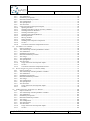

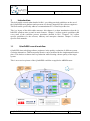

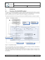


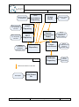
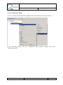
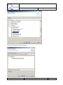
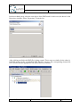

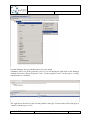


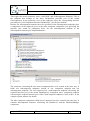
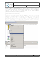


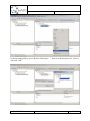


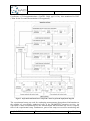


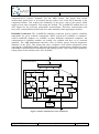


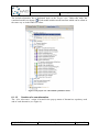
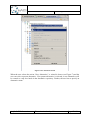
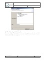
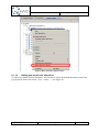
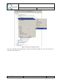
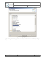
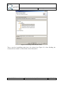

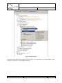


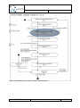

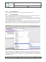
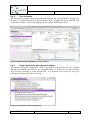
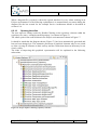
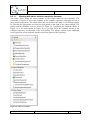


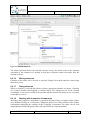


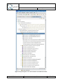


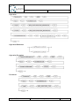


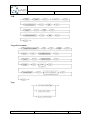


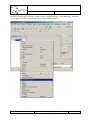

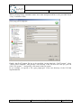
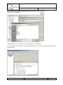
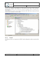


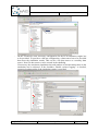
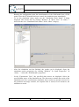
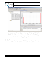


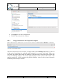
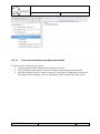


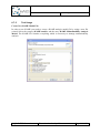
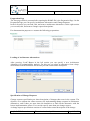
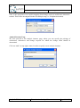

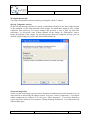
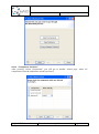
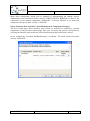
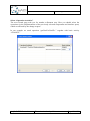
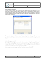
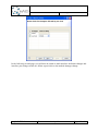

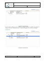
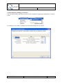
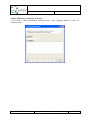

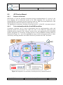
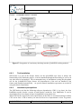


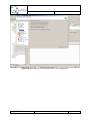


![T9000E [obsolete]](http://vs1.manualzilla.com/store/data/005920932_1-890f13b4deb2f1c3de1d3a852a7c64ca-150x150.png)