Download CMPE 490/450 DESIGN PROJECT UAV Imaging

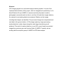
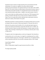
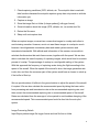
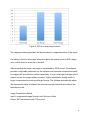
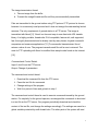
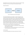
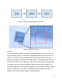
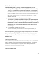
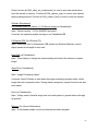
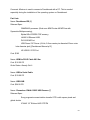
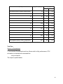
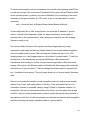
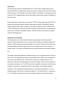
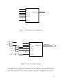
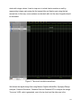
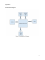
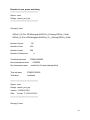
CMPE 490/450 DESIGN PROJECT
UAV Imaging
Shen Yue
[email protected]
Yushi Wang
[email protected]
Yubing Xu
[email protected]
Summary
UAV imaging is a project to process image for UAARG to identify markers on the
ground. Processed images are sent back.
Abstract
UAV Imaging project is an on-board image processing system. It is part of the
Unpiloted Aerial Vehicle (UAV) project, which is designed and operated by U of A
Aerial Robotics Group (UAARG). A camera carried by the plane is used to
photograph a research area from the air, and then full resolution images taken by
the camera for contrasting objects are analyzed. Markers on the images
including their shapes are identified. The processed images are compressed and
sent back to the ground station. [1] The image capturing, image processing,
marker detection, maker shape recognition and image transferring are all
achieved. The result of marker detection is over 90% correct based on provided
images from previous year and from test flight of UAARG. Currently, we are
working with the autopilot group of UAARG on GPS data analysis.
Table of Content
Functional Requirements ................................................................................................. 1
Additional Feature ........................................................................................................ 1!
Future Work .................................................................................................................. 1!
Design and Description of Operation ............................................................................... 2!
Software Structure ........................................................................................................ 2!
Image Capturing Details ........................................................................................... 3!
Image Processing Details ......................................................................................... 4
Image Transmission Details ..................................................................................... 6
Command Control Details ........................................................................................ 7
Recognition Algorithm .............................................................................................. 8
Location Algorithm .................................................................................................... 8
Marker Recognition ................................................................................................ 12
Performance of Software ........................................................................................ 13
Hardware Control ....................................................................................................... 14
Software Requirement ................................................................................................ 15!
Part Lists ........................................................................................................................ 16!
All IO signals .................................................................................................................. 17!
I/O Interfaces .............................................................................................................. 17!
Power supplies ........................................................................................................... 17
Datasheet ...................................................................................................................... 17!
Test plan ........................................................................................................................ 18!
Ubuntu on Pandaboard .............................................................................................. 18!
Chameleon Camera ................................................................................................... 19
The Entire System ...................................................................................................... 19
Test Result ..................................................................................................................... 21!
Integrated Circuit Design ............................................................................................... 21!
References .................................................................................................................... 25!
Appendices .................................................................................................................... 27!
Functional Requirements
There are mainly three functions – image capturing, processing, and transferring in our
project. In image capturing, an onboard camera is adjusted to fast shutter speed and
controlled to sufficiently take full resolution high quality images (1296 * 964 1.2M image)
of the entire search area. After taking the image, our image processing system scans
and analyzes the image to locate the marker and then the image is transferred from raw
data format (pgm) to compressed data format (jpg) with the same resolution but
different quality (based on the transfer rate, the size of the image ranges from 30k to
250k). Once the image is analyzed and compressed, it is transferred to the ground
station using FTP protocol through WiFi.
Our design meets all these three functions. The fastest capturing rate is found to be 6.8
FPS and the maximum transmission rate is 5 FPS. The accuracy of our image
processing is over 90%.
Additional Feature:
Marker Shape Recognition: Markers on the ground have different shapes and colors. In
previous years competitions, they were recognized by human eyes after images were
sent back to ground station. Therefore, the new feature that has been added to our
project is to do this automatically on-board by the embedded system.
Future Work:
Character Recognition: There is an English letter in the middle of each marker, and it
need to be reported in the competition. Like maker shapes, human eyes did this in
previous years. This could be added to the embedded system in the future.
Better algorithm: we can further optimize our algorithm as much as possible in terms of
speed and accuracy.
1
Other features can be added: interpolating GPS and obtain direction information;
providing a 9600 bps tunnel through the processor and WiFi to serial port on ground
station; adapting ground station software for a new way of operating.
Design and Description of Operation
Software Structure
*Icons for camera, folder, and WiFi are taken from the Internet [16, 17, 18]
Figure 1. Block diagram of software design
The overall software design consists of 4 components: image capturing system, image
processing system, image transmission system and command system. Image capturing
serves as the producer of image processing. Image processing is the consumer of
image capturing and the producer of image transmission at the same time. Image
2
transmission is the consumer of image processing. Due to the producer/consumer
relationships of the system, we implement the system with the standard
producer/consumer architecture. We implement each part of the relation with a POSIX
thread [10]. We use two folders as buffers between each producer/consumer relation to
deal with short-term speed mismatch. Two semaphores are used for full and empty to
control data flow between each relation. In addition, two mutual exclusion locks are
used to protect data from multiple accesses at the same time. With this approach, the
producer is blocked if the buffer is full, and the consumer is blocked if the buffer is
empty. There is no empty while-condition-checking loop to waste system resources,
which can be used by other threads of the system.
With different methods of accessing the buffer, the software provides options to process
and transmit either most recent or least recent image first. It also gives the option to
either block the producer when the buffer is full or drop the least wanted (oppose to
priority of processing and transmission) image when the buffer is full. In addition, the
software provides an option to prioritize the transmission of marker images over other
images. After processing or transmitting a file, the software provides an option to keep
or delete the file.
The pseudo code for the implementation can be found in Appendix. Note that within a
mutual exclusion lock, only the name of an image file is stored/removed from a buffer,
the actual read/write and process of the image is outside the lock. This approach allows
minimum operations within the lock and avoids unnecessary blocks of other threads.
Image Capturing Details
Input: Camera
Output: A bayer pattern image file in pgm format and a text file to a folder
The image capturing thread
3
1. Check capturing conditions (GPS, altitude, etc. The autopilot date is read with
fake functions because the autopilot capstone group has not provide us with the
information yet)
2. Capture an image
3. Store the image file in a folder (In bayer pattern[], with pgm format)
4. Store information about the image (GPS, altitude, etc.) in another text file
5. Return the file name
6. Sleep until next capture time
When we capture images, we want two consecutive images to overlap each other to
avoid missing a marker. However, we do not want these images to overlap too much
because it would generate unnecessary data and waste system resource and
transmission bandwidth. With altitude and information of the camera, we are able to
calculate the dimension that each frame covers, together with the speed. We are also
able to calculate the exact frequency of capturing images, which would lead to a certain
percent of overlap. The percentage of overlap is a configurable setting of the system.
With this approach the frequency of capturing varies during the flight according to the
speed of the aircraft. When the speed of the aircraft is slow, the image generation rate
is also low; and then the consumer part of the system would have a chance to catch up
if the buffer is filled up.
We can provide status of buffers to the ground station to adjust the speed of the aircraft
if required. We can also calculate the recommended speed by taking the lower value
from processing rate and transmission rate as the recommended capturing rate; and
then convert the recommended capturing rate to recommended speed of the aircraft.
Rates are calculated from the average of a time period to avoid sudden changing of the
recommended speed. This recommended speed could be feed into the auto pilot
system.
Image Processing Details
Input: Bayer pattern image file in pgm format and text file from a folder
4
Output: A compressed image file in jpg format and a text file to a folder
The image capturing thread
1. Take a bayer pattern image file from the buffer
2. Convert the image from bayer pattern to RGB using function provided by
OpenCV
3. Process the image to get information about the marker
4. Store information about the target (GPS, shape, color, etc) in another text file
5. Compress and save the image in jpg format
6. Return the file name
The platform we work on has a dual core processor. Since a single thread is not able to
utilize full power of a dual core processor, we run two separate, identical, and fully
functional copies of the image processing threads on the system. The number of image
processing thread is automatically configured to equal to the number of cores of the
platform; and it can also be set manually. The following chart compares the
performance of a single thread, two threads, and three threads on a dual core system. It
can be observed that, the performance caps when the number of threads equals to the
number of processor cores.
5
Figure 2. FPS on a dual core processor
The image processing algorithms will be discussed in a separate section of this report.
If a marker is found in the image, information about the marker, such as GPS, shape,
color, will be stored in a text file on the disk.
After processing the image, the image is compressed to JPEG format. The software
provides configurable parameters for the minimum and maximum compression quality
for images with and without a marker respectively. It is set to be high for images with a
marker and low for images without a marker. Higher compression quality results in
longer compression time and much larger file size. The software automatically adjust
the compression ratios in between the minimum and the maximum according to the
transmission rate.
Image Transmission Details
Input: A compressed image file and a text file from a folder
Output: WiFi transmission with FTP protocol
6
The image transmission thread
1. Take an image from the buffer
2. Transmit the image file and text file until they are successfully transmitted
Files are transmitted to the ground station using FTP protocol. FTP protocol is chosen
because it is a commonly used protocol and it does not encrypt the data wasting limited
resource. The only requirement of ground station is a FTP server. The image is
transmitted with libcurl[11]. “libcurl is a free and easy-to-use client-side URL transfer
library. It is highly portable, thread-safe, IPv6 compatible, feature rich, well supported,
fast, thoroughly documented and is already used by many known, big and successful
companies and numerous applications.”[11] For successful transmissions, libcurl
returns a value of zero. The program transmits each file until a zero is returned. The
code for FTP uploading with libcurl is modified from sample code found on the Internet
[15].
Command and Control Details
Input: A text file on the FTP server
Output: Change of parameters
The command and control thread
1. Download the command file from the FTP server
2. Parse the text file for commands
3. Change settings of the program
4. Wait for a period of time and go back to step 1.
The command and control thread is used to execute commands issued by the ground
station. For simplicity for the ground operator, we designed the commands to be stored
in a text file on the FTP server. Our program periodically download and check the
content of the text file, and change the settings accordingly. The settings are saved in a
global variable protected by multi-thread locks. The other parts of the system will read
7
the parameters for every new image. Currently we only have the command to change
shutter speed. However, other commands can be easily added if needed.
Recognition Algorithm
Figure 3. Relationship of location and recognition
The recognition algorithm has two main stages – location and recognition. In the
location stage, the program finds the marker on the image, and finds all pixels that
belong to the marker. This information is stored on another black and white picture with
black representing the background, and white representing the marker. The size of this
image is just enough to enclose the marker. After that, the black and white image along
with the original image is passed to the recognition stage. The recognition stage
identifies the shape from the black and white image, and uses the black and white
image as a mask on the original image to mask off the ground, and then identifies more
information about the marker. Benefits from this implementation are:
● Isolation of location from recognition: an implementation change of one stage
does not affect the other stage.
● Save system resources: instead of the whole image, the recognition stage only
process the data output from the location stage.
Location Algorithm
The marker locating algorithm has three steps as shown below in Figure 4.
8
Figure 4. Marker locating algorithm flow chart
Figure 5. Example of a grid
Overview
The marker locating algorithm is based on a grid system (shown in Figure 5). The red
square represents a grid. It is divided into 8 segments separated by the black dots on
the picture. The size of the grid is calculated from the pixel-per-meter of the image
based on the height and tilt at which the image is taken. The next grid always starts at
the middle of the previous grid. Basically, in the first step, the algorithm calculates data
for the grid; in the second step the algorithm finds grids that contains an edge; in the
last step, the algorithm connects nearby edge-grids to form a shape, and performs basic
check on the dimension of the shape. If the shape passes the basic check then it is
passed to the marker recognition stage for further operations.
9
Grid Data Calculation Detail
Data of each grid is stored in a c struct. The main components of the struct are:
●
An array of 8 cvScalar[1] (a cvScalar is an array of 3 int, used to store a color)
The array of 8 cvScalar stores the mean color of each edge. For example, the
first cvScalar of the array stores the mean color of the two segments at the top,
the second cvScalar stores the mean color of the two segments near the upper
right corner, the third cvScalar of the array stores the mean color of the two
segments on the right.
●
An int stores the orientation of the edge contained in the grid
The orientation of the edge is calculated by comparing each opposite edges like
edge0 and edge 4 (top edge, bottom edge), edge1 and edge4 (upper right edge,
lower left edge). The pair of edges with the most color difference is calculated as
the edge in the grid, and the orientation value is the smaller value of the two
opposite edges.
●
A cvScalar stores the mean color of the grid
The mean color of the grid is calculated from all the edges around the grid.
All the colors above are stored in LAB color space converted from RGB [24]. Lab color
space is used because Delta E [25]. The color difference of two colors is calculated
using the Lab color space. The code for color conversion and delta E calculation is in
application notes.
Edge Grid Identification Detail
Using the Data calculated from the previous step, we are able to find all the grids with
edges of the image. This is done by setting a threshold delta E value. If the opposite
edge pair with the most difference in a grid has a delta E value greater than the
threshold, the grid is identified as a grid with edge.
Edge Grid Connection Detail
10
For each grid with edges (edge-grids), we check all the nearby edge-grids. If the most
difference edge pair on the current edge-grid has the same color as the nearby edgegrid, then we connect the nearby grid with the current grid. The color check is to ensure
we do not connect the edge of different object together. This connection is done by
setting a one on a 2-D array. After connecting all the edges, we check the dimension of
the connected region. If it passes the dimension check, the 2D array representing the
shape of the object is sent to the marker recognition stage for further process and
verification.
Properties of the Locating algorithm
Our locating algorithm is extremely fast because of the following reasons:
●
Instead of assessing the whole image, it only assesses the pixels on the square,
which reduces the amount of data to process.
●
To calculate the mean of each edge, we first calculate the mean of each of the 8
segments on the square, and then we use the mean of the 2 segments to
calculate the mean of the edges. The mean of the whole grid is calculated with
the mean of 4 edges. Therefore, no extra calculation is performed.
●
Instead of converting the whole image at the beginning, the RGB->LAB
conversion is done after calculating the mean of each segments, this approach
saves a lot of CPU power for color conversion.
●
The rest of the operations are done on the grids, without accessing the original
image. At cruising altitude, the size of each grid will be around 30x30. Which
means there are 900 times less grids than the number of pixels of the original
image.
Our locating algorithm has high tolerance to blurry pictures:
It does not require sharp edges to work because the edge of an object will be identified
as long as there is enough difference over the length of a grid. This is important
because our system will be used on the aircraft. We expect the plane to be unstable at
some period of the flight which resulting in blurry pictures. Furthermore, our camera
11
works on a fixed focal length. If the aircraft is flying too high or too low, the picture will
be blurry.
Marker Recognition
Currently we are able to identify the shape of a marker. It is done by calculate the
following properties of the shape that is stored in the black and white image.
●
hu1
●
hu2
●
hu3
●
number of edge
●
ratio of the longest edge to the shortest edge
All of these properties are independent of orientation, and size of the shape. For each
shape, we calculate a loose range of each property to make sure a property of an input
always falls into the range of the corresponding shape. With all five properties, we are
able to identify a shape.
The following steps are taken for a given input:
1.
Add all shapes as possible shapes to a queue
2. Calculate a property of the input
3. If range of the property of a possible shape in the queue disagrees with the
property of the input, remove the possible shape from the queue
4. If there is more than 1 possible shape in the queue, go back to step 2 with
another property
Following is the detailed description for each property.
HU
“Hu set of invariant moments are invariant under translation, changes in scale, and also
rotation. [12] (The calculation of Hu moments can be found in the reference)” We are
only using the first 3 of the 7 hus, because the other 4 hus does not differentiate such
12
simple shapes. As our shape is too simple, the first three hus does not differentiate all
the shapes and we have to use other properties in addition to hus.
Number of edges
The edges are approximated form the black and white image using OpenCV [13]
providing function cvApproxPoly [14]. This function “approximates polygonal curve(s)
with the specified precision. [14]” The function not only calculates the number of edges,
but also eliminates effect of imperfections on the edges or corners of the shape from the
black and white image; however, this function cannot recognize curves, it approximates
curves with polygonal curves. With our current parameters, a circle is approximated with
7 or 8 edges. With the Hu and number of edges, we are still not able to differentiate
between all shapes, more properties needs to be used.
Edge Ratio
With OpenCV [13] functions, we are able to calculate the length of each edge
approximated by cvApproxPoly [14]. Using the ratio of the longest edge to the shortest
edge, along with other properties, we are able to identify all the shapes.
Performance of the Software
The software is targeted for real-time process on a system with limited resources.
Performance of the algorithm and implementation is critical to the system. The following
things are done to ensure our software meets the performance requirement.
●
Two separate FPS meter are implemented for both processing and transmission
component to closely monitor the performance of the software as we develop it.
●
Code within critical loops is carefully optimized.
●
The time cost of each OpenCV[13] provided function is checked before it is used.
●
Replacing pixel accessing function provided by OpenCV[13] with direct pointer
accessing for better performance.
●
No busy while loop for condition checking. Everything is done with semaphores
and timed sleep.
●
Use of multi-thread to take advantage of multi-core.
13
●
Use of custom designed and optimized algorithms for our particular task.
●
Use of multi-stage operations with faster stage before slower stage, to reduce
data processed in the slower stage.
●
Constant check to eliminate memory leak.
●
Many optimizations based on the data from the autopilot.
●
Use of three different implementation of queues (interchangeable but inefficient
in terms of system resource) for different situation
Hardware Control
In order to obtain images in a high capturing rate, a C library called libdc1394 is
introduced. Function dc1394_camera_new() is used to initialize the camera, and
function dc1394_feature_set_mode() is used to set the camera. Function
dc1394_feature_set_mode() has three parameters, where the first one is the camera
number, the second and third ones are the setting term and the setting value. For
example when we call dc1394_feature_set_mode (camera,
DC1394_FEATURE_SHUTTER, DC1394_FEATURE_MODE_MANUAL), it means
changing the shutter setting of the camera into manual mode. Then we can change the
shutter speed of the camera by calling dc1394_feature_set_value(camera,
DC1394_FEATURE_SHUTTER, 100) (Here we change it into 100). The value of the
shutter speed ranges from 1 to 1007, where 1 is the darkest and 1007 is the brightest.
Based on our test, 100 is the best value for our project.
Function dc1394_capture_dequeue() is used to setup the image buffer for capturing an
image, and the capture policy is waiting or polling. Dc1394_capture_enqueue() is used
to read the image from the camera. Both functions are used together and sequentially to
capture the image.
To store the image, first we need to use function
dc1394_get_image_size_from_video_mode() to get the image size, and then use
function fwrite() to write the image to a file with size specified by the third parameter.
14
At last, function dc1394_video_set_transmission() is used to stop data transmission
from the camera to memory. Function dc1394_capture_stop() is used to stop camera
keeping taking pictures. Function dc1394_camera_free() is used to close the camera.
Software Requirement
Pre-installed OMAP3/4 Oneiric (11.10) Server Image (on Pandaboard)
Spec: “Ubuntu version 11.10 for OMAP3/4 processor”
Comment: the operating system running on our Pandaboard ES
FlyCapture SDK (On Windows PC)
Spec: “Driver with GUI for Chameleon USB camera on Windows Machine, used to
adjust camera focal length for test uses”
libdc1394 (on Pandaboard)
Spec: ”Driver library to change the camera setting and control the camera to capture
image”
OpenCV(on Pandaboard)
Spec: “Image Processing Library”
Comment: OpenCV library is used when the image processing program reads, writes
image files and compresses them. During marker recognition, several functions are also
been called.
Libcrl (on Pandaboard)
Spec: “Library used to transfer image from on board system to ground stations through
ftp protocol”
Minicom (On Ubuntu Workstation)
Spec: “A test-based modem control and terminal emulation program”
15
Comment: Minicom is used to connect a Pandaboard with a PC. This is needed
especially during the installation of the operating system on Pandaboard.
Part Lists
Name: Pandaboard ES [6]
Relevant Spec:
OMAP4460 processor (Dual-core ARM Cortex-A9 MPCore with
Symmetric Multiprocessing),
Elpida 8Gb LPDDR2 POP memory,
LAN9514 Ethernet HUB,
DVI-D/HDMI Port.
USB Power/ DC Power (+5Vdc, 2.0mm center pin diameter/6.5mm outer
hole diameter jack) [Pandaboard Manual p13]
HS USB 2.0 OTG Port
Cost: $182
Name: HDMI to DVI-D Cable 6ft/1.8m
Cost: $ 26.00 CD
Order Status: Already Got It
Name: USB to Serial Cable
Cost: $ 29.99 CD
Name: USB HUB
Cost: $24.99 CD
Name: Chameleon CMLN-13S2C USB Camera [7]
Relevant Spec:
Sony progressive scan interline transfer CCD’s with square pixels and
global shutter
ICX445 1/3” EXview HAD CCDTM
16
1296(H) x 964(V) max resolution
Cost: N/A
Name: FUJINON 1:1.4/12.5mm HF12.5HA-1B Lens [8]
Relevant Spec:
2/3-Inch CCD Imager size
12.5mm focus length
f/1.4 to f/16 Aperture
Manual iris
Manual focus
Cost: N/A
All IO signals
I/O Interfaces
GPS: RS-232 level 4800b/s serial
Network: 10/100 Ethernet, WiFi
Camera: USB 2.0 (Pin 1: +5V, Pin 2: Data-, Pin 3: Data+, Pin4: Ground)
Power supplies
Camera: USB
Altera DE2: 9V AC/DC adaptor
Pandaboard: 5V DC power
Datasheet
The following table shows the image transferring data:
17
Quality(
Image(Size((KByte)(
Image(s)/s(
(
(
5Mbit/s( 1Mbit/s(
0"(Lowest"Quality;"Greatest"Compression)"
23"
27.2"
5.4"
10"
43"
14.5"
2.9"
20"
67"
9.3"
1.9"
30"
87"
7.2"
1.4"
40"
103"
6.1"
1.2"
50"
120"
5.2"
1.0"
60"
138"
4.5"
0.9"
70"
167"
3.7"
0.7"
80"
217"
2.9"
0.6"
90"
333"
1.9"
0.4"
95"
484"
1.3"
0.3"
97"
611"
1.0"
0.2"
967"
0.6"
0.1"
100"(Highest"Quality;"Least"Compression)"
Table1. Image Transmission
Test Plan
Ubuntu on Pandaboard
To test whether Pandaboard could run Ubuntu with its fully performance, CPU
information is checked with command line:
cat /proc/cpuinfo
The output is pasted below:
18
Figure 6. Test Output of Pandaboard running Ubuntu
From the above, we can tell there are two working processors – processor 0 and 1. The
speed of each one is about 1.2GHz, which matches what Pandaboard user’s manual’s
specification. The dual-core OMAP A9 CPU can fully operates with Ubuntu running on
it. Therefore, we can use Ubuntu Oneiric as the operating system of software
environment for UAV Imaging project.
Chameleon Camera
Chameleon camera is tested on a PC running Ubuntu first, and then it is moved to
Pandaboard. The official driver with a GUI for Windows 7 is provided by Point Gray. The
manufacture of Chameleon Camera is called FlyCap2. With FlyCap2, Chameleon
Camera captures image in real time, such that we can use FlyCap2 to adjust the setting
of the camera easily. However, when it moves to Ubuntu, two differences show up:
Ubuntu version does not have a GUI; and the frame capturing rate is low (2 to 3 FPS on
Pandaboard). Therefore, we choose another camera control library called libdc1394.
With this one, the image capturing rate can reach 5 FPS and the camera can be set by
calling several function from libdc1394. (As discussed in “Camera Control” session)
The Entire System
19
To test the entire system, we use a wireless router to build a local network with WiFi as
our test environment. We connect the Pandaboard to the router with an Ethernet cable
as the onboard system (on plane), and use my MacBook Pro connecting to the router
wirelessly as the ground station. An FTP server is set on “ground station” by using
command:
sudo -s launchctl load -w/System/Library/LaunchDaemons/ftp.plist
In the configuration file of UAV Image System, we setup the IP address of “ground
station”, the path of the destination folder for image transferring, and the path of
command file on the “ground station”. After setting up everything, the UAV Imaging
System is ready to use.
First, we test basic functions of the system, including image capturing, image
compression and image transferring. (Marker detection and marker shape recognition
are not included at this moment) After boosting the Pandaboard, we run our UAV
Imaging system on it, and images show up in the folder of “ground station”. To test the
reconnection of the transferring, we unplug the Ethernet cable connected to
Pandaboard. After waiting for a while, the processed image buffer is filled with some
images. We re-plug in the Ethernet cable on Pandaboard. New images with smaller file
size show up on “ground station”. Then we change the shutter speed in command file
into 1 (smallest shutter speed). The next image shown up on “ground station” becomes
dark.
Second, we simulate the situation of real competition indoor by making some smaller
marker (3cm x 3cm), and locating them on the floor. Then we readjust the focus of
Chameleon Camera to a suitable value by using FlyCap2 on Windows machine. (In
competition, the focus of camera should be set to infinity, since the plane flies as high
as 200 ft.) As soon as the system starts, a person carries the camera taking pictures of
the markers on the floor. At last we compare and calculate the detection and recognition
result by observing the images transferred back to “ground station”.
20
Test Result
The average test result on Pandaboard ES is 2.3 FPS without image capturing and
image transmission. Comparing to image processing, capturing and transmission takes
much less time of CPU (based on the tests on Mac). We achieve our design goal, which
is about 2 FPS. Integrated tests with all three parts combined are going to be applied in
the near future.
By the submission of this report, we achieve 7 FPS for image capturing, and 5 FPS for
image processing with marker detection and shape recognition. Meanwhile, without
marker detection and shape recognition, the image compression can be as fast as 8 10 FPS. Although we cannot test the data transferring rate practically, we calculate the
result, and it is shown in datasheet session. Overall, the test result shows our system
achieves the design goal.
Integrated circuit design
The integrated circuit only included the basic image analysis that finds potential
markers. Actual images taken from a camera are not used since sending images from
camera to DE2 and processing them requires a lot of work. The input to be used is the
processed black and white image, which is from computer point of view, a bunch of
number points. The output is whether there is a potential marker in the specific search
box.
The design follows the algorithm in software design, but it is implemented into VHDL so
that “a set of test benches can then be constructed and the VHDL can be simulated to
verify the correct behavior” [2]. A search box is used to go through all points. The
dimension of the box is determined by the size of the target. We can use 4×4 (which is
now used in software) or 3×3 in VHDL and set the variable in software in with the same
number for comparison. Signals are used to store values and calculate standard
deviations. If the calculated standard deviation is less than the threshold (i.e., 0.8 in
software design), then there is a potential marker (i.e., the output will be 1, otherwise it
is 0). We build a 4×4 search box and its schematic is shown in the following figure:
21
clk
rst
Marker(0/1)
a[7…0]
b[7…0]
c[7…0]
p[7…0]
Figure 7. The schematic of 4×4 search box
clk
clk
rst
rst
p0[7…0]
a[7…0]
p1[7…0]
b[7…0]
p2[7…0]
c[7…0]
p15[7…0]
p[7…0]
Marker (0/1)
Marker(0/1)
Figure 8. Top-level hardware diagram
A testbench for the VHDL code is created to verify the design. The simulated result is in
Figure 9. It shows the result is correct; however, the result is not precise since it only
22
deals with integer values. It can be improve to include fraction number as well by
representing integer parts using the first several bits and fraction part using the last
several bits. In this way, more numbers can be dealt with, but the size of signals should
be increased.
Figure 9. The circuit simulation waveforms
We follows the digital design flow using Mentor Graphics ModelSim, Synopsys Design
Analyzer, Cadence Encounter, Cadence Diva and Cadence DFII to analyze the design.
Tow more VHDL code is generated, one is the top level and the other one is the
23
testbench for the top level. In Synopsys Design Analyzer, several reports are generated
and attached in appendix. After the gate-level simulation, the layout of the chip is
generated using Cadence Encounter. Finally the Cadence DFII is used to find out the
LVS clean design.
We found that ASIC is the fastest and software is the slowest as expected. The time is
shown in the following table. There are some still some tradeoffs in design time,
manufacturing time, capital cost, volume cost, speed, power, area, etc. need to be
considered. Therefore, even the speed of the ASIC is the fastest; software design is
more suitable to our project.
Design Method
Time (s)/ Frame
Software
5
FPGA
0.076
ASIC
0.0176
Table 2. Timing Comparison
24
References:
[1] “OpenCV.” Internet: http://opencv.willowgarage.com/wiki/, August 24, 2011 [January
20, 2012].
[2] Neil H. E. Weste and David Money Harris. CMOS VLSI Design: A Circuits and
Systems Perspective. US: Pearson Education, 2009, pp. 637 - 641, 681.
[3] Elham Ashari and Richard Hornsey. “FPGA Implementation of Real-Time Adaptive
Image Thresholding.” [On-line]. pp. 1. Available:
http://www.cse.yorku.ca/visor/pdf/PN04_Adaptive_thresh.pdf [ Feb 4, 2012].
[4] Abdul Manan. “Implementation of Image Processing Algorithm on FPGA.” Akgec
Journal of Technology. [On-line]. Vol.2, No.1 pp. 27-28.
[5] “BeagleBoard-xM Reference Manual” Internet:
http://beagleboard.org/static/BBxMSRM_latest.pdf, April 4, 2010 [January 20, 2012].
[6] “Pandaboard ES User Reference Manual” Internet:
http://pandaboard.org/sites/default/files/board_reference/ES/Panda_Board_Spec_DOC21054_REV0_1.pdf, September 29, 2011 [January 20, 2012].
[7] “Chameleon CMLN-13S2C USB Camera” Internet:
http://www.ptgrey.com/products/chameleon/Chameleon_datasheet.pdf, [January 20,
2012]
[8] “FlyCapture SDK” Internet:
http://www.ptgrey.com/support/downloads/documents/Chameleon%20Getting%20Start
ed%20Manual.pdf, [January 20, 2012]
[9] “ Introduction to the Altera SOPC Builder Using VHDL Design.” Internet:
ftp://ftp.altera.com/up/pub/Tutorials/DE2/Computer_Organization/tut_sopc_introduction_
vhdl.pdf, [Feb 4, 2012].
[10] “POSIX Threads Programming” Internet:
https://computing.llnl.gov/tutorials/pthreads/, [March 8, 2012]
[11] “libcurl - the multiprotocol file transfer library”
Internet: http://curl.haxx.se/libcurl/, [March 8, 2012]
[12] Image moment
Internet: http://en.wikipedia.org/wiki/Image_moment, [March 8, 2012]
[13] “OpenCV” Internet: http://opencv.willowgarage.com/wiki/, [April 17, 2012]
25
[14] “Structural Analysis and Shape Descriptors”
Internet:
http://opencv.willowgarage.com/documentation/structural_analysis_and_shape_descript
ors.html, [March 8, 2012]
[15] “LIBCURL
FTP
To realize the upload and download
fucntionality using Libcurl”, Internet:
http://blog.csdn.net/vipfengxiao/article/details/6027742, [March 8, 2012]
[16] http://www.whatthetech.com/blog/wp-content/uploads/2010/08/leopard-folder.png
[17] http://www.ptgrey.com/products/chameleon/images/Chameleon_1024px.jpg
[18] http://www.thetelecomblog.com/wp-content/uploads/2011/11/wifi-logo.gif
[19] “FUJINON 1:1.4/12.5mm HF12.5HA-1B Lens” Internet:
http://www.bhphotovideo.com/c/product/404246REG/Fujinon_HF125HA1B_HF12_5HA_1B_12_5_mm_F1_4.html, [Mar 7, 2012]
[20] Pingjim Wei, Liang Zhang, Changzheng Ma and Tat Soon Yeo. “Fast Median
Filtering Algorithm Based on FPGA,” in Signal Processing (ICSP), 2010 IEEE 10th
International Conference, pp. 426-429.
[21] “Install,” Internet:
https://wiki.ubuntu.com/ARM/Server/Install?action=show&redirect=ARM%2FOMAPHea
dlessInstall [March 8, 2012]
[22] “Minicom,” Internet:http://en.wikipedia.org/wiki/Minicom [March 8, 2012]
[23] “Bayer filter,” Internet: http://en.wikipedia.org/wiki/Bayer_filter [April 16, 2012]
[24] “Lab color space”, Internet: http://en.wikipedia.org/wiki/Lab_color_space [April 16,
2012]
[25] “Delta E: The Color Difference”, Internet:
http://www.colorwiki.com/wiki/Delta_E:_The_Color_Difference [April 16, 2012]
[26]“libdc1394” Internet: http://damien.douxchamps.net/ieee1394/libdc1394/ [April 17,
2012]
[27] “libcurl – the multiprotocol file transfer library” Internet: http://curl.haxx.se/libcurl/
[April 17, 2012]
26
Appendices
Hardware Block Diagram
Figure1. Hardware Block Diagram
27
Pseudo code for thread implementation
imageCapturingThread
{
wait(unprocessedImageBufferEmpty);
fileName=captureImage();
lock(&captureLock);
addFileNameToUnprocessedImageBuffer(fileName);
unlock(&captureLock);
post(unprocessedImageBufferFull);
}
imageProcessingThread
{
post(unprocessedImageBufferFull);
wait(processedImageBufferEmpty);
lock(&captureLock);
fileName=removeFileNameFromUnprocessedImageBuffer();
unlock(&captureLock);
processImage(fileName);
lock(&processLock);
addFileNameToProcessedImageBuffer(fileName);
unlock(&processLock);
post(processedImageBufferFull);
wait(unprocessedImageBufferEmpty);
28
}
imageTransmissionThread
{
post(processedImageBufferFull);
lock(&processLock);
fileName=removeFileNameFromUnprocessedImageBuffer();
unlock(&processLock);
transmitImage(fileName);
wait(processedImageBufferEmpty);
}
29
Reports for area, power and timing
****************************************
Report : area
Design : search_box_top
****************************************
Library(s) Used:
GSCLib_2.0 (File: /EDA/kits/gpdk18/GSCLib_3.0/timing/GSCLib_3.0.db)
GSCLib_IO (File: /EDA/kits/gpdk18/GSCLib_IO_1.4/timing/GSCLib_IO.db)
Number of ports:
138
Number of nets:
405
Number of cells:
268
Number of references:
Combinational area:
4
3726000.000000
Noncombinational area:
Net Interconnect area:
0.000000
undefined (No wire load specified)
Total cell area:
3726000.000000
Total area:
undefined
****************************************
Report : area
Design : search_box_top
Version: Y-2006.06-SP4
Date : Tue Apr 17 16:53:02 2012
****************************************
Library(s) Used:
30
GSCLib_2.0 (File: /EDA/kits/gpdk18/GSCLib_3.0/timing/GSCLib_3.0.db)
GSCLib_IO (File: /EDA/kits/gpdk18/GSCLib_IO_1.4/timing/GSCLib_IO.db)
Number of ports:
138
Number of nets:
405
Number of cells:
268
Number of references:
Combinational area:
4
3726000.000000
Noncombinational area:
Net Interconnect area:
0.000000
undefined (No wire load specified)
Total cell area:
3726000.000000
Total area:
undefined
****************************************
Report : power
-analysis_effort low
Design : search_box_top
****************************************
Library(s) Used:
GSCLib_2.0 (File: /EDA/kits/gpdk18/GSCLib_3.0/timing/GSCLib_3.0.db)
GSCLib_IO (File: /EDA/kits/gpdk18/GSCLib_IO_1.4/timing/GSCLib_IO.db)
Operating Conditions: typical Library: GSCLib_2.0
Wire Load Model Mode: top
31
Global Operating Voltage = 3
Power-specific unit information :
Voltage Units = 1V
Capacitance Units = 1.000000pf
Time Units = 1ns
Dynamic Power Units = 1mW
(derived from V,C,T units)
Leakage Power Units = 1nW
Cell Internal Power = 319.7285 mW (96%)
Net Switching Power = 12.6946 mW
(4%)
--------Total Dynamic Power
= 332.4232 mW (100%)
Cell Leakage Power
= 6.5710 mW
Loading db file '/EDA/kits/gpdk18/GSCLib_3.0/timing/GSCLib_3.0.db'
Loading db file '/EDA/kits/gpdk18/GSCLib_IO_1.4/timing/GSCLib_IO.db'
Information: Propagating switching activity (low effort zero delay simulation). (PWR-6)
Warning: Design has unannotated primary inputs. (PWR-414)
Warning: Design has unannotated sequential cell outputs. (PWR-415)
****************************************
Report : power
-analysis_effort low
Design : search_box_top
Version: Y-2006.06-SP4
Date : Tue Apr 17 16:53:15 2012
****************************************
32
Library(s) Used:
GSCLib_2.0 (File: /EDA/kits/gpdk18/GSCLib_3.0/timing/GSCLib_3.0.db)
GSCLib_IO (File: /EDA/kits/gpdk18/GSCLib_IO_1.4/timing/GSCLib_IO.db)
Operating Conditions: typical Library: GSCLib_2.0
Wire Load Model Mode: top
Global Operating Voltage = 3
Power-specific unit information :
Voltage Units = 1V
Capacitance Units = 1.000000pf
Time Units = 1ns
Dynamic Power Units = 1mW
(derived from V,C,T units)
Leakage Power Units = 1nW
Cell Internal Power = 10.3676 mW (96%)
Net Switching Power = 410.6353 uW
(4%)
--------Total Dynamic Power
= 10.7782 mW (100%)
Cell Leakage Power
= 6.5710 mW
****************************************
Report : timing
-path full
-delay max
33
-max_paths 1
Design : search_box_top
****************************************
Operating Conditions: typical Library: GSCLib_2.0
Wire Load Model Mode: top
Startpoint: coreG/difference_a_reg_1_
(rising edge-triggered flip-flop clocked by padClk)
Endpoint: coreG/sumq_reg_15_
(rising edge-triggered flip-flop clocked by padClk)
Path Group: padClk
Path Type: max
Point
Incr
Path
-------------------------------------------------------------------------clock padClk (rise edge)
0.00
0.00
clock network delay (ideal)
0.00
0.00
coreG/difference_a_reg_1_/CK (SDFFSRX1)
0.00
coreG/difference_a_reg_1_/Q (SDFFSRX1)
coreG/U35/Y (BUFX3)
0.00 r
0.31
0.42
0.31 r
0.73 r
coreG/mult_129_14/A_1_ (search_box_DW02_mult_2)
0.00
coreG/mult_129_14/U52/Y (AND2X1)
0.14
0.87 r
coreG/mult_129_14/U31/Y (XOR2X1)
0.09
0.96 f
coreG/mult_129_14/S2_2_5/S (ADDFX1)
0.16
1.12 r
coreG/mult_129_14/S2_3_4/S (ADDFX1)
0.16
1.28 r
coreG/mult_129_14/S2_4_3/S (ADDFX1)
0.16
1.43 r
coreG/mult_129_14/S2_5_2/S (ADDFX1)
0.16
1.59 r
coreG/mult_129_14/S2_6_1/S (ADDFX1)
0.16
1.75 r
coreG/mult_129_14/S4_0/S (ADDFX1)
0.16
0.73 r
1.91 f
coreG/mult_129_14/FS_1/A_5_ (search_box_DW01_add_17)
0.00
1.91 f
coreG/mult_129_14/FS_1/SUM_5_ (search_box_DW01_add_17)
0.00
1.91 f
34
coreG/mult_129_14/PRODUCT_7_ (search_box_DW02_mult_2)
0.00
1.91 f
coreG/add_8_root_add_0_root_add_129_15/B_7_ (search_box_DW01_add_3)
0.00
1.91 f
coreG/add_8_root_add_0_root_add_129_15/U1_7/CO (ADDFX1)
0.13
2.05 f
coreG/add_8_root_add_0_root_add_129_15/U1_8/CO (ADDFX1)
0.12
2.17 f
coreG/add_8_root_add_0_root_add_129_15/U1_9/CO (ADDFX1)
0.12
2.29 f
coreG/add_8_root_add_0_root_add_129_15/U1_10/CO (ADDFX1)
0.12
2.42 f
coreG/add_8_root_add_0_root_add_129_15/U1_11/CO (ADDFX1)
0.12
2.54 f
coreG/add_8_root_add_0_root_add_129_15/U1_12/S (ADDFX1)
0.16
2.70 f
coreG/add_8_root_add_0_root_add_129_15/SUM_12_ (search_box_DW01_add_3)
0.00
2.70 f
coreG/add_5_root_add_0_root_add_129_15/B_12_ (search_box_DW01_add_2)
0.00
2.70 f
coreG/add_5_root_add_0_root_add_129_15/U1_12/CO (ADDFX1)
0.13
2.84 f
coreG/add_5_root_add_0_root_add_129_15/U1_13/S (ADDFX1)
0.16
3.00 f
coreG/add_5_root_add_0_root_add_129_15/SUM_13_ (search_box_DW01_add_2)
0.00
3.00 f
coreG/add_1_root_add_0_root_add_129_15/B_13_ (search_box_DW01_add_1)
0.00
3.00 f
coreG/add_1_root_add_0_root_add_129_15/U1_13/CO (ADDFX1)
0.13
3.13 f
coreG/add_1_root_add_0_root_add_129_15/U1_14/S (ADDFX1)
35
0.16
3.29 f
coreG/add_1_root_add_0_root_add_129_15/SUM_14_ (search_box_DW01_add_1)
0.00
3.29 f
coreG/add_0_root_add_0_root_add_129_15/B_14_ (search_box_DW01_add_0)
0.00
3.29 f
coreG/add_0_root_add_0_root_add_129_15/U1_14/CO (ADDFX1)
0.13
3.43 f
coreG/add_0_root_add_0_root_add_129_15/U1_15/S (ADDFX1)
0.14
3.57 f
coreG/add_0_root_add_0_root_add_129_15/SUM_15_ (search_box_DW01_add_0)
0.00
3.57 f
coreG/U78/Y (AND2X1)
0.04
3.61 f
coreG/sumq_reg_15_/D (SDFFSRX1)
0.00
data arrival time
clock padClk (rise edge)
clock network delay (ideal)
3.61
185.00
0.00
185.00
185.00
coreG/sumq_reg_15_/CK (SDFFSRX1)
library setup time
data required time
3.61 f
0.00
-0.17
185.00 r
184.83
184.83
-------------------------------------------------------------------------data required time
data arrival time
184.83
-3.61
-------------------------------------------------------------------------slack (MET)
181.22
36
Schematics from Design Analyzer Synopsys
37
Chip Layout from Cadence Encounter
38
Layout from Cadence DFII
39
Source code
Please see the compressed file online
40