1
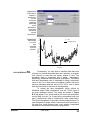
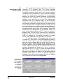
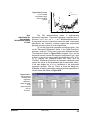
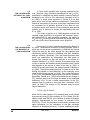
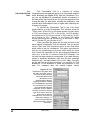
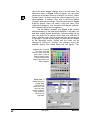
WinBreak
Automated software program for the detection of the gas exchange threshold
Excluded
< Breakpoint
> Breakpoint
40.0
38.0
36.0
34.0
32.0
30.0
6.0
1.0
28.0
26.0
5.0
0.8
24.0
0.6
22.0
4.0
20.0
0.0
5.0
10.0
15.0
20.0
25.0
0.4
Time (min)
3.0
0.2
2.0
0.0
1.0
-0.2
-0.4
0.0
0.0
0.5
1.0
1.5
2.0
2.5
3.0
3.5
4.0
4.5
0.0
5.0
5.0
10.0
15.0
20.0
25.0
Time (min)
VO2 (L/min)
version 3.7
USER
GUIDE
Copyright © 2003
Epistemic Mindworks
All rights reserved
WinBreak
User Guide
1
2
User Guide
WinBreak
Copyright © 2003 EPISTEMIC MINDWORKS. All rights reserved.
WinBreak version 3.7
End-User License Agreement
IMPORTANT - READ CAREFULLY: This End-User License Agreement ("EULA") is a legal agreement between you (either an individual or a single
entity) and EPISTEMIC MINDWORKS for the software product identified above, which includes computer software and may include associated
media, printed materials, and "online" or electronic documentation ("SOFTWARE PRODUCT"). The SOFTWARE PRODUCT also includes any
updates and supplements to the original SOFTWARE PRODUCT provided to you by EPISTEMIC MINDWORKS. Any software provided along with
the SOFTWARE PRODUCT that is associated with a separate end-user license agreement is licensed to you under the terms of that license
agreement. You agree to be bound by the terms of this EULA by installing, copying, downloading, accessing or otherwise using the SOFTWARE
PRODUCT. If you do not agree, do not install or use the SOFTWARE PRODUCT.
Software PRODUCT LICENSE
The SOFTWARE PRODUCT is protected by copyright laws and international copyright treaties, as well as other intellectual property laws and
treaties. The SOFTWARE PRODUCT is licensed, not sold.
1.
2.
GRANT OF LICENSE. EPISTEMIC MINDWORKS grants you the following rights provided that you comply with all the terms and conditions of
this EULA. Installation and use. You may install and use copies of the SOFTWARE PRODUCT on your computer, including a workstation,
terminal or other digital electronic device ("COMPUTER"). Storage/Network Use. You may also store or install a copy of the SOFTWARE
PRODUCT on a storage device, such as a network server.
DESCRIPTION OF OTHER RIGHTS AND LIMITATIONS.
•
•
•
•
•
3.
4.
5.
6.
7.
8.
Limitations on Reverse Engineering, Decompilation, and Disassembly. You may not reverse engineer, decompile, or
disassemble the SOFTWARE PRODUCT, except and only to the extent that such activity is expressly permitted by applicable
law notwithstanding this limitation.
Separation of Components. The SOFTWARE PRODUCT is licensed as a single product. Its component parts may not be
separated.
Trademarks. This EULA does not grant you any rights in connection with any trademarks or service marks of EPISTEMIC
MINDWORKS or its suppliers.
Support Services. EPISTEMIC MINDWORKS is under no obligation to provide support services. However, EPISTEMIC
MINDWORKS may provide you with support services related to the SOFTWARE PRODUCT ("Support Services"). Use of
Support Services is governed by EPISTEMIC MINDWORKS policies and programs described in the user manual, in "on line"
documentation and/or other EPISTEMIC MINDWORKS-provided materials. Any support is voluntary and may be stopped at
any time. Any supplemental software code provided to you as part of the Support Services shall be considered part of the
SOFTWARE PRODUCT and subject to the terms and conditions of this EULA. With respect to technical information you
provide to EPISTEMIC MINDWORKS as part of the Support Services, EPISTEMIC MINDWORKS may use such information
for its business purposes, including for product support and development.
Termination. Without prejudice to any other rights, EPISTEMIC MINDWORKS may cancel this EULA for any reason in which
case, you must destroy all copies of the SOFTWARE PRODUCT and all of its component parts.
COPYRIGHT. All title and intellectual property rights in and to the SOFTWARE PRODUCT (including but not limited to any images,
photographs, animations, video, audio, music, text, and "applets" incorporated into the SOFTWARE PRODUCT), the accompanying printed
materials, and any copies of the SOFTWARE PRODUCT are owned by EPISTEMIC MINDWORKS or its suppliers. All title and intellectual
property rights in and to the content which may be accessed through use of the SOFTWARE PRODUCT is the property of the respective
content owner and may be protected by applicable copyright or other intellectual property laws and treaties. This EULA grants you no rights to
use such content. All rights not expressly granted are reserved by EPISTEMIC MINDWORKS.
BACKUP COPY. You may make backup copies of EPISTEMIC MINDWORKS software.
EXPORT RESTRICTIONS. You acknowledge that the SOFTWARE PRODUCT is of United States origin. You agree to comply with all
applicable international and national laws that apply to these products, as well as end-user, end-use and country destination restrictions issued
by United States and other governments.
MISCELLANEOUS. This EULA is governed by the laws of the United States. Should you have any questions concerning this EULA, or if you
desire to contact EPISTEMIC MINDWORKS for any reason, please email [email protected].
LIMITED WARRANTY. EPISTEMIC MINDWORKS provides no warranty for this software. Any supplements or updates to the SOFTWARE
PRODUCT, including without limitation, any (if any) service packs or hot fixes provided to you are not covered by any warranty or condition,
express or implied, or statutory.
LIMITATION ON REMEDIES; NO CONSEQUENTIAL OR OTHER DAMAGES. EPISTEMIC MINDWORKS and its suppliers provide the
SOFTWARE PRODUCT and Support Services (if any) AS IS AND WITH ALL FAULTS, and hereby disclaim all other warranties and conditions,
either express, implied or statutory, including, but not limited to, any (if any) implied warranties or conditions of merchantability, of fitness for a
particular purpose, of lack of viruses, of accuracy or completeness of responses, of results, and of lack of negligence or lack of workmanlike
effort, all with regard to the SOFTWARE PRODUCT, and the provision of or failure to provide Support Services. ALSO, THERE IS NO
WARRANTY OR CONDITION OF TITLE, QUIET ENJOYMENT, QUIET POSSESSION, CORRESPONDENCE TO DESCRIPTION OR NONINFRINGEMENT WITH REGARD TO THE SOFTWARE PRODUCT.
Products and corporate names appearing in this manual may or may not be registered trademarks or copyrights of their respective companies, and
are used only for identification or explanation and to the owners’ benefit, without intent to infringe.
WinBreak
User Guide
3
Copyright © 2003 by Epistemic Mindworks.
The unauthorized duplication and distribution of this document and the WinBreak software program is prohibited.
All rights reserved.
4
User Guide
WinBreak
WinBreak
Automated software program for the detection of the gas exchange threshold
TABLE OF CONTENTS
A. GENERAL
1. Introduction .......................................................................................7
2. Summary of features .......................................................................10
3. System requirements ......................................................................10
4. Installation .......................................................................................11
B. WORKING WITH DATA
1. Acceptable data file format ..............................................................12
2. Changing the data file settings ........................................................12
3. Loading new settings .......................................................................14
4. Saving the settings ..........................................................................15
5. Opening a data file ..........................................................................16
6. Data file properties ..........................................................................17
7. Closing a data file ............................................................................17
8. Setting the calibration/warm-up and test termination times ..............18
9. Changing the increment/decrement period ......................................19
10. Changing the averaging period for estimating VO2peak ..................19
11. Changing the averaging period for estimating %VO2peak ...............20
12. Descriptive statistics ........................................................................21
13. Removing outliers............................................................................21
14. Data averaging and filtering .............................................................22
15. Data interpolation ............................................................................23
16. Smoothing by moving window average ...........................................25
17. Smoothing by low-pass FFT filter ....................................................28
(continued on next page)
WinBreak
User Guide
5
TABLE OF CONTENTS (continued)
18. Smoothing by Savitzky-Golay filter ..................................................30
19. Smoothing by cubic spline curve fitting ............................................32
20. Smoothing by polynomial regression curve fitting ............................33
21. Reverting to the original data...........................................................35
22. Saving a data set.............................................................................35
C. WORKING WITH GRAPHS
1. The Graph Browser .........................................................................36
2. The respiratory compensation point.................................................37
3. The V-slope method in general........................................................40
4. The V-slope using the Jones and Molitoris (1984) algorithm............43
5. The V-slope using the Orr et al. (1982) algorithm ............................44
6. The V-slope using the Beaver et al. (1986) algorithm ......................44
7. The V-slope using the Cheng et al. (1992) algorithm .......................46
8. The V-slope using the Sue et al. (1988) algorithm ...........................47
9. The method of the ventilatory equivalents .......................................48
10. The method of excess carbon dioxide .............................................50
11. The Visualization Tool .....................................................................52
12. Detailed calculation reports .............................................................53
13. Plots of residuals .............................................................................55
14. Automatic and manual markers .......................................................57
15. Inter-method comparisons ...............................................................58
16. Customizing a graph .......................................................................59
17. Rescaling the axes of a graph .........................................................63
18. Saving a graph ................................................................................63
19. Printing a graph ...............................................................................64
D. SUPPORT
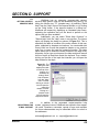
1. Getting context-sensitive help..........................................................65
2. Registering for e-mail support..........................................................65
3. Checking for updates ......................................................................67
E. APPENDICES
1. Taskbars .........................................................................................69
2. A typical analysis scenario ..............................................................70
3. Bibliography ....................................................................................74
6
User Guide
WinBreak
SECTION A. GENERAL
A.1
INTRODUCTION
WinBreak
The gas exchange or ventilatory threshold has had a long
history in exercise science and cardiorespiratory medicine. It is
also a concept that has sparked considerable controversy over
the years, particularly when interpreted as an index of the socalled anaerobic threshold or as causally related to the lactate
threshold (Meyers & Ashley, 1997; Svedahl & MacIntosh, 2003).
Yet, despite the controversy, the concept has persisted, as it
continues to be regarded by many as a useful practical marker of
cardiorespiratory fitness and endurance capacity, a more
appropriate, individually tailored criterion for exercise
prescriptions compared to various arbitrary percentages of
maximal capacity, and a meaningful non-invasive clinical
measure of cardiorespiratory health.
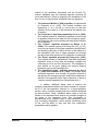
In fact, it could be argued that the gas exchange
threshold would have enjoyed a much greater popularity among
scientists and practitioners if it was not for certain difficulties
related to its determination. First, the difficulty lies in the fact that
the scientific literature contains a wide variety of possible indices
of the gas exchange threshold and the comparative evaluations
of the validity and reliability of these indices do not always agree.
The diversity of approaches is remarkable. The literature
includes proposals focused on VCO2 by VO2 plots, the ventilatory
equivalents, excess CO2 production, the respiratory exchange
ratio, ventilation and ventilatory frequency, and heart rate, among
several others (Anderson & Rhodes, 1989; Hughson, 1984;
Svedahl & MacIntosh, 2003). Second, most of the proposed
indices rely on subjective criteria for determining a "breakpoint,"
or change in the slope of plotted ventilatory data. Given the often
erratic nature of such data, this subjectivity commonly leads to
guesswork, a situation that makes trained scientists feel
uncomfortable.
As a solution to the problems associated with the
subjective nature of the traditional methods of determination,
there have been several attempts to develop computerized
methods, based on certain "objective" criteria. Specifically, such
attempts have focused on (a) piecewise (2- or 3-phase) linear
regression analyses, to identify a piecewise solution that
provides a better fit to the data compared to a singular linear
solution (e.g., Beaver et al., 1986), (b) time series analyses
(combined with other methods, such as hidden Markov chains),
to identify a breakpoint while accounting for serially correlated
noise in the data (e.g., Kelly et al., 2001), (c) fitting smoothing
spline functions and examining the form of the derivatives (e.g.,
Sherrill et al., 1990), and others. While these approaches
constitute significant advances, most have not found their way
into day-to-day practice because (a) some of the mathematical
concepts involved are complex and far-from-easy to implement
User Guide
7
independently and (b) the researchers who proposed these
methods have not made any software programs to perform the
necessary computations publicly available. Today, some
integrated metabolic analysis software packages offer a method
for the "automatic" estimation of the gas exchange threshold
(usually based on the "V-slope" method proposed by Beaver et
al., in 1986 or the "simplified V-slope" method proposed by Sue
et al. in 1988), but the exact methods used are poorly
documented and the computational details are not disclosed.
Furthermore, since all methods can and do fail to produce
satisfactory solutions in the cases of certain data sets, relying on
a single method of determination leaves users with no recourse
in cases of unsatisfactory solutions, other than having to resort to
subjective criteria.
WinBreak was developed to address these problems.
This is achieved by (a) combining the intuitive appeal of graphical
methods with the objectivity of statistical modeling, (b) offering
multiple parallel methods of determination as opposed to a single
method, and (c) allowing users to experiment with a variety of
solutions and visualization options. Specifically, following Gaskill
et al. (2001), WinBreak uses the following three graphical
methods:
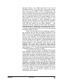
1. The V-slope method: This method consists of plotting CO2
production over O2 utilization and identifying a breakpoint in
the slope of the relationship between these two variables.
The level of exercise intensity corresponding to this
breakpoint is considered the gas exchange threshold.
2. The method of the ventilatory equivalents: This method
consists of plotting the ventilatory equivalents for O2 (VE/VO2)
and CO2 (VE/VCO2) over time or over O2 utilization and
identifying the level of exercise intensity corresponding to the
first rise in VE/VO2 that occurs without a concurrent rise in VE/
VCO2.
3. The Excess CO2 method: This method has been
operationalized in various ways. In WinBreak, the
operationalization of Excess CO2 follows that proposed by
Gaskill et al. (2001). According to their definition, Excess CO2
= (VCO22 / VO2) - VCO2. When Excess CO2 is plotted over
time or over O2 utilization, the gas exchange threshold is
thought to occur at the level of exercise intensity
corresponding to an increase in Excess CO2 from steady
state.
WinBreak produces the plots required for implementing
these three methods with one mouse click, enabling users to
obtain a quick graphical representation of the their data.
Furthermore, using a feature called the "Visualization Tool",
WinBreak applies mathematical algorithms designed to identify a
breakpoint in the plotted relationships. Specifically, for the
8
User Guide
WinBreak
method of the ventilatory equivalents and the Excess CO2
method, WinBreak uses the standard algorithm proposed by
Jones and Molitoris (1984) for identifying the breakpoint of two
lines. For the V-slope method, WinBreak uses five algorithms:
1. The Jones and Molitoris (1984) algorithm, as implemented
by Schneider et al. (1993). This method considers two
regressions, y = b0 + b1x and y = b0+b1x0+b3(x-x0), and then
searches for the value of x0 that minimizes the residual sum
of squares.
2. The "brute force" algorithm proposed by Orr et al. (1982).
This method consists of calculating regression lines through
all possible divisions of the data into two contiguous groups,
and finding the pair of lines yielding the least pooled residual
sum of squares.
3. The "V-slope" algorithm proposed by Beaver et al.
(1986). This method consists of dividing the VCO2 by VO2
curve into two regions, fitting linear regressions through them,
and identifying the point at which the ratio of the distance of
the intersection point from a single regression line through
the data to the mean square error of regression is maximized.
4. The "Dmax" algorithm proposed by Cheng et al. (1992).
This method consists of calculating a third-order polynomial
regression curve to fit the data and drawing a straight line
connecting the first and last data points. The breakpoint is
then defined as the point yielding the maximal distance
between the curve and the straight line.
5. The "simplified V-slope" algorithm proposed by Sue et
al. (1988) and Dickstein et al. (1990). This method again
calculates regression lines through all possible divisions of
the data into two contiguous groups, and finds a breakpoint at
which the first regression has a slope of less than or equal to
1 and the second regression has a slope higher than 1.
In addition, WinBreak allows users to examine the
complete computational details of all these methods, to compare
the fit of the two-regression solutions to a single-regression
solution, and to view and contrast plots of the residuals produced
by these solutions. Finally, WinBreak allows users to shift the
location of the breakpoint and observe the resultant changes in
the slope of the regression lines. This functionality is
supplemented by an extensive array of data manipulation tools
(e.g., averaging, interpolation, outlier removal, smoothing), ease
of use, and the ability to save and print fully customized,
presentation-quality graphics.
WinBreak
User Guide
9
A.2
SUMMARY OF FEATURES
•
•
•
•
•
•
•
•
•
•
•
•
•
•
A.3
SYSTEM REQUIREMENTS
10
Only such product in the world
Automated and integrated analysis and presentation of data
The most popular and powerful graphical methods for
identifying the gas exchange threshold, combined with nearly
all the statistical methods that have been proposed in the
exercise physiology literature
Complete computational details
Extensive array of data manipulation options (averaging,
interpolation, outlier removal)
Five methods of data smoothing (running-window average,
low-pass FFT filter, Savitzky-Golay least squares filter, cubic
spline filter, polynomial from second to tenth order)
Plots of residuals
Fully customizable graphics (labels, fonts, axis scaling,
symbol styles, line styles, sizes, and colors)
Graphical printouts accompanied by summary of
computational results
Ability to save graphics in Windows® Metafile and bitmap
formats, compatible with most major word processors and
presentation packages
Reads data in ASCII format and saves data in ASCII
(comma-delimited, tab-delimited) and Microsoft® Excel®
formats
Easy to use; very short learning curve
Great as an educational tool
Inexpensive
WinBreak was developed for IBM®-compatible computers
running the Microsoft® Windows® (Win32) operating system. This
includes all 32-bit variations of Windows®, including Windows
95®, Windows 98®, Windows 98 SE®, Windows NT®, Windows
XP®, Windows 2000®, etc.
Although the main executable file is approximately 4 MB,
the total free disk space required for installation is around 23 MB.
Any generated data and graph files will require additional disk
space.
In terms of hardware, a computer with an Intel® Pentium®
processor at 300 MHz and 64 MB of RAM will suffice, although
the data processing and graphing speeds will improve with more
advanced configurations.
User Guide
WinBreak
A.4
INSTALLATION
WinBreak may arrive in one of two forms: (a) on an
installation CD or (b) in a zip file downloaded from the internet. In
the latter case, you will have to first un-zip the file to retrieve its
contents. This can be accomplished by several utilities, such as
WinZip® (http://www.winzip.com) or PKzip® (http://www.pkzip.
com).
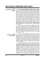
From the Windows® "Start" menu, select "Run…". Then,
click on "Browse…" and direct the file browser to the WinBreak
"Setup" program, located on the CD or in the directory in which
you expanded the contents of the zip file. This will execute the
WinBreak installation program. The first dialog box that will
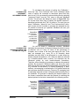
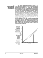
appear will be similar to the one shown in Figure A.1. The
default installation directory is called "WinBreak" and is located
within the "Program Files" directory on the C: drive. If you wish to
Figure A.1. If
you want to
install
WinBreak in a
different
directory, click
on "Change
Directory". To
install, click the
big square
button.
change this location and, instead, install WinBreak elsewhere,
click on the button labeled "Change Directory" and select the
desired location. To install WinBreak, click on the big square box
with the computer icon.
The installation program will copy the required files to the
selected location and register several additional system files (see
Figure A.2). During this process, the installation program may
detect that your computer already has newer versions of these
system files. In this case, choose to keep your existing files since
system files are supposed to be backwards compatible. In
addition to the core WinBreak executable, the installation
program will also copy a modifiable configuration file (winbreak.
cfg), some sample data files in a sub-directory named "Data" and
a copy of this user guide in Portable Document Format (PDF) in
a sub-directory named "manual." To uninstall WinBreak, select
"WinBreak" from the "Add/Remove Programs" Control Panel.
Figure A.2.
The installation
program will
copy and
register all the
required files
automatically.
WinBreak
User Guide
11
SECTION B. WORKING WITH DATA
B.1
ACCEPTABLE DATA FILE
FORMAT
To ensure compatibility with metabolic analysis systems
and software packages, WinBreak accepts data files in ASCII
format, since most software programs that accompany metabolic
analysis systems can export data in this format. Although the
structure of the data files varies widely from system to system
(and, in some cases, can even be customized), all ASCII data
files have certain similarities that allow WinBreak to read the
data. Specifically, all files include several lines at the top that
contain information about the participant and the conditions of
the test (these lines are ignored by WinBreak) and then list the
data either in comma-delimited, tab-delimited, or fixed-width
form. WinBreak reads the entire data matrix, but only uses the
following four variables: (a) time, (b) oxygen uptake, (c) carbon
dioxide production, and (d) ventilation. More details on how to
customize WinBreak to read data from your metabolic analysis
system are presented in the section entitled "Changing the data
file settings".
Note that, if a system does not export data in ASCII
format, but can export data in formats recognized by some other
spreadsheet or database program (e.g., Microsoft® Excel®), you
can use that other program to convert the data to ASCII. Finally,
also note that WinBreak will "remember" both the location of your
data files and the file extension of these files (e.g., PRN, CSV,
DAT, etc), to facilitate and accelerate the process of accessing
and reading your data.
B.2
CHANGING THE DATA
FILE SETTINGS
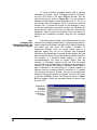
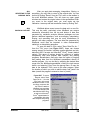
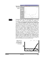
When you start WinBreak for the first time, you must
specify the structure of the data files produced by your metabolic
analysis system, so that WinBreak can read and meaningfully
interpret the data. To do this, select "Data File Settings" from the
"File" menu in the main WinBreak window. The dialog box shown
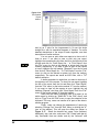
in Figure B.1 will appear. This procedure typically needs to be
carried out only once (unless you change your metabolic analysis
software). WinBreak will save your settings and reuse them the
next time you start it.
First, you must open one of the data files exported by
your metabolic analysis system, using an ASCII text editor (e.g.,
the Windows® Notepad® program), and count the number of lines
at the top of the file that contain information other than numerical
metabolic analysis data. Typically, the first lines will contain
information about the test subject, the date of the test, the
temperature, etc. Make sure that your count does not include
"wrapped" lines (in Notepad®, set the "Word Wrap" option off),
but does include lines that contain data column labels (e.g.,
"Time", "VE", "VO2", "RER", etc). In the dialog box, you can use
the drop-down menu marked "Lines to Ignore from the Top" to
specify how many lines at the top of the data file do not contain
12
User Guide
WinBreak
Figure B.1. The
dialog box used to
change the data file
settings
numerical metabolic data.
Second, you must specify the number and the name of
the data columns in your data files. On the left side of the dialog
box shown in Figure B.1, there is a list of variables commonly
found in metabolic analysis data files. You can either (a) select
labels from the list and click "Add" to add them to WinBreak's
"Data Column Labels" list (you can also double-click on the label)
or (b) you can type your own labels in the text box under "Type or
Select from the List" and click "Add" to add them to the list.
WinBreak will automatically count the labels as you add them. It
is very important that you enter exactly as many data labels as
there are data columns in your data files and that you specify the
correct order.
As you are entering the data column labels, WinBreak will
try to detect the position of the following four variables: (a) time [a
data label "Time"], (b) oxygen uptake [a data label "VO2" or "VO2
(L/min)"], (c) carbon dioxide production [a data label "VCO2" or
"VCO2 (L/min)"], and (d) ventilation [a data label "VE"]. If your
metabolic system uses milliliters instead of liters as the unit of
measurement, use "VO2" and "VCO2" as labels for the
respective columns. Since, by convention, WinBreak uses L/min,
it will automatically convert milliliter values to liters when reading
the data. WinBreak will show the position of the four variables
that it has detected
Note that, in case of duplicate entries in the "Data Column
Labels" list, WinBreak will warn you, but will accept the duplicate
entry if you confirm that this is what you want to do. Keep in
mind, however, that, if you make duplicate entries for the four
variables of primary interest (Time, VO2, VCO2, and VE),
WinBreak will consider as valid entries the ones listed last.
Check to ensure that the number and the order of data
column labels are correct. If necessary, you can change the
order by highlighting a label and clicking the up or down arrow
keys to change its position on the list. You may also highlight a
label and click "Remove" to delete it from the list. When finished,
click "OK" to close the dialog box and continue.
WinBreak
User Guide
13
B.3
LOADING NEW SETTINGS
The data file settings, as well as numerous other settings,
including all graph formatting settings, are automatically saved
when users exit the program in a file called "winbreak.cfg"
located in the WinBreak root directory. Therefore, users will
always restart the program with the same settings they were
using when they last exited the program. While this is convenient
in most cases, some additional flexibility is required for
laboratories with multiple metabolic analysis systems and
software packages. For these situations, WinBreak allows users
to save and subsequently load multiple alternate settings files.
This way, they can switch from data files generated with one
metabolic analysis software package to data files generated with
another software package with just one intermediate step,
instead of having to edit the data file settings (as described in
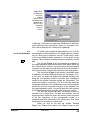
section B.2). To load a new settings file, select "Load New
Settings…" from the "File" menu in the main WinBreak window,
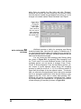
as shown in Figure B.2.
Figure B.2. To load
new settings from a
file, select "Load New
Settings" from the
"File" menu in the
main WinBreak
window.
The dialog box that will appear will allow you to search
your computer for files with the extension ".cfg", the default
extension for WinBreak settings files. Select the settings file that
you want to use and click on "Open". You have to make sure that
any data files you open after this point conform to the settings
specified in the newly loaded settings file. Otherwise, the data
will not be loaded properly or WinBreak may be unable to
operate.
You can also modify or edit the file settings at any time
and save the new settings for future use. The procedure for
saving settings files is explained in the next section.
14
User Guide
WinBreak
B.4
SAVING THE SETTINGS
Once you have made changes to the WinBreak settings,
regardless of whether they were changes to the data file settings
or to graph formatting, you can save the settings to a
configuration file for future use. This way, if you ever want to
reuse these settings, you would only need to load the particular
settings file instead of having to re-create all the changes
manually. To save the current settings, select "Save Settings
As…" from the "File" menu in the main WinBreak window, as
shown in Figure B.3. In the dialog box that will appear, you will
be asked to specify a file name for the new settings file. The
default file extension for WinBreak settings files is ".cfg".
Therefore, if you omit a file extension, the extension ".cfg" will be
added. If you specify a file name that already exists in the same
location, WinBreak will ask for a confirmation but, upon
confirmation, will overwrite the older file.
Also note that you can overwrite the default settings file
"winbreak.cfg" if you specify this as the file name for your
settings file. However, if you subsequently make additional
changes to the settings, these will be overwritten again when you
exit WinBreak. The reason is that WinBreak always overwrites
"winbreak.cfg" with the settings that are selected when the user
exits the program. This allows WinBreak to start by recalling the
same settings that were selected the last time that the program
was used. Therefore, overwriting "winbreak.cfg" is generally not
recommended and WinBreak will issue an alert when users try to
do so.
Figure B.3. To save
the current settings to
a file for future use,
select "Save Settings
As" from the "File"
menu in the main
WinBreak window.
WinBreak
User Guide
15
B.5
OPENING A DATA FILE
Before you open a data file, you must specify the
sampling or averaging rate that was used to produce the data in
the file. Use the up and down arrow keys in the frame marked
"Sampled/Averaged Every" to change your selection. Use "0" for
breath-by-breath sampling. If you need averaging, WinBreak can
do that for you (see the section titled "Data Averaging and
Filtering"). WinBreak will remember your selection and present it
as the default option the next time you use it.
To open a data file, click on "Open Data File" from the
"File" menu, as shown in Figure B.4. Alternatively, you can also
click on the file folder icon on the toolbar. In the dialog box that
will appear, you can change the default extension, to see a full
listing of the files in each folder. WinBreak will remember the
extension of the file you choose, as well as the location of the
file, so you will not have to look around to locate your data files
the next time you use the program.
Opening a data file will fill the spreadsheet with the data
in the file. The data are displayed to allow you to examine them
visually, but you cannot directly edit individual values through the
WinBreak spreadsheet. If you need to filter out aberrant values,
you can do that through WinBreak's outlier removal and data
averaging facilities.
If, upon reading the data file, WinBreak determines that
the data are expressed in milliliters, it will convert the VO2 and
VCO2 data to liters and will inform you of the conversion in the
frame marked "Unit Conversions".
Figure B.4. To open
a data file, you can
select the option from
the "File" menu or
click on the open file
folder icon on the
taskbar.
16
User Guide
WinBreak
B.6
DATA FILE PROPERTIES
To examine the properties of an open data file, click on
"Data File Properties" from the "File" menu in the main WinBreak
window. A window similar to the one shown in Figure B.5 will
appear. The properties shown include the name, extension,
location, and size of the file, the dates that the file was created,
modified, and accessed for the last time, as well as the settings
used in reading the file.
Figure B.5.
The window
showing the
properties of
a data file..
B.7
CLOSING A DATA FILE
To close the data file that is presently open, you can
select "Close" from the "File" menu or simply click the button
marked "X" on the toolbar, as shown in Figure B.6. This will
close any open graph windows and clear the spreadsheet.
Figure B.6. To
close a data file,
you can select
the option from
the "File" menu
or click on the
button marked
"X" on the
taskbar.
WinBreak
User Guide
17
B.8
SETTING THE
CALIBRATION/WARM-UP
AND TEST TERMINATION
TIMES
Before you can process and analyze your data, you must
specify the calibration or warm-up and test termination times.
This will instruct WinBreak to ignore any data points before and
after the actual testing protocol.
In order to quickly scroll around large data sets, users can
click on the four arrow buttons on the taskbar. These will scroll
the viewable part of the spreadsheet, so that one can see the top
or bottom row, and left-most or right-most data column with a
single mouse click. You can then click on the up and down arrow
keys in the frames marked "Calibration/Warm-Up" and "Test
Continued Until", to set the calibration or warm-up and test
termination times, respectively, as shown in Figure B.7.
WinBreak will remember your selections the next time you use it.
Presumably, the calibration/warm-up period will be constant for
each testing protocol. The test termination time may be the same
for experimental conditions with fixed duration or may vary from
one test participant to the next in the case of tests of maximal
capacity or time-to-exhaustion protocols.
After making your selections, click the button marked
"Set" to finalize your settings. This will display (a) the index of the
first row of data to be included in the analyses, (b) the index of
the last row of data to be included in the analyses, (c) the total
number of data rows to be considered in the analyses, and (d)
the highest recorded value of oxygen uptake in a status bar
panel at the bottom of the main WinBreak window.
Figure B.7. After you open
a data file, use the up and
down arrow keys to set the
calibration / warm-up and
test termination times.
Then, press "Set" to fix
these times.
18
User Guide
WinBreak
B.9
CHANGING THE
INCREMENT /
DECREMENT PERIOD
To accelerate the process of setting the "Calibration /
Warm-Up" and "Test Continued Until" times, WinBreak allows
users to specify the increment or decrement period that they
want to use. You can access the relevant dialog box by selecting
"Increment Period" from the "File" menu in the main WinBreak
window. This will open the dialog box shown in Figure B.8. Use
the up and down arrow keys to specify the desired increment /
decrement period and click "OK" to continue. The next time you
select "Calibration / Warm-Up" and "Test Continued Until" times,
each mouse click will increase or decrease the selected time by
the number of seconds you specified. WinBreak will save your
preference and reuse it.
Figure B.8.
The increment /
decrement
period is used
to adjust the
warm-up and
test termination
times.
B.10
CHANGING THE
AVERAGING PERIOD FOR
ESTIMATING VO2peak
As will be shown in subsequent sections, WinBreak
estimates the occurrence of the gas exchange threshold in terms
of absolute VO2 (in L/min), in terms of the percentage of
VO2peak, and in terms of the time point during the test. If the
data are averaged (e.g., every 20 or 30 seconds), these
estimates are less likely to be influenced to a great extent by
breath-to-breath fluctuations in VO2. When the data are collected
on a breath-by-breath basis, however, the estimates can be
influenced greatly by such breath-to-breath fluctuations.
Therefore, some averaging is necessary to address this potential
problem. By convention, WinBreak retains and shows the exact
time point at which the gas exchange threshold occurred and the
VO2 recorded at that breath (i.e., without averaging). It does,
however, use averaging in estimating the %VO2peak at which the
gas exchange threshold occurred. It does so by averaging both
in estimating VO2peak and the %VO2peak attained at the point of
the threshold. The process for selecting the desired options for
the former is described here and the process for selecting the
desired options for the latter is described in the following section.
Figure B.9.
Select the
averaging
period used in
estimating
VO2peak.
WinBreak
User Guide
19
To set the desired averaging period used in deriving
estimates of VO2peak, select "Averaging Period for VO2peak"
from the "File" menu in the main WinBreak window. This will
open the dialog box shown in Figure B.9. You can choose to
estimate VO2peak based on data averaged every 15, 20, 30, or
60 seconds. Use the drop-down menu to make your selection
and click "OK". If no data set is open or if the calibration / warmup and test termination times have not been set, WinBreak will
simply store this value for future use. If a data set is open and the
calibration / warm-up and test termination times have been set,
WinBreak will re-calculate VO2peak using the new averaging
period.
B.11
CHANGING THE
AVERAGING PERIOD FOR
ESTIMATING %VO2peak
Particularly when the data in the WinBreak data set were
collected on a breath-by-breath basis, it is possible that values of
oxygen uptake will fluctuate, with high values being followed by
low values and vice versa. This creates a problem for
subsequent analyses, since the oxygen uptake value at a
particular breath may not be an accurate and informative
reflection of the percentage of maximal aerobic capacity that had
been reached at the time (or workload) that the breath occurred.
For example, if a particular breath happens to yield an
uncharacteristically low value of oxygen uptake, then the
estimate of %VO2peak reached at the time that the breath
occurred will be an underestimate. Therefore, some averaging is
necessary to address this problem. WinBreak allows users to
derive estimates of the percentage of VO2peak reached at
different times by averaging either 5-9 seconds or 3-7 breaths
surrounding the breath in question. You can set this period by
selecting "Averaging Period for %VO2peak" from the "File" menu
in the main WinBreak window. The dialog box shown in Figure
B.10 will appear. Select the averaging period you want to use
and click "OK".
Figure B.10.
Select the
averaging
period used in
estimating %
VO2peak.
20
User Guide
WinBreak
B.12
DESCRIPTIVE STATISTICS
To get a quick view of the statistical characteristics of a
data set, you can select "Descriptive Statistics" from the "Tools"
menu of the main WinBreak window. This will open the dialog
box shown in Figure B.11.
WinBreak calculates the mean, standard deviation,
variance, skewness, kurtosis, minimum, and maximum values of
VO2, VCO2, and VE. Skewness and kurtosis are calculated by the
formulas shown below:
n
xi − x
Skewness =
∑
(n − 1)(n − 2) S
3
4
3(n −1)2
n(n + 1)
xi − x
Kurtosis =
−
∑
(n −1)(n − 2)(n − 3) S (n − 2)(n − 3)
Figure B.11. In the
Descriptive Statistics
dialog box,
WinBreak displays
the mean, standard
deviation, variance,
skewness, kurtosis,
minimum, and
maximum of VE,
VO2, and VCO2.
B.13
REMOVING OUTLIERS
WinBreak
Occasionally, due to a malfunction in the data collection
equipment or the interface between the metabolic analysis
hardware and software, certain aberrant values, clearly outside
the physiological range, may be recorded in your data set. Such
values would obviously lead to erroneous results if they were to
be included in the statistical analysis of gas exchange data.
Therefore, WinBreak offers a facility that allows users to remove
rows of data containing values of VO2, VCO2, or VE that exceed
certain limits. This facility is accessible, after you set the
"Calibration / Warm-Up" and "Test Continued Until" times, by
selecting "Remove Outliers" from the "Tools" menu in the main
WinBreak window. The dialog box shown in Figure B.12 will
appear.
WinBreak will automatically display the mean, standard
deviation, minimum, and maximum value for VO2, VCO2, or VE in
the frame entitled "Descriptive Statistics". It will also fill in the
boxes marked "Lower Than" and "Higher Than" with the values
corresponding to the mean ± 4 standard deviations (or 0.1 if
subtracting 4 standard deviations from the mean results in a
negative number) for VO2, VCO2, and VE. You can change these
numbers to set the upper and lower limits of the filter as you
User Guide
21
wish. Once you specify the filter limits and click "Process,"
WinBreak will remove the rows containing out-of-bounds values
from the data set, update the spreadsheet, and inform you of the
changes in the areas marked "Rows Eliminated" and "Report".
Figure B.12.
Change the
"Lower Than"
and "Higher
Than" values to
filter out rows of
data containing
data values that
fall outside these
limits.
B.14
DATA AVERAGING AND
FILTERING
22
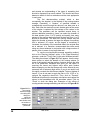
WinBreak provides a facility for averaging and filtering
breath-by-breath data. Note that this option is available only if
you have specified that the data in the data file were sampled on
a breath-by-breath basis. Otherwise, WinBreak assumes that the
data have already been averaged.
You can access the data averaging and filtering dialog
box, shown in Figure B.13, by selecting "Data Averaging" from
the "Tools" menu in the main WinBreak window. From the data
averaging options, you can choose to average 15-sec, 20-sec,
30-sec, or 60-sec segments. From the data filtering options, you
can choose to ignore aberrant values during the averaging
process, by setting a cut-off at 3, 5, 10, 20, or 50 times smaller or
larger than the average of the two adjacent values. This should
help you eliminate non-physiological values that were recorded
due to an equipment malfunction. Note that this filtering is only
applied to the VO2, VCO2, and VE values. After pressing "OK",
WinBreak will perform the necessary calculations and present
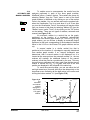
the averaged data in the spreadsheet. An example of the effects
of data averaging (20-seconds) is shown in Figure B.14.
User Guide
WinBreak
Figure B.13.
In the case of
breath-bybreath data,
you can
choose an
averaging
period and
direct
WinBreak to
ignore data
points that
exceed
certain limits.
Figure B.14.
An example
of VE/VO2
data
averaged
every 20
seconds.
40
Raw
38
Averaged (20 sec)
36
34
32
30
28
26
24
22
20
0
5
10
15
20
25
Time (min)
B.15
DATA INTERPOLATION
WinBreak
Occasionally, you may wish to transform data that were
collected on a breath-by-breath basis and, therefore, at irregular
time intervals to data that are equally spaced in time. The
procedure used to accomplish this is called interpolation.
Specifically, WinBreak uses polynomial interpolation. This means
that each interpolated value is calculated by fitting a polynomial
curve to the 3 or 5 data points surrounding a certain time point
and then estimating what the value of VO2, VCO2, and VE would
be at that time point on the basis of the polynomial.
To access the data interpolation facility offered by
WinBreak, select "Data Interpolation" from the "Tools" menu of
the main WinBreak window. The dialog box shown in Figure
B.15 will appear. First, select whether you wish to use polynomial
curves fitted over the 3 or 5 data points surrounding each time
point (1 before and 2 after or 2 before and 3 after, respectively).
The 5-point interpolation is generally recommended because it is
less susceptible to single extreme values and wild fluctuations in
the data that could produce even more extreme interpolated
values due to the relative inflexibility of polynomials.
User Guide
23
Figure B.15. To transform
breath-by-breath data to
data that are equally
spaced in time, use data
interpolation. Select
whether you wish to use
polynomial curves fitted
over 3 or 5 points and
what the time interval of
your data should be.
Figure B.16. An
example of VE/
VO2 data
interpolated at 5second (top) and
10-second
(bottom)
intervals.
40
Raw
38
Interpolated (5 sec)
36
34
32
30
28
26
24
22
20
0
5
10
15
20
25
Time (min)
40
Raw
38
Interpolated (10 sec)
36
34
32
30
28
26
24
22
20
0
5
10
15
20
25
Time (min)
24
User Guide
WinBreak
Then select the desired time interval of the new,
interpolated data set. Notice that you can choose to obtain data
spaced every 5 to 12 seconds. If you wish to obtain regularly
spaced data at longer time intervals, then use data averaging, an
option that allows you to obtain data spaced every 15 to 60
seconds.
After you make your selections, click "OK". WinBreak will
perform the necessary calculations and update the spreadsheet
with the interpolated values. Examples of data interpolated every
5 and 10 seconds (with 5-point polynomials) are shown in Figure
B.16.
Occasionally, if one or more of the first data points in the
original breath-by-breath data set occur after the first time
interval (e.g., if you have chosen a 5-second time interval and the
first recorded breath occurred at the 6th second), the data
interpolation procedure will produce zero values for those early
time points. In such cases, WinBreak will remove these rows of
data and inform you of this occurrence. Also note that,
occasionally, breath-by-breath data sets may contain duplicate
entries for time (e.g., two, typically consecutive, data points
recorded as having occurred at the same millisecond). Because
the data interpolation algorithm cannot function with duplicate
entries in the abscissa, WinBreak will replace any rows
containing duplicate time values with a single row containing the
average values of the replaced rows and inform you that this
operation has taken place.
B.16
SMOOTHING BY MOVING
WINDOW AVERAGE
WinBreak
Changes in the ventilatory indices used by WinBreak to
detect the gas exchange threshold are generally slow,
considerably slower than breath-to-breath and other ventilatory
fluctuations that are not of metabolic origin. This means that, for
the purposes of detecting the occurrence of the gas exchange
threshold, a certain degree of data smoothing (i.e., removal of
high-frequency components unlikely to be of metabolic origin)
may be helpful, both by facilitating the visual inspection of the
data and by reducing the possibility of adversely influencing the
breakpoint-detection algorithms. That said, data filtering must
generally be conservative and its results examined carefully. As
a case in point, although data smoothing, if done correctly, may
not shift the location of the gas exchange threshold within a data
set, it may nevertheless change the numerical estimate of the
level of O2 uptake at which the threshold occurred. It is,
therefore, recommended that data smoothing be used only when
necessary (i.e., in cases of highly convoluted data sets) and that
efforts be made to confirm any threshold-detection results
derived from smoothed data by also examining the raw data.
WinBreak uses five data smoothing methods, each based
on a different approach to smoothing. It is, therefore, important
that users familiarize themselves with the nature of each method
User Guide
25
and develop an understanding of the types of smoothing that
should be expected from each method. This should help them
determine which of the five methods would be most appropriate
in each case.
The first data-smoothing method, which is also
conceptually the simplest, is the method of the running-window
average. Essentially, a "window" of specified breadth is
systematically moved through the data set, one data point at a
time. Each time the window is moved, the data point at the center
of the window is replaced by the average of the values in the
window. The procedure can be repeated several times, to
achieve additional smoothing. Users can select the breadth of
the data window (from 5 to 25 points) and specify how many
passes of the running window through the data set (from 1 to 5)
should be performed. The wider the running window and the
higher the number of passes, the larger the degree of smoothing
that is achieved. Of course, as the degree of smoothing is
increased, the similarity of the smoothed data to the original data
set is reduced. It is, therefore, recommended that users avoid
using very broad windows in conjunction with a large number of
passes, even in cases of very large data sets.
To use the running-window average smoothing method,
click on the "Running Average" option, in the "Data Smoothing"
submenu, under the "Tools" menu in the main WinBreak window.
The dialog box shown in Figure B.17 will appear. Use the dropdown menus to select the breadth of the running window (in
terms of data points) and the number of passes through the data
set to be performed. WinBreak also gives you the option of
removing the lowest and highest value within each window
before averaging, so that the average will not be affected by any
extremely low or extremely high values. If you do not wish to use
this option, uncheck the check boxes labeled "Take out highest &
lowest". If you do not want to apply the filter to VO2, VCO2 or VE,
uncheck the respective check box. Then, click on "Process".
WinBreak will perform the necessary calculations and replace the
values in the spreadsheet with the smoothed values. Click on
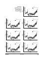
"Close" to close the dialog box. Examples of the effects of
running-window average smoothing can be found in Figure B.18.
Figure B.17. In
the runningwindow average
smoothing filter
dialog box,
select the
breadth of the
data window and
the number of
passes to be
performed.
26
User Guide
WinBreak
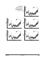
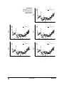
Figure B.18.
Examples of VE/VO2
data smoothed using
different options of
the running-window
average smoothing
filter.
40
Raw
38
Smoothed (15-pts, 1 pass)
36
34
32
30
28
26
24
22
20
0
5
10
15
20
25
Time (min)
40
40
Raw
38
Smoothed (15-pts, 2 passes)
36
36
34
34
32
32
30
30
28
28
26
26
24
24
22
22
20
0
5
10
15
20
25
Raw
38
20
Smoothed (15-pts, 3 passes)
0
5
10
Time (min)
40
40
Raw
38
Smoothed (15-pts, 4 passes)
36
34
34
32
32
30
30
28
28
26
26
24
24
22
22
0
5
10
15
20
25
20
0
5
10
40
Raw
38
Smoothed (20-pts, 3 passes)
36
34
34
32
32
30
30
28
28
26
26
24
24
22
22
10
25
15
20
25
20
Smoothed (25-pts, 3 passes)
0
Time (min)
WinBreak
20
Raw
38
36
5
15
Time (min)
40
0
25
Smoothed (15-pts, 5 passes)
Time (min)
20
20
Raw
38
36
20
15
Time (min)
5
10
15
20
25
Time (min)
User Guide
27
B.17
SMOOTHING BY LOWPASS FFT FILTER
The second data-smoothing method uses a Fast Fourier
Transform (FFT) low-pass filter. The Fourier transform
decomposes or separates a waveform or function into sinusoids
of different frequency which sum to the original waveform.
Through the use of a low-pass FFT filter, users can, therefore,
remove the high-frequency components of a physiological
waveform and leave only a small percentage of low-frequency
components. The assumption is that the breath-to-breath
variations, which will make up most of the high-frequency
components are not of metabolic origin. On the other hand,
changes in the relationships between VCO2 and VO2 or between
the ventilatory equivalent of oxygen and time, for example, which
may be significant from a metabolic standpoint change at a rate
that is much slower than breath-to-breath variations (Beaver et
al., 1986). Therefore, the prudent removal of the high-frequency
components should remove most of the ventilatory "noise" while
unveiling the slow changes that are of metabolic interest. For
more on the technical aspects of FFT, users are referred to
Brigham (1988; The Fast Fourier Transform and its applications,
Englewood Cliffs, NJ: Prentice-Hall) and Cooley and Tukey
(1965; An algorithm for the machine calculation of complex
Fourier series, Mathematics of Computation, 19, 297-301).
To use the low-pass FFT smoothing filter, click on the
"Low-pass FFT Filter" option, in the "Data Smoothing" submenu,
under the "Tools" menu in the main WinBreak window. The
dialog box shown in Figure B.19 will appear. Move the slider to
the left or right to set the desired cut-off percentage of the
frequency spectrum. The percentage shown indicates how much
of the frequency spectrum will be retained after the highfrequency components are filtered out. If you do not want to
apply the filter to VO2, VCO2 or VE, uncheck the respective check
box. Click on "Process". WinBreak will perform the necessary
calculations and replace the values in the spreadsheet with the
smoothed values. Click on "Close" to close the dialog box.
Examples of the effects of the low-pass FFT filter with different
cut-off frequencies can be found in Figure B.20.
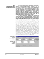
Figure B.19. In
the low-pass
FFT smoothing
filter dialog box,
select the
percentage of
the frequency
spectrum to be
retained.
28
User Guide
WinBreak
Figure B.20.
Examples of VE/VO2
data smoothed using
different frequency cutoff levels in the lowpass FFT filter.
40
Raw
38
Smoothed (Cut-off: 10%)
36
34
32
30
28
26
24
22
20
0
5
10
15
20
25
Time (min)
40
40
Raw
38
Smoothed (Cut-off: 8%)
36
36
34
34
32
32
30
30
28
28
26
26
24
24
22
22
20
0
5
10
15
20
25
Raw
38
20
Smoothed (Cut-off: 6%)
0
5
10
Time (min)
40
40
Raw
38
Smoothed (Cut-off: 4%)
36
34
34
32
32
30
30
28
28
26
26
24
24
22
22
0
5
10
25
15
20
25
20
Smoothed (Cut-off: 2%)
0
Time (min)
WinBreak
20
Raw
38
36
20
15
Time (min)
5
10
15
20
25
Time (min)
User Guide
29
B.18
SMOOTHING BY
SAVITZKY-GOLAY FILTER
The third data-smoothing method is the Savitzky-Golay
filter, described by Abraham Savitzky and Marcel J.E. Golay
(1964; Smoothing and differentiation of data by simplified least
squares procedures, Analytic Chemistry, 36, 1627-1639). The
procedure is similar to the running-window average method in
that a window of a certain width is systematically moved through
the data set, replacing each raw value with a combination of itself
and some nearby values. The difference is that, in the SavitzkyGolay procedure, the underlying function within the moving
window is approximated not by a constant whose estimate is the
average but by a higher-order polynomial.
To use the Savitzky-Golay smoothing filter, click on the
"Savitzky-Golay Filter" option, in the "Data Smoothing" submenu,
under the "Tools" menu in the main WinBreak window. The
dialog box shown in Figure B.21 will appear. Use the drop-down
menus to select the breadth of the running window (odd
numbers, from 5 to 25 data points) and the number of passes
through the data set to be performed (from 1 to 200). If you do
not want to apply the filter to VO2, VCO2 or VE, uncheck the
respective check box. Then, click on "Process". WinBreak will
perform the necessary calculations and replace the values in the
spreadsheet with the smoothed values. Click on "Close" to close
the dialog box. As is the case with the running-window average
smoothing filter, the wider the running window and the higher the
number of passes, the larger the degree of smoothing that is
attained. Examples of the effects of the Savitzky-Golay
smoothing procedure, used in conjunction with various
combinations of options, are shown in Figure B.22.
Figure B.21. In
the SavitzkyGolay smoothing
filter dialog box,
select the
breadth of the
data window and
the number of
passes to be
performed.
30
User Guide
WinBreak
Figure B.22.
Examples of VE/VO2
data smoothed using
different options of
the Savitzky-Golay
smoothing filter.
40
Raw
38
Smoothed (15 pts, 10 passes)
36
34
32
30
28
26
24
22
20
0
5
10
15
20
25
Time (min)
40
40
Raw
38
Smoothed (15 pts, 30 passes)
36
36
34
34
32
32
30
30
28
28
26
26
24
24
22
22
20
0
5
10
15
20
25
Raw
38
20
Smoothed (15 pts, 50 passes)
0
5
10
Time (min)
40
40
Raw
38
Smoothed (21 pts, 30 passes)
36
34
34
32
32
30
30
28
28
26
26
24
24
22
22
0
5
10
15
20
25
20
0
5
10
40
Raw
38
Smoothed (21 pts, 70 passes)
36
34
34
32
32
30
30
28
28
26
26
24
24
22
22
10
25
15
20
25
20
Smoothed (25 pts, 90 passes)
0
Time (min)
WinBreak
20
Raw
38
36
5
15
Time (min)
40
0
25
Smoothed (21 pts, 50 passes)
Time (min)
20
20
Raw
38
36
20
15
Time (min)
5
10
15
20
25
Time (min)
User Guide
31
B.19
SMOOTHING BY CUBIC
SPLINE CURVE FITTING
The fourth data-smoothing option is the cubic spline,
based on the computational procedures proposed by Carl de
Boor (1978; A practical guide to splines Applied Mathematical
Sciences Series, vol 27. New York: Springer-Verlag. pp. 240242) and implemented in the PPPACK algorithm. Spline
smoothing is based on the assumption that a smooth function
underlies the data and attempts to recover the function by
minimizing a smoothing parameter representing a compromise
between the desire to stay as close to the original data as
possible and the desire to obtain a smooth function.
To use the cubic spline smoothing filter, click on the
"Cubic Spline" option, in the "Data Smoothing" submenu, under
the "Tools" menu in the main WinBreak window. The dialog box
shown in Figure B.23 will appear. Users must select a value of
the parameter S, described by de Boor as the "upper bound on
the discrete weighted mean square distance of the approximation
from the data". In practice, there is rarely any basis for knowing
how to select this value for a given data set in advance. Thus, de
Boor notes that "more naively, S represents a knob which one
may set or turn to achieve a satisfactory approximation to the
data" (pp. 242-243). In other words, users may have to
experiment by selecting different values of S. Thankfully, in most
cases, the different values of S will have little effect on the shape
of the smoothing spline. If you do not want to apply the filter to
VO2, VCO2 or VE, uncheck the respective check box. Once the S
parameter has been set, click on "Process". WinBreak will
calculate the values of the smooth function and update the
spreadsheet. It will also present the values of the first derivative
of the spline function. Click on "Close" to close the dialog box. An
example of the effects of smoothing a data set using the cubic
spline smoothing procedure is shown in Figure B.24.
Figure B.23. In
the cubic
smoothing spline
dialog box,
select the value
of the S
parameter and
click on
"Process".
32
User Guide
WinBreak
Figure B.24. Example
of VE/VO2 data
smoothed using a
cubic smoothing
spline.
40
Raw
38
Smoothed (S = 10)
36
34
32
30
28
26
24
22
20
0
5
10
15
20
25
Time (min)
B.20
SMOOTHING BY
POLYNOMIAL
REGRESSION CURVE
FITTING
The fifth data-smoothing option is least-squares
polynomial regression. Polynomial regression equations are of
the form fx = a0 + a1x + a2x2 + … + anxn. WinBreak allows users to
fit polynomial curves of orders from second to tenth. Lower-order
polynomials are smoother, whereas higher-order polynomials
generally provide a closer fit to the original data.
To use the polynomial regression smoothing option, click
on the "Polynomial Regression" option, in the "Data Smoothing"
submenu, under the "Tools" menu in the main WinBreak window.
The dialog box shown in Figure B.25 will appear. First, use the
drop-down menus to select the degree of polynomial fit you wish
to obtain. If you do not want to apply the smoothing to VO2, VCO2
or VE, uncheck the respective check box. Then, click on
"Process". WinBreak will perform the necessary calculations and
replace the values in the spreadsheet with the smoothed values.
It will also display the a0 to an coefficients of the polynomial
regression equation. Click on "Close" to close the dialog box.
Examples of applying smoothing using polynomial regressions of
various orders are shown in Figure B.26.
Figure B.25. In
the polynomial
least-squares
regression
dialog box,
select the order
of the
polynomial and
click on
"Process".
WinBreak
User Guide
33
Figure B.26.
Examples of VE/VO2
data smoothed using
polynomials of
different orders.
40
Raw
38
Smoothed (Degree: 2)
36
34
32
30
28
26
24
22
20
0
5
10
15
20
25
Time (min)
40
40
Raw
38
36
36
34
34
32
32
30
30
28
28
26
26
24
24
22
22
20
0
5
10
15
20
Raw
38
Smoothed (Degree: 4)
25
20
Smoothed (Degree: 6)
0
5
10
Time (min)
40
40
Raw
38
36
34
34
32
32
30
30
28
28
26
26
24
24
22
22
0
5
10
15
20
25
20
Time (min)
34
20
25
Raw
38
Smoothed (Degree: 8)
36
20
15
Time (min)
Smoothed (Degree: 10)
0
5
10
15
20
25
Time (min)
User Guide
WinBreak
B.21
REVERTING TO THE
ORIGINAL DATA
After you apply data averaging, interpolation, filtering, or
smoothing, you may wish to return to the original data. You can
do this by clicking "Revert" from the "File" menu or the taskbar in
the main WinBreak window. This will close any open graph
windows and restore the original values in the spreadsheet. After
you revert to the original data, you must again set the
calibration / warm-up and test termination times by clicking "Set".
B.22
SAVING A DATA SET
WinBreak allows users to save the data set in a new file.
This may be useful, particularly since WinBreak can remove
extraneous information from the top and bottom of data files
generated by metabolic analysis software packages and can
perform additional operations, such as averaging, interpolating,
filtering, and smoothing that may be more cumbersome to
perform with other programs. The new data files generated by
WinBreak could then be imported in other mathematical,
statistical, or data-plotting programs.
To save the data in a file, select "Save Data File As…"
from the "File" menu (see Figure B.27). Users can choose
among several file formats, including comma-delimited and tabdelimited ASCII formats and Microsoft® Excel® format (default
option). This range of options should be sufficient to enable
compatibility with most popular data analysis and plotting
programs. Nevertheless, users also have the option of copying
and pasting data from the WinBreak spreadsheet directly to
another program. You can do this by selecting the desired data
range from the WinBreak spreadsheet, clicking the right mouse
button, and selecting "Copy" from the pop-up menu, to copy the
data to the clipboard. Then, move to the other program, select
the location at which you wish to add the data, and "paste" the
data (consult the program's manual on how to "paste").
Figure B.27. To save a
data set, select "Save
Data File As…" from the
"File" menu in the main
WinBreak window or click
the floppy computer disk
icon from the taskbar.
WinBreak can save data
in comma-delimited and
tab-delimited ASCII files,
as well as in Microsoft®
Excel® spreadsheets for
compatibility with other
data analysis and plotting
programs.
WinBreak
User Guide
35
SECTION C. WORKING WITH GRAPHS
C.1
THE GRAPH BROWSER
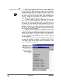
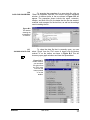
WinBreak offers a feature called "Graph Browser," which
allows users to obtain quick visual representations of the data
set. Specifically, the Graph Browser can display the 17 graphs
shown in the menu in Figure C.1. The different graphs are
available either from the drop-down menu or from the left and
right arrows on the task bar of the Graph Browser window, which
will rotate through the set of graphs in the same order shown in
the menu. Users can (a) save or print each graph by selecting
the respective options in the "File" menu or (b) rescale the axes
or customize each graph by selecting the respective options in
the "Graph" menu (see Figure C.2).
Figure C.1. The Graph Browser
can display the 17 different plots
shown in the menu. Use the
drop-down menu labeled
"Graph" to jump directly to a
certain graph or use the left and
right arrows on the task bar to
rotate through the set in the
same order shown here.
Figure C.2. In the Graph
Browser window, click on
the left and right arrows on
the taskbar to rotate
through the 17 different
plots of the data. Using the
other buttons on the
taskbar, you can save,
print, rescale, or customize
the graphs.
36
User Guide
WinBreak
C.2
THE RESPIRATORY
COMPENSATION POINT
During the initial stages of an incremental exercise test,
VE increases in proportion to CO2 output. This is called isocapnic
buffering. Thus, the relationship between VE and VCO2 is positive
linear. However, after the gas exchange threshold has been
exceeded and metabolic acidosis has occurred, VE starts to
increase more rapidly than VCO2. This accentuated ventilatory
response is called "respiratory compensation" (or "ventilatory
compensation"). Because the point where the respiratory
compensation starts must follow the gas exchange threshold, the
identification of this point is useful in the process of determining
the gas exchange threshold, as it can serve as the "upper
boundary" for the calculations involved in this process.
WinBreak includes a module for the detection of the point
of respiratory compensation. The module is accessible by
selecting "Find Respiratory Compensation Point" from the "Tools"
menu of the three graphical modules used for the determination
of the gas exchange threshold (i.e., the V-slope, ventilatory
equivalents, and Excess CO2 modules). Alternatively, users can
access this module by clicking on the button marked "RC" on the
taskbar. This will open the window shown in Figure C.3.
Figure C.3. The
module for the
determination of
the respiratory
compensation
point. Select the
desired
percentage of
difference
between the first
and second slope
in the relationship
between VE and
VCO2 and click
on "Find RC
Point".
The method implemented in WinBreak for the
determination of the respiratory compensation point generally
follows the recommendations by Beaver et al. (1986). According
to these authors, the respiratory compensation point is
determined as follows: "The VE vs. VCO2 data are divided into
two linear segments [i.e., two regions, each of which is fitted with
a linear regression]. The intersection of the two segments is the
[respiratory compensation] point if the change in slope between
them is greater than a preselected amount (15% of the initial
slope). If a [respiratory compensation] point is found, its location
WinBreak
User Guide
37
is transferred to the VCO2 vs. VO2 curve [see the V-slope
sections below] and used as the upper boundary for the
calculation [of the gas exchange threshold]. Certain subjects,
notably patients with obstructive lung disease, may not have a
[respiratory compensation] point" (p. 2023).
Figure C.4. The module for
the determination of the
respiratory compensation
point. Select the desired
percentage of difference
between the first and
second slope in the
relationship between VE and
VCO2 and click on "Find RC
Point".
To use the respiratory compensation module, use the
drop-down menus to select (a) the starting point for the
calculations and (b) the percentage by which you want the
second slope to be higher than the first, as shown in Figure C.4.
Option (a) is useful because, in some cases, the early data
points may include non-linear segments, which should be
excluded for the search of the actual respiratory compensation
point to be meaningful, as this usually occurs after the midpoint
of incremental exercise tests. Option (b) determines the amount
by which the slope of the second linear regression through the VE
by VCO2 data should be higher than the first. According to
Beaver et al. (1986), a reasonable number is 15%. In WinBreak,
you can select any number between 5% and 100%.
Once the two selections have been made, click on "Find
RC Point". WinBreak will compute all possible two-segment
regressions and then search (from beginning to end) for the first
occurrence of a slope difference that equals or exceeds the
percentage selected in the "Diff in Slopes" menu. It will then
present (a) the slope of the first regression, (b) the slope of the
second regression, (c) the percentage of difference between the
two slopes (which should be equal to or slightly higher than the
percentage selected in the "Diff in Slopes" menu), (d) the
maximum slope difference found in the data set, and (e) the
location (in terms of VO2 and time) of the maximum slope
difference. WinBreak will also re-plot the VE by VCO2 graph,
38
User Guide
WinBreak
showing the two regression lines through the data. The symbols
representing the data points of the first and second regressions
(as well as any data points excluded from the early phases of the
data set) can also be different, to facilitate the visual inspection of
the results.
Depending on how small the selected percentage of
difference is between the slopes of the second and first
regressions, it is possible that, upon visual inspection, users may
decide that the automatically determined point is a nonsatisfactory estimate of the respiratory compensation point. In
such cases, users can manually shift the location of the tentative
respiratory compensation point higher or lower either by clicking
on the left and right arrows (for small shifts) or by using the dropdown menu (for larger shifts) and clicking on the button marked
">>", as shown in Figure C.5.
Figure C.5. Click on the left and
right arrows or use the dropdown menu to manually shift
the tentative respiratory
compensation point.
WinBreak will respond by re-plotting the regression lines
and re-calculating the regression slopes, as well as the
percentage of difference between them. Alternatively, users may
opt to change the desired percentage of difference between the
second and first slopes and perform a new search for a tentative
respiratory compensation point. Any change in the "Diff in
Slopes" menu will reset the panel, delete any previous results,
and return the VE by VCO2 graph to its original state, with no
visible regression lines.
For users who wish to receive additional information
about the calculations that were involved in selecting a tentative
respiratory compensation point, WinBreak offers a complete
account. This is available by clicking the tab entitled "Detailed
Report". Each time a search for a tentative respiratory
compensation point is performed, the Detailed Report will include
the results of all the regression analyses involved.
Finally, once a satisfactory respiratory compensation
point has been identified, users can click on "Transfer", as shown
in Figure C.6, to make that data point the upper boundary in the
calculations for determining the gas exchange threshold.
Figure C.6. Once a satisfactory
respiratory compensation point
has been identified, click on
"Transfer" to set this data point
as the upper boundary for the
gas exchange threshold
calculations.
WinBreak
User Guide
39
C.3
THE V-SLOPE METHOD
IN GENERAL
The first method for detecting the gas exchange threshold
offered by WinBreak is the V-slope, originally described by
Beaver et al. (1986). The method consists of plotting CO2
production against O2 utilization and identifying a breakpoint in
the relationship between these two variables. This is achieved
mainly by computing linear regressions based on two contiguous
segments of the data, and identifying a point that yields a
substantial increase in the slope of the second regression
compared to the first.
Although the visual identification of a breakpoint in the
VCO2 by VO2 relationship may be relatively easy in many cases
of averaged data, it often proves very difficult in the case of
breath-by-breath data due to the densely cluttered data points,
the frequent fluctuations of VO2 and VCO2 from higher to lower
values, and various kinds of breath-to-breath irregularities.
Similar difficulties also impact the statistical methods used for the
determination of a breakpoint, since it is possible that even a
single erratic data point (with large "leverage") can cause a
transient but large change in the slope of a regression.
Therefore, some type of averaging or interpolation of data is
generally recommended, particularly in the case of large data
sets, before using the V-slope method.
To display the V-slope graph window, click on "Show
VCO2 by VO2 Graph" from the "Graphs" menu in the main
WinBreak window (or click the button on the taskbar). This will
open the window shown in Figure C.7.
Figure C.7.
The V-slope
graph
window.
40
User Guide
WinBreak
WinBreak uses a method called "Visualization Tool"
across all three modules for the statistical determination of the
gas exchange threshold (i.e., V-slope, ventilatory equivalents,
and Excess CO2). To activate the Visualization Tool, open the
"Tools" menu, select "Visualization Tool" and click on "VCO2 as a
Function of VO2" or the button marked "O2" on the taskbar.
This will activate several options in the frame labeled
"Visualization Tool" on the left side of the window. As a first step,
it is important to set a time frame of data on which to apply the
statistical calculations for the determination of the breakpoint. In
most cases, it would be appropriate to set as the starting point for
the calculations (using the drop-down menu labeled "Start") a
time that is at least 1-2 minutes after the beginning of the test. A
gas exchange threshold is unlikely to occur during this period
and, moreover, because of transient changes in ventilatory
parameters that take place in the beginning of exercise, the initial
segment of the data may have a slope that differs significantly
from that of the subsequent minutes. According to Beaver et al.
(1986), "at the start of incremental exercise, VCO2 rises with a
slower time constant than VO2 due to the capacitive effect of
changing tissue CO2 stores. This distorts the VCO2 vs. VO2 curve
and produces an initial curved region that [should be] excluded
from the analysis. We have found that omitting the data of the
first minute after the start of incremental exercise to be usually
adequate, but any initial segment of the curve above this with a
slope of < 0.6 [should also be] excluded" (p. 2023).
Likewise, it is recommended that any segment of the data
near the end of incremental exercise showing evidence that the
level of respiratory compensation has been exceeded should
also be excluded from the calculations (using the drop-down
menu labeled "End"). To formally evaluate whether and at which
point this has occurred, users are advised to use the module for
determining the respiratory compensation point (i.e., examine the
VE by VCO2 plot and locate the point at which there is an
increase in slope by approximately 15% or so, according to
Beaver et al., 1986). If a respiratory compensation breakpoint is
found, the time point at which it occurred should then be used as
the upper boundary for the gas exchange threshold calculations.
Once the "Start" and "End" points for the calculations
have been set, users must select among the five algorithms
available in WinBreak for the statistical determination of the
breakpoint in the VCO2 by VO2 relationship. The selection of the
algorithm to be used is done by clicking on the button marked
"Algorithm" in the "Visualization Tool" frame on the left side of the
window. This will open the dialog box shown in Figure C.8. The
five algorithms differ substantially, so it is important that users
understand the approach followed in each. In some cases, all 5
algorithms will yield the same results, but it is also quite possible,
particularly in cases of breath-by-breath data, that the results will
differ, perhaps to a great extent. In most cases, given the fact
WinBreak
User Guide
41
Figure C.8. The
five algorithms
used to identify a
breakpoint in the
VCO2 to VO2
relationship via
statistical
procedures. Move
the selection to the
one you wish to use
and click "OK".
that the calculations for most data sets take only a few seconds
to complete, it is a good idea to revolve through all five
algorithms and compare their results. WinBreak not only reports
F values for the improvement in fit conferred by two-regression
models over single-regression models, but it also enables users
to visually inspect the fit of the two models through plots of the
residuals (see relevant section below). Furthermore, users have
access to the complete computational details produced by each
of the five algorithms through the "Detailed Reports" module (see
relevant section below).
An example of a graph produced by the Visualization Tool
is shown in Figure C.9.
Figure C.9.
The V-slope
graph window
with the
Visualization
Tool activated.
A breakpoint
has been
identified and
the two
regression lines
are shown.
42
User Guide
WinBreak
C.4
THE V-SLOPE USING
THE JONES AND
MOLITORIS (1984)
ALGORITHM
The Jones and Molitoris (1984) algorithm, used for the
detection of gas exchange threshold by Schneider et al. (1993),
considers two regression equations, one before and one after the
breakpoint x0:
yi = b0 + b1x
yi = b2 + b3x
x ≤ x0
x > x0
The following constraint forces the two regression lines to join at
x0:
b0 + b1x0 = b2 + b3x0
By solving for b2,
b2 = b0 + b1x0 - b3x0
the two equations can be rewritten as:
yi = b0 + b1x
yi = b0 + b1x0 + b3(x-x0)
x < x0
x ≥ x0
This is a four-parameter regression, consisting of three linear
parameters (b0, b1, b3), and one non-linear parameter (x0). The
method searches for the value of x0 that minimizes the residual
sum of squares (RSSmin). Once this value is found, then the
mean square error (MSE) is computed as
MSE = RSSmin / (n - 4)
Then, an F value with 2 and n-4 degrees of freedom is
computed, comparing the improvement over a single-regression
model with a residual sum of squares RSSS.
F (2, n-4) = (RSSS - RSSmin) / (2MSE)
Thus, the output of the Jones and Molitoris (1984) algorithm
includes the intercept, slope, and RSS of a single line, the RSS
of each iteration in the search for x0, the value of x0 that
minimizes the RSS, the intercepts and slopes of the two lines
intersecting at x0, the normalized residuals (i.e., the deviations of
the observations from the fitted joined lines divided by their
standard deviation), and an F value for the test of improvement
over a single line.
WinBreak
User Guide
43
C.5
THE V-SLOPE USING
THE ORR ET AL. (1982)
ALGORITHM
A "brute force" algorithm was originally proposed by Orr
et al. (1982) as a way of identifying breakpoints in the VE by VO2
relationship. In WinBreak, the same method is used for finding a
breakpoint in the VCO2 by VO2 relationship. According to Orr et
al. (1982), "a single linear regression is initially fit to all data
points and is used for later statistical comparisons. A brute-force
method is then used to fit two lines to the data. Regression lines
are calculated for all possible divisions of the data into two
contiguous groups, and the pair of lines yielding the least pooled
residual sum of squares is chosen as representing the best
fit" (p. 1350).
The output of the Orr et al. (1982) algorithm includes the
intercept, slope, and RSS of a single line, the intercepts, slopes,
and pooled RSS for each piecewise regression, the values of
VO2 and VCO2 at the point that minimizes the pooled RSS, and
an F value for the test of improvement over a single line.
C.6
THE V-SLOPE USING
THE BEAVER ET AL.
(1986) ALGORITHM
The original "V-slope" method was proposed by Beaver et
al. (1986). The procedure consists of a series of stages, some of
which are not carried out automatically by WinBreak, but should
instead be done by the users through the data analysis and
conditioning options offered by WinBreak and their metabolic
analysis software. Specifically, first, the breath-by-breath data
points are transformed "by interpolation into data points at
regular time intervals so that the analysis is not biased by
irregular distribution" (p. 2022). Second, a moving-average filter
is used to smooth the breath-by-breath fluctuations with a width
that depends on the amount of noise in the data" (p. 2022). A
width of 9 seconds was used in the studies reported by Beaver et
al. (1986). The authors recommend that "it is best to use as little
filtering as possible to avoid distortion of the underlying curve
shape by the filtering process" (p. 2022). Third, some fluctuations
in VCO2 with recognizable physiological origin can be corrected.
Specifically, Beaver et al. (1982) recommend that the change in
CO2 transport away from the lungs be added to the measured
respiratory VCO2 "to give a better approximation to the CO2
transport from the tissues to the lungs and a smoother VCO2
curve" (p. 2022). The change in CO2 transport away from the
lungs is defined as
δVCO2 = [β] Q δPaCO2
where δVCO2 is the change in CO2 transport away from the lungs
by pulmonary blood, [β] is the solubility of CO2 in blood, Q is the
cardiac output, and δPaCO2 is the variation of arterial CO2 partial
pressure, approximated by the change in end-tidal PCO2
(δPETCO2). Fourth, the procedure involves setting the lower and
upper boundaries for the calculation of the gas exchange
threshold, as described previously. To recap, regarding the lower
44
User Guide
WinBreak
boundary, Beaver et al. (1986) noted that "at the start of
incremental exercise, VCO2 rises with a slower time constant
than VO2 due to the capacitive effect of changing tissue CO2
stores. This distorts the VCO2 vs. VO2 curve and produces an
initial curved region that [should be] excluded from the analysis.
We have found that omitting the data of the first minute after the
start of incremental exercise to be usually adequate, but any
initial segment of the curve above this with a slope of < 0.6
[should also be] excluded" (p. 2023). Regarding the upper
boundary, ideally, it should be set at the level of the respiratory
compensation point. Beaver et al. (1986) noted that "the VE vs.
VCO2 data are divided into two linear segments … The
intersection of the two segments is the RC point if the change in
slope between them is greater than a pre-selected amount (15%
of the initial slope). If a [respiratory compensation] point is found,
its location is transferred to the VCO2 vs. VO2 curve and used as
the upper boundary" (p. 2023).
Finally, once the data have been interpolated, smoothed,
and corrected, and the lower and upper boundaries for the
determination of the gas exchange threshold have been set, "the
VCO2 vs. VO2 curve is divided into two regions, each of which is
fitted by linear regression. The intersection between the two
regression lines is the tentative [gas exchange threshold] point.
The point dividing the two regions is moved systematically until
the two lines best fit the data by maximizing the ratio of the
greatest distance of the intersection point from the single
regression line of the data to the mean square error of
regression. This solution is then accepted as a [gas exchange
threshold] if the change in slope from the lower segment to the
upper segment is > 0.1. This test eliminates spurious results due
to statistical variations in the data" (p. 2023).
Consistent with this procedure, WinBreak first fits a single
linear regression through the data, and calculates its intercept,
slope, and RSS. It then calculates the intercept, slope, and RSS
of all possible contiguous two-segment regressions. For each, it
identifies the intersection of the two lines and the distance of the
intersection from the previously calculated single line using the
standard geometric formulas of Bowyer and Woodwark (1983; A
programmer's geometry. London: Butterworths). Based on this
information, it computes the ratio of the distance between the
intersection point and the single regression line to the mean
square error of regression. Finally, the breakpoint is defined as
the point that maximizes this ratio and satisfies the condition that
the change in slope from the first to the second regression line is
> 0.1. The output of the algorithm consists of all the
computational details, as well as an F value for the test of
improvement over a single line.
WinBreak
User Guide
45
C.7
THE V-SLOPE USING
THE CHENG ET AL.
(1992) ALGORITHM
The "Dmax" algorithm was proposed by Cheng et al.
(1992). According to Cheng et al. (1992), a third-order curvilinear
regression is first fitted to the VCO2 vs. VO2 data. This order was
chosen because, in pilot work, the data produced by a third-order
curvilinear regression yielded higher correlation coefficients with
the original data compared to lower-order regressions, whereas
higher-order regressions did not significantly increase the
correlation coefficient. Next, a straight line is drawn connecting
the two end points of the curve. Then, the distances of all the
data points along the curve to the straight line are calculated.
Finally, "the point yielding the maximal distance (Dmax) derived
from the computation [is] taken as the threshold" (p. 519). An
example is shown in Figure C.10.
In WinBreak, the output of the Cheng et al. (1992)
algorithm includes the raw and polynomial regression-fitted
values of VO2 and VCO2, the distance of each data point from
the straight line, the Dmax point, the intercepts and slopes of the
linear regressions from the first data point to Dmax and from
Dmax to the last data point, and an F value for the test of
improvement over a single line.
Figure C.10.
An illustration
of the Dmax
method for
determining the
gas exchange
threshold from
VCO2 and VO2
data. The
threshold is
defined as the
point yielding
the largest
distance
between a
third-order
polynomial
curve and a
straight line
connecting the
first and last
points.
46
6.0
5.0
4.0
3.0
2.0
1.0
0.0
0.0
User Guide
0.5
1.0
1.5
2.0
2.5
VO2 (L/min)
3.0
3.5
4.0
4.5
WinBreak
C.8
THE V-SLOPE USING
THE SUE ET AL. (1988)
ALGORITHM
WinBreak
The "simplified V-slope" algorithm was originally proposed
by Sue et al. (1988) and was subsequently computerized by
Dickstein et al. (1990). First, "a line parallel to the line of identity
[i.e., slope of 1] is drawn through VCO2 vs. VO2 points during the
incremental phase of the exercise test" (p. 933). Then, "the point
at which the VCO2 departs from the line (begins to increase more
rapidly than VO2) is taken as the 'V-slope' [gas exchange
threshold]" (p. 933). According to Sue et al. (1988), "the basis for
drawing a line with a slope of 1 through the points below the [gas
exchange threshold] was established empirically because, in our
patients and normal subjects, and in the subjects described by
Beaver et al., the slope of a line drawn through points below the
[gas exchange threshold] closely approximated 1, conforming to
the finding that the muscle uses primarily glycogen for energy in
normally fed people" (p. 933). Sue et al. also noted that "the
VCO2 vs. VO2 points drawn on a line with a slope = 1 do not
indicate the VCO2/VO2 (gas exchange ratio, R) is equal to 1, but
rather than the ratio of increase in VCO2 / increase in VO2 is
close to 1. Any additional increase in VCO2 out of proportion to
the increase in VO2 with increasing work must be attributed to the
CO2 evolved from the buffering of metabolic (lactic) acid because
(a) subjects do not hyperventilate at this point in exercise; and (b)
the CO2 evolved is too great to be attributed to
hyperventilation" (p. 933). In the computerized implementation of
the "simplified V-slope" method developed by Dickstein et al.
(1990), the analysis was concentrated on the subset of data with
a workload of > 5 Watts and a respiratory exchange ratio of <
1.0. According to Dickstein et al., "this subset of data was chosen
to minimize the obscuring effects of the hyperventilation
response at the onset of exercise and the respiratory
compensation phase that usually occurs just before termination
of peak exercise" (p. 1365).
To implement the "simplified V-slope" method, WinBreak
again calculates regression lines through all possible divisions of
the data into two contiguous groups, and finds a breakpoint at
which the first regression has a slope of less than or equal to 1
and the second regression has a slope higher than 1. The output
of the algorithm includes the intercept, slope, and RSS of a
single line, the intercepts, slopes, and pooled RSS of each
piecewise regression, the values of VO2 and VCO2 at the
breakpoint, and an F value for the test of improvement over a
single line.
User Guide
47
C.9
THE METHOD OF THE
VENTILATORY
EQUIVALENTS
48
The second method for detecting the gas exchange
threshold offered by WinBreak is the method of the ventilatory
equivalents. This methods consists of plotting the ventilatory
equivalents for oxygen (VE/VO2) and carbon dioxide (VE/VCO2)
and identifying the point at which there is an increase in VE/VO2
without a concurrent increase in VE/VCO2 (Davis et al., 1979;
Reinhard et al., 1979). This method became popular when
Caiozzo et al. (1982), in an oft-cited comparative analysis,
determined that this index showed a higher correlation (0.93)
with the blood lactate threshold compared to changes in
ventilation, the respiratory exchange ratio, and CO2 output.
According to the description offered by Reinhard et al.
(1979), "during an incremental exercise test, the ventilation
equivalent for oxygen (VE/VO2) and the ventilation equivalent for
carbon dioxide (VE/VCO2) show the following characteristics: VE/
VO2 decreases already during the '0-watt' period beyond resting
levels. VE/VO2 continues to decrease during the following work
increments, has a minimum value at about one third of the
maximum exercise capacity, and then increases continuously
until exhaustion. The maximum value during exercise is in the
range of the resting values. When VE/VO2 has reached its
minimum during exertion, the VE/VCO2 continues to decrease
and reaches its minimum at approximately two thirds of the
maximum exercise capacity. The maximum of VE/VCO2 is
markedly below the resting level" (p. 37). According to Reinhard
et al. (1979), "the work load level with a minimum of VE/VO2
represents the [gas exchange threshold]" (p. 38). According to
Davis et al. (1979), however, the gas exchange threshold
corresponds to "the time at which VE/VO2 exhibits a systematic
increase without a concomitant increase in VE/VCO2. In some,
perhaps most cases, the two criteria might coincide, whereas in
other cases they might differ somewhat. WinBreak uses the
criterion proposed by Davis et al. (1979), namely a breakpoint in
VE/VO2.
To display the ventilatory equivalent graph window, click
on "Show VE/VO2, VE/VCO2 Graph" from the "Graphs" menu (or
click the button on the taskbar). This will open the window shown
in Figure C.11. The default graph format presented by WinBreak
consists of plotting both the VE/VO2 and the VE/VCO2 data as a
function of time, using both symbols and lines. Using the options
in the "Graph" menu, you can change the appearance of the
graph to fit your taste. This may be necessary in order to
decipher the behavior of your data, particularly if you choose to
visualize the data as a function of VO2 rather than time. In this
case, it may be easier to examine the two data series separately,
using just symbols. It may also be useful to average and filter
your data (e.g., in 15-sec or 20-sec segments) in order to obtain
a more clear picture.
In the graph of the ventilatory equivalents, the
Visualization Tool can work both with the data plotted as a
User Guide
WinBreak
Figure C.11.
The
ventilatory
equivalent
graph
window.
function of time and as a function of VO2. You can activate the
"Visualization Tool" by selecting among "VE/VO2 as a Function of
Time" or "V E/VO2 as a Function of VO2" under the "Visualization
Tool" submenu of the "Tools" menu. The same can be
accomplished by clicking on the respective icons on the taskbar
(the timer icon sets the Visualization tool to "by Time" mode,
whereas the "O2" icon sets it to "by VO2" mode). In the ventilatory
equivalents module, the Visualization Tool uses the Jones and
Molitoris (1984) algorithm.
Once the Visualization Tool has been activated, the
options in the frame marked "Visualization Tool" on the left side
of the window also become active. Use the "Start" and "End"
drop-down menus to set the lower and upper boundaries for the
calculations to determine the occurrence of a breakpoint in VE/
VO2. It is especially important to set the "Start" time at the end of
the decreasing trend in VE/VO2 described by Reinhard (1979). As
noted in the description of the typical VE/VO2 behavior, this index
shows an initial decreasing phase, followed by a stabilization "at
about one third of the maximum exercise capacity" (p. 37) and,
some time thereafter, by a continuous increase "until
exhaustion" (p. 37). It is the change from the stable phase to the
increasing phase that is considered indicative of the gas
exchange threshold. Therefore, the time that includes the first
breakpoint, namely that from the decreasing phase to the stable
phase, must be removed before the Jones and Molitoris (1984)
algorithm is applied (see Figure C.12 for an example).
Otherwise, if the change from the initial decrease to stability is
more pronounced or abrupt compared to the change from
stability to the final increase, the algorithm will place the
breakpoint at the first change, which is not indicative of the gas
exchange threshold. The output of the Jones and Molitoris (1984)
algorithm includes the intercept, slope, and RSS of a single line,
the RSS of each iteration in the search for x0, the value of x0 that
minimizes the RSS, the intercepts and slopes of the two lines
WinBreak
User Guide
49
Figure C.12. An
example of using the
Visualization Tool in
the ventilatory
equivalents module.
Notice that the data
points in the initial
decreasing phase
have been excluded
from the analysis by
setting the "Start"
time at the 10th
minute.
Excluded
< Breakpoint
> Breakpoint
40.0
38.0
36.0
34.0
32.0
30.0
28.0
26.0
24.0
22.0
20.0
0.0
5.0
10.0
15.0
20.0
25.0
Time (min)
intersecting at x0, the normalized residuals (i.e., the deviations of
the observations from the fitted joined lines divided by their
standard deviation), and an F value for the test of improvement
over a single line. The complete output is available through the
"Detailed Reports" module (see relevant section below). Also, the
fit of the model can be inspected visually and compared to the fit
of the single-line model through the plots of the residuals (see
relevant section below).
C.10
The third method for detecting the gas exchange
THE METHOD OF threshold offered by WinBreak is the method of Excess CO2. The
EXCESS CARBON literature contains several variants of this method. According to
DIOXIDE Anderson and Rhodes (1989), for example, Excess CO is
2
calculated as VCO2 minus the product of the respiratory quotient
at rest and VO2. In WinBreak, the operationalization of Excess
CO2 follows that proposed by Gaskill et al. (2001). According to
their definition, Excess CO2 = (VCO22 / VO2) - VCO2. When
Excess CO2 is plotted over time or over O2 utilization, the gas
exchange threshold is thought to occur at the level of exercise
intensity corresponding to an increase in Excess CO2 from
steady state.
To display the Excess CO2 graph window, click on "Show
Excess CO2 Graph" from the "Graphs" menu in the main
WinBreak window (or click the button on the taskbar). This will
open the window shown in Figure C.13. The default graph
presented by WinBreak consists of plotting the Excess CO2 data
as a function of time, using both symbols and lines. Using the
options in the "Graph" menu, you can change the appearance of
the graph to fit your taste.
In the Excess CO2 graph, the Visualization Tool can work
both with the data plotted as a function of time and as a function
of VO2. You can activate the "Visualization Tool" by selecting
among "Excess CO2 as a Function of Time" or "Excess CO2 as a
Function of VO2" under the "Visualization Tool" submenu of the
"Tools" menu. The same can be accomplished by clicking on the
respective icons on the taskbar (the timer icon sets the
50
User Guide
WinBreak
Figure C.13.
The Excess
CO2 graph
window.
Visualization tool to "by Time" mode, whereas the "O2" icon sets
it to "by VO2" mode). In the Excess CO2 module, the
Visualization Tool uses the Jones and Molitoris (1984) algorithm.
Once the Visualization Tool has been activated, the
options in the frame marked "Visualization Tool" on the left side
of the window also become active. Use the "Start" and "End"
drop-down menus to set the lower and upper boundaries for the
calculations to determine the occurrence of a breakpoint in
Excess CO2. An example of using the Visualization Tool in the
Excess CO2 module is shown in Figure C.14. The output of the
Jones and Molitoris (1984) algorithm includes the intercept,
slope, and RSS of a single line, the RSS of each iteration in the
search for x0, the value of x0 that minimizes the RSS, the
intercepts and slopes of the two lines intersecting at x0, the
normalized residuals (i.e., the deviations of the data from the
fitted joined lines divided by their standard deviation), and an F
value for the test of improvement over a single line. The
complete output is available through the "Detailed Reports"
module (see relevant section below). Also, the fit of the model
can be compared to the fit of the single-line model through the
plots of the residuals (see relevant section below).
Figure C.14. An
example of using
the Visualization
Tool in the Excess
CO2 module.
Excluded
< Breakpoint
> Breakpoint
1.0
0.8
0.6
0.4
0.2
0.0
-0.2
-0.4
0.0
5.0
10.0
15.0
20.0
25.0
Time (min)
WinBreak
User Guide
51
C.11
THE VISUALIZATION
TOOL
The "Visualization Tool" is a collection of uniform
visualization and data analysis options in all three graph modules
within WinBreak (see Figure C.15). With the Visualization Tool,
you can ask WinBreak to automatically identify a breakpoint in
the data (within time limits that you set), plot two regression lines
through the data (for data before and after the breakpoint), and
manually shift the breakpoint lower or higher while observing the
changes in the graph.
To activate the "Visualization Tool" in any of the three
graph modules, go to the "Visualization Tool" submenu under the
"Tools" menu. In the VCO2 by VO2 graph window, the only option
is "VCO2 as a function of VO2". In the VE/VO2, VE/VCO2 window,
the options are (a) "V E/VO2 as function of Time" and (b) "VE/VO2
as a function of VO2". Likewise, in the Excess CO2 graph
window, the options are (a) "Excess CO2 as a function of Time"
and (b) "Excess CO2 as a function of VO2".
When you select the option that you want, the tools in the
panel marked "Visualization Tool" are activated. First, you should
use the "Start" and "End" drop-down menus to set a time frame
within which to look for a breakpoint. This option is provided so
that you can exclude parts of your data within which you know
that it would be impossible for the gas exchange threshold to
occur (e.g., in the first 1-2 minutes or after 95% VO2peak). You
can also use these options to exclude parts of your data that may
contain a significant breakpoint other than the gas exchange
threshold (e.g., the early phases of the VE/VO2 data). Once you
set the start and end of your time frame, you can click on "Find
Breakpoint" to ask WinBreak to locate the breakpoint in your
data. For averaged data, this should happen almost
Figure C.15. The
Visualization Tool panel. With
the "Start" and "End" menus,
users can set the lower and
upper boundaries of the
calculations for the
determination of the gas
exchange threshold. Clicking
on "Find Breakpoint" performs
the calculations. To override
the automatically selected
breakpoint, click on "Manual
Override" and use the left and
right arrow keys or the dropdown menu to shift the
breakpoint to a new point and
observe the changes. To
return to the automatically
selected breakpoint, click on
"Automatic".
52
User Guide
WinBreak
instantaneously. For breath-by-breath data, this process may
take a few seconds.
When the computation is completed, WinBreak will
update the graph, showing one series of data and one regression
line before the breakpoint, one series of data and one regression
line after the breakpoint, and a third series containing any
excluded data (outside of the set time frame), (b) the breakpoint
that was detected, (c) the value of the two slopes (before and
after the breakpoint), and (d) the F value (and corresponding
degrees of freedom) for the improvement of the two-regression
model over the single-regression model (i.e., one straight line).
This also activates the button marked "Manual Override".
This allows users to experiment with alternative solutions by
manually shifting the breakpoint lower or higher. You can do so
either by using the left and right arrow keys (for small shifts of a
few points) or the drop-down menu containing all the data points
within the time frame you specified and clicking the button
marked ">>". For each new data point selected, WinBreak
recalculates the values of the slopes before and after the new
breakpoint and also re-plots the graph to let you visualize the
effects of your selection. To reset the graph to the automatically
estimated breakpoint, click on the button now marked
"Automatic". Note that you can always select a new time frame
and ask for a new estimation of a breakpoint. Furthermore, you
can switch from a graph of the data over time to a graph over
VO2 by selecting the appropriate option from the "Visualization
Tool" menu (under "Tools").
Finally, you can turn the
"Visualization Tool" off and return to the previous view of your
data by selecting "Visualization Tool Off" from the same menu or
by clicking the "Off" button on the taskbar).
C.12
DETAILED CALCULATION
REPORTS
WinBreak
For each automatic calculation of a breakpoint, WinBreak
produces the full output of the algorithm that was used. This
information can be examined by selecting "Show Detailed
Report" from the "Tools" menu of the main WinBreak window as
well as each of the three graph windows (or by clicking the button
on the taskbar). This will open the window shown in Figure C.16.
Each set of results is numbered sequentially in each session and
can be seen by selecting the corresponding report number from
the list shown on the left side of the window.
Each report includes (a) the type of analysis (i.e., the
graph module that was used and the algorithm that was
selected), (b) the date and time of the analysis, (c) the
calibration / warm-up and test termination times, (d) the "Start"
and "End" times of the set time frame, (e) the parameters
(intercept, slope) of fitting a single straight line through the data,
(f) the residual sum of squares for each step in the iterative
process to identify the breakpoint, (g) the estimated intercepts
and slopes of the two lines (i.e., before and after the breakpoint),
User Guide
53
Figure C.16.
The Retailed
Report
window.
and (h) an F value for the improvement in fit over the single
straight line, with its associated degrees of freedom. For more
detailed descriptions of the output of each algorithm, see their
descriptions in earlier sections.
You can save or print either one report at a time or all of
them at once. If you want to save or print only one report,
highlight the corresponding title from the list on the left side of the
window and click on "Save Report As…" or "Print Report" from
the "File" menu (or click on the diskette or printer icon from the
toolbar), respectively. If you want to save or print all the reports
at once, highlight the top heading ("Reports") from the list and
then click on "Save Report As…" or "Print Report" from the "File"
menu (or click on the diskette or printer icon from the toolbar),
respectively. The reports are saved as ASCII files, with a .TXT
default extension.
A similar procedure is used when you want to clear one of
the reports or all of the reports. To clear just one report, highlight
the title of the report from the list and then click "Clear Report"
from the "File" menu (or the button marked "X" from the toolbar).
If you want to clear all the reports at once, highlight the top
heading ("Reports") and then click "Clear Report" from the "File"
menu (or the button marked "X" from the toolbar).
Users can also select (highlight) parts of a report (or an
entire report by clicking on "Select All" in the "Edit" menu), and
click on "Copy" from the "Edit" menu, to copy the selection to the
clipboard. This way, users can transfer all or parts of the data to
another program.
Finally, users can change the appearance of reports by
selecting "Change Font" from the "Edit" menu (or clicking the "A"
icon on the taskbar). This will open the dialog box shown in
Figure C.17. Select the desired font name, style (italicized,
boldfaced), size, and color, and press "OK". Please note that (a)
only fixed-width fonts are shown and (b) the "strikeout" and
54
User Guide
WinBreak
Figure C.17.
To change the
font of the
detailed
reports, select
the desired font
attributes and
click OK. Only
fixed-width
fonts are
shown.
"underlined" effects are not supported. WinBreak will remember
all the attributes of the font that you select (i.e., font name, size,
color, and whether the font is italicized or boldfaced).
C.13
PLOTS OF RESIDUALS
WinBreak
To obtain a quick graphical representation of the fit of the
two-regression model compared to the single-regression model,
click on "Show Plot of Residuals" from the "Tools" menu in each
of the three WinBreak graph modules (or on the button on the
taskbar). This will display a tabbed dialog box consisting of three
tabs.
The first tab (Figure C.18, top) presents the residuals of
the single-regression model across all the data points within the
time frame that you selected. A good indication that a breakpoint
is present is when there are large residuals in the second half of
the plot, particularly if they have a consistent (increasing) pattern.
The second tab (Figure C.18, bottom) is accessible when
a breakpoint has been identified through the Visualization Tool.
In this case, the graph will display the residuals resulting from
fitting the two-regression model to the data, with a breakpoint
located at the position identified through the Visualization Tool
(either automatically or manually). The fit to the data should be
considered satisfactory if the residuals are more closely clustered
around the zero line compared to the plot of the residuals from
the single-regression model. You can flip back and forth between
the first and second tabs to compare the fit of the two models.
The third tab contains the same information as the first
two tabs, but in textual form. The data and residuals from the
single-regression model are shown first and the those from each
of the two regressions of the two-regression model (if a
breakpoint has been determined in the Visualization Tool, either
automatically or manually) are shown next.
When you click on the third tab, entitled "Detailed
Report", the "Change Font" option in the "Report" menu, as well
User Guide
55
Figure C.18. The plots of
the residuals for a singleregression model (top) and
a two-regression model
(bottom). Notice that the
systematic increase in the
size of the positive
residuals seen with the
single-regression model
has disappeared in the tworegression model. The
elimination of such
systematic patterns in the
residuals and the return to a
random scatter around zero
are signs of a satisfactory
solution.
as the button on the taskbar marked "A", are activated. These
allow you to change the font of the report. Clicking on these
options will open a dialog box similar to that shown in Figure
C.17. Select the desired font attributes and click "OK". WinBreak
will remember your selections.
Note that you can select and "copy" all or part of the text
of the detailed report to the clipboard and move this text to
another program by "pasting" it. You can select part of the text by
"dragging" the mouse over your selection (I.e., moving the
mouse while holding the left button down) or you can select the
whole text of the report by clicking on the "Select All" option in
the "Report" menu. Then, either click on "Copy" from the "Report"
menu or click the right mouse button while the mouse pointer is
on the marked text and select "Copy" from the pop-up menu.
Finally, note that you can save and print either plot of
residuals or the textual output by selecting the tab that interests
you and clicking on either the "Save As" or "Print" options from
the "File" menu or by clicking on the respective buttons on the
taskbar. For more information on printing and saving graphs, see
the relevant sections below.
56
User Guide
WinBreak
C.14
AUTOMATIC AND
MANUAL MARKERS
To enable users to cross-examine the results from the
analyses performed in each of the three graph modules,
WinBreak offers a "marker" feature. The markers are shown by
selecting "Marker" from the "Tools" menu in each of the three
graph modules in WinBreak or by clicking on one of the marker
icons in the taskbar. You can activate and use the markers both
when the Visualization Tool is on and when it is off. Even after
you turn the Visualization Tool off, the markers will remain visible
until you choose to hide them by selecting "Marker Off" from the
"Marker" menu (under "Tools") or by clicking on the "Off" button
on the taskbar. There are two types of markers, automatic and
manual (see Figure C.19).
An automatic marker is a vertical line on the graph,
positioned at the location of a breakpoint automatically
determined from another graph module (i.e., in the VCO2 by VO2
graph window, you can choose to display an automatic marker
positioned at the level corresponding to the breakpoint identified
either in the VE/VO2 or the Excess CO2 graph modules, and so
on).
A manual marker is a similar vertical line that is
positioned at the location of a breakpoint manually determined
from another graph module. If no "manual" breakpoint was
determined, then a manual marker is still displayed, but it is
located at the same point as the automatic marker (i.e., the two
markers will overlap). An additional feature of the manual
markers is that they can be re-positioned by the user. This may
be useful as an exploratory tool, since, each time that the manual
marker is moved, the VO2, % VO2peak, and time of the new
position are displayed in the left panel of the status bar.
To move the manual marker, you can use either the left
and right arrow keys (for small shifts by a few data points) or the
drop-down menu containing all the data points in the series and
clicking the button marked ">>" (see Figure C.20).
Figure C.19.
The
automatic
and manual
markers
displayed in
the Excess
CO2 graph
window.
Excess CO2
Auto Marker
Manual Marker
0.8
0.6
0.4
0.2
0.0
-0.2
-0.4
0.0
5.0
10.0
15.0
20.0
25.0
Time (min)
WinBreak
User Guide
57
Figure C.20. You can use
the left and right arrow
keys, as well as the drop
down menu containing all
the points in the data set
to re-position the manual
marker. After selecting
the desired data point
from the menu, click on
the button marked ">>".
C.15
In some cases, the estimates of the gas exchange
INTER-METHOD threshold from the V-slope, the ventilatory equivalents, and the
COMPARISONS Excess CO methods will be identical or at least fairly close to
2
each other. Perhaps in other cases, the estimates will differ
substantially. Such cases clearly create a problem that must be
resolved. For example, a resolution might be achieved by
averaging or interpolating the data, by smoothing, or by selecting
more appropriate lower and upper boundaries for the threshold
calculations (e.g., specifying a different respiratory compensation
point).
In addition to the ability to display markers on each graph
indicating the location of threshold estimated by the other
graphical methods, as explained in the previous section,
WinBreak also offers a summary of inter-method comparisons.
The window shown in Figure C.21 is displayed by selecting
"Inter-Method Comparisons" from the "Tools" menu in the main
WinBreak window and each of the three graph windows. The top
panel shows the estimates of the gas exchange threshold in
terms of absolute VO2, %VO2peak, and time. The bottom panel
shows the differences between the estimates derived from the Vslope, the ventilatory equivalents, and the Excess CO2 methods.
The differences can be expressed in terms of absolute VO2 (L/
min and %), %VO2peak, and time. To switch between these
different ways of displaying the differences, click on the
respective radio buttons.
Figure C.21. The
"Inter-Method
Comparisons"
window. The top
panel shows the
results from the three
methods in terms of
absolute VO2, %
VO2peak, and time.
The bottom panel
shows the differences
between the three
methods.
58
User Guide
WinBreak
C.16
To aid users in visually inspecting the data, WinBreak
CUSTOMIZING A GRAPH offers a complete array of graph formatting options in the "Graph"
menu (see Figure C.22 for an example). Some options, such as
those under "Customize" (symbol styles, sizes, and colors, line
styles, sizes, and colors, marker styles, sizes, and colors, axis
and legend font styles, sizes, and colors, and labels), "Axis
Scaling", and the "Show Legend" option appear in all three graph
modules. Others are unique to each graph. Specifically, in the
VE/VO2, VE/VCO2 and Excess CO2 graph windows, users can
select whether they want to display the data as a function of
Time or as a function of VO2. Also in the VE/VO2, VE/VCO2 graph,
users can select whether to display just the VE/VO2 data, just the
VE/VCO2 data, or both (both are shown by default). In both the
VE/VO2, VE/VCO2 and Excess CO2 graphs, users can select
whether to plot the data using symbols, lines, or both (both
symbols and lines are shown by default). Again, in both the VE/
VO2, VE/VCO2 and Excess CO2 graphs, users can select to show
or hide the gridlines. Finally, in the VCO2 by VO2 graph, users
can select to show or hide the line of identity (the line is shown
by default). You may want to experiment with the various graph
formatting options to better visualize your data, as well as to
prepare a graph for saving and printing (see the respective
sections below).
Clicking the "Customize" option (or the button on the
taskbar) will display a tabbed dialog box (tabs are similar to
"pages" that users can flip through), with each tab containing a
different set of options. WinBreak will remember all the custom
settings, separately for each of the three graph modules.
Each tab contains elements such as drop-down menus
(for selecting different styles or sizes of lines and markers), text
boxes (for changing the text of labels), or buttons linking to other
dialog boxes (for changing colors and fonts). To change a color,
Figure C.22. An
example of a "Graph"
menu. The one
shown here is from
the ventilatory
equivalents module.
The options with the
check marks are the
default.
WinBreak
User Guide
59
click on the button labeled "Change" next to the color swab. The
dialog box shown in Figure C.23 will appear. You can either
choose one of the basic colors by clicking on it or click on "Define
Custom Colors" to select among the colors supported by your
video hardware. To change a font, click on the button labeled
"Change" under the font sample. The dialog box shown in Figure
C.24 will appear. Users can select a new font name, style
(italicized or boldfaced), size, and color. Note that the "strikeout"
and "underline" effects are not supported.
The tab labeled "General" (see Figure C.25) contains
settings pertaining to the data series displayed in the graph, the
data axes, and the legend. Specifically, users can change (a) the
style, size, and color of symbols, (b) the style, size, and color of
lines, (c) the size, color, and font of the two axes, and (d) the font
of the legend. Symbol and line styles and sizes can be changed
by the drop-down menus. Symbol and line colors can be
changed by clicking on "Change" and selecting among the
available options from dialog boxes that will appear. Font
Figure C.23. To change
the color of a graph
element, select any of the
basic colors or click on
"Define Custom Colors"
to select among all the
colors supported by your
video hardware.
Figure C.24. To
change the font of
a graph label,
select the font
name, style, size,
and color. Note
that the "strikeout"
and "underline"
effects are not
supported.
60
User Guide
WinBreak
attributes, including font style, size, and color can be changed by
clicking "Change" and selecting among the available options in
the dialog box that will appear. The sample shown under "Font"
will display the font that was selected.
The tab labeled "Visualization" (see Figure C.26)
contains settings pertaining to the Visualization Tool. Specifically,
when the Visualization Tool is used, the data set under analysis
is divided in three parts, and each part can be displayed with
different visual characteristics: (a) the excluded data points are
those that occurred either before the "Start" setting or after the
"End" setting, (b) the data points before the detected breakpoint,
and (c) the data points after the detected breakpoint. For each of
these three parts of the data set, users can select the style, size,
and color of the symbols and the style, size, and color of the lines
to be used. Symbol and line styles and sizes can be changed by
the drop-down menus. Symbol and line colors can be changed
by clicking on "Change" and selecting among the available
options from dialog boxes that will appear.
The tab labeled "Markers" (see Figure C.27) contains
settings pertaining to the markers (for a description of Markers,
see the relevant section below). Specifically, users can set the
style, size, and color of the automatic and manual markers. Line
styles and sizes can be changed by the drop-down menus.
Colors can be changed by clicking on "Change" and selecting
among the available options from dialog boxes that will appear.
The tab labeled "Labels" (see Figure C.28) allows users
to change the text of all axis labels in the graph, as well as the
appearance of the labels by changing the font style, size, and
color. Font attributes, including font style, size, and color can be
changed by clicking "Change" and selecting among the available
options in the dialog box that will appear. The sample shown
under "Font" will display the font that was selected.
After the new settings have been selected, click "OK".
This will update the appearance of the graph using the new
Figure C.25.
The tab
labeled
"General"
contains
options for
each data
series, the
data axes,
and the
legend.
WinBreak
User Guide
61
Figure C.26.
The tab
labeled
"Visualization"
contains
options for the
data points
before and
after the
breakpoint, as
well as the
data points
excluded from
the analysis.
Figure C.27.
The tab
labeled
"Markers"
contains
options for the
automatic and
manual
markers.
Figure C.28.
The tab
labeled
"Labels"
allows users to
change the
text of all the
labels in a
graph.
62
User Guide
WinBreak
settings. Even if a certain graph element (e.g., markers) was not
visible before you used the customization module, when you
choose to make it visible, it will appear with the new settings you
selected through the customization module.
C.17
Initially, each graph will appear with what is considered
RESCALING THE AXES an "optimal" scaling of the axes, as determined by a standard
OF A GRAPH computer algorithm. However, this can be changed by clicking on
the "Change Axis Scaling" option in the "Graph" menu (or on the
button on the taskbar). This will display the dialog box shown in
Figure C.29. You can use this dialog box to customize the axis
scaling by changing the minimum value, the maximum value, and
the number of divisions of both the horizontal and the vertical
axis of the graph. After entering your choices, click "OK". If you
wish to revert to the original values, click "Reset".
Figure C.29. The
dialog box used to
change the axis
scaling settings.
C.18
WinBreak allows users to save the graphs it produces.
SAVING A GRAPH This is done by selecting "Save [Graph] As" from the file menu or
clicking the diskette icon on the taskbar. This will open a
standard dialog box asking for a file name under which to save
the graph.
WinBreak can save graphs in two formats: (a) Windows
Meta File (with .WMF as default file extension), which is the
default option, and (b) Bitmap (with .BMP as the default file
extension). Of these, the Windows Meta File format is preferable
in most situations because it offers (a) excellent presentation
quality (it is not a bitmap or a compressed format, so there is no
loss of sharpness or detail), (b) excellent compatibility with
popular word processors (e.g., Microsoft® Word® or Corel®
WordPerfect®) and presentation software (e.g., Microsoft®
Powerpoint®), and (c) much smaller file size compared to the
Bitmap format. Although most programs can incorporate WMF
and BMP graphics, in some cases, you may have to install the
appropriate conversion filters (consult your program's manual
and set-up routine for instructions).
From the "Save As" dialog box, choose "Windows Meta
File" from the menu labeled "save as type" to save a graph in the
Windows Meta File format. Choose "Bitmap File" from the same
menu to save the graph in Bitmap format.
Note that, after you insert a WMF file into a Microsoft®
WinBreak
User Guide
63
Powerpoint® presentation, you can double-click on the graphic
and Powerpoint® will ask you whether you want to convert the file
to native Powerpoint® format. If you choose to do so, you will
then be able to alter the graphic in any way you wish (change the
colors, thickness of lines, labels, etc).
C.19
PRINTING A GRAPH
64
Users can obtain hard copies of the graphs produced by
WinBreak by clicking "Print [Graph]" from the "File" menu (or by
clicking on the printer icon on the taskbar). In each of the three
graph modules, in addition to the graph itself, WinBreak also
prints out (a) the name of the data file on which the analysis was
based, (b) the initial sampling rate, (c) the calibration/warm-up
and test termination times, (d) the VO2peak value, (e) if the
markers are visible, the position (in terms of VO2, percentage of
peak, and time) of the automatic and manual markers, (f) if the
visualization tool is active, the start and end of the selected time
frame, the position of the automatically estimated breakpoint (in
terms of VO2, % VO2peak, and time) with the value of the two
slopes associated with it, and, if used, the manually set
breakpoint (in terms of VO2, % VO2peak, and time) with the value
of the two slopes associated with it. This provides a fairly
complete overview of the data presented in the graph and, as
such, a printout of this sort should prove valuable for recordkeeping and future reevaluations of the data without the need for
a complete reanalysis.
User Guide
WinBreak
SECTION D. SUPPORT
D.1
GETTING CONTEXTSENSITIVE HELP
WinBreak has an extensive, program-wide contextsensitive help system. Help can be obtained at any point by (a)
hitting the function key "F1" (simplest way), (b) selecting "Show
Help" from the "Help" menu of the topmost window, or (c) clicking
on the "Help" button, if the topmost window is a dialog box.
WinBreak will respond by displaying an illustrated help screen,
explaining the operation that you are about to perform or the
options that you have available.
Additionally, you can select "Show Help Contents" or
"Search Help" from the "Help" menu in any window. The former
option will display the dialog box shown in Figure D.1. This is
essentially the table of contents of the online version of this user
guide, organized by chapters and sections. You can double-click
on any book icon to open the respective chapter or any question
mark icon to open and read the respective section. The latter
option allows you to search the entire contents of the help file by
keywords. As you type your keyword, the help module will narrow
the list of topics to those that contain the keyword. Then, doubleclicking on the title of the topic that interests you will open the
help window for that topic.
Figure D.1. The
dialog box that
displays the table
of contents of the
help file. It is
accessible by
clicking "Show
Help Contents"
from the "Help"
menu. Doubleclicking on a book
icon will open the
respective
chapter. Doubleclicking on a
question-mark
icon will open the
respective section.
D.2
REGISTERING FOR
E-MAIL SUPPORT
In addition to the automated context-sensitive help
system, registered users of WinBreak are entitled to free support
via e-mail. Questions, comments, reports of bugs, and requests
for future enhancements may be submitted either via e-mail to
the addresses:
[email protected] or [email protected]
WinBreak
User Guide
65
or by completing the online form at the "Support" section of our
web site at
http://www.epistemic.net/
However, to obtain support, users must provide proof or
registration by entering the "Product ID" of their installation of
WinBreak. The product ID is displayed on the splash screen
shown when WinBreak loads and by selecting "About" from the
"Help" menu. For accuracy, you can select and copy the Product
ID to the clipboard of your computer and then paste it into the email that you send or the online form that you complete. This
Product ID must be registered with Epistemic Mindworks, the
software company that developed WinBreak. This is a way of
limiting software piracy and ensuring that users who have
purchased this software product legally receive the best support
possible. Please note that the personal information that you enter
into the registration form will never be made public or shared with
other companies.
To register your copy of WinBreak, select "Register for
Support" from the "Help" menu of the main WinBreak window.
This will open the dialog box shown in Figure D.2. The required
fields are boldfaced. After entering your information, make sure
that your computer is connected to the Internet and the
connection is active. Then, press "Register". WinBreak will
establish a connection with the registration server at Epistemic
Mindworks, enter the information into the support database, and
inform you that your registration is complete.
Figure D.2. To
receive e-mail
support, users
must register their
copy of WinBreak.
The registration
form is accessible
by clicking
"Register for
Support" from the
"Help" menu of the
main WinBreak
window. Complete
your information,
make sure that
your connection to
the Internet is
active, and click
"Register".
66
User Guide
WinBreak
Please note that, because the Product ID is tied to certain
aspects of the configuration of your computer at the time of
registration, it is possible that certain major hardware and/or
software changes to your computer may result in the inability to
recognize the registration as valid. In this case, please contact
Epistemic Mindworks at the e-mail addresses provided earlier
and explain the problem. You can also contact Epistemic
Mindworks via postal mail at the address below:
Epistemic Mindworks
235 Sinclair Avenue, Suite 211
Ames, IA 50014
United States of America
E-mail: [email protected]
Web: http://www.epistemic.net/
When reporting a bug, please provide adequate
information that would allow the replication of the problem, as
well as any error messages you received. If possible, send the
data set and/or configuration file that created the problem as email attachments. Minor updates that resolve bugs identified by
users will be provided periodically.
Finally, please note that the unauthorized duplication and
distribution of the WinBreak software program and this user
guide and all content included herein are strictly prohibited.
Violations will be prosecuted to the maximum extent possible
under the provisions of the laws of the United States of America
and international treaties for the protection of copyright.
D.3
CHECKING FOR
UPDATES
To check whether a newer version of WinBreak has been
released, select "Check for Updates" from the "Help" menu of the
main WinBreak window. This will open the dialog box shown in
Figure D.3. After making sure that your connection to the
Internet is active, click on "OK". WinBreak will connect to the
Epistemic Mindworks server, check the latest version, and inform
you of whether an update is available.
Figure D.3. To check
if newer versions of
WinBreak have been
released, select
"Check for Updates"
from the "Help" menu
of the main WinBreak
window. Make sure
that your connection
to the Internet is
active, and click "OK".
WinBreak
User Guide
67
SECTION E. APPENDICES
APPENDIX 1. Taskbars
APPENDIX 2. A typical analysis scenario
APPENDIX 3. Bibliography
68
User Guide
WinBreak
E.1
TASKBARS
Figure E.1.
The taskbar
of the main
WinBreak
window.
Figure E.2.
The taskbar
of the
graph
modules.
WinBreak uses three taskbars, one in the main window
(see Figure E.1), one in each of the three graph modules (see
Figure E.2), and one in the Detailed Reports module (see Figure
E.3).
Open a data file
Descr. Statistics
VCO2 by VO2
To top row
Revert a data file
Method Comparison
Vent. Equivalents
To bottom row
Save a data file
Detailed Reports
Excess CO2
To first column
Close a data file
Graph browser
To last column
Close window
Method Comparison
Marker Off
Visual. Tool Off
Customize
Save graph
Detailed Reports
Marker 1
Vis. Tool by Time
Axis Scaling
Print graph
Graph Browser
Marker 2
Vis. Tool by VO 2
Descr. Statistics
Respir. Comp. Point
Plots of residuals
Figure E.3.
The taskbar
of the
"Detailed
Reports"
window.
Close window
Save report(s)
Print report(s)
Clear report(s)
Change font
WinBreak
User Guide
69
70
E.2 [1]
A TYPICAL ANALYSIS
SCENARIO
First, make sure that the settings (e.g., how many
columns there are in your data set, what the labels for
each variable are, etc) are correct. You can either edit the
settings to match the format of your data set or load a
different configuration file, with different settings. This is
useful if you have multiple metabolic analysis systems or
use multiple metabolic analysis software packages that
export data in different ways.
[2]
Before you open a data file, use the control panel next to
the spreadsheet (marked "Sampled/Averaged Every") to
specify the averaging period that was used to generate
the file to be opened. If the data were collected on a
breath-by-breath basis, set this value to zero. WinBreak
will "remember" whatever value you select, so you will not
have to repeat this step if the next file you analyze was
generated the same way.
[3]
Open a data file. WinBreak will "remember" both the file
extension of the file you opened and the location of the
file.
[4]
Once your data are loaded, they will appear on the
spreadsheet. At this point, you can take a look at the
descriptive statistics and, if needed, use WinBreak's
Outlier Removal module to quickly remove rows of data
that contain aberrant values (a frequent occurrence due
to equipment malfunction, shifts of the face mask, etc). If
the data in the data set were collected on a breath-bybreath basis, you may also choose to either average or
interpolate the data.
[5]
Next, you must again use the control panel next to the
spreadsheet to set the "Calibration / Warm-up" and "Test
Continued Until" times. This will instruct WinBreak to
ignore any data recorded before the beginning or after the
end of the actual exercise test. WinBreak will again
remember these values, so you will be able to skip this
step if these values are the same for subsequent files.
Note that you can quickly move around the spreadsheet
by clicking on the 4 arrows in the taskbar. These will take
you to the top or bottom data row and to the first or last
data column. Once you specify these two values, click on
"Set". This will activate several WinBreak features,
including the data smoothing options and all the graphing
modules.
[6]
You can now take a quick look at your data by using
WinBreak's Graph Browser module. You can quickly
rotate through 17 different plots, including VO2, VCO2, VE,
User Guide
WinBreak
RER, VE/VO2, VE/VCO2, and Excess CO2 as a function of
Time and VO2.
WinBreak
[7]
You can start the search for the gas exchange threshold
by opening the VCO2 by VO2 (or V-slope) module. Before
you can use the Visualization Tool to ask WinBreak to
identify the breakpoint for you, you must locate the
Respiratory Compensation (RC) point, which will
subsequently serve as the upper boundary in the
analyses for the determination of the gas exchange
threshold. To do this, click on the button marked "RC" on
the taskbar. This will open a window containing a graph of
VE by VCO2. Following Beaver et al.'s (1986) suggestion,
you should decide on a percentage by which the slope of
the regression line through the top part of the data is
higher compared to the slope of the regression line
through the bottom part. A value of 15% is a reasonable
number suggested by Beaver et al. but WinBreak allows
you to select any number you want. When you click on
the button marked "Find RC Point", WinBreak will get to
work, computing all possible pairs of regressions through
the data. It will then search through all the results to find
the first pair, for which the value of the second slope
exceeded the value of the first by the percentage that you
specified. It will also display the value and the position of
the highest slope difference found. You are then free to
select a different percentage and ask WinBreak to search
again, or you may choose to locate the RC at any point
you see fit. When you are satisfied with the results, click
on "Transfer" and WinBreak will transfer the RC point to
the Visualization Tool of the VCO2 by VO2 module (as
well as any other module you subsequently open), to be
used as the upper boundary in the analyses for the
determination of the gas exchange threshold.
[8]
You are now ready to use the Visualization Tool for the
first time. Click on the button marked "O2" on the taskbar.
This will activate the Visualization Tool in "VCO2 as a
Function of VO2" mode. This is the only mode available in
the VCO2 by VO2 module, but, in the other two modules,
you can use the Visualization Tool in either "as a Function
of Time" or "as a Function of VO2" mode. You can now
also specify the lower boundary to be used in the
analyses for the determination of the gas exchange
threshold. Typically, this is set to 1 or 2 minutes after the
beginning of the exercise test. WinBreak will again
"remember" this value, so you will not have to set it again
when you use the other modules. The next step is to
choose an algorithm. It is important to read the WinBreak
user guide, to develop an understanding of the logic
User Guide
71
behind each of the 5 algorithms that WinBreak uses in the
VCO2 by VO2 module (only one algorithm is offered in the
other 2 modules). By default, WinBreak uses the Jones
and Molitoris (1984) algorithm, but you may have reasons
to use any one of the other options available. When you
click on the button marked "Algorithm", the window that
will appear will contain brief descriptions of the five
algorithms, to assist you in making a decision. Of course,
you can also experiment with more than one algorithm
and, in fact, in most cases, it would be advisable to do so
(this is one of the strengths of WinBreak; you do not have
to rely on a single method of determination). With both
the lower and upper boundaries set and an algorithm
selected, click on "Find Breakpoint".
72
[9]
WinBreak will perform the necessary calculations (exactly
what it does and how long it will take to do it will vary,
depending on the algorithm that you chose) and will
display the results. It will show you the point at which a
breakpoint was found (in terms of the absolute VO2, the
percentage of VO2peak, and the time). Furthermore, to
help you visualize the breakpoint, it will re-plot the VCO2
by VO2 graph, this time with a regression line through the
data points below the breakpoint and another regression
line above the breakpoint. You can also have the data
points below and above the breakpoint appear with
different markers, sizes, and colors.
[10]
Every time you ask the Visualization Tool to identify a
breakpoint, WinBreak records the complete
computational details, so you can check the calculations,
if you are so inclined. You can do this by clicking on the
"notepad" button on the taskbar.
[11]
An extremely helpful feature offered by WinBreak is the
plot of residuals. You can access this by clicking on the
button marked with the Greek letter "epsilon". This
module has three tabs. On the first tab, you see the
residuals resulting from fitting a single straight line
through the data. On the second tab, you see the
residuals resulting from fitting two lines through the data,
separated at the breakpoint that you have identified
(automatically or manually). On the third tab, you can see
a complete listing of the calculations that resulted in the
derivation of these residuals. What you want to see when
examining the second tab is a completely random pattern,
with the residuals equally divided above and below the
"zero" line. If there is a clear, systematic departure from
the "zero" line, this means that the solution was not a
good fit to the data. This could mean that the breakpoint
User Guide
WinBreak
was not located at the appropriate position or it could
mean that there were multiple breakpoints in the data set;
for example, in many cases what you have to do is shift
the position of the Respiratory Compensation (RC) point.
WinBreak
[12]
By clicking on "Manual Override", you can manually shift
the breakpoint lower or higher or to any point in the data
set you wish. WinBreak will re-draw the graph to let you
visualize the effects of your selection. It will also compute
the slopes that result from this change, as well as the new
estimate of the absolute VO2, the percentage of VO2peak,
and the time corresponding to the new breakpoint. By
clicking on "Automatic", WinBreak will revert to the
automatically determined breakpoint.
[13]
If you wish, you can print or save the graph. If you choose
to print the graph, the printout will contain all the essential
information, including the lower and upper boundaries
used in the calculations, the location of the breakpoint,
etc. This is a good way to keep a permanent record of the
analyses that you perform.
[14]
You can now switch to one of the other 2 graphical
methods for the determination of the gas exchange
threshold, namely the method of the ventilatory
equivalents or the Excess CO2 method. Most of the tools
are the same. You can activate the Visualization Tool,
examine the Respiratory Compensation (RC) point, ask
for a breakpoint, and look at the plots of residuals using
the same procedures as in the VCO2 by VO2 module.
[15]
WinBreak offers a "marker" feature, which enables users
to compare the location of breakpoints identified from
other modules. For example, in the Excess CO2 module,
you can "mark" the position of the breakpoint identified in
the VCO2 by VO2 or in the ventilatory equivalents module.
The "marker" is a vertical line, the thickness, pattern, and
color of which you can specify. When you activate the
"marker" feature, WinBreak actually displays two markers,
one corresponding to the position of the automatically
determined breakpoint and one corresponding to the
position of a manually set breakpoint (if different). You
can shift the position of the "manual" marker; WinBreak
will show the absolute VO2, the percentage of VO2peak,
and the time corresponding to the new position.
User Guide
73
E.3
AN INCOMPLETE
BIBLIOGRAPHY OF
METHODOLOGICAL
PAPERS ON THE
DETERMINATION OF THE
GAS EXCHANGE
THRESHOLD
74
1. Ahmaidi, S., Hardy, J.M., Varray, A., Collomp, K., Mercier, J.,
& Préfaut, C. (1993). Respiratory gas exchange indices used
to detect the blood lactate accumulation threshold during an
incremental exercise test in young athletes. European
Journal of Applied Physiology, 66, 31-36.
2. Anderson, G.S., & Rhodes, E.C. (1989). A review of blood
lactate and ventilatory methods of detecting transition
thresholds. Sports Medicine, 8, 43-55.
3. Aunola, S., & Rusko, H. (1984). Reproducibility of aerobic
and anaerobic thresholds in 20-50 year old men. European
Journal of Applied Physiology, 53, 260-266.
4. Aunola, S., & Rusko, H. (1988). Comparison of two methods
for aerobic threshold determination. European Journal of
Applied Physiology, 57, 420-424.
5. Beaver, W.L., Wasserman, K., & Whipp, B.J. (1986). A new
method for detecting anaerobic threshold by gas exchange.
Journal of Applied Physiology, 60, 2020-2027.
6. Belman, M.J., Epstein, L.J., Doornbos, D., Elashoff, J.D.,
Koerner, S.K., & Mohsenifar, Z. (1992). Noninvasive
determinations of the anaerobic threshold: Reliability and
validity in patients with COPD. Chest, 102, 1028-1034.
7. Bennett, G.W. (1988). Determination of anaerobic threshold.
Canadian Journal of Statistics, 16, 307-316.
8. Bhambhani, Y.N., Buckley, S.M., & Susaki, T. (1997).
Detection of ventilatory threshold using near infrared
spectroscopy in men and women. Medicine and Science in
Sports and Exercise, 29, 402-409.
9. Bunc, V., Hofmann, P., Leitner, H., & Gaisl, G. (1995).
Verification of the heart rate threshold. European Journal of
Applied Physiology, 70, 263-269.
10. Caiozzo, V.J., Davis, J.A., Ellis, J.F., Azus, J.L., Vandagriff,
R., Prietto, C.A., & McMaster, W.C. (1982). A comparison of
gas exchange indices used to detect the anaerobic threshold.
Journal of Applied Physiology, 53, 1184-1189.
11. Cheng, B., Kuipers, H., Snyder, A.C., Keizer, H.A.,
Jeukendrup, A., & Hesselink, M. (1992). A new approach for
the determination of ventilatory and lactate thresholds.
International Journal of Sports Medicine, 13, 518-522.
12. Davis, J.A., Frank, M.H., Whipp, B.J., & Wasserman, K.
(1979). Anaerobic threshold alterations caused by endurance
training in middle-aged men. Journal of Applied Physiology,
46, 1039-1046.
13. Dickstein, K., Barvik, S., Aarsland, T., Shapinn, S., &
Millerhagen, J. (1990). Validation of a computerized
technique for detection of the gas exchange anaerobic
threshold in cardiac disease. American Journal of Cardiology,
66, 1363-1367.
14. Dickstein, K., Barvik, S., Aarsland, T., Snapinn, S., &
Karlsson, J. (1990). A comparison of methodologies in
detection of the anaerobic threshold. Circulation, 81, II-38-IIUser Guide
WinBreak
46.
15. Eldridge, J.E., Giansiracusa, R.F., Jones, R.H., & Hossack,
K.F. (1986). Computerized detection of the lactate threshold
in coronary artery disease. American Journal of Cardiology,
57, 1088-1091.
16. Francis, K. (1989). Anaerobic threshold. Computers in
Biology and Medicine, 19, 1-6.
17. Francis, K. (1989). The use of the ventilatory anaerobic
threshold for the development of exercise guidelines.
Computers in Biology and Medicine, 19, 307-317.
18. Fukuba, Y., Usui, S., Iwanaga, K., Koba, T., & Munaka, M.
(1990). Non-invasive automatic determination of anaerobic
threshold using double gas exchange parameters. Computer
Methods and Programs in Biomedicine, 31, 73-79.
19. Gaskill, S.E., Ruby, B.C., Walker, A.J., Sanchez, O.A.,
Serfass, R.C., & Leon, A.S. (2001). Validity and reliability of
combining three methods to determine ventilatory threshold.
Medicine and Science in Sports and Exercise, 33, 18411848.
20. Gladden, L.B., Yates, J.W., Stremel, R.W., & Stamford, B.A.
(1985). Gas exchange and lactate anaerobic thresholds:
Inter- and intraevaluator agreement. Journal of Applied
Physiology, 58, 2082-2089.
21. Hughson, R.L. (1984). Methodologies for measurement of the
anaerobic threshold. Physiologist, 27, 304-311.
22. Jones, R.H., & Molitoris, B.A. (1984). A statistical method for
determining the breakpoint of two lines. Analytical
Biochemistry, 141, 287-290.
23. Julious, S.A. (2001). Inference and estimation in a
changepoint regression problem. The Statistician, 50, 51-61.
24. Kara, M., Gökbel, H., & Bediz, C.S. (1999). A combined
method for estimating ventilatory threshold. Journal of Sports
Medicine and Physical Fitness, 39, 16-19.
25. Kelly, G.E., Thin, A., Daly, L., & McLoughlin, P. (2001).
Estimation of the gas exchange threshold in humans: A time
series approach. European Journal of Applied Physiology,
85, 586-592. (see erratum in EJAP, 87, 588, 2002).
26. Kváèa, P., & Vilikus, Z. (2001). Assessment of anaerobic
threshold as a software application Vilmed 2.0 in MS EXCEL.
Sports Medicine, Training, and Rehabilitation, 10, 151-164.
27. Lamarra, N., Whipp, B.W., & Wasserman, K. (1987). Effect of
interbreath fluctuations on characterizing gas exchange
kinetics. Journal of Applied Physiology, 62, 2003-2012.
28. Magalang, U.J., & Grant, B.J.B. (1995). Determination of gas
exchange threshold by nonparametric regression. American
Journal of Respiratory and Critical Care Medicine, 151, 98106.
29. Matsumura, N., Nishijima, H., Kojima, S., Hashimoto, F.,
Minami, M., 7 Yasuda, H. (1983). Determination of anaerobic
threshold for the assessment of functional state in patients
WinBreak
User Guide
75
with chronic heart failure. Circulation, 68, 360-367.
30. Meyers, J., & Ashley, E. (1997). Dangerous curves: A
perspective on exercise, lactate, and the anaerobic threshold.
Chest, 111, 787-795.
31. Orr, G.W., Green, H.J., Hughson, R.L., & Bennett, G.W.
(1982). A computer linear regression model to determine
ventilatory anaerobic threshold. Journal of Applied
Physiology, 52, 1349-1352.
32. Powers, S.K., Dodd, S., & Garner, R. (1984). Precision of
ventilatory and gas exchange alterations as a predictor of the
anaerobic threshold. European Journal of Applied
Physiology, 52, 173-177.
33. Reinhard, U., Müller, P.H., & Schmülling, R.M. (1979).
Determination of anaerobic threshold by the ventilation
equivalent in normal individuals. Respiration, 38, 36-42.
34. Schneider, D.A., Philips, S.E., & Stoffolano, S. (1993). The
simplified V-slope method of detecting the gas exchange
threshold. Medicine and Science in Sports and Exercise, 25,
1180-1184.
35. Sherrill, D.L., Anderson, S.J., & Swanson, G. (1990). Using
smoothing splines for detecting ventilatory thresholds.
Medicine and Science in Sports and Exercise, 22, 684-689.
36. Shimizu, M., Myers, J., Buchanan, N., Walsh, D., Kraemer,
M., McAuley, P., Froelicher, V.F. (1991). The ventilatory
threshold: Method, protocol, and evaluator agreement.
American Heart Journal, 122, 509-516.
37. Simonton, C.A., Higginbotham, M.B., & Cobb, F.R. (1988).
The ventilatory threshold: Quantitative analysis of
reproducibility and relation to arterial lactate concentration in
normal subjects and in patients with chronic congestive heart
failure. American Journal of Cardiology, 62, 100-107.
38. Smith, D.A., & O'Donnell, T.V. (1984). The time course during
36 weeks' endurance training of changes in VO2max and
anaerobic threshold as determined with a new computerized
method. Clinical Science, 67, 229-236.
39. Soler, A.M., Folledo, M., Martins, L.E., Lima-Filho, E.C., &
Gallo, J.L. (1989). Anaerobic threshold estimation by
statistical modeling. Brazilian Journal of Medical and
Biological Research, 22, 795-797.
40. Sue, D.Y., Wasserman, K., Moricca, R.B., & Casaburi, R.
(1988). Metabolic acidosis during exercise in patients with
chronic obstructive pulmonary disease. Use of the V-Slope
method for anaerobic threshold determination. Chest, 94,
931-938.
41. Sullivan, M., Genter, F., Savvides, M., Roberts, M., Myers, J.,
& Froelicher, V. (1984). The reproducibility of hemodynamic,
electrocardiographic, and gas exchange data during treadmill
exercise in patients with stable angina pectoris. Chest, 86,
375-382.
42. Svedahl, K., & MacIntosh, B.R. (2003). Anaerobic threshold:
76
User Guide
WinBreak
The concept and methods of measurement. Canadian
Journal of Applied Physiology, 28, 299-323.
43. Talbot, T.L., Schuette, W.H., Tipton, H.W., Thibault, L.E.,
Brown, F.L., & Winslow, R.M. (1985). Noninvasive detection
of the anaerobic threshold during computer-controlled
exercise testing. Medical and Biological Engineering and
Computing, 23, 579-584.
44. Wade, T.D., Anderson, S.J., Bondy, J., Ramadevi, V.A.,
Jones, R.H., & Swanson, G.D. (1988). Using smoothing
splines to make inferences about the shape of gas exchange
curves. Computers and Biomedical Research, 21, 16-26.
45. Wasserman, K., & McIlroy, M.B. (1964). Detecting the
threshold of anaerobic metabolism in cardiac patients during
exercise. American Journal of Cardiology, 14, 844-852.
46. Wilson, J.R., Ferraro, N., & Weber, K.T. (1983). Respiratory
gas analysis during exercise as a noninvasive measure of
lactate concentration in chronic congestive heart failure.
American Journal of Cardiology, 51, 1639-1643.
47. Yeh, M.P., Gardner, R.M., Adams, T.D., Yanowitz, F.G., &
Crapo, R.O. (1983). "Anaerobic threshold": Problems of
determination and validation. Journal of Applied Physiology,
55, 1178-1186.
48. Yoshida, T., Nagata, A., Muro, M., Takeuchi, N., & Suda, Y.
(1981). The validity of anaerobic threshold determination by a
Douglas bag method compared with arterial blood lactate
concentration. European Journal of Applied Physiology, 46,
423-430.
WinBreak
User Guide
77
NOTES
78
User Guide
WinBreak