1
* RBW 500 Hz * RBW 30 kHz * VBW 300 kHz Ref * Att 4.7 dBm 20 dB -10 2 RM * VIEW -20 3 RM * VIEW -30 15 dBm Att 7.42 -54.14 -53.94 -69.15 -69.12 dBm dB dB dB dB 1 PK * AVG A 40 dB Delta 3 [T1 ] -49.26 dB 250.000000000 kHz AQT 160 ms Marker 1 [T1 ] 8.90 999.937500000 Delta 2 [T1 ] -0.17 125.000000000 2 1 10 CH PWR ACP Low ACP Up ALT1 Low ALT1 Up 0 1 RM * VIEW Ref * SWT 1 s 0 dBm MHz A SGL dB kHz -10 SGL -20 -30 -40 SWP 100 of EXT 3 100 -50 * RBW 500 Hz -60 Ref -40 -70 Att -80 Center 1 GHz 100 kHz/ 40 dB AQT 160 ms 1 10 EXT -50 15 dBm 2 Delta 3 [T1 ] -58.22 dB -125.000000000 kHz Marker 1 [T1 ] 8.91 dBm 999.937500000 MHz Delta 2 [T1 ] -0.17 dB 125.000000000 kHz 1 PK * 0 AVG Span 1 MHz A SGL -10 -60 Date: 1.AUG.2002 12:06:55 -20 cl2 cl2 -30 cl1 -70 cl1 EXT C0 -40 SWP 100 of C0 -80 100 3 cu1 -50 cu1 cu2 -90 -60 cu2 -70 Center 1 GHz 2.55 MHz/ Span 25.5 MHz -80 Center Date: 31.JUL.2002 1 GHz 100 kHz/ 12:36:05 Date: AmpTune Version 3.0 USER MANUAL Subject to change – 09.2003 - 1MA27_manual 1.AUG.2002 12:08:17 Span 1 MHz AmpTune version 3.0 user manual Contents 1. 2. 3. Overview............................................................................................... 2 Instrument connection .......................................................................... 3 Overview of operation .......................................................................... 4 Setup.................................................................................................. 4 Auto leveling ...................................................................................... 5 Main measurement ............................................................................ 6 4. Signal processing details...................................................................... 6 Timing offset calculation .................................................................... 6 Polynomial calculation & data gridding .............................................. 7 5. Startup screen and basic setup............................................................ 9 Action window .................................................................................. 10 Hardware window ............................................................................ 11 Menu bar .......................................................................................... 16 6. Error messages .................................................................................. 17 Instruments missing ......................................................................... 17 Critical errors.................................................................................... 17 Non-critical errors............................................................................. 18 7. Nonlinear measurement screen ......................................................... 19 Before timing correction ................................................................... 19 After timing correction ...................................................................... 20 After finished nonlinear measurement............................................. 20 8. ACP improvement measurement ....................................................... 21 9. Measurement results documentation ................................................. 22 10. FAQ's.................................................................................................. 23 11. Literature and additional free software............................................... 25 12. Additional Information......................................................................... 25 1. Overview This document describes how to operate the software AmpTune. As a basic rule, operating the software is done like shown below: 1. Connect your instruments via GPIB bus to the computer 2. Connect reference frequencies and triggers 3. Start the software and press "setup" in order to connect your instruments 4. Select the type of signal you want to use 5. Setup your generator and analyser parameters 6. Select the type of measurement (measurement or measurement + predistortion) and which type of predistorion should be used. 7. Start the measurement The software comes up with setting suitable for normal operation and demonstration of the software. In order to check if everything is wirking fine, simply connect the generator output to the analyzer input, press SETUP and press START. 1MA27_manual 2 Rohde & Schwarz AmpTune version 3.0 user manual 2. Instrument connection Modulation Source (AMIQ or SMIQ-B60) IQ memory (FSIQB70 or build-in) Trigger IQ IQ Baseband ⇒ RF (SMIQ) RF ⇒ Baseband (FSIQ, FSP, FSU) DUT RF RF 10 MHz reference signal PC with IEEE card You need to take care of 5 different connection types between the instruments and the instruments and your computer: 1. IEEE bus connection Please make sure that all instruments needed for the AmpTune measurements are connected to your computer via IEEE bus, and all instruments have different IEEE bus address. 2. RF connection Please make sure that signal generator output and signal analyzer input are connected using the DUT. The maximum DUT output level must be lower than the maximum input level of the signal analyzer. Please refer to the manual for the maximum input level of the analyzer. 3. IQ signal connection (only AMIQ) Connect I and Q output of AMIQ to I and Q input of AMIQ. Please make sure that I and Q are not swaped. 4. Reference frequency connection For the measurements AmpTune carries out, all frequencies for the instrument internal frequency synthesis must be derived from 1 source or master clock. Please connect the reference frequencies of all instruments with 1 master clock. Select the master clock instrument in the software setup too. 5. Trigger connection To start waveform recording with the baseband analyzer, an external trigger signal must be provided. Please connect - for AMIQ operation MARKER 1 - for SMIQ-B60 operation TRIGGER OUT 1 *) to the analyzer input EXT TRIGGER. *) for SMIQ-B60 operation, you need option SMIQ-Z5 "BNC Adapter for rear panel". You could also build an adaptor yourselve by using real panel pin 11 (TRIGOUT1) and pin 1 (ground). 1MA27_manual 3 Rohde & Schwarz AmpTune version 3.0 user manual 3. Overview of operation To show the details of AmpTune and how each measurement step is done, you may have a look at the flowchart shown below: Start of the measurement <SETUP> <AUTO-LEVELING> <MAIN MEASUREMENT> Predistore? NO YES display spectrum for source signal and raw DUT output signal <PREDISTORE> each selected predistortion display spectrum for predistored DUT output signal Measurement finished Setup <SETUP> attaching all devices set operation mode, reference frequency source set RF frequency generate test signal (internal or load from file) load test signal to baseband generator start test signal switch RF source signal off, set RF settings on analyzer perform noise measurement During the setup process, AmpTune attach all instruments to the computer, switch the SMIQ to ARB mode (if SMIQ is selected as basband signal source), set up the reference frequency master and slave devices, check the reference frequency connections and set the RF frequency for both generator and analyzer. 1MA27_manual 4 Rohde & Schwarz AmpTune version 3.0 user manual In the next step, the test signal is generated. This is done by loading the selected WinIQSim file or calculating the bandlimited noise signal / dual tone. After that, the signal is loaded to the baseband generator, clock rate and trigger lines are set, and the test signal is started. The last setup step is switching the RF source signal off, setting reference level and input attenuation of the analyzer to get optimum levels at both mixer and A/D converter and taking a measurement with no signal applied in order to check the noise floor of the analyzer to estimate the maximum measurement performance. Auto leveling <AUTO-LEVELING> set RF output level x1 dB below target, switch source on measure output level and gain g1 set RF output level x2 dB below target, consider gain g1 measure output level and gain g2 set RF output level to target level, consider gain g2 measure target level and gain, level margin The only power parameter which must be set for the DUT is the output RMS level. AmpTune takes care that this output level is set with a very high accuracy. This is done dureing the so called auto leveling process. The auto leveling is done in 3 steps: 1. To get a first very rough value of the DUT gain, the output RMS level of the RF source is set to 50 dB below target RMS level. With this settings, the level and gain is calculated. 2. Taking this first gain into account, the RMS output level ot the RF source is set to 5 dB below target RMS level. This second measurement gives a very good estimation of amplifier gain and output power. 3. As a last step, the final caluclated level is applied to the DUT input. This power should result in a very accurate output power which is only 1/10 dB or less away from the target power. 1MA27_manual 5 Rohde & Schwarz AmpTune version 3.0 user manual Main measurement <AUTO-LEVELING> display raw amplitude and phase data display raw AM/AM and AM/PM data correct time offset display corrected AM/AM and AM/PM data AM/AM and AM/PM data gridding calculate polynomial factors See "Signal processing details" for more informations. 4. Signal processing details Timing offset calculation Timing offset is calculated in 2 steps: Raw timing estimation The raw timing estimation does a correction of the timing offset with a resolution of 1 sample. The reference and the measured signal are converted to amplitude data, and the standard correlation method is applied to get the timing difference: y (k ) = ∑ x1 (i ) ⋅ x2 (i + k ) N Calculation is done by using FFT in both frequency and time domain. This calculation give a first raw value of the timing offset. With this offset value, the reference signal is generated by taking the corresponding values from the test signal. 1MA27_manual 6 Rohde & Schwarz AmpTune version 3.0 user manual Fine timing estimation To eliminate the remaining time offset, both signals are subject to FFT, the phases are deducted from each other in the frequency domain and a regression calculation is carried out over the linear phase obtained by the time offset of the two measurements If two measurements x1(t) and x2(t) only show a different timing, that means x2 (t ) ≈ x1 (t − τ ) then the timing difference can be derived by x1 (t ) FFT → X1( f ) x2 (t ) ≈ x1 (t − τ ) → X 2 ( f ) ≈ X 1 ( f ) ⋅ e − j⋅2π ⋅τ FFT FFT corr (x1 (t ) ⋅ x2 (t ) ) → 2 X 1 ( f ) ⋅ X 2* ( f ) = X 1 ( f ) ⋅ e − j⋅2π ⋅τ ⇒ arg(FFT (corr ( x1 (t ) ⋅ x2 (t ) )) = 2π ⋅ f ⋅τ This method does not depend on the nonlinear effects of the amplifier because these effects are too small compared with the effect of timing offset. The timing offset thus determined is corrected in the frequency domain so that phase-locked IQ data are available by retransformation into the time domain. Polynomial calculation & data gridding If the nonlinear data are recorder, and the timing correction is applied, the software calculates a polynomial which fits the recorded data best. Polynomial caluclation is done by using the least squares method which tries to minimiz the error sum e( a ) = ∑ i y i − f ( xi , a ) 2 where xi are the input data and yi are the output data, while f discribes the fit function and a are the curve coefficients. Computing this sum for the complete set of input and output data take quit long fot huge input sequences. In order to minimized this time, data gridding is applied to the measured data. Data gridding means to collect data in between a certain range together and represent them with a single data point. The 2 images below show a linear curve where data gridding is applied in the range between 0.7 and 0.8. All samples in this area are taken into a seperat array and represented by the mean value in x and y to form a single point. 1MA27_manual 7 Rohde & Schwarz AmpTune version 3.0 user manual 1 0,9 0,8 0,7 0,6 0,5 0,4 0,3 0,2 0,1 0 0 0,1 0,2 0,3 0,4 0,5 0,6 0,7 0,8 0,9 1 Data gridding - overview Data gridding - detail of range 0,7 ... 0,8 1MA27_manual 8 Rohde & Schwarz AmpTune version 3.0 user manual 5. Startup screen and basic setup When starting AmpTune, the software will come up with this screen: The screen is splitted up into 4 main regions: 1MA27_manual • The Action window which starts all setup and measurement activities (searching the IEEE bus, starting measurements,...) • The Hardware window which is used to configure the hardware of the test setup and some parts of the signal processing (e.g. which typ of test signal is used) • The Status Window which informs about the current actions and settings in use • The Menu bar where all advances settings take place 9 Rohde & Schwarz AmpTune version 3.0 user manual Action window This window is used to setup the basic operation mode of the software and starts the main measurement tasks. • SETUP By pressing this button, the program will scan the IEEE bus and fill the list of available lists in the hardware window. The selection lists for available sampling rates, memory depth,... will be set. • START This button will start the main measurement task. • STOP This button will stop the current measurement task NOTE: The software does not check the button all the time. It will perform some actions and check the button status from time to time. So, by pressing the STOP button, the software will not break at the same time but run some seconds before it stops. • MEASUREMENT / MEASUREMENT + PREDISTORTION This radio buttons switch between the 2 main measurement methods. MEASUREMENT will only record the AM/AM- and AM/PM curves. MEASUREMENT + PREDISTORTION will record the AM/AM- and AM/PM curves, predistore the signal and test the resulting waveform for improved ACP performance. You can switch the different predistortion technics (only AM/AM, only AM/PM, combined AM/AM and AM/PM) on or off with the corresponding switches. In the example above, AmpTune will record the AM/AM- and AM/PM curves and perform a combined AM/AM and AM/PM predistortion. NOTE: It is possible to record the AM/AM and AM/PM curves and predistore any WinIQSim file by using the menu item Data Management -> predistore existing file It is NOT possible to predistore internal generated files after recording the AM/AM and AM/PM curves without including predistortion. 1MA27_manual 10 Rohde & Schwarz AmpTune version 3.0 user manual Hardware window Within this window, the main settings for the hardware are done. There are different windows for all instruments. For every window which represents an measurement instrument, you can see a selection list at the bottom. This list shows all available instruments on the IEEE bus. When the program is started, this list is empty. You have to press setup in order to show the available instruments. Baseband generator The baseband generator can be a AMIQ or a SMIQ-B60 option within the SMIQ. Both can be controled by the software. NOTE: The maximum memory depth of the SMIQ-B60 is limited to 512 kSamples for a output waveform and 1408 kSamples for the total memory. AmpTune does NOT check whether there is enough free space in the memory of the SMIQ-B60 option or not. There are only 2 different parameters which can be set for the baseband generator: • 1MA27_manual Depth For band limited noise signals and dual tones, this value sets the length of the signal. For external WinIQSim-files, this value is ignored. It can be set, but has no influence on the hardware setup. For WinIQSim-files, all values are transfered to the baseband generator. 11 Rohde & Schwarz AmpTune version 3.0 user manual • Clock For ALL types ot output signal, this value sets the clockrate for the signal generation. NOTE: For WinIQSim files, the clock rate stored in the file is ignored. You can e.g. use a 3GPP signal which was generated with 32 MHz clock rate and set the generator to 8 MHz. This will lead to a signal bandwith of 1 MHz. You can record the nonlinear parameters with this signal and afterwards increase the clockrate to 32 MHz in order to check the relation between clockrate and nonlinear effects. To check the clockrate the WinIQSim-files was generated with, simply us the ?info?-button. BB -> RF convertion The Baseband to RF convertion is performed by an SMIQ. You can set 2 different parameters here: • Baseband filter To improve the output performance of the SMIQ, you can switch on several SMIQ-internal IQ filter. NOTE: Please take care that the test signal is not influenced by the filter, e.g. do not use a 850 kHz filter to measure a 3GPP signal at full clockrate. The filter is NOT switched off for ACP improvment measurement. • 1MA27_manual Maximum output level In order to protect your DUT from overload, this value specifies the maximum peak output level of the SMIQ. The value is a value stored in the setup of the SMIQ and prevents the DUT from overloads generated by all type of software or hardware behavoirs (e.g. not connected analyzer input cable which will cause the auto-level function to set the level to a very high value,...). 12 Rohde & Schwarz AmpTune version 3.0 user manual Device under test This element sets the main parameters for the DUT measurement: • Frequency The frequency which is set here is transfered to both RF generator and RF analyzer. • Dwell Due to settling effects of the amplifier, you can specify a dwell time. In this example, every measurement will be taken 1 second after the corresponding setups are made on the generator. • Target RMS power value In the first measurement step, the output level of the amplifier is set to the value specified with this input box. NOTE: The level reading is taken at the input of the analyzer. So, additional cable attenuations after the DUT must be taken into account. EXAMPLE: Target DUT output level: 4.9 dBm Cable attenuation : 1.2 dB Target RMS power level: 6.1 dBm RF -> BB For RF to baseband conversion, FSIQ, FSP and FSU are supported. There are 3 different parameters for the setup: 1MA27_manual 13 Rohde & Schwarz AmpTune version 3.0 user manual • Depth This value sets the memory depth for the analyzer. NOTE: For data analysis, the size of generated and analyzed signal sequence must be equal. So, the specified number of samples for the analyzer is used to get a part of this length from the generated data. • Baseband filter To improve the output performance of the analyzer, you can switch on several analyzer-internal digital IQ basband filters. NOTE: Please take care that the test signal is not influenced by the filter, e.g. do not use a 850 kHz filter to measure a 3GPP signal at full clockrate. The filter is NOT switched off for ACP improvment measurement. The filter is not available for FSIQ. • Clock This value specifies the clock rate for recording IQ data. Signal type You can select 3 different types of measurement signals: • band limited noise This type of signal generates a noise signal with a selectable bandwidth. To generate the signal, a FFT-based signal generation method is used. Example: If a signal with 2 MHz bandwidth is generated using a generation clockrate of 8 MHz and a memory depth of the signal generator of 16384 (16k), the signal is generated in the frequency domain. 16384 * (2 MHz / 8MHz) = 4096 single carriers are placed near the carrier (2048 at the left side, 2048 at the right side) with 8 MHz / 16384 = 488 Hz spacing, and constant amplitude, but random phase is applied to each charrier. The other 12288 carriers are set to 0. With this method, a signal with defined bandwidth can be generated. Signal BW sets up the selected bandwidth, noise init sets the initialising number for the random phase generator. The same noise init value generated the same random phase sequence, different init values different signals. NOTE: To generate your own custom noise signal with defined notches, noise level,..., please use the free-of-charge software NPR [2] which can be downloaded from the R&S homepage. 1MA27_manual 14 Rohde & Schwarz AmpTune version 3.0 user manual • dual tone This type of signal generates a dual tone. the spacing of the tones is set up using the signal BW. If e.g. 2 MHz is selected, 2 tones are generated at + 1 MHz and - 1 MHz left and right from the carrier. NOTE: Keep in mind that the quotient between sampling rate and tone spacing is whole-numbered. If it is not, the signal will generate additional harmonic frequencies due to an additional rectangular component. • WinIQSim file It is possible to load WinIQSIM IQ signals which are stored in WinIQSIM using the multi charrier store option shown below. To select a file, double-click at the file text, and a selection window will appear to select a file to use. For measurement, the whole waveform is loaded into the baseband IQ signal generator, but for analysis, only a part of the waveform with length of the analyzer memory is taken from the beginning of the waveform. NOTE: To import user-defined waveforms which are generated in ADS, MathLab,... please use the free-of-charge software IQWizard [1] which can be downloaded from the R&S homepage. Size Limitations SMIQ-B60 The arbitraty waveform generator SMIQ-B60 is organized in 22 blocks, each of this blocks can hold 65.627 I and Q sample pairs, and every waveform does occupy a least 1 block. Because of this limitations, please consider this maximum file sizes in I and Q sample pairs: • only test signal: • test signal + 1 predistored signal: 720.797 samples • test signal + 2 predistored signals: 458.689 samples • test signal + 3 predistored signals: 327.635 samples 1.441.594 samples All values are only valid for an empty arbitraty waveform generator memory. 1MA27_manual 15 Rohde & Schwarz AmpTune version 3.0 user manual 10 MHz Reference source Please select the instrument which shall provide the 10 MHz reference clock frequencies. All other instruments used in the test setup must be connected as "slave" units. Menu bar The menu bar is used for standard windows actions (load, save, exit, help, info) and settings with are not used very often. Advanced settings Instrument setup AmpTune will set up the internal attenuators of the analyzer for an optimum dynamic range. This optimum point can be characterized by the so called mixer level. For each instrument class, different mixer levels are predefined and will result in best performance. If - due to some special reasons - this levels must be changed, you can do the settings here. The predefined values are: -20 dBm for FSIQ, -15 dBm for all other instruments. Signal processing setup For each AM/AM and AM/PM curve calculation, there are 5 parameters for the curve calculation: 1MA27_manual • polynomial order Set the order of the polynomial representation. If you only want to use k3 and k5, use 5 here, e.g. • grid points As shown on page 6, raw data are gridded. The number of grid points can be set here. • lower limit, ignore and set linear For very low signal amplitude, the AM/AM and especially the AM/PM data are very noise. To avoid that the polynomial calculation is influenced too much from this points, you can delete this points or set them to ideal levels. 16 Rohde & Schwarz AmpTune version 3.0 user manual • Example for 50 grid points and 10 % lower limit: If ignore is selected, the lowest 5 (x,y)-points are deleted. The curve calculation is performed only on 45 points. If set linear is selected, the lowest 5 y-points are - AM/AM: set to the value of the 5 x-points. - AM/PM: set to the 0° phase difference between input and output signal. This leads to a ideal curve representation in this area. 6. Error messages AmpTune will report most of the common errors which can occure during the measurement: Instruments missing If some instruments are missing, an error message will pop up. How to solve the problem: • Check your IEEE bus cable setup • Press setup again (perhaps some instruments did not respond during the first scan) Critical errors and 3 seconds later Some errors can not be solved by the software. You have to adjust your setup in order to make the program running. How to solve critical errors 1MA27_manual • Check your reference connections • Check your trigger connections 17 Rohde & Schwarz AmpTune version 3.0 user manual Non-critical errors and 3 seconds later (if No is selected) The software will check some parameters during the measurement. If any of this parameters are out of range, the user can select to abort or continue the measurement. How to solve non-critical errors • Check if the attenuation or the gain of the measurement path is not too high (e.g. cable not connected, amplifier voltage source off,...) The list below shows a list of parameters to be checked and the predefinded ranges for the values: Limit name meaning optimum value green .. 5 dB 0 .. 5 dB difference range for yellow 5 .. 2 dB 5 .. 15 dB difference red 2 .. 0 dB 15 .. dB difference difference between peak and RMS level of complete test signal waveform RMS output level at 1. level estimation step difference between generator RMS level and analyser RMS level @ 1. Step RMS output level at 2. level estimation step difference between generator RMS level and analyser RMS level @ 2. Step depending on DUT 0 .. 30 dB 30 .. 50 dB 50 .. dB as set in advanced settings 0 .. 5 dB difference 5 .. 15 dB difference 15 .. dB difference depending on DUT 0 .. 30 dB 30 .. 50 dB 50 .. dB mean output power at target level RMS output level at target level as set in advanced settings 0 .. 5 dB difference 5 .. 15 dB difference 15 .. dB difference gain at target level difference between generator RMS level and analyser RMS level @ target level depending on DUT 0 .. 30 dB 30 .. 50 dB 50 .. dB .. -120 dBm 0 .. 2 dB .. 5 dB .. 5 dB -120 .. -100 dBm 2 .. 5 dB 5 .. 2 dB 5 .. 2 dB -100 .. dBm 5 .. dB 2 .. 0 dB 2 .. 0 dB crest factor input signal mean output power 1. stage gain 1. stage mean output power 2. stage gain 2. stage above 5 dB as set in advanced settings noise level with RF generator OFF RMS level with RF signal source OFF analyzer dynamic margin difference between highest measured sample amplitude and max. possible value 0 .. 2 dB crest factor of reference signal difference between peak and RMS level above 5 dB difference between peak and RMS level above 5 dB timing difference between reference and measured signal timing difference between reference and measured signal before correction timing difference between reference and measured signal after correction none (software will correct it) crest factor of measured signal first timing estimation result timing difference between reference and measured signal timing difference between signals after correction 1MA27_manual very low 18 0 .. 1 sample 0 samples --- --- --- 0 .. 2 samples 0 .. 0.1 samples 2 .. 5 samples 0.1 .. 1 samples 5 .. samples 1 .. samples Rohde & Schwarz AmpTune version 3.0 user manual 7. Nonlinear measurement screen During the measurement, some additional information graphics will come up. Before timing correction There are 4 different graphics shown: 1. On the top left side, linear input amplitude versus linear output amplitude is shown. If the values are not corrected in timing, you will get some sort of "cloud" showing no correlation between the data. 2. On the top right side, linear input amplitude versus phase difference between input and output signal is shown. If the values are not corrected in timing, most of the data are "off screen". 3. On the bottom left side, the result of the conjugate complex multiplied amplitude spectrum of input and output signal is shown. It should have the same shape as the applied test signal. 4. On the bottom right side, the result of the conjugate complex multiplied phase spectrum of input and output signal is shown. In regions there the test signal has significant spectral components, the gradient of the phase spectrum shows the timing difference between input and output signal. Steep spectrum = large timing offset, flat spectrum = small timing offset. 1MA27_manual 19 Rohde & Schwarz AmpTune version 3.0 user manual After timing correction There meaning of the 4 displays is the same, but now, timing-corrected data are displayed: 1. Linear input amplitude versus linear output amplitude should be a curve-like graphic. 2. Linear input amplitude versus phase difference between input and output should also result in a curve-like graphic, showing some phase noise at the lower values 3. Conjugate complex multiplied amplitude spectrum of input and output signal is the same as before. 4. Conjugate complex multiplied phase spectrum of input and output signal should be flat in areas where the measurement signals has significant spectral components. After finished nonlinear measurement 1MA27_manual 20 Rohde & Schwarz AmpTune version 3.0 user manual After the measurement is finished, the histogram of the output amplitude distribution and the histogram between input and output phase is displayed. It is possible to have a detailed look at the AM/AM and AM/PM curves by zooming, rotation and moving the graphics: <STRG> + Mouse Rotate diagramm <ALT> + Mouse Zoom diagramm <SHIFT> + Mouse Move diagramm 8. ACP improvement measurement To understand the different curves which are displayed when running the ACP improvement measurement, have a short look at the overall DSP signal flow chart and the corresponding switches in AmpTune: Measurement DUT Reference Signal noise nonlinearity Measured Signal DPS nonlinear parameters DUT simulation nonlinearity Pre-Distorer Expected Signal DUT noise nonlinearity Measured Predistored Signal DUT simulation nonlinearity Expected Predistored Signal Predistortion All data which are displayed run the same signal processing path for displaying: • apply selected window function to signal • transfer from time to frequency domain, calculate amplitude from IQ data • calculate ACP data on linear values • apply signal detector, calculate dB values from linear values All bold marked signals are display in the ACP measurement window and can be switched on and off to have a closer look at the different signals. 1MA27_manual 21 Rohde & Schwarz AmpTune version 3.0 user manual 9. Measurement results documentation You can generate a HTML document which contains all the measurement results. To configure the reported results, use the menu item Measurement Report → report options and select the items to report and additional informations: After that, you can view the report using the menu item Measurement Report → show measurement report or save it using the menu item Measurement Report → save measurement report The report will be displayed using the Internet Explorer: 1MA27_manual 22 Rohde & Schwarz AmpTune version 3.0 user manual 10. FAQ's Q The AM/AM-curve is ok, but AM/PM produces only "random points" A There is a problem with the reference frequency. You are feeding in 2 reference sources on the reference line. Please check the reference frequency line. Q Both, AM/AM- and AM/PM-cuve are worse A There is a common reasons for this typ of error: You use an FSP/FSU and have select AMIQ clock rates which are not integer multiple of the sampling rate of the FSP (the FSP/FSU has fixed sampling rates, compared with the FSIQ/FSQ which can measure at any sampling rate you want to). → Select the AMIQ clock as an integer multiple of the FSP sampling rate Q The amplitude is very low, about -60 dBm or less A Perhaps the generator was switched to local and did not receive the "RF-ON"-command. Switch the generator RF output on manually Q The measurement produces some non-critical errors, and the measurement crashes. The analyzer shows OVL or IFOV (overload). A There may be a problem with the optimum mixer level. Use Settings → advanced settings and set the optimum mixer level for the used instrument to a higher level. Q The ACP of the distored signal is worse then the reference signal A There is an problem with the polynomial fit of the measured data. This is a theoretic problem and can not be solved. There might be an future version of this software which fits data by spline interpolation. Please rerun the measurement to get better results. 1MA27_manual 23 Rohde & Schwarz AmpTune version 3.0 user manual Q The ACP of the reference signal is much more better then the ACP of the distored reference signal A The ACP of the reference signal generated by AmpTune is only a theoretic value. Without numeric resultions problems, is should be infinity, in real live, it is about -300 dB or less. The analyzer only has ACP-values of about 60 dB. Q The measured ACP is about 60 dB, but I have seen up to 70 dB then measuring ACP on the analyzer. A AmpTune uses the IQ signal processing of the instrument in order to measure ACP. Because this are complete other internal signal pathes, ACP in normal analyzer operation and ACP in IQ operation diverge about 10 dB. Better results are not possible with the current hardware. To get best IQ performance, use an FSQ which has a much more better IQ performance than any analyzer before. Q The software "hangs up" while taking the main measurement. A You might have no trigger connection between AMIQ/SMIQ and analyzer → Connect the "MARKER 1" / "TRIGGER OUT 1" output of the AMIQ / SMIQ with the "EXT TRIGGER" input of the analyzer. Q The measurement report does only contain a blank page A You have not selected any item in the report option window. Please use Measurement Report → report options and select some items. 1MA27_manual 24 Rohde & Schwarz AmpTune version 3.0 user manual 11. Literature and additional free software [1] IQWizard - IQ Signal Measurement and Conversion, Application Note 1MA28, www.rohde-schwarz.com → Application Notes → IQWIzard [2] NPR - Noise Power Ratio Signal Generation and Measurement, Application Note 1MA29, www.rohde-schwarz.com → Application Notes → NPR [3] Simulation Software WinIQSIM, Product Portfolio → Test & Measurement → Signal Generation → Products → WinIQSIM [4] Martin Weiß, Measuring the Dynamic Characteristic of HighFrequency Amplifiers with Real Signals, European Wireless 2000, September 2000, Dresden [5] Martin Weiß, Check Amplifier Dynamic Behaviour With True Test Signals, Microwaves & RF, December 2000 [6] Martin Weiß, Entwicklung und Verifikation eines Verfahrens zur Ermittlung der dynamischen Kennlinie von Hochfrequenzverstärkern bei breitbandigen Eingangssignalen, Diplomarbeit, Institute for Communication Engineering, TU München 12. Additional Information Please contact [email protected] for comments and further suggestions. . . . . ROHDE & SCHWARZ GmbH & Co. KG Mühldorfstraße 15 D-81671 München P.O.B 80 14 69 D-81614 München . . Telephone +49 89 4129 -0 Fax +49 89 4129 - 13777 Internet: http://www.rohde-schwarz.com . This application note and the supplied programs may only be used subject to the conditions of use set forth in the download area of the Rohde & Schwarz website. 1MA27_manual 25 Rohde & Schwarz