Download Dizzy User Manual - MAGNET Project

Dizzy User Manual
11/15/09 7:47 PM
Dizzy User Manual
CompBio Group, Institute for
Systems Biology
Stephen Ramsey (sramsey at
systemsbiology.org)
Dizzy Version: 1.11.4, 2006/09/28
Contents
1. Introduction
About Dizzy
Publications
External Libraries
Acknowledgements
2. Getting Started
System Requirements
Tutorial
Sample Model Definition Files
3. Preliminary Concepts
Numeric Precision
Case Sensitivity
Symbol Names
Mathematical Expressions
Gillespie Stochastic Algorithm
Gillespie Tau-Leap Stochastic Algorithm
Gibson-Bruck Stochastic Algorithm
Deterministic simulation using ODEs
4. Model Elements
Parameters
Compartments
Species
Reactions
Reaction Rates
Multistep Reactions
Delayed Reactions
Models
5. Chemical Model Definition Language (CMDL)
Character Encoding
Symbol Values
Statements
File Inclusion
Comments
Exporter Plug-ins
Viewer Plug-Ins
Simulator Plug-Ins
Default Model Elements
Reaction Statements
Symbol Values and Expressions
Specifying Species Populations
Loops
Commands
Templates
Example CMDL model definition file
Symbol Names
file:///Volumes/Denali/Work/Old_Projects/Dizzy/UserManual/docs/UserManual.html
Page 1 of 49
Dizzy User Manual
11/15/09 7:47 PM
6. Simulators
Simulator: gibson-bruck
Simulator: gillespie
Simulator: tauleap-complex
Simulator: tauleap-simple
Simulator: ODE-RK5-fixed
Simulator: ODE-RK5-adaptive
Simulator: ODEtoJava-dopr54-adaptive
Simulator: ODEtoJava-imex443-stiff
7. Systems Biology Markup Language (SBML)
8. Dizzy Systems Biology Workbench Interface
9. Dizzy Command-line Interface
10. Dizzy Programmatic Interface
11. Dizzy Graphical User Interface
Load a model definition file
Run a simulation
Plotting
Export model
Reload Model
View Model
Display in Cytoscape
View in human-readable format
Browse Help
12. Frequently asked Questions
13. Known Bugs and Limitations
14. Getting Help
Introduction
About Dizzy
Dizzy is a chemical kinetics simulation software package implemented in Java. It provides a model
definition environment and various simulation engines for evolving a dynamical model from specified
initial data. Stephen Ramsey in the laboratory of Hamid Bolouri at ISB. A model consists of a system of
interacting chemical species, and the reactions through which they interact. The software can then be
used to simulate the reaction kinetics of the system of interacting species. The software consists of the
following elements:
1. a set of Java packages or "libraries" that constitute a Java application programming interface (or
"API") for this software system.
2. a scripting engine that can be invoked from the command-line, to define a model and run
simulations on the model, and to export a model to a different model definition language
3. an implementation of the Gillespie stochastic algorithm for simulating chemical reaction kinetics
4. an implementation of the Gibson-Bruck stochastic algorithm for simulating chemical reaction
kinetics
5. an implementation of a deterministic (ODE-based) algorithm for simulating chemical reaction
kinetics
6. a graphical user interface ("GUI") application that can be used to run simulations and export a
model to a different model definition language
7. a Systems Biology Workbench (SBW) interface that allows the simulator to be invoked through
the Systems Biology Workbench, using a model defined in the Systems Biology Markup
Language
8. a graphical display feature that can display a graphical representation of a model using the
Cytoscape system.
Models are defined in text files that you must edit, or generate using an external tool (e.g., JDesigner).
This system can understand three types of model definition languages, each of which has an associated
filename suffix ("extension"). The GUI program (referred to above) uses the filename extension to guess
what model definition language the file contains.
1. Systems Biology Markup Language ("SBML") The SBML standard is documented outside the
scope of this document, at the aforementioned web site. The Dizzy system is able to read and
write a subset of the SBML Level 1 specification. You can generate a model in SBML format by
using the JDesigner software tool. The file extension of the SBML language is: ".xml"
file:///Volumes/Denali/Work/Old_Projects/Dizzy/UserManual/docs/UserManual.html
Page 2 of 49
Dizzy User Manual
11/15/09 7:47 PM
2. Chemical Model Definition Language (CMDL) The Chemical Model Definition Language
(CMDL) is the language understood "natively" by the Dizzy scripting engine. The file extension of
the CMDL command language is: ".cmdl". The extension ".dizzy" is also recognized as
indicating a CMDL file.
For both of the above languages, example model definition files are provided with the Dizzy installation.
This document is the user manual for the Dizzy program. This manual applies to the following release
version of the program:
release version:
release date:
1.11.4
2006/09/28
The overview document describing Dizzy can be found at the following URL:
http://magnet.systemsbiology.net/software/Dizzy/docs/Overview.html
The home page for this program is:
http://magnet.systemsbiology.net/software/Dizzy
The version history for this program can be found at the following URL:
http://magnet.systemsbiology.net/software/Dizzy/docs/VersionHistory.html
If you are reading this document through a print-out, you can find the online version of this document
(which may be a more recent version) at the following URL:
http://magnet.systemsbiology.net/software/Dizzy/docs/UserManual.html
A PDF version of this manual is also available on-line at:
http://magnet.systemsbiology.net/software/Dizzy/docs/UserManual.pdf
The above hyperlinks for the User Manual are for the most recent version of the Dizzy system.
Publications
An article describing Dizzy has been published,
Ramsey S., Orrell D. and Bolouri H. Dizzy: stochastic simulation of large-scale genetic
regulatory networks. J. Bioinf. Comp. Biol. 3(2) 415-436, 2005.
Please see the above PubMed hyperlink to access the article.
External Libraries
The Dizzy system relies upon a number of external open-source libraries. These libraries are bundled
with the Dizzy program and are installed within the Dizzy directory when you install Dizzy on your
system.
The following table documents the external library dependencies of the Dizzy system. The libraries are
provided in a compiled format called a "JAR archive". Some of the libraries have software licenses that
require making the source code available, namely, the GNU Lesser General Public License (LGPL). For
each of those licenses, a hyperlink is provided to a compressed archive file containing the source code
for the version of the library that is included with Dizzy. These hyperlinks are shown in the "Source"
column below.
Package
name
jfreechart
jcommon
SBW (core)
JAR name
Home Page / Documentation
License Version
jcommon.jar
http://www.jfree.org/jcommon/
LGPL
LGPL
0.9.6
0.7.2
SBWCore.jar
http://sbw.kgi.edu
BSD
2.5.0
jfreechart.jar http://www.jfree.org/jfreechart/
file:///Volumes/Denali/Work/Old_Projects/Dizzy/UserManual/docs/UserManual.html
Source
Code
full
full
see SBW
web site
Page 3 of 49
Dizzy User Manual
Netx JNLP
client
11/15/09 7:47 PM
netx.jar
http://jnlp.sourceforge.net/netx
JavaHelp
jh.jar
http://java.sun.com/products/javahelp
JAMA
Jama.jar
http://math.nist.gov/javanumerics/jama
colt
colt.jar
http://hoscheck.home.cern.ch/hoscheck/colt
odeToJava
odeToJava.jar
http://www.cs.dal.ca/~spiteri/students/mpatterson_bcs_thesis.ps
(customized version -- see note below)
(customized and abridged version of the SBMLValidate library by Herbert
SBMLReader SBMLReader.jar
Sauro and the SBW Project team)
Cytoscape
cytoscape.jar
http://www.cytoscape.org
LGPL
0.5
Sun
Binary
1.1.3
Code
License
public
1.0.1
domain
open
source
1.0.3
(see
below)
full
partial
full
full
public
alpha.2.p1 full
domain
LGPL
LGPL
1.0
full
1.1.1
see the
Cytoscape
Project
Home
Page
Please note that the SBMLReader.jar library is a modified version of the SBML-parsing code originally
contained in the program SBMLValidate.jar. The package name has been changed also. This was done
in order to minimize the potential for conflict in cases where the target installation computer already has
an installation of SBMLValidate.jar from the Systems Biology Workbench (SBW).
The SBWCore.jar library distribution contains three external libraries: gnu-regexp, grace, and
java_cup. For information about these libraries and to obtain the source code, please consult the various
README.txt files within the subdirectories of the sbw-1.0.5/src/imported directory of the source
archive for the SBWCore library, obtained at the link given above.
The odeToJava library is copyright Raymond Spiteri and Murray Patterson. It is provided with kind
permission from Raymond Spiteri (Dalhousie University, Halifax, NS, Canada). The odeToJava library
is not distributed in its original form with Dizzy. It has been modified from the version that is available
from Netlib. Please use the odeToJava.jar library that is bundled with Dizzy, as it contains some
features that are necessary in order to function correctly with Dizzy. The Netlib version of odeToJava is
no longer compatible with Dizzy, without some slight modifications to the source code.
The jfreechart and jcommon libraries are used by Dizzy in order to generate graphical plots of
simulation results. Please note that the public API for these libraries has changed in recent versions, in a
non-backwards-compatible manner. It is necessary to use the (older) versions of these libraries
(referenced above), that are provided with the Dizzy installation. If you download the latest version of
the jfreechart and jcommon libraries from the JFree.org web site, they will not be compatible with
Dizzy.
The Colt library is provided under the following license terms:
Copyright (c) 1999 CERN - European Organization for Nuclear Research.
Permission to use, copy, modify, distribute and sell this software and its documentation for any purpose
is hereby granted without fee, provided that the above copyright notice appear in all copies and
that both that copyright notice and this permission notice appear in supporting
documentation.
CERN makes no representations about the suitability of this software for any purpose.
It is provided "as is" without expressed or implied warranty.
Dizzy depends on the Cytoscape program through the Java Network Launching Protocol (JNLP), which
means that the Cytoscape program is not distributed with Dizzy. Instead, the Cytoscape program is
loaded at run-time over the network, only when an application function is performed that depends on the
file:///Volumes/Denali/Work/Old_Projects/Dizzy/UserManual/docs/UserManual.html
Page 4 of 49
Dizzy User Manual
11/15/09 7:47 PM
Cytoscape program.
Acknowledgements
The Dizzy software program was implemented by Stephen Ramsey. Hamid Bolouri is the Principal
Investigator for this research project. This research project was supported in part by grant #10830302
from the National Institute of Allergy and Infectious Disease (NIAID), a division of the National
Institutes of Health (NIH). David Orrell provided helpful advice and was an early adopter of the Dizzy
program. William Longabaugh provided frequent advice on Java programming. Mike Hucka and
Andrew Finney provided much assistance with SBML and SBW. Paul Shannon and the Cytoscape team
helped to make the Dizzy->Cytoscape bridge possible. Raymond Spiteri kindly permitted the inclusion
of the "odeToJava" library, which was implemented by Murray Patterson and Raymond Spiteri.
Many other individuals have contributed to the project, as well. In particular it should be noted that
Dizzy makes extensive use of external libraries. The Dizzy system would not have been possible without
the hard work and contributions of the authors of these libraries.
Getting Started
This section describes how to get started with using the Dizzy system.
System Requirements
The Dizzy system is implemented in the Java programming language. This means that an installation of
the Java Runtime Environment (JRE) is required in order to be able to use the Dizzy system. The JRE
must be at least version 1.4 or newer, because the software uses Java 1.4 language features and
extensions. This software will not function correctly with a 1.3.X version of the JRE; if you attempt to
run it under a 1.3.X version of the JRE, you will see an UnsupportedClassVersionException.
The specific hardware requirements for using the Dizzy system will vary depending on the complexity of
the models being studied, and on the type of JRE and host operating system. A good rule of thumb is
that at least 512 MB of RAM is recommended. If you are using your own JRE and it is not a Sun JRE,
you will need to ensure that the appropriate command-line parameters are passed to the JRE to ensure
that the built-in heap size limit is set to at least 512 MB. If you are using the Sun JRE, or the JRE that is
pre-bundled with the Dizzy installer, this issue does not apply to you.
This software has been tested with the Sun Java Runtime Environment version 1.4.1 on the following
platforms: Windows XP Professional on the Intel Pentium 4; Fedora Core 1 Linux on the Intel Pentium
4; Mac OSX version 10.2.6 on the PowerPC G4. It should function properly on most Windows and
Linux distributions. For other operating systems, you may download the "Other Java-Enabled Platforms"
version of the installer. A Mac OSX version of the installer is under development and will be released
soon.
The Dizzy installer will install an executable for the Dizzy launcher program specifically designed for
the operating system of the computer on which you are running the installer. This means that if you run
the installer on a Windows computer, the Dizzy launcher that is installed will be a Windows executable.
If there is a need to run Dizzy on multiple operating systems (e.g., in a dual-boot or heterogeneous
network-file-system environment), Dizzy should be installed in a separate directory for each operating
system. One exception applies: it is possible to install Dizzy on one operating system (e.g., Windows)
and run it on a different operating system (e.g., Unix), if you run the command-line program and not the
GUI.
Tutorial
Dizzy is launched by executing the "Dizzy" executable that was installed as a symbolic link by the
installation program. The default location of this symbolic link depends on your operating system. If you
are installing on a Windows computer, the symbolic link is created in a new Program Group "Dizzy",
which will show up in the "Start" menu. If you are installing on a Linux computer, the symbolic link is
created in your home directory, by default. Note that the installation program permits you to override the
default location for the symbolic link to be created, so the symbolic link may not be in the default
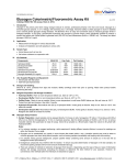
location on your computer, if you selected a different location in the installation process. By doubleclicking on the "Dizzy" symbolic link, the Dizzy program should start up. You should see an application
window appear that looks like the following picture:
file:///Volumes/Denali/Work/Old_Projects/Dizzy/UserManual/docs/UserManual.html
Page 5 of 49
Dizzy User Manual
11/15/09 7:47 PM
To load a model definition file into Dizzy, select the "Open..." item from the "File" menu. This will
open a dialog box, as shown here:
In the "Please select a file to open" dialog box, navigate to the directory in which you installed Dizzy.
Then navigate into the "samples" subdirectory. The dialog box should look like this:
file:///Volumes/Denali/Work/Old_Projects/Dizzy/UserManual/docs/UserManual.html
Page 6 of 49
Dizzy User Manual
11/15/09 7:47 PM
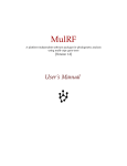
For starters, try selecting the "Michaelis.cmdl" file, by double-clicking on that file name in the dialog
box. The Dizzy window should now look like this:
Note that the model description has appeared in the editor window. In this window, you can edit a model
description, after which you may save your changes. You probably will not want to modify the
Michaelis.cmdl model definition file just yet. Note that the file name appears after the "file:" label.
There is also a label "parser:" label, whose function will be described later. Now, from the "Tools"
menu, select "Simulate...", which essentially processes the model definition and loads the relevant
information into the Dizzy simulation engine. This should create a "Dizzy: simulator" dialog box, that
looks like this:
file:///Volumes/Denali/Work/Old_Projects/Dizzy/UserManual/docs/UserManual.html
Page 7 of 49
Dizzy User Manual
11/15/09 7:47 PM
First, you will need to specify a "stop time" for the simulation. This is a floating-point number that you
must type into the text box next to the "stop time:" label in the "Dizzy: simulator" dialog box. Second,
you will need to select one or more species whose populations are to be returned as time-series data
resultant from the simulation. For the purposes of demonstration, select the "G3D_G80D" species in the
list box under the "view species" label in the dialog box.
TIP: You can select two species that are not adjacent to one another in the list box of
species, by holding down the "control" key, and (while holding down the key) clicking on a
species name with the mouse.
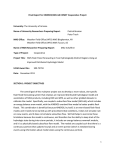
Finally, you will need to specify the "output type" for the simulation. For demonstration purposes, click
on the circular button next to the "plot" label on the dialog box. Go ahead and change the number of
samples to 30 samples, by editing the "100" appearing in the text box next to "num samples". This
controls the number of time points for which the result data will be graphed. At this point, the dialog box
should look like this:
Now, let's run the simulation, by single-clicking on the "start" button in the "Dizzy: simulator" dialog
box. After a moment, you should see a plot window appear that resembles the following image:
file:///Volumes/Denali/Work/Old_Projects/Dizzy/UserManual/docs/UserManual.html
Page 8 of 49
Dizzy User Manual
11/15/09 7:47 PM
For longer-running simulations, you can use the "cancel", "pause", and "resume" buttons to control a
running simulation. It is possible to pause and resume a simulation using the "pause" and "resume"
buttons. You may terminate a running simulation at any time using the "cancel" button. The "start"
button is only used to initiate a simulation. Only one simulation may be running at a time, in the Dizzy
application.
A special note applies to the case of importing a model definition file in SBML format, using the GUI
application. In this case, the GUI application will ask you to specify how species symbols appearing in
reaction rate expressions are to be interpreted. The choices given are "concentration" and "molecules". It
is recommended that you try using "concentration" first. If the GUI application complains that the initial
population of a given chemical species is too large for it to handle, try reloading the model with the
"molecules" choice instead. This will likely solve the problem.
Now that you have become acquainted with the simulation driver screen, the next step is to become
acquainted with the CMDL model definition language, which permits rapid development of new models.
To begin, let's define a simple model of a chemical system. This system will consist of the enzymesubstrate reaction:
E
S ---> P
where the "E" is the enzyme, and "S" is the substrate, and "P" is the product. It is well known that the
above symbols are shorthand for the following three elementary chemical reactions:
E + S ---> ES
ES
---> E + S
ES
---> E + P
where the "ES" species is the enzyme-substrate complex. We will now investigate the stochastic kinetics
of this very simple model using the Dizzy simulator.
A few notes about editing models: You may use the editor window in Dizzy, which is the white text box
below the "file:" and "parser:" labels, to enter the model description as described below. Once you have
entered the model description into the editor window, you may save the model description to a file by
selecting "save as" from the "File" menu. Alternatively, you use your own text editor program (e.g.,
Notepad on Windows) to create the model definition file. In that case, you would use the "open" menu
item under the "File" menu, to load the model definition file into Dizzy.
We will assume that the model definition file you are creating will be called "Model.cmdl". This file will
define the species and chemical reactions that make up the model, as well as the kinetic parameters that
file:///Volumes/Denali/Work/Old_Projects/Dizzy/UserManual/docs/UserManual.html
Page 9 of 49
Dizzy User Manual
11/15/09 7:47 PM
will be used to simulate the reaction kinetics. The ".cmdl" file extension is important, so please type the
file name exactly as shown. This helps the Dizzy program to recognize the file as an official "Dizzy
model definition file", and to select the proper interpreter to load the file. The file should start out
completely empty. Let's begin by defining the first of the three elementary reactions that make up the
above model. We will be defining this model in the CMDL language for entering a model definition file,
which is syntactically very close to the "Jarnac" language. At the top of the file, please enter the
following lines of text, exactly as shown here:
E = 100.0;
S = 100.0;
ES = 0.0;
r1, E + S -> ES, 1.0;
These lines are examples of statements. The first three statements define symbols "E", "S", and "ES",
and assign them the values 100.0, 100.0, and 0.0, respectively. The fourth statement is called a reaction
definition. These symbols represent initial species populations for the chemical species appearing in the
model. It is important that the reaction definition statement occurs after the statements defining the
species symbols that appear in the reaction. Since statements are processed sequentially by the Dizzy
parser, if the "ES = 0.0" statement did not occur before the reaction definition statement, the parser
would generate an error message because it would not recognize the "ES" symbol occurring in the
reaction definition statement. [At this point, processing of the model would cease because of the syntax
error.] You will notice that in the above example, each line ends with a semicolon. In the Dizzy
language, semicolons divide the model definition file into a sequence of statements. Each statement ends
with a semicolon. A statement can in principle extend over one line, as shown here:
r1, E + S -> ES,
1.0;
This definition is logically equivalent to the one-line reaction definition above it.
The commas in the reaction definition statement divide the statement into elements. We will explain
each element in turn. In a reaction definition statement, the first element is optional, and defines the
"name" of the reaction. This is just a symbolic name for the reaction, that does not affect the chemical
kinetics of the model. There are rules governing allowed symbol names that apply to reaction names.
The reaction name specified above was "r1", which is not very descriptive. Perhaps a more descriptive
name would have been "enzyme_substrate_combine", as shown here:
enzyme_substrate_combine, E + S -> ES, 1.0;
Note the use of the underscore character ("_"), which is necessary because spaces are not allowed in
symbol names such as reaction names. The second element of the reaction definition statement defines
the list of reactant species and products species for the chemical reaction. In this case, the reactants are
species "E" (the enzyme) and species "S" (the substrate). The special symbol "->" separates the list of
reactants and products. The sole product species is "ES", the enzyme-substrate complex. The "+"
operator is used to separate species in either the reactant or product side of the reaction. In passing, we
note that this is a one-way reaction, meaning that it defines a process that is not (by itself) reversible. To
define a reversible reaction in Dizzy, you would need to follow the above reaction definition statement
with a second reaction definition statement, in which the reactants and products are reversed, for
example:
enzyme_substrate_separate, ES -> E + S, 0.1;
The third element is a reaction rate. This can be specified as a bare number, a mathematical expression,
or as a bracketed mathematical expression. When you specify the reaction rate as a bare number or as an
(unbracketed) mathematical expression, you are instructing the Dizzy simulator to compute the reaction
rate using its built-in combinatoric method. This means that the reaction probability density (usually
designated with the symbol "a") per unit time is computed as the product of the number of district
combinations of reactant species, times the reaction rate parameter you specified in the reaction
definition. Let us illustrate this with an example. For the reaction
r1, A + B -> C + D, 2.0;
If species A has a population of 10, and species B has a population of 10, the reaction probability density
per unit time will be evaluated as the number of distinct combinations of reactant molecules (in this
case, that is 100) times the reaction rate parameter, 2.0. The resulting reaction probability density per
unit time will be 200. This probability density can be used to compute the probability P that a given
chemical reaction will occur during an infinitesimal time interval dt:
file:///Volumes/Denali/Work/Old_Projects/Dizzy/UserManual/docs/UserManual.html
Page 10 of 49
Dizzy User Manual
11/15/09 7:47 PM
P = a dt
The probability that a given chemical reaction (whose probability density per unit time is designated
with the symbol "a") will occur during the infitesimal time interval dt is just the product of the
infinitesimal time interval, and the reaction probability density per unit time.
An example of a reaction definition with a mathematical expression for the reaction rate is shown here:
A =
B =
C =
D =
F =
G =
r1,
100.0;
100.0;
0.0;
0.0;
10.0;
10.0;
A + B -> C + D, F * G;
In the above example, the parser will attempt to immediately evaluate the expression "F * G". This
evaluation will yield the result "100.0". Therefore, the above is functionally equivalent to:
A =
B =
C =
D =
r1,
100.0;
100.0;
0.0;
0.0;
A + B -> C + D, 100.0;
In either case, the built-in combinatoric method for computing the reaction rate is used, with a reaction
parameter of 100.0. For some cases, it may be desirable to specify a custom reaction rate, in which you
specify a mathematical expression that is to be re-evaluated for each reaction event, to give the reaction
rate. This might be useful for simulating cooperativity, or enzyme reactions, or inhibition. An example
of a reaction defintion with a custom reaction rate expression is shown here:
A =
B =
C =
D =
k =
r1,
100.0;
100.0;
0.0;
0.0;
0.1;
A + B -> C + D, [k * (time + 1.0) * A * B];
The symbol "time" is a special reserved symbol indicating the elapsed time of the simulation.
Getting back to our previous model-building exercise, we have:
E = 100.0;
S = 100.0;
ES = 0.0;
enzyme_substrate_combine, E + S -> ES, 1.0;
enzyme_substrate_separate, ES -> E + S, 0.1;
we see that the forward reaction for the enzyme and substrate combining, was given a reaction rate
parameter of 1.0, and the reverse of that reaction (enzyme-substrate complex separating) was given the
rate of 0.1.
Note that in defining a chemical reaction, the element specifying the reaction name is not required. If
you do not specify a reaction name, a unique reaction name is automatically assigned to the reaction by
Dizzy. The syntax for a reaction thus defined is:
A + B -> C + D, 2.0;
It is recommended that you specify your own reaction names, because the names automatically assigned
by Dizzy will be verbose and hard to understand.
Now, let's define the third reaction, which takes the enzyme-substrate complex to the enzyme plus
product,
make_product, ES -> E + P, 0.01;
file:///Volumes/Denali/Work/Old_Projects/Dizzy/UserManual/docs/UserManual.html
Page 11 of 49
Dizzy User Manual
11/15/09 7:47 PM
We will also need to define the initial population of the "P" species, using the statement:
P = 0.0;
(note that this statement must occur before the "make_product" reaction definition statement occurs in
the model definition file). Putting the three reaction definition statements together, your model definition
file should look like this:
E = 100.0;
S = 100.0;
P = 0.0;
ES = 0.0;
enzyme_substrate_combine, E + S -> ES, 1.0;
enzyme_substrate_separate, ES -> E + S, 0.1;
make_product, ES -> E + P, 0.01;
The Dizzy system ignores whitespace that is not in a quoted string, so you may reformat your model
definition file using spaces, so that it is more tabular:
E = 100.0;
S = 100.0;
P = 0.0;
ES = 0.0;
enzyme_substrate_combine,
enzyme_substrate_separate,
make_product,
E + S -> ES,
ES
-> E + S,
ES
-> E + P,
1.0;
0.1;
0.01;
Note that it is very important that the statements defining the initial species populations appear before
the reaction definition statements. Otherwise, the Dizzy interpreter will not understand the species
symbols appearing in the reaction definition.
The final model definition file should look like this:
E = 100;
S = 100;
P = 0;
ES = 0;
enzyme_substrate_combine,
enzyme_substrate_separate,
make_product,
E + S -> ES,
ES
-> E + S,
ES
-> E + P,
1.0;
0.1;
0.01;
Remember, whitespace is ignored by the Dizzy interpreter, so your spacing does not need to look
exactly like the example shown above. Now, let's save this model definition file in your text editor.
Now, let's open the model definition file in Dizzy, as shown above. Finally, let's select the "Simulate..."
menu item from the "Tools" menu, and run a simulation. Select a stop time of 400.0, and specify an
output type of "plot", and a "num samples" of 40. Select "P" as the species to view. Your simulation
controller dialog box should look like this:
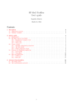
Now, run the simulation. You should see the familiar Michaelis-Menten type reaction kinetics appear in
a plot window:
file:///Volumes/Denali/Work/Old_Projects/Dizzy/UserManual/docs/UserManual.html
Page 12 of 49
Dizzy User Manual
11/15/09 7:47 PM
Note that the curve is not a perfect Michaelis-Menten kinetics. This is because we are running a
stochastic simulation. The Gillespie algorithm introduces the noisy effects of low copy numbers of
chemical species in the model. If we were to drastically increase the number of species (say, by a factor
or 1000) in the model, the curve would become less noisy:
Note that the larger the initial copy number of the species in the model, the more computational time
will be requird to simulate the model for a given (fixed) choice of "stop time". This means that in
general, when running stochastic simulations you should start with small initial copy numbers for the
species in your model, and determine the computational run-time, before attempting simulations with
large initial species populations.
Sample Model Definition Files
file:///Volumes/Denali/Work/Old_Projects/Dizzy/UserManual/docs/UserManual.html
Page 13 of 49
Dizzy User Manual
11/15/09 7:47 PM
When you install the Dizzy application, a subdirectory "samples" is created in the directory where Dizzy
is installed. You will find examples of all three languages in the "samples" subdirectory of the directory
in which you install the Dizzy software.
Note to Windows users: please do not use Notepad to open the sample model definition
files in the "samples" subdirectory. Please use a different editor, such as WordPad or
Emacs, in order to ensure that the files appear properly formatted, in the editor. You may
wish to associate ".cmdl" and ".dizzy" files with the WordPad program, so that you
can double-click on a ".cmdl" or ".dizzy" file and have it open (properly formatted)
in WordPad.
In addition, there is a repository of biomolecular models maintained by the CompBio Group, that will
serve as a good source of sample model definition files.
Preliminary Concepts
This section describes preliminary concepts that are common throughout the various model definition
languages for the Dizzy system.
Numeric Precision
All floating-point numbers in the Dizzy system are Java double-precision numbers. This means that they
are floating-point numbers in a 64-bit representation adhering to the IEEE 754-1985 standard. Java
double-precision floating-point numbers provide approximately 15 digits of precision. All internal
calculations are performed using double-precision floating-point arithmetic, unless otherwise noted.
It should be noted that the above limitation of the number of significant digits of a double-precision
floating-point number in Java, means that reaction rates differing by more than 15 orders of magnitude
will cause incorrect results from the stochastic simulator. In practice, this limitation rarely presents a
problem.
Another consequence of numeric precision is that a model containing a dynamical species whose initial
population is greater than or equal to 9.0071993e+15 molecules will not be allowed to be simulated
using a stochastic simulator. In addition, if the value of any dynamical species becomes greater than the
aforementioned threshold during the course of a simulation, an error message will occur, and the
simulation will be terminated. This is because the number of molecules is stored using a doubleprecision floating-point number, and for numbers greater than the aforementioned value, there are not
enough significant digits in the floating-point representation to account for an increment or decrement of
the species population by one molecule.
Case Sensitivity
All symbols, keywords and expressions in the Dizzy system are case-sensitive. This means that if you
define a symbol such as "x" (lower-case), you cannot later refer to it as "X" (upper-case). Similarly,
mixed-case keywords that are built into the Dizzy system, such as the keyword exportModelInstance,
must be entered exactly as shown; case variants such as exportmodelinstance would not be
recognized as valid keywords.
Symbol Names
Symbol names are a core ingredient of the Dizzy system. Most elements of the Dizzy system (reactions,
species, parameters, compartments, etc.) are named elements whose names must be valid symbol names.
A symbol name must conform to the following rules:
1. A symbol name must be composed entirely of alphanumeric characters, and the underscore
character. It may not start with an underscore character.
2. A symbol name must not parse as a numeric literal (i.e., it cannot be a number, such as 32
3. A symbol name may not start with the first character being a numeric character (0-9)
4. the symbols time and Navo are reserved, because they represent clock time and Avogadro's
constant, respectively
Note that Rule #1 above implies that a symbol name cannot contain parentheses, square brackets, curly
braces, or the arithmetic operators: +, -, *, /, %, ^, or the relations >, <, and =. Further, it implies that a
symbol name cannot contain the following reserved characters: !, @, #, $, |, &, ;, =, the comma ",", and
the period ".".
file:///Volumes/Denali/Work/Old_Projects/Dizzy/UserManual/docs/UserManual.html
Page 14 of 49
Dizzy User Manual
11/15/09 7:47 PM
For the reader who is familiar with the C programming language, the above can be summarized as: a
symbol name is legal if it would be a legal variable name in a C program.
Some examples of valid symbol names are shown here:
Species_A
Galactose
DNA_plus_TFA
P1
The following shows some examples of illegal symbol names:
ILLEGAL:
A + B
DNA plus TFA
C-D
1.0
1e+6
B!
The underscore can be used as a convenient separator when defining a symbol name with multiple
words.
Symbol names are stored in a namespace. There are two types of namespaces, global and local.
Normally, all symbol names reside in the global namespace. This applies to species names, reaction
names, compartment names, and parameter names. This means that you cannot define a species X and a
reaction X; their names would collide in the global namespace.
The local namespace applies only to a parameter that is defined only for a specific reaction (or
reactions). Each reaction has a local namespace for its reaction-specific parameters. It is permissible to
define a parameter X in the global namespace, and to also define a parameter X with a different value, in
the local namespace for one or more reactions. In that case, the value associated with X for the specific
reaction supersedes the value associated with X in the global namespace, for the purpose of evaluating
the custom reaction rate expression for the reaction. This can be summarized by saying that a parameter
defined locally supersedes a parameter defined globally, of the same name. The local namespace concept
applies only to parameters. Note that defining parameters within the local namespace is not possible in
the Chemical Model Definition Language.
Mathematical Expressions
Various aspects of the Dizzy system permit the textual specification of mathematical expressions. This is
a useful method of customizing reaction rate equations and other aspects of a chemical system model. A
mathematical expression may involve symbols, numeric literals, arithmetic operators, and built-in
mathematical functions.
Symbols are analogous to algebraic variables or symbols. Depending on the context, a symbol may
represent the population or concentration of a chemical species, or it may represent a floating point
parameter defined for a model or a chemical reaction. In the context of an expression, a symbol always
has an associated numeric value. When a symbol appears in a mathematical expression, its associated
numeric value is used in place of the symbol, for the purpose of evaluating the expression.
In the context of a mathematical expression, numeric literals are simply numbers, either floating point or
integer. Note that within a mathematical expression one may use scientific notation (e.g., 1.2e-7 or
1.2e+7) to specify floating-point numeric literals. Alternatively, one may use constructions such as
1.2*10^7 and 1.2*10^(-7) to represent floating-point numeric literals (but in deferred-evaluation
expressions, the latter method is less efficient than scientific notation using the "e" character shown
above).
In the Dizzy system, mathematical expressions are described using a syntax similar to the C
programming language. The basic operations permitted are:
addition
adding two symbols, numbers, or sub-expressions, such as A+B, or A+1.7, or 2+2
subtraction
computes the difference of two symbols, numbers, or sub-expressions, such as A-B, or
A-1.7, or 2-2
file:///Volumes/Denali/Work/Old_Projects/Dizzy/UserManual/docs/UserManual.html
Page 15 of 49
Dizzy User Manual
11/15/09 7:47 PM
multiplication
multiplying two symbols, numbers, or sub-expressions, such as A*B, or A*1.7, or 2*2
division
computes the quotient of two symbols, numbers, or sub-expressions, such as A/B, or
A/1.7, or 2/2. The first operand is the dividend, and the second operator is the
divisor.
modulo division
computes the remainder of the quotient of two symbols, numbers, or sub-expressions,
such as A%B, or A%1.7, or 2%2. The first operand is the dividend, and the second
operator is the divisor.
exponentiation
computes the exponent of two symbols, numbers, or sub-expressions, such as A^B, or
A^1.7, or 2^2. The first operand is the value being exponentiated. The second operand
is the exponent.
parentheses
represents a sub-expression whose value is to be computed, such as the subexpression (B+C) appearing in the expression A+(B+C).
negation
computes the negative of a symbol, number, or sub-expression, such as -A, or -1.0,
or -(A+B).
In addition to the above operations, there are a number of built-in mathematical functions that may be
used in mathematical expressions. Unless otherwise stated, the built-in functions described below are
implemented by calling the corresponding function in the java.lang.Math class in the Java Runtime
Environment. The built-in mathematical functions available for use in mathematical expressions are:
exp
Computes the value of the base of the natural logarithm, e, raised to the power of the
(floating-point) argument.
ln
Computes the natual logarithm of the argument, which must be in the range (0,
infinity).
sin
Computes the trigonometric sine of the argument. The argument is an angle, which
must be specified in radians. Example: sin(A), sin(3.14159).
cos
Computes the trigonometric cosine of the argument. The argument is an angle, which
must be specified in radians. Example: cos(A), cos(3.14159).
tan
Computes the trigonometric tangent of the argument. The argument is an angle, which
must be specified in radians. Example: tan(A), tan(3.14159).
asin
Computes the trigonometric inverse sine of the argument. The argument is a
dimensionless ratio, that must be within the range [-1,1]. The value returned is an
angle, in radians. Example: asin(A), asin(0.5).
acos
Computes the trigonometric inverse cosine of the argument. The argument is a
dimensionless ratio, that must be within the range [-1,1]. The value returned is an
angle, in radians. Example: acos(A), acos(0.5).
atan
Computes the trigonometric inverse tangent of the argument. The argument is a
dimensionless ratio. The value returned is an angle, in radians. Example: atan(A),
acos(0.5).
abs
Computes the absolute value of the argument.
floor
Computes greatest integer value that is less than or equal to the floating-point
argument. Example: floor(A), floor(1.7)
ceil
Computes the smallest integer value that is greater than or equal to the floating-point
argument. Example: ceil(A), ceil(1.7)
sqrt
Computes the value of the square root of the argument. The argument must be
nonnegative.
theta
file:///Volumes/Denali/Work/Old_Projects/Dizzy/UserManual/docs/UserManual.html
Page 16 of 49
Dizzy User Manual
11/15/09 7:47 PM
Returns 0.0 if the argument is negative, or 1.0 if the argument is nonnegative (i.e.,
zero or positive)
min(X,Y)
Returns the smaller of expressions X and Y. This is a two-argument function.
max(X,Y)
Returns the larger of expressions X and Y. This is a two-argument function.
New built-in mathematical functions may be added in forthcoming versions of the Dizzy system.
Please remember that all elements of the Dizzy system are case-sensitive, including the aforementioned
built-in mathematical functions. Therefore an expression such as SIN(3.14) would not be recognized as
referring to the sin trigonometric function. The expression would therefore be considered invalid,
because the SIN function would not be recognized as a valid built-in function.
It is important to note that all expressions are evaluated using double-precision floating-point arithmetic.
For functions that return an integer, such as the floor() function appearing in the expression A *
floor(B), the integer result of floor(B) is converted to a double-precision floating-point number,
before the result is used in evaluating the A * floor(B) expression.
The following are a few examples of valid mathematical expressions that have been used in Dizzy
models:
10*(1/(1+exp(-0.0025*(-2000+time))))
alpha0 + (alpha + PY^n*alpha1)/(K^n + PY^n)
k * (A/(N*V)) * (B/(N*V))
Note that the symbols time and N are special symbols, defined above.
Certain functions offered above, are not differentiable. This means that algorithms or features of Dizzy
that rely on the Jacobian matrix of the model (the partial derivative of the time rate of change of the ith
species in the model, with respect to the jth species), may not be used if you specify a model that
contains one of these non-differentiable functions in an expression. An error will result if you attempt to
use a feature that relies on the Jacobian, with a model containing a non-differentiable function. The nondifferentiable functions are: theta(), ceil(), floor(), abs(), and the modulo division operator %. The
features in Dizzy that rely on the Jacobian are the Tau-Leap simulators and the steady state fluctuations
estimator (the latter relies on the Jacobian only in the case of an ODE-based simulator).
When specifying a mathematical expression, it is important to understand the distinction between
immediate evaluation and deferred evaluation. An example of immediate evaluation is shown here:
A = 1.0;
B = A * 5.0;
The value for the symbol B is set to 5.0. The mathematical expression appearing in the definition of
symbol B is immediately evaluated by the parser, so any symbols appearing in that expression (namely,
A) must have been previously defined as symbols in the model. The special symbols "time" and "Navo"
may not be used in immediate-evaluation expressions.
An example of deferred evaluation is shown her:
A = 1.0;
B = [A * 5.0];
The square brackets define the expression as a deferred-evaluation expression. This means that the
parser stores the expression and associates it with the symbol B, rather than a value. The expression will
be evaluated by the simulation engine only when a value for the symbol "B" is needed. The special
symbols "time" and "Navo" may be used in deferred-evaluation expressions.
Important note about time-dependent expressions:
Although it is technically possible to define a rate law or other expression that has an explicit time
dependence through the use of the reserved symbol "time", this practice is discouraged when using the
stochastic simulators. This is because the stochastic simulators are based on a mathematical theory of
file:///Volumes/Denali/Work/Old_Projects/Dizzy/UserManual/docs/UserManual.html
Page 17 of 49
Dizzy User Manual
11/15/09 7:47 PM
reaction kinetics in which the time-invariance of the reaction parameters is a priori assumed. The time
reserved symbol is intended solely for use with the ODE simulators. A very slowly-varying time
dependence for some expression in a model, may be compatible with the stochastic simulators, to the
extent that on the time scale for any reaction to occur, the expression is effectively time-translationinvariant.
Gillespie Stochastic Algorithm
The Gillespie stochastic algorithm is an algorithm for modeling the kinetics of a set of coupled chemical
reactions, taking into account stochastic effects from low copy numbers of the chemical species. The
algorithm is defined in the article:
D. T. Gillespie, "A General Method for Numerically Simulating the Stochastic Time
Evolution of Coupled Chemical Species", J. Comp. Phys. 22, 403-434 (1976).
In Gillespie's approach, chemical reaction kinetics are modeled as a markov process in which reactions
occur at specific instants of time defining intervals that are Poisson-distributed, with a mean reaction
time interval that is recomputed after each chemical reaction occurs. For each chemical reaction interval,
a specific chemical reaction occurs, randomly selected from the set of all possible reactions with a
weight given by the individual reaction rates.
The Dizzy system provides a Java implementation of the Gillespie algorithm, for which more
information is available in the Javadoc documentation. This implementation uses the "direct method"
variant of Gillespie's algorithm.
Gillespie Tau-Leap Stochastic Algorithm
The Gillespie Tau-Leap algorithm is a method for obtaining approximate solutions for the stochastic
kinetics of a coupled set of chemical reactions. An dimensionless relative tolerance "epsilon" controls
the amount of error (as compared to the Gillespie Direct method) permitted in the solution, by scaling
the maximum allowed "leap time" which is recomputed after each iteration of the algorithm. The leap
time is the amount by which the time is stepped forward during the iteration. The number of times each
reaction in the model occured during the leap time is computed as the result of a Poisson stochastic
process. Species populations are adjusted in accordance with the number of times each reaction occurred
during the leap time interval. In the limit as the epsilon parameter is set to zero, the Tau-Leap algorithm
should agree precisely with the results of the Gillespie Direct algorithm. For complex models with a
significant separation of time scales, this algorithm may potentially be much faster than the Gillespie
Direct algorithm.
The Tau-Leap algorithm is described in:
D. T. Gillespie and L. R. Petzold, "Improved Leap-Size Selection for Accelerated
Stochastic Simulation", J. Chem. Phys. 119, 8229-8234 (2003).
and in references therein.
Two implementations of the Tau-Leap algorithm are provided with Dizzy The first is called "tauleapsimple". It is intended for use with models that are entirely composed of elementary reactions, that is,
reactions with rate laws that are simple mass-action kinetics. The second is called "tauleap-complex".
It is intended for use with models that contain custom algebraic rate expressions.
Gibson-Bruck Stochastic Algorithm
The Gibson-Bruck stochastic algorithm is an algorithm for modeling the kinetics of a coupled set of
coupled chemical reactions. The algorithm is defined in the article:
M. A. Gibson and J. Bruck, "Efficient Exact Stochastic Simulation of Chemical Systems
with Many Species and Many Channels", Caltech Parallel and Distributed Systems Group
technical report number 026, (1999).
This implementation uses the "next reaction" variant of the Gibson and Bruck algorithm, for which
more information is available. The Gibson-Bruck algorithm is O(log(M)) in the number of reactions, so
it is preferred over the Gillespie algorithm for models with a large number of reactions and/or species.
file:///Volumes/Denali/Work/Old_Projects/Dizzy/UserManual/docs/UserManual.html
Page 18 of 49
Dizzy User Manual
11/15/09 7:47 PM
For models with a small number of reactions and species, the Gillepie algorithm is preferred, as it avoids
the overhead of maintaining the complex data structures needed for the Gibson-Bruck algorithm.
Deterministic simulation using ODEs
The Dizzy system provides several simulators for approximately solving the deterministic dynamics of a
model as a system of ordinary differential equations (ODEs). A differential equation, called a rate
equation, is generated expressing the time rate of change of the concentration of each chemical species
in the model. This coupled set of differential equations is solved using finite difference techniques. The
simplest methods use a fixed time-step size. More sophisticated methods use a variable time-step size
that is controlled by an adaptive method involving a formula for estimating the error. If the error gets too
large, the time-step size is decreased until the error is acceptable. If the error becomes very small, the
time-step size is increased (to improve speed) as much as possible without exceeding the allowed error.
Each step involves computing the concentration of all species at the next time step, using a finite
differencing sheme. Several categories of finite differencing schemes exist. The explicit schemes
compute the concentration at the next time-step using only derivatives at the previous time-step. The
implicit schemes compute the concentration at the next time-step using only derivative values from the
next time-step; these methods involve solving a (usually nonlinear) implicit equation for the
concentration at the next time-step, for each iteration. A linearly implicit or implicit-explicit scheme is
a compromise where the linear term is treated using an implicit method, and the nonlinear term is
treated using an explicit method. This ensures that at most a linear system of equations needs to be
solved for each iteration. For more information, please see the book
Introduction to Numerical Analysis, Second Edition, by J. Stoer and R. Bulirsch. New
York: Springer-Verlag, 1993.
The deterministic simulators are approximate for two reasons. First, they are solving a set of ordinary
differential equations that are themselves an approximation to the underlying stochastic kinetics of the
system. Second, they are using finite-difference methods that usually only give an approximate
numerical solution to a system of differential equations. However, the deterministic simulators have the
advantage of usually being much faster than the stochastic simulators, for most models. This means that
they can be very beneficial in situations where rapid model solution is required, such as multi-parameter
optimization of a model.
Model Elements
Parameters
A parameter is a name-value pair that may be referenced symbolically (i.e., by its name) in mathematical
expressions. The value is always a numeric (floating-point) value. The parameter name must be a valid
symbol name.
A parameter can be associated with a model, in which case it can be referenced in the custom rate
expression for any chemical reaction associated with the model; in addition, it can be referenced in the
species population expression for any boundary species within the model.
Compartments
A compartment is an abstraction for a named region of space that has a fixed volume. The contents of
this volume are assumed to be well-stirred, so that chemical species do not have concentration gradients
within this volume. Every species must be assigned to a compartment. The volume of the compartment
can be used to compute the concentration of the species, from the number of molecules (population) of
the species in the compartment.
By default, species defined in the Chemical Model Definition Language are associated with a default
compartment "univ" This compartment has unit volume.
A non-default compartment can be defined by a symbol definition as shown here:
c1 = 1.0;
A species "S" can be associated with this compartment by the statement:
S @ c1;
file:///Volumes/Denali/Work/Old_Projects/Dizzy/UserManual/docs/UserManual.html
Page 19 of 49
Dizzy User Manual
11/15/09 7:47 PM
The special symbol "@" is used to associate a species with a compartment. Note that the species symbol
"S" and the compartment symbol "c1" must have been previously defined, as shown here:
c1 = 1.0;
S = 100.0;
S @ c1;
The above statement would tell the parser to define the two symbols "S" and "c1" with values 100 and 1,
respectively, and that "S" is a species associated with the compartment "c1".
Species
A species is an abstraction representing a type of molecule or molecular state. A species has a name,
which must be unique; in addition, a species must be assigned to one (and only one) compartment. A
species must also be assigned a population value, which is a double-precision floating point number.
There are two types of species in the Dizzy system, dynamical species and boundary species.
A dynamical species (called a "floating" species in SBML) is a species whose population is affected by
reactions in which it participates. For example, if a reaction takes species X as a reactant, and does not
produce species X as a product, then when this reaction occurs, the population of species X is
decremented by one. The dynamical species is the most commonly used species type, and it is the
default species type for species in the Dizzy system.
A boundary species is a species whose population is externally specified as a boundary condition for the
simulation. The population of a boundary species is not affected by the occurrence of reactions in which
the species participates. In this sense, a boundary species is not "dynamical". The population of a
boundary species can be set to a constant, or a more complex time-dependent function. The details of
how to define the population of a boundary species will be discussed further below.
Occasionally it is desirable to create a model in which a given species can reside in more than one
compartment. This is accomplished in the Dizzy system by defining two different species with similar
(but still distinct) names, and assigning each species to a different compartment. For example, one
might define two different species named "SpeciesX_cytoplasm" and "SpeciesX_nucleus",
representing the instances of chemical species "X" in the cytoplasm and nucleus, respectively.
Please note that there is a restriction on the initial population that can be specified for dynamical
species. This particular limitation only affects stochastic simulations.
Reactions
A reaction is a one-way process in which zero or more chemical species may interact, transforming into
zero or more (possibly different) chemical species. The interacting species are the reactants, and the
chemical species that are produced are called the products.
Here, "one-way" means that a single reaction defines a process that can only proceed from reactants to
products. The "reverse" reaction is not implicitly defined. In order to model a chemical system with a
"reversible" reaction, a second reaction must be defined in which the roles of reactants and products are
swapped.
The mention of "zero species" above merits some explanation. Consider the case of a chemical reaction
with zero reactants and a finite number of products. This represents a process in which the products are
spontaneously created, somewhat like pair creation of an electron-positron pair from the vacuum, in the
presence of a strong electic field. The case of zero products and a finite number of reactants represents a
process of annihilation of the reactant molecules, such as in electron-positron pair annihilation. Note that
a reaction with zero reactants and zero products is not permitted by the Dizzy system. The cases of zero
reactants or zero products are somewhat degenerate, but are useful for defining a signal molecule with
an (ensemble-averaged) equilibrium population that is a time-dependent function. For example, one can
model a signal molecule "S" whose equilibrium population is a specified function of time by considering
two separate
It is permissible for a chemical species to participate in a reaction as both a reactant and a product, as
shown here:
A + B -> A + C
In such a reaction, a single molecules of species A is used in the reaction, but also produced, so the net
file:///Volumes/Denali/Work/Old_Projects/Dizzy/UserManual/docs/UserManual.html
Page 20 of 49
Dizzy User Manual
11/15/09 7:47 PM
change in the population of species A from this reaction is zero. Note that the above reaction definition
is not a good model of catalysis. A simple model of catalysis in which species A catalyzes the
transformation of species B into species C would involve three separate reactions, as shown here:
A + B -> AB
AB -> A + B
AB -> A + C
with appropriate conditions on the relative rates of the second and third reactions. Note that the species
named "AB" represents the enzyme-substrate complex.
The above discussion assumes that species participating in reactions are dynamical species. As described
above in the species section, a species can also be defined as a "boundary" species. In this case, the
population of the species is not dynamical but instead a boundary condition of the system. As an
illustration, suppose that species X is declared as a boundary species. Even if species X were to appear in
a reaction as a reactant, such as in the reaction X + A -> B, the population of species X would not be
affected by the occurrence of this reaction. This is mostly useful for defining a species whose role in a
system is as an externally applied "signal" or "input". Note that special notation is used to describe a
boundary species in the Chemical Model Definition Language (CMDL), as described below.
Reaction Rates
A reaction rate is defined as the probability density per unit time, of a given chemical reaction occurring.
In the Dizzy system, there are two methods of defining reaction rates, the built-in method and the
custom expression method. The built-in method is the default method used, and it is preferred for
reasions of computational performance (speed).
In the built-in method of defining a reaction rate, one specifies a numeric reaction parameter. The
units of the reaction parameter depend on the reaction rate species mode attribute of the model with
which the reaction is associated.
If the model's reaction rate species mode is molecules (the default), the reaction parameter represents the
numeric reaction probability density per unit time, per distinct combination of reactant molecules. The
reaction rate is then obtained by first computing the number of distinct combinations of reactant
molecules (which depends on the populations of the various reactant species), and multiplying this
number by the reaction parameter for the reaction. The result is the reaction rate.
If the model's reaction rate species mode is concentration, the reaction parameter represents the kinetic
constant for the reaction, in units of inverse molar concentration to the power of the number of reactant
species, per unit time. In this case, the concentration of each reactant species is computed, and the
concentrations are multiplied together (with suitable exponentiation for a reactant species that has a
stoichiometry greater than one). The result is then multiplied by the reaction parameter, to produce the
reaction rate.
In the custom expression method of defining a reaction rate, one specifies a textual reaction rate
expression. This expression is a mathematical expression involving symbols, arithmetic operators, and
simple built-in mathematical functions. Symbols can be species names or parameters. A species name
appearing in the expression represents either the number of molecules of the species, or the species
concentration, depending on the reaction rate species mode of the model with which the reaction is
associated. The custom expression method is less desirable than the built-in method, due to the
computational overhead of evaluating the mathematical expression for each reaction event during the
simulation of the model.
Multistep Reactions
The Dizzy system allows for defining an N-step process as a single composite "reaction". This is an
experimental feature that still needs further testing before it can be considered reliable. As a more
reliable and better-tested alternative, consider using the delayed reaction construct.
A multistep reaction assumed to consist of N irreversible elementary reactions that are chained together,
as shown here:
S0 -> S1 -> S2 -> S3 -> S4 -> ... -> SN
One should note that it is possible to define each of these reaction steps separately, as shown here:
file:///Volumes/Denali/Work/Old_Projects/Dizzy/UserManual/docs/UserManual.html
Page 21 of 49
Dizzy User Manual
11/15/09 7:47 PM
S0 -> S1, k; S1 -> S2, k; ...
The loop construct can make the above definition easier. However, if the following conditions are met:
1. each reaction step has precisely one reaction and one product
2. all the reactions have the same elementary rate value (which may not be a custom expression)
3. the reactions are chained together as shown above
it is possible to simplify the reaction definitions using a single "multistep" composite reaction:
S0 -> S1, k, steps: N;
where k is the rate value for each elementary reaction, and N is the number of reaction steps in the
composite multistep reaction. If the value specified for N is less than or equal to 15, the Dizzy simulator
will just insert the N separate reactions into the model. If the value N is greater than 15, the Dizzy
simulator will treat the cascade of reactions as a single "multistep" reaction, using a history-dependent
mechanism for evaluating the probability density of producing a molecule SN at any given time. This
method is described in the paper of Gibson and Bruck.
Multistep reactions are useful for simulating processes such as transcription and translation, in which a
long sequence of individual reaction steps transforms the system from an initial state ("polymerization
complex") to a final state ("completed transcript").
Delayed Reactions
The Dizzy system allows for defining a reaction process containing an intrinsic "delay". This can be
useful for phenomenologically modelling complex processes for which the detailed dynamics is not
known, but for which the overall rate is known and the total time for the process to occur, is known. A
delayed reaction must have exactly one reactant and one product species. The delayed reaction takes up
the reactant and produces the product molecule, at the specified rate. However, the rate of production of
the product species depends upon the number of reactant molecules at a time in the past equal to the
"delay" time specified for the reaction. For reactant S0 and product S1 and delay s and rate k, the
delayed reaction is equivalent to the following differential equations:
dS0/dt = -k * S0(t)
dS1/dt = k * S0(t - s)
To define a delayed reaction equivalent to the above, the command language statement would be:
S0 -> S1, k, delay: s;
where k is the rate value for each elementary reaction, and s is the delay. The delay time is in the same
units as the time scale used for all kinetic parameters in the model, and must be a nonnegative number.
Specifying a delay time of zero is equivalent to having no delay at all.
Models
In the Dizzy system, a model is a collection of one or more reactions, together with all of the chemical
species involved in the reactions, and any parameters defined for the model or the reactions. In addition,
a model contains all of the compartments with which the species are associated. A model also
incorporates the initial species populations.
A model has an important attribute called the reaction rate species mode. This attribute controls how a
given species contributes to a reaction rate. It has two possible values, molecules and concentration.
Each will be defined in turn.
In the molecules reaction rate species mode, the contribution of any given species to a reaction rate is
always computed using the number of molecules of the species. In the case of the default method of
computing the reaction rate, this means that the reaction rate is computed as the product of the number
of distinct combinations of reactant molecules, and the reaction parameter. The molecules reaction rate
species mode is the default.
In the concentration reaction rate species mode, the contribution of a given species to a reaction rate is
computed using the molar concentration of the species (number of moles of the species, divided by the
volume of the compartment).
file:///Volumes/Denali/Work/Old_Projects/Dizzy/UserManual/docs/UserManual.html
Page 22 of 49
Dizzy User Manual
11/15/09 7:47 PM
Chemical Model Definition Language (CMDL)
The Chemical Model Definition Language (CMDL) is a simplified model definition language designed
to minimize the amount of repetitive typing required to define a model. The default file extension of
model definition files in the CMDL language is the ".cmdl" suffix. The alternative extension ".dizzy"
is also understood to indicate a CMDL file.
Character Encoding
All CMDL files are required text files in UTF-8 encoding, which includes comments. This is to ensure
uniform behavior of the Dizzy parser on all platforms, regardless of the default character encoding used
in the particular locale. In particular, Red Hat Linux distributions subsequent to version 8, employ UTF8 encoding as the default character encoding; therefore, care must be used to avoid embedding nonUTF-8 characters within a CMDL file.
Symbol Values
A fundamental concept in the CMDL language is the symbol value. A symbol value is an assocation
between a symbol name and a value. A value may be defined as a mathematical expression, in which
case it is immediately evaluated and the resulting floating point value is associated with the symbol. Or,
the value may be defined as a bracketed mathematical expression (enclosed in square brackets), in
which case the expression itself is stored and associated with the symbol name. The former type of value
(immediately evaluated expression) is akin to a numeric macro. The latter type of value (expression with
deferred evaluation) is similar to a symbolic function definition in Mathematica.
As mentioned previously, symbol names must be unique. This means that you cannot use the same
symbol name for two different purposes. For example, it is illegal to define both a species "S" and a
compartment "S". All elements of the Dizzy system (reaction names, species names, compartment
names, and parameter names) live in the same "namespace", and so each element must have a globally
unique name.
In the CMDL, compartments, species, and parameters all start out as symbol value definitions like this:
S = 1.0;
In this example, "S" is the symbol name, and the value is 1.0. The Dizzy parser determines that a given
symbol name is a species, compartment, or parameter based on how the symbol is subsequently used.
For example, if the symbol "S" appears as a reactant in a subsequent reaction definition,
r1, A + S -> C + D, 1.0;
the symbol "S" is automatically promoted to be a species. It cannot be subsequently used as a
compartment or other type of symbol. For the case of a compartment, suppose that a symbol "comp" is
defined as shown here:
comp = 2.0;
If this is later followed by a statement such as:
S @ comp;
the parser will automatically promote the symbol "comp" to be a compartment (and "S" will be
promoted to be a species, if this has not already happened). If at the end of processing all statements in
the model definition file, there are symbols left that are neither species nor compartments, these symbols
are added to the model as global parameters.
Statements
The CMDL langauge is centered around the concept of a statement. Model definition files are broken
into statements by use of the reserved symbol ";", the semicolon. Each statement must terminate with a
semicolon, even if there is only one statement in the file. The CMDL model definition file is tokenized
and parsed by the parser, and turned into an ordered collection of statements that are executed by the
scripting engine. In this way, there is a logical decoupling between parsing of model definition files and
the execution of the statements defining the model. Statements are processed in the order in which they
appear in a model definition file.
file:///Volumes/Denali/Work/Old_Projects/Dizzy/UserManual/docs/UserManual.html
Page 23 of 49
Dizzy User Manual
11/15/09 7:47 PM
There are two types of statements, known as statement categories. The first and most important
category of statements is known as model definition statements. This category of statements includes
all statements that define model elements, such as species, reactions, parameters, etc.
The second category of statements is known as action performers. These statements instruct the
scripting engine to perform a concrete action, such as conducting a simulation, exporting a model
definition, printing the contents of a data structure, etc. This category of statements is supported only for
use with the command-line interface to the Dizzy system. The graphical user interface for the Dizzy
system allows only the model definition statement category, and ignores any statements in the "action
performers" category. This is because in the graphical user interface, various graphical elements (menu
items, dialog boxes, and other controls) are used to instruct the application to perform actions, rather
than the scripting language.
File Inclusion
In the Dizzy system, a model definition file may include another model definition file. This include
mechanism is permitted in both of the command-language-based model definition language. Model
definitino file inclusion works just as it does with the preprocessor in the C programming language. The
parser splices the text of the included file into the including file, at exactly the point where the "include
directive" occurs. There is a built-in mechanism to prevent cyclic inclusion of files. If file A includes file
B, and file B includes file A, then the parser will simply ignore the include directive inside file B, since it
will already have processed file A.
The include mechanism is useful for separating out "boilerplate" macro definitions thare are shared from
model to model. In addition, the include mechanism might potentially be useful for extending a model.
The specific syntax for including a model definition file within another model definition file, is shown
here:
#include "myFile.cmdl";
where "myFile.cmdl" is the name of the file that is to be "included". The contents of "myFile.cmdl"
are parsed at exactly the point where the include statement is encountered in the file, after all statements
in the including file preceding the include statement have been parsed. Note that the double-quotes and
the semicolon are required. It is not allowed to embed a file inclusion statement inside a loop construct.
Normally, file includes are placed at the top of a model definition file, in order to load a separate file
containing "boilerplate" macro definitions and reaction definitions that are shared between different
models.
Comments
The CMDL provides a mechanism for embedding explanatory comments in a model definition file. A
comment is a fragment of text beginning with a double-slash ("//"). All text from the double-slash, to
the end of the line, are considered by the parser to be a comment, and are ignored. The following
example shows an example of a comment:
// this is a comment
It is acceptable to include a comment on the same line as an actual statement, as shown here:
<some statement>;
// this is a comment
In the above example, the statement would be parsed, but everything after (and including) the doubleslash would be ignored.
The Dizzy system also supports multi-line comments. The syntax for a multi-line comment is identical to
a comment in the C programming language:
/*
this is a comment
this is also a comment
*/
The parser will ignore anything between the "/*" and the "*/" symbols. This can be useful for
temporarily commenting out multiple lines of your model definition file, as shown here:
file:///Volumes/Denali/Work/Old_Projects/Dizzy/UserManual/docs/UserManual.html
Page 24 of 49
Dizzy User Manual
11/15/09 7:47 PM
/*
commented out temporarily for testing purposes (sramsey 2003/05/09)
G4_dimer_binding_at_DNA4,
G4D_free + DNA4 -> G4D_DNA4,
kf;
G4_dimer_debinding_at_DNA4,
G4D_DNA4 -> G4D_free + DNA4,
kr;
*/
Using the multiline comment syntax for this case is easier beacause you do not have to add a pound
symbol "//" to each line that you are commenting out.
Exporter Plug-ins
The Dizzy system has a framework of plug-ins for exporting an Dizzy model to different file formats.
Each exporter plug-in has an exporter alias defined. The default exporter is the exporter for Systems
Biology Markup Language (SBML). The SBML exporter has the exporter alias "markup-language"
(quotes not included). The full list of exporters is defined here:
markup-language
Exports a model instance to SBML.
human-readable
Exports a human-readable textual representation of the model.
orrell-column-format
Exports a model instance to a numeric-column-format used at Institute for Systems
Biology for certain software tools. Only models that do not contain any expressions
may be exported to this format.
command-language
Exports a model instance to the Chemical Model Definition Language (CMDL)
format.
Currently there is no exporter plug-in for the CMDL language. Additional exporter plug-ins may be
defined in the future.
Viewer Plug-Ins
The Dizzy system has a framework for pluggable model viewer modules. The viewer plugins are only
available in the graphical user interface to Dizzy A viewer is used to display a model, for example, a
graphical or textual representation on the screen. This is distinct from exporting the model to a different
file format. Each model viewer plug-in has an alias, which is a short texual name that identifies it. The
full list of model viewers is defined here:
cytoscape
Display the model in Cytoscape
human-readable
Display the model in human-readable format.
Simulator Plug-Ins
The Dizzy system has a framework for pluggable simulation modules. Each simulator plug-in has a
simulator "alias". The available simulator plug-ins are:
gillespie
An implementation of the Gillespie stochastic algorithm for modeling the reaction
kinetics. This algorithm is described in the article
ODE
An implementation of an ODE-based deterministic simulator of the reaction kinetics.
The implementation is based on a 5th-order Runge-Kutta integrator with an adaptive
stepsize controller.
Each simulator above is identified by its "simulator alias". For example, the simulator alias for the
Gillespie algorithm is "gillespie".
Default Model Elements
One of the distinguishing aspects of the CMDL is that several core elements are created by default:
A model is created, with model name "model". The model name can be modified with the
file:///Volumes/Denali/Work/Old_Projects/Dizzy/UserManual/docs/UserManual.html
Page 25 of 49
Dizzy User Manual
11/15/09 7:47 PM
"#model" statement.
A compartment is created, with name "univ" and volume of 1.0 liters
This provides a built-in "context" for reaction and species definitions. All species that are defined are
automatically associated with the default ("univ") compartment. All reactions are automatically
associated with the default model ("myModel").
The default "model" in the CMDL language has a reaction rate species mode of "molecules". In order to
use a reaction rate species mode of "concentration", it is presently necessary to use the programmatic
interface to Dizzy.
Reaction Statements
A CMDL model definition (usually, but not always, a single file) consists of a series of statements
which are text strings separated by semicolons. Whitespace and newlines are ignored by the CMDL
parser, except in a quoted string environment, where whitespace is interpreted literally and newlines are
illegal.
The centerpiece of the chemical model definition language is the reaction statement. A reaction
statement defines a one-way chemical reaction in which zero or more chemical species participate as
reactants, and zero or more chemical species participate as products. The species appearing in the
reaction definition must be previously defined symbols. Reaction statements have three elements
separated by commas. The first element is the reaction name, and it is an optional element. The second
element defines the reactants and products. The third element defines the reaction rate. The following
example shows a reaction statement, along with the preceding species symbol definitions:
A = 100.0;
B = 100.0;
C = 0.0;
D = 0.0;
creation_of_c_d,
A + B -> C + D,
1.0;
As explained above, each statement ends with the semicolon character ";". Note the use of the comma
character "," to separate different elements of the statement. The statement causes the following
definitions to be made:
a dynamical species A, in the default compartment
a dynamical species B, in the default compartment
a dynamical species C, in the default compartment
a dynamical species D, in the default compartment
a reaction creation_of_c_d, in which species A and B participate as reactants, and in which
species C and D are products.
the reaction rate of the creation_of_c_d reaction is computed using the built-in method, with a
reaction parameter of 1.0.
Please note that if the reaction name is omitted, the first comma must be omitted as well, as shown here:
A + B -> C + D,
1.0;
In this case, a default reaction name is assigned by the Dizzy parser.
In many cases, it is desirable to specify a custom reaction rate, rather than using the built-in method of
computing the reaction rate. To specify a custom reaction rate, the reaction rate element should be
defined as a string data type. This is accomplished by substituting a bracketed mathematical expression.
In the example of the above reaction, one might write:
creation_of_c_d,
A + B -> C + D,
[2.0 * A * B];
The square brackets are required in order to tell the parser that the reaction rate is a custom reaction rate,
for deferred (rather than immediate) evaluation. The text inside the quotes is parsed as a mathematical
expression that typically involves species name symbols, numeric literals, and arithmetic operators. In
addition, a mathematical expression may involve built-in functions (e.g., ln() or sin()) and special
symbols such as "time". In the above example, the reaction rate will be computed as the product of the
number 2.0 times the product of the populations of species A and B, in molecules.
file:///Volumes/Denali/Work/Old_Projects/Dizzy/UserManual/docs/UserManual.html
Page 26 of 49
Dizzy User Manual
11/15/09 7:47 PM
It should be emphasized that the CMDL parser determines which type of reaction rate computation
method to use, based on whether or not the reaction rate is specified using square brackets. As explained
above, if the rate expression is not bounded by square brackets, the parser will use the built-in reaction
rate computation method. If the rate expression is bounded by square brackets, the parser will assume
that the reaction rate computation method is a custom rate.
Note that specifying a custom reaction rate using a mathematical expression (in square brackets) has a
significant drawback, relative to using the built-in method of computing the reaction rate. The custom
reaction rate is more expensive to compute, in terms of the number of CPU instructions per reaction
event in the simulation.
Symbol Values and Expressions
Often, a single value will be used frequently throughout a model definition file. For example, a reaction
rate parameter of 1.0 may be used for many reactions in a given model definition file. This can make it
tedious to modify the parameter once the model definition file has been written. The symbol value
construct makes it easier to centralize definition of numeric values in the model definition file. One can
define a symbol such as this:
k = 1.0;
This declares a symbol "k" and associates it with the value 1.0.
This symbol may be referenced in any subsequent mathematical expression in the model definition file.
For example, we may define a reaction whose rate is "2.0 * k":
creation_of_c_d,
A + B -> C + D,
2.0 * k;
The absence of square brackets around the "2.0 * k" expression instructs the parser to immediately
evaluate this expression, and to use the resultant value as the rate for the reaction.
In addition, the "k" symbol may be referenced in a deferred-evaluation mathematical expression, in
which case "k" is evaluated as a model parameter (this works because the "k" symbol will be added to
the model as a parameter, if it is not used as a species or compartment anywhere in the model):
creation_of_c_d,
A + B -> C + D,
[2.0 * k * A * B];
In the above example, the rate of reaction "creation_of_c_d" is defined as the expression "2.0 * k * A *
B", as a deferred evaluation expression. This means that each time the rate needs to be computed, this
expression is used. This is sometimes referred to as a "custom rate expression", to distinguish it from the
built-in (combinatoric) method of computing the reaction rate based on a floating-point reaction
parameter.
A mathematical expression may also be embedded within a symbol name using a double-quote syntax,
as shown here:
k1 = 1.0;
"my_reaction[2.0 * k1]", A + B -> C + D, 1.0;
In the above, the parser detects the square brackets within the quoted string, and attempts to immediately
evaluate the expression within the square brackets. The result of the evaluation is converted to an
integer, and interpolated into the quoted string. This example would therefore be equivalent to the
reaction definition:
k1 = 1.0;
"my_reaction2", A + B -> C + D, 1.0;
The decimal point does not appear in "my_reaction2" because the numeric value within the string has
been converted to an integer. This is occasionally useful in combination with the loop construct defined
below. This technique can also be used in defining a symbol value, as shown here:
k1 = 1.0;
"k[ 2.0 * k1 ]" = 1.0;
file:///Volumes/Denali/Work/Old_Projects/Dizzy/UserManual/docs/UserManual.html
Page 27 of 49
Dizzy User Manual
11/15/09 7:47 PM
The above example is equivalent to:
k1 = 1.0;
k2 = 1.0;
after translation by the parser.
The mathematical expression facility allows for using the special symbol time to include simulation
time. As an illustration, consider the following exmple reaction definition:
my_reaction, A + B -> C + D, [2.0 * A * B * time^0.5];
The above defines a reaction in which the reaction rate increases as the square root of the elapsed time.
In addition to the time symbol, there is a special symbol Navo that defines the Avogadro constant. This
is occasionally useful if you have a numeric macro that you wish to specify in terms of moles. For
example:
k = 3.6 * 10^(-45);
my_reaction, A + B -> C + D, [k * N * A * N * B];
In the above definition, the symbol k is defined in terms of inverse moles squared. So to regain the
correct units in the reaction rate expression, the factor Navo is multiplied by each species symbol
appearing in the reaction rate expression.
Specifying Species Populations
In the CMDL, the initial populations of species are specified using a numeric element, as shown here:
A = 100;
B = 100;
my_reaction, A -> B, 1.0;
In the above example, species A and B have their initial populations set to 100 molecules. The
appearance of the symbols A and B in the reaction definition statement causes the Dizzy parser to
understand that they are species.
Instead of using a numeric literal to define the initial species population, it is also possible to use a
mathematical expression, as shown here:
N = 10.0;
A = N * 10.0;
B = N * 10.0;
my_reaction, A -> B, 1.0;
In this case, the symbol N is defined as a numeric macro with value 10.0. The initial populations of A and
B are defined as the value of the expressions contained in the square brackets. In the above example, the
initial populations of species A and B are set to 100.
The above discussion has assumed that species defined in chemical reactions are always dynamical
species. In order to define a boundary species that participates in a chemical reaction, the dollar sign is
used, as shown in the following example:
A = 100;
B = 100;
my_reaction, $A -> B, 2.0;
In the above example, species A is defined as a boundary species with a population of 100. Species B is
defined as a boundary species with an initial population of 100. Recall that the population of a boundary
species is unaffected by the occurrence of a chemical reaction involving that species. Therefore, defining
the population of a boundary species differs from that of a dynamical species, in that the population
definition of a boundary species is not just for the inital time, but for all times during the simulation.
Given that the above definition specifies the built-in method of computing the reaction rate, the above
definition could be simplified in the following way:
file:///Volumes/Denali/Work/Old_Projects/Dizzy/UserManual/docs/UserManual.html
Page 28 of 49
Dizzy User Manual
A = 100;
B = 100;
my_reaction,
11/15/09 7:47 PM
-> B, [2.0 * A];
In the above example, A has been changed into a parameter, and eliminated as a species in the reaction
that produces species B. The reaction rate has been increased by a factor of the value of A.
As with dynamical species, the population definition for a boundary species may invole a mathematical
expression that is parsed immediately by the parser:
num = 10;
A = num * 10;
B = 100;
my_reaction, $A -> B, 2.0;
The right-hand side of the statement defining the population of A is still a numeric element, in the above
example, which means that the population value is determined by the parser, and stored as an invariant
floating-point value.
The population of a boundary species may also be defined as a late-evaluation mathematical
expression. This means that the actual expression is stored by the parser, rather than the value of the
expression evaluated initially. This is accomplished by using a string element rather than a numeric
element, on the right-hand side of the definition of the boundary species population. One can define a
boundary species with a non-integer population value, as shown here:
A = 0.5;
B = 100;
my_reaction, $A -> B, 2.0;
This use of a boundary species is not necessary in this case, because it possible to just rescale the
reaction parameter and eliminate the boundary species "A" as a participatnt in the reaction. A more
useful case is when one wishes to define a boundary species whose value actually varies over time,
according to a function defined by the user. In this case, the boundary species is still not dynamical; the
time dependence of its population value is governed by a mathematical expression involving the special
symbol time, as in the following example:
A = [10 * time];
B = 100;
y_reaction, $A -> B, 2.0;
In this case, the boundary species A has a population that is linearly increasing with time.
Specifying the boundary species population as a mathematical expression has a significant limitation, in
that it makes the simulation of the model more computationally complex, and therefore, slower.
Therefore, one should specify a boundary species population using a string representation of a
mathematical expression only in cases where it is required to have a time-varying boundary species
population that is externally controlled.
Note that it is illegal to attempt to define the initial population of a dynamical species as a string element
containing a mathematical expression.
The definition of the boundary species population may include the special symbol time. This is useful
in cases where it is desired to model the effects of a singnal molecule whose population is externally
controlled.
Loops
The CMDL language contains a looping construct that permits defining a family of model elements
where a single counter is incremented for each member of the family. For example, one might wish to
generate a family of species and chemical reactions, parameterized by an integer. The species might be
A1, A2, A3, A4
B1, B2, B3, B4
and the reactions might be of the form
file:///Volumes/Denali/Work/Old_Projects/Dizzy/UserManual/docs/UserManual.html
Page 29 of 49
Dizzy User Manual
A
11/15/09 7:47 PM
n -> B n
This can be accomplished with the "loop" keyword, as shown here:
loop (i, 1, 4)
{
"reaction_[i]",
}
"A[i]" -> "B[i]", 1.0;
In the above example, the symbol "i" is the loop index, and it is incremented from 1 to 4 in steps of
one. For each iteration of the loop, all statements between the curly braces are executed. More than one
statement can occur between the curly braces, although only one statement is shown here. The [i]
tokens represent evaluating a mathematical expression, in which i appears as a symbol. The i symbol is
essentially a numeric macro whose value is incremented for each iteration of the loop. It is important to
note that in the above example, the dollar sign is required. This is because statement elements specifying
the reaction name, and the reactant/product species, are all implicit string elements. In implicit string
elements, the dollar-sign-square-bracket construct is required in order to embed a mathematical
expression, just as in explicit strings. After the loop statement and the embedded mathematical
expressions are processed by the parser, the above example is equivalent to:
reaction_1,
reaction_2,
reaction_3,
reaction_4,
A1
A2
A3
A4
->
->
->
->
B1,
B2,
B3,
B4,
1.0;
1.0;
1.0;
1.0;
A more nontrivial example of using the looping construct would be to define a cascade of reactions, as
shown here:
loop (i, 1, 4)
{
"reaction_[i]", "A[i]" -> "A[i+1]", 1.0;
}
This example defines a cascade of reactions that ultimately convert species A1 into species A5. After the
loop statement and the embedded mathematical expressions are processed by the parser, the above
example is equivalent to:
reaction_1,
reaction_2,
reaction_3,
reaction_4,
A1
A2
A3
A4
->
->
->
->
A2,
A3,
A4,
A5,
1.0;
1.0;
1.0;
1.0;
In both of the above examples, it is usually the case that a loop is used to define the initial species
populations. For example, one might define (before the reaction definition loop):
A1 = 100;
loop (i, 1, 5)
{
"A[i]" = 0;
}
This sets the initial population of species A1 to 100, and the initial population of species A2 through A5
to zero.
In defining a loop, note that the start and stop values are numeric elements. This means that they can be
simple numeric literals (as shown above), or mathematical expressions, as shown here:
k = 10;
loop (i, 1, k + 2)
{
"reaction_[i]", "A[i]" -> "A[i+1]", 1.0;
}
In the above example, the loop index i would iterate over the range of integer values from 1 to 12,
inclusive.
Commands
In the CMDL, commands are preceded by the pound sign. The following commands are recognized by
file:///Volumes/Denali/Work/Old_Projects/Dizzy/UserManual/docs/UserManual.html
Page 30 of 49
Dizzy User Manual
11/15/09 7:47 PM
the CMDL parser:
#model
The "#model" command sets the model name, as shown here:
#model "mymodel";
If the model name is not explicitly set using this command, a default model name will be used.
The Dizzy program uses the default model name "model". The rules for parsing the model name
are the same as for parsing other symbol names.
#include
For information, refer to the section on file inclusion.
#define
The "#define" command is a template definition. For more information, please refer to the
section on templates.
#ref
The "#ref" command is a template reference. For more information, please refer to the section on
templates.
Templates
This section describes the template feature of the CMDL. The template construct is like a parameterized
macro. One defines the template, and can later reference the template at various places in the model
definition file. Each time the template is referenced, the (suitably modified) body of the template is
inserted into the model definition by the CMDL parser. Templates are most useful when used with
parameter lists, which allows for passing information "into" and "out of" the body of the template. By
default, all symbols within the body of the template are not visible outside the body of the template. This
is to avoid "naming collisions" with symbols defined outside the body of the template. Therefore,
templates are really only useful to the extent they can interact with other model elements defined within
your model definition file; this is accomplished using the template parameter list.
The "#define" command is used to define a template. Each template has a name, that usually is
indicative of its function. An example template definition is shown here:
#define Gene (X, Y)
{
I = 3.0;
r1, X -> I, 1.0;
r2, I -> Y, 0.1;
}
In the above example, "Gene" is the template name. The symbols "X" and "Y" are "dummy symbols"
that act like parameters for the template. You may refer to "X" and "Y" inside the body of the template
definition. The body of the template definition is typed inside the curly braces. The symbols "X" and
"Y" as shown above, should not have been previously defined. The body of the template definition must
be completely self-contained; it may not refer to any external symbols except "dummy symbols"
provided in the parenthetically delimited list at the beginning of the template definition (e.g., "X" and
"Y" in the above example). The symbol "I" defined within the template is known as an internal symbol.
It is "scoped" by the command language parser so that its name does not conflict with any symbols
defined outside the body of the template definition.
The "#ref" command is used to reference a template. The template must have been previous defined
using the "#define" command. In a template reference, you must provide a parenthetic list of symbols
for all of the dummy symbols in the template definition. These symbols must have been previously
defined, before your "#ref" template reference occurs in the model definition file. An example is shown
here:
A = 100.0;
B = 0.0;
#ref Gene "GAL4" (A, B);
After the template is substituted into the model definition by the parser, the model definition would be as
follows:
file:///Volumes/Denali/Work/Old_Projects/Dizzy/UserManual/docs/UserManual.html
Page 31 of 49
Dizzy User Manual
11/15/09 7:47 PM
A = 100.0;
B = 0.0;
GAL4::I = 3.0;
GAL4::r1, A -> GAL4::I, 1.0;
GAL4::r2, GAL4::I -> B, 0.0;
The prepending of the "GAL4::" before each symbol name is the "scoping" that ensures that symbols
defined within the body of the template definition do not have names that conflict with symbols defined
outside the template definition. Template references may exist within template definitions (this is simply
nesting a template expansion within another template definition), but it is illegal to nest a template
definition within the body of another template definition.
You may pass a numeric value to a template, as shown here:
#define Gene (A, B, k)
{
r1, A -> B, k;
}
X = 100.0;
Y = 0.0;
#ref Gene "GAL4" (X, Y, 0.5);
In this example, the numeric value is substituted anywhere the symbol "k" appears within the body of
the template.
Example CMDL model definition file
The following example illustrates a complete CMDL model definition file:
// Simple model of transcription, in Escherichia coli
// Written by: Stephen Ramsey, October 10, 2004
// Institute for Systems Biology, Seattle, Washington, USA
//
#model "bacteria";
#define fracSatTwoStatesTwoSitesOR( kfp, krp, qp, f0, fracsat )
{
kp = kfp / krp;
kpf0 = [kp * f0];
kpf0_2 = [ kpf0*kpf0 ];
numerator = [ qp*kpf0_2 +
2.0 * kpf0 ];
fracsat = [ numerator / (numerator + 1.0) ];
}
cellVolume = 2.5 * 10^(-15); // Liters
halfLifeMRNA = 5.0; // minutes
halfLifeProtein = 60.0; // minutes
transcriptLength = 1000.0;
proteinLength = transcriptLength / 3.0; // peptides
transcriptionTranslocationRate = 2400.0; // nucleotides/minute
translationTranslocationRate = 96.0; // codons / minute
minimumInterRibosomeDistanceCodons = 26.6; // codons
ribosomeMoleculesPerCell = 20000.0;
mrnaMoleculesPerGene = 15.0;
rnapMoleculesPerCell = 2000.0;
proteinToMRNARatio = 600.0; // dimensionless
protMoleculesPerGene = proteinToMRNARatio * mrnaMoleculesPerGene;
// -------------------------------------// species
// -------------------------------------transfac = 61.0;
-> transfac, 61.0;
transfac ->, 1.0;
kfp = 6.25 * 10^(-4);
krp = 1.0;
qp = 7.5;
file:///Volumes/Denali/Work/Old_Projects/Dizzy/UserManual/docs/UserManual.html
Page 32 of 49
Dizzy User Manual
11/15/09 7:47 PM
#ref fracSatTwoStatesTwoSitesOR "twoSitesOR" (kfp, krp, qp, transfac,
fracsat_twoSitesOR);
fracsat = [fracsat_twoSitesOR];
gene = 1.0;
rnap = rnapMoleculesPerCell;
mrna = 0.0;
protein = 0.0;
ribosome = ribosomeMoleculesPerCell;
startTranscript = 0.0;
mrna = 0.0;
finishTranscript = 0.0;
startProtein = 0.0;
protein = 0.0;
finishProtein = 0.0;
// -------------------------------------// parameters
// -------------------------------------log2 = 0.693147181;
kd_mrna = log2/halfLifeMRNA;
kd_prot = log2/halfLifeProtein;
rnapBindingKineticRate = kd_mrna * mrnaMoleculesPerGene /
rnapMoleculesPerCell;
protMoleculesPerGene = proteinToMRNARatio * mrnaMoleculesPerGene;
ribosomeBindingKineticRate = kd_prot * protMoleculesPerGene /
(ribosomeMoleculesPerCell * mrnaMoleculesPerGene);
// transcription time delay
transcriptionTimeDelay = transcriptLength / transcriptionTranslocationRate;
// start transcription rate
startTranscriptionRate = rnapBindingKineticRate; // per min, per molec
// transcription rate
transcriptionRate = 1.0 / transcriptionTimeDelay;
// translation time delay
translationTimeDelay = proteinLength / translationTranslocationRate; // minutes
// start translation rate
startTranslationRate = ribosomeBindingKineticRate; // per min, per molec
// translation rate
translationRate = 1.0 / translationTimeDelay; // codons/minute
// -------------------------------------// reactions
// -------------------------------------// start transcription
startTranscription, rnap + $gene -> startTranscript,
[fracsat * startTranscriptionRate * rnap * gene];
// transcription
transcription, startTranscript -> finishTranscript,
transcriptionTranslocationRate, delay: transcriptionTimeDelay;
// finish transcription
finishTranscription, finishTranscript -> rnap + mrna, transcriptionRate;
// degrade mrna
degradeTranscript, mrna -> , kd_mrna;
// start translation
startTranslation, ribosome + $mrna -> startProtein, startTranslationRate;
// translation
file:///Volumes/Denali/Work/Old_Projects/Dizzy/UserManual/docs/UserManual.html
Page 33 of 49
Dizzy User Manual
11/15/09 7:47 PM
translation, startProtein -> finishProtein, translationRate,
delay: translationTimeDelay;
// finish translation
finishTranslation, finishProtein -> ribosome + protein, translationRate;
// degrade protein degradeProtein, protein -> , kd_prot;
This model definition file contains a very simple model of transcription in Escherichia coli. Please note
that this model is provided purely for pedagogical purposes, and thus, no citations to the literature are
included for the parameters in the model.
Symbol Names
In the CMDL, all symbol names defined (except for parameters that are defined in a reaction
namespace) reside within the global namespace. This means that, for example, a compartment and a
species cannot have the same name. Each symbol that is defined must have a unique name. Note that in
the CMDL, a species symbol appearing in a reaction rate expression can mean one of two things,
depending on the reaction rate species mode of the model with which the reaction is associated. For a
reaction rate species mode of "molecules" (the default), the symbols A and B in the reaction rate
mathematical expression refer to the numeric populations of species A and B, respectively. For a reaction
rate species mode of "concentration", the symbols A and B in the reaction rate mathematical expression
refer to the molar concentrations of species A and B, respectively.
Simulators
Dizzy provides a collection of simulators for solving the dynamics of a model. Both stochastic and
deterministic simulators are available. The stochastic simulators use a Monte Carlo-type process to
approximately solve the stochastic dynamics of the model. The deterministic simulators use finite
difference methods to solve the approximate dynamics of the model as a system of ordinary differential
equations (ODEs). Each simulator available in Dizzy has a unique simulator alias, which is the short
name by which the simulator is referred to throughout this documentation. The simulator is selected by
choosing its alias from a list of aliases of all simulators available. In this section, we describe the
simulators that are available in Dizzy
Simulator: gibson-bruck
A stochastic simulator implemented using the Gibson-Bruck algorithm.
Simulator: gillespie
A stochastic simulator implemented using the algorithm.
Simulator: tauleap-complex
An approximate accelerated stochastic simulator implemented using the Gillespie Tau-Leap algorithm.
This implementation is intended for complex models in which the Jacobian matrix is very
computationally expensive to compute, and therefore the Jacobian matrix is evaluated first, and then the
"mu" and "sigma" functions are computed using the pre-computed Jacobian matrix. Although this
method is N-squared in the number of species, it is faster when the Jacobian is very complicated.
Simulator: tauleap-simple
An approximate accelerated stochastic simulator implemented using the Gillespie Tau-Leap algorithm.
This implementation is intended for models in which the Jacobian matrix is easy to compute (basically
the elements of the Jacobian are at most linear in the species concentration), and so no pre-evaluation of
the Jacobian matrix is done. The "sigma" and "mu" functions are pre-computed symbolically. This
avoids the N-squared dependence on the number of species. This method scales well when the number
of species gets large, as compared to the "tauleap-complex" method.
Simulator: ODE-RK5-fixed
The Dizzy system provides a deterministic simulator for reaction kinetics, in which the system is
modeled as a set of coupled ordinary differential equations (ODEs). The simulator alias for this
simulator is "ODE-RK5-fixed". The differential equations are solved using a finite difference method,
specifically the 5th-order Runge-Kutta algorithm with a fixed stepsize. The step size must be specified
file:///Volumes/Denali/Work/Old_Projects/Dizzy/UserManual/docs/UserManual.html
Page 34 of 49
Dizzy User Manual
11/15/09 7:47 PM
by the user, as a fraction of the total time interval for the simulation. The accuracy of this simulator's
solution will depend on the size of the time-step fraction that is specified.
Note about disabling error checking:You may delete the maximumum absolute and/or relative error
tolerances in the simulation launcher screen, in order to run the simulator with no absolute and/or
relative error checking. This feature is currently only available for the fixed-stepsize Runge-Kutta
integrator.
Simulator: ODE-RK5-adaptive
The Dizzy system provides a deterministic simulator for reaction kinetics, in which the system is
modeled as a set of coupled ordinary differential equations (ODEs). The simulator alias for this
simulator is "ODE-RK5-adaptive". The differential equations are solved using a finite difference
method, specifically the 5th-order Runge-Kutta algorithm with an adaptive stepsize controller. The stepsize controller is based on an error estimation formula that is accurate to 4th order. The user must
specify the tolerances for relative and absolute errors, as well as the initial step size (as a fraction of the
total time interval of the simulation).
Simulator: ODEtoJava-dopr54-adaptive
A deterministic simulator implemented by Murray Patterson and Raymond Spiteri, as a part of the
"odeToJava" package. This simulator is a 5/4 Dormand-Prince ODE solver with adaptive step-size
control.
Simulator: ODEtoJava-imex443-stiff
A deterministic simulator implemented by Murray Patterson and Raymond Spiteri, as a part of the
"odeToJava" package. This simulator is an implicit-explicit ODE solver with step doubling. This
simulator works well for models with a high degree of stiffness. However, please see the issue with
interpolation in the imex443 solver.
Systems Biology Markup Language (SBML)
This section describes the Systems Biology Markup Language. The systems biology markup language is
an XML-based document specification for defining a model instance for a system of interacting
chemical species. The specification for SBML can be found at the home page of the Systems Biology
Workbench Development Group. Dizzy is capable of reading a model in SBML Level 1 format,
Versions 1 and 2. Dizzy can export a model to SBML Level 1, Version 2.
The Dizzy system is capable of importing a model instance from an SBML document, and exporting a
model instance (defined through a different language) to an SBML document. Some features of the
Dizzy system cannot be exported to an SBML document. In particular, a boundary species whose
population is a mathematical expression defining a function of time, cannot be exported to SBML.
Similarly, certain SBML constructs will not be imported into the Dizzy system, namely, unit definitions.
The Dizzy system can import SBML documents with either of two systems of units:
Initial species populations specified in moles; Reaction rates specified using expressions in which
species symbols represent molar concentration
Initial species populations specified in molecules; Reaction rates specified using expressions in
which species symbols represent number of molecules
While this is a fairly significant limitation, the above two cases permit successful import of most of the
SBML models available.
Dizzy Systems Biology Workbench Interface
Dizzy has an interface to the Systems Biology Workbench (SBW) system. This makes it possible to
access the simulation engine for Dizzy using the cross-language remote procedure invocation capabilities
of SBW. Note that this section of the Dizzy user manual assumes you are familiar with the architecture
and terminology of the Systems Biology Workbench system. For a good overview of these concepts and
terminology, please refer to the Introduction to the Systems Biology Workbench document, available at
the SBW Project home page. Please note: The SBW interface in Dizzy is compatible only with SBW
versions 2.2.1 or newer, and not with the 1.X.X versions. The interface to SBW offered by Dizzy
includes a SBW module "org.systemsbiology.chem.sbw.gui" (this is the SBW Unique Module
Name, not a Java class name), which a single SBW service asim. The display name for the module is
file:///Volumes/Denali/Work/Old_Projects/Dizzy/UserManual/docs/UserManual.html
Page 35 of 49
Dizzy User Manual
11/15/09 7:47 PM
"Dizzy Simulation Driver", and the display name for the service is "Dizzy Simulation Service". The
SBW service "asim" implements the Analysis API as defined in the Systems Biology Workbench
Module Programmer's Manual. The doAnalysis(sbml) method of the "asim" service is used to pass a
model in SBML format to the simulation launcher. The SBML model is processed, and the simulation
launcher window is then displayed. The doAnalysisCMDL(cmdl) method of the "asim" service is used to
pass a model in CMDL format to the simulation launcher.
Before the Dizzy simulator can be accessed through the SBW, the Systems Biology Workbench must
first be installed on your computer. The software and installation instructions may be downloaded from
the Systems Biology Workbench project page. Once SBW is installed on your computer, the SBW
Broker must be started. Instructions for how to do this are also provided in the installation guide for the
SBW. At this point, you are ready to start the Dizzy interface to SBW. This may be done in one of two
ways:
1. You may wish to "register" the Dizzy simulation services with the SBW broker. This is done by
running the "RegisterSBWServices" launcher that was placed on your desktop or in your Start
Menu when you first installed Dizzy. A console window should briefly appear, and in it the
message "registering SBW simulation module" should be displayed. [The console window will go
away as soon as the registration is complete, so it may just appear as a brief flicker of a window
on the screen.] At this point, the Dizzy simulation services can be seen by interrogating the SBW
Broker using one of the SBW Broker module browsing tools, such as "SBW Inspector". It should
be emphasized that at this point, the Dizzy simulation services are not actually running, they are
just registered with the broker. A simulation service will be automatically started if a software
program attempts to invoke a method on it, through the SBW Broker.
2. You may wish to directly register and start the Dizzy simulation servics. This performs
registration and the start-up of all of the Dizzy-provided simulation services listed above, in a
single step. To do this, run the "LaunchSBWSimulators" launcher that was placed in your Start
Menu or on your desktop, when you installed Dizzy. A console window should appear, with the
string "running SBW simulation module" displayed. The console window should remain in that
state until the simulation services (or the SBW Broker) are terminated. At that point, you should
be able to invoke the methods of the simulation services through the SBW Broker, without the
overhead of starting up a new Java Virtual Machine. In addition, if you built SBW with the SBWPython bridge included (or installed a pre-built version of SBW containing the SBW-Python
bridge), you should be able to run "sbwpython" and programmatically interrogate the available
Dizzy simulation services through the Python command-line, without needing to use the SBW
API.
Although Dizzy is not compatible with 1.X.X versions of SBW, it can be made compatible by compiling
the ISBJava library using the SBWCore.jar library taken from a 1.X.X version of SBW. See the user
manual for ISBJava, for information about how to compile the ISBJava library. The version of Dizzy
that is distributed with the graphical installer is compiled against a 2.X.X version of SBW, which is the
preferred and supported SBW platform.
In addition to supporting the Analysis Service application programming interface as defined in the
Systems Biology Workbench Module Programmers Manual (A. Finney et al., ERATO Kitano Systems
Biology Project, 2002), Dizzy provides an SBW-accessible method for loading a model in CMDL
format, on each of its SBW simulation services,
void doAnalysis(String cmdl)
It should be noted that file inclusion within a CMDL model, using the #include directive, is not allowed
via th SBW interface, for security reasons. For a list of all SBW-accessible methods on the SBW
simulation services in Dizzy, please refer to the programmatic interface section of the user manual.
To have the full capabilities of Dizzy available, it is recommended that you use the Dizzy Graphical
User Interface, the Dizzy Command-Line Interface, or the Dizzy Programmatic Interface, instead of
accessing Dizzy via the Systems Biology Workbench.
Dizzy Command-line Interface
A command-line interface to the Dizzy scripting engine is available. On most platforms, the runmodel
file:///Volumes/Denali/Work/Old_Projects/Dizzy/UserManual/docs/UserManual.html
Page 36 of 49
Dizzy User Manual
11/15/09 7:47 PM
program can be used. It is in the "bin" subdirectory of the directory in which you installed Dizzy.
Because it is not a GUI application and requires command-line arguments that you must type, the
"runmodel" program does not have a link (icon) on your desktop or "Start Menu". Like the Dizzy
program, the runmodel program will only function correctly on the platform on which you originally
installed Dizzy.
In addition, there is a "runmodel.sh" shell script in the same directory, that should work on any
operating system that has the "Bash" shell installed. You will need to customize the two environment
variables JAVA_BIN and INSTALL_DIR at the top of the script, using your text editor. This script should
allow you to install Dizzy into a network file system on a non-Unix computer (e.g., Windows), and to
then run the runmodel.sh program from a Unix-type computer mounting the same file system.
For the purposes of illustration, we will assume that the runmodel program is being used.
The usage synopsis for the runmodel program is as follows:
runmodel [-debug] [-parser <parserAlias>]
[-startTime <startTime_float>]
-stopTime <stopTime_float>
[-numSamples <numSamples_int>]
[-ensembleSize <ensembleSize_long>]
[-relativeTolerance <tolerance_float>]
[-absoluteTolerance <tolerance_float>]
[-stepSizeFraction <step_size_fraction_float>]
-simulator <simulatorAlias>
-modelFile <modelFile>
[-outputFile <outputFile>]
[-outputFormat <formatAlias>]
[-computeFluctuations]
[-testOnly]
[-printParameters]
The explanation of the command-line options are as follows:
debug
Enables debug mode, in which the simulator will run normally, except it will print debugging
information to the standard error stream (which you may capture to a file using shell redirection).
The values of all simulator parameters are printed before the simulation commences. By default,
debug mode is not enabled.
parser
This option specifies the alias of the parser that is to be used to parse your model definition file
(see the modelFile option below). If you do not specify this option, the simulation launcher
program attempts to guess the appropriate parser to use, based on the extension of the model
definition file's name. The allowed parser aliases are:
command-language
Chemical Model Definition Language (CMDL). File extensions: .cmdl, .dizzy.
markup-language
Systems Biology Markup Language (SBML). File extensions: .xml, .sbml.
If you do not specify a parser alias and if the file suffix does not match any of the above, the
CMDL parser is assumed. The parser alias must be typed exactly as shown above; it is casesensitive.
startTime
The (absolute) start time of the simulation. It is a floating-point parameter. The default is 0.0.
stopTime
The (absolute) stop time of the simulation. It is a floating-point parameter. This parameter is
required. It must be greater than the value of the startTime parameter.
numSamples
The number of requested results time points. It is an integer parameter. The default value is 100.
Your results will be a NxM matrix of values, where N is the numSamples parameter, and M is the
number of species in the model.
ensembleSize
The size of the ensemble. It is an integer parameter. This parameter is only used if you specify a
stochastic simulator (see the simulator command-line argument below). The default value is 1.
The minimum value is 1 (unless you specify computeFluctuations, in which case the minimum
value is 2). The results of the simulation will be an average over ensembleSize separate
realizations of the stochastic process.
relativeTolerance
The relative error tolerance. It is a floating-point parameter. The minimum value is 0.0 (must be
file:///Volumes/Denali/Work/Old_Projects/Dizzy/UserManual/docs/UserManual.html
Page 37 of 49
Dizzy User Manual
11/15/09 7:47 PM
strictly greater than 0.0). This parameter is only used with ODE simulators and the Tau-Leap
simulators. The maximum allowed error in the value of a given species S is equal to the product of
the value of S, and the value of the error tolerance, at any given time. The default value depends
on the simulator. For the fixed-stepsize Runge-Kutta simulator ( ODE-RK5-fixed), the absolute
error checking may be disabled by passing the string "null" a the modifier to the
absoluteTolerance command-line argument.
absoluteTolerance
The absolute error tolerance. It is a floating-point parameter. The minimum value is 0.0 (must be
strictly greater than 0.0). This parameter is only used with ODE simulators. No species may have
an error greater than the value of this parameter. This parameter should not be made too small, in
cases where a given species will take on a very large value. The default value depends on the
simulator. For the fixed-stepsize Runge-Kutta simulator ( ODE-RK5-fixed), the absolute error
checking may be disabled by passing the string "null" a the modifier to the absoluteTolerance
command-line argument.
stepSizeFraction
The step size, as a fraction of the time interval for the simulation ( stopTime - startTime). It is a
floating-point parameter. The default value depends on the simulator. The minimum value is 0.0
(must be strictly greater than 0.0). If the simulator is a deterministic ODE simulator with fixed
step-size, the step size that you specify is used as the uniform step size for the entire simulation. If
the simulator is a deterministic ODE simulator, the step size that you specify is used for the first
step only; subsequent step sizes are controlled by the error tolerance parameters you specified (see
relativeTolerance and absoluteTolerance above). If you are using a stochastic Tau-Leap
simulator, the value you specify for this parameter specifies the maximum the ratio of the reaction
time scale to the "leap" time scale. (If the "leap" time scale gets too small, the simulator will revert
to stepping with the Gibson-Bruck algorithm).
simulator
This option specifies the alias of the simulator that is to be used for the simulation. It is required.
The choices of simulator aliases are:
ODE-RK5-adaptive
ODE-RK5-fixed
ODEtoJava-dopr54-adaptive
ODEtoJava-imex443-stiff
gibson-bruck
gillespie-direct
tauleap-complex
tauleap-simple
The simulator alias is a case-sensitive option. It must be typed exactly as shown above. The listing
of simulator aliases may be printed at any time by running "runmodel.sh -help".
modelFile
This option specifies the model definition file. It is a required option.
outputFile
This option specifies the file to which the output should be saved. If this option is not specified,
the simulation results are printed to the standard output stream.
outputFormat
This option specifies the output format in which the simulation results should be printed, using an
output format alias. The list of allowed output format aliases are:
CSV-excel
CSV-gnuplot
CSV-matlab
Here, "CSV" means comma-separated values. The different programs refer to the comment
character (i.e., Matlab uses the percent symbol as a comment character, whereas Gnuplot uses the
pound symbol as the comment character). The default output format alias is CSV-excel. Note that
the output format alias must be typed exactly as shown above; it is case-sensitive.
computeFluctuations
The computeFluctuations option is used to specify that the simulator should attempt to compute
the steady-state fluctuations in the dynamical species in the model. These fluctuations come from
stochastic effects, i.e., from the non-continuum copy numbers of the dynamical species in the
model. The fluctuations will be written to the output file as specified with the -outputFile
command-line option (or standard output, if no -outputFile option was specified). To use the computeFluctuations option, it is necessary that the stop time specified with the -stopTime
command-line option be sufficiently large that the model will have reached steady-state, defined
as the condition whereby the rates of change of the concentrations of the dynamical species in the
model are approximately zero. If the -stopTime specified is too small, the system will not have
file:///Volumes/Denali/Work/Old_Projects/Dizzy/UserManual/docs/UserManual.html
Page 38 of 49
Dizzy User Manual
11/15/09 7:47 PM
reached steady state at the end of the simulation, and the simulator will not be able to estimate the
steady-state fluctuations of the dynamical species in the model.
The method of calculating the steady-state fluctuations depends on the type of simulator used. If a
deterministic (ODE) simulator is used, the fluctuations are estimated using a linear-algebraic
approach, based on a theory developed by David Orrell, involving the Jacobian of the ODE model.
In this case, the calculations of the steady-state fluctuations are estimates; the accuracy of the
estimates will depend on how accurately the system can be characterized in terms of linear
perturbations around the steady-state. If the Jacobian of the model is ill-conditioned or the model
is unstable around this steady-state, the estimates of the steady-state fluctuations of the species
will not be very accurate. If a stochastic simulator is used, the steady-state fluctuations are
computed in terms of a standard deviation of the species values with respect to the ensembleaveraged mean, at the end time point of the simulation. This requires an -ensembleSize that is
greater than one. The larger the ensemble size, the more accurate the calculation of the steadystate fluctuations will be.
testOnly
This option specifies that the runmodel program should stop just before commencing the
simulation. The command-line and simulation parameters are still parsed and validated. This
feature is useful for checking your command-line parameters before running the simulation
through a batch processing system.
printParameters
This option instructs the runmodel program to print a list of the parameters you selected (or the
default values, for the parameters you did not specify) for the simulator you specified with the simulator option. The program then exits, without validating your simulation parameters or
starting the simulation. The modelFile option is not required if you specify the printParameters
option. This feature is useful if you want to know what the default values are for a given simulator
parameter, for a given simulator.
Command-line options may be specified in any order.
To see the default values for a given simulator mysim, try running the following command:
runmodel.sh -simulator mysim -printParameters
This will print all default values for the simulator parameters to the standard error stream. Parameters
that are not used by the simulator will be printed as null.
When you invoke the command-line interface to Dizzy, the model definition file that you specify will be
automatically loaded into the Simulator. A simulation will be run based on the parameters you specified
on the command-line. The output will be saved to the output file you specified with the "outputFile"
command-line option, or to standard output (the console) if you did not specify the "outputFile"
command-line option.
In order to be able to use the command-line interface to the Dizzy system, you may need to set up your
Java CLASSPATH variable properly. On most operating systems, this is an environment variable. If you
installed Dizzy in the default directory (just clicked "next" when prompted to specify the installation
directory), you should not need to specify the CLASSPATH when running the runmodel program.
However, if you selected a directory other than the default directory for Dizzy as the installation
directory, you will need to modify the CLASSPATH environment variable to add the ISBJava.jar file to
the path. This file is installed in the "lib" subdirectory of the directory in which you installed the Dizzy
system. In addition, if you wish to be able to import or export SBML, you will need to add the
SBMLValidate.jar file and the SBWCore.jar file to your CLASSPATH. Both of these JAR files are in the
"lib" subdirectory where you installed Dizzy. For example, if you installed Dizzy in the
"/usr/opt/Dizzy" directory, your CLASSPATH variable might me modified to look like this:
CLASSPATH=/usr/opt/Dizzy/lib/ISBJava:/usr/opt/Dizzy/lib/SBWCore.jar
on Linux. On Windows, if you installed Dizzy in the "U:\Dizzy" directory, your CLASSPATH variable
might be modified to look like this:
CLASSPATH=U:\Dizzy\lib\ISBJava;U:\Dizzy\lib\SBWCore.jar
Again, manually setting the CLASSPATH environment variable is only necessary if you selected an
installation directory other than the default directory suggested by the Dizzy installer program.
file:///Volumes/Denali/Work/Old_Projects/Dizzy/UserManual/docs/UserManual.html
Page 39 of 49
Dizzy User Manual
11/15/09 7:47 PM
In addition to setting your CLASSPATH variable, your shell PATH variable must be set so that the "java"
program can be found within the PATH, in order to use the command-line interface to Dizzy.
Estimating the steady-state fluctuations:
The command-line interface to Dizzy has a feature (not available in the graphical user interface) for
computing the steady-state fluctuations in a model. For more information, please refer to the
documentation for the -computeFluctuations option above.
Dizzy Programmatic Interface
The Dizzy system is entirely implemented in the Java programming language. All of the Java classes
that make up the Dizzy system are provided within a library of Java packages called ISBJava. The
packages within this library were designed to be reusable and extensible. This library represents the
programmatic interface to the Dizzy system.
Javadoc application programming interface (API) documentation to the ISBJava library (including
Dizzy) can be found on the ISBJava home page. The source code and compiled Java archive (JAR) file
for this library can be downloaded from the same home page. In addition, a downloadable PDF version
of the user manual for the library is available.
As a concrete illustration of a possible use of the API to Dizzy, here is an example of a Java program
that makes use of the programmatic interface to the Dizzy system, to run a stochastic simulation of a
simple system of chemical species and reactions:
package org.systemsbiology.chem.tp;
import org.systemsbiology.chem.*;
import java.io.PrintWriter;
public class TestSimulator
{
private static final int NUM_TIME_POINTS = 100;
public static final void main(String []pArgs)
{
try
{
Compartment compartment = new Compartment("univ");
Species speciesA = new Species("A", compartment);
speciesA.setSpeciesPopulation(100.0);
Species speciesB = new Species("B", compartment);
speciesB.setSpeciesPopulation(500.0);
Reaction reactionX = new Reaction("X");
reactionX.addReactant(speciesA, 1);
reactionX.addProduct(speciesB, 1);
Reaction reactionY = new Reaction("Y");
reactionY.addReactant(speciesB, 1);
reactionY.addProduct(speciesA, 1);
reactionX.setRate(1.0);
reactionY.setRate(1.0);
Model model = new Model("model");
model.setReservedSymbolMapper(new ReservedSymbolMapperChemCommandLanguage());
model.addReaction(reactionX);
model.addReaction(reactionY);
System.out.println(model.toString());
SimulatorStochasticGillespie simulator = new SimulatorStochasticGillespie();
SimulatorParameters simParams = simulator.getDefaultSimulatorParameters();
simParams.setEnsembleSize(new Integer(40));
simulator.initialize(model);
String []requestedSymbolNames = { "A", "B" };
long curTime = System.currentTimeMillis();
SimulationResults simulationResults = simulator.simulate(0.0,
1000.0,
simParams,
NUM_TIME_POINTS,
requestedSymbolNames);
long finalTime = System.currentTimeMillis();
double elapsedTimeSec = (double) (finalTime - curTime) / 1000.0;
file:///Volumes/Denali/Work/Old_Projects/Dizzy/UserManual/docs/UserManual.html
Page 40 of 49
Dizzy User Manual
11/15/09 7:47 PM
System.out.println("elapsed time: " + elapsedTimeSec);
int numSymbols = requestedSymbolNames.length;
double []timeValues = simulationResults.getResultsTimeValues();
Object []symbolValues = simulationResults.getResultsSymbolValues();
TimeSeriesSymbolValuesReporter.reportTimeSeriesSymbolValues(new PrintWriter(System.out),
requestedSymbolNames,
timeValues,
symbolValues,
TimeSeriesOutputFormat.CSV_EXCEL);
}
catch(Exception e)
{
e.printStackTrace(System.err);
}
}
}
Note the line
model.setReservedSymbolMapper(new
ReservedSymbolMapperChemCommandLanguage())
This statement is necessary in order to have expressions that reference the reserved symbols in the
CMDL, representing Time, Avogadro's constant, etc. For more information on how to use the ISBJava
library, please refer to the ISBJava User Manual.
Dizzy Graphical User Interface
The Dizzy system has a graphical user interface (GUI) application that is layered on top of the
previously described scripting engine. This GUI is a work in progress. This section presumes that you
have already installed the Dizzy application using the downloadable, self-extracting installer. To start
the Dizzy application, find the link entitled "Dizzy" in your home directory or start menu. Launch the
executable file that this symbolic link points to. This should launch the Dizzy application. It takes a
moment to load, because it must first start up the Java virtual machine and search your classpath for
plug-ins.
The Dizzy application provides the following features:
load a model definition file
run a simulation and store, plot, or display the results
export a model instance to a file of a specified format
display a graphical representation of a model using Cytoscape system.
A sample screen shot of the Dizzy graphical user interface follows:
file:///Volumes/Denali/Work/Old_Projects/Dizzy/UserManual/docs/UserManual.html
Page 41 of 49
Dizzy User Manual
11/15/09 7:47 PM
Each of the above features will be described in turn.
Load a model definition file
The first step in using the Dizzy GUI application is usually to load a model definition file. This is done
by selecting the "Open..." option from the "File" menu. You will be asked to specify a model definition
file. By default, only model definition files whose file extensions (file name suffixes) are of a recognized
type, are displayed. By selecting "All files" from the pull-down menu "Files of Type", you can
optionally choose from among any file, regardless of the file extension. When the file is selected, if you
click on the "open" button, the model definition file will appear in the editor window. The editor
window is the white text box in the main Dizzy window, as seen here:
The file name is indicated in the label that starts with "file:". At this stage, the model has not yet been
processed by the scripting runtime, so no parser is listed next to the "parser:" label.
The current line number of the cursor in the editor buffer is displayed in the lower left corner of the
main editor window, as shown here:
file:///Volumes/Denali/Work/Old_Projects/Dizzy/UserManual/docs/UserManual.html
Page 42 of 49
Dizzy User Manual
11/15/09 7:47 PM
To simulate the model, select the "Simulate..." option from the "Tools" menu. If the model definition file
has a recognized file extension, Dizzy will automatically select the correct parser and will indicate the
alias of the parser next to the "parser:" label. Otherwise, you will be prompted to specify a parser for
Dizzy to use in processing your model definition. Dizzy will remember this parser choice until you close
the file, or exit the application. A simulation launcher window will be displayed.
To close the file (i.e., clear the editor window), select "Close" from the "File" menu. If you have made
changes to the model in the editor window, you will be prompted to confirm your choice to close the
file. If you edit a model definition within Dizzy and then close the file, your changes will be lost. You
may save your changes by selecting the "Save" item under the "File" menu. To save your changes to a
specific file, use the "Save as" menu item under the "File" menu.
Run a simulation
Once a model has been loaded into the text editor, the "Simulate..." menu option under the "Tools" menu
becomes enabled (no longer greyed out). Selecting the "Simulate..." menu option causes a dialog box
entitled "Dizzy: simulator" to be displayed. In this dialog box, you must specify the start and stop time
for the simulation, as well as the output type, the type of simulator (i.e., which simulator plug-in to use),
and the list of species to be included in the "output". The start time defaults to 0.0, and it is rarely
necessary to use a different value. The simulator defaults to the Gillespie Simulator. You must select at
least one species to be included in the "output". The other species not selected, may still participate in
the simulation, but their population values over time will not be included in the data resultant from
running the simulation.
The "number of results points" text box is used to input the number of time points you wish to have, as
the results of your simulation. If you specify 100 points, the results of your simulation will be values for
the species that you selected, at 100 time points uniformly distributed throughout the time interval of the
simulation. The minimum value for this parameter is 2. A sensible starting value is 100. Note that if you
select more than a few hundred points, the plotting software may have difficulties plotting all the results
points (if you requested the results to be saved to a data file, this is not an issue).
The "stochastic ensemble size" text box is enabled only for stochastic simulators such as the Gillespie,
Gibson-Bruck, or Tau-Leap simulators. This text-box is an integer that specifies the number of separate
realizations of the stochastic process that should be conducted. The "results" of the simulation are an
average over the values of each species at each point in time, over the ensemble of realizations of the
stochastic process. The default value is 1. Exercise care in specifying a large value for this parameter,
because it can make the simulation run-time prohibitively long. It is best to start with a value of 1, and
to note how long the simulation runs. If the simulation takes N seconds to run with an ensemble size of
1, then with an ensemble size of E, it will take N*E seconds to complete. The minimum allowed value
of the "stochastic ensemble size" parameter is 1. The maximum value is, practically speaking, limited by
the complexity of your model, how long you are willing to wait for a solution, and the CPU power of
your computer.
The "step size fraction" text box is used to enter a floating-point number specifying the step size, as a
fraction of the total time range for the simulation. The total time range of the simulation is entered in the
"start" and "stop" text boxes, as described above. The "step size fraction" text box is only enabled for
ODE-based deterministic simulators. If you are using a simulator with a fixed step-size, the simulator
will use your step size as the fixed step size for the entire time interval. If you are using a simulator with
an adaptive step-size, the simulator will use this step size for the initial time-step; it will change the step
size for time steps after the initial time step, depending on the error control parameters you specify (see
below). For fixed step-size simulators, if you specify a step size fraction that is too large, the simulator
may exceed its error threshold, in which case the simulation will halt with an exception (and it will
suggest that you re-run the simulation with a large minimum number of time steps). If you are using a
stochastic Tau-Leap simulator, the step-size fraction specifies the maximum the ratio of the reaction
time scale to the "leap" time scale. (If the "leap" time scale gets too small, the simulator will revert to
stepping with the Gibson-Bruck algorithm).
The "max allowed relative error" text box is used to define a floating point number (greater than 0.0 and
less than 1.0) that specifies the maximum allowed aggregate fractional relative simulation error. This is
only used by the deterministic (ODE) simulators. A good starting value for this parameter is about
file:///Volumes/Denali/Work/Old_Projects/Dizzy/UserManual/docs/UserManual.html
Page 43 of 49
Dizzy User Manual
11/15/09 7:47 PM
0.0001.
The "max allowed absolute error" text box is used to define a floating point number (greater than 0.0 and
less than 1.0) that specifies the maximum allowed aggregate absolute simulation error. This is only used
by the deterministic (ODE) simulators. Care should be exercised before setting this parameter to too
small a value. A good starting value would be 0.01.
The "number of history bins" text box is only enabled for models that contain delayed or multistep
reactions. In this text box, you may specify the granularity with which the delayed reaction solver should
retain the history of species values, for species that participate in delayed reactions. The default value is
400. The minimum value is 10. If you are having trouble with mass conservation in an ODE simulation
of a model with a delayed reaction, try increasing this parameter.
The "output type" part of the simulation specifies how the simulator should process the simulation
results. There are three choices: plot, table, and store.
table
The table option just displays the values for the species populations, over time, in a tabular
format, in a new window.
plot
The plot output type will cause a graphical plot to be generated, in a new window. Note that when
plotting the output, all species selected are displayed on the same graph. This means that one
species with values that are much greater than the other species, will cause Y-axis scaling that will
render the other species data points all at the bottom of the graph window. To avoid this problem,
you can display a graph without the species with large population values, or you can export the
data in comma-separated value format. This is done by selecting the store output type. With the
data in a file in comma-separated-value format, you may import the data into a program that has
more sophisticated graphing capabilities, such as Gnuplot, Octave, Gnumeric, Excel, or Matlab
(see the "store" output type below).
store
The store output type instructs the simulator to save the simulation results in a file that you
specify, in a format chosen from the "format:" drop-down. At present, all possible output formats
are comma-separated-value text formats, differening only in the type of commetn character used
in the first line. Make sure to select the appropriate output file format depending on the application
into which you wish to import the result. This is necessary because Matlab has a different
comment character ("%") than Gnuplot and Excel ("#"). By default, selecting the "store" output
type will generate a file for writing. If the file selected already exists, you will be asked to confirm
your choice. To instead append to the selected file (rather than overwrite), click on the "append"
check-box.
At the bottom of the "Dizzy: simulator" frame, you will see a progress bar and a text field "secs
remaining". The progress bar gives an indication of the fraction of the time range for the simulation that
has been completed. However, it does not give an accurate indication of the estimated time to
completion. This is because simulations may frequently slow down or speed up, depending on the
concentration levels of the species in the model. At best, the progress bar is a rough guideline indicating
the progress of the simulator. The "secs remaining" field is an estimate of the number of seconds
remaining (in real time) for the simulation to complete. The estimate can change by several orders of
magnitude during the course of a simulation, if the dynamical time scale of the system changes radically.
As a rule of thumb, the "secs remaining" estimate should only be regarded as reliable when the progress
bar is over 75% complete.
To the right of the "output type" section of the simulation launcher, there is a section "simulation results
list". The list box in this section shows an entry for each simulation that you have run, labeled by a
combination of the model name, the simulator alias, and the date/time at which the simulation
concluded. You may select one of the past simulations, and click on the "reprocess results" button,
which will re-process the results of that past simulation based on the output type you specified in the
"output type" section of the simulation launcher. Note that only those symbol names that were originally
specified as your desired results symbol names, at the time you launched the simulation, are available to
display when you click on the "reprocess results" button. For example, suppose you have symbols A, B,
and C in your model, and you originally had A and B highlighted in the "view symbols" list box when
you ran the simulation. Later, if you click on the "reprocess results" button, you will only have the
results for symbols A and B available to you, to display, plot or save. To get results for symbol C in this
scenario, you would need to re-run the simulation. The "reprocess results" feature is useful if you decide,
file:///Volumes/Denali/Work/Old_Projects/Dizzy/UserManual/docs/UserManual.html
Page 44 of 49
Dizzy User Manual
11/15/09 7:47 PM
based on the plot, that you wish to capture the simulation results to a file; you may save the numeric
results that you plotted, to a comma-separated file, without having to re-run the simulation.
Plotting
You may view a graphical plot of the time-series values for model elements that you have selected in the
simulation launcher. This is accomplished by clicking on the "Plot" output type, before initiating the
simulation. The plot may be enlarged or shrunk by re-sizing the plot window. Please be patient, as it
takes some time to resize the plot to the desired dimensions.
You may save a plot to a file in PNG format, by clicking on the "save as PNG image file" button.
Saving to JPEG is not presently supported, because JPEG tends to poorly render line art. Images in PNG
format are readable by the most recent versions of Photoshop, Powerpoint, etc. Because of Unix
incompatibilities, saving a plot image to the clipboard is not currently supported, but may be added in
the future as a
Export model
A model may be exported to one of two different formats: SBML and CMDL. Both of those formats
may be subsequently loaded into the Dizzy system. The export feature is used by selecting the
"Export..." menu item from the "Tools" menu. A sub-menu listing the available export formats appears.
By selecting one of these items, you are specifying the file format for exporting the model description.
You will then be prompted to specify the file name and location for the file to which the model instance
should be exported. This feature is useful for converting, say, a CMDL model instance into a SBML
model instance. The model instance thus exported can then be imported into a variety of modeling and
visualization tools that support the SBML format for model interchange.
Reload Model
Once a model has been loaded into the simulator, you may update the model in the simulator by
selecting the "Reload" menu item under the "Tools" menu. This operation may only be performed when
the simulation launcher window is open, and when a simulation is not actively underway. While a
simulation is being run, the "Reload" menu item is disabled (greyed out). You may modify your model
definition file in the editor, and then select "Reload" to cause the simulation launcher to reload the
model.
View Model
Once a model has been loaded into the edit buffer, you may view the model by selecting "View" from
the "Tools" menu. A sub-menu listing viewers appears. By selecting one of these items, you are
specifying how you want to view the model. The displayed format (graphical, textual, etc.) will depend
on the viewer selected.
Display in Cytoscape
A graphical representation of a model may be displayed by selecting "cytoscape" from the "View" submenu under the "Tools" menu. This will cause a new window to open, in which the model is displayed
as a directed graph, with species and reactions being represented as nodes in the graph. The new
window is actually an instance of the Cytoscape application. An example of such a graph is shown here:
file:///Volumes/Denali/Work/Old_Projects/Dizzy/UserManual/docs/UserManual.html
Page 45 of 49
Dizzy User Manual
11/15/09 7:47 PM
The Cytoscape bridge uses the Java Network Launching Protocol (JNLP) to invoke Cytoscape. This
requires a working network connection in order for the bridge to function properly, the first time you run
Cytoscape. If you do not have a working network connection, you may still use the other features in
Dizzy; however, you will get an error message if you select the "display in Cytoscape" menu item. For
subsequent invocations of this feature, a network connection is not needed, as the Cytoscape program
will be stored in a local cache on your computer.
View in human-readable format
This menu item, under the "View" sub-menu of the "Tools" menu, is used to display a human-readable
representation of a model, in a dialog box. When this menu item is selected, the model definition in the
editor buffer is processed by the appropriate parser, and the resulting model is printed in a dialog box, in
human-readable format. For example, the Dizzy CMDL model definition shown here:
A
B
C
D
=
=
=
=
100.0;
0.0;
1000.0;
0.0;
k1 = 0.1;
r1, A -> B, k1;
k2 = 0.001;
r2, C -> D, [k2 * C];
would have the human-readable representation:
Model: model
Parameters:
{
Parameter: k1 [Value: 0.1],
Parameter: k2 [Value: 0.0010]
}
Compartments:
{
file:///Volumes/Denali/Work/Old_Projects/Dizzy/UserManual/docs/UserManual.html
Page 46 of 49
Dizzy User Manual
11/15/09 7:47 PM
Compartment: univ [Value: 1.0]
}
Species:
{
Species:
Species:
Species:
Species:
}
A
B
C
D
[Value:
[Value:
[Value:
[Value:
100.0, Compartment: univ],
0.0, Compartment: univ],
1000.0, Compartment: univ],
0.0, Compartment: univ]
Reactions:
{
Reaction: r1, A -> B,
Reaction: r2, C -> D,
}
[Rate: 0.1],
[Rate: "k2*C"]
To save the human-readable version of a model to a file, use the export model feature. Select the
"Export" item under the "Tools" menu. Then select the "human-readable" exporter from the list of
exporters available.
Browse Help
You may browse the online help by selecting the "Browse help..." menu item from the "Help" menu.
This will display a window in which the Dizzy User Manual is displayed. The left-hand side of this
window contains a "navigation" frame. By default, the table of contents is displayed in the navigation
frame. If you click on an item in the table of contents, the relevant section is displayed in the manual on
right right-hand-side of the help window. You may also select the "search" navigator by clicking on the
tab with the magnifying glass icon. A text-box will be displayed into which you may type a natural
language query, such as "reaction rate". The search engine will display a "hit summary" indicating the
document and the number of hits, just below the text-box. You may double-click on the "hit summary"
to advance to the next hit within the document. At presently, only one document (the user manual) is
indexed for full-text search capability.
Frequently asked Questions
How do I graph the time-series data for an algebraic function of one or more species, such as the
sum of two species, SA + SB?
After you have defined species SA and SB in your model definition file, define a symbol as shown here:
SumAB = [ SA + SB ];
The symbol SumAB will show up in the "view symbols" list-box in the Simulation Launcher window, and
you may select SumAB from this list-box in order to view the time-series data for the sum of the values
file:///Volumes/Denali/Work/Old_Projects/Dizzy/UserManual/docs/UserManual.html
Page 47 of 49
Dizzy User Manual
11/15/09 7:47 PM
for the two species. This technique can be generalized to an arbitrary expression involving any number
of species or parameters defined previously in the model.
Why does the output of the ODEtoJava-imex443-stiff simulator look different than the other
simulators?
See the known issue with interpolation in the implicit-explicit odeToJava solver.
Is it possible to estimate the steady-state stochastic fluctuations in a model, without doing a full
stochastic simulation?
Yes, but you will have to use the command-line interface to Dizzy. Please refer to the documentation on
the "-computeFluctuations" command-line option, in the aforementioned section.
Known Bugs and Limitations
This section lists all known bugs and limitations of the Dizzy system.
1. The implicit/explicit Runge-Kutta simulator in the "odeToJava" package does not currently
support interpolation, so the results from that simulation will appear to have discontinuous jumps
between constant values, when the simulator is able to take large time-steps. The data point at the
start of every constant region is the correct value at that time.
2. The Systems Biology Workbench interface of Dizzy is compatible only with SBW versions
2.X.X. Dizzy is not compatible with 1.X.X versions of SBW, although see the note about
recompiling against earlier versions.
3. The "odeToJava-imex443-stiff" simulator cannot be interrupted by using the "pause" and
"cancel" buttons. Quitting the Dizzy application is the only way to cancel a simulation if one of
the "odeToJava" simulators is being used.
4. The "copy to clipboard" feature is not supported on Unix/Linux. It is currently only available on
Windows. This is due to limitations in the XFree86 clipboard feature.
5. The adaptive-stepsize Runge-Kutta simulator ( ODE-RK5-adaptive) does not work properly in
some models in which the "theta" function theta() is used in a rate expression. The problem
seems to be in the error estimation code, in which some assumptions about smoothness of the rate
expression are made. This bug report was submitted by Adam Duguid. For the time being, a workaround is to use the "odeToJava" adaptive integrator ODE-dopr54-adaptive or the fixed-stepsize
Runge-Kutta integrator with error checking disabled.
Getting Help
If you find that the Dizzy program does not function in accordance with the descriptions in this manual,
or if there are sections of this manual that are incorrect or unclear, the author would like to hear about it,
so that we can make improvements and fix bugs in the software. Furthermore, the author would
appreciate feedback regarding new features or improvements that would be useful to users of this
software. Before e-mailing the author, it is a good idea to check the Dizzy application home page to see
if a new version has been released, in which your specific problem may have been corrected. All
releases are documented in the "version history" page accessible from the home page. The best way to
contact the author is to send e-mail to:
dizzy NOSPAM at NOSPAM systemsbiology.org .
The author will attempt to respond to your e-mail as quickly as possible.
If you are reporting a bug, or something that you suspect is a bug, please provide as much information as
you can about your specific installation of the Dizzy program. In particular, please provide us with the
version number of the Dizzy program that you are using, the type and version number of the Java
Runtime Environment that you are using (e.g., Sun JRE version 1.4.1), and your operating system type
and verion (e.g., Red Hat Linux 8.0). Furthermore, if the problem is with a specific model definition file,
please send us the model definition file, and any model definition files that it includes. If the problem
that you encountered generated a "stack backtrace" on the console, please include the full stack
backtrace text in your bug report. Please also send us the text of any error message that you may have
file:///Volumes/Denali/Work/Old_Projects/Dizzy/UserManual/docs/UserManual.html
Page 48 of 49
Dizzy User Manual
11/15/09 7:47 PM
been reported by the application, in a dialog box or the like. Providing this information will dramatically
increase the likelihood that the author will be able to quickly and successfully resolve the problem that
you are encountering.
Last updated: 2006-01-30 12:19:27 -0800 (Mon, 30 Jan 2006) Please e-mail comments or
corrections regarding this document to: dizzy NOSPAM at NOSPAM systemsbiology.org
file:///Volumes/Denali/Work/Old_Projects/Dizzy/UserManual/docs/UserManual.html
Page 49 of 49