1
Technical Note: Literate Data Analysis
D G Rossiter
April 13, 2011
Contents
1
Overview
2
Tutorial
2.1 First version . . . . . . . . . .
2.2 Adding graphics . . . . . . . .
2.3 In-line calculations . . . . . .
2.4 Writing an R source code file
3
4
3
.
.
.
.
.
.
.
.
.
.
.
.
.
.
.
.
.
.
.
.
.
.
.
.
Details
3.1 Production graphics . . . . . . . . . . . .
3.2 Lattice graphics . . . . . . . . . . . . . .
3.3 Manipulating variables used in graphics
3.4 R code formatting and comments . . . .
3.5 Hiding code from the reader . . . . . . .
3.6 Hiding output from the reader . . . . . .
Learning to use the tools
4.1 LATEX . . . . . . . .
4.2 R . . . . . . . . . .
4.3 Emacs . . . . . . . .
4.4 Sweave . . . . . . .
References
.
.
.
.
.
.
.
.
.
.
.
.
.
.
.
.
.
.
.
.
.
.
.
.
.
.
.
.
.
.
.
.
.
.
.
.
.
.
.
.
.
.
.
.
.
.
.
.
.
.
.
.
.
.
.
.
.
.
.
.
.
.
.
.
.
.
.
.
.
.
.
.
.
.
.
.
.
.
.
.
.
.
.
.
.
.
.
.
.
.
.
.
.
.
.
.
.
.
.
.
.
.
.
.
.
.
.
.
.
.
.
.
.
.
.
.
.
.
.
.
.
.
.
.
.
.
.
.
.
.
.
.
.
.
.
.
.
.
.
.
.
.
.
.
.
.
.
.
.
.
.
.
.
.
.
.
.
.
.
.
.
.
.
.
.
.
.
.
.
.
.
.
.
.
.
.
.
.
.
.
.
.
.
.
.
.
.
.
.
.
.
.
.
.
.
.
.
.
.
.
.
.
.
.
.
.
.
.
.
.
.
.
.
.
.
.
.
.
.
.
5
5
8
10
11
.
.
.
.
.
.
12
12
12
13
14
15
15
.
.
.
.
16
16
16
16
17
18
Version 1.1 Copyright © 2011 D G Rossiter All rights reserved. Reproduction and dissemination of the work as a whole (not parts) freely permitted if this original copyright notice is included. Sale or placement
on a web site where payment must be made to access this document
is strictly prohibited. To adapt or translate please contact the author
(http://www.itc.nl/personal/rossiter).
Index of R concepts
19
A Source code
A.1 LATEX master file . . . . . . . . .
A.2 First version of Sweave source . .
A.3 Second version of Sweave source .
A.4 Third version of Sweave source .
20
20
20
21
22
.
.
.
.
.
.
.
.
.
.
.
.
.
.
.
.
.
.
.
.
.
.
.
.
.
.
.
.
.
.
.
.
.
.
.
.
.
.
.
.
.
.
.
.
.
.
.
.
.
.
.
.
.
.
.
.
.
.
.
.
.
.
.
.
.
.
.
.
B Intermediate files
23
A
B.1 First version of Sweave-generated L TEX source . . . . . . . . . 23
C Output
23
D Generated R source code
28
2
1
Overview
In 1992 Donald Knuth published a book with the title “Literate Programming” [1], showing the advantages of, and techniques for, writing computer
programs to be read and understood by humans, as well as executed by a
digital computer. This technical note advocates the same approach for data
analysis: the executable computer code (here, in the R environment) is an
integral part of a document that explains what the analyst did, why, and
what was discovered.
The advantages of this approach are several: (1) every processing step is
transparent; (2) anyone else can repeat the analysis, if they are given access
to the same data; (3) analysis can easily be expanded or adapted; (4) the
results of the analysis are generated with the document, so they are by
definition synchronized; (5) the analyst’s motivations and interpretations
are in the exact place where the results of the analysis are presented.
The tools we use are:
Data processing
Literate programming
Text processing
Text editor
The R environment for statistical computing1 [6]
Sweave2 [3]
LATEX3 [2]
There are several good choices:
Emacs4 , with the AUCTEX extension for working with LATEX documents and the ESS (“Emacs Speaks Statistics”)5 extension for
running R under Emacs. Learning Emacs is an investment in a
lifetime of programming productivity, but not an overnight business.
Microsoft Windows only: WinEdt6 and the R-WinEdt R package
to communicate with it.
Microsoft Windows only: Tinn-R7
The flow is as follows:
1
http://www.r-project.org/
http://www.stat.uni-muenchen.de/~leisch/Sweave/
3
http://www.latex-project.org/
4
http://www.gnu.org/software/emacs/
5
http://ess.r-project.org/
6
http://www.winedt.com/
7
http://www.sciviews.org/Tinn-R/
2
3
1. You create a source document in a text editor with extension .Rnw (a
so-called “NoWeb” file8 ); this source document includes LATEX markup,
your own text, and “chunks” of executable R code, using the NoWeb
syntax (explained below) to show which parts of the source are executable code.
2. You run this through R with the R function Sweave (“S language
Weave”); this produces a LATEX file (extension .tex) which includes
your original LATEX markup and text, with the output from R (which
may include graphics).
3. You process the LATEX file with PDFLATEX to produce a PDF document.
4. Optional : You run the original source through R with the R function
Stangle (“S language Tangle”) to produce an R source code file with
the same name and extension .R; this can be executed with the R
function source.
As you create your source document, you can also execute lines or chunks
of code in the R console to see their effect. From some text editors (Emacs
+ ESS, Tinn-R) you can directly send lines or chunks of code from the
NoWeb source to a linked R console; otherwise you have to work in the two
environments separately. Thus you have an interactive data analysis as you
work, but write it up in a document to be read by others.
Note: The terms “Weave” and “Tangle” are from Knuth, a reference to a
poem by Sir Walter Scott: “Oh, what a tangled web we weave when first we
practise to deceive” Marmion, VI:17; Knuth’s original literate programming
system was called WEB, so he decided to use “Weave” for the process of
making the readable document and “Tangle” for the process of making the
executable code. So now you know.
We now give a tutorial example, and then get into some of the details and
complications.
8
NoWeb, http://www.cs.tufts.edu/~nr/noweb/
4
2
Tutorial
We will do a small literate data analysis on one of R’s example datasets,
trees:
1. Examine the dataset structure;
2. Summarize the variables;
3. Graph the relation between them;
4. Build a linear model to predict tree volume from tree girth and height.
All of this is accompanied by our commentary – this is where we explain
(“literately” we hope) what we are doing, why, and what conclusions we
draw.
2.1
First version
Task 1 : Create the LATEX master file named test.tex, open it in the text
editor, and set up the LATEX document.
•
This is the usual document skeleton, naming the document class, loading
packages etc. A minimal skeleton is:
\documentclass[11pt]{article}
\begin{document}
% LaTeX macros and text go here
\end{document}
There is usually a title, author, and date:
\documentclass[11pt]{article}\
\title{Modelling tree volume}\author{D. Luo}\date{11-November-2011}
begin{document}
\maketitle
% LaTeX macros and text go here
\end{document}
To have properly-formatted Sweaved text, you must load that LATEX package
in the document preamble.
Task 2 : Add the following macros before \begin{document}, i.e., in the
preamble:
5
\usepackage{Sweave}
•
Task 3 : Write the introductory text in the document section of LATEX
master file (i.e., within the document environment).
•
This should be your description (to your reader) of the purpose of this data
analysis. Here is my text:
Here we use the \verb|trees| dataset supplied with R to illustrate a
simple simple data analysis:
(1) describing the variables and cases;
(2) investigating the inter-relation between variables;
(3) modelling tree volume as a function of tree height and/or tree girth.
I find it easiest to have a master file with the LATEX headers, package declarations, options, etc., and then use the \input or \include macro (if each
section should start on a new page) to include one or more files which contain
the results of R computation and my comments on them.
Below we will create a NoWeb source file named test1.Rnw and process it
with Sweave to convert it to a LATEX source named test1.tex. So we need
to include this LATEX file, which will be produced by Sweave, in the master
file.
Task 4 : Use the \input LATEX macro to include the Sweave output in the
master file, after the introductory text.
\input{test1.tex}
•
After these steps, my master file is as shown in §A.1.
Task 5 : Create a new source file named test1.Rnw, and open it in the text
editor.
•
Note: The .Rnw extension is used for NoWeb source files.
6
Task 6 : Write the code and commentary to load the example dataset.
•
For this first example you just need to know one NoWeb syntax: a code
chunk is written between <<>>= and @; these must be the only text on their
respective lines of NoWeb source. Anything between these is considered R
code and will be formatted, executed, and the output written to the LATEX
source file.
<<>>=
# R code here
@
Anything not in a code chunk is regular LATEX source – this is where you
write comments and explanations.
My code and commentary is shown in §A.2.
Task 7 : Sweave this source file within R, with the Sweave function; this
creates a LATEX file with the same name but extension .tex.
•
> Sweave("test1.Rnw")
Writing to file test1.tex
Processing code chunks ...
You can now run LaTeX on 'test1.tex'
The resulting file should look like §B.1. Notice the LATEX environments
provided by the Sweave LATEX package: Schunk for any S-language “chunk”
produced from the NoWeb source, Sinput for formatted S-language input,
and Soutput for formatted R output.
Note: In general you never have to look at this file; it is generated automatically by Sweave and included in your PDFLATEX output with the \input or
\include macros. We show it so that you can see what Sweave does.
Task 8 : TEXify the document: run PDFLATEX to produce the PDF file,
which will be named test.pdf.
•
The output should look like Figure 2.
7
2.2
Adding graphics
Sweave can produce graphical output in two ways:
1. The author specifies fig=TRUE in the code chunk header, and writes the
usual graphics commands in the code chunk; a figure is automatically
generated, named, stored on your computer, and incorporated in the
PDF via the LATEX \includegraphics macro;
2. The author explicitly opens a graphics device (e.g., a PDF file) and
writes to it with the usual graphics commands, within a code chunk.
The second option is only needed if you want to generate a figure formatted
for publication; see §3.1 for details.
There are a few details that make this process go smoothly. The first is
to use the LATEX-like \SweaveOpts macro in the NoWeb source (.Rnw) file
before any R code that produces graphics to specify two things:
The location and the prefix of the file name of automatically-produced
graphics files; the default is the current directory and source file name;
That we only need PDF figures; the default for R < 2.13 is to also
write Encapsulated Postscript (EPS) figures.
Second, it is good practice to create a subdirectory to hold the graphics;
there will typically be a lot of them and they clutter up the main project
directory.
Task 9 : Create a subdirectory named graph
•
Task 10 : Add the following line at the beginning of your NoWeb source
(i.e., the .Rnw file):
\SweaveOpts{prefix.string=graph/test,eps=false}
•
This says to put figures in the graph subdirectory (relative to the working
directory), prefix the names with test, and not write EPS files. Graphs will
be generated with the names test-001.pdf, test-002.pdf, etc. and these
names will be used in the generated source file with the \includegraphics
LATEX command.
8
Another issue with graphics is their size on the page in the generated PDF
document. By default the Sweave R package specifies 0.8 times the current
text width; this leaves a space of 0.1 times the text width at each side. If
the figure doesn’t have much complexity you might want it narrower; if a
wide figure (landscape orientation) you might want it wider. At any point
in the document you can change it with the Gin “graphics inches” option of
the \setkeys LATEX command (defined by Sweave.sty), e.g.:
\setkeys{Gin}{width=0.6\textwidth}
Note: It’s most convenient to define the width in terms of \textwidth as
shown above; however, direct specification of width is also permitted.
The code chunk to produce a figure looks like this:
<<fig=T>>=
# R code to produce graphics, e.g., plot(), hist()
@
You can also specify the dimensions of the PDF graphic in the code chunk
header, e.g.,
<<fig=T,width=10,height=5>>=
# R code to produce graphics, e.g., plot(), hist()
@
These dimensions are inches 9 ; default is 6”x6”. Fonts are scaled to look
good for the graphic printed on standard A4 paper, so specifying a larger
size results in smaller fonts relative to the graphic elements.
With this preparation, we can add a graph to our test document.
Task 11 :
1. Add code to the NoWeb source to draw a graph;
2. Also display the graph interactively, to check the graph is what you
want and to interpret it;
3. Add some interpretative text to the NoWeb source explaining the
graph;
9
1” = 2.54 cm = 72 points exactly
9
4. Sweave this source file within R, with the Sweave function;
5. TEXify the master file.
•
My interepretation was:
Comment: There appears to be a very strong relation between girth and volume;
this seems slightly non-linear (parabolic). The relation between
height and volume is also positive but much weaker. Height and
girth are very weakly related; this suggests that the trees
have different morphologies.
Now when we Sweave the source, this commentary is given right after the
figure. The reader can see the figure and the analyst’s interpretation.
My revised NoWeb source, with graphics commands and some comments, is
shown in §A.3.
After Sweaving this source:
> Sweave("test1.Rnw")
we get the PDF file shown in Figure 3.
2.3
In-line calculations
Sweave is also able to write calculated numbers right into the text. For
example, you might want to comment on the success of a model with something like: “The adjusted R 2 of the model is quite high (0.86)”. But how
do you know the figure? You could compute it interactively in R and then
cut-and-paste, but that is error-prone, and would have to be repeated if you
change the model or dataset. Far better is to use the \Sexpr LATEX macro,
provided by the Sweave LATEX style. Most R expressions that produce a single number can be arguments to this macro; the results of the R calculation
are then written to the LATEX source when the source file is Sweaved.
For example, the LATEX source text:
\Sexpr{round(2*pi/360, 5)}
10
will produce 0.01745 in the document.
In practice, you compute interactively in R, see what works, and then add
the relevant output to your in-line text in the NoWeb source. From some
text editors (Emacs + ESS, Tinn-R) you can directly send lines or chunks
of code from the NoWeb source to a linked R console; otherwise you have to
work in the two environments separately.
Task 12 : Compute a linear model of tree volume modelled as an interaction
between height and girth, and report its goodness-of-fit in-line with the
\Sexpr LATEX macro. Explain the processing steps in the text, and interpret
the result.
•
Here I examine the model summary interactively, and decide to report the
goodness-of-fit as an adjusted R 2 ; this is given by the adj.r.squared field
of the model summary given by summary.lm. My revised NoWeb source is
shown in §A.4
After Sweaving this source, by running the R command:
> Sweave("test1.Rnw")
to produce file "test1.tex", and TEXifying the master file, we get the PDF
file shown in Figure 5.
2.4
Writing an R source code file
You may want the R code as a separate file, for inclusion in an automatic
process, or as source for further experimentation. This is the function of the
“Tangle” procedure. You do this interactively at the R prompt, using the
Stangle function.
Task 13 : “Tangle” the final NoWeb source to produce R code.
•
Recall, the source code is in file test1.Rnw. So, at the R prompt:
> Stangle("test1.Rnw")
The result is shown in §D. This source can now be run in R with the source
function:
> source("test1.R")
This would run all the analysis and produce all the graphics (but not the
document).
11
3
Details
The Sweave manual [4] has full explanation of the many options, useful
examples, and some common tricks. Here we just list a few that may catch
the unwary.
3.1
Production graphics
The graphics produced automatically with the <<fig=TRUE>>= code chunk
header are included in your PDF document and stored on your system. Each
graphic is a separate PDF file and may be used by itself, e.g., for a journal
article or thesis. These will have names like test-001.pdf, according to the
prefix.string argument to the SweaveOpts macro; see §2.2.
However, you may want a different formatting for a production graphic. To
do this, within a code chunk open a graphics device with the pdf, jpeg or
png functions, write code to produce the graph, and close the graphics device
with the dev.off function. For example:
<<>>=
pdf(file="graph/scatterGirthHeight.pdf",
width=5, height=5, title="Figure 1",
bg="lightgray", fg="darkred")
plot(trees$Girth ~ trees$Height, pch=20, cex=1.5,
xlab="Height (feet)", ylab="Girth (inches)")
dev.off()
@
Note there is no fig=TRUE in the chunk header, because we produce the
graphic “by hand” rather than automatically. Also notice the many options
that can be given the function that opens the graphics device, here pdf.
This produces the nice graphic shown in Figure 1.
3.2
Lattice graphics
R has several graphics systems; the example above uses base graphics from
the graphics package, which is always loaded with R.
Another, very sophisticated, graphics system is provided by the lattice
package [8, 9]; this is used by other packages such as the gstat geostatistics package [5]. Lattice graphics do not produce output directly, instead
they return a lattice object, which can be printed with the generic print
method. In interactive R this is done automatically by the package; but
since Sweave is not interactive, the analyst must specify it directly. It’s a
simple trick, for example:
12
16
●
●
14
●
●
● ●
●
●
●
●
●
●
12
Girth (inches)
18
20
●
●
●
●
●
●
●
●
● ●
10
●
●
8
●
65
●
●
●
●
70
75
80
85
Height (feet)
Figure 1: Relation between girth and height, 31 cherry trees
<<fig=TRUE>>=
require(lattice)
# provides the `xyplot' method for scatterplots
data(trees)
print(with(trees, xyplot(Volume ~ Girth)))
@
This behaviour is useful when collecting several lattice graphics for display
in a matrix with the split and more arguments to print:
<<fig=TRUE, width=8, height=4>>=
require(lattice)
data(trees)
p1 <- with(trees, xyplot(Volume ~ Girth))
p2 <- with(trees, xyplot(Volume ~ Height))
print(p1, split=c(1,1,2,1), more=T)
print(p2, split=c(2,1,2,1), more=F)
@
3.3
Manipulating variables used in graphics
In the previous example, you might be tempted to add rm(p1,p2) to remove
the temporary variables. This will cause an error because the chunk with
graphics output is run twice (silently), once to produce the figure and once to
13
produce any printed output. Hence, data manipulations, including deleting
variables, should be done either in separate chunks.
<<>>=
rm(p1, p2)
@
3.4
R code formatting and comments
If you are an experienced R programmer, you probably do two things that
are good programming practice:
Formatting your code for readability, for example adding line breaks;
Addding R comments (introduced with the # character) to explain
your R code.
You can do these in your Sweave source, but by default they will not appear
in your final document (however, they will appear in any R code generated
with the Stangle function, see §2.4). This is because Sweave runs the source
code through the R parser, and itself formats the result as printed output.
So what to do? Comments are not so necessary in literate programming,
because you can explain things in the text, so in most cases the default
behaviour is fine.
If you really want formatted code or comments in your document, you can
use the keep.source=TRUE option for a single code chunk.
For example, suppose we want to keep our comment and formatting to explain a correlation test, using the cor.test function:
<<keep.source=T>>
# a non-parametric (rank) correlation between the two predictors
cor.test(trees$Girth,
trees$Height,
method = "spearman")
@
Here we separated the lines for easier reading, and explain with a comment
that the test is non-parametric. Of course, this could have been explained
in the text (not as a code comment).
This will appear in the document as:
14
> # now do the correlation
> cor.test(trees$Girth,
+
trees$Height,
+
method="spearman")
Spearman's rank correlation rho
data: trees$Girth and trees$Height
S = 2773.4, p-value = 0.01306
alternative hypothesis: true rho is not equal to 0
sample estimates:
rho
0.44084
Note how the formatting and comment are preserved, along with R’s firstline and continuation prompts.
You can also include this as one of the Sweave options for an entire source
file; recall from §2.2 that the LATEX-like \SweaveOpts macro is placed at the
start of the NoWeb source (.Rnw) file. For example:
\SweaveOpts{keep.source=TRUE}
# remainder of source file
3.5
Hiding code from the reader
You may want to execute some code that is irrelevant to readers, for example,
changing to a directory on your system that will not be on their systems.
You can hide code with the echo=FALSE tag:
<<echo=F>>=
setwd("/Users/Goliath/projects/secret/notell")
@
Any output will not be hidden.
3.6
Hiding output from the reader
You may want to hide some output, probably because it is too long or
verbose, but you want to show the reader what you did. You can hide
output with the results=hide tag:
You can show all the PDF fonts on your system as follows:
<<results=hide>>=
str(pdfFonts())
@
This will appear in the document as:
You can show all the PDF fonts on your system as follows:
> str(pdfFonts())
without any of the voluminous output produced by pdffonts.
15
4
Learning to use the tools
We’ve explained the interaction between the various tools; here we list some
resources to get you started if you don’t know how to use them,
4.1
LATEX
An excellent starting point is the LATEX Wikibook10 . This explains installation, simple and advanced usage, and tricks. It includes an “Absolute Beginners” section. Of course, the LATEX project home page11 is the definitive
portal.
4.2
R
The R environment for statistical computing home page12 is the entry point
for information, downloads, and documentation.
I have written an introduction to R for ITC [7]; §10 lists some learning
resources. The most useful for beginners is Appendix A “A sample session”
of the Introduction to R from the R Project13 . This will give you some
familiarity with the style of R sessions and more importantly some instant
feedback on what actually happens. Don’t worry if you don’t understand
everything; this is just to give you a feel for how R works and what it can
do. For individual commands, it is always best to look at its help topic.
Many other introductions R have been written, both as formal textbooks
and on-line documents; see the “Documents” link in the table of contents of
the R home page.
4.3
Emacs
If you choose to use Emacs, you face a steep learning curve but end up with a
programming and text editing environment of unequalled power and speed.
The reference manual at the GNU Emacs home page14 is comprehensive
and systematic, but slow going. The same group produces an Emacs Tour15
which shows some of the capabilities.
Probably the best way to get started is to follow the tutorial built in to
Emacs . This is accessed by using the “help” system and then pressing the
t (for “tutorial”) key. Unfortunately, different platforms and even different
keyboard mappings have different ways to access the “help” system.
10
http://en.wikibooks.org/wiki/LaTeX
http://www.latex-project.org/
12
http://www.r-project.org/
13
http://cran.r-project.org/doc/manuals/R-intro.pdf
14
http://www.gnu.org/software/emacs/#Manuals
15
http://www.gnu.org/software/emacs/tour/
11
16
Under X11 or Mac OS/X terminal, press the <f1> key.
If you start Emacs without a file name, the opening screen explains how to
access the help system.
Emacs has many useful extensions, which may be installed by default, or you
may have to install them. For editing LATEX source, the AUCTEX extension
can be used16 . For communicating with R, and running R within the Emacs
editor, the solution is the ESS (“Emacs Speaks Statistics”)17 extension.
4.4
Sweave
The Sweave manual [4] has full explanation and useful examples.
16
17
http://www.gnu.org/software/auctex/
http://ess.r-project.org/
17
References
[1] Donald Ervin Knuth. Literate programming. Center for the Study of
Language and Information, 1992. ISBN 0937073814 (cloth) 0937073806
(paper). 3
[2] Leslie Lamport. LaTeX : a document preparation system : user’s
guide and reference manual. Addison-Wesley Pub. Co., 1994. ISBN
0201529831. 3
[3] F Leisch. Sweave: Dynamic generation of statistical reports using literate
data analysis. Compstat 2002: Proceedings in Computational Statistics,
pages 575–580, 2002. 3
[4] Friedrich Leisch. Sweave user’s manual; R version 2.7.1. 2008. URL http:
//www.stat.uni-muenchen.de/~leisch/Sweave/Sweave-manual.pdf.
12, 17
[5] Edzer J Pebesma. Multivariable geostatistics in S: the gstat package.
Computers & Geosciences, 30(7):683–691, 2004. 12
[6] R Development Core Team. R: A Language and Environment for Statistical Computing. R Foundation for Statistical Computing, Vienna,
Austria, 2011. URL http://www.R-project.org. ISBN 3-900051-07-0.
3
[7] D G Rossiter. Introduction to the R Project for Statistical Computing for
use at ITC. University of Twente, Faculty ITC, 3.85 edition, Nov 2010.
URL http://www.itc.nl/personal/rossiter/teach/R/RIntro_ITC.
pdf. 16
[8] Deepayan Sarkar. Lattice. R News, 2(2):19–23, 2002. 12
[9] Deepayan Sarkar.
Lattice : multivariate data visualization with
R. Springer, 2008. ISBN 9780387759685 (pbk.) 0387759689 (pbk.)
9780387759692 (e-ISBN) 0387759697 (e-ISBN). URL http://lmdvr.
r-forge.r-project.org/. 12
18
Index of R Concepts
cor.test, 13
dev.off, 11
graphics package, 11
gstat package, 11
jpeg, 11
lattice package, 11
more lattice graphics argument, 12
pdf, 11
pdffonts, 14
png, 11
print (package:lattice), 12
print, 11
R-WinEdt package, 2
source, 3, 10
split lattice graphics argument, 12
Stangle, 3, 10, 13
summary.lm, 10
Sweave, 3, 6, 9
Sweave package, 8
trees dataset, 4
19
A Source code
A.1
LATEX master file
\documentclass[11pt]{article}
\usepackage{Sweave}
\title{Modelling tree volume}\author{D. Luo}\date{11-November-2011}
\begin{document}
\maketitle
Here we use the \verb|trees| dataset supplied with R to illustrate a
simple data analysis:
(1) describing the variables and cases;
(2) investigating the inter-relation between variables;
(3) modelling tree volume as a function of tree height and/or tree girth.
\input{test1.tex}
\end{document}
A.2
First version of Sweave source
\par
First, load the dataset, examine its structure, and summarize the variables:
\par
<<>>=
data(trees)
str(trees)
summary(trees)
@
\endinput
It is always good practice to end LATEX source to be included in a master
document with the \endinput macro.
20
A.3
Second version of Sweave source
\SweaveOpts{prefix.string=graph/test,eps=false}
\setkeys{Gin}{width=0.6\textwidth}
First, load the dataset, examine its structure, and summarize the variables:
<<>>=
data(trees)
str(trees)
summary(trees)
@
\par
Second, look at the pairwise scatterplots of the three variables:
<<fig=T,width=7,height=7>>=
pairs(trees, pch=20, cex=1.2)
@
\par
Comment: There appears to be a very strong relation between girth and volume;
this seems slightly non-linear (parabolic). The relation between
height and volume is also positive but much weaker. Height and
girth are very weakly related; this suggests that the trees
have different morphologies.
\endinput
21
A.4
Third version of Sweave source
\SweaveOpts{prefix.string=graph/test,eps=false}
\setkeys{Gin}{width=0.6\textwidth}
First, load the dataset, examine its structure, and summarize the variables:
<<>>=
data(trees)
str(trees)
summary(trees)
@
\par
Second, look at the pairwise scatterplots of the three variables:
<<fig=T,width=7,height=7>>=
pairs(trees, pch=20, cex=1.2)
@
\par
Comment: There appears to be a very strong relation between girth and volume;
this seems slightly non-linear (parabolic). The relation between
height and volume is also positive but much weaker. Height and
girth are very weakly related; this suggests that the trees
have different morphologies.
\par
Third, model the tree volume by a full model with the two possible
predictors; include the interaction:
<<>>=
# note: `*' is used to specify an interaction effect
m <- lm(Volume ~ Girth * Height, data=trees)
summary(m)
@
The success is quite good, as measured by the adjusted $R^2$
(\Sexpr{round(summary(m)$adj.r.squared*100,1)}\%).
\endinput
Notice the calculation in the \Sexpr macro; the result is multipled by 100
to express it as a percentage, and then rounded to one decimal place.
22
B
B.1
Intermediate files
First version of Sweave-generated LATEX source
\par
First, load the dataset, examine its structure, and summarize the variables:
\par
\begin{Schunk}
\begin{Sinput}
R> data(trees)
R> str(trees)
\end{Sinput}
\begin{Soutput}
'data.frame': 31 obs. of 3 variables:
$ Girth : num 8.3 8.6 8.8 10.5 10.7 10.8 11 11 11.1 11.2 ...
$ Height: num 70 65 63 72 81 83 66 75 80 75 ...
$ Volume: num 10.3 10.3 10.2 16.4 18.8 19.7 15.6 18.2 22.6 19.9 ...
\end{Soutput}
\begin{Sinput}
R> summary(trees)
\end{Sinput}
\begin{Soutput}
Girth
Height
Volume
Min.
: 8.3
Min.
:63
Min.
:10.2
1st Qu.:11.1
1st Qu.:72
1st Qu.:19.4
Median :12.9
Median :76
Median :24.2
Mean
:13.2
Mean
:76
Mean
:30.2
3rd Qu.:15.2
3rd Qu.:80
3rd Qu.:37.3
Max.
:20.6
Max.
:87
Max.
:77.0
\end{Soutput}
\end{Schunk}
\endinput
Note the automatically-generated Schunk, Sinput and Soutput LATEX environments, interpreted by the Sweave LATEX package.
C
Output
These are Figures 2, 3, and 5.
23
Modelling tree volume
D. Luo
11-November-2011
Here we use the trees dataset supplied with R to illustrate a simple
data analysis: (1) describing the variables and cases; (2) investigating the
inter-relation between variables; (3) modelling tree volume as a function of
tree height and/or tree girth.
First, load the dataset, examine its structure, and summarize the variables:
R> data(trees)
R> str(trees)
'data.frame':
31 obs. of 3 variables:
$ Girth : num 8.3 8.6 8.8 10.5 10.7 10.8 11 11 11.1 11.2 ...
$ Height: num 70 65 63 72 81 83 66 75 80 75 ...
$ Volume: num 10.3 10.3 10.2 16.4 18.8 19.7 15.6 18.2 22.6 19.9 ...
R> summary(trees)
Girth
Min.
: 8.3
1st Qu.:11.1
Median :12.9
Mean
:13.2
3rd Qu.:15.2
Max.
:20.6
Height
Min.
:63
1st Qu.:72
Median :76
Mean
:76
3rd Qu.:80
Max.
:87
Volume
Min.
:10.2
1st Qu.:19.4
Median :24.2
Mean
:30.2
3rd Qu.:37.3
Max.
:77.0
1
Figure 2: First output
24
Modelling tree volume
D. Luo
11-November-2011
Here we use the trees dataset supplied with R to illustrate a simple
simple data analysis: (1) describing the variables and cases; (2) investigating
the inter-relation between variables; (3) modelling tree volume as a function
of tree height and/or tree girth.
First, load the dataset, examine its structure, and summarize the variables:
R> data(trees)
R> str(trees)
'data.frame':
31 obs. of 3 variables:
$ Girth : num 8.3 8.6 8.8 10.5 10.7 10.8 11 11 11.1 11.2 ...
$ Height: num 70 65 63 72 81 83 66 75 80 75 ...
$ Volume: num 10.3 10.3 10.2 16.4 18.8 19.7 15.6 18.2 22.6 19.9 ...
R> summary(trees)
Girth
Min.
: 8.3
1st Qu.:11.1
Median :12.9
Mean
:13.2
3rd Qu.:15.2
Max.
:20.6
Height
Min.
:63
1st Qu.:72
Median :76
Mean
:76
3rd Qu.:80
Max.
:87
Volume
Min.
:10.2
1st Qu.:19.4
Median :24.2
Mean
:30.2
3rd Qu.:37.3
Max.
:77.0
Second, look at the pairwise scatterplots of the three variables:
R> pairs(trees, pch = 20, cex = 1.2)
1
Figure 3: Second output, with a graph (page 1 of 2)
25
70
75
80
85
●
●
●
●
●
●
●●
●
●
●
●
●
●
●
●
●
●
●
●
●
●
●
● ●
● ● ●
●●
●
●
●
●
●
●
8
●
●
●
●
●
●
●
12
●
●
●
●
14
●
●
●
●
●
●
10
Girth
●
16
●
18
●
●
●
●
●
●
●
85
●
●
●
●
●
●
●
●
80
●
●
●
●
●
●
●
●
●
●
●
●
●
●
●
75
●
70
●
●
●
●
Height
●
●● ●
●
●
●
●
●●●
●
●
●
●
●
●
●
●
●
●
●
●
65
20
65
●
●
●
●
●
●
●
●
●
●
●●
● ●
●
●
12
●
18
20
●
●
●
●
●
●
●
●
20
●
●
●
16
30
●
●
●
●
14
●
●
●
●
●
●
10
●
40
●
●●●
8
Volume
●
●
●
10
●
●
●
●●
●● ●
●
●
● ●
50
●
●
●
●
●
●
●
60
70
●
●
10
20
30
40
50
60
70
Comment: There appears to be a very strong relation between girth and
volume; this seems slightly non-linear (parabolic). The relation between
height and volume is also positive but much weaker. Height and girth are
very weakly related; this suggests that the trees have different morphologies.
2
Figure 4: Second output, with a graph (page 2 of 2)
26
70
75
80
85
●
●
●
●
●
●
●●
●
●
●
●
●
●
●
●
●
●
●
●
●
●
●
● ●
● ● ●
●●
●
●
●
●
●
●
8
●
●
●
●
●
●
●
12
●
●
●
●
14
●
●
●
●
●
●
10
Girth
●
16
●
18
●
●
●
●
●
●
●
85
●
●
●
●
●
●
●
●
80
●
●
●
●
●
●
●
●
●
●
●
●
●
●
●
75
●
70
●
●
●
●
Height
●
●● ●
●
●
●
●
●●●
●
●
●
●
●
●
●
●
●
●
●
●
65
20
65
●
●
●
●
●
●
●
●
●
●
●●
● ●
●
●
12
●
18
●
●
●
●
●
●
●
●
20
●
●
●
16
30
●
●
●
●
14
●
●
●
●
●
●
10
●
40
●
●●●
8
Volume
●
●
●
10
●
●
●
●●
●● ●
●
●
● ●
50
●
●
●
●
●
●
●
60
70
●
●
20
10
20
30
40
50
60
70
Comment: There appears to be a very strong relation between girth and
volume; this seems slightly non-linear (parabolic). The relation between
height and volume is also positive but much weaker. Height and girth are
very weakly related; this suggests that the trees have different morphologies.
Third, model the tree volume by a full model with the two possible
predictors; include the interaction:
R> m <- lm(Volume ~ Girth * Height, data = trees)
R> summary(m)
Call:
lm(formula = Volume ~ Girth * Height, data = trees)
Residuals:
Min
1Q Median
-6.582 -1.067 0.303
3Q
1.564
Max
4.665
Coefficients:
Estimate Std. Error t value Pr(>|t|)
(Intercept)
69.3963
23.8358
2.91 0.00713
Girth
-5.8558
1.9213
-3.05 0.00511
Height
-1.2971
0.3098
-4.19 0.00027
Girth:Height
0.1347
0.0244
5.52 7.5e-06
Residual standard error: 2.71 on 27 degrees of freedom
Multiple R-squared: 0.976,
Adjusted R-squared: 0.973
F-statistic: 359 on 3 and 27 DF, p-value: <2e-16
The success is quite good, as measured by the adjusted R2 (97.3%).
2
Figure 5: Third output, with a graph and in-line calculation (page 2 of 2; Page 1 is the same
as Figure 3)
27
D Generated R source code
###################################################
### chunk number 1:
###################################################
#line 5 "test3.Rnw"
data(trees)
str(trees)
summary(trees)
###################################################
### chunk number 2:
###################################################
#line 12 "test3.Rnw"
pairs(trees, pch=20, cex=1.2)
###################################################
### chunk number 3:
###################################################
#line 24 "test3.Rnw"
# note: `*' is used to specify an interaction effect
m <- lm(Volume ~ Girth * Height, data=trees)
summary(m)
Note the automatically-generated comments (marked with the # character).
Also note that the line in the source NoWeb file is given, so we can easily
find which code chunk produced with R code.
28