Download Energy-Efficient Platform Designed for SDMA Applications in Mobile

(2)
where
is channel noise.
We can see from Eq. (2) that each data stream faces an
extra source of interference from the other data stream. An
idea that can be used to remove this inter-stream interference
from an interested sensor is to project the received signal
onto the subspace orthogonal to the one spanned by the other
and
as the filter
channel vector. That is, we choose
vectors for sensor 1 and sensor 2, respectively, which satisfies
and
. Hence, the received signal can be
decoded as
(3)
After processed this way, the inter-stream interference
can be any vector that lies in
nulling can be achieved.
which is the space orthogonal to
, however, to maximize
the received signal strength,
should lie in the same
direction as the projection of
onto
.
should be
similarly chosen.
and
can be unit vectors because
increasing the length of them will not increase the SNR.
and
can be expressed as follows.
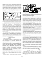
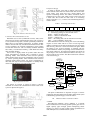
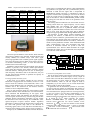
Fig. 9. Linear Decorrelator Strategy (LDS) in SDMA
IV.
EXPERIMENTS AND SIMULATIONS
To compare the proposed solution, we have made two kinds
of experiments to test the performance of DataTruck.
In the real experiments, we use DataTruck (with single
antenna) to gather data from static sensor nodes. There are 20
static nodes in the room, and DataTruck knows the position of
each node, it visits all nodes along a fixed trajectory and each
node is visited once in every round.
The DataTruck is equipped with an infrared ranging module
which is used to avoid the barrier. When DataTruck find the
barrier it will turn left or right with an angle of 30 degree,
then it will go to the position along prior direction using the
electronic compass module.
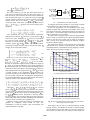
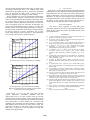
We compare the lifetime of network and the average data
transmission delay between using DataTruck and multihop
transmitting directly with different sensing frequency of static
nodes. The results are shown in Figure 10.
500
(4)
using DataTruck
no mobile sink
450
From Eq. (3), we can see that the signal part of
are
and
, respectively.
Lifetime of network(Minutes)
400
and
Since
and
, we can further
see that the projection operation always reduces the length of
unless
is already orthogonal to the spatial signature of
the other data stream. This is the overhead for nulling out the
would be in
interference. Hence, the effective channel for
deep fading whenever the projection of
onto
is small.
A similar situation is also applicable to
. Therefore, for
given transmission power of each sensor, not any two sensors
can successfully transmit data to DataTruck simultaneously.
To ensure the DataTruck can successfully decode the received
signal, the follow criteria should be satisfied
350
300
250
200
150
100
50
0
0
10
20
30
40
50
60
Number of sensing in 5 minutes
70
80
(a) sensing frequency VS. lifetime of network
80
using DataTruck
no mobile sink
70
60
where
,
,
and
are received
power and
of the received data from the two sensors,
respectively,
is denoted as the transmission power of each
sensor, and
is the receive sensitivity threshold while
is
the
threshold for the DataTruck to correctly decode
the received data. Any two sensors that satisfy this criteria can
successfully make concurrent data uploading to the DataTruck.
Such two sensors are said to be compatible [12].
Therefore, when we select the trajectory of DataTruck, the
position of compatible nodes should be took into
consideration to find the shortest path of DataTruck and
collect maximum size of data.
Average data delay(s)
(5)
50
40
30
20
10
0
0
10
20
30
40
50
60
Number of sensing in 5 minutes
70
80
(b) sensing frequency VS. average transmission delay
Fig. 10. The relationship between sensing frequency and lifetime
and average transmission delay
From Figure 10(a) we can see, while the frequency of data
sensing increases, the lifetime of network is reduced rapidly
with no mobile sink, because there are “hot spot” problem in
this network, the nodes near base station will die quickly for
2093