Download njit-etd1999-095

Copyright Warning & Restrictions
The copyright law of the United States (Title 17, United
States Code) governs the making of photocopies or other
reproductions of copyrighted material.
Under certain conditions specified in the law, libraries and
archives are authorized to furnish a photocopy or other
reproduction. One of these specified conditions is that the
photocopy or reproduction is not to be “used for any
purpose other than private study, scholarship, or research.”
If a, user makes a request for, or later uses, a photocopy or
reproduction for purposes in excess of “fair use” that user
may be liable for copyright infringement,
This institution reserves the right to refuse to accept a
copying order if, in its judgment, fulfillment of the order
would involve violation of copyright law.
Please Note: The author retains the copyright while the
New Jersey Institute of Technology reserves the right to
distribute this thesis or dissertation
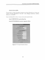
Printing note: If you do not wish to print this page, then select
“Pages from: first page # to: last page #” on the print dialog screen
The Van Houten library has removed some of the
personal information and all signatures from the
approval page and biographical sketches of theses
and dissertations in order to protect the identity of
NJIT graduates and faculty.
ABSTRACT
DEVELOPMENT OF A COMPUTER MODEL AND EXPERT SYSTEM
FOR PNEUMATIC FRACTURING OF GEOLOGIC FORMATIONS
by
Brian Michael Sielski
The objective of this study was the development of a new computer program called
PF-Model to analyze pneumatic fracturing of geologic formations. Pneumatic fracturing
is an in situ remediation process that involves injecting high pressure gas into soil or rock
matrices to enhance permeability, as well as to introduce liquid and solid amendments.
PF-Model has two principal components: (1) Site Screening, which heuristically
evaluates sites with regard to process applicability; and (2) System Design, which uses
the numerical solution of a coupled algorithm to generate preliminary design parameters.
Designed as an expert system, the Site Screening component is a high
performance computer program capable of simulating human expertise within a narrow
domain. The reasoning process is controlled by the inference engine, which uses
subjective probability theory (based on Bayes' theorem) to handle uncertainty. The
expert system also contains an extensive knowledge base of geotechnical data related to
field performance of pneumatic fracturing. The hierarchical order of importance
established for the geotechnical properties was formation type, depth, consistency/relative
density, plasticity, fracture frequency, weathering, and depth of water table.
The expert system was validated by a panel of five experts who rated selected
sites on the applicability of the three main variants of pneumatic fracturing. Overall,
PF-Model demonstrated better than an 80% agreement with the expert panel.
The System Design component was programmed with structured algorithms to
accomplish two main functions: (1) to estimate fracture aperture and radius (Fracture
Prediction Mode); and (2) to calibrate post-fracture Young's modulus and pneumatic
conductivity (Calibration Mode). The Fracture Prediction Mode uses numerical analysis
to converge on a solution by considering the three coupled physical processes that affect
fracture propagation: pressure distribution, leakoff, and deflection. The Calibration Mode
regresses modulus using a modified deflection equation, and then converges on the
conductivity in a method similar to the Fracture Prediction Mode.
The System Design component was validated and calibrated for each of the 14
different geologic formation types supported by the program. Validation was done by
comparing the results of PF-Model to the original mathematical model. For the
calibration process, default values for flow rate, density, Poisson's ratio, modulus, and
pneumatic conductivity were established by regression until the model simulated, in
general, actual site behavior.
PF-Model was programmed in Visual Basic 5.0 and features a menu driven GUI.
Three extensive default libraries are provided: probabilistic knowledge base, flownet
shape factors, and geotechnical defaults. Users can conveniently access and modify the
default libraries to reflect evolving trends and knowledge.
Recommendations for future study are included in the work.
DEVELOPMENT OF A COMPUTER MODEL AND EXPERT SYSTEM
FOR PNEUMATIC FRACTURING OF GEOLOGIC FORMATIONS
by
Brian Michael Sielski
A Dissertation
Submitted to the Faculty of
New Jersey Institute of Technology
in Partial Fulfillment of the Requirements for the Degree of
Doctor of Philosophy
Department of Civil and Environmental Engineering
May 1999
Copyright © 1999 by Brian Michael Sielski
ALL RIGHTS RESERVED
APPROVAL PAGE
DEVELOPMENT OF A COMPUTER MODEL AND EXPERT SYSTEM
FOR PNEUMATIC FRACTURING OF GEOLOGIC FORMATIONS
Brian Michael Sielski
Dr. John R. Schuring, Dissertation Advisor
Professor of Civil and Environmental Engineering, NJIT
Date
Dr. Paul C. Chan, Committee Member
Professor of Civil and Environmental Engineering, NJIT
Date
Edward G. Dauenheimer, Committee Member Professor of Civil and Environmental Engineering, NJIT
Date
Dr. Robert Dresnack, Committee Member
Professor of Civil and Environmental Engineering, NJIT
Date
Dr. John W. Ryon, Committee Member
Professor of Computer and Information Science, NJIT
Date
BIOGRAPHICAL SKETCH
Author:
Brian Michael Sielski
Degree:
Doctor of Philosophy
Date:
May 1999
Graduate and Undergraduate Education:
•
Doctor of Philosophy in Civil Engineering,
New Jersey Institute of Technology, Newark, NJ, 1999
•
Master of Science in Environmental Engineering,
New Jersey Institute of Technology, Newark, NJ, 1994
Bachelor of Science in Electrical Engineering,
The Pennsylvania State University, University Park, PA, 1988
Civil Engineering
Major:
Professional Background:
•
Research Assistant, Department of Civil Engineering, 1997 - 1999
New Jersey Institute of Technology. Newark, NJ
•
Teaching Assistant, Department of Civil Engineering, 1994 - 1997
New Jersey Institute of Technology. Newark, NJ
•
Electrical Engineer, 1988 - 1992
Kearfott Guidance & Navigation Corp. Wayne, NJ
Presentations and Publications:
Sielski, B., Schuring, J., Hall, H., Fernandez, H., and De Biasi, V. "Pneumatic Fracturing
Computer Model." H SRC/WERC Joint Conference on the Environment.
Albuquerque, NM, 21-23 May 1996.
iv
To My Loving Parents
ACKNOWLEDGEMENT
I owe a great debt of thanks to my dissertation advisor, Dr. John Schuring, for his
inspiration, encouragement, and guidance throughout this research. His vision,
friendship, and work ethic have guided me through this exciting journey, and his
unselfish kindness and compassion has set an example that will be with me for the
remaining days of my life.
I also wish to thank Professors Paul Chan, Edward Dauenheimer, Robert
Dresnack, and John Ryon for serving as members of the committee and for their careful
review and suggestions.
I am indebted to Tom Boland for his behind the scene efforts that enabled me to
complete this research in a timely manner. I would also like to thank him, as well as
Trevor King of McLaren/Hart Environmental Engineering Corp. and John Liskowitz,
President of ARS Technologies, Inc., for their expert opinion for the pneumatic fracturing
knowledge base.
I would like to thank the past students of the pneumatic fracturing project, many
of whom I do not know personally. Their work and research over the past decade has
aided greatly in understanding the technology. I'd like to especially thank Suresh
Puppala, as his research has been invaluable throughout this study.
Special appreciation is extended to Dr. Richard Scherl and Chris Koebel who are
responsible for wresting me from the security blanket of subjective probability theory
into the cold darkness of Bayesian networks and influence diagrams.
vi
I take great pleasure in recognizing my academic colleagues who have been
generous with their time and ideas: Michael "T-Time" Galbraith, Heather "Holistic"
Hall, Jenny "Quick Fingers" Lin, and Chip. Their friendship and goodness will always
be with me.
I am greatly indebted to my family and friends for reminding me why it all
matters, making me feel useful, sheltering me from the travails of the real world, and
surrounding me with so much love, support, and hope.
Finally, I'd like to thank all my maternal and paternal ancestors for providing me
with the correct DNA sequence to be here today.
vi i
TABLE OF CONTENTS
Page
Chapter
1 INTRODUCTION AND OBJECTIVES
1
1.1 Introduction
1
3
2 BACKGROUND INFORMATION 6
1.2 Objectives and Scope
6
2.1 Expert Systems 6
2.1.1 Introduction to Expert Systems 2.1.1.1 Origins of Expert Systems 7
2.1.1.2 Characteristics of Expert Systems 8
2.1.2 Expert Systems Architecture 11
2.1.3 Problem Solving Strategies Using Expert Systems 16
2.1.3.1 General Approaches
2.1.3.2 Control Strategies
2.1.3.3 Handling Uncertainty 2.2 Site Screening Model Background 16
17
19
24.
2.2.1 Geotechnical Properties 24
2.3 System Design Model Background 33
3 PROGRAM AND MODEL APPROACH 35
3.1 Overview of Concept and Model Components 35
37
3.1.1 Site Screening v iii
TABLE OF CONTENTS
(Continued)
Chapter
Page
3.1.2 System Design 38
3.1.2.1 Calibration Mode 39
3.1.2.2 Consistency and Strength of Clay Soils 39
41
3.1.3 Future Components 3.2 Site Screening Approach 42
3.3 System Design Approach 51
3.3.1 Physical Processes 51
3.3.2 Coupling the Physical Processes 55
3.3.3 System Design Algorithm 56
56
3.3.3.1 System Design Subroutine 3.3.3.2 Model Engine Subroutine
61
66
3.3.3.3 PDF Subroutine 73
3.4 Calibration Mode 3.4.1 Calibration Algorithm
73
74
3.4.1.1 Calibration Subroutine 3.5 Program Language and Structure
4 VALIDATION AND CALIBRATION OF PF-MODEL 4.1 Introduction
79
83
83
83
4.2 Site Screening 4.2.1 System Validation of Site Screening Component ix
84
TABLE OF CONTENTS
(Continued)
Chapter
Page
4.2.2 User Acceptance of Site Screening Component 4.3 System Design 88
94
4.3.1 Validation of the System Design Component 95
4.3.1.1 Validation of Calibration Mode 95
4.3.1.2 Validation of Fracture Prediction Mode 97
4.3.2 Calibration of the System Design Component 99
4.3.2.1 Calibration of Fine-Grained Soils 101
4.3.2.2 Calibration of Rock Formations 103
4.3.2.3 Calibration of Coarse-Grained Soils 105
107
5 RESULTS, CONCLUSIONS, AND RECOMMENDATIONS 5.1 Results and Conclusions 107
5.2 Recommendations 114
121
APPENDIX A SUBJECTIVE PROBABILITY THEORY APPENDIX B DEMPSTER-SHAFER THEORY
APPENDIX C BAYESIAN NETWORKS APPLIED TO PF-MODEL C.1 Background
126
128
128
C.2 Geologic Evidence 128
C.3 Approaches 129
C.4 Discussion 135
TABLE OF CONTENTS
(Continued)
Chapter
Page
APPENDIX D DEFAULT VALUES FOR GEOTECHNICAL PROPERTIES
IN PF-MODEL
138
APPENDIX E PROBABILITIES FOR PF-MODEL'S KNOWLEDGE BASE 142
APPENDIX F SUBJECTIVE PROBABILITY SITE SCREENING EXAMPLE 156
APPENDIX G SHAPE FACTORS USED BY PF-MODEL'S
GRAPHICAL ENGINE 160
APPENDIX F1 USER'S MANUAL FOR PF-MODEL 164
APPENDIX I SELECTIONS OF PROGRAM CODE USED IN PF-MODEL 189
I.1 Introduction
189
190
1.2 Selected Code for the System Design Routine 1.3 Selected Code from the Site Screening Component
1.4 Selected Code for the Data Input Screen
199
905
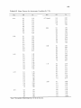
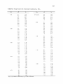
APPENDIX J TABLES USED IN VALIDATION AND CALIBRATION
OF PF-MODEL
711
REFERENCES
717
xi
LIST OF TABLES
Table
Page
2.1 Differences Between Conventional Programs and Expert Systems 2.2 Particle Size Classifications 7
25
2.3 Description of Atterberg Limit Range 28
2.4 Standard Penetration Test 30
2.5 Standard Scale for Fracture Frequency for Field Classification of Rocks 32
3.1 Guide to Consistency and Strength of Clay Soils 40
3.2 Approximate Relationship Between Consistency, Consolidation, and OCR 41
3.3 Assigned Permeability Enhancement Probabilities for the Site Screening
Component of PF-Model 45
3.4 Geologic Properties that Apply to Fine-Grained Soils 46
3.5 Geologic Properties that Apply to Coarse-Grained Soils 47
3.6 Geologic Properties that Apply to Rocks 47
3.7 Input Parameters for the System Design Subroutine
58
3.8 Deflection Solvers and Corresponding Equations 60
3.9 Rules, Interval Determination, and Actions for the Bisection Engine 64
3.10 The Coefficient, A. , for Soil and Rock Formations Varying with
Injection Flow Rate
69
3.11 Rules, Interval Determination, and Actions for the Calibration Mode 78
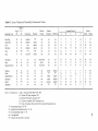
4.1 System Validation of Permeability Enhancement Variant .87
4.2 Hierarchical Order of Geotechnical Properties 92
xi i
LIST OF TABLES
(Continued)
Page
Table
4.3 Breakdown of Geotechnical Properties Into Qualifiers 93
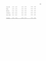
4.4 Validation of Calibration Mode for Estimating Young's Modulus 96
4.5 Validation of Calibration Mode for Estimating Pneumatic Conductivity
98
4.6 Validation of Graphical Leakoff Method (K h = 5Kv ) Using Bisection
Model Engine
100
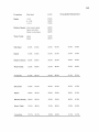
4.7 Calibration of Default Values for Fine-Grained Soils 102
4.8 Calibration of Default Values for Rocks 104
4.9 Calibration of Default Values for Coarse-Grained Soils 106
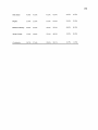
D.1 Default Values for Plastic, Fine-Grained Soils Used in PF-Model v3.0 139
D.2 Default Values for Coarse-Grained Soils Used in PF-Model v3.0
140
D.3 Default Values for Rocks Used in PF-Model v3.0 141
E.1 PF-Model's Knowledge Base Probabilities for Three Pneumatic
Fracturing Variants
143
G.1 Shape Factors for Isotropic Condition K h K,, 161
G.2 Shape Factors for Anisotropic Condition K 1 , = 5K,
162
G.3 Shape Factors for Anisotropic Condition K h = 10K,
163
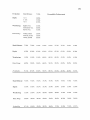
J.1 System Validation of Dry Media Injection Variant 212
J.2 System Validation of Liquid Media Injection Variant 213
J.3 Validation of Graphical Leakoff Method (K 1 , = K,,) Using Bisection
Model Engine "714
LIST OF TABLES
(Continued)
Page
Table
J.4 Validation of Graphical Leakoff Method (K h = 10KV ) Using Bisection
Model Engine
215
J.5 Validation of Analytical Leakoff Method Using Bisection Model Engine 216
xiv
LIST OF FIGURES
Figure
Page
2.1 Relationship of Expert System Components 12
22 Pneumatic Fracturing Process 3.1 Conceptualization of the Technology Transfer Process 36
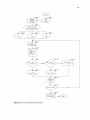
3.2 Top Level Flow Chart Showing the Model Components 37
3.3 Flow Chart of Site Screening Component 43
3.4 Flow Chart Representing How Inference Engine Accesses Probabilities
from Knowledge Base 48
3.5 The System Design Subroutine
57
3.6 The Model Engine Subroutine 62
3.7 The PDF Subroutine 67
3.8 The Calibration Subroutine 75
3.9 Interaction of Components, Engines, and Data Bases 82
C.1 Converging Connection 130
C.2 Earliest Version of a Bayesian Network Applied to Pneumatic Fracturing 131
C.3 A Bayesian Network for Plastic, Fine-Grained Soils 132
C.4 Bayesian Network for Rocks 133
C.5 Bayesian Network for Non-Plastic Soils 133
C.6 Bayesian Network of Plastic, Fine-Grained Soils with Example of
Divorced Parents 134
C.7 Bayesian Network Modeling the Success of Pneumatic Fracturing for
Plastic, Fine-Grained Soils
135
XV
LIST OF SYMBOLS
xvi
LIST OF SYMBOLS
(Continued)
xvii
LIST OF SYMBOLS
(Continued)
xviii
LIST OF SYMBOLS
(Continued)
LIST OF SYMBOLS
(Continued)
XX
CHAPTER 1
INTRODUCTION AND OBJECTIVES
1.1 Introduction
Over the past 25 years, industry, government, and the general public have become
increasingly aware of the need to respond to the hazardous waste problem, which has
grown steadily over the past 50 years. In 1980, Congress enacted the Comprehensive
Environmental Response, Compensation, and Liability Act (CERCLA) - the Superfund
Law - to provide for "liability, compensation, cleanup, and emergency response for
hazardous substances released into the environment and the cleanup of inactive waste
disposal sites."
A major difficulty in cleaning up some hazardous waste sites is the relative low
permeability of the formation (i.e., fine-grained soils and dense bedrock). Current
remediation technologies such as pump and treat, air sparging, bioremediation, vapor
extraction, thermal treatment, and soil washing work best in formations of relatively high
permeability. In response to this problem of low permeability formations, a research
effort was begun in 1987 at the Hazardous Substance Management Research Center
(HSMRC) at New Jersey Institute of Technology (MIT). It culminated with the
development of a new remediation enhancement technology known as "pneumatic
fracturing" (U.S. Patent # 5,032,042) in 1991.
Pneumatic fracturing enhances the permeability of contaminated geologic
formations by injecting high pressure air creating fractures or fissures in the soil or rock
matrix. The fractures or fissures occur if the injection is performed at a pressure which
1
2
exceeds the natural in situ stresses, and at a flow rate which exceeds the permeability of
the formation. In soil formations, pneumatic fracturing enhances the permeability of the
formation by creating fracture networks, while in rock formations, the effect is the
dilation and extension of existing discontinuities which improves the interconnection
between existing fractures. The immediate benefit is improved access to the subsurface
contaminants so that liquids and vapors can be transported and extracted more rapidly.
Pneumatic fracturing is similar in concept to the hydraulic fracturing techniques
used in the petroleum industry (Gidley et al., 1989). The principal difference is that
hydraulic fracturing uses water to create the fractures, while pneumatic fracturing uses a
gas (usually air). This is a significant and advantageous difference. In using air as an
injection fluid, fracture propagation is more rapid due to the lower viscosity of air over
water. In addition, air is less likely to remobilize and spread contaminants than water.
Pneumatic fracturing has been successfully demonstrated in the field at a number
of contaminated sites. Among these are U.S. EPA SITE Demonstrations at contaminated
sites in Hillsborough, New Jersey, to enhance soil vapor extraction (U.S. EPA, 1993) and
in Marcus Hook, Pennsylvania, to enhance in situ bioremediation (U.S. EPA, 1995).
Pneumatic fracturing is now available commercially for enhancement of pump and treat,
vapor extraction, air sparging, and bioremediation. Other innovative approaches using
the pneumatic fracturing process are also under investigation, and include in situ
vitrification, in situ ultrasonic enhancement, and reactive media injection.
3
1.2 Objectives and Scope
The objective of this study is to develop a comprehensive pneumatic fracturing computer
model (called PF-Model) with two principal functions. First, the model will assist in
deciding whether or not a site is a potential candidate for the technology. Second, it will
generate preliminary design parameters for applying the pneumatic fracturing process at
the site. Each of these model functions will now be briefly introduced.
An essential step in the successful remediation of a site is the selection of
appropriate technologies. In the past, the decision when and if to use pneumatic
fracturing was made by informal quantitative comparisons with empirical data from past
projects by an expert familiar with the capabilities of the technology. Now, the computer
model will make the same judgment by functioning, in part, as an "expert system."
An expert system is a high performance problem-solving computer program
capable of simulating human expertise within a narrow domain. An expert system either
performs the function of a human being, or it fulfills the role as an assistant to the human
decision maker. Expert systems are best suited for conditions in which there are no
efficient algorithmic solutions (Biondo, 1990), such as the decision of whether a site is a
potential candidate for pneumatic fracturing.
Once PF-Model has determined that pneumatic fracturing is an appropriate
technology for the site, the program will then make preliminary estimations of design
parameters such as well spacing, injection pressures, and fracture intervals. This part of
the program incorporates current mathematical models developed at the Center for
Environmental Engineering and Science (CEES) (Puppala, 1998, and King, 1993). The
4
coding of this part of the computer model uses conventional programming techniques,
since mathematical models and algorithmic solutions require rigid control structures.
The computer model is designed in a WindowsTM format that is interactive with
the user. The program makes extensive use of graphics and objects, thus providing a
friendly user interface. The computer program also includes a User's Guide for design
applications.
A data base library of probabilities representing geologic evidence necessary for
site screening is also included in PF-Model. This part of the program allows the data
base to be updated with new probabilities as desired, allowing "expert" potential users to
customize their own proprietary version of the program. The library provides the expert
system with the needed information (i.e., probabilities) to assess pneumatic fracturing
applicability, dry media injections, and liquid media injections based on the geologic
evidence that is known and subsequently entered as data.
The final phase of the study involves validation of the predictive aspects of the
computer model, especially those parts coded as an expert system. Since 1989, a
considerable amount of field data has been collected and was available to calibrate the
propagation model. Likewise, for site screening, calibration is based on actual past field
demonstrations combined with heuristic reasoning. In addition, the model is run for
hypothetical sites to "push the envelope" of the pneumatic fracturing technology in
consultation with current experts in the field.
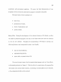
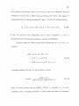
In summary, the objectives of this research study are to:
1. Investigate various probabilistic options available for an expert system.
5
2. Design and code an expert system to make technology
recommendations.
3. Convert available analytical and numerical component models to
computer code in order to make preliminary estimates of design
parameters used in the technology.
4. Establish an overall design and logic implementing a Windows TM
format program.
5. Include a User's Guide for design applications.
6. Develop an interactive knowledge base containing the probabilities for
pneumatic fracturing applications for previous and future site data and
technology information.
7. Develop a library of system and geotechnical defaults for PF-Model to
support the System Design component for estimating fracture radius
and aperture.
This dissertation will begin with a summary of expert systems, site screening, and
propagation model backgrounds (Chapter 2). This will be followed by a discussion of the
approach for the different model components and how they are coded and/or theorized
(Chapter 3). Next, the model will be field validated and calibrated with data from
previous sites and discussion with experts (Chapter 4). Finally, conclusions and
recommendations for future study are presented (Chapter 5). The User's Guide for
PF-Model is included in Appendix H.
CHAPTER 2
BACKGROUND INFORMATION
This chapter will provide the reader with appropriate background information used in
programming the computer model. First, since some components of the computer model
are in part based on expert systems, an introduction to expert systems is presented.
Second, the parameters, or geologic evidence, required for successful application of the
site screening model will be described. Finally, the analytical model used in solving
fracture propagation and associated research will be discussed.
2.1 Expert Systems
The overall objective of the study is to "capture" the available knowledge of the
pneumatic fracturing process, thus allowing distribution of this expertise on a wider scale.
PF-Model encompasses both a heuristic model (i.e., the Site Screening component) and
an analytical model (i.e., the System Design component). The Site Screening component
is based on the development of an expert system which generates technology
recommendations. This section provides an overview of current expert system
technology and theory, as well as the advantages and disadvantages.
2.1.1 Introduction to Expert Systems
Expert systems, or knowledge-based expert systems, are computer programs that
represent and use the knowledge of some human expert in order to solve problems or give
advice within a narrowly defined field or domain (Durkin, 1994). This definition does
6
7
not distinguish the difference between expert systems and conventional programs and
techniques, however. Conventional programs can be interactive and contain rules of
selection/decision, yet still not be an expert system. Table 2.1 shows the important
differences between expert systems and conventional programs.
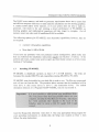
Table 2.1 Differences Between Conventional Programs and Expert Systems (Maher,
1987).
Conventional programs
Representation and use of data
Knowledge and control integrated
Algorithmic (repetitive) process
Effective manipulation of data bases
Oriented toward numerical processing
Expert systems
Representation and use of knowledge
Knowledge and control separated
Heuristic (inferential) process
Effective manipulation of knowledge bases
Orientated toward symbolic processing
2.1.1.1 Origins of Expert Systems: Early computers were originally high speed data
processors. Programs were written based on a prescribed algorithm to perform a series of
specific actions, or tasks. The programs solved equations, processed data, and scanned
data bases for information. They were able to do this exceptionally well, but they were
still not able to reason about the information they were processing. Any problem that
required human reasoning was performed by a human expert (Shapiro, 1987).
Eventually, programmers began coding knowledge about a problem into the
computer. The knowledge consisted of facts, rules, and structures of the problem which
was coded in "symbolic" form. The problem knowledge was represented as symbols,
which is simply alphanumeric characters. In order to encode and search through the
8
symbolic information, symbolic processing languages were developed. Some early
examples of symbolic languages include LISP and PROLOG (Michie, 1979).
As advances in symbolic programming languages and symbolic knowledge
representation were made in the late 1950s, programmers began efforts to create
programs that displayed intelligent behavior. This created a new field of study called
Artificial Intelligence, or Al (Shapiro, 1987).
Al strives to simulate human intelligence in a computer. Early Al research
centered around the belief that a few laws of reasoning paired with computers would be
able to simulate human intelligence. After years of research in developing Al programs,
it was found that the general problem-solving strategies were too weak to solve most
complex problems (Newell and Simon, 1972). This is because solution of a specific
problem required quality knowledge within some narrow domain to successfully search
for a solution. Eventually, the technology known as "expert systems" grew out of the Al
branch of computer science (Patterson, 1990). In essence, an expert system is an Al
program with specialized problem-solving expertise.
2.1.1.2 Characteristics of Expert Systems: The best way to introduce the concept of an
expert system is to describe characteristics which are common to all expert systems.
These are listed and briefly discussed below.
Limited to Solvable Problems. It may seem surprising, but before the development of an
expert system begins, it must be determined if the problem is solvable. An expert system
will not work if there is no human expert available to obtain knowledge from. New or
9
novel research issues are therefore not candidates for expert systems programming
(Prerau, 1985).
Possesses Expert Knowledge. An expert system must capture and encode the knowledge
of a human expert, including the expert's problem-solving skills and his domain
knowledge. These skills or knowledge are not necessarily unique or brilliant, rather they
are known only by a few others.
Focuses Expertise. Focusing the expertise should seem obvious, but in fact,
programmers who have designed expert systems to encompass broad topics have
achieved little success and failed (Ham, 1984, and Prerau, 1985). Expert systems do not
perform well when tasked with problems outside their area of expertise, just like humans.
An expert system can be successfully developed only when the scope of the problem is
well defined.
Reasons Symbolically. The knowledge used by an expert system can be expressed in
symbolic terms rather than numerical terms. Symbols can represent facts, concepts, and
rules. Problems are solved by manipulating symbols rather than by numeric processing
(i.e., conventional programs).
Reasons Heuristically. Heuristics is the study or practice of procedures that are valuable
but are incapable of proof (Lenat, 1982). A human expert possesses more than just public
knowledge, i.e., knowledge which is available in published literature. A human expert
10
uses not only facts and theories to solve a problem, but also considers past experiences.
Such knowledge gives the expert a practical understanding of the problem and allows the
development of "rules-of-thumb," or heuristics, to solve the problem.
To illustrate the difference between conventional programs that use algorithms
and expert systems that often use heuristic techniques, consider the example of a bicycle
chain which keeps coming off while riding, an indication of a stretched chain. The
conventional algorithm is a series of orders or calculations that are well structured:
1. Measure the length of chain.
2. Count the number of chain links.
3. Compute link to length ratio.
4. If ratio > 1.1, then chain is stretched.
The algorithm performs this same sequence of operations each and every time. It is this
repetitiveness that makes it attractive for conventional programming techniques.
Heuristic reasoning does not follow a rigid structure of steps (Georgeff, 1983).
Rather, it draws a conclusion based on the available information. The heuristic approach
to determine if the chain is stretched would be as follows:
IF
Chain comes off bike
AND
Chain is old
THEN
Suspect stretched chain.
11
Notice that heuristic reasoning does not guarantee that the chain is actually stretched, but
it is a good starting point to begin analysis of the problem. The problem may actually
have been a faulty rear derailleur or worn chainrings.
Makes Mistakes. It must be recognized that since expert systems are programmed with
the knowledge of a human expert, they are therefore capable of making the same
mistakes. That is not to say conventional programs with structured algorithms have a
significant advantage over expert systems. Both types of programs address different
types of problems. Conventional programs work well where information or data is
readily available or certain. But if the data is wrong or incomplete, a conventional
program will return a wrong result, or nothing at all. Expert systems are designed to
work with less information. The result may not be exact, but it can be reasonable.
Other Characteristics. Expert systems usually exhibit some other common
characteristics. First, expert systems must perform at a competence level which is equal
to or better than an expert in the field. It should also reach decisions within a reasonable
amount of time. Finally, the system should have a stable platform and not be subject to
crashing or freezing up.
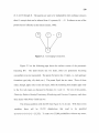
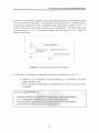
2.1.2 Expert Systems Architecture
There are three major traits of an expert that are modeled in an expert system: (1) the
expert's knowledge in the specific domain; (2) the reasoning used to reach a conclusion
or provide an answer; and (3) knowledge about the problem being solved. To accomplish
12
this, the expert system must be designed with a number of interactive working
components. They have three principal components: a knowledge base, the working
memory, and an inference engine. Other components that can enhance the model are a
user interface, explanation facility, and knowledge acquisition facility (Durkin, 1994).
Figure 2.1 shows an idealized representation of the architecture of an expert system and
the relationship between its components.
Inference
Engine
Knowledge
Acquisition
Facility
Knowledge
Base
Figure 2.1 Relationship of Expert System Components.
The remainder of this section will discuss each of these components, all of which are
needed to build an expert system.
13
Knowledge Base. The knowledge base is the part of the expert system that contains the
domain knowledge and heuristics of the expert. In general, it is the collection of
knowledge in the form of rules, procedures, and facts. The most typical way to represent
the heuristics of the expert is to apply an IF/THEN decision structure (Georgeff, 1983).
The knowledge base also contains a high level of competence in the general knowledge
about the behavior and interactions in the problem domain. The scheme of the
knowledge base is one of the most critical decisions in that it impacts the design of the
inference engine, the knowledge acquisition facility, and overall efficiency of the system
(Stefik el al., 1982).
Working Memory. The working memory is the component of the expert system that
models the human's short term memory. It contains the global data base used by the
rules of the system, facts both entered and inferred, and the intermediate results that make
up the current state of the problem (Hunt, 1986). Eventually, the working memory
expands as the expert system reasons about the current problem. Information and data
subsequently generated by the expert system in order to solve the problem are also stored.
When the problem is solved, the working memory not only contains the solution, but all
the intermediate results as well.
Inference Engine. Also known as the control structure or rule interpreter, the inference
engine is the part of the program that performs the reasoning. It locates the required
knowledge and infers new knowledge from the base knowledge. Armed with the control
information, it uses the knowledge base to match facts in the working memory. When the
14
inference engine finds a match, it will add the -tile's condition to the working memory
and continue to scan for other possible matches. The inference engine must also have the
capability to modify and expand the knowledge base to draw conclusions about the
problem.
The search strategy used by the inference engine to develop the required
knowledge, or inference paradigm, can be one of three fundamental types (Bielawski and
Lewand, 1988): (1) forward chaining, which starts with known conditions and works
toward a desired goal; (2) backward chaining, which starts from the desired goal and
works backward toward supporting conditions; or ( 3 ) mixed chaining, which is a
combination of both forward and backward chaining. These search strategies for the
inference engine will be further discussed in Section 2.1.3, "Problem Solving Strategies
Using Expert Systems."
Since the inference engine is detached from the knowledge base, changes can be
made to either component without necessarily having to alter the other. For example, one
may be able to add information to the knowledge base, or increase the performance of the
inference engine, without having to modify code elsewhere (Clancey, 1983). That is not
to say that the inference engine is totally independent of the knowledge base. On the
contrary, they are intimately related. Should the inference engine control the reasoning
process at a very low level (i.e., providing solution strategy flexibility), the knowledge
base must contain concise and specific data. On the other hand, if the inference engine
has a high-level reasoning process, the knowledge base does not need to be extensive.
The interaction between the knowledge base and inference engine constitutes the
major source of uncertainty in the expert system due to unreliable information,
15
incomplete information, or a poor combination of knowledge from different experts.
Therefore, the expert system must be capable of handling this uncertainty. Three popular
methods are subjective probability theory, the Dempster-Shafer theory, and more recently
Bayesian networks, all of which will be described later in Section 2.1.3, "Problem
Solving Strategies Using Expert Systems."
User Interface. This is how the user and the expert system communicate. The user
interface should interact in a natural language style and should be as close as possible to
humans in conversation in order to gather as much information as is possible. It may also
be designed to allow the interface to change information in the working memory should
this be desirable for the user.
The actual interface design can take on many variations. Today, most interfaces
are interactive and make extensive use of menus, graphics, and specifically designed
screens. Overall, the interface design should be as accommodating as possible.
Explanation Facility. An expert system should not just reach a conclusion when faced
with a complex problem, but be capable of explaining to some extent, some of the
reasoning that led to that conclusion. Since an expert system works on a problem that
lacks a rigid control structure, this capability takes on some importance in an expert
system due to the fact that the validity of the system's findings may come into question.
Why a particular question is asked allows the user to feel more comfortable with the line
of questioning, and understand what line of reasoning the system is pursuing.
16
Knowledge Acquisition Facility. In expert systems knowledge and data are constantly
changing and expanding, and the knowledge base must be modified accordingly. The
knowledge acquisition facility is an automatic way for the user to enter knowledge in the
system rather than by having the knowledge engineer explicitly code the knowledge
(Giarratano and Riley, 1989). The knowledge acquisition facility acts as an editor,
allowing new knowledge to be entered, or modifying existing knowledge.
2.1.3 Problem Solving Strategies Using Expert Systems
The search to solve a problem with an expert system begins with known facts or data, and
ends at a final conclusion or solution. This section discusses the various problem-solving
strategies including general approaches, control strategies, and handling uncertainty.
2.1.3.1 General Approaches: In expert systems there are two main approaches to solve
problems: the derivation approach and the formation approach (Maher, 1987). The
derivation approach starts at a known state and uses deductive logic to arrive at a known
solution. This approach is desirable if there are predefined solutions available in the
knowledge base of the expert system. This means that the expert system will provide a
solution based on the specifications of the given problem. If an inference network
between the predefined solutions and the input data can be achieved, the derivation
approach can be implemented.
The other general approach is the formation approach which uses information.
about the known state to generate more information to form higher level solutions.
Information from the knowledge base is used in order to form a solution. This method is
17
used when it is either impractical or impossible to store all the predefined solutions in the
knowledge base. The formation approach is implemented by identifying parts of the
solution and then heuristics to combine them.
2.1.3.2 Control Strategies: Many strategies for solving problems guided by the
knowledge contained in the knowledge base exist. The three most common control
strategies for choosing the next action, given many alternative problem-solving steps, are
presented next.
Forward Chaining. An expert system uses a forward chaining strategy if it works from
known facts to a conclusion. Forward chaining is advantageous since most problems
begin with the gathering of information and then seeing what conclusions or goals can be
reached from it. It can also provide information from only a small amount of input data.
Forward chaining operates by collecting all the initial information into the
working memory. The information can be obtained from either the data base or inputted
from the user. The system then scans the rules searching for a match. When a rule match
is found, it is executed, or fired, placing its conclusion in the working memory. The
scanning process is repeated again until no additional rules are fired.
It is possible that during a scan of the rules, several rules may be applicable.
Usually though, only one of these rules needs to be fired before the system cycles through
the rules again. This is called a recognize-resolve-act cycle (Durkin, 1994). There is also
the process called conflict resolution in which several rules compete, but only one is to be
18
fired. In this method, the rules are given a priority value in which the rule with the
highest priority fires.
Some disadvantages exist with a forward chaining system, however. There may
be no means for the system to recognize that some data might be more important than
others. The system will also ask all possible questions, or require all possible input data
for all possible conditions, which may not be known or relevant. Only a few questions
may have been needed to arrive at a conclusion.
Backward Chaining. Backward chaining involves reasoning from a conclusion or
hypothesis, backing through the rules in search of the facts which support or discount that
hypothesis. This type of control strategy can be advantageous since some problems begin
naturally by forming a hypothesis and then seeing if it can be proven: "I believe the chain
just fell off my bike." This strategy also focuses on the given goal, asking questions that
relate only to its solution. It searches the knowledge base that is relevant only to the
current problem, as opposed to forward chaining which attempts to infer everything
possible from all available information. The primary disadvantage of backward chaining
is that it will follow a given line of reasoning even if the goal is dropped and switches to a
different one (Durkin, 1994).
Backward chaining operates by collecting the set of rules that contain the solution
in the THEN part. These rules are called goal rules: rules that can be proven if one of
these goal rules fires. The goal rule will only fire if its premises are satisfied. These
premises are in turn supported by other rules, which requires the inference engine to
prove them as well. These are termed subgoals. The system then searches its rules
19
recursively to validate both the subgoals and the original goal. Eventually a premise is
reached that is not supported by any of the system's rules, i.e., a primitive. The system
may then ask the user other questions which will cause possible firing of other rules.
These conclusions are then added to the working memory.
The entire process repeats until all subgoals and goals have been searched. The
information provided by the user and inferred by the system are stored in working
memory. With an understanding of the original goal, this information determines if it is
true or false.
Mixed Chaining. The mixed chaining control strategy is when the system uses both
forward chaining and backward chaining strategies. The advantage of mixed chaining is
that the user supplies only the relevant information needed to solve the problem. If the
initial hypothesis is wrong, the system moves to the next assumption based on the current
information.
This strategy operates with known facts and assigns a probability to the potential
solutions or conclusions. It then attempts to support the highest priority solution by
creating subgoals and requesting additional information from the user if necessary. If the
conclusion is false, the system takes the next highest priority solution and then attempts
again to determine if the solution is true or false. This process is repeated until the
solution is true.
2.1.3.3 Handling Uncertainty: An expert system is required to reason with uncertain
information, so selecting an uncertainty theory to model the expert system becomes
20
important. A discussion of the more popular theories for handling uncertainty is
presented in the following.
Subjective Probability Theory. Subjective (or Bayesian) probability is used by most
expert systems since it is favored by system developers (Levitt, 1988 and Tzvieli, 1992).
This is because a knowledge base stores human knowledge and facts, and when
representing an expert's knowledge, it is usually viewed as subjective by the programmer.
Subjective probability is developed from the theory of partial belief, called
Bayesian theory after the English clergyman Thomas Bayes (1702-1761). The basic
premise is that all degrees of belief should obey certain rules. By attributing A as the
degree of belief p, given evidence B, the famous formula of Bayes can be stated (Pearl,
1988):
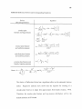
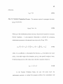
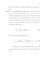
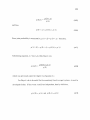
For Bayes' rule to handle the uncertainty found in expert systems, it must be developed
into a different form. The mathematical extension of Bayes' theorem, which is detailed
in Appendix A, yields the following basic equation for applying probability theory to
expert systems,
21
This states that the conditional probability of A given B can be obtained from the
conditional probability of B given A. For example, consider an expert system where the
rules are in the form: "If <A is true> Then <B will be observed with probability p>."
Clearly, if A is observed, then the probability of event B is p. But Equation 2-2 is also
applicable in the case when A is unknown and B is observed. Equation 2-2 can then be
used to compute the probability that A is true as well.
Dempster-Shafer Theory. The Dempster-Shafer theory was originally developed in the
1960s by Arthur Dempster (Dempster, 1967) and later extended by Glen Shafer (Shafer,
1976) in the 1970s. The development of the theory was driven by the two difficulties
Dempster and Shafer had with subjective probability theory. These were the
representation of ignorance, and the idea that the subjective beliefs assigned to an event
and its negation must sum to one (Ng and Abramson, 1990).
In probability theory, ignorance is represented by indifference or by uniform
probabilities. The problem believed here is that uniform probabilities seem to represent
more information than is known. Therefore, you can attribute equal prior beliefs to either
complete ignorance or equal belief in all hypotheses (or events). Also, when new data or
information does become available, the original ignorance expressed in the prior belief
may no longer be valid.
The mathematical development of the Dempster-Shafer theory is outlined in
Appendix B. Shafer believed that evidence which partially favors a hypothesis should
not be construed as also supporting its negation. This contrasts with subjective
22
probability theory, which states that once the probability of the occurrence is known, the
Bayesian Networks. One of the more promising belief networks that plays a central role
in handling uncertainty are Bayesian networks (Pearl, 1988). Bayesian networks handle
this uncertainty using probability theory and the formal use of diagrams. The diagrams
show important conceptual information about the network.
Bayesian networks are represented by directed acyclic graphs (a directed graph is
represents an uncertainty. The use of arrows in the directed graphs allow for
distinguishing dependencies between nodes by inspection. The probabilities assigned in
the network are conditional and quantify conceptual relationships in one's own mind, i.e.,
cause and effect. These are psychologically meaningful and can be obtained by direct
measurement or data analysis. Appendix C details Bayesian networks and discusses its
possible use as a model for the Site Screening component of PF-Model.
The greatest advantage of using directed graphs, such as Bayesian networks, is
that it is easier to quantify the directed links with local nodes, turning the network into a
globally consistent knowledge base (Pearl, 1988). The disadvantage of using a Bayesian
network when applied to the Site Screening component, as detailed in Appendix C, is the
subsequent scaling of posterior probabilities and assignment of priori probabilities to
geologic evidence.
23
Other Theories. Two other theories for dealing with uncertainty in expert systems are
possibility theory and the certainty factor approach. Possibility theory was developed by
Zadeh (1978) due to the difficulties he had with using probability theory's representation
of inexact or vague information. It is based on his theory of fuzzy sets. Possibility theory
expresses vague terms such as "very likely" or "probably" with precision and accuracy.
If these terms were coded with probability, their imprecision or "fuzziness" would be
lost, i.e., either the event occurred or it did not.
The advantage of possibility theory then is that events may be represented with
shades of gray since human knowledge of facts is very rarely precise. There are
disadvantages with fuzziness, however, that are identified in Cheeseman (1986), Stallings
(1977), Wise and Henrion (1986), and Giles (1982). The disadvantages include the
difficulty of interpreting fuzzy quantifiers and the necessity of fuzzy theories altogether.
In the 1970s, Shortliffe developed the certainty factor approach which he used in
the later development of MYCIN, a medical expert system for the diagnosis of infectious
blood diseases (Shortliffe and Buchanan, 1984). Shortliffe felt that probability theory
would not be appropriate (Shortliffe et al., 1979) for medical diagnosis, since decisions
can vary over a wide spectrum, from categorical reasoning on one extreme to
probabilistic at the other (Szolovits and Pauker, 1978). The certainty factor approach is
-
designed to handle these difficulties. Obviously, there were disadvantages with this
method, the most obvious brought out by Adams. He found, for example, that some
unstated assumptions made by certainty factors may not be valid (Adams, 1976).
24
2.2 Site Screening Model Background
An essential step in successful site remediation is selection of appropriate technologies.
Geotechnical properties play a major role in the decision process for in situ technologies
like pneumatic fracturing. This section discusses the various geotechnical properties
which are considered in the Site Screening component of PF-Model.
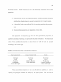
2.2.1 Geotechnical Properties
Years of experience and research with the pneumatic fracturing process have
demonstrated that the success of the technology (or its failure) is dependent on a number
of different geotechnical properties. This has led to a hierarchical ranking of the
geological properties. After careful consideration and discussion with experts, it has been
determined that seven different factors can significantly affect the pneumatic fracturing
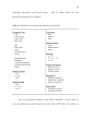
process (Sielski, 1998). They are presented below in the order of perceived importance.
•
Formation type
•
Depth
•
Plasticity (soils)
•
Relative Density/Consistency (soils)
•
Fracture frequency (rocks)
•
Weathering (rocks)
•
Water table
25
Each of these will now be discussed in the context of their importance to pneumatic
fracturing.
Formation Type.
For soils, texture is the most fundamental descriptor of the
geomaterial. The sizes of particles that make up soil vary over a wide range from clay
size (< 0.075 mm) all the way up to boulders (> 9 in.) (Burmister, 1970). A number of
different classification systems have been developed to describe particle size within an
engineering context. Table 2.2 shows the more common classification systems including
those developed by the U.S. Department of Agriculture (USDA), the American
Association of State Highway and Transportation Officials (AASHTO), and the Unified
Soil Classification System, (USCS) developed by the U.S. Army Corps of Engineers. In
the United States, the USCS is the most used.
Table 2.2 Particle Size Classifications (Das, 1994).
The principal effect of soil texture on pneumatic fracturing is that it largely
controls the permeability and porosity of the soil. This is related to the basic principle
26
that a pneumatic fracture will continue to propagate only as long the fluid injection rate
exceeds the ability of the soil pores to accept the fluid, i.e., the permeability. For
example, when air is injected into clay soils, the natural permeability of the formation can
not accept the air quick enough, and discrete fractures are created in the formation.
Conversely, in a coarse soil formation such as sand which has a relatively high
permeability, the effect of pneumatic fracturing is very different. Although there may be
some local fracturing around the borehole, for the most part the sand is able to accept the
injected air. In this instance, the main effect is rapid aeration as air passes through
interstitial pore spaces.
In cases where soils have a marginal permeability, it becomes difficult to predict
the effect pneumatic fracturing will have. In this instance, more evidence about the soil
formation is required.
In rocks, the lithology acts as the fundamental descriptor (type, color, mineral
composition, and grain size are all lithologic characteristics) (Boggs, 1987). The
principal effect of rock lithology on pneumatic fracturing is that it largely controls
discontinuities and interconnectivity.
For example, consider a sedimentary rock such as shale or sandstone.
Sedimentary rocks are formed by particle deposition and are characterized by their
distinctive layers. This layering, also known as stratification, imparts numerous and
regular discontinuities which dilate during pneumatic fracturing. A certain amount of
dilation is permanent, leading to substantial increases in permeability and
interconnectivity.
27
On the other hand, igneous and metamorphic rocks are not formed by particle
deposition and their existing discontinuities are mostly formed by thermal strain during
cooling or tectonic movements. Discontinuity patterns are less regular, and it is likely
that permeability and interconnectivity are more difficult to enhance. It is noted that,
unlike sedimentary rocks, experience with pneumatic fracturing of igneous and
metamorphic rocks is very limited.
Overall, when pneumatic fracturing is applied to a formation, there are expected
trends and predictable behaviors. Fine-grained soils and sedimentary rocks respond well
to permeability enhancement by pneumatic fracturing. In contrast, coarse-grained soils
(e.g., sand) already have substantial permeability and pneumatic fracturing is not.
appropriate for permeability enhancement. However, media injection by the pneumatic
fracturing process might still be recommended as an alternative technology variant for
coarse-grained soils. In summary, then, it is texture and lithology that largely determine
whether or not fractures will be formed, and also how fluids will move through the
formation. Thus, these are clearly the most important parameters in determining the
applicability of pneumatic fracturing, and they will be the dominant pieces of evidence in
the probabilistic model.
Depth. The depth of a formation is the second most important parameter in determining
whether or not pneumatic fracturing will be successful. Pneumatic fracturing projects to
date have reached depths of 50 ft, but there is no theoretical maximum depth limit. As
long as sufficient back pressure and flow can be delivered into the formation with higher
capacity equipment, fracturing can be propagated at greater depths.
28
The minimum depth of injection is based on the ability of the formation to act as a
"seal" during injection. For example, formations which are made of fill materials will
tend to exhibit "daylighting" which means that the fractures will intersect the ground
surface. However, formations such as rock will allow injections closer to the surface, i.e.,
3 ft, with minimal amounts of daylighting.
Plasticity. Another important property is plasticity. A soil that can be remolded in the
presence of some moisture without crumbling is said to be plastic. Plasticity applies only
to fine-grained soils when clay minerals are present (i.e., clay, clayey silt, clayey sand,
and silty clay). Soil plasticity is measured using the Atterberg Limits Test (ASTM
D4318-93) which correlates soil moisture content with plastic behavior. Descriptions of
soil consistency in relationship to Atterberg Limits are presented in Table 2.3.
Table 2.3 Description of Atterberg Limit Range.
It has generally been found that brittle soils (14) < PL) respond well to pneumatic
fracturing (Pisciotta et al., 1991, and Schuring ci al., 1991). Experience has shown that
soils which are in the plastic range (PL < w < LL) can also be successfully fractured.
29
However, post-fracture air flows in plastic soils may be retarded by moisture in the pores
and fractures.
As the moisture content of a clay soil increases above the liquid limit (1-1 > LL),
,
the soil exhibits a tendency to flow. Although there has been little field experience with
fracturing soils above the liquid limit, laboratory studies have shown that fracture healing
could be a problem (Hall, 1995).
Relative Density/Consistency. This geotechnical property is only used to describe soil
formations. Relative density is applied to cohesionless soils, e.g., sand, while consistency
is applied to cohesive soils, e.g., clay. The relative density/consistency is usually
obtained by the widely used standard penetration test or SPT (ASTM D1586-84), which
consists of driving a split spoon sampler into the ground by dropping a 140 lb. weight
from a height of 30 in. The sum of the blows required to drive the spoon is recorded and
is used to compute the standard penetration resistance, or N-value (Sowers and Sowers,
1970).
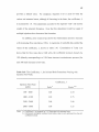
Table 2.4 on the following page shows a correlation between penetration
resistance and relative density for cohesionless soils, and a correlation between
penetration resistance and consistency for cohesive soils.
Relative density/consistency has two important influences on the propagation of
pneumatically induced fractures. First, it is an indication of the elastic modulus or
stiffness of soil formations. Loose or soft soil formations will usually exhibit localized
deformation around the injection point resulting in modest propagation radii. In contrast,
firm or stiff formations will deform less but influence radii will be larger.
30
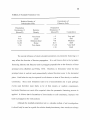
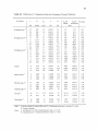
Table 2.4 Standard Penetration Test.
Consistency of
Cohesive Soils
Relative Density of
Cohesionless Soils
Penetration
Resistance, N
(blows/ft)
Relative
Density
0-4
4-10
10-30
30-50
> 50
Very loose
Loose
Medium dense
Dense
Very dense
Penetration
Resistance, N
(blows/ft)
Consistency
<2
2-4
4-8
8-15
15-30
> 30
Very soft
Soft
Medium
Stiff
Very Stiff
Hard
The second influence of relative density/consistency on pneumatic fracturing is it
may affect the direction of fracture propagation. It is well known that in the hydraulic
fracturing industry that fractures tend to propagate perpendicular to the direction of least
principal stress (Hubbert and Willis, 1957). Therefore, in formations where the least
principal stress is vertical, most pneumatically induced fractures occur in the horizontal
plane. Such behavior may be expected in soils that are at least of firm density or medium
consistency. Since most formations tend to be overconsolidated due to past geologic
events (and therefore more likely to be of firm density or medium consistency),
horizontal fractures are most often expected when the pneumatic fracturing process is
applied. It follows that in formations of loose density or soft consistency, fractures will
tend to propagate in the vertical plane.
Although the standard penetration test is a valuable method of soil investigation,
it should only be used as a guide for relative density/consistency since results are always
31
approximate (Lambe and Whitman, 1969). Therefore, caution must be applied when
applying this piece of evidence in the probabilistic model. In general, the standard
penetration test is considered more reliable for cohesionless soils than cohesive soils.
Fracture Frequency. Discontinuities, or fractures, occur naturally in rock formations,
originating from thermal and tectonic stresses, as well as unloading of overburden
materials. Various types of discontinuities are encountered including cracks, joints,
faults, and shear zones (Bates and Jackson, 1984). In general, rock formations of the
same lithology develop a somewhat similar discontinuity geometry. For example, basalt
commonly exhibits vertical columnar joints, while shale exhibits bedding joints.
Research over the last 10 years has shown that the principal effect that pneumatic
fracturing has on rock formations is that it dilates existing discontinuities. Thus, rocks
with fairly frequent fractures will respond best. Conversely, formations with only a few
widely spaced fractures are not good candidates for the pneumatic fracturing technology
since process pressures are not sufficient to break intact rock. It is further noted that
pneumatic fracturing may also have reduced effectiveness in intensely fractured rock
formations due to high leakoff rates. The standard scale for fracture frequency for field
classification of rocks is given in Table 2.5 on the following page.
Weathering. The breakdown of rocks by weathering involves three processes: chemical,
physical, and biological. The most important of these as it applies to pneumatic
fracturing is by far the chemical process. In the chemical process secondary minerals are
32
Table 2.5 Standard Scale for Fracture Frequency for Field Classification of Rocks.
Fracture Frequency
Spacing
Description for Structural
Features: Bedding,
Foliation, or Banding
Widely jointed
Medium jointed
Closely jointed
> 2 ft
8 - 24 in.
<8 in.
Thickly to very thickly
Medium
Thinly to very thinly
formed in situ by chemical recombination and crystallization. Secondary minerals
continue to accumulate as weathering progresses, eventually forming a residual soil of
various grain sizes from clay to gravel (Boggs, 1987).
It is obvious then that rock formations that are highly weathered will respond to
pneumatic fracturing like soil formations, and thus can develop new fractures. Partially
weathered rock formations will exhibit an intermediate behavior. However, a rock
formation that is relatively unweathered will contain only discrete discontinuities like
those described in the previous section, so enhancement results from dilation.
Water Table. The last geotechnical property of concern is water table depth. For
permeability enhancement, there does not appear to be any significant difference in the
effectiveness of the pneumatic fracturing process in either the vadose or saturated zone
(U.S. EPA, 1993). Saturation may have some effect on propagation radius, however, due
to increased unit weight and improved pressure sealing. Also, if performing a dry media
or liquid media injection, the vadose zone may be preferred since media transport in the
saturated zone is retarded by the pore water.
33
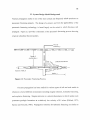
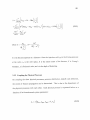
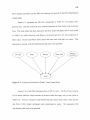
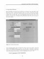
2.3 System Design Model Background
Fracture propagation radius is one of the most critical and frequently asked questions on
pneumatic fracturing projects. The design of a project, and even the applicability of the
pneumatic fracturing technology, is based largely on the extent to which fractures will
propagate. Figure 2.2 provides a schematic of the pneumatic fracturing process showing
a typical subsurface fracture pattern.
Figure 2.2 Pneumatic Fracturing Process.
Fracture propagation has been studied for various types of soil and rock media in
relation to several different mechanisms including magma intrusion, hydraulic fracturing,
and explosive fracturing. Magma intrusion is a natural phenomena in which molten rock
penetrates geologic formations at a relatively low velocity of 0.5 m/sec (Pollard, 1973;
Spence and Turcotte, 1985). Propagation velocities for hydraulic fracturing are similar to
34
those for magma intrusion. Numerous studies of hydraulic fracture propagation have
been conducted due to its importance in the petroleum industry (Perkins and Kern, 1961;
Geertsma and de Klerk, 1969). Explosive fracturing, which causes much higher
propagation velocities (approximately 330 m/sec and greater), has been applied to
enhance the permeabilities of oil, gas, and geothermal wells (Nilson el al., 1985).
Pneumatically induced fractures propagate at velocities which are intermediate
between the previously cited mechanisms. A unique aspect of pneumatic fracture
propagation is the profound influence of formation leakoff owing to the lower viscosity
of the fracturing fluid. The effects of leakoff have been modeled during a recent study at
CEES (Puppala, 1998). This model serves as the basis for the algorithmic logic used in
the System Design component of PF-Model. The approach is developed around the
coupling of three physical processes controlling propagation:
•
pressure loss due to frictional effects,
•
leakoff into the surrounding formation, and
•
deflection of the overburden.
Pressure loss is modeled based on Poiseuille's law, leakoff is modeled using twodimensional Darcian flow, while deflection is modeled as a circular plate clamped at its
edges and subjected to a logarithmically varying load. These processes and their
coupling are discussed in detail in Section 3.3, "System Design Approach."
CHAPTER 3
PROGRAM AND MODEL APPROACH
3.1 Overview of Concept and Model Components
In order for technologies to advance from the research arena into the industrial sector,
they must undergo the process of technology transfer. The "leap" of technology transfer
is an important, yet difficult link to accomplish. Pneumatic fracturing is receiving
considerable industrial attention since it addresses a problem which has plagued
environmental clean-up efforts to date, i.e., remediation of low permeability geologic
formations. It is clear, then, that the computer model greatly enhances the technology
transfer of pneumatic fracturing by linking together the results of numerous laboratory
studies, pilot field demonstrations, and analytical modeling studies. Figure 3.1 on the
following page illustrates the conceptual role of the computer model in the technology
transfer of pneumatic fracturing.
PF-Model is a WindowsTM format program which is interactive with the user.
The program contains a data library (i.e., the knowledge base) of geoteclmical
probabilities related to pneumatic fracturing based on previous experience and expert
knowledge. It also contains an extensive default library which is calibrated to previous
site data. PF-Model allows potential users to add proprietary data generated by future
projects into the knowledge base and default library. A nominal amount of format
detailing is incorporated for user convenience. The program has two principal
35
36
Figure 3.1 Conceptualization of the Technology Transfer Process.
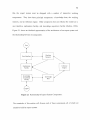
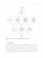
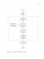
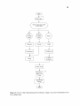
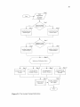
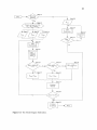
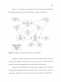
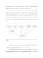
components: Site Screening and System Design. Figure 3.2 on the following page is a
"top level" flow chart showing the model component's interactions and outputs. The
dashed lines in Figure 3.2 represent areas of future research.
This section will introduce these model components. Discussion of the design
approach for Site Screening and System Design are detailed in Sections 3.2 and 3.3,
respectively. The Calibration Mode (Section 3.4) follows. The chapter will conclude
with a description of the program language and structure (Section 3.5).
37
Figure 3.2 Top Level Flow Chart Showing the Model Components.
3.1.1 Site Screening
This component incorporates data collected from pneumatic fracturing projects to date,
and new data can be added as it becomes available. The needed input data for a site
screening analysis was previously discussed in Section 2.2.1, "Geotechnical Properties."
They include formation type, depth, relative density, consistency, plasticity, fracture
38
frequency, weathering, and water table depth. These data are modeled as expert heuristic
knowledge, i.e., knowledge that cannot be quantified, in PF-Model's knowledge base.
To activate this model component, the user must first enter any known or
estimated geologic properties for a prospective site. The program then compares the
inputted information with the knowledge base. Based upon the results of these
comparisons, a semi-quantitative applicability rating will be assigned for the prospective
site. The programming methods to reach this decision will be based largely on expert
systems.
3.1.2 System Design
The ability to initiate and propagate pneumatic fractures is a function of the
geomechancial properties of the formation, as well as the depth of overburden. A model
for predicting pneumatic fracture initiation and maintenance pressure has been developed
at HSMRC by considering the geologic medium to be brittle, elastic, and
overconsolidated (King, 1993). A model study describing fracture propagation behavior
is also available (Puppala, 1998). These two studies form the basis of the fracture
propagation component of PF-Model.
Most often the System Design component will be used in a "Fracture Prediction
Mode" which is activated when the user enters the system parameters and site geological
properties. The system parameters which influence fracture propagation are the injection
flow rate and well radius. The key geologic properties which must be input into
PF-Model to analyze fracture propagation are modulus of elasticity, cohesion, soil/rock
density, and depth of overburden. If the user is unable to determine these key parameters,
39
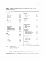
or if they are unavailable, the computer program provides default values. For the system
parameters the program defaults for flow rate and well radius are 1500 scfm and 0.25 in.,
respectively (although some flow rates may vary based on formation type, i.e., typically
100-200 scfm higher in rock). For the geotechnical properties, the default values are
based largely on a general textural description of the geologic materials at the site, e.g.
silty sand, clayey silt, shale, etc. For example, if the site formation is sandstone, but no
tests were performed to determine the rock density, the user could allow the computer
program to use the default value, in this instance 140 lb/ft 3 . Default values for the 14
geologic formation types supported by the program are given in Appendix D.
3.1.2.1 Calibration Mode: Another important function of PF-Model's System Design
component is the "Calibration Mode." In this mode, the post-fracture Young's modulus
and pneumatic conductivity can be estimated if a pilot test has been performed at a site.
Evidence and system data are entered just as in the Fracture Prediction Mode, and after a
series of calculations, the estimated modulus and conductivity can be updated as known
evidence for the Fracture Prediction Mode. This allows for a more accurate estimate of
fracture extent. This mode is detailed further in Section 3.4, "Calibration Mode."
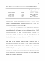
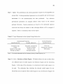
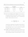
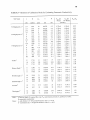
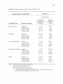
3.1.2.2 Consistency and Strength of Clay Soils: As discussed in Section 2.2.1, the
consistency of fine-grained soils is used as a piece of evidence in the expert system.
However, consistency also plays a major role in the System Design component. The
pneumatic conductivity and modulus of fine-grained formations vary according to
40
consistency. Therefore, PF-Model will select different default values based on formation
type and consistency, thereby greatly affecting the final estimated aperture and radius.
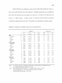
It is advantageous, then, to expand this system utility (i.e., Relative
Density/Consistency) to include other descriptors. At times, field data may be available
in the form of SPT penetration, visual description, or unconfined compressive strength,
q u . The relationship of these descriptors to consistency is shown in Table 3.1. In
PF-Model, this table functions as an interactive system utility, where the user selects the
appropriate descriptor and then PF-Model uses the corresponding consistency.
Table 3.1 Guide to Consistency and Strength of Clay Soils.
41
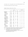
Another descriptor related to consistency, but not as definitive, is the
overconsolidation ratio (OCR). Some users may prefer to describe soil by OCR in lieu of
the descriptors mentioned above. Therefore, the guide shown in Table 3.2 which related
consistency to OCR is also incorporated into PF-Model, but as a subsequent interactive
utility to Table 3.1.
Table 3.2 Approximate Relationship Between Consistency, Consolidation, and OCR.
3.1.3 Future Components
The components of PF-Model can be considered "modules" that can be added or removed
from the main program at any time. Therefore, future model components can be added at
a later date as research progresses. Two components which are currently planned include
Supplemental Media Injection and Contaminant and Transport Analysis, and these are
discussed briefly below.
Supplemental Media Injection. In some pneumatic fracturing applications, liquid or
solid supplements are injected into the formation during the fracturing process to enhance
in situ treatments (e.g., bioremediation, reactive media injection), or for the purposes of
42
mechanical propping. For example, during a recent U.S. EPA SITE Emerging
Technology Project by HSMRC (U.S. EPA, 1995), liquid nutrients and buffer solutions
were injected into fine-grained soils at a refinery site to enhance bioremediation of
gasoline contamination. Thus, there is a clear need for development of a mathematical
model to predict the distribution of supplemental media for various flow rates and
injection times into the subsurface. Once developed, it can be added into the computer
model.
Contaminant Transport Analysis. After a geologic formation has been pneumatically
fractured, the ability to treat and/or remove contaminants depends on the flow and
transport characteristics of the fractured medium. Once a fracture network is established
in a formation, contaminants are more easily accessed since the diffusive distances are
shortened. A one-dimensional solution for a single discrete fracture is currently available
(Ding, 1995). Work is underway to extend this to multiple fractures, and this component
can be added at a later date.
3.2 Site Screening Approach
The general approach to the site screening model was to implement an expert system that
establishes the applicability of pneumatic fracturing for a particular site. Figure 3.3
depicts a flow chart of the site screening model component in which the dotted box
represents the tasks and actions performed by the expert system.
43
Figure 3.3 Flow Chart of Site Screening Component.
44
The critical aspect of any expert system is the selection of which uncertainty
theory to use, which is strongly dependent on the problem domain and any existing
conditions. For reasons discussed in Chapter 2, it was determined that subjective
probability theory is the most appropriate for PF-Model since it has outperformed the
other competing theories (Wise and Henrion, 1986) and experts were available for
technical conversations. Forward chaining acts as the control strategy of PF-Model's
expert system since the pneumatic fracturing process starts out with pieces of geological
evidence proceeding toward a single conclusion, i.e., the applicability of the pneumatic
fracturing technology.
The probabilities that are required to determine pneumatic fracturing applicability
ratings are stored in the knowledge base. Table 3.3 on the following page shows the
assigned probabilities in the knowledge base for permeability enhancement. The
probabilities for dry and liquid media injection are located in Appendix E.
The probabilities for the three different technology variants were established
through discussions with pneumatic fracturing experts over a period of months. The
dominant consideration was past performance of pneumatic fracturing under a variety of
geologic conditions. Careful attention was given to the "relative scale" of probabilities
between the various formations, as well as the "absolute scale" which acknowledged the
importance of a particular type of evidence. It is noted that field reference data are
limited and some probabilities are speculative based upon the inherent geotechnical
properties of a particular formation.
45
Table 3.3 Assigned Permeability Enhancement Probabilities for the Site Screening
Component of PF-Model.
Note that for certain formation types, some geotechnica.l properties may not be
applicable as evidence. For example, if the formation is a silty sand, the only applicable
46
geotechnical properties are depth (for soils), relative density, and water table. It is
therefore the task of the inference engine to determine which probabilities are applicable
and which rules are to be fired.
The rules to be fired can be categorized by their overall interactions. Since some
of the geotechnical properties listed in Table 3.3 apply to certain types of formations (i.e.,
only clay soils exhibit plasticity), while other properties had different states for the
categorized formations (i.e., the states of depth for soil and rock are different),
interpretation by the inference engine is difficult. Therefore, in order to minimize
internal code, processing time, and logic, the geologic formations are arranged into three
different categories which are accessed separately by the inference engine. These are
shown in Tables 3.4 to 3.6 which follow.
Table 3.4 Geologic Properties that Apply to Fine-Grained
Soils (Clay, Clayey Sand, Clayey Silt, Silty Clay).
47
Table 3.5 Geologic Properties that Apply to CoarseGrained Soils (Silt, Silty Sand, Sand, Sand & Gravel,
Gravel).
Table 3.6 Geologic Properties that Apply to Rocks
(Shale/Siltstone, Sandstone, Limestone/Dolomite,
Granite/Gneiss/Schist, and Basalt).
Figure 3.4 on the following page is a flow chart that shows how the inference
engine will access each probability from the knowledge base. By examining the flow
48
Figure 3.4 Flow Chart Representing How Inference Engine Accesses Probabilities From
Knowledge Base.
49
chart, it can be seen that the model obtains evidence and then proceeds toward a desired
goal (i.e., forward chaining).
Figure 3.4 also shows the step in the heuristic process where the inference engine
determines the rules that are to be fired (refer to the "*" in the figure). As pointed out
previously in Chapter 2, the selection of the rule and the uncertainty theory used is the
most important aspect of the inference engine, and the discussion which follows will
provide a clearer understanding of the implementational logic used.
In order to clarify the implementational logic (or which rules are fired) in the
inference engine, it is advantageous to change the terms A and B of Equation 2-2. In
subjective probability, if we let p(H) be the prior probabilities of all possible hypotheses,
and p(E|H) be the conditional probabilities for observing a piece of evidence given a
hypothesis, Equation 2-2 can be rewritten in terms of /I and E. This yields:
Initially, the user will give the system information about characteristics of the site (i.e.,
The Site Screening component of PF-Model has two hypotheses; pneumatic
fracturing is applicable and pneumatic fracturing is not applicable. There is also the
possibility that numerous pieces of evidence are available. In order to account for both
multiple hypotheses and multiple pieces of evidence, Equation 3-1 can be generalized in a
50
manner proposed by Ng and Abramson (1990). This is accomplished by first considering
a single piece of evidence with multiple (mutually exclusive and exhaustive) hypotheses.
The relation becomes:
For multiple evidence and multiple (mutually exclusive and exhaustive)
hypotheses, the following is obtained:
In order to simplify Equation 3-3, conditional independence can be assumed
among the pieces of geological evidence given the hypothesis. Therefore,
This is the general equation used by the inference engine in determining the
applicability of pneumatic fracturing in the Site Screening component.
Appendix F contains an illustrative example of how subjective probability theory
is used to perform site screening. The example shows how various pieces of evidence
51
such as grain size, overburden, and plasticity result in a belief for the applicability of
pneumatic fracturing.
3.3 System Design Approach
Over the years, there has been extensive research in the field of pneumatically induced
fractures and its controlling physical processes. Recent efforts by Puppala (1998) have
led to the development of a mathematical model that determines the radius of pneumatic
fractures in soil and rock formations. This section will present the background
information leading to the final conclusions of that study regarding fracture propagation,
followed by a detailed discussion of PF-Model's System Design algorithm.
3.3.1 Physical Processes
There are three physical processes that control pneumatically induced fractures. They are
pressure distribution, leakoff, and deflection. These three processes are coupled to
predict the radius of fracture propagation. This section briefly discusses each of the three
models.
Pressure Distribution Model. A model has been developed at NJIT that defines the
relationship between air flow and artificially induced fractures (Nautiyal, 1994). The
model accounts for the pressure dissipation in a fracture which states that as radial
distance increases from the injection well, pressure head decreases within the fracture.
The solution is based on Poiseuille type flow between two infinite, smooth parallel plates
and is given by:
52
where 0 is the potential function, U is the velocity of the fluid, At is the dynamic viscosity
of the fluid, and p is the fluid's density. Accounting for compressibility and solving the
differential equation yields:
where p n and p n+1
are pressures at distance r n and rn+1 respectively, 0 is the flow
between rn and rn + 1, b is the fracture aperture, and g is acceleration due to gravity.
Leakoff Model. Fracture propagation is also affected by leakoff, the physical process
where gas escapes from the fracture plane and into the formation. Leakoff is modeled in
three dimensions to account for pressure variations with respect to the distance from the
injection well. Formation anisotropy and fluid losses at the fracture tip are also
considered. The leakoff model uses two approaches to predict the complex pattern of
leakoff that occurs in a fracture: a graphical method and an analytical method.
53
In the graphical (or flownet) method, Darcy's law is modified to account for the
variation in leakoff with radial distance. Darcy's equation for two-dimensional flow is
given as:
where ()l ea k is the air flow lost, Kgas is the effective pneumatic conductivity of the
formation, H is the total head driving the flow, Nf is the number of flow tubes, and Nd is
the number of potential drops.
To account for pressure variation with respect to radial distance, the length of the
fracture is divided into 'n' segments and then the number of flow tubes leaving each
segment is counted. The leakoff occurring in each segment can then be computed as:
where r w is the well radius, R is the final fracture radius, and Hn
is the total head driving
the flow in the nth segment.
By further segmenting the radial fracture into concentric annular rings, the
formula for total leakoff in three dimensions can be derived as:
54
where r n is the inner radial distance and r n+1 is the outer radial distance of the annular
ring.
The analytical method calculates leakoff by summing the lost flow from
successive annular rings of the fracture surface. This is given by:
where Kh-gas and Kv_ gas are respectively the horizontal and vertical pneumatic
conductivities of the formation, pd is the driving pressure, and !gra d is the flowpath
length along which the pressure is dissipated along the n th segment.
Deflection Model. It is assumed that pneumatic fractures are due to overburden
deflection which is a function of the pressure distribution within the fracture (Canino,
1997). A model to predict the overburden deflection was investigated which uses a nonlinear distribution to predict a tapering fracture (Canino, 1997 and Puppala, )998).
Field observations have shown ground surface heave contours circular in shape.
Therefore, overburden can be modeled as the bending of an elastic circular plate clamped
at the edges. The derived "deflection" equation is:
55
b is the fracture aperture at a distance r from the injection well, Pd is the driving pressure
at the well, r w is the well radius, R is the radial extent of the fracture, E is Young's
Modulus, v is Poisson's ratio, and z is the depth of fracturing.
3.3.2 Coupling the Physical Processes
By coupling the three physical processes, pressure distribution, leakoff, and deflection,
the extent of fracture propagation can be determined. This is due to the dependency of
the physical processes with each other. Each physical process is expressed below as a
function of its formation and system parameters:
56
The above equations demonstrate this interdependency, since each dependent variable
appears within one of the other processes' list of independent variables. This coupling of
the physical processes is handled with an algorithm that is described in the following
section.
3.3.3 System Design Algorithm
The System Design algorithm is represented by three nested subroutines. They are the
System Design, Model Engine, and PDF Subroutines and are presented in the following
three sections.
3.3.3.1 System Design Subroutine: This is the "top level" of the System Design
algorithm. The subroutine is shown in Figure 3.5 on the following page. In this
subroutine, many of the initializations and preparations of data required in the later
subroutines are carried out as detailed in the following discussion.
57
Figure 3.5 The System Design Subroutine.
58
Step I - Input. The geotech ical and system parameters required by the algorithm are
n
entered first. Certain geotechnical parameters are site specific and will be known
beforehand if a site characterization has been performed. Any unknown
geotechnical parameters are assigned default values based on the selected
geologic formation. System parameters are based on the anticipated injection
event and can always be entered as data, although defaults will be assigned if
required. Table 3.7 summarizes these various inputs.
Table 3.7 Input Parameters for the System Design Subroutine.
Steps 2, 3, & 4 - Selection of Model Engine. PF-Model allows the user to select from
two different types of model engines: the Bisection Engine and the Increasing
Engine. In this step of the subroutine, it is determined which model engine is to
be used. The subroutine then initializes the selected model engine for use.
Should the user not specify which model engine to run, the Bisection Engine will
59
be used as the default. The discussion of the two model engines is presented in
the following section, the Model Engine Subroutine.
Steps 5, 6, & 7 - Selection of Leakoff Method. In this step the method of leakoff is
selected, which can be either the graphical method or the analytical method as
discussed previously in Section 3.3.1, "Geophysical Processes." The graphical
method is based on the construction of a flownet and obtaining the "shape factor"
associated with it. Appendix G contains the shape factors used as the default in
PF-Model's advanced menu function, Flownet Parameters. As this method is
believed to give the most accurate representation of leakoff within a fractured
formation, it will be the default should the user not specify a leakoff method.
The other method is the analytical method as described by Equation 3-10.
The difference in this method is that an "effective" pneumatic conductivity must
be used when calculating leakoff in anisotropic formations. It is therefore simpler
than the graphical method, but less accurate since variations in gradient and
formation anisotropy are not accounted for.
Steps 8 through 12 - Selection of Deflection Solver Method. In PF-Model, four
Deflection Solvers are available, each with a different fracture aperture geometry.
After the user selects the desired Deflection Solver, the subroutine then prepares
the Solver to be passed to the PDF Subroutine. Table 3.8 lists the four Solvers
and the corresponding equations.
60
Table 3.8 Deflection Solvers and Corresponding Equations.
The choice of Deflection Solver has a significant effect on the estimated fracture
radius. Regressive analyses have shown that the equation for bending of a
circular plate fixed at its edges best approximates field results (Canino, 1997).
Therefore, the circular plan fracture and log pressure distribution will be the
default selection in PF-Model.
61
Step 13 - Model Engine Subroutine. At this point in the System Design Subroutine,
control is passed to the Model Engine Subroutine which is discussed in the
following section.
Step 14 - System Design Output. When control is passed back from the Model Engine
Subroutine, the final output is then presented to the user. The fracture radius and
aperture that satisfy the flow and pressure conditions are presented in numerical
form, while aperture width, residual flow, and pressure distributions within the
fracture as a function of radial distance are presented in graphical form.
3.3.3.2 Model Engine Subroutine: This subroutine controls the associated logic of the
Bisection and Increasing Model Engines which are selected by the user during the System
Design Subroutine. Figure 3.6 on the following page shows the logic of the Model
Engine Subroutine.
The Bisection Model Engine (Steps 16 through 28) is based on the method of
bisections (also known as binary chopping, interval halving, or Bolozano's method).
This method has the ability to substantially reduce the number of iterations and
processing time required, which is why this method is preferred and is the default engine
for PF-Model. The method of bisections works by dividing the interval in half, and then
determining in which half the root resides. The selected interval is halved again, and the
process repeats itself until the root converges to zero. At this point the fracture radius has
attained its maximum value.
62
Figure 3.6 The Model Engine Subroutine.
63
The Increasing Model Engine (Steps 20, 30 through 32) is the alternative to the
Bisection Engine. The increasing method starts at the smallest radius (Le., the well
radius) and increases until the pressure and continuity conditions at the fracture tip are
satisfied during the same segment of the subroutine. This is repeated for each increment
in radius. Therefore, when the fracture radius extends past 7 ft, the processing time can
become quite lengthy.
The steps involved in the subroutine are presented below.
Step 15 - Engine Selection. When control of the algorithm is passed to this subroutine, it
passes which model engine has been selected. This step determines which
subsequent logic to follow: bisection or increasing. If Bisection is selected, the
subroutine proceeds to Step 16. Otherwise, the subroutine proceeds to Step 30 for
the Increasing Engine.
Steps 16 through 19 - Radius Initialization. The initialization of the upper and lower
bounds of the radius interval are chosen such that the actual radius lies within this
interval. From experience, the lower limit, RLow, is chosen to be the well radius
(in most cases, 0.25 ft). For the upper limit, RHigh , a value of 200 ft is selected.
Next, the value of RMid
is prepared, which is:
64
All three values are then passed as input to the PDF Subroutine which
processes the values as a parallel operation in logic.
Step 20 - PDF Subroutine. The PDF (or Pressure, Deflection, and Flow) Subroutine is
passed control with values of the radii determined in the Model Engine
Subroutine. The PDF Subroutine is discussed in Section 3.3.3.3.
Step 21 - Internal Storage of PDF Subroutine Results. As control passes back to the
Model Engine Subroutine, the results of the PDF Subroutine are stored internally
for later comparison using the bisection method.
Steps 22 through 26 - Flow Function and Interval Determination. The results held in
the internal storage (Step 21) are compared in order to determine the location of
the radius along the entire interval. The comparison is shown in Table 3.9 along
with the actions the Bisection Engine is to perform.
Table 3.9 Rules, Interval Determination, and Actions for the Bisection Engine.
65
Steps 27 and 28 - Error Calculation and Error Comparison. These steps determine if
the actual radius, given the current iteration's flow and pressure conditions, has
been reached. First, the relative error is calculated as:
Equation 3-16 can be simplified further by making the following substitutions:
therefore giving as the relative error,
As long as this error is greater that 0.1%, the Bisection Engine will pass control
back to the PDF Subroutine (Step 20) with new values for RLow, R Mid,and
RHigh (determined from Steps 25 and 26). If the error is less that 0.1%, the
subroutine has converged on the radius and proceeds to Step 29.
66
Step 29 - Output. Upon reaching this step in the subroutine, the values for the aperture
and radius, as well as subroutine control, are passed back to the System Design
Subroutine (Step 13).
Step 30 - Input Radius, Increasing Engine. The input radius for the Increasing Engine
starts at the value of the well radius (usually 0.25 ft). This value is then passed to
the PDF Subroutine (Step 20).
Step 31 - Flow Comparison. Should the PDF Subroutine return a flow value less than
zero, then the actual radius has been reached and the subroutine proceeds to
provide the output (Step 29).
Step 32 - Increment Radius. If the value of Q(RLow) from Step 31 is greater than zero,
the radius RLow is incremented by 0.1. This value is then passed along with
control back to the PDF Subroutine (Step 20).
3.3.3.3 PDF Subroutine (Pressure, Deflection, and Flow): This section outlines the
logic of the PDF Subroutine which is presented in Figure 3.7 on the following page.
When the fracture radii (RLow , RMid, and RHigh) are passed to this subroutine, the
fracture extent is discretized into smaller segments. The residual flow, O res , and pressure
distribution at the fracture tip, p, are calculated for this first segment. If the O res is
greater than zero or the pressure at the tip is greater than the propagation pressure, "'prop ,
the algorithm steps the radius incrementally. This process continues until the three
controlling conditions, elastic form, pressure distribution, and formation leakoff, which
correspond to the calculations of Steps 36, 37, and 39 respectively, are satisfied. These
three steps, as well as the others that make up the PDF subroutine, are discussed below.
67
Figure 3.7 The PDF Subroutine (Pressure, Deflection, and Flow).
Step 33 - Discretize the Fracture Radius. The fracture radius is discretized into a
number of segments equal to R/rincr ,wher incr isdefinedas:
68
Step 34- Calculate Propagation Pressure. The pressure required to propagate fractures,
pprop , is given by:
where p m is the maintenance pressure and Pk is the pressure required to overcome
fracture toughness. A semi-empirical relationship is available for estimating
maintenance pressures in the saturated zone is given by (King, 1993):
where λ . is a coefficient, z is the depth of the fracture, z w is the depth to the water
table, γ is the bulk weight of the formation, and γwisthepcfgoatr.
If the fracturing occurs in the vadose zone, the above equation reduces to:
In the Fracture Prediction Mode, the user will rarely know the
maintenance pressure, so instead the program performs the computation and
69
provides a default value. For simplicity, Equation 3-22 is used for both the
vadose and saturated zones, although if fracturing in the latter, the coefficient, A,
is increased by 1.0. This adjustment accounts for the superior "seal" and heavier
weight of the saturated formation. Note that this adjustment would not apply if
multiple injections have dewatered the formation.
In addition, prior research has shown that maintenance pressure increases
with increasing flow rate (Heres, 1994). A regression of available data yielded the
values of the coefficient, A, shown in Table 3.10. Examination of Table 3.10
shows that for flow rates above 1600 scfm, the coefficient increases linearly by
10% (thereby corresponding to a 10% linear increase in maintenance pressure) for
each 500 scfm increase in flow rate.
Table 3.10 The Coefficient, 2, for Soil and Rock Formations Varying with
Injection Flow Rate.
70
The value of the pressure, Pk, required to overcome fracture toughness is
where Ki c is the formation's fracture toughness and r is the fracture radius.
Steps 35 & 36 - Aperture Calculation. The Deflection Solver selected previously during
the System Design Subroutine (Steps 8 through 12) is called from internal storage
(Step 35) and is now used to calculate the aperture (Step 36). Table 3.8, shown
previously, summarizes the equations used for each deflection model in the
Deflection Solver.
Step 37 - Pressure Distribution Calculation. After the aperture has been calculated, the
pressure model of Section 3.3.1 is solved. The pressure distribution in the current
segment is calculated using Equation 3-6, which is repeated below:
71
density of the injected gas, b is the fracture width, and g is the acceleration due to
gravity.
Steps 38 & 39 - Leakoff and Residual Flow Calculations. The next step in the PDF
Subroutine is calculation of the residual flow, O res . This is done by first
calculating the leakoff from the fracture, Qleak. One of the two leakoff methods
determined during the System Design Subroutine (Steps 5 through 7) is called
from internal storage (Step 38). The related equations were discussed previously
in Section 3.3.1, and are repeated below for convenience. For the graphical (or
flownet) method, leakoff is given by:
found by determining the overall mass-balance of the flow. Ignoring fracture
volume,
72
where O res. , _, is the residual flow of the previous segment, and Q leakn is the
leakoff flow loss of the current segment. This step of the subroutine satisfies the
leakoff model discussed in Section 3.3.1.
Step 40 - PDF Criteria Comparison. Residual flow, fracture pressure distribution, and
radius at the end of the segment are compared to the conditions that would exist at
the fracture tip if in equilibrium, as shown in Step 40 of Figure 3.7. If this
condition is satisfied, control passes to Step 41, otherwise, execution is passed to
Step 42.
Step 41 - Increase the Segmentized Fracture Radius. If the conditions of equilibrium of
Step 40 are satisfied, then the discretized fracture radius is increased by r incr given
by:
where rn +1 is the new segmental fracture radius, rn is the segmental fracture
radius for the current iteration, and rincr is the size of the incremental radius
which was defined previously in Equations 3-18 and 3-19.
Execution then passes back to Step 36 where the current values for
residual flow and pressure are used as the input for the next segment about to be
executed.
73
Step 42 - Output. The values of residual flow, aperture, propagation radius, and pressure
are returned along with the process control back to the System Design Subroutine
if the conditions of Step 40 are not satisfied. Control is passed if and only if all
three conditions are not satisfied, which corresponds to the convergence of all
three physical processes and indicates that the final propagation radius has been
reached.
3.4 Calibration Mode
A "Calibration Mode" was implemented into PF-Model to aid in analysis of field pilot
tests during the site characterization phase of a project. In this program mode, actual
field measurements of ground surface heave are input into PF-Model to regress the actual
post-fracture Young's modulus and pneumatic conductivity for the formation being
tested. These values are then used directly in the System Design component to design
full scale fracturing for the site. As might be expected, the accuracy of design predictions
made after running the Calibration Mode will be superior to those made without running
it.
3.4.1 Calibration Algorithm
In many ways, the Calibration Mode is similar in logic to the System Design mode
discussed previously. With some minor differences, the same three subroutines of the
System Design mode are nested within the main subroutine of the Calibration Mode.
This is explained in the following section.
74
3.4.1.1 Calibration Subroutine: The subroutine first regresses the post-fracture
Young's modulus, and then uses the method of bisections to converge on the
post-fracture pneumatic conductivity of the site.
The method of bisections was chosen as the model engine for processing speed
considerations due to the fact that the Calibration Subroutine converges on two solutions
in two separate intervals (i.e., the pneumatic conductivity and the corresponding residual
flow rate that satisfy the conductivity in the current iteration). The method of bisections
keeps the processing times to a manageable level. Figure 3.8 on the following page
shows the steps involved in the Calibration Subroutine and an explanation of the figure
-
follows.
Step 1 - Data Input. The system properties from the pilot test, i.e., the depth of
fracturing, injection flow rate, and maintenance pressure, are entered with the
resulting measured aperture and radius of fracture. Other properties (i.e., unit
weight, Poisson's ratio, etc.) can also be entered if known, or PF-Model can
assign the default values instead.
Step 2 - Regress Modulus. Deflection of the overburden can be modeled by assuming
the bending of an elastic circular plate that is clamped at its edges with a
logarithmically varying load. In this step the Young's modulus for the formation
is calculated by manipulating Equation 3-11 into a more useful form. Based on
75
Figure 3.8 The Calibration Subroutine.
76
the maximum measured radius, R, and the maximum measured ground heave at
the well, b 14) , it is possible to solve for Young's modulus, E, as follows:
Steps 3 through 6. The initialization of the upper and lower bounds of the post-fracture
pneumatic conductivity interval are chosen such that the actual conductivity lies
within this interval. The lower limit, KL ow , is chosen to be zero. For the upper
limit, KHigh, a value of 100 ft/day is selected. Next, the value of KMid is
prepared, which is:
All three values are then passed as input to the Composite Calibration
Subroutine which processes the values as a parallel operation in logic.
Step 7 - Composite Calibration Subroutine. The Composite Calibration Subroutine (or
CC Subroutine) receives its name in that it contains the three subroutines found in
the System Design component, but with three major differences. The first is that
only the method of bisections is used as the Composite Calibration Subroutine's
77
model engine. Second, the Deflection Solver in the CC Subroutine is the circular
plan fracture subjected to a logarithmically varying load distribution. And last,
the Analytical method is used as the leakoff model. It is important to note that
this deviates from the Fracture Prediction Mode of PF-Model, which uses the
Graphical method as a default. The Analytical method is considered more
appropriate for the Calibration Mode since in virtually all instances the actual
field results will yield an effective conductivity, Keff.Subseqntflowchard
process descriptions for these subroutines are not provided, since they are
basically the same as those shown in Figures 3.5, 3.6, and 3.7, but with the
obvious modifications as described above.
Step 8 - Internal Storage of CC Subroutine Results. As control passes back to the
Calibration Subroutine, the results of the CC Subroutine are stored internally for
later comparison.
Steps 9 through 13 - Conductivity Function and Interval Determination. The results
held in the internal storage (Step 8) are compared in order to determine the value
of the radius corresponding to the effective conductivity along the entire interval.
The comparison rules and actions to be taken are shown in Table 3.11 on the
following page. Note that the functions (R(KLow ), etc.) are returning radius
values which are based on the conductivity of the current iteration. If one of the
rules are true, the corresponding action to update the conductivity is then executed
(i.e., set KHigh = KMid, etc.).
78
Table 3.11 Rules, Interval Determination, and Actions taken for the Calibration Mode.
Steps 14 and 15 - Error Calculation and Error Comparison. These steps determine if
the actual effective conductivity has been reached. The relative error is calculated
in a similar manner as presented in Equations 3-16 and 3-17 of the Model Engine
Subroutine. Therefore, the relative error is given by:
As long as this error is greater that 0.1%, the subroutine will pass control back to
the CC Subroutine (Step 7) with new values for K Low, KMid, and KHigh
(determined from Steps 12 and 13). If the error is less that 0.1%, the subroutine
has converged on the effective conductivity and executes Step 16.
Step 16 - Output. Upon reaching this step in the subroutine, the post-fracture values for
Young's modulus, E, and effective pneumatic conductivity, Keff, are returned.
These values represent an estimation of the actual field conditions. Now, instead
79
of using default values for E and Keff in the System Design component, these
values can be used.
3.5 Program Language and Structure
Several application development tools were available for development of PF-Model and
include, Borland C I I Builder, Borland Delphi, IBM VisualAge C++, Microsoft Visual
C++, and Microsoft Visual Basic. Although these development tools can create powerful
and robust applications, many are aimed at different audiences. For example, Visual
Basic is aimed at developers who are using Microsoft products exclusively.
These development tools each have different features, and therefore exhibit
different advantages over the others. In the instance of VisualAge C++, it uses a
debugger and automatic memory manager, and is specifically designed to improve
programmer productivity through incremental compilation. Even the degree of
sophistication between two development tools aimed at the same audience can vary, such
as Delphi and Visual Basic. Delphi uses Decision Cube components, which help create
local multidimensional data stores that can be summarized into cross-tabulated views and
graphs. Although these cross-tab queries can be created in Visual Basic, Delphi's
Decision Cube can more easily pivot and re-slice the data, allowing the analysis to be
done faster.
Eventually, it was decided to use Microsoft Visual Basic for PF-Model. An
important reason for selecting Visual Basic was to facilitate future modifications and
additions to the program, which are inevitable. Visual Basic allows those students and
80
faculty not proficient in higher level computer languages the ability to access and modify
the program code.
Like the alternative development tools, Visual Basic allows for the creation of
robust and powerful applications for Microsoft Windows operating systems, yet retains
the programming ease of standard Basic. Visual Basic also allows programmers to
incorporate an extensive graphical user interface (GUI) into the program.
A new feature of Visual Basic allows PF-Model to be compiled in native code
similar to the other development tools. This provides for several options for optimizing
and debugging that aren't available in standard pseudo code, or p-code. P-code is
described as an intermediate step between the high level instructions in the actual Basic
program and the low level native code executed by the computer processor. Normally, at
run time, each p-code statement is translated into native code. By compiling to native
code directly, the intermediate p-code step is eliminated, thereby extending performance
up to 20 times faster (Microsoft, 1997).
Another advantage is compiled native code can be debugged with other standard
native code debugging software, such as Visual C++. One can also optimize the native
code for speed or size in any of the other native code debugging software environments
(Microsoft, 1997).
PF-Model is a menu driven (as opposed to command driven) program and this is
apparent when the user runs the program and views the GUI. The GUI for the model
consists of objects, such as "buttons," "arrows," "pull down menus," etc., all familiar to
computer users today. The interface reacts with the user by responding to events that
81
occur in the interface. The user in turn is able to handle otherwise difficult situations
easily and rapidly.
For example, the entry of large amounts of data needed for any application can be
daunting. Needed information may not be available at all times, or it may not be of
significant importance for the application to run and produce results for the user. This is
the situation, for example, in one of PF-Model's advanced functions, "Input Parameters."
The approach for alleviating this potential problem was to have the program select default
values for certain parameters by activating a "button" on the GUI. Thus, with the ease of
a mouse click, default values are entered and the application can return results to the user.
This is particularly useful for the pneumatic fracturing computer model, since detailed
geologic data are not always available for analysis.
The program manual for PF-Model is presented in Appendix H. It contains
various screen shots of the GUI, sample output graphs, and a step-by-step example that
will guide the user through both the Site Screening and System Design components. By
reviewing the manual and working through the step-by-step example, the user becomes
acquainted with PF-Model's menu driven GUI and the various functions available.
A quick examination of either the manual, or the actual program, will show that
the key element in the entire program is the Data Input Screen since it interacts with both
the Site Screening component and the System Design component. The Data Input Screen
stores all the required information needed by the other model components to perform
their functions. The interaction of the data set and the model components allows the user
to easily move from one component to another component within the program.
82
Figure 3.9 is a schematic of the different screens and components of PF-Model,
showing the global interactions of all the components, engines, and data bases.
Figure 3.9 Interaction of Components, Engines, and Data Bases.
Appendix I contains select portions of code used in programming PF-Model, as
the entire code would be too extensive to list as part of this work. The selected code is
included for review of programming style and copyright protection purposes.
Floppy disks of PF-Model can be obtained with a manual from the Center for
Environmental Engineering and Science (GEES) located at the New Jersey Institute of
Technology, 138 Warren St., Newark, NJ, 07102. The phone number is 973/596-2457.
CHAPTER 4
VALIDATION AND CALIBRATION OF PF-MODEL
4.1 Introduction
In order for PF-Model to be useful for consultants, designers, and researchers, it must
provide reasonable results. Since PF-Model has two different components, Site
Screening and System Design, two distinctive evaluation methods will be used.
The approach for evaluating the Site Screening component was system validation
and user acceptance (Section 4.2). The System Design component was verified more
traditionally, i.e., validation and calibration (Section 4.3). The results of each of these
evaluation procedures will now be examined.
4.2 Site Screening
Since the Site Screening component is an expert system, its evaluation differs greatly
from conventional computer programs. In conventional programs, verification is the
major concern since this determines if the program completely satisfies the initial
conditions (Adrion et al., 1982). As discussed previously in Chapter 2, conventional
programs have well defined algorithms and structures, and therefore can be measured
against some objective standard. On the other hand, an expert system is designed to
answer questions heuristically for which there is no right or wrong answer. That is, there
is no "gold standard" against which the performance of the expert system can be
measured absolutely (Gasching et al., 1983).
83
84
Because of the lack of an absolute standard, the Site Screening component was
evaluated using system validation and user acceptance (Preece, 1990). The evaluation
methods are somewhat more relaxed than the stringent verification process that the
System Design component has undergone (see Section 4.3). System validation tries to
determine if the system performs the intended task "satisfactorily" (Hollinger, 1989).
User acceptance evaluates whether the system meets the needs of the user. It is noted that
the procedures of system validation and user acceptance are somewhat subjective, and
therefore make the evaluation of an expert system complex (Durkin, 1994).
4.2.1 System Validation of Site Screening Component
Since the Site Screening component models the decision making process of a human
expert, PF-Model should obtain the same results as the expert. Therefore, the system
validation of the Site Screening component involved the use of test cases. The selected
test cases were based on a blend of actual and hypothetical field experiences which varied
in success. During the validation procedure, the site evidence was given to both the
expert system and several expert "evaluators," and the results were compared.
It should be noted that when the evaluators agree with the system, the results are
viewed as correct, otherwise, they are wrong. This approach assumes that the test case
result is 100% correct and that any different answer is incorrect. This is not necessarily
the case, since the findings represent an expert opinion, not a "gold standard."
The system validation step was based on three major considerations. They were:
85
•
test criterion,
•
test cases, and
•
selection of evaluators.
Test Criterion. The test criterion was selected to directly reflect the Site Screening
component. The applicability of pneumatic fracturing at the sites were rated using three
categories: technology recommended, technology marginal, and technology not
recommended. In addition three different variants of pneumatic fracturing were
evaluated, i.e., permeability enhancement, dry media injection, and liquid media
injection.
Test Cases. Likewise, the selection of the test cases was based on the goal of the Site
Screening component and original objective of the expert system. The test cases were
selected to be typical sites that one expects to encounter in remediation work. It is
believed that if the Site Screening component can make reliable recommendations 80% of
the time for typical sites, the other more difficult sites can be handled by a human expert.
Fifteen different test cases were selected and are shown in Table 4.1. These cases include
common geologic situations for pneumatic fracturing, as well as more challenging
geologic conditions.
Selection of Evaluators. The selection of evaluators was also consistent with the original
goal and objective of the Site Screening component. A total of five evaluators were used
86
for system validation. This included the two experts who were largely responsible for
development of the PF-Model program and whose knowledge the expert system reflects.
In addition, three evaluators were selected from the remediation field who are considered
to be the foremost experts in the relatively new process of pneumatic fracturing.
System Validation Results. The results of the system validation are presented in
Table 4.1 for the permeability enhancement variant, and additional results for dry and
liquid media variants are contained in Tables J.1 and J.2 of Appendix J, respectively. The
first column in each table summarizes the available geotechnical evidence for the test
cases. The results of the five expert evaluators are presented in the second column. Each
evaluator was asked to rate each site as: variant recommended (Y), variant marginally
recommended (M), and variant not recommended (N). Finally, the corresponding expert
system result and technology rating for each case are shown in the last column.
These system results and ratings were determined through an iterative testing
process. Starting with the original knowledge base, the results of the expert system were
compared to the results of the evaluators. If the expert system agreed with the majority
opinion for a selected site, the system results were deemed satisfactory. If the system
differed with the majority opinion, some "fine tuning" of the knowledge base was
required to bring the expert system results into agreement. The expert system was then
reevaluated for each site to insure that the changes to the knowledge base did not alter the
system results elsewhere. This process was repeated until the results in the tables were
obtained.
Table 4.1 System Validation of Permeability Enhancement Variant.
88
The system results in Tables 4.1, J.1, and J.2 show an agreement of 93, 93, and 80
per cent, respectively. This represents an overall average of 89 per cent among the three
pneumatic fracturing variants.
It should be noted that the subscripts shown for certain recommendations in
Table 4.1 represent the original opinion of the expert. It was inevitable that evaluators
would assess each recommendation differently. Therefore, evaluators were also asked to
rate each site numerically (i.e., from 1 to 10). In some instances, it was apparent that the
original recommendation was a "gray" area for the evaluator. In these instances, the
relative "weight" of the rating further defined their opinion, and was adjusted
accordingly.
Although this may seem like an end to system validation, that is not the case. The
Site Screening component of PF-Model, like most expert systems, contains knowledge
that evolves. Therefore, the way the pneumatic fracturing technology is viewed by
experts may change over time. This can be due to a number of factors including
development of new equipment, modifications of existing equipment, change in work
procedures, and even new research results. Conversely, as the expert system is used,
deficiencies may also be discovered. Therefore, the validation of the expert system is a
continuous process.
4.2.2 User Acceptance of Site Screening Component
This is perhaps the ultimate test of an expert system. If the Site Screening component is
not accepted by the end-user, the expert system will then be of little worth. At this point
a base of 50 or more users are expected, including pneumatic fracturing vendors, design
89
consultants, and government regulators. Of course, the final determination of user
acceptance will not be known until after the program is released to the public.
The major issues of user acceptance are:
•
ease of use,
•
presentation of results,
•
clarity of explanations, and
•
system utilities.
Ease of Use. During the development of the technical features of PF-Model, an effort
was made to present the program in an easy to use format since some users are reluctant
to even try new software. Throughout the programming of PF-Model's interface, the
following features were incorporated to make it user friendly:
•
easy one step installation,
•
explanation/help facility,
•
menu and/or command driven GUI.
This was the major reason why the programming language used was Visual Basic,
as discussed previously in Chapter 3. With the click of a mouse button, all program files
will install in the correct folder locations, a technology recommendation can be obtained,
or the explanation facility can be accessed.
90
Different users also prefer different styles of programs. For instance, some users
prefer to work with menu driven programs, others command driven, or even a
combination of both. PF-Model is menu driven, but was designed to be versatile enough
so a user can use only a keyboard (i.e., command driven) if desired.
Presentation of Results. Several different approaches were explored to present the final
technology recommendation of the Site Screening Component. Originally, the
recommendation was simply verbal, e.g., "technology recommended." However, because
subjective probability was used in the inference engine, it was possible to present
technology recommendations numerically, thereby reflecting a quantitative belief in the
result. In addition, an explanation facility was developed to aid in interpretation of the
numeric as discussed in the next section, "Clarity of Explanations."
Another justification for using a numeric was that when a human expert makes a
recommendation, that recommendation is never absolute. Rather, it is an opinion that
contains some degree of uncertainty (for the success of the technology). This can arise
from the user's wish to protect himself legally, or simply from the fact that site geology
-
and geotechnical properties vary greatly over the same site.
Clarity of Explanations. Many expert systems provide the user with explanations on the
reasoning of the system, i.e., "Why does the system require the depth of injection?"
Since it is expected that most users of PF-Model will either be experts or designers with
some geotechnical knowledge, the reasoning of the expert system will normally be
91
apparent. However, should a user require more information, an explanation can be easily
accessed through PF-Model's Help Function.
In the design of the Site Screening component, it was considered critical to
provide an explanation facility for interpretation of the numeric rating. This is intended
to provide a comfort level in the degree of belief by the expert system. The
recommendation rating is broken into three categories, or ranges, and each range has a
corresponding recommendation that the rating falls in, as detailed below:
•
0 to 45 - The technology is not recommended for traditional applications.
•
45 to 60 - The technology is deemed to be marginally effective. Although the
technology may provide some degree of enhancement, a cost to benefit
analysis may be appropriate. Also, it is recommended that further evidence be
acquired to refine the analysis.
•
60 to 100 - The technology is likely to be effective.
System Utilities. Throughout the development of the Site Screening component, human
experts were consulted to determine the system utilities, as well as their design. This
process was done over many months with different pneumatic fracturing experts.
The most important step in this process was to determine which geotechnical
parameters influence the success of pneumatic fracturing. After extensive discussion, it
was determined that the seven geotechnical properties detailed in Chapter 2 (i.e.,
formation type, depth, plasticity, etc.) have the greatest influence on the pneumatic
92
fracturing process. Further discussions led to the following conclusions about these
properties:
•
formation type was the most important property to effect pneumatic fracturing
and therefore should always be required as input data for the expert system,
•
a hierarchical order was established for the remaining geotechnical properties,
and
•
the geotechnical properties are independent of each other.
The importance of formation type and the other geotechnical properties, as
applied to pneumatic fracturing, was previously discussed in Chapter 2. The hierarchical
order of the geotechnical properties is shown below in Table 4.2 and are grouped
according to soil or rock type.
Table 4.2 Hierarchical Order of Geotechnical Properties.
These geotechnical properties in turn were divided into qualifiers, in order to
quantify the geological evidence for analysis by the expert system. This was done in
93
subsequent discussions with human experts. Table 4.3 below shows how the
geotechnical properties were qualified.
Table 4.3 Breakdown of Geotechnical Properties Into Qualifiers.
Once the geotechnical properties were firmly established, a system utility to
access this information was developed for an early version of PF-Model. This utility was
94
subsequently evaluated by experts for ease of use, understanding, and visual aesthetics.
After some minor GUI modifications, the final system utility was coded.
Finally, it was decided to create a system utility that would give users access to
the knowledge base. This approach allows the expert system to be updated as the
technology evolves and also permits licensed technology vendors to create a knowledge
base with their own proprietary data. It should be noted that if the knowledge base is
modified and multiple experts are not consulted, the expert system may in effect become
insular, and therefore would not truly represent the consensus of expert opinion for the
technology.
4.3 System Design
As opposed to the heuristic structure of the previous section, the System Design
component is programmed with structured algorithms. Therefore, validation and
calibration of this component is relatively straight forward. The validation step confirms
that the model is reasonably representative of the pneumatic fracturing process, while the
calibration step establishes the necessary coefficients and default values to insure proper
functioning of the model. PF-Model was subjected to both these procedures.
Currently, with over 40 sites pneumatically fractured to date, a reasonable data
base exists for validation and calibration purposes. The sites selected for validation and
calibration were previously screened (Puppala, 1998) to insure that sites of only
acceptable data quality were used in the evaluation process. Six different sites were
selected, three involving soil formations and three involving rock formations. The field
data for these sites are presented in the tables throughout this section.
95
It should be noted that PF-Model will continue to be calibrated as future sites are
further added to the data base.
4.3.1 Validation of the System Design Component
The System Design component was validated by comparing PF-Model's predicted results
with actual field results. This approach confirms that PF-Model represents the currently
established fracture propagation mathematical models. Since the System Design
component has two modes of operation, the Calibration Mode and the Fracture Prediction
Mode, two separate validations were done. The results are presented in the following two
sections.
4.3.1.1 Validation of Calibration Mode: As previously discussed, the Calibration
Mode regresses the post-fracture Young's modulus and pneumatic conductivity from
actual field data. Therefore, successful validation of the Calibration Mode will require
agreement of these two geotechnical parameters with the results from the original
mathematical model.
Table 4.4 on the following page shows the results for the validation of Young's
modulus. The first two columns summarize the site data. The third column consists of
two values. The first is a "back calculation" of Young's modulus, E bc. That is, the
observed field radius and aperture were used to back calculate the modulus for the given
site. The calculation of Eb c was performed using the mathematical model in conjunction
with Mathcad Plus 6.0, a technical calculation program. The second value, ,iEpsthfe
96
Table 4.4 Validation of Calibration Mode for Estimating Young's Modulus.
97
estimated post-fracture modulus determined by PF-Model's Calibration Mode. If both of
these results agree, then the post-fracture modulus is adequately represented. This is
indicated in the last column which is the ratio of Eb c/Epf. As can be seen, the modulus
ratio ranged between 1.00 or 1.01 confirming that the Calibration Mode of PF-Model is a
valid representation of the mathematical model in estimating post-fracture Young's
modulus.
The validation of the post-fracture pneumatic conductivity is shown in Table 4.5
on the following page. Again, the first two columns represent the site data, while the
third column lists values of post-fracture pneumatic conductivity, Kmc and Kpf, which
have been calculated using Mathcad and PF-Model, respectively. The final column gives
the ratio, K mc/Kpf, which ranged from 0.94 to 1.06. The average of all the sites was
0.99, thus demonstrating reasonable agreement. It is surmised that the slightly higher
variation in the ratio K mc/Kpf is related to how Mathcad and PF-Model handle significant
figures. Since the convergence algorithm consists of thousands of iterations, any
difference in significant figures is compounded as the algorithm propagates, thereby
creating the higher variation.
4.3.1.2 Validation of Fracture Prediction Mode: The Fracture Prediction Mode
estimates the maximum fracture radius and aperture upon inputting geological and
operational data. Therefore, in a manner similar to the Calibration Mode, successful
validation requires agreement between PF-Model and the original mathematical model.
98
Table 4.5 Validation of Calibration Mode for Estimating Pneumatic Conductivity.
99
Table 4.6 on the following page shows the validation of the graphical leakoff
method (where K h = 5KV ) using the bisection model engine, which also happens to be the
default selections for PF-Model. The 11 entries in the first two columns represent actual
field data. This is followed by two entries for R/z, which is a shape factor for the flownet
(see Appendix G). The first is the actual R/z value based on site data, and the second is
the ratio used by the Mathcad model.
It should be noted that due to the limitations of Mathcad, only the final R/z shape
factor ratio is used for each iteration performed by Mathcad's "equivalent" PDF
Subroutine (as shown in the fourth column). On the other hand, PF-Model has a full
library of shape factors available for each iteration in the PDF Subroutine, thus, the true
R/z value is assigned during each iteration.
The results in the final column represent the ratio, PF-Model to Mathcad, for both
aperture and radius. The estimated maximum aperture ratio varied ±0.04 with the
average being 1.01, while the radius ratio varied ±0.01 with the average being 1.00.
Validation results for the other graphical leakoff methods (i.e., Kh = KV and
Kh=10KV), as well as the analytical leakoff method, are contained in Appendix J.
Overall, the results from Table 4.6 and Appendix J indicate that the Fracture Prediction
Mode of PF-Model accurately represents the mathematical model.
4.3.2 Calibration of the System Design Component
The System Design component was calibrated by referring to existing data. The field
data was based on the 6 sites comprised of 31 injections shown previously in Table 4.6 as
Table 4.6 Validation of Graphical Leakoff Method (K h = 5Kv)UsingBsectionMdelEngie.
101
screened by Puppala (1998). It is acknowledged that field data for calibration purposes
are not available for all the formation types that are specified in PF-Model.
The calibration of the program was done in three steps, corresponding to the soil
grain size or rock type. The following sections describe the process.
4.3.2.1 Calibration of Fine - Grained Soils: Fine-grained soils were selected as the first
formation type to be calibrated since the most field data was available for this formation
type. Specifically, clayey silt had the largest amount of data and therefore was selected as
the base case for calibration.
First, using all the clayey silts from Table 4.6, the arithmetic averages for
Young's modulus, E, and pneumatic conductivity, K, were calculated. These values were
input into PF-Model to observe the general response. Next, the sensitivity of PF-Model
was established by slightly varying the values for E and K. This process continued until
optimum values for modulus and conductivity were selected. The goal of the calibration
was to reproduce, in general, average behavior of the actual site data. Obviously, data
points for individual injections exhibited a certain amount of scatter.
Once the E and K values for the given consistency of clayey silt were established,
the consistency level was changed (i.e., from stiff to medium, etc.) and the process was
repeated. Unfortunately, large amounts of data were not available for each consistency.
It was therefore necessary to use trends from the literature to extrapolate the modulus to
extreme cases. In addition, it was not felt that there was enough regressive information
on K to warrant an adjustment. Therefore, in general, a single value of K was used for
each soil type.
102
After PF-Model was calibrated to clayey silt, the other fine-grained soil types (i.e.,
clay, clayey sand, and silty clay) were analyzed. Although limited data were available for
these soils, the amount was not as large as for clayey silt. Therefore, the calibration was
made on a relative basis. In other words, the expected trends between pneumatic
conductivity and grain size were used. The moduli were calibrated in a similar manner.
Table 4.7 Calibration of Default Values for Fine-Grained Soils.
103
After the calibration for fine-grained soils was completed, cases were analyzed as
shown in Table 4.7 on the previous page. This was done to insure that, at extreme
instances of consistency and/or soil type, unexpected behavior would not occur. In
addition, flow rates and depths were varied.
4.3.2.2 Calibration of Rock Formations: For rock formations, most of the available
data were for siltstone formations that were closely jointed. As for clayey silt and finegrained soils, siltstone formed the base case for the calibration of rock.
A similar calibration procedure as that previously described for clayey silt was
performed for siltstone. The modulus and conductivity were varied until a final set of
parameters were selected. Following the siltstone calibration, the other rock formations
were calibrated on a relative basis.
After completing the calibration for rock formations, a range of standard cases
was computed as shown in Table 4.8 on the following page. Extreme cases for rock type,
fracture frequency, flow rates, and depth were examined to insure that unexpected
behavior would not occur.
It is important to note that the data available for rock were limited to the depth
range of 10-27 ft, and therefore, the calibration of PF-Model was custom tailored to that
range. It was noticed that at depths shallower than 10 ft, unrealistically high surface
heaves (i. e., apertures) are predicted. This was attributed to the fact that the fundamental
mathematical model for the System Design component is in fact a bending deflection
model, i. e., it treats the formation as if it were a deep beam or plate. Thus, the equivalent
depths of injection compared with soil is much greater on account of the higher stiffness
104
and modulus of rock. Deep injections involve not just bending phenomena, but also
localized elastic compression above and below the fracture.
Table 4.8 Calibration of Default Values for Rocks.
105
In view of the inherent assumption of the model and the lack of shallow data, it
was decided to calibrate the model for the specific range of 10-30 ft. As future field data
becomes available, the calibration should be revisited. This current limitation also makes
it clear that an entirely new fracture propagation model that incorporates both bending
and localized elastic compression needs to be developed.
4.3.2.3 Calibration of Coarse-Grained Soils: Coarse-grained soils behave somewhat
differently than either fine-grained soils or rocks when subjected to pneumatic fracturing.
Field observations to date show that surface heaves are minimal, and it is difficult to
determine precise propagation radii. It is not known whether truly discrete fractures
occur as they do in a cohesive formation.
Therefore, the approach for calibrating coarse-grained soil was to use pneumatic
conductivity data and pneumatic conductivity trends found in literature. Conductivity has
a major influence on leakoff rate into the formation and thus largely determine the
dimension of the fracture. Similarly, the moduli and moduli trends for coarse-grained
soils were taken from the literature, but were also calibrated against the values used for
fine-grained soils.
The final default values for coarse-grained soils are shown in Table 4.9 on the
following page. In general, the deflections calculated for coarse-grained soils are much
smaller. This is as expected since the degree of flow and pressure confinement is less
than for fine-grained soils.
106
Table 4.9 Calibration of Default Values for Coarse-Grained Soils.
CHAPTER 5
RESULTS, CONCLUSIONS, AND RECOMMENDATIONS
5.1 Results and Conclusions
The objective of this study has been the development of a new computer program called
PF-Model. PF-Model is designed to support pneumatic fracturing, which is an in slat
remediation process that involves the injection of high pressure gas into geologic
formations to enhance permeability, as well as to introduce liquid and solid amendments.
Now that the pneumatic fracturing process has been receiving considerable industrial
attention, there is an increasing need for a computer model to aid in analysis.
PF-Model has been designed with two principal components. The first is Site
Screening, which heuristically evaluates sites with regard to process applicability. The
second component is System Design, which uses the numerical solution of a coupled
algorithm to generate preliminary design parameters.
The following are the results and conclusions of the current study:
1. The selection of appropriate technologies is an essential step in successful site
remediation. The Site Screening component of PF-Model was designed as an expert
system in order to aid in that analysis. An important characteristic of an expert
system is that it is limited to a solvable problem. The Site Screening component
focuses expertise on a well defined process to determine the success (or failure) of the
pneumatic fracturing technology.
107
108
2. The major components of the expert system architecture for the Site Screening
component are the user interface, knowledge base, and inference engine. The
functions of the user interface include entry of site data, adjustment of rules or facts,
response to user requests, and support of all other communication between the system
and the user. The knowledge base contains the knowledge of the foremost experts in
the field of pneumatic fracturing. The inference engine uses the information provided
from the knowledge base and the user to make a technology recommendation. In
doing so, it simulates the thought process of an expert.
To increase functionality, an explanation facility and a knowledge acquisition
facility were added to the expert system. The explanation facility can be accessed at
any time in order to give an explanation on a certain line of reasoning. The
knowledge acquisition facility allows the program to acquire knowledge as the expert
system is updated and expanded over the lifetime of the system.
3. Three different control strategies were investigated to manage the knowledge base:
forward chaining, backward chaining, and mixed chaining. Forward chaining was
selected since it became obvious that pneumatic fracturing experts mostly mirrored
forward chaining , that is, they began with the gathering of site data (i.e., evidence) in
order to reach a decision (i.e., the success of the technology).
4. Three different approaches were investigated to handle uncertainty in the inference
engine. They were the Dempster-Shafer theory (DST), Bayesian networks (BNs), and
subjective probability theory.
109
Although the Dempster-Shafer theory can explicitly express ignorance, it suffers
by its use of unfamiliar terminology and lack of formal semantics. Limiting the
theory further was the fact that a huge subset of probability assignments must be
assigned by the expert, since the representation of all hypotheses in DST is the power
set of all possible hypotheses.
Bayesian networks, on the other hand, showed promise. BNs handle uncertainty
using probability theory and the use of formal diagrams, where the diagrams show
important conceptual information about the network. One important advantage of
BNs is that probabilities assigned in a network are conditional and quantify
conceptual relationships in one's own mind. This makes it easier to quantify directed
links with local nodes, turning a very large network into a globally consistent
knowledge base. Ultimately, however, BNs were not chosen for PF-Model on
account of the difficulty in assigning priori probabilities and interpreting posterior
probabilities.
Subjective probability theory though was finally chosen to handle uncertainty.
The main advantage of subjective probability is that the heuristic knowledge and facts
stored in the knowledge base are viewed as subjective. This coincides best with how
the pneumatic fracturing technology is viewed by others, and therefore is appropriate
to act as the control strategy in the inference engine.
5. In order to implement subjective probability into the model, geotechnical parameters
that affect pneumatic fracturing (called the evidence) were identified. Further, a
hierarchy of importance among these pieces of evidence was established in order to
110
help quantify the final probabilities chosen in the knowledge base. The geotechnical
properties and their hierarchical order are:
•
formation type
•
depth
•
consistency/relative density
•
plasticity
•
fracture frequency
•
weathering
•
water table
Each of the geotechnical properties above were further divided into qualifiers.
After numerous discussions with experts in pneumatic fracturing, a library of
probabilistic defaults were established for each of the qualifiers in the knowledge
base. By quantifying this evidence, the expert system was able to make technology
recommendations with greater belief. Probabilities were generated for the three main
variant applications of pneumatic fracturing: permeability enhancement, dry media.
injection, and liquid media injection.
6. The Site Screening component is designed to rate prospective sites according to three
criteria: pneumatic fracturing effective, pneumatic fracturing marginally effective,
111
and pneumatic fracturing not recommended. The result is accompanied with a
numerical rating to reflect the level of belief in the recommendation.
7. The Site Screening component was evaluated using both system validation and user
acceptance. For system validation, a panel of 5 experts subjectively rated 15 sites for
each of the pneumatic fracturing variants and the results were compared with model
recommendations. The system agreed with the majority of expert opinions, although
some fine adjustments to the knowledge base were made as part of the validation
process.
8. Perhaps the ultimate test of the expert system is user acceptance. Therefore, the
program was designed with an interactive and user-friendly graphical user interface.
The GUI is menu driven, with "buttons," "dialogues," "pull-down menus," etc. The
program can also be command driven if desired. In order to further assure user
acceptance, early versions were shown to potential users and feedback was solicited.
The final determination of acceptance, though, will not be known until after the
program is released.
9. The System Design component was programmed traditionally and therefore consisted
of structured algorithms. The System Design component has two main algorithms,
the Fracture Prediction and Calibration Modes.
The Fracture Prediction Mode estimates the maximum aperture and radius for the
pneumatic fracturing process. The algorithm arrives at the solution by the
112
convergence of three physical processes that include pressure distribution, leakoff,
and deflection.
The Calibration Mode determines the post-fracture Young's modulus and
pneumatic conductivity of a site that has already been fractured (i.e., a pilot test).
This algorithm regresses the modulus using the modified deflection equation, then
converges on the conductivity in an algorithm similar to the Fracture Prediction
Mode.
10. The algorithm for the Fracture Prediction Mode of the System Design component has
two solution methods: bisection and increasing. It also uses two methods to
determine leakoff: graphical and analytical. Finally, there are four deflection solvers
to model overburden deflection. These options are coded into three nested
subroutines that allow the user to select any of the above methods to determine the
aperture and radius.
The Calibration Mode uses the Bisection Engine due to processing speed
considerations since the algorithm converges on two solutions in two separate
intervals (i.e., the pneumatic conductivity and the corresponding residual flow rate
that satisfies the conductivity in the current iteration of the subroutine). The leakoff
method used is the Analytical method, since in virtually all instances the actual field
results use the effective conductivity, Keff. However, all four Deflection solvers are
available in this mode.
113
11. While calibrating the System Design algorithm, a flaw was detected in the original
pressure distribution mathematical model. Instead of absolute pressure, gauge
pressure was used in selected steps. Further investigation showed that this did not
cause a significant error in the program due to the effects of the "cubic law," since
pressure remains relatively constant until it suddenly converges near the fracture tip.
In nearly all cases, the equation flaw did not affect convergence until the calculation
was within 0.0001 in. of the final radius. Therefore, the original calibrations
performed by Puppala (1998) are valid despite the use of gauge pressure.
The coding of the pressure distribution model in the PDF Subroutine was
corrected to reflect absolute pressure. Validation of PF-Model agreed with the earlier
calibrations, as expected.
12. Specific site data were used to validate PF-Model. The field data consisted of 6 sites
comprised of 31 injections previously screened (Puppala 1998). The estimated
aperture and radius were then calculated using Mathcad.
The Fracture Prediction Mode was validated by comparing the estimated aperture
and radius to these results. All four leakoff methods (i.e., Analytical, Graphical
Kh = Kvv)h=,aGwnredp1i5cl0Ktusg
Bisection engine with the Circular Plan/Log Distribution Deflection Solver. In all
instances, PF-Model agreed within ±4% of the mathematical model.
To validate the Calibration Mode, post-fracture Young's moduli were regressed
using the modified deflection equation Post-fracture pneumatic conductivities were
114
then estimated using the Calibration algorithm. In the Calibration Mode, PF-Model
agreed within ±5% of the mathematical model.
13. The System Design component was calibrated for 14 formation types by establishing
default values for 6 parameters. They were Young's modulus, pneumatic
conductivity, fracture depth, injection flow rate, formation density, and Poisson's
ratio. Average values were used for depth, flow rate, density, and Poisson's ratio.
Post-fracture Young's modulus and pneumatic conductivity were established by
regression until optimum values were obtained which reproduced, in general, the
average behavior of the actual site data.
In cases where site data were either limited or not available, the calibration was
made on a relative basis. That is, the expected trends between pneumatic
conductivity and grain size were used. The moduli were calibrated in a similar
manner.
5.2 Recommendations
A number of recommendations are suggested based upon the completed study. They are:
1. The expert system should go through system validation annually. Pneumatic
fracturing is an evolving technology, and as knowledge increases, the expert system
needs to be updated concurrently in order for PF-Model to be of maximum value to
end-users. All new field data should be collected and archived so that these annual
validations will reflect new knowledge or experience. The foremost experts of
115
pneumatic fracturing should participate in the validation. Since the inference engine
and knowledge base are robust, any annual validation should only be considered as
"fine tuning" the model. No additional programming will be needed.
2. Although the inference engine of the expert system uses subjective probability,
research in the area of Bayesian networks showed promise as an alternative and
should be considered as a viable method to handle uncertainty. Implementation of a
BN would allow for more complex interactions between evidence, and may allow for
interdependence among evidence should such conditions in the technology exist.
An ActiveX control for Bayesian networks has recently been released from Hugin
A/S (Denmark), which would greatly assist in programming a new inference engine
for the expert system. By using the ActiveX control, extensive redesign of the Site
Screening component and PF-Model can be avoided.
3. After many discussions with experts during the knowledge acquisition process of the
Site Screening component, it became clear that some felt that the three technology
variants are too general. For example, Permeability Enhancement is normally
coupled with different treatment technologies, such as pump and treat or soil vapor
extraction (SVE). It is possible that pump and treat might be "recommended" while
SVE for the same site and parameters might be "not recommended." Thus, these
experts preferred that the technology variants be more specific, thereby moving away
from any "marginal" recommendations caused by the coupling technologies.
However, the disadvantage of a more specific approach is that the recommendations
116
may become too complex and cause confusion for users that are just interested in the
overall validity of the technology for a site. Future versions of PF-Model will need to
address which of the two groups of users to accommodate: vendors and experts or
consultants and government agencies.
4. PF-Model should be used in conjunction with field operations at the earliest possible
date to assess its predictive ability, as well as to obtain feedback on the graphical user
interface. Comments and suggestions should be complied and reviewed for possible
inclusion into future versions of PF-Model.
5. The Default Library should be updated to reflect any new site data as it becomes
available. At a minimum, an annual review of sites should be undertaken to insure
that the defaults provide reasonable results, and updated accordingly. Over the next
two years, the defaults for rocks and the coarse-grained soils should receive the
greatest effort, as data available for default calibration of these formation types were
limited during this study.
6. Currently there are two anisotropic conditions supported by PF-Model: K h = 5K v and
K„ = 101C. Other anisotropic conditions could be supported, including instances for
when > K„, so that a wider range of formation conditions are available to the user.
Any new anisotropic conditions will of course require the development of
corresponding flownet shape factors.
117
7. To expand the usefulness of the program, two additional components, Supplemental
Media Injection and Contaminant Transport, should be added when research is
completed in these areas.
8. Visual Basic 6.0 has recently been released. Although PF-Model was written in
Visual Basic 5.0, there is no need to update the program. However, when Visual
Basic 7.0 is released, it is highly recommended that the code, interface, and
functionality of PF-Model be carefully evaluated in order to determine if an upgrade
is advantageous. No release date has yet been announced for Visual Basic 7.0.
9. The running of PF-Model as a multiple-document interface (MDI) should be
investigated. Currently, PF-Model is a single-document interface (SDI). A SDI
allows for only a single document to be open; the current document must be closed in
order to open another. For example, the WordPadTM application that is distributed
with Microsoft Windows is a SDI. Examples of MDIs are applications such as
Microsoft Excel and Microsoft Word for Windows. In these applications, multiple
documents can be displayed at the same time, where each document is displayed in its
own window.
A survey of some sort should be undertaken regarding a SDI/MDI design for the
program. The conversion of PF-Model to a MDI would require an extensive
redesign, and should only be considered if the program is to be rebuilt from the
ground up.
118
10. On some machines PF-Model tends to run into an "Out of Memory" error. This can
result from a number of factors, including, but not limited to, the number of forms
open, the size of a form (i.e., the Default Library), or the size of a procedure. One
action taken to minimize the chance of this error was to unload default libraries not
being accessed by the program. Although this slowed down the access time between
model components, platform stability appears to have increased dramatically. Other
means to streamline and minimize the code should be investigated. The most obvious
would be to reduce the number of forms used in the design environment, and break up
long procedures into smaller ones.
In addition, it was found that other programs can cause PF-Model to crash. For
example, some large memory programs continue to stay resident in memory even
after the user "terminates" them. These are termed terminate-and-stay-resident
programs. It was found that if PF-Model is run after exiting one of these programs,
there was insufficient memory to run PF-Model.
11. During the design of the Site Screening component, the effects of water table on the
pneumatic fracturing process were not widely studied, and therefore, the probabilities
for water table are based on expected results. Further investigation of fracturing in
the vadose and saturated zones should be carried out in order to more fully understand
the effects of the water table on the different pneumatic fracturing variants. This
would increase belief in the technology recommendations.
119
12. During calibration of the System Design component, it was observed that PF-Model
does not accurately predict fracture dimensions for the extreme ranges of rock depths,
i.e., very shallow and very deep. It is hypothesized that this may be due to the effects
of modulus "averaging." For example, some of the existing sites used in this study to
calibrate rock had a significant thickness of soil overburden. Since moduli for rock
are much greater than that for soil, it is clear that the current model is analyzing an
effective modulus, rather than the actual modulus for these cases. Further
investigation into the effect of this condition on model results is recommended, and it
may be appropriate to change the model to reflect actual soil and rock depths.
It is also important to note that high surface heaves at shallow depths can be
attributed to the fact that the fundamental mathematical model is in fact a bending
deflection model. Deep injections involve not just bending phenomena, but also
localized elastic compression above and below the fracture. This current limitation
makes it clear that an entirely new fracture propagation model that incorporates both
bending and localized elastic compression should be developed.
13. Currently the System Design component of PF-Model utilizes formation type and
fracture frequency as qualifiers for determining the system and geotechnical default
values of rocks formations. While fracture frequency is certainly considered to have
the greatest influence on fracture propagation, the degree of weathering can
significantly affect modulus and conductivity as well. Therefore, future version of
120
PF-Model should consider incorporating formation type, fracture frequency, and
weathering as default qualifiers for rock formations.
14. A User's Manual produced with sophisticated desktop publishing software will
greatly enhance the aesthetics of the entire software package. Currently, the manual
is produced with only a word processing program. As an alternative, the manual
could be contracted out to a professional desktop publisher.
15. It is desirable to refine some sections of the manual. For example, Chapter 2 titled
"Theoretical Background" should be developed for future inclusion. Currently, the
reader is directed to other references which detail the theory behind the program, e.g.,
subjective probability, expert systems, and System Design algorithms. If a user
wishes to alter the defaults or knowledge base, an understanding of the theory is
essential. Thus, the inclusion of theoretical background would be advantageous.
16. As an alternative to a hard copy distribution which requires three disks and a printed
manual, it is possible to create a single directory application available for
downloading. PF-Model could be then sent to a prospective user via e-mail, or
downloaded from a web site. An accompanying electronic manual for downloading
would need to be developed. The current manual could be used as a basis, but the
electronic manual would need to be reformatted for the many different possible text
readers that may be encountered.
APPENDIX A
SUBJECTIVE PROBABILITY THEORY
Subjective (or Bayesian) probability is favored by expert system developers and is used
in most expert systems (Levitt, 1988 and Tzvieli, 1992). The main reason is that it allows
the programmer to represent the human's expert knowledge in the program as subjective,
which it is.
Bayes' Theorem, which forms the basis of subjective probability theory, will now
be presented (after Ng and Abramson, 1990).
121
122
Equation A-1 states that the probability of any event is between 0 and 1. A's complement
This can be rewritten in order to compute p(-A) from p(A) more easily as,
Let B
E Q
be another event. The probability that A will occur given that B
occurs, is called the conditional probability of A given B, or p(A|B).Theprobailty
A and B will both occur is called the joint probability of A and B, and is written as p(A n
B). By definition, the conditional probability p(A IV is equal to the ratio of the joint
probability p( A n B) to the probability of B (if B is nonzero). This can be written as,
123
Substituting equation A-7 into A-4 yields Bayes' rule,
which was previously stated in Chapter 2 as Equation 2-1.
For Bayes' rule to be useful for the uncertainty found in expert systems, it must be
developed further. If the events A and B are independent, then by definition,
124
This is based on the premise that if the two events A and B are independent, then the
occurrence of the first has no effect on the occurrence of the second. This suggests a
relationship between set theory and probability theory. If A and B are disjoint sets, then,
If the two events are truly independent, the set union corresponds to a sum of
probabilities and set intersection corresponds to a product of probabilities.
B can be written in set theory notation as the disjoint union (B n A) u (B n -A).
Therefore,
This is the basic equation that was stated in Chapter 2 as Equation 2-2. It allows
probability theory to manage uncertainty in expert systems and states the conditional.
125
probability of A given B from the conditional probability of B given A. It also allows
determination of the probability of A if A is unknown and B is observed.
APPENDIX B
DEMPSTER-SHAFER THEORY
As previously shown in probability theory, once the probability of the occurrence is
known, the probability of the hypothesis' negation is fixed, i.e., p(H) + p(-H) = 1. Shafer
believed that evidence that partially favors a hypothesis should not be construed as also
supporting its negation (Shafer, 1976).
The Dempster-Shafer theory (DST), as summarized by Ng and Abramson (1990),
will now be presented.
Let the frame of discernment, Θ , be defined as an exhaustive set of mutually
exclusive events. Consider the simple case of four different competing events: {W},
{Y}, and {Z}. Therefore 0 has four different elements. The number of possible
hypotheses is |2Θ,|reop1s6nltimga.IDbSTufheso
evidence shows that an event is disconfirmed, it is equivalent to confirming the other
events. For example, disconfirming {W} is equivalent to confirming {X, Y, or
everything but W.
Let A be a subset of Θ , in that the basic probability assigned to the set A is
defined as m(A). This is the total belief of A if the function m satisfies:
126
127
Although the Dempster-Shafer theory can explicitly express ignorance, the theory
suffers from the use of unfamiliar terminology and lacks formal semantics. Since the
representation of all hypotheses in DST is the power set of all possible hypotheses, a
huge subset of probability assignments must be assigned by the expert. It is not
surprising that there are few expert systems built using DST (Ng and Abramson, 1990).
APPENDIX C
BAYESIAN NETWORKS APPLIED TO PF-MODEL
C.1 Background
Bayesian networks (BNs) are used to model domains that contain some element of
uncertainty. A BN is a directed acyclic graph (DAG) where each node of the DAG
represents a random variable. Each node has a conditional probability table for the states
of the random variable it represents. The conditional probability table contains the
probabilities of the node being in a specific state given the state of its parents
(URL://Hugin, 1998).
An extension of BNs is the concept of influence diagrams. Influence diagrams are
used in place of BNs when working with decision making. This is not to say that a model
for decision making can not be constructed with a pure BN. An influence diagram is
simply a BN with utility and decision nodes which are not explicitly covered in BNs
(URL://Hugin, 1998).
As part of the current study, the use of BNs was investigated as a means to handle
uncertainty in PF-Model. Preliminary studies showed that pneumatic fracturing can be
modeled directly with a BN, yet further investigation indicated that an influence diagram
might be more appropriate. It also appeared to be feasible to model pneumatic fracturing
as a combination BN/influence diagram.
The purpose of this appendix is to present what has been researched to date, and
to report on some of the difficulties of applying BNs to pneumatic fracturing. Ultimately,
after several months of study, it was decided to use subjective probability (Appendix A)
128
129
to handle uncertainty. The study of BNs was nevertheless useful in identifying a causal
dependency of the geologic properties (i.e., depth, plasticity, weathering, etc.) on the
success of pneumatic fracturing. The use of BNs in future versions of PF-Model is still
considered possible.
C.2 Geologic Evidence
The design of PF-Model's expert system, which is based on subjective probability theory,
was done in conjunction with research efforts in Bayesian networks. Bayesian networks
and subjective probability theory are related in many aspects since both are derived from
Bayes' theory, the difference being the use of DAGs/Influence diagrams in BNs.
Therefore, most of the findings are shared between both models.
The base knowledge used in PF-Model's expert system is applicable to the
pneumatic fracturing BN, as are the seven geotechnical properties discussed in Section
2.2.1, "Geotechnical Properties." The overall interactions discussed in Section 3.2, "Site
Screening Approach," and corresponding Tables 3.4, 3.5, and 3.6, were actually derived
from the early research of BNs, and therefore are applicable in this discussion.
These geotechnical properties and tables will not be repeated here, but the reader
is encouraged to review these two sections before proceeding since they are referenced
frequently in the next section.
C.3 Approaches
The initial approach for creating a BN for pneumatic fracturing was to use a converging
connection. Figure C.1 shows an example of a converging connection, where the parents
130
of A are B through E. The parents are said to be independent when nothing is known
about A except what can be inferred from A's parents, B,...., E. Evidence on one of the
parents has no influence on the others (Jensen, 1996).
Figure C.1. Converging Connection.
Figure C.2 on the following page shows the earliest version of the pneumatic
fracturing BN. The child Results has two states, either yes (pneumatic fracturing
successful) or no (not successful). The parent Formation has 13 states, i.e., each geologic
formation type (clay, silt, shale, etc.). The parent Depth has six states. Three of these
states, though, apply only to nine soil types, while the remaining three depths apply only
to the five rock types, as discussed in Sections 2.2.1 and 3.2. The rest of the parents,
Plasticity, Relative Density/Consistency, Weathering, and Fracture Frequency, each have
three states while Water Table has two.
The obvious problem with the BN from Figure C.2 is its size. With these seven
variables, there will be 25,272 distributions that need to be specified
(13x6x3x3x3x3x2x2 = 25,272). To enter over 25,000 probabilities without any errors,
131
as well as insure that their interactions provide the correct results, is daunting to say the
least.
Figure C.2 Earliest Version of a Bayesian Network Applied to Pneumatic Fracturing.
Another difficulty with the BN in Figure C.2 is the handling of evidence that
applies only to certain geologic formations. Specifically, there are three instances that
need to be addressed. The first is that there are six states in the node Depth, yet three of
these states do not apply to soils and three do not apply to rock. Secondly, some nodes
apply only to soil and rock: Relative Density/Consistency is pertinent to soils; Weathering
and Fracture Frequency are pertinent to rock. Finally, the Plasticity node applies only to
the four soils with clay minerals.
Subsequent investigations led to dividing the network into three independent BNs
along the same lines as Tables 3.4 through 3.6. Although a single BN is preferable due to
programming considerations of the computer model (i.e., it's more time efficient to
program one BN instead of many), dividing (or divorcing) the BN of Figure C.2 into
132
three separate networks has the effect of reducing the amount of specified distributions
considerably.
Figure C.3 represents the BN that corresponds to Table 3.4, for plastic, finegrained soils. The four soils with clay minerals represent the four states in the node Soil
Type. The node Depth has been reduced to the three states that apply only to soils (refer
to Table 3.4), while Plasticity, and Relative Density/Consistency are still comprised of
three states. Results and Water Table remain the same each with only two states. This
represents a network with 432 distributions that need to be specified.
Figure C.3 A Bayesian Network for Plastic, Fine-Grained Soils.
Figure C.4 on the following page shows a BN for rocks. The Rock Type consists
of five states while the Depth consists of the three states that apply only to rock (refer to
Table 3.6). Fracture Frequency and Weathering each contain three states, while Results
and Water Table remain unchanged each containing two states. This represents 540
distributions that need to be specified.
133
Figure C.4 Bayesian Network for Rocks.
Figure C.5 below shows the remaining BN for non-plastic soils. The Soil Type
here consists of the four non-clay soils, while Depth, Water Table, Consolidation, and
Results remain unchanged. The total number of distributions required are 144.
Figure C.5 Bayesian Network for Non-Plastic Soils.
For all three BNs then, the total number of distributions required are 1,116 (432 +
540 + 144). In effect, the original BN that required over 25,000 distributions has been
134
reduced by the use of a modeling trick similar to "divorcing." Should divorcing be
applied directly to the above BNs though, the effects would be dramatic.
Although the question of applying divorcing to pneumatic fracturing BNs requires
further investigation, the introduction of a mediating variable would reduce further the
number of required distributions. For example, if a mediating variable called ST-P Result
was introduced into the BN of Figure C.3, the total number of distributions would be
reduced from 432 to 72, another significant savings. The resulting BN is shown in Figure
C.6.
Figure C.6 Bayesian Network of Plastic, Fine-Grained Soils with Example of Divorced
Parents.
Similarly, mediating variables may be introduced into any of the BNs previously
discussed, reducing the required number of distributions overall.
A different approach to model the success of pneumatic fracturing in plastic, finegrained soils is shown in Figure C.7 on the following page. Instead of the converging
135
connection, the BN in Figure C.7 uses causal independence and the "noisy or." In this
network, the number of distributions is reduced fur her to 62.
t
Figure C.7 Bayesian Network Modeling the Success of Pneumatic Fracturing for
Plastic, Fine-Grained Soils.
C.4 Discussion
The most straightforward approach to modeling pneumatic fracturing with a Bayesian
Network is to use the BN shown if Figure C.2. However, this approach has an almost
unmanageable number of distributions at 25,272. These distributions for pneumatic
fracturing could be known and implemented, albeit at a tremendous amount of effort and
time, perhaps measured in months. Even by utilizing the three minimized BNs discussed,
an extensive series of back calculations would still have to be carried out, with check
after check, to concur that the 1000+ distributions compare exactly to the what the
original 25,000+ would have produced anyway. In effect, 25,000+ distributions will still
have to be known in order to insure that the 1000+ mirror exactly the 25,000+.
The answer, though, may lie in the fact that a minimized network will produce
probabilities that provide a certain "feel" for the different states. This can be thought of
as almost a "heuristic afterthought." For example, it is known fine-grained soils will
136
most likely be successful, while coarse grained will not. If the advantageous evidence is
entered and the minimized BN shows that the fine-grained soil's probabilities are always
higher than the coarse-grained, the model works, and provides the right "heuristic feel."
Using HUGIN, a Bayesian Network software program, the final probabilities of
the BN of Figure C.7 were calculated. It immediately became apparent that the output
did not match field evidence, or expert knowledge and expectations. For example, an
expert in the field of pneumatic fracturing would expect the final results for a clay soil,
fracturing at a depth greater than 12 ft, stiff consistency, and w < PL, to be close to 90 per
cent. This is the best case for the success of fracturing. The BN's Result was a success of
'73.13°A.
Each one of the states listed above was programmed in HUGIN with a belief of
90% or higher in success. The discrepancy occurs due to the nature of multiplying
fractions (0.90 x 0.90 = 0.81, 0.81 x 0.90 = 0.729, etc.). Unfortunately, this is not how
the pneumatic fracturing expert thinks. If all the best conditions are satisfied, his
confidence level of success would similarly exceed 90%.
In order to overcome the difficulty in perception, it was proposed to "scale" the
73.13% upwards toward 90%. This was found unsatisfactory as the scaling would not be
linear, especially if one considers the comparison to a worse case for this BN's success of
pneumatic fracturing. Naturally, it is preferred to think of success on a 1-100 scale, but in
order to use a Bayesian Network (or several BNs) to model pneumatic fracturing, it may
be necessary to utilize a different evaluative scale.
137
It is still preferable to have only one BN, but due to the complexity of the
interactions of the geologic formations (i.e., "this" applies only to "that" soil type) a
single BN may be feasible only if modeling tricks are implemented without
compromising the theory behind Bayesian networks. There are other untouched areas of
Bayesian networks that may provide some solutions. For example, actions (intervening
and non-intervening) utilities, symbol transmission, and causal independence should all
be explored to help create a manageable BN.
APPENDIX D
DEFAULT VALUES FOR
GEOTECHNICAL PROPERTIES IN PF-MODEL
This appendix contains the default values used by PF-Model version 3.0. The default
values are broken up into three categories, as shown in Tables D.1 to D.3 on the
following pages. The default values in Table D.1 are for plastic fine-grained soils. The
default values are based on either the formation type, or the formation type and the
known consistency. Table D.2 lists defaults for coarse-grained soils based on formation
type, or formation type and relative density. Finally, Table D.3 shows the default values
for rocks which is based on the formation type, or the formation type and fracture
frequency. The calibration procedure is described in Chapter 4.
138
139
Table DJ Default Values for Plastic, Fine-Grained Soils Used in PF-Model v3.0.
140
Table D.2 Default Values for Coarse-Grained Soils Used in PF-Model v3.0.
141
Table D.3 Default Values for Rocks Used in PF-Model v3.0.
APPENDIX E
PROBABILITIES FOR PF-MODEL'S KNOWLEDGE BASE
This appendix contains the probabilities used in PF-Model's expert system, the Site
Screening component. The probabilities for the three domains (i.e., Permeability
Enhancement, Dry Media Injection, and Liquid Media Injection) are presented in
Table E.1. Following this table of probabilities are five selected examples showing the
permutations of technology applicability for the following cases:
•
Clayey Silt.
Evidence: Depth, Plasticity, Consistency, Water Table.
Technology: Permeability Enhancement.
•
Silty Sand. Evid : Depth, Relative Density, Water Table. Tech.: Permeability
Enhancement.
•
Shale. Evid.: Depth, Fracture Frequency, Weathering. Tech.: Permeability
Enhancement.
•
Sand. Evid.: Depth. Tech.: Dry Media Injection.
•
Silty Clay. Evid.: Depth, Consistency, Water Table. Tech.: Liquid Media
Injection.
These 5 cases were selected as they are considered representative of the types of
formations that are encountered in pneumatic fracturing today. The known evidence
among the cases varies between one and four pieces of evidence. This represents the fact
142
143
that at times, certain sites may have very little information available, while at others, an
extensive site characterization has been performed. Three of the cases are applied to the
Fracturability technology, one to the Dry Media Injection technology, and one to the
Liquid Media Injection technology in order to present the different technologies available
when applying pneumatic fracturing.
Table E.1 PF-Model's Knowledge Base Probabilities for Three Pneumatic Fracturing
Variants.
Permeability
Enhancement
Dry Media
Injection
Liquid
Media
injection
Clay
Clayey Sand
Clayey Silt
Silty Clay
65.0%
70.0%
75.0%
70.0%
55.0%
60.0%
60.0%
60.0%
70.0%
70.0%
70.0%
70.0%
Silt
Silty Sand
Sand
Sand and Gravel
Gravel
50.0%
45.0%
25.0%
20.0%
10.0%
75.0%
75.0%
75.0%
65.0%
65.0%
70.0%
75.0%
75.0%
65.0%
65.0%
Shale/Siltstone
Sandstone
Limestone/Dolomite
Granite/Gneiss/Schist
Basalt
75.0%
65.0%
65.0%
55.0%
50.0%
65.0%
60.0%
55.0%
55.0%
50.0%
65.0%
60.0%
55.0%
55.0%
50.0%
25.0%
50.0%
55.0%
40.0%
50.0%
50.0%
30.0%
50.0%
55.0%
40.0%
55.0%
65.0%
40.0%
50.0%
50.0%
40.0%
55.0%
60.0%
Formation
Depth
For Soils
<6 ft
6 - 12 ft
> 12 ft
For Rocks
<4 ft
4 - 8 ft
> 8 ft
144
Table E.1 (continued)
145
146
147
148
149
150
Silty Sand
45.0%
45.0%
45.0%
45.0%
45.0%
45.0%
Depth:
25.0%
25.0%
25.0%
25.0%
25.0%
25.0%
Relative Density
60.0%
60.0%
50.0%
50.0%
40.0%
40.0%
Water Table:
52.0%
48.0%
52.0%
48.0%
52.0%
48.0%
Probability
30.7%
27.4%
22.8%
20.1%
16.5%
14.4%
151
152
Shale/Siltstone
75.0%
75.0%
75.0%
75.0%
75.0%
75.0%
75.0%
75.0%
75.0%
Depth:
40.0%
40.0%
40.0%
40.0%
40.0%
40.0%
40,0%
40.0%
40.0%
Weathering:
55.0%
55.0%
55.0%
60.0%
60.0%
60.0%
45.0%
45.0%
45.0%
Frac. Freq.:
60.0%
50.0%
20.0%
60.0%
50.0%
20.0%
60.0%
50.0%
20.0%
Probability
78.6%
71.0%
37.9%
81.8%
75.0%
42.9%
71.1%
62.1%
29.0%
153
154
155
Silty Clay
70.0%
70.0%
70.0%
70.0%
70.0%
70.0%
Depth:
30.0%
30.0%
30.0%
30.0%
30.0%
30.0%
Consistency:
52.0%
52.0%
50.0%
50.0%
48.0%
48.0%
Water Table:
55.0%
45.0%
55.0%
45.0%
55.0%
45.0%
Probability
57.0%
47.0%
55.0%
45.0%
53.0%
43.0%
APPENDIX F
SUBJECTIVE PROBABILITY SITE SCREENING EXAMPLE
This appendix will demonstrate how subjective probability theory is used in the Site
Screening component of PF-Model. In subjective probability theory, when a piece of
evidence is introduced, the hypothesis belief will change. As succeeding pieces of
evidence are introduced, each hypotheses belief subsequently changes until no further
evidence is available or given to the computer model. At this point, a recommendation
for the applicability of pneumatic fracturing can be made based on the final values of the
hypotheses.
For this example, the Site Screening component will determine if pneumatic
fracturing is suitable for permeability enhancement at a particular site. Three pieces of
evidence, grain size, overburden, and plasticity, will be introduced showing how evidence
effects the belief in hypotheses. The site soil is a clayey silt where the soil moisture
content is less than the plastic limit (i.e., w < PL ). The depth of injection is 17 to 20
feet. Past experience has shown that pneumatic fracturing would be beneficial for
enhancing the permeability of this site.
Let two mutually exclusive and exhaustive hypotheses, H I , and H„ represent the
effectiveness of pneumatic fracturing being applicable or not applicable, respectively.
Prior probabilities p(H 1 ) and p(H2 ), already assigned during the creation of the expert
system's knowledge base, are shown below.
156
157
The initial hypotheses are weighted equally because in all instances, nothing is known
about the site and each has an equal chance of occurring. At this point in the analysis, it
would be trivial to continue to find the solution of H 2 , for the user is not concerned with
pneumatic fracturing being not applicable.' Even if this value is desired by the user, it is
nothing more than the complement of fracturing being applicable, or 1 -p(H1).
The first piece of evidence, grain size, is introduced in subjective probability as
E l . In PF-Model, the expert system's inference engine accesses "E1" from the
knowledge base, the probability for a Clayey Silt, and subsequently enters this value into
the working memory. The inference engine performs the same process for the remaining
pieces of evidence till none remain. Therefore, in this example, it will access two more
probabilities, one each for depth and plasticity. Below are the probabilities for the three
pieces of evidence accessed from the knowledge base and are the same as those listed in
Table 3.3.
158
After the inference engine has determined how many pieces of evidence are
available, it will determine which rule will be fired to determine the applicability of
pneumatic fracturing. The posterior probability for the hypothesis is calculated using
Equation 3-4 restated below,
This states that for the site in this example which is a clayey silt, w < PL, and fracturing
occurring at a depth of 17-20 ft, pneumatic fracturing is applicable 84.6% of the time
(conversely, it is not applicable 15.4% of the time). The Site Screening component's
159
applicability rating of 84.6% coincides with the initial statement that historically, sites
similar to this proved excellent sites to apply pneumatic fracturing.
APPENDIX G
SHAPE FACTORS USED BY PF-MODEL'S GRAPHICAL ENGINE
This appendix contains the shape factors of flownets for different fracture geometries
used by the Graphical Leakoff method of PF-Model. Table G.1 is for the isotropic
condition of when Kh = Kv . Tables G.2 and G.3 are for the anisotropic conditions of
rRv,h=aKteisnop1cd5/0lyuz.T 'rais
divided by the depth of fracturing. The r/R ratio is the iteration's descretized radius
divided by the current iteration's radius.
160
161
Table G.1 Shape Factors for Isotropic Condition K h = Kv .
162
Table G.2 Shape Factors for Anisotropic Condition K b =-
-
163
Table G.3 Shape Factors for Anisotropic Condition K 1 = 10K.
APPENDIX H
USER'S MANUAL FOR PF-MODEL
The following appendix contains the manual for version 3.0 of PF-Model. Installation
disks may be obtained upon request from NJIT/CEES (address found in manual). This
version of PF-Model contains a Site Screening component and System Design
component, and future components may be added at a alter date. A user should have
some familiarity with Windows based computer programs and should have a basic
geotechnical background.
IMPORTANT NOTE: This version of the computer model is a 32-bit application.
Due to compatibility issues, it is recommended that this program be run only on 32-bit
operating systems (e.g., Windows 95 or Windows 98).
164
QUICK START
Basics
Q.1
If you don't have much time to devote to reading a user's manual, and are familiar with
running computer software, this Quick Start shows you: (1) how to install PF-MODEL;
and (2) where in this manual you can find a step-by-step tutorial.
Q.2 Installing PF-MODEL
You install PF-MODEL on your computer using the Setup program. The Setup program
installs PF-MODEL, any OCX control files, and the default files from the installation
disks to your hard drive.
The following procedure will install PF-MODEL on your hard drive:
•
Insert disk 1 into drive A.
•
Use the appropriate setup command for your operating environment. For
example, in Windows TM 98, you would go to Add/Remove Programs found in
Control Panels. You may also run the Setup program by double-clicking on the
Setup icon located on disk 1 in drive A.
•
Follow the setup instructions on your screen.
Q.3 Running PF-MODEL
You are now ready to run the pneumatic fracturing computer model. Go to the Start
button and select the PF-MODEL icon.
Q.4
Tutorial
PNEUMATIC FRACTURING
COMPUTER MODEL
PF-MODEL
Version 3.0
An Integrated Modeling Environment and
Expert System for Pneumatic Fracturing
Developed and Written by
Brian Sielski and John Schuring
May 1999
NJIT/CEES, 138 Warren Street - Room 220, Newark NJ 07102, tel 973/596-5849, fax 973/642-7170
TABLE OF CONTENTS
PNEUMATIC FRACTURING COMPUTER MODEL
CHAPTER 1.
GETTING STARTED
1.1.
PF-MODEL Versions
The enclosed disks contain the required files to setup the pneumatic fracturing computer
model on your hard rive. PF-MODEL version 3.0 is currently being distributed on three
disks. Any future upgrades may be obtained on disk or through e-mail. To set up
PF-MODEL on your hard drive, read "Installing PF-MODEL" later in this chapter.
1.2
Required and Optional Hardware
To run PF-MODEL you need the following minimum system configuration:
•
Microsoft Windows 95 or higher;
•
A 80486 or higher microprocessor and math co-processor;
•
1.6MB of RAM, with approximately 400kb free in lower memory;
•
A high density (1.44 MB) floppy drive (3.5" diskettes) for software
installation;
•
A hard drive, with at least 5 MB free;
•
A VGA graphics card and suitable monitor;
•
A Microsoft or compatible mouse.
1
PNEUMATIC FRACTURING COMPUTER MODEL
The RAM, lower memory, and math co-processor requirements above are to ensure fast
and efficient response times due to math intensive calculations and for drawing graphics.
A smaller RAM and/or lower memory, or if your system does not have a math coprocessor, will result in the user noticing a slower performance of PF-MODEL as
drawing graphics and mathematical operations will take longer to complete. Out of
memory errors may also result if insufficient RAM is available.
The following options give PF-MODEL more functional capabilities; however, they are
not required:
•
A printer with graphics capabilities.
•
More than 16 MB of RAM.
If you have any problems with your particular system configuration, please make sure
that you followed the installation instructions exactly (see Section 1.3 below). If the
problem still exists, contact your system experts and then finally contact us at New .Jersey
Institute of Technology.
1.3
Installing PF-MODEL
PF-MODEL is distributed currently on three 3.5" 1.44 MB diskettes. The disks are
formatted for standard IBM PCs and compatibles running MS-DOS or PC-DOS.
PF-MODEL must be installed on your hard disk in order to run. The files are compressed
and will not run from the disk. The procedure below assumes that the installation will be
from drive A: (the source drive) to drive C: (the destination drive). The default
destination directory is C:\Program Files\PF-MODEL, but you may modify it.
2
PNEUMATIC FRACTURING COMPUTER MODEL
1.4
User Agreement
Please note that PF-MODEL provides results that are based on academic efforts and
research, and no claim is made about the reliability, or is any responsibility taken for the
results obtained from the program. The computer program is proprietary. Specifically,
you may not distribute, rent, sub-license, or lease the software or documentation; alter,
modify, or adapt the software or documentation, including, but not limited to, translating,
decompiling, disassembling, or creating derivative works without the prior written
consent the New Jersey Institute of Technology.
1.5 Running PF-MODEL
You are now ready to run PF-MODEL. You can start PF-MODEL by using the Start
button on the task bar in Windows. From the Start Menu, select the PF-MODEL
application icon.
3
PNEUMATIC FRACTURING COMPUTER MODEL
CHAPTER 2
THEORETICAL BACKGROUND
PF-MODEL makes extensive use of research on the pneumatic fracturing process
performed at the Center for Environmental Engineering and Science (CEES) at New
Jersey Institute of Technology (NJIT). For more information on model engines,
deflection solvers, methods of solution, expert system design, etc., used in PF-MODEL,
the following two references are helpful:
Sielski, B., Development of a Computer Model and Expert System for Pneumatic
Fracturing of Geologic Formations. Ph.D. Dissertation, Department of Civil and
Environmental Engineering, New Jersey Institute of Technology, Newark, NJ. May,
1999.
Puppala, S., Fracture Propagation and Particulate Transport in Pneumatically
Fractured Geologic Formations. Ph.D. Dissertation, Department of Civil and
Environmental Engineering, New Jersey Institute of Technology, Newark, NJ. August,
1998.
4
PNEUMATIC FRACTURING COMPUTER MODEL
CHAPTER 3
USING PF-MODEL
3.0
General Overview
PF-MODEL fully exploits the graphical user interface (GUI) that is familiar to anyone
that uses Windows type programs, such as Microsoft's Word or Excel. PF-MODEL uses
the same pull down menus, buttons, scroll bars, etc., that are familiar to most users today.
It should therefore be easy and intuitive to use PF-MODEL.
3.1 How to Run PF-MODEL
Refer to Chapter 1 (Getting Started) to run PF-MODEL. When the program starts, an
introductory screen will appear. Select Go! to move to the Data Input screen.
3.2
Hot Keys and Mouse Functions
As outlined in Section 1.2, a mouse is required to use PF-MODEL. This is the easiest
and most efficient way to move about in PF-MODEL. However, most menu items and
buttons can be accessed using Hot Keys. The Hot Key which corresponds to any
particular menu item or button is identified by an underscore under a letter. The Hot Key
is activated by simultaneously pressing the <Alt> key and the Hot Key (i.e., the
underscored letter).
In most screens, the tab key can be used to move from one field or button to another field
or button.
3.3
Screen Layout
The graphical user interface consists of two parts: the Main Screen and the Menu Bar.
5
PNEUMATIC FRACTURING COMPUTER MODEL
3.3.1 The Top Menu Bar
The top menu bar gives access to the following six options:
[FILE]
...Select or create a data set, print, save, or exit PF-MODEL;
[COMPONENT]
...Select an active component to move to;
[LEAKOFF]
...Select the method of leakoff used by the model;
[DEFLECTION]
...Allows the user to select from four bending deflection solvers
modeled in the program;
[ADVANCED]
...Allows access to the more advanced functions of PF-MODEL.
Only the more experienced user should access these functions;
[BACKGROUND] ...Provides background and general information, including help.
The desired option is selected and executed by either clicking the left mouse button while
positioned over the option, or by using the appropriate Hot Key. All of the above menus
are drop-down menus, where more options are displayed. These option can be accessed
by continuing to use the mouse, or the Hot Keys. The menus are described further in the
following sections.
3.3.1.1
FILE Menu
When you choose the [FILE] option in the top menu bar, you are then transferred to the
file drop-down menu:
[NEW]
...Generates a new PF-MODEL data set;
[OPEN]
...Opens an existing PF-MODEL data set;
[SAVE AS]
...Saves file under a user specified name;
[PRINT]
...Print the given screen to printer;
[EXIT]
...Ends the program.
6
PNEUMATIC FRACTURING COMPUTER MODEL
3.3.1.2 COMPONENT Menu
When you choose the [COMPONENT] option you will see the active model components
available to you. If a component is not active, you must go back to the data input screen
and activate the component directly.
[SITE SCREENING]
...Move to the Site Screening component, where you can
evaluate the applicability of pneumatic fracturing using
PF-MODEL's expert system;
[SYSTEM DESIGN]
...Move to the System Design component where the
estimated results for aperture and radius are found;
[CALIBRATION]
...The Calibration Mode can be used to determine a sites
post-fracture modulus and conductivity (provided data from
a pilot test is available). The modulus and conductivity
values can then be used directly by the System Design
component to better estimate the aperture and expected
radius for the site;
[RETURN TO DATA INPUT] ...Returns back to the data input screen, allowing you to
make changes in geology type, conductivity, etc.
3.3.1.3
LEAKOFF Menu
The [LEAKOFF] menu allows you to select from two approaches used to predict the
complex pattern of leakoff that occurs in a fracture: an analytical method and graphical
method. The analytical method calculates leakoff by summing the lost flow from
successive annular rings of the fracture surface. The graphical method modifies Darcy's
law to account for pressure variation with respect to radial distance in three dimensions.
[ANALYTICAL]
...Use the Analytical method to find the solution. This
leakoff method uses an effective conductivity;
[GRAPHICAL]
...Use the Graphical (or flownet) method to find the
solution. The graphical method expands to another drop
down menu. It allows for the use of isotropic, as well as
anisotropic conditions. The default leakoff method for
PF-MODEL is K 1 , = 5K,,;
PNEUMATIC FRACTURING COMPUTER MODEL
3.3.1.4 DEFLECTION Menu
It is assumed that pneumatic fractures cause deflection of the overburden in a manner
similar to a thick plate in bending. The [DEFLECTION] menu provides four optional
deflection models with different combinations of pressure distribution and formation
geometry.
[LOG DISTRIBUTION/CIRCULAR PLAN] ...This is the default selection of
PF-MODEL, which uses a logarithmic pressure distribution
acting on a circular plate to predict a tapering fracture. It is
always recommended that this Deflection Solver be used.
The other three Deflection Solvers are included for research
purposes;
[CONSTANT PRESSURE/CIRCULAR PLAN] ...Selects a constant pressure
distribution acting on a circular plate to predict the fracture;
[CONSTANT PRESSURE/ANTICLINAL PLAN] ...Selects a constant pressure
distribution acting on an anticlinal beam;
[LINEARLY TAPERING/CIRCULAR PLAN] ...Selects a linearly tapering pressure
distribution acting on a circular plate.
3.3.1.5 ADVANCED Menu
The advanced functions of PF-MODEL should only be accessed by expert users of the
program and the pneumatic fracturing technology. These options add greater
functionality to the program, thereby increasing the versatility of any analysis performed
by the model. It is also possible to tailor your version of PF-MODEL with proprietary
information.
[MODEL ENGINE]
...Expands to another drop down menu. The engines
models two different approaches to arrive at a solution:
Bisection and Increasing. The default engine is Bisection,
which decreases the processing time considerably by
converging rapidly towards the solution, yet maintains the
accuracy of the Increasing engine. The Increasing Engine
is included for use during research;
[INPUT PARAMETERS] ...Accesses the Input Parameter screen, allowing you to
change geotechnical properties or system properties for the
8
PNEUMATIC FRACTURING COMPUTER MODEL
current data set. Some of the properties include, Young's
modulus, formation density, fracture toughness, density of
the injection gas, etc. This is the preferred method to
modify the default parameters since it does not permanently
change your default libraries;
[EXPERT]
...Expands to another drop down menu. This option is only
or an expert among the experts. The three default libraries
are accessed through this option, and changes will become
permanent, if saved. The libraries are:
Flownet - contains the flownet shape factors used for
•
•
•
the Graphical Leakoff Methods;
Knowledge Base - Contains the heuristic probabilities,
based on subjective probability theory (Bayes' theory)
used by the inference engine of the Site Screening
expert system.
Default - Contains the geotechnical and system defaults
for the 14 geologic formation supported by
PF-MODEL.
It is not recommended that you permanently modify these
libraries. If you make a change or mistake, and wish to
return to the original libraries, you will need to either
reinstall PF-MODEL from the original distribution disks, or
contact NJIT/CEES for the master *.def files.
3.3.1.6 BACKGROUND Menu
From this menu item, you can access some of the history and background information of
the pneumatic fracturing technology, and help for PF-MODEL.
9
PNEUMATIC FRACTURING COMPUTER MODEL
[ABOUT PF-MODEL]
...About PF-MODEL;
[HELP]
...Describes how to access PF-MODEL's help and
explanation facility, and if all else fails, how to contact
NJIT/CEES for technical assistance.
10
PNEUMATIC FRACTURING COMPUTER MODEL
CHAPTER 4
STEP-BY-STEP EXAMPLE
4.0
General Overview
The following example is deliberately simple to quickly get the first-time user
comfortable with using PF-MODEL.
4.1
Description of Problem
Figure 4.1 shows a BTX plume that originated at the Little Bighorn Refinery, and is
migrating towards a nearby creek. The contaminant originated from surface spills over
an extended period of years.
Figure 4.1 Map showing location of BTX plume at Little Bighorn Refinery.
11
PNEUMATIC FRACTURING COMPUTER MODEL
In order to stop the plume migration, it has been determined that the contaminants should
be removed from the subsurface. The subsurface profile consists of a 3 ft thick layer of
miscellaneous granular fill and an underlying shale beginning at a depth of 19 ft A
medium-stiff clayey silt (UCS-CL) lies between the fill and shale. The water table varies
seasonally from 6 to 15 ft. The maximum depth of the BTX plume is 15 ft. Figure 4.2
shows a profile view.
Figure 4.2 Cross sectional view of BTX plume.
A preliminary investigation is undertaken to develop a remedial plan in order to:
•
•
determine if the pneumatic fracturing technology is applicable at the Little
Bighorn Refinery, and
if it is, increase the permeability of the clayey silt so that vapor extraction may
be applied.
12
PNEUMATIC FRACTURING COMPUTER MODEL
4.2 Generation of Data Set
Start PF-MODEL by clicking on the PF-MODEL icon located in your Start Menu of the
WindowsTM task bar. After the introductory screen, you are now viewing the Data Input
screen (Figure 4.3). Take time to view this screen, and even explore some of the options
available from the Menu Bar, such as the Background Menu (note that many of the
options are not active yet). Take time to fill out the project name, date, and your name, if
you haven't already.
Figure 4.3 The Data Input Screen.
After becoming familiar with the Data Input screen, you are now ready to enter the
known Little Bighorn Refinery site data. You first want to determine if pneumatic
fracturing can be used for permeability enhancement at this site. On the top right of the
main screen, find the frame that says, "Select component(s) for analysis," and
Select the check box for SITE SCREENING.
13
PNEUMATIC FRACTURING COMPUTER MODEL
Note that some of the Geotechnical Properties are now activated and ready for data entry.
If you have any questions, or need help on a particular item, you can get help by placing
the pointer over the item, and RIGHT CLICK the mouse. For example, put the mouse
pointer over the text "Soil/Rock Type."
Right Click the label SOIL/ROCK TYPE.
Now you can get a quick hint, or more help on the geologic types supported by
PF-MODEL. Throughout PF-MODEL, you can obtain help by right clicking other
buttons, labels, and graphs.
Click the button DONE.
You'll now select the soil type by scrolling down the Soil/Rock Type drop-down box.
Select CLAYEY SILT.
(Although not visible to you at this time, PF-MODEL has already selected geotechnical
and system default values based on the soil type you have selected. If actual field data
from the Little Bighorn Refinery was available, you would enter that data instead.)
For the depth of fracturing, we'll select an average depth for the plume,
(ft)
Enter the value of 10.
Next, enter the depth of the water table. It is known that the water table varies from 6 to
1 ft. Assume that the work is to be done in August and therefore the water table is likely
to be at its lowest level.
(ft)
Enter the value of 15.
Other evidence is also available. The clayey silt is of medium-stiff consistency.
Therefore,
Click the button CONSISTENCY & RELATIVE DENSITY,
Select the option MEDIUM TO STIFF,
Click the button DONE.
This is all the data and site evidence that is available. Now proceed to the Site Screening
component and see if the pneumatic fracturing technology is going to be applicable.
14
PNEUMATIC FRACTURING COMPUTER MODEL
Select COMPONENT from the Menu Bar,
Select SITE SCREENING from the Component Menu.
At this point the program begins to load the knowledge base library. When the library is
loaded, the Site Screening screen appears (Figure 4.4).
Figure 4.4 The Site Screening Screen.
Notice in the top right of the main screen, there are eight geotechnical properties. The site
information that you entered in the Data Input screen should be reflected here. If
everything looks right,
Click on the button PERMEABILITY ENHANCEMENT.
A technology recommendation rating of 76 is given. Right now, this value may not have
any significant meaning. To better understand the rating,
15
PNEUMATIC FRACTURING COMPUTER MODEL
Click the button "?"
Take time to read the recommendation ratings in the help box.
After reading the recommendation ratings, it is obvious that this site's value of 76 is a
good candidate for permeability enhancement. Notice that there is still evidence that is
not known. In this instance it is plasticity. Now check out if there can be any adverse
effects due to plasticity.
The eight geotechnical labels on the upper right are also active objects. By clicking on
any of them, a screen with qualifiers pops up. To see the effects of plasticity,
Click on the label PLASTICITY,
Select the option w < PL.
By this selection, you are assuming that the clayey silt is in a brittle condition (w < PL).
Now check to see what effect this has on the technology recommendation.
Click on the button PERMEABILITY ENHANCEMENT.
A rating of 83 is given. This is an excellent condition for pneumatic fracturing.
However, let's look at one more condition where the plasticity is liquid (w > LL).
Click on the label PLASTICITY,
Select the option iv > LL,
Click on the button PERMEABILITY ENHANCEMENT.
A rating of 27 is given! In this instance, pneumatic fracturing is not likely to be effective
for permeability enhancement (without use of system variants, e.g., proppants). What
this indicates is that more evidence is always desirable in order to have confidence in the
recommendation.
However, the original recommendation rating of 76 is an indication that the site can
support the technology. Therefore, you shall continue to develop the remedial plan and
determine the expected maximum radius.
Select COMPONENT from the Menu Bar,
16
PNEUMATIC FRACTURING COMPUTER MODEL
Select the RETURN TO DATA INPUT from the Component Menu.
At this point the program begins to load the Flownet and Default libraries (this will take a
few seconds). When completed, the Data Input screen appears.
On the top right of the main screen, in the frame titled "Select component(s) for
analysis,"
Select the check box for SYSTEM DESIGN.
Note that more of the properties are now active. But before proceeding, just check the
default values to make sure they're appropriate for your application.
Select the button PNEUMATIC CONDUCTIVITY.
Notice that the default value for the post-fracture pneumatic conductivity is
0.00035 (cm/sec). The default values for post-fracture pneumatic conductivity have been
carefully regressed from actual field measurements. You should note that the value of
this parameter will have a significant influence on the propagation radius of pneumatic
fractures.
For this reason, if you are using PF-MODEL in the Fracture Prediction Mode as you are
now, it i s strongly advised that you use the default value. However, if a pilot test of
pneumatic fracturing was performed at the site and the actual value of post-fracture
pneumatic conductivity has been determined, then it should be entered here. Please refer
to the help screen for further discussion about pneumatic conductivity.
Click the button DONE.
Now look at some of the other default values. This will require using PF-MODEL's
Advanced functions.
Select ADVANCED from the Menu Bar,
Select INPUT PARAMETERS from the Advanced Menu.
The Input Parameter screen is shown in Figure 4.5 on the following page. It lists the
system and geotechnical parameters used by the System Design algorithm. Take time to
examine the values and become familiar with the terms. Some of these should be
obvious (e.g., density of gas, Young's modulus, and formation density). Others, such as
the Head Loss Factor, require expert knowledge in the development and subsequent
analysis of the Flownet Library.
17
PNEUMATIC FRACTURING COMPUTER MODEL
Click the button DONE.
The previous two screens, Pneumatic Conductivity and Input Parameters, are where most
experts will make adjustments to "fine tune" a site, changing conductivity, modulus,
density, etc., as required.
Since everything looks in order, it's time to find out the expected radius.
Select COMPONENTS from the Menu Bar,
Select SYSTEM DESIGN from the Components Menu.
Figure 4.5 The Input Parameters Screen.
18
PNEUMATIC FRACTURING COMPUTER MODEL
You should now see the System Design screen as shown in Figure 4.6 below.
Figure 4.6 The System Design Screen.
Let's just verify the model solution algorithm's defaults. First check leakoff.
Select LEAKOFF from the Menu Bar,
Select GRAPHICAL from the Leakoff Menu.
A check should appear next to the leakoff model default, which is K„ = 5K (this is also
your only choice when using PF-MODEL's conductivity default). If not,
,
Select K 1 , = 5K,, from the Graphical Sub-menu.
19
PNEUMATIC FRACTURING COMPUTER MODEL
This choice reflects the fact that many natural geologic formations display some degree
of anisotropy, with higher conductivity in the longitudinal direction. This anisotropy is
normally due to stratification and bedding effects.
Next, check on the Deflection Solver used by PF-MODEL.
Select DEFLECTION from the Menu Bar.
The default is Log Distribution/Circular Plan and should already be selected. If not,
Select LOG DISTRIBUTION/CIRCULAR PLAN from the Deflection Menu.
Since everything is now set,
Click the button CALCULATE.
After a few seconds, PF-MODEL will present the estimated aperture and radius below the
Calculate button.
The estimated aperture is 0.416 in. <<<
The estimated radius is 14.04 ft.
<
If your answers are different than above, go back to the beginning of the step-by-step
example and repeat the procedure until you arrive at the above solutions.
Now you're going to perform some "fine tuning" with the System Design component for
preliminary layout of the fracture wells. Assume that a 25 ft well spacing is desired, and
that a 20% "overlay" of fracture influence radius will be implemented. The required
fracture radius is then:
Therefore, the system parameters must now be be modified to extend the fracture radius
from 14.04 ft (the previous result) to 15.0 ft. The default flow rate of 1500 scfm must
now be increased to accomplish this.
Click on the OVERRIDE DEFAULT check box for Flow Rate,
A text field has now appeared next to each system parameter. For the system flow rate,
20
PNEUMATIC FRACTURING COMPUTER MODEL
Enter the value 2500,
(scfm)
Click the button CALCULATE.
The estimated aperture is 0.864 in. <<<
The estimated radius is 15.7 ft.
<<<
(Note: you could also adjust Maintenance Pressure to obtain a larger fracture radius.
However, we will retain the default Maintenance Pressure which is associated with the
selected flow rate.)
The chosen value of flow rate is apparently too high. Now try a lower value.
Enter the value 2000,
(scfm)
Click the button CALCULATE.
The estimated aperture is 0.676 in. <<<
The estimated radius is 15.16 ft.
<<<
You can continue with new values for system design, but these are close enough. That's
because you've used default values for conductivity and modulus. It is estimated that the
accuracy of the model when using the defaults is ±25%. More accurate results could be
obtained by performing a pilot test since this would allow direct measurement of the postfracture pneumatic conductivity and Young's modulus at the Little Bighorn Refinery.
Congratulations! You've completed your first preliminary design of a pneumatic
fracturing system!
21
APPENDIX I
SELECTIONS OF PROGRAM CODE USED IN PF-MODEL
1.1 Introduction
This appendix contains selected portions of code for copyright purposes. As
programming style varies from individual to individual, this section will also allow for
the reader to acclimate himself with this programmer's style of coding.
The following three selections were chosen:
•
selected code from the System Design Subroutine, including coded
subroutine calls for the Model Engine and PDF Subroutines,
•
selected code for the Site Screening component's expert system,
showing equations of subjective probability, and access to the
knowledge base, and,
•
coding for the Data Input screen showing mostly its object activation
code.
Please note that PF-Model, documentation, and the code herein are part of academic
efforts and research and are proprietary to the author and NET. Specifically, you may not
distribute, rent, sub-license, or lease the software, documentation, and code; alter, modify,
or adapt the software, documentation, or code, including, but not limited to, translating,
189
190
decompiling, disassembling, or creating derivative works without the prior written
consent of the author and the New Jersey Institute of Technology.
1.2 Selected Code for the System Design Subroutine
Option Explicit
Private Sub cmdCalculate_MouseUp(Button As Integer, Shift As Integer, _
X As Single, Y As Single)
ProcName = "cmdCalculate_MouseUr
On Error GoTo ErrorHandler
If Button = vbLeftButton Then
Screen.MousePointer = vbHourglass
Screen.MousePointer = 11
Dim ApertureFlag As Integer
Dim D As Single
Dim Density As Single
Dim DENSITYGas As Single
Dim depth As Single
Dim FractureToughness As Single
Dim HeadLossDistance As Single
Dim HeadLossFactor As Single
Dim K As Single
Dim Kh As Single
Dim Kv As Single
Dim MaintPres As Single
Dim Modulus As Single
Dim Poisson As Single
Dim PRESdriv As Single
Dim RADIUSwell As Single
Dim R_next As Single
Dim VISCOSITYGas As Single
Dim XX As Single
Abort = "No"
Set the Abort Error Flag to No.
Density = Val(frmInputParameters.txtFormationDensity) ' Formation density
DENSITYGas = Val(frmlnputParameters.txtDensityGas)
depth = Val(frmDatalnput.txtFractureDepth)
' Depth of fracture
FractureToughness = Val(frmlnputParameters.txtFractureToughness)
HeadLossFactor = Val(frmlnputParameters.txtHeadLossFactor)
Modulus = Val(frmlnputParameters.txtYoungsModulus)
191
192
193
194
195
196
197
198
199
200
201
202
203
204
205
206
207
208
209
210
APPENDIX J
TABLES USED IN VALIDATION AND
CALIBRATION OF PF-MODEL
Both the Site Screening and System Design components of PF-Model underwent
extensive validation and calibration procedures. This appendix contains the remaining
tables of this evaluation, as discussed previously in Chapter 4, "Validation and
Calibration."
211
Table J.1 System Validation of Dry Media Injection Variant.
Table J.2 System Validation of Liquid Media Injection Variant.
Table J.3 Validation of Graphical Leakoff Method (K h = Kv) Using Bisection Model Engine.
Table J.4 Validation of Graphical Leakoff Method (K h = 10K v ) Using Bisection Model Engine,
Table J.5 Validation of Analytical Leakoff Method Using Bisection Model Engine.
REFERENCES
Adams, J. "A Probability Model of Medical Reasoning and the MYCIN Model."
Mathematical Biosciences. Vol. 32, pp. 177-186. 1976.
Adrian, W., Branstad, M., and Cherniaysky, J. "Validation, Verification and Testing of
Computer Software." ACM Computing Surveys. Vol. 4, No. 2, pp 159-192. June
1982.
ASTM D1586-84 (rev. 92), "Standard Test Method for Penetration Test and Split-Barrel
Sampling of Soils" in Annual Book of ASTM Standards. Vol. 4.08, pp. 129-133.
American Society for Testing and Materials Standards. Philadelphia, PA. 1994.
ASTM D4318-93, "Standard Test Method for Liquid Limit, Plastic Limit, and Plasticity
Index of Soils" in Annual Book of ASTM Standards. Vol. 4.08, pp. 551-561.
American Society for Testing and Materials Standards. Philadelphia, PA. 1994.
Bates, R. and Jackson, J. Dictionary of Geological Terms. Doubleday. New York, NY.
1984.
Bielawski, L. and Lewand, R. Expert Systems Development. Building PC-Based
Applications. QED Information Sciences, Inc. Wellesley, MA. 1988.
Biondo, S. Fundamentals of Expert Systems Technology. Ablex Publishing. Norwood,
NJ. 1990.
Boggs, Jr., S. Principles of Sedimentology and Stratigraphy. Merrill Publishing
Company. Columbus, OH. 1987.
Burmister, D., "Soil Components, Fractions, Terms and Abbreviations for Visual
Identification of Soils." ASTM Special Technical Publication 479, 5th Edition.
American Society for Testing and Materials Standards. Philadelphia, PA. 1970.
Canino, M. Potential Effects of Pneumatic Fracturing on Existing Structures and
Utilities. M.S. Thesis, Department of Civil and Environmental Engineering, New
Jersey Institute of Technology, Newark, NJ. 1997.
Cheeseman, P. "Probabilistic vs. Fuzzy Reasoning" in Uncertainty in Al. Kanal and
Lemmer, eds. Elsevier Science Publishers. New York, NY. 1986.
Clancey, W. "The Epistemology of a Rule-Based Expert System - a Framework for
Explanation." Artificial Intelligence. Vol. 20, pp. 215-251. 1983.
217
218
REFERENCES
(Continued)
Das, B. Principles of Geotechnical Engineering. Third Edition. PWS Publishing
Company. Boston, MA. 1994.
Dempster, A. "Upper and Lower Probabilities Induced by a Multivalued Mapping."
Annals of Mathematical Statistics. Vol. 38, No. 9, pp. 323-357. 1967.
Ding, Y. A Theoretical Analysis of Volatile Contaminant Removal by the Pneumatic
Fracturing Process. Ph.D. Dissertation, Department of Civil and Environmental
Engineering, New Jersey Institute of Technology, Newark, NJ. 1995.
Durkin, J. Expert Systems Design and Development. Macmillan Publishing Company.
New York, NY. 1994.
Gaschnig, J., Klutz, P., Pople, H., Shortliffe, E., and Terry, A. "Evaluation of Expert
Systems: Issues and Case Studies" in Building Expert Systems. Hayes-Roth, F.,
Waterman, D., and Lenat, D., eds. Addison-Wesley. Reading, MA. 1983.
Geertsma, J. and de Klerk, F. "A Rapid Method for Predicting the Width and Extent of
Hydraulically Induced Fractures." Journal of Petroleum Technology. Vol. 21,
No. 12, pp. 1571-1581. 1969.
Georgeff, M. "Strategies in Heuristic Search." Artificial Intelligence. Vol. 20, pp. 393425. 1983.
Giarratano, J and Riley, G., Expert Systems Principles and Programming. PWS-Kent
Publishing Company. 1989.
Gidley, J., Holditch, S., Nierode, D., and Veatch, R. Recent Advances in Hydraulic
Fracturing. Society of Petroleum Engineers. Richardson, TX. 1989.
Giles, R. "Semantics for Fuzzy Reasoning." International Journal of Man-Machine
Studies. Vol. 17, No. 4, pp.401-415. 1982.
Hall, H. Investigation Into Fracture Behavior and Longevity of Pneumatically Fractured
Fine-Grained Formations. M.S. Thesis, Department of Chemical Engineering,
Chemistry, and Environmental Science, New Jersey Institute of Technology,
Newark, NJ. 1995.
Ham, M., "Playing by the Rules." PC World. pp. 34-41, Jan. 1984.
219
REFERENCES
(Continued)
Heres, R. Pneumatic Fracturing Flow Analysis. M.S. Project, Department of Civil and
Environmental Engineering, New Jersey Institute of Technology, Newark, NJ.
1994.
Hollinger, E. "Evaluation of Expert Systems" in Topics in Expert System Design. Guida,
G. and lasso, C. eds. Pp. 377-416. Elsevier North Holland Publishing. 1989.
Hubbert, M. and Willis, D. "Mechanics of Hydraulic Fracturing." Trans. AIME. Vol.
210, pp. 153-166. 1957.
Hunt, V. Artificial Intelligence and Expert Systems Sourcebook. Chapman and Hall.
New York, NY. 1986.
Jensen, F.V. An Introduction to Bayesian Networks. Springer-Verlag. New York, NY.
1996.
King, T. Mechanism of Pneumatic Fracturing, M.S. Thesis, Department of Civil and
Environmental Engineering, New Jersey Institute of Technology, Newark, NJ.
1993.
Lambe, T. and Whitman, R. Soil Mechanics. John Wiley & Sons, Inc. New York, NY.
1969.
Lenat, D. "The Nature of Heuristics." Artificial Intelligence. Vol. 19, pp. 189-249.
1982.
Levitt, T. "Choosing Uncertainty Representations in Artificial Intelligence."
International Journal of Approximate Reasoning. Vol. 2, pp. 217-232. 1988.
Maher, M. "Expert Systems Components." Expert Systems for Civil Engineers.
American Society of Civil Engineers. 1987.
Michie, D. Expert Systems in the Micro Electronic Age. Edinburgh University Press.
Edinburgh, Great Britain. 1979.
Microsoft. Visual Basic Programmers Guide. Microsoft Corporation. 1997.
Nautiyal, D. Fluid Flow Modeling for Pneumatically Fractured Formations. M.S.
Thesis, Department of Civil and Environmental Engineering, New Jersey Institute
of Technology, Newark, NJ. 1994.
220
REFERENCES
(Continued)
Newell, A., and Simon, H.A. Human Problem Solving. Prentice-Hall, Englewood Cliffs,
NJ. 1972.
Ng, K. and Abramson, B. "Uncertainty Management in Expert Systems." IEEE Expert.
Vol. 5, No. 2, 1990.
Nilson, R., Proffer, W., and Duff, R. "Modeling Gas-driven Fractures Induced by
Propellant Combustion Within a Borehole." International Journal of Rock Mech.
Min. Sci. and Geomech. Abstr. Vol. 22, No. 1, pp. 3-19. 1985.
Patterson, D. Introduction to Artificial Intelligence and Expert Systems. Prentice-Hall,
Englewood Cliffs, NJ. 1990.
Pearl, J. Probabilistic Reasoning in Intelligent Systems. Morgan Kaufmann Publishers,
San Mateo, CA. 1988.
Perkins, T. and Kern, L. "Widths of Hydraulic Fractures." Journal of Petroleum
Technology. No. 13, pp. 937-949. 1961
Pisciotta, T., Pry, D., Schuring, J., Chan, P., and Chang, J. "Enhancement of Volatile
Organic Extraction in Soil at an Industrial Site." Proceedings of FOCUS
Conference on Eastern Regional Ground Water Issues. National Water Well
Association. Portland, ME. October 1991.
Pollard, D. "Derivation and Evaluation of a Mechanical Model for Sheet Intrusions."
Tectonophysics. No. 19, pp. 233-269. 1973.
Preece, A. "Towards a Methodology for Evaluating Expert Systems." Expert Systems.
Vol. 7, No. 4, pp. 215-223. November 1990.
Prerau, D. "Selection of an Appropriate Domain for an Expert System." AI Magazine.
pp. 26-30. Summer 1985.
Puppala, S. Fracture Propagation and Particulate Transport in Pneumatically Fractured
Geologic Formations. Ph.D. Dissertation, Department of Civil and
Environmental Engineering, New Jersey Institute of Technology, Newark, NJ.
August, 1998.
Schuring, J., Valdis, J., and Chan, P. "Pneumatic Fracturing of a Clay Formation to
Enhance Removal of VOC's." Proceedings Fourteenth Annual Madison Waste
Conference. University of Wisconsin. Madison, WI. September 1991.
221
REFERENCES
(Continued)
Shafer, G. A Mathematical Theory of Evidence. Princeton University Press. Princeton,
NJ. 1976.
Shafer, G. The Art of Causal Conjecture. The MIT Press. Cambridge, MA. 1996.
Shapiro, S. Encyclopedia of Artificial Intelligence. Wiley & Sons. New York, NY. Vol.
1, 1987.
Shortliffe, E. and Buchanan, B. Rule-Based Expert Systems: The MYCIN Experiments of
the Stanford Heuristic Programming Project. Addison-Wesley. Reading, MA.
1984.
Shortliffe, E., Buchanan, B., and Feigenbaum, E. "Knowledge Engineering for Medical
Decision Making: A Review of Computer-Based Clinical Decision Aids." Proc.
IEEE. Piscataway, NJ. Vol. 67, No. 9, pp. 1207-1224. 1979.
Sielski, B. "Overview of Pneumatic Fracturing and the Computer Model."
Memorandum. March 20, 1998.
Sowers, G.B. and Sowers, G.F. Introductory Soil Mechanics and Foundations. Third
Edition. Macmillan Publishing Co., Inc. New York, NY. 1970.
Spence, D. and Turcotte, D. "Magma Driven Propagation of Cracks." Journal of
Geophysical Research. 90-B1, pp. 575-580. 1985.
Stallings, W. "Fuzzy Set Theory versus Bayesian Statistics." IEEE Trans. Systems, Man,
and Cybernetics. Vol. 7, No. 3, pp. 216-219. 1977.
Stefik, M., Aikins, J., Balzer, R., Benoit, J., Birnbaum, L., hayes-Roth, F., and Sacerdoti,
E. "The Organization of Expert Systems, a Tutorial." Artificial Intelligence.
Vol. 18, pp. 135-173. 1982.
Szolovits, P. and Pauker, S. "Categorical and Probabilistic Reasoning in Medical
Diagnosis." Artificial Intelligence. Vol. 11, pp. 115-144. 1978.
Tzvieli, A. "A Probabilistic Logic for Expert Systems," in Fuzzy Expert Systems.
Kandel, ed. CRC Press, Inc. Boca Raton, FL. 1992.
U.S. EPA Risk Reduction Engineering Laboratory, SITE Demonstration Project,
"Accutech Pneumatic Fracturing Extraction and hot Gas Injection, Phase 1,"
Applications Analysis Report, EPA/540/AR-93/509. July 1993.
222
REFERENCES
(Continued)
U.S. EPA Risk Reduction Laboratory, SITE Emerging Technology Project, "Integrated
Pneumatic Fracturing and Bioremediation for the In Situ Treatment of
Contaminated Soil," Project Report for EPA Cooperative Agreement No.
CR818207-01-0, February 1995.
United States Patent No. 5,032,042, "Method and Apparatus for Eliminating Nonnaturally Occurring Subsurface Liquid Toxic Contaminants from the Soil," July
16, 1991.
URL:/hugin. "Introducing the hUGIN System." hUGIN Expert A/S, 1998.
http://www.hugin.dk/hugintro/index.html. March 18, 1998.
Wise, B. and Henrion, M. "A Framework for Comparing Uncertain Inference Systems to
Probability" in Uncertainty in Al. Kanal and Lemmer, eds. Elsevier Science
Publishers. New York, NY. 1986.
Zadeh, L. "Fuzzy Sets as a Basis for a Theory of Possibility." Fuzzy Sets and Systems.
Vol. 1, No. 1, pp. 2-28. 1978.