Download IIT - Universidad Pontificia Comillas

UNIVERSIDAD PONTIFICIA COMILLAS
ESCUELA TÉCNICA SUPERIOR DE INGENIERÍA (ICAI)
INGENIERO EN AUTOMÁTICA Y ELECTRÓNICA
INDUSTRIAL
PROYECTO FIN DE CARRERA
DESIGN OF A CONTROLLED HVAC
SYSTEM TO IMPLEMENT IN
THERMODYNAMIC AND CONTROLS
LABORATORIES.
AUTOR: David Morales Galán
MADRID, Junio de 2011
UNIVERSIDAD PONTIFICIA COMILLAS
ESCUELA TÉCNICA SUPERIOR DE INGENIERÍA (ICAI)
INGENIERO EN AUTOMÁTICA Y ELECTRÓNICA
INDUSTRIAL
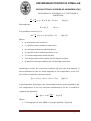
RESUMEN DEL PROYECTO
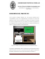
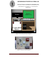
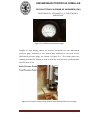
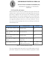
Con la ayuda de Siemens Industry, Inc., este proyecto apuesta por la
sostenibilidad a través de la implementación de sistemas de control. Una
plataforma móvil ha sido construida con el objetivo de contener un sistema
de control de calefacción de aire y una interfaz que muestre los parámetros
de configuración del controlador implementado y la respuesta del mismo. La
Figura 1.1 muestra el diseño de dicha plataforma.
Figura 1.1: Diseño de la plataforma móvil con el sistema de control.
Un pequeño compartimento dentro del dispositivo móvil funcionará como la
planta del sistema, en la cual el controlador deberá de regular la temperatura
del mismo. El sistema de control de aire introducirá aire caliente o a
Resumen.
Página 1
UNIVERSIDAD PONTIFICIA COMILLAS
ESCUELA TÉCNICA SUPERIOR DE INGENIERÍA (ICAI)
INGENIERO EN AUTOMÁTICA Y ELECTRÓNICA
INDUSTRIAL
temperatura ambiente para calentar o enfriar el compartimento y así
alcanzar la temperatura deseada en régimen permanente. El actuador del
sistema de control está formado por un ventilador y una resistencia eléctrica
cuyo voltaje es regulado por un controlador PID a través de modulación por
ancho de pulso (PWM).
Empleando el sistema de control construido y desarrollado, se han diseñado
dos guías de laboratorio que serán aplicadas por futuros estudiantes en los
laboratorios de termodinámica y de controles de la Universidad de San Diego,
donde este proyecto ha sido desarrollado.
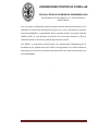
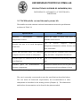
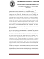
Gracias al diseño de una interfaz y la implementación de controles en
LabVIEW es posible la obtención de datos en tiempo real y realizar un
análisis termodinámico de
la eficiencia del sistema en las dos
configuraciones diseñadas (con y sin recalentamiento). En la práctica de
controles diseñada se podrá variar los parámetros del controlador para ver
su efecto en el sistema y comparar los resultados con el modelo no lineal que
se ha implementado en Matlab. Un ejemplo se muestra en la Figura 1.2
Comparison real system(LabVIEW)-simulation(Matlab)
Temperature (⁰C)
30,5
Simulation
(Matlab)
30
29,5
Real
system
(LabVIEW)
29
28,5
28
27,5
0
50
100
150
200
Time(sec.)
Figura 1.2 Comparación entre la respuesta del modelo real y simulación.
Resumen.
Página 2
UNIVERSIDAD PONTIFICIA COMILLAS
ESCUELA TÉCNICA SUPERIOR DE INGENIERÍA (ICAI)
INGENIERO EN AUTOMÁTICA Y ELECTRÓNICA
INDUSTRIAL
Por otro lado, el dispositivo móvil contiene además una demostración de los
sistemas de control de Siemens (Ver Figura 1.1) con la intención de mostrar
sus funcionalidades y capacidades. Dicho sistema incluye su propia Interfaz
Gráfica (GUI), la cual muestra al usuario de una forma intuitiva y fácil la
información de los sensores y demás aparatos de control.
Por último, el dispositivo móvil puede ser transportado fácilmente por la
totalidad de las instalaciones del edificio de ingeniería de la Universidad de
San Diego con el fin de ser una herramienta útil en las áreas relacionadas con
la sostenibilidad.
.
Resumen.
Página 3
UNIVERSIDAD PONTIFICIA COMILLAS
ESCUELA TÉCNICA SUPERIOR DE INGENIERÍA (ICAI)
INGENIERO EN AUTOMÁTICA Y ELECTRÓNICA
INDUSTRIAL
ABSTRACT
With the assistance of Siemens Industry, Inc., the TOCOM Lab demonstrates
energy sustainability through the implementation of control systems and
associated devices in a lab environment. A mobile lab unit was constructed
to contain an onboard air control system and display a configuration of
control system devices and instruments. The mobile lab unit is shown in
Figure 1.1.
Figure 1.1 Mobile lab unit design.
An enclosed space within the unit serves as a model environment in which a
control system will regulate the air temperature. A computer actuated air
control system introduces heated or outside air to heat or cool the space to
achieve a desired, steady-state temperature. The heating actuator comprises
Abstract.
Page 1
UNIVERSIDAD PONTIFICIA COMILLAS
ESCUELA TÉCNICA SUPERIOR DE INGENIERÍA (ICAI)
INGENIERO EN AUTOMÁTICA Y ELECTRÓNICA
INDUSTRIAL
a fan and a coil whose voltage is regulated by a PID controller through Pulse
Width Modulation (PWM).
Using the air control system, both a thermal systems and control systems lab
exercise was created with the aim to be applied by future students in
thermodynamics and controls labs in the University of San Diego, where the
project has been developed.
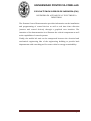
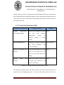
Real time data collection using LabVIEW allows for the analysis of the
thermal efficiency of the system with and without a reheat configuration.
The parameters of the control system can also be varied using LabVIEW to
provide an instructive exercise in the design of control systems. Furthermore,
the results gathered in the real system could be compared with the
simulation responses obtained when running the non linear model
implemented in Matlab. An example is shown in Figure 1.2.
Comparison real system(LabVIEW)-simulation(Matlab)
Temperature (⁰C)
30,5
Simulation
(Matlab)
30
29,5
Real
system
(LabVIEW)
29
28,5
28
27,5
0
50
100
150
200
Time(sec.)
Figure 1.2: Comparison between real system and simulation responses.
Abstract.
Page 2
UNIVERSIDAD PONTIFICIA COMILLAS
ESCUELA TÉCNICA SUPERIOR DE INGENIERÍA (ICAI)
INGENIERO EN AUTOMÁTICA Y ELECTRÓNICA
INDUSTRIAL
The Siemens Control Demonstration provides information on the installation
and programming of control devices as well as real time data collection
(sensors and control devices) through a graphical user interface. The
intention of the demonstration is to illustrate the critical components as well
as the capabilities of control systems.
Finally, the mobile lab unit can be transported between the electrical and
mechanical engineering labs of the engineering building to provide both
departments with a teaching tool for areas critical to energy sustainability.
Abstract.
Page 3
TOCOM LAB: Design of a controlled HVAV
system to implement in thermodynamic
and controls laboratories.
University of San Diego
2010-2011
Department of Engineering
Final Design Report
May 05, 2011
Report
Table of Contents
Part I:Report ................................................................. ¡Error! Marcador no definido.
Chapter 1 Introduction .................................................... ¡Error! Marcador no definido.
1.1Context ................................................................... ¡Error! Marcador no definido.
1.2Problem definition ................................................................................................ 3
1.2.1
Customer requirements ........................................................................... 3
1.2.2
Assumptions ............................................................................................ 5
1.2.3
Constraints ............................................................................................... 5
Chapter 2 Design specifications .................................................................................... 6
2.1 Design overview ................................................................................................... 6
2.2 Functional specifications ...................................................................................... 7
2.3 Physical specifications .......................................................................................... 8
Chapter 3 : Design analysis and results ....................................................................... 10
3.1 TOCOM mobile cart and thermal systems lab .................................................... 14
3.2 HVAC installation ............................................................................................... 16
3.3 Controls demonstration ..................................................................................... 20
3.4 Controller and sensors ....................................................................................... 33
3.5 Guide User Interface (GUI) ................................................................................. 39
Chapter 4: Implementation ........................................................................................ 44
4.1 Construction ...................................................................................................... 44
4.2 Testing ............................................................................................................... 51
4.2.1 TOCOM mobile cart ..................................................................................... 51
4.2.2 HVAC ........................................................................................................... 52
4.2.3 Controls ....................................................................................................... 55
4.2.4 Control systems lab ..................................................................................... 56
4.2.5 Thermal systems lab .................................................................................... 60
4.2.6 Controller and sensors ................................................................................. 63
Report
4.2.7 Guide User Interface (GUI)........................................................................... 66
References .................................................................................................................. 67
Part II: Budget .........................................................................................................68
Budget ..................................................................................................................... 69
Part III: Appendix ...................................................................................................72
Appendix A:Controller/ sensors and GUI interface ................................................. 73
A.1
Controller and sensors appendix................................................................ 73
A.2
GUI Appendix............................................................................................. 76
Appendix B: Thermal systems lab ........................................................................... 82
Appendix C: Controls lab ......................................................................................... 98
C.1
User’s manual ............................................................................................ 98
C.2
Programs ................................................................................................... 99
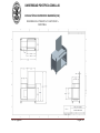
Appendix D: Plans ................................................................................................. 105
D.1
Cart assembly dimensioned ..................................................................... 106
D.2
HVAC installation ..................................................................................... 107
List of Figures
Figure 3.1 Block diagram for air control system ............. 1¡Error! Marcador no definido.
Figure 3.2 Block diagram for Siemens display .............................................................. 12
Figure 3.3 Overall system layout diagram .................................................................... 13
Figure 3.4 Picture of actual display .............................................................................. 13
Figure 3.5 Valve and end cap locations ........................................................................ 17
Figure 3.6 HVAC system layout .................................................................................... 19
Figure 3.7 DAQ interface diagram................................................................................ 20
Report
Figure 3.8 PWM ........................................................................................................... 22
Figure 3.9 PCB board ................................................................................................... 23
Figure 3.10 DAQ connections ...................................................................................... 24
Figure 3.11 Flowchart of the overall process ............................................................... 25
Figure 3.12 Simulink schematic model ......................................................................... 27
Figure 3.13 PWM LabVIEW interface ........................................................................... 31
Figure 3.14 LabVIEW programming ............................................................................. 32
Figure 3.15 PXC module .............................................................................................. 35
Figure 3.16 Siemens room temperature sensor and duct temperature sensor ............ 37
Figure 3.17 Air quality sensor ...................................................................................... 37
Figure 3.18 Relative humidity/temperature sensor ..................................................... 38
Figure 3.19 Variable Air Volume box and Actuating Terminal Equipment
Controller .................................................................................................................... 38
Figure 3.20 Back and Home buttons ............................................................................ 42
Figure 3.21 Created points menu ................................................................................ 43
Figure 4.1 CAD rendering of the TOCOM mobile lab .................................................... 44
Figure 4.2 Photograph of TOCOM mobile lab .............................................................. 45
Figure 4.3 Photograph of TOCOM mobile lab featuring Siemens display ..................... 46
Figure 4.4 HVAC system construction: ducts ................................................................ 47
Figure 4.5 Heating Coil enclosure ................................................................................ 47
Figure 4.6 System in standard flow configuration ........................................................ 48
Figure 4.7 System in reheating configuration .............................................................. 49
Figure 4.8 Differential pressure gage ........................................................................... 50
Figure 4.9 Probes connected to system and differential pressure gage ....................... 50
Figure 4.10 Comparison between real system and simulation responses .................... 59
Appendix ..................................................................................................................... 72
Figure 1.1 Fire Pull switch program flowchart .............................................................. 74
Figure 1.2 Occupancy switch program flowchart ......................................................... 76
Figure 1.3 GUI homepage ............................................................................................ 76
Report
Figure 1.4 First page .................................................................................................... 77
Figure 1.5 Temperature sensors page.......................................................................... 77
Figure 1.6 Duct temperature sensor page.................................................................... 78
Figure 1.7 Humidity/temperature readings ................................................................. 78
Figure 1.8 CO2 sensors page ........................................................................................ 79
Figure 1.9 Beginning page ........................................................................................... 79
Figure 1.10 Design page 2............................................................................................ 80
Figure 1.11 Design page 3............................................................................................ 80
Figure 1.12 Alarm page................................................................................................ 82
List of Tables
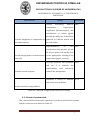
Table 3.1 Design description for mobile cart with enclosed environment .................... 14
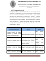
Table 3.2 design description for thermal systems lab .................................................. 15
Table 3.3 HVAC specifications and design .................................................................... 17
Table 3.4 Discrete periods ........................................................................................... 30
Table 3.5 LabVIEW specifications ................................................................................ 33
Table 3.6 Controls lab specifications ............................................................................ 33
Table 3.7 Design specifications .................................................................................... 34
Table 3.8 Specifications and deliverables for GUI ........................................................ 40
Table 4.1 Testing methods and results for mobile cart ................................................ 51
Table 4.2 HVAC testing ................................................................................................ 53
Table 4.3 Differential pressures and corresponding flow rates .................................... 55
Table 4.4 LabVIEW design specifications and testing ................................................... 56
Table 4.5 Matlab specifications and testing ................................................................. 57
Report
Table 4.6 Requirements testing for thermal system lab ............................................... 60
Table 4.7 Efficiency of the air temperature control system .......................................... 62
Table 4.8 Controller and sensor testing ....................................................................... 63
Table 4.9 Testing procedure and results for GUI .......................................................... 65
Budget ........................................................................................................................ 68
Table 1.1 Siemens display parts list ............................................................................. 69
Table 1.2 Parts list for HVAC components.................................................................... 70
Appendix ..................................................................................................................... 72
Table 1.1 Description of inputs and outputs ................................................................ 73
Report
PART I
REPORT
Report
UNIVERSIDAD PONTIFICIA COMILLAS
ESCUELA TÉCNICA SUPERIOR DE INGENIERÍA (ICAI)
INGENIERO EN AUTOMÁTICA Y ELECTRÓNICA
INDUSTRIAL
Chapter 1
Introduction
1.1
Context
In an effort to encourage continued focus on energy management and
sustainability the TOCOM group built a mobile lab unit which demonstrates
efficiency
and
energy
management
implementation of control systems.
building
systems
through
the
Working with a leader in energy
management, Siemens Industry Inc., the multidisciplinary team had the
opportunity to learn how modern building technologies can be used to
increase sustainability in operations, and used this knowledge to develop the
TOCOM Mobile Lab. The project was divided into two sections: Design and
construction of an air control system for a small environment and a
demonstration of the Siemens control devices. The air temperature control
system regulates the air temperature within an enclosed environment
through the use of a miniature heater and fan actuated through LabVIEW.
The Siemens control demonstration uses control devices and hardware to
show how to program and install real size sensors and display these readings
on a Graphical User Interface (GUI).
The two different sections will place their respective parts together on the
cart and share a computer that will have Insight and LabVIEW installed on it.
Part I. Report
Página 1
UNIVERSIDAD PONTIFICIA COMILLAS
ESCUELA TÉCNICA SUPERIOR DE INGENIERÍA (ICAI)
INGENIERO EN AUTOMÁTICA Y ELECTRÓNICA
INDUSTRIAL
Both groups must be aware of the size of each other’s components and to
ensure that the display is not only functional but easily accessible.
Air Control System:
An enclosed environment was constructed aboard the cart to contain the air
to be conditioned by the control system. The control system and heating,
ventilation, and air conditioning (HVAC) system integrated with the enclosed
environment will enable the TOCOM mobile lab to be used for both thermal
systems and control systems laboratory exercises. The thermal systems
laboratory focuses on comparing the system efficiency when air is directly
taken from the outside environment or re-circulated within the system. The
efficiency can be analyzed through the calculation of heat and power input
values based on real time measurements. The control systems lab focuses on
the design of control systems using the physical actuators and sensor devices
aboard the cart.
Siemens Control Demonstration:
The Siemens control demonstration portion of this project was developed
with the help of Siemens Industry Inc.. The Siemens display will feature a
Programmable Controller (PXC) that is the main processor for all information
generated in the Siemens lab.
On the cart, a group of sensors for
Temperature, Humidity, and carbon dioxide (CO2) are to be placed on a
display panel so that they can be easily seen. On the display panel there is
also a Fire Alarm Pull Switch, Fire Strobe Light, and a Terminal Equipment
Controller (TEC). Placed below this panel is a Variable Air Volume (VAV) box
with an attached Actuating Terminal Equipment Controller (ATEC) that will
turn the damper in the VAV box along with measuring pressure drops. This
information is sent to the PXC through the Floor Level Network (FLN) and
Part I. Report
Página 2
UNIVERSIDAD PONTIFICIA COMILLAS
ESCUELA TÉCNICA SUPERIOR DE INGENIERÍA (ICAI)
INGENIERO EN AUTOMÁTICA Y ELECTRÓNICA
INDUSTRIAL
the readings from the other sensors and buttons are wired directly into the
PXC.
All of the previously stated information is to be displayed on the GUI. The
GUI is placed on the main computer also located on the cart. The GUI is to be
easily accessible and user friendly while also allowing a user to learn about
the system’s design.
1.2 Problem definition.
The problem that this project is attempting to solve is to successfully
implement a mobile lab with an onboard controlled environment to
propagate knowledge critical to energy management and sustainability. The
mobile lab must facilitate its own transportation within the confines of the
engineering labs in Loma Hall. The lab, which caters to more advanced users
in the form of control systems and thermal systems labs, must also be able to
serve as teaching tool for the basics of control systems and associated devices
for any person who interfaces with the lab. University of San Diego (USD) is
increasing
its
sustainability
campus
wide;
demonstrating
energy
sustainability with an engineering controls lab will serve as yet another
example of its efforts to increase sustainability.
1.2.1 Customer Requirements
The customers for this project, USD students, faculty, and staff, require a
mobile lab that has the following characteristics:
1. Measurements
of
the
surrounding
environment,
including
temperature, humidity, and CO2 content of the air displayed on a GUI
running on an onboard computer
Part I. Report
Página 3
UNIVERSIDAD PONTIFICIA COMILLAS
ESCUELA TÉCNICA SUPERIOR DE INGENIERÍA (ICAI)
INGENIERO EN AUTOMÁTICA Y ELECTRÓNICA
INDUSTRIAL
2. All components need to be visible and clearly identified to users,
interacting with the unit
3. Safe mobile lab unit for future use by USD students, faculty, and staff
4. Laboratory exercises which can be performed in both thermal science
and control systems engineering using the mobile lab
5. An easily navigable GUI conveying information concerning control
system devices
Physical Requirements
The mobile cart unit will present unobstructed visual of air handling
equipment, control devices, and other sensors. All components need to be
physically supported as well.
Since the mobile cart will be used as a teaching tool in different labs, it must
be mobile and able to fit in engineering labs and the elevator.
An onboard computer must be supported physically and electronically
Functional Requirements
TOCOM’s mobile cart must fulfill the following requirements:

GUI allows user to interface with control system devices.

Confined space must be able to maintain a prescribed temperature at
steady state.

Construction and implementation costs less than projected budget.

Readings for temperature, CO2, and humidity displayed for public
access.

Entire control system can be displayed to users.
Part I. Report
Página 4
UNIVERSIDAD PONTIFICIA COMILLAS
ESCUELA TÉCNICA SUPERIOR DE INGENIERÍA (ICAI)
INGENIERO EN AUTOMÁTICA Y ELECTRÓNICA
INDUSTRIAL

The GUI, LabVIEW, and both the thermal and control systems lab
exercises need to be stored on the computer that can be used by a
person standing up or seated on an elevated lab chair
1.2.2 Assumptions
The design has been constructed based on the following assumptions:

The TOCOM Mobile Lab will be used within in the engineering labs.

Siemens will provide the team with the suitable components in
accordance with a budget.

The lab cart will have access to a power supply whenever it is to be
used
1.2.3 Constraints
On the one hand, laboratory must conform to safety protocols for electrical
and mechanical safety, so users will be protected from moving parts, sources
of heat, and electrically isolated from dangerous components such as wires
or transformers.
On the other hand, laboratory and components must be contained on the
mobile cart to make it easier to use and move.
Finally, components concerned with the Siemens Control Demonstration
must be obtained from Siemens and their software Insight must be used as
well.
Part I. Report
Página 5
UNIVERSIDAD PONTIFICIA COMILLAS
ESCUELA TÉCNICA SUPERIOR DE INGENIERÍA (ICAI)
INGENIERO EN AUTOMÁTICA Y ELECTRÓNICA
INDUSTRIAL
Chapter 2
Design specifications
Before
going
into
details
about
contruction,
programming
and
implementation, this chapter has the aim to explain the specifications that
the different subsystems have to fulfill. Setting the specifications is really
important to understand the different subsystems involved in the project,
meet the requirements and come up with a suitable design.
2.1 Design overview
As it has been mentioned before, the project is basically composed by two
sections whose overall design is going to be described next.
Air Control System
The footprint of the constructed laboratory is 4 feet in length and 25 inches
in width to facilitate transportation throughout the enginnering building.
The most important goal of this lab design is that it be able to maintain a
controlled environment while at the same time being able to demonstrate the
energy efficiency capable through the use of control systems. The control
system maintains the environment by intermittently hot air or pumping fresh
air to achieve a steady-state temperature.
Part I. Report
Página 6
UNIVERSIDAD PONTIFICIA COMILLAS
ESCUELA TÉCNICA SUPERIOR DE INGENIERÍA (ICAI)
INGENIERO EN AUTOMÁTICA Y ELECTRÓNICA
INDUSTRIAL
Siemens Control Demonstration
To convey the basics of control systems and their associated devices, the lab
is be outfitted with a series of sensors for temperature, humidity, and CO2.
The lab is also equipped with a VAV box which demonstrates how the
controlled environments in building systems are regulated.
2.2 Functional specifications
Primary functions of the project are related to the user interaction with
laboratory exercises and the Siemens Control Demonstration. Users must be
able to activate all components via the onboard computer or switch related to
the demonstration. Descriptions of the projects functional specifications are
explained in more detail below.
A. Maintain Temperature

Temperature sensor reads actual temperature within a range
supporting the lab exercises.

A fan and heating coil add a heated volume flow rate to the enclosed
environment.

The virtual control system, run in LabVIEW, interfaces with the
physical system via a DAQ (Data AcQuisition device).
B. Provide Exercise in Thermal Efficiency Analysis

The thermal systems lab provides an opportunity to analyze and
compare efficiency of different thermal systems.

Onboard data collection facilitating the calculation of efficiency.

Variable system configuration allowing for comparison of similar
systems with and without recirculation of conditioned air.
Part I. Report
Página 7
UNIVERSIDAD PONTIFICIA COMILLAS
ESCUELA TÉCNICA SUPERIOR DE INGENIERÍA (ICAI)
INGENIERO EN AUTOMÁTICA Y ELECTRÓNICA
INDUSTRIAL
C. Provide Exercise in Control Systems Engineering

The control system of the enclosed environment can be changed in
accordance with user input.

The lab shows how variation Proportional-Integral-Derivative (PID)
controller parameters will change how the system response to a
desired input.

The lab will be equipped to show how a non-linear system can be
converted to a linear system and the results will be displayed.
D. Display Values of Sensors

The sensors on the lab provide real time measurements to the GUI.

The control devices provide responses to user inputs to the switches
installed on the cart.

The controller is programmed to run specific routines if specific
inputs are detected.
2.3 Physical specifications
The TOCOM Lab was required to be mobile, allowing for the transportation of
the cart between different labs in engineering’s building implying it would be
able to fit through doors and on the elevator. The TOCOM Lab was built
aboard a cart which has a footprint of roughly 4ft by 2ft and a maximum
height of 64 inches. The cart is mounted on 4 swivel wheels which facilitate
positioning within the labs. The TOCOM Mobile Cart supports the onboard
subsystems by providing each with adequate space while allowing for user
interaction with the onboard computer system.
Part I. Report
Página 8
UNIVERSIDAD PONTIFICIA COMILLAS
ESCUELA TÉCNICA SUPERIOR DE INGENIERÍA (ICAI)
INGENIERO EN AUTOMÁTICA Y ELECTRÓNICA
INDUSTRIAL
The HVAC system was designed to house and insulate a heat source and fan.
The circuit is constructed of both Acrylonitrile Butadiene Styrene (ABS) and
PolyVinyl Chloride (PVC) plastic tubing.
The inlet and exhaust to the
enclosed environment are both 1 inch in diameter. The heater and fan
housings are each 3 inches in diameter with variable diameter steps
interfacing the two different tube sizes. The HVAC system safely provides the
heated air necessary for the lab exercises.
Part I. Report
Página 9
UNIVERSIDAD PONTIFICIA COMILLAS
ESCUELA TÉCNICA SUPERIOR DE INGENIERÍA (ICAI)
INGENIERO EN AUTOMÁTICA Y ELECTRÓNICA
INDUSTRIAL
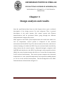
Chapter 3
Design analysis and results
Once the specifications have been set, this chapter tries to give a technical
description of the design process for each subsytem. First, a general
description of the main systems (Air control system and Siemens
demonstration) will be presented before going through the different
subsystems that comprise the project.
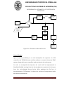
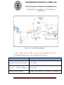
With regards to the HVAC system implemented, the small scale model of a
real air temperature control system is composed of the enclosed
environment and the HVAC loop. The valve actuators, fan motor, and electric
resistive heating coil within the HVAC loop are activated and controlled by
relays thrown by the control system. Operated through a computer with
LabVIEW and interfaced to the HVAC loop through a data acquisition device
(DAQ), the control system actuates the devices to control the air temperature
in the enclosed environment. The control system compares the measured
temperature to a user specified temperature and responds by adding heated
or cool air to the enclosed environment. The block diagram for the HVAC
Demonstration is shown below in Figure 3.1.
Part I. Report
Página 10
UNIVERSIDAD PONTIFICIA COMILLAS
ESCUELA TÉCNICA SUPERIOR DE INGENIERÍA (ICAI)
INGENIERO EN AUTOMÁTICA Y ELECTRÓNICA
INDUSTRIAL
Figure 3.1: Block diagram for air control system
The Siemens display is composed of a PXC Controller that is connected to a
group of sensors that send their respective results back to the controller for
analysis. In addition to the sensors a Fire Alarm Pull Switch is connected to
the controller which turns a Fire Strobe Light on when pulled. All of these
values along with an explanation for the system’s design are placed in a GUI
Part I. Report
Página 11
UNIVERSIDAD PONTIFICIA COMILLAS
ESCUELA TÉCNICA SUPERIOR DE INGENIERÍA (ICAI)
INGENIERO EN AUTOMÁTICA Y ELECTRÓNICA
INDUSTRIAL
which is easily accessible and readable to the user. The block diagram for the
Siemens display is shown in Figure 3.2.
Figure 3.2 Block diagram for siemes display
A system layout diagram is shown in Figures 3.3 and 3.4 for the overall
system.
Part I. Report
Página 12
UNIVERSIDAD PONTIFICIA COMILLAS
ESCUELA TÉCNICA SUPERIOR DE INGENIERÍA (ICAI)
INGENIERO EN AUTOMÁTICA Y ELECTRÓNICA
INDUSTRIAL
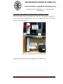
Figure 3.3 Overall system layout diagram.
Figure 3.4 Picture of actual display
Part I. Report
Página 13
UNIVERSIDAD PONTIFICIA COMILLAS
ESCUELA TÉCNICA SUPERIOR DE INGENIERÍA (ICAI)
INGENIERO EN AUTOMÁTICA Y ELECTRÓNICA
INDUSTRIAL
3.1 TOCOM mobile cart and thermal systems lab
The mobile cart with onboard enclosed environment meets the specifications
as shown in Table 3.1.
Specifications
Enclosed
environment
Design
enabling Sealed box made of wood with door to
temperature control
facilitate sensor access
Portable lab unit to be used throughout
Loma Hall
Cart
on
wheels
supports
onboard
subsystems, dimensions within elevator and
door constraints
Stores and provides space for onboard Space provided for computer tower, monitor,
computer used for control of subsystems
DAQ, and other components aboard cart
Provides space for onboard HVAC and air- HVAC loop installed and functioning onboard
recycling loop
Provides
space
cart
for
Siemens components
demonstration
of Backboard constructed on cart for placement
of components and concealment of wires
Table 3.1 Design description for mobile cart with enclosed environment
The cart is currently constructed to meet the specifications described above.
The cart meets all functional requirements; the accommodation of other
subsystems is described in the testing section (Chapter 4). The dimensions
and further documentation can be found in the plans attached.
Part I. Report
Página 14
UNIVERSIDAD PONTIFICIA COMILLAS
ESCUELA TÉCNICA SUPERIOR DE INGENIERÍA (ICAI)
INGENIERO EN AUTOMÁTICA Y ELECTRÓNICA
INDUSTRIAL
By following the lab procedure (found in Appendix, Chapter 2), students can
investigate and compare the efficiency of an air temperature control system
to a similar system utilizing an air recirculation loop. The thermal systems
lab meets the required specifications, as seen in Table 3.2.
Specifications
Thermal
systems
lab
Design
will
enable
students to compare power savings
due to recycling loop.
Lab
handout
directs
students
to
measure and compare efficiency for
HVAC operation with and without the
recycling loop.
4 Thermocouple [T1] placed within the
Temperature readings before and after enclosed environment (output) and
addition of heat.
another [T2] within the HVAC duct
upstream of the fan.
Ability to measure power provided to
fan and heating element.
Voltage supplied to each device know,
Power is collected real-time using
LabVIEW.
User observes differential pressure
reading
of
airflow,
from
this
Ability to measure volume airflow measurement mass flow rate through
through the system.
system
can
be
calculated
using
provided equations and background on
theory.
Table 3.2 Design description for thermal systems lab
While the control system regulates the HVAC system to achieve a steadystate temperature, the thermal systems lab exercise can be completed. The
Part I. Report
Página 15
UNIVERSIDAD PONTIFICIA COMILLAS
ESCUELA TÉCNICA SUPERIOR DE INGENIERÍA (ICAI)
INGENIERO EN AUTOMÁTICA Y ELECTRÓNICA
INDUSTRIAL
lab handout describes the procedures for the collection of data, conversion to
SI unit system, and calculation of desired values. The temperature set points
of the lab will not exceed 33 ⁰C for both system configurations. These values
were chosen based on time to reach steady-state.
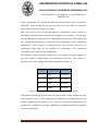
3.2 HVAC installation
This system is used to ventilate an enclosed environment and manipulate the
temperature of the air. The system utilizes a fan that pushes air over a
heating coil to manipulate the temperature of the enclosed space. The team
designed a HVAC system that would meet the specifications and the
corresponding design requirements as shown in Table 3.3.
Specification
Provide a constant, measurable
flow rate 14.7 CFM
Ability to heat air from room
temperature to 37.5 ⁰C
Design
Fan controlled by LabVIEW, verified by
taking
pressure
readings
from
a
differential pressure sensor
Controlled heating element (obtained
from hair dryer designed not to exceed
60 ⁰C)
Heating element contained inside ABS
System withstands temperature piping which is rated up to 76.7 ⁰C which
of heating element
exceeds
the
element’s
maximum
temperature
System fits inside cart.
Part I. Report
System designed to fit inside and on cart
25” x 50” x 32”
Página 16
UNIVERSIDAD PONTIFICIA COMILLAS
ESCUELA TÉCNICA SUPERIOR DE INGENIERÍA (ICAI)
INGENIERO EN AUTOMÁTICA Y ELECTRÓNICA
INDUSTRIAL
System must be able to run both Piping, valve, and cap are arranged in
standard
flow
and
re-circulation such a way that the system can exhaust
the air or re-circulate the air.
Table 3.3 HVAC Specifications and Design
The layout of the system was designed to fit within the dimensions of the
cart. The scale drawings of the system can be found in plans attached. The
system layout found in Figure 3.3 is to scale and also shows HVAC system
installed on the cart. When the system is set for a recirculation process, the
exhaust valve is closed and the end cap is removed. The exhaust valve is
placed such that when it is closed the air is redirected back through the
system when the cap is removed. A digital model from ProE of the system
denoting the locations of the valve and end cap can be found in Figure 3.5.
Figure 3.5 Valve and End Cap Locations
Part I. Report
Página 17
UNIVERSIDAD PONTIFICIA COMILLAS
ESCUELA TÉCNICA SUPERIOR DE INGENIERÍA (ICAI)
INGENIERO EN AUTOMÁTICA Y ELECTRÓNICA
INDUSTRIAL
The HVAC system’s piping, valve, and cap were purchased, assembled, and
installed together. The fan and heating coil have also been acquired and
installed into the system. The fan and heater are mounted into black ABS
housing sections using an adhesive pipe insulation which is rated for
temperatures up to 76.7 ⁰C. ABS was chosen as the housing for the heater
because of its high heat tolerance and availability. PVC was used for the
remaining sections of the systems piping because of ease to assemble and
available sizing. The entire HVAC system has been mounted on the cart and
connected to the contained space. The inlet and exhaust pipes extend into
the contained space to facilitate the circulation of air through the space.
In order to properly heat and ventilate this system a constant flow rate is
needed. The control system varies the heat applied to the flow in order to
manipulate the environment. The heating coil used in the system was taken
from a hair dryer. Initially the team decided to use a hair dryer’s heating
element because of its fast response time and small size. While taking the
hair dryer apart the team realized the small, inline fan contained with it was
an ideal fan for the HVAC system. The fan is almost three inches in diameter
and thus fits inside the three inch diameter ABS tubing. By testing the system
with the fan and heating coil installed and working the team was then able to
determine a proper flow rate. If the flow rate is too low the system will not
react quickly enough and heating coil may over heat. If the flow rate is too
high the air passing over the heating coil will not get hot enough to
adequately heat the enclosed environment. The team was able to find a
range of flow rates that worked for the system. (For more information on the
flow rate please see testing section, Chapter 4.)
A differential pressure gage has been installed into the enclosed
environment. Total and static pressure probes coming from the differential
pressure gage are installed into the HVAC system at the same location, shown
Part I. Report
Página 18
UNIVERSIDAD PONTIFICIA COMILLAS
ESCUELA TÉCNICA SUPERIOR DE INGENIERÍA (ICAI)
INGENIERO EN AUTOMÁTICA Y ELECTRÓNICA
INDUSTRIAL
in Figure 3.6, after the fan and heating coil housing. The total pressure probe
is installed parallel to the airflow using a metal rod to hold it straight. The
static pressure probe is installed perpendicular to the direction of airflow.
The differential pressure gage provides students with a differential pressure
reading in Inches Water Column. Students following the lab instructions will
use this value to calculate the flow rate in the system. (The process to
calculate flow rate from a pressure reading is shown in the lab instructions.)
Figure 3.6 HVAC System Layout
Thermocouples have been installed into the system as well.
The
thermocouples were used to test the ability of the heating coil to heat the air
as specified by the user through LabVIEW. Figure 3.6 also shows the location
of the inlet temperature thermocouple. This sensor is used to measure the
temperature of the air before it passes over the heating coil.
Another
thermocouple is placed inside of the control volume to measure the
temperature of the air after it has passed over the heating coil.
These
measurements provide feedback to the control system.
Part I. Report
Página 19
UNIVERSIDAD PONTIFICIA COMILLAS
ESCUELA TÉCNICA SUPERIOR DE INGENIERÍA (ICAI)
INGENIERO EN AUTOMÁTICA Y ELECTRÓNICA
INDUSTRIAL
3.3
Controls demonstration
The major goal of the controls subsystem is to serve as a practical tool in the
design of control systems, which are crucial in the majority of industrial
systems.
The main goals that the controls subsystem will allow the user to accomplish
are:

Analyze and observe the main features of the response in a control
system: stability, precision, speed, and overshoot.

Design of controllers through frequency response techniques starting
from stability, speed, and overshoot specifications.

Observe the differences between simulation and real systems.
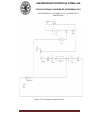
Some important tasks have to be accomplished in the design of the control
system, data acquisition, and components choice. The data acquisition
consists of gathering samples of the real world (analogical system) to
generate data that can be manipulated by a PC or another electronic system
(digital system). The device that transforms the signal used by the computer
is the DAQ (data acquisition device).This process can be shown in Figure 3.7.
Figure 3.7 DAQ Interface diagram
Part I. Report
Página 20
UNIVERSIDAD PONTIFICIA COMILLAS
ESCUELA TÉCNICA SUPERIOR DE INGENIERÍA (ICAI)
INGENIERO EN AUTOMÁTICA Y ELECTRÓNICA
INDUSTRIAL
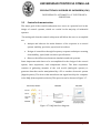
The three different parts that comprise the subsystem (input/output
components choice, DAQ selection/software, and control design) will be
explained in-depth:
DAQ selection and software
The DAQ that has been chosen for this project is the DAQ NI USB 6008, which
belongs to National Instruments and has the following features [4]:
 8 analog inputs (+/- 10 volts)
 analog outputs from 0 to 5 volts (12bits)
 12 digital input/outputs con logic values from 0 to 5 volts.
 Counter of 32 bits
This device is able to carry out multiple tasks simultaneously which means
that the USB 6008 can gather information and generate analog and digital
outputs at the same time. This capability is indispensable to develop a control
system.
Since the DAQ works better with software belonging to the same company
(National Instruments), LabVIEW is the most suitable tool to use. LabVIEW is
a graphic programming language for the design of data acquisition systems,
instrumentation, and controls. In addition, it is compatible with programs or
other applications like MATLAB. Thus, the controls design will be
implemented in MATLAB, but imported and run in LabVIEW.
Hardware components
The control systems that will be studied is a non-linear SISO system (single
input-single output) which means that one variable will be controlled
(temperature inside the enclosed environment) through one actuator
Part I. Report
Página 21
UNIVERSIDAD PONTIFICIA COMILLAS
ESCUELA TÉCNICA SUPERIOR DE INGENIERÍA (ICAI)
INGENIERO EN AUTOMÁTICA Y ELECTRÓNICA
INDUSTRIAL
(resistive coil). In this sense, the rest of components (fan) will be
independently activated from the control loop by the DAQ.
The temperature sensors chosen are 4 NI USB-TC01 thermocouples that will
be directly hooked up to the USB port on the computer. These thermocouples
will be placed inside the box so they will take an average temperature.
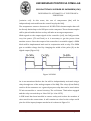
With regards to the output signal of the controller (coil), the DAQ provides
very few power (5V and 5mA) so it is necessary to get the power from
another source. Since the output of the controller is a variable signal, a PWM
block will be implemented and used in conjunction with a relay .The PWM
gets a variable voltage level by changing the width of the pulse (D) at the
digital output (Figure 3.8).
Figure 3.8 PWM
As it was mentioned before the fan will be independently activated using a
relay through one of the analog outputs of the DAQ. The relays (from Zetler)
used in all the actuators are a general purpose relay that can be used with a
5V microcontroller or control circuitry. The coil draws 72mA when engaged
and the relay can switch up to 2A at 30V (or 1A at 125V).
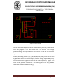
A PCB board has been installed to ensure safety and reduce the number of
wires used in the connections. It will contain two slots for the relays and 8
pins for all the inputs/outputs needed as it is shown in Figure 3.9.
Part I. Report
Página 22
UNIVERSIDAD PONTIFICIA COMILLAS
ESCUELA TÉCNICA SUPERIOR DE INGENIERÍA (ICAI)
INGENIERO EN AUTOMÁTICA Y ELECTRÓNICA
INDUSTRIAL
Figure 3.9 PCB board
The two relays will be powered by two transformers (24V each) connected in
series and plugged to the wall, so that 48V are obtained. This voltage
produces enough heating in the coil and velocity in the fan to reach the
requirements.
In short, the analog inputs 0,1,2,3 (AI0,AI1,AI2,AI3) and ground will be used
to gather data from the thermocouples; and the analog outputs (AO0/AO1)
serve as the control signals for the coil and fan respectively. Figure 3.10
shows all the possible connections in the analog part of the DAQ and the
connections that are used are in red [4].
Part I. Report
Página 23
UNIVERSIDAD PONTIFICIA COMILLAS
ESCUELA TÉCNICA SUPERIOR DE INGENIERÍA (ICAI)
INGENIERO EN AUTOMÁTICA Y ELECTRÓNICA
INDUSTRIAL
Figure 3.10 DAQ Connections
To make clear all the concepts developed below; Figure 3.11 depicts the flow
chart of the entire process.
Part I. Report
Página 24
UNIVERSIDAD PONTIFICIA COMILLAS
ESCUELA TÉCNICA SUPERIOR DE INGENIERÍA (ICAI)
INGENIERO EN AUTOMÁTICA Y ELECTRÓNICA
INDUSTRIAL
DAQ USB 6009
Digital output
To relays
DEACTIVATE
FAN
YES
Set temperature
Equal?
NO
NO
CONTROLLER
(PID,labview)
Temperature
Sensor Inside
box
(USB TC01)
PWM
(LabVIEW)
RELAY
(POWER THE
COIL)
DAQ USB 6009
(analog)
DAQ USB 6009
Digital output
To relays
ACTIVATE
FAN,POSITION
DAMPERS
Figure 3.11 Flowchart of Overall Process
Control design
Apart from the possibility to see and manipulate the response of a PID
controller, the TOCOM lab aims to allow students to research about the HVAC
system, design their own controllers, and test them in the real system.
In order to accomplish this objective the model will be implemented in
Simulink (Matlab) starting from the thermodynamics equations for the open
loop (no recirculating) shown below. After applying the fist law of
thermodynamics [3], Equation 3.1 shows the variation of temperature inside
the enclose environment.
Part I. Report
Página 25
UNIVERSIDAD PONTIFICIA COMILLAS
ESCUELA TÉCNICA SUPERIOR DE INGENIERÍA (ICAI)
INGENIERO EN AUTOMÁTICA Y ELECTRÓNICA
INDUSTRIAL
(Eq.3.1)
Knowing that:
It is possible to derive Eq. 3.2:
(Eq.3.2)
Where:





T: current temperature inside the box

Tair: temperature of the outside air (25 degrees Celsius)

Amount of heat provided by the coil through convection.
Assuming no losses, the convection equation [3] gives the total amount of
heat transmitted to the air, which depends on the temperature of the coil,
area of the coil and the convection factor.
(Eq 3.3)
A third equation, which gives the relationship between power applied to the
coil, temperature of the coil, and heat transmitted to the air, is needed to
complete the dynamics.
(Eq 3.4)
Where:

: Average power after PWM= u (voltage applied) x T(period)
Part I. Report
Página 26
UNIVERSIDAD PONTIFICIA COMILLAS
ESCUELA TÉCNICA SUPERIOR DE INGENIERÍA (ICAI)
INGENIERO EN AUTOMÁTICA Y ELECTRÓNICA
INDUSTRIAL

M: mass of the coil

C: specific heat constant of the coil
It is important to remember that the use of PWM in the actuator introduces
non-linearities, so this model brings the possibility to develop new
controllers by finding and setting the operating point and getting a linear
model. Once the linear model is obtained it is possible to study the frequency
response starting from the transfer function and design another controller
which will make the system obtain the different specifications.
The set point that has been chosen is 28
for the temperature inside the
box.
Using Eq 3.2, 3.3, and 3.4, final non-linear system’s schematic implemented in
Simulink is shown below in Figure 3.12.
Part I. Report
Página 27
UNIVERSIDAD PONTIFICIA COMILLAS
ESCUELA TÉCNICA SUPERIOR DE INGENIERÍA (ICAI)
INGENIERO EN AUTOMÁTICA Y ELECTRÓNICA
INDUSTRIAL
Figure 3.12: Simuling schematic model
Part I. Report
Página 28
UNIVERSIDAD PONTIFICIA COMILLAS
ESCUELA TÉCNICA SUPERIOR DE INGENIERÍA (ICAI)
INGENIERO EN AUTOMÁTICA Y ELECTRÓNICA
INDUSTRIAL
Dynamic’s initial parameters are calculated to run the simulation:

Voltage=60

Tair=

M_Air (mass of air in the box)= 0.15 Kg

Air flow (

Cv=
): Using the set point in Table 4.3, 14.75 CFM= 0.008 Kg/s.
Knowing that the coil utilized is made of Nicrom (density= 8400
), the
following values are obtained:

M_coil (mass of the coil): 30 gr.

C_coil(specific heat constant of the coil made of Nicrom):

A (Area of coil) = 62.83

Coil_resistance=10.25
Assuming turbulence air flow and forced convection, the convection factor
obtained is:

h=47
Thus,the non linear system model brings the possibility to come up with a
linear transfer function around the operating point.The procedure consists
on taking the output and input of the plant (Figure 3.12) in the operating
point and apply and iterative algorithm to get the value of the transfer
function parameters when the error approaches to zero. Since the plant
includes an integrator it is necessary to add a close-loop proportional
controller to the plant, so that the identification can be obtained without
unestabilities. In this case a proportional controller of K=0.2 has been applied
successfully. Files programmed in Matlab for identification are included in
the Appendix, Chapter 3.
Part I. Report
Página 29
UNIVERSIDAD PONTIFICIA COMILLAS
ESCUELA TÉCNICA SUPERIOR DE INGENIERÍA (ICAI)
INGENIERO EN AUTOMÁTICA Y ELECTRÓNICA
INDUSTRIAL
Finally, the linearization allows to design the final controller to be
implemented in the system.
Considerations in controller design
The implementation of both analog PID controller and PWM give rise to a
discrete controller which means that the period of the PWM is crucial when it
comes to design the controller. An unsuitable choice of the period can lead to
an unstable response.
To make clear the limitations of the design Table 3.4 shows the ratio between
the speed in open loop (controller design multiplied by the plant) and the
period of sampling (PWM)[1].
After designing the controller this ratio has to be checked so that it has to be
in the range of small. If the controller is not included or close to the range it
has to be redesigned or the PWM period changed.
Period
wTs
Big
Medium
2
0.5
Table 3.4: Discrete periods
Small
0.1
In this case, the period utilized should not be a problem since the constant
time of the process (temperature dynamics) is big enough to use a big range
of periods. A range from 1sec. to 10 sec is recommended.
Finally, a PID controller will be provided with the aim to be a reference for
future comparisons between controllers [2]. PWM parameters are also
included:

Kp=10

Ki=0.1

Kd=0.01

Precision=25

PWM period=5 sec.
Part I. Report
Página 30
UNIVERSIDAD PONTIFICIA COMILLAS
ESCUELA TÉCNICA SUPERIOR DE INGENIERÍA (ICAI)
INGENIERO EN AUTOMÁTICA Y ELECTRÓNICA
INDUSTRIAL

Amplitude=5
LabVIEW interface.
As mentioned before, the LabVIEW interface should include the controller in
charge of activating the actuator of the controlled system (coil) and the
fan.The standard controller implemented is a PID, which will be used in
conjunction with Pulse Width Modulation (PWM) to activate the relay of the
coil, so the analog output signal of the controller is converted into a digital
signal [5]. Users will be able to configurate PID and PWM parameters.
LabVIEW interface is shown in Figure 3.13. LabVIEW schematic including
controller and PWM is shown in Figure 3.14.
Figure 3.13: PWM LabVIEW interface
Part I. Report
Página 31
UNIVERSIDAD PONTIFICIA COMILLAS
ESCUELA TÉCNICA SUPERIOR DE INGENIERÍA (ICAI)
INGENIERO EN AUTOMÁTICA Y ELECTRÓNICA
INDUSTRIAL
Figure 3.14: LabVIEW programming.
In short, Table 3.5 and Table 3.6 show the specifications and the
corresponding design that the controls subsystems must meet.
Specifications
Accurate
integration
Design
of 4 USB thermocouples as inputs and 2 digital outputs
components in the control system
(coil and fan).
Provide enough power to the
actuators
( fan, coil, dampers)
Accurate control response
Part I. Report
Use of relays
Provide a PID controller as a reference to comparece it
Página 32
UNIVERSIDAD PONTIFICIA COMILLAS
ESCUELA TÉCNICA SUPERIOR DE INGENIERÍA (ICAI)
INGENIERO EN AUTOMÁTICA Y ELECTRÓNICA
INDUSTRIAL
with other controllers.
Interface that allows to introduce the controller
parameters,
Intuitive interface using LabView
PWM
parameters,
and
the
desired
temperature easily.
Table 3.5: LabVIEW specifications
Specifications
Design
Provide a tool that identifies the File that calculates the parameters of the transfers
transfer function of the system.
Provide
a
tool
that
gives
function’s plant by using an iterative algorithm.
the
parameters and expression of a
certain PID controller for specific File that provides the parameters of the PID controller
requirements.
given the different specifications.
Bring the possibility to export the
results from Matlab to Labview and
see
the
differences
simulation and real system.
between
Intruduce a file that exports data to an excell file.
Table 3.6: Controls lab specifications
Part I. Report
Página 33
UNIVERSIDAD PONTIFICIA COMILLAS
ESCUELA TÉCNICA SUPERIOR DE INGENIERÍA (ICAI)
INGENIERO EN AUTOMÁTICA Y ELECTRÓNICA
INDUSTRIAL
3.4
Controller and sensors
The controller and sensor subsystem includes the installation, wiring, and
programming of the controller and sensors involved in the Siemens Display.
Table 3.7 shows the design specifications for the subsystem.
TOCOM Lab Siemens Display
Specifications
Design
Controller detects when digital input is
Fire pull switch that triggers alarm
triggered by pull switch. Controller
enables light and alarm.
Actuate the sample damper
Wall switch that indicates occupancy
Controller
rotates
the
damper
on
command to simulate airflow.
When user triggers the switch, system
responds to occupancy and enables fan
Implement temperature, humidity, and All components were placed on a 26.5” x
CO2 sensors on a mobile unit
24” backboard on the cart
Table 3.7 Design specifications.
The controller being used is the PXC Modular Series (PXC100-PE) shown in
Figure 3.15. This controller has the capability to be expanded using Terminal
Blocks, or input/output (I/O) modules, with support for up to 500 I/O points.
These points are for connecting sensors, actuators, switches and buttons.
The Terminal Blocks can be selected and added on to the controller based on
the type of job needing to be accomplished.
Each block has different
capabilities [6],[7].
Part I. Report
Página 34
UNIVERSIDAD PONTIFICIA COMILLAS
ESCUELA TÉCNICA SUPERIOR DE INGENIERÍA (ICAI)
INGENIERO EN AUTOMÁTICA Y ELECTRÓNICA
INDUSTRIAL
Figure 3.15 PXC Module with Terminal Expansion Blocks.
The first block, shown in Figure 3.15 (block A), is the power supply
(TXS1.12F4) for the I/O Modules. It has a 24 VAC (volts of alternating
current) input used to power it and the expansion blocks. The power supply
also converts the 24 VAC into 24 volts direct current (VDC) to provide power
for some of the sensors and other components that require DC.
The next module, in Figure 3.15 block B, is a 16 point digital input (DI) block
(TXM1.16D). Refer to Appendix (Table 1.1, Chapter 1) for input and output
descriptions. This module monitors normally open or normally closed dry
contacts (voltage free) for up to 16 inputs. The third block, in the same
Figure 3.15 block C, is a digital output (DO) module with manual override
(TXM1.6R-M). This block provides six normally open or normally closed
voltage free contacts with a maximum rated voltage of up to 250 VAC at 4
amperes (A). The override button allows for each point to be controlled
manually on the Terminal Block itself. It has green light emitting diodes
Part I. Report
Página 35
UNIVERSIDAD PONTIFICIA COMILLAS
ESCUELA TÉCNICA SUPERIOR DE INGENIERÍA (ICAI)
INGENIERO EN AUTOMÁTICA Y ELECTRÓNICA
INDUSTRIAL
(LEDs) for each point on the module. The fourth module is the same as the
third.
The last three modules are universal blocks (TXM1.8U-ML/TXM1.8X-ML),
shown in Figure 3.15 blocks E, F, G. Each of the eight points of the individual
blocks can be configured as a DI, analog input (AI), or analog output (AO) to
meet specific application needs. This block also features a liquid crystal
display (LCD) that displays information for each I/O point on the module:
configured signal type (input or output), symbolic display of process value (a
bar indicating how much voltage or current is being measured), and
notification of faulty operation, short circuit, or sensor open circuit. The
blocks also have outputs for 24 VAC and 24 VDC to power the sensors and
components.
The controller and all the expansion Terminal Blocks provide more than
enough points for all the sensors and components that will be connected.
There will be two different types of temperature sensors, a CO2 sensor and a
humidity/temperature sensor.
The two types of temperature sensors that Siemens produces are the room
and duct sensor. The room sensor (540-680FB), shown in Figure 3.15, is a
wall mountable unit with an LCD on the front of the unit to display current
temperature in degrees Fahrenheit (F) or Celsius (C). The unit can measure
the temperature range from 55 F to 5 F
3C and 35C) and has a set point
slider under a small cover in the front with the same range. It uses a 10K
Ohm thermistor with ±0.5% accuracy, similar to that of the duct sensor
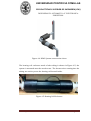
(shown in Figure 3.16). The duct sensor is a rod with a base attached to the
end of the unit. The tip of the rod is placed inside a duct to measure the
temperature. Duct sensors are common in areas where a wall mounted
sensor may be tampered with or damaged. They can be placed out of sight, in
the return duct of a room.
Part I. Report
Página 36
UNIVERSIDAD PONTIFICIA COMILLAS
ESCUELA TÉCNICA SUPERIOR DE INGENIERÍA (ICAI)
INGENIERO EN AUTOMÁTICA Y ELECTRÓNICA
INDUSTRIAL
Figure 3.16: Siemens Room Temperature Sensor (Left) and Duct
Temperature Sensor (Right)
An air quality sensor (QPA2000), refer to Figure 3.17, is important for
determining the level of CO2 in a room. It determines the amount of CO2 in
parts per million (ppm) and creates a 0 to 10 VDC linear proportional output
signal. The sensor has a range of 0 to 2000 ppm. Outside CO2 levels
generally vary between 300 and 400 ppm while room levels should not vary
higher than 600 to 700 ppm. If the level reaches 600 ppm in a room, then the
ventilation system needs to cycle fresh air throughout the enclosed
environment.
Figure 3.17: Air Quality Sensor (CO2)
Relative humidity can be measured using the sensor in Figure 3.18
(QFA3171D). This high accuracy device can measure temperature from 0C to
50C 32F to 22F) and relative humidity from 0 to 100%. The device outputs
Part I. Report
Página 37
UNIVERSIDAD PONTIFICIA COMILLAS
ESCUELA TÉCNICA SUPERIOR DE INGENIERÍA (ICAI)
INGENIERO EN AUTOMÁTICA Y ELECTRÓNICA
INDUSTRIAL
a signal of between 4 to 20 mA for the temperature and relative humidity
levels.
Figure 3.18: Relative Humidity/Temperature Sensor
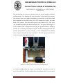
To actuate the damper in the model Variable Air Volume (VAV) box, shown in
Figure 3.19, an Actuating Terminal Equipment Controller (ATEC) is used
(550-405). This unit contains an actuator that controls a damper as well as
has two AIs and two DOs for other components. The controller also features a
high/low pressure differential sensor and a connection for a room or duct
temperature sensor.
Figure 3.19: Variable Air Volume Box (Left) and Actuating Terminal
Equipment Controller (Right).
Wiring the components depends on the different types of signals being
outputted to the controller. All the temperature sensors work by varying
resistance, which requires an AI on the controller. However the override
button on the room temperature sensor unit sends either a high or a low
Part I. Report
Página 38
UNIVERSIDAD PONTIFICIA COMILLAS
ESCUELA TÉCNICA SUPERIOR DE INGENIERÍA (ICAI)
INGENIERO EN AUTOMÁTICA Y ELECTRÓNICA
INDUSTRIAL
signal, therefore requiring a DI on the controller. The relays are connected to
the dry contact DOs with 24 VAC feeding them from the transformer. When
the DOs are triggered, the connection is closed and electricity from the
transformer activates the coils on the relays.
The humidity and CO2 sensor vary current and voltage, respectively, so they
both require AIs on the controller. The fire pull station consists of a button
that is constantly depressed until triggered by a user. When the user pulls
the fire alarm, the button is no longer depressed, therefore creating a closed
connection to a DI on the controller.
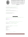
There are several programs, written in Insight, that are required to run some
of the components on the Siemens display board. These programs tell the
controller what to do with the I/Os. For instance, the Fire Pull Switch
Program tells the controller to enable an output when it receives an input. In
other words when a user pulls the fire alarm, the controller detects the input
from the button on the fire station and enables the output to the siren, as well
as turns off the VAV box fan to prevent the circulation of smoke.
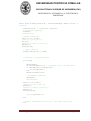
The next program is the Occupancy Switch Program. This program simulates
a person walking into the room. When the switch is flipped on, the system
knows someone is present and turns on the HVAC system, the fan in the VAV
box and slightly rotates the damper in the VAV box. The programs can be
viewed the Appendix (Figure 1.1 and 1.2, Chapter 1).
3.5
Guide User Interface (GUI)
The GUI subsystem is designed to allow any user to interface with the entire
system and learn about control system with ease. What separates the design
of TOCOM lab from other controls laboratories is the ability to interact with
the system via the GUI.
Part I. Report
As a result the GUI must meet the following
Página 39
UNIVERSIDAD PONTIFICIA COMILLAS
ESCUELA TÉCNICA SUPERIOR DE INGENIERÍA (ICAI)
INGENIERO EN AUTOMÁTICA Y ELECTRÓNICA
INDUSTRIAL
specifications and the chosen GUI design to meet those specifications is listed
below in Table 3.8.
Specifications
Display
Temperature,
Design
CO2,
and
Humidity
GUI has values displayed
Display Alerts and Alarms
Alerts and Alarms appear in GUI when triggered
All font must be at least 14pt
All descriptions of objects must have pictures included
All background colors must be easy to see colors (Blue, Red,
Green, Black, White)
A home button and a back arrow included on every page
with exception of first page
Easily navigatable GUI
Follow Ergonomic (Human Factor) standards for all graphs
Added a switch that turns entire VAV system to on position
Switch to activate VAV system
through Insight
Table 3.8: Specifications and Deliverables for GUI
The first major design decision was what program to run the GUI on to satisfy
all requirements. There are many options that were explored and, in some
cases, created to evaluate which program should be used (Simulink,
MATLAB). However for all the sensors to be integrated with the GUI the
program that should be used is Insight, a Siemens created program. Insight
displays all sensor values on a series of graphs along with the ability to
manage the overall system.
While Insight was chosen to create the GUI, it also had drawbacks that
needed to be modified for the program to accomplish all goals outlined.
Part I. Report
Página 40
UNIVERSIDAD PONTIFICIA COMILLAS
ESCUELA TÉCNICA SUPERIOR DE INGENIERÍA (ICAI)
INGENIERO EN AUTOMÁTICA Y ELECTRÓNICA
INDUSTRIAL
Insight’s major drawback was that it was designed for Siemens employees
and not meant to be user friendly. The program is built to store information
and allow anyone with knowledge of Siemens programming to access the
system. This was not acceptable as the GUI needed to be easy to use for
anyone not just those with an intimate knowledge of Insight. The solution
was found in Micrografx Designer, a program that interfaces with Insight that
allows for pictures, diagrams, schematics, and other more user friendly data
to be uploaded.
Now with the chosen programs in place the first step in the design was to
create a format that allows the system to be easily navigable and also outline
areas where sensor readings could be displayed along with all other relevant
information. To make sure the GUI could be used with ease the following
rules were applied to the design.
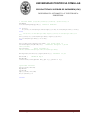
Now that these criteria had been established, the GUI homepage was created
as seen in Appendix (Figure 1.3, Chapter 1).
The rest of the pages were built with the next page called “First” that shows
all the different sensors and gives links that navigates to each sensor’s
reading (Refer to Appendix).
Each sensor page has the current value
displayed and if the user wishes for a larger window they can click on the
image.
Also on “First” is a link to the “Design” page which is created for a more indepth understanding of the system.
The “Design” page outlines each
individual component including a picture, description, price, and how it was
incorporated in the lab. The purpose of these pages is to show an engineer
how the system was built and how they could replicate the design in a system
that they would build. The design pages can be found in Figures 1.4-1.11 of
Appendix, Chapter 1.
Part I. Report
Página 41
UNIVERSIDAD PONTIFICIA COMILLAS
ESCUELA TÉCNICA SUPERIOR DE INGENIERÍA (ICAI)
INGENIERO EN AUTOMÁTICA Y ELECTRÓNICA
INDUSTRIAL
Once all pages were created a new problem surfaced, navigating through the
pages. Any person who has experience with Insight found this process easy,
but when a sample of students were shown the GUI as it was at that time, not
one could see an easy way to go back through the pages.
Given this
information, it was decided that two buttons should be placed at the top right
and left of each screen that gives the user the option to go back to the last
page (shown by a green arrow in the top left corner) and return back to the
homepage (shown by a House in the top right corner). The images for each
navigational button are shown below in Figure 3.20.
Figure 3.20 Back and Home buttons
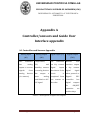
To meet the design goal of displaying the values, we first created point
addresses. These point addresses assign each sensor a point that is called in
the GUI to display the reading from that sensor. When a user clicks on a
sensor, the readings from that sensor are sent to the point created and
subsequently displayed on the page. The points created are seen in Figure
3.21.
Part I. Report
Página 42
UNIVERSIDAD PONTIFICIA COMILLAS
ESCUELA TÉCNICA SUPERIOR DE INGENIERÍA (ICAI)
INGENIERO EN AUTOMÁTICA Y ELECTRÓNICA
INDUSTRIAL
Figure 3.21: Created Points Menu
With the pages built and sensors integrated, we created alarms for each
sensor to message the user if the values are out of acceptable ranges. For
example if the reading for the CO2 sensor exceeds 600 parts/million an alarm
appears on screen informing the user that the value is too high. An example
of what the user observes can be found in Figure 1.12 Appendix, Chapter 1.
The next specification says that a shutdown button/ occupancy switch should
be able to turn the system on and off. This means that a switch is placed on
the board that when turned to the on position the VAV begins to push air
through the system and when turned to the off position no air flows through
the system. To meet this goal, a switch is placed in the system that when
turned on causes the VAV to turn on. When turned on, the VAV box begins to
turn the damper and the fan switches on. The temperature sensor in the VAV
also changes values which are displayed on the screen.
Part I. Report
Página 43
UNIVERSIDAD PONTIFICIA COMILLAS
ESCUELA TÉCNICA SUPERIOR DE INGENIERÍA (ICAI)
INGENIERO EN AUTOMÁTICA Y ELECTRÓNICA
INDUSTRIAL
Chapter 4
Implementation
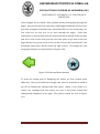
4.1 Construction
The TOCOM Mobile Cart has been constructed to the design specifications
described earlier. The CAD rendering of the unit, with primary components of
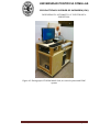
all systems is shown in Figure 4.1. The completed construction is shown in
Figure 4.2 and 4.3.
Figure 4.1: CAD Rendering of the TOCOM Mobile Lab
Part I. Report
Página 44
UNIVERSIDAD PONTIFICIA COMILLAS
ESCUELA TÉCNICA SUPERIOR DE INGENIERÍA (ICAI)
INGENIERO EN AUTOMÁTICA Y ELECTRÓNICA
INDUSTRIAL
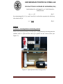
Figure 4.2 Photograph of TOCOM Mobile Lab, air control system and HVAC
system
Part I. Report
Página 45
UNIVERSIDAD PONTIFICIA COMILLAS
ESCUELA TÉCNICA SUPERIOR DE INGENIERÍA (ICAI)
INGENIERO EN AUTOMÁTICA Y ELECTRÓNICA
INDUSTRIAL
Figure 4.3: Photograph of the TOCOM Mobile Lab featuring Siemens
Component Display
HVAC System Construction
The main body of the HVAC system through which the air travels is made of
PVC tubing. All tubing was purchased in two feet lengths and then cut to size
using a horizontal band saw. Pipe cement was used to connect some portions
of the system while others were pressed together to allow for disassembly
and maintenance. Figure 4.4 shows a computer model of the entire system.
This figure was chosen over a picture of the physical system because the
system cannot stand free on its own.
Part I. Report
Página 46
UNIVERSIDAD PONTIFICIA COMILLAS
ESCUELA TÉCNICA SUPERIOR DE INGENIERÍA (ICAI)
INGENIERO EN AUTOMÁTICA Y ELECTRÓNICA
INDUSTRIAL
Figure 4.4: HVAC System construction: ducts
The heating coil enclosure made of abs tubing is shown in Figure 4.5; the
system is mounted onto the wooden cart. The brown wires running into the
tubing are used to power the heating coil housed inside.
Figure 4.5: Heating Coil Enclosure
Part I. Report
Página 47
UNIVERSIDAD PONTIFICIA COMILLAS
ESCUELA TÉCNICA SUPERIOR DE INGENIERÍA (ICAI)
INGENIERO EN AUTOMÁTICA Y ELECTRÓNICA
INDUSTRIAL
Fan and heating coil used were mounted into the system using an adhesive
insulation tape. The heating coil came incased in a heat shield (not shown).
The adhesive tape was wrapped around the circumference of each device and
then installed into the ABS tubing. The PVC tubing was used as the main
body of the system. The valve and cap were also made of PVC. The valve,
cap, and ABS fan housing are shown in Figure 4.6. The system in this figure is
in the standard flow configuration meaning the system would be taking in
outside air, circulating it through the system, and then dumping back into the
outside environment if it were running. In this configuration the exhaust
valve is open while the end cap is attached. The end cap prevents hot air
from running back through the system.
Figure 4.6: System in Standard Flow Configuration
In a reheat configuration the system re-circulates air from the box some of
the air from the box. In this configuration, the exhaust valve is closed while
Part I. Report
Página 48
UNIVERSIDAD PONTIFICIA COMILLAS
ESCUELA TÉCNICA SUPERIOR DE INGENIERÍA (ICAI)
INGENIERO EN AUTOMÁTICA Y ELECTRÓNICA
INDUSTRIAL
the end cap is removed thus allowing the air to be re-circulated and reheated.
The reheat configuration is shown in Figure 4.7.
Figure 4.7: System in Reheat Configuration
The differential pressure gage is shown in Figure 4.8 through the clear wall of
the cart. The gage is mounted inside the enclosed environment and measures
the differential pressure in the system. (Note: Further information on the
differential pressure gage can be found in both the Design and Analysis
section and the Testing section)
Part I. Report
Página 49
UNIVERSIDAD PONTIFICIA COMILLAS
ESCUELA TÉCNICA SUPERIOR DE INGENIERÍA (ICAI)
INGENIERO EN AUTOMÁTICA Y ELECTRÓNICA
INDUSTRIAL
Figure 4.8: Differential Pressure Gage
Lengths of clear tubing, which are used as the probes for the differential
pressure gage, installed in the system and attached to the back of the
differential pressure gage, are shown in Figure 4.9. The metal pipe seen
running into the PVC tubing is used to hold the total pressure probe parallel
with the flow of air.
Figure 4.9: Probes Connected to System and Differential Pressure Gage
Part I. Report
Página 50
UNIVERSIDAD PONTIFICIA COMILLAS
ESCUELA TÉCNICA SUPERIOR DE INGENIERÍA (ICAI)
INGENIERO EN AUTOMÁTICA Y ELECTRÓNICA
INDUSTRIAL
4.2 Testing
4.2.1 TOCOM Mobile cart
The TOCOM Mobile Cart was tested in a few specific areas concerning
mobility and support of onboard subsystems. The testing method and results
are outlined in Table 4.1.
Evaluation of
Customer Requirements
Testing
Results
Enclosed environment enabling Temperature increase without gross
temperature control
loss of heat input
Portable lab unit to be used Maintained assembly and mobility
throughout Loma Hall
while moving through Loma Hall
Stores and provides space for
onboard
computer
used
for
control of subsystems
All
computer
Provides space for demonstration
of Siemens components
can
function and be interfaced with
Provides space for onboard HVAC Observe
and air-recycling loop
components
that
HVAC
system
functions in the provided space
Pass
Pass
Pass
Pass
Siemens components fit within the
allotted space, allowing easy access Pass
for demonstration
Table 4.1: Testing Methods and Results for Mobile Cart
The primary focus of the testing for the TOCOM Mobile Cart was on mobility.
The cart was moved through engineering laboratories and onto the elevator
in the building; the successful transportation of the lab shows that the
requirement is met.
Part I. Report
Página 51
UNIVERSIDAD PONTIFICIA COMILLAS
ESCUELA TÉCNICA SUPERIOR DE INGENIERÍA (ICAI)
INGENIERO EN AUTOMÁTICA Y ELECTRÓNICA
INDUSTRIAL
The design of the system accounted for the space needed by the supported
subsystems; this requirement was met upon the completion of construction.
All components for the other subsystems fit on the cart and were positioned
to facilitate user interaction.
The integrity of the enclosed environment has been confirmed by the
successful addition of heat into the air within the system without excessive
heat loss, enabling the control system to achieve a steady-state temperature.
Heat loss within the system was unavoidable and necessary to achieve steady
state at an elevated temperature. Achieving the steady-state condition at an
elevated temperature demonstrates the functionality necessary for the
thermal systems and control systems lab exercises. An excessive loss of heat
would have prevented the system from reaching an elevated temperature,
indicating leakage of the air in the enclosure. Efficiency of the system was
revealed in the testing of the thermal systems lab.
4.2.2 HVAC
Throughout the project the team has continuously tested and adjusted the
design and parameters of the HVAC System. The system configuration has
been redesigned a total of four times. The first system contained automated
valves but through testing it was determined that the system could not
achieve the necessary pressure for the valves to function properly. The
second system was a similar layout to the first but contained all hand
actuated T-valves, requiring manual system adjustment.
As testing was
conducted on this system the team found that the fan being used could not
withstand the high temperature of the exhaust at the inlet and as a result the
team burned out a fan. The team then designed a system utilizing a Daton AC
Axial Fan which could tolerate a high inlet temperature. Although the fan was
rated for 115 cubic feet per minute (CFM) flow team found through testing
Part I. Report
Página 52
UNIVERSIDAD PONTIFICIA COMILLAS
ESCUELA TÉCNICA SUPERIOR DE INGENIERÍA (ICAI)
INGENIERO EN AUTOMÁTICA Y ELECTRÓNICA
INDUSTRIAL
that the fan did not provide a measureable pressure differential as required
by the labs. The finalized HVAC design uses a hair dryer fan at an open inlet
and utilizes an open air mixing process for the exhaust allowing for a lower
inlet air temperature during a reheat cycle.
To test the finalized HVAC system design the team took the customer
requirements and developed testing procedures for each one to evaluate the
team’s level of success. Table 4.2 below outlines the requirements, testing
procedures, and resulting outcome from each test.
Customer
Requirements
Ability to provide
a constant,
measurable flow
rate.
Ability to heat air
from room
temperature to 33
degrees Celsius
System withstands
temperature of
heating element
System fits inside
cart
System must be
function as both
standard and
reheat flow
Testing Procedure
Evaluation
Conduct a series of tests in which the system is run
using different temperature specifications set in
LabVIEW. During tests observe the differential
Pass
pressure gage to determine if there is a significant
change in pressure, indicating a change in flow rate.
Run the system at its maximum allowed temperature
set (33 degrees Celsius). Using the reading from the
Pass
thermocouple determine if the system reaches the set
temperature.
Heating element contained inside ABS piping which
is rated up to 76.7 degrees Celsius which exceeds the
elements maximum temperature. Run the system at
its maximum allowed temperature set (33 degrees
Pass
Celsius). Observe system to see if any deformations
form. (Note PVC piping is rated to 60 degrees
Celsius)
System designed to fit inside and on cart 25” x 50” x
Pass
32”. System was built and then installed onto the cart.
Test valves first by turning red handles to ensure they
rotate a full 90 degrees. Then conduct Thermal
Systems Lab written for this lab equipment
Pass
Table 4.2: HVAC Testing
Part I. Report
Página 53
UNIVERSIDAD PONTIFICIA COMILLAS
ESCUELA TÉCNICA SUPERIOR DE INGENIERÍA (ICAI)
INGENIERO EN AUTOMÁTICA Y ELECTRÓNICA
INDUSTRIAL
To test the ability of the HVAC system to provide a constant flow rate the
team ran a series of tests using ten different user specified temperatures in
LabVIEW. Each test took a different amount of time because the system had
to reach a different temperature each time.
Once a test began a team
member watched the differential pressure gage. If the reading on the gage
had changed it would have indicated a change in flow rate. In each of the
tests the readings from the differential pressure gage remained constant and
thus the flow rate remained constant. During these tests the team was also
adjusting the amount of power provided to the fan. The team found that at
very high speeds the controlled environment would not heat up because too
much air was running over the heating coil rendering it ineffective. When the
fan was running too slowly the heating coil would begin to get too hot.
During one of the tests the team burnt out a heating coil because there was
not enough air flowing through the system. The team determined that the
fan powered at 24 volts provides a flow rate of 14.7 CFM through the system.
This flow rate allows for the system to react quickly while not flooding the
heating coil with too much air.
The operator verified before testing the system that the valve and cap
worked properly. When testing for the maximum temperature the system
could achieve, the team found that that the system in the reheat configuration
achieved a higher maximum temperature than the system could in the
standard flow configuration. The maximum temperature the system can
achieve for the reheat configuration was found to be 37.5 degrees Celsius.
The maximum temperature the system can achieve for standard flow was
found to be 35.75 degrees Celsius. The team decided that for the lab there
should be a cap on how high students can set the temperature that does not
reach the maximum the system can achieve; thus in the lab the highest
temperature set is 33 degrees Celsius. The team decided to do this because it
Part I. Report
Página 54
UNIVERSIDAD PONTIFICIA COMILLAS
ESCUELA TÉCNICA SUPERIOR DE INGENIERÍA (ICAI)
INGENIERO EN AUTOMÁTICA Y ELECTRÓNICA
INDUSTRIAL
takes close to twenty minutes for the system to reach its max temperature;
where as it takes less than ten minutes to reach a steady state at 33 degrees
Celsius.
Operating Point
Differential
Pressure
Flow
Rate
Inches W.C.
0.4
0.5
0.6
0.7
0.8
0.9
1
1.1
1.2
1.3
1.4
1.5
CFM
9.839609
11.00102
12.05101
13.01658
13.91531
14.75941
15.55779
16.31715
17.0427
17.73861
18.40822
19.05432
Table 4.3: Differential Pressures and Corresponding Flow Rates.
Throughout all of the tests, including the maximum temperature tests, the
housing for the fan and heat coil as well as the piping stayed intact and
without any type of structural failure.
4.2.3 Controls
The running of the real system has been accomplished: effective gathering of
information transmitted by the sensors, transmission of control signals,
actuators powered by relay/transformers, and implementation of the final
controller in LabVIEW. Table 4.4 shows all the specifications with their
corresponding testing procedure.
Part I. Report
Página 55
UNIVERSIDAD PONTIFICIA COMILLAS
ESCUELA TÉCNICA SUPERIOR DE INGENIERÍA (ICAI)
INGENIERO EN AUTOMÁTICA Y ELECTRÓNICA
INDUSTRIAL
Specifications
Testing
Correct
Evaluation
between Pass
interfacing
components:
temperature
acquisition (thermocouples) and
transmission of control signals
through the DAQ. See if the values
Accurate integration of components in gathered in LabView match with
the control system
the real values.
Implementation
two Pass
of
transformers that provide 48 and
24 volts to power coil and fan. Test
Provide enough power to the actuators of the appropriate running of the
( fan, coil)
components (pipes, coil, fan).
Test the reference PID controller Pass
and
see
if
requirements
Accurate control response
it
achieves
and
the
effectively
controls the temperature.
Distribute a survey to students 9/10
and and receive feedback.
Intuitive interface using LabView
Table 4.4: LabVIEW Design Specifications and Testing.
4.2.4 Control systems lab
The controls lab has been tested separately from the overall controls systems
and the results are seen below in Table 4.5.
Part I. Report
Página 56
UNIVERSIDAD PONTIFICIA COMILLAS
ESCUELA TÉCNICA SUPERIOR DE INGENIERÍA (ICAI)
INGENIERO EN AUTOMÁTICA Y ELECTRÓNICA
INDUSTRIAL
Specifications
Testing
Evaluation
Compare the outcomes of the Pass
linear and non linear system and
Provide a tool that identifies the see if they are reasonable (less
transfer function of the system.
than 10% error between them).
Test
the
file
for
the Pass
following requirements:

Overshoot of 20%

Stability margins of at least
(distance
Provide
a
tool
that
gives
PID
controller
for
from x, y axis.)
the
parameters and expression of a certain
of

Quickest settling and rise
time for these limitations.
specific
requirements.
Test
the
real
system
and Pass
simulation for different values of
the PID controller.
Bring the possibility to export the
results in Matlab to Labview and see
the differences between simulation
and real system.
Attempt of the team members to Pass
Friendly guide to do the lab
do the lab in their own.
Table 4.5: MATLAB Specifications and Testing.
Part I. Report
Página 57
UNIVERSIDAD PONTIFICIA COMILLAS
ESCUELA TÉCNICA SUPERIOR DE INGENIERÍA (ICAI)
INGENIERO EN AUTOMÁTICA Y ELECTRÓNICA
INDUSTRIAL
The plant of the system is an integrator affected by a non-linear effect of the
actuator. This means that the response tends to be infinity in open loop, so it
is necessary to close the loop and proceed with an identification of the plant.
The file that originally was developed for the linearization was based on the
commands ‘trim’ and ‘linmod’ in Matlab, but unfortunately they can only be
applied to stable systems in open loop. To correct this problem a new file was
created, so it has been possible to do the identification. It is based on the
application of an iterative algorithm that solves the parameters of the
transfer function for a given input/output obtained from the non linear
system simulation.
Testing successfully reached the expectations. The PID controller, that the file
in Matlab gives, has been tested and checked manually for the same
specifications indicated above in Table 4.5.
The sample lab guide that students will be performing can be found in
Appendix, Chapter 3.
Finally, both simulation and real system responses have been gathered and
compared to ensure that the identification is accurate. Both responses were
exported to an excel file as shown in Figure 4.10.
Part I. Report
Página 58
UNIVERSIDAD PONTIFICIA COMILLAS
ESCUELA TÉCNICA SUPERIOR DE INGENIERÍA (ICAI)
INGENIERO EN AUTOMÁTICA Y ELECTRÓNICA
INDUSTRIAL
Comparison real system(LabVIEW)-simulation(Matlab)
Temperature (⁰C)
30,5
Simulation
(Matlab)
30
29,5
Real
system
(LabVIEW)
29
28,5
28
27,5
0
50
100
150
200
Time(sec.)
Figure 4.10 Comparison real system (LabVIEw)-simulation (Matlab)
As it can be inferred from Figure 4.10, the approach to the real system made
by the system identified is accurate. The PID reference-cotroller mentioned
in chapter 3 was implemented to obtain these responses (Kp=10, Ki=0.1,
Kd=0.01). Both responses show a similar shape and reach the steady state at
the same time but they present different rising times. One of the possible
causes of these differences may be an error in some of the parameters
involved in the identification such as the convection factor or the dimensions
of the coil (mass, volume, etc.). Furthermore, the fact that 4 thermocouples
have been used may not be enough to calculate an accurate average
temperature.
Although of these inconvinients, the model is accurate enough to proceed
with the development of the labs.
Part I. Report
Página 59
UNIVERSIDAD PONTIFICIA COMILLAS
ESCUELA TÉCNICA SUPERIOR DE INGENIERÍA (ICAI)
INGENIERO EN AUTOMÁTICA Y ELECTRÓNICA
INDUSTRIAL
4.2.5 Thermal systems lab
Testing of the Thermal Systems Lab was focused on ensuring a smooth
completion of the laboratory exercise. Points of interest in testing included
the ease of operation of the TOCOM mobile unit, ability to gather relevant
data, and clear instructions for calculation of efficiency.
Volunteer
engineering students were asked to perform the lab by following the
directions provided by the lab handout. They were then asked to complete a
survey form, tailored to gauge the success of the lab in each of the testing
areas (The form is included in the Appendix, Chapter 2). The testable areas
are illustrated in Table 4.6.
Evaluation of
Customer Requirements
Thermal
systems
students
to
lab
compare
enables
power
savings due to recycling loop
Testing
Results
After
Lab test volunteers followed the 100%
of
temperature
and in controlled space by
LabVIEW software
provided
to
to
measure
fan
element
and
power Lab
test
volunteers
100%
of
could
users
take
temperature
readings
using
LabVIEW
gave
100%
heating feedback on success of capture could
system
Ability to measure differential Lab
Part I. Report
users
lab successfully
Temperature readings before and measurements of air at source
Ability
of
lab procedure and gave feedback could complete the
Acquisition
after addition of heat
revision,
of
export
users
the
data from LabVIEW
test
volunteers
gave
After
Página 60
revision,
UNIVERSIDAD PONTIFICIA COMILLAS
ESCUELA TÉCNICA SUPERIOR DE INGENIERÍA (ICAI)
INGENIERO EN AUTOMÁTICA Y ELECTRÓNICA
INDUSTRIAL
pressure through the system, and feedback on success of mass 100%
use for mass flow rate calculation
flow rate calculation
of
users
correctly calculated
the flow rate
Lab exercise can be completed
without excessive time to reach
temperature set points
Lab
test
volunteers
gave
feedback on the length of time Average
required
to
complete
of
7
the minutes to reach
exercise
Initial fail, error in
equations
Lab exercise can be completed Lab
test
with only instructions provided by feedback
the lab handout
volunteers
on
was
gave revealed,
after
successful revision 100% of
completion of the exercise
users
correctly
could
calculate
the efficiencies
Table 4.6: Requirements Testing for Thermal Systems Lab.
The design and configuration of the TOCOM Mobile Lab was dependent on
the successful integration of the HVAC system and air temperature control
system.
The thermal systems lab exercise utilizes all three properly
integrated subsystems, allowing for the efficiency analysis of both the open
and closed system configurations.
Thermocouple sensors were properly installed and interfaced with LabVIEW
enabling users to collect and view the temperature measurement data. The
reading was initially found to be inaccurate by 3 ºC, but it was calibrated
using a thermocouple heat meter. The sensors, one measuring upstream of
the heating element and one inside the controlled space, provide a
temperature differential which is acquired and recorded by LabVIEW. The
Part I. Report
Página 61
UNIVERSIDAD PONTIFICIA COMILLAS
ESCUELA TÉCNICA SUPERIOR DE INGENIERÍA (ICAI)
INGENIERO EN AUTOMÁTICA Y ELECTRÓNICA
INDUSTRIAL
power provided to the system fan and heating element is also recorded in
LabVIEW. Upon testing the lab exercise, the users were able to extract all
data required for the efficiency analysis.
Mass flow rate of the air through the air temperature control system is
calculated from the differential pressure gauge measurement. Though this
was possible upon testing the lab, it was discovered that the lab handout did
not include the equation for mass flow rate calculation from a pressure
differential.
This created a problem as the lab exercise could not be
completed using only the lab handout as a reference.
The necessary
corrections were made to the lab handout.
The objective of the thermal systems lab is to compare the performance of
the two system configurations by analyzing efficiency.
The values of
efficiency for some configurations are displayed in Table 4.7.
Set Point
Configuration
Efficiency
27
open
43.60%
27
reheat
53.50%
33
open
62.45%
33
reheat
43.90%
Table 4.7: Efficiency of the air temperature control system
Note that the efficiency decreases for the system with reheat compared to the
open system at 33 ºC. This indicates the optimum operating point for the
reheat configuration is below 33 ºC. Time to meet these temperature set
points was 7 minutes on average, enabling the completion of the lab without
excessive downtime.
Part I. Report
Página 62
UNIVERSIDAD PONTIFICIA COMILLAS
ESCUELA TÉCNICA SUPERIOR DE INGENIERÍA (ICAI)
INGENIERO EN AUTOMÁTICA Y ELECTRÓNICA
INDUSTRIAL
4.2.6 Controller and sensors
Table 4.8 shows the tests that were conducted on the system. The first test
conducted was to make sure that the fire strobe light flashes when the fire
pull switch is triggered. This was tested by first examining the program
before uploading it to the controller, making sure the correct variables were
utilized and that the code was able to be compiled. Then the fire pull switch
was triggered by pulling the white lever on the sensor backboard. The test
was a success on the first attempt, due to the correct labeling of variables and
understanding of code.
Key Customer Requirements
Fire pull switch enables strobe
light
Room
occupancy
wall
switch
enables fan
Fire pull switch program disables
fan when pulled
Testing Procedure
Pulled fire alarm
Pass
Flip wall switch on
Pass
Pulled fire alarm
Pass
ATEC moves the damper in the Command the ATEC to rotate the
VAV box
damper 50%
Sensors visible to all users
Outcome
Multiple
people
of
Pass
different 4/5
heights viewed the system
people
passing score
Table 4.8: Controller and Sensor Testing
The room occupancy switch was tested in a very similar manner as the fire
pull switch. A program was created that enables the appropriate variable
Part I. Report
Página 63
gave
UNIVERSIDAD PONTIFICIA COMILLAS
ESCUELA TÉCNICA SUPERIOR DE INGENIERÍA (ICAI)
INGENIERO EN AUTOMÁTICA Y ELECTRÓNICA
INDUSTRIAL
when the switch on the sensor backboard is triggered. This program is
similar to that of the fire pull program so it also worked on first try.
The next test was tougher to get a positive result due to being slightly more
complex. The first dozen tests failed due to the code. The variables and
installation were all correct, however the code structure was more difficult to
understand due to the old FORTRAN based code. The conditional statement
had to be aware of multiple scenarios instead of the conventional single
scenario. The controller needed to be able to differentiate whether the fan
was on when the fire alarm was triggered. In real life situations, if the fire
alarm is triggered in a building the system shuts down the HVAC system so
that smoke is not distributed throughout the ventilation. After much
programming, it became clear that a single multi-conditional statement was
all that was needed.
The fourth test was to make sure that the ATEC was correctly installed onto
the VAV box and wired to the FLN network to communicate with the main
PXC controller. The ATEC has a built in actuator that rotates the damper in
the VAV box to limit the airflow. The first test on the device was to make sure
the ATEC was able to rotate the damper when given a command from a
computer directly plugged into it. After that succeeded, the device was
connected to the PXC controller through the FLN network and a command
was sent from the desktop computer running Insight instructing the device to
rotate the damper 50% (about a 45 angle). This, to some surprise, worked
without hesitation, proving the successful installation and networking of the
ATEC.
The last test conducted on the system was to make sure users of all heights
could easily see all the sensors on the backboard. Five individuals were
selected based on a variety of heights (ranging from 5 foot 3 inches to 6 foot 3
inches) and asked to examine the sensor backboard. Four out of the five
Part I. Report
Página 64
UNIVERSIDAD PONTIFICIA COMILLAS
ESCUELA TÉCNICA SUPERIOR DE INGENIERÍA (ICAI)
INGENIERO EN AUTOMÁTICA Y ELECTRÓNICA
INDUSTRIAL
people could see all the components on the backboard with ease. One person
had a slight difficulty reading the display of the temperature/humidity sensor
in the top left corner of the board. Fortunately the values for that sensor can
be found in the GUI.
4.2.7 Guide User Interface (GUI)
Customer Requirements
Display
Testing Procedure
Results
Temperature, Observe the displayed results Pass
CO2, and Humidity
and
test
with
temperature
separate
another
sensor
system
to
on
verify
results
Easily Navigable GUI
Distribute a survey to students 90% (18/20)
and
team
members
and
receive feedback
Switch to Activate VAV Turn on switch and see if fan Pass
system
turns on and observe if the
values on the GUI reflect this
change
Display
Alerts
Alarms
and Watch the values exceed the Pass
set limit and observe if an
alarm is activated
Table 4.9: Testing Procedure and Results for GUI
The display of temperature and other values are tested by observing if the
system is in fact displaying values. To ensure that those values are correct
Part I. Report
Página 65
UNIVERSIDAD PONTIFICIA COMILLAS
ESCUELA TÉCNICA SUPERIOR DE INGENIERÍA (ICAI)
INGENIERO EN AUTOMÁTICA Y ELECTRÓNICA
INDUSTRIAL
other separate sensors measure the temperature and the results are
compared to verify the correct values. The results show that the system does
in fact display the Temperature, CO2, and Humidity values.
The alerts and alarms are tested by making the values exceed the set
guidelines for too high and observing if the alarm goes off. The results show
that the alerts and displays do in fact alert the user when they get past the set
limit off acceptable ranges.
The VAV system turning on by a switch is tested by turning the switch and
observing if the system has been turned on. The temperature should change
in the GUI when the switch turns on and to be sure that the system is
functioning, the display reflects that change in temperature. The results
show that the system does in fact respond to the switch when it has been
activated.
The GUI itself needs to be user friendly and this is tested by having students
and group members work through the GUI and take a survey to express what
they liked, disliked, and suggestions for improvement. After students took
the survey their results showed that overall the GUI has attained its goal of
being easy to navigate and aesthetically pleasing. Some comments about
improvement oriented around the need for a Home and Back button on each
page, the button layout on the first screen needs to be larger, and the
descriptions for parts text needs to be larger. All these suggestions were
taken into account and changes to the GUI reflect that input. The surveys
were administered on April 30- May 3/2011 to 17 engineering students and
3 non-engineering majors.
Part I. Report
Página 66
UNIVERSIDAD PONTIFICIA COMILLAS
ESCUELA TÉCNICA SUPERIOR DE INGENIERÍA (ICAI)
INGENIERO EN AUTOMÁTICA Y ELECTRÓNICA
INDUSTRIAL
References
[1]F.Luis Pagola; Control Digital; Universidad Pontificia Comillas.
[2]F.Luis Pagola; Regulación Automática; Universidad Pontificia Comillas.
[3]Frank P.Incropera, David P.De Witt;”Fundamentos de transferencia de
calor.
[4] National Instruments; www.ni.com.
[5]Isaac Pérez Moreno; “Manual de prácticas de control avanzado utilizando
la tarjeta de adquisición de datos NI USB 6008”.
[6]Siemens;”APOGEE Actuating Terminal Equipment Controller: owners
manual”.
[7] Siemens; “Introducing the Zone Control Unit”.
Part I. Report
Página 67
UNIVERSIDAD PONTIFICIA COMILLAS
ESCUELA TÉCNICA SUPERIOR DE INGENIERÍA (ICAI)
INGENIERO EN AUTOMÁTICA Y ELECTRÓNICA
INDUSTRIAL
PART II
BUDGET
Part II. Budget
Página 68
UNIVERSIDAD PONTIFICIA COMILLAS
ESCUELA TÉCNICA SUPERIOR DE INGENIERÍA (ICAI)
INGENIERO EN AUTOMÁTICA Y ELECTRÓNICA
INDUSTRIAL
1. Budget
This section includes a detailed budget that has been required to succesfully
develop the Project.
Labor budget:
Considering an average engineer’s remuneration of 50
and 300 hours
of total work, the final cost is:
Hardware:
Tables 1.1 and 1.2 show a detailed part lists of both Siemens and HCAV
components with their corresponding prices.
QTY
1
1
1
1
2
1
2
1
1
1
1
1
1
1
1
2
1
1
1
1
5
1
1
1
Product Number
PXC100-PE.A
PXX-485.3
TXS1.12FA
TXM1.16D
TXM1.6R-M
TXM1.8U-ML
TXM1.8X-ML
550-405
540-100
536-811
540-128
QAM2012.010
533-376-4
QPA2000
QFA3171D
540-680FB
GDE131.1P
500-636173
141-0574
3VU69
RH1BU-AC24V
571-010-3P11-USB
538-670
Part Description
PXC Modular w/FLN & TX-I/O
Expansion Module, 3 RS-485 Connections
24VDC Supply
16 Digital Input Module
6 Digital Output Relay Module w/OVD
8 Universal I/O Module w/OVD & LCD
8 Universal I/O Module w/4-20mA, OVD & LCD
Actuating Terminal Equipment Controller (ATEC VAV)
Terminal Equipment Controller (TEC)
100K OHM TEC Thermistor Temperature Sensor
10K OHM TEC Thermistor Temperature Sensor
Platinum 1K OHM Duct Temperature Sensor
20-120°F 100 OHM Duct Temperature Sensor,4-20mA
CO2 Room Air Quality Sensor, 0-10V
Room Humidity/Temperature Sensor w/Display, 4-20mA
TEC Room Temperature Sensor w/STPT & Display
Open Air Actuator
Visual Strobe Light
Air Flow Switch, .05-1.0 WC
Dayton AC 239 CFM Axial Fan
SPDT 24VAC Relay w/base
Insight Advanced Server 1 User License
Trunk Interface
Dell Computer/Monitor
Retail Price
$7,097.22
$908.45
$560.00
$738.00
$1,113.89
$1,569.75
$1,847.22
$806.25
$647.95
$46.12
$50.80
$36.00
$155.45
$672.73
$750.00
$177.17
$278.22
$69.12
$119.98
$78.30
$4.75
$5,000.00
$806.36
$1,100.00
Total
Total
$7,097.22
$908.45
$560.00
$738.00
$2,227.78
$1,569.75
$3,694.44
$806.25
$647.95
$46.12
$50.80
$36.00
$155.45
$672.73
$750.00
$354.34
$278.22
$69.12
$119.98
$78.30
$23.75
$5,000.00
$806.36
$1,100.00
Siemens Price
$2,365.74
$302.82
$186.67
$246.00
$742.59
$523.25
$1,231.48
$268.75
$215.98
$15.37
$16.93
$12.00
$51.82
$224.24
$250.00
$118.11
$92.74
$23.04
$39.99
$26.10
$7.92
$1,666.67
$268.79
$366.67
$27,791.01
$9,263.67
Table 1.1: Siemens display parts list
Part II. Budget
Página 69
UNIVERSIDAD PONTIFICIA COMILLAS
ESCUELA TÉCNICA SUPERIOR DE INGENIERÍA (ICAI)
INGENIERO EN AUTOMÁTICA Y ELECTRÓNICA
INDUSTRIAL
Table 1.2 Parts list for HVAC components
The overall budget in hardware components for the project was $10,193.67.
The majority of the funding ($9,263.67) was provided by Siemens Industry
which included the computer and the components. USD Associated Students
(AS) also provided funding for the construction of the cart and wiring of the
HVAC system.
Software
To develope the Project the following programs have been required:
LabVIEW…………………………….150$
Matlab with Simulink………….. 50$
Part II. Budget
Página 70
UNIVERSIDAD PONTIFICIA COMILLAS
ESCUELA TÉCNICA SUPERIOR DE INGENIERÍA (ICAI)
INGENIERO EN AUTOMÁTICA Y ELECTRÓNICA
INDUSTRIAL
Microssoft Office 2007...………600$
Final cost=900$
In conclusión, the final budget adding labor, hardware and software is:
Part II. Budget
Página 71
UNIVERSIDAD PONTIFICIA COMILLAS
ESCUELA TÉCNICA SUPERIOR DE INGENIERÍA (ICAI)
INGENIERO EN AUTOMÁTICA Y ELECTRÓNICA
INDUSTRIAL
PART III
APPENDIX
Part III. Appendix
Página 72
UNIVERSIDAD PONTIFICIA COMILLAS
ESCUELA TÉCNICA SUPERIOR DE INGENIERÍA (ICAI)
INGENIERO EN AUTOMÁTICA Y ELECTRÓNICA
INDUSTRIAL
Appendix A
Controller/sensors and Guide User
Interface appendix
A.1 Controller and Sensors Appendix
Analog Input
Analog Output
(AI)
(AO)
PXC
has
Digital Input (DI)
(DO)
controller Temperature,
analog CO2,
PXC
controller Buttons
analog
and
and has dry contact switches output
inputs to receive Humidity sensors digital
signals
Digital Output
inputs a
dry
contact
from are analog devices that detect if the digital
devices that
(i.e. sensors)
output
linear
a circuit
signal
is when pressed or
analog completed from flipped.
PXC
4mA-20mA or 0V- one contact to controller
10V signal
the other
has
digital
outputs
for
ON/OFF
operation
an
enable relays
Table 1.1 Description of inputs and outputs
Part III. Appendix
Página 73
UNIVERSIDAD PONTIFICIA COMILLAS
ESCUELA TÉCNICA SUPERIOR DE INGENIERÍA (ICAI)
INGENIERO EN AUTOMÁTICA Y ELECTRÓNICA
INDUSTRIAL
Figure 1.1: Fire Pull Switch Program Flowchart
This program represents what happens when a real wall mounted fire pull station is
triggered in a building. When the alarm is triggered, a strobe light will flash, and an alarm
is displayed in the Insight software.
Point Declaration
Type
Description
TCM.SWT.01.FIRE
LDI
FIRE PULL SWITCH
TCM.ALM.01.FIRE
LDO
FIRE ALARM LIGHT/SIREN
00010
00020
00030
00040
00050
00060
C
C ---FIRE PULL ALARM--C
DEFINE(FIRE,"TCM.SWT.01.FIRE")
DEFINE(ALFIRE,"TCM.ALM.01.FIRE")
IF(%FIRE%.EQ.OFF) THEN OFF(%ALFIRE%) ELSE ON(%ALFIRE%)
Part III. Appendix
Página 74
UNIVERSIDAD PONTIFICIA COMILLAS
ESCUELA TÉCNICA SUPERIOR DE INGENIERÍA (ICAI)
INGENIERO EN AUTOMÁTICA Y ELECTRÓNICA
INDUSTRIAL
Figure 1.2 Occupancy Switch Program Flowchart
This program detects occupancy. In order for the system to be used, a switch will need to
be flipped (as if a person was to walk into a room or office). When a person enables the
occupancy switch, the fan in the VAV box turns on and the model damper starts rotating
to simulate the HVAC system responding the environment. If the Fire Alarm is enabled,
then the fan shuts off to prevent smoke circulation.
Point Declaration
Type
Description
TCM.AH1.01.DMPR
LAO
MODEL AIR HANDLING DAMPER
TCM.SWT.02.OCPY
LDI
OCCUPANCY SWITCH
TCM.VAV.01.FAN
LDO
VAV BOX FAN
00070
00080
00090
00100
C
C ---OCCUPANCY SWITCH--C
DEFINE(DMPR,"TCM.VAV.02.DMPR") ---Define Variables, variables called in
other programs do not need to be called again (i.e. FIRE)
00110 DEFINE(OCPY,"TCM.SWT.02.OCPY")
00120 DEFINE(FAN,"TCM.VAV.01.FAN")
00140
IF(%OCPY%.EQ.OFF.AND.%FIRE%.EQ.OFF).OR.(%OCPY%.EQ.ON.AND.%FIRE%.EQ.
ON).OR.(%OCPY%.EQ.OFF.AND.%FIRE%.EQ. ON) THEN OFF(%FAN%)ELSE
ON(%FAN%)
Part III. Appendix
Página 75
UNIVERSIDAD PONTIFICIA COMILLAS
ESCUELA TÉCNICA SUPERIOR DE INGENIERÍA (ICAI)
INGENIERO EN AUTOMÁTICA Y ELECTRÓNICA
INDUSTRIAL
A.2 Guide User Interface (GUI) Appendix
Figure 1.3: GUI Homepage
Part III. Appendix
Página 76
UNIVERSIDAD PONTIFICIA COMILLAS
ESCUELA TÉCNICA SUPERIOR DE INGENIERÍA (ICAI)
INGENIERO EN AUTOMÁTICA Y ELECTRÓNICA
INDUSTRIAL
Figure 1.4: First Page
Figure 1.5: Temperature Sensors Page
Part III. Appendix
Página 77
UNIVERSIDAD PONTIFICIA COMILLAS
ESCUELA TÉCNICA SUPERIOR DE INGENIERÍA (ICAI)
INGENIERO EN AUTOMÁTICA Y ELECTRÓNICA
INDUSTRIAL
Figure 1.6: Duct Temperature Sensor Page
Figure 1.7: Humidity/Temperature Readings
Part III. Appendix
Página 78
UNIVERSIDAD PONTIFICIA COMILLAS
ESCUELA TÉCNICA SUPERIOR DE INGENIERÍA (ICAI)
INGENIERO EN AUTOMÁTICA Y ELECTRÓNICA
INDUSTRIAL
Figure 1.8: CO2 Sensor Page
Figure 1.9: Beginning Page
Part III. Appendix
Página 79
UNIVERSIDAD PONTIFICIA COMILLAS
ESCUELA TÉCNICA SUPERIOR DE INGENIERÍA (ICAI)
INGENIERO EN AUTOMÁTICA Y ELECTRÓNICA
INDUSTRIAL
Figure 1.10: Design Page 2
Figure 1.11 Design Page 3
Part III. Appendix
Página 80
UNIVERSIDAD PONTIFICIA COMILLAS
ESCUELA TÉCNICA SUPERIOR DE INGENIERÍA (ICAI)
INGENIERO EN AUTOMÁTICA Y ELECTRÓNICA
INDUSTRIAL
Figure 1.12: Alarm page
Part III. Appendix
Página 81
UNIVERSIDAD PONTIFICIA COMILLAS
ESCUELA TÉCNICA SUPERIOR DE INGENIERÍA (ICAI)
INGENIERO EN AUTOMÁTICA Y ELECTRÓNICA
INDUSTRIAL
Appendix B: Thermal Systems Lab
users manual.
Table of contents
1
INTRODUCTION ............................................................................. 3
2
EQUIPMENT DESCRIPTION .......................................................... 4
3
NOMENCLATURE ........................................................................... 6
4
INVESTIGATION OF AIR HEATING SYSTEM ................................ 7
4.1
Part A ........................................................................................................8
4.2
Part B ...................................................................................................... 11
4.3
Results .....................................................................................................12
4.4
Conclusion .............................................................................................. 12
5
EXPERIMENTER CHECK LIST .................................................... 13
5.1 Thermal system lab survey form .............................................................. 14
Part III. Appendix
Página 82
UNIVERSIDAD PONTIFICIA COMILLAS
ESCUELA TÉCNICA SUPERIOR DE INGENIERÍA (ICAI)
INGENIERO EN AUTOMÁTICA Y ELECTRÓNICA
INDUSTRIAL
1.Introduction
The TOCOM Mobile Lab unit uses LabVIEW to run a control system which
regulates the air temperature in an enclosed environment. In the following
experiments the air temperature control system will be used to provide a
steady state temperature within the enclosed environment.
Increased efficiency is a primary motivation for many engineering
applications. By taking temperature, differential pressure, and electrical
power measurements the efficiency of the air temperature control system
can be calculated. The objective of the following experiment is to analyze and
compare the efficiency of (1) an open loop heating system (2) as well as a
heating system using reheat, or a recirculation of the heated air through the
system.
Part III. Appendix
Página 83
UNIVERSIDAD PONTIFICIA COMILLAS
ESCUELA TÉCNICA SUPERIOR DE INGENIERÍA (ICAI)
INGENIERO EN AUTOMÁTICA Y ELECTRÓNICA
INDUSTRIAL
2. Equipment Description:
The air temperature control system is physically composed of the enclosed
environment and the HVAC System (seen in Figure 1).
Figure 1 – HVAC System diagram
The control system allows the system devices (fan motor and electric
resistive heating coil within the HVAC loop) to be activated and configured
through the LabVIEW software.
Temperature data will be collected via
thermocouple sensors placed throughout the system and displayed through
Part III. Appendix
Página 84
UNIVERSIDAD PONTIFICIA COMILLAS
ESCUELA TÉCNICA SUPERIOR DE INGENIERÍA (ICAI)
INGENIERO EN AUTOMÁTICA Y ELECTRÓNICA
INDUSTRIAL
LabVIEW. A detailed diagram of the airflow and devices within the system
can be seen in Figure 2. T1 and T2 indicate the placement of the controlled
space temperature and inlet temperature respectively.
Figure 2 - HVAC circuit diagram
The valves can be set to two positions which change the system geometry
from (1) open without reheat to (2) open with reheat. By closing the reheat
valve, the system changes from configuration (1) to (2). The reheat system
valve configuration is shown in Figure 3.
Part III. Appendix
Página 85
UNIVERSIDAD PONTIFICIA COMILLAS
ESCUELA TÉCNICA SUPERIOR DE INGENIERÍA (ICAI)
INGENIERO EN AUTOMÁTICA Y ELECTRÓNICA
INDUSTRIAL
Figure 3 - Open valve configuration
Pressure is measured via a differential pressure gauge, which compares the
stagnation pressure and dynamic pressure of the air moving through the inlet
to the controlled space (see Figure 4).
Part III. Appendix
Página 86
UNIVERSIDAD PONTIFICIA COMILLAS
ESCUELA TÉCNICA SUPERIOR DE INGENIERÍA (ICAI)
INGENIERO EN AUTOMÁTICA Y ELECTRÓNICA
INDUSTRIAL
Figure 4 – Differential pressure gauge
3. Nomenclature:
Quantity
Current
Voltage
Power
Symbol
I
V
P
Units (SI)
A
V
W
Units (Imperial)
-
Pressure
p
(Pa) N/m2
inch WC
Volumetric Flow Rate
V
m /s
ft /s
Mass Flow rate
Density
m
ρ
kg/s
kg/m3
slugs/s
slugs/ft3
Efficiency
η
%
%
Specific heat
c
(kJ/kg)K
(Btu/lb)⁰R
Temperature
T
K
⁰R
volume which passes through pipe per
unit time
rate mass passes through pipe per unit
time
mass per unit volume
percentage of power retained from
input to outp t
amount of heat required to change
temperature
physical property of matter relating to
thermal equilibrium
h
kJ/kg
kJ/s
kJ/kg
Btu/lb
Btu/s
Btu/lb
rate of heat transfer per unit mass
rate of h at transfer per unit time
total energy of a thermodynamic system
Heat transfer
Enthalpy
Part III. Appendix
3
3
Description
flow of electric charge
electrical potential difference
rate of energy transfer
force exerted on a container per unit
area
Página 87
UNIVERSIDAD PONTIFICIA COMILLAS
ESCUELA TÉCNICA SUPERIOR DE INGENIERÍA (ICAI)
INGENIERO EN AUTOMÁTICA Y ELECTRÓNICA
INDUSTRIAL
4. Investigation of air temperature control system
Objective:
To determine the efficiency of the system at steady state by comparing power
input to heat output, and to compare the efficiency of the reheat
configuration to the open loop configuration.
Theory:
Efficiency of the heating system can be described by EQ. 1:
- EQ. 1
In this case, the ‘Qout’ is the rate of heat transferred to the air by the HVAC
system. The ‘Pin’ is the electrical power added to the fan and resistive
heating coil. The total electrical power can be calculated with EQ. 2.
- EQ. 2
The rate of heat added to the air in the system can be expressed by EQ. 3.
- EQ. 3
Mass flow rate can be calculated using differential pressure and some system
performance dependent constants.
The calculation can be performed
directly using EQ. 4.
where
EQ. 4
is the differential pressure (inches W.C.). The mass flow rate is in
SI units (
.
If the assumption is made that the air in the system is incompressible and can
be modeled as an ideal gas, the relationship described in EQ. 5 can be used.
This assumption is appropriate for this system’s analysis.
Part III. Appendix
Página 88
UNIVERSIDAD PONTIFICIA COMILLAS
ESCUELA TÉCNICA SUPERIOR DE INGENIERÍA (ICAI)
INGENIERO EN AUTOMÁTICA Y ELECTRÓNICA
INDUSTRIAL
- EQ. 5
By substituting EQ. 2, 3, 4, and 5 into EQ. 1 we find the equation for efficiency
described in EQ. 6.
- EQ. 6
Method:
4.1 Part A – Investigation of air heating system
Ensure the system geometry is in the open configuration by checking that the
exhaust valve is open and the end cap is placed on the reheat outlet (see
Figure 5).
Figure 5 - Open System Valve Configuration
Part III. Appendix
Página 89
UNIVERSIDAD PONTIFICIA COMILLAS
ESCUELA TÉCNICA SUPERIOR DE INGENIERÍA (ICAI)
INGENIERO EN AUTOMÁTICA Y ELECTRÓNICA
INDUSTRIAL
Check that power is supplied to the HVAC loop by ensuring the onboard
power strip is switched to the on position. Turn on the computer aboard the
TOCOM Mobile Unit and open the control system in LabVIEW by opening the
VI file via the following path:
Desktop >> TOCOM >> control_PID tocomlab.vi
Open the Thermal Systems tab to open the interface shown in Figure 6. This
interface will be used to activate the control system and simultaneously
monitor the instantaneous temperature and power measurements.
Figure 6 - Screenshot of LabVIEW interface
The control system which provides the steady-state temperature within the
system must be configured before beginning the experiment:
Part III. Appendix
Página 90
UNIVERSIDAD PONTIFICIA COMILLAS
ESCUELA TÉCNICA SUPERIOR DE INGENIERÍA (ICAI)
INGENIERO EN AUTOMÁTICA Y ELECTRÓNICA
INDUSTRIAL
Under the PID tab, enter the following values in their respective fields:
Kp=10
Ki=0.1
Kd=0.01
Under the PWM tab, enter the values in their respective fields:
Precision = 25
Rate Time = 5
Amplitude = 5
In LabVIEW under the PID tab, change the temperature set point
(desired_temp) to 28 ºC. Enable the control system by clicking the left
pointing arrow icon in the top left corner of the LabVIEW window. Allow the
system to reach steady-state temperature; this will be evident by a flat trend
in the temperature display (under Thermal Systems tab). Here the control
system will maintain the temperature in the controlled space by
intermittently actuating the heating coil. The fan should always be running.
While the enclosed space is being heated, record the pressure reading from
the differential pressure gauge within the controlled space, visible through
the controlled space window.
Once the temperature set point has been reached and the system is at steady
state (seen in Figure 7), use LabVIEW to collect temperature readings from
both the controlled space (T1), the air inlet (T2), and power supplied to the
fan and heating coil (note that for part A the inlet temperature T2 will be
room temperature).
Part III. Appendix
Página 91
UNIVERSIDAD PONTIFICIA COMILLAS
ESCUELA TÉCNICA SUPERIOR DE INGENIERÍA (ICAI)
INGENIERO EN AUTOMÁTICA Y ELECTRÓNICA
INDUSTRIAL
Figure 7 - Steady-state reading in LabVIEW
Measurements are displayed within the Thermal Systems tab, and can be
exported to Excel after the program has stopped running. Before collecting
data be sure to clear the current data by right-clicking each graph and
selecting ‘clear chart’. After sufficient data has been collected, stop operation
of the system by clicking the ‘stop process’ button. To extract data right-click
the graph displaying the desired data, select ‘Export’, then ‘Export Data to
Excel’. Excel will automatically open with the data displayed.
Collect data points for each temperature set point at 28, 30, and 33⁰C note
that the room temperature affects the speed to reach the set point).
Part III. Appendix
Página 92
UNIVERSIDAD PONTIFICIA COMILLAS
ESCUELA TÉCNICA SUPERIOR DE INGENIERÍA (ICAI)
INGENIERO EN AUTOMÁTICA Y ELECTRÓNICA
INDUSTRIAL
4.2 Part B – Investigation of reheat loop in air heating system
Close the exhaust valve and remove the end cap. The system geometry is
now in the reheat configuration. The valve configuration for the closed
system is shown in Figure 8.
Figure 8 - Closed System Valve Configuration
Repeat Part A with the closed configuration of the HVAC loop.
Part III. Appendix
Página 93
UNIVERSIDAD PONTIFICIA COMILLAS
ESCUELA TÉCNICA SUPERIOR DE INGENIERÍA (ICAI)
INGENIERO EN AUTOMÁTICA Y ELECTRÓNICA
INDUSTRIAL
4.3 Results:
Results for the collected data should be recorded in a table like the one
shown below:
Trial T1
T2
#
⁰C
⁰C
ΔT
(T1-T2)
K
Δh
kJ/kg
Δp
inch
WC
ṁ
Qin
Pin
η
kg/s
kJ/kg
kW
%
For near room temperature air consider the following constant:
c = 1.005 (kJ/kg) ⁰K, and ρ = . 6 4 kg/m3.
Note that the specific heat of air and density required for the calculation is
assumed to be constant due to the relatively small change in temperature.
Recall that 1 kJ/s = 1 kW.
4.4 Conclusion:
Compare the efficiencies from Experiment A with those from experiment B.
Comment on the cause of any differences between the two data sets.
Part III. Appendix
Página 94
UNIVERSIDAD PONTIFICIA COMILLAS
ESCUELA TÉCNICA SUPERIOR DE INGENIERÍA (ICAI)
INGENIERO EN AUTOMÁTICA Y ELECTRÓNICA
INDUSTRIAL
5. Experimenter Check List (Procedural Outline)
I.
Part A – Investigation of air heating system
a. Constant values
i. Power for the fan (provided in LabVIEW)
ii. T2 – Temperature at inlet (room temperature)
iii. Differential pressure, can be viewed through window to
controlled space
b. Steady-state values to collect
i. T1 – Temperature in the controlled space
1. Use average value of data collected for calculations
2. Should be fairly constant for steady-state
ii. Power used by heating coil, use average value of data collected
for calculations
c. Calculate efficiency with the equations provided
II.
Part B – Investigation of reheat in air heating system
a. Constant values
i. Power for fan (provided in LabVIEW)
ii. Differential pressure, can be viewed through window to
controlled space
b. Steady-state values to collect
i. T1 – Temperature in the controlled space
1. Use average value of data collected for calculations
2. Should be fairly constant for steady-state
ii. T2 – Temperature at the inlet
1. Mix of exhausting room air with room air
2. Should be a fairly constant, median value
iii. Power used by heating coil, use average value of data collected
for calculations
c. Calculate efficiency with the equations provided
Part III. Appendix
Página 95
UNIVERSIDAD PONTIFICIA COMILLAS
ESCUELA TÉCNICA SUPERIOR DE INGENIERÍA (ICAI)
INGENIERO EN AUTOMÁTICA Y ELECTRÓNICA
INDUSTRIAL
5.1Thermal Systems Lab Survey Form
TOCOM Mobile Lab
Thermal Systems Lab Survey Form
Answer the following questions regarding your analysis.
Final efficiency for open system without reheat:
_______________________________________
Final efficiency for system with reheat:
______________________________________________
Please answer the following statements (yes/no).
Were you able to gather all of the required data? If not what data was not
collected? _________
Approximately how long did it take for you to complete the lab?
_________________________
Please individually rank the following statements (5 – Highest to 1 –
Lowest):
Based on your background you are prepared to complete an efficiency
analysis of a thermal system.
5
4
3
2
1
2
1
The lab handout was easy to follow.
5
4
3
The lab handout contained all necessary information.
5
Part III. Appendix
4
3
2
1
Página 96
UNIVERSIDAD PONTIFICIA COMILLAS
ESCUELA TÉCNICA SUPERIOR DE INGENIERÍA (ICAI)
INGENIERO EN AUTOMÁTICA Y ELECTRÓNICA
INDUSTRIAL
The user interface facilitated data collection and observation.
5
4
3
2
1
The mobile lab is a useful tool for studying thermal systems.
5
Part III. Appendix
4
3
2
1
Página 97
UNIVERSIDAD PONTIFICIA COMILLAS
ESCUELA TÉCNICA SUPERIOR DE INGENIERÍA (ICAI)
INGENIERO EN AUTOMÁTICA Y ELECTRÓNICA
INDUSTRIAL
Appendix C: Controls system lab users
manual.
C.1 Users manual
1. Objectives
The main goal of this lab is to provide a tool that enables students to compare
the time response and behavior of a real HVAC system and the corresponding
simulation.
To accomplish this objective the student will go through the entire process of
controllers design: start from a non linear system, obtain the equivalent
linear model (transfer function) and final design of Proportional-IntegrativeDerivative (PID) controller.
Finally, the results obtained will be exported to LabVIEW to run the real
system.
2. Lab work:
 A. Plant identification
1. Run initial_parameters.m and run linearization.mdl. This file gathers the
input and output at the operating point.
2. Run prep_adjust. m and select clicking twice the step that is going to be
identified.
3. Run adjust.m and get the transfer function.
Part III. Appendix
Página 98
UNIVERSIDAD PONTIFICIA COMILLAS
ESCUELA TÉCNICA SUPERIOR DE INGENIERÍA (ICAI)
INGENIERO EN AUTOMÁTICA Y ELECTRÓNICA
INDUSTRIAL
 B. Design of PID controller
1. Open design_PID.m and introduce the transfer function obtained which is
named as ‘p’.
2. Choose appropriate parameters for the PID: filter factor, margin phase,
differential factor, integrative factor. Run the file and get the transfer
function and parameters for the PID. This file is based on the Newton
Raphson algorithm and provides the optimum parameters.
3. Open PID_test that includes the whole control system in Simulink: Change
the parameters (proportional, derivative and integral) and assess the
effects they produce in the response.
4. Get the parameters for a time response with 20% overshoot, 50 º of
margin phase and the quickest rising time.

C. Running the real system
Using one of the parameters obtained in Step B export them to the LabVIEW
interface and run the system. Compare the outcomes with the Matlab
simulation under the same conditions, do they match? Why?
C.2 Programs
Program “prep_adjust.m”
%%%%% Program to prepare data before algorithm application%%%%%
ts=1;
plot(presion(:,2))
% Clicking two times, the time range we want is defined
[aux1,aux2]=ginput(2);
aux1=ceil(aux1);
%the time range is shifted to zero
time=presion(aux1(1):aux1(2),1)-presion(aux1(1),1);
Part III. Appendix
Página 99
UNIVERSIDAD PONTIFICIA COMILLAS
ESCUELA TÉCNICA SUPERIOR DE INGENIERÍA (ICAI)
INGENIERO EN AUTOMÁTICA Y ELECTRÓNICA
INDUSTRIAL
tfin=time(end); % end time of the simulation
% We pick out the interval of time desired
presionf=presion(aux1(1):aux1(2),2);
combustiblef=combustible(aux1(1):aux1(2),2);
% Initial levels
presion_0=mean(presion(aux1(1),2));
combustible_0=mean(combustible(aux1(1),2));
% Input and output are set
ent=combustiblef-combustible_0;
sal=presionf-presion_0;
Program “adjust.m”
ALGORITH SYSTEM ADJUST ALGORITH BASED ON MINMUM QUADRATIC ERROR
%clear all
clear theta thaux dgn J
format compact
format short e
%%%%%%%%
PARAMETERS AND INITIAL VALUES %%%%%%%%%%%%%%%%%%
th=[2.7192e-001 1.0516e+002];%INITIAL VALUES
theta=th;
Np=length(theta);% NUMBER OF PARAMETERS
%%%%%%%%%%%%
PARAMETERS OF THE ALGORITHM
tfin=length(time)-1;
Tsamp=ts;
Nd=tfin/Tsamp;
tol1=1;
tol2=1;
V=1;
Vaux=0.01;
dgn=ones(1,Np);
niter=0;
%%%%%%%%%%%%%%%%%%%%%%%
Part III. Appendix
ALGORITHM
Página 100
UNIVERSIDAD PONTIFICIA COMILLAS
ESCUELA TÉCNICA SUPERIOR DE INGENIERÍA (ICAI)
INGENIERO EN AUTOMÁTICA Y ELECTRÓNICA
INDUSTRIAL
while (100*(V-Vaux)/Vaux>tol1 | 100*max(abs(dgn./theta))>tol2) %&
niter<10
niter=niter+1; % ITERATIONS INCREASED
% parameters updating
th=theta;
%h0=theta(2);
% sistem simulation
sim('sistema',tfin);
%ys=[y(:);y1(:);y2(:)];
ys=y(:);
%ym=[sal(:);sal1(:);sal2(:)];
ym=sal(:);
error=ys-ym;
% target function
V=sqrt(sum((error).^2)/Nd);
% building of jacobian matrix
for i=1:Np
thaux=theta;
h=.001*abs(theta(i)); % Incremento para las derivadas
if abs(theta(i))<10*sqrt(eps)
h=.01*sqrt(eps);
end
thaux(i)=theta(i)+h;
% parameters updating
th=thaux;
%h0=thaux(2);
sim('sistema',tfin);
%yaux=[y(:);y1(:);y2(:)];
yaux=y(:);
%ym=[sal(:);sal1(:);sal2(:)];
ym=sal(:);
error=yaux-ym;
J(:,i)=(yaux-ys)/h;
end
% Graphic representation de 'ys', 'ym' and error=ys-ym
clf
Part III. Appendix
Página 101
UNIVERSIDAD PONTIFICIA COMILLAS
ESCUELA TÉCNICA SUPERIOR DE INGENIERÍA (ICAI)
INGENIERO EN AUTOMÁTICA Y ELECTRÓNICA
INDUSTRIAL
stairs([ym ys error])
grid
%disp('PAUSE')
%pause
%disp('VALE')
dgn=(J\(ym-ys))'; %
mu=2;
Vaux=V+10;
stb=1;
while Vaux > V | stb==0
mu=mu/2;
thaux=theta+mu*dgn;
% regulator parameters updating
th=thaux;
%h0=thaux(2);
% State system matrix (linearization)
[A,B,C,D]=linmod('sistema');
stb=all(real(eig(A))<=0);
% Simulation with new parameters
if stb==0
yaux=zeros(size(yaux));
else
sim('sistema',tfin);
%yaux=[y(:);y1(:);y2(:)];
yaux=y(:);
%ym=[sal(:);sal1(:);sal2(:)];
ym=sal(:);
error=yaux-ym;
end
Vaux=stb*sqrt(sum((yaux-ym).^2)/Nd);
end
% Parameters and target function outputs
theta=thaux;
thetha_parameters=[theta]
Vaux
end
num=[th(1)];
den=[th(2) 1];
plant_tf=tf(num,den)
p=plant_tf;
Part III. Appendix
Página 102
UNIVERSIDAD PONTIFICIA COMILLAS
ESCUELA TÉCNICA SUPERIOR DE INGENIERÍA (ICAI)
INGENIERO EN AUTOMÁTICA Y ELECTRÓNICA
INDUSTRIAL
Program “design_PID.m”
%
%
%
%
%
%
%
%
%
%
%
[control,w0]=dis_afpi(p,Mf,Fa,Fr,fa,sol,wmin,wmax)
control: Transfer function of the final controller.
w0: cross frecuency
p: transfer function of the plant
Mf: Phase margin(grades)
Fa: Phase advance(grades). Differential part
Fr: Phase delay(grades,positive) Integral part
fa : Filter coefficient
sol: 0 (maximun K) y 1 (minimum K)
wmin: Starting point to look for the w0
wmax:Maximun point for w0
% Design parameters
Mf=130;
Fa=10;
Fr=5;
fa=0.1;
wmin=0.000001;
wmax=100000;
aux1=mod(180/pi*angle(freqresp(p,wmin)),-360)+180+Fa-Fr-Mf;
aux2=mod(180/pi*angle(freqresp(p,wmax)),-360)+180+Fa-Fr-Mf;
sol=1;
if (aux1*aux2)>=0
disp('It does not exist solution for the interval specified')
control=[];
w0=[];
return
end
if (Fa>asin((1-fa)/(1+fa))*180/pi)
fprintf('The phase advance value must be less than %f',asin((1fa)/(1+fa))*180/pi)
control=[];
w0=[];
return
end
while (wmax-wmin)>1e-5
wmed=(wmin+wmax)/2;
aux0=mod(180/pi*angle(freqresp(p,wmed)),-360)+180+Fa-Fr-Mf;
if aux0*aux1<=0
wmax=wmed;
else
wmin=wmed;
end
end
Part III. Appendix
Página 103
UNIVERSIDAD PONTIFICIA COMILLAS
ESCUELA TÉCNICA SUPERIOR DE INGENIERÍA (ICAI)
INGENIERO EN AUTOMÁTICA Y ELECTRÓNICA
INDUSTRIAL
% Control AFPI (C(s)=K*(1+Ta*s)*(1+Ti*s)/(1+Ta*fa*s))/s
w0=wmed
C=1/abs(freqresp(p,w0)); %Plant's modulus
if sol==0
x=(1-fa)/2/tan(Fa*pi/180)+sqrt(((1-fa)/2/tan(Fa*pi/180))^2-fa);
else
%x=(1-fa)/2/tan(Fa*pi/180)-sqrt(((1-fa)/2/tan(Fa*pi/180))^2fa)
x1=((1/fa)-1)/(2*tan(Fa*pi/180))-sqrt((((1/fa)1)/(2*tan(Fa*pi/180)))^2-1/fa);
end
Ti=(1/w0)*tan((90-Fr)*pi/180); %Pi value with -5
Ca=C*w0/sqrt(1+(Ti*w0)^2);
%modulus integral + plant
%Ta=(1/x/w0)
Ta=(x1/w0);
%PD's variable D
%K=Ca/(w0*Ta*sin(Fa*pi/180)+cos(Fa*pi/180))
K1=sqrt(1+(fa*x1)^2)/(sqrt(1+x1^2)); %modulus of pd
K2=Ca*K1 ;
%modulus Kp/I
Ks=K2*Ti;
control=tf(conv([K2*Ta K2],[Ti 1]),[Ta*fa 1 0])
%parallel version
nu=1+(1-fa)*Ta/Ti;
Kp=Ks*nu
Ip=nu*Ti
Dp=(((1/nu)-fa)*Ta)
N=(1/(nu*fa))-1
return
Part III. Appendix
Página 104
UNIVERSIDAD PONTIFICIA COMILLAS
ESCUELA TÉCNICA SUPERIOR DE INGENIERÍA (ICAI)
INGENIERO EN AUTOMÁTICA Y ELECTRÓNICA
INDUSTRIAL
Appendix D: Plans
D.1 Cart assembly dimensioned (plan Nº1)
D.2 HVAC installation (plan Nº2)
Part III. Appendix
Página 105
UNIVERSIDAD PONTIFICIA COMILLAS
ESCUELA TÉCNICA SUPERIOR DE INGENIERÍA (ICAI)
INGENIERO EN AUTOMÁTICA Y ELECTRÓNICA
INDUSTRIAL
Part III. Appendix
Página 106
UNIVERSIDAD PONTIFICIA COMILLAS
ESCUELA TÉCNICA SUPERIOR DE INGENIERÍA (ICAI)
INGENIERO EN AUTOMÁTICA Y ELECTRÓNICA
INDUSTRIAL
Part III. Appendix
Página 107
UNIVERSIDAD PONTIFICIA COMILLAS
ESCUELA TÉCNICA SUPERIOR DE INGENIERÍA (ICAI)
INGENIERO EN AUTOMÁTICA Y ELECTRÓNICA
INDUSTRIAL
Design of a controlled HVAC system to implement in
thermodynamics and controls laboratories.
David Morales Galán
Madrid, Junio de 2011