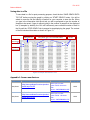
1
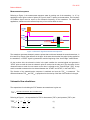
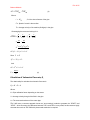
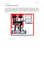
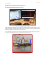
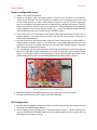
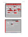
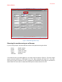
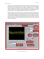
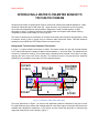
Feb. 2015
Bahram Mirshab
INTERFACING A WATER FLOW-METER SENSOR TO
TDC1000-TDC7200EVM
Ultrasonic flow-meters are gaining wide usage in commercial, industrial and medical applications. Major
benefits of utilizing this type of flow meter are; higher accuracy, low maintenance (no moving parts),
non-invasive flow measurement, and the ability to diagnose the meter’s health regularly. A major
advantage of using TI’s ultrasonic sensing is the ultralow power consumption which allows metering
companies to use the same battery for a very long time.
This article is intended as an introduction to ultrasonic flow sensing and describes demonstration a setup
to measure velocity of flow in a pipe using an ultrasonic water flow-meter sensor, TDC1000 ultrasonic
analog-front-end (UAFE) and TDC7200 precision time interval timer.
Background: Transient-time Ultrasonic Flow-meters
In Figure 1, a typical ultrasonic flow sensor is shown. The sensor consist of a pipe with nominal diameter
of “D” and two piezoelectric transducers placed at fixed distance “L” from each other. The transducers are
mounted in a protective housing. The housing and the transducers are inserted in the holes in the pipe,
exposing the inner cover to the fluid in the pipe. Two reflection mirrors in the pipe direct the ultrasonic
signals from one transducer to the other one in the opposite location.
Figure 1. ultrasonic water flow-meter pipe.
The single path sensor of Figure 1 is used for flow applications where the diameter of the pipe is small.
For larger diameter pipes sensors with multiple paths are used. Other types of ultrasonic flow sensors are
available with clamped-on transducers. In this article we have limited the discussion to reflective-type
single path sensors such as one shown in Figure 1.
Feb. 2015
Bahram Mirshab
Measurement sequence
Referring to Figure 2, the measurement sequence starts by exciting one of the transducer, i.e. “A”, by
applying a burst of given number of pulses (in Figure 2, three TX pulses) to the transducer. The frequency
of excitation signal must be equal to the resonance frequency of the transducer. For water flow
applications, transducers with resonant frequency of one to three MHz are used.
Figure 2. ultrasonic signal measurement sequence.
The transducer generates ultrasonic pressure pulses that are directed towards the second transducer, in
this case B, by means of the reflectors in the pipe. At the same time that the first pulse is being applied to
the transducer, a “START” signal is generated to mark the beginning of the “time-of-flight” measurement.
On the receiver side, the electronic circuits in the path condition the received signal and generate a
“STOP” pulse to mark the time the ultrasonic pulse is received at the other end. The time taken for the
ultrasound wave to travel from one sensor to the other is referred as the “Time-Of-Flight” (TOF). A stop
watch is needed to measure the time internal between the “START” and “STOP”, in this case TOFAB.
The direction of the transmit/receive sequence is switched and next the TOFBA is measured. The
difference between TOFAB and TOFBA is proportional to the velocity of the flow of the medium in the pipe.
Volumetric flow calculations: The expressions for calculating the TOF between two transducers is given as:
TOF =
Referring to Figure 1 , the expressions for TOF for downstream (TOFAB) and upstream (TOFBA) are:
TOFAB=
1
1
L +
TOFBA= L +
+ L
+
L
(1)
(2)
Feb. 2015
Bahram Mirshab
ΔT = TOFBA - TOFAB
(3)
Where:
L =
; D is the inner diameter of the pipe
2
C= Speed of sound in the medium
V= Average velocity of the medium (fluid/gas) in the pipe
Rearranging the terms and solving for V:
ΔTOF= (
+
) -(
+
)
-
=
=
ΔT
= 2 ∗ ∗
Since
≫
~
And
ΔT ∗
= 2 ∗ ∗
∆ ∗
(4)
Calculation of Volumetric Flow rate, Q The relationship for calculate the volumetric flow rate is:
∗
∗
Where:
K = Pipe calibration factor depending on the sensor
V = Average velocity though of the fluid in the pipe.
A = The cross-sectional area of the meter pipe.
TDC 1000 uses a common approach known as “zero-crossing” method to generate the “START” and
“STOP”. At low flow rates, the difference between TOFAB and TOFBA is very small, for this reason a highly
accurate timer such as TDC7200 with picoseconds resolution is required.
Feb. 2015
Bahram Mirshab
Zero Flow Measurement Setup In this document, we describe interfacing of TDC1000 and TDC7200 integrated circuits. The block
diagram of the setup is shown in Figure 3. MSP430 microcontroller is used to programming of TDC1000
and TDC7200 and for communication with a host PC over USB interface. A Graphic User Interface (GUI)
is used for programming the registers of TDC1000 and TDC7200 and for displaying ∆TOF at zero flow
condition.
TDC7200
MSP43XX
Host PC Running TDC1000-7200 GUI
OSC
USB
TDC1000
RREF
A
B
RTD temp sesnor
Flow
Ultrasonic flow sensor
Figure 3. zero flow measurement setup
Feb. 2015
Bahram Mirshab
The Choice of the Ultrasonic Flow-meter Sensor The zero-flow demonstration setup is shown in Figure 4.
Figure 4. zero flow demonstration setup
System requirements, standards, and cost dictate the choice of flow-meter sensors. Water is a good
medium for propagating ultrasonic pressure pulse and the most common sensors in this application have
resonance frequency in the range of MHz, 1 MHz in this case.
For the demonstration purpose we use an Audiowell ultrasonic water flow-meter pipe shown in Figure 4.
This sensor can be obtained from the source included in the reference section.
Figure 5. ultrasonic flow-meter sensor pipe
Feb. 2015
Bahram Mirshab
Steps to configure the setup 1. Obtain a TDC1000-TDC7200EVM
2. Obtain the ultrasonic water flow sensor shown in Figure 5 from the source in the reference
section of this document. The union and the pipe extension are not necessary for zero flow test
but you would need the end caps to confine water in the pipe for the test. The RTD temperature
senor is not include in the sensor and can be obtained from a different manufacturer. The RTD
used in this setup is a JUMO PT1000. If you need to use a PT500 temperature senor, you would
need to change the temp sensor reference resistor (RREF) on the TDC1000-TDC7200EVM to 500
Ω (the EVM board comes with a 1000 Ω resistor reference resistor).
3. Place a cap at one end of the sensor and fill the pipe with clean water. Make sure there are no
bubbles trapped in the sensor. Place the second cap and the open end open of the pipe to
confine water inside the pipe.
4. Connect the sensor to the EVM connector as shown below. Place the pipe on a flat surface in a
standup position as shown if Figure 4. This would move up any bubbles trapped between the two
transducers to the top of the pipe and away from the signal path. Bubbles trapped in the signal
path causes severe attenuation of signal.
5. You may want to view the signal waveforms (Start, Stop, and Ultrasound received waveform at
the input of TDC1000 internal comparators) on a scope to make sure proper operation of the
sensor. You can either connect the scope probes to the provided terminals (test points) on the
EVM or solder SMA connector on the EVM board and use the cables shown in Figure 4
Figure 6, EVM connections to the sensor
6. Install the TDC1000-TDC7200EVM software per the instruction in the user’s manual
7. Connect the EVM to the Host PC using the provided USB cable
GUI Configuration 8. Run the GUI; if prompted, upgrade the version of the EVM firmware per the instructions in the
TDC1000-TDC7200EVM User’s Manual.
9. Set the registers in the TDC1000 menu to the values shown in Figure 7, Figure 8, and Figure 9.
Flip the “CONTINOUS TRIGGER” switch to the top position (switch will turn to green from red
indicating that the system is running).
Feb. 2015
Bahram Mirshab
Divide by 8
8 pulses
1 Cycle
5 STOPS
Enabled
TOF Measurement
Enabled
Disabled
PT1000
Mode 2
-125mV
15 dB
Disabled
Active
Bypass
Single Echo
38
Divided by 1
Figure 7. TDC1000 setup menu in the GUI
Figure 8. Sampling interval setup
Flip to
continuous
trigger position
Feb. 2015
Bahram Mirshab
Figure 9. TDC7200 registers setup
Observing the waveform using an oscilloscope If you are using a scope, use three channels to observe the signal traces as given below:
CHA A :
CHA B:
CHA C:
Trigger:
Time base:
START, 5V/DIV
STOP, 5V/DIV
COMP_IN, 5V/DIV
Normal, on Ch A
20uV/DIV
You should be able to get similar display on you scope screen as shown in Figure 10. The time of flight
can be measured reference to STOP pulse one to five. When calculating the delta TOF, if the same
STOP pulse is used to measure the TOF for upstream and downstream, the net effect is canceled out
and the delta TOF is the same no matter what STOP pulse is used to measure The TOF.
Feb. 2015
Bahram Mirshab
Figure 10. scope trace TOF measurement sequence
Now change the time base of the scope to 200 uV/DIV, you should see the TX/RX sequence for both
directions as shown in Figure 11. In mode 2 of TDC1000 operation if CH_SWP is enabled, the state
machine upon receiving a trigger pulse will TX/RX in one direction, then switch the direction and upon
receiving a second trigger will TX/RX in the other direction.
Figure 11. ∆TOF measurement sequence
Displaying the delta TOF in GUI’s GRAPH menu Click on the “GRAPH” tab to display the “GRAPH” menu. In the box below “Flow MODE” on the
right bottom corner of the display, check the flow mode option. In this mode the GUI generates a
Feb. 2015
Bahram Mirshab
downstream and upstream sequence and calculates the “Delta TOF” and display it at the top right
of the screen under “FLOW DELTA AVG (ns)”. Under “TDC_SELECT” chose the STOP pulse
(STOP1, STOP2, etc) that provides the best accuracy in calculating the TOF. Try different
selection and observe the changes in delta TOF and STADEV. As mentioned in the previous
section, as the TOF in the upstream and the downstream directions are measured reference to
the same STOP pulse, the net effect is independent of the choice of the STOP pulse.
To start the graph, click on “START Graph” tab, you should see the yellow moving trace of the
delta TOF versus time as shown in Figure 12. If the numbers in delta TOF and the STDEV boxes
are changing but the graph is not being displayed (black screen) then the graph is out of scale.
To force the graph to be displayed in the window, place the cursor on the black background and
right-click your mouse. A drop window display will show up giving you the option to select auto
scale in the X and Y axis. Once you check mark the auto scale box, the GUI will scale the graph
to fit in the display window.
Figure 12. ∆TOF graph display
Feb. 2015
Bahram Mirshab
Saving data in a file To save data in a file for post processing purpose, check the box “SAVE GRAPH DATA
TO FILE” before running the graph by clicking on “START GRAPH” button. You will be
asked to name the file and identify a location on your computer to store the file. When
you type in the information click the ok tab, you will be prompted to type the number of
samples to be saved. If type ok without typing in the number of samples in the displayed
box (0 samples by default), the GUI will continuously save unlimited number of data in
the file until the “STOP GRAPH” tab is pressed to stop displaying the graph. The content
of the file includes information as shown in Figure 13.
TOF referenced to
STOP1 pulse (ns)
Delta TOF (nS) based on the STOP pulse selected in the
“TDC_SELECT” box. In this case START-STOP2
= B2 -B3
TOF
downstream
TOF
downstream
Figure 13. Sample data stored in a file
Appendix 1: Sensor manufacturer Application Manufacturer P/N FR (kHz) Heat/water
AudioWell
Brass Pipe For Heat
http://www.audiowell.com/en/productmeter DN25. Ultrasonic
detail.aspx?id=80
flow
sensor AW5Y0980K04L193Z
1000
Heat/water
AudioWell
Brass Pipe For Heat
http://www.audiowell.com/en/productmeter DN20. Ultrasonic
detail.aspx?id=80
flow
sensor AW5Y0980K08L151Z
1000