Download "user manual"

Abteilung Software Engineering
Fakultät II – Informatik, Wirtschafts- und Rechtswissenschaften
Department für Informatik
Diploma Thesis
Workload-sensitive
Timing Behavior Anomaly Detection
in Large Software Systems
André van Hoorn
September 14, 2007
First examiner:
Prof. Dr. Wilhelm Hasselbring
Second examiner: MIT Matthias Rohr
Advisor:
MIT Matthias Rohr
Abstract
Anomaly detection is used for failure detection and diagnosis in large software systems
to reduce repair time, thus increasing availability. A common approach is building a
model of a system’s normal behavior in terms of monitored parameters, and comparing
this model with a dynamically generated model of the respective current behavior. Deviations are considered anomalies, indicating failures. Most anomaly detection approaches
do not explicitly consider varying workload.
Assuming that varying workload leads to varying response times of services provided
by internal software components, our hypothesis is as follows: a novel workload-sensitive
anomaly detection is realizable, using statistics of workload-dependent service response
times as a model of the normal behavior.
The goals of this work are divided into three parts. First, an application-generic technique will be developed to define and generate realistic workload based on an analytical
workload model notation to be specified. Applying this technique to a sample application in a case study, the relation between workload intensity and response times will be
statistically analyzed. Based on this, a workload-sensitive anomaly detection prototype
will be implemented.
iii
Contents
1 Introduction
1.1 Motivation . . . . . . . . . . . . . . . . . . . . . . . . . . . . . . . . . . .
1.2 Goals . . . . . . . . . . . . . . . . . . . . . . . . . . . . . . . . . . . . . .
1.3 Document Structure . . . . . . . . . . . . . . . . . . . . . . . . . . . . .
2 Foundations
2.1 System Model . . . . . . . . . . . . . . . .
2.2 Performance Metrics and Scalability . . . .
2.3 Workload Characterization and Generation
2.4 Probability and Statistics . . . . . . . . .
2.5 Anomaly Detection . . . . . . . . . . . . .
2.6 Apache JMeter . . . . . . . . . . . . . . .
2.7 JPetStore Sample Application . . . . . . .
2.8 Tpmon . . . . . . . . . . . . . . . . . . . .
2.9 Related Work . . . . . . . . . . . . . . . .
.
.
.
.
.
.
.
.
.
.
.
.
.
.
.
.
.
.
.
.
.
.
.
.
.
.
.
.
.
.
.
.
.
.
.
.
.
.
.
.
.
.
.
.
.
3 Probabilistic Workload Driver
3.1 Requirements Definition . . . . . . . . . . . . . . .
3.1.1 Requirements Labeling and Classification . .
3.1.2 Assumptions . . . . . . . . . . . . . . . . . .
3.1.3 Supported Applications . . . . . . . . . . . .
3.1.4 Use Cases . . . . . . . . . . . . . . . . . . .
3.1.5 Workload Configuration . . . . . . . . . . .
3.1.6 User Interface . . . . . . . . . . . . . . . . .
3.2 Design . . . . . . . . . . . . . . . . . . . . . . . . .
3.2.1 System Model . . . . . . . . . . . . . . . . .
3.2.2 Workload Configuration Data Model . . . .
3.2.3 Architecture and Iterative Execution Model
3.3 Markov4JMeter . . . . . . . . . . . . . . . . . . . .
3.3.1 Test Elements . . . . . . . . . . . . . . . . .
3.3.2 Behavior Files . . . . . . . . . . . . . . . . .
3.3.3 Behavior Mix Controller . . . . . . . . . . .
3.3.4 Session Arrival Controller . . . . . . . . . .
3.4 Using Markov4JMeter . . . . . . . . . . . . . . . .
.
.
.
.
.
.
.
.
.
.
.
.
.
.
.
.
.
.
.
.
.
.
.
.
.
.
.
.
.
.
.
.
.
.
.
.
.
.
.
.
.
.
.
.
.
.
.
.
.
.
.
.
.
.
.
.
.
.
.
.
.
.
.
.
.
.
.
.
.
.
.
.
.
.
.
.
.
.
.
.
.
.
.
.
.
.
.
.
.
.
.
.
.
.
.
.
.
.
.
.
.
.
.
.
.
.
.
.
.
.
.
.
.
.
.
.
.
.
.
.
.
.
.
.
.
.
.
.
.
.
.
.
.
.
.
.
.
.
.
.
.
.
.
.
.
.
.
.
.
.
.
.
.
.
.
.
.
.
.
.
.
.
.
.
.
.
.
.
.
.
.
.
.
.
.
.
.
.
.
.
.
.
.
.
.
.
.
.
.
.
.
.
.
.
.
.
.
.
.
.
.
.
.
.
.
.
.
.
.
.
.
.
.
.
.
.
.
.
.
.
.
.
.
.
.
.
.
.
.
.
.
.
.
.
.
.
.
.
.
.
.
.
.
.
.
.
.
.
.
.
.
.
.
.
.
.
.
.
.
.
.
.
.
.
.
.
.
.
.
.
.
.
.
.
.
.
.
.
.
.
.
.
.
.
.
.
1
1
2
3
.
.
.
.
.
.
.
.
.
5
5
7
9
13
18
20
22
23
26
.
.
.
.
.
.
.
.
.
.
.
.
.
.
.
.
.
29
29
29
30
30
31
32
33
33
34
34
37
39
40
41
42
42
42
v
Contents
4 Experiment Design
4.1 Markov4JMeter Profile for JPetStore . . . . . . . .
4.1.1 Identification of Services and Request Types
4.1.2 Application Model . . . . . . . . . . . . . .
4.1.3 Behavior Models . . . . . . . . . . . . . . .
4.1.4 Probabilistic JMeter Test Plan . . . . . . .
4.2 Configuration . . . . . . . . . . . . . . . . . . . . .
4.2.1 Node Configuration . . . . . . . . . . . . . .
4.2.2 Monitoring Infrastructure . . . . . . . . . .
4.2.3 Adjustment of Default Software Settings . .
4.2.4 Definition of Experiment Runs . . . . . . . .
4.3 Instrumentation . . . . . . . . . . . . . . . . . . . .
4.3.1 Assessment of Monitoring Overhead . . . . .
4.3.2 Identification of Monitoring Points . . . . .
4.4 Workload Intensity Metric . . . . . . . . . . . . . .
4.4.1 Formal Definition . . . . . . . . . . . . . . .
4.4.2 Implementation . . . . . . . . . . . . . . . .
4.5 Execution Methodology . . . . . . . . . . . . . . .
.
.
.
.
.
.
.
.
.
.
.
.
.
.
.
.
.
.
.
.
.
.
.
.
.
.
.
.
.
.
.
.
.
.
.
.
.
.
.
.
.
.
.
.
.
.
.
.
.
.
.
.
.
.
.
.
.
.
.
.
.
.
.
.
.
.
.
.
.
.
.
.
.
.
.
.
.
.
.
.
.
.
.
.
.
.
.
.
.
.
.
.
.
.
.
.
.
.
.
.
.
.
.
.
.
.
.
.
.
.
.
.
.
.
.
.
.
.
.
.
.
.
.
.
.
.
.
.
.
.
.
.
.
.
.
.
.
.
.
.
.
.
.
.
.
.
.
.
.
.
.
.
.
.
.
.
.
.
.
.
.
.
.
.
.
.
.
.
.
.
.
.
.
.
.
.
.
.
.
.
.
.
.
.
.
.
.
.
.
.
.
.
.
.
.
.
.
.
.
.
.
.
.
.
47
47
47
48
49
50
53
53
53
54
55
56
56
57
59
59
60
61
5 Analysis
5.1 Methodology . . . . . . . . . . . . . . . . . . .
5.1.1 Transformations of Raw Data . . . . . .
5.1.2 Visualization . . . . . . . . . . . . . . .
5.1.3 Examining and Extracting Sample Data
5.1.4 Considered Statistics . . . . . . . . . . .
5.1.5 Parametric Density Estimation . . . . .
5.2 Data Description . . . . . . . . . . . . . . . . .
5.2.1 Platform Workload Intensity . . . . . . .
5.2.2 Throughput . . . . . . . . . . . . . . . .
5.2.3 Descriptive Statistics . . . . . . . . . . .
5.2.4 Distribution Characteristics . . . . . . .
5.2.5 Distribution Fitting . . . . . . . . . . . .
5.3 Summary and Discussion of Results . . . . . . .
.
.
.
.
.
.
.
.
.
.
.
.
.
.
.
.
.
.
.
.
.
.
.
.
.
.
.
.
.
.
.
.
.
.
.
.
.
.
.
.
.
.
.
.
.
.
.
.
.
.
.
.
.
.
.
.
.
.
.
.
.
.
.
.
.
.
.
.
.
.
.
.
.
.
.
.
.
.
.
.
.
.
.
.
.
.
.
.
.
.
.
.
.
.
.
.
.
.
.
.
.
.
.
.
.
.
.
.
.
.
.
.
.
.
.
.
.
.
.
.
.
.
.
.
.
.
.
.
.
.
.
.
.
.
.
.
.
.
.
.
.
.
.
.
.
.
.
.
.
.
.
.
.
.
.
.
65
65
65
66
67
69
69
70
70
70
71
79
81
83
6 Workload-Intensity-sensitive Anomaly Detection
6.1 Anomaly Detection in Software Timing Behavior . . . . . . . . . . . . .
6.2 Plain Anomaly Detector . . . . . . . . . . . . . . . . . . . . . . . . . . .
6.3 Workload-Intensity-sensitive Anomaly Detector . . . . . . . . . . . . . .
85
85
85
87
7 Conclusion
7.1 Summary . . . . . . . . . . . . . . . . . . . . . . . . . . . . . . . . . . .
7.2 Discussion . . . . . . . . . . . . . . . . . . . . . . . . . . . . . . . . . . .
7.3 Future Work . . . . . . . . . . . . . . . . . . . . . . . . . . . . . . . . . .
89
89
91
92
vi
.
.
.
.
.
.
.
.
.
.
.
.
.
.
.
.
.
.
.
.
.
.
.
.
.
.
Contents
A Workload Driver
A.1 Available JMeter Test Elements . . . . . . . . . . . . . . . . . . . . . . .
A.2 Installing Markov4JMeter . . . . . . . . . . . . . . . . . . . . . . . . . .
B Case Study
B.1 Installation Instructions for Instrumented JPetStore
B.1.1 Install and Configure Apache Tomcat . . . .
B.1.2 Build and Install JPetStore . . . . . . . . .
B.1.3 Monitor JPetStore with Tpmon . . . . . . .
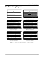
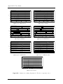
B.2 Trace Timing Diagrams . . . . . . . . . . . . . . .
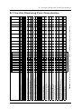
B.3 Iterative Monitoring Point Determination . . . . . .
.
.
.
.
.
.
.
.
.
.
.
.
.
.
.
.
.
.
.
.
.
.
.
.
.
.
.
.
.
.
.
.
.
.
.
.
.
.
.
.
.
.
.
.
.
.
.
.
.
.
.
.
.
.
.
.
.
.
.
.
.
.
.
.
.
.
.
.
.
.
.
.
95
95
96
97
97
97
98
99
101
103
Acknowledgement
105
Declaration
107
Bibliography
109
vii
List of Figures
2.1
2.2
2.3
2.4
2.5
2.6
2.7
2.8
2.9
2.10
2.11
2.12
2.13
2.14
2.15
2.16
2.17
2.18
Example HTTP communication . . . . . . . . . . . . . . . . . . . . .
Sequence diagram showing a sample trace . . . . . . . . . . . . . . .
Efficiency in the ISO 9126 standard . . . . . . . . . . . . . . . . . . .
Timing metrics on system- and on application-level . . . . . . . . . .
Impact of increasing workload on throughput and end-to-end response
Hierarchical workload model . . . . . . . . . . . . . . . . . . . . . . .
Example Costumer Behavior Model Graph . . . . . . . . . . . . . . .
Example Extended Finite State Machine . . . . . . . . . . . . . . . .
Workload generation approach . . . . . . . . . . . . . . . . . . . . . .
Graphs of density functions for normal and log-normal distributions .
Description of a box-and-whisker plot . . . . . . . . . . . . . . . . . .
Kernel density estimations of a data sample . . . . . . . . . . . . . .
Chain of dependability threats . . . . . . . . . . . . . . . . . . . . . .
JMeter GUI . . . . . . . . . . . . . . . . . . . . . . . . . . . . . . . .
JMeter Architecture. . . . . . . . . . . . . . . . . . . . . . . . . . . .
JPetStore index page . . . . . . . . . . . . . . . . . . . . . . . . . . .
Instrumented system and weaving of an annotated operation . . . . .
Aspect weaver weaves aspects and functional parts into single binary
. .
. .
. .
. .
time
. .
. .
. .
. .
. .
. .
. .
. .
. .
. .
. .
. .
. .
6
7
7
8
9
10
11
12
13
15
16
17
18
20
21
22
24
24
3.1
3.2
3.3
30
34
3.4
3.5
3.6
3.7
3.8
3.9
3.10
3.11
3.12
3.13
3.14
3.15
Use cases of the workload driver . . . . . . . . . . . . . . . . . . . . . . .
Class diagram of the workload configuration data model . . . . . . . . .
Sample application model illustrating the separation into session layer and
protocol layer . . . . . . . . . . . . . . . . . . . . . . . . . . . . . . . . .
Transition diagrams of two user behavior models . . . . . . . . . . . . . .
Architecture overview of workload driver in UML class diagram notation
Sketch of algorithm executed by a user simulation thread executing a session
Integration of Markov4JMeter into the JMeter architecture . . . . . . . .
Probabilistic Test Plan and Markov4JMeter configuration dialogs . . . .
User behavior model stored in CSV file format . . . . . . . . . . . . . . .
Prepared JMeter Test Plan . . . . . . . . . . . . . . . . . . . . . . . . . .
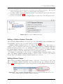
New entries in context menu . . . . . . . . . . . . . . . . . . . . . . . . .
Markov4JMeter Test Plan . . . . . . . . . . . . . . . . . . . . . . . . . .
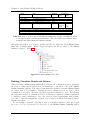
Example Behavior Mix. . . . . . . . . . . . . . . . . . . . . . . . . . . . .
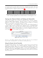
Example BeanShell script defining number of active sessions . . . . . . .
Using a BeanShell script within the Session Arrival Controller . . . . . .
4.1
Session layer and two protocol states of JPetStore’s application model . .
49
35
36
37
38
40
41
42
43
43
44
45
46
46
ix
List of Figures
4.2
4.3
4.4
4.5
4.6
4.7
4.8
Transition graphs of browsers and buyers . . . . . . . . . . . . . . .
Probabilistic Test Plan and configuration of state View Cart . . . .
Access log entry of HTTP requests for JPetStore . . . . . . . . . .
Graphs of monitored resource utilization data from server and client
Sample trace timing diagrams for a request . . . . . . . . . . . . . .
Platform workload intensity graphs . . . . . . . . . . . . . . . . . .
Sketch of experiment execution script . . . . . . . . . . . . . . . . .
. . .
. . .
. . .
node
. . .
. . .
. . .
50
51
54
54
58
60
62
5.1
5.2
5.3
5.4
5.5
5.6
5.7
5.8
5.9
5.10
66
68
69
70
71
71
73
74
75
5.11
5.12
5.13
5.14
5.15
5.16
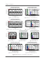
Overview of all plot types used . . . . . . . . . . . . . . . . . . . . . . .
Differences in sample data for both Tpmon modes . . . . . . . . . . . . .
Scatter plot and box-and-whisker plot showing ramp-up time . . . . . . .
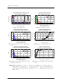
Number of users vs. platform workload intensity . . . . . . . . . . . . . .
Number of users vs. throughput . . . . . . . . . . . . . . . . . . . . . . .
Number of users vs. minimum response times . . . . . . . . . . . . . . .
Platform workload intensity vs. maximum response times . . . . . . . . .
Platform workload intensity vs. stretch factors of mean, median, and mode
Platform workload intensity vs. 1. quartile response times . . . . . . . .
Platform workload intensity vs. means, medians, modes of response times
and quartile stretch factors . . . . . . . . . . . . . . . . . . . . . . . . . .
Platform workload intensity vs. 3. quartile response times . . . . . . . .
Platform workload intensity vs. variance, standard deviation, and skewness.
Platform workload intensity vs. outlier ratios . . . . . . . . . . . . . . . .
Examples for all identified density shapes . . . . . . . . . . . . . . . . . .
Goodness of fit visualizations for an operation . . . . . . . . . . . . . . .
Box-and-whisker plot for varying workload intensity . . . . . . . . . . . .
6.1
6.2
6.3
Anomaly detection scenario with constant workload intensity (PAD) . . .
Anomaly detection scenario with increasing workload intensity (PAD) . .
Anomaly detection scenario with increasing workload intensity (WISAD)
86
87
88
A.1 New entries in context menu . . . . . . . . . . . . . . . . . . . . . . . . .
96
76
77
78
79
80
82
83
B.1 Sample trace timing diagrams for JPetStore requests. . . . . . . . . . . . 101
B.1 Sample trace timing diagrams for JPetStore requests (cont.). . . . . . . . 102
x
List of Tables
2.1
Mean and variance for discrete and continuous probability distributions .
14
3.4
3.5
Configuration of HTTP Request Samplers . . . . . . . . . . . . . . . . .
Configuration of guards and actions . . . . . . . . . . . . . . . . . . . . .
44
45
4.1
4.2
4.3
4.4
4.5
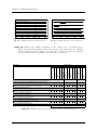
Identified service and request types of JPetStore . . . . . . . . .
Overview of varying parameters for all experiments. . . . . . . .
Response time statistics with different monitoring configurations
Identified monitoring points and coverage of request types . . .
Table description of JPetStore database schema . . . . . . . . .
.
.
.
.
.
48
56
57
58
62
A.1 Available JMeter Test Elements . . . . . . . . . . . . . . . . . . . . . . .
95
.
.
.
.
.
.
.
.
.
.
.
.
.
.
.
.
.
.
.
.
B.1 Response time statistics and request coverage of JPetStore operations . . 103
xi
Chapter 1
Introduction
1.1 Motivation
Today’s enterprise applications are large-scale multi-tiered software systems involving
Web servers, application servers and database servers. Examples are banking and online
shopping systems or auction sites. Especially if these systems are accessible through
the Internet and thus exposed to unpredictable workload, they must be highly scalable.
The availability of such systems is a critical requirement since operational outages are
cost-intensive.
Anomaly detection is used for failure detection and diagnosis not only in large software
systems. A common approach for detecting anomalies is building a model of a system’s
“normal behavior” in terms of monitored parameters, and comparing this model with
the respective current behavior to uncover deviations. The data being monitored can
be obtained from different levels, e.g. network-, hardware-, or application-level. Failures
may be detected proactively but at least quickly after they occur. Repair times can be
reduced, by taking appropriate steps immediately, thus increasing availability.
Timing behavior anomaly detection approaches exist which are based on monitored
component response times on application-level. However, most of them do not explicitly
consider that a varying workload intensity leads to varying response times. For example,
when using preset threshold values, this often leads to spurious events when the workload
intensity increases.
This work targets on a timing behavior anomaly detection which explicitly considers
this additional parameter. For this purpose, we statistically analyze the relation between
workload intensity and response times in a case study. A workload driver is developed
which generates varying workload based on probabilistic models of user behavior. The
results of the analysis are used for a workload-intensity-sensitive anomaly detection prototype but they are interesting for timing behavior evaluation of multi-user systems in
general.
The goals of our work are presented in the following Section 1.2. An overview of the
document structure is given in Section 1.3.
1
Chapter 1 Introduction
1.2 Goals
Our work is divided into the three parts covering workload generation, component
response time analysis in a case study, and developing an anomaly detection protype
based on the findings from the analysis part. These three parts are outlined in the
following paragraphs.
Workload Driver
To systematically obtain workload-dependent performance data from Web-based applications, workload is usually generated synthetically by executing a number of threads
emulating users accessing the application under test. A common approach is to replicate
a number of pre-recorded traces to multiple executing threads. Tools exist which allow for
capturing and replaying those traces. A major drawback of this approach comes with the
fact that only a limited number of traces is executed, instead of dynamically generating
valid traces which cover the application in a more realistic manner. In our case we need
such realistic workload since we want to obtain response time data of all components and
thus, the application functionality must be covered much more thoroughly.
We aim at developing a technique which leads to more realistic workload than this is
the case with the classical capture-and-replay approach. The intended procedure is as
follows. First, the possible usage sequences are modeled for an application. This model
may be enriched with probabilities to weigh possible usage alternatives. Based on this
model, valid traces are generated and a configurable number of users is emulated.
Case Study
In a case study, workload-dependent distributions of service response times shall be
obtained from an existing Web-based application. The functionality to measure the
response times is considered to be given. First, our developed workload generation approach needs to be applied to this specific application. Moreover, its appropriateness
has to be evaluated. A large number of experiments must be executed, exposing the
application to varying workload. The obtained response time data has to be processed
by a statistical processing and graphics tool such as the GNU R Environment (R Development Core Team, 2005). The results have to be analyzed to derive characteristics of the
response time distributions with respect to the varying workload. For example we are
interested in the similarity of the response times when workload varies. Mathematical
probability density functions containing the workload parameter as a third dimension
shall be determined, approximating these distributions.
The Java BluePrints group (Sun Microsystems, Inc., 2007) provides the Java Pet Store
J2EE reference application (Sun Microsystems, Inc., 2006) which is intended to be used
in our case study. It is the sample application presented in (Singh et al., 2002) and used
in literature, e.g. by Chen et al. (2005), Kiciman and Fox (2005). The Java Pet Store
has been extended by the above-mentioned monitoring functionality already. First, the
application’s stability in terms of long periods of high workload needs to be evaluated.
Alternative applications which may be used in case our Pet Store stability evaluation
2
1.3 Document Structure
fails, are the TPC-W online bookstore (Transaction Processing Performance Council,
2004) and RUBiS (ObjectWeb Consortium, 2005) which models an online auction site.
Both applications are available in J2EE implementation variants and are also commonly
used in literature, e.g. by Amza et al. (2002), Cecchet et al. (2002), Agarwal et al. (2004),
and Pugh and Spacco (2004).
Workload-sensitive Anomaly Detection Prototype
Based on the relations between workload intensity and response times derived in the
analysis part of the case study, a prototype of a workload-sensitive anomaly detection
shall be implemented. A degree of anomaly for service call response times shall be
computed and the prototype shall provide simple visualization functionality.
1.3 Document Structure
This document is structured as follows.
• Chapter 2 contains the foundations of our work. Starting with a description of the
considered system model, an introduction into performance metrics and scalability,
workload characterization and generation for Web-based system, probability and
statistics as well as anomaly detection follows. Moreover, we describe the software
we used and present related work.
• Chapter 3 deals with the probabilistic workload driver. Based on a requirements
definition, the design of the workload driver is described. The implementation
called Markov4JMeter is outlined and an example of use is presented.
• Chapter 4 contains the description of the experiment design. A probabilistic workload driver profile for the sample application JPetStore, according to the design in
Chapter 3, is created. Appropriate monitoring points have been determined and a
workload intensity metric is defined. Moreover, the configuration of the machines,
the software, and the experiment runs is described.
• Chapter 5 deals with the statistical analysis of the data obtained in the experiments.
After outlining the analysis methodology, we give a detailed description of the
results and conclude with a summary and discussion of these.
• Based on the results of Chapter 5, a workload-intensity-sensitive anomaly detection
prototype has been developed. This is part of Chapter 6.
• Chapter 7 contains the conclusion of our work including a summary, a discussion,
and the presentation of future work.
• The Appendix contains additional resources which are referenced by the related
chapters of this document.
3
Chapter 2
Foundations
This chapter contains the foundations of our work. In Section 2.1 we describe the considered system model. An introduction into performance metrics and scalability is given
in Section 2.2. Section 2.3 deals with workload characterization and generation for Webbased system. An introduction into the theory of probability and statistics, as far as
this is relevant for our work, is presented in Section 2.4. Section 2.5 outlines the concept
of anomaly detection and presents existing approaches. The workload driver JMeter,
our probabilistic workload driver presented in Chapter 3 is based on, is described in
Section 2.6. Sections 2.7 and 2.8 present the JPetStore sample application and the monitoring infrastructure Tpmon which are both used in the case study. Section 2.9 gives an
overview about related work.
2.1 System Model
This section gives an overview of the system model used throughout this document. It
contains a description of an enterprise information system, the HTTP request/response
model used by those systems as well as the considered execution model and related terms.
Enterprise Information Systems
Enterprise information systems (EIS) are large software systems, e.g. banking and online
shopping systems or auction sites. Usually they are component-based and multi-tiered,
i.e. they consist of a Web Server, an application server and a database server (Menascé
and Almeida, 2000).
The Web server executes an HTTP server software listening for incoming HTTP requests (see section below), establishing the required connection between itself and the
client, sending the requested response, and returning to its listening functionality. An application server runs the enterprise software that processes all services provided through
the Web server. The database server executes a database management system (DBMS)
holding the persistent data accessed by the application.
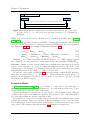
HTTP Request/Response Model
The Hypertext Transfer Protocol (HTTP) is a request/response protocol. An HTTP
communication is initiated by an HTTP request issued by a client and results in an
5
Chapter 2 Foundations
SQD HTTP Communication
http client
http server
commhttp ("GET", "foo.com/news.shtml?id=12", <Accept−Charset="ISO−8859−1,utf−8",...>, <>)
("OK", <Content−Type="text/html",...>, <"<html>...</html>">)
Figure 2.1: Example HTTP communication. A client requests the resource /news.shtml
from the server foo.com. The server responds with a message body containing an
HTML file.
HTTP response from the server. Details can be obtained from RFC 2616 (Fielding
et al., 1999).
We model the relevant elements of an HTTP communication by means of the function
commhttp : an HTTP request req ∈ Reqhttp results in an HTTP response resp ∈ Resphttp
(see Equations 2.1–2.3). An example is illustrated in Figure 2.1.
commhttp : Reqhttp 7→ Resphttp
Reqhttp : = Methodhttp × URIhttp × Headerhttp × Bodyhttp
Resphttp : = Statushttp × Headerhttp × Bodyhttp
(2.1)
(2.2)
(2.3)
Methodhttp is a string describing the HTTP method, e.g. “GET“ simply requests
the content of a resource referred to by the Uniform Resource Identifier (URI) URIhttp .
Headerhttp simply as a list of name-value pairs containing meta-information about the
request or the response, e.g. a set of content encodings accepted by the client or the
content type of the message body Bodyhttp sent by the server. Statushttp is a string
indicating the status of the result, e.g. ”OK“ or “Not Found”.
We give the ordered tuple as in Figure 2.1 when referencing complete HTTP messages,
using left and right braces h, i to denote lists. When referencing specific fields of a
message, we use an indexed notation, e.g. resp.body or resp.status to get the body and
the status of an HTTP response.
Execution Model
As Menascé and Almeida (2000), we consider a component a “modular unit of
functionality, accessed through defined interfaces”. A component provides a set of operations which can be called by other components.
Operation calls may be synchronous or asynchronous. When synchronously calling an
operation, the caller blocks until the operation has executed. The caller immediately
proceeds when calling an operation asynchronously.
We consider a trace a record of synchronous operation calls of an application processing
a single user request. Traces are assigned a unique identifier. Active traces are those
traces currently processed by the system. Possible starts of a trace are denoted application
entry points. The sequence diagram in Figure 2.2 illustrates a sample trace.
6
2.2 Performance Metrics and Scalability
SQD Sample Trace
a
c
b
a()
b()
c()
c()
Figure 2.2: Sequence diagram showing a sample trace. Component a calls the operation
b() twice. While executing b() the first time, operation c() is called synchronously.
Operation a() is the application entry point.
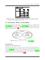
2.2 Performance Metrics and Scalability
Performance denotes the time behavior and resource efficiency of a computer system
(Kozoliek, 2007). The ISO 9126 standard (ISO/IEC, 2001) contains a definition of the
term efficiency with an analogous meaning. It consists of time behavior and resource
utilization metrics (see Figure 2.3). The following sections introduce the metrics used
throughout this document.
Efficiency
Time
Behavior
Resource
Utilization
Response Time,
Throughput,
Reaction Time,
...
CPU Utilization,
Memory Utilization,
I/O Utilization,
...
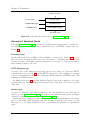
Figure 2.3: Efficiency in the ISO 9126 standard (Kozoliek, 2007).
Time Behavior
Response Time and Execution Time
On system-level, the (end-to-end) response time denotes the time interval elapsed between a request is issued by a user and the time the system answers with an according
response (Jain, 1991). Depending on the measurement objective, the time interval ends
with the system starting to serve its response or the response completion. Jain (1991)
considers this as the “realistic request and response” since the duration of the response
transmission is taken into account (see Figure 2.4(a)).
7
Chapter 2 Foundations
user
user
starts finishes
request request
system
starts
execution
system
starts
response
system
completes
response
user
starts
next
request
b
a
a()
Think Time
Execution Time
=
Response Time
Reaction Time
Execution Time
Time
Response Time
b()
Response Time (1)
Response Time (2)
(a) Both end-to-end response time definitions and
related timing metrics (Jain, 1991).
(b) Operation response and execution
times.
Figure 2.4: Timing metrics on system- and on application-level.
On application-level, response times can be related to operation calls. In this case
the response time is the time interval between the start and the end of an operation
execution. A second metric is the operation’s execution time which is its response time
minus the response times of other operations called in between. Figure 2.4(b) illustrates
both operation call metrics in a sequence diagram.
Throughput
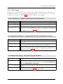
Throughput is the rate at which a system or a system resource handles tasks. The
maximum throughput a system can achieve is referred to as its capacity (Jain, 1991).
The respective unit depends on the system and the measurement objective. For example, the throughput of a Web server may be expressed by the number of requests served
per second. The throughput of a network device can be expressed by the transmitted
data volume per time unit.
Think Time and Reaction Time
The time interval elapsed between two subsequent requests issued by the same user
is called the think time. This can be divided into client-side and server-side think time
depending on from which perspective the measurement takes place (Menascé et al., 1999).
The time interval between a user finishes a request and the system starts its execution
is denoted as the reaction time. Both metrics are included in Figure 2.4(a) (Jain, 1991).
Resource Utilization
The utilization of a system resource is the fraction of time this resource is busy (Jain,
1991). System bottlenecks can be uncovered by monitoring resources with respect to this
metric. For example, the response time of a system may considerably decreases due to a
fully utilized CPU or because the free memory has exceeded.
8
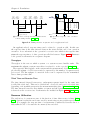
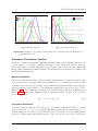
2.3 Workload Characterization and Generation
Throughput
Response Time
Nominal Capacity
Usable
Capacity
Knee Capacity
Workload
Workload
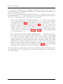
Figure 2.5: Impact of increasing workload on throughput and end-to-end response time
(based on Jain (1991).
Workload and Scalability
The term workload refers to the amount of work that is currently requested from or processed by a system. It is defined by workload intensity and service demand characteristics
(Kozoliek, 2007).
• Workload intensity includes the number of current requests mainly based on the
current number of users and the think times between the requests.
• Service demand characteristics include resource usage on server-side required to
service the requests.
Increasing workload generally implies a higher resource utilization which leads to decreasing performance. The stretch factor is a measure of performance degradation. It is
defined by the ratio of the response time at a particular workload and the response time
at the minimum load.
The term scalability is used to relate to “the ability of a system to continue to meet
its response time or throughput objectives as the demand for the software functions
[workload] increases” (Smith and William, 2001).
Figure 2.5 illustrates the characteristic impact of workload on throughput and response
time. The knee capacity denotes the point until which the throughput increases as the
workload does while having only a small impact on the response time. Until the usable
capacity is reached, response time raises considerably while there’s only little gain for the
throughput. With workload continuing to increase, the throughput may even decrease.
The nominal capacity denotes the maximum achievable throughput under ideal workload
conditions (Jain, 1991).
2.3 Workload Characterization and Generation
This Section gives an overview about how synthetic workload for Web-based systems can
be generated based on models of user behavior. First, a hierarchical workload model
and basic terms for Web-based systems are presented. Examples on how to model user
behavior and how to generate synthetic workload follow.
9
Chapter 2 Foundations
Business Level
3. User Level
2. Application Level
1. Protocol Level
Session Layer
Functional Layer
HTTP Request Layer
Resource Level
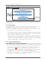
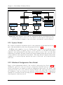
Figure 2.6: A hierarchical workload model (Menascé et al., 2000).
Hierarchical Workload Model
Following Menascé et al. (2000), workload for Web-based systems can be considered to
concern the three layers session layer, functional layer, and HTTP request layer (see
Figure 2.6).
Functional Layer
On the functional layer, an EIS provides a number of services (see Section 2.1), e.g. a
user can browse through product categories, add items to a shopping cart and order its
content. A service call usually requires parameters to be passed, e.g. a product identifier
when adding an item to the cart.
HTTP Request Layer
A service call on the functional layer may involve more than one lower-level HTTP
communications (see Section 2.1) on the HTTP request layer. For example, for creating
a user account it might be necessary to send and confirm a number of HTML forms, each
requiring an HTTP request.
As defined in Section 2.2, the time interval elapsed between the completion of a server
response related to the last request and the invocation of the next one is denoted as the
think time.
Session Layer
A series of consecutive and related requests to the system issued by the same user is
called a session (Menascé et al., 1999). A session starts with the first request and times
out after a certain period of inactivity (Arlitt et al., 2001).
Each sessions has a unique identifier and is associated with state information about the
user, e.g. the items in the shopping cart. The identifier is passed to the server on each
interaction, e.g. by using client-side cookies or by passing the identifier as a paramater
value.
10
2.3 Workload Characterization and Generation
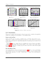
0.4
Exit
0.05
0.2
Browse
0.425
0.05
0.5
Exit
0.35
0.05
0.2
Entry
Exit
0.1
0.2
Add
Select
0.05
0.2
0.5
0.3
Pay
0.35
1
Exit
0.425
Search
0.2
0.05
0.4
Exit
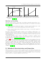
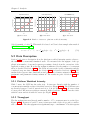
Figure 2.7: Costumer Behavior Model Graph (Menascé et al., 1999).
Modeling User Behavior
Synthetic user sessions may be based upon captured real traces or on analytic workload
models (Barford and Crovella, 1998). Primarily in research papers, workload generators
are presented which base upon mathematical workload models such as Markov chains or
queued networks. In this section we will present two approaches by Menascé et al. (1999)
and Shams et al. (2006).
Costumer Behavior Model Graphs
A (first order) Markov chain is a probabilistic finite state machine with a dedicated entry
and a dedicated exit state. Each transition is weighted with a probability. The sum
of probabilities of outgoing transitions of a state must be 1. Given the current state,
the next state is randomly selected solely based on the probabilities associated with the
outgoing transitions which are stored in a transition matrix.
Menascé et al. (1999) defined a Customer Behavior Model Graph (CBMG) to formally
model the user behavior in Web-based systems using a Markov chain. A CBMG is a pair
(P, Z) of n × n matrices, containing n nodes (states) representing the available requests
a user can issue through the system interface. The matrix P = [pi,j ] represents the
transition probabilities between the states and Z = [zi,j ] represents the average (serverside) think time.
A single CBMG represents the behavior of a class of users, e.g. “heavy buyers”, in
terms of the requests issued within a session. Menascé et al. present an algorithm how
to obtain a desired number of CBMGs from Web log files by means of filtering and
clustering techniques. A state transition Graph for an example CBMG including its
transition probabilities is shown in Figure 2.7.
11
Chapter 2 Foundations
S0
Sign in
A: signed_on=True
Home
S1
S7
Browse
Purchase
Browse
Checkout
P: items_in_cart>0
Delete
A: items_in_cart-=1
P: items_in_cart>0
Browse
S2
Browse
Add
A: items_in_cart+=1
S3
Delete
A: items_in_cart-=1
P: items_in_cart>0
S4
Sign in
A: signed_on=True
S5
Checkout
P: items_in_cart>0
Exit
S6
Exit
S8
Purchase
P: signed_on=True
Exit
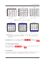
Figure 2.8: Extended Finite State Machine for an online shopping store (following Shams
et al. (2006)).
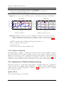
Extended Finite State Machines
Shams et al. (2006) state that CBMGs are inappropriate for modeling valid users sessions.
CBMG are supposed to allow invalid sequences of requests (inter-request dependencies)
and do not provide means for dynamically setting parameter values to be passed with a
request (data dependencies). Shams et al. use Extended Finite State Machines (EFSM)
to model valid application usage. Like a CBMG, an application’s EFSM consists of
different states modeling the request types as well as allowed transitions between them.
Transitions are labeled with predicates and actions. A transition can only be taken if its
associated predicate evaluates to true. When a transition is taken, the respective action
is performed. An EFSM contains a set of variables which can be used in predicate and
action expressions. Values of request parameters are set in actions. A select operation is
provided for assigning values dynamically on trace execution for those values which are
not known before the response of the former request has been received. For example by
means of Browse.Item_ID=select(), the item to browse is chosen dynamically from the
former response. An example EFSM following (Shams et al., 2006) is shown in Figure 2.8.
Workload Generation
Many freely available and commercial Web workload generators exist which provide
functionality to record and replay traces, e.g. Mercury LoadRunner (Mercury Interactive Corporation, 2007), OpenSTA (OpenSTA, 2005), Siege (Fulmer, 2006), and Apache
JMeter (Apache Software Foundation, 2007b) (see Section 2.6). Moreover, sample applications, e.g. TPC-W (Transaction Processing Performance Council, 2004) and RUBiS
(Pugh and Spacco, 2004), exist for benchmarking Web or application servers. They
include functionality to generate workload for the respective application.
12
2.4 Probability and Statistics
Workload Model
Application Model
Sequence Generator
Trace of Sessionlets
SWAT
Trace Generator
Synthetic Workload
Request Generator
System under Study
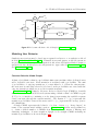
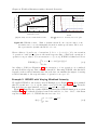
Figure 2.9: Workload generation approach by Shams et al. (2006).
Synthetic workload is usually based on generated user sessions. The included requests
are then executed by a number of threads each representing a virtual user (Ballocca
et al., 2002). We consider the combination of the number of active sessions and the think
times the means to imply the workload intensity. The service demand characteristics are
related to the services called within a session.
Menascé et al. (1999) simulated users whose behavior was derived from CBMGs. Ballocca et al. (2002) propose an integration between existing benchmarking tools and the
CBMG workload characterization model. According to the algorithm by Menascé et al.,
Ballocca et al. derived CBMGs from Web logs. To emulate user behavior matching a
class described by a certain CBMG, they first chose the respective CBMG, selected a
session and then generated a script executing the session reconstructed from the original
session from the Web log. The scripts were executed by the Web stressing tool OpenSTA.
Based on an EFSM capturing inter-request- and data-dependencies, a sequence generator produces a set of sessionlets. A single sessionlet is a valid sequence of request types
representing a session. The stress-testing tool SWAT generates and executes the synthetic
workload based on the set of sessionlets as well additional workload information such as
think time and session length distributions. The approach is illustrated in Figure 2.9
(Shams et al., 2006).
2.4 Probability and Statistics
This section gives an introduction into the theory of probability and statistics as far as
this is relevant for this thesis. Most of the definitions follow Montgomery and Runger
(2006).
13
Chapter 2 Foundations
Basic Terms
A random experiment is an experiment which can result in different outcomes even
though repeated under the same conditions. The set of all possible outcomes of such
an experiment is called the sample space S. It is discrete if its cardinality is finite
or countable infinite. It is continuous if it contains a finite or infinite interval of real
numbers.
The probability is a function P : P(S) 7→ [0, 1] used to quantify the likelihood that an
event E ⊆ S occurs as an outcome of a random experiment. Higher numbers indicate
that an outcome is more likely. A discrete or continuous random variable X is a variable
that associates a number with the outcome of a random experiment.
For example, when throwing a single dice once, the sample space of this experiment is
S = {1 . . . 6}. Let E = {1, 2} be the event that a number smaller than 3 occurs and let X
be the discrete random variable denoting the occurring number within the experiment.
The probability for the event E is P (E) = 13 = P (X < 3).
Probability Distribution
The probability distribution of a random variable X defines the probabilities associated
with all possible values of X. Its definition depends on whether X is discrete or continuous and is given below. The (cumulative) distribution function F : R 7→ [0, 1] for a
discrete or continuous random variable X gives the probability that the outcome of the
random variable is less than or equal x ∈ R:
F (x) = P (X ≤ x).
(2.4)
For a discrete random variable X with possible values x1 , x2 , . . . , xn , the probability
distribution is the probability mass function f : R 7→ [0, 1] satisfying
f (xi ) = P (X = xi ).
(2.5)
A probability density function f , satisfying the properties in Equation 2.6, defines the
probability distribution for a continuous random variable X.
(1) f (x) > 0 ; (2)
∞
R
Rb
f (x) dx = 1 ; (3) P (a ≤ X ≤ b) = f (x) dx
−∞
(2.6)
a
The statistics mean, variance, and standard deviation are commonly used to summarize
a probability distribution of a random variable X. The mean µ or E(X) is a measure of
2
the middle of the
√ probability distribution. The variance σ or V (X), and the standard
deviation σ = σ 2 are measures of the variability in the distribution. The definitions
are given in Table 2.1.
Mean
µ
Discrete
P
= E(X) = xi f (xi )
µ
Continuous
∞
R
= E(X) =
xf (x) dx
xi
σ2
Variance
= V (X) = E(X − µ)2
P
= (xi − µ)2 f (xi )
xi
−∞
σ2
= V (X) = E(X − µ)2
∞
R
=
(x − µ)2 f (x) dx
−∞
Table 2.1: Definition of mean and variance for discrete and continuous probability distributions.
14
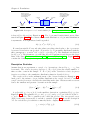
2.4 Probability and Statistics
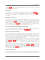
Λ(x| 0, 1)
Λ(x| 0.7, 0.52)
Λ(x| 2, 0, 1)
Density
Density
N(x| 1, 1)
N(x| −1, 0.92)
N(x| 1, 0.82)
−4
−3
−2
−1
0
x
1
2
3
4
0
1
2
3
4
5
6
7
8
9
x
(a) Normal distributions.
(b) Log-normal distributions.
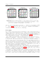
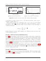
Figure 2.10: Graphs of probability density functions for parameterized normal and lognormal distributions.
Parametric Distribution Families
A number of named probability distributions exists which can be parameterized by one
or more values, e.g. in order to influence its shape or scale. In the following two sections,
the normal and log-normal distributions are described since they are used within this
thesis. Other distribution families include the uniform, the exponential, the gamma, and
the Weibull distributions.
Normal Distribution
The most widely used model for the probability distribution of a random variable is the
normal distribution. It approximates the distribution of a continuous random variable
X which can be modeled by the sum of many small independent variables. It is parameterized by mean µ and variance σ 2 . Its distribution function is denoted by N (µ, σ 2 ) (see
Equation 2.7). The symmetric bell-shaped probability density function is illustrated in
Figure 2.10(a) using three different pairs of parameter values. N (0, 1) is the standard
normal distribution.
N (x | µ, σ 2 ) = P (X ≤ x)
(2.7)
Log-normal Distribution
A positive random variable X is said to be log-normally distributed with two parameters µ and σ 2 if Y = ln X is normally distributed with mean µ and variance σ 2 . A
variable might be modeled as log-normal if it can be thought of as the multiplicative
product of many small independent factors. The 2-parameter log-normal distribution
15
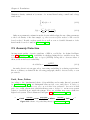
Chapter 2 Foundations
Whisker extends to
smallest data point within
1.5 interquartile ranges
from first quartile
1. quartile
Median
3. quartile
Whisker extends to
largest data point within
1.5 interquartile ranges
from third quartile
Normal
outliers
1.5 IQR
Normal
outliers
1.5 IQR
IQR
1.5 IQR
Extreme
outlier
1.5 IQR
Figure 2.11: Description of a box-and-whisker plot (Montgomery and Runger, 2006).
is denoted by Λ(µ, σ 2 ) (see Equation 2.8). Two log-normal density functions are illustrated in Figure 2.10(b). In contrast to a normal distribution, a log-normal distribution
is asymmetric. It is right-skewed and long-tailed.
Λ(x | µ, σ 2 ) = P (X ≤ x)
(2.8)
If a random variable X can only take values exceeding a fixed value τ , the 3-parameter
log-normal distribution can be used. X is said to be log-normally distributed with the
three parameters τ , µ and σ 2 if Y = ln(X − τ ) is N (µ, σ 2 ). The distribution is denoted
by Λ(τ, µ, σ 2 ). The parameter τ is called the threshold parameter and denotes the lower
limit of the data (Aitchison and Brown, 1957; Crow and Shimizu, 1988). Figure 2.10(b)
contains the density graph of a 3-parameter log-normal distribution.
Descriptive Statistics
Assume that in an experiment, a sample of n observations, denoted by x1 , . . . , xn , has
been made. The relative frequency function f : R 7→ [0, 1] gives the relative number of
times a value occurs in the sample. F : R 7→ [0, 1] is the cumulative relative frequency
function according to the cumulative distribution function described above.
The sample mean x̄ is the arithmetic mean of the observed values (see Equation 2.9).
Analogous to the variance of a probability distribution, the sample variance s2 and the
sample standard deviation s describe the variability in the data. Minimum and maximum
denote the smallest and greatest observations in the sample.
(1) x̄ =
1
n
n
P
i=1
xi ; (2) s2 =
1
n−1
n
P
(xi − µ)2
(2.9)
i=1
A p-Quantile xp , for p ∈ ]0, 1[, is the smallest observation x satisfying F (x) ≥ p (see
Equation 2.10). The quantiles for p = 0.25, p = 0.5, and p = 0.75 are denoted as the 1.,
2. and 3. quartiles. The 2. quartile is also called the median. The interquartile range
(IQR) is the range between the 1. and the 3. quartile. Figure 2.11 shows the description
of a box-and-whisker plot which is commonly used to display these statistics.
xp = min{x | F (x) ≥ p}
16
(2.10)
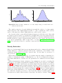
2.4 Probability and Statistics
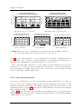
0.035
0.015
0.030
0.025
Density
Density
0.010
0.020
0.015
0.005
0.010
0.005
0.000
0.000
20
40
60
(a) Window size 2.
80
−50
0
50
100
(b) Window size 20.
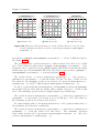
Figure 2.12: Kernel density estimations of a data sample using a normal kernel and
different window sizes.
The outside points in a box-and whisker plots mark the outliers of a data sample.
Value between 1.5 and 3 IQRs farther from the 1. or the 3. quartile are called (normal)
outliers. All values more than 3 IQRs farther are called extreme outliers.
An observation that occurs with the highest frequency is called the mode. Data with
more than one mode is said to be multimodal. A sample with one mode is called unimodal.
A sample with two modes is called bimodal. Generally, for symmetric distributions mean,
median, and mode coincide. If mean, median, and mode do not coincide, the data is said
to be skewed (asymmetric, with a longer tail to one side) (Montgomery and Runger,
2006). It is right-skewed if mode < median < mean and left-skewed if mode > median >
mean.
Density Estimation
Often one obtains sample data from an experiment and needs to estimate the underlying
density function fˆ. Density estimation denotes the construction of an estimate of the
continuous density function from the observed data. It can either be parametric or
non-parametric (Silverman, 1986).
When using the parametric strategy, one assumes that the sample is distributed according to a parametric family of distributions, e.g. the above-mentioned normal or
log-normal distributions. In this case, the parameters are estimated from the sample
data.
With non-parametric density estimation, less assumptions are made concerning the
distribution. A popular non-parametric estimation is the kernel estimator as in Equation 2.12. Based on the observations xi from the sample data, the density at a point x is
estimated by summing up the weighted distance between x and all observations xi within
a given window width h around each observation. The distances are weighted by a kernel
function K which satisfies the condition in Equation 2.11. If K is a density function
such as the normal distribution, fˆ is a density function as well. The window width h is
also called the smoothing parameter or the bandwidth. When h is small, spikes at the
observations are visible whereas with h being large, all detail is obscured. Figure 2.12
17
Chapter 2 Foundations
illustrates density estimation by means of a normal kernel using a small and a large
window size.
Z∞
K(x)dx = 1
(2.11)
−∞
n
1X1
fˆ(x) =
K
n i=1 h
x − xi
h
(2.12)
Other non-parametric estimation methods exist which adapt the smoothing parameter
to the local density of the data sample, e.g. the nearest neighbor method or the variable
kernel method. Details on these methods as well as a more detailed discussion of the
kernel method can be found in (Silverman, 1986).
2.5 Anomaly Detection
An important quality of service attribute of EIS is availability. As defined in Equation 2.13 (Musa et al., 1987), availability is calculated using the two variables mean time
to failure (MTTF) and mean time to repair (MTTR). Being able to decrease either of
them yields an increased availability.
Availability =
MTTF
MTTF + MTTR
(2.13)
Anomaly detection is an approach to increasing availability by reducing repair times.
Errors or failures, as defined in the following paragraph, shall be detected early or even
proactively.
Fault, Error, Failure
According to the “fundamental chain of dependability and security threats” presented
by Avižienis et al. (2004), we distinguish between fault, error, and failure. A fault, e.g.
a software bug, implies an error as soon as it has been activated. An error is that
part of a corrupt system state which itself may cause a failure, i.e. an incorrect system
behavior observable from outside the system. Moreover, a failure may cause a fault in a
higher-level system. This is illustrated in Figure 2.13 (Avižienis et al., 2004).
...
fault
activation
error
propagation
failure
causation
fault
Figure 2.13: Chain of dependability threats (Avižienis et al., 2004).
18
...
2.5 Anomaly Detection
Approach
A common approach for detecting anomalies is building a model of a system’s “normal
behavior” in terms of a set of monitored parameters, and comparing this model with
a dynamically generated model of the respective current behavior in order to uncover
deviations (Kiciman, 2005). The data being monitored can be obtained from different
levels, e.g. network, hardware or application level. Typically the model of the normal
behavior is created based on data monitored in a learning phase. Current system behavior
is monitored and compared with the learned model in the monitoring phase which is the
system in its productional use. If an adaptive approach is used, the normal behavior is
updated with new data in the monitoring phase.
Thus, anomaly detection contributes to failure detection in that way, that anomalies
are assumed to be indicative for failures. As soon as failures are detected, techniques
can be used to localize the root cause. In the following section we present a selection
of existing approaches covering anomaly detection in software systems. An approach by
Agarwal et al. (2004) is presented in Section 2.9.
Examples
Chen et al. (2002) present an approach for detecting anomalies in component-based
software systems and isolating their root cause. By having instrumented the middleware
underlying the application to be monitored, the set of components used to satisfy a user
request is captured. Internal and external failures, such as failing assertions or failing
user requests, are detected. In a data clustering analysis, sets of components which are
highly correlated with failures are discovered in order to determine the root cause.
Kiciman and Fox (2005) present an approach for detecting anomalies of internal system
behavior in terms of component interaction. Based on the framework mentioned in the
previous paragraph (Chen et al., 2002), they capture component interactions and path
shapes. Two components (or component classes) interact with each other if one uses
the other to service a request. A path shape is defined as “an ordered set of logical
components used to service a client request”. The approach is divided into three phases:
observation, learning and detection phases. While observing and learning, the path
shapes and component interactions are derived from monitored data. A reference model
of the application’s normal behavior in terms of the above-mentioned characteristics is
build. Sets of path shapes are modeled by a probabilistic context-free grammar (PCFG).
In the detection phase, anomalies in the current behavior are searched with respect to
the reference model, using anomaly scores to determine whether an observed shape is
anomalous.
Based on the correlations between input and internal system behavior variables, Chen
et al. (2006) present an approach for anomaly detection. Both sets of variables are transformed into a number of correlating pairs. Based on a threshold, the system variables are
divided into those having a highly correlated input partner and those being uncorrelated
or having a low correlated partner. The correlation for the highly correlated system
variables and its input is recalculated during operation in order to detect deviations as
indicators of failing behavior. The low correlated variables are monitored with respect to
19
Chapter 2 Foundations
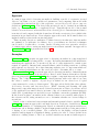
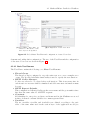
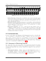
Figure 2.14: JMeter GUI. The hierarchical Test Plan is shown in the left-hand side of the
window. The right-hand side contains an HTTP Request Sampler configuration
dialog.
a statistic capturing the activity of variables. Again, a threshold is used as an anomaly
indicator.
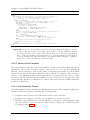
2.6 Apache JMeter
Apache JMeter (Apache Software Foundation, 2007b) is a Java-implemented workload
generator mainly used for testing Web applications in terms of functionality and performance. This section contains a description of those aspects relevant for our work.
Overview
Traces are defined by a Test Plan which is a hierarchical and ordered tree of Test Elements. The number of users to be emulated, as well as other global parameters such as
the duration of the test, i.e. the trace generation phase, are configured within a Thread
Group element forming the root of a Test Plan. The core Test Elements are Logic Controllers and Samplers. Logic controllers group Test Elements and define the control
flow of a Test Plan. Samplers are located at the leaves of the tree and send the actual
requests. Examples for Logic Controllers are If and While Controllers which have an
intuitive meaning known from programming languages. HTTP Request or FTP Request
are examples for Samplers and are located at the leaves of the Test Plan.
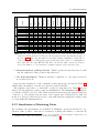
JMeter provides a graphical user interface (GUI) for creating a Test Plan and executing
the test. Figure 2.14 shows the JMeter GUI. Existing Test Plans can also be executed
in non-GUI mode in order to save system resources.
20
2.6 Apache JMeter
Apache JMeter
start and stop
GUI
Non−GUI
Engine
reads configu−
ration from
initializes
and controls
Test Plan
modifies
and creates
Thread Group
(configuration)
contains
number of
Thread
executes
instance of
Test Plan
(instance)
JMeter Test Elements
GUI Classes
Test Element Classes
control.gui
control
samplers
samplers.gui
config.gui
config
assertions.gui
assertions
...
...
stored as
JMX
Figure 2.15: JMeter Architecture.
Additional Test Elements include Timers, Listeners, Assertions, and Configuration
Elements. Timers add a think time, e.g. constant or based on a normal distribution,
between Sample executions of the same thread. Assertions are used to make sure that
the server responds the expected results, e.g. it contains a certain text pattern. By using
Listeners, results of the Sample executions can be logged, e.g. HTTP response codes or
failed assertions. The set of Configuration Elements includes an HTTP Cookie Manager
to enable client-side cookies as well as Variables. Table A.1 lists all Test Element types
included in JMeter version 2.2. The user’s manual (Apache Software Foundation, 2006)
contains a description of functionality and available parameters of all Test Elements.
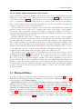
Architecture
JMeter includes components required for the GUI and non-GUI mode, for holding the
configuration of the Test Plan, and those required for the test execution. This categorization is illustrated by the pillars shown in Figure 2.15.
GUI components provide the functionality to graphically define a Test Plan and to
start and stop the test execution. As mentioned above, test can also be started in nonGUI mode. The Engine is responsible for controlling the test run. It initializes the
Thread Group and the included Threads each of which is assigned a private instance of
the Test Plan to be executed.
21
Chapter 2 Foundations
Client
HTTP
HTTP
struts.ActionServlet
iBatis JPetStore
Apache Struts
Presentation Layer
Service Layer
Persistence Layer
iBatis DAO Framework
SQL
SQL
DBMS
(a)
(b)
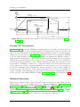
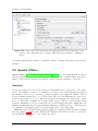
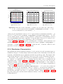
Figure 2.16: JPetStore index page.
A Test Plan is internally represented by a tree of Test Element classes itself representing
the respective element in Test Plan. A Test Plan can be saved in a file with an XMLbased JMX format. In addition to the configuration parameters, the Test Element classes
contain the implementation of the Test Element’s behavior.
Any Test Element class has an associated GUI class providing a configuration dialog for
the Test Element. It is responsible for creating and modifying the related Test Element
classes. Figure 2.14 shows the dialog for configuring an HTTP Request Sampler.
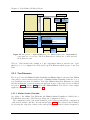
2.7 JPetStore Sample Application
JPetStore is a sample Java Web application that represents an online shopping store
offering pets. In the following two sections, those details which are relevant for our work
are described.
Overview
The application has originally been developed to demonstrate the capabilities of the
Apache iBATIS persistance framework (Apache Software Foundation, 2007a). It is based
on the J2EE sample application Java Pet Store (Sun Microsystems, Inc., 2006) which has
been used in a variety of scientific studies, e.g. (Chen et al., 2005; Kiciman and Fox,
2005).
22
2.8 Tpmon
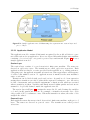
An HTML Web interface provides access to the application (see Figure 2.16(a)). The
catalog is hierarchically structured into categories, e.g. “Dogs” and “Cats”. Categories
contain products such as a “Bulldog” and a “Dalmation”. Products contain the actual
items, e.g. “Male Adult Bulldog” and “Spotted Adult Female Dalmation”, which can be
added to the virtual shopping cart, the content of which can later be ordered after having
signed on to the application and having provided the required personal data, such as the
shipping address and the credit card number.
Architecture
The architecture is made up by three layers, i.e. the presentation layer, the service layer
and the persistence layer. Clients communicate with the application through the HTML
Web interface using the HTTP request/response model (see Section 2.1). A database
holds the application data. The architecture is illustrated in Figure 2.16(b).
The presentation layer is responsible for providing the user interface which gives a
view of the internal data model and its provided services. The layer is realized using
the Apache Struts framework (Apache Software Foundation, 2007a) which includes the
so-called ActionServlet constituting the application entry point (see Section 2.1).
The service layer maintains the internal data model and actually performs the requested services. Data is accessed and modified through the persistence layer.
For each component of the data model, data access objects (DAOs) exist within the persistence layer acting as an interface to the database. The DAOs and the actual database
access are realized using the Apache iBATIS persistance framework which provides a
common interface to SQL-based relational database management systems. Table 4.5
gives an overview of the tables contained in the database schema of the application.
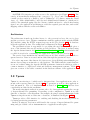
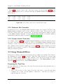
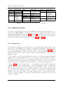
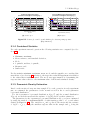
2.8 Tpmon
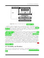
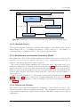
Tpmon is a monitoring tool which can be integrated into Java applications in order to
monitor the response times (see Section 2.2) of operations as well as other applicationlevel information. The core implementation is based on Focke (2006) but has been
considerably modified in the meantime.
The monitoring functionality is woven into the code of an application using the concept
of Aspect-Oriented Programming. Depending on the configuration, Tpmon stores the
data into a database or the filesystem. An example, showing a system instrumented with
Tpmon storing the monitored data into a database, is illustrated in Figure 2.17(a).
Tpmon provides a Web interface for enabling and disabling the monitoring as well as
for setting monitoring parameters.
In the following two sections we will describe the concept of Aspect-Oriented Programming and give details on how instrumentation of applications takes place.
23
Chapter 2 Foundations
SQD Call of Annotated Operation
CPD Tpmon Integration
a
<<execution environment>>
b
a()
b()
M
M
a
M
b
M
c
point−cut
match
@TpmonMonitoringProbe()
public void b(){
...
}
AOP
TPMon
pointcut probeMethod():
execution(@TpmonMonitoringProbe * *.*(..));
aspect
Object around(): probeMethod() {
start=getTime();
proceed(); //actually execute b.b()
stop=getTime();
insertMonitoringData(getOperationName,start,stop);
}
SQL
SQL
DBMS
(a) In an execution environment, three components a,
b and c each provide services which are monitored
by means of Tpmon using the AOP concept. Tpmon stores the monitored data into the database.
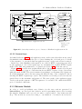
(b) Component a calls operation b
of component b. This operation contains a point-cut defined
by the annotation @TpmonMonitoringProbe. As defined in the
description of the respective aspect probeMethod, Tpmon saves
the current time before and after
b is executed.
Figure 2.17: Sample system instrumented with Tpmon (a) and how an annotated operation is woven (b).
aspect
weaver
basic functionality program
aspect
programming
languages
woven output code
aspect
description
programs
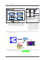
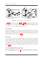
Figure 2.18: An aspect weaver weaves the aspects and the functional part of an application into a single binary (following (Kiczales et al., 1997)).
24
2.8 Tpmon
Aspect-Oriented Programming
Often, application code is tangled with cross-cutting concerns which are not directly
responsible for application functionality. Examples are logging, error handling, and performance measurement. In a certain way it may be possible to capsulate those concerns
by procedure abstraction, but often this still leads to code which is hard to maintain.
Aspect-Oriented Programming (AOP) is a concept which strives to separate crosscutting concerns from application functionality as far as possible (Kiczales et al., 1997).
The cross-cutting concerns are called aspects and are expressed in a form which is separate
from the application code. Positions in the code to which aspects are to be woven are
called point-cuts. A so-called aspect weaver automatically combines the application and
the aspects into binaries. Following Kiczales et al. (1997), the procedure of enriching an
application with aspects using AOP is illustrated in Figure 2.18.
AspectJ (Eclipse Foundation, 2007) is an AOP extension to the Java programming
language. The AspectJ weaver allows for weaving aspects into an application at compiletime, post-compile time, and load-time (AspectJ Team, 2005). Independent of the time
the weaving takes place, the AspectJ weaver produces equal Java binaries. Using compiletime weaving, the AspectJ compiler weaves the aspects to the defined point-cuts inside
the application sources. When using post-compile time weaving, the aspects are woven
into the already existing application binaries. Thus, post-compile time weaving is also
denoted as binary weaving. In order to use load-time weaving, an AspectJ weaving agent
is registered inside the Java virtual machine tool interface (JVMTI ) (Sun Microsystems,
Inc., 2004) and basically performs binary weaving at the time a class to be woven is loaded
by the class loader. Point-cuts inside the application can be defined within external
configuration files without modifying the application’s source code or by enriching the
application code with annotations which were introduced with Java 5.
Instrumentation Modes
Tpmon is based on the AOP extension AspectJ. A configuration file contains a specification of classes to be considered by the weaving agent, e.g. by using the directive
<include within=”com.ibatis.jpetstore ..∗ ”/>, any of the JPetStore classes (see Section 2.7) the
name of which matches the given pattern would be considered. In order to consider the
application entry operations of the presentation layer as well, one would also include the
pattern org.apache.struts.ActionServlet. The preferred weaving method is load-time
weaving – one of the weaving alternatives mentioned above.
Tpmon offers the two below-described instrumentation modes, i.e. the way operations
to be monitored are specified.
1. Full Instrumentation Mode: Using this mode, the weaving agent weaves the
monitoring functionality into all operations in those classes specified in the configuration file. No source code modifications are necessary.
2. Annotation Mode: Using this mode, all methods to be monitored need to be
labeled by the Java annotation @TpmonMonitoringProbe. Additionally, the related
class must be specified in the configuration file.
25
Chapter 2 Foundations
As soon as the execution of an instrumented operation starts, Tpmon stores the current timestamp. The same holds when the method returns. Start time tin and stop
time tout as well as the below-listed data form the monitoring entry for this invocation.
Figure 2.17(b) illustrates how the weaving takes place for an annotated method.
• experimentid: A unique identifier for the current experiment.
• operation: The full operation name consisting of class and method name, e.g.
com.ibatis.jpetstore.presentation.CatalogBean.viewCategory().
• sessionid, traceid: The application-level session and trace identifier as described
in Sections 2.1 and 2.3.
2.9 Related Work
Work directly related to ours covers the characterization and generation of workload for
Web-based systems, the analysis of response time in enterprise applications as well as
timing behavior anomaly detection.
The results of workload characterization for specific enterprise application in real use
are presented in a number of papers. For example, Arlitt et al. (2001), Menascé et al.
(2000), and Menascé and Akula (2003) analyzed online bookstores, shopping systems,
and auction sites. Menascé et al. (2000) suggest a hierarchical workload model for Webbased systems consisting of a session layer, a functional layer, and an HTTP request
layer (see Section 2.3).
Many freely available and commercial Web workload generators exist, e.g. Mercury
LoadRunner (Mercury Interactive Corporation, 2007), OpenSTA (OpenSTA, 2005), Siege
(Fulmer, 2006), and Apache JMeter (Apache Software Foundation, 2007b) (see Section 2.6).
In many performance-related experiments, simple techniques were used to generate
synthetic workload. For example, Cohen et al. (2005) used the standard request generator
httperf (Mosberger and Jin, 1998) to generate workload for the Java Pet Store. In this
case, the order of issued requests within a session was dynamically determined using
probabilities.
Menascé et al. (1999) defined a Customer Behavior Model Graph (CBMG) to formally model the user behavior in Web-based systems using Markov chains. Shams et al.
(2006) state that CBMGs are inappropriate for modeling valid users sessions and present
Extended Finite State Machines (EFSM) which include additional elements such as predicates and actions. Ballocca et al. (2002) propose an integration of CBMGs and a Web
stressing tool to generate realistic workload. In Section 2.3 we provided a detailed description of these approaches.
Mielke (2006) statistically analyzed the end-to-end response times of transactions in
three Enterprise Resource Planning (ERP) systems in real use. The response times
were measured with built-in performance measurement tools. The main contributions
to the response times were caused by process time and database request time. Mielke
found out that the distributions of the data samples could be estimated by the log-normal
distribution – including body and tail. Sample mean and variance from the response time
26
2.9 Related Work
data were used as the parameters for the probability density function of the log-normal
function. Deviations from the log-normal distributions occurred and were often caused
by performance problems. Thus, Mielke suggests to use response time distributions to
locate performance problems in ERP systems.
Agarwal et al. (2004) combined dependency graphs and monitored response time samples from system components for problem determination, i.e. detecting misbehavior in a
system and locating the root cause. Agarwal et al. assume existing end-user service level
agreements (SLAs) with specified end-to-end response time thresholds for each transaction type. Dependency graphs model the relation between components in terms of
synchronous or asynchronous invocations among each other. At run-time, a so-called dynamic threshold is computed for each component based on average component response
times. As soon as a SLA violation is detected, all components are classified into good
and bad behavior depending on whether or not they are affected by the problem, i.e.
they exceed their dynamic threshold or are in a relation with components exceeding
their dynamic threshold. The components in a bad state are ranked in order of their
current response time samples compared with the dynamic threshold in order to determine the root cause of the problem. Agarwal et al. claim that by using their dynamic
threshold approach, changes in operating conditions, such as workload changes, can be
accommodated.
27
Chapter 3
Probabilistic Workload Driver
This chapter deals with the development of the workload driver used in the case study.
We introduce an approach for a model-based definition and generation of probabilistic
workload for enterprise applications. The definition of the user behavior is separated
from application- and protocol-specific details. The models are based on hierarchical
finite state machines and Markov chains. We implemented our approach by extending the existing workload generator JMeter (see Section 2.6). This extension named
Markov4JMeter has been released under an open source license (van Hoorn, 2007).
Section 3.1 contains the requirements definition of the workload driver. The conceptual design of the workload driver including the definition of the workload configuration
and execution semantics are given in Section 3.2. Section 3.3 outlines the resulting implementation and integration into JMeter. A description on how to model and generate
probabilistic workload with Markov4JMeter is illustrated in Section 3.4.
3.1 Requirements Definition
The Sections 3.1.1 and 3.1.2 introduce how requirements are labeled and classified in
this requirement definition and states the assumptions made. Which applications and
use cases must be supported is defined in Sections 3.1.3 and 3.1.4. Requirements for the
workload configuration and the provided user interface follow in Sections 3.1.5 and 3.1.6.
3.1.1 Requirements Labeling and Classification
Each requirement is labeled with a unique identifier such as scope::applications(m). An
identifier consists of a descriptive component, in this case scope::applications, and a classification component, which is either m (mandatory) or s (secondary). The classification
is as follows:
Mandatory: A mandatory requirement, emphasized by must, is a requirement which
must be fullfilled in every case.
Secondary: A secondary requirement, emphasized by should , is a requirement which
should be fullfilled. The non-fullfillment of a secondary requirement must be carefully weighted and reasoned.
29
Chapter 3 Probabilistic Workload Driver
UCD Define and Execute Workload
Workload Driver
Define Application and User Behavior Configuration
Define Behavior Mix and Workload Intensity Configuration
Tester
Execute Configured Workload
AUT
Figure 3.1: The use case diagram illustrates the use cases to be supported by the workload driver.
3.1.2 Assumptions
The application which workload is to be generated for is denoted as the application under
test (AUT). The term tester relates to the person using the workload driver.
The workload configuration is divided into an application and user behavior configuration and a behavior mix and workload intensity configuration.
• The application and user behavior configuration contains the application- and
protocol-specific details required to generate valid workload. Moreover, it includes
models of the probabilistic user behavior for the AUT.
• The behavior mix and workload intensity configuration contains the information
related to a specific workload execution, e.g. the used application and user behavior
configuration, the relative distribution of behavior models to use as well as the
number of simulated users and the duration of the execution.
3.1.3 Supported Applications
scope::applications(m) - Supported Applications
The workload driver must support applications that satisfy the following properties:
• The application has an HTML Web interface based on the HTTP request/response
model (see Section 2.1) solely using the HTTP methods GET and POST.
• If the application uses sessions, the session identifier is managed by cookies contained
in the HTTP header, by URL-rewriting or by hidden HTML input fields.
• The application does not rely on code embedded in its HTML response that must
be interpreted on client-side, such as JavaScript or AJAX.
30
3.1 Requirements Definition
3.1.4 Use Cases
In this section we define the use cases, the workload driver must support. Each use case
is defined by means of a template containing the fields actors, pre- and post-condition,
as well as a description. Figure 3.1 shows the UML use case diagram.
uc::aum::define(m) - Configure Application and User Behavior
Actors:
Pre-condition:
Post-condition:
Description:
Tester
A new application and user behavior configuration for the AUT
has been created and is accessible to the workload driver.
The user defines and stores an application and user behavior configuration for the AUT (the required configuration parameters
are defined in Section 3.1.5.1).
uc::workloadmix::define(m) - Configure Behavior Mix and Workload Intensity
Actors:
Pre-condition:
Post-condition:
Description:
Tester
The application and user behavior configuration to be used is
accessible.
A behavior mix and workload intensity configuration which can
be executed by the workload driver has been defined.
The user defines and stores the behavior mix and workload intensity configuration (the required configuration parameters are
defined in Section 3.1.5.2).
uc::workload::execute(m) - Execute Configured Workload
Actors:
Pre-condition:
Post-condition:
Description:
Tester, AUT
The workload to be executed has been configured and is accessible to the workload driver (see use cases uc::aum::define(m)
and uc::workloadmix::define(m)).
The workload configuration has been executed by the workload
driver.
The user invokes the workload driver to generate the configured
workload (see Section 3.1.5) for the AUT .
31
Chapter 3 Probabilistic Workload Driver
3.1.5 Workload Configuration
This section contains the requirements for the workload driver configuration. As mentioned above, this configuration is divided into an application-specific application and
user behavior configuration and a behavior mix and intensity configuration for specific
experiment runs.
config:loadstore(m) - Load and Store Configuration
The workload driver must provide functionality to load and store configurations such
that they can be reused. This includes the definition of an appropriate file format.
3.1.5.1 Application and User Behavior Configuration
config::aub::ifaceDetails(m) - Application Interface Definition
A description format must be defined to specify the details on the HTTP communication between client and application under test for all provided interactions.
config::aub::dynValueAssignment(s) - Dynamic Value Assignment
Means should be provided to dynamically assign values for HTTP request parameters. This includes selecting values which depend on the last response, as well as
functionality to select values from prepaired data, e.g. login credentials for user authentication.
config::aub::naviBehaviorModel(m) - User Behavior Model
A description format must be defined to model user session in terms of the issued requests within a session. This must include probabilistic elements to model weighted
alternatives. Varying the assigned probabilities allows for modeling behavior of different behavior classes.
config::aub::userThinkTimesConst(m) - Client-side Think Times (constant)
A constant value to be used as the client-side think times between two subsequent
requests of the same user must be configurable.
config::aub::userThinkTimesDistr(s) - Client-side Think Times (distribution)
Think time distributions should be configurable for each user class to enable think
times that vary based on a parameterizable probability distribution family, such as
the normal distribution. This requirement extends config::aub::userThinkTimes←Const(m).
32
3.2 Design
3.1.5.2 Behavior Mix and Workload Intensity Configuration
config::bmwi::userCountSingle(m) - Single User Count
The workload driver must provide an option to configure the number of concurrent
users to simulate.
config::bmwi::userCountVarying(s) - User Count Variation
The workload driver should provide means to define a varying number of concurrent
users to be simulated, e.g. specified by mathematic formulae depending on the elapsed
experiment time. This requirement extends config::wmic::userCountSingle(m).
config:bmwi:duration(m) - Duration of Workload Execution
The workload driver must provide an option to configure the duration of the workload
execution, e.g. by specifying a time value or by specifying the number of iterations per
user.
config::bmwi::userClassSingle(m) - User Class Assignment
The workload driver must allow to assign a single user class to be used for an entire
workload execution.
config::bmwi::userClassMix(s) - User Class Mix
The workload driver should allow to use multiple user classes during a single workload
execution. The number of users being associated to every single class should then
be relative to the total number of emulated users. This requirement extends con←fig::bmwi::userClassSingle(m).
3.1.6 User Interface
ui::workload::execute(m) - Workload Execution User Interface
The workload driver must provide a command line option to allow batch execution
of previously configured workload (see use case uc::workload::execute).
3.2 Design
This section contains the high-level design of the workload driver which is based on the
requirements definition presented in Section 3.1. In Section 3.2.1 we refine the system
model of the applications to be supported and define basic terms. The workload configuration data model and the design of the architecture and the execution model follow
in Sections 3.2.2 and 3.2.3.
33
Chapter 3 Probabilistic Workload Driver
Data Model of Workload Configuration
CD
0..*
Workload Configuration
− name
0..*
1
1
1
1..*
0..*
User Behavior Model
− thinkTime
− entryState
− finalState
Application Model
User Behavior Mix
1
1
1..*
1
1..*
Protocol State
− uri
− parameters
0..*
1
Protocol Transition
− guard
− action
0..*
1
Application State
1
1
1
Behavioral State
1
0..*
Behavior Assignment
− relativeFrequency
Workload Intensity
0..*
− duration
− sessionArrivalFormula
1
0..*
Application Transition
− guard
− action
1
1
Behavioral Transition
− probability
Figure 3.2: Class diagram of the workload configuration data model including the basic
elements application model, a set of user behavior models related to the application
model, as well as a definition of the user behavior mix and the workload intensity.
3.2.1 System Model
We consider a system model which is based on the system model presented in Section 2.1
and on the hierarchical workload model presented in Section 2.3.
An EIS provides a number of services. An invocation of a service involves the invocation
of possibly more than one request on protocol level. A series of consecutive and related
requests to the system issued by the same user is called a session. As soon as the first
request has been issued, the user begins a new session which is then denoted as an active
session until the last request has been issued. The time interval elapsed between the
completion of a server response and the invocation of the next one is denoted as the
think time.
3.2.2 Workload Configuration Data Model
Based on the requirements related to the workload configuration (see Section 3.1.5) including the application and user behavior configuration and the behavior mix and intensity configuration, we defined a workload configuration data model. It consists of an
application model, a set of user behavior models related to the application model as well
as a definition of the user behavior mix and the workload intensity. The configuration
elements are described in the following Sections 3.2.2.1–3.2.2.4. Figure 3.2 shows the
class diagram for this data model.
34
3.2 Design
Figure 3.3: Sample application model illustrating the separation into session layer and
protocol layer.
3.2.2.1 Application Model
The application model contains all information required by the workload driver to generate valid sessions for an application. It is a two-layered hierarchical finite state machine
consisting of a session layer on top and a protocol layer underneath. Figure 3.3 shows a
sample application model.
Session Layer
The session layer consists of a non-deterministic finite state machine. The states are
denoted as application states. The transitions are called application transitions. Each
application state is related to a service provided by the application, e.g. adding an item to
a shopping cart. An application transition between two states represents a valid sequence
of service calls within a session. No application state is marked as the state machine’s
entry or exit state.
Transitions can be labeled with guards and actions. A guard is a boolean expression
stating that a transition can only be taken if the expression evaluates to true. An action
is a list of statements, such as variable assignments or function calls, which are executed
when a transition is taken. Variables and functions used within guards and actions are
assumed to be globally defined outside the application model.
The session layer in Figure 3.3 contains the states S0, S1, and S2 using the variables
a, b, and c in the guards and actions. For example, a transition from state S2 to S1 is
only possible if b! = 0 evaluates to true. When this transition is taken, the value of b is
assigned the value 1.
Protocol Layer
Each application state has an associated deterministic finite state machine on the protocol
layer. The states are denoted as protocol states. The transitions are called protocol
transitions.
35
Chapter 3 Probabilistic Workload Driver
0.5
0.1
Exit
Exit
0.4
0.2
0.1
0.7
S1
S1
0.7
0.3
0.5
0.2
S0
Exit
Exit
S0
S2
0.1
0.1
0.3
0.05
0.4
Exit
Exit
0.6
0.1
0.65
(a) User behavior model BA,0 .
S2
(b) User behavior model BA,1 .
Figure 3.4: Transition diagrams of user behavior models BA,0 and BA,1 .
A state machine is executed when the related application state is entered and models
the sequence of protocol-level requests to be invoked (see Section 3.2.1). Analogous to
the session layer, transitions between states may be labeled with guards and actions using
the same global variables and functions.
For example, the state machine related to the application state S0 in Figure 3.3 contains the three protocol states a.shtml, b.shtml, and c.shtml that correspond to HTTP
request URIs. After the request for a.shtml has been issued, the next state depends on
the outcome of the evaluation of the expression a > 0 in the guard.
3.2.2.2 User Behavior Model
A user behavior model consists of a Markov chain (see Section 2.3) and a mathematical
formula modeling the client-side think time. It is associated with an application model
and each state of the Markov chain relates to an application state.
Formally, we define a user behavior model BA for an application A as a tuple (Z ∪
{Exit}, P, z0 , ftt ). Z denotes the set of states contained in the Markov chain with entry
state z0 . The state Exit is the dedicated exit state which has no related application state.
P denotes the transition matrix. ftt contains the think time formula.
Figure 3.4 shows the transition diagrams of two user behavior models BA,0 and BA,1
for the application model shown in Figure 3.3. Both user behavior models solely differ
in their transition probabilities.
3.2.2.3 User Behavior Mix
A user behavior mix BMIXA for an application model A is a set {(BA,0 , p0 ), . . . ,
(BA,n−1 ,pn−1 )} assigning relative frequencies pi to user behavior models BA,i . The property in Equation 3.1 must hold.
n−1
X
pi = 1
(3.1)
i=0
A tuple (BA,i , pi ) states that user sessions based on the user behavior model BA,i occur
with a relative frequency pi ∈ [0, 1] during workload execution.
36
3.2 Design
CD
High−Level Overview of Workload Driver
Engine
1
includes >
1
includes >
1
1
behavior model assigned by >
initializes and controls
>
1
0..*
Behavior Mix Controller
0..*
User Simulation Thread
0..*
1
session entrance
scheduled by >
1
Session Arrival Controller
Figure 3.5: Architecture overview of workload driver in UML class diagram notation.
3.2.2.4 Workload Intensity
The workload intensity configuration includes the definition of the duration and a mathematic function R≥0 7→ N defining the number of active sessions, i.e. the number of
concurrent users, to simulate relative to the elapsed experiment time.
3.2.3 Architecture and Iterative Execution Model
The architecture of the workload driver includes a workload driver engine, a behavior mix
controller, a session arrival controller, and a pool of user simulation threads the size of
which is constant throughout the entire execution.
The workload driver engine initializes and controls the other components based on a
workload configuration as defined in the previous Section 3.2.2. Each user simulation
thread represents one user at a time and issues the requests based on a session model
which is composed by the application model and a user behavior model assigned by the
behavior mix controller. The session arrival controller controls the respective number of
active sessions.
A more detailed description of components is given in the following Sections 3.2.3.1–
3.2.3.3. Figure 3.5 shows a UML class diagram illustrating how they are related.
The composition and execution of the probabilistic session model is described in Section 3.2.3.4.
3.2.3.1 Behavior Mix Controller
The behavior mix controller maintains the assignment of user behavior models to user
sessions executed by the user simulation threads. The assignment is performed based
on the relative frequencies configured in the behavior mix which is part of the workload
configuration.
37
Chapter 3 Probabilistic Workload Driver
Method e x e c u t e S e s s i o n ;
begin
a r r i v a l C t r l . e n t e r S e s s i o n ( ) ; /∗ r e q u e s t s e s s i o n e n t r a n c e ∗/
z ← BA . z0 ; /∗ s e t c u r r e n t s t a t e t o e n t r y s t a t e ∗/
T ← e n t e r ( z ) ; /∗ e n t e r a p p l i c a t i o n s t a t e ∗/
while z 6= BA . E do
/∗ f e t c h t r a n s i t i o n s whose g u a r d s e v a l u a t e t o t r u e ∗/
t r u e L i s t ← hi ; probSum ← 0 . 0 ; cumPropList ← hi ;
f o r each t ∈ T do
i f e v a l u a t e ( t . guard ) then
t r u e L i s t ← t r u e L i s t • hti
cumProbSum ← cumProbSum + BA . P [ z , t.z ] ;
cumProbList ← cumProbList • hti
fi ;
done ;
/∗ s e l e c t t r a n s i t i o n based on t r a n s i t i o n p r o b a b i l i t i e s ∗/
rndVal ← random ( cumProbSum ) ;
z ← trueList [ 0 ] ;
f o r i ∈ 0. . .cumProbList . l e n g t h −2 do
i f rndVal < cumProbList [ i ] then break ;
else z ← t r u e L i s t [ i +1];
done ;
/∗ e x e c u t e a c t i o n and e n t e r a p p l i c a t i o n s t a t e ∗/
evaluate (t . action ) ; T ← enter ( z ) ;
done ;
a r r i v a l C t r l . e x i t S e s s i o n ( ) ; /∗ n o t i f y we q u i t our s e s s i o n ∗
end ;
Figure 3.6: Sketch of core algorithm executed by each user simulation thread to execute
a session. BA denotes the user behavior model (Z, P, z0 , E, ftt ) which has already
been assigned based on the behavior mix. The method enter executes the application
state z passed as parameter and returns the set of outgoing transitions. The method
evaluate evaluates the expression passed as parameter and returns the evaluation
result. The operator • is used to concatenate lists.
3.2.3.2 Session Arrival Controller
The session arrival controller controls the number of active user sessions during workload
generation. It provides a session entrance and exit protocol for the user simulation
threads. Before entering a session, the method enterSession() must be called which
may block the thread in a queue until the session entrance is granted. After leaving a
session, a user simulation thread invokes the method exitSession() in order to notify
the session arrival controller that the number of active session can be decremented. The
session arrival controller is configured according to the active sessions formula within the
workload configuration.
3.2.3.3 User Simulation Threads
Each user simulation thread iteratively emulates users based on the configured application
and user behavior models by executing the following steps:
1. Request a user behavior model from the behavior mix controller.
2. Request session arrival controller for a permission to execute a session.
3. Execute a probabilistic session model which is a composition of the application and
the user behavior model assigned for this iteration. This step is described in the
following Section 3.2.3.4.
38
3.3 Markov4JMeter
3.2.3.4 Session Model Composition and Execution
Sessions executed by the user simulation threads are based on probabilistic session models
which are a composition of the application model (see Section 3.2.2.1) and a user behavior model (see Section 3.2.2.2). As mentioned above, the application model contains the
protocol information and constraints required to generate valid sessions for an application. A user behavior model contains information about the probabilistic navigational
behavior as well as a model of the think times.
The two models are directly related by associated states and transitions contained in
the user behavior model (the set Z of states) and on the session layer of the application model. The composition of the two models to a single probabilistic model can be
performed straightforward by enriching the application transitions with the probabilities
contained in the user behavior model.
Starting with the entry state z0 defined in the user behavior model, a probabilistic
session model is executed as follows. Given a current state, the next state is determined
by first evaluating the guards of the outgoing transitions related to the current state.
One of these transition is randomly selected based on their assigned probabilities. The
action of the selected transition is executed and the requests towards the application are
issued by traversing the determinitic state machine of the state within the protocol layer
of the application model. A session ends when the determined transition leads to the
destination state Exit which is the exit state of the user behavior model.
The semantic of the composition of an application model and a user behavior model
is illustrated in Figure 3.6 using a pseudo-code notation for the code executed by a
user simulation thread in each iteration. We assume that the user behavior model
BA = (Z, P, z0 , E, ftt ) has been assigned already. The tuple elements are accessed by
means of BA .Z, BA .P , BA .z0 and BA .E. First, the user simulation thread invokes a
request to enter the session towards the session arrival controller. The thread may get
blocked at this point, i.e. it might be put into a queue. This is the case when the number
of active sessions would exceed the allowed number of active sessions if this entrance
would be granted.
3.3 Markov4JMeter
A workload driver following the design presented in the previous Section 3.2 has been
implemented and integrated into the existing workload generator JMeter (see Section 2.6)
as an extension called Markov4JMeter.
Markov4JMeter includes the Test Elements Markov Session Controller and Markov State
which allow the definition of a probabilistic session model within a JMeter Test Plan. The
Test Elements are described in Section 3.3.1. The additional components Behavior Mix
Controller and Session Arrival Controller are described in Sections 3.3.3 and 3.3.4. Behavior
models are stored in external files. The file format will be described in Section 3.3.2.
Figure 3.7 illustrates how the Markov4JMeter components are integrated into JMeter.
The conceptual workload driver components workload driver engine and user simulation threads defined in Section 3.2.3 are realized by the JMeter components Engine and
39
Chapter 3 Probabilistic Workload Driver
Non−GUI
Engine
Test Plan
Session
Arrival
Controller
(configuration)
Behavior
Mix
Controller
Thread Group
Thread
Test Plan
(instance)
reads models from
configured by
GUI
JMeter Test Elements
Markov4JMeter Test Elements
markov4jmeter.controller.gui
markov4jmeter.controller
MarkovSessionControllerGui
extends AbstractControllerGui
MarkovSessionController
extends GenericController
SessionArrivalFormulaPanel
BehaviorMixPanel
SessionArrivalFormula
BehaviorMix
MarkovStateGui
extends AbstractControllerGui
MarkovState
extends GenericController
ApplicationTransitionsPanel
ApplicationTransitions
JMX
refers to
Behavior
Files
(CSV)
Figure 3.7: Integration of Markov4JMeter into the JMeter architecture. Markov4JMeter
components are colored blue. The Test Elements are divided into a GUI class and
a Test Element class.
Threads. This includes the definition of the experiment duration and the size of the
thread pool to be configured in a Thread Group Test Element which is part of any Test
Plan.
3.3.1 Test Elements
The Logic Controllers Markov Session Controller and Markov State both extend the JMeter
class jmeter.control.GenericController. A Markov Session Controller forms the root of
a probabilistic session model within a Test Plan. Markov State Test Elements are added
directly underneath, each representing an application state of the session layer as defined
in Section 3.2.2.1. Figure 3.8(a) shows the Markov4JMeter Test Plan for the sample
application model illustrated in Figure 3.3.
3.3.1.1 Markov Session Controller
According to the JMeter Test Elements, the Markov Session Controller is divided into a
Test Element class and a GUI class providing the configuration dialog.
The configuration dialog allows the definition of the behavior mix and the configuration
of the session arrival controller. It is shown in Figure 3.8(b). The behavior mix is defined
by selecting the respective behavior files and specifying the desired relative frequencies.
40
3.3 Markov4JMeter
(a) Test Plan.
(b) Markov Session Controller configuration dialog.
(c) Markov State configuration dialog.
Figure 3.8: Probabilistic Test Plan and Markov4JMeter configuration dialogs.
The formula defining the number of allowed active sessions during the test execution
must evaluate to a positive integer.
The Test Element class contains the implementation of the session model composition and execution as described in Section 3.2.3.4. In each iteration, i.e. each time a
new session is to be simulated, the Markov Session Controller requests a behavior from
the Behavior Mix Controller and requests the Session Arrival Controller to start the execution of this session. An iteration ends when the exit state of the behavior model (see
Section 3.3.2) is reached.
3.3.1.2 Markov State
As the implementation of the Markov Session Controller, the Markov State is divided into
a Test Element class and a GUI class.
Any subtree of JMeter Test Elements can be added to an Markov State representing
the related deterministic state machine on the protocol layer of the application model.
The configuration dialog of the Test Element allows the definition of the state transitions with guards and actions using JMeter’s variables and functions. The list of transitions is refreshed as the list of Markov States underneath the related Markov Session
Controller is modified.
For example, the Markov State S0 in Figure 3.8(c) contains the HTTP Samplers f.shtml
and g.shtml which are executed in this order according to the application model in
Figure 3.3. The configuration of the transitions is shown in Figure 3.8(c).
3.3.2 Behavior Files
The transition matrix of a user behavior model as defined in Section 3.2.2.2 is stored in
external files using a comma-separated value (CSV) file format. It contains the names of
all Markov States underneath a Markov Session Controller. The entry state of the model
is marked with an asterisk (at most one). The column labeled with $ represents the
transition probability towards the exit state.
41
Chapter 3 Probabilistic Workload Driver
Figure 3.9 shows the behavior file of the user behavior model in Figure 3.4(a). Valid
behavior file templates can be generated through the Markov Session Controller configuration dialog.
, ”S0 ”
”S0 ∗ ” , 0 . 0 0
”S1 ” , 0 . 0 0
”S2 ” , 0 . 1 0
,
,
,
,
”S1 ”
0.70
0.50
0.50
,
,
,
,
”S2 ”
0.10
0.10
0.00
,
,
,
,
”$ ”
0.20
0.40
0.40
Figure 3.9: User behavior model stored in CSV file format.
3.3.3 Behavior Mix Controller
As mentioned above, the Behavior Mix Controller assigns user behavior models to the
Markov Session Controller based on the configured behavior mix. The models are read
from the behavior files and converted into an internal representation which is passed
to the Markov Session Controller. A single Behavior Mix Controller is available which is
implemented using the singleton pattern (Gamma et al., 2000).
3.3.4 Session Arrival Controller
According to Section 3.2.3.2, the Session Arrival Controller provides the methods enterSession() and exitSession() which are called by the Markov Session Controller before
starting to execute a new session. Depending on the current number of active sessions and
the configured active sessions formula (see Section 3.2.2.4), a thread might get blocked
until the session entrance is granted. The Session Arrival Controller is also implemented
using the singleton pattern.
3.4 Using Markov4JMeter
This section contains a step-by-step description how a simple probabilistic Test Plan for
the JPetStore (see Section 2.6) is created. This Test Plan can then be executed just
like any ordinary JMeter Test Plan. The JMX file of the Test Plan and the associated
files can be found in the directory examples/jpetstore/ of the Markov4JMeter release.
Appendix A.2 describes how to install Markov4JMeter.
Preparing the Test Plan
By performing the following steps, the basic Test Plan shown in the left-hand side of
Figure 3.10 is created.
1. Add a Thread Group to the empty Test Plan and select to stop the test when
a sampler error occurs. Set the number of threads to 5 and the loop count to 5
without using the Scheduler.
42
3.4 Using Markov4JMeter
2. Add an HTTP Cookie Manager from the Config Element menu to the Thread
Group and select the cookies to be deleted after each iteration.
3. Add the HTTP Request Defaults from the Config Element menu and insert the
data shown in Figure 3.10.
4. Add a View Results Tree for debugging purposes and select “Save Response Data”.
Figure 3.10: A prepared JMeter Test Plan.
Adding a Markov Session Controller
After installing Markov4JMeter, the new Logic Controllers Markov State and Markov Session Controller appear in the respective menu (see Figure 3.11).
A Markov Session Controller needs to be added to the Thread Group. This is the root
element of any probabilistic session model consisting of a number of Markov States and
transitions between them. Also, it contains the configuration of the behavior mix and
the Session Arrival Controller. A Gaussian Random Timer added to the Markov Session
Controller emulates client-side think times between subsequent requests.
It is highly recommended to use at most one Markov Session Controller within a Test
Plan. The Markov Session Controller should be placed at the root level of the Thread
Group. Especially, Markov Session Controllers must not be nested.
Adding Markov States
After adding four Markov States named “Index”, “Sign On”, “View Category”, and “Sign
Off” to the Markov Session Controller, the Test Plan has the tree structure shown in
Figure 3.12. Markov States must be placed directly underneath a Markov Session Controller
Figure 3.11: After installing Markov4JMeter, the Logic Controller menu shows two new
entries: Markov State and Markov Session Controller.
43
Chapter 3 Probabilistic Workload Driver
Name
Path
Markov State: Index
index.shtml
[JPSROOT]/index.shtml
Markov State: Sign On
[JPSROOT]/signonForm.shtml
signonForm.shtml
signon.shtml
[JPSROOT]/signon.shtml
Markov State: View Category
viewCategory.shtml [JPSROOT]/viewCategory.shtml
Markov State: Sign Off
signoff.shtml
[JPSROOT]/signoff.shtml
Method
Parameters
Name
Value
GET
GET
POST
GET
username
password
submit
j2ee
j2ee
Login
categoryId
REPTILES
GET
Table 3.4: Data to fill in to the HTTP Request configuration dialogs. “[JPSROOT]” needs
to be replaced with “/servlets/jpetstore5/shop”. Also, the check boxes “Redirect Automatically” and “Follow Redirects” must be selected.
and must especially not be nested – neither directly nor indirectly. Each Markov State
must have a unique name. HTTP Request Samplers should be added to the Markov
States according to Table 3.4.
Figure 3.12: Markov4JMeter Test Plan.
Defining Transition Guards and Actions
When selecting a Markov State within the Test Plan, the configuration dialog including
the table to define guards and actions for transitions to all states of the same Markov
Session Controller appears. The table is automatically updated each time Markov States
are added, removed or renamed. Transitions can be assigned guards in order to allow
a transition to be taken only if the specified expression evaluates to true. By selecting
the respective check box, transitions can be deactivated completely, which is equivalent
to entering a guard evaluating to false. An action is a list of statements, such as function calls or variable assignments, separated by a semicolon which is evaluated when a
transition is taken.
In our example a variable signedOn is used to remember whether a user has logged
in or not. A User Parameters Pre-Processor to the Markov Session Controller with a
44
3.4 Using Markov4JMeter
new variable named signedOn with the value false to initialize the variable. The check
box “Update Once Per Iteration” needs to be activated. The guards and actions of the
transitions should be configured as listed in Table 3.5.
Source State
any
any
Destination State
Sign On
Sign Off
Disabled
Guard
!${signedOn}
${signedOn}
Action
signedOn=true
signedOn=false
Table 3.5: Guards and actions used to restrict transitions to the states “Sign On” and “Sign
Off”. The variable signedOn is used to remember whether a user has logged in or not.
Creating User Behavior Models and Defining the BehaviorMix
A behavior file template can be exported by clicking the button “Generate Template”
within the Markov Session Controller. This file can then be edited in a spread sheet
application or a text editor. The sum of probabilities in each row must be 1.0. This step
needs to be performed for each behavior model to be used.
The behavior mix, i.e. the assignment of behavior models to their relative frequency of
occurrence during execution, is defined in the configuration dialog of the Markov Session
Controller. Entries can be added and removed using the buttons “Add” and “Delete”.
Again, the sum of relative frequencies must be 1.0. Absolute and relative filenames can
be used. Relative filenames are always relative to the directory JMeter has been started
from. Figure 3.13 shows an example behavior mix.
Figure 3.13: Example Behavior Mix.
If an error occurs while loading the behavior models, the entire test is aborted immediately. Details concerning this error are written to the file jmeter.log.
Using the Session Arrival Controller
The Session Arrival Controller controls the number of active sessions, given an expression
evaluating to an integer value. It is configured within the configuration dialog of the
Markov Session Controller. JMeter allows to use BeanShell scripts within text expressions.
Particularly, this allows for varying the number of active sessions depending on the
elapsed experiment time. Markov4JMeter adds the global variable TEST.START.MS to
the JMeter context which is accessible in BeanShell scripts. The variable is set when the
Test Plan is started.
45
Chapter 3 Probabilistic Workload Driver
import o r g . apache . j m e t e r . u t i l . J M e t e r U t i l s ;
long s t a r t M s = ←Long . parseLong ( J M e t e r U t i l s . g e t P r o p D e f a u l t ( ”TEST .START.MS” , ” ”) ) ;
long curMs = System . c u r r e n t T i m e M i l l i s ( ) ;
double expMin = ( curMs−s t a r t M s ) / ( 1 0 0 0 ∗ 6 0 ) ;
return ( int ) Math . c e i l ( allowedNum ( expMin ) ) ;
Figure 3.14: Example BeanShell script which returns the elapsed experiment minute as
an integer using the Markov4JMeter variable TEST.START.MS.
For example, when using the BeanShell script listed in Figure 3.14, the Session Arrival
Controller limits the number of active sessions based on the elapsed experiment minute:
in the i-th minute i active sessions are allowed in parallel. Figure 3.15 shows how to use
this BeanShell script within the Session Arrival Controller configuration.
Figure 3.15: BeanShell scripts can be used with the function BeanShell. The BeanShell
function source includes a script file.
The Session Arrival Controller doesn’t create any new threads. It simply blocks threads
in a queue in case the number of active sessions would exceed the given maximum number.
Hence, the maximum number of active sessions is limited to the number of threads
configured in the Thread Group.
If an error occurs while evaluating the active sessions formula, the entire test is aborted
immediately. Details concerning this error are written to the file jmeter.log.
46
Chapter 4
Experiment Design
In the case study, the JPetStore sample application (see Section 2.3) is exposed to varying
workload in order to obtain related operation response times for the later analysis. The
workload is executed by the workload driver JMeter extended by Markov4JMeter which
has been described in Chapter 3. The response times are monitored using the monitoring
infrastructure Tpmon (see Section 2.8).
This chapter outlines the experiment design. A description of the probabilistic Test
Plan is given in Section 4.1 including the underlying application and user behavior models
as defined in Sections 3.2.2.1 and 3.2.2.2. The configuration of the machines, the software
environment, and the experiment runs is specified in Section 4.2. Section 4.3 describes
which operations are monitored and how these monitoring points haven been determined.
We define a workload intensity metric called platform workload intensity (PWI) which
is part of Section 4.4. Section 4.5 deals with the methodology how the experiments are
executed.
4.1 Markov4JMeter Profile for JPetStore
Based on identified service and request types of the JPetStore we created an application model and two user behavior models. These models have been integrated into a
probabilistic Test Plan which can be executed by JMeter extended by Markov4JMeter. A
description of the service and request types, the application and behavior models as well
as the probabilistic Test Plan is given in the following Sections 4.1.1–4.1.4.
4.1.1 Identification of Services and Request Types
According to our refined system model in Section 3.2.1, we identified 29 request types
provided by JPetStore on HTTP protocol level and classified them into 15 services. Table 4.1 contains the services and their corresponding request types.
JPetStore provides its services through a Web interface using the HTTP protocol request/response protocol with the HTTP request types GET and POST as described in
Section 2.1. Each request type listed in Table 4.1 relates to an HTTP request type
provided through the Web interface.
We decided to focus our further investigation of the application to a subset of 9 services
and 13 request types which we consider being part of a “typical” user session. They are
labeled by an appended dagger symbol † in Table 4.1.
47
Chapter 4 Experiment Design
Service
Home†
Browse Help
Sign On†
Edit Account
Sign Off †
Request Type
index†
help
signonForm†
signon†
editAccountForm
editAccount
listOrders
viewOrder
switchOrderPage
signoff†
Service
Browse Category †
Browse Product†
View Item†
Add to Cart†
View Cart†
Update Cart
Request Type
viewCategory†
switchProductListPage
viewProduct†
switchItemListPage
viewItem†
addItemToCart†
viewCart†
switchCartPage
switchMyListPage
updateCartQuantities
Service
Remove Item
Purchase†
Search
Register
Request Type
removeItemFromCart
checkout†
newOrderForm†
newOrderData†
newOrderConfirm†
searchProducts
switchSearchListPage
newAccountForm
newAccount
Table 4.1: Identified service and request types of JPetStore.
4.1.2 Application Model
We created an application model for the JPetStore modeling valid user sessions to be
generated by Markov4JMeter. As mentioned above, we considered the subset services
request types mentioned in Section 4.1.1. Figure 4.1 shows the session layer and two
example state machines from the protocol layer. Details on both layers of the application
model are described in the following two Sections 4.1.2.1 and 4.1.2.2.
4.1.2.1 Session Layer
The application transitions were defined based on the hyperlinks being present on the
Web pages of the JPetStore. For example, by entering the application state Home the
server would return the JPetStore index page which is shown in Figure 2.16(a). This
page provides hyperlinks to the product categories, to the shopping cart, to the index
page itself, and allows to sign in or sign off. This results in transitions to the respective
application states.
The variables signedOn and itemInCart are used to store additional state information
during a user session is simulated. A user can only sign on and sign off if the value of
the variable signedOn is false or true, respectively. The variable itemInCart is set when
an item is added to the shopping cart. A transition to the state Purchase can only be
selected, when a user has signed on and has at least one item in its shopping cart.
Figure 4.1(a) shows the session layer of our application model which contains nine
application states, each of which relates to one of the JPetStore services. If transitions
without guards and actions exist in both directions between two states, e.g. this is the
case for Home and View Cart, we combined them into a bidirectional transition with
arrows at both end. A junction connector is used to combine a set of transitions from
multiple source states directing to the same destination state. These transitions have
at most one label consisting of a guard and actions which is considered the label of all
transitions in this set.
48
4.1 Markov4JMeter Profile for JPetStore
Sign On
[signedOn]/
signedOn:=false
View
Category
Sign Off
/signedOn:=false
signonForm
Purchase
[signedOn]/
signedOn:=false
View
Product
req.method="GET"
req.method="POST"
req.uri="/jpetstore/shop/signon.shtml"
req.header=<"...">
req.header=<"...">
req.body=<>req.body=<>
[signedOn &&
itemInCart]/
itemInCart:=false
Home
[!signedOn]/
signedOn:=true
View
Cart
[itemInCart]
View
Item
/itemInCart:=true
Add to
Cart
signon
req.method="POST"
req.uri="/jpetstore/shop/signon.shtml"
req.header=<"...">
req.body=<username=userId,
password=password,
submit="Login">
Purchase
checkout
Sign On
newOrderForm
[!signedOn]/signedOn:=true
newOrderData
newOrderConfirm
(a) Session layer of application model.
(b) Protocol
states for two
application
states.
Figure 4.1: Session layer and two protocol states of JPetStore’s application model.
4.1.2.2 Protocol Layer
As defined in Section 3.2.2.1, each application state on the session layer has an associated
deterministic state machine on the protocol layer defining the order and protocol details
of the requests to be executed when an application state on the session layer is entered.
In the case of the JPetStore each request is one of the 13 HTTP request types provided
by the application. For each request type we determined its required HTTP request
method, the URI, and parameters to be passed (see Section 2.1) on an invocation.
Figure 4.1(b) shows the state graphs which relate to the application states Sign On and
Purchase. In order to sign on, a user first invokes an HTTP request of type signonForm
using the method GET. The server returns a form asking for a username and a password.
In a subsequent invocation, the user passes the filled in data of the completed form by
invoking the HTTP request type signon. The variables userId and password are used as
placeholders for the username and password. The state graph of the application state
Purchase shows the sequence of HTTP requests to be executed. We omitted the HTTP
protocol details for this state.
4.1.3 Behavior Models
In order to yield probabilistic user behavior in the user sessions generated by
Markov4JMeter, we developed the behavior model representing users solely browsing
through the JPetStore and a second one where a users tends to buy items from the
shop. The models are created according to our definition of a behavior model in Sec-
49
Chapter 4 Experiment Design
0.225
0.3
View
Category
View
Category
0.025
0.05
Exit
0.575
0.025
0.025
0.05
0.450
View
Item
0.225
Exit
0.05
0.1
View
Cart
Home
0.025
0.025
Exit
0.175
0.025
Exit
Exit
0.025
1.0
0.025
View
Item
0.025
0.9
Exit
0.025
View
Product
0.775
0.2
Exit
Exit
0.450
Exit
View
Cart
Home
0.05
0.05
0.575
0.025
Exit
0.975
0.4
0.975
Purchase
1.0
0.725
0.175
0.3
View
Product
0.025
0.025
0.05
Exit
1.0
Sign Off
0.55
Add to
Cart
0.5
Sign On
0.45
(a) Browser.
(b) Buyer.
Figure 4.2: Transition graphs of browsers and buyers.
tion 3.2.2.2. In the following Sections 4.1.3.1 and 4.1.3.2 we will describe the two models.
The transition graphs are visualized in Figure 4.2. For both profiles we specified a think
time distribution ftt = N (300, 2002 ) which is a parameterized normal distribution with
µ = 300 and σ = 200, both values given in milliseconds.
4.1.3.1 Browser
This model represents sessions of users mainly browsing among the categories, products,
and items of the JPetStore, i.e. the application states View Category, View Product, and
View Item. The user starts a session by entering the state Home. With a low probability
a user returns to the state Home or enters the state View Cart. The transition graph of
this behavior model is shown in Figure 4.2(a).
4.1.3.2 Buyer
This model represents sessions of users which tend to select an item by first selecting the
category and the product. With a high probability, this item is added to the shopping
cart. In contrast to the above-described browser behavior, this model contains all application states. A user does only sign on directly after having added an item to its cart,
i.e. a transition from the state Add to Cart to Sign On is taken. Afterwards, the user
either purchases the buy by sequentially entering the states View Cart, Purchase and
Sign Off or it quits the session. The transition graph of this behavior model is shown in
Figure 4.2(b).
4.1.4 Probabilistic JMeter Test Plan
Based on our application model we developed a probabilistic Test Plan for JMeter extended by Markov4JMeter (see Chapter 3). In this section we will describe the contained
50
4.1 Markov4JMeter Profile for JPetStore
(a) Probabilistic Test Plan for
JPetStore. The subtree of the
state Sign On is expanded.
(b) Configuration of state View Cart.
Figure 4.3: Probabilistic Test Plan and configuration of state View Cart.
elements and outline their configuration. The tree of the Test Plan and the configuration
of the state View Cart are shown in Figure 4.3.
4.1.4.1 Basic Test Elements
The Test Plan contains the following core JMeter Test Elements:
• Thread Group:
The thread group is configured to stop the entire test as soon as a sampler error
occurs. The provided scheduler functionality is used to specify the test duration.
• HTTP Cookie Manager:
Cookies are selected to be cleared after each iteration. This is necessary since in
each iteration a new user shall be simulated and all former state information must
be reset.
• HTTP Request Defaults:
This configuration element globally sets the server name and the port number since
they have the same value for all HTTP requests.
• Constants:
All identifiers for categories, products, and items used in the JPetStore are stored
in three dedicated constant variables as comma-separated lists.
• Variables:
The two variables signedOn and itemInCart are defined, according to the variables of the same name used in the session layer of the application model (see
51
Chapter 4 Experiment Design
Section 4.1.2). These variables are private to each thread and initialized with false
when an iteration starts.
• Counter:
A counter named userId is shared by all threads and incremented in each iteration.
After reaching a specified maximum value, it is reset to 0.
• Listeners:
Two listeners, namely Error Writer, Assertion Results log erroneous HTTP status
codes and failing assertions in order to determine the reason for aborted tests.
4.1.4.2 Markov4JMeter Session Model
A Markov Session Controller forms the root of a probabilistic session model. A Markov
State is added for each application state on the session layer of our application model
as described in Section 4.1.2.1. The transitions among them are configured accordingly.
The configuration dialog of the Markov State relating to the application state View Cart
is shown in Figure 4.3(b).
Underneath each Markov State, HTTP Request Sampler Test Elements are placed
and configured according to the protocol layer of the application model. Identifiers for
categories, products, and items are randomly chosen using a dedicated Markov4JMeter
function before the respective request is issued.
We exported two behavior file templates using the configuration dialog of the Markov
Session Controller and filled in the probabilities as defined in the behavior models in
Section 4.1.3. These files were added to the behavior mix in the configuration dialog.
The session arrival formula is configured to be read from a file. A Random Timer Test
Element realizes the think time ftt = N (300, 2002 ) as defined in Section 4.1.3.
4.1.4.3 Variation of Request Parameters
The counter and the constants mentioned in 4.1.4.1 were added to the Test Plan to vary
some HTTP parameter values passed with requests:
• The counter value, which is automatically incremented when the simulation of a
new user starts, is used within the login credentials. Of course, the respective user
accounts need to be created before a test starts.
• The constants and a Markov4JMeter-provided function which randomly selects an
item from a comma-separated list of values, are used to vary the identifiers of
categories, products and items to be requested (see Section 4.1.4.1).
4.1.4.4 Response Assertions
Assertions are inserted to detect application errors which are not reflected in HTTP error
codes. We check for specific text strings in the server response of some requests in order
to make sure that the requests have been processed correctly by the JPetStore.
For example after having signed on, the returned Web page must contain the string
“Welcome” as well as a hyperlink labeled “Sign Out”. “Thank you, your order has been
submitted” must appear after having confirmed the order.
52
4.2 Configuration
4.2 Configuration
A description of the node configurations, the monitoring infrastructure used, and the
adjustment of the software settings is described in the Sections 4.2.1–4.2.3. The definition
of the experiment runs to be executed follows in Section 4.2.4. Detailed installation
instructions are given in Appendix B.1.
4.2.1 Node Configuration
For our experiment we used the following three nodes which are connected through a
100 Mbit switched local area network.
• The application server executes the JPetStore 5 Web application in a version 5.5.23
Apache Tomcat Servlet Container. It runs GNU/Linux 2.6.17.13 and is equipped
with an Intel Pentium 4 3.00 GHz hyperthreaded CPU (two virtual cores) and
1 GiB physical memory.
• The client acts as the workload generating node executing JMeter version 2.2 extended by Markov4JMeter. It is of identical equipment and configuration as the
application server node.
• The database server runs the MySQL relational database management system
(DBMS) and provides the databases used by JPetStore and by Tpmon. It runs
GNU/Linux 2.6.15 and is equipped with 4 Intel Xeon 3.00 GHz CPUs and 2 GiB
physical memory.
4.2.2 Monitoring Infrastructure
Three types of monitoring are used to obtain performance and resource utilization data
during the experiment runs. They are outlined in the following sections.
4.2.2.1 Tpmon
Tpmon (see Section 2.8) is the main monitoring tool used in order to derive the
application-level statistics regarding performance and control-flow of instrumented JPetStore’s operations as well as those regarding traces and user sessions.
We developed a script to import the data written to the filesystem into the database.
Hence, the Tpmon-monitored data can be considered present in the database, regardless
of where it has originally been written to.
4.2.2.2 Tomcat Access Logging
In addition to Tpmon, we configured the file logging functionality of the Apache Tomcat server to monitor the below-listed parameters relating to incoming HTTP requests.
Figure 4.2.2.2 shows a sample entry.
• Remote IP address,
• Date and time,
53
Chapter 4 Experiment Design
1 3 4 . 1 0 6 . 2 7 . 1 9 8 [ 2 2 / Jun / 2 0 0 7 : 1 3 : 5 8 : 0 0 +0200] GET ←/ j p e t s t o r e / shop / viewItem . shtml ”? i t e m I d=EST−11 ” 200 3954 ←6AB05EB3025094E198118EFEC3825F77 394540
Figure 4.4: Access log entry of HTTP requests for JPetStore’s request type viewProduct.
9e+05
Free Memory
50
0
0
2
4
6
8
7e+05
server
client
5e+05
Free memory (KiB)
server
client
100
CPU utilization (0..200)
150
CPU Utilization
0
2
Time (min)
(a) CPU utilization.
4
6
8
Time (min)
(b) Free physical memory.
Figure 4.5: Graphs of monitored resource utilization data from server and client node.
The CPU utilization is in the range 0 . . . 200 since both server and client nodes are
equipped with a single hyperthreaded CPU with two virtual cores (see Section 4.2.1).
•
•
•
•
HTTP request method, URI, query String and status code,
Size of response data in bytes,
Session id, and
Server-side response time in milliseconds.
4.2.2.3 Resource Monitoring
We implemented a simple tool which periodically collects resource utilization data of
the hosts running both the client and the server. The data includes memory and CPU
utilization. It is used to uncover unwished client-side performance bottlenecks and arguments for later discussion concerning the performance of the server. Figure 4.5 shows
visualized resource utilization data of client and server monitored during an experiment.
4.2.3 Adjustment of Default Software Settings
Since the tests need to be run with a large number of simulated users, the configuration
of the Tomcat server, JMeter and the JPetStore are adjusted. These adjustments are
outlined in the following paragraphs. In Section B.1 the details on how to configure
these settings are given.
Apache Tomcat
The following settings were modified:
54
4.2 Configuration
• Heap Size: The heap space available for the executing Java virtual machine is set
to 512 MiB (default 64 MiB), regarding around 900 MiB available physical memory
after the node has restarted and the operating system prompts the login screen.
• Thread Pool Size: The maximum number of available request processing threads
is set to 300 (default 150) and the maximum number of simultaneously accepted
requests to 400 (default 100).
• Access Logging : The default pattern of entries in the log file is extended by
including a session identifier and the server-side response time as described in Section 4.2.2.3.
Apache JMeter
JMeter has been extended by Markov4JMeter. The heap space size is set to 768 MiB
(default 256 MiB), 256 MiB (default 128 MiB) of which are reserved for the eden space,
i.e. the space for newly created objects. JMeter needs a large eden space since many new
objects are created during a test.
JPetStore
In addition to the usual configuration to setup the MySQL database and the connection properties within the JPetStore sources, it was necessary to correct issues with the
configuration of the persistence layer (see Section 2.7): table names are inconsistently
spelled in terms of capitalization in the original SQL initialization scripts and the iBATIS
object-relational mapping files. For example, the database table holding the status of
each order is spelled “orderstatus” within the respective SQL statements within the SQL
scripts, whereas spelled “ORDERSTATUS” in the mapping files.
Since session identifiers are not reused by different threads, we decreased the time until
a sessions times out within the JPetStore to 3 minutes (default 30 minutes) for saving
resources needed to maintain session information.
The JPetStore source code is instrumented by annotating the operations described in
Section 4.3 to allow application-level monitoring using Tpmon.
4.2.4 Definition of Experiment Runs
25 experiments runs are executed under increasing workload intensity conditions in order to obtain response time data of the instrumented JPetStore operations. These 25
experiments are executed once with Tpmon configured to write its monitored data to the
filesystem and once writing it to the database.
As mentioned in Section 2.3, the workload intensity is considered to be implied by the
number of active sessions and the client-side think times. It will solely be controlled by
varying the number of active sessions simulated by the workload driver. The client-side
think time distribution are set to ftt = N (300, 2002 ) (see Section 4.1.3). Depending
on the respective number of active sessions simulated in an experiment run, we set two
additional parameters: the length of the ramp-up period and the experiment duration.
The values of these three parameters are described below. The varying values for all
experiment configurations are listed in Table 4.2.
55
Chapter 4 Experiment Design
No.
Active Sessions
Ramp-up (seconds)
Duration (minutes)
No.
Active Sessions
Ramp-up (seconds)
Duration (minutes)
1
1
0
20
14
85
120
7
2
5
0
20
15
95
120
7
3
10
30
15
16
105
120
8
4
15
60
15
17
115
120
8
5
20
60
15
18
125
180
9
6
25
60
12
19
135
180
9
7
30
60
11
20
145
180
9
8
35
60
10
21
155
180
9
9
40
60
9
22
165
180
9
10
45
60
8
23
175
180
9
11
55
90
7
24
185
180
9
12
65
90
7
25
195
200
9
13
75
90
7
Table 4.2: Overview of varying parameters for all experiments.
• Active Sessions: Starting with one simulated active session in the first experiment run, the number is incremented by 5 in each subsequent experiment until 45
active sessions are simulated. Afterwards, this number is incremented by 10 to 195
active sessions in the last run.
• Ramp-Up Period: During the ramp-up period, the number of threads is linearly
increased to the maximum number in order to “warm-up” both, the workload driver
and the application. We increased the duration of the ramp-up time for a higher
number of configured active sessions.
• Experiment Duration: In order to obtain response time statistics based on
a sufficient confidence interval, we selected a rather long duration for runs with
a small number of active sessions. We aligned the duration with an increasing
number of active sessions and an increasing ramp-up time since the ramp-up time
is included in the duration of the run.
4.3 Instrumentation
In order to decide which of the Tpmon-provided instrumentation modes to select throughout our experiments, we investigated the impact of Tpmon to the end-to-end response
times of all 13 considered request types of the JPetStore. As described in Section 4.3.1,
full instrumentation does introduce a considerable overhead to the response times which
can be reduced by using annotating specific operations. The methodology of identifying
operations to be annotated is outlined in Section 4.3.2.
4.3.1 Assessment of Monitoring Overhead
We compared the end-to-end response times of all 13 request types using the below-listed
three monitoring configurations. With each configuration 50 iterations of a Test Plan
covering each request type were executed. Tpmon was configured to write the data to
the database.
1. Full Instrumentation: Tpmon operates in full instrumentation mode, i.e.
all JPetStore operations and the application entry points struts.action.←ActionServlet.doGet(...) and struts.action.ActionServlet.doPost(...) provided by the Struts framework (see Section 2.7) are instrumented.
56
4.3 Instrumentation
signonForm
signon
viewCategory
viewProduct
viewItem
addItemToCart
viewCart
checkout
newOrderForm
newOrderData
5
4.00
7.00
9.52
7.54
40.00
1
2.00
8.00
10.14
10.32
57.00
0.00
1.00
0.96
0.49
2.00
12
7.00
9.50
13.48
12.74
97.00
1
2.00
8.00
8.82
6.09
35.00
0.00
1.00
1.14
0.57
2.00
83
48.00
53.50
57.08
15.52
157.00
1
8.00
15.50
17.52
11.99
92.00
6.00
7.00
7.18
0.83
11.00
40
25.00
30.00
31.28
5.39
47.00
1
5.00
13.00
13.90
5.26
35.00
4.00
5.00
5.06
0.79
9.00
89
50.00
53.50
57.24
14.11
148.00
1
8.00
16.00
16.34
5.90
38.00
6.00
6.00
6.58
0.86
9.00
59
33.00
36.50
40.76
11.14
103.00
1
5.00
13.50
14.58
7.87
53.00
4.00
5.00
5.38
0.95
10.00
119
62.00
68.00
72.20
16.69
173.00
1
8.00
5.90
16.56
5.61
36.00
6.00
7.00
7.58
0.91
11.00
75
35.00
42.50
44.70
11.57
114.00
1
2.00
9.00
10.34
11.60
86.00
1.00
2.00
2.08
0.85
5.00
88
41.00
50.00
49.74
5.83
65.00
1
2.00
10.00
9.66
3.83
19.00
1.00
2.00
1.96
1.52
12.00
78
38.00
42.50
44.14
5.03
54.00
1
2.00
8.00
9.26
5.16
24.00
1.00
2.00
1.74
0.88
5.00
107
159
51.00
84.00
81.04
33.03
285.00
1
1
3.00
14.00
15.51
9.65
64.00
1.00
7.50
6.09
3.99
15.00
signoff
index
observations/request
min
median
x̄
s
max
observations/request
min
median
x̄
s
max
min
median
x̄
s
max
newOrderConfirm
Statistic
None
Entry Points
Full
Instrumentation
Request Type
17
10.00
14.00
15.72
5.74
38.00
1
1.00
9.00
8.96
4.56
18.00
0.00
1.00
1.16
0.65
4.00
Table 4.3: The table shows aggregated server-side end-to-end response time statistics
derived from that Tomcat access logs for all 13 request from the experiments described
in Section 4.3.1. The response times were measured with a granularity of 1 ms. Those
of the request types newOrderData and newOrderConfirm cannot be distinguished
since they have the same HTTP URI. The rows labeled with observations/request
denote the number of observations for an issued request of the respective type.
2. Instrumentation of Entry Points: Tpmon operates in annotation mode with
only the application entry points being annotated.
3. No Instrumentation: Tpmon is disabled completely, i.e. the aspect weaver is
not registered at all.
Response time statistics for each configuration and request type are listed in Table 4.3.
Additionally, the number of monitored operation calls is included.
The statistics show that a considerable overhead is introduced by Tpmon1 already
when solely the application entry points are instrumented. The minimum values indicate
a constant overhead of about 1–2 ms. Each activated monitoring point adds an additional
overhead, e.g. the median response time of the request type addItemToCart with 119
monitored operation calls increases from 5.9 ms with annotated application entry points
to 68 ms using full instrumentation.
4.3.2 Identification of Monitoring Points
By executing four experiments, we identified 17 JPetStore operations and the two application entry points to annotate by iteratively reducing the number of annotations
1
This relates to the version of Tpmon used in our experiments. In the meantime, Tpmon has been
optimized due to this reason and those mentioned in Chapter 5.
57
Chapter 4 Experiment Design
Operation Call Gantt Chart
Operation Call Gantt Chart
9
8
Operation
7
6
5
4
3
2
1
jpetstore.presentation.AccountBean.isAuthenticated()
0.59
0.57
jpetstore.persistence.sqlmapdao.OrderSqlMapDao.insertOrder(jpetstore.domain.Order)
0.63
5
jpetstore.presentation.AbstractBean.setMessage(String)
3.05
0.01
jpetstore.presentation.CartBean.clear()
jpetstore.service.OrderService.getNextId(String)
0.01
4
jpetstore.persistence.sqlmapdao.OrderSqlMapDao.insertOrder(jpetstore.domain.Order)
2.75
27.23
jpetstore.persistence.sqlmapdao.ItemSqlMapDao.updateAllQuantitiesFromOrder(jpetstore.domain.Order)
Operation
10
4.37
jpetstore.persistence.sqlmapdao.SequenceSqlMapDao.getNextId(String)
6.23
jpetstore.service.OrderService.insertOrder(jpetstore.domain.Order)
3
18.73
jpetstore.service.OrderService.getNextId(String)
jpetstore.presentation.OrderBean.newOrder()
7.41
2
jpetstore.service.OrderService.insertOrder(jpetstore.domain.Order)
19.22
42.02
jpetstore.presentation.OrderBean.newOrder()
struts.action.ActionServlet.doGet(HttpServletRequest,HttpServletResponse)
45.07
1
struts.action.ActionServlet.doGet(HttpServletRequest,HttpServletResponse)
21.68
106.85
0
20
40
60
80
0
100
5
10
(a) Trace timing diagram of the first iteration.
15
20
Time (ms)
Time (ms)
(b) Trace timing diagram of the fourth iteration.
•
11
12
13
signoff
viewProduct
•
10
newOrderConfirm
viewCategory
•
9
newOrderData
signon
•
Request Type
6
7
8
newOrderForm
5
checkout
4
viewCart
3
addItemToCart
2
index
struts.action.ActionServlet.doGet(HttpServletRequest, HttpServletResponse)
struts.action.ActionServlet.doPost(HttpServletRequest, HttpServletResponse)
persistence.sqlmapdao.AccountSqlMapDao.getAccount(String, String)
persistence.sqlmapdao.ItemSqlMapDao.getItem(String)
persistence.sqlmapdao.ItemSqlMapDao.getItemListByProduct(String)
persistence.sqlmapdao.OrderSqlMapDao.insertOrder(Order)
presentation.AccountBean.signon()
presentation.CartBean.addItemToCart()
presentation.CatalogBean.viewCategory()
presentation.CatalogBean.viewItem()
presentation.CatalogBean.viewProduct()
presentation.OrderBean.newOrder()
service.AccountService.getAccount(String, String)
service.CatalogService.getCategory(String)
service.CatalogService.getItem(String)
service.CatalogService.getItemListByProduct(String)
service.CatalogService.getProductListByCategory(String)
service.OrderService.getNextId(String)
service.OrderService.insertOrder(Order)
1
signonForm
Operation
viewItem
Figure 4.6: Sample trace timing diagrams for the request type newOrderConfirm.
Figure (a) shows the diagram derived from the data of the first iteration containing
the 10 operations with the highest response times. Figure (b) shows the diagram
for the fourth iteration consisting of the annotated operations.
•
•
•
•
•
•
•
•
•
•
•
•
•
•
•
•
•
•
•
•
•
•
•
•
•
•
•
•
• Activated Monitoring Points
Table 4.4: Identified monitoring points and coverage of request types.
58
•
•
4.4 Workload Intensity Metric
starting with full instrumentation. With each configuration 50 iterations of a Test Plan
covering each request type were executed. Tpmon was configured to write the data to
the database.
The operations for the respectively next iteration were determined mainly based on
their mean response times with respect to an iteration-specific threshold. For example,
for the second iteration we only considered those operations which had a mean response
time greater or equal 0.5 ms.
Moreover, from the monitored data we generated timing diagrams for each trace in
order to visualize the relation between calling and called operation as well as to see the
operation calls in their respective context. The x-axis defines the elapsed time during
trace execution. The y-axis numbers the operations represented by the dotted horizontal
lines. In contrast to a sequence diagram, relations between called and calling operations
are displayed only implicitly by their times of operation entry and exit.
Figure 4.6 shows sample trace timing diagrams for the request type newOrderConfirm from the first (full instrumentation) and fourth (final set of annotated operations)
iteration. A sample timing diagram for each request type is given in Section B.2.
The monitoring points finally determined after the fourth iteration are listed in table 4.4. The tables does also show within which traces these operations are called.
Table B.1 contains this information for the 40 JPetStore operations in addition to the
response time statistics for the first, second and fourth iteration.
4.4 Workload Intensity Metric
Workload is defined by workload intensity and service demand characteristics (see Section 2.2). This section deals with the metric we considered to quantify the workload on
the server node at a given time. The metric explicitly relates to the workload intensity
and considers the service demand characteristics only implicitly.
We denote this metric as the platform workload intensity (PWI). Given a point in
time t and a window size ω, the PWI expresses the average number of active traces (see
Section 2.1) during the time interval ]t − ω, t].
Section 4.4.1 contains the formal definition how the metric is derived from tuples of
monitored start and stop times of traces. An implementation is outlined in Section 4.4.2.
4.4.1 Formal Definition
The following enumeration defines how the PWI is determined from log data containing
start and stop times of traces.
1. A trace history H ⊆ N2 contains tuples of trace start and stop times. H can contain
duplicates.
2. An event history E ⊆ N × {−1, 1} is derived from the trace history. For each
(tin , tout ) ∈ H, E contains the tuples (tin , 1), (tout , −1). E can contain duplicates.
E := {(tin , 1), (tout , −1) ∈ N × {−1, 1} | (tin , tout ) ∈ H}
(4.1)
59
Chapter 4 Experiment Design
Platform Workload Intensity
window size: 61 ms, step size: 30 ms
max (1.541)
mean (0.3213)
median (0.2787)
min (0)
1.0
PWI
4
0.5
3
2
0
0.0
1
Active traces
5
6
1.5
Active traces
2
2
3
2.111
2.333
2.556
2.778
3
Experiment time (minutes)
Experiment time (minutes)
(a) Graph visualizing the active traces history.
(b) Graph visualizing the platform workload
intensity with given window and step
size.
Figure 4.7: Graphs visualizing active traces history and platform workload intensity.
3. The event history is used to define an active traces history A ⊆ N2 . Each element
(t, k) ∈ A states that k traces were active at time t.
X
A := {(t, k) ∈ N2 | ∃a ∈ {−1, 1} : (t, a) ∈ E ∧ k =
b}
(4.2)
∀(t0 ,b)∈E:t0 ≤t
4. In order to state the number of active traces for times between events contained
in an active traces history A, we define the step function activeT racesA : N 7→ N
with
(
k, ∃t∗ ∈ N : t∗ = max{t0 ∈ N|t0 ≤ t ∧ (t0 , k) ∈ A}
activeT racesA (t) =
(4.3)
0, else.
5. Given an active traces history A, the function pwiA;ω : N 7→ R+ maps a time to
the platform workload intensity at that time using a window size ω.
ω−1
1X
pwiA;ω (t) =
activeT racesA (t − i)
ω i=0
(4.4)
4.4.2 Implementation
We implemented the methodology defined in the previous Section 4.4.1 using the GNU
R Environment (R Development Core Team, 2005).
1. The trace history can be obtained from the Tpmon-monitored data by querying the
entries for the application entry points struts.action.ActionServlet.doGet(...) and
struts.action.ActionServlet.doPost(...).
2. The trace history is converted into a two-column matrix representing the event
history. It is sorted by the first element of the tuples representing the time of the
event. The second row contains the summands which are either −1 or 1.
60
4.5 Execution Methodology
3. A two-column matrix representing the active traces history is computed by sequentially traversing the trace history matrix and accumulating the entries in the
second row. Due to performance issues concerning matrix manipulations in R, we
implemented this functionality in C and created a dynamic library which can be
used from within R.
4. The functionality provided by R to define step functions from two-dimensional
matrices is used to define the step function activeT races.
5. We implemented the function pwiA;ω (t) which computes the platform workload
intensity for time intervals using a defined step size. For example for a time interval
[0, 20] and a step size 5, pwiA;ω (t) is computed for t = 0, 4, 9, 14, 19.
Let n be the number of elements contained in the trace history. Each of the above steps
unless sorting the event history are performed in linear time, i.e. in O(n). For sorting the
event history, the R-provided variant of Shellsort with complexity O(n4/3 ) by Sedgewick
(1986) is used.
Figure 4.7 shows the graphs of the trace history (Figure 4.7(a)) and the platform
workload intensity (Figure 4.7(b)) for an experiment interval of 1 minute using ω = 61 ms
and a step size value of 30 ms. The green-colored horizontal line represents the mean of
all platform workload intensities.
4.5 Execution Methodology
In order to achieve repeatable results, we restart the server node before each experiment run. The Test Plans are executed with JMeter in non-GUI mode in order to save
resources.
An experiment run is automatically executed by shell script which started on the client
node. A considerable parameterization provides repeatability, reproducibility, and eases
configuration changes. The simplified version of the script listed in Figure 4.8 illustrates
its basic structure. The script divides a run into the five below-described phases:
1. Initial Preparation Phase: The script determines the current monitoring configuration on the server node and removes log files of former experiment runs.
2. Warm-up Execution Phase: The script disables Tpmon and invokes JMeter
in non-GUI mode with a 2 minute warm-up Test Plan executing 30 concurrent
sessions.
3. Main Preparation Phase: The script reinitializes those JPetStore tables which
are marked as r/w in Table 4.5. A configured number of JPetStore users is created
which is later used by the main Test Plan (see Section 4.1.4). The resource utilization monitoring on client and server node is started. Tpmon is enabled and its
experiment identifier is incremented.
4. Main Execution Phase: The script invokes JMeter in non-GUI mode with the
probabilistic Test Plan which has been described in Section 4.1.4.
61
Chapter 4 Experiment Design
#! / b i n / bash
## v a r i a b l e
...
i n i t i a l i z a t i o n s and f u n c t i o n d e c l a r a t i o n s
## ( 1 . ) I n i t i a l P r e p a r a t i o n Phase :
i f [ ! −z ”$ ( l s l o g / ) ” ] ; then rm l o g / ∗ ; f i
i f ! ( c a l l T p m o n C t r l S e r v l e t ” a c t i o n=d i s a b l e ” \
&& c a l l T p m o n C t r l S e r v l e t a c t i o n=setDebug&debug=o f f ” \
&& c a l l T p m o n C t r l S e r v l e t ” a c t i o n=i n c E x p e r i m e n t I d ” ) ; t h e n
e c h o ”ERROR: . . . ” ; e x i t 1
fi
## ( 2 . ) Warm−up E x e c u t i o n Phase :
i f ! j m e t e r −d e v e l . sh −n −t $ {WARMUPTESTPLAN} −J e r r o r l o g=$ {ERROR LOG} t h e n
e c h o ”ERROR: . . ” ; e x i t 1 ;
fi
i f t e s t −s ”$ {ERROR LOG} ” ; t h e n e c h o ”ERROR: . . . ” ; e x i t 1 ; f i
##
if
if
if
if
( 3 . ) Main P r e p a r a t i o n Phase :
! resetDB ; t h e n e c h o ”ERROR: . . . ” ; e x i t 1 ; f i
! c r e a t e U s e r s ; t h e n e c h o ”ERROR: . . . ” ; e x i t 1 ; f i
! c a l l T p m o n C t r l S e r v l e t ” a c t i o n=enable ” ; t h e n e c h o ”ERROR: . . . ” ;
! s t a r t S y s m o n i t o r i n g ; t h e n e c h o ”WARNING: . . . ” ; e x i t 1 ; f i
exit
1;
fi
## ( 4 . ) Main E x e c u t i o n Phase :
i f ! j m e t e r −d e v e l . sh −n −t $ {MAINTESTPLAN} −J e r r o r l o g=$ {ERROR LOG} \
− J a s s e r t i o n e r r o r s=$ {ASSERTIONS ERRORLOG} −JmaxUserId=$ ( ( $ {USER NUM}−1) ) ; t h e n
e c h o ”ERROR: . . . ” ; e x i t 1 ;
fi
i f g r e p ”ERROR” ”$ {JMETER LOG} ” ; t h e n e c h o ”ERROR: . . . ; ” e x i t 1 ; f i
i f t e s t −s ”$ {ASSERTIONS ERRORLOG} ” ; t h e n e c h o ”ERROR: . . . ” ; f i
i f t e s t −s ”$ {ERROR LOG} ” ; t h e n e c h o ”ERROR: . . . ” ; e x i t 1 ; f i
## ( 5 . ) Clean−up Phase :
i f ! s t o p S y s m o n i t o r i n g ; t h e n e c h o ”WARNING: . . . ” ; f i
i f ! ( c a l l T p m o n C t r l S e r v l e t ” a c t i o n=d i s a b l e ” &&\
c a l l T p m o n C t r l S e r v l e t ” a c t i o n=i n c E x p e r i m e n t I d ” ) ; t h e n
e c h o ”ERROR: . . . ” ; e x i t 1 ;
fi
i f ! m v A c c e s s l o g ; t h e n e c h o ”WARNING: . . . ” ; f i
Figure 4.8: Sketch of experiment execution script.
Table (r/w)
account (r/w)
bannerdata (r)
category (r)
inventory (r/w)
item (r)
lineitem (r/w)
signon (r/w)
Description
User account data, e.g. login
name, real name and address.
Name and location of product
category banners.
Product category names and
descriptions
Quantity of each item in stock.
Table (r/w)
orders (r/w)
Item data, e.g. price, supplier
and description.
Item, quantity and price for
each order position.
Login credentials, i.e. pairs of
username and password.
sequence (r/w)
Product data, e.g. name and
description.
User profile data, e.g. preferred
language and favorite category.
Next order number to be used.
supplier (r)
Supplier data.
orderstatus (r/w)
product (r)
profile (r/w)
Description
Order data, e.g. user, data,
shipping and billing address.
Status of each order.
Table 4.5: Table description of JPetStore database schema. Tables being written during
normal operation are marked with mode r/w. Those which are solely read are marked
with mode r.
62
4.5 Execution Methodology
5. Clean-up Phase: The scripts disables Tpmon, increments the experiment identifier and stops the resource utilization monitoring. The Tomcat access log file is
copied from the server.
Each time after a Test Plan has executed, the script checks the log files whether errors
indicated by HTTP status codes, failed assertions, or entries in the JMeter output occurred. The configuration of each experiment and the resulting log and monitoring data
is archived.
63
Chapter 5
Analysis
This chapter deals with the analysis of the monitored data of 50 experiments with varying
workload. The experiment design has been described in the previous Chapter 4. While
examining the response time data before the actual analysis, we uncovered a problem
existent in Tpmon when writing large amounts of data to the database. Due to this
problem we only considered those experiments in which Tpmon stored the data in the
filesystem.
The analysis methodology is described in Section 5.1. Section 5.2 contains the detailed
description of results. Summary and discussion follow in Section 5.3.
5.1 Methodology
We used the GNU R Environment (R Development Core Team, 2005) for the analysis
described in this Section. R provides means to directly access the monitoring data by
executing SQL queries.
5.1.1 Transformations of Raw Data
As described in Section 2.8, each finished operation execution yields an entry in the
database consisting of the operation name, the start and stop time as well as the trace
and session identifiers. Start and stop times are given in milliseconds elapsed since the
start of the respective experiment run.
Response Time and Throughput
The response time of an execution is computed by subtracting the start time from the
stop time. By considering the entries belonging to the application entry points, the
achieved throughput (see Section 2.2) of the application in terms of handled requests per
minute is computed.
Platform Workload Intensity and Active Sessions
The platform workload intensity (PWI) is computed using the implementation described
in Section 4.4.2. A similar implementation is used to compute the number of active
sessions over time for each experiment run. Therefore, the start time of the first and the
stop time of the last call to an application entry point are considered.
65
1.10
1.15
1.20
Stretch Factor
3.6
1.05
3.4
1.00
1.00
60
0.0
0.5
1.5
2.0
Workload Intensity vs.
Scatter Plot of Response Times
Response Time Quartiles
persistence.sqlmapdao.AccountSqlMapDao.getAccount(...)
persistence.sqlmapdao.AccountSqlMapDao.getAccount(...)
Local regression
1. quartile
median
3. quartile
Response time (ms)
3.8
3.8
3.8
3.0
3.0
3.0
3.0
40
60
0.0 4
0.5
Users
(a) Line plot.
1.05
1.00
4.0
3.8
3.6
3.0
0.5
0.0
60
0.0
3.0
3.4
1.25
1.20
1.15
Stretch Factor
Mean 3.163
Median 3.106
Approx. Mode 3.057
Skewness 1.666
Kurtosis 3.614
1.10
2.5
2.0
1.5
1.0
1.20
Stretch Factor
1.25
40
8
QQ Plot of Sample Data and
3−Parameter Log−Normal Distribution
3. quartile
3.5
Response time (milliseconds)
N=486, Bandwidth=0.04385
Users
7
(c) Box-and-whisker plot.
Workload Intensity vs.
Quartile Stretch Factors
persistence.sqlmapdao.AccountSqlMapDao.getAccount(...)
Density Plot of Response Times 1. quartile
median
persistence.sqlmapdao.AccountSqlMapDao.getAccount(...)
1.00
20
6
Experiment time (minutes)
1.30
1.30
1. quartile
median
3. quartile
0
5
8
(b) Scatter plot.
Users vs.
Quartile Stretch Factors
persistence.sqlmapdao.AccountSqlMapDao.getAccount(...)
Density 1.15
1.10
1.0
2.0
5
6 1.5
7
Experiment time (minutes)
Platform workload
intensity
N=486
3.2
20
Sample response time (ms)
0
1.05
Mean
Median
3.2
3.2
3.4
3.6
Response time (ms)
Response time (ms)
3.4
3.6
3.2
3.4
3.6
3.8
1. quartile
median
3. quartile
Box−and−Whisker Plot of Response Times
persistence.sqlmapdao.AccountSqlMapDao.getAccount(...)
4.0
4.0
4.0
4.0
Users vs.
Quartiles of Response Times
persistence.sqlmapdao.AccountSqlMapDao.getAccount(...)
Response time (ms)
1.0
Platform workload intensity
3.6
40
Users
3.4
20
3.2
0
3.2
1.05
Response time (ms)
1.10
1.15
1.20
Stretch Factor
3.6
3.4
Response time (ms)
3.2
Chapter 5 Analysis
(d) Line Plot.
0.5
1.0
1.5
4.0
Platform workload intensity
2.0
3.0
3.2
3.4
3.6
3.8
4.0
Λ(ττ=2.78, µ=−1.084, σ=0.496)
(e) QQ Plot.
188
Figure 5.1: Overview of all plot types used.
5.1.2 Visualization
This section contains a brief description of the plot types used to visualize and graphically
analyze the resulting data and statistics of all experiment runs.
Scatter and Line Plots
Scatter and line plots are used to visualize series of bivariate data pairs in a twodimensional coordinate system. Each pair is presented by a point. In line plots, adjacent
points of the same series are connected through a line. In scatter plots, we added a local
regression line.
Figure 5.1(a) shows a sample line plot visualizing the relation between the number
of simulated users and the response time quartiles of an operation. The scatter plot in
Figure 5.1(b) visualizes the occurring response times between the fourth and the eighth
minute of an experiment.
Box-and-Whisker Plots
A box-and-whisker plot has been described in Section 2.4. Each of our box-and-whisker
plots includes a box for each experiment minute in order to uncover changes in the
response time distribution over time. Additionally, it contains a line representing the
sample mean.
66
5.1 Methodology
Figure 5.1(c) shows a sample box-and-whisker plot for the fifth, sixth, seventh, and
eighth minute of an experiment.
Density Plots
In a density plot, a probability density function is visualized. Figure 5.1(d) shows a
density plot of a kernel-estimated density using a normal kernel (see Section 2.4). A
one-dimensional representation of the sample data called a rug as well as other statistics
are included.
Quantile-Quantile Plots
A quantile-quantile plot (QQ plot) is a graphical technique to test whether two data samples come from equally distributed populations. Each point in the plot represents a pair
of quantile (see Section 2.4) of both samples. The closer the points follow the 45-degree
reference line, the likelier do both samples come from equally distributed populations.
In the QQ plot in Figure 5.1(e), the underlying distribution of the sample response
times follows the given 3-parameter log-normal distribution quite well.
5.1.3 Examining and Extracting Sample Data
Before performing the analysis of the response times, we examined and extracted the
sample data as outlined in the following Sections 5.1.3.1–5.1.3.3.
5.1.3.1 Sample Data Examination
We investigated the results for discrepancies between the configuration and the derived
data. For example, we controlled the ramp-up time and the number of active sessions
throughout the experiment run using a plot visualizing the number of active sessions
over time. Moreover, we investigated the scatter plots and box-and-whisker plots for
abnormal variability in the data or suspicious events.
We recognized gaps in the scatter plots related to those experiment runs in which
Tpmon stored the data within the database. The gaps are obvious by comparing
Figures 5.2(a) and 5.2(b) which show the scatter plots of the operation service.←CatalogService.getCategory(...) in Experiment 23 executed both in database and
filesystem mode.
Moreover, in these experiments the sample data has a significantly higher variance than
when storing the data to the local filesystem. Figures 5.2(c) and 5.2(d) show box-andwhisker plots in two different scalings emphasizing the higher variance compared to the
summarized data in Figure 5.2(e) (operation presentation.CatalogBean.viewCategory()
in an experiment with 20 concurrent users).
5.1.3.2 Outlier Removal
In first examinations of the results, we determined that the response time distributions
have a rather right-skewed shape. Thus, only normal and extreme outliers (see Sec-
67
Chapter 5 Analysis
Scatter Plot of Response Times
service.CatalogService.getCategory(...)
80
Local regression
60
40
0
20
50
100
150
Response time (ms)
Local regression
0
Response time (ms)
200
Scatter Plot of Response Times
service.CatalogService.getCategory(String)
3.5
3.6
3.7
3.8
Experiment time (minutes)
N=1103
3.9
(a) Sample data stored in database.
4.0
3.5
3.6
3.7
3.8
Experiment time (minutes)
N=3145
4.0
(b) Sample data stored in filesystem.
Box−and−Whisker Plot of Response Times
presentation.CatalogBean.viewCategory()
Box−and−Whisker Plot of Response Times
presentation.CatalogBean.viewCategory()
(c) Boxplot including
outliers (database).
10
8
4
4
6
Response time (ms)
14
8 10
Response time (ms)
6
600
400
200
0
Response time (ms)
18
Box−and−Whisker Plot of Response Times
presentation.CatalogBean.viewCategory()
3.9
all
(d) Boxplot trimmed
18 ms (database).
to
(e) Boxplot including all
outliers (filesystem).
Figure 5.2: Scatter and box-and-whisker plots showing the gaps and higher variance of
the data when Tpmon stores the response times to the database.
tion 2.4) to the right-hand side, i.e. those data points more than 1.5 IQR farther from
the 3. quartile, were considered. By this definition, we calculated an average ratio of
outliers for the instrumented operations between 1.1 % and 15.6 %.
Due to the rather high outlier ratio, not all outliers from the sample data are removed
but at most 3 %. Given an outlier (normal and extreme) ratio or in an experiment for
the response times of a single operation, the ratio of min{0.03, or } largest response times
is removed from the original sample data.
5.1.3.3 Time Interval Extraction
In each case a trailing period of non-representative response times had to be removed.
They were due to the configured ramp-up time and the warm-up periods which occurred
within the application although a two-minute warm-up has been executed before each
experiment run (see Section 4.5). We extracted time intervals considered representative
and of sufficient duration.
Figure 5.3 shows the scatter plot and the box-and-whisker plot of an operation from
Experiment 2 with one active session. Finally, the response times of the first ten minutes
of Experiment 2 were removed.
68
5.1 Methodology
Box−and−Whisker Plot of Response Times
presentation.CatalogBean.viewCategory(...)
4.6
3.8
4.2
Mean
Median
3.4
3.8
4.2
Response time (ms)
Local regression
3.4
Response time (ms)
4.6
Scatter Plot of Response Times
presentation.CatalogBean.viewCategory(...)
0
5
10
15
Experiment time (minutes)
N=1015
20
(a) Scatter plot.
1
3
5
7
9
11
13
15
17
19
Experiment time (minutes)
(b) Boxplot.
Figure 5.3: Scatter plot and box-and-whisker plot showing ramp-up time
(Experiment 2).
5.1.4 Considered Statistics
For each experiment run and operation the following statistics were computed (see Section 2.4):
•
•
•
•
•
•
Minimum, maximum,
Mean, variance, and standard deviation,
Mode,
1. quartile, median, 3. quartile,
Skewness, and
Outlier ratio.
For the statistics minimum, maximum, mean, mode, and the quartiles, we considered the
stretch factor (see Section 2.2) relative to the respective value in Experiment 2 in addition
to the values that actually occurred. The mode was approximated by determining the
response time value related to the maximum value of the kernel-estimated density.
5.1.5 Parametric Density Estimation
Based on the monitored response time sample X for each operation in each experiment
run, we estimated the parameters for the normal as well as the 2- and 3-parameter
log-normal distribution.
For the 2-parameter log-normal distribution Λ(µ, σ 2 ) and the normal distribution
N (µ, σ 2 ) we used the mean and the variance of log(X) and X as their estimators.
The parameters for the 3-parameter log-normal distribution Λ(τ, µ, σ 2 ) were estimated
by using the method of maximum-likelihood with starting points t, m, s2 and values
defined in Equation 5.1. The variables m0 and s20 denote the mean and the variance
of log(X − x0 ), xo being the smallest response time in the sample and v0 being the
69
Chapter 5 Analysis
Users vs.
Platform Workload Intensity
Users vs.
Platform Workload Intensity
0
20
40
60
0
0
0.0
10
20
30
40
Platform workload intensity
10
5
Platform workload intensity
1.5
1.0
0.5
Platform workload intensity
15
50
2.0
60
Users vs.
Platform Workload Intensity
0
20
40
60
Users
80
100
120
0
50
Users
(a) 0–75 users.
100
150
200
Users
(b) 0–125 users.
(c) 0–195 users.
Figure 5.4: Number of users vs. platform workload intensity.
N (0, 1) quantile of order nn0 . This method is based on Cohen’s least sample value method
(Aitchison and Brown, 1957).
2
t = x0 − em0 +v·s0 ; m =
1
n
P
log(x − t) ; s2 =
1
n
P
log(x − t)
(5.1)
5.2 Data Description
Section 5.2.1 gives a description how the platform workload intensity metric relates to
the number of concurrently simulated users. We measured the throughput of the application in number of executed requests per minute derived from the executions of the
application entry points. How the throughput is influenced by the number of concurrent
users is described in Section 5.2.2. The relation between the workload intensity and the
considered response time statistics (see Section 5.1.4) is described in Section 5.2.3. We
analyzed the response time distributions and performed a density estimation using nonparametric and parametric density estimators. The results are part of Sections 5.2.4 and
5.2.5.
5.2.1 Platform Workload Intensity
With 5 users, the PWI has the value 0.03. It increases linearly with the number of
concurrent users until it reaches 0.84 with 45 users (see Figure 5.4(a)). The PWI increases
moderately between 55 and 85 users from 1.08 to 2.98 (see Figure 5.4(b)). For more than
85 users, the PWI increases with an extremely higher gradient. The PWI reaches 30.03
with 145 users and 60.90 with 195 users (see Figure 5.4(c)).
5.2.2 Throughput
The throughput increases linearly until a number of 75 concurrent users is reached (see
Figure 5.5(a)). Between 85 and 155 users, it increases with a higher slope and a considerable oscillation. The throughput raises significantly up to a maximum of 70, 000 requests
70
5.2 Data Description
5
30
30
100
150
Users
(c) 0–195 users.
1
0
0
1
1
0
50
100
60
120
4080
50
100
7
10100
15
150
(b) 0–125 users.
WorkloadUsers
Intensity
vs. vs.
1. Quartile
1. Quartile
of of
Response
Response
Times
Times
service.OrderService.getNextId(...)
service.OrderService.getNextId(...)
0
10
20
30
Use
15
2.5
Workload In
1. Quartile of Re
service.OrderServ
150
6
0
50
100
150
200
0 0
Users
5.2.3
Descriptive Statistics176
40
10 20
2040
3060
4080
50
100
60
120
0 0
Platform workload
Usersintensity
5 50
10100
15
150
200
100
0
0
1.0
0
3
1.0
3
10
20
per minute with 165 to 185 users (see Figures 5.5(b), 5.5(c)). With 195 users, the
throughput has a value of approximately 57, 300 requests per minute (see Figure 5.5(c)).
Response time (ms)
1.5
2.0
20 Stretch
30 Factor
40
Stretch Factor
Response time (ms)
Response time (ms)
4
5
50
100
5
5
10
1.5 Stretch Factor
2.0
Stretch Factor
Response time (ms)
Response time (ms)
40
60
4
5
6
6
200
(c) 0–195 users.
WorkloadUsers
Intensity
vs. vs.
1. Quartile
1. Quartile
of of
Response
Response
Times
Times
presentation.CartBean.addItemToCart(...)
service.OrderService.getNextId(...)
80
5 50
Users
Users
15
10
Stretch Factor
60
40
Response time (ms)
3
0.97
0.98
Stretch2.0
Factor
Stretch Factor
0.96
1.5
0 0
Figure 5.6: Number of users vs.
minimum response times for the operations
presentation.CartBean.addItemToCart(...)
and service.OrderService.getNextId(...).
20
Response time (ms)
0.99
2.5
60
120
Users
Users
50
(a) 0–195 users.
3060
30
150
2040
20
Workload In
Response Tim
service.OrderServ
0.95
1.0
2.44
10 20
10
Platform work
7
0.9
0.99
0.5
0.6
0.7
0.8
Stretch
0.96
0.97 Factor
0.98
Stretch Factor
0 0
Users vs.
1. Quartile of Response Times
presentation.CartBean.addItemToCart(...)
0
5
1.0
1.00
Response time (ms)
Response time (ms)
0.012 0.014 0.016 0.018
2.50 2.52 2.54 2.56 2.58
200
200
2.5
60
150
15
150
50
100
10100
WorkloadUsers
Intensity
vs. vs.
Response
Response
Time
Time
Minimum
Minimum
service.OrderService.getNextId(...)
service.OrderService.getNextId(...)
0.4
0.95
0.4
50
5 50
Platform workload
Usersintensity
0.008 0.010
2.44 2.46 2.48
0.5
0.010
0.012
0.014
0.6
0.7
0.8
Stretch Factor
0.016
0.9
0.018
1.0
WorkloadUsers
Intensity
vs. vs.
Response
Response
Time
Time
Minimum
Minimum
presentation.CartBean.addItemToCart(...)
service.OrderService.getNextId(...)
0 0
4
4080
Users vs.
Response Time Minimum
presentation.CartBean.addItemToCart(...)
Users
80
3060
1.00
3.0
2040
Platform workload
Usersintensity
0.008
0
10 20
2.58
0 0
2.56
200
Users
Response time (ms)
Response time (ms)
2.48 2.50 2.52 2.54
4
5
6
150
2.46
3
100
0
0
50
10
10
10
(b) 0–125 users.
Figure 5.5: Number of users vs. throughput.
0
200
3
4
50
Skewness
30000
Requests/minute
50000
0
2
2
−2
2
120
skewness
kurtosis
2
100
−4
1
10
−4
−6
80
20
Kurtosis20
Kurtosis
60
Users
Workload In
Response Time Skew
service.OrderServ
skewness
skewness
kurtosis
kurtosis
4
10000
4
40
30
40
Skewness
Skewness
3
3 0
20
20
30
Kurtosis20
Kurtosis
0
WorkloadUsers
Intensity
vs. vs.
Response
Response
Time
Time
Skewness
Skewness
and
and
Kurtosis
Kurtosis
service.OrderService.getNextId(...)
service.OrderService.getNextId(...)
10
60
Skewness
Skewness
0
3 0
40
Users
−6
20
Chapter 1 1-195 Users
5
5
skewness
skewness
kurtosis
kurtosis
4
10000
5
20000
Requests/minute
WorkloadUsers
Intensity
vs. vs.
Response
Response
Time
Time
Skewness
Skewness
and
and
Kurtosis
Kurtosis
presentation.CartBean.addItemToCart(...)
service.OrderService.getNextId(...)
2
4
40
30
20
Kurtosis
0
0
0
−2
Skewness
Users vs.
Throughput
30000
15000
10000
skewness
kurtosis
2
Requests/minute
5000
4
Users vs.
Response Time Skewness and Kurtosis
presentation.CartBean.addItemToCart(...)
(a) 0–75 users.
Response time (ms)
Users vs.
Throughput
Chapter 2 1-125 Users
70000
40000
Users vs.
Throughput
Chapter 1 1-195 Users
0
Platform workload
Usersintensity
10
20
30
Platform work
90
In the following Sections 5.2.3.1–5.2.3.10 we describe the observed relation between workload intensity and the statistics listed in Section 5.1.4.
5.2.3.1 Minimum
We identified the following two behavioral characteristics regarding the impact of increasing workload intensity on the minimum response times of all operations.
71
Chapter 5 Analysis
1. The operations presentation.OrderBean.newOrder(...) and presentation.←CartBean.addItemToCart(...) have the lowest minimum around 9 µs and 15 µs
respectively, considering all experiment runs.
Regarding the scale of microseconds, the minimum of these two operations decreases
slightly with an increasing workload intensity. For presentation.OrderBean.←newOrder(...), it decreases from 11 µs in Experiment 1 to 8 µs in Experiment 25
and from 19 µs to 7 µs for presentation.CartBean.addItemToCart(...).
Figure 5.6(a) shows the minimum curve for the operation presentation.←CartBean.addItemToCart(...). In this case, the stretch factor 0.4 indicates the
decreased minimum compared to the value in Experiment 1 and relates to an absolute deviation of 12 µs.
2. The minimum values of the remaining operations enclose averages between
1.5 ms (service.CatalogService.getCategory(...) ) and 9.9 ms (service.←OrderService.insertOrder(...) ).
Up to a PWI of 7.63 (105 users) the stretch factors remain largely constant below
1.0 with the lowest value of 0.92 for the operation service.CatalogService.←getItemListByProduct(...).
The minimum increases moderately with a higher workload intensity. The
operations presentation.AccountBean.signon(...), presentation.CartBean.←addItemToCart(...), service.OrderService.getNextId(...), and service.←OrderService.insertOrder(...) reach stretch factors of 2.10, 2.71, 3.09, and 6.26
in the last experiment run (PWI 60.9). The remaining operations average a value
of 1.2.
Figures 5.6(b) and 5.6(c) show two minimum curves for the operation service.←OrderService.getNextId(...), scaled to the range of 5–125 users (PWI 0.03–18.85)
and 5–195 users (PWI 0.03–60.90).
5.2.3.2 Maximum
For a PWI up to 0.84 (45 users), the maximum stretch factors of all operations
increase linearly to values between 1.53 (persistence.sqlmapdao.OrderSqlMapDao.←insertOrder(...) ) and 2.72 (service.CatalogService.getCategory(...) ). Up to a
PWI of 2.22 (75 users) the maximum stretch factors increase to values between 2.19
(persistence.sqlmapdao.OrderSqlMapDao.insertOrder(...) ) and 18.46 (service.←OrderService.getNextId(...) ).
Figure 5.7(a) shows the maximum curve for the operation service.CatalogService.←getCategory(...) with PWIs up to 2.22. This operation is the only one for which the
slope doesn’t increase considerably for PWIs between 1.08 and 2.22.
For PWIs between 2.98 (85 users) and 60.9 (195 users), the maximum increases considerably for all operations up to peak values.
The value for
persistence.sqlmapdao.OrderSqlMapDao.insertOrder(...) increases rather moderately
to 3.99. The operations service.OrderService.insertOrder(...) and service.←OrderService.getNextId(...)
show the highest stretch factors with 922.17 and
72
150 2.0
200
50
20
Users
Users
150
50
60
200
2000
Stretch Factor
1000
0
5.2 Data Description
0
10
20
40
50
60
120
100
60
80
Stretch Factor
400
600
40 Stretch
60 Factor
80
Stretch Factor
40
100
800
120
200
Workload Intensity vs.
Response Time Maximum
service.CatalogService.getCategory(...)
20
200
20
2000
50
0
0
Response time (ms)
Response time (ms)
4000
6000
8000
100
150
2
200
1
0
3
4
Stretch
400 Factor
600
Stretch Factor
10000
200
WorkloadUsers
Intensity
vs. vs.
Response
Response
Time
Time
Maximum
Maximum
service.OrderService.insertOrder(...)
service.CatalogService.getCategory(...)
5
800
10000
8000
6000
30
Users
0.0 0
0.5
50
1.0
100 1.5
150 2.0
200
0.12
0.20
60
200
0
0
0
0
150
50
0
10
normal
normal
extreme
extreme
20
30
40
50
60
Platform workload intensity
Workload
Intensity
vs. Outliers
vs. Outliers
(b)
PWIUsers
0.03–60.90.
service.OrderService.insertOrder(...)
service.CatalogService.getCategory(...)
Workload
vs. Outliers
(c)
PWIIntensity
0.03–60.90.
service.CatalogService.getCategory(...)
normal
normal
extreme
extreme
normal
extreme
Ratio
0.02
0.04
0.05
0.10
Ratio
Ratio
0.06
0.10
0.15
0.08
0.10
0.15
0.10
0.08
0.04
0.06
0.15
Ratio
0.10
Ratio
30 100 40
0.0 0
0.5
50
1.0
100 1.5
Users
Platform workload
intensity
150 2.0
200
0.05
0.00
0.00
0.00
0.00
0.02
3082.15.
The stretch factors of the remaining operations raise to values between 128.07 (persistence.sqlmapdao.OrderSqlMapDao.insertOrder(...) ) and 322.52
(presentation.OrderBean.newOrder(...) ).
Unless for the operations service.OrderService.insertOrder(...), persistence.←sqlmapdao.OrderSqlMapDao.insertOrder(...), and service.OrderService.getNext←Id(...), the maximum response times
(intermediately)97 decrease considerably after hav72
ing reached a (local) maximum. If present, peaks occur for PWIs around 30. Figure 5.7(b)
shows the monotonically increasing curve for service.OrderService.insertOrder(...).
The curve for service.CatalogService.getCategory(...) with an intermediately decreasing maximum is shown in Figure 5.7(c).
0.05
60
50
20
Figure 5.7: Platform workload intensity vs. maximum response times for the operations
service.CatalogService.getCategory(...)
and service.OrderService.insertOrder(...).
0.00
40
10
Platform workload
Usersintensity
Users
vs. Outliers
Workload
Intensity
vs. Outliers
(a)
PWI
0.03–2.22.
service.OrderService.insertOrder(...)
service.CatalogService.getCategory(...)
s. Outliers
rvice.getCategory(...)
sers
0 0
Platform workload
intensity
Users
0.20
60
sers
0.12
0.20
40
0
1
2
2000
4000
Response time (ms)
Response time (ms)
4
6
8
5
3
4
Stretch Factor
30 100 40
Users
Users
WorkloadUsers
Intensity
vs. vs.
Response
Time
Maximum
Response
Time
Maximum
service.CatalogService.getCategory(...)
service.OrderService.insertOrder(...)
2
15
5
10
0
0
0
0 0
150
100 1.5
100
1.0
Response time (ms)
50
sers
rs vs.
ime Maximum
rvice.getCategory(...)
IQR (ms)
200
1000
200
5
0.5
0
0
0
0
0.0 0
50
60
10
400
Stretch2000
Factor
Stretch Factor
20
800
20
IQR (ms)
IQR (ms)
600
15
400
10
100
Stretch400
Factor
Stretch Factor
200
50
0.8
800
600
400
200
0
IQR (ms)
0.4
0.2
0.0
IQR (ms)
0.6
50
0
100
Stretch Factor
40
0 0
10
50
20
30 100 40
Platform workload
Usersintensity
150
50
60
200
0
10
20
30
40
50
60
Platform workload intensity
5.2.3.3 Mean
For a PWI up to 0.84 (45 users), the mean response time stretch factor of all operations
increases linearly to values between 1.11 and 1.26. As a representative of all operations,
Figure 5.8(a) shows the curve for service.CatalogService.getItem(...) in this PWI
range.
For a PWI up to 2.98 (85 users), the stretch factor increases with a slightly higher slope
to values between 1.43 (persistence.sqlmapdao.OrderSqlMapDao.insertOrder(...) )
and 2.62 (service.OrderService.getNextId(...) ).
From a PWI of 4.54 (95 users), it increases to operation-related maximum values
2.06 (persistence.sqlmapdao.OrderSqlMapDao.insertOrder(...) ), more considerably
to values between 10.09 (persistence.sqlmapdao.ItemSqlMapDao.getItem(...) ) and
33.59 (service.CatalogService.getCategory(...) ), and the highest stretch factors
103.03 (presentation.OrderBean.newOrder(...) ), 129.89 (service.OrderService.←insertOrder(...) ), and 362.94 (service.OrderService.getNextId(...) ).
As described for the maximum in Section 5.2.3.2, the values of some operations
decrease intermediately after having reached a local maximum. Usually, this occurs
for PWIs around 24.50 (135 users) and 30.03 (145 users). Figure 5.8(b) shows the
73
6
4
5
Response time (ms)
40
30
Response
5 time (ms) 6
3
2.0
200
0
50
10
15
30
40
50
60
mean
median
approx. mode
1.8
Stretch Factor
1.0
1.2
5
2.0
200
0
0
50
10
20 100 30
40
150
50
20060
0
10
Platform
Users
workload intensity
30
40
50
60
variance
variance
standard
standard
deviation
deviation
variance
standard deviation
4
2
1.5
2.0
Standard deviation (ms)
1.5
2.0
Standard deviation (ms)
40
60
Standard
deviation
Variance (ms) (ms)
6
6000
4000
Standard
deviation
(ms)
Variance
4 (ms)
6
80
2.5
80
3
40
60
Standard
deviation
Variance
(ms) (ms)
2
10
8
6
2.5
8000
Workload Intensity vs.
Response Time Variance and Standard Deviation
persistence.sqlmapdao.OrderSqlMapDao.insertOrder(...)
8
(c) PWI 0.03–60.90.
Workload
Users vs.
Intensity vs.
Response
Response
TimeTime
Variance
Variance
and and
Standard
Standard
Deviation
Deviation
persistence.sqlmapdao.OrderSqlMapDao.insertOrder(...)
service.CatalogService.getItem(...)
8
(b) PWI 0.03–60.90.
variance
variance
standard
standard
deviation
deviation
20
Platform workload intensity
Figure 5.8: Platform workload intensity vs. mean, median, and mode response time
stretch factors for the operations service.CatalogService.getItem(...) and
persistence.sqlmapdao.OrderSqlMapDao.insertOrder(...).
12
8000
Variance
4000 (ms) 6000
20
Workload Intensity vs.
Mean, Median and Mode Stretch Factors
persistence.sqlmapdao.OrderSqlMapDao.insertOrder(...)
10
Stretch Factor
1.5
150
(a) PWI 0.03–2.22.
60
0 0.0
ers
100
1.0
1.5
150
Platform
Users
workload intensity
2.0
200
0
0
1.0
2
0
0
500.5
0
0
0
2
1.0
1
20
2000
4
curve for service.CatalogService.getItem(...) with its local maximum at PWI
25. Figure 5.8(c) shows the curve for persistence.sqlmapdao.OrderSqlMapDao.←insertOrder(...) which is the only one of this shape.
2000
2
Standard
deviation
Variance
(ms) (ms)
10
Platform workload intensity
1.0
100
1.0
Workload
Users vs.
Intensity vs.
Response
Response
TimeTime
Variance
Variance
and and
Standard
Standard
Deviation
Deviation
service.CatalogService.getItem(...)
service.CatalogService.getItem(...)
0
40
0
1.2
1.1
1.0
500.5
Platform
Users
workload intensity
3
20060
meanmean
median
median
approx.
approx.
modemode
2.0
1.5
1.4
1.3
1.2
Stretch Factor
10
Stretch Factor
0 0.0
1
50
2.2
meanmean
median
median
approx.
approx.
modemode
ers
s vs.
e and Standard Deviation
Service.getItem(...)
40
150
Workload
Users vs.
Intensity vs.
Mean,
Mean,
Median
Median
and and
Mode
Mode
Stretch
Stretch
Factors
Factors
persistence.sqlmapdao.OrderSqlMapDao.insertOrder(...)
service.CatalogService.getItem(...)
5
60
20 100 30
Platform
Users
workload intensity
Workload
Users vs.
Intensity vs.
Mean,
Mean,
Median
Median
and and
Mode
Mode
Stretch
Stretch
Factors
Factors
service.CatalogService.getItem(...)
service.CatalogService.getItem(...)
15
s vs.
Mode Stretch Factors
Service.getItem(...)
40
0
2.2
1.5
150
2.0
100
1.0
Platform
Users
workload intensity
1.6
500.5
1.4
0 0.0
20
60
Factor 1.8
1.4Stretch1.6
40
ers
3
10
4.0
4
20
Response time (ms)
5.0
4.5
Response time (ms)
Response
20
30time (ms)
40
10
Chapter 5 Analysis
0
50
10
20 100 30
40
150
Platform
Users
workload intensity
50
20060
0
10
20
30
40
50
60
Platform workload intensity
5.2.3.4 Mode
Up to a PWI of 0.84 (45 users), the mode stretch factor of the operations increases mod29
erately to values between 1.00 and 1.08. Up to a PWI of 2.22 (75 users) it increases with
a slightly higher slope to 1.41 for the operation presentation.OrderBean.newOrder(...)
and to values between 1.03 and 1.72 for the remaining. Figure 5.8(a) shows the curve for
service.CatalogService.getItem(...) in the PWI range 0.22–2.22.
Up to PWI of 24.50 (135 users), the stretch factor of the operations service.←OrderService.getNextId(...) and service.OrderService.insertOrder(...) increases
to 4.82 and 4.28. The response time mode of presentation.OrderBean.newOrder(...)
varies in a range between −0.01 ms (negative due to the approximation) and 0.03 for
PWIs between 0.22 and 4.54 (95 users) before increasing to 0.30 ms. This yields a stretch
factor exceeding 70. The stretch factors of the remaining operations increase to maximum values between 1.56 (persistence.sqlmapdao.AccountSqlMapDao.getAccount(...))
and 3.08 (presentation.CatalogBean.viewCategory(...) ).
In no experiment is the stretch factor of the persistence layer operations response
time mode values higher than 1.56 and 1.89. The mode of presentation.OrderBean.←newOrder(...) increases to 8.76 ms. Figure 5.8(c) shows the curve for the operation
persistence.sqlmapdao.OrderSqlMapDao.insertOrder(...).
The impact of a further increasing workload intensity on the mode follows a similar pattern for the remaining operations: it increases with a higher slope for PWIs
around 40 (165–175 users) before raising considerably to maximum values. The stretch
factors raise to values between 13.32 (presentation.CatalogBean.viewItem(...) ) and
74
74
200
30 100 40
150
50
60
2.0
Stretch Factor
6
5
1.5
Response time (ms)
4
1.4
1.6
Stretch2.0
Factor
Stretch Factor
3
1.0
1.0
1.0
3
200
0 0
10
50
20
30 100 40
150
50
60
200
10
20
30
40
50
vs. vs.
WorkloadUsers
Intensity
1. Quartile
Response
Times
1. Quartile
of of
Response
Times
presentation.AccountBean.signon(...)
presentation.OrderBean.newOrder(...)
WorkloadUsers
Intensity
vs. vs.
1. Quartile
1. Quartile
of of
Response
Response
Times
Times
presentation.AccountBean.signon(...)
service.OrderService.getNextId(...)
Workload Intensity vs.
1. Quartile of Response Times
service.OrderService.getNextId(...)
30 100 40
150
50
60
200
0 0
Usersintensity
Platform workload
(a) PWI 0.03–60.90.
30
40
Stretch Factor
50
150
20
100
Response time (ms)
20
10
4
10
10
50
20
30 100 40
150
50
60
200
Platform workload
Usersintensity
0
0
10
20
30
40
50
60
Platform workload intensity
(b) PWI 0.03–60.90.
90
0
2
0
0
1.00
50
20
50
6
8
10
12
14
Stretch
30 Factor
40
50
60
Stretch Factor
150
Response time (ms)
Response time (ms)
40
60
50
100
1.20
12
1.10
1.15
Stretch 8
Factor 10
6
Stretch Factor
1.05
4
2
20
10
60
60
Users
80
Users
Users
0.0120
0 0
0
Users
Users
1.25
14
0.0150
80
1.25
1.20
1.10
1.15
Stretch Factor
150
1.2
1.5
6
50
20
Response time (ms)
Response time (ms)
0.0130
0.0140
40
60
1.05
1.00
100
Users
5.2 Data Description
5
10
Users
ers vs.
Response Times
erBean.newOrder(...)
Response time (ms)
Response time (ms)
7
8
9
4
5
6
0.85
0.90
Stretch
Factor
1.4
1.6
Stretch Factor
0.0080
5
0 0
200
20
150
0.75
1.0
6
0.80
1.2
0.85
0.90
Stretch Factor
Response time (ms)
Response time (ms)
0.0090
0.0100
7
8
9
0.80
0.75
100
(c) PWI 0.03–60.90.
35
Figure 5.9: Platform workload intensity vs.
1. quartiles of response times and
stretch factors for the operations presentation.OrderBean.newOrder(...),
presentation.AccountBean.signon(...),
and
service.OrderService.getNextId(...).
30.90 (service.CatalogService.getCategory(...) ). Figures 5.8(b) and 5.10(b) show the
curves for service.CatalogService.getItem(...) and presentation.CatalogBean.←viewItem(...) which considerably increase starting with the PWIs 44.88 and 38.81.
5.2.3.5 1. Quartile
Up to a PWI of 25.5 (135 users), the 1. quartile stretch factors increase rather moderately
to values between 1.25 (presentation.OrderBean.newOrder(...) ) and 3.68 (service.←OrderService.insertOrder(...) ) in a linear way.
Up to the highest considered PWI 60.9 the operation presentation.OrderBean.←newOrder(...) reaches a maximum stretch factor of 1.25 (see Figure 5.9(a)). The values
of persistence layer operations remain between 1.41 and 1.76.
The impact of a further increasing workload intensity on the mode follows a similar
pattern for the remaining operations: it increases with a higher slope for PWIs around
35 (165–175 users) before raising considerably to maximum values. The service.←OrderService.insertOrder(...) and service.OrderService.getNextId(...) reach
the highest stretch factors of values 34.47 and 66.53. As a representative to both,
Figure 5.9(c) shows the curve for service.OrderService.getNextId(...). All other operations reach stretch factors between 11.1 and 23.75. Figure 5.9(b) shows a representative
curve: the stretch factor increases moderately up to a PWI around 35 (1.41–4.47) before
it raises considerably to the maximum value.
5.2.3.6 Median
The operation presentation.OrderBean.newOrder(...) reaches its highest median
7.25 ms for a PWI of 0.27 (15 users).
For all other operations and a PWI up to 18.84 (125 users), the median increases rather
moderately compared to the mean. Figures 5.10(a) and 5.10(b) illustrate this. Solely
75
40
20
30
Response time (
40
20
30
Response time (
30
20
Response time (
0
5
10
15
0
50
100
1.8 presentation.CatalogBean.viewItem(...)
Platform workload intensity
60
Workload
Intensity vs.
Users vs.
Mean, Median
and Mode
Stretch
Factors
Response
Time Mean,
Median
and Mode
presentation.CatalogBean.viewItem(...)
presentation.CatalogBean.viewItem(...)
20
30
40
50
60
Workload Intensity vs.
Quartile Stretch Factors
presentation.CatalogBean.viewItem(...)
1. quartile
mean
median
CLs mean (CI 0.95)
3. quartile
median
approx. mode
Stretch Factor
40
15
1. quartile
median
3. quartile
30
Stretch Factor
10
8
6
10
Platform workload intensity
15
50
0
80
100
120
0
5
10
2
10
5
4
Response time (ms)
20 Stretch
30 Factor 40
200
Users vs.
Workload
Intensity vs.
Quartile
Stretch
Factors
Response
Time
Mean,
Median and Mode
presentation.CatalogBean.viewItem(...)
presentation.CatalogBean.viewItem(...)
50
meanmean
median
CLs mean
(CI 0.95)
approx. mode
median
approx. mode
12
60
s vs.
ode Stretch Factors
gBean.viewItem(...)
150
Users
10
120
20
100
ers
Response
10time (ms)
80
10
10
10
1.8 presentation.CatalogBean.viewItem(...)
Chapter 5 Analysis
0
50
ers
5
100
10
150
15
200
0
0
10
50
Platform
workload intensity
Users
(a) PWI 0.03–2.22.
50
20060
0
10
20
30
40
50
60
Platform workload intensity
(c) PWI 0.03–60.90.
presentation.CatalogBean.viewItem(...)
meanvariance
51
mean
10
8
6
2000
3000
20
40
Standard
deviation
Stretch
Factor (ms)
12
4000
60
14
standard deviation
median
median
Figure
5.10: Platform workload intensity
vs. mean, median, and mode response times
approx. mode
approx. mode
as well as quartile stretch factors for the operation presentation.CatalogBean.viewItem(...).
1000
14
6 Variance
8 (ms)
10
12
60
20
40
Standard
deviation
Stretch
Factor (ms)
40
150
Workload
Intensity vs.
(b)
PWI
0.03–60.90.
Mean, Median and Mode Stretch Factors
Workload
Intensity vs.
Users vs.
Response
Timeand
Variance
and Standard
Mean, Median
Mode Stretch
FactorsDeviation
presentation.CatalogBean.viewItem(...)
presentation.CatalogBean.viewItem(...)
5000
s vs.
e and Standard Deviation
gBean.viewItem(...)
20 100 30
Platform
workload intensity
Users
4
4
persistence.sqlmapdao.OrderSqlMapDao.insertOrder(...) shows a different behavior
120
0
0
50
5
100
10
2
150
15
200
0
10
20
30
40
50
60
The persistence layer operations increase to values between 1.97 and 2.35 for a PWI
up to 18.84. Users
Unless
for persistence.sqlmapdao.OrderSqlMapDao.insertOrder(...)
, the
vs.
Workload Intensity vs.
Response Time Variance and Standard Deviation
Response Time Variance and Standard Deviation
persistence
layer operations decreasepresentation.CatalogBean.viewItem(...)
slightly starting with PWIs around 20 but remain
presentation.CatalogBean.viewItem(...)
in this range up to the maximum PWI 60.90. The curve for persistence.sqlmapdao.←135
OrderSqlMapDao.insertOrder(...) is shown in Figure 5.8(c).
Platform
workload intensity
Users
100
10000
40
60
80
Standard deviation (ms)
40
60
80
Standard deviation (ms)
8000
variance
standard deviation
6000
0
20
4000
2000
0
Variance (ms)
20
0
4000
6000
The stretch factors of service.OrderService.getNextId(...)
and service.←OrderService.insertOrder(...) reach the values 7.07 and 7.31 up to a PWI of 18.84.
The values for the remaining operations are between 2.59 (service.CatalogService.←getCategory(...) ) and 4.75 (presentation.CatalogBean.viewCategory(...) ).
2000
Variance (ms)
10000
100
variance
standard deviation
12000
Platform workload intensity
8000
12000
ers
0
100
0
0
2
(see Figure 5.8(c)).
0
80
For those operations having an intermediate local maximum for mean and maximum,
the median response times increase further with a smaller slope up to a PWI around
34.71. The remaining operations show a slighter higher slope in this range.
0
50
100
Users
150
200
0
10
20
30
40
50
60
Platform workload intensity
The operations service.OrderService.insertOrder(...) and service.OrderService.←getNextId(...) reach values of 21.28 and 35.66 for a49 PWI up to 34.71. The values for
the remaining operations are between 4.83 and 8.53.
For values starting with 35, the median stretch factor of all operations unless those of
the persistence layer increases considerably.
The operations service.OrderService.insertOrder(...) and service.OrderService.←reach the values 81.52 and 182.59. The remaining operations
reach values between 14.58 (presentation.CatalogBean.viewItem(...) ) and 32.13
(service.CatalogService.getCategory(...) ).
getNextId(...)
76
800
600
Response time (ms)
200
400
800
600
Response time (ms)
400
200
5.2 Data Description
0
2.6 presentation.CartBean.addItemToCart(...)
0
3.6 presentation.CartBean.addItemToCart(...)
0
50
100
150
200
0
10
Users
0.0 0
20
0.5
40 1.0 60
1.5
80
1002.0
60
400
1. quartile
median
3. quartile
300
10
Stretch Factor
100
0
0
5 50
100
10
150
15
Usersintensity
Platform workload
(a) PWI 0.03–2.22.
200
0
10
20
30
40
50
60
Platform workload intensity
Workload Intensity vs.
(b) PWI
0.03–18.85.
Response Time Quartiles
WorkloadUsers
Intensity
vs. vs.
Response
Quartiles of
Time
Response
Quartiles
Times
presentation.CartBean.addItemToCart(...)
presentation.CartBean.addItemToCart(...)
(c) PWI 0.03–60.90.
80
80
presentation.CartBean.addItemToCart(...)
1. quartile
1. quartile
median
median
3. quartile
3. quartile
9
50
5
20
100
0 0
120
Platform workload
Usersintensity
s vs.
esponse Times
an.addItemToCart(...)
40
200
400
Response time (ms)
Stretch Factor
40
60
200
300
1.6
1.4
Stretch Factor
10
Stretch Factor
1.2
5
1.0
6
20
5
60
Stretch Factor
80
1.8
15
80
Response time (ms)
Response time (ms)
7
8
40
60
1. quartile
median
3. quartile
9
1.8
1.4
Stretch Factor
1.2
1.0
40
ers
30
Workload Intensity vs.
Quartile Stretch Factors
service.OrderService.getNextId(...)
15
Users vs.
vs.
Workload
Quartile
Stretch Factors
3. Quartile
of Response
Times
service.OrderService.getNextId(...)
presentation.CartBean.addItemToCart(...)
Workload
Users vs.
vs.
3. 3.
Quartile
Quartile
of of
Response
Response
Times
Times
presentation.CartBean.addItemToCart(...)
presentation.CartBean.addItemToCart(...)
1.6
s vs.
Response Times
an.addItemToCart(...)
20
Platform workload intensity
91
1. quartile
median
3. quartile
60
20
6
20
5.2.3.7 3. Quartile
40
Response time (ms)
Response time (ms)
Response time (ms)
7
8
40
60
Figure 5.11: Platform workload intensity vs. 3. quartiles of response times and quartile
stretch factors for the operations presentation.CartBean.addItemToCart(...)
and service.OrderService.getNextId(...).
Except for a smaller slope for PWIs up to 0.19 (10 threads), the 3. quartile stretch factors
increase linearly up to PWI 5.0, reaching values between 1.7 (service.OrderService.←getNextId(...)
) vs.and
3.0 (persistence.sqlmapdao.OrderSqlMapDao.insertOrder(...)
).
WorkloadUsers
Intensity
vs.
Workload Intensity vs.
Quartile
Quartile
Stretch
Stretch
Factors
Factors
Quartile Stretch Factors
presentation.CartBean.addItemToCart(...)
A presentation.CartBean.addItemToCart(...)
PWI
greater 5.0 heavily presentation.CartBean.addItemToCart(...)
impacts the 3. quartile.
The operations
service.OrderService.getNextId(...), service.OrderService.insertOrder(...), and
presentation.OrderBean.newOrder(...)
reach maximum values of 449.60, 157.99,
and 70.40. The values for the persistence layer operations remain between 2.30
(persistence.sqlmapdao.OrderSqlMapDao.insertOrder(...) ) to 7.28 (persistence.←sqlmapdao.ItemSqlMapDao.getItemListByProduct(...) ). As observed for the maximum
and the mean before, the 3. quartile intermediately decreases for some operations after
having reached a local maximum.
Figures 5.11(a) and 5.11(b) show the curves of the operation presentation.CartBean.addItemToCart(...)
for PWI ranges 0.03-2.22 and 0.03–18.85.
Figure 5.11(c) emphasizes the impact of the workload intensity on the quartile stretch
213
127
factors of the operation service.OrderService.getNextId(...)
including a peak in the
values observable in all three quartiles. Figure 5.10(c) shows this curves for the operation
presentation.CatalogBean.viewItem(...) with only the 3. quartile containing a peak.
5
60
0.0 0
20
0.5
40 1.0 60
1.5
80
1002.0
120
0
Platform workload
Usersintensity
10
15
Platform workload intensity
1. quartile
median
3. quartile
10
4
2
1.0
2
4
1.2
Stretch Factor
Stretch Factor
Stretch Factor
1.4
6
8
10
12
14
1. quartile
1. quartile
median
median
3. quartile
3. quartile
1.6
12
14
1.8
s vs.
etch Factors
an.addItemToCart(...)
5
8
ers
6
40
40
ers
60
0.0 0
20
0.5
40 1.0 60
1.5
80
Platform workload
Usersintensity
1002.0
120
0
5
10
15
Platform workload intensity
5.2.3.8 Variance and Standard Deviation
Unless for the operation persistence.sqlmapdao.OrderSqlMapDao.insertOrder(...), all
curves for the variance and standard deviation have the same shape: they increase considerable to a peak located around a PWI of 30 and considerably decrease afterwards.
As a representative, the curves for the operation presentation.CatalogBean.viewItem(...)
are shown in Figure 5.12(a). The related curves showing the mean, median and mode
stretch factors for this operation is shown in Figure 5.10(b).
77
1.
1.6
Stretch Factor
1.2
1.4
1.
1.6
Stretch Factor
8
10
1.4
1.2
Stretch Factor
6
4
2
150
150
50
60
200
0
10
30
40
50
60
vs. vs.
WorkloadUsers
Intensity
Response
Time
Variance
Standard
Deviation
Response
Time
Variance
andand
Standard
Deviation
persistence.sqlmapdao.OrderSqlMapDao.insertOrder(...)
presentation.CatalogBean.viewItem(...)
WorkloadUsers
Intensity
vs. vs.
Response Time
VarianceTime
and Standard
Response
SkewnessDeviation
persistence.sqlmapdao.OrderSqlMapDao.insertOrder(...)
service.CatalogService.getItem(...)
8
8
30 100 40
150
50
60
(a) PWI 0.03–60.90.
200
5
1.5
2.0
Standard deviation (ms)
4
2.5
5
4
3
2
0
1.0
1
0
6
Variance (ms)
Skewness
4
2
100
20
0
50
20
Users
Platform workload
intensity
1.0
40
60
80
Standard
1.5 deviation
2.0(ms)
Standard deviation (ms)
6
4
2
10
Workload Intensity vs.
Response Time Skewness
service.CatalogService.getItem(...)
variance
standard deviation
2.5
variance
variance
standard
deviation
standard
deviation
0 0
200
Users
20
Platform workload intensity
3
30 100 40
10000
Variance (ms)
2000
0
Variance (ms)
4000
6000
8000
20
0
40
60
80
Standard deviation (ms)
100
12000
ers vs.
nce and Standard Deviation
alogBean.viewItem(...)
100
50
20
Users
Platform workload
intensity
Skewness
10
Users
2
0 0
200
1
150
1.0
1.0
Chapter 5 Analysis
100
0
0
10
50
20
30 100 40
150
50
Users
Platform workload
intensity
(b) PWI 0.03–60.90.
60
200
0
10
20
30
40
50
60
Platform workload intensity
(c) PWI 0.03–60.90.
Figure 5.12: Platform
response
time variance of operations
29
49 workload intensity vs.
presentation.CatalogBean.viewItem(...)
and persistence.sqlmapdao.OrderSqlMapDao.insertOrder(...) as well as skewness of operation service.CatalogService.getItem(...).
Figure 5.12(b) shows the curves for persistence.sqlmapdao.OrderSqlMapDao.←insertOrder(...). Figure 5.8(c) shows the curves for the mean, median and mode stretch
factors for this operation.
5.2.3.9 Skewness
With the exception that the operation presentation.CartBean.addItemToCart(...) has
the skewness −6.06 for PWI 0.22 increasing to a positive value for PWI 0.84 and
service.CatalogService.getItem(...) which has a skewness of −0.11 in Experiment 1,
in each case all skewness values are positive. Hence, the distributions are generally
right-skewed or become right-skewed, respectively.
All skewness curves have a shape which is similar to the one shown for the operation
service.CatalogService.getItem(...) in Figure 5.12(c). The curves have two peaks
for PWI values 2.22 and 38.81. Unless the above-mentioned exceptions, the computed
skewness values are in a range between 0.11 and 8.55.
5.2.3.10 Outlier Ratio
For all operations the ratio of normal outliers is between 0 % and 8.5 % with averages
between 2.3 % (presentation.OrderBean.newOrder(...) ) and 4.9 % (service.←OrderService.getNextId(...) ). The ratio of normal outliers shows no correlation with
the workload intensity.
At least one experiment exists for each operation showing no extreme outliers.
Maximum ratios are between 0.96 % (persistence.sqlmapdao.OrderSqlMapDao.←insertOrder(...) ) and 20.44 % (service.CatalogService.getCategory(...) ). The
operations persistence.sqlmapdao.OrderSqlMapDao.insertOrder(...) and service.←OrderService.insertOrder(...) have the lowest average values of extreme outliers with
values 0.1 % and 1.94 %. The remaining operations have an average ratio of extreme
78
1050
100
30
40150
50
400
60
Stretch Factor
6000
200
0
10
20
30
40
50
Platform workload intensity
Workload
Users Intensity
vs. Outliers
vs. Outliers
persistence.sqlmapdao.ItemSqlMapDao.getItem(...)
service.OrderService.insertOrder(...)
Workload Intensity vs. Outliers
service.OrderService.insertOrder(...)
0.12
PlatformUsers
workload intensity
normal
extreme
Ratio
0.08
0.10
normal
normal
extreme
extreme
60
0.02
0.02
0.02
0.02
5020
30100
40
150
50
60 200
Users intensity
Platform workload
0 0
1050
20
100
30
40150
50
PlatformUsers
workload intensity
(a) PWI 0.03–60.90.
Workload Intensity vs.
Response Time Quartiles
persistence.sqlmapdao.ItemSqlMapDao.getItem(...)
22
0.00
1
10
0.00
0.00
4
0.00
00
200
(b) PWI 0.03–60.90.
200
60
0
10
20
30
40
50
60
Platform workload intensity
(c) PWI 0.03–60.90.
97
1. quartile
median
3. quartile
10
8
Response time (ms)
12
14
Figure 5.13: Platform workload intensity 3. quartile response times and outlier ratios
for the operations persistence.sqlmapdao.ItemSqlMapDao.getItem(...) and
service.OrderService.insertOrder(...).
4
6
outliers in all experiments between 3.75 % (presentation.OrderBean.newOrder(...) )
and 6.11 % (persistence.sqlmapdao.ItemSqlMapDao.getItemListByProduct(...) ). We
observed that extreme outliers correlate with the considerable local maximums observed
for some maximum, mean and 3. quartiles of response times. However, no general correlation withWorkload
an increasing
workload intensity could be determined.
Intensity vs.
Quartile Stretch Factors
Figure
5.13(a) and 5.13(b) show the correlating ratio of extreme outliers with the local
persistence.sqlmapdao.ItemSqlMapDao.getItem(...)
maximum of the 3. quartile for the operation persistence.sqlmapdao.ItemSqlMapDao.←getItem(...). Figures 5.7(b) and 5.13(c) show that the ratio of extreme outliers doesn’t
generally correlate with an increasing maximum.
150
200
0
10
20
30
40
50
60
Platform workload intensity
s vs.
etch Factors
temSqlMapDao.getItem(...)
3
Stretch Factor
4
1. quartile
median
3. quartile
2
5.2.4 Distribution Characteristics
By analyzing the kernel-estimated densities of each operation in each experiment run, we
identified four types of density shapes under increasing workload intensity. Generally, the
elements of all distributions are right-skewed with long and heavy tails. The length of the
tails and the skewness of the distribution increases as the workload intensity increases.
The density of the operation
presentation.OrderBean.newOrder(...) is bimodal, i.e.
21
two clusters of considerable size of occurring response times can be identified in all
experiment runs. Figures 5.14(a) and 5.14(b) show the scatter plot and the kernelestimated density of the response times monitored in Experiment 4. One cluster is
located near 0 ms and shows no significant variance. The second cluster is right-skewed
(see Section 2.4) with a mode around 8 ms.
The operation presentation.CartBean.addItemToCart(...) does also show a bimodal
density throughout all experiments. But in contrast to presentation.OrderBean.←newOrder(...), a cluster located close to 0 ms contains response times which only occur
sporadically and thus don’t have a considerable density. Figures 5.14(c) and 5.14(d)
show the scatter plot and the kernel-estimated density of the response times monitored
in Experiment 11.
1
150
200
0
10
20
30
40
50
60
Platform workload intensity
79
0
2000
5.2 Data Description
0
200
60
0.04
3
Stretch Factor
2
20
6
Ratio
Ratio
0.04
0.06
0.08
0.10
0.12
0.04
0.06
0.08
0.10
0.12
4
14
0.12
Response time (ms)
Ratio
8
10
12
0.06
0.08
0.10
0.04
4000
400
60
Stretch Factor
100
Stretch Factor
Response time (m
50
0
0
2000
100
0
0
0 0
normal
extreme
4
3
Stretch Factor
2
1
150
ers
ers
200
Workload vs.
Users vs. Outliers
3. Quartile of Response Times
persistence.sqlmapdao.ItemSqlMapDao.getItem(...)
persistence.sqlmapdao.ItemSqlMapDao.getItem(...)
s vs.
esponse Times
temSqlMapDao.getItem(...)
00
150
Users
ers
00
100
0.06
50
200
50
0
0
s vs.
esponse Times
temSqlMapDao.getItem(...)
00
100
Stretch Factor
Response time (m
Response time (m
4000
6000
200
300
4
300
4
Response time (m
200
100
0
1.2 persistence.sqlmapdao.ItemSqlMapDao.getItem(...)
Chapter 5 Analysis
Density Plot of Response Times
presentation.OrderBean.newOrder(...)
2
4
6
8
10
12
Experiment time (minutes)
N=1681
0.00 0.05 0.10 0.15 0.20
5
10
Density
15
Local regression
0
Response time (ms)
20
Scatter Plot of Response Times
presentation.OrderBean.newOrder(...)
Mean 4.517
Median 7.245
Approx. Mode 0.008206
Skewness 0.3665
Kurtosis −1.167
0
14
(a) Two response time clusters.
Density Plot of Response Times
presentation.CartBean.addItemToCart(...)
0.4
14
20
(b) Density plot of data in Figure (a).
Scatter Plot of Response Times
presentation.CartBean.addItemToCart(...)
Mean 6.447
Median 5.938
Approx. Mode 5.322
Skewness 0.5146
Kurtosis 3.08
0.2
0.0
2
4
0.1
6
Density
8 10
0.3
Local regression
0
Response time (ms)
5
10
15
Response time (milliseconds)
N=1681, Bandwidth=0.9664
4.0
4.5
5.0
5.5
Experiment time (minutes)
N=1025
0
6.0
(c) Minor cluster of sporadic response times.
5
10
Response time (milliseconds)
N=1025, Bandwidth=0.3326
(d) Density plot of data in Figure (c).
Density Plot of Response Times
service.CatalogService.getItem(...)
Density Plot of Response Times
service.CatalogService.getItem(...)
0.6
0.2
0.0
1
0
5
3.4
10
15
Experiment time (minutes)
N=2756
(e) Data in Exp. 2.
3.6
3.8
4.0
4.2
4.4
Response time (milliseconds)
N=2756, Bandwidth=0.01253
0.4
0.8
Mean 4.135
Median 3.785
Approx. Mode 3.571
Skewness 2.542
Kurtosis 8.362
0.0
0.0
0.5
Density
2.0
1.5
(g) Density in Exp. 12.
Density Plot of Response Times
service.AccountService.getAccount(...)
Mean 3.751
Median 3.575
Approx. Mode 3.502
Skewness 2.374
Kurtosis 6.374
1.0
4
6
8
10
12
14
Response time (milliseconds)
N=11863, Bandwidth=0.1509
(f) Density in Exp. 2.
Density Plot of Response Times
service.AccountService.getAccount(...)
Density
Mean 4.796
Median 4.192
Approx. Mode 3.697
Skewness 2.457
Kurtosis 6.998
0.4
3
2
Density
4.0
3.8
Density
5
Mean 3.632
Median 3.623
Approx. Mode 3.624
Skewness 2.127
Kurtosis 7.02
4
4.2
Local regression
3.6
Response time (ms)
6
Scatter Plot of Response Times
service.CatalogService.getItem(...)
15
3.0
3.5
4.0
4.5
5.0
5.5
Response time (milliseconds)
N=1294, Bandwidth=0.05728
(h) Unimodal density in Exp. 7.
6.0
6.5
3
4
5
6
7
8
Response time (milliseconds)
N=1284, Bandwidth=0.1243
(i) Unimodal density in Exp. 11.
Figure 5.14: Examples for all identified density shapes.
80
9
10
5.2 Data Description
The operations persistence.sqlmapdao.ItemSqlMapDao.getItem(...), persistence.←sqlmapdao.ItemSqlMapDao.getItemListByProduct(...), persistence.sqlmapdao.Order←SqlMapDao.insertOrder(...), service.CatalogService.getCategory(...), service.←CatalogService.getItem(...), and service.OrderService.insertOrder(...) have multimodal distributions for a low workload intensity. The distributions turn unimodal as
the workload increases. Figures 5.14(e) and 5.14(e) show the bimodal data of operation service.CatalogService.getItem(...) in Experiment 2. Figure 5.14(h) shows the
related unimodal distribution in Experiment 12.
The remaining operations have unimodal distributions in all experiments. Representatively, Figure 5.14(h) shows the density of operation service.AccountService.←getAccount(...) in Experiment 7. The distribution for Experiment 11 is shown in
Figure 5.14(i).
5.2.5 Distribution Fitting
In addition to the non-parametric kernel estimation, we estimated the values for the
parametric normal, 2-parameter log-normal, and the 3-parameter log-normal distributions for all operations in each experiment (see Section 5.1.5). Remarks on the goodness
of fit are given in the following Sections 5.2.5.1 and 5.2.5.2.
5.2.5.1 Kernel Density Estimation
As denoted in the previous Section 5.2.4, we observed that the distributions are rightskewed. Silverman (1986) remarks that a normal-kernel is not well-suited to model the
steep height (in our case the left-hand side) of skewed distributions. This is obvious in
Figure 5.14(b) where the curve considerably extends the range of response times which
actually occurred and even estimates the density for values less than 0 ms.
5.2.5.2 Distribution Families
In no case is the normal distribution a good estimator of the distribution: neither does
it estimate the steep left side nor the long tail. Figures 5.15(c) and 5.15(d) show the
density curve and the QQ plot of the parameterized normal distribution.
The 2-parameter log-normal distribution doesn’t yield good fittings as well, since it
doesn’t take the shift in the response time data into account (see Section 2.4). Thus,
the distribution contains data starting with 0 ms although the sample data is generally
shifted to the right.
In large part, the 3-parameter log-normal distribution fits the left sides of unimodal
data samples (see Section 5.2.4) up to quantiles greater than the upper whiskers. In
most cases, the tails of the response time samples are shorter than those found in
samples of the estimated distribution. Representatively, Figures 5.15(e) and 5.15(f)
show the fitting of the 3-parameter log-normal distribution for the operation service.CatalogService.getItem(...) in Experiment 12. The QQ plot emphasizes that
the distribution fits the data sample approximately up to 10 ms. Then, the sample of
the estimated distribution shows a longer tail. Figure 5.1(e) shows a QQ plot of the
81
Chapter 5 Analysis
Density Plot of Response Times
service.CatalogService.getItem(...)
Mean 4.796
Median 4.192
Approx. Mode 3.697
Skewness 2.457
Kurtosis 6.998
Density
0.0
4
6
0.2
8
0.4
0.6
Mean
Median
10
Response time (ms)
12
Box−and−Whisker Plot of Response Times
service.CatalogService.getItem(...)
3
4
5
6
4
7
6
8
10
Response time (milliseconds)
N=11863, Bandwidth=0.1509
Experiment time (minutes)
(a) Box-and-whisker plot.
12
12
10
8
6
4
Sample response time (ms)
0.6
0.0
0.2
0.4
Density
QQ Plot of Sample Data and
Normal Distribution (Sample mean)
Mean 4.796
Median 4.192
Approx. Mode 3.697
Skewness 2.457
Kurtosis 6.998
6
8
10
Response time (milliseconds)
N=11863, Bandwidth=0.1509
14
0
8
10
14
(e) 3-parameter log-normal distribution with
estimated parameters.
12
10
8
6
4
0.2
0.0
12
Sample response time (ms)
0.6
6
QQ Plot of Sample Data and
3−Parameter Log−Normal Distribution
Mean 4.796
Median 4.192
Approx. Mode 3.697
Skewness 2.457
Kurtosis 6.998
0.4
Density
4
(d) QQ plot for normal distribution.
Density Plot of Response Times and
3−Parameter Log−Normal Distribution Model
6
8
10
Response time (milliseconds)
N=11863, Bandwidth=0.1509
2
N(µ
µ=4.796, σ=1.63)
(c) Normal distribution with estimated parameters.
4
14
(b) Kernel-estimated density.
Density Plot of Response Times and
Normal Distribution Model (Sample Mean)
4
12
20
40
60
80
Λ(ττ=3.437, µ=−0.3, σ=1.155)
(f) QQ plot for 3-parameter log-normal distribution.
Figure 5.15: Visualization of the goodness of fit analysis for operation service.CatalogService.getItem(...) in Experiment 12. The box-and-whisker plot
(a) and the rug included in the density plots (b, c, e) summarize the monitored
sample data.
82
5.3 Summary and Discussion of Results
20
30
40
Mean
Median
10
Response time (ms)
50
Box−and−Whisker Plot of Response Times
service.CatalogService.getItem(...)
1
2
3
4
5
6
7
8
9
10 11 12 13 14 15 16 17 18 19 20 21 22 23 24 25 26 27 28 29 30
Experiment time (minutes)
Figure 5.16: Box-and-whisker plot for response times of operation service.CatalogService.getItem(...). The visualization is trimmed to the upper box
of the 29. experiment minute.
operation persistence.sqlmapdao.AccountSqlMapDao.getAccount(...). In this case, the
3-paramater log-normal distribution almost fits the entire response time sample including
the length of the tail.
5.3 Summary and Discussion of Results
The description of the processed experiment results show that the workload intensity
impacts response time statistics. The maximum is very sensitive and reaches the highest
stretch factors. The mean is more sensitive to varying workload than the median is.
Upper quartiles are more sensitive to the workload intensity than lower quantiles are,
yielding increasing interquartile ranges. The response time minimum is largely unaffected
by the workload intensity. The data is right-shifted, long-tailed, and right-skewed, i.e.
mode < median < mean. No correlation between the workload intensity and the outlier
ratio could be observed.
Figure 5.16 shows a box-and-whisker plot for an experiment of 30 minutes length. A
varying number of 60 to 160 users was emulated and the highest workload intensity occurred in the 12. minute. The minimum remains constant. The mean and all quartiles
increase with increasing workload intensity. The mean is more sensitive than the quartiles. Upper quartiles are more sensitive than the lower quartiles are. The interquartile
range increases.
Most of the monotonically increasing curves relating to a statistic increase in three
steps: The slope is rather moderate before increasing slightly starting with a certain PWI.
The curve raises considerably for an even higher PWI. These steps can be considered
performance knees according to the performance curve by Jain (1991) (Figure 2.5).
A large number of operations showed intermediate local maximums for more sensitive
statistics, e.g. maximum and mean. These maximums occurred for PWIs around 25–35
which we assume is related to the initial size of the thread pool provided by the Tomcat
server. The pool is extended when 25 requests are handled in parallel. The ratio of
extreme outliers did correlate with these maximums.
83
Chapter 5 Analysis
Four classes of distribution were identified: unimodal distributions, two types of bimodal distributions, and multimodal distribution becoming unimodal distributions as
the workload intensity increases.
The operations presentation.OrderBean.newOrder(...) and presentation.Cart←Bean.addItemToCart(...) constitute both types of bimodal distributions. We analyzed
the reason for these shapes and obtained the following results:
• The operation presentation.OrderBean.newOrder(...) relates to the order process. Its data samples show two major clusters: one close to 0 ms and one shifted
to the right (see Section 5.2.4). Each cluster relates to one request type, i.e. new←OrderData and newOrderConfirm (see Section 4.1.1). The low response times
belong to requests of type newOrderData. The data of the order form is only
submitted in this case without being further processed. By requesting newOrderConfirm, the order is stored to persistent storage which. These response times
belong to the second cluster. Figures B.1(k) and B.1(l). show the timing diagrams
for both request types.
• The operation presentation.CartBean.addItemToCart(...) is included in traces of
the request type Add to Cart issued when an item is to be added to the shopping
cart. The response time samples of this operation show one minor cluster with
sporadically occurring low response times close to 0 ms and a main cluster which
is shifted further to the right. The response times of the minor cluster occur, when
items which are already included in the cart, are added again. This involves a
different control flow since mainly the number of items needs to be incremented
instead of initially adding an item of this type. Figure B.1(g) shows a trace timing
diagram for the request type Add to Cart relating to the main cluster.
The 3-parameter log-normal distribution fits most unimodal response time samples aside
from their tails. These are in the majority of cases shorter than those of the respective
theoretical samples.
84
Chapter 6
Workload-Intensity-sensitive Anomaly
Detection
The experiment results presented in the last Chapter 5 showed, that workload intensity
has a considerable impact on response time statistics, e.g. the mean. This chapter outlines a novel approach for timing behavior anomaly detection which explicitly considers
varying workload. The details are presented elsewhere (Rohr et al., 2007b). The response
time mean is used as the underlying statistic but others may be selected based on the
results presented in the previous chapter.
Section 6.1 gives a short introduction on basic terms and the underlying approach
for anomaly detection in software timing behavior. In Section 6.2 we introduce a basic anomaly detector and demonstrate that it performs badly when workload intensity
variations occur. Our approach is presented in Section 6.3.
6.1 Anomaly Detection in Software Timing Behavior
The system model defined in Section 2.1 is used, particularly including the definition of
traces and active sessions. Formally, an execution of an operation o is a tuple (o, st, rt),
st denoting the start time and rt denoting the response time as defined in Section 2.2.
Here, an anomaly is considered a response time exceeding a given mean value by α
percent in a period β.
An anomaly detector has to decide for each element of a non-empty set of executions Y
whether or not it is an anomaly. It knows a set of observations X of sufficient size. This
set is called the history and is assumed to contain no anomalies. The anomaly detector
decides by comparing a set of executions Y with a history X .
The error rate relates anomaly detection errors including false positives (type I errors)
and false negatives (type II error) to the total number of decisions and is used to quantify
the quality of an anomaly detector.
6.2 Plain Anomaly Detector
The very basic Plain Anomaly Detector (PAD) classifies an execution e as anomalous if
its response rt exceeds an operation-specific threshold τ . The threshold τ for an operation
is determined by multiplying the mean of the executions for this operation contained in
85
1.0
20
40
60
80
0.2
0.4
0.6
0.8
0
0.0
Error rate
140
80 100
Anomaly (16)
Normal obs. (84)
60
Response time milli secs
Chapter 6 Workload-Intensity-sensitive Anomaly Detection
90
100
Experiment time (seconds)
(a) Response times and start times.
110
120
130
140
150
160
Threshold
(b) Error rate in relation to the threshold.
Figure 6.1: Anomaly detection scenario with constant workload intensity.
a given history X with a tolerance factor δ. The historical variance could be used to
determine a feasible value for δ.
Given a history X and a set of executions Y, let e = (o, st, rt) ∈ Y be an execution
of operation o and let rto denote the sample mean of historical executions of o in X .
The function P AD : N 7→ B gives the value 1 for the execution e if and only if (iff) e is
considered anomalous:
(
1, rt > δ ∗ rto
PAD(e) :=
0, else
(6.1)
In the following two sections, PAD is applied to two different scenarios in terms of the
workload intensity variation.
Example 1: PAD with Constant Workload Intensity
Figure 6.1 shows a synthetic workload scenario for a single operation and a constant workload intensity. The response times were generated based on the parameterized normal
distribution N (100, 32 ). The inter-start-times, i.e. the distance between execution start
times, are exponentially distributed with constant parameters. 2 clusters of 8 anomalies
whose response times are increased by 8 % were randomly inserted. The data is shown
in Figure 6.1(a). Executions that correspond to triangles are classified as anomalies and
the circles as normal executions.
The curve of the error rate for PAD applied to this scenario is shown in Figure 6.1(b).
It shows the relation between the chosen threshold τ and the resulting error rate. The
error rate is 0 for τ ∈ [106.4, 144.9]. Assuming that rto ≈ 100, this implies that δ should
be set to a value in [1.06, 1.44].
Example 2: PAD with Varying Workload Intensity
Figure 6.2 show a scenario for a varying workload intensity. This is an extension of the
scenario in Figure 6.1 by letting the mean response time increase over time while letting
the inter-start-time decrease similarly .
86
0
10
20
30
40
50
0.6
0.0
0.2
0.4
Error rate
0.8
180
140
100
Anomaly (16, 8.0 percent)
Normal obs. (184)
Maximum of normal obs. 177.3
80
Response time milli secs
6.3 Workload-Intensity-sensitive Anomaly Detector
60
80
100
120
Experiment time (seconds)
140
160
180
200
Threshold
(a) Increasing workload intensity effects: Increasing response times and smaller interstart-times.
(b) The minimum error rate of PAD is at 8 %
(for any threshold > 176).
Figure 6.2: Anomaly detection scenario with increasing workload intensity.
Applying PAD to this scenario yields the error curve in Figure 6.2(b). The minimum
error rate is 8 % for values of τ > 176. But with these values, none of the anomalies is
detected.
6.3 Workload-Intensity-sensitive Anomaly Detector
Our approach, the Workload-Intensity-sensitive Anomaly Detection (WISAD), explicitly
considers varying workload intensity in order to decrease the error rate in scenarios like
the one presented in Example 2. WISAD extends PAD (see Equation 6.1) by including
two additional functions:
1. The function pwi : N × N 7→ R+ gives the average number of active traces during
an execution e and is a slightly modified version of the one defined in Section 4.4.
Given an active traces history A and a step function activeT racesA : N 7→ N as
defined in Section 4.4.1, the function pwi is defined as follows:
st+rt
pwiA (e) :=
1 X
activeT racesA (t)
rt t=st
(6.2)
2. In order to estimate the expected response time for some workload intensity, we
define the function wnfo : R 7→ R; w → wnfo (w).
For a given workload intensity w, wnfo (w) is a workload intensity normalization
factor for the response time threshold that applies to a workload intensity of 1.
The function wnf0 is realized by mathematical polynomial function (of any order)
whose parameters are learned from tuples (rt, pwi(e0 )) which are computed for
every execution e0 (o, st, rt) ∈ Y.
87
0
10
20
30
40
50
Experiment time (seconds)
(a) Anomaly detection with threshold 110.
60
0.1
0.2
0.3
0.4
0.5
Total error rate
Type 1 error rate
Type 2 error rate
0.0
Error rate
140
100
Classified as anomaly (16, 8.0 percent)
Classified as normal obs. (184)
Threshold = 110
80
Response time milli secs
180
0.6
Chapter 6 Workload-Intensity-sensitive Anomaly Detection
80
100
120
140
160
180
200
Threshold
(b) Threshold vs. anomaly detection quality.
Figure 6.3: WISAD scenario: With a dynamic threshold, the response times of the
anomalies can be correctly distinguished from the normal response times. The dotted
line represents the dynamic threshold for δ = 1.1.
Given a history X and a set of executions Y, let e = (o, st, rt) ∈ Y be an execution
of operation o and let rt0,1 denote the mean response time of historical executions of
operation o at pwi value 1. For an execution e = (o, st, rt), WISAD is defined as follows:
(
1, rt > rto,1 ∗ wnfo (pwi(e)) ∗ δ
WISAD(e) :=
(6.3)
0, else
According to PAD (see Equation 6.1), an execution e of an operation o is considered
anomalous iff its response time exceeds a threshold. But using WISAD, this threshold
depends on the workload intensity since the scale factor normalizes the impact of varying
workload intensity to the response times of operation o at a pwi of 1.
Example 3: WISAD with Varying Workload Intensity
We applied WISAD to the scenario used in Example 2 (see Figure 6.2(a)). It is assumed
st
that for executions e = (o, st, rt) the values of pwi follow the equation 1 + 11.4
. From the
x+6
historical data we approximated wnf (x) = 7 and rto,1 = 100.
Figure 6.3 illustrates the results with the parameterized WISAD function A as given
in Equation 6.4. For threshold values between 106 and 118, i.e., 106 – 118 % of the mean
response time for pwi = 1, WISAD has an error rate of 0.
(
st
1, rt > (1 + 77.4
)∗δ
A(e) =
(6.4)
0, else
88
Chapter 7
Conclusion
In Section 7.1 we give a summary of our work. A discussion follows in Section 7.2. Future
work is outlined in Section 7.3.
7.1 Summary
The foundations required for our work including performance metrics and scalability,
workload characterization and generation for Web-based system, probability and statistics as well as anomaly detection have been presented in the beginning of this thesis.
We designed and implemented a workload driver, performed a case study to analyze the
relation between workload intensity and response times, and prototypely implemented a
workload-intensity-sensitive anomaly detector.
Workload Driver
The development of our approach for modeling and generating realistic workload for
enterprise applications has been presented in Chapter 3.
Design
Application-specific information required to generate valid user sessions is defined in an
application model which is a hierarchical state machine. In contrast to the similar Extended Finite State Machine presented by Shams et al. (2006), it contains a second layer
providing a separation of session-related constraints from technical details. Probabilistic
user behavior models are used to define classes of users with Markov chains similar to the
Costumer Behavior Model Graphs (CBMGs) by Menascé et al. (1999). Both application
model and user behavior model are combined into a single probabilistic session model
which the workload driver uses to generate and execute valid user sessions.
Moreover, the workload driver supports the definition of a user behavior mix. The
number of emulated users within an experiment can be varied based on mathematical
formulae to be specified in order to execute long-term experiments with varying workload.
Implementation
The approach has been implemented by extending the open source workload generator
JMeter. We added new Logic Controllers which allow the definition of a probabilistic
89
Chapter 7 Conclusion
session model within a usual JMeter Test Plan. This includes the application model,
the definition of a user behavior mix, and the variation of the user count based on
mathematical formulae.
This extension named Markov4JMeter has been released under an open source license (van Hoorn, 2007). It can be used with any protocol supported by JMeter, e.g.
HTTP, LDAP, and Web services. We know of companies which are successfully using
Markov4JMeter for more than two months.
Case Study
The sample application JPetStore has been exposed to varying workload in a large number
of experiments in order to obtain response time data. Based on this, we statistically
analyzed the relation between varying workload intensity and response time statistics.
Methodology
We carefully designed and executed a large number of experiments. JMeter extended
by Markov4JMeter was used to generate the workload. The response times were monitored using Tpmon. We set up an automatic execution environment in order to obtain
reproducible and meaningful results. This can be reused for similar experiments.
In order to define the workload to be executed, we defined the application and user
behavior models according to our developed methodology and created a probabilistic
Test Plan. A subset of JPetStore’s operations was instrumented since we found out that
using full instrumentation has a considerable impact on the occurring response times.
The platform workload intensity metric (PWI) has been developed and implemented
to quantify the workload on the server node. This is based on the number of active traces
within the application.
Analysis and Results
The response times obtained from the executed experiment runs were statistically analyzed in terms of the relation between workload intensity and response times statistics.
We set-up an analysis environment using R to transform and visualize the raw monitored
data. This environment is application-generic and can be used for any data derived from
Tpmon.
We showed that workload intensity does have a considerable impact on the response
times. For example, the mean is much more sensitive to varying workload than the
median or the mode are. Response times were generally right-skewed. Four classes of
distributions have been identified within the response time samples. The 3-parameter
log-normal distribution is well suited to fit the class of unimodal operations. Solely the
tails of the measured distributions are generally too short.
Workload-intensity-sensitive Anomaly Detection
Based on the findings in the case study, we developed the Workload-Intensity-sensitive
Anomaly Detector WISAD. WISAD considers an executions anomalous if its response
90
7.2 Discussion
time exceeds a threshold which is dynamically determined based on historical data, the
workload intensity, and a tolerance factor.
A protototype of WISAD has been implemented and applied to synthetically generated
samples of operation executions with varying workload intensities. Its gain has been
illustrated by comparing the performance with that of a basic anomaly detector which
doesn’t consider varying workload.
7.2 Discussion
The following sections include a discussion of design alternatives and experiences made
throughout our work. Generally, we gained insight into a variety of related topics and
applications including applied statistics and density estimation, performance evaluation
and anomaly detection for enterprise applications, and aspect-oriented programming.
Workload Driver
When modeling workload using the presented approach, application transitions can be
labeled with guards corresponding to pre-conditions. However, these conditions are not
regarded in the user behavior models. During workload execution, only those applications are considered for which the guard evaluates to true (see Section 3.2.3.4). As a
consequence, the probabilities from the transition matrix of the user behavior model do
not in every case relate to those actually used when the workload is executed. Doing
so would have required the definition of conditional probabilities considering all possible
outcomes of evaluated guard expression. We decided not to include conditional probabilities since this would come with an additional overhead of keeping application and user
behavior models consistent and a lot more probabilities to be defined.
The design of the workload driver resulted in an extension named Markov4JMeter.
Additionally, the following implementation options were considered before:
1. The Development of a new stand-alone workload driver “from scratch”.
2. A transformation of the workload model into a JMeter Test Plan according to
the transformation of GOTO programs into WHILE programs. An outer While
Controller contains a list of If Controllers, each representing an application state.
A global variable stores the current state of the session model. A pre-processor
executed before each iteration would be used to select the next state based on
externally defined user behavior models and the current state.
Option 1, the implementation of a new stand-alone workload driver, would have required
lots of implementation of protocol-related functionality which on the other hand has been
implemented in a number of workload drivers already. The open source workload driver
JMeter provided this benefit. Option 2 outlined above, would have either required the
generation of Test Plans in the JMX file format or the manual definition of such models
in JMeter.
First, we are confident that selecting JMeter as the basis was the right decision since we
experienced it as a greatly maintained and active open source project. Further more, it
91
Chapter 7 Conclusion
was the right decision to integrate our approach by implementing Markov4JMeter allowing
the convenient definition of probabilistic session models into an ordinary JMeter test plan.
After spending a lot of time and efforts to implement Markov4JMeter, we created a stable
product forming the basis of our cases study and being helpful to a number of other
users.
Case Study
As described in Section 1.2, originally the Java Pet Store was considered the sample
application to be used. It turned out, that it could not cope with workload intensities required in the case study. Moreover, the alternatives TPC-W (Transaction Processing Performance Council, 2004) and RUBiS (ObjectWeb Consortium, 2005) seemed
out-dated. Finally, we selected the JPetStore which in the meantime is being used in
other universitary theses as well.
We spent a long time for setting up and configuring the final experiment environment
including JPetStore, Tpmon, and Markov4JMeter as well as for developing the software
supporting the execution and the analysis of the experiments. This evolved to a reliable
environment for performance evaluations. Additionally, we experienced that when performing timing behavior evaluations like ours, a large number of parameters need to be
configured appropriately.
The characteristics of the operation presentation.CartBean.addItemToCart(...) (see
Section 5.3) indicate the need for probabilistic testing but at least for the exact emulation
of user behavior when testing enterprise applications. Most likely, the minor cluster of
response times due to special use cases would not have been uncovered otherwise.
Anomaly Detection
As all anomaly detectors, WISAD has its limitations in terms of that there exist scenarios
which lead to a higher number of detection errors. For example for scenarios with bimodal
distributions, all executions of a cluster with higher response times than the other might
be classified as anomalies due to the nature of the mean. In order to use WISAD with
these types of distributions, it could be combined with additional techniques such as a
control flow analysis for determining the context of an operation call (Rohr et al., 2007a).
Moreover, WISAD only detects anomalies which exceed a given threshold but not those
whose reponse time are considerably below normal.
7.3 Future Work
Based on our results, the following topics could be worked on in the future.
• The presented approach for generating probabilistic workload could be further evaluated, e.g. by applying it to an enterprise system in productional use. The probabilities needed for the transition matrices of the user behavior models could be
derived from Web log files. This could be based on the approach by Menascé et al.
(1999) for CBMGs.
92
7.3 Future Work
• Suitable monitoring points within the JPetStore were determined based on an iterative process (see Section 4.3). Approaches for an application-generic automatic
identification of suitable monitoring points in enterprise applications would be valuable.
• A node with a single physical CPU core was used as the application server. By
executing equally configured experiments with a server node equipped with multiple
physical CPU cores and performing a similar analysis, the results could be compared
with those we derived.
• The platform workload intensity (PWI) has been computed based on historical
data using an implementation in R and C. A real-time computation could be implemented. This would require additional efforts in minimizing the influence on
server performance.
• We did not optimize the PWI parameters window and step size. An evaluation of
these could be future work.
93
Post Processor
Pre Processor
Configuration Element
Timer
Assertion
Listener
Logic Controller
Test Element Category
Sampler
Regular Expression Extractor
Save Response to a file
BeanShell Assertion
MD5Hex Assertion
XML Schema Assertion
Constant Throughput Timer
Gaussian Random Timer
User Defined Variables
FTP Request Defaults
HTTP Cookie Manager
JDBC Connection Configuration
LDAP Extended Request Defaults
Counter
HTML Parameter Mask
BeanShell Listener
Graph Results
Spline Visualizer
Summary Report
Available elements
AJP/1.3 Sampler
SOAP/XML-RPC Request
BSF Sampler
Java Request
JMS Publisher
LDAP Request
Test Action
If Controller
Simple Controller
Once Only Controller
Runtime Controller
Transaction Controller
Table A.1: Available Test Elements in JMeter 2.2.
FTP Request
HTTPClient
Access Log Sampler
JUnit Request
JMS Point-to-Point
LDAP Extended Request
TCP Sampler
ForEach Controller
Interleave Controller
Module Controller
Random Order Controller
Throughput Controller
Recording Controller
Assertion Results
Graph Full Results
Simple Data Writer
Aggregate Report
View Results Tree
Response Assertion
HTML Assertion
XML Assertion
BeanShell Timer
Constant Timer
CSV Data Set Config
Simple Config Element
HTTP Authorization Manager
Java Request Defaults
LDAP Request Defaults
BeanShell PreProcessor
HTML Link Parser
HTML User Parameter Modifier
BeanShell PostProcessor
Result Status Action Handler
XPath Extractor
Generate Summary Results
Duration Assertion
Size Assertion
XPath Assertion Assertion
Synchronizing Timer
Uniform Random Distribution
Login Config Element
HTTP Request Defaults
HTTP Header Manager
JNDI Default Configuration
TCP Sampler Config
User Parameters
HTTP URL Re-writing Modifier
Distribution Graph
Monitor Results
Aggregate Graph
View Results in Table
Include Controller
Loop Controller
Random Controller
Switch Controller
While Controller
HTTP Request
WebService(SOAP) Request
BeanShell Sampler
JDBC Request
JMS Subscriber
Mail Reader Sampler
Appendix A
Workload Driver
A.1 Available JMeter Test Elements
95
Appendix A Workload Driver
A.2 Installing Markov4JMeter
Two types of Markov4JMeter archives are available (van Hoorn, 2007):
Source Archives: The source archive contains the Markov4JMeter sources. These archive
names follow the pattern markov4jmeter-<version>_src.{zip|tgz}. This archive
is required when Markov4JMeter shall be modified and compiled. It includes further
instructions to do so.
Runtime Archives: The runtime archive contains a runnable version of Markov4JMeter
which can be used with JMeter. These archive names follow the pattern
markov4jmeter-<version>.{zip|tgz}.
In order to install a runnable version of Markov4JMeter, the following steps need to be
performed:
1. Download and extract the Markov4JMeter runtime archive in the desired file type
(tgz- or zip-format).
2. Copy the Markov4JMeter.jar, which resides inside the dist/ directory, to the directory lib/ext/ of the JMeter installation.
3. After restarting JMeter, two new entries within the Logic Controllers menu exist:
Markov State and Markov Session Controller (see Figure A.1).
Figure A.1: After installing Markov4JMeter, the Logic Controller menu shows two new
entries: Markov State and Markov Session Controller.
96
Appendix B
Case Study
B.1 Installation Instructions for Instrumented JPetStore
Section B.1.1 contains the steps to install and configure the servlet container Apache
Tomcat. In Section B.1.2 we give instructions to build and install the iBATIS JPetStore.
In Section B.1.3 we describe how to monitor the JPetStore with Tpmon.
B.1.1 Install and Configure Apache Tomcat
The Apache Tomcat server is installed by extracting its binary archive. After executing
the script bin/startup.sh the server is started and presents a welcome page through
the URL http://localhost:8080. For remote access, firewall settings may need to be
modified.
Web applications are installed by copying them into the webapps/ directory. This does
also work while the server is running.
Our changes of some default settings of the server configuration are described in the
following paragraphs.
Heap size. By adding the following line to the file bin/catalina.sh, we increased the
maximum heap space to be usable by the Java virtual machine to 512 MiB.
JAVA OPTS=”−Xms64m −Xmx512m $JAVA OPTS”
Thread Pool Size. By modifying the following XML element in the configuration file
conf/server.xml, we increased the maximum number of available request processing
threads (attribute maxThreads) to 300 and the maximum number of simultaneously
accepted requests (attribute acceptCount) to 400.
<Connector p o r t=”8080 ” maxHttpHeaderSize=”8192 ”
maxThreads=”300 ” minSpareThreads=”25 ” maxSpareThreads=”75 ”
enableLookups=” f a l s e ” r e d i r e c t P o r t=”8443 ” acceptCount=”400 ”
c o n n e c t i o n T i m e o u t=”20000 ” d i s a b l e U p l o a d T i m e o u t=” t r u e ” />
97
Appendix B Case Study
Access Logging. Access logging can be enabled by activating the following XML element in the configuration file conf/server.xml. We modified the attribute pattern in
order to obtain a slightly modified log format with the session identifier and the serverside response time in milliseconds being included in each log entry.
<Valve className=”o r g . apache . c a t a l i n a . v a l v e s . AccessLogValve ”
d i r e c t o r y=” l o g s ” p r e f i x=” l o c a l h o s t a c c e s s l o g . ”
s u f f i x=” . t x t ” p a t t e r n=”%h %t %m %U &quot ;%q&quot ; %s %b %S %D”
r e s o l v e H o s t s=” f a l s e ”/>
B.1.2 Build and Install JPetStore
In the following sections we describe how to build and install the JPetStore application
on Unix- and Linux-based systems. A running Apache Tomcat MySQL DBMS server
installation is necessary which is not necessarily located on the same machine as the
JPetStore application.
B.1.2.1 Source Code Modifications
The JPetStore source code needs to be modified in order to work with a MySQL installation on a server with case-sensitive filesystem semantics. In the original source code
table names are inconsistently used in SQL scripts and the object-relational mapping
files in terms of capitalization.
The file JPetStore-5.0_mysql_unix.tar.gz included on the DVD attached to this thesis contains our modified JPetStore version. We changed all table names in the mapping
files located in the folder src/com/ibatis/jpetstore/persistence/sqlmapdao/sql/ to
lower case letters.
B.1.2.2 Struts Session Timeout
The duration after which a user session expires is configured within the file web/WEBINF/web.xml. We decreased the default value 30 given in minutes to 3 in the sessiontimeout element as listed below.
<s e s s i o n −c o n f i g>
<s e s s i o n −t i m e o u t>3</ s e s s i o n −t i m e o u t>
</ s e s s i o n −c o n f i g>
B.1.2.3 Database Properties
The database connection parameters must be defined in the file src/properties/←database.properties. The listing below shows example settings for using a MySQL
database named jpetstore running on host jupiter. The MySQL user with the given
credentials must have the appropriate rights to access the data within the database.
####################################
# Database C o n n e c t i v i t y P r o p e r t i e s
####################################
98
B.1 Installation Instructions for Instrumented JPetStore
d r i v e r=com . mysql . j d b c . D r i v e r
u r l=j d b c : mysql : / / j u p i t e r / j p e t s t o r e
username=j p e t s t o r e
password=i b a t i s 9 9 7 7
B.1.2.4 Initialize Database
The JPetStore sources include scripts to initialize the database and populate the tables
with application data. The following scripts for a MySQL database reside in the directory
src/ddl/mysql/. They must be executed in the given order.
jpetstore-mysql-schema.sql: Creates the database schema with all tables.
petstore-mysql-create-user.sql: Creates a new MySQL user and grants the appropri-
ate rights for the newly created database. The credentials are those to be entered
in the database.properties file as mentioned in Section B.1.2.3.
jpetstore-mysql-dataload.sql : Inserts application data, e.g. a default user profile,
categories, products, and items, into the database.
B.1.2.4.1 Build and Deploy In order to build the sources, ant must be called from
within the directory build/. After a successful run, the file jpetstore.war exists inside
the directory build/wars/. This file needs to be copied or linked to the webapps/ directory
of the Tomcat server together with the MySQL driver. The JPetStore is now accessible
through the URL http://localhost:8080/jpetstore/.
B.1.3 Monitor JPetStore with Tpmon
The required steps to monitor the JPetStore with Tpmon are given in the following
sections.
B.1.3.1 Initialize Tpmon Database
The file table-for-monitoring.sql contains the SQL query to create a database table
to be used by Tpmon. The query must executed in order to obtain the required database
schema.
B.1.3.2 Configure Tpmon
The file dbconnector.properties.example must be copied to src/META-INF/←dbconnector.properties. It contains the Tpmon configuration parameters.
Depending on the value of the property storeInDatabase, Tpmon writes the monitored
data into a database or the local filesystem. When a database is to be used, the properties dbConnectionAddress and dbTableName must be set appropriately. Otherwise, the
property filenamePrefix, the directory and filename prefix of the file to be used by Tpmon,
can be specified.
99
Appendix B Case Study
The property setInitialExperimentIdBasedOnLastId, stating whether the experiment
identifier is to be incremented automatically on each startup, is only evaluated in database
mode.
B.1.3.3 Create aop.xml
The file src/META-INF/aop.xml in the source tree of Tpmon is used as the AspectJ
configuration file. It should be created by copying the example configuration given in
aop.xml.example.
In order to monitor the JPetStore and the entry points to the application, the following
entries must be added.
<i n c l u d e w i t h i n=”com . i b a t i s . j p e t s t o r e . . ∗ ”/>
<i n c l u d e w i t h i n=”o r g . apache . s t r u t s . a c t i o n . A c t i o n S e r v l e t ” />
To enable full instrumentation the aspect TpmonMonitorFullInstServlet must be activated according to the element given in the following listing. The aspect TpmonMonitorAnnotationServlet is used for instrumentation by annotations.
<a s p e c t name=”tpmon . a s p e c t s . T p m o n M o n i t o r F u l l I n s t S e r v l e t ”/>
B.1.3.4 Build and Install Tpmon
Tpmon is build by calling ant from within the top-level directory of the sources. The Java
binary tpmonLTW.jar must be copied or preferably linked to the directory common/lib/
of the Tomcat installation together with the MySQL driver.
The following line must be added to the file bin/catalina.sh with the path to aspectjweaver.jar being set appropriately in order to register the AspectJ weaving agent on
server startup.
JAVA OPTS=−j a v a a g e n t : / path / t o / a s p e c t j w e a v e r . j a r
B.1.3.5 Build and Install Tpmon Control Servlet
Tpmon can be controlled by a servlet included in the directory tpmon-control-servlet/
of the Tpmon source tree. It is installed by copying the file tpmon-control-servlet.war
to the webapps/ directory of the Tomcat installation and can be accessed through the
URL http://localhost:8080/tpmon-control-servlet.
B.1.3.6 Annotate JPetStore
If only specific methods of the JPetStore shall be monitored, the source code needs to
be instrumented. In each class containing methods to be monitored, the line import
tpmon.aspects.*; must be added. The annotation @TpmonMonitoringProbe() must
directly precede each method to be monitored.
The Tpmon binary tpmonLTW.jar must be copied or preferably linked to the folder
devlib/ of the JPetStore sources before rebuilding them.
100
B.2 Trace Timing Diagrams
B.2 Trace Timing Diagrams
Operation Call Gantt Chart
Operation Call Gantt Chart
jpetstore.presentation.AccountBean.isAuthenticated()
6
0
jpetstore.persistence.DaoConfig.getDaoManager()
0
0
jpetstore.domain.Account.setListOption(boolean)
2
5
0
0
jpetstore.domain.Account.setBannerOption(boolean)
Operation
Operation
4
0
jpetstore.presentation.AccountBean.reset()
3
1.23
struts.action.ActionServlet.doGet(HttpServletRequest,HttpServletResponse)
jpetstore.persistence.DaoConfig.getDaoManager()
1
2
0
3.1
0
struts.action.ActionServlet.doGet(HttpServletRequest,HttpServletResponse)
1
7.83
0.0
0.5
1.0
1.5
2.0
2.5
3.0
0
2
4
Time (ms)
(a) Request index
8
Operation
7
6
5
4
3
2
1
Operation Call Gantt Chart
jpetstore.presentation.AccountBean.isAuthenticated()
10
0.54
0.560.56 0.54
jpetstore.persistence.sqlmapdao.ProductSqlMapDao.getProductListByCategory(String)
9
14.89
jpetstore.service.CatalogService.getProductListByCategory(String)
8
15.8
jpetstore.persistence.sqlmapdao.AccountSqlMapDao.getAccount(String,String)
7
15.65
jpetstore.service.AccountService.getAccount(String,String)
Operation
9
16.58
jpetstore.presentation.AccountBean.signon()
35.83
jpetstore.presentation.AccountBean.setUsername(String)
6
5
4
0.63
jpetstore.presentation.AccountBean.setPassword(String)
3
0.56
jpetstore.presentation.AccountBean.reset()
2
1.08
struts.action.ActionServlet.doPost(HttpServletRequest,HttpServletResponse)
54.34
0
10
20
1
11.17
30
40
50
jpetstore.presentation.CatalogBean.getCategory()
0
jpetstore.presentation.AccountBean.isAuthenticated()
0.64 0.55
0
jpetstore.persistence.sqlmapdao.CategorySqlMapDao.getCategory(String)
3.25
jpetstore.service.CatalogService.getCategory(String)
4.14
jpetstore.domain.Product.setProductId(String)
0
0
jpetstore.persistence.sqlmapdao.ProductSqlMapDao.getProductListByCategory(String)
6.46
jpetstore.service.CatalogService.getProductListByCategory(String)
7.37
jpetstore.presentation.CatalogBean.viewCategory()
12.71
struts.action.ActionServlet.doGet(HttpServletRequest,HttpServletResponse)
28.83
0
5
10
15
6
5
4
3
2
1
Operation Call Gantt Chart
jpetstore.domain.Account.getUsername()
0 0
10
0
jpetstore.presentation.AccountBean.isAuthenticated()
0.63
0.58
9
0.61
jpetstore.persistence.sqlmapdao.ProductSqlMapDao.getProduct(String)
8
3.76
jpetstore.service.CatalogService.getProduct(String)
7
4.67
jpetstore.domain.Item.setListPrice(java.math.BigDecimal)
0
Operation
Operation
7
0
jpetstore.domain.Item.setItemId(String)
0.01
0
jpetstore.persistence.sqlmapdao.ItemSqlMapDao.getItemListByProduct(String)
jpetstore.service.CatalogService.getItemListByProduct(String)
jpetstore.presentation.CatalogBean.viewProduct()
2
32.31
struts.action.ActionServlet.doGet(HttpServletRequest,HttpServletResponse)
1
59.86
20
5
3
26.52
10
6
4
25.6
0
30
25
(d) Request viewCategory
Operation Call Gantt Chart
8
20
Time (ms)
(c) Request signon
9
0.56
jpetstore.domain.Category.setCategoryId(String)
Time (ms)
10
8
(b) Request signonForm
Operation Call Gantt Chart
10
6
Time (ms)
40
Time (ms)
(e) Request viewProduct
50
60
jpetstore.domain.Account.getBannerName()
0
jpetstore.domain.Item.getQuantity()
000
jpetstore.presentation.AccountBean.isAuthenticated()
0.580.55
0.6
jpetstore.domain.Item.setSupplierId(int)
0
jpetstore.domain.Item.setItemId(String)
0
jpetstore.persistence.sqlmapdao.ItemSqlMapDao.getItem(String)
16.05
jpetstore.service.CatalogService.getItem(String)
17.02
jpetstore.presentation.CatalogBean.viewItem()
18.07
jpetstore.presentation.CatalogBean.setItemId(String)
0
struts.action.ActionServlet.doGet(HttpServletRequest,HttpServletResponse)
39.77
0
10
20
30
40
Time (ms)
(f) Request viewItem
Figure B.1: Sample trace timing diagrams for JPetStore requests.
101
Appendix B Case Study
Operation Call Gantt Chart
9
8
Operation
7
6
5
4
3
2
1
jpetstore.domain.Cart.getSubTotal()
0
jpetstore.domain.Account.isListOption()
9
1.87
jpetstore.domain.CartItem.setQuantity(int)
0
0.01
jpetstore.domain.Cart.getSubTotal()
7
1.74
jpetstore.domain.Cart.addItem(jpetstore.domain.Item,boolean)
8.75
jpetstore.persistence.sqlmapdao.ItemSqlMapDao.getItem(String)
15.99
2.1
jpetstore.domain.Cart.getCartItems()
6
0.01
jpetstore.domain.Cart.getNumberOfItems()
5
jpetstore.service.CatalogService.getItem(String)
0.01
jpetstore.service.CatalogService.isItemInStock(String)
0
jpetstore.presentation.CartBean.addItemToCart()
20
40
60
0
44.8
80
0
10
20
6
5
4
3
2
1
Operation Call Gantt Chart
jpetstore.domain.Cart.getCartItemList()
jpetstore.domain.Order.addLineItem(jpetstore.domain.CartItem)
0.01
jpetstore.domain.Cart.getSubTotal()
2.51
2.34
jpetstore.domain.Order.initOrder(jpetstore.domain.Account,jpetstore.domain.Cart)
18.86
0
0 0
0.66
0.59
jpetstore.domain.Order.initOrder(jpetstore.domain.Account,jpetstore.domain.Cart)
17.98
jpetstore.domain.Account.getUsername()
0
struts.action.ActionServlet.doGet(HttpServletRequest,HttpServletResponse)
20
30
40
0.01
21.7
struts.action.ActionServlet.doGet(HttpServletRequest,HttpServletResponse)
51.1
50
0
10
20
30
Time (ms)
Operation Call Gantt Chart
Operation
7
6
5
4
3
2
1
jpetstore.domain.Account.getBannerName()
jpetstore.presentation.AccountBean.isAuthenticated()
0.62
0.55
jpetstore.presentation.OrderBean.newOrder()
0.61
jpetstore.domain.Order.getBillCity()
0
0.01
jpetstore.persistence.sqlmapdao.OrderSqlMapDao.insertOrder(jpetstore.domain.Order)
27.23
jpetstore.persistence.sqlmapdao.ItemSqlMapDao.updateAllQuantitiesFromOrder(jpetstore.domain.Order)
6
4.37
jpetstore.persistence.sqlmapdao.SequenceSqlMapDao.getNextId(String)
5
0
jpetstore.domain.Order.setBillToFirstName(String)
6.23
jpetstore.service.OrderService.getNextId(String)
4
0
jpetstore.domain.Order.setCreditCard(String)
7.41
jpetstore.service.OrderService.insertOrder(jpetstore.domain.Order)
3
0
jpetstore.presentation.OrderBean.reset()
42.02
jpetstore.presentation.OrderBean.newOrder()
2
0.01
struts.action.ActionServlet.doPost(HttpServletRequest,HttpServletResponse)
30
45.07
struts.action.ActionServlet.doGet(HttpServletRequest,HttpServletResponse)
1
67.66
20
jpetstore.presentation.CartBean.clear()
7
0
40
50
60
0.63
0.01
8
0.58
jpetstore.presentation.OrderBean.isConfirmed()
10
0.59
0.57
jpetstore.presentation.AbstractBean.setMessage(String)
9
0
0
jpetstore.presentation.AccountBean.isAuthenticated()
10
0
jpetstore.domain.Order.getOrderDate()
Operation
8
106.85
0
70
20
40
60
80
Time (ms)
Time (ms)
(k) Request newOrderData
(l) Request newOrderConfirm
Operation Call Gantt Chart
jpetstore.presentation.AccountBean.isAuthenticated()
7
0
0
0
0
jpetstore.presentation.AccountBean.clear()
6
0
jpetstore.presentation.AccountBean.signoff()
5
Operation
0.59
jpetstore.domain.Account.setListOption(boolean)
4
0
jpetstore.domain.Account.setBannerOption(boolean)
3
0.01
jpetstore.presentation.AccountBean.reset()
2
1.22
struts.action.ActionServlet.doGet(HttpServletRequest,HttpServletResponse)
1
11.15
0
2
4
5.42
6
8
10
Time (ms)
(m) Request signoff
Figure B.1: Sample trace timing diagrams for JPetStore requests (cont.).
102
50
(j) Request newOrderForm
Operation Call Gantt Chart
9
40
Time (ms)
(i) Request checkout
10
0
0.51
jpetstore.presentation.OrderBean.newOrderForm()
1
55.1
0
0.70.55
jpetstore.presentation.OrderBean.clear()
2
22.58
0
0.64
3
0.64
jpetstore.presentation.OrderBean.newOrderForm()
0
jpetstore.presentation.AccountBean.isAuthenticated()
4
0
0.01
2.27
5
jpetstore.presentation.AccountBean.isAuthenticated()
10
0.01
jpetstore.domain.Cart.getSubTotal()
6
jpetstore.domain.Account.getUsername()
0
jpetstore.domain.Cart.getAllCartItems()
7
0.01
0.63
3.99
8
4.22
jpetstore.domain.Cart.getAllCartItems()
0
0
jpetstore.domain.Order.addLineItem(jpetstore.domain.CartItem)
9
0.01
0.01
jpetstore.domain.Order.addLineItem(jpetstore.domain.LineItem)
10
00
jpetstore.domain.Cart.getCartItems()
Operation
Operation
7
40
(h) Request viewCart
Operation Call Gantt Chart
8
30
Time (ms)
(g) Request addItemToCart
9
0.53
struts.action.ActionServlet.doGet(HttpServletRequest,HttpServletResponse)
Time (ms)
10
0
0.51
jpetstore.presentation.CartBean.viewCart()
1
77.61
0
0.630.56
2
30.06
struts.action.ActionServlet.doGet(HttpServletRequest,HttpServletResponse)
0
jpetstore.presentation.AccountBean.isAuthenticated()
3
2.06
0
jpetstore.domain.Account.getUsername()
4
16.93
0
jpetstore.domain.Cart.getAllCartItems()
8
1.62
jpetstore.domain.CartItem.setItem(jpetstore.domain.Item)
0
jpetstore.domain.Account.getBannerName()
10
2.08
jpetstore.domain.CartItem.incrementQuantity()
Operation
10
Operation Call Gantt Chart
100
service.CatalogService.getProductListByCategory(...)
29.31
14.08
3.55
13.35
15.54
0.43
26.81
14.93
10.80
23.92
6.32
36.41
6.78
2.17
10.74
4.46
22.54
15.30
3.64
14.62
17.69
19.61
27.87
16.80
11.36
26.04
32.29
3.47
9.92
5.67
0.95
0.50
0.48
0.43
23.35
3.74
21.71
14.45
2.84
13.56
11.69
0.99
0.10
4.15
1.26
1.21
5.85
0.05
1.72
1.44
20.87
1.75
8.22
1.85
0.90
2.49
0.05
4.16
0.99
0.04
0.03
0.01
0.02
11.58
0.95
1.21
5.85
0.05
0.75
s
0.59
4.74
0.46
0.10
0.06
0.54
1.04
max
116.72
13.57
2.71
18.80
13.27
29.15
73.25
3.79
25.34
27.04
119.09
36.45
74.16
21.95
29.31
43.19
3.51
17.99
12.47
1.04
0.59
0.53
0.53
103.56
10.22
28.32
72.41
2.90
16.52
10.60
76.95
4.61
1.62
1.52
8.00
19.99
min
11.5740
3.8370
1.6820
2.7560
2.5780
4.1920
4.5180
2.4910
4.3130
2.1840
0.0110
8.1000
5.6770
7.1890
12.0640
8.4450
1.5170
1.7480
2.3520
0.0060
0.0040
0.0040
0.0050
3.3210
1.2370
2.9760
3.5780
1.4690
3.2150
1.8530
0.0300
0.0080
0.0110
0.0080
0.0080
1.5340
24.1797
13.0608
1.9043
8.3200
2.8769
12.1141
8.8852
3.7685
5.3365
10.7415
12.8465
16.6386
12.8811
18.8358
24.7177
13.1635
1.6317
1.8894
2.6286
0.0073
0.0048
0.0047
0.0065
3.7777
1.3412
3.1005
3.7677
1.5339
3.6708
x̄
4.5050
0.0375
0.0093
0.0119
0.0099
0.0100
9.5753
12.8320
7.4077
0.1505
8.5918
0.8667
3.6596
5.4190
3.2741
2.1219
7.0006
15.7003
4.0547
5.6106
10.5339
7.2415
5.0870
0.2672
0.0749
0.6428
0.0011
0.0008
0.0008
0.0009
1.4918
0.0849
0.2353
0.3447
0.0561
0.9022
s
3.9978
0.0045
0.0023
0.0009
0.0024
0.0019
6.8456
102.2770
47.9320
2.4620
69.8740
7.5000
17.3050
36.7520
16.3190
15.8550
63.3140
103.1030
29.3340
37.5350
74.5070
49.0670
22.3320
3.0240
2.2590
6.8200
0.0130
0.0070
0.0070
0.0090
13.0270
1.7990
4.3030
6.9820
1.7670
7.9630
14.4020
0.0640
0.0210
0.0140
0.0210
0.0210
62.5770
Annotation (1. Iteration)
max
Table B.1: Response time statistics and request coverage of iterative monitoring point determination.
• Activated Monitoring Points
6.32
31.45
•
•
service.OrderService.getNextId(...)
1.96
service.OrderService.insertOrder(...)
service.CatalogService.isItemInStock(...)
•
•
•
•
•
4.18
•
•
•
•
19.35
•
3.37
5.34
5.21
0.80
0.40
0.45
0.40
3.15
•
•
13.22
20.94
21.79
•
•
•
•
2.74
12.50
6.01
1.53
1.21
1.13
1.24
2.76
12.75
x̄
7.33
2.18
1.50
1.45
1.47
3.26
14.65
Full Instrumentation
•
•
•
•
•
•
viewItem
•
•
viewCart
•
•
•
•
•
•
•
•
4
viewCategory
•
5
viewProduct
•
addItemToCart
•
•
Request Type
6 7 8 9
checkout
•
•
10
newOrderForm
•
11
newOrderData
•
12
newOrderConfirm
•
•
•
•
•
13
signoff
service.CatalogService.getItemListByProduct(...)
•
index
•
2
min
service.CatalogService.getProduct(...)
service.CatalogService.getItem(...)
service.CatalogService.getCategory(...)
service.AccountService.getAccount(...)
presentation.OrderBean.newOrderForm()
presentation.OrderBean.newOrder()
presentation.CatalogBean.viewProduct()
presentation.CatalogBean.viewItem()
presentation.CatalogBean.viewCategory()
presentation.CartBean.addItemToCart()
presentation.AccountBean.signon()
persistence.sqlmapdao.ProductSqlMapDao.getProduct(...)
persistence.sqlmapdao.ProductSqlMapDao.getProductListByCategory(...)
persistence.sqlmapdao.SequenceSqlMapDao.getNextId(...)
presentation.AccountBean.reset()
presentation.AccountBean.setPassword(...)
presentation.AccountBean.setUsername(...)
presentation.AccountBean.signoff()
persistence.sqlmapdao.OrderSqlMapDao.insertOrder(...)
persistence.sqlmapdao.ItemSqlMapDao.updateAllQuantitiesFromOrder(...)
persistence.sqlmapdao.ItemSqlMapDao.getItemListByProduct(...)
persistence.sqlmapdao.ItemSqlMapDao.getItem(...)
persistence.sqlmapdao.CategorySqlMapDao.getCategory(...)
persistence.sqlmapdao.AccountSqlMapDao.getAccount(...)
domain.Cart.addItem(...)
domain.Cart.getSubTotal()
domain.CartItem.incrementQuantity()
domain.CartItem.setItem(...)
domain.CartItem.setQuantity(...)
domain.Order.addLineItem(...)
domain.Order.initOrder(...)
3
signon
signonForm
1
min
8.35
2.57
1.85
3.43
3.99
1.52
3.87
0.01
5.66
4.57
4.52
6.09
6.94
3.02
2.46
3.08
2.84
17.11
2.72
2.05
8.86
9.72
1.59
10.46
9.14
11.68
10.11
11.41
13.16
15.29
3.14
2.53
3.28
3.04
x̄
6.19
0.13
0.21
4.49
5.48
0.04
6.85
10.11
4.79
5.05
6.01
6.61
9.05
0.58
0.04
0.43
0.1
s
Annotation (4. Iteration)
31.27
3.38
3.82
18.81
34.11
1.76
43.75
31.75
22.09
25.01
39.25
36.27
54.47
7.17
2.6
7.39
3.35
max
Operation
B.3 Iterative Monitoring Point Determination
B.3 Iterative Monitoring Point Determination
103
Acknowledgement
I’d like to thank
• my parents who unconditionally supported me throughout my entire life,
• Matthias Rohr for having provided this interesting topic and for being a great
advisor,
• all members of the Software Engineering Group of Prof. Dr. W. Hasselbring for the
enjoyable working atmosphere and for notifying me when it’s time for lunch – in
case I missed it,
• and last but not least Merle for being an awesome girlfriend!
105
Declaration
This thesis is my own work and contains no material that has been accepted for the
award of any other degree or diploma in any university.
To the best of my knowledge and belief, this thesis contains no material previously published by any other person except where due acknowledgment has been made.
Oldenburg, September 14, 2007
André van Hoorn
107
Bibliography
M. K. Agarwal, K. Appleby, M. Gupta, G. Kar, A. Neogi, and A. Sailer (2004). Problem
Determination Using Dependency Graphs and Run-Time Behavior Models. In A. Sahai
and F. Wu, editors, 15th IFIP/IEEE International Workshop on Distributed Systems:
Operations and Management (DSOM 2004), Davis, CA, USA, November 15-17, 2004,
volume 3278 of Lecture Notes in Computer Science, pages 171–182. Berlin: Springer.
J. Aitchison and J. A. C. Brown (1957). The Lognormal Distribution with Special Reference to its Uses in Econometrics. Cambridge: Cambridge University Press.
C. Amza, A. Chanda, E. Cecchet, A. Cox, S. Elnikety, R. Gil, J. Marguerite, K. Rajamani, and W. Zwaenepoel (2002). Specification and Implementation of Dynamic Web
Site Benchmarks. In Proceedings of the 5th Annual IEEE International Workshop on
Workload Characterization (WWC-5), Austin, TX, USA, November 25, 2002, pages
3–13. IEEE Press.
Apache Software Foundation (2006). JMeter User’s Manual. http://jakarta.apache.
org/jmeter/usermanual/. Last visited August 31, 2007.
Apache Software Foundation (2007a). iBATIS Data Mapper Framework – Homepage.
http://ibatis.apache.org/. Last visited August 31, 2007.
Apache Software Foundation (2007b). Apache JMeter – Homepage. http://jakarta.
apache.org/jmeter/. Last visited August 31, 2007.
M. F. Arlitt, D. Krishnamurthy, and J. Rolia (2001). Characterizing the Scalability of a
Large Web-based Shopping System. ACM Transactions on Internet Technology, 1(1):
44–69.
AspectJ Team (2005). AspectJ Development Environment Guide. http://www.eclipse.
org/aspectj/doc/released/devguide. Last visited August 31, 2007.
A. Avižienis, J.-C. Laprie, B. Randell, and C. E. Landwehr (2004). Basic Concepts and
Taxonomy of Dependable and Secure Computing. IEEE Transactions on Dependable
and Secure Computing, 1(1):11–33.
G. Ballocca, R. Politi, G. Ruffo, and V. Russo (2002). Benchmarking a Site with Realistic Workload. In Proceedings of the 5th Annual IEEE International Workshop on
Workload Characterization (WWC-5), Austin, TX, USA, November 25, 2002, pages
14–22. IEEE Press.
109
Bibliography
P. Barford and M. Crovella (1998). Generating Representative Web Workloads for Network and Server Performance Evaluation. In Proceedings of the 1998 ACM SIGMETRICS Joint International Conference on Measurement and Modeling of Computer Systems (SIGMETRICS ’98/PERFORMANCE ’98), Madison, WI, USA, June 22-26,
1998, pages 151–160. ACM Press.
E. Cecchet, J. Marguerite, and W. Zwaenepoel (2002). Performance and Scalability of
EJB Applications. In Proceedings of the 17th ACM Conference on Object-oriented
Programming, Systems, Languages, and Applications (OOPSLA 2002), Seattle, WA,
USA, November 4-8, 2002, pages 246–261. ACM Press.
H. Chen, G. Jiang, C. Ungureanu, and K. Yoshihira (2005). Failure Detection and
Localization in Component Based Systems by Online Tracking. In Proceedings of the
11th ACM SIGKDD International Conference on Knowledge Discovery in Data Mining
(KDD ’05), Chicago, IL, USA, August 21-24, 2005, pages 750–755. ACM Press.
H. Chen, G. Jiang, C. Ungureanu, and K. Yoshihira (2006). Combining Supervised and
Unsupervised Monitoring for Fault Detection in Distributed Computing Systems. In
Proceedings of the 21st Annual ACM Symposium on Applied Computing (SAC ’06),
Dijon, France, April 23-27, 2006, pages 705–709. ACM Press.
M. Y. Chen, E. Kiciman, E. Fratkin, A. Fox, and E. A. Brewer (2002). Pinpoint: Problem
Determination in Large, Dynamic Internet Services. In Proceedings of the 2002 International Conference on Dependable Systems and Networks (DSN ’02), Washington,
DC, USA, June 23-26, 2002, pages 595–604. IEEE Press.
I. Cohen, S. Zhang, M. Goldszmidt, J. Symons, T. Kelly, and A. Fox (2005). Capturing,
Indexing, Clustering, and Retrieving System History. In A. Herbert and K. P. Birman,
editors, Proceedings of the 20th ACM Symposium on Operating Systems Principles
(SOSP 2005), Brighton, UK, October 23-26, 2005, pages 105–118. ACM Press.
E. L. Crow and K. Shimizu, editors (1988). Lognormal Distributions: Theory and Applications, volume 88 of Statistics: Textbook and Monographs Series. New York: Marcel
Dekker.
Eclipse Foundation (2007). AspectJ – Homepage. http://www.eclipse.org/aspectj/.
Last visited August 31, 2007.
R. Fielding, J. Gettys, J. Mogul, H. Frystyk, L. Masinter, P. Leach, and T. Berners-Lee
(1999). Request for Comment (RFC) 2616: Hypertext Transfer Protocol – HTTP.
T. Focke (2006). Performance Monitoring von Middleware-basierten Applikationen.
Diplomarbeit, University Oldenburg.
J. Fulmer (2006). Siege – Homepage. http://www.joedog.org/JoeDog/Siege. Last
visited August 31, 2007.
Gamma, Helm, Johnson, and Vlissides (2000). Design Patterns – Elements of Reusable
Object-Oriented Software. Amsterdam: Addison-Wesley.
110
Bibliography
ISO/IEC (2001). ISO/IEC 9126: Software engineering - Product Quality.
R. Jain (1991). The Art of Computer Systems Performance Analysis. New York: John
Wiley & Sons.
E. Kiciman (2005). Using Statistical Monitoring to Detect Failures in Internet Services.
PhD thesis, Stanford University.
E. Kiciman and A. Fox (2005). Detecting application-level failures in component-based
internet services. IEEE Transactions on Neural Networks, 16(5):1027–1041.
G. Kiczales, J. Lamping, A. Menhdhekar, C. Maeda, C. Lopes, J.-M. Loingtier, and
J. Irwin (1997). Aspect-Oriented Programming. In M. Akşit and S. Matsuoka, editors,
Proceedings of the European Conference on Object-Oriented Programming (ECOOP
’97), Jyváskylá, Finland, 9-13 June, 1997, volume 1241 of Lecture Notes in Computer
Science, pages 220–242. Berlin: Springer.
H. Kozoliek (2007). Introduction to Performance Metrics. In I. Eusgeld, F. Freiling, and
R. Reussner, editors, To appear in Proceedings of the DMETRICS Workshop, Nov.
9-10, 2005, Lecture Notes in Computer Science. Berlin: Springer.
D. Menascé, V. A. F. Almeida, R. Riedi, F. Ribeiro, R. Fonseca, and J. Wagner Meira
(2000). In Search of Invariants for E-Business Workloads. In Proceedings of the 2nd
ACM Conference on Electronic Commerce (EC ’00), Denver, CO, USA, November
3-5, 1999, pages 56–65. ACM Press.
D. A. Menascé and V. Akula (2003). Towards Workload Characterization of Auction
Sites. In Proceedings of the 6th IEEE Workshop on Workload Characterization (WWC6), Austin, TX, USA, October 27, 2003, pages 12–20. IEEE Press.
D. A. Menascé and V. A. F. Almeida (2000). Scaling for E Business: Technologies,
Models, Performance, and Capacity Planning. New Jersey: Prentice Hall.
D. A. Menascé, V. A. F. Almeida, R. Fonseca, and M. A. Mendes (1999). A Methodology
for Workload Characterization of E-Commerce Sites. In Proceedings of the 1st ACM
Conference on Electronic commerce (EC ’99), Denver, CO, USA, November 3-5, 1999,
pages 119–128. ACM Press.
Mercury Interactive Corporation (2007). Mercury LoadRunner – Homepage. http:
//www.mercury.com/us/products/performance-center/loadrunner/. Last visited
August 31, 2007.
A. Mielke (2006). Elements for response-time statistics in ERP transaction systems.
Performance Evaluation, 63(7):635–653.
D. C. Montgomery and G. C. Runger (2006). Applied Statistics and Probability for
Engineers. New York: John Wiley & Sons, Inc., fourth edition.
111
Bibliography
D. Mosberger and T. Jin (1998). httperf - A Tool for Measuring Web Server Performance.
Technical Report HPL-98-61, Hewlett Packard Laboratories. http://www.hpl.hp.
com/techreports/98/HPL-98-61.html.
J. D. Musa, A. Iannino, and K. Okumoto (1987). Software Reliability: Measurement,
Prediction, Application. New York: McGraw-Hill, first edition.
ObjectWeb Consortium (2005). RUBiS - Home Page. http://rubis.objectweb.org/.
Last visited August 31, 2007.
OpenSTA (2005). OpenSTA (Open System Testing Architecture) – Homepage. http:
//www.opensta.org/. Last visited August 31, 2007.
B. Pugh and J. Spacco (2004). RUBiS Revisited: Why J2EE Benchmarking is Hard.
In Companion to the 19th Annual ACM SIGPLAN Conference on Object-oriented
Programming Systems, Languages, and Applications (OOPSLA 2004), Vancouver, BC,
CA, October 24-28, 2004, pages 204–205. ACM Press.
R Development Core Team (2005). R: A Language and Environment for Statistical Computing. Vienna: R Foundation for Statistical Computing. http://www.R-project.
org.
M. Rohr, S. Giesecke, and W. Hasselbring (2007a). Timing Behavior Anomaly Detection in Enterprise Information Systems. In J. Cardoso, J. Cordeiro, and J. Filipe,
editors, Proceedings of the 9th International Conference on Enterprise Information
Systems (ICEIS 2007), Funchal, Madeira, Portugal, June 12-16, 2007, volume DISI –
Databases and Information Systems Integration, pages 494–497. Portugal: INSTICC
Press.
M. Rohr, A. van Hoorn, S. Giesecke, and W. Hasselbring (2007b). Workload Intensity
Sensitive Timing Behavior Anomaly Detection (in preparation).
R. Sedgewick (1986). A New Upper Bound for Shellsort. Journal of Algorithms, 7(2):
159–173.
M. Shams, D. Krishnamurthy, and B. Far (2006). A Model-based Approach for Testing
the Performance of Web Applications. In Proceedings of the 3rd International Workshop on Software Quality Assurance (SOQUA ’06), Portland, OR, USA, November 6,
2006, pages 54–61. ACM Press.
B. W. Silverman (1986). Kernel Density Estimation Technique for Statistics and Data
Analysis. In Monographs on Statistics and Applied Probability, volume 26. London:
Chapman and Hall.
I. Singh, B. Stearns, and M. Johnson (2002). Designing Enterprise Applications with the
J2EE Platform. Amsterdam: Addison-Wesley, 2nd edition.
C. U. Smith and L. G. William (2001). Performance Solutions: A Practical Guide to
Creating Responsive, Scalable Software. Amsterdam: Addison-Wesley, 1st edition.
112
Bibliography
Sun Microsystems, Inc. (2006). Java Pet Store Reference Application – Homepage.
https://blueprints.dev.java.net/petstore/. Last visited August 31, 2007.
Sun Microsystems, Inc. (2004). JVM Tool Interface. http://java.sun.com/j2se/1.5.
0/docs/guide/jvmti/. Last visited August 31, 2007.
Sun Microsystems, Inc. (2007). Java BluePrints – Homepage. http://java.sun.com/
reference/blueprints. Last visited August 31, 2007.
Transaction Processing Performance Council (2004). TPC-W – Homepage. http://tpc.
org/tpcw/. Last visited August 31, 2007.
A. van Hoorn (2007).
Markov4JMeter – Homepage.
sourceforge.net/. Last visited August 31, 2007.
http://markov4jmeter.
113