1
USER MANUAL
Cabri-Geometry II (also known as Cabri-Géomètre II) was developed at IMAG (the department of
Information Technology and Applied Mathematics) - Université Joseph Fourier (Grenoble) and
CNRS (the National Centre for Scientific Research) France.
The company CabriLog S.A.S is henceforth responsible for the development, support and
commercialisation of Cabri-Geometry.
This software package is the result of work by a team of mathematicians, educators and computer
specialists led by Jean-Marie LABORDE.
It has received support from the Office for New Technology in Teaching at the Ministry of National
Education in Paris, and is officially recognised as being of educational value. The Windows version
has been distributed in France since 1997 by the Ministry of Education.
The TI-89, TI-92 and the new Voyage 200 PLT calculators from Texas Instruments incorporate
Cabri-Geometry II to provide its geometrical facilities.
This guide will enable you to start working with Cabri-Geometry II.
The versions for Windows, MS-DOS and Macintosh are very similar: the few
differences are mainly in file-handling, copying, printing, multiple windows, etc.
The files can be transferred between operating systems without modification11. They
are text files which can be easily loaded into a word processing package.
‘Active Geometry’ files and activities for Cabri are available from the UK Cabri distributors Chartwell-Yorke
at http://www.chartwellyorke.com
Cabri figures by Yves Martin are available on the site http://www.cabri.com/abracadabri/
Initial Text by: Bernard Capponi
Revision: Eric Bainville
Illustrations: Eric Bainville, Yves Martin, Sylvie Tessier
English translation: Sandra Hoath
Copyright © 2001, Cabrilog S.A.S., Chartwell-Yorke
1
Except for Windows files which cannot be read by DOS. There is an update for the Macintosh version which enables it to read files
from the Windows version. This can be downloaded from the Cabri website at http://www.cabri.com
2
Contents
Aperiodic tiling "Sun" (Sylvie Tessier, after Penrose).
I.
FROM CABRI-GÉOMÈTRE TO CABRI-GEOMETRY II ...................................................5
I.1 – General Operation....................................................................................................................................5
I.2 – Additional Geometric Tools ....................................................................................................................6
I.3 – Other Tools ..............................................................................................................................................6
I.4 – Editing......................................................................................................................................................7
II.
INSTALLATION .....................................................................................................................8
II.1 - System Requirements ..............................................................................................................................8
II.2 - Installation ...............................................................................................................................................8
III.
FIRST STEPS IN CABRI-GEOMETRY II...........................................................................9
III.1 – The Cabri Geometry II Screen...............................................................................................................9
III.2 – The Toolbar .........................................................................................................................................10
III.3 – Triangle-based Constructions..............................................................................................................11
III.4 – A Locus : Pascal’s Limaçon ................................................................................................................18
III.5 – Measurement Transfer : Using the Cycloid as an Example ................................................................19
III.6 – Some Transformations : Translation, Rotation and Enlargement .......................................................20
III.7 – Analytical Geometry : Straight Lines, Circles ....................................................................................23
III.8 – Graphical Representations of Functions .............................................................................................24
3
IV.
CABRI GEOMETRY II KEYBOARD AND MENU FUNCTIONS .................................26
IV.1 – Main Menus ........................................................................................................................................26
IV.2 – The Toolbar.........................................................................................................................................28
IV.3 – Calculator ............................................................................................................................................33
IV.4 – Attributes Toolbar...............................................................................................................................35
IV.5 – Style Palette.........................................................................................................................................35
V.
CONFIGURING THE SOFTWARE........................................................................................36
V.1 – Preferences ...........................................................................................................................................36
V.2 – Default Setting (Macintosh only).........................................................................................................38
V.3 – Configuring the Tools ..........................................................................................................................38
V.4 – Replay Construction.............................................................................................................................40
VI.
SHORTCUTS .........................................................................................................................42
VI.1 – With the Mouse...................................................................................................................................42
VI.2 – With the Keyboard ..............................................................................................................................42
VII.
EDITING AND PRINTING DIAGRAMS ...........................................................................47
VII.1 - Windows Version: ..............................................................................................................................47
VII.2 - Macintosh version (Only)...................................................................................................................48
4
I. From Cabri-Géomètre to Cabri-Geometry II
Tiling the plan with squares and hexagons (Eric Bainville, after P. Blum and F. Bertaut).
Cabri-Geometry II is the result of a complete respecification of the earlier version of Cabri-géomètre
version 1.6, Cabri-géomètre MS-DOS version 1.7 and Cabri-géomètre Macintosh version 2.1.
Cabri-Geometry II has many extra functions compared to the earlier version. The direct manipulation
of geometrical constructions is still one of its main features.
I.1 – General Operation
The general working area is easier to use.
•
Menus have been replaced by toolboxes which are accessed via icons. The tools are grouped
differently (points, lines, curves, construction tools, transformations, macros, properties,
measurements, miscellaneous, edit).
•
Objects selected in a toolbox remain active until a new tool is selected. This avoids, for
example, having to select "segment" repeatedly when drawing a succession of segments.
•
Objects can also be selected in order to edit them in various ways, such as changing line
thickness or colour, etc. An object which has been selected can also be deleted by pressing the
backspace key
on the keyboard.
•
Objects such as a line, a segment, a triangle or a polygon can be manipulated as single items
and not just as the separate points from which they are made.
•
The selection arrow can be used to transform objects (parts of lines as well as triangles,
polygons and conic sections, etc.) in the working area: by translating, rotating about a point or
enlarging.
•
Cabri II mostly picks up the user’s intention to mark a point on an object or a point of
intersection. Cabri II shows the type of point (object point or intersection point).
•
A wide variety of messages linked to the cursor keeps the user informed.
5
I.2 – Additional Geometric Tools
A number of geometric tools have been added, notably:
•
Rays (half lines), vectors, irregular polygons and regular polygons.
•
Conics (defined by 5 points) and circular arcs.
•
The sum of two vectors, a compass.
•
The transfer of a measurement to a half line, a vector, an axis or a circle.
•
A locus has become an object upon which points can be created as the result of a macro
construction. It is updated following displacement.
•
Transformations have been added: translation, rotation, enlargement, inversion. Line
symmetry and rotational symmetry have been separated.
•
A full range of analytical geometry tools is available: cartesian systems of axes, creation and
modification of systems of axes, coordinates of points, equations of lines, circles and conics in
several systems of axes, a grid of points at integer intervals and polar coordinates.
I.3 – Other Tools
•
Construction macros (one of Cabri-Geometry’s strengths) are more powerful and more
flexible to use: initial objects and their images can be declared separately, then revisited to
edit the initial and final objects and when the whole construction is complete the macro can be
validated. Image objects can be of different types: measurements, calculated values, etc. A
macro can have a multiple definition with several initial objects for the same construction.
For example, for the circumscribed circle of a triangle, 3 vertices can be defined as initial
objects as well as the triangle itself.
•
Check property displays a message which tells the user about certain properties of the figure,
such as parallelism, perpendicularity, collinearity, equidistance from points, or whether a
point belongs to an object. Changing the figure causes the display to change if the property is
no longer true.
•
Units of measure for length and area can be chosen by the user.
•
A calculator enables various calculations to be carried out, using numbers which originate
either from the keyboard or from the figure (measurements or values from calculations). All
the standard functions of a scientific calculator are available, with some additional functions
such as the maximum or minimum of two numbers.
•
Numbers can be entered; for example, to fix the scale of an enlargement, the angle of
rotation or to choose a particular measurement. These numbers can be changed and the
construction follows suit.
•
Text can be added to the diagram, which can include numbers linked to the diagram.
•
A point can be permanently fixed (pinned).
•
The path of an object (trace) can be shown over a displacement. (The trace function is
distinct from locus).
•
A diagram can be animated automatically by moving points or objects (by means of
"springs" which are stretched and relaxed). Thus, on completed objects, there can be
continuous animation.
6
•
The teacher can change the tools which are available to the students by suppressing various
menu items, and by adding other macros of their own. The new tools thus created can be
saved and when selected will also load the relevant macros.
•
Tools such as Hide/Show have now been improved so that colour, width and line style can be
changed. The shape of points can be modified. In addition, angles and line segments can be
marked in different ways (without being taken up by the software at the level of coherence
with the diagram).
I.4 – Editing
•
The display of text and numbers can be changed: size, colour, font, style, border, background
(not in DOS version).
•
The possibilities for redefining points and objects (Windows) has been extended.
7
II.
Installation
Circle circumscribed with a triangle on the pseudosphere (Yves Martin).
II.1 - System Requirements
Cabri-Geometry II runs under either Windows (98, SE, 2000, ME, XP, NT) or Apple Macintosh
(System 6 or higher). Cabri-Geometry II occupies 1.5 mb of disk space and requires at least 4 mb of
RAM.
II.2 - Installation
The Cabri-Geometry II installation program on your CD-ROM will automatically install and place the
necessary components in the correct places on your computer. Upon installation you are asked to
choose which language you wish to use. You can change this later if you wish.
Installation on a network, in common with other software, requires direct access to the server when
first running it, and then when preference files or language initialisation files are created.
8
III.
First Steps in Cabri-Geometry II
Tiling the plane with one hexagon (Eric Bainville, after K. Reinhardt).
The following pages offer some examples which illustrate the main functions of Cabri-Geometry II
which you can learn about by constructing the diagrams, whether or not you have already met CabriGeometry. These examples do not claim to be original, they have been chosen to demonstrate the use
of the software .
III.1 – The Cabri Geometry II Screen
The Cabri II screen shown overleaf illustrates:
•
The standard menu bar.
•
The toolbar which provides all the tools needed for constructions.
•
Each icon corresponds to a tool, and produces an extended toolbox if the mouse button is held
down.
•
The properties bar on the left of the screen.
•
The colour palette which can be positioned anywhere on the screen.
•
The scrollbars for moving around the drawing area (a 1m square).
•
A diagram with measurements of area and length, and a calculation based on these numbers.
•
Note that these measurements and calculations are updated each time an element of the
diagram is moved, as in Cabri-géomètre I.
9
III.2 – The Toolbar
Most of Cabri-Geometry’s tools are accessed from the toolbar. The icons open different toolboxes.
Pointers
Points
Lines
Curves
Constructions
Transformations
Macros
Check Properties
Measure
Display
Draw
In the following text, the toolboxes are described by the labels which are shown in the illustration
above. Refer back to this diagram as necessary.
To select a construction tool from the bar double-click on the corresponding icon. Each toolbox
contains several items: to obtain a tool which is not shown as an icon, click and hold on the
associated icon, then drag the mouse to select the tool from the menu list which appears.
10
Hints:
• Don't forget that you can always find hints about the tools you are using by clicking
(Macintosh) or using
For example, if the
(PC). A text message appears at the bottom of the window.
icon is the active one on the toolbar, you will get the following message:
The hints relate to the tool. Sometimes, hints for using the tool are included, when its use presents
particular difficulties.
• Messages such as “this point”, “perpendicular to this line” etc. are displayed close to the cursor.
Often they give information about the diagrams and the current procedure.
III.3 – Triangle-based Constructions
1. Construction of triangle ABC
Construct a triangle, using the menu item Triangle from the Line toolbox
You will see, as you move the pointer down the list, that the picture on the icon changes, and once
“triangle” has been selected, the picture
stays as a triangle.
The cursor in the drawing area is shaped as a pencil:
, click with the mouse when the pencil points
at the desired position for A (enter immediately on the keyboard the label for the point: A), click for
the second point (again enter the label on the keyboard: B) and similarly for the third point.
Note This method of naming points “on the fly” is easy and quick, but it does not allow the user to
correct any typos; it is also limited to five characters for the label.
11
Changes to the label can be made, using the Name item in the Text toolbox.
.
To move the label for point A: select the pointer tool
from the Pointer toolbox. (Triangle
remains the active tool and, if you click on it, you will start the construction of a new triangle.)
[You can also press the
key to activate the Translation Pointer
.]
Move the pointer close to the label “A”, Cabri displays the message “This label” click and drag the
mouse to move the label. Move (translate) it so that it is not on top of any of the sides of the triangle.
2. Translation
The triangle can be moved or changed in shape.
To move a point: move the pointer until the message “This point” is displayed, then click and drag
the mouse.
You can also move the pointer towards the side of the triangle and when you see “This triangle”
displayed you can move the whole triangle by clicking and dragging the mouse. This move is a
translation: it is the reason why we label the pointer
“Translation Pointer”.
Other pointers:
You can select other pointers from the Pointers toolbox to rotate and/or enlarge the triangle.
The default centre for rotation or enlargement is the “geometrical centre” of the figure. You can click
on a point (previously created with the Point tool) which you wish to designate as a centre before
making the rotation or enlargement.
12
3. Construction of altitudes and the orthocentre
To construct the altitudes, select the Perpendicular Line tool from the Constructions toolbox.
Select a vertex, then its opposite side to construct an altitude. Do the same for the other two altitudes.
The foot of each altitude is designated by selecting the menu item Point from the Points toolbox.
Mark a point at the intersection of the side and the altitude. Cabri-Geometry II displays the message
“Point at this intersection” which shows that it will construct the point as a point of intersection. (In
Cabri-géomètre I, you've had to choose the menu item Intersection of Two Objects in order to
construct this type of point.) You can label this point “on the fly”: H for example. The construction
of the orthocentre is achieved by marking the point at the intersection of the altitudes, but since there
are three altitudes, Cabri requests further information with the message “Intersection of...”.
Using the mouse button, the choice is made between the three lines (three altitudes): and the
orthocentre will appear as a point. Label this point on the fly, or by using the menu item Label in the
Display toolbox.
You can select this point, but it cannot be moved using the mouse. (It is the same for all points which
have been obtained as the result of a construction.) The selection of the point allows it to be deleted
or to have its attributes (colour or shape) changed.
13
4. Construction of the medians of the triangle and its centroid
To construct the medians of this triangle, start by marking the midpoints of the sides by selecting the
Midpoint tool from the Constructions toolbox.
Next select a side of the triangle (or two
vertices) to construct one mid-point. The
mid-point tool is still selected, so the
midpoint of the other sides can easily be
marked.
Select Line from the Lines toolbox, then one vertex and its opposite midpoint for each median to be
constructed.
Mark the centroid at the intersection of the medians. Label it G.
5. Other constructions
•
Construct the centre of the circumscribed circle at the intersection of the perpendicular
bisectors of the sides.
•
Draw the circumscribed circle..
•
Construct the centre of the inscribed circle at the intersection of the bisectors of the angles.
•
Draw the inscribed circle.
14
6. Appearance of the diagram
The diagram is becoming complex: so to improve its appearance
- either hide parts of the construction using the
. icon
when an object is selected, its outline becomes dotted, and it will be hidden. To redisplay the hidden
object, just select it when the
tool is active.
- or by using dotted lines, thicker lines, or colour.
The available tools are:
Hide/show
Hides/shows the objects in the diagram.
Colour
Enables the colour of an object to be changed.
Fill
Enables polygons, circles and text to be filled.
Thick
Enables line thickness to be changed.
Dotted
Enables line style to be changed.
Modify appearance
Enables certain attributes of objects to be
changed: shape of points, angle mark, segment
mark, reference system, text style.
See Chapter IV for other ways to change the attributes of the various objects.
7. Construction macros
It can be useful to save the construction of the circumscribed circle or of the centroid as standard
constructions, which will then become available to all future constructions from a toolbox (the
default toolbox is Macros, but it can be changed by using the menu item Tool Configuration from
the Options menu list).
To achieve this, a construction macro must be recorded; based on the figure created.
We shall create a construction macro for the Centroid.
The diagram that you have constructed to demonstrate the centroid of a triangle must be on the
screen.
Select the
icon, which enables the initial objects to be determined.
15
Select the initial objects: here just the triangle.
[The selected objects flash: to remove them from the selection, merely click on them a second time.]
From the same toolbox, select the Final Objects icon
.
Select the centroid. [Selection/deselection is the same as for initial objects].
Still in the same toolbox, select Define Macro. Enter the name of the macro in the box2.
The appearance of the dialog box in the Windows version.
Note that any hint that you write is intended for future users, who will access it via:
help menu, or other messages.
or the
You can also create an icon for the macro. This icon will appear on the Toolbar in the same way as
other toolbox items.
The appearance of the dialog box in the Macintosh version.
2
This is the dialog box for Windows. On a Macintosh, the appearance of dialog boxes is slightly different, but the overall
operation is the same.
16
After validating your macro with OK, it becomes available in the Construction Macros toolbox. Its
icon carries the initial letter of the name you have chosen, or the icon that you have designed.
If you save the macro to disk, you will (in a dialog box) be able to change or keep the name of the
saved file before clicking OK.
(No more than 8 characters on a PC running under DOS or Windows 3.)
Cabri II enables you to change the initial objects in your macro, and to obtain the same final object
from the same macro.
To do this, start a new macro with the three vertices of the triangle as initial objects, then select the
centroid as the final object (image). Confirm the macro as before, giving it exactly the same name.
You will get the following message:
Dialog box (Windows version)
By clicking OK, you will have obtained one single macro with two possible choices for its initial
objects (the triangle, or its three vertices.)
In the Windows version the icon, hint etc, of an existing macro can be modified similarly. A
construction macro which has been saved can at any time be placed in a toolbox, using Open from the
File menu. (Look for files of type *.MAC, or sometimes *.TXT, or *.DOC if the macro has been
edited in a word processing package or comes from another type of computer.) Macintosh files do
not have filename extensions, so select the “All Files” option in Windows to open them.
A geometrical diagram in Cabri is always saved and reopened with all of its associated Macros.
The Cabri II CD-ROM contains a library of pre-recorded Macros.
The configuration of the tools that you create are also opened with the Macros that were present when
they were created. This is convenient for keeping together macro libraries with the same theme:
macros for conics or for vectors, for example.
17
III.4 – A Locus : Pascal’s Limaçon
Construct any circle, centre O.
Mark a point, M, on the circle, and at M, construct the tangent to the circle.
P is any (fixed) point and H is the foot of the perpendicular from P to the tangent.
Construct the locus of H as M moves around the circle.
In the Construction toolbox, select Locus: in the drawing select first H then M. This defines the
locus: Pascal's limaçon.
Move M and observe the changes in the locus.
The locus is a Cabri object on which a point can be marked. (A point on an object). When the
various parts of the diagram are moved, the locus updates accordingly.
However, one (still!) cannot locate the intersection of a locus with another object nor obtain the
equation of a locus.
One can, however, build a construction macro for which the image is a locus. Try with Pascal's
limaçon. [Initial objects: the circle and the points M and P; image object: the limaçon.]
The number of points which create the locus is limited to 50 (linked together). For this reason, the
locus can be segmented.
You can increase the number of these points by selecting the locus and using the
also use Preferences from the Options menu to change the default values for loci.
Preferences (Windows version): preferences for loci.
18
key. You can
III.5 – Measurement Transfer : Using the Cycloid as an Example
Cabri-Geometry II enables measurements to be made of half-lines, vectors, axes, or a circle and then
transferred to other diagrams. In this way, numbers such as measurements (of lines, angles, areas) or
numbers entered using Number from the Display toolbox can be transferred.
We shall use a measurement transfer from a circle to construct a cycloid.
Construct a segment [AB] and a point M on this segment.
Construct a circle (C1) with centre M, and the perpendicular to [AB] which goes through M.
Mark P as one of the points of intersection of this line with the circle (C1). Construct the circle (C2)
with centre P and radius PM.
Hide (C1) and measure the distance AM. [Use Distance & length from the Measurement toolbox,
by clicking on A then M.]
To transfer the arc length AM on the circle use Measurement Transfer from the Construction
toolbox by clicking successively on: the number, the circle, and the initial point for the length (which
is M here).
You will obtain a point R. You will notice that the measurement is drawn in the anticlockwise
direction from M. To go in the other direction from M, construct the point which is symmetric to M,
with the perpendicular to AB as the axis of symmetry. Call this point V.
19
Hide the perpendicular to AB, and the point R.
Construct the locus of V as M moves along AB.
You will get a cycloid.
An astroid
Similarly, you can construct an astroid, by rolling a circle along the interior of another circle, and
transferring arc lengths.
We leave you the pleasure of constructing this for yourself.
You can also leave the radius of the interior circle variable: by moving the centre of the circle you
will obtain a family of hypocycloids.
III.6 – Some Transformations : Translation, Rotation and Enlargement
1. Translation
Construct a regular pentagon [use Regular polygon3 in the Line toolbox].
Construct a vector AB .
Construct the image of the pentagon under translation by the vector AB . By reading the cursor
messages carefully you can resolve many of the difficulties that arise due to the order of operations.
[Translation from the Transformations toolbox.]
Move points A and B, then the pentagon.
3
See *** page 29 for the description of this tool.
20
2. Rotation
To define a rotation an angle must be included. This angle can come from the diagram, or the
numerical value can be entered seperately.
Enter a number using Numerical Edit from the Display toolbox: select Numerical Edit, then click
on the drawing where the number is to be displayed, type in a number, eg 30, and select the units
(degrees) by choosing this from the small menu labelled U (on the Macintosh). On the PC, the boxes
for entering numbers (and text) do not have pop-up menus. The menu for choosing units is opened
by the short-cut
-U from the keyboard.
Mark a point O which will be the centre of
rotation.
Next select Rotation from the
Transformations toolbox.
To rotate the pentagon through 30° about O,
click successively on: the polygon, the angle,
and the centre. (The order can be changed
for certain elements, just follow the cursor
messages which Cabri displays.) You can
change the angle of rotation by changing the
number that has been displayed: definitely
the easiest method is to double-click on the
number, and use the arrow keys:
or
.
Unit selection (Macintosh)
In the Windows version, double-clicking on the number when Numerical Edit is selected causes
arrows to appear at the right of its window. These arrows act on the selected digit of the number, or
by default, on the digit which is to the left of the cursor. With the number selected, one can also
change it automatically using Animation from the Display4 toolbox.
You can also vary the number by selecting it, then a digit (tens, units, tenths, etc) and using
to
to decrease it.
increase it or
You will see immediately the effect on the rotation.
It is also possible to choose the angle of rotation from the diagram, by measuring a modifiable angle.
This angle can then be changed in order to change the angle of rotation.
4
A spring appears. By pulling the spring downwards then releasing it increases the number, while by pulling the spring
upwards and releasing it, the number is decreased. [The digit which is changed is the one corresponding to the latest
position of the cursor in the number.]
21
3. Enlargement (dilation)
You are now going to enlarge a drawing.
Delete the current drawing by using Select All from the Edit menu, or by using the key combinations
-A or
-A, then using Backspace
.
Construct any triangle ABC and a point O which will be the centre of enlargement.
Enter a number: 1.5, for example.
Construct the image of the triangle under enlargement centre O, scale factor 1.5. [Dilation from the
Transformations toolbox.]
[During the construction, make sure that the Cabri messages are followed.]
Change the scale factor (see previous section), and the position of the centre of enlargement (O).
You can also use the length of a line segment as the scale factor, and then the scale factor is changed
simply by extending or reducing the line segment.
4. Transformations in general
All transformations, except inversion, act not only on points but also on segments, straight lines,
triangles, polygons, circles, or conics. Inversion only transforms points. To obtain the inversion of a
triangle, for example, take a point on the triangle, construct its image under inversion, then call up the
locus of the transformation as the original point moves round the triangle.
22
Triangle ABC and its Inversion in the Circle
With students, for them to discover the images of objects such as segments, lines or circles, under a
transformation, it is often interesting to use the same approach even though Cabri-Geometry
constructs images directly.
III.7 – Analytical Geometry : Straight Lines, Circles
1. Reference systems and equations
Select Show Axes in the Draw toolbox to show the default axes. Select also the grid interval to
obtain a set of points at unit intervals.
[Select Define Grid in the Draw toolbox then click on the axes to display the grid].
Construct a straight line (L) passing through two points of the grid, and call up its equation, using
Equation and Coordinates from the Measurements toolbox. You can move the points which define
the straight line from one place on the grid to another. Note that its equation updates automatically.
[The line could equally well be defined by points not on the grid.]
Choose a new set of axes so that (L) becomes y = 0.
[Use New Axes from the Draw toolbox.]
Construct a circle defined by two grid points, and call up its equation in both axial systems.
[Click on the curve, then on one of the axes.]
23
2. Area problems
Here is an example which considers how an area varies. A curve is obtained as a locus of the point
whose abscissa is AM, and whose ordinate is the area of the trapezium shown. These measurements
are transferred to the axes by means of Measurement Transfer from the Constructions toolbox.
Variation of the area of trapezoid AMNC according to the position of M on segment AB.
III.8 – Graphical Representations of Functions
Although Cabri is primarily a geometry package, it can also be used to show rapidly different
examples of the graphs of functions and to consider the influence of their various parameters on the
graphs.
Here is an example:
Display the axes and mark a point M on the x-axis.
Display its coordinates.
Enter two numbers, a and b, using Numerical Edit from the Display toolbox.
Open the calculator. [Calculate from Measures.]
Use the mouse to select the number a on the screen, which will then be displayed on the calculator.
Next multiply the number by sin(b*c): b is similarly selected by clicking on it, and c is the xcoordinate of M. Confirm the formula by pressing <Enter>, or by clicking on [=].
24
With the mouse, click on the calculated value and drag it to the drawing area..
Use Measurement Transfer from the Constructions toolbox to transfer this number to the y-axis.
(Click on the value, then the y-axis.)
Construct point P(x,y) where x is the abscissa of M and y is the calculated value.
Call up the locus of the point P as x moves along the x-axis. The number of points in the locus could
be increased, or x could be limited to an interval to improve the display.
Change a and b to see the effect of these parameters.
You can also change the formula (PC: use the Pointer tool to click on the number and type Ctrl-R,
or Mac: double-click on the number and bring up the CALC menu).
Change sin into cos, confirm, and observe the changes in the graph.
Try with
other
functions
...
25
IV.
Cabri Geometry II Keyboard and Menu Functions
Truncated Cube (Yves Martin).
IV.1 – Main Menus
1. File Menu
PC
Ctrl+N
Ctrl+O
Ctrl+S
Mac
-N
-O
New
Open...
Open a new drawing sheet.
Open an existing drawing sheet
-W
Close
Close the current drawing sheet.
-S
Save
Save the current Cabri drawing.
Save As...
Save the current drawing under a name to be
specified.
Restore the most recently saved version.
Restore...
Ctrl+P
Show the full drawing page (1 m2). This enables
work to be repositioned within the page.
Definition of parameters for printing.
Show Page
Page Setup
Print the current area (or the full page - on
Macintosh only).
Quit Cabri-Geometry .
Print...
Ctrl+Q
-Q
Exit
26
2. Edit Menu
PC
Mac
Ctrl+Z
Ctrl+X
-Z
-X
Undo
Cut
Cancel the last action.
Remove the current selection to the clipboard.
Ctrl+C
-C
Copy
Copy the current selection to the clipboard.
Ctrl+V
-V
Paste
Paste clipboard contents to current drawing.
Clear
Delete all selected elements.
Select All
Select all the objects in the drawing.
Replay Construction
Enables the construction to be replayed. There
are several possible options.
Delete all trace lines from the drawing (trace
option).
The list of open drawings is shown in this menu
(Macintosh only). In Windows, see the
«Windows» menu.
Ctrl+A
Ctrl+F
-A
-F
Refresh Drawing
Figure 1...
3. Options Menu
Tool configuration...
Display or hide the toolbar which controls the
appearance of objects.
Select the default settings for colour, line
thickness, marks, etc. (Macintosh only).
Choose the settings for locus, axes, units,
precision, equations.
Selection and arrangement of tools.
Language ...
Language selection.
Font (Macintosh)
Font selection.
Size (Macintosh)
Selection of character size.
Style (Macintosh)
Application of a style.
Font... (Windows)
The three Macintosh items above are selected in
a dialog box instead.
Show Attributes
Defaults...
Preferences...
4. Window Menu (Windows only)
Cascade
Tile Horizontally
Tile Vertically
Close All
Figure #1...
Standard Windows menu for managing open files
and the display of the open windows.
The list of open drawings is shown in this menu.
27
IV.2 – The Toolbar
The toolbar contains a row of icons.
Pointers
Points
Lines
Curves
Constructions
Transformations
Macros
Chec k Properties
Measures
Display
Draw
Each icon corresponds to a word (or phrase) which describes the appropriate object. This is
fundamental for teaching geometry to children who manipulate objects and learn the terminology at
the same time, thus enabling them to talk about the geometry they are doing.
Click and Hold (hold down the lefthand mouse button) when pointing at an icon to open a toolbox: a
list of tools appears [The icon of the chosen tool then replaces the original one on the toolbar.]
A quick single click selects the tool displayed.
All the icons available from the toolbox are shown in the following lists.
28
1. Pointers
Pointer
Select and move objects (translation).
Rotate
Rotate an object about its centroid or a point.
Dilate
Enlarge or shrink an object about its centroid or a point.
Rotate and Dilate
Simultaneously rotate and enlarge an object about its
centroid or a point.
Point
Mark a point, either on an object or at the intersection of
two objects.
Mark a point on an object.
2. Points
Point on an object
Intersection Point
Mark one or more points at the intersection of two
objects.
3. Lines
Straight Line
Segment
Construct the straight line defined by a point and either a
direction (selected by a second click) or a second point.
Construct the line segment defined by two points.
Vector
Construct the ray (half-line) defined by a point and a
direction or a second point.
Construct the vector defined by two points.
Triangle
Construct the triangle defined by three points.
Polygon
Construct the polygon defined by n points.
Regular Polygon
Construct a regular polygon defined by a point at its
centre, a first vertex (for the "long radius") and a second
vertex to fix the number of vertices (and the number of
turns for star polygons with intersecting sides). For a
convex polygon the rotational sense is clockwise and the
number of sides is selected by mouse click. For star
polygons the rotational sense is anti-clockwise and the
number of sides and revolutions is selected by mouse
click. [A pentagram is a 5/2 star polygon.]
Ray
29
4. Curves
Circle
Arc
Conic
Construct a circle. First select an existing point or create
a new one, then select the size of the radius by clicking
on a point on the circumference.
Construct an arc of a circle defined by three points: the
two end points and a point in-between.
Construct the conic defined by 5 points.
5. Constructions
Perpendicular Line
Parallel Line
Midpoint
Construct the line passing through a point, perpendicular
to a given direction.
Construct the line passing through a point, parallel to a
given direction.
Construct the midpoint of two points or of a segment.
Perpendicular Bisector Construct the perpendicular bisector of two points or of a
segment.
Construct the bisector of an angle defined by three points
Angle Bisector
or by its arc.
Construct the resultant of two vectors. First select the two
Vector Sum
vectors, then the origin for the resultant.
Construct the circle defined by a length and point.
Compass
Choose first the radius length, by selecting a segment (or
two points) then select the centre.
Measurement Transfer Transfer a measurement defined by a number, to a halfline, a vector, an axis or a circle (in the anti-clockwise
direction).
Construct a locus (or an envelope). A point (or object) is
Locus
selected for which the locus is required, then a point on
which it is dependent (which is constrained to move on
an object).
Redefine the geometrical characteristics of a point. The
Redefine Point
options are available on a pop-up menu.
(Macintosh and DOS)
Redefine the geometrical characteristics of an object (a
Redefine Object
point, line, circle, conic, etc). The options are available
(Windows)
on a pop-up menu.
6. Transformations
Reflection
Symmetry
Translation
Construct the mirror image of an object. Select first the
object then the axis of symmetry.
Construct the image of an object under a half turn. Select
first the object then the centre of rotation.
Construct the image of an object under a translation.
Select first the object then the translation vector.
30
Rotation
Dilation
Inversion
Construct the image of an object under a rotation. First
select the object, then the centre and an angle defined by
a number.
Construct the image of an object under an enlargement.
First select the object, then the centre of enlargement and
a scale factor defined by a number.
Construct the image of a point under inversion. Select
the point and the circle.
7. Macros
Initial objects
Final objects
Define a Macro
User-defined macro
This enables initial objects of a construction macro to be
defined.
Enables the final objects of a construction macro to be
defined.
Having defined the initial and final objects, this validates
the macro, names it, creates an icon and a help message.
Saving to disk is suggested. (If the name of an existing
macro is chosen, it can be replaced.)
This button is a new tool defined by a user-created
construction macro. It is labelled with the initial letter of
the macro - here N (Macintosh). The user can also create
the icon. In Windows, the default name is New
Construction.
8. Properties
Collinear
Parallel
Perpendicular
Equidistant
Member
Displays a message to confirm or contradict the
collinearity of three points. The text is updated according
to the relative positions of the three points.
Displays a message to confirm or contradict the parallel
direction of two lines, half-lines, segments or vectors.
The text is updated according to the relative directions of
the objects.
Displays a message as to whether two lines, half-lines,
segments or vectors are perpendicular. The message is
updated according to the relative positions of the objects.
Displays a message as to whether a point is equidistant
from two other points. The first point selected is the one
to be tested relative to two other points The message is
updated according to the relative positions of the objects.
Displays a message to confirm or contradict whether a
point belongs to an object. The message is updated
according to the relative positions of the objects.
31
9. Measurements
Distance and Length
Area
Slope
Angle
Equation and
Coordinates
Calculate
Tabulate
Measures the length of a segment, the distance between
two points, the circumference of a circle, of a conic, or of
a polygon. The units can be changed and on Macintosh
only: the size, font and style of the value displayed.
Measures the area of a circular disc, an ellipse or a
polygon. The units can be changed and on Macintosh
only: the size, font and style of the value displayed.
Displays the gradient of a line relative to the x-axis (by
default). The size, the font, and the style can be changed
(except in DOS).
Displays the size of an angle defined by three points (the
first point is on one side, then the vertex, then a point on
the second side) or by its arc.). The units can be changed,
also the size, the font, and the style (except in DOS).
Gives the equation of a line, a circle or a conic relative to
the existing reference system by default or to a reference
system selected before requesting the equation. The type
of equation (polar or cartesian) can be changed, as can the
size, font and style (except in DOS).
Displays a calculator upon which calculations can be
carried out using numbers from the keyboard or values
taken from the diagram.
Displays a table into which successive numerical values
taken from the diagram can be placed. The table does not
update with the diagram. However it can be copied into
other software (spreadsheets, word processors). The Tab
key enables a line in the table to be selected.
10. Display
Label
Comments
Numerical Edit
Mark Angle
Fix/Free
Trace On/Off
Animation
Names points, lines or circles by means of a label, which
can be text. The size, the font, and the style can be
changed (except in DOS).
Enables text to be added. Variables from the diagram can
be included. The size, the font, and the style can be
changed (except in DOS).
Enables a number to be entered. The units, as well as the
size, the font, and the style can be changed (except in
DOS).
Marks an angle with an arc. The type of arc can be
changed.
Fixes (and unfixes) the position of a point which then
cannot be moved. Its name and its attributes can no
longer be changed (until it is unfixed).
Produces (or suppresses) the outline of an object during
its displacement. The trace cannot be manipulated.
Moves objects automatically. The animation is started by
stretching and releasing a spring.
32
Multiple Animation
Moves several objects automatically. Springs are put in
place and the animation is started from the keyboard.
Hide/Show
Hides (or shows) the objects in a diagram.
Colour
Enables the colour of an object to be chosen.
Fill
Thick
Fills polygons, circles and text in the colour chosen from
a palette.
Changes the thickness of lines.
Dotted
Changes the line style – dotted, etc.
Modify Appearance
Show Axes
Changes the appearance of certain objects: points, angle
arc, line marks, type of axis, text.
Shows the default system of axes.
Hide Axes
Hides the default system of axes.
New Axes
Enables a new system of axes to be defined.
Define Grid
Displays a grid for a reference system. The grid is an
object upon which points can be marked. The type of
grid depends on the reference system.
11. Draw
IV.3 – Calculator
The calculator enables calculations to be carried out on values coming from the diagram
(measurements, displayed numbers, calculation results) or entered from the keyboard. When the
diagram is altered the measurements and the calculations are instantaneously updated.
The results are displayed temporarily at the right of the calculator window. In order to save the
answer it must be copied to the drawing. (In the calculator window, click and drag the answer to the
point in the drawing where it is to go.)
Calculation line
Answer
33
The calculation which has led to a particular displayed answer can be re-entered in the calculation
line. To do this:
• On the Macintosh, double-click on the answer and click on the box
labelled Calc to display its corresponding calculation in the
calculation line of the calculator.
• On the PC, double-click on the answer; the calculation is then displayed and can be edited. The
change in a calculation is immediately updated in the diagram. In Windows, the calculation can also
be displayed by a single click on the result in the drawing, then typing CTRL-R.
• There are other functions available on the calculator than those which are listed on the screen.
Given below is the list of functions and their syntax.
Functions available from the calculator
Function
Arc Cosine
Hyperbolic Arc Cosine
Arc Sine
Hyperbolic Arc Sine
Arc Tangent
Hyperbolic Arc Tangent
Round (to nearest integer)
Square
Cosine
Hyperbolic Cosine
Exponential ex
Common Logarithm
Natural Logarithm
Maximum of (n1, n2)
Minimum of (n1, n2)
Random number between 0 et 1
Pi (π)
Next largest integer
Next smallest integer
Powers of 10
Square Root
Sign
Sine
Hyperbolic Sine
Tangent
Hyperbolic Tangent
Absolute Value (Modulus)
Syntax
ARCCOS(value), arccos(), acos(), ArcCos()
ARGCH(value), argch(), ArgCh()
ARCSIN(value), arcsin(), asin(), ArcSin()
ARGSH(value), argsh(), ArgSh()
ARCTAN(value), arctan(), atan(), ArcTan()
ARGTH(value), argth(), ArgTh()
ROUND(value), round(), Round()
SQR(value), sqr(), Sqr(), Sq()
COS(value), cos(), Cos()
COSH(value), cosh(), CosH(), ch()
EXP(value), exp(), Exp()
log10(value), Log10(), lg()
LN(value), ln(), Ln()
MAX(value1,value2), max(v1,v2), Max(v1,v2)
MIN(value1,value2), min(v1,v2) Min(v1,v2)
Random(), random(), Rand(), rand()
π, Π, PI, pi, Pi
CEIL(value), ceil(), Ceil()
FLOOR(value), floor(), Floor()
10^(value)
SQRT(value), sqrt(), Sqrt(), SqRt(), √
Signe(), SIGNE(),sign() [returns -1; 0 ; 1]
SIN(value), sin(), Sin()
SINH(value), sinh(), SinH(), sh()
TAN(value), tan(), Tan()
TANH(value), tanh(), TanH(), th()
ABS(value), abs(), Abs()
34
IV.4 – Attributes Toolbar
This toolbar is accessed from the Options Menu.
The attributes toolbar is deployed to the left of the screen, and can be extended into several palettes
which enable the various attributes to be selected for the objects in the diagram. These tools enable
you to check the appearance of the objects that you are going to create.5
For example, to choose the colour for circles, select the circle tool on the icon bar, then choose the
colour from the palette in the toolbar. From this point, all the circles will be of this colour.
An object or a group of objects can have their appearance modified by using the toolbar. It is often
preferable, for printing in black and white, to select all the diagram, and then choose black from the
colour palette. This ensures that the print-out has sufficient contrast, as greens and light blues are
often difficult to see when printed.
The same tools can be found in the Draw toolbox. However, these latter tools work differently. For
example, if Colour is selected from this toolbox, you get the colour palette, and you select first the
colour then the objects to be coloured. There being more than one method to colour an object, each
user can choose the method which suits them best.
Colours
Thickness
Line Style
Point Symbol
Angle mark
Segment mark
Reference system
Text style
IV.5 – Style Palette
This palette is available from the item Modify Appearance in the Draw toolbox. It enables the
appearance of certain objects such as points, or the symbols used to indicate angles or equal lengths
to be changed. It is also possible to swap between cartesian and polar reference systems or to change
the appearance of text (with a border, or a colour "fill").
5
During the current session only. To keep these changes, see the defaults in the next section.
35
V.
Configuring the Software
Tiled Pentagons (Eric Bainville after K. Reinhardt)
The three items: Defaults, Preferences and Tool Configuration enable the software to be
configured in response to the needs of the user, particularly when setting up teaching sessions, by
suppressing some items but adding others as construction-macros.
V.1 – Preferences
1. Windows version:
The same defaults and preferences that are available in the Macintosh version are in one single
Preferences window, accessed by choosing preferences from the options window.
Cabri II enables default preferences to be chosen to configure the software (accuracy of measurement,
equation type, colours…); and these preferences can be saved to disk.
For a locus, the number of points used to create it affects its appearance on the screen and also the
speed of any changes to it. You can change the number of points for each locus directly by selecting
the locus and using the
or
keys, or by changing the preference settings. You can also
obtain envelopes of straight lines or the complete set of straight lines according to the choices made
after selecting the Loci Options tab in the Preferences window.
For the colour of objects: some printers will not print all colours. By carrying out test prints you will
be able to adjust the preferences so that certain objects are not invisible in a printout because of an
unsuitable choice of colour .
36
Windows Preferences showing different levels of choice.
The System Options tab contains an option to use bitmap images. The default setting is for bitmap.
For a better quality printout cancel this selection before copying and pasting into a word processing
package.
2. On a Macintosh :
37
V.2 – Default Setting (Macintosh only)
The Defaults item from the Options menu enables the colour and certain attributes of objects to be
chosen such as line thickness, point symbol etc. Cabri II will save these settings to disk in the
preferences file.
V.3 – Configuring the Tools
As in version 1, Cabri II can be configured with customised tools. This can be particularly useful to
modify the package for younger pupils or to create particular problem situations.
It is also very convenient in particular types of work (vectors, conics, hyperbolic geometry...) where
sets of macros can be grouped so that they are opened together.
Select Tool Configuration from the Options menu.
It is possible to enter a password to prevent unauthorised access to menu modification.
38
When the dialog box is opened a waste-basket appears at the righthand end of the tool bar. Tools are
removed by dragging them to the waste-basket.
Individual tools can be placed on the tool bar or the contents of toolboxes can be changed by moving
a tool from one box to another.
This is a simple example of a "paper and pencil" tool bar created with Tool Configuration.
It could, for example, be used at Key Stage 3, but also with other classes according to the activity to
be undertaken.
This second example is a tool box which could be used at A-level:
Encouraging students to create their own tools for later use is a very instructive activity.
39
V.4 – Replay Construction
Replay construction from the Edit menu enables the stages of a construction to be reviewed stepby-step. By first selecting the
construction.
icon one can also see the objects that have been hidden during a
Windows version:
The names of the tools used at each stage of the construction appear in the Replay construction
window, reached via the Edit menu.
The appearance of this window in the Windows version is shown in the diagram below:
Replay construction window (Windows version)
The
and
buttons are used to advance and retreat through the stages of the construction.
The
and
buttons jump straight to the beginning or end of the construction.
When quitting this window, the construction replay picks up from where it was previously. A dialog
box gives the choice of whether or not to return to the completed figure.
On the Macintosh :
Go to the first step of the construction.
Go to the last step of the construction.
Stop (only in the replay of a loop operation).
Replay the construction (step by step) forwards or backwards.
Fast forward or return (10 steps).
Pause.
Automatic replay (the direction must also be chosen).
When quitting this window, the construction replay picks up from where it was previously. A
dialogue box gives the choice of whether or not to return to the completed figure.
The names of the tools used do not appear in the Macintosh and DOS versions.
40
41
VI.
Shortcuts
Cabri-Geometry has several shortcuts which are accessed mainly via the keyboard, but also using the
mouse.
VI.1 – With the Mouse
Double-click :
A double-click is used to enter the edit mode for labels, numbers, comments, the calculator
and tables.
Holding down the mouse button (click and hold) :
•On a tool icon : opens the associated toolbox.
•When the pointer tool is active: this causes the basic points to flash as well as the points on an
object in a diagram – points which one can move directly with the mouse.
Moving the mouse whilst holding down Ctrl or
Moves the figure around the page.
VI.2 – With the Keyboard
Warning : on the Macintosh the
key is generally replaced by
and the
key by
.
Classic menu shortcuts are shown alongside the items in the menus, and are shown in part IV.
+ F is the only menu command which is specific to Cabri II and corresponds to Full redraw
(drawing update and removal of traces).
with dragging the mouse enables the drawing area to be moved in relation to the window..
On the PC only, the choice of units for measurements and numbers entered from the keyboard is
initiated by
+ U.
On the PC, clicking on the calculator displays the calculator window. If this is followed by a doubleclick on the result of a calculation which is displayed in the drawing area, the associated formula is
re-displayed in the calculator window.
Escape
Abandons the current operation and returns to the translation pointer.
In dialog boxes, it is equivalent to Cancel.
42
Tabulation
with axes selected: changes from cartesian to polar coordinates (and loops successively
through degrees, grades and radians, then back to cartesian).
with equation selected: changes the type of equation (straight line, circle or conic if that
is possible).
in table : adds a line of values selected from the table.
Plus and Minus
•
•
•
,
When a number is selected, these keys add to or reduce the number of decimal places
displayed.
They increase or decrease speed during an animation.
They increase or decrease the number of points in a selected locus.
Shift
Standard selection :
Enables several object to be selected, and increases or decreases a multiple selection.
Special selections :
In a certain number of special modes :
Trace, Hide/Show, Fix/Free, Initial objects or Final objects in macros, selection operates as
if it were Shift+selection in standard mode and the shift key then allows everything to be
deselected by clicking in the page. For example, for Show All just select Hide/Show then
click in the page while holding down the Shift key.
"Snap-to" changes :
• Holding down the Shift key restricts certain moves or positioning :
• For straight lines, segments, axes, etc …: rotation in steps of 15° when moving or
creating objects.
• For circles, regular polygons (once created), and axes... : the extension or reduction of
a ray (or spacing of a scale mark) by whole centimetres.
Alt or Option
or
(Macintosh)
• When creating a straight line, a ray or a circle, the Alt or Option key forces a second free
point to be created dynamically. In this way one obtains circles with a centre point and a point
on the circumference or straight lines through two points.
• In Hide/Show:
The
key allows access only to those objects which are not hidden. (It filters out selection
of hidden objects.)
+
allows only hidden objects to be selected. (The selection of others is filtered out.)
43
• In Polygon, regular polygon, triangle:
The Alt or Option
key enables the distance to be measured round part of perimeter,
determined by two points of the polygon (vertices or points on the sides) going in the direction
in which the polygon was created.
Example :
Measure the length of the bold segments (in the direction in which the polygon was created).
• During the drawing of lines which are parallel or perpendicular to a side of a polygon (or a
triangle) the Alt or Option
key enables the user to select the direction held by a point (and
which will change therefore according to the position of the point on the polygon).
Example :
The perpendicular to the side AB, passing through U will be perpendicular to whichever side
contains U, as U is moved around the polygon.
• To increase the thickness of construction lines in a Cabri II diagram, for example to make
them clearer for back-projection, on the Macintosh: one simply clicks on the
balloon
which is on the title bar for the diagram, while holding down the
key.
For a printout using PostScript®, it is possible to get extra-fine lines by holding down the Alt
(or Option)
key, when clicking on OK in the Print dialog box. This modification can only
be carried out on fine lines (Macintosh only).
44
Arrows
,
,
,
In the general environment :
If these keys are not used in an active tool such as Label, Comments, Numerical Edit or
Calculate then :
The
and
arrow keys move from one active menu on the toolbar to the next.
The
and
arrows move up and down the menu to change the active item.
When editing text:
The
and
arrows move the cursor along the line of text in the chosen direction, while
the
and
move the cursor from one line to the next.
When editing numbers :
The left and right arrows move the cursor from one digit to the next. For the Macintosh only,
the
arrow will display extra decimal places (up to 15 significant figures).
For numbers created with the Numerical Edit tool, the
and
arrows increase or
decrease in unit steps the digit which is immediately to the left of the cursor. (If more than
one digit is selected, both are changed simultaneously.)
Enter
, (Carriage return) or
on the Macintosh
• These keys confirm actions in the same way as does clicking on OK in a dialog box.
• With calculator, the
key has the same function as "equals", that is to say it evaluates
key enables the result to be transferred to the
the expression and on the Macintosh the
drawing area. (However it must still be positioned correctly using the mouse and clicked to fix
it.)
• These keys start a multiple animation after the springs have been put in position.
• The
key enters an extra line in text.
Backspace
• Deletes the selected object. To delete all objects in the drawing area, first Select All with
-A or
-A then press Backspace
• For text and numbers, it deletes the character to the left of the cursor.
If a number in the middle of text is selected it deletes the number.
• During a construction, the last action (creation or selection) is cancelled without quitting
the current tool.
45
Delete
On the PC only, the Delete key operates in the same way as Backspace to delete a selected
object, to delete all objects, to cancel the last action in a construction, but with the usual
proviso: in text or numbers, it deletes the character to the right of the cursor, in other words it
deletes in the direction in which one writes: from left to right, while Backspace removes a
mistyped character, and deletes from right to left.
F1
On the PC this opens the help window to get a description of the tools.
46
VII.
Editing and Printing Diagrams
Parallels and Meridians on the Pseudosphere (Yves Martin).
VII.1 - Windows Version:
The available printers are listed in the window which is displayed when the Printer button in the
Page setup is clicked or when Print is selected (both from the File menu. This dialog box allows
various settings related to printing to be changed.
The printer drivers are those installed with the system.
47
Exporting diagrams to other software :
A diagram can be copied by selecting an area of the screen, using the pointer tool
then using the
Edit menu. The copy is held on the Windows clipboard so that it can be pasted into a wordprocessing package such as Word ® or a drawing package such as PaintBrush ®.
In Preferences, a choice can be made between a Bitmap or vector image. The quality of the results
depends on the particular word-processing package being used; the later ones such as Word 97 give
better results.
VII.2 - Macintosh version (Only)
The creation of documents to be printed or exported to other software such as Word or MacDraw
require the application of some extra techniques to get the best appearance.
Printing :
The following options are available in the dialog boxes :
• Page Setup (paper size, enlargement/reduction, portrait/landscape ...)
• Print (number of copies, colour/black and white, name of author, name of drawing, date ).
Changing these options when there is no drawing open, or while the working area has still not been
saved, deals with the default Print settings for Cabri II, i.e. the original settings when opening Cabri
II, or at the start of a new drawing.
When a drawing is saved, the settings used are the same as those for the most recent printout. If the
user has not printed a previous drawing, the Cabri II default settings are used.
When printing in Black and White, it is preferable to make the lines in the drawing black, or a dark
colour, otherwise the dot-spacing used by some printers for grey tones will make the lines appear
wavy.
If a drawing includes a grid, the printout will take take much longer.
Copy/Paste to other applications
pointer is active, select an area and copy it. It is also possible to Paste a sheet into
• While the
Cabri, but not all of the relationships will necessarily be maintained. The philosophy of Cabri is
rather to encourage the use of Macros as tools to reproduce constructions.
• The Copy/Paste tool operates in object mode, and the drawing which is pasted into another
application can be split into its separate parts such as: points, lines, polygons, circles, arcs, conics,
loci, text and tables.
• However, some remarks must be made about the way that various current software treats these
objects:
* in most applications that will accept Cabri II drawings, dotted lines are not visible on the
screen, but they are reproduced in printouts if the printer used will accept PicComments.
* the locus of points or lines is a single object, and it may not be possible to separate out the
independent points or lines in the software to which the drawing has been copied.
48
* In MacDrawPro™, further remarks are needed :
Dotted Lines
- dotted lines are drawn for all straight line objects, but are ignored for all curved
objects, both on the screen and when printed.
Line thickness
- fine lines appear on the screen as identical to medium lines. The difference can be
seen in a printout, or if the drawing is enlarged.
Partial selection of text or polygons
- a filled polygon or a disc which is partially selected, is completely filled after pasting,
however, only the selected part of the drawing is reproduced. It is similar for text: a
partially selected text is pasted in its entirety.
- MacDrawPro is unable to interpret the character 2 as used by Cabri II as an index in
an equation. It is possible to increase the size of this character, then move it to
improve the appearance of the equation.
Remarks concerning Printing and Copy/Paste in Cabri II on the Macintosh.
Printing :
Printouts are done in such a way as to make best use of the printer: with a black and white printer,
patterns are used instead of fill colours. If your document is to be photocopied, you can select the
black and white option for printing, whatever the type of printer (in the Printer Driver dialog box).
With a PostScript printer, it is obvious that the drawing will benefit from the extra precision
available.
Colour/Grey Tones: If colours are rendered by grey tones, the spacing of the dots used can give a
dotted appearance to plain, coloured lines. Darker colours give better results for printed images.
It is possible for a line to fall into the blank section of the matrix of dots, so that it disappears when
printed. (This happens particularly to pale green horizontal lines.)
Extra-fine Lines: With PostScript® printers, it is possible to get extra-fine lines by holding down the
Alt (or Option) key when clicking on OK in the Print dialog box. This option only affects the
thickness of fine lines.
Print options:
The options are available in the dialog boxes :
• Page Setup (paper size, enlargement/reduction, portrait/landscape,. . .)
• Print (number of copies, colour/black and white, name of author, name of drawing, date, . . .).
Changing these options when there is no drawing open, or while the working area has still not been
saved, deals with the default Print settings for Cabri II, i.e. the original settings when opening Cabri
II, or at the start of a new drawing.
When a drawing is saved, the settings used are the same as those for the most recent printout. If the
user has not printed a previous drawing, the Cabri II default settings are used.
49
The operation of Copy/Paste to:
A Cabri drawing: Any object which is selected for Copy can be pasted into another Cabri drawing. In
the same drawing, the elements that have been copied are slightly displaced to avoid
superimpositions. It is not possible to copy a table, nor its constituent parts.
A document in another application: Only the contents of the selected rectangular area will be copied
to the Mac clipboard for pasting into the Scrapbook or other type of document. If an element
(geometrical shape, text or table) is partially selected by the rectangle, only the part inside the
rectangle is copied.
The insertion of an image into Word 6 or later can be made easier: holding down the Shift key then
using the mouse to drag the edges of the image means that each edge can be adjusted independently
of the others.
Special objects:
Trace is not an element of a drawing and so is neither copied nor printed.
Special display for Back-projection does not affect the result of either Copy/Paste or printing.
This type of display is obtained by clicking on the Help icon while holding down the Alt key.
Inserting a diagram into a document to be published:
To get a good quality print for a diagram which is inserted in a text document, it is possible to use an
encapsulated PostScript® file (EPS file).
For this, the following must be available:
• a printer with the PostScript® facility;
• a printer driver which can generate such a file (for example the driver for a LaserWriter 8 in
OS 7.5);
• a word-processing package which will accept the insertion of a diagram.
The stages are as follows:
In Cabri : Open the Print window. Using the “Placement Options” button, block the part of the
diagram required against the top and left of the print area. In the same window, select “File” as the
destination instead of “Printer”. In the next dialog box, select format EPS and save it. The diagram
is then saved as an EPSF.
In the Text: insert the diagram, using the previously saved form, in the desired position. It can then
be cropped and/or reduced, whilst keeping the PostScript® quality printout.
It is essential for the same printer driver to be used in the final printout as the one which has been
used to prepare the encapsulated image. It is possible to install the driver on a machine which is not
linked to the printer which will be used for the final printed version.
Reminder: in Word 6 or later, it is possible to adjust each edge of the image independently of the
others by holding down the Shift key while dragging an edge.
50