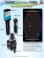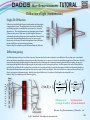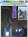
1
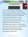
Ha a Ori II Ha He I M 42 Hb [O III] Hb Be Star g Cas Hg V3.5E © Bernd Koch | [email protected] 1 Contents Workshop on stellar spectroscopy at the college CFG Wuppertal DADOS & accessories DADOS layout Spectrum photography & visual guiding Optical path Dado #1, the ‘‘guiding port“: Slit plate, mirror and slit illuminator Dado #1: Field of view at the slit viewing port Dado #1: a CMa (Sirius) close to 25 mm Slit (DMK41 - video camera) Dado #1: Lunar Spectroscopy – The Aristarchus Plateau (DMK 41) Dado #2: The blazed reflection grating Daylight spectrum of 900 lines/mm grating and 1200 lines/mm grating Dado #2: Grating replacement – Part 1 to 4 Diffraction of light (transmission) Transmission grating Blazed transmission grating vs. blazed reflection grating Blazed reflection grating Blazed grating theory: Definition of parameters Blazed grating theory Calculation example: DADOS with blazed 200 lines/mm grating Energy saving lamp ORMALIGHT 9W- DADOS with 200 lines/mm grating Spectrum of Energy Saving Lamp (ESL) Ormalight 9W V3.5E © Bernd Koch | [email protected] 4, 5 6 7 8 9 10 11, 12 13 14 15 16, 17 18-21 22 23 24 25 26 27, 28 29 30 31 2 Contents Stacking/calibration of stellar spectra Stacking/calibration of stellar spectra from a Canon DSLR camera The solar spectrum Calibration of Spectra with a Ne/Xe Plasma Tube from Conrad Electronic Nova Delphini 2013 Spectrum of Be star g Cas Spectrum of Be star z (zeta) Tau Spectroscopic binary star b Aur Emission nebula M42 Stacking & full calibration of spectra taken by a STF-8300M CCD camera References & recommended reading Safety and other rules Disclaimer V3.5E © Bernd Koch | [email protected] 32 33-86 87, 88 89-92 93-100 101-103 104-107 108, 109 110 111, 112 113, 114 115 116 3 Workshop on stellar spectroscopy at the college CFG Wuppertal The student astronomical observatory, on the roof of the college Carl-FuhlrottGymnasium, in Wuppertal, Germany, is well equipped with six identical telescope units. We provide astronomy and astrophysics education for larger groups of students from other colleges and the nearby Bergische Universitaet Wuppertal. Equipment: Astro-Physics 900GTO mount, Celestron 11‘‘ EdgeHD telescope, Pentax 75 SDHF refractor, Celestron ED 80/600mm refractor, Canon EOS 450D DSLR camera, SBIG STF-8300M CCD camera and lot of accessories. Special workshops on the topic of stellar spectroscopy are held with six units of the DADOS spectrograph. Gratings with 200/900/1200 lines/mm are available, as well as spectral calibration lamps. Tutors: Michael Winkhaus, Bernd Koch and Ernst Pollmann. Please look at the report of Dr. Thomas Schroefl of Vienna, Austria, who attended our October 21-25, 2013 workshop (all pages in German). http://www.waa.at/bericht/2013/10/20131021sfl00.html http://www.waa.at/bericht/2013/10/20131022sfl17.html If you are interested in a workshop, please have a look at our website www.schuelerlabor-astronomie.de or contact Mr. Michael Winkhaus, head of the observatory: [email protected] Michael Winkhaus Ernst Pollmann Please address inquiries about the DADOS spectrograph directly to Mr. Bernd Koch, [email protected] V3.5E © Bernd Koch | [email protected] Bernd Koch 4 Workshop on stellar spectroscopy at the college CFG Wuppertal Guiding Pentax 75 SDHF Camera Pentax 75 C11 EdgeHD DADOS Lage des Spalts unbekannt Credit: Bernd Koch Spectrum recording Guiding Controller Interested in a workshop? Please contact: Michael Winkhaus, [email protected] | Workshop April, 2011 V3.5E © Bernd Koch | [email protected] 5 DADOS & accessories #2456313 T2 Quick changer #2456320 T2 Quick change ring Canon T2 Ring #1304110 Kellner 10 mm guiding eyepiece #1304120 Kellner 20mm positioning eyepiece #2958027 1 ¼‘‘ Stop Ring # 2458556 Blaze reflection grating 900 lines/mm Slit Viewer #2458550 DADOS slit spectrograph #2458590 Neon calibration lamp #2452110 Carrying case for DADOS and accessories V3.5E © Bernd Koch | [email protected] 6 DADOS layout 1) 2" Nosepiece ( -> Telescope) 2) Adjustable red LED slit illuminator (incl. two 1.5V LR-41 batteries) 3) 1¼" Slit viewer port for guiding eyepiece (11) or camera 4) 1¼" Stop ring for guiding eyepiece (11) or camera 5) Micrometer adjustment for scanning the spectrum 6) Rotation stage counter spring (do not touch) 7) Focuser 8) Focuser locking screws 9) Grating angle locking screw 10) Optional 900 lines/mm grating 11) Guiding eyepiece for viewing the spectrograph‘s slit 12) Quick changer (optional, but not for DSLR) 13) Focusing eyepiece holder, T2 -> 1¼" 14) 10 mm or 20 mm Kellner eyepieces for viewing a spectrum) V3.5E © Bernd Koch | [email protected] 7 Spectrum photography & visual guiding ‘‘Los dados“ – The cubes (Spanish) 2‘‘ Nosepiece Telescope El dado 1 (slit plate) Allen wrenches Adjustable red LED slit illuminator T2 ring Slit viewer assembly Guiding eyepiece (to keep object on slit) El dado 2 (grating) Micrometer adjustment (spectrum scanning) V3.5E © Bernd Koch | [email protected] Focus lock Focuser Grating angle locking screw (please loosen this screw before turning the micrometer adjustment!) 8 Optical path Collimator Slit Grating Mirror Objective Focal plane V3.5E © Bernd Koch | [email protected] 9 Dado #1, the ‘‘guiding port“: Slit plate, mirror and slit illuminator Slit viewing port (guiding port) Slit plate: The slit plate contains three slits of different widths: 25 mm, 35 mm, and 50 mm. Mirror: The small mirror allows the observer at the slit viewing port to keep an object‘s image exactly on one the slits. Slit plate Mirror Slit illuminator Slit illuminator: To be visible against a dark sky background, the slits can be illuminated by an adjustable red LED. Please note: Don‘t forget to switch off the slit illuminator before starting the exposure of the spectrum. Otherwise the red LED stray light will be superimposed on the image of the spectrum. To save battery energy always be sure to switch off the illuminator while not in use. The illuminator holds two 1.5V batteries LR41. V3.5E © Bernd Koch | [email protected] 10 Dado #1: Field of view at the slit viewing port Guiding camera Guiding eyepiece Slit viewer Slit viewer Slit viewing port 2‘‘ Nosepiece Slit plate Mirror Slit illuminator Point the 2‘‘ nosepiece at a bright light source Look through the guiding eyepiece Each of the three slits has a different width The width of a slit is crucial for spectral resolution The length of a slit is irrelevant V3.5E © Bernd Koch | [email protected] 11 Dado #1: Field of view at slit viewing port Guiding camera Guiding eyepiece Slit viewer Slit viewer d Slit viewing port 2‘‘ Nosepiece • • • • • Slit illuminator • Slit plate Mirror a Central slit (25 mm) gives best spectral resolution The 50 mm slit provides the brightest visual stellar spectra Spectral resolution is independent of the telescope‘s focus Perfect telescope focus maximizes contrast of spectral lines Guiding is possible at the slit viewing port The slit‘s length should be parallel to Declination d direction V3.5E © Bernd Koch | [email protected] 12 Dado #1: a CMa (Sirius) close to 25 mm Slit (DMK41 - video camera) Nachführokular Video: Bernd Koch Slit-Viewer V3.5E © Bernd Koch | [email protected] 13 Video: Jonas Niepmann / Laurenz Sentis / Bernd Koch Dado #1: Lunar Spectroscopy – The Aristarchus Plateau (DMK 41) V3.5E © Bernd Koch | [email protected] 14 Credit: DADOS Spectrograph User Manual Dado #2: The blazed reflection grating To avoid damage, please change the grating strictly according to DADOS user manual. Also be careful with the tiny set screws and don‘t touch the optical surface of the grating !!!! Two blazed reflection gratings are recommended by the designers of the DADOS spectrograph: Low resolution 200 lines/mm, linear dispersion 2.16 Å/px (0.2 nm/px) @ 6563 Å / 5.4 micron pixel Medium resolution 900 lines/mm, linear dispersion 0,59 Å/px (0.059 nm/px) Optional: High resolution 1200 lines/mm, linear dispersion 0.46 Å/px (0.046 nm/px) A modified DSLR Camera with an 18 mm x 22 mm APS-size sensor covers the whole spectrum (about 400 nm – 700 nm) only if used with the 200 lines/mm grating. The camera field should be aligned parallel to the spectrum to minimize aliasing errors due to rotation of the spectrum. This can be achieved by loosening three set screws at the T2-adapter, rotating the inner T2-ring, and tightening the set screws. V3.5E © Bernd Koch | [email protected] 15 Daylight spectrum of 900 l/mm grating and 1200 l/mm grating Mg Triplet EOS 10D, 900 lines/mm, exposure: 1 s unprocessed unsharp masking EOS 1000D, 1200 lines/mm, exposure: 5 s 900 lines/mm Exposure: 1 s Unsharp masking 1200 lines/mm Exposure: 5 s Dl = 1,6Å fully resolved V3.5E © Bernd Koch | [email protected] Unsharp masking 16 www.lightfrominfinity.org /HIRSS/HIRRS.htm Daylight spectrum of 900 lines/mm grating and 1200 lines/mm grating V3.5E © Bernd Koch | [email protected] 17 Dado #2: Grating replacement – Part 1 V3.5E © Bernd Koch | [email protected] 18 Dado #2: Grating replacement – Part 2 V3.5E © Bernd Koch | [email protected] 19 Dado #2: Grating replacement – Part 3 V3.5E © Bernd Koch | [email protected] 20 Dado #2: Grating replacement – Part 4 Copyright: DADOS Spectrograph‘s User‘s Manual by Baader Planetarium GmbH V3.5E © Bernd Koch | [email protected] 21 Diffraction of light (transmission) Single-Slit Diffraction Diffraction is described by the Huygens–Fresnel principle and the principle of superposition of waves. The propagation of a wave can be visualized by considering every point on a wavefront as a point source for a secondary spherical wave. The wave displacement at any subsequent point is the sum of these secondary waves. When waves are added together, their sum is determined by the relative phases as well as the amplitudes of the individual waves so that the summed amplitude of the waves can have any value between zero and the sum of the individual amplitudes. Hence, diffraction patterns usually have a series of maxima and minima. Reference: http://en.wikipedia.org/wiki/Diffraction#Single-slit_diffraction Diffraction grating An idealized grating is made up of a set of slits of spacing d, that must be wider than the wavelength to cause diffraction. When a plane wave of wavelength λ with normal incidence perpendicular to the grating, each slit in the grating acts as a quasi point-source from which light propagates in all directions. After light interacts with the grating, the diffracted light is composed of the sum of interfering wave components emanating from each slit in the grating. At any given point in space through which diffracted light may pass, the path length to each slit in the grating will vary. So will the phases of the waves at that point from each of the slits, and thus will add or subtract from one another to create peaks and valleys, through the phenomenon of additive and destructive interference. When the path difference between the light from adjacent slits is equal to half the wavelength λ/2, the waves will all be out of phase, and thus will cancel each other to create points of minimum intensity. Similarly, when the path difference is λ, the phases will add together and maxima will occur. Reference: http://en.wikipedia.org/wiki/Diffraction_grating 2 ∙ ( 2 ( ( ( 𝐼(sin 𝛽) = 𝐼0 𝜋𝑏 sin( sin 𝛽) 𝜆 𝜋𝑏 sin 𝛽 𝜆 𝑁𝜋𝑑 sin( sin 𝛽) 𝜆 𝜋𝑑 sin 𝛽 𝜆 Diffraction term Interference term of a slingle slit width b of N slits at distance d Reference: N05_Monochromatoren_d_BAneu.doc - 2/21 V3.5E © Bernd Koch | [email protected] 22 Transmission grating Zero order First order Second order Third order Intensity First order Maximum intensity in zero order Disadvantages of a transmission grating Light is dispersed among the various diffraction orders, leading to low intensity in the higher ones. Transmission losses are due to selective absorption in the glass. Maximum intensity is the undiffracted zeroth order. A blazed transmission grating will improve things. V3.5E © Bernd Koch | [email protected] 23 Blazed transmission grating vs. blazed reflection grating • Reflection gratings can be used in spectral regions where glass substrates and resins absorb light (e.g., the ultraviolet). • Reflection gratings provide much higher resolving power than equivalent transmission gratings, since the path difference between neighboring beams (i.e., separated by a single groove) is higher in the case of the reflection grating. Therefore transmission gratings must be wider (so that more grooves are illuminated) to obtain comparable resolving power. • Reflection grating systems are generally smaller than transmission grating systems, because the reflection grating acts as a folding mirror. V3.5E © Bernd Koch | [email protected] http://gratings.newport.com/information/handbook/chapter12.asp#12.2 Although in some cases transmission gratings are applicable or even desirable, they are not often used. Reflection gratings are much more prevalent in spectroscopic and laser systems, due primarily to the following advantages: 24 Blazed reflection grating Zero order First order Zero Order First Order Second order Third order Intensity First order Advantages The highest efficiency is in first order with the correct blaze angle. The reflectivity is higher than the throughput of a blazed transmission grating . V3.5E © Bernd Koch | [email protected] 25 Blazed grating theory: Definition of parameters GN: Grating normal FN: Face normal g: Groove spacing f: Blaze angle a: Angle of the incident light b: Angle of reflected light V3.5E © Bernd Koch | [email protected] 26 Blazed grating theory GN: Grating normal FN: Face normal g: Groove spacing f: Blaze angle a: Angle of the incident light f b: Angle of reflected light S1 S2 Additive interference occurs when the total path difference D of light from adjacent slits (S1) and (S2) is an integer multiple of the wavelength λ: The phase is then the same, so the beams’ intensity add. Path difference of incident beam: D1 = BA' = g sin a, Path difference of reflected beam: D2 = AC = g sin b D = m l = D1 – D2 = g (sin a - sin b) with m =0, ± 1, ± 2 ... (Grating equation) V3.5E © Bernd Koch | [email protected] 27 Blazed grating theory f GN: Grating normal FN: Face normal g: Groove spacing f: Blaze angle a: Angle of the incident light b: Angle of reflected light f Grating equation: Derivative with respect to b: Angular dispersion: Linear dispersion: ‘‘f“ is the focal length of the objective lens Blaze angle: V3.5E © Bernd Koch | [email protected] 28 Calculation example: DADOS with blazed 200 lines/mm grating Data Entry: Celestron C11 Telescope aperture: 280 𝑚𝑚 Telescope focal length: 2800 𝑚𝑚 Grating groove density: 200 𝑙𝑖𝑛𝑒𝑠/𝑚𝑚 1 Groove spacing 𝑔 = 200 𝑚𝑚 Total deflection angle: 𝛼 + 𝛽 = 90° Central wavelength: 𝜆 = 520 𝑛𝑚 = 5200 Å Diffraction order : 𝑚 = 1 Slit width: 25 mm Camera: Canon EOS 450D SimSpec Results: Angle of incident light: 𝛼 = 49.22° Angle of reflected light: |𝛽| = 40.78° Dispersion: 2.05 Å/px Spectral resolution: 13.62 Å at 5200 Å Resolving power: 382 Blaze angle: 𝜑 = 4.22° = 4° 13′ Linear dispersion: 394.37 Å/mm Length of the spectrum: ca. 8 mm http://www.astrosurf.com/buil/us/compute/SimSpec_V4_0.xls V3.5E © Bernd Koch | [email protected] 29 Energy saving lamp ORMALIGHT 9W - DADOS with 200 lines/mm grating m: -1 0 1 2 3 Highest efficiency 1st Order m = 1 is most efficient. Can be used for stellar spectroscopy from 3500 Å to about 10,000 Å with an ultraviolet and infrared sensitive CCD camera. In that case be careful: 1st order in the infrared beyond 8500 Å overlaps the 2nd order! You may check this by taking the sun‘s spectrum (daylight spectrum) with your camera. A DSLR camera modified with a Baader UV/IR cut filter is only sensitive between roughly 4000 Å and 700o Å. Higher Orders than the first can be used for spectroscopy only in a smaller wavelength range. But the higher spectral resolution is bought dearly due to low efficiency. A grating with 900 lines/mm or 1200 lines/mm is recommended to achieve higher spectral resolution. V3.5E © Bernd Koch | [email protected] 30 V3.5E © Bernd Koch | [email protected] 31 Stacking/calibration of stellar spectra Stacking & calibration of spectra obtained with a DSLR camera + If you already have a DSLR camera, please practice with it by recording a daylight spectrum (= solar spectrum, G2V) + Cheaper than any CCD camera with a similar ‘‘big“ sensor (APS-C) + Easier handling than a CCD camera + LiveView mode for easy focusing at a bright light source, e.g. ESL + You can easily find your way through the spectrum (red/blue) + Easy identification of spectral features due to color + Autodark improves SNR at the cost of exposure time - Low signal-to-noise ratio images - Low sensitivity at less than 4000Å means the Ca II lines are barely visible - Non-modified DSLRs have low sensitivity above 6000Å Stacking & calibration of spectra obtained with a cooled b&w CCD camera + Sensitive from about 3500Å (‘‘Balmer Jump“ at 3646Å) to about 10000Å (IR) + High signal-to-noise ratio images + Separate dark frames useful (dark frame library) + No need for a color camera: Synthetic color spectra can be created with Vspec - Difficult to handle for beginners in astrophotography and astrospectroscopy V3.5E © Bernd Koch | [email protected] 32 Stacking/calibration of stellar spectra from a Canon DSLR camera Ha ca. 98% Baader BCF filter Credit: Bernd Koch, Axel Martin Canon filter ca. 25% http://www.baader-planetarium.de/sektion/s45/canon_astroupgrade-english.htm V3.5E © Bernd Koch | [email protected] 33 Stacking/calibration of stellar spectra from a Canon DSLR camera Exercise 1: a Orionis (Betelgeuse) a Date 2010-12-15 Pentax 75 SDHF / 500mm Canon EOS 450D (Baader BCF-Filter) ISO 800 Spectrograph: DADOS Grating: 200 l/mm Spectral resolution: 12 Å @5500 Å Scale: 2.1 Å/Pixel Betelgeuse: Spectral Class M2Iab Apparent magnitude: 0.7 mag Set of 11 spectra, each 8 s exposed Darkframes: not used Flatflields: not used Images: …/Betelgeuse_200L_2010-12-15/ 1 x 8s 11 x 8s V3.5E © Bernd Koch | [email protected] 34 Stacking/calibration of stellar spectra from a Canon DSLR camera a Orionis (Betelgeuse), M2Iab 1 x 8s 11 x 8s DADOS 200 lines/mm, Canon EOS 450D (BCF filter) 1x8s 11 x 8 s Improved SNR (signal-to-noise ratio) due to stacking V3.5E © Bernd Koch | [email protected] 35 Stacking/calibration of stellar spectra from a Canon DSLR camera Step 1: Image Browser - Check the quality of spectral images Step 2: Fitswork - Download and check settings Step 3: Fitswork – The stacking process: Create an averaged color spectrum Step 4: Fitswork – Rotate, crop, convert to monochrome spectrum & save Step 5: Visual Spec (VSpec) – Spectrum calibration (w/o instrumental response) Step 6: Visual Spec (VSpec) - Visualize Profile as synthetic (color) profile Step 7: VisualSpec (VSpec) – Spectrum calibration by instrumental response and calculation of the effective temperature of Betelgeuse from its spectrum Step 8: Visual Spec (VSpec) - Visualize profile as a synthetic (color) profile V3.5E © Bernd Koch | [email protected] 36 Stacking/calibration of stellar spectra from a Canon DSLR camera Step 1: Check the quality of spectral images in an image browser Dataset: …/Betelgeuse_200L_2010-12-15/1_Spectra_JPG/ Note the image numbers of the perfectly imaged spectra with regard to exposure time and sharpness of spectral features. Ignore imperfect spectra! V3.5E © Bernd Koch | [email protected] 37 Stacking/calibration of stellar spectra from a Canon DSLR camera Step 2: Spectrum stacking with Fitswork • Download Fitswork at http://www.fitswork.de/software/softw_en.php • Start Fitswork V3.5E © Bernd Koch | [email protected] 38 Stacking/calibration of stellar spectra from a Canon DSLR camera Step 2: Spectrum stacking with Fitswork Settings V3.5E © Bernd Koch | [email protected] 39 Stacking/calibration of stellar spectra from a Canon DSLR camera Step 3: Fitswork – The stacking process: Create an averaged color spectrum Dataset: …/Betelgeuse_200L_2010-12-15/2_Spectra_raw_images_CR2 File Batch Processing V3.5E © Bernd Koch | [email protected] 40 Stacking/calibration of stellar spectra from a Canon DSLR camera Step 3: Fitswork – The stacking process: Create an averaged color spectrum Dataset: …/Betelgeuse_200L_2010-12-15/2_Spectra_raw_images_CR2 1. Step of Processing [sic] 1 2 1. File Select first raw image file 2. All files in folder 3. Press right arrow button to proceed 3 V3.5E © Bernd Koch | [email protected] 41 Stacking/calibration of stellar spectra from a Canon DSLR camera Step 3: Fitswork – The stacking process: Create an averaged color spectrum Dataset: …/Betelgeuse_200L_2010-12-15/2_Spectra_raw_images_CR2 2. Step of Processing [sic] Add to destination image Planet/Moon Crosscorrelation Number of Marks Function: Mid. (means average) Press start button V3.5E © Bernd Koch | [email protected] 42 Stacking/calibration of stellar spectra from a Canon DSLR camera Step 3: Fitswork – The stacking process: Create an averaged color spectrum Dataset: …/Betelgeuse_200L_2010-12-15/2_Spectra_raw_images_CR2 1. 2. 3. 4. 5. 6. 7. 8. Draw a tight yellow frame around the first spectrum Skip bad images which are not properly focused or exposed Load the next frame (‘‘Ok, go on“) Check if the area is marked (yellow frame is still in place) Go through all images with or without controlling image quality The final image, the stacked spectrum, will be saved after a while as ‘‘Result_image.fit“ Create a new folder ‘‘3_Results‘‘ and save copy of ‘‘Result_image.fit‘‘ ‘‘3_Results‘‘ is your new working directory Please note! The quality of the final spectrum depends on recognizing spectral lines in each single image. Spectra with short exposure times, and consequently low contrast, may not stack properly. V3.5E © Bernd Koch | [email protected] 43 Stacking/calibration of stellar spectra from a Canon DSLR camera Step 4: Fitswork - Rotate and save again as ‘‘Result_image.fit“ Rotate ‘‘Result_image.fit‘‘ to achieve a perfectly leveled spectrum Processing Image Geometry Rotate image with Subsidiary Line V3.5E © Bernd Koch | [email protected] 44 Stacking/calibration of stellar spectra from a Canon DSLR camera Step 4: Fitswork - Rotate ‘‘Result_image.fit‘‘ perfectly leveled spectrum • • Please mark a line exactly along the spectrum with the left mouse button then Ok Whole Image V3.5E © Bernd Koch | [email protected] 45 Stacking/calibration of stellar spectra from a Canon DSLR camera Step 4: Fitswork – Crop & save Draw a yellow frame around the spectrum Cut off Save as ‘‘Result_image_color_16bit.fit‘‘ V3.5E © Bernd Koch | [email protected] 46 Stacking/calibration of stellar spectra from a Canon DSLR camera Step 4: Fitswork – Convert to black & white image and save Processing Color image to b/w (luminance) Save as ‘‘Result_image_mono_16bit‘‘ V3.5E © Bernd Koch | [email protected] 47 Stacking/calibration of stellar spectra from a Canon DSLR camera Step 5: VisualSpec (VSpec) – Spectrum calibration VSpec Software Download: http://valerie.desnoux.free.fr/ Please note: VisualSpec accepts monochrome 16 bit files only V3.5E © Bernd Koch | [email protected] 48 Stacking/calibration of stellar spectra from a Canon DSLR camera Step 5: VisualSpec (VSpec) – Spectrum calibration without correction for the instrumental profile Betelgeuse: Result_image_mono_16bit Create a spectrum profile Identify spectral lines Calibrate wavelength Raw profile Divide a continuum profile, which was extracted from the raw profile Continuum Normalize intensity to ‘‘1“. Measure Doppler shifts or Equivalent Widths (EW) of lines Spectrum profile normalized to ‘‘1‘‘ V3.5E © Bernd Koch | [email protected] 49 Stacking/calibration of stellar spectra from a Canon DSLR camera Step 5: VisualSpec (VSpec) - Preferences 5.1 Open VSpec 5.2 Options Preferences Working directory ‘‘3_Results‘‘ Image .fits and Profile .spc 5.3 File Open image: ‘‘Result_image_mono_16bit.fit‘‘ V3.5E © Bernd Koch | [email protected] 50 Stacking/calibration of stellar spectra from a Canon DSLR camera Step 5: VisualSpec (VSpec) – Create a spectrum profile 5.4 Profile extraction All set to ‘‘Auto‘‘ OK Close V3.5E © Bernd Koch | [email protected] 51 Stacking/calibration of stellar spectra from a Canon DSLR camera Step 5: VisualSpec (VSpec) – Save the spectrum profile 5.5 Press to display pixel positions and intensity The result is a spectrum profile with (x,y) = (pixel positions, intensity). ‘‘Tilt“: Spectrum is not perfectly leveled (angle -0.01°), so the spectral lines are not perfectly perpendicular. This has no measurable effect on the calibration. 5.6 Save ‘‘Result_image_16bit.spc‘‘ Due to a different stacking procedure and color conversion, the spectrum intensities on the following pages differ somehow. This has no effect on the final profile as it is being calibrated (continuum removed or instrumental profile used). Pixel V3.5E © Bernd Koch | [email protected] 52 Stacking/calibration of stellar spectra from a Canon DSLR camera Step 5: Visual Spec (VSpec) – Identification of spectral features 5.7 Print the raw profile and note the wavelengths of precisely known spectral lines of a star of similar class a Ori (Betelgeuse, Class M2Iab) telluric l/Å Suggested reference: Spectroscopic Atlas for Amateur Astronomers, by Swiss amateur astronomer Richard Walker http://www.ursusmajor.ch/downloads/spectroscopic-atlas-4.0.pdf V3.5E © Bernd Koch | [email protected] 53 Stacking/calibration of stellar spectra from a Canon DSLR camera Step 5: Visual Spec (VSpec) – From pixel to Ångstrom: Wavelength calibration of the x-axis 5.8 Calibration multiple line 6 5.9 Save as ‘‘Result_image_wavecal.spc‘‘ a Ori (Betelgeuse, Class M2Iab) V3.5E © Bernd Koch | [email protected] telluric 54 Stacking/calibration of stellar spectra from a Canon DSLR camera Step 5: Visual Spec (VSpec) – Continuum extraction from the raw profile 5.10 Compute continuum a Ori (Betelgeuse, Class M2Iab) l/Å V3.5E © Bernd Koch | [email protected] 55 Stacking/calibration of stellar spectra from a Canon DSLR camera Step 5: Visual Spec (VSpec) – Continuum extraction from the raw profile 5.11 Press ‘‘point/courbe[sic]‘‘: set 20 to 50 points (actually green crosses) along the continuum (upper limit) + + + + + a Ori (Betelgeuse, Class M2Iab) + + + + + + + + + + + + + + + + + + + + + + + + + + + + + + + + + + + V3.5E © Bernd Koch | [email protected] l/Å + + 56 Stacking/calibration of stellar spectra from a Canon DSLR camera Step 5: Visual Spec (VSpec) – Continuum extraction from the raw profile 5.12 Press ‘‘Execute‘‘. The resulting continuum is the orange-red line a Ori (Betelgeuse, Class M2Iab) l/Å V3.5E © Bernd Koch | [email protected] 57 Stacking/calibration of stellar spectra from a Canon DSLR camera Step 5: Visual Spec (VSpec) – Continuum extraction from the raw profile 5.13 Edit Replace Intensity V3.5E © Bernd Koch | [email protected] 58 Stacking/calibration of stellar spectra from a Canon DSLR camera Step 5: Visual Spec (VSpec) – Continuum extraction from the raw profile 5.14 Save as Continuum.spc l/Å V3.5E © Bernd Koch | [email protected] 59 Stacking/calibration of stellar spectra from a Canon DSLR camera Step 5: Visual Spec (VSpec) – Continuum division 5.15 File Open profile Continuum.spc and ‘‘Result_image_wavecal.spc‘‘ 5.16 Highlight the window ‘‘Result_image_wavecal.spc‘‘ V3.5E © Bernd Koch | [email protected] 60 Stacking/calibration of stellar spectra from a Canon DSLR camera Step 5: Visual Spec (VSpec) – Continuum division 5.17 Operations Divide profile by profile Click on: continuum.spc intensity V3.5E © Bernd Koch | [email protected] 61 Stacking/calibration of stellar spectra from a Canon DSLR camera Step 5: Visual Spec (VSpec) – Continuum division 5.18 The ‘‘green profile‘‘ is the result of division. Now, prepare to save the result: a Ori (Betelgeuse, Class M2Iab) V3.5E © Bernd Koch | [email protected] l/Å 62 Stacking/calibration of stellar spectra from a Canon DSLR camera Step 5: Visual Spec (VSpec) – The normalized profile of Betelgeuse 5.19 Edit Replace Intensity 5.20 Save as ‘‘Result_image_wavecal_normalized.spc‘‘ a Ori (Betelgeuse, Class M2Iab) l/Å V3.5E © Bernd Koch | [email protected] 63 Stacking/calibration of stellar spectra from a Canon DSLR camera Step 5: Visual Spec (VSpec) – The normalized profile of Betelgeuse 5.21 Indicate middle area with left mouse button to become ‘‘1“ in intensity 5.22 Press button ‘‘Normalize‘‘ a Ori (Betelgeuse, Class M2Iab) l/Å V3.5E © Bernd Koch | [email protected] 64 Stacking/calibration of stellar spectra from a Canon DSLR camera Step 5: Visual Spec (VSpec) – The normalized profile of Betelgeuse 5.23 Result: Wavelength calibrated and intensity normalized profile of Betelgeuse 5.24 Save as ‘‘Result_image_wavecal_normalized to 1.spc‘‘ a Ori (Betelgeuse, Class M2Iab) 1 l/Å 0 V3.5E © Bernd Koch | [email protected] 65 Stacking/calibration of stellar spectra from a Canon DSLR camera Step 5: Visual Spec (VSpec): Calibration summary Raw profile Wavelength calibrated Pseudo continuum (to be divided) Normalization to ‘‘1‘‘ Final result, but not corrected for the instrumental profile a Ori (Betelgeuse, Class M2Iab) V3.5E © Bernd Koch | [email protected] 66 Stacking/calibration of stellar spectra from a Canon DSLR camera Step 6: Visual Spec (VSpec) - Visualize profile as synthetic profile 6.1 Tools Synthese[sic]: Creates a synthetic black & white spectrum a Ori (Betelgeuse, Class M2Iab) l/Å V3.5E © Bernd Koch | [email protected] 67 Stacking/calibration of stellar spectra from a Canon DSLR camera Step 6: Visual Spec (VSpec) - Visualize profile as synthetic profile 6.2 Synthese[sic] Colorer[sic]: creates a colored synthetic spectrum a Ori (Betelgeuse, Class M2Iab) Hb Mg Triplet Na D V3.5E © Bernd Koch | [email protected] Ha l/Å 68 Stacking/calibration of stellar spectra from a Canon DSLR camera Comparison of spectral resolution of Betelgeuse spectra: DADOS 200 lines/mm and 900 lines/mm Hb Mg Triplet Na D 5890Å – 5896Å Na D well resolved V3.5E © Bernd Koch | [email protected] 200 lines/mm 900 lines/mm 69 Stacking/calibration of stellar spectra from a Canon DSLR camera Step 7: Visual Spec (VSpec) – Spectrum calibration by removing the instrumental profile Betelgeuse: Result_Image_mono_16bit Create a spectrum profile Identify spectral lines Calibrate wavelength Betelgeuse profile (M2Iab) Create the instrumental profile function via the use of a reference spectrum of the same spectral class Instrumental response Divide the Betelgeuse profile by instrumental profile function Final, calibrated spectrum profile V3.5E © Bernd Koch | [email protected] 70 Stacking/calibration of stellar spectra from a Canon DSLR camera Step 7: Visual Spec (VSpec) – Spectrum calibration by removing the instrumental profile 7.1 File Open profile ‘‘Result_image_wavecal.spc‘‘ a Ori (Betelgeuse, Class M2Iab) l/Å V3.5E © Bernd Koch | [email protected] 71 Stacking/calibration of stellar spectra from a Canon DSLR camera Step 7: Visual Spec (VSpec) – Spectrum calibration by removing the instrumental profile 7.2 Assistant Instrumental response [sic] assistant 7.3 Pickles Press on green arrow button Open ‘‘m2i.dat‘‘ (= Class M2I) V3.5E © Bernd Koch | [email protected] 72 Stacking/calibration of stellar spectra from a Canon DSLR camera Step 7: Visual Spec (VSpec) – Spectrum calibration by removing the instrumental profile The red profile is the reference spectrum of a star of similar spectral class l/Å V3.5E © Bernd Koch | [email protected] 73 Stacking/calibration of stellar spectra from a Canon DSLR camera Step 7: Visual Spec (VSpec) – Spectrum calibration by removing the instrumental profile 7.4 Press green arrow button ‘‘Division and extraction‘‘ Result: The orange profile is the (unsmoothed) instrumental profile l/Å V3.5E © Bernd Koch | [email protected] 74 Stacking/calibration of stellar spectra from a Canon DSLR camera Step 7: Visual Spec (VSpec) – Spectrum calibration by removing the instrumental profile 7.5 Smooth the instrumental profile. Press button ‘‘point/curve‘‘ and set about 60 ‘‘green crosses“ along the continuum a Ori (Betelgeuse, Class M2Iab) l/Å V3.5E © Bernd Koch | [email protected] 75 Stacking/calibration of stellar spectra from a Canon DSLR camera Step 7: Visual Spec (VSpec) – Spectrum calibration by removing the instrumental profile 7.6 Press button ‘‘OK‘‘ and press ‘‘execute‘‘ Flux a Ori (Betelgeuse, Class M2Iab) l/Å V3.5E © Bernd Koch | [email protected] 76 Stacking/calibration of stellar spectra from a Canon DSLR camera Step 7: Visual Spec (VSpec) – Spectrum calibration by removing the instrumental profile 7.7 Erase graphic Edit Replace: Intensity 7.8 File Save as ‘‘response.spc“ l/Å V3.5E © Bernd Koch | [email protected] 77 Stacking/calibration of stellar spectra from a Canon DSLR camera Step 7: Visual Spec (VSpec) – Spectrum calibration by removing the instrumental profile 7.9 While ‘‘response.spc“ is still open: File open profile ‘‘Result_image_wavecal.spc“ (please highlight) 7.10 Operations Divide profile by profile: Select ‘‘intensity“ (below response.spc) V3.5E © Bernd Koch | [email protected] 78 Stacking/calibration of stellar spectra from a Canon DSLR camera Step 7: Visual Spec (VSpec) – Spectrum calibration by removing the instrumental profile Result: The green profile is the calibrated, true spectrum profile of Betelgeuse, corrected for instrumental profile 7.11 Close ‘‘response.spc“ V3.5E © Bernd Koch | [email protected] 79 Stacking/calibration of stellar spectra from a Canon DSLR camera Step 7: Visual Spec (VSpec) – Spectrum calibration by removing the instrumental profile The green profile must be converted to a blue profile, before it can be saved 7.12 Erase graphic Edit Replace: Intensity 7.13 File Save as ‘‘Betelgeuse_final_spectrum.spc“ a Ori (Betelgeuse, Class M2Iab) l/Å V3.5E © Bernd Koch | [email protected] 80 Stacking/calibration of stellar spectra from a Canon DSLR camera Step 7: Visual Spec (VSpec) – Spectrum calibration by removing the instrumental profile 7.14 Use left mouse button and select area around 5500Å a Ori (Betelgeuse, Class M2Iab) l/Å V3.5E © Bernd Koch | [email protected] 81 Stacking/calibration of stellar spectra from a Canon DSLR camera Step 7: Visual Spec (VSpec) – Spectrum calibration by removing the instrumental profile 7.15 Normalize to 1: Press button ‘‘1‘‘ 7.16 File Save as ‘‘Betelgeuse_final_spectrum.spc“ a Ori (Betelgeuse, Class M2Iab) l/Å V3.5E © Bernd Koch | [email protected] 82 Stacking/calibration of stellar spectra from a Canon DSLR camera Step 7: Visual Spec (VSpec) – Using the spectrum to estimate temperature 7.17 Calculation of the effective temperature of Betelgeuse from its spectrum We assume thermal radiation of a black body according to Planck‘s Law. Radiometry Auto Planck (black line) http://en.wikipedia.org/wiki/File:Wiens_law.svg A Planck spectrum with 𝑇𝑒𝑓𝑓 =3000K (best fit) is fitted by VSpec: a Ori (Betelgeuse, Class M2Iab) V3.5E © Bernd Koch | [email protected] 83 Stacking/calibration of stellar spectra from a Canon DSLR camera Step 7: Visual Spec (VSpec) – Using the spectrum to estimate temperature 7.18 Wien‘s law 𝜆𝑚𝑎𝑥 29000 ∙ 103 Å ⋅ 𝐾 ≈ 𝑇𝑒𝑓𝑓 𝜆𝑚𝑎𝑥 : Wavelength of the maximum of the assumed black body emission 𝑇𝑒𝑓𝑓 : Effective Temperature [K] a Ori (Betelgeuse, Class M2Iab) VSpec result: 𝑇𝑒𝑓𝑓 =3000K (black line) 𝜆𝑚𝑎𝑥 =9700Å (officially adopted value 𝑇𝑒𝑓𝑓 =3450K) V3.5E © Bernd Koch | [email protected] 84 Stacking/calibration of stellar spectra from a Canon DSLR camera Step 8: Visual Spec (VSpec) - Visualize profile as synthetic profile 8.1 Synthese [sic] Creates a synthetic black & white spectrum a Ori (Betelgeuse, Class M2Iab) V3.5E © Bernd Koch | [email protected] 85 Stacking/calibration of stellar spectra from a Canon DSLR camera Step 8: Visual Spec (VSpec) - Visualize profile as synthetic profile 8.2 Synthese [sic] Colorer [sic] Creates a synthetic color spectrum for presentation a Ori (Betelgeuse, Class M2Iab) V3.5E © Bernd Koch | [email protected] 86 The solar spectrum l/Å EOS 450D (Baader BCF filter) DADOS 900 lines/mm and DSLR camera Canon EOS 450Da (BCF). Paper by Tom Schnee and Johannes Schnepp (CFG Wuppertal, 2012) V3.5E © Bernd Koch | [email protected] 87 The solar spectrum ALccd 5.2 CCD Camera l/Å DADOS 900 lines/mm and ALccd 5.2 CCD camera. Paper by students Tom Schnee and Johannes Schnepp (CFG Wuppertal, 2012) V3.5E © Bernd Koch | [email protected] 88 Calibration of spectra with a Ne/Xe plasma tube from Conrad Electronic Credit: Dr. Thomas Schröfl Student astronomical observatory at CFG College in Wuppertal/Germany V3.5E © Bernd Koch | [email protected] 89 Calibration of spectra with a Ne/Xe plasma tube from Conrad Electronic V3.5E © Bernd Koch | [email protected] 90 Calibration of spectra with a Ne/Xe plasma tube from Conrad Electronic V3.5E © Bernd Koch | [email protected] 91 Calibration of spectra with a Ne/Xe plasma tube from Conrad Electronic V3.5E © Bernd Koch | [email protected] 92 Nova Delphini 2013: Discovery August 14.8174 UT http://en.wikipedia.org/wiki/Nova_Delphini_2013 V3.5E © Bernd Koch | [email protected] 93 Nova Delphini 2013: August 16, 2013 2013-08-16 | 23.22 UT – 23.55 UT | mid Exposure August 16.985 UT | 0.3m aperture, f/7.8 f=2340mm | SBIG ST-8300M | Baader RGB Filter | Nova maximum: Aug. 16.45 @ V=4.3 mag Image & Processing: Bernd Koch, Sorth/Germany V3.5E © Bernd Koch | [email protected] 94 Nova Delphini 2013: 2013-09-05.9 UT Spectrum: DADOS 200 lines/mm & SBIG ST-8300M CCD camera | 0.3m Telescope V3.5E © Bernd Koch | [email protected] 95 Nova Delphini 2013: 2013-09-05.9 UT Calibration with a Ne/Xe plasma tube from Conrad Electronic Spectrum: DADOS 200 lines/mm & SBIG ST-8300M CCD camera | 0.3m Telescope Ne/Xe plasma tube in front of the telescope, and spectrum superimposed during exposure. Note the changes in spectral resolution due to the different slit widths. V3.5E © Bernd Koch | [email protected] 96 Nova Delphini 2013-09-05.88785 UT Calibration with a Ne/Xe plasma tube from Conrad Electronic V3.5E © Bernd Koch | [email protected] 97 P Cygni Profile 2013-08-19 | 20.01 UT – 20.33 UT | Mid-exposure: August 19.84722 UT | DADOS 200 lines/mm Stacking: FITSWORK with 9 x 120s | Calibration: VisualSpec The expansion velocity 𝑣𝑟 of the nova‘s envelope is calculated by the P Cygni profile method, measured at Ha: ∆𝜆 𝑘𝑚 𝑣𝑟 = 𝑐 = 1005 𝜆0 0 𝑠 Δ𝜆 = 22.0Å, 𝜆0 = 6562.82Å, 𝑐0 = 299792 𝑘𝑚 𝑠 Ref.: www.ursusmajor.ch/downloads/analysis-andinterpretation-of-astronomical-sp.pdf V3.5E © Bernd Koch | [email protected] 98 P Cygni Profile 2013-08-19 | 20.01 UT – 20.33 UT | Mid-exposure: August 19.84722 UT| DADOS 200 lines/mm Stacking: FITSWORK with 9 x 120s | Calibration: VisualSpec The expansion velocity 𝑣𝑟 of the nova‘s envelope can also be calculated by the broadening of the emission lines, measured at Ha: 𝑣𝑟 ≈ 𝐹𝑊𝐻𝑀 𝑘𝑚 𝑐0 = 1220 𝜆0 𝑠 𝐹𝑊𝐻𝑀 = 26.7Å, 𝜆0 = 6562.82Å, 𝑐0 = 299792 𝑘𝑚 𝑠 Ref.: www.ursusmajor.ch/downloads/analysis-andinterpretation-of-astronomical-sp.pdf V3.5E © Bernd Koch | [email protected] 99 Nova Delphini 2013-08-19/23 & 2013-09-05 summary All spectra taken with DADOS 200 lines/mm with 0.3m Telescope by Bernd Koch Nova Delphini database: www.astrosurf.com/aras/novae/Nova2013Del.html V3.5E © Bernd Koch | [email protected] 100 Spectroscopy of Be star g Cas • • • Celestron 11 + DADOS 900 lines/mm + STF-8300M CCD camera Pentax 75 + 2x-Converter + DADOS 900 l/mm + STF-8300M CCD camera Spectrum recording & video camera guiding: MaxIm DL, Win XP/7 32-bit tested Set g Cas on the middle of the three slits (25 mm) for highest resolution The slit‘s length should be parallel to Deklination (d) direction Center spectrum on Ha by turning the micrometer adjustment Keep exposure time well below the saturation level of the sensor (1s … 60s) Guiding: Video camera Skyris 274M / TIS DMK 41 or else Number of images per spectrum: Minimum 20. Save in folder: ‘‘gamma Cas‘‘ Expose 20 darks of same exposure time and sensor temperature: Folder: ‘‘darks‘‘ Optional: Flat fields with auto darksubtraction. Folder: „flats“ Dark/Flat calibration with MaxIm DL, stacking with FITSWORK Spectrum calibration with Visual Spec (VSpec). V3.5E © Bernd Koch | [email protected] 101 Credit: Gemini Observatory Illustration by Jon Lomberg Ha Hb • • • Ha Celestron 11 + DADOS 900/200 lines/mm + EOS 450D (ISO 800, Autodark) Pentax 75 + 2x-Converter + DADOS 900/200 lines/mm + EOS 450D (ISO 800) Spectrum recording & video camera guiding: MaxIm DL, Win XP/7 32-bit tested The slit‘s length should be parallel to Deklination (d) direction Center spectrum on Ha or Hb by turning the micrometer adjustment Keep exposure time well below saturation of sensor (1s to about 60s) Guiding: Video camera Skyris 274M / TIS DMK 41 or else Number of images per spectrum: Minimum 20. Save in folder: ‘‘gamma Cas‘‘ Stacking with FITSWORK Spectrum calibration with Visual Spec (VSpec) Hb Ha V3.5E © Bernd Koch | [email protected] 102 Credit: Gemini Observatory Illustration by Jon Lomberg Spectroscopy of Be star g Cas http://en.wikipedia.org/wiki/Gamma_Cas Calibration with telluric H2O lines Ha Telluric lines H2O Telluric lines H2O Date: 2011-04-19.882 UT | C11 EdgeHD (0.28m aperture, f/10). DADOS 900 lines/mm grating. CCD camera Alccd 5.2 (QHY6). Single exposure: 120s. Average of 20 exposures. Darkframe subtraction, no flatfielding. Spectral resolution 2.3 Å at 6563Å. Calibration with VisualSpec (telluric H2O). FWHM=7.9Å, EW=-23.4Å (6520Å-6605Å), RV=-5.2 km/s. Spectrum obtained at a spectroscopy workshop at the College CFG Wuppertal/Germany. Calibration & results: Bernd Koch V3.5E © Bernd Koch | [email protected] 103 Credit: Gemini Observatory Illustration by Jon Lomberg Spectrum of Be star g Cas Spectrum of Be star z Tau Ha Ne I 6506.5277Å Ne I 6598.9528Å Ne I 6532.8824Å Date: 2014-03-10, mid-exposure 23.30 UT| 0.3m aperture, f/10. DADOS 1200 lines/mm grating. CCD camera SBIG ST-8300M, total exposure 3x300s with darkframe subtraction, without flatfielding. Spectral resolution about 1.49 Å. Calibration with Xenon/Neon plasma tube and VisualSpec software. Image processing & spectrum calibration: Bernd Koch V3.5E © Bernd Koch | [email protected] 104 Spectrum calibration VisualSpec DADOS 1200 lines/mm SBIG ST-8300M, 1 x 1 Binning Ha intensity in the red (R) and violet wing (V) of the Ha line Ne I 6506.5277Å Ne I 6532.8824Å Ne I 6598.9528Å V R Date: 2014-03-10, JD 2456727.386 | Spectral resolution: 1.5Å | Radial velocity v=30.9 km/s EW=-3.9Å (6540Å-6590Å) | V/R=1.00 | by Bernd Koch and Ernst Pollmann V3.5E © Bernd Koch | [email protected] 105 Credit: Gemini Observatory Illustration by Jon Lomberg Spectrum of Be star z Tau Credit: Ernst Pollmann V to R monitoring Multi-epoch Near-Infrared Interferometry of the Spatially Resolved Disk Around the Be Star ζ Tau (Schaefer et al., http://arxiv.org/abs/1009.5425) V3.5E © Bernd Koch | [email protected] 106 Credit: Gemini Observatory Illustration by Jon Lomberg Spectrum of Be star z Tau V3.5E © Bernd Koch | [email protected] 107 Credit: Gemini Observatory Illustration by Jon Lomberg Credit: Ernst Pollmann Spectrum of z Tau, spectral class Be Spectroscopic binary star b Aur Ca II (K) H9 H8 He Hd Hg Hb Date: 2014-03-14.817 UT | 0.3m aperture f/10 | DADOS 1200 lines/mm grating | 120s exposure CCD camera SBIG ST-8300, 5.4 Micron Pixel | Spectral resolution 1.5Å | Calibration and creation of a synthetic colour spectrum with VisualSpec software| Image and calibration by Bernd Koch V3.5E © Bernd Koch | [email protected] 108 Spectroscopic binary star b Aur 2014-03-14.817 UT Line splitting ∆𝜆 approximately 1.9Å in the covered spectral range due to Doppler shift caused by the stars‘ combined rotational velocity 𝑣. ∆𝜆 𝜆 = 𝑣 𝑐 . 𝑐 = 299792.5 𝑘𝑚/𝑠, average: 𝑣 = 126.3 𝑘𝑚/𝑠 ± 6.2 𝑘𝑚/𝑠 V3.5E © Bernd Koch | [email protected] 109 Credit: Bernd Koch Project: Emission nebula M42 DADOS 200 lines/mm. Central slit, 25mm V3.5E © Bernd Koch | [email protected] 0.3m Telescope 110 Stacking & full calibration of spectra taken by a STF-8300M CCD camera In an upcoming release, the subject of stacking and full calibration of spectra obtained with a monochrome CCD camera will be described. Stay tuned …. a Lyr (Vega) – Spectral Class A0V Telluric lines (Earth‘s atmosphere) Balmer series V3.5E © Bernd Koch | [email protected] Calibration by Bernd Koch 2013-10-22 | 17.40 UT | Exposure time 10s (with Autodark)| DADOS 200 lines/mm | SBIG STF-8300M | Student astronomical observatory at Carl-Fuhlrott College in Wuppertal/Germany | Credit: Thomas Schröfl 111 Stacking & full calibration of spectra taken by a STF-8300M CCD camera In an upcoming release, the subject of stacking and full calibration of spectra obtained with a monochrome CCD camera will be described. Stay tuned …. a Aql (Altair) – Spectral Class A7V Balmer series Telluric lines (Earth‘s atmosphere) 2013-09-13 | 19.20 UT | Stack of 10 x 1s exposure time 10s (Autodark)| DADOS 200 lines/mm | SBIG ST-8300M Image and calibration: Bernd Koch V3.5E © Bernd Koch | [email protected] 112 References & recommended reading by Bernd Koch DADOS Spectrograph‘s user manual www.baader-planetarium.de/dados/download/dados_manual_english.pdf Richard Walker’s astronomical spectroscopy www.ursusmajor.ch/astrospektroskopie/richard-walkers-page/ V3.5E © Bernd Koch | [email protected] 113 References & recommended reading by Matthew Buynoski “Introduction to Astronomical Spectroscopy” by Immo Appenzeller ISBN 978‐1‐107‐60179‐6 Wonderful little book by a master of the art of spectroscopy, and contains interesting topics (atmospheric dispersion compensators, volume phase gratings, etc). “Observation and Analysis of Stellar Photospheres” by David Gray ISBN 978‐0‐521‐06681‐5 Parts of this book are highly technical and suitable only for those with physical science degrees, but other portions of it, describing equipment and how it works (e.g. detectors, spectroscopes, telescopes) are suitable by everyone. Dr. Gray is also a master of the art of spectroscopy. “Stars and Their Spectra” by James Kaler ISBN 0‐521‐30494‐6 This book is a good introduction to stars and what their spectra reveal about them. It is not too technical, and suitable for any amateur astronomer. Dr. Kaler is another master of the art. http://stars.astro.illinois.edu/sow/spectra.html Dr. Kaler also has a website on the same subjects as his book (above). This specific web address is one entry port into a trio of websites about stars and their spectra. V3.5E © Bernd Koch | [email protected] 114 Safety and other rules SAFETY RULES 1. NEVER look directly at the Sun with your eyes. You can burn a hole in your retina resulting in partial blindness. 2. NEVER change how solar observing equipment is set up for you. Doing so may result in permanent blindness for yourself or others. 3. If we are using the spectral calibration lamp, take care not to touch the bulb as it gets hot enough to burn fingers. 4. If you see a yellowish‐green indistinct “fog” while using the solar spectroscope in the deep blue end of the spectrum, you have gone too far and ultraviolet in the sunlight is causing the vitreous humor in your eye to fluoresce. This is not the best thing for your eye; adjust the spectroscope to head away from the deep blue until the fog disappears. 5. Avoid mashing your eye into the eyepiece. Doing so is unnecessary and raises the risk of spreading conjunctivitis (pink eye). It also makes the telescope jiggle and observation harder. 6. Don’t play around with the batteries. They can give you a serious electrical jolt. 7. If you are unsure about anything, ask! OTHER RULES 1. Apply only light pressure to make allowed adjustments (focusing, for example). Less force means less jiggling and thus easier observation. 2. This equipment is expensive, in the thousands of dollars. Treat it carefully and don’t horse around near it. 3. Minor accidents do happen; should you bump something, let the docent know so he can get the observed object back in view. 4. Don’t touch any of the glass optics with your hands. This can damage the optical coatings. 5. Please ENJOY YOUR OBSERVATIONS, and ASK LOTS OF QUESTIONS about anything you don’t understand or about which you wish to know more. V3.5E © Bernd Koch | [email protected] 115 Disclaimer While the methods shown in this tutorial work well, they assume an underlying knowledge of astrophotography not covered here. The user must be able to specify, purchase, operate and maintain appropriate equipment for the task at hand: optical tube assemblies, eyepieces, equatorial mounts, autoguiding equipment, cameras, spectroscopes, computers, image processing software, and astronomical accessories. The user must know skills such as cleaning and collimation of optics, physical balancing of the system, polar alignment, setting periodic error correction and gear backlash for the mount in use, dew control, navigating across the sky, operation of a computer and its programs to collect and reduce data, etc. The equipment used in this tutorial is expensive, well over ten thousand US$ per student set‐up. Expect that equipment of similar value must be used in order to achieve good results. All that said, please accept our best wishes for your success in astrospectroscopy! The author thanks Michael Winkhaus, head of the Student Astronomical Observatory of the college Carl‐Fuhlrott‐Gymnasium, in Wuppertal, Germany, for the opportunity to give workshops in astronomy, astrophotography, and astrospectroscopy. These workshops are held in collaboration with Ernst Pollmann of Leverkusen. Ernst is the head of Active Spectroscopy in Astronomy (ASPA, http://www.astrospectroscopy.de) and well‐known for his expertise in high‐resolution stellar spectroscopy. The author thanks Matthew Buynoski ([email protected]), who does visual spectroscopy for presentation to schoolchildren, for his helpful review and proofreading of this tutorial. COPYRIGHT NOTICE! This document is proprietary and for use of the intended recipient only. Baader Planetarium GMBH reserves all rights. Certain parts of this document were contributed, and are also copyrighted, by one or more of the following authors: Baader Planetarium, Bernd Koch, Michael Winkhaus, Ernst Pollman, Matthew Buynoski. All information contained in this document is subject to Baader Planetariums's copyright. Permission is granted for educators in astronomy and astrophysics to make this tutorial available to their students for no more than the direct cost of making the copies to hand out. Permission is also granted to each individual astronomer (student, amateur, or professional) to make and keep one copy for his or her personal use. Any unauthorized copying, any publishing of it´s content in the internet or intranet, any use of this information by third parties, and/or its dissemination to third parties, without the expressed written consent of Baader Planetarium GMBH, is a serious infringement. Under international copyright laws, any reproduction or dissemination of this document by the recipient is expressly prohibited. Any transfer of this document, in original or copied form, to competitors or other third parties violates applicable public copyright laws. Violations of copyright or public procurement laws will be prosecuted under the law - Baader Planetarium GMBH, 2014. V3.5E © Bernd Koch | [email protected] 116