Download List of Figures - Thayer School of Engineering at Dartmouth

Communication, Navigation and Control
of an Autonomous Mobile Robot
for Arctic and Antarctic Science
Diploma Thesis
by
Goetz Dietrich and Toni Zettl
Start date:
End date:
Supervisor:
Supervising Professor:
10/01/2004
04/01/2005
Prof. Laura Ray
Prof. Dr.-Ing. K. Landes
Abstract
This Thesis describes two different main fields of work on the Cool Robot.
Cool Robot is a low budget, autonomous mobile robot. The mechanical
design and layout was made as an earlier part of a Diploma Thesis. Most
of the mechanical parts were already produced. This thesis describes the
assembly process for the Cool Robot. What has to be done and which is the
correct sequence are questions that are answered in the Thesis. However,
the main parts of this Thesis deal with the overall navigation algorithm, the
control and the communication and data storage. On the navigation side,
the realization of an open loop course correction is evaluated and shown.
The goal is an autonomous waypoint following path with a top speed of
over 1 m/s. The navigation is therefor entirely based on GPS-data. The
robot‘s main control is done with a 8 bit microcontoller which controls the
brushless DC-motors in velocity mode.
The communication part deals with the connection between the robot and
a laptop or desktop PC through a handheld radio with radio modem. The
communication protocol will be the focus here. The preparation for an implementation of the IRIDIUM connection is also done in this Thesis.
All different kinds of sensor data, e.g., motor currents, etc. have to be
logged and evaluated. Data logging on the main microcontroller itself or
an external Datalogger will be aquired.
iii
Statement
Hereby I do state that this work has been prepared by myself and with the help which is
referred within this thesis.
Hanover, N.H.,03/29/2005
Goetz Dietrich
Toni Zettl
i
Foreword
This work is supported by the National Science Foundation grant OPP-0343328.
We would like to thank
Prof. Laura Ray for her great support and help, whenever we needed it. With her advice she
pointed us always in the right direction and led us forward.
Dr. James H. Lever for sharing his exceeding knowledge and experience in the field of Antarctic Science associated with robotics.
Alex Streeter for his active assistance and his broadly advice for all intents and purposes.
The Thayer Machine shop for their ear and hints in all mechanical questions.
The Thayer Instrument room for their supply with all devices and parts needed.
Thank you for making this exchange a great experience.
Hanover, 03/29/2005
ii
CONTENTS
iii
Contents
v
List of Figures
List of Tables
viii
List of Symbols
x
1
Introduction
1
2
Assembly process for Cool Robot
8
3
The navigation and monitoring elements
3.1 GPS Navigation . . . . . . . . . . . . . . . . . . . . . . . . . . . . . . .
3.1.1 The Motorola Oncore M12+ GPS receiver . . . . . . . . . . . . .
3.2 Main program for autonomous navigation . . . . . . . . . . . . . . . . .
3.2.1 Calculating the distance between two gps positions . . . . . . . .
3.2.2 Calculation of gps bearing and off bearing . . . . . . . . . . . . .
3.2.3 Double precision floating point in dynamic C . . . . . . . . . . .
3.3 Analog sensors . . . . . . . . . . . . . . . . . . . . . . . . . . . . . . .
3.3.1 Power and signal supplies and setup for the ADC evaluation board
3.3.2 12-bit, 16 channel Analog to Digital Converter on serial port B . .
3.3.3 Dual axis accelerometer used as a tilt sensor . . . . . . . . . . . .
3.3.4 Motor current and motor velocity sensors . . . . . . . . . . . . .
3.3.5 Function to process the sensor data . . . . . . . . . . . . . . . .
3.3.6 Sensor interrupts . . . . . . . . . . . . . . . . . . . . . . . . . .
.
.
.
.
.
.
.
.
.
.
.
.
.
.
.
.
.
.
.
.
.
.
.
.
.
.
14
17
19
23
30
33
34
37
37
39
44
46
47
48
The overall control unit
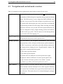
4.1 Navigation and control mode overview . . . . . . . . . . . . .
4.2 12 bit Voltage output DAC with serial interface . . . . . . . .
4.3 AMC brushless servo amplifier and EAD brushless dc motors
4.4 The different drive modes of Cool Robot . . . . . . . . . . . .
4.4.1 Waypoint following at full speed . . . . . . . . . . . .
4.4.2 Waypoint following at partial speed . . . . . . . . . .
4.4.3 Manual Operator . . . . . . . . . . . . . . . . . . . .
4.5 Perspective on further drive modes . . . . . . . . . . . . . . .
4.5.1 Charge cycle . . . . . . . . . . . . . . . . . . . . . .
4.5.2 Stationary data aquisition . . . . . . . . . . . . . . . .
4.5.3 High centered . . . . . . . . . . . . . . . . . . . . . .
.
.
.
.
.
.
.
.
.
.
.
.
.
.
.
.
.
.
.
.
.
.
51
52
53
55
57
59
61
62
64
64
65
66
4
.
.
.
.
.
.
.
.
.
.
.
.
.
.
.
.
.
.
.
.
.
.
.
.
.
.
.
.
.
.
.
.
.
.
.
.
.
.
.
.
.
.
.
.
.
.
.
.
.
.
.
.
.
.
.
.
.
.
.
.
.
.
.
.
.
.
CONTENTS
5
iv
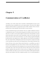
Communication of CoolRobot
5.1 IRIDIUM Communication . . . . . . . . . . . . . . .
5.1.1 The A3LA-I IRIDIUM modem . . . . . . . .
5.1.2 Prospect on further use . . . . . . . . . . . . .
5.2 Radio Communication . . . . . . . . . . . . . . . . .
5.2.1 The Kantronics KPC3plus packet radio modem
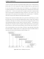
5.3 Controling the CoolRobot via radio link . . . . . . . .
5.3.1 Establish and terminate a connection . . . . . .
5.3.2 Manual drive mode . . . . . . . . . . . . . . .
5.3.3 Waypoint following . . . . . . . . . . . . . . .
5.3.4 Other commands and functions . . . . . . . .
.
.
.
.
.
.
.
.
.
.
.
.
.
.
.
.
.
.
.
.
.
.
.
.
.
.
.
.
.
.
.
.
.
.
.
.
.
.
.
.
.
.
.
.
.
.
.
.
.
.
.
.
.
.
.
.
.
.
.
.
.
.
.
.
.
.
.
.
.
.
.
.
.
.
.
.
.
.
.
.
.
.
.
.
.
.
.
.
.
.
.
.
.
.
.
.
.
.
.
.
.
.
.
.
.
.
.
.
.
.
.
.
.
.
.
.
.
.
.
.
67
68
70
81
81
83
92
93
95
97
98
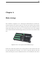
6
Data storage
102
6.1 Storage and retrieval of internal sensor data . . . . . . . . . . . . . . . . . . 103
6.2 The Campbell CR5000 and CR1000 dataloggers . . . . . . . . . . . . . . . . 108
7
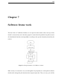
Software frame work
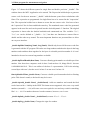
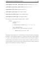
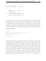
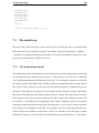
7.1 Definitions, libraries and variable declarations . . . . . . . . . . . . .
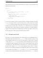
7.2 Start up sequence: initializing of variables, file system and serial ports
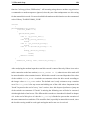
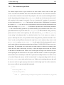
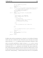
7.3 The main loop . . . . . . . . . . . . . . . . . . . . . . . . . . . . . .
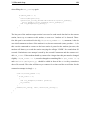
7.3.1 The modem input block . . . . . . . . . . . . . . . . . . . .
7.3.2 The main control block . . . . . . . . . . . . . . . . . . . . .
7.3.3 The modem output block . . . . . . . . . . . . . . . . . . . .
7.4 Different versions of the main programm . . . . . . . . . . . . . . . .
8
Results of the moving tests
8.1 GPS waypoint following position and navigation data
8.1.1 Autonomous waypoint following at full speed
8.2 Overall energy consumption on snow . . . . . . . . .
8.3 Rolling resistance . . . . . . . . . . . . . . . . . . .
8.4 Radio Interface and Communication . . . . . . . . .
.
.
.
.
.
.
.
.
.
.
.
.
.
.
.
.
.
.
.
.
.
.
.
.
.
.
.
.
.
.
.
.
.
.
.
.
.
.
.
.
.
.
.
.
.
.
.
.
.
.
.
.
.
.
.
.
.
.
.
.
.
.
.
.
.
.
.
.
.
.
.
.
.
.
.
.
.
.
.
.
.
.
.
.
.
.
.
.
115
116
119
124
124
125
127
130
.
.
.
.
.
135
135
136
143
144
145
A Functions and library overview
149
A.1 Overview of parameters and variables . . . . . . . . . . . . . . . . . . . . . 151
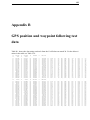
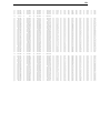
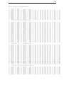
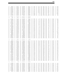
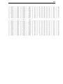
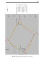
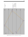
B GPS position and waypoint following test data
155
C Schematics overview
162
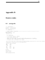
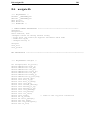
D Source codes
D.1 analogin.lib . . .
D.2 drive.lib . . . . .
D.3 gps.lib . . . . . .
D.4 navigate.lib . . .
D.5 radiocomm_e.lib
166
166
173
189
201
210
Bibliography
.
.
.
.
.
.
.
.
.
.
.
.
.
.
.
.
.
.
.
.
.
.
.
.
.
.
.
.
.
.
.
.
.
.
.
.
.
.
.
.
.
.
.
.
.
.
.
.
.
.
.
.
.
.
.
.
.
.
.
.
.
.
.
.
.
.
.
.
.
.
.
.
.
.
.
.
.
.
.
.
.
.
.
.
.
.
.
.
.
.
.
.
.
.
.
.
.
.
.
.
.
.
.
.
.
.
.
.
.
.
.
.
.
.
.
.
.
.
.
.
.
.
.
.
.
.
.
.
.
.
.
.
.
.
.
.
.
.
.
.
.
.
.
.
.
.
.
.
.
.
.
.
.
.
.
.
.
.
.
.
216
LIST OF FIGURES
v
List of Figures
1.1
Satellite Photo of Antarctica (Lever) . . . . . . . . . . . . . . . . . . . . . .
1
1.2
CoolRobot climbing sastrugi feature . . . . . . . . . . . . . . . . . . . . . .
2
1.3
Sastrugie features in Antarctica with 8 inch notebook for scaling . . . . . . .
6
2.1
Milled honeycomb getting bonded and put in place . . . . . . . . . . . . . .
8
2.2
Inserts with epoxy . . . . . . . . . . . . . . . . . . . . . . . . . . . . . . . .
9
2.3
Chassis without and with partition wall . . . . . . . . . . . . . . . . . . . . .
10
2.4
Top view of the support tube mounts and view along one of the axles . . . . .
10
2.5
The aluminum shaft collars . . . . . . . . . . . . . . . . . . . . . . . . . . .
11
2.6
First moving test of Cool Robot . . . . . . . . . . . . . . . . . . . . . . . .
12
3.1
Lat and lon on earth . . . . . . . . . . . . . . . . . . . . . . . . . . . . . . .
14
3.2
Visualization of most important terms for GPS navigation . . . . . . . . . . .
16
3.3
GPS positioning test on j parking lot at Dartmouth . . . . . . . . . . . . . . .
18
3.4
Options to initialize the GPS unit to output NMEA data . . . . . . . . . . . .
19
3.5
WinOncore for Motorola M12+ GPS receiver with GPS data in NMEA format
20
3.6
GPRMC example message . . . . . . . . . . . . . . . . . . . . . . . . . . .
21
3.7
Connector M12+ . . . . . . . . . . . . . . . . . . . . . . . . . . . . . . . .
22
3.8
Flowchart for basic navigation algorithm . . . . . . . . . . . . . . . . . . . .
23
3.9
Basingpoint and waypoint example ( drawing) . . . . . . . . . . . . . . . . .
25
3.10 Startup procedure 1 with Cool Robot pointing north . . . . . . . . . . . . . .
26
3.11 Startup procedure 1 with Cool Robot pointing south . . . . . . . . . . . . . .
27
3.12 Startup procedure 2 with Cool Robot pointing south . . . . . . . . . . . . . .
28
3.13 Example startup navigation (drawing) . . . . . . . . . . . . . . . . . . . . .
29
3.14 Basing point generating example (drawing) . . . . . . . . . . . . . . . . . .
30
3.15 Precision for decimal values . . . . . . . . . . . . . . . . . . . . . . . . . .
31
3.16 Spherical coordinates . . . . . . . . . . . . . . . . . . . . . . . . . . . . . .
31
LIST OF FIGURES
vi
3.17 Expression builder for "_double" . . . . . . . . . . . . . . . . . . . . . . . .
34
3.18 Sample SPI communication on serial port B . . . . . . . . . . . . . . . . . .
40
3.19 12-bit Control register sectioning . . . . . . . . . . . . . . . . . . . . . . . .
41
3.20 Straight binary vs. twos complement output format . . . . . . . . . . . . . .
42
3.21 Circuit to bias bipolar signals about Vref . . . . . . . . . . . . . . . . . . . .
43
3.22 ADC DIN and DOUT with analog input signal . . . . . . . . . . . . . . . .
43
3.23 Velocity monitor out vs. motor revolution . . . . . . . . . . . . . . . . . . .
47
3.24 High tilt angle interrupt handling sample . . . . . . . . . . . . . . . . . . . .
49
4.1
SPI Interface . . . . . . . . . . . . . . . . . . . . . . . . . . . . . . . . . .
54
4.2
DAC 16-bit data word . . . . . . . . . . . . . . . . . . . . . . . . . . . . . .
54
4.3
Voltage output vs. digital input . . . . . . . . . . . . . . . . . . . . . . . . .
55
4.4
Motor revolutions vs. input voltage . . . . . . . . . . . . . . . . . . . . . . .
56
4.5
Flowchart of drive mode waypoint following at full speed . . . . . . . . . . .
59
4.6
Screen shot of dynamic C code for waypoint following at full speed . . . . .
60
4.7
Overview of motor placement . . . . . . . . . . . . . . . . . . . . . . . . .
63
4.8
Drive mode charge cycle . . . . . . . . . . . . . . . . . . . . . . . . . . . .
64
4.9
Drive mode stationary get data . . . . . . . . . . . . . . . . . . . . . . . . .
65
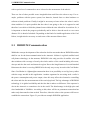
5.1
Example for an IRIDIUM modem application . . . . . . . . . . . . . . . . .
69
5.2
FDMA versus TDMA . . . . . . . . . . . . . . . . . . . . . . . . . . . . . .
70
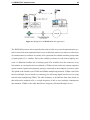
5.3
Motorola 9505 A3LA-I IRIDIUM modem . . . . . . . . . . . . . . . . . . .
71
5.4
SAF2040-E mobile flat mount antenna . . . . . . . . . . . . . . . . . . . . .
71
5.5
Some sample commands with explanation (AT manual for A3LA) . . . . . .
73
5.6
Example for different ways to type commands (AT manual for A3LA) . . . .
73
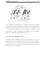
5.7
Components needed for packet radio communication . . . . . . . . . . . . .
82
5.8
KPC3plus front view . . . . . . . . . . . . . . . . . . . . . . . . . . . . . .
83
5.9
1300/2100Hz Frequency Shift Keying . . . . . . . . . . . . . . . . . . . . .
84
5.10 Basic wiring of the KPC3plus radio modem . . . . . . . . . . . . . . . . . .
85
5.11 Pinouts MAX3232 RS232 line driver/receiver . . . . . . . . . . . . . . . . .
86
5.12 Wiring of the MAX3232 on the RCM3100 evaluation board . . . . . . . . .
87
5.13 Wiring suggestion for ICOM radios . . . . . . . . . . . . . . . . . . . . . .
87
5.14 AUTOBAUD routine running on Hyperterminal . . . . . . . . . . . . . . . .
88
5.15 MYCALL command using Hyperterminal . . . . . . . . . . . . . . . . . . .
89
5.16 ECHO ON/OFF command using Hyperterminal . . . . . . . . . . . . . . . .
90
LIST OF FIGURES
vii
5.17 Unsuccessful and successful attempt to connect. . . . . . . . . . . . . . . . .
90
5.18 Structure of KPC3plus data packets . . . . . . . . . . . . . . . . . . . . . .
91
5.19 Screen shot of Hyperterminal while in manual drive mode . . . . . . . . . .
96
5.20 Screen shot of Hyperterminal: sending waypoints . . . . . . . . . . . . . . .
99
5.21 Screen shot of Hyperterminal: requesting CoolRobots status . . . . . . . . . 100
5.22 Screen shot of Hyperterminal: requesting data from CoolRobot
. . . . . . . 101
6.1
Picture of the Campbell Scientific CR1000 datalogger . . . . . . . . . . . . . 102
6.2
Picture of Z-Worlds RCM3100 core module . . . . . . . . . . . . . . . . . . 103
6.3
Screen shot of FS2 sample program showing specifications of the Flash memory105
6.4
Screen shot of "Short Cut" first step: edit measurement interval . . . . . . . . 109
6.5
Screen shot of "Short Cut" second step: choosing sensors . . . . . . . . . . . 110
6.6
Screen shot of "Short Cut" third step: select tables . . . . . . . . . . . . . . . 111
7.1
Rough schematic of CoolRobots software . . . . . . . . . . . . . . . . . . . 115
7.2
Flow chart of "mainprogV0.34" . . . . . . . . . . . . . . . . . . . . . . . . 131
7.3
Flow chart of "mainprogV0.35" . . . . . . . . . . . . . . . . . . . . . . . . 133
8.1
Cool Robot navigating to a waypoint on lake mascoma . . . . . . . . . . . . 136
8.2
Navigation routine at startup . . . . . . . . . . . . . . . . . . . . . . . . . . 139
8.3
Waypoint and basing point shifting sample . . . . . . . . . . . . . . . . . . . 140
8.4
Off bearing with basing points every 100 m . . . . . . . . . . . . . . . . . . 141
8.5
Off bearing with basing points every 500 m . . . . . . . . . . . . . . . . . . 141
8.6
Current draw data on snow . . . . . . . . . . . . . . . . . . . . . . . . . . . 143
8.7
Screen shot of "mapquest.com" showing the starting point and the point the
last transmission was received before losing connection . . . . . . . . . . . . 147
B.1 Waypoint following with basing points every 100 m . . . . . . . . . . . . . . 160
B.2 Waypoint following test with basingpoints on waypoints . . . . . . . . . . . 161
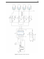
C.1 2nd order Butterworth Filter for the 2 axis tilt sensor . . . . . . . . . . . . . 163
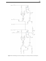
C.2 Conditioning circuit for the analog motor velocitiy and motor current inputs . 164
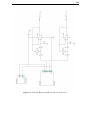
C.3 Schematic of DAC connections . . . . . . . . . . . . . . . . . . . . . . . . . 165
LIST OF TABLES
viii
List of Tables
1.1
Main topics of work on Cool Robot. . . . . . . . . . . . . . . . . . . . . . .
3
3.1
NMEA-0183 Specification Revision 2.0.1. . . . . . . . . . . . . . . . . . . .
20
3.2
GPRMC message. . . . . . . . . . . . . . . . . . . . . . . . . . . . . . . . .
21
3.3
Sample structure GPSPosition current_pos. . . . . . . . . . . . . . . . . . .
24
3.4
Sample using structure _double. . . . . . . . . . . . . . . . . . . . . . . . .
36
3.5
Analog input channels. . . . . . . . . . . . . . . . . . . . . . . . . . . . . .
37
3.6
ADC / DAC ribbon cable. . . . . . . . . . . . . . . . . . . . . . . . . . . . .
38
3.7
EVAL-AD7490CB power supplies. . . . . . . . . . . . . . . . . . . . . . . .
39
3.8
Switch and link options on EVAL-AD7490CB. . . . . . . . . . . . . . . . .
39
3.9
Sensor range handling functions. . . . . . . . . . . . . . . . . . . . . . . . .
49
4.1
Serial port connections and functions for RCM. . . . . . . . . . . . . . . . .
51
4.2
Control and drive mode overview . . . . . . . . . . . . . . . . . . . . . . . .
53
5.1
Modifiers for Dn. . . . . . . . . . . . . . . . . . . . . . . . . . . . . . . . .
75
5.2
Modifiers for En. . . . . . . . . . . . . . . . . . . . . . . . . . . . . . . . .
75
5.3
Modifiers for Zn. . . . . . . . . . . . . . . . . . . . . . . . . . . . . . . . .
76
5.4
Modifiers for &Cn. . . . . . . . . . . . . . . . . . . . . . . . . . . . . . . .
76
5.5
Modifiers for &Dn. . . . . . . . . . . . . . . . . . . . . . . . . . . . . . . .
77
5.6
Modifiers for &Kn. . . . . . . . . . . . . . . . . . . . . . . . . . . . . . . .
77
5.7
Modifiers for &Wn. . . . . . . . . . . . . . . . . . . . . . . . . . . . . . . .
77
5.8
Possible values for +CBST command. . . . . . . . . . . . . . . . . . . . . .
78
5.9
Example: originating a data call. . . . . . . . . . . . . . . . . . . . . . . . .
79
5.10 Example: incoming data call. . . . . . . . . . . . . . . . . . . . . . . . . . .
79
5.11 Overview of AT command result codes. . . . . . . . . . . . . . . . . . . . .
80
5.12 Pinouts RS232. . . . . . . . . . . . . . . . . . . . . . . . . . . . . . . . . .
85
5.13 Control keys for manual driving. . . . . . . . . . . . . . . . . . . . . . . . .
95
LIST OF TABLES
ix
5.14 Components of navigation data string. . . . . . . . . . . . . . . . . . . . . .
97
5.15 Overview of commands to enter/switch drive modes. . . . . . . . . . . . . .
99
6.1
Possible values for the ResultCode. . . . . . . . . . . . . . . . . . . . . . . . 112
6.2
Possible values for BufferControl. . . . . . . . . . . . . . . . . . . . . . . . 113
6.3
Possible values for DataFormat. . . . . . . . . . . . . . . . . . . . . . . . . 114
7.1
Overview of status variables. . . . . . . . . . . . . . . . . . . . . . . . . . . 121
8.1
Parameters for waypoint following at full speed 22 mar. . . . . . . . . . . . . 137
8.2
Distances and bearings for the waypoints "lake mascoma bridge". . . . . . . 138
8.3
Parameters for waypoint following at full speed 24 mar. . . . . . . . . . . . . 140
8.4
Overview of distances. . . . . . . . . . . . . . . . . . . . . . . . . . . . . . 142
LIST OF SYMBOLS
x
List of symbols and abbreviations
ADC
Analog to Digital Converter
Baud
One signalling element per second.
bp
basing point
char
8 bit character
cp[1]
current point for navigation use
cp[2]
last current point used for current bearing
CR
Carriage Return also ’\r’
CS
Chip Select - is used to start a conversion on the selected channel
CTS
Clear To Send. A flow control signal in serial interfaces.
DCD
Data Carrier Detect. This signal indicates a connection
to the far-end modem for data transfer.
DAC
Digital to Analog Converter
DIN
Digital Input for a serial port
DOUT
Digital Output line for a serial port
DSR
Data Set Ready. Another flow control signal.
DTE
Data Terminal Equipment e.g. a personal computer running terminal software.
DTR
Data Terminal Ready. Yet another flow control signal.
float
32 bit IEEE-floating point
GPRMC
Recommended Minimum Specific GPS-data
GPSPosition
structure implemented in the code for latitude and longitude
of a position
GSM
Global System for Mobile communications.
ICD-GPS-200
Interface Control Document defining characteristics of
and data for the GPS L1 and L2 Signals in Space (SIS)
LIST OF SYMBOLS
int
16 bit signed integer value
I/O
Input and Output
IRLP
Iridium Radio Link Protocol
ISU
Individual Subscriber Unit (IRIDIUM modem)
lat
latitude
LF
Line Feed, same as new line ’\n’
lon
longitude
NMEA
National Marine Electronics Association
NMEA 0183
Interface Standard that defines specific sentence formats for
xi
a 4800-baud serial data bus
PTT
Push To Talk
RI
(V.24 Signal) Ring Indicate. ISU signal that indicates an incoming call.
RS232
Today named EIA232 and is a common interface standard for data communication
RTS
Request To Send.
RX
Receive signal
SCLK
Serial Clock - Internal Clock of Jackrabbit
SG
Signal Ground
SPI
Serial Peripheral Interface (three wire)
TTFF
Time To First Fix
TX
Transmit signal
wp
waypoint
XON/XOFF
A standard flow control method.
1
Chapter 1
Introduction
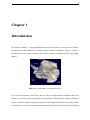
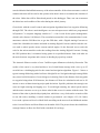
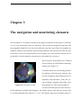
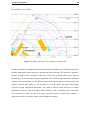
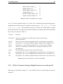
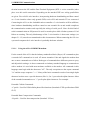
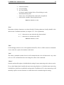
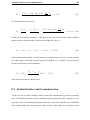
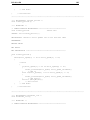
The Antarctic Plateau - a large, high altitude mass of ice and snow, covering most of Antarctica and impacts the atmospheric circulation of the Southern Hemisphere. Figure 1.1 shows a
satellite photo of the entire continent. The Antarctic Plateau is composed of the region highlighted.
Figure 1.1: Satellite Photo of Antarctica (Lever)
It is of course extremely cold and dry, but it is also very high and the atmosphere above the
plateau is very calm with low wind speeds at all latitudes. That makes the Antarctic Plateau a
unique location to study the upper atmosphere at high magnetic latitudes, providing a stable
environment for sensitive instruments that measure the interaction between the solar wind and
2
the Earth’s magnetosphere, ionosphere, and thermosphere [1].
Few Robots have been build to discover the Antarctic Plateau. They were very heavy and
driven by combustion engines. These expeditions need either a high assignment of personnel, which is a problem in the harsh weather conditions in Antarctica, or a large transportation
capacity which is very expensive, limited by the small size of the Twin Otter arid transport aircraft flying within Antarctica and entail hazards at remote landing and takeoff sites. Carnegie
Mellon University for example developed NOMAD, a 725 kg gasoline-powered robot for
polar and desert environments with a size of 2.4x2.4x2.4m [2]. The much smaller Spirit and
Opportunity are Mars Exploration Rovers from NASA/JPL. Each 2.3x 1.6x 1.5m rover weighs
174 kg and has a top speed of 5 cm/s [3] and is powered by a multi-panel solar array.
The task was to build an Autonomous Mobile Robot which can be released at the South Pole
station and traverse on the Antarctic Plateau during the austral summer within a range of 500
km in a time of 2 weeks without any maintenance. That is possible, because the robot is powered by renewable energy, the sun. The Antarctic Plateau gives very good reasons for using
solar energy. During the austral summer month the direct insolation from the sun averages
1000 W/m2 . Also the reflected sunlight by the large flat snow areas is significant. The robot
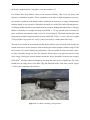
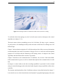
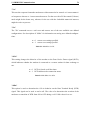
should have an empty mass of less than 75kg and should fit in the Twin Otter aircraft. Figure
1.2 shows the completed robot chassis.
Figure 1.2: CoolRobot climbing sastrugi feature
3
The basis for our work was the Diploma Thesis from Guido Gravenkötter and Gunnar Hamann
[4] and the honor‘s thesis of Alex Price [5]. Reference [5] deals with the conceptional work
on the robot and the major influence on the design of a solar powered robot. Hamann‘s and
Gravenkoetter‘s contribution was to prove the viability of the project. They tested different
components such as the brushless dc-motors, the li-ion batteries and the power supply in a
cold chamber to see the influence of cold temperatures down to -40◦ C.The conclusion was
that the new generation of solar panels will provide enough energy needed for the propulsion.The other conclusion of [4] was that the navigation has to be based on waypoints and
GPS data only, because a magnetic compass does not work on the high magnetic latitudes on
the Antarctic Plateau.
Reference [5] completed the robot design, including CAD models of all components and
structural analysis. The mechanical design of the robot is based on a very light but strong
honeycomb composite made of fiberglas and Nomex.
This thesis describes three different parts of work on the Cool Robot:
1.
2.
3.
assembling of the chassis
navigation and control
communication and datalogging
Table 1.1: Main topics of work on Cool Robot.
The first part is the assembling of the honeycomb chassis and the motors and drive trains.
CoolRobot project started in winter 2003/2004 with the conceptional work. During the summer 2004 Alex Streeter, Alex Price and Dan Denton made most of the mechanical parts for
the robot. The honeycomb panels were cut in pieces for the main chassis, the solar panel attachment arms the stiffeners, and the lid. The EAD-brushless motors were mounted to the
gearhead and ready for their implementation in the chassis. The aluminum rims for the 16
inch or the 20 inch ATV tires were welded to the axis. On the logic side, the jackrabbit itself
was ready for testing, because it was mounted to the evaluation board. The circuit for the 8
channel Analog Digital Converter MAX186 for reading the analog sensors and the Digital
Analog Converter MAX536 to control the motors was build. The design of the solar power
4
system is the work of Alex Streeter’s M.S. Thesis. Five separate, custom-built solar panels
feed power onto a common bus, which is then distributed to the motors and housekeeping
electronics. A bank of Li-Ion batteries act as a buffer for the bus and provide auxiliary power.
The first part of our work was to assemble the chassis, adapt the motors to the chassis, and
provide the support tubes for the axis. Configurating the microcontroller to communicate with
the ADC the DAC, the GPS unit, the Datalogger and the modem would be the main part of
our work. Finally, we had to program the different algorithms to drive the motors, read the
different sensors, communicate with the modems, read the gps-data, and control the robot in
various modes of operation.
Toni‘s main tasks are the communication between the robot and a human operator and the
storage and retrieval of data the robot collects during it’s journey. The only way to stay in
touch with the robot while it is traveling around on the Antarctic Plateau is a connection over
IRIDIUM-modem, which is at the moment the only provider of truly global mobile satellite
voice and data solutions. The system provides a complete coverage of the earth‘s oceans, airways and most important for our application, the polar regions. With this connection the robot
is able to report problems, transmit a portion of the collected data, or request new waypoints.
On the other hand, an operator has the possibility to check the condition of the robot, request
data and send new or changed waypoints. When the robot is deployed in the Antarctic it will
equipped with an IRIDIUM transceiver. The big disadvantage of this system is the high price
for this unlimited availability. The transceiver itself is priced around $1200 and every minute
of connection costs $2 within the United States and $7 elsewhere in the world. Therefore another, cheaper system will be used during the development of the robot and the first field tests
in Greenland. The easiest way to establish a wireless connection and transmit digital data is
a radio connection using a data modem. With the help of two handheld radios and two radio
modems one is able to control the motion of the CoolRobot manually or monitor the behaviour
of the machine while navigating autonomously over a distance of approximately 2 km.
The CoolRobot will also be equipped with a datalogger to record scientific data from the
payload. This data is analog and can be retrieved when the robot returns to its base. Especially
during testing and the first run in the Antarctic all the sensor data the robot uses is a matter of
particular interest. So, all this digital data will be stored too. The latest sensor-readings will be
5
stored within the limited flash memory of the microcontroller. If the robot encounters a critical
situation this data will be send to the operator who then is able to reconstruct the situation of
the robot. Older data will be filtered and passed to the datalogger. Thus, one can reconstruct
the behaviour and condition of the robot during the whole journey.
Goetz deals with the overall control and navigation algorithm based on waypoint following
through GPS. The robot‘s main intelligence are two microprocessors which are programmed
in Dynamic C a computer language similar to C++. One is used for the power management,
which is Alex Streeter’s M.S.thesis. The second microcontroller is for communication. It communicates with the GPS-Receiver to get the GPS-data, with a Digital-Analog-Converter to
control the 4 brushless dc-motors and with an Analog-Digital-Converter which reads the sensors such as wheel speeds, motor currents and tilt angles. So the first task was to write the
code for the microcontroller to take the readings from the Analog-Digital-Converter. Getting
the GPS position data, it calculates basing points in a specified distance from each other on
the track between waypoints and corrects its heading by open loop control.
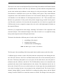
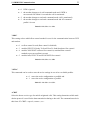
The Antarctic Plateau consists of over 5 million square kilometers relatively flat terrain. The
surface of the snow is very hard and has a lot of wind blown sastrugi with a size up to 25
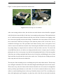
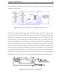
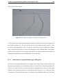
cm which are a challenging task for the control and navigation algorithm. Figure 1.3 shows a
typical sastrugi field along with a breifcase of height 20 cm. Navigation through sastrugi fields
may cause brief dislocation of several degrees in bearing. But for the distance from waypoint
to waypoint being about 50 kilometers, the distance off from its calculated track can be 20
meters or more without incurring major path deviations. Specific problems the sastrugis can
cause are high centering and tipping over. To avoid high centering, the wheel speed sensors
and the motor currents are set up to detect wheels that are not in contact with the snow. The
bottom of the robot is plated with polyethylene, which has a very slick surface to make a slide
to one side easier, enabling a control routine to get unstuck. (see chapter 4.5.3) Dr. James
Lever took a picture on Ross Ice Shelf while travelling on the traverse from McMurdo station
to the Leverett Glacier and Polar Plateau in december 2004. The picture shows the wind blown
sastrugi features on Ross Ice Shelf with a notebook 20 cm large.
6
Figure 1.3: Sastrugie features in Antarctica with 8 inch notebook for scaling
To avoid the robot from tipping over, the 3-axis-tilt-sensor sends an interrupt to the control
algorithm (see chapter 3.3.6).
This thesis starts with the assembling process for Cool Robot. We hope to give a summary
of good practices for handling the honeycomb and some useful hints for refining next Cool
Robot design.
Chapter 3 deals with the navigation of Cool Robot and provides all the necessary information
to understand the basic mode of operation of the gps receiver as well as the main navigation
program of Cool Robot and the monitoring of the analog sensors. In chapter 4 the control
algorithms and the different drive modes are presented.
Chapter 5 introduces to the communication of CoolRobot. An overview of the future IRIDIUM communication is given, as well as a detailed description of the communication via radio
link.
In chapter 6 a short outline on the data recording capabilities is presented. On the on hand
using an external datalogger and on the other hand using the storage capabilities of the micro
controller.
The structure and functionality of the CoolRobots software is described in detail in chapter 7.
It can also be seen as a basic introduction to the DynamicC programming language with some
7
of its advantages and disadvantages for our application.
The test results such as current draw and energy consumption, waypoint following position
data, and communcation protocol are presented in chapter 8
8
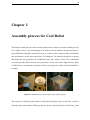
Chapter 2
Assembly process for Cool Robot
This chapter should give the reader an impression of how extensive even the assembly process
for a simple robot is. By documenting weak points in the mechanical design and minor or
major difficulties during the mechanical work, we want to achieve improvements in reliability
and performance for the next generation of CoolRobots. The outcome should be an update
that makes the next generation of CoolRobots better and a choice to beat! The combination
of the honeycomb chassis and the new generation of solar cells with a high efficency helps
CoolRobot to be an alternative solution for heavy and expensive robots such as NOMAD for
example.
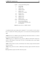
Figure 2.1: Milled honeycomb getting bonded and put in place
The structure of the honeycomb allows to mill just the fiberglass layer on one side, to fold or
bend the panel perpendicular. When got into the project, almost all parts for the honey comb
9
chassis where already cut and milled by Alex Streeter and Alex Price. Some of the aluminum
parts for the drive train where also available, like the wheels, axles and the retainers for the
motors and gear heads. Thus, our task was finishing the remaining parts, and putting them
together to a rolling chassis.
The first step was the gluing of the chassis body.
Before actually gluing it together we had to drill
holes for the support tubes and the inserts for
mounting the motors and the top lid, since it is
easier much easier to do this as while the body
still is a flat piece of honey comb, instead of an
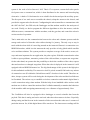
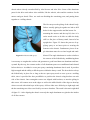
upright box. Figure 2.2 shows the process of applying epoxy to an insert prior to securing the
fastener to the chassis. Furthermore pieces of angle aluminum must be cut into length and sandFigure 2.2: Inserts with epoxy
blasted. The angle aluminum is used to reinforce
the corners of the folded body, sandblasting them
is necessary to roughen the surface and guarantee a good bond between aluminum and honeycomb. By the way, the contact surface of all aluminum parts were sandblasted and cleaned
before their use. As adhesive a two part epoxy containing aluminum dust is used. It provides
high strength and the ability to fill the spaces within the honey comb. The best choice to keep
the folded body in place for as long as the two part epoxy needs to cure up was a welding
table, since it provided the best possibilities to position the chassis using brackets on each
side of the chassis. One rectangular corner was aligned with brackets, to start the gluing in
this corner. All contact areas at the edges as well as the milled inside of the edges to bend up
where covered with a thin layer of the epoxy. All four sides were folded up to right angle and
the the remaining two sides were fixed by two more brackets. The result is shown in right half
of figure 2.1. After aligning the chassis correctly the angle aluminum was glued to the insides
of all four corners.
10
Figure 2.3: Chassis without and with partition wall
The next step was adding two partition walls to the corners of the chassis where the motors
are located. Since the motors are screwed to the chassis box itself and the partition walls we
also drilled the holes for this connection before gluing the walls to the box. That was not
an ideal solution, since there is no guarantee for a correct alignment of the motors. Thus, on
further generations of CoolRobots the holes in the partition walls and the chassis box should
be drilled after adding the mounts for the axle to align the motors as exact as possible and
avoid unnecessary high friction within the drive train. To add more strength to the partition
walls angle anluminum was used to reinforce the connection on either side of the walls and
on the bottom.
Figure 2.4: Top view of the support tube mounts and view along one of the axles
11
After that the mounts for the support tubes (see figure 2.4) were glued to the chassis. To assure
an exact alignment of both support tubes on one axle a long piece of the aluminum tube used
for the support tubes was used through the tube holes on both sides of the robot. The tube
remained within the axle over night until the epoxy cured up completely. Since the mounts on
the outside consist of two independent rings some of the epoxy could have reached the tube,
thus to avoid gluing the tube to the mounts we moved it from time to time.
In the meantime the shaft collars were milled and
the inner parts of the rims were welded to the actual axles. Furthermore, all inserts were glued to
the chassis, and the motor and gear heads were
mounted too. For gluing the inserts we coated the
contact areas with epoxy, put both parts with a
Figure 2.5: The aluminum shaft
collars
screw and nut to the desired hole and tightened
the screw carefully until both parts of the inserts
engaged.
The next step was finishing the support tubes and gluing them in place. The tubes were cut to
length and on one side the inner diameter of the tube was enlarged a little bit to the bearings
within. Furthermore a groove for the retaining ring was milled to the very end of the tube.
The finished support tube was now glued to the mounts also using the two part epoxy. After
this step the whole drive train was mounted to the chassis, beginning with screwing the shaft
collars to the gear head, then fitting the bearings to the support tubes and fastening them
with the retaining rings. Now, the axles could be inserted and screwed to the shaft collars
and finally the wheels were screwed to the axles. As the rolling chassis was finished the
electronic components were added to the chassis. The motor controllers were mounted to the
side walls of the chassis near their appropriate motor using two screws for each controller
glued to the walls. By the time we finished the assembly to a drive able robot, the first test
pieces of software were finished too. One of them was a routine to adjust the output of the
motor controllers via the DynamicC compiler window and keyboard inputs. So we started first
driving tests. At the very beginning we droe just within the building but we soon decided to
take it outside to check its maneuverablity, speed and also the strength and flex of the chassis.
12
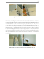
Figure 2.6 shows photos from the first outdoor tests.
Figure 2.6: First moving test of Cool Robot
After some testing with the robot, the decision was made that the robot should be equipped
with 20 inch tires instead of the 16 inch tires it was running at the moment. The benefits herein
are a 2 inch increased ground clearance and due to the fact the 20 inch tires are slightly wider
also a decreased ground pressure and sinkage. Furthermore the tread pattern of the 20 inch
tires seemed more efficient for driving on snow than the pattern of the 16 inch tires. So we
switched to the larger tires. This procedure took almost one day, since it was quite a bit of
work to remove the small tires from the rims. Removing the first half of the rims was pretty
easy using clamps to compress the tire until one of the two halves was free. To remove the
second half from the tire, we had to use clamps and wood to move it step by step. In contrast,
putting the new tires on was pretty easy and involved putting both halves of the rims together
with some new sealing compound and the new tires in between and inflating the tire to about
30psi until the tire pops into the correct place on the rim. To help the tires sliding on the rim
some soap and water was used as lubricant.
The last part of the Assembly process was fitting the top lid to the robots chassis. The first step
was cutting the sidewalls of the lid to their final height and drilling the holes for the inserts.
This was not easy, since the inserts on the chassis sidewalls were not exactly in a straight line
and in perfectly equal distances to each other. So we had to custom fit almost every hole to
achieve as much matching inserts on the top lid and the chassis itself. The exact fitting was
done while gluing the top lid together: we glued one side of the lid at a time and focused the
13
inserts of the top lid by screwing them to their respective insert on the chassis. Doing one
side after the other in this manner we assured the best possible fitting. The next day when
the epoxy on all inserts was cured completely we started with the actual cluing of the top lid.
We screwed one side of the lid to the chassis and then coated all necessary contact areas with
epoxy. After this the lid was folded down to the chassis and the other three sides were focused
too. Since almost all insert holes were focused with screws the lid cured up keeping exactly
the right shape. Finally a hole was drilled to the middle of the top lid trough which cables for
the GPS antenna, the radio and the Jackrabbits programming cable can be lead.
During all the testing the Cool Robot’s concept proved itself by being an easy and reliable
robot. The only real problem we encountered during this time was the connection between
gear head and axle. The aluminum shaft collars produced some problems with the drive train.
The aluminum does not provide enough strength in this application, there is too much slackness at the key on the gear heads axle. Thus the wheels can turn several degrees without any
movement of the motors. Furthermore the aluminum of the shaft collars and the robots axle
bond together due to some small parts of aluminum in between. This made big problems when
trying to disassemble the drive train. Therefore the suggestion is to use another material, e.g.
steel, for the shaft collars in the future. Maybe not only on further generations of Cool Robot
but also before testing in Greenland and definitely before deploying it in the Antarctic.
14
Chapter 3
The navigation and monitoring elements
The navigation of Cool Robot is limited by the budget restrictions for the project. Cool Robot
is a low cost autonomous robot for Antarctica. The fact that the magnetic South Pole and
the geographic South Pole vary from each other does not have great effect on navigation by
magnetic compass in our latitudes, but the bearing difference does increase the closer one gets
to the Poles. Precise bearing information for navigation use on the Antarctic Plateau can be
provided by a triaxial magnetic compass but is not intended for our project.
Due to expense, the navigation for Cool Robot
is based entirely on GPS(Global Positioning
System) (see chapter 3.1).
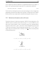
Coordinate planes for determining positions
on earth have existed for many centuries. History has brought up many different ways of
longimetry and goniometry. Today the system of latitude, longitude and height is the
Figure 3.1: Lat and lon on earth
most popular one. The prime meridian in
Greenwich and the equator are the references
for the definition of latitude and longitude. The latitude degrees start from the equator with
0◦ to North and South Pole with 90◦ ‘N‘ or ‘S‘. The distance between two latitude degrees is
15
always the same and does not change. For one latitude degree being divided into 60 arc minutes which have a distance of 1 nautic mile, the distance between two degrees is 111.136 km.
One latitude minute is again divided into 60 seconds. Longitude degrees and minutes are also
divided into 60 arc minutes and these again in 60 arc seconds. The longitude is measured up
to 180◦ west or east. The distance between two longitude degrees is not constant and changes
with latitude.
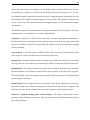
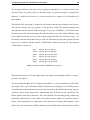
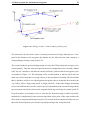
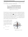
The following chapter deals with the main navigation algorithm of the Cool Robot. The most
important terms are explained here for better understanding:
waypoint: A waypoint is a GPS position consisting of latitude and longitude transmitted to
the robot by the user. A maximum of 100 waypoints can be saved in an array. By means of the
waypoint coordinates and the current position, the distance to the waypoint and the heading
can be calculated.
current point: A GPS data string in NMEA format from which the current position of the
robot is parsed. Used to calculate and correct the traveled course.
basing point: A GPS position generated in a distance given by the user on the track connecting
two waypoints. In our case they are generated every 1000 m to reduce the offset from the track.
initial distance: The distance between two waypoints. For the first navigation cycle at startup,
the initial distance is the distance from the first current position to the first active waypoint.
The initial distance does not change during navigation until the waypoint is reached and the
next waypoint is activated.
initail bearing: The bearing between two waypoints. For the first navigation cycle at startup,
the initial bearing is the bearing from the first current position to the first active waypoint. The
initial bearing does also not change and is calculated together with the initial distance.
distance to waypoint/ basing point/ current distance: The distance between the current
position and the mentioned point in km. The current distance is the distance between the last
two current positions.
16
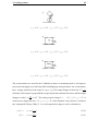
bearing to waypoint/ basing point/ current bearing/ off bearing: The bearing on which
one would reach the waypoint/ basing point when traveling on. The bearing is measured in
true degrees from north, counted clockwise. The current bearing is calculated between the last
two current positions. The off bearing is the number of degrees the robot needs to turn to head
to the desired position (e.g. waypoint).
offset from track: The offset from track is the smallest distance to a direct connection between two waypoints. The length of the perpendicular to the track through the current position.
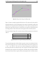
Figure 3.2: Visualization of most important terms for GPS navigation
The main principle of the navigation is waypoint following (see chapter3.2). Cool Robot receives GPS data, which includes latitude and longitude for the current position. The user
provides a list of waypoints he wants the robot to reach. By calculating its current position the
robot then travels on a predetermined path to the next waypoint. When within a certain range
of that waypoint, the path to the next waypoint will be calculated. For two waypoints being
away from each other over 10 km, the robot generates basing points (see chapter 3.2) on the
track in a distance of 1 km to each other.
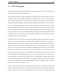
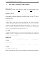
3.1 GPS Navigation
3.1
17
GPS Navigation
Everybody has heard about Global Positioning System, but how exactly can a robot travel in
Antarctica only relying on the GPS Signal?
The NAVigation Satellite Timing and Ranging (NAVSTAR) Global Positioning System is an
all weather, radio based, satellite navigation system that enables users to accurately determine 3- dimensional position, velocity and time worldwide. The GPS-System was originally
invented for the military and is run by the American Department of Defense. The System consists of 24 satellites operating in 12-hour orbits in an altitude of 20,200 km around the Earth
that emit signals which can be received on Earth by GPS receivers. The constellation is divided
in six orbital planes, each with 4 satellites equally spaced around the equator and inclined at
55 degrees. The GPS receiver on earth determines position by passive multi-lateration. With
knowledge of the transmission time for each signal, the distance to each satellite with known
coordinates in space can be calculated.
To determine the correct 3 dimensional position (latitude, longitude and altitude) the receiver
needs the clock offset. Therefore, a minimum of four satellite observations are required to
mathematically solve for the four unknown receiver parameters. If the altitude is known, then
only three satellite observations are required. However, that is not a guarantee for consistent
accuracy. The accuracy depends on the number of satellites tracked. With 5 or more satellites
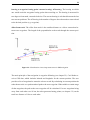
the receiver‘s position can be accurate up to a few meter (Figure 3.3). The accuracy can be
increased up to less than 1 meter with Differential GPS (DGPS). Hereby the receiver‘s signal
is corrected with a second GPS signal send out by a stationary GPS receiver on Earth. The
correction signal is sent in a longwave signal. The correction stations are generally provided
in coastal regions and driven by the coast guard. CoolRobot will have a DGPS receiver for the
testing in Greenland but for the navigation during this thesis it is equipped with a Motorola
Oncore M12+ receiver (see chapter 3.1.1).
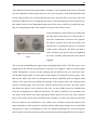
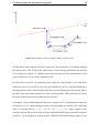
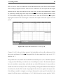
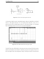
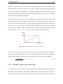
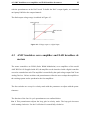
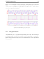
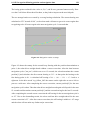
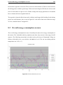
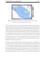
Figure 3.3 shows some driven tracks against the background of the j parking lot on Dartmouth
campus. The speed was around 1 mph. The gps position data was evaluated and charted with
excel. It should be used to receive an impression on the GPS‘s accuracy. During the testing,
3.1 GPS Navigation
18
five satellites were tracked.
Figure 3.3: GPS positioning test on j parking lot at Dartmouth
Besides the latitude and longitude position information the NMEA-0183 GPS data string also
includes information about speed over ground and current bearing. The speed over ground is
accurate enough to tell a movement of the robot, even at low speeds around 0.5 m/s, whereas
the bearing is of no use for the navigation algorithm. The GPS bearing is internally calculated
with the two last positions. As the distance between two points apart 1 second in time, the
distance between these points is 1 m, assumed 90 % of the robot‘s top speed. That makes
a precise bearing calculation impossible. The result is, that the robot will have no usable
information about the current heading, while making a turn or standing still on one point.
The conclusion is to have an open loop course correction based on course GPS readings, or
upgrade the robot if necessary with a triaxial magnetic compass.
3.1 GPS Navigation
3.1.1
19
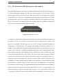
The Motorola Oncore M12+ GPS receiver
The GPS receiver on the evaluation board M12+ is provided with +10 V supply voltage.
The I/O-command format is Motorola Binary at 9600 baud. The commands can be used to
initialize, configure and control the receiver. The receiver does also provide I/O-commands
in NMEA-0183 format at 4800 baud, but these commands can only be used to change the
transmitted GPS data string (e.g. output rate). For all I/O-commands see M12+ receiver user‘s
guide chapter 5. The best way to initialize the receiver is by using the software WinOncore on
a PC. The serial port has to be connected to the GPS receiver with the provided 9-pin serial
cable. The serial port on the PC has to be opened at 9600 baud.
If the receiver is started up after a longer non-operated period of time, the user should allow
the receiver 3 to 5 minutes to power up. That time is called TTFF (Time To First Fix). The
receiver must now perform a Cold Start, where position, time, and almanac information are not
available. The satellite almanac files each contain information about GPS reference week, the
almanac reference time, required data to identify a satellite, satellite health status, longitude
of orbital plane and more (see ICD-GPS-200 for detailed description). Note that a cold start
is not a serious problem, but TTFF will be somewhat longer than if the information had been
available. The main thing to keep in mind is that the receiver coming up in a Cold Start
scenario is defaulted to Motorola Binary protocol, and NO MESSAGES are ACTIVE. The
receiver is running through its normal housekeeping routines, developing new fix data, etc.,
but it will not send any of this data out of the serial port until it is requested.
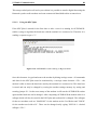
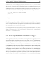
Figure 3.4: Options to initialize the GPS unit to output NMEA data
3.1 GPS Navigation
20
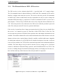
Using the software Winoncore, the receiver can be initialized easily by selecting the desired
output format and rate from once a second to once every 9999 seconds. After setting the output
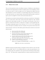
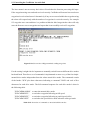
format, NMEA Protocol has to be enabled (Figure 3.4).
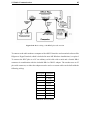
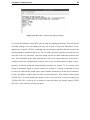
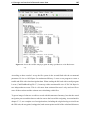
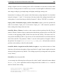
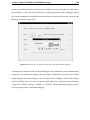
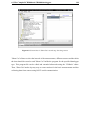
The GPS data string sent to the serial port is displayed in the command monitor window
(Figure 3.5) and accessed by "Cmd Mon". The receiver now is ready to be connected with
serial port C on the Jackrabbit microcontroller (Figure 3.7).
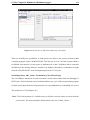
Figure 3.5: WinOncore for Motorola M12+ GPS receiver with GPS data in NMEA format
The software compiles the Motorola Binary I/O-commands to initialize or configure the GPS
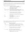
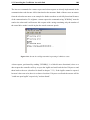
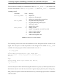
receiver. Once in NMEA format the user can decide between following different NMEA output messages:
Message
GPGGA
GPGLL
GPGSA
GPGSV
GPRMC
GPVTG
GPZDA
Description
GPS Fix Data
Geographic Position Latitude/Longitude
GPS DOP and Active Satellites
GPS Satellites in View
Recommended Minimum Specific GPS/Transit Data
Track Made Good and Ground Speed
Time and Date
Table 3.1: NMEA-0183 Specification Revision 2.0.1.
The easiest way to change the receiver‘s output is with the software. Otherwise see Motorola
3.1 GPS Navigation
21
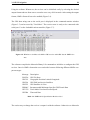
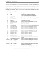
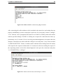
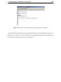
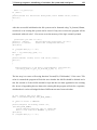
M12+ GPS receiver user’s guide chapter 5. For our application we decided for an output of
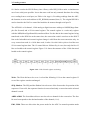
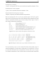
the GPRMC message once per second:
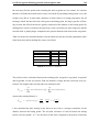
Figure 3.6: GPRMC example message
$GPRMC
154425.00
A
4342.5660
N
07216.9153
W
2.4
338.0
190105
*28
message header
UTC time of the position fix in hours, minutes, and seconds
current position fix status with A designating a valid position, and V an invalid
current latitude in degrees and minutes
direction of the latitude with N indicating North and S indicating South
current longitude in degrees and minutes
direction of the longitude with W indicating West and E indicating East
current ground-speed in knots
current direction, referenced to true North
UTC date of the position fix
checksum
Table 3.2: GPRMC message.
The M12+ receiver is used with the backup battery which is not necessary, but useful for saving setup information, especially the data output format and increasing the speed of satellite
acquisition and fix determination when the receiver is powered up after a period of inactivity. Battery equipped M12+ receivers are fitted with rechargeable 5 mAh cells, sufficient for 2
weeks to a month of backup time, depending on temperature. To recharge the cell, the receiver
must be powered up, a complete empty battery needs up to 24 hours of charge time. If set to
default, the receiver can be configured with the software again.
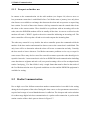
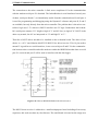
The GPS receiver is connected to the alternate RS232 pins for serial port C on the Jackrabbit
(J5). (rxc = pin4, txc = pin6, gnd = pin9) The connector for the receiver is a standard 9-pin
serial connector and wired as shown.
3.1 GPS Navigation
22
Figure 3.7: Connector M12+
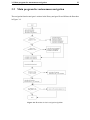
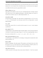
3.2 Main program for autonomous navigation
3.2
23
Main program for autonomous navigation
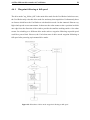
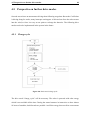
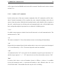
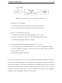
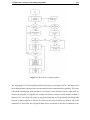
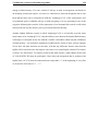
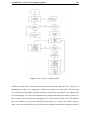
The navigation function navigate is written in the library navigate.lib and follows the flowchart
in Figure 3.8.
Figure 3.8: Flowchart for basic navigation algorithm
3.2 Main program for autonomous navigation
24
The navigate function is the heart of the navigation algorithm. It is a function called from
the drive mode "wp_follow_full()" or the drive mode "wp_follow_partial()" in certain time
distances. It makes the decision for a course correction (see chapter 4.4 for description of
drive modes).
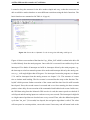
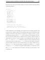
The NMEA-GPS data string is assigned to the function and the data string has to be parsed.
Therefor the function "gps_get_position" in the gps.lib is called. The function compares the
string header with the known NMEA messages, in our case "$GPRMC". If the header does
not match any of the known messages, the function returns -1 as value. If the GPS data string
is not valid, because the receiver is not tracking enough satellites, the function returns -2. If
the header is known and the data string is valid, the function now parses the position data and
stores it in a variable with the structure "GPSPosition" defined in the gps.lib. The structure
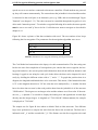
"GPSPosition" consists of:
(int)
(float)
(char)
(int)
(float)
(char)
current_pos.lat_degrees
current_pos.lat_minutes
current_pos.lat_direction
current_pos.lon_degrees
current_pos.lon_minutes
current_pos.lon_direction
Table 3.3: Sample structure GPSPosition current_pos.
That makes an easy access to the integer part of the latitude and longitude possible: "current_
position->lat_degrees" .
The most important thing for the navigation algorithm is a correct transmission of the GPSdata string. There can be all different kinds of problems in parsing the correct GPS-position.
To exclude the most transmission errors, the function to parse the NMEA-data string "gps_get
_position" makes some comparisons. Programmed from Z-World was the checking of the
header which are the first 6 characters. They also checked if the incoming string contains any
valid GPS position data or if the number of satellites did not suffice for a position determination. I also implemented a comparison of the directions of latitude and longitude. If the
header is not one of the known NMEA formats or if the NMEA-data is invalid, the navigation
3.2 Main program for autonomous navigation
25
algorithm will try to get a valid reading of GPS-data once every second until it succeeds. In
the case of not having any valid readings for 30 seconds, adjusted by "GPS_inv_limit" the
robot will change into manual drive mode without driving any distance. In that case a notice
of "GPS parsing error" or "GPS sentence invalid" will be sent out to the modem. This notice
will also be sent if one of these errors occured once but the robot will start navigating once
received valid GPS-data.
If the current position was parsed properly, the active waypoint is selected from the array of
waypoints given by the user. At startup the function recognizes that it was called for the first
time if the variable "wp_start" is 0. Then the initial distance to the active waypoint in km
is calculated with the function "gps_ground_distance" in the gps.lib. With the distance from
startpoint to first active waypoint, the bearing to that waypoint in true degrees is calculated.
A bearing value of 360◦ or 0◦ means the robot is heading to the geographic North Pole and
180◦ means the robot is pointing to the South Pole. Once in Antarctica, CoolRobot will have
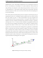
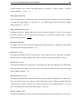
waypoints with a distance of 50 km or more. To assure that the offset from the track to each
waypoint does not increase beyond a limit, basing points are generated in a predetermined
distance to each other on the track from waypoint to waypoint. The distance to basing point
"dist" is calculated in the "navigate" function at startup. The distance to the active waypoint
is divided by 1000 m and the result is rounded off to an integer. The initial distance is then
divided by that integer and will give a distance between basing points close to 1000 m. That
calculation is made to make sure that there is a whole number of basing points between two
waypoints and that the last basing point is the waypoint.
Figure 3.9: Basingpoint and waypoint example ( drawing)
3.2 Main program for autonomous navigation
26
The last thing done in the startup procedure is that 1 is added to wp_start, so that the function does remember it’s starting point. If the navigation algorithm was called for the first
time ("wp_start == 0"), the current position saved in "current_pos[1]" is also saved in "current_pos[2]. These two positions are used to calculate the robot‘s bearing. They are the traveled positions 30 seconds apart in time wheras the time is an adjustable parameter (tm_nav).
For running through the navigation algorithm for the first time, there is no current position
from the last navigation cycle. I had two different ideas of how to proceed on the startup in
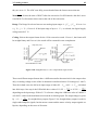
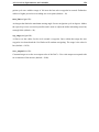
drive mode "w_follow_full". The first one is to place the robot pointing north. The current
distance at startup is 0 km and the calculated bearing between the two sample points is also
0. So at startup Cool Robot thinks his heading is north and makes a turn for the off bearing
degrees between -90◦ and 90◦ depending on the initial bearing. If the robot‘s heading is north,
in the best case the turning to the desired heading takes one navigation cycle as outlined in
Figure 3.10.
Figure 3.10: Startup procedure 1 with Cool Robot pointing north
In the worst case, the robot is pointing south instead of north at startup. That will not cause
serious problems, but takes some more navigation cycles to head to the desired course to the
waypoint or basing point as shown in Figure 3.11.
3.2 Main program for autonomous navigation
27
Figure 3.11: Startup procedure 1 with Cool Robot pointing south
The dimensions for the whole course correction procedure look larger than they are. Compared to the distance to the waypoint, the distance for the offset from the track caused by a
south pointing at startup is only about 0.5%.
The second method to proceed during startup is to take the GPS-position first and parse it for
current point[2]. Then the robot will speed up and drive straight ahead for x seconds, defined
with "tm_nav" and then it will take the current position[1] and start the first navigation cycle
as outlined in Figure 3.12. The advantage of the second method is, that the robot does not
make any useless turns that are wrong, because it does not know its heading. The idea behind
that is, that there will be a lot of interruptions forcing the robot to switch the drive mode from
"wp_follow_full" to "high_wind_speed" or "high_centered". As the robot changes its heading
in one of the different drive modes, it has no precise information on the current bearing without
any movement once back in drive mode waypoint following at full speed or partial speed. To
keep the number of navigation cycles to turn into the desired bearing as small as possible,
method two is implemented in the naviation algorithm at this point. If the robot switches the
drive mode to waypoint following it may drive 30 seconds in the wrong direction but recovers
that at the first navigation cycle instead of possibly turning to the wrong direction.
3.2 Main program for autonomous navigation
28
Figure 3.12: Startup procedure 2 with Cool Robot pointing south
The function to make course corrections is open loop. That means there is no feedback during
the turning itself. This is due to the impreciseness of the bearing information and the lack
of a compass (see chapter 3.1). But the open loop correction meets the requirements for our
project. What are 10 m on a whole continent of ice?
For the course correction, I measured the time it takes the robot to make a 360◦ turn while
driving the motors on one side at only 90% speed instead of 100% for waypoint following at
full speed and one side at 50% instead of 60% for waypoint following at partial speed. That is
possible because the motorcontrollers are setup in velocity mode. That means they try to keep
the motor at the desired speed by drawing more current.
For example, if the initial bearing to the first active waypoint is 230◦ , the function calculates an
off bearing of -130◦ without taking the robot‘s current heading into account. The off bearing
range is converted from 0◦ ≤ α ≤ 360◦ to −180◦ ≤ α ≤ 180◦ with a negative value
causing a left turn and a positive value causing a right turn and a bearing is generally measured
clockwise. To avoid imprecise turning angles, I limited the maximum turning angle for one
3.2 Main program for autonomous navigation
29
navigation cycle to 90◦ .
The current position after finishing the turn is stored and parsed into current point[2] for the
next navigation run. The robot now travels straight ahead for 30 seconds to start the next
navigation cycle with current point[1]. The distance between current point[2] and current
point[1] is calculated to determine the current bearing. Traveling with a maximum speed of
1.25 m/s, the distance should be greater or equal 30 m. That is accurate enough for the gps
receiver’s position data.
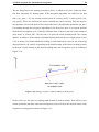
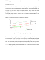
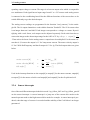
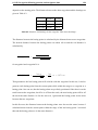
Figure 3.13 points out the necessity for basing point generation.
Figure 3.13: Example startup navigation (drawing)
The current bearing on navigation cycle 2 is almost equal to the bearing to the active waypoint,
but varies from the bearing to the basing point. If the robot would head to the waypoint, no
course correction would be made and the robot would travel on a path parallel to the calculated
track. With basing points, the traveled path is more predictable because the robot makes more
course corrections towards the calculated course. If the robot reaches a distance of less than
20 m to a basing point, the next basing point on the track is generated and the robot follows
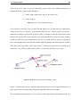
that new bearing (Figure 3.14).
3.2 Main program for autonomous navigation
30
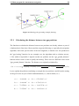
Figure 3.14: Basing point generating example (drawing)
3.2.1
Calculating the distance between two gps positions
The function to calculate the distance between two positions was already written, as part of
a diploma thesis. But when I first tested the waypoint following or especially the navigation
algorithm, with some special values of the two longitudes, a domain error was produced in
the "gps_bearing" function. In one example case, the algorithm tried to calculate arccos(1.238) which is impossible. I figured out that one problem was the "gps_ground_distance"
function whose result is used to qualify the bearing. There were two different errors in the
"gps_ground_distance" function. The distance was originally calculated by
r
lona − lonb 2
lata − latb 2
dist = 2·arcsin( cos(lata ) · cos(latb ) · (sin(
)) + (sin(
)) ) (3.1)
2
2
Let me explain the problem considering as example the two positions a and b from the testing
on the golf course on jan/11/2005 in dd.mmmmmm (alat ) and in radian (lata ):
alat =
43.428442◦ ⇒
lata = 0.76295445 rad
blat =
43.428420◦ ⇒
latb = 0.76295381 rad
alon =
72.170198◦ ⇒
lona = 1.26158792 rad
blon =
72.170212◦ ⇒
lonb = 1.26158832 rad
3.2 Main program for autonomous navigation
31
whereas radian is lata = (alat.degrees + alat.minutes /60)/180 · pi. In dynamic C the numbers
lata , etc. are defined as IEEE standard 32 bit floating points.
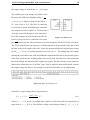
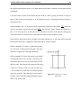
Figure 3.15: Precision for decimal values
The range for floats is not a problem, because the exponent is a signed integer in the range of 126 to 127. But if there are no leading zeros, the expansion is rounded off at the 23rd digit after
the binary point. Which is equivalent to
1
4194304
or 2.38419−7 . The problem with equation 3.1
is was not that it is false, but that it is not precise enough for our navigation algorithm, because
it tries to compensate for not having double precision floats. The fact was, that dynamic C does
not provide a data structure with double precision, like C++ or C. A library with a structure
with almost double precision was found(see chapter 3.2.3) and I developed the formula for a
distance calculation on earth based on spherical coordinates.
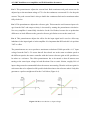
For a correct calculation of a distance
between two positions on earth, the latitudes and longitudes need to be converted into azimuth and pole angle. To
accomplish a range for the azimuth angle (ϕ) of
−180◦ ≤ ϕ ≤ 180◦
and
−90◦ ≤ Θ ≤ 90◦
Figure 3.16: Spherical coordinates
3.2 Main program for autonomous navigation
32
for the pole angle (Θ), I do the following transformations in the source code:
Θ=
ϕ=


−lati
for direction = ‘S‘

+lati
for direction = ‘N ‘


−loni
for direction = ‘E‘

loni
for direction = ‘W ‘
(3.2)
(3.3)
For latitude and longitude on earth, see figure 3.1. With these transformations, every position
on earth can be described by



r




f :  lona 


lata
7→
r · cos(lona ) · sin(lata )


 r · sin(lona ) · sin(lata )

r · cos(lata )



=



x
 
 
 y 
 
z
(3.4)
The angle α in radians between two positions on earth then is calculated with the scalar
product between the two position vectors:

cos(lona ) · sin(lata )


cos(α) =  sin(lona ) · sin(lata )

cos(lata )
 
cos(lonb ) · sin(latb )
 
 
 ·  sin(lonb ) · sin(latb )
 
cos(latb )





(3.5)
= cos(lata ) · cos(latb ) + sin(lata ) · sin(latb ) · (cos(lona ) · cos(lonb ) + sin(lona ) · sin(lonb ))
The angle α would be easy to calculate by
α = arccos(cos(lata ) · cos(latb ) + sin(lata ) · sin(latb ) · cos(lona − lonb ))
(3.6)
, but the double precision library does not include an arccos function. So I had to convert the
arccos into something known which is the arctan in this case:
arccos(α) = arctan( √
−α
) + 2 · arctan(1)
1 − α2
(3.7)
3.2 Main program for autonomous navigation
33
The distance then is calculated with the angle converted to degrees and multiplied with the
distance between two degrees.
180
km
dist [km] = α [ ] ·
· 111.136 ◦
π
◦
3.2.2
(3.8)
Calculation of gps bearing and off bearing
The function to calculate the bearing between two gps positions "gps_bearing" had to also be
transformed for a use with the "_double" precision structure and can be found in the gps.lib. It
returns the bearing in true degrees. I took the formula to calculate the bearing with knowledge
of the distance between two points a and b
bearing = arccos(
sin(latb ) − sin(lata ) · cos(dist)
)
sin(dist) · cos(lata )
(3.9)
and converted it to use double precision (see chapter 3.2.3). The arccos was substituted again
with equation 3.7.
The navigation algorithm calculates different kinds of bearings. The initial bearing is the bearing between two waypoints and marks the desired track for the CoolRobot. Initial distance and
initial bearing do not change unless the robot reaches the waypoint and heads to the next waypoint. The bearing to waypoint ("bearing_to_wp") is the bearing from the current position
of the robot to the active waypoint, same as the bearing to basing point ("bearing_to_bp") is
the bearing from the current position to the basing point. These bearings and the appropriate
distances change between two navigation cycles and are used to calculate the off bearing by
taking the difference to the current bearing ("curr_bearing"):


bearing_to_wp − curr_bearing for dist_to_wp ≤ dist_to_bp
of f _bearing =
(3.10)

bearing_to_bp − curr_bearing for dist_to_wp > dist_to_bp
The range for the "off_bearing" is −180◦ ≤ x ≤ 180◦ , whereas a negative value corresponds
to a left turn and a positive value to a right turn to correct the course.
3.2 Main program for autonomous navigation
3.2.3
34
Double precision floating point in dynamic C
Since the best way to tell the robot‘s heading is to take the bearing between the last two
positions while navigating, the single precision floating point is not precise enough for the
navigation algorithm. The distance can only be calculated exactly with the angle between two
points on earth, measured from geocenter(see chapter 3.2.1). Dynamic C does not provide a
structure double. Robert Richter wrote a double precision library on his own. We purchased
it from him. The package included the dynamic C library, his C-code, a readme file, an example file and an expression builder. This chapter presents the different functions used for the
navigation and the different commands, especially the syntax.
The double precision library creates a data type called "_double", which is internally defined
as structurechar Bytes[8]_double . The accuracy depends on the functions used:
Add, subtract, multiply, divide, and square root are all accurate down to the last bit. Add,
subtract, multiply, and divide all use 8 bits for rounding with 1 guard bit and 7 sticky bits.
Square root only has 5 sticky bits. The transandentals use C code and each term in the series
is rounded, so the multiplication and addition can result in two bit error each round. The
largest series is arctan with 22 terms, so a total of 44 operations can result in about 5 bits error
worst case.
Figure 3.17: Expression builder for "_double"
3.2 Main program for autonomous navigation
35
Figure 3.17 shows the different syntax for single float and double precision "_double". The
window shows the MFC Application to be started. The Expression builder helps to generate
source code for the new structure "_double" with the known syntax from calculations with
floats. The expression as programmed for single floats has to be entered in the "expression"
line. The expression builder has no button to create the new source code. You have to have
the "expression" line in focus and hit the enter key. The translated source code line generated
appears in the next line and can be pasted into the desired dynamic C function. The original
expression is shown after the double backslash and commented out. The variables "lata ",
"latb ", etc. can be defined as "_double = lata ", but there are functions to convert float to
double and the other way around. The most important functions are presented here to allow
an easy user interface.
_double dpMakeNum(long Num1, long Num2): Should only be used if the source code line
is generated with the PC program. This takes two long numbers and takes the bytes in the long
numbers and combines them together for the bytes in a double precision number. It is *not*
intended to be used to convert long numbers to double
_double dpFloat2Double(float Num): Converts a floating point number to a double precision
number. Note that since computers work in base 2 and not base 10, things like 0.1 become
0.1000000014901161. This is an artifact of the base 2 representation, I fill in the missing
second byte with zero’s, but the zero’s in base 2 are not zero’s in base 10.
float dpDouble2Float(_double Num): Converts a double precision number back to floating
point. This doesn’t round, so the last bit may be in error.
_double dpAdd(_double Num1, _doubleNum2): Adds two numbers and rounds the final
result. Issues with +/- infinity in the IEEE 754 format are not supported. Also, zero+very small
numbers (around 1e − 300) will cause zero to not quite be zero and may result in something
like 1.2e − 300. For numbers that aren’t at the extremes, however, zero is zero.
_double dpSub(_double Num1, _doubleNum2): returns N um1 − N um2.
_double dpNeg(_double Num): Changes the sign of a number
3.2 Main program for autonomous navigation
36
_double dpMul(_double Num1, _double Num2): Multiplies and rounds N um1 ∗ N um2
_double dpDiv(_double Num1, _double Num2): Returns N um1/N um2
_double dpSqrt(_double Num): Returns the square root.
_double dpSine(_double Angle): Sine of angle in radians.
_double dpCosine(_double Angle): Cosine of angle in radians.
_double dpArctan(_double Angle): Arc tangent in radians.
Let me just give a small example of using the structure "_double":
main(){
_double a, b, c, d, e;
float print;
e = dpMul(dpAdd(a, b), dpAdd(c, d)); //e = (a + b) ∗ (c + d)
print = dpDouble2Float(e);
printf("result of the _double calculation is: %f", print);
}
Table 3.4: Sample using structure _double.
This example ought to show the use of the double precision structure which is not supported
by dynamic C and is not known to dynamic C as a data type such as float or integer. Variables
of "_double" can be defined and used for calculations with the listed and in the "doubleprecision.lib" library written functions. If the user wants to display a number on the screen or
transmit a number to a function not listed in the doubleprecision library he has to convert the
number to a data type known to dynamic C (chapter 3.4).
3.3 Analog sensors
3.3
3.3.1
37
Analog sensors
Power and signal supplies and setup for the ADC evaluation board
The Analog Devices evaluation board eval-AD7490cb is used to read analog signals. The
AD7490 is a 16 channel, 12-bit Analog to Digital Converter. The first ADC MAX1231 from
Maxim was replaced, because we had problems with the temperature rating for their evaluation board. Any attempt to adapt the cold temperature rated ADC MAX1230, which is the
5V version of the 3.3V MAX1231 failed and support from Maxim was lacking. The second
reason for the AD7490 was that it is able to read bipolar signals that are biased at 2.5V. The
Maxim part could only read 8 bipolar channels, because it takes true differential readings from
two channels. The requirements for a Analog to Digital Converter for our project were not as
simple as evidently. The first and most important fact was the cold temperature rating of down
to -40◦ C. The box of the Cool Robot is insulated and the heat of the motor controllers should
keep the temperature always above ambient temperature, but this is the maximum rating. The
main logic is driven by two microcontrollers, one Mastercontroller for the navigation and control and one Slavecontroller for the power management, which is the work of Alex Streeter´s
master thesis. For the navigation and control side, the following analog sensors must be read:
channel
1
2
3
4
5
6
7
8
9
10
signal
motor current A
motor current B
motor current C
motor current D
motor velocity A
motor velocity B
motor velocity C
motor velocity D
tilt sensor roll
tilt sensor pitch
input range
−2V ≤ Vout ≤ +2V
−2V ≤ Vout ≤ +2V
−2V ≤ Vout ≤ +2V
−2V ≤ Vout ≤ +2V
−1.5V ≤ Vout ≤ +1.5V
−1.5V ≤ Vout ≤ +1.5V
−1.5V ≤ Vout ≤ +1.5V
−1.5V ≤ Vout ≤ +1.5V
+1.5V ≤ Vout ≤ +3.5V
+1.5V ≤ Vout ≤ +3.5V
Table 3.5: Analog input channels.
Most analog to digital converters are not able to handle negative input voltages. So we centered
3.3 Analog sensors
38
the output at 2.5V and generated a bipolar input from 0.5V ≤ Vin ≤ 4.5V . The AD7490 is
able to change the input range from 0 to Vref to 0 to 2 · Vref , where the reference voltage of
Vref = 2.5V is provided from an on-board high precision reference. The only problem was
that Analog Devices started the production of their evaluation board in February.
The power and signal supply for the ADC and the DAC is made through a 20 wire ribbon
cable (Table 3.6).
1
2
3
4
5
6
9
16
17
18
19
20
GND (DAC)
+10V (DAC)
SDI (DAC)
-5V (DAC)
CS (DAC)
CLKD (DAC)
VREF (+5V)
GND (ADC)
CS (ADC)
CLKB (ADC)
DIN (ADC)
DOUT (ADC)
DC-DC board
DC-DC board
PC0
DC-DC board
PB2
PF0
rabbit eval. board
DC-DC board
PD0
PB0
PC4
PC5
Table 3.6: ADC / DAC ribbon cable.
The on-board components of evaluation board include a programmable ultra high precision
bandgap reference and four ADG467G quad op-amps which are used to buffer the sixteen
analog input channels.
The AD7490 evaluation board is build to be used with the Eval-board controller from Analog
Devices. When using it with the Eval-board controller, all supplies are provided through the
96 way connector. When using the evaluation board as a stand alone unit, the external supplies
must be provided to the alternate pins. For connections of power supplies that are provided to
the board for interfacing the Jackrabbit microcontroller on serial port B see Table 3.7.
For using the evaluation board as a stand alone unit, +5V must be connected to VDD to supply the AD7490 and the on-board high precision reference. If interfacing the board with 3V
systems, +3V can be connected to the Vdrive pin. Usually the supply voltages for the op-amps
3.3 Analog sensors
39
digital supply voltage VDD
digital ground DGN D
analog supply voltage AVDD
analog ground AGN D
positive op-amp voltage +10V
negative op-amp voltage -5V
J7
J7
J2
J2
J3
J3
Table 3.7: EVAL-AD7490CB power supplies.
are ±12V , but the supplied voltages of -5V and +10V availablefrom the housekeeping power
distribution board on the robot are within the desired range of −18V ≤ Vneg ≤ −4.5V and
+4.5V ≤ Vpos ≤ +18V . The evaluation board has 19 switch and 19 link options to adjust
the desired functions. For operation with the Jackrabbit microcontroller the switches and links
have to be set as shown in Table 3.8.
Link No.
Function
LK0-LK15
Adds a 50. termination to AGND at the Ain0 to Ain15 sockets
(left unconnected).
Allows to user to connect a particular AD713 op-amp input to ground (H)
In position "C" an external VDRIVE supply voltage must be supplied via J7.
In position "A", the AD780 provides the 2.5V reference to the AD7490.
Adds a 50. termination to AGND at the Vin input to the Bias up circuit
(unconnected).
This link option selects the source of the SCLK input.
In position J2, the +12V is supplied from an external source via connector J3.
In position J3, the -12V is supplied from an external source via connector J3.
In position J2, the AVDD is supplied from an external source via connector J2.
S0-S15
LK16
LK17
LK18
LK19
S17
S18
S19
Table 3.8: Switch and link options on EVAL-AD7490CB.
3.3.2
12-bit, 16 channel Analog to Digital Converter on serial port B
When setup as described in chapter 3.3.1, the AD7490 can be accessed trough serial port B
using SPI.
3.3 Analog sensors
40
SPI is a three or four wire connection to shift data between two parts like a microcontroller
and an analog to digital converter. There are two connections for data input and data output
and then one for chip select and one for the serial clock. A data word transmission is started
by generating a falling edge on the chip select line CS. The following defined number of bits
are send with the falling edge of the serial clock SCLK. After the transmission, CS is pulled
high again to end the data word. Figure 3.18 shows an example conversion request on serial
port B.
Figure 3.18: Sample SPI communication on serial port B
Channel 1 is PC4, the serial data output of the jackrabbits serial port B sending two 16-bit
data words and channel 2 is the CS being pulled low for the transmission. Logic one is 3.3 V
and low is 0 V.
The problem here was, that the microcontroller has four SPI ports, A, B, C and D but dynamic
C only provides SPI library code for the use of one SPI port at a time. The desired serial port
has to be enabled to transmit data, and with the use of the SPI functions it is not possible to
enable more than one serial port. There is the possibilty to change the definition of the SPI port
in the function, but the DAC needs a logic high all the time not to update the output value.
If the SPI port would be changed to serial port B instead of serial port D for the DAC, the
output for all four motors would change to -2.9 V which is equal to a motor speed of -100%.
3.3 Analog sensors
41
So I had to rewrite the SPI.lib library into a library called SPI_B.lib to make a simultaneous
use of two serial ports possible. It uses the same code but only renamed functions for writing
to or reading from a serial port (see Table A.1in App.A). For taking readings from the ADC,
the function to write and read data is SPI_BWrRd(command, data, 2). The original SPI.lib is
used to interface the DAC to control the brushless dc motors through serial port D.
The AD7490 is a 16 channel, 12-bit analog to digital converter with up to 1MSPS(Mega Samples Per Second) and a 12-bit control register. The control register is a write-only register
with the MSB(Most Significant Bit) transferred first. For the data in the control register being
transferred on the DIN line at the same time, the conversion result is send out on the DOUT
line to the Jackrabbit each control register change is valid from the next conversion only. As
every conversion result is a 16-bit data word, it takes 16 serial clock cycles to load the new
12-bit control register data. The 12 control bits are followed by 4 zeros, but only the first 12
bits are loaded to the control register. Figure 3.19 shows the structure of the 12-bit data word
loaded to the control register.
Figure 3.19: 12-bit Control register sectioning
Write: The Write bit has to be set to 1 to load the following 11 bit to the control register. If
set to 0 the register remains unchanged.
SEQ, Shadow: The SEQ and the Shadow bits select one of the four modes of operation of the
sequencer. If set to 00, the sequence function is not used and only a conversion on the selected
channel is made.
ADD3-ADD0: The four address bits are used to select a channel for the conversion. The four
bit word corresponds to the decimal number of the channel (1-16).
PM1, PM0: These two bits select the power mode for the ADC. In normal operation mode
3.3 Analog sensors
42
they are set to 11. The ADC runs fully powered and allows the fastest conversion rate.
Weak/T RI: Selects the state of DOUT after the conversion. For SPI interface this bit is set to
0 and DOUT will return to three-state at the end of the conversion.
Range: The Range bit selects between two analog input ranges: 0 ≤ Vin ≤ Vref if set to 1 or
0 ≤ Vin ≤ 2 · Vref if set to 0. If the input range of up to 2 · Vref is selected, the digital supply
voltage must be 5 V!
Coding: Selects the output format for the 12-bit conversion result. If set to 1, the format will
be straight binary and if set to 0, the result will be returned in twos complement.
Figure 3.20: Straight binary vs. twos complement output format
These two different output formats have a different transfer characteristic for the output value
only. An analog voltage on one of the 16 channels is transferred into a 12 bit integer (0...4095).
Therefor in both cases, the full scale input range of either 0V .. Vref or 0V .. 2 · Vref is divided
into 4096 steps. One step is the LSB which has a value of 1LSB =
Vref
4096
or 1LSB =
2·Vref
4096
depending on the input range. With a 2.5 V reference voltage the LSB has a value of 0.00061V
or 0.0012V, which is the maximum error from the real analog input. The output integer is given
by code =
Vin
1LSB
for straight binary output (Figure 3.20). Straight binary output is used for
single ended unipolar signals, but the motor current and the motor velocity output signals are
bipolar, depending on the sense of direction.
3.3 Analog sensors
43
Figure 3.21: Circuit to bias bipolar signals about Vref
As the analog to digital converter cannot handle negative inputs, the signals have to be biased
about Vref . The negative full scale -2.5V is 0V and the positive full scale +2.5V is +5V. A
general circuit to bias up a bipolar input at about 2.5 volts is given in Figure 3.21. The analog
input conditioning circuit we use in our case is presented in Appendix C.
Figure 3.22: ADC DIN and DOUT with analog input signal
The DOUT line of the AD7490 shifts a 16-bit data word to the serial port B. The first four bits
indicate the information on the channel on which the conversion was requested. The next 12
bits are the digital value of the analog input voltage. The SPI port reads the 16-bit data word
3.3 Analog sensors
44
as two complete bytes which are shifted into a two dimensional character array "data[2]". A
bitwise "and" is performed with the first byte and "0F" to extract the four address bits:
0000 1111 & 0101 0011 = 0000 0011
(3.11)
The first four bits of the digital conversion result remain unchanged. At first, I thought about
programming a checksum for the address bits, to guarantee a reading on the correct channel,
but then decided to keep it simple and the communication through the serial port is correct.
3.3.3
Dual axis accelerometer used as a tilt sensor
The dual axis tilt sensor is a dual-axis accelerometer "ADXL203" from Analog Devices. The
ADXL203 measures acceleration with a full-scale range of ±1.7g. The ADXL203 can be
either used to measure dynamic or static acceleration(e.g.,gravity). By mounting different
capacitorsCx and Cy to theXout and Yout pins, the user selects a bandwith between 0.5 Hz and
2.5 kHz of the accelerometers. The part is temperature rated from -40◦ C to +125◦ C. With a 5V
supply voltage, the accelerometers have a sensitivity of 1000 mV
. The five extremal positions
g
are listed and shown below.
x1 = 2.5V ; y1 = 2.5V ; x2 = 2.5V ; y2 = 1.5V
x1 = 3.5V ; y1 = 2.5V ; x2 = 1.5V ; y2 = 2.5V
3.3 Analog sensors
45
x1 = 1.5V ; y1 = 2.5V ; x2 = 3.5V ; y2 = 2.5V
x1 = 2.5V ; y1 = 3.5V ; x2 = 2.5V ; y2 = 2.5V
x1 = 2.5V ; y1 = 1.5V ; x2 = 2.5V ; y2 = 2.5V
The accelerometers are used for the CoolRobot to detect a maximum pitch or roll angle to
prevent it from tipping over if driving while climbing large sastrugi features. An accelerometer
has a varying sensitivity in the range of -1g to +1g. The output changes with nearly 17.5 ◦mg
tilt
when the accelerometer is perpendicular to gravity but the resolution decreases and the output
changes at only 12.2 ◦mg
at 45◦ . The analog output voltage Vout : 1.5V ≤ Vout ≤ 3.5V is
tilt
converted to a range between −1V ≤ xout ≤ +1V in the function "read_sensors()" written in
the "analogin.lib" library. With 1V ⇔ 1g the output tilt in degrees can be calculated as
pitch =
out
)
arcsin( x1g
(3.12)
roll =
out
arcsin( y1g
)
(3.13)
3.3 Analog sensors
46
One thing to keep in mind is, that both outputs can exceed the output range of -1V to +1V due
to vibration or shocks by falling down a steep and sharp edge of a snow feature. To prevent
a domain error when trying to calculate the arcsin(x) for x > 1, I round the output ranges
off to 1 if they are larger. At 45◦ tilt, which is the stalling angle xout or yout has a output
of≈ 0.707V , defined as the critical tilt value (see chapter 3.3.6). To reduce the influence of
vibrations on the outputs xout and yout of the tilt sensors, a 2nd order Butterworth Filter acting
as a lowpass is integrated in the circuit. The bandwidth then is given by
BW (Hz) =
1
√
2·π· 2·R·C
(3.14)
with R = 22kΩ and C = 0.1µF , we have a bandwidth of 51 Hz. At frequencies higher
dB
. The specific feature of a Butterworth Filter is, that it
than 51 Hz, the attenuation is −40 dec
has only one cut-off frequency.
3.3.4
Motor current and motor velocity sensors
Eyes and ears of the Cool Robot, that is a good transcription for the analog sensors and especially for the motor currents and the motor velocities. The Cool Robot is powering all four
motors in velocity mode. The AMC brushless servo amplifiers try to keep the motors at the
desired revolutions by increasing the current draw for each motor if it has to provide more
torque. In reality, it is not possible to keep the revolutions at the exact same level. If the Cool
Robot climbs a sastrugi feature for example, not all wheels will reach the inclination at the
same time and one wheel has to produce more torque than the others. As a result, the current
draw for that motor increases to keep the revolution up. Meanwhile the revolutions for that
wheel drop a little and not seeing the Cool Robot or the feature that is faced, one can easily
guess what the current terrain looks like. The other way around the motor current and motor
velocity sensor for one wheel can also detect a wheel not in contact with the snow. The Cool
Robot will be confrontated with driving with one wheel in the air frequently, so that this will
not be an extreme case. But we want to be able to tell if the Cool Robot is high centered on
a large sastrugi feature or a very firm accumulation of snow with two or more wheels not in
contact with the snow.
Another reason for the motor current sensors is the very firm energy budget. The Cool Robot
3.3 Analog sensors
47
is powered by solar energy, which is a very constant and stable energy source when the sun
is shining. There will never be "too much" energy and if there is a surplus of power, then it is
nice to know for the next generation of Cool Robots. Logging the motor currents gives a very
important and highly interesting information on rolling resistance on the snow in Antarctica
and will be useful for further expeditions.
Both sensors are provided by the AMC brushless servo amplifier on the connector P1. The
current monitor output is connected to pin8 and the velocity monitor output is conncted to
pin15. The current monitor output is a voltage scaled by the factor two for each ampere current draw (1V = 2A). A positive voltage tells the user that the dc brushless motor is turning
clockwise and a negative voltage counter clockwise. The current monitor output is always
within a range of −2V ≤ Vcurr ≤ +2V due to the set current limit of the motors.
Figure 3.23: Velocity monitor out vs. motor revolution
The velocity monitor output is a periodic voltage with a rising offset for an increasing revolution. The output scales with 1V per 120 Hz Hall frequency. At a maximum revolution of
5000rpm and a number of four poles, the maximum velocity monitor output voltage is:
Vvel =
3.3.5
5000rpm
· 2 · 1V = 1.388V
120Hz · 60sec
(3.15)
Function to process the sensor data
It is one part to adjust the range for an analog signal, to build the conditioning circuits and
make the correct connections. But reading out the analog to digital converters output is another. This section describes the data processing from the 12 bit integer value to the corre-
3.3 Analog sensors
48
sponding output voltage or current. The target is to have an output value which is comparable
to a multimeter. Each signal has an input range from 0V to +5V because each analog sensor
is connected to the conditioning board. But the different functions of the sensors have to be
scaled differently to get the desired output.
The analog sensor readings are programmed in the function "read_sensors()" in the analogin.lib. The 16 output channels are read with the function "ReadAD". The 12 bit return value
is an integer between 0 and 4095. Each integer corresponds to a voltage or current. By multiplying with a scale factor, each output can be adjusted separately. Each scale factor has to
5
convert the integer to the chosen input range for the ADC of 5V by voltage = output [i]· 4096
. Then each scale factor for the analog sensor‘s output has to be multiplied. For the motor current that is 2, because the output is 1V for 2amp motor current. The motor velocity output is
1V for 120Hz Hall frequency and the tilt output is 1V for 1g. The final output values are given
below.
motor current [A]
=
5
4096
· 2 · intvalue [A]
motor velocity [RP M ]
=
5
4096
·
tilt angle [◦ ]
=
5
4096
120·60
2
· intvalue [RP M ]
(3.16)
· intvalue [◦ ]
Used in the interrupt function are the output[0] to output[3] for the motor currents, output[4]
to output[7] for the motor velocities and output[8] and output[9] for the tilt pitch and roll.
3.3.6
Sensor interrupts
One of the two different interrupts in the drive mode "wp_follow_full" and "wp_follow_partial"
are the sensor interrupts. A sensor interrupt is a jump out of the current drive mode to the
manual operator mode or the high centered drive mode for example. A sensor interrupt is produced, when the range of a sensor is exceeded and the mobility of the Cool Robot is no longer
guaranteed.
3.3 Analog sensors
49
The sensors of the robot are its eyes and all the senses it has. Two different functions are
programed for the "sensor range" handling:
1)
sensor_high_centered(int *tm_hc, int *wheel_air)
2)
sensor_range()
Table 3.9: Sensor range handling functions.
Every sensor is read once every second. The tilt sensors for roll and pitch are compared to
a limit of the value of "tilt_lim". If the absolute value for one of the tilt sensors exceeds 45◦
degrees for example, the function stops the robot. A routine to drive the robot back on the
driven track is called. The motor speeds are set to backwards 100%. After 4 seconds, it makes
a right turn with 90% speed compared to 100% for 18 seconds which is equal to a 60 degrees
turn. After that the robot will stop and continue with navigating at the desired speed. If called
from drive mode "wp_follow_full" (drive_mode = 1) the motor speeds are set to 100% and if
called from "wp_follow_partial" (drive_mode = 2) the motor speeds are set to 60%.
Figure 3.24: High tilt angle interrupt handling sample
Figure 3.24 shows the track of a high tilt angle interrupt. After the motor speeds have been set
to the speed before interrupted the navigation algorithm will start over again.
The second function checked once every second, is detecting a high centered position. In case
3.3 Analog sensors
50
of one wheel being without contact to the snow, the current will drop to the no-load-current
value. The motor velocity will increase a little to almost the maximum revolutions. That only
is not a criterion to detect a high centered position, because the Cool Robot will travel with
only three wheels in contact to the snow repeatedly. What I am doing is, i check all four wheels
once every second for a current value that is close to the no-load current value. If that is the
case, I check the motor velocity as well. If the motor velocity is above 4950 rpm , I log the
tilt angles. The number of the wheel is stored and this wheel is checked again after a second.
If the current is still low and the revolutions at a high level, the tilt angles are read out and
compared to the first reading. After 10 readings of a very low current, a high speed and almost
no difference in the tilt angles the drive mode "high_centered" is called. In the case that the
current for the selected wheel increases to the next second, the algorithm recognizes that and
all four wheels are checked again. The drive mode "high_centered" is not implemented yet. It
is very hard to tell the best way how to get back enough propulsion for further movement. That
has to be a part for the next students. The time the robot waits after defining a high centered
position is set to 10 seconds but can be adjusted by "tm_hc".
51
Chapter 4
The overall control unit
The overall control unit of Cool Robot is one main part of the robot’s logic. It consist of the
Digital Analog Converter TLV5614, four Advanced Motion Controls brushless servo amplifier AMC BE15A8-H and EAD brushless dc-motors EAD DA23gbb-m300. The control unit
basically consists of the different drive modes for the Cool Robot. A drive mode calls the
navigation algorithm, checks the sensors, and listens for manual interrupts incoming through
the user interface radio or iridium modem. Depending on the drive mode the propulsion has
to be assured. Each drive mode checks the motor_speeds at frequent intervals and if needed
updates the DAC‘s output. The motor controllers are supplied with 48 Volts, as well as the motors themselves. The speed of each motor is controlled with the DAC‘s output. This chapter
will explain the design and construction of the DAC setup together with the motor controller.
The DAC is connected to serial port D. Table 4.1 shows all serial port connections on the
jackrabbit.
serial port:
A
B
C
D
E
F
function
programing and compiling port
analog to digital converter AD7490
GPS-receiver Motorola Oncore M12+
digital to analog controller TLV5614
radio modem
iridium modem
Table 4.1: Serial port connections and functions for RCM.
4.1 Navigation and control mode overview
4.1
52
Navigation and control mode overview
Table 4.2 summarizes the navigation and control modes assumed for the robot.
wp_follow_full
m
and navigates auThe Cool Robot drives at the top speed of 1.2 sec
tonomously to follow the given waypoints and the generated basing
points. The GPS-receiver is set to output the NMEA-GPRMC message once every second. The robot will parse its position once every
30 seconds after achieving the last course correction to calculate the
current bearing and the next off bearing. While traveling, the analog
sensors are read once every second. The wheel speeds and motor currents are compared to detect a high centering position and switch to
the drive mode "got_stuck". The tilt sensors are also interrupt driven
to prevent the robot from tipping over.
wp_follow_partial
The same routines as in the drive mode "wp_follow_full" are run,
except that the robot travels with a speed of 60%.
manual_operator
The Cool Robot is not navigating autonomously. The GPS-data
string send out to the serial port and the motor speed command to
the DAC in percent are send back to the radio modem connected to
the Laptop and are displayed in the "HyperTerminal" window. The
robot can be controled with the keypads:
w (10% motor speed increment)
s (10% motor speed reduction
a (left turn with 10% difference in motor speeds left to right)
d (right turn with 10% difference in motor speeds right to left)
q (stop: decreases all motor speeds to zero within 1 second)
p (switch to wp_follow_full: motor speeds set to zero!)
high_centered
This drive mode is accessed, when the wheel speed sensors and the
motor currents create the interrupt in one of the waypoint following
drive modes.The Cool Robot tries to get all four wheels back in contact with snow. This routine has to be evaluated during the testing in
Greenland.
4.2 12 bit Voltage output DAC with serial interface
charge cycle
53
The navigation is reduced to parsing the GPS Position from the
GPS-data string. The motor controller are shut down and the power
consumption is reduced to a minimum. Accessed by the Slave controller maintaining the power overall power supply as a part of Alex
Streeter‘s master thesis.
high_wind
The robot is turned with one corner facing the wind. Energy consumption is reduced to minimum in case of a blizzard. Movement of
twice the length of the robot once in a while to prevent snowing in.
Not implemented at this time.
stat_get_data
The drive mode in which the robot mainly does nothing. The largest
part of the bandwidth is reserved for the payload data transmission.
Table 4.2: Control and drive mode overview
The main control algorithm for the Cool Robot is split into different drive modes. A drive
mode is the summarization of the basic functions needed to handle the current situation. As
the circumstances change during the robot‘s trip, the priority for each algorithm changes.
The main active program on the Master controller maintains the connection to either the radio
modem or the iridium modem (see chapter 5) and also changes the drive modes if needed (see
chapter 4.4). More drive modes are designated but not implemented yet, because the needs for
the scientific payload are not specified and the wind speed sensor is not implemented yet (see
chapter 4.4).
4.2
12 bit Voltage output DAC with serial interface
Selected for our drive train was a Digital to Analog Converter from Texas Instruments, because
they had the best support with their package. The digital supply voltage is separated from the
analog side and can be varied between 2.7V and 5.5V. The TLV5614 has 4 DAC´s with a
resolution of 12 bit and an output voltage. A 12 bit resolution says, that a voltage range, here
4.2 12 bit Voltage output DAC with serial interface
54
the output voltage is divided into 212 = 4096 steps.
The smallest part each voltage step differs from
the next is the LSB(Least Significant Bit) =
1
4096
·
(voltagerange). Supply voltage for the part is ±
5V. VREF is set to 10 V. The DAC is connected
to serial port D on the Jackrabbit main controller
(for connections refer to Table 3.6). The four DAC‘s
are easily accessable through a 3 wire serial interface (SPI) using the provided code for the SPI.lib.
Figure 4.1: SPI Interface
If there is only one device connected to the serial
port, CS can be tied low. The maximum serial clock frequency for the TLV5614 is 20 MHz.
The FS pin is the Frame sync input pin. A falling edge has to be generated on this pin to shift
the data in the serial output to the DAC, where the minimum high-level digital input voltage
for DVDD = 5V is 2.2 V and the maximum low-level is 0.9 V . The falling edge on FS starts
shifting the 16-bit data word, with the MSB(Most Significant Bit) first to the internal register
of the DAC clocked by the 16 falling edges of the serial clock. After FS rises or the sixteen bits
have been shifted, the addressed DAC updates the output. The data consists of four control or
address bits followed by the 12-bit DAC value. DACA, which is addressed by 0000, controls
the output voltage for motor A for example (see the drive.lib header for all address bits).
Figure 4.2: DAC 16-bit data word
Each DAC‘s output voltage then is represented by
Vout = 2 · Vref ·
DAC value
[V ]
4096
(4.1)
where Vref = 2.5V in our case and the DAC value the 12-bit data word to be transfered in a
range from 0 ≤ x ≤ 4095 is. The reference voltage can be adjusted from 0V ≤ Vref ≤ 3.3V
4.3 AMC brushless servo amplifier and EAD brushless dc motors
55
with the potentiometer on the DAC board. To buffer the DAC‘s ouput signals, we connected
an Opamp LM248 to the output channels.
The final output voltage range is outlined in Figure 4.3.
Figure 4.3: Voltage output vs. digital input
4.3
AMC brushless servo amplifier and EAD brushless dc
motors
The motor controllers are PWM (Pulse Width Modulation) servo amplifiers of the model
AMC BE15A8-H. Supplied with 48V, the amplifier can be interfaced with a digital controller
or used as a stand alone unit. The amplifier is controlled by the quad voltage output DAC from
Analog Devices. Various switches and potentiometers allow the user to adapt the amplifier to
the existing system and to synchronize the four amplifiers.
The four switches are set up for velocity mode with the parameters to adjust with the potentiometers.
The function of the four 14-cycle potentiometers are outlined below:
Pot 1: This potentiometer adjusts the loop gain in velocity mode. The loop gain increases
while turning clockwise. For the Cool Robot it is turned fully clockwise.
4.3 AMC brushless servo amplifier and EAD brushless dc motors
56
Pot 2: This potentiometer adjusts the current limit. Both continuous and peak current can be
adjusted up to the maximum ratings of 7.5A for the continuous current and 15A for the peak
current. The peak current limit is always double the continuous limit and at maximum when
fully clockwise
Pot 3: This potentiometer adjusts the reference gain. This means the ratio between input voltage from the DAC and output velocity is increased by turning the potentiometer clockwise.
Not every amplifier is turned fully clockwise for the Cool Robot, because due to production
differences or load differences the general reference gain limits are not at the same level.
Pot 4: This potentiometer adjusts the offset for the input signal and is used to offset any
imbalance in the input signal or in the amplifier. It is important that DIP switch 4 is in position
"Off" or offset.
The potentiometers are set to produce a maximum revolution of 5000 rpm with a ±3V input
voltage from the DAC‘s. To assure that all four wheels are at the same revolution speed at
the different speeds, the motor controller with the lowest reference gain at full speed has to
be taken as a reference. The offset potentiometer has to be turned so that all motors start
turning at the same input voltage in both directions. Due to static friction, roughly 20% of
input voltage must be commanded before the motors start turning. Then the reference gain for
each motor has to be adjusted at full speed in both directions to the reference wheel. Only this
guarantees a perfect straight track for the Cool Robot (Figure 4.4).
Figure 4.4: Motor revolutions vs. input voltage
4.4 The different drive modes of Cool Robot
57
As shown in Figure 4.4 the output voltage is not linear to the wheel speed. The drawing on the
right side shows how the motor speed behaves compared to the input voltage provided from
the DAC.
The brushless dc motors DA23-DBB-M300 from EAD-Motors are mounted to the gearhead
with a 100:1 ratio. A maximum revolution after the gearhead of 50 rpm and a tire diameter of
20 inch provides a top speed of
Vmax =
4.4
50rpm
10inch · 2.54m
m
·2·π·
= 1.33
60sec
100
s
(4.2)
The different drive modes of Cool Robot
On the trip over the Antarctic Plateau the Cool Robot has to face many different situations.
Some algorithms and functions have a different priority during the trip. The best example is
the navigation algorithm. Most of the time the Cool Robot will be following waypoints on
the Antarctic Plateau, but if the power budget runs low the robot has to stop to recharge the
li-ion batteries. Once standing at one position without driving the motors, there is no use of
calculating distances and bearings. The navigation algorithm can be "shut down". To meet
the different requirements, drive modes for the Cool Robot are implemented. A drive mode
grades and arranges the different base functions used to read the sensors, to control the motors
or to navigate for example. A detailed overview over the Cool Robot‘s drive modes is given
in Table 4.2.
The drive modes and a general description are listed below.
wp_follow_full(): In the drive mode "waypoint following at full speed" the robot travels at
m
1.3 sec
on the calculated track to the next active waypoint. High energy consumption.
wp_follow_partial(): Called from the drive mode "waypoint following at full speed" when the
Slave microcontroller sets a power limit which forces the motors to run slower. Still heading
to the waypoint.
manual_operator(in_string): Designed to have easy manual control over the robot to drive
4.4 The different drive modes of Cool Robot
58
it into a garage instead of carrying it. Highest priority and interrupt driven in all other drive
modes. Control via keypad (w-faster, a-left, s-slower, d-right, q-stop).
high_centered(in_string): Detected and called by the motor current and motor velocity sensors if the Cool Robot is high centered. A routine that turns the wheels forward, backward,
turns left at -100% and +100% to get the Cool Robot unstuck again.
charge_cycle(): Accessed only from the drive mode "wp_follow_partial" if the power budget
allows no further propulsion. Parameters have not been selected at this point and need to be
set by the Slave microcontroller appropriate for the energy consumption.
high_wind(): A drive mode that has to be implemented once the wind speed sensor is attached.
m
. Should prevent the
Will turn the robot into the direction of the wind at high speeds ( ≥ 20 sec
robot from tipping over because it is facing the wind from the side or being tilted at one corner
so that the wind is able to get under the robot. Should also move the robot a few meters to
prevent it from getting snowed in.
stat_get_data(): The Cool Robot has a scientific assignment. To take measurements it has to
stay on one position. In that case the bigger part of the bandwidth of the iridium communication is reserved for the payload for example.
4.4 The different drive modes of Cool Robot
4.4.1
59
Waypoint following at full speed
The drive mode "wp_follow_full" is the main drive mode for the Cool Robot. In the best case,
the Cool Robot only exits this drive mode for stationary data acquisition. Unfortunately there
are factors which force the Cool Robot to exit that drive mode. On the Antarctic Plateau very
high wind speeds are not uncommon. In that case the robot wants to take a position in which
one edge faces the direction of the wind to provide the smallest working surface. One other
reason for switching to a different drive mode such as waypoint following at partial speed
could be a power limit. However, the Cool robot starts in drive mode waypoint following at
full speed after powering up in manual drive mode.
Figure 4.5: Flowchart of drive mode waypoint following at full speed
4.4 The different drive modes of Cool Robot
60
I wanted to keep the structure for the drive modes simple and easy, so that the next users are
able to add drive modes that have to meet different restrictions using the basic functions. The
basic functions are summarized in Table A.1(App.A).
Figure 4.6: Screen shot of dynamic C code for waypoint following at full speed
Figure 4.6 shows a screenshot of the function "wp_follow_full" which is written in the drive.lib
is called directly from the main program. Once called it is executed in an endless loop if not
interrupted. Two kinds of interrupts are build in, interrupts driven by the main program, e.g.,
the interrupt to switch to manual operator drive mode and interrupts driven by the analog sensors, e.g., a tilt angle higher than 45 degrees. For interrupts from main program, see chapter
5.3.4. and for interrupts from the analog sensors see chapter 3.3.6. The structure of costate
tries to imitate multi tasking. The first costate is executed but the stops at the function "DelayMs" which prevents further execution of the costate until the time listed in milli seconds
has elapsed. If not, the second costate is executed and so on. Once running, the three costates
produce a time delay for an execution of the commands listed behind each costate. In this case,
the GPS-data string from the Motorola GPS-receiver is read, the motor speeds are checked if
at full speed and the analog inputs are read once every two seconds. The interrupts for high tilt
or a high centered position are checked once every second. Then, after the defined navigation
cycle time "tm_nav" (30 seconds) has elapsed, the navigation algorithm is called. The robot
will now parse its current position, correct the course if necessary and will return back to the
4.4 The different drive modes of Cool Robot
61
main loop after that.
The drive mode "wp_follow_full" sets the paramaters for the navigation based on GPS-data.
It defines the distance between two navigation cycles which has to be aligned with the desired
precision, the available GPS-precision and the distances to travel. If the robot navigates once
every 10 seconds it will make a lot of course corrections and the track will look like a sawtooth.
If the time between two navigation cycles is larger then 30 seconds for example, the algorithm
will smooth the track by taking shifts in bearing caused by the terrain into account.
The drive mode also includes the only obstacle avoidance of the robot: high tilt angles. The terrain in the Antarctica is mostly flat and obstacles like mountains or crevasses can be detected
on satellite images. The waypoints given to the Cool Robot force it to avoid these obstacles.
The sastrugies sculpted by the wind have to be handled. Therefor we have the tilt sensors. The
slow speed of the robot allows us to stop it, back it up and drive around the feature if it would
be dangerous to climb it.
During waypoint following at full speed, the robot checks the tilt angles , the motor speeds and
the motor velocities once every second. If one of them is out of the range, the robot is stopped
and the drive mode is changed. After driving around a high tilt angle or after getting out of a
high centered position, the robot will start the drive mode "wp_follow_full" again. The same
routine as described for the startup is executed to get back on the defined track (chapter 3.2).
During the whole time the robot is driving in "wp_follow_full" it can be interrupted and
switched to the drive mode "manual_operator" by sending the command "$CRCMDMANDM"
from the modem (chapter 5.3.4).
4.4.2
Waypoint following at partial speed
The drive mode "wp_follow_partial" is implemented to guarantee a movement if the energy
budget does not allow to drive the motors at full speed. The motors are driven at 60% of the
m
maximum speed which is equal to a speed of 0.78 sec
. The drive mode will be called by a
routine from the Slave microcontroller which handles the overall energy consuption and bud-
4.4 The different drive modes of Cool Robot
62
get. The main algorithm is the same as described in chapter 4.4.1. The difference to waypoint
following at full speed is, that the time between the navigation cycles is defined for two different situations. If the drive mode is accessed through power restrictions, the navigation time
is set with "tm_nav_low" which is longer than in waypoint following at full speed, because
the robot needs more time to travel the same distance. The same shape of the track should
be achieved. To have the same distance between current position[1] and current position[2],
"tm_nav_low" is calculated automatically to
tmnav low [sec] = 1.67 · tmnav [sec]
The drive mode "wp_follow_partial" is also accessed if the Cool Robot reaches the last waypoint within a certain distance. Then the robot is slowed down and the time between two
navigation cycles is short to allow the robot to get very close to the waypoint. If navigating
with full speed, the distance between two navigation cycles is greater than 30 m. That makes
it hard or impossible to reach a certain point within a range of 10 m. So the robot changes
to partial speed once within a range of 100 m of the last active waypoint in the list. The time
between two navigation cycles is set in "tm_nav_wp" and set to 10 seconds.
4.4.3
Manual Operator
The drive mode "manual_operator" gives the user the ability to control the robot manually
with the keypad of a laptop or computer with radio connection within a range of 1.2 km (0.78
miles). Is implemented to be able to drive the robot out of a garage for testing or any other
purposes. The functions for the manual control are written in the drive.lib. They split the range
of negative full speed to positive full speed into 20 steps. Every hit on the keypad is equal to
a 10% change of the motor speeds. The robot is accessed with the five keys w, a, s ,d, q.
w: All four motor speeds are increased by the value of "motor_speed_increment" which is
10% in default as long as none of the four already is at full positive speed. If the robot is
driving backwards, an increase of the nagative value will force it to go slower backwards. If
the commands are sent through the radio connection, more then one key can be sent at one
time. A string of ten times "w" should be avoided, since the stress on the motor, the gearhead,
4.4 The different drive modes of Cool Robot
63
the support tubes and the axes is very high then because there is almost no delay between the
commands.
s All four motor speeds are decreased by the value of "motor_speed_increment" as long as
none of the motor speeds already is at full negative speed. If driving forward, the robot is
decelerated 10%.
a By sending the key "a" the motor speed A and motor speed B are decreased
speed C and motor speed D are increased
angle
.
2
angle
2
and motor
The variable "angle" defines the radius for a
turn , if "a" was sent once. As the robot is skid steered, it can turn on one place by driving one
side of the wheels at 100% positive speed and the other at 100% negative speed.
If the robot is driving forward it will make a left turn with the key "a" but if the robot is driving
backwards it will make a right turn as the direction of "front" changes.
d The command "d" makes a right turn instead
of a left turn if driving forwards and a left turn
instead of a right turn if driving backwards.
q The command "q" forces the robot to stop within
a maximum time of two seconds. It decreases all
four motor speeds by 10% in a time delay of 200
milli seconds. That means if driving with full speed,
it takes 2 seconds to come to a full stop but only
1.167 seconds for a full stop if driving at partial
speed for example. This function is also used to
stop the robot if detecting a high tilt angle in drvie
mode "wp_follow_full".
Figure 4.7: Overview of motor
placement
4.5 Perspective on further drive modes
4.5
64
Perspective on further drive modes
Our task was to have an autonomous driving robot following waypoints. But as the Cool Robot
is driving along for weeks, many interrupts can happen. A blizzard can force the robot to turn
into the wind, or force it to stay at one point to recharge the batteries. The following drive
modes need to be implemented in the system in the future.
4.5.1
Charge cycle
Figure 4.8: Drive mode charge cycle
The drive mode "charge_cycle" will be necessary. The robot is powered with solar energy
which is not available all the time. During the austral summer in Antarctica we have almost
18 hours of sunshine, but blizzards are possible. And if the energy does not allow a movement
4.5 Perspective on further drive modes
65
at all, the energy consumption has to be reduced to a minimum to recharge the batteries with
the available sun power. The robot should be still able to read the sensors such as wind speed
to turn into the direction of the wind and should still have a connection to the user for a status
request for example. A possible configuration could be the routine in Figure 4.8.
4.5.2
Stationary data aquisition
Figure 4.9: Drive mode stationary get data
The parameters for the scientific payload have not been specified yet. But as measurements
have to be taken stationary, the robot changes into a drive mode, which is similar to "charge_
cycle", except that some energy is used for the payload and that most of the bandwidth is
reserved for transmitting scientific data. A possible routine is pointed out in Figure 4.9.
4.5 Perspective on further drive modes
4.5.3
66
High centered
This drive mode is possibly the hardest to predict. The idea behind it is to get the robot back to
navigating again once it is high centered on a large feature with two or more wheels with not
contact to the snow. The Cool Robot has a ground clearance of 23 cm which is not large, but it
could handle all the terrain during the tests on mascoma lake. Sastrugi features have one sharp
edge with slopes of not larger than 40◦ . If the other side rises slowly, that is only a problem if
the robot drives parallel to that edge with one side of the wheel at the lower end and one side
driving on top of the sastrugi. If the feature rises rapidly, the robot will simply drive against it
like it is an obstacle and will not make any movements although the wheels are turning. The
currents will not drop and the motor velocities will not go up. The way to detect that will be a
task for the next students.
To detect a high centered position is already implemented in one of the interrupts. The robot
is stuck in a high centered position, if it is centered on a high feature with the bottom of the
chassis and two or more wheels with no contact to the snow. It is not able to drive on. The
sensors for motor currents, motor velocities and tilt angle detect this situation and the drive
mode "high_centered" is called to get all four wheels back on the snow. This has to happen
by designing a method to turn each wheel in a different direction and use the weight of the
wheels to force the robot to slide to one side and be able to drive back off that feature.
At the moment I have written a routine that tries to drive the robot backwards off that obstacle
and tries to turn one side of the wheel forwards full speed and the other side backwards.
67
Chapter 5
Communication of CoolRobot
According to the overall concept of the Cool Robot it should basically be able to travel
autonomously along a predefined track on the Antarctic plateau. The track will be defined
through an arbitrary number of waypoints that consist of GPS coordinates. Those can be implemented in the control algorithm of the robot before it starts its journey.
So why communication between robot and base? There are a number of different reasons for
a communication system. The first and most important is the ability to alter the course of the
robot once it is started. At some point it might be essential to have the opportunity to stop the
mission and make the robot return to its base immediately. In other cases one may want to add
points to the route to take extra measurements, or just alter existing waypoints anticipating
possible problems on the planned route. Another argument is the fact that the robot might get
into some critical situation. Although the terrain on the arctic plateau is supposed to be quite
even it is possible to get stuck on one of the Sastrugi features. Some testing on hard snow with
features like those on the Antarctic Plateau showed that there is a possibility to get stuck if
the robot runs longitudinal onto one of those features. In that case the robot must be able to
realize it is stuck, which is part of the navigation process, try to get itself unstuck and if this is
not possible it has to send a status report back to the base. This report must contain at least the
position at which the robot got stuck to be able to pick it up. It might also be useful to have
all other available sensor data to get an exact idea of the situation. With enough information
about the actual situation of the robot it might be possible to free it by driving manually or
5.1 IRIDIUM Communication
68
with a special set of commands to move it based on the momentum of the wheels.
There are lots of other possible errors imaginable that could force the robot to stop. For example, problems with the power system, low batteries, burned fuses or other hardware or
software-related problems. Finally it might be necessary to know where the robot is and in
what condition. It is quiet possible that the robot is not going as fast as is supposed to and
therefore is not able to finish the planned route within the time alloted for its mission. So, it
is important to check the progress periodically and be able to alter the track or cover extra
distance if it is ahead of schedule. Depending on the kind of scientific application of the Cool
Robot, it might also be necessary to send some of the measured data to base.
5.1
IRIDIUM Communication
Within the concept development of the robot the decision was made that an IRIDIUM modem
shall be use for the data-communication in the Antarctic. Iridium is a global satellite based
cell phone technology. At the moment, IRIDIUM is the only provider of satellite voice and
data solutions with coverage of nearly the whole surface of the earth including all oceans,
airways and also the arctic and Antarctic region. Due to the long distances of several hundred
kilometers the robot is covering IRIDIUM is the only way to stay in touch with Cool Robot.
Since Cool Robot is a lightweight construction there is no possibility to use big, heavy radios
with the range needed in this application. Another argument for not using such a radio is
the power consumption and power output, since this may affect the electronics controlling
the robot and also the measurements of the carried payload. The big advantage of IRIDIUM
technology is its global availability and the fact that it makes no difference if the operator is
also in the Antarctic or somewhere else in the world. The disadvantage is the high price and
slow bandwidth of 2400Bit/s. According to this, there will be no permanent connection but
rather only data-transfer when needed. Therefore, either the robot or the operator will have to
establish the connection. Figure 5.1 provides an example IRIDIUM application.
5.1 IRIDIUM Communication
69
Figure 5.1: Example for an IRIDIUM modem application
The IRIDIUM System was developed by Motorola in 1980 as a personal communication system for users that need communications access to and from remote areas where no other form
of communication is available. It consists of 66 operational low altitude satellites grouped into
six polar planes of 11 satellites. Each of the satellites performs as node of the telephony network. 13 additional satellites act as backup system. The satellites circle the earth once every
100 minutes in a near polar orbit at an altitude of 780km. On the surface the system comprises
system control segment and telephony gateways connected to the telephone system on earth.
The uplink to the satellites uses TDMA and FDMA multiplexing methods. TDMA reads Time
Division Multiple Access which is a technology for delivering digital wireless service using
time-division multiplexing (TDM). The radio frequency is divided into time slots which are
then allocated to multiple calls, so a single frequency is able to carry multiple, simultaneous
data channels. FDMA on the other hand means Frequency Division Multiple Access.
5.1 IRIDIUM Communication
70
Figure 5.2: FDMA versus TDMA
In case of IRIDIUM the frequency band is 1616-1626.5MHz and is divided into 20 channels
and each of those channels is time divided into 4 TDMA channels. This multiplies to 80
channels per cell. Considering that each of the 66 satellites has 48 cells this makes up a total
of 3168 cells. Only 2150 cells are active at a time, multiplied by 80 channels per cell the
system allows up to 172000 calls simultaneous. The bandwidth for each of the channels is
2400Bit/s when transmitting data and 4800Bit/s on a voice call.
5.1.1
The A3LA-I IRIDIUM modem
The IRIDIUM-modem or IRIDIUM Subscriber Unit (ISU) used when Cool Robot will be
deployed in the Antarctic is a Motorola 9505 A3LA-I. The unit will not be purchased but
rather borrowed for Cool Robots mission in the Antarctic. Thus, no example is available for
testing at the moment. I was only able to familiarize myself with some facts as well as the
handling and operation of this equipment.
5.1 IRIDIUM Communication
71
Figure 5.3: Motorola 9505 A3LA-I IRIDIUM modem
Other than normal IRIDIUM mobile phones this modem is special designed for the use with
computer or micro controller based applications. Using the modem alone no IRIDIUM call
can be completed because some additional equipment is needed. An antenna is required, since
the modem doesn’t come with one. Lots of different antennas for almost every requirements
are available on the market. The one preferred for our project is the NAL Research SAF2040
family of mobile flat mount antennas. They are designed to withstand harsh environmental
influences, are very small in dimension and most important the frequency range is fitted to
the the IRIDIUM requirements, which means they provide continuous coverage from 1610 1626.5MHz. The various Types of antennas of this family only differ slightly in their dimensions and electrical specifications.
Figure 5.4: SAF2040-E mobile flat mount antenna
Due to the fact that there is no input or control device included with the A3LA it must be
attached to a micro controller or computer equipped with an RS232 serial port. All commu-
5.1 IRIDIUM Communication
72
nication between the ISU and the Data Terminal Equipment (DTE i.e. micro controller) takes
place over this serial connection. Depending on the attached DTE two wiring possibilities
are given. First a full 9-wire interface, incorporating hardware handshaking and flow control
or a 3-wire interface where only ground GND, receive RX and transmit TX are connected.
Connecting the A3LA to the Jackrabbit micro controller a 3 wire interface will be sufficient,
since hardware handshaking and flow control are not essential for us and would complicate
the communication routines and especially the wiring of serial port E. Since for this kind of
serial communication no SPI protocol is used it can take place while all other systems of Cool
Robot are running. The only disadvantage of the 3 wire interface is that some settings (see
chapter 5.1.1.2) must be accommodated to this circumstances. When connecting the A3LA to
a personal computer the 9-wire interface is probably the better solution.
5.1.1.1
Using the A3LA-I IRIDIUM modem
For the control of the A3LA the the industry standardized basic (Hayes) AT command set plus
a extended AT command set is used. AT means Attention Code and signals the modem that
one or more commands are to follow. Both types of commands have different syntax to query
and adjust their settings. As these commands are industry standard language to communicate
with a modem it is used with most modems available on the market. All commands in this
language must begin with the characters "AT". The only exceptions are the repeat command
"A/" and the escape sequence "+++". Many of the basic commands consist of one single alpha
character in other cases a special character (like %, $ or *) precedes the alpha character. Most
of the extended commands use a "+" prefix plus alpha characters. For example:
Extended Cellular Commands
+C prefix - Used for GSM cellular phone-like functions (Standards: ETSI specifications GSM
07.07)
Extended Data Compression Commands
+D prefix - Used for data compression (Standard: V.25ter)
5.1 IRIDIUM Communication
73
Extended Generic Commands
+G prefix - Used for generic DCE issues such as identities and capabilities (Standard: V.25ter)
Extended Interface Control Commands
+I prefix - Used to control the DTE interface (Standard: V.25ter)
Motorola Satellite Product Proprietary Commands
-MS prefix - Proprietary to the Motorola Satellite Series product line
Both, the command prefix ("AT") as well as the command sequence itself can be typed in
upper or lower case but must not be a mix of both. Furthermore many commands can be typed
within one command line divided by spaces for better reading if desired. Figures 5.5 and 5.6
show example commands and command lines.
Figure 5.5: Some sample commands with explanation (AT manual for A3LA)
Figure 5.6: Example for different ways to type commands (AT manual for A3LA)
The only limit hereby is the size of the command line buffer which normally accepts 39
characters including the "AT" prefix. Spaces, carriage return <CR> and line feed <LF> do not
go into the buffer and therefore don’t count against the 39 character limit. In case of a syntax
error within the command line or if the 39 character limit is exceeded the whole command line
5.1 IRIDIUM Communication
74
will be ignored and an ERROR result code will be returned. Possible result codes are shown
in Table 5.11.
5.1.1.2
Outline on AT commands
In this section some of the most common commands of the AT command set will be introduced. Essential commands will be explained by some examples including result codes as
answers from the modem. With this short introduction the reader should be able to originate a
data call , switch between in-call data mode and command mode, end a call and adjust some
basic settings that might be important for use within the CoolRobot project.
"+++"
So called escape sequence switches from in-call data mode to in-call command mode. The
modems answer is "OK".
"A"
The answer command "A" forces the modem to answer an incoming call immediately.
"A/"
Repeats the last command issued to the modem unless it was reset or power was interrupted.
"A/" is not followed by a <CR>. The answer depends on the last command.
"AT"
As mentioned earlier "AT" is the prefix for all commands except the repeat instruction "A/"
and the escape sequence "+++". "AT" entered on its own forces the modem to answer "OK".
"Dn"
Is used to dial a data or voice call number. Syntax is ATDnx...x, where n is a modifier
for the dial instruction and x...x represents the number to dial. Allowed values for x are
1234567890*#ABC. The modifier alters the way the A3LA is dialing:
5.1 IRIDIUM Communication
L
P
T
+
;
>
75
redial last number
use Puls dialing
use Tone dialing
(it doesn’t matter whether Puls or Tone dialing is used)
international dial prefix
start a voice call (without this a data call is originated)
used to dial a number from the phone book
Table 5.1: Modifiers for Dn.
"En"
Determines whether characters are echoed locally. Echoing characters locally should be disabled on the CoolRobots modem (see chapter 5.2.1.2 for explanation).
n=0
n=1
characters are not echoed to the data terminal
characters are echoed to the DTE.
Table 5.2: Modifiers for En.
"Hn"
Used to hangup a data or voice call originated with ATD, ATA/ or ATS0=n answer commands.
A zero value for n places the modem on the hook.
"On"
The online command switches from in-call command mode to in-call data mode. Any value
n=0 to n=255 is allowed but does not change the effect of the command.
"S0=n"
Sets the modems S0 register, which holds the setting for auto-answering to the value n carries.
Every value higher than 0 enables the auto-answering function. n=0 disables auto-answering.
It should be a good idea to enable this setting on the CoolRobots A3LA since answering a call
manually requires an extra function or routine that can be omitted using this setting.
5.1 IRIDIUM Communication
76
"Vn"
This sets the response format the modem uses either numerical or textual. n=0 causes numerical responses whereas n=1 causes textual answers. For the use with a PC the textual (Verbose)
mode might be the better way, whereas for the use with the Jackrabbit numerical answers
might be easier to process.
"Zn"
The "Zn" command acts as a soft reset and restores one of the two available user defined
configurations. See description of "&Wn" for information on storing user defined configurations.
n=0
n=1
restore user settings profile0.
restore user settings profile1.
Table 5.3: Modifiers for Zn.
"&Cn"
This setting changes the behavior of the modem to the Data Carrier Detect signal (DCD),
which indicates whether the modem is connected to a remote station for data exchange or
not.
n=0
n=1
DCD is forced on all the times.
DCD indicates the connection status.
Table 5.4: Modifiers for &Cn.
"&Dn"
This option is used to determine the A3LAs behavior on the Data Terminal Ready (DTR)
signal. This signal can be used to end a call. The value of n determines the reaction of the
modem to a transition of DTR from ON to OFF during a call. Valid values for n are:
5.1 IRIDIUM Communication
n=0
n=1
n=2
n=3
77
DTR is ignored
the modem changes to in call command mode and if DTR is
not restored ON within 10 seconds the call is terminated.
the modem changes to on-hook command mode (call is terminated)
the modem changes to on-hook command mode and AT command
profile 0 is reset
Table 5.5: Modifiers for &Dn.
"&Kn"
This setting selects which flow control method is uses for the communication between DTE
and modem.
n=0
n=3
n=4
no flow control is used (flow control is disabled)
enables RTS/CTS (Ready To Send/Clear To Send) hardware flow control
enables XON/XOFF software flow control (a standard flow controll
method to prevent overflow/overrun)
n = 5 enables both, RTS/CTS and XON/XOFF flow control
Table 5.6: Modifiers for &Kn.
"&Wn"
This command can be used to store the active settings in one of two available profiles.
n=0
n=1
stores the active configuration as profile0 and
stores the active configuration as profile1.
Table 5.7: Modifiers for &Wn.
+CBST
Select the bearer service type for mobile originated calls. This setting determines which modulation protocol is used for the data transmission during a data call. The command must be in
this form AT+CBST=<speed>,<name>,<ce>.
5.1 IRIDIUM Communication
<speed>
0
1
2
4
6
7
65
66
68
70
71
<name>
0
<ce>
1
78
can have the following values:
Autobauding
300 bps V.21
1200 bps V.22
2400 bps V.22bis
4800 bps V.32
9600 bps V.32 (default)
300 bps V.110
1200 bps V.110
2400 bps V.110
4800 bps V.110
9600 bps V.110
takes the following value:
data circuit asynchronous
can only take the following value:
non-transparent
Table 5.8: Possible values for +CBST command.
As mentioned earlier some settings must be adjusted if a 3-wire interface is used to connect
the A3LA with the DTE. When operating with a 3-wire connection, the following limitations
apply:
AT&Dn must be set to AT&D0 to ignore the DTR input from the data terminal, as it will not
be present as an input from the micro controller.
AT&Kn must be set to AT&K0 for no flow control or AT&K4 for XON/XOFF software flow
control, as RTS (Request To Send) and CTS (Clear To Send) hardware flow control signals
will not be present.
AT&Cn setting will have no affect, as DCD (Data Carrier Detect) output to the data terminal
will not be present.
AT&Sn setting will have no affect, as DSR (Data Set Ready) output to the DTE will not be
present.
RI (Ring Indicate) output to the DTE will not be present.
5.1 IRIDIUM Communication
79
The following will describe an example for a communication between the A3LA IRIDIUM
modem and a personal computer. In this case data call is established, data will be transmitted
and the call is terminated by side that started the call.
AT+CBST=4,0,1
OK
ATD+1603123456
CONNECT 9600
asynchronous communication at 2400Bit/s
it is sufficient to set this once and maybe save the
profile using the "Wn" command
acknowledgment from modem
dial international (American) number 603-123-456
answer from modem: connection to remote host is established
baudrate between DTE and modem is 9600Bit/s
<—>
now the data transfer takes place, every data passed
to the modem will be sent to the remote modem
+++
OK
ATH0
OK
escape sequence forces the modem to in-call command mode
acknowledgment
places modem on the hook (terminates call)
acknowledgment
Table 5.9: Example: originating a data call.
The next example is quiet similar to the one above, only this time the data call is not originated
from the considered modem but from a remote station.
RING
ATA
CONNECT 9600
indicates an incoming call
manually answer the call (not applicable if ATS0=1 is set)
answer from modem: connection to remote host is established
baudrate between DTE and modem is 9600Bit/s
<—>
now the data transfer takes place, every data passed
to the modem will be sent to the remote modem
NO CARRIER
the call has been terminated by the other side
the modem switches back to on-hook command mode.
Table 5.10: Example: incoming data call.
5.1 IRIDIUM Communication
80
These two examples show the most of the basics needed for the use of the A3LA IRIDIUM
modem related to the CoolRobot project. All other shown commands are only needed to adjust
settings depending on the application the modem is used for either connected to a PC or to the
Jackrabbit micro controller. Table 5.11 gives a review of the essential return and error codes
the IRIDIUM modem may produce.
Numeric
0
1
2
3
4
5
6
7
8
9
10
11
12
44
48
49
50
67
Textual
’OK’
’CONNECT’
’RING’
’NO CARRIER’
’ERROR’
’CONNECT 1200’
’NO DIALTONE’
’BUSY’
’NO ANSWER’
’CONNECT 0600’
’CONNECT 2400’
’CONNECT 4800’
’CONNECT 9600’
’CARRIER 1200/75 ’
’CARRIER 4800’
’CARRIER 7200’
’CARRIER 9600’
’COMPRESSION: V.42 bis’
69
’COMPRESSION: NONE’
as textual ’+DR: V42B NONE’
as textual ’+DR: V42B TD’
as textual
’+DR: V42B RD’
as textual
’+DR: V42B’
Description
Acknowledges execution of command;
voice call connection has been established.
Data call connection has been established.
Incoming data or voice call received (unsolicited).
Data or voice call connection terminated.
Command not accepted.
Data call connection established at 1200 bps.
No dial tone detected.
Busy signal detected.
Data or voice call connection completion timeout.
Data call connection established at 600 bps.
Data call connection established at 2400 bps.
Data call connection established at 4800 bps.
Data call connection established at 9600 bps.
Data rate detected at V.23 backward channel.
Data rate detected at 4800 bps.
Data rate detected at 7200 bps.
Data rate detected at 9600 bps.
Data call connected with V.42bis compression
enabled.
Data call connected with no data compression.
Data call connected with no data compression.
Data call connected with V.42bis compression
enabled on transmit direction.
Data call connected with V.42bis compression
enabled on receive direction.
Data call connected with V.42bis compression
enabled on both transmit and receive direction.
Table 5.11: Overview of AT command result codes.
5.2 Radio Communication
5.1.2
81
Prospect on further use
In contrast to the communication via the radio modem (see chapter 8.4) where a more or
less permanent connection is established before Cool Robot starts a journey, here only short
time frames are available to exchange data between the robot and an operator or supervising
base station. For each of those time frames a dial up connection must be started either from
the robot or the remote station. There should be no problems with an incoming call to the
robot, since the IRIDIUM modem will be in standby all the time. As soon as a call arrives the
modem will send a "RING" signal to the micro controller indicating an incoming call. The
micro controller will accept the call and receive and compute the incoming data.
The other way around it is very similar: the micro controller passes the command to dial the
number of the base station and transmit its data as soon as the connection is established. The
only issue will be to determine when the robot will create a connection and why. Certainly
the base needs to know whenever Cool Robot encounters problems on its way or stops for
some reason. There may also be a need for event-driven status reports the robot should give in
repetitive intervals. I wrote some basic code for an IRIDIUM-based communication including
some functions to originate and end a call, accept an incoming call as well as an adapted main
routine "mainprog_2.3x. But all this is only a rough frame that must be fitted to the needs of
the Cool Robots mission once all general conditions are clear and the IRIDIUM equipment is
available for testing.
5.2
Radio Communication
Due to high cost of the Iridium-connection another communication is needed for the testing
during the development of the robot. During this time a more or less permanent connection is
required and a range of several hundred meters is sufficient. The cheapest and easiest solution
for a short-range digital wireless communication is a packet radio connection. A packet radio
station consists of three basic parts as shown in Figure 5.7.
5.2 Radio Communication
82
Figure 5.7: Components needed for packet radio communication
• The transceiver with antenna:
(1) sends and receives radio signals to and from your antenna and
(2) passes audio signals back and forth between itself and the TNC.
• The TNC (Terminal Node Controller):
(1) translates audio signals into digital information and vice versa,
(2) performs a number of control and information storage functions, and
(3) communicates digitally with your computer.
• The computer communicates digitally with the TNC, so you can:
(1) view messages received from the transceiver or stored in a mailbox (i.e., PBBS),
(2) use the computer to send data to, and receive data from, other stations, via the TNC
and your transceiver, and
(3) control the operation of the TNC.
In our case the transceivers were a set of two Cobra FRS 105 hand held radios, which were
replaced with ICOM 4088 radios. As Terminal Node Controllers two Kantronics KPC3plus
packet radio modems are used and as Terminals the Jackrabbit RCM3100 micro controller
is used on the robot-side and a personal computer with terminal software such as "HyperTerminal" can be used on the user side. Those components are fairly cheap and permanent
connection can be established without any extra expense.
5.2 Radio Communication
5.2.1
83
The Kantronics KPC3plus packet radio modem
The packet radio modem we are using is a commercial Kantronics unit priced $186 (figure 5.8.
It is fairly lightweight weighing only 320g and small, measuring 133x133x21mm. Another
positive aspect is the low current just below 30mA at 6-25VDC when the unit is active and the
control LEDs are on. This power consumption can be cut down to around 15mA at 6-25VDC
by turning off the control LEDs using the command "LEDS OFF". The modem connected to
the PC is powered by a 9V battery and the other modem inside the CoolRobot is supplied by
10VCD from the internal housekeeping power supply.
Figure 5.8: KPC3plus front view
As Modem is a short form of Modulator/Demodulator this device transforms the digital input signal it receives via an RS232 serial interface into an analog signal a common FM
transceiver can handle. The KPC3plus uses the CCITT (Comité Consultatif International
Téléphonique et Télégraphique) V.23 standard. This standard determines parameters for a
1200Bit/s 1300/2100Hz FSK full duplex communication. The data is transferred between two
stations with a baud rate of 1200Bit/s in both directions. Data can be transferred both directions simultaneously, but in this standard only one direction can use the 1200Bit/s and in the
reverse direction the baud rate is just 75Bit/s. The sense in this is that a package of data is
sent from one modem to the other using the fast baud rate the receiving modem is able to respond with a short acknowledgment or request to resend at 75Bit/s while receiving more data
at 1200Bit/s. No matter which station is sending, the data package is always transferred using
the fast baud rate, only the response uses the slower speed. The digital data is encoded using
FSK (Frequency Shift Keying). The digital information must be transformed into something a
commercial radio can transmit; therefore the logical values "0" and "1" are represented by two
different frequencies within the hearable range. A space or "0" is presented by 2100Hz and
"1" (mark) by 1300Hz. This speech-like formation can be transmitted by virtually every radio.
5.2 Radio Communication
84
Figure 5.9 shows the principle of frequency shift keying. The first diagram shows 1300Hz and
2100Hz sine waves and diagram two a digital signal of altering "0" and "1". The last diagram
shows the corresponding analog signal.
Figure 5.9: 1300/2100Hz Frequency Shift Keying
5.2.1.1
Setting up the KPC3plus
This part describes how to set up the KPC3plus including basic wiring when connecting it
to a computer or the Jackrabbit micro controller as well as connecting it to a transceiver.
Figure 5.10 provides a basic wiring overview. For further information the KPC3plus manual
is recommended.
5.2 Radio Communication
85
Figure 5.10: Basic wiring of the KPC3plus radio modem
To connect to the radio modem a computer with a RS232 interface and a terminal-software like
Hilgreaves HyperTerminal, which is included in most MS Windows installations, is required.
To connect the KPC3plus to a PC an ordinary serial cable with a male and a female DB-9
connector in combination with the included DB-9 to DB-25 adapter. The modem uses an 25
pin serial connector, so either the adapter must be used or a custom cable can be built with the
following wiring:
KPC3plus
(DB 25)
2
3
4
5
7
6
8
20
Computer
(DB 9)
3 TXD
2 RXD
7 RTS
8 CTS
5 SG
6 DSR
1 DCD
4 DTR
Table 5.12: Pinouts RS232.
5.2 Radio Communication
86
The connection to the micro controller is little more complicated. For the communication
with the modem serial port E is destined. The Jackrabbit has 6 serial interfaces but only two
of them, serial port B and C, are immediately usable from the evaluation board. Serial port A
is used for programming and debugging using the DynamicC software and ports D, E and F
are available, but only directly from the micro controller. The problem here is the micro controller’s logic uses 3.3V whereas a RS232 interface uses 5V logic. Furthermore the Jackrabbit’s serial ports construe 3.3V (high) as logical "1" and 0V (low) as logical "0". RS232 is the
other way around, low 0V are interpreted as "0" and high 5V as "1".
Therefore a RS232 driver needed to be installed on the evaluation board. The driver of our
choice is a -40◦ C rated Maxim MAX3232I RS232 line driver/receiver. This 16 pin surface
mount IC is good for two serial interfaces, in our case serial port E and F. For the communication between micro controller and radio modem or rather the IRIDIUM modem later on serial
port E is reserved and port F will be used to interface with the data logger.
Figure 5.11: Pinouts MAX3232 RS232 line driver/receiver
The RS232 driver/receiver is soldered to a small multipurpose board including all necessary
capacitors, this work was done by Alex Streeter. The small board is located on the empty area
5.2 Radio Communication
87
on the RCM3100 evaluation board. The two serial interfaces are conducted on a 10 pin IDC
connector for ribbon cable.
Figure 5.12: Wiring of the MAX3232 on the RCM3100 evaluation board
Another issue is the connection between the KPC3plus and our transceivers. One can find a
lot of wiring examples within the KPC3plus manual, but none for Cobra radios. So in the first
place we tried to figure out a way ourselves by soldering the wires for PTT (Push To Talk),
RX (Receive data), TX (Transmit data) and GND (Ground) to the circuit board of the radio.
But none of the things we tried worked out. So we borrowed another set of hand held radios,
two ICOM 4088 from Prof. Cooley, because for ICOM radios some wiring examples were
available within the KPC3plus manual. The most reasonable of the different suggestions to
do this wiring was using the microphone and speaker jacks available on top of the radios.
As suggested in the KPC manual 5-wire, shielded cable was used. To keep electro-magnetic
interference as low as possible only the very last centimeters of the cable are unshielded and
the capacitor, as well as the resistor are placed within the housing of the microphone plug.
Figure 5.13: Wiring suggestion for ICOM radios
5.2 Radio Communication
88
This setup worked quiet well and so proved that it is possible to transfer digital data using the
Kantronics packet radio modems and some commercial hand held radios as transceivers.
5.2.1.2
Using the KPC3plus
If the KPC3plus is started for the first time or after a reset it is running its AUTOBAUDroutine, trying to negotiate the baud rate with the terminal it is connected to. Therefore it is
sending a request to type a "*".
Figure 5.14: AUTOBAUD routine running on Hyperterminal
Once this character is typed and sent to the modem by hitting carriage return - all commands
and data for the KPC3plus must be terminated by a carriage return character <CR> - the
modem is able to detect the baud rate used by the terminal it is connected to. This baud rate
is stored and can only be changed by erasing the modem settings memory by setting and
resetting jumper J11. On the next startup of the modem it will run the AUTOBAUD routine
again and the baud rate can be changed. After completing AUTOBAUD the modem asks for a
callsign which will also be stored in the KPC3plus and used until it is changed. The callsigns
for the two modems used are "MAHONY" for the modem on the Cool Robot and "GOEK"
for the modem used with a PC. These can be changed easily typing "MYCALL <desired
callsign><CR>".
5.2 Radio Communication
89
Figure 5.15: MYCALL command using Hyperterminal
As soon as the callsign is set the KPC3plus is ready for sending packet data. There are dozens
of further settings a user can change but only one of them is off greater importance for our
application. Using the "ECHO" command, one can determine whether characters sent to the
modem should be echoed locally or not. For use with a personal computer and terminal software this is not very important, since this setting can also be made within the terminal software. The Jackrabbit on the other hand has no need for an echoed character. In fact this is
actually bad for the communication routines, since every incoming character-string is interpreted by a function within the communication routines (see chapter 7.3.2) and may cause
wrong or unwanted inputs. It would certainly be possible to compare everything received
to what was send but this would waste scarce runtime and memory on the micro controller.
So the Cool Robot’s modem does not echo received characters. This setting is made typing
"ECHO<CR>" to check whether the option is active or not and if its on one can simply type
"ECHO OFF<CR>" to turn it off. As matter of course the other way around, typing "ECHO
ON<CR>" turns character-echoing on again.
5.2 Radio Communication
90
Figure 5.16: ECHO ON/OFF command using Hyperterminal
After connecting the radio modems to their terminals and transceivers and setting them up
properly establishing a wireless connection is quiet easy. By just typing "connect <callsign>
<CR>" after the "cmd:" prompt the KPC3plus tries to connect to another packet radio station
with the specified callsign. The KPC is sending out a request for connection nine times approximately every 5 seconds. If it isn’t receiving an acknowledgment to its request after nine
attempts it determines no station with this callsign is near and prints: "retry count exceeded
***DISCONNECTED". If there is another station with the desired callsign near this station
will respond to the request and determine it is connected to the host sending the request. If
the requesting station receives this acknowledgment it also spots the connection and prints
"***CONNECTED to <callsign>".
Figure 5.17: Unsuccessful and successful attempt to connect.
5.2 Radio Communication
91
As soon as successful connection is detected the modem switches from it command mode to
the data mode. The "cmd:" prompt will no longer be displayed and every typed input will
be sent to the remote station if carriage return is hit. Furthermore, every incoming data will
be displayed immediately. To switch back and forth between command mode and data mode
pressing <Ctrl> + "c" keys at once can be used. For example to end a active connection in data
mode you must switch to command mode and type "disconnect"<CR> or short "d"<CR>. The
remote station will be announced of the termination of the connection and a "***DISCONNECTED" message will be displayed in the Hyperterminal window.
During an active connection all kinds of data can be passed on to the KPC3plus to be sent to
the remote station. In our case almost all transmitted data consists of simple ASCII strings as
commands or data input for Cool Robot. Not only short text messages but also files can be
sent trough Hyperterminal by selecting "Transfer" option and "Send File...". This enables us to
send longer sets of data, like a bunch of waypoints, without typing them over and over again,
but store them in a ASCII text file and send them by only two mouse-clicks. The KPC3+ is
able to send data-packets of a size from 1 Byte to 256 Bytes. Larger input data is divided into
the needed number of 256Bytes packets. Every single packet consists of an address-header, a
control part, the data itself and a checksum as shown in Figure 5.18.
Figure 5.18: Structure of KPC3plus data packets
5.3 Controling the CoolRobot via radio link
92
Thus, it is possible to send even big text files without any problems except the slow bandwidth
of only 1200Bit/s which equals 150Byte/s. Consequential transmitting a text file of 1kByte
would take approximately 6.7 seconds. Within this no extra time is included caused by the
data of the packet structure and especially not the waiting time for the response from the
remote station, whether the packet is received correctly or not. Which is not very fast and
therefore not appropriate for transmitting bigger amounts of data. For our use this bandwidth
is ok, since we got no need for transmitting data exceeding 1kByte. For example a set of 5
waypoints (see chapter 5.3.3) for the Cool Robot sum up to round about 120 Bytes plus the
data caused by the structure the modem appends. Thus, the transmission of 5 waypoints will
take about one second, which is absolutely sufficient for our application.
The receiving station verifies the checksum appended to the data packet and responds to the
station which sent the packet whether it received the packet correctly or not. If the packet
wasn’t received correct or there is no answer at all after approximately 3 seconds the packet
will be sent again. After 20 unsuccessful attempts to send a packet the modem determines the
connection as lost and prints a "***DISCONNECTED" message to the attached computer. If
this happens either the remote station is out of range or it isn’t broadcasting any longer.
This is basically what is needed to use the KPC3plus radio modem to controll Cool Robot
remotely either for driving it manually, get information on the robots condition or send new
commands or waypoints.
5.3
Controling the CoolRobot via radio link
One major goal of my work was the ability to control Cool Robot remotely. This includes
remote manual driving of the robot as well as getting information about the robots status
without having a personal computer attached to it by wire. This feature is quite important for
serious testing with the robot, since it is important to know what is going on with the control
and navigation algorithm of the robot. Obviously it is very inefficient and also inconvenient
walking next to the robot holding a laptop and observe the robots behavior,especially in fairly
cold and windy weather conditions. The idea is to be able to observe and controll the robot
5.3 Controling the CoolRobot via radio link
93
from a car waiting in some distance or maybe follow the robot within a certain range. Within
this section the reader will be introduced to the operation of Cool Robot via the radio link.
I am going to explain how a connection between robot and operator can be established and
terminated, how different types of data can be transmitted to CoolRobot, how the data is
computed and what the robots answers to certain requests are.
5.3.1
Establish and terminate a connection
Before attempting to connect Cool Robot and a remote station all the hardware should be
set up properly. At first, the radio modem must be connected to the internal power supplies
within the robot. There is one connector for the housekeeping power supply which provides
the radio modem with +10VDC. The radio modem used with a laptop as control station and
both radios run on batteries, the modem requires a 9V block battery and the radios need 3
AA 1.5V batteries each. When starting a test run both modems, as well as both radios should
be turned on before compiling the software to the Jackrabbit micro controller. The channel
used with the radios is not of importance and can also be changed during a run if there is any
disturbance on the channel.
As described in chapter 7.4 different versions of the main control program are available for
the use with the radio connection. One of them "mainprog_v0.34" (see chapter 7 for detailed
description) is totally based on an radio connection. When the program is compiled to the
Jackrabbit and the program starts it is checking if the modem is on and if this is true it will
try to connect to the remote host by sending the "connect" command once to the modem.
The modem will now try to reach the designated remote host for approximately 1 minute.
After this time the robot will wait for an incoming connection and do nothing until it detects
a connection to the remote host. After a successful connection the robot switches to manual
drive mode and can now be driven manually or switched to another drive mode. If the modem
was off on program start the controller is waiting until the modem is turned on and performs
the same way as if it was on at start up. If a loss of the connection is detected for any reason
the robot will stop and wait until the connection is established again by the remote control.
5.3 Controling the CoolRobot via radio link
94
The second version "mainprog_v0.35" is not as reliant on a radio connection as the first one.
It is also checking whether the robots modem is on or off at startup. If the modem is off the
robot will also stay inactive and wait until it is turned on. After a "modem on" is detected
the robot will immediately switch to waypoint following at full speed and start navigating
toward the first waypoint. The initial waypoints are stored in a string defined within the main
program and are activated one start up of the program (see chapter 7.1 and 7.2). Besides it
will act quite similar to the first version of the main routine. It will try to get a connection for
about one minute and after that listen for incoming connections. If a connection to the remote
host is detected the robot will go on with the waypoint following but it will furthermore send
back its navigation data after every successful run through the navigation algorithm. As soon
as a connection is established the robot can of course be controlled like in the first program
version. The only difference is, if the connection is lost again the robot will go on with the
waypoint following instead of stopping and waiting to reconnect again. Thus, using one of
the mentioned main routines the robot will always try to establish a connection, as soon as
it realizes the radio modem is on. If the attempt is not successful it will listen for incoming
connection requests and autonomously recognize if a connection is established or maybe lost
again. The operator can easily establish and terminate the radio connection as described in
chapter 5.2.1.2. The robot will never terminate an existing radio connection, since there is
simply no need for this feature. A connection can only be terminated by the operator if a need
occurs. For example if one test run is finished and another program should be compiled to
the micro controller, or if the there is a need for recompiling the program an existing radio
connection should be terminated by typing <Ctrl> + <c> and <d> <CR> (see chapter 5.2.1.2).
This may avoid some hassle while trying to connect again. The point is the modem on the
robot will not realize that the connection is lost without failing to send a data packet or the
notification from the remote station that the connection is terminated. Therefore it will be
confused if there is another incoming connection request from the station it is supposed to be
connected to. Clearing this confusion always takes some time, which can be easily avoided by
terminating the connection before a restart of the program.
5.3 Controling the CoolRobot via radio link
5.3.2
95
Manual drive mode
The use of the manual drive mode is the ability to maneuver CoolRobot over short distances
and in places where high mobility is needed, for example to drive it out of a building or vehicle
to an open area where it is able to navigate on its own. Furthermore the ability to drive the
robot manually like a remote-controlled car is essential during testing, since it is the only way
to make the robot drive over certain obstacles forth and back and repeat this over and over
again or just drive straight line to collect current measurements and so on.
The intention was to make the robot driveable like a small remote controlled car. Unfortunately
there is no actual remote control with a steering wheel and a throttle but with a notebook
attached to the radio modem and radio it is very similar. In the first place Goetz wrote a
function to control the robot while it is connected to a computer via the programming cable.
The program continuously queries if one of the keys "w","a","s","d" or "q" is pressed and
converts the input into commands to the motor controllers. The speed for all four wheels will
always be between +100% and -100% and the speeds of front and rear wheels of one side will
always be equal.
w
s
a
d
q
p
increase speed by 10% of full speed
decrease speed by 10% of full speed
turn to the left (decrease speed of the left wheels by 10%
and increase speed of the right wheels by 10%)
turn to the right (increase speed of the left wheels by 10%
and decrease speed of the right wheels by 100%)
stop (put the wheel speeds to 0 in 10% steps every 100ms)
switch to waypoint following at full speed
(short cut for command "$CRCMDMANDM" - see table 5.15)
Table 5.13: Control keys for manual driving.
Within the next logical step this principle was adapted to wireless solution as soon as the radio
link was available. Since it is very inefficient and slow to send every typed character on its
own a arbitrary long series of characters can be typed an sent to the robot by pressing carriage
return <CR>. The string will be computed character by character and the motor speeds are
5.3 Controling the CoolRobot via radio link
96
updated after every valid controll character. If some character, other than w,a,s,d or q is typed
it is simply ignored. For example if the robot is standing with all motor speeds set to zero
percent the string "wwwwaa" will force it to accelerate in steps of 10% up to 40% and then
take a left turn by decreasing the left wheel speeds by 20% and increasing the right wheel
speeds by 20%. To keep track of the actual motor speeds the robot sends them back to the
base every 10 seconds.
Figure 5.19: Screen shot of Hyperterminal while in manual drive mode
The interval for the motor speed sending is intentional chosen quite long to keep the data traffic low and guaranty that commands to the robot are delivered as fast as possible. When Cool
Robot resides in manual drive mode it will only move if an radio connection is established and
if the connection is lost the robot will stop immediately after it realizes the disconnection. This
takes about 60 seconds, because the modem resends packets for this time before the connection is determined as lost. Besides it is not possible to access the manual drive mode without
an active radio link. One additional controll key is implemented in the actual version of the
manual drive mode. By sending a "p" character, the robot stops immediately and switches to
waypoint following at full speed. Normally drive modes are switched by another command as
described later on, in this special case I implemented some kind of hot-key for the navigation
testing.
5.3 Controling the CoolRobot via radio link
5.3.3
97
Waypoint following
During waypoint following at full or partial speed the movement of the robot cannot be influenced, since it is navigating on autonomously. It is only possible to switch to another drive
mode, i.e. from waypoint following at full speed to partial speed, to reduce the robots speed
or to the manual drive mode to controll Cool Robot completely manual. Thus, there are no
commands to control the robot in general. Besides from that the robot will send all important
navigation data back to its base if an active radio connection is existent. This data is condensed
into one fairly long string. Every bit of data is divided by the next by an abbreviation of its
meaning and ":" separators. The complete datastring looks like the following example:
gps:$GPRMC,183137.00,A,4336.5477,N,07207.4734,W,1.0,
339.5,260205,,*25:aw:4336.600002,N,727.800000,W:bp:
4336.551742,N,727.555389,W:cp:4336.547702,N,727.473400,
W:dw:0.448103:bw:282.402374:dbp:0.111044:bbp:0.111044:
cd:0.022833:cb:354.567535
The meanings of the abbreviations are as follows:
gps
aw
bp
cp
dw
bw
dbp
bbp
cd
cb
contains the complete string as it was received from the GPS unit
shows the active waypoint the robot is heading to
shows the active basing point the robot is heading to
shows the current position of the robot
contains the current distance to the active waypoint in kilometers
contains the current bearing to the active waypoint in degrees
contains the distance to the active basing point in km
contains the current bearing to the active basing point
means current distance - traveled since programm start
means current bearing clockwise counted from north
Table 5.14: Components of navigation data string.
Such a set of data is approximately 235 characters long which equals 235 Bytes. Since the
maximum amount of data the modems can handle in one data packet is 256 bytes each of
5.3 Controling the CoolRobot via radio link
98
those data sets fits within one packet and the transmission takes round about 2 seconds. The
robot is sending this data once after every completed run through the navigation algorithm.
Since it takes something between 5 and 20 seconds for one complete navigation step, including
the turn the robot takes for its course correction, there is enough time to send data packets of
this size once every step.
5.3.4
Other commands and functions
Irrespective of the drive mode there is always the possibility to send new waypoints to the
robot, or request its current status or some of the stored data. One of the most important
features within the communication topic is transmitting new waypoints to the robot and by
determining the robot’s future route. To send the robot one or more new waypoints a simple
string must be send, containing the number of waypoints send in this packet and the waypoint
data. To be able to process all incoming data as fast and secure as possible I figured out that
all the commands used within the data transfer, except the command strings for the manual
driving, should have a certain structure and an equal header. Since the appearance of such a
header is not of significant importance I decided to use a $ character followed by the characters
"C" and "R" as they are the initials of CoolRobot. This pre-header is followed by three further
character which indicate what type of data follows or respectively what kind of command is
received. New waypoints are indicated by the characters "WPT". The header is then followed
by a comma (","), the number of waypoints to follow and another comma. The waypoint data
is subsequently attached, every waypoint must be divided from the next by another comma
and the waypoints must be of the following syntax: ddmm.mmmmLdddmm.mmmmB. The first
9 characters determine the latitude in degrees (dd) and minutes (mm.mmmmm) and the tenth
character holds the information whether the waypoint is in the northern (N) or southern (S)
hemisphere. It is almost the same with the longitude data, three characters for degrees (ddd)
seven characters for minutes (mm.mmmm) and one for eastern (E) or western (W) direction.
Thus, a full example will look like this:
$CRWPT,2,4338.1000N07209.1200W,4337.9200N07208.7600W,
5.3 Controling the CoolRobot via radio link
99
The last comma is not neccessary but it also wiil not bother the function processing this input.
If the waypoint string was send and received correctly CoolRobot will answer how much new
waypoints it received and stored. Alternatively if any error occurred within the waypoint string
the robot will respond only with the number of waypoints it received correctly. For example
if 5 waypoint were sent and there is a problem within the third waypoint the robot will only
store the first two correct waypoints and report that it successfully received 2 waypoints.
Figure 5.20: Screen shot of Hyperterminal: sending waypoints
For the testing it might also be important to manually switch between different drive modes
back and forth. Therefore a set of commands is implemented to enter every of the four implemented drive modes independent from the robots actual drive mode. The commands consist
of the header "$CR" plus three characters indicating a command "CMD" and code of five
characters for each drive mode. The full command sequence for each drive mode is show in
the following table.
"$CRCMDMANDM"
"$CRCMDWPFFL"
"$CRCMDWPFPT"
"$CRCMDGOTST"
to enter the manual drive mode
to switch to waypoint following at full speed
to switch to waypoint following at partial speed (60%)
to switch to the special drive mode when the robot got stuck
Table 5.15: Overview of commands to enter/switch drive modes.
5.3 Controling the CoolRobot via radio link
100
The last two commands for a status request and a data request are already implemented in the
communication code but not 100% functional at the moment. Both of them cause an answer
from the robot but act more as an example for further use then as real fully functional features
of the communication. To originate a status request the command string "$CRSRQ" must be
send to the robot and it will answer this request with a string containing only the number of
the actual drive mode it reside in plus the actual set motor speeds.
Figure 5.21: Screen shot of Hyperterminal: requesting CoolRobots status
A data request, performed by sending "$CRDRQ", is a little bit more functional, since on a
data request the controller will try to open the logfile and read back the last 32bytes to send
them back to the user (described in detail in chapter 7.3.3). If the logfile cannot be opened,
because it does not exist, there is no data or less than 32 bytes to read back the answer will be
"could not open logfile" respectively "no data found".
5.3 Controling the CoolRobot via radio link
101
Figure 5.22: Screen shot of Hyperterminal: requesting data from CoolRobot
These are all communication related commands and features actually included with the CoolRobots main program. For a short summary on the reliability and the test results with CoolRobot and its communication system see chapter 8.4.
102
Chapter 6
Data storage
Since CoolRobot is designed to act as a multi purpose mobile platform for scientific measurement instrument in the Antarctic region one of the main issues within the future missions
will be to collect and record data of the scientific payload. Most of this scientific data will be
analog output voltages from various sensors. To record this data the robot will be equipped
with a Campbell Scientific CR1000 datalogger which just arrived and is now available for first
tests.
Figure 6.1: Picture of the Campbell Scientific CR1000 datalogger
Besides this scientific data produced by the carried payload, the robots internal sensors and
the control algorithm itself will produce a lot of data too. Especially within the robots first
mission and during the test runs at Dartmouth and later on in Greenland this sensor data is
6.1 Storage and retrieval of internal sensor data
103
of special interest, since the whole behavior of the robot can be reconstructed and analyzed
using this data. Interesting are for example the currents the motors draw as well as the overall
current from the batteries while traveling along differently shaped paths to prove the existing
estimates for the power consumption. On the other hand a lot of the data used within the
navigation algorithm is of big interest for later analysis of the way the robot traveled. At the
moment it is needed to prove the navigation algorithm is working correct and stable.
6.1
Storage and retrieval of internal sensor data
The alternative to using a datalogger is the internal flash memory of the micro controller. The
DynamicC software provides a library which allows to build a file system known as file system
mkII or FS2 within the Jackrabbit’s first or second flash memory. Depending on the micro
controller used the second flash may or may not be available. The Jackrabbit RCM3110 core
module provided with the evaluation board has got one flash memory of 256k Bytes whereas
the RCM3100 core module has twice as much flash memory divided into two separate chips.
Both of the memory sections can be used as code memory and as memory for the file system,
but normally the first flash is used as code space and the second flash is reserved for a file
system. There is a possibility to use parts of the first flash (especially if it is the only flash
device) to install a file system but since the software for the CoolRobot uses program space of
more than 130k there is not much space left to store data.
Figure 6.2: Picture of Z-Worlds RCM3100 core module
6.1 Storage and retrieval of internal sensor data
104
We switched to the RCM3100 processor and now have up to 256k space for a file system and
a lot of space for further software enhancements. This theoretical value cannot reach 100%
because some of the space is used internally for the data management of the file system. The
maximum number of files to be used as well as the desired logical sector (LS) size limit the
actual space available. A few big files are more efficient than a lot of small files because every
file needs one sector for its metadata, which is data used by the file system managment and
therefore more files equal more memory used for the metadata. The LS size also got a big
influence on the efficiency of the used memory. There is one sample program ("FS2INFO.C")
included with the DynamicC package which checks the specifications of all memories attached to the micro controller regarding the filesystem and displays the results as shown in
figure 6.3. The test was performed on the RCM3100 board and the second Flash memory is
shown as device number 1, device class byte-writeable. Device number 2 is the 512k Byte
RAM memory, the reason why there are only about 128k available for files is that specific
areas of this memory are used by the Jackrabbits BIOS.
6.1 Storage and retrieval of internal sensor data
105
Figure 6.3: Screen shot of FS2 sample program showing specifications of the Flash memory
According to those results I set up the file system in the second flash with the recommend
parameter LS size at 1024 Bytes for maximum efficiency. I wrote a test program to create a
testfile and fill it with virtual navigation data. When reading the file back with a small program
I wrote ("2ndFlashReadLogFile.C") I came up with a maximum file size of 256.396 Bytes in
two independent test runs. This is a bit more than estimated because I only used one file to
store all the test data and the estimate was calculating with 6 files.
To get an image of what we are able to record with this amount of memory, lets take the actual
navigation process and the data recorded or sent to the base while navigating. As mentioned in
chapter 5.3.3, one complete set of navigation data, including the original string received from
the GPS unit, the waypoint, basingpoint, both current points and all of the calculated distances
6.1 Storage and retrieval of internal sensor data
106
and bearings sums up to round about 235 characters which equals 235Bytes depending on the
actual values carried. Considering the available memory of slightly above 253kBytes we are
able to store an estimate of 1075 sets of data. Assuming an average time between the storage
of two data sets of 33 seconds (30 seconds from one navigation cycle to the next plus the time
the turn for the course correction takes, estimated to 3 seconds in average) the total recordable
time would multiply to:
1075 · 33sec = 35475sec = 519.25min = 9.85h
Thus, we are able to record nearly ten hours of continuous waypoint following in detail. This
time grows even bigger considering the original GPS string, as well as some other recorded
values, are not essential for later analysis. Just cutting down on the original GPS string saves
us 52Bytes, which drops the size of one data set to only 185Bytes. Doing the math again we
should be able to store just around 1365 data sets equivalent to:
1365 · 33sec = 45045sec = 750.75min = 12.51h
A gain of more than 2.5 hours. This time can be grown easily by cutting some data that is
not quiet essential for the analysis of the the robot’s behavior. For the tests in Greenland the
datalogger might be available to store all this data, but just in case it is not ready the flash file
system might be a sufficient way to collect data from test runs of nearly one day. Or it can be
used as a spare system. Assuming that the navigation is working fine, there might be no need
to record all the navigation data or even no navigation data at all. Besides there is always the
possibility to send this data to the base station or operator and record it locally on the PC for
later analysis. This would allow for the storage of all interesting sensor data in the flash file
system, clearly arranged in different files for each kind of data.
The data we are recording is basically the same as which is sent back via the radio connection
when CoolRobot is following waypoints. We wanted to be able to record the navigation data
without the need for a radio link. Furthermore the file system offers the possibility to log
all other relevant data produced while CoolRobot is operating, like currents, wheel speeds,
tilt angles and so on, once the ADC is running. To keep all the collected data more concise
and make the analysis easier, different kinds of data can be stored to different logfiles. At the
moment there is only one logfile used to record the navigation data but as soon as the the new
6.1 Storage and retrieval of internal sensor data
107
analog to digital converter is running, there will be a demand to record motor currents while
the robot is running around. It would be easy to create a second logfile for all kinds of current
and voltage readings by just duplicating and slightly modifying existing code.
Instructions for setting up a file system in the flash memory using DynamicC are described
in detail in chapter 7.1 and 7.2. For the basic file related tasks, like reading from the file and
writing data to it some functions provided by DynamicC’s library "FS2.LIB" are essential.
fopen_rd(File, FileNumber)/fopen_wr(File, FileNumber) simply opens the specified file
either in read mode ("fopen_rd") or write mode ("fopen_wr"). A file cannot be opened for
both, reading and writing at the same time.
fseek(File, Where, Whence) is used to set the current read/write position of the file. The parameter "Whence" defines relative to which point of the file the position will be set: SEEK_SET
is relative to the beginning, SEEK_END to the end of the file, SEEK_CUR starts at the current position and SEEK_RAW is a special case of seek end which allow to write data after the
end of the actual file. The parameter "Where" is used to add an positive of negative offset to
the position. For example fseek(&testfile,10,SEEK_SET) will set the the read/write
position to the tenth byte of the file called testfile.
fread(File, Buffer, Length)/fwrite(File, Buffer, Length) are very similar in their use. Both
functions will read/write the number of bytes specified in "Length" from/to logfile to/from the
character buffer pointed to by "Buffer". The reading respectively writing starts at the position
set by "fseek()".
fclose(File) closes an opened file.
As an example, the following lines will open a file called "testfile" with the file name defined
in TEST_FILE_NAME, append the character string stored in the variable buffer to the file
and close the file after writing.
fopen_rd(&testfile, TEST_FILE_NAME);
fseek(&testfile, 0, SEEK_END);
fwrite(&testfile, buffer, sizeof(buffer));
fclose(&testfile);
6.2 The Campbell CR5000 and CR1000 dataloggers
108
In the shown case, no error handling is performed, which means there is no guarantee that the
data was really written to the file. Error handling is pretty easy with those functions, since all
of them return integer values that indicate whether the operation was successful or not. Those
return codes can be stored to a arbitrary integer variable and checked using an if-statement.
rc = fopen_rd(&testfile, TEST_FILE_NAME)
if(rc == 0)
{
...
else
{
...
If "testfile" was opened successfully rc will hold a zero and the code within the if-statement
will be executed. Otherwise the code within the else-statement, maybe some error handling or
just a prompt that an error occured, will be executed.
For further possibilities on using DynamicC’s flash file system the DynamicC user manual
chapter 11 is recommended as well as the DynamicC function reference for more detailed
information on all available functions.
6.2
The Campbell CR5000 and CR1000 dataloggers
All the digital data produced by the Jackrabbit’s control algorithm is not supposed to be stored
on a datalogger during the ongoing test runs for two reasons: first the CR1000 datalogger
which is supposed to be used has only just arrived and has not been tested in any way. And
second is the difficulty in communicating between Jackrabbit micro controller and available
CR5000 datalogger. Both units have the ability to exchange data via a RS232 serial port, but
the problem is it is unknown how the datalogger communicates exactly and what kind of
commands are needed to control it. There is software provided with the CR5000 datalogger
called PC9000 to control it via a personal computer furthermore an extensive manual which
describes how to handle and program the CR5000 but not one sentence about commands to
control it using a micro controller or something equal. It is not essential that the datalogger
6.2 The Campbell CR5000 and CR1000 dataloggers
109
can be controlled by the micro controller, but it would score a lot of benefits. It would achieve
the possibility to start, stop and run different recording programms on the datalogger during
one journey furthermore the communication and data exchange between micro controller and
datalogger should be much easier.
Figure 6.4: Screen shot of "Short Cut" first step: edit measurement interval
According to the datasheet of the CR1000 datalogger and its manual the serial communication
is supposed to be much easier in this product generation. Furthermore it is much easier to build
simple programs for sensor readings, since in addition to the "CRBasic" editor, also included
with the CR5000, there is a wizard program called "Short Cut" included with the CR1000s
"LoggerNet" software package. "CRBasic" is a "BASIC"-like programming language used to
create programs for the Campbell dataloggers.
6.2 The Campbell CR5000 and CR1000 dataloggers
110
Figure 6.5: Screen shot of "Short Cut" second step: choosing sensors
"Short Cut" allows to select the interval of the measurements, different sensors and the tables
the data should be stored to and "Short Cut" builds the program for the specified datalogger
type. This program file can be edited and extended afterwards using the "CRBasic" editor.
Thus, "Short Cut" makes it pretty easy to create routines for the basic measurements and also
collecting data from sensors using RS232 serial communication.
6.2 The Campbell CR5000 and CR1000 dataloggers
111
Figure 6.6: Screen shot of "Short Cut" third step: select tables
There are actually two possibilities to send and receive data via the serial port from within
a running program on the CR5000/CR1000. The first one is via a CAN-bus system which is
to difficult and extensive in code space to implement it on the CoolRobots micro controller
in addition to the existing software. Another way might be through two commands for input
from the CR1000s RS232 serial and input/output on the CS I/O port:
SerialInput (Dest, Max_Values, Termination_Char, FilterString)
The "SerialInput" instruction is used to measure a serial sensor connected to the datalogger’s
RS232 port. This instruction can be included within every cycle of the measurement program
to check for an input character string and store it to a predefined array if something is received.
The parameters of "SerialInput" are:
Dest - The Dest parameter is a variable array in which to store the values received from the
serial sensor. The array should be dimensioned to the size of Max_Values.
6.2 The Campbell CR5000 and CR1000 dataloggers
112
Max_Values - is the maximum number of characters that will be transmitted by the sensor
between the filter string and the termination character.
Termination_Char - is the character that will be used to mark the end of the transmitted
string. This number must be less than 128.
FilterString - is a string of characters used to mark the beginning of the data transmitted
from the serial sensor.
GOESData (ResultCode, Table, TableOption, BufferControl, DataFormat)
The "GOESData" instruction is intended to be used with a SAT HDR GOES satellite data
transmitter. The data transfer to the transmitter can occur via the datalogger’s CS I/O port
only. If the datalogger is sending a command, all further tasks will be executed only after
a response is received. The big problem with this instruction is that it uses the CS I/O port
instead of the RS232 port like "SerialInput" and it might block the measurement routine if
there is no answer to a command.
The "GOESData" instruction has the following parameters:
ResultCode parameter is a variable that holds a result code indicating the success of the
program instruction. The result codes are as follows:
Code
0
2
3
4
5
6
7
Description
Command executed successfully
Timed out waiting for STX character from transmitter after SDC addressing
Wrong character received after SDC addressing
Something other than ACK returned when select data buffer command was executed
Timed out waiting for ACK
CS I/O port not available
ACK not returned following data append or overwrite command
Table 6.1: Possible values for the ResultCode.
Table The Table parameter is the data table from which record(s) should be transmitted.
6.2 The Campbell CR5000 and CR1000 dataloggers
113
TableOption determines which records should be sent from the data table.
0 = send all records since last execution;
1 = send only the most recent record stored in the table.
BufferControl is used to specify whether the ramdom or self-timed buffer should be used
and whether data should be overwritten or appended to the existing data. The data stored
in the self-timed buffer is will be transmitted at a predetermined time frame only and the
data is erased from the transmitter buffer after each transmission. Data in the random
buffer is transmitted immediately after a threshold has been exceeded and the transmission will be repeated randomly to insure it is received. Data in the random buffer
must be erased using buffer control, code 9, after random transmissions are finished. A
numeric value is entered for this parameter:
Code
0
1
2
3
9
Description
Append to self-timed buffer
Overwrite self-timed buffer
Append to random buffer
Overwrite random buffer
Clear random buffer
Table 6.2: Possible values for BufferControl.
6.2 The Campbell CR5000 and CR1000 dataloggers
114
DataFormat is a numeric value used to define the format of the data sent to the transmitter.
Code Description
0
1
2
3
4
5
6
7
8
CSI FP2 data; 3 bytes per data point
Floating point ASCII; 7 bytes per data point
18-bit binary integer; 3 bytes per data point,
numbers to the right of the decimal are truncated
RAWS7; 7 possible data points for total rainfall,
wind speed, vector average wind direction, air temperature,
RH percentage, fuel stick temperature and battery voltage
Fixed decimal ASCII xxx.x
Fixed decimal ASCII xx.xx
Fixed decimal ASCII x.xxx
Fixed decimal ASCII xxx
Fixed decimal ASCII xxxxx
Table 6.3: Possible values for DataFormat.
Both commands are intended to be used with sensors that use serial communication to output
their measurement data. The problem herein is that the datalogger and micro controller are
not able to establish a real communication using those commands, there is no guarantee that
data is synchronized at the datalogger and is stored correctly. The other way around there
is no possibility to request a certain section of the stored data, since the datalogger is only
intended to controll sensors using its serial ports not the other way. Storing data from the
micro controller to the datalogger should not be a big issue using the "SerialInput" instruction.
The other way around I don’t see an obvious possibility to retrieve certain pieces of the earlier
stored data from the datalogger to pass it back to the operator via the radio link. The only
idea is to find out how exactly the datalogger is communicating with a personal computer and
imitate the PC’s behavior with the micro controller.
115
Chapter 7
Software frame work
The basic idea of CoolRobots Software is one superior main routine with a start up section
which is executed only once when the program is started and a big infinite loop that executes
all subordinated functions and algorithms according to the present demands pictured by the
sensors.
Figure 7.1: Rough schematic of CoolRobots software
What exactly is executed on every run through the loop depends on certain global variables
which can be changed by the functions that compute input data. Thus, on every cycle off the
7.1 Definitions, libraries and variable declarations
116
main loop the parameters are set for the next cycle. As shown in figure 7.1 the main program
constist four major parts:
(1) The startup routine,
(2) a block for the modem input,
(3) the main control section
(4) and a block for the modem output.
The modem input/output blocks and the main controll section form the main loop of CoolRobots control program. The reason they are listed separately is they are separated within the
code too. They are all placed within their own "Costate" which allows those three tasks to
run seemingly parallel. DynamicC is capable of some kind of multithreading which they call
cooperative multi tasking.
"Cooperative multitasking is a way to perform several different tasks at virtually the same time. An example would be to step a machine through a sequence
of tasks and at the same time carry on a dialog with the operator via a keyboard
interface. Each separate task voluntarily surrenders its compute time when it does
not need to perform any more immediate activity."
They following sections will introduce the reader to the status quo of the CoolRobot main program "mainprogV0.34" and the distinctions to other versions modified to fit different testing
requirements. The features of this program are fully implemented radio communication, data
recording capability within the flash memory and three fully functional drive modes available.
7.1
Definitions, libraries and variable declarations
To keep the program concise and straightforward, almost all of the functions Goetz and I
wrote for the control program are grouped together in libraries according to their field of
use. Furthermore some of the features, like the filesystem, used within the program are also
7.1 Definitions, libraries and variable declarations
117
provided in libraries with the DynamicC software. Those libraries must be included with the
program at the very beginning using the #use instruction and some global parameters must
be defined using #define.
#memmap xmem
#define
#define
#define
#define
FS2_USE_PROGRAM_FLASH 16
LX_2_USE fs_get_flash_lx()
MY_LS_SHIFT 9
LOG_FILE_NAME (1+LX_2_USE)
#define SPI_CLK_DIVISOR 10
#define
#define
#define
#define
#use
#use
#use
#use
#use
#use
EINBUFSIZE 511
EOUTBUFSIZE 511
CINBUFSIZE 255
COUTBUFSIZE 255
FS2.LIB
GPS.LIB
DRIVE.LIB
ANALOGIN.LIB
RADIOCOMM_E.LIB
NAVIGATE.LIB
The instruction #memmap xmem allows the use of extended memory (the upper 128kByte
of the first flash memory) as code space in addition to the regular code space (only the lower
128kByte of the first flash). This is necessary because the CoolRobot control program in its
final version exceeded a size of 128kBytes.
The first 4 #define statements determine some parameters for the file system used.
FS2_USE_PROGRAM_FLASH reserves the specified amount of 4096Byte blocks of the first
flash for the file system. To use parts of the first flash for a file system in the "rabbitbios.c" file
XMEM_RESERVE_SIZE 0x0000L must be changed to for example to
XMEM_RESERVE_SIZE 0xF000L to reserve some of the extended memory (0xF000L
equals 61440Bytes). This instruction was used with the Jackrabbit RCM3110 that only got
the first flash and is not essential anymore since on the RCM3100 256kBytes of second flash
are available. In the next line the function "fs_get_flash_lx()" is used to find out the logical extend number of the second flash and store it to the parameter LX_2_USE. The logical extend
is comparable to name or address of the memory device and in our case LX_2_USE = 1,
since the second flash memory is detected as device number 1 (see Figure 6.3). The param-
7.1 Definitions, libraries and variable declarations
118
eter MY_LS_SHIFT is used to determine the size of the logical sectors (LS) used in the file
system. The LS size got influence on the efficiency of the file system and maximum available
space (compare Figure 6.3). This parameter can take values of 2x Bytes. In our case the exponent is chosen to be 9, which equals a LS size of 1024Bytes and achieves most efficiency
for our file system. The last of those four lines defines a "file name" for our logfile. In FS2
the actual file names are numbers between 1 and 255. The file name for our logfile is set to
1+LX_2_USE = 2.
The SPI_CLOCK_DIVISOR devides down the internal clock of the micro controller by the
specified factor (here: 10) for the use as serial I/O clock.
The next four lines only set the size of input and output buffers of the serial ports C and E.
The size must be defined to a value of 2n−1 Bytes otherwise they are defaulted to 31Bytes
and a warning is displayed when compiling the program. For our application the buffer size
are quiet big with 511Bytes and 255Bytes because the serial inputs form the modem (serial
port E) and the GPS unit (serial port C) are character strings with sizes up to 256 characters
respectively around 100 characters.
The included libraries listed in the next 5 lines. Sometimes it is important to include the libraries in the right order, for example the libraries "NAVIGATE.LIB" and "RADIOCOMM_E"
are using the data structure GPSPosition which is defined in the "GPS.LIB". Thus it is important to include the "GPS.LIB" before the others are included, or the compiler will complain
about dozens of errors, because the data structure is used before it is defined. A complete list
of the used libraries and the functions they provide can be found in appendix A Table A.1.
const char wp_string[] = "$CRWPT,3,4336.6000N07207.8000W,
4336.9600N07208.0400W,
4336.4800N7207.3800W";
const int motor_speed_increment = 10;
const int angle = 20;
char in_string[256];
char buffer[256];
char buf[1024];
char out_string[256];
char in_stri[128];
GPSPosition wayp;
GPSPosition test_point;
GPSPosition wp_list[100];
File logfile;
7.2 Start up sequence: initializing of variables, file system and serial ports
119
int wp_count;
int wp_active;
int wp_rcvd;
int wp_start;
int drive_mode;
int status_modem;
int send_event;
int motor_speed[4];
int lp_count;
int tm_count;
int FSrc;
float dis_bp;
This part of the code declares all the global variables used within the program. Global variables can be read and changed by every function within the program. Thus it is possible to pass
values back and forth between functions called either libraries or the main routine. A good example for such a variable is the integer drive_mode. It is used within the main routine to
switch between the different drive modes, for example drive_mode = 1 will run the algorithm for the drive mode waypoint following at full speed. The variable can be changed within
the algorithm of one drive mode to exit it and enter another drive mode on the next cycle, or
it can be changed by the function that computes the modem input if the command for certain
drive mode is received. For example "$CRCMDMANDM" will set drive_mode = 5 and
the manual drive mode will be entered on the next cycle. The purpose of almost all global
variables is described within a comment next to the variable in the actual code of the "MAINPROGV0.34.C".
7.2
Start up sequence: initializing of variables, file system
and serial ports
The program itself starts with the void main() { statement and the first things we need to
do before any function is called is an initialization of the variables. This is necessary because
with the declaration of a variable only an logical address is associated with the variable name,
but the actual memory at the given address is not formated, so the data of an earlier program
still exists and fills the variable with unknown values. Therefore all variables should be set to
a discrete value before they are used by any function. Of special importance is for example
7.2 Start up sequence: initializing of variables, file system and serial ports
120
the setting of the motor speeds and the sending to the motor controllers using the function
"UpdateMotorOutput()".
void main()
{
status_modem = 0;
wp_active = 0;
wp_count = 0;
wp_rcvd = 0;
wp_start = 0;
send_event = 0;
tm_count = 0;
drive_mode = 5;
dis_bp = 0.1;
motor_speed[0] = 0;
motor_speed[1] = 0;
motor_speed[2] = 0;
motor_speed[3] = 0;
UpdateMotorOutput();
str2wayp(wp_string, &test_point);
memset(buffer, 0x00, sizeof(buffer));
memset(in_string, 0x00, sizeof(in_string));
Another important part is the handling of the waypoints for the navigation algorithm. The
waypoints for the CoolRobot consist of GPS coordinates in the structure GPSPosition, which
is defined in GPS.LIB. To store a bunch of waypoints for a complete trip there is an array
of GPSPosition structures called wp_list and it can hold up to 100 waypoints. The function "str2wayp(*char, GPSPosition)" is a helper function to translate a character string of a
certain shape (see section 5.3.4) into waypoints of type GPSPosition and stores them into
the wp_list. The &test_point GPSPosition is only some used to temporarily store the
waypoint data before it is written to the wp_list. To keep track of the number of waypoints
stored and which waypoint the robot is actually heading to two integer variables are used.
The first wp_count holds the total number of waypoints stored within wp_list and the
second one wp_active indicates the waypoint actually heading to. It is important to know
that wp_active starts counting from 0. So number 0 is the first way point, number 1 is the
second and so on.
7.2 Start up sequence: initializing of variables, file system and serial ports
121
The drive mode is initially set to manual drive mode (drive_mode = 5), the status of the
modem is determined as "off" (status_modem = 0) and send_event = 0 represents
"nothing to send".
Command
Value Meaning
status_modem
0
modem off
1
modem on, disconnected
2
modem on, connected to remote host
drive_mode
1
waypoint following full speed
2
waypoint following partial speed
3
"got stuck" mode
5
manual drive mode
send_event
0
nothing to send
1
number of waypoints succesful received
3
answer to status request
4
answer to data request
5
send back navigation data
Table 7.1: Overview of status variables.
The following section deals with the initialization of the filesystem and the creation of the
logfile. The first piece of code only checks if the storage device defined in LX_2_USEis
available. If not the program will be terminated with exit code 1.
if (!LX_2_USE)
{
printf("The specified device (logic extent #%d)
does not exist. Change LX_2_USE.\n",(int)LX_2_USE);
exit(1);
}
else
{
printf("Using device logic extent (LX) #%d.\n",
(int)LX_2_USE);
}
Now the filesystem will be initialized using the function "fs_init(0, 0). The first parameters for
this function must be zero and the second one is ignored anyway, thus they don’t change anything. If the file system could not be intialized for any reason the program will be terminated
with exit code 2.
7.2 Start up sequence: initializing of variables, file system and serial ports
122
FSrc = fs_init(0,0);
if (FSrc)
{
printf("Could not initialize filesystem, error number %d\n", errno);
exit(2);
}
After the successful initialization the file system can be formated using "lx_format(LXnum,
wearlevel) or an existing file system can be reused. If any error occures the program will be
terminated with exit code 3. If no errors occur the memory of the logic extend is printed.
printf("Do you want to:\n");
printf(" <enter>
Re-use existing filesystem -or-\n");
printf(" F <enter>
Format the filesystem LX?\n");
gets(buf);
if (toupper(buf[0]) == ’F’)
{
FSrc = lx_format(LX_2_USE, 0);
if (FSrc)
{
printf("Format failed, error code %d\n", errno);
exit(3);
}
}
printf("Capacity of LX #%d is approximately %ld bytes\n",
(int)LX_2_USE, fs_get_lx_size(LX_2_USE, 0, 0));
The last step is to create a file using function "fcreate(File, FileNumber)". If the error "File
exists is returned the program will ask the user whether the old file should be deleted and a
new file created or if the old file should be kept and the new data appended to the existing
file. In case of appending the new data to the existing file the program will ask for a separator,
which makes it easier to distinguish data of different test runs from each other.
fs_set_lx(LX_2_USE, LX_2_USE);
FSrc = fcreate(&logfile, LOG_FILE_NAME);
if (FSrc && errno == EEXIST)
{
printf("Logfile %d already exists.\n",
(int)LOG_FILE_NAME);
printf("Delete existing file or apend new
data to old file?\n\n DELETE? (y/n)\n");
gets(buf);
if (toupper(buf[0]) == ’Y’)
7.2 Start up sequence: initializing of variables, file system and serial ports
123
{
fdelete(LOG_FILE_NAME);
FSrc = fcreate(&logfile, LOG_FILE_NAME);
}
else
{
printf("Type some seperator:\n");
gets(buf);
buf[strlen(buf)] = ’\n’;
buf[strlen(buf)] = ’\0’;
FSrc = fopen_wr(&logfile, LOG_FILE_NAME);
fseek(&logfile,0,SEEK_END);
fwrite(&logfile,buf,strlen(buf));
}
}
The error checks always works the same way, all functions used to perform file operations
return specific error codes, which are stored in the integer variable FSrc. After the execution
of a function the return code is interpreted by a "if"-statement. If an error occurred while
creating the new file respectively writing the separator to the existing file the program will
be terminated with exit code 4. If everything was allright, the file is closed and from now on
available for data storage.
if (FSrc)
{
printf("Couldn’t create/open file %d: errno = %d\n",
(int)LOG_FILE_NAME, errno);
exit(4);
}
fclose(&logfile);
The last part of the start up section opens the serial ports C and E that are used for data
exchange with the radio modem and the GPS unit. The ports are opened using the function
"serXopen(Baudrate)" where X can be a letter from A to F for the 6 available serial ports. After opening the ports the read and write buffers of each serial port are cleared using "serXwrFlush()" and "serXrdFlush()". The last few lines represent a test output to the radio modem
using "cof_serEputs(*char)", a simple cofunction to output character strings to a serial port.
This is used to check if the modem is on or not. If it is on it will respond with an output
that indicates that it can not understand the entered command. This answer is received and
interpreted by the modem input routine which sets status_modem = 1 for modem on.
7.3 The main loop
124
serEopen(9600);
serEwrFlush();
serErdFlush();
serCopen(4800);
serCwrFlush();
serCrdFlush();
costate
{
wfd cof_serEputs("modem test\r");
}
7.3
The main loop
The main loop is the heart of the control software since it is the part that is executed all the
time when the micro controller is running. The infinite loop itself is started by a "while(1) ...
" statement. Everything within the curly brackets is executed repeatedly as long as the value
given in the round brackets is different for zero.
7.3.1
The modem input block
The modem input block is the smallest section of the main loop and it only purpose is listening
for incoming character strings from serial port E. This purpose is served by the cofunction
"cof_serEgets(destinantion, maxCharacters, timeout)". It is waiting for characters received on
the serial port and reads them to the variable specified as destination until a carriage return,
line feed or NULL character is received or the the specified timeout is reached between two
characters. This function is located in an own costate because it blocks all other code within
this costate following after this function until it receives a string and returns from execution.
If no string is received the function will not return and no other code within this costate will
be executed. As described at the beginning of this chapter, different costates are executed
seemingly simultaneous because they share execution time. If one costate is inactive because
its is waiting for something to do like the "cof_serEgets" wait for an incoming string the next
costate will get the available execution time. And so on, until the end of the loop is reached
and the first costate is executed again. All cofunctions must be called from a "waitfordone"
7.3 The main loop
125
(wfd) statement because the execution will restart at the "waitfor" or "wfd" statement it was
transfered to the next costate.
while(1)
{
costate
{
wfd cof_serEgets( buffer, sizeof(buffer) - 2, 500);
if(strlen(buffer) != 0)
{
memcpy(in_string, buffer, sizeof(buffer));
termStr(in_string);
memset(buffer, 0x00, sizeof(buffer));
printf("%s\n",in_string);
} // end if
} // end costate
As soon as the cofunction returns it is verified that there is actually something received and
buffer is not empty. If there is a non-zero string received it will be copied to the variable
in_string and then terminated with a carriage return character and a zero character using
the helper function "termStr(*char)". After this buffer is flushed and the received string is
printed to the "Studio" window if the micro controller is connected to a PC and the DynamicC
compiler. At the moment almost all important data is printed to the "Studio" window just to
be able to keep track of what is going on with the program if desired.
7.3.2
The main control block
The costate for the main control block starts with the function "processModemStr(*char)".
This function analyzes the character array in_string, which contains the a string received
from the modem if there was one received. The first action is a check if there is actually
a string stored in in_string if not the function returns immediately, the second action
is cleaning the string of leading line feeds and "cmd:" prompts using the helper function
"clearString(*char)". The function detects if the modem is on, a connection is established or
lost and sets the variables status_modem to the equivalent value (see Table 7.1). Furthermore it processes incoming commands, like switching drive modes, status and data requests
or new waypoints. The variables drive_mode and send_event are set by this function
according to the incoming command line and waypoints are stored in the wp_list using the
7.3 The main loop
126
function "str2wayp(*char, GPSPostion)". All incoming strings that are neither waypoints nor
a command or a modem output are ignored, since they are either unimportant or a drive string
for the manual drive mode. For more detailed information on this function see the commented
code of library "RADIOCOMM_E.LIB".
costate
{
processModemStr(in_string);
if(status_modem == 2)
{
switch(drive_mode)
{
case 1: wp_follow_full();
break;
case 2: wp_follow_partial();
break;
case 3: got_stuck(in_string);
break;
case 5: if(strlen(in_string) != 0)
{
manual_drive(in_string);
}
break;
default: break;
}
}
memset(in_string, 0x00, sizeof(in_string));
}
After analyzing the modem input the actual drive mode is entered but only if there is an active
radio connection to the base station (status_modem == 2), otherwise no drive mode will
be entered and the robot remains inactive. Which drive mode is executed depends of the value
of the variable drive_mode. A switch-case statement selects the drive mode according to
the integer value drive_mode carries. The default case is only existent to trap a runtime
error if drive_mode is for any reason not holding one of the valid values. Important is the
"break" keyword at the end of every "case" section, since this keyword performs a jump out
of the switch-case statement. If "break" is missing the following case will also be executed,
which might lead to fatal errors. The different drive modes are introduced in detail in chapter
4.4. At the end of this piece of code the in_string is flushed to prevent the execution of
the same command a second time. This would be fatal, especially in manual drive mode, since
the last drive string would be used again and again until a new one is received.
7.3 The main loop
7.3.3
127
The modem output block
The modem output section is quite similar to the main control section, since its main part
is also a switch-case-statement that selects what kind of data is sent to the base station if
an active radio connection is detected. The principle is the same as with switching the drive
modes: depending on the integer value send_event holds one of at the moment four available routines for the output is executed. Case one is activated if a number of waypoints is
received and stored to wp_list. The function "str2wayp(*char, GPSPosition)" increments
the variable wp_rcvd by one for every waypoint that is stored successfully and initializes the
answer by setting send_event = 1. The function "sprintf(*char, *char format, parameters
...)" fills a formated string pointed to by format with the given parameters and writes it to a
specified character array. In the first case, out_string is filled with the string "%d waypoints received", where %d is replace by the value stored in wp_rcvd. The out_string
is sent using "cof_serEputs(*char)" as descirbed earlier. Case 3, the answer to a status request, is basically the same, except another format string and four parameters instead of one.
Case 5 can be used by different functions the only have to write whatever they want to send
to out_string and set send_event = 5. At this point of the development this case is
used to send all the navigation data produced in the library "NAVIGATE.LIB" once every navigation step. The remaining case 4, the answer to a data request is a little more complex, since
it does not only send a fixed string. It will try to open the logfile and read the last 32Bytes
of data back to send them back. If there is no actual logfile existing it will encounter an error
while opening the file and answer to the request with the sentence "could not open logfile"
instead of the last 32 stored Bytes. If the file is opened successfully but there is no data to read,
or less than 32Bytes the answer will be "no data found". An important thing detail is the reset
of send_event to zero at the end of every case. If this reset is missing the same data will
be sent over and over again in pretty short interval, which might "jam" the radio connection,
due to more traffic the given bandwidth can handle.
costate
{
if(status_modem == 2)
{
switch(send_event)
{
case 1:
sprintf(out_string,"%d waypoints received\n\r",wp_rcvd);
7.3 The main loop
case 3:
case 4:
case 5:
default:
128
wfd cof_serEputs(out_string);
wp_rcvd = 0;
send_event = 0;
break;
sprintf(out_string,"DrMode=%d;MotSpeedA=%dB=%dC=%dD=%d;
...\n\r",drive_mode,motor_speed[0],motor_speed[1],
motor_speed[2],motor_speed[3]);
wfd cof_serEputs(out_string);
send_event = 0;
break;
FSrc = fopen_rd(&logfile, LOG_FILE_NAME);
if(FSrc == 0)
{
fseek(&logfile, -32, SEEK_END);
FSrc = fread(&logfile, buf, 32);
if(FSrc == 32)
{
fclose(&logfile);
sprintf(out_string, "last 32 bytes of
logfile: %s \n\r", buf);
wfd cof_serEputs(out_string);
}
else
{
wfd cof_serEputs("no data found\n\r");
}
}
else
{
wfd cof_serEputs("could not open logfile\n\r");
}
send_event = 0;
break;
wfd cof_serEputs(out_string);
send_event = 0;
break;
break;
}
In addition to the switch-case-statement there is a short piece of code within an if-statement
which is only active in manual drive mode. The first line is just a time delay of ten seconds
using the keyword waitfor in combination with the delay function "DelaySec()" which
returns a zero until the specified time is elaped. As long as waitfor receives a zero the
execution will jump out of the costate and the next time execution hits this costate it will
directly jump to the waitfor, ignoring the code beforehand. This means in manual drive
mode, all answering function within the switch case statement are disabled. If there is a need
for other answers the whole if-statement can be moved into an own costate after this costate.
Only the line "memset(outstring,...)" should be added to this costate too, to avoid problems
7.3 The main loop
129
when filling the out_string again.
if(drive_mode == 5)
{
waitfor(DelaySec(10));
sprintf(out_string,"A:%dB:%dC:%dD:%d\n\r",motor_speed[0],
motor_speed[1],motor_speed[2],motor_speed[3]);
wfd cof_serEputs(out_string);
}
}
The last part of the modem output section is not used to send actual data back to the remote
station, but to try to connect to this station, as soon as a "modem on" is detected. Therefore this part is not enclosed in the big if(status_modem == 2) statement, it has its
own elseif-statement to detect if the modem is on, but not connected (status_modem = 1). In
this case the command to connect to the base station is passed to the modem just once, the
modem will then try to reach the station carrying the callsign "GOEK" for round about 50
seconds. Limitation to one attempt is made by the second if statement and the counter variable tm_count. If the modem should try connect for a longer time this part must be changed
slightly. if(tm_count == 0) must be changed to something like if(tm_count <= x)
and a waitfor(DelaySec(y)) should be added in front of the wfd with y somewhere
above 50 seconds. The robot will then try to connect for x times and the overall time for the
connection attempt is simply x · y.
else if(status_modem == 1)
{
if(tm_count == 0)
{
wfd cof_serEputs("connect goek\r");
tm_count++;
}
}
memset(out_string, 0x00, sizeof(out_string));
}
}
}
7.4 Different versions of the main programm
7.4
130
Different versions of the main programm
The main program as it is described in this chapter, is only one of a number of different versions and varieties derived from this version. The visualized "mainprogV0.34" combines almost all advances yet made, except the capability of measuring and storing currents. Although
the required software is written it is not implemented in this code, because of continuous problems with the MAXIM analog to digital converter.
As mentioned earlier (chapter 5.3.1), the "mainprogV0.34" depends on a active radio connection, nothing will happen without being connected. On the other hand, if the connection
is lost for some reason the robot will stop whatever it is doing and remain inactive until it
detects a connection again. For longterm tests with the navigation algorithm, where is no need
to keep track of the navigation while it is running and only the analysis of the data after the
run is important, I changed the existing main program so that it is not as addicted to the radio
connection any more.
7.4 Different versions of the main programm
131
Figure 7.2: Flow chart of "mainprogV0.34"
The "mainprogV0.35" has basically all the same features as "mainprogV0.34", like data recording in flash memory, the three drive modes and full radio communication capability. The robot
will still be running only if the modem is on, but there is no need for an active radio link. As
soon as the program is compiled, the settings for the file system are made and the modem is
detected "on", the robot will switch to waypoint following at full speed and start navigating
towards its first waypoint. It will try to connect to the base for about one minute and if the
connection is successful, the navigation data will be send back to the base in addition to the
7.4 Different versions of the main programm
132
storage in flash memory. If it can’t connect it will go on with its navigation, and listen for
an incoming connection request. As soon as a connection is detected navigation data is sent
back and the robot can be controlled as with the "mainprogV0.34". If the connection is lost
or terminated again CoolRobot will go on with navigating, if it was operating in one of the
waypoint following drive modes. If the connection is lost in manual drive mode it will reside
in this mode but stop the motors, just to prevent uncontrolled driving.
Another slightly different version is called "mainprogV0.24", it is basically exact the same
main routine as in "mainprogV0.34", only the ability to store data on the internal flash memory
is missing. It is designed for the use with the "smaller" Jackrabbit, which only has 256kBytes
of flash memory - not enough to implement a sufficient file system to store serious amounts
of test data. All other function are the same, with the tiny difference that no data from the
logfile will be sent back on a data request, since there is no actual logfile existent. The answer
is always "no data found". To run this variant of the main routine a small change in the code
of "NAVIGATE.LIB" must be performed. Lines where the navigation data is written to the
logfile (lines 167-170) must be commented out using either "//" at the beginning of every line
or enclose the four lines in "/* ... */".
7.4 Different versions of the main programm
133
Figure 7.3: Flow chart of "mainprogV0.35"
All three versions of the software have been tested, some more and some less. They are all
running the way they were supposed to without any runtime or system errors. The first tests
were executed using slightly different software, because the development and improvment
was still ongoing. As soon as the Jackrabbit core module with the larger memory arrived we
did a couple of test runs with the "mainprogV0.34" and few with version 0.35. Unfortunately
this core module as well as the evaluation board fell prey to a short circuit and we had to
order a new one which only just arrived. Thus, the testing meanwhile had to happen with the
7.4 Different versions of the main programm
134
"smaller" micro controller and without the ability to store data locally on the controller, which
forced us to use a main routine without the file system feature, version 0.24.
135
Chapter 8
Results of the moving tests
8.1
GPS waypoint following position and navigation data
During the processing of the navigation algorithm, several errors and bugs occured. Dynamic
C has an error handler, which can be programmed and adjusted for the special needs of the
Cool Robots project, but that is a great piece of work. The original error handler manages
how to handle the errors as for example a calculation of arccos(2). These errors have to
be excluded. If one of these errors occurs, dynamic C jumps out of the program at the place
where the error occurred without proceeding in the program. That made the Cool Robot drive
on with the motor speeds set before that error (in most cases 100%). The robot is now OUT
OF CONTROL until the whole program is recompiled. To debug the error, the Laptop has
to be connected to the Jackrabbit with the programming cable. Recompiling the navigation
program while running behind the robot with the laptop on one arm is not easy. So I made
different steps in testing the navigation algorithm and the drive modes "wp_follow_full" and
"wp_follow_partial". At first I navigated with the laptop connected to the programming port
while driving around in the car. The problems appearing with the infinitesimal distance between the two navigation points were solved by using the "_double precision" library. To
check the reliability, I wanted to run the navigation algorithm for hours before taking the
robot out. One main field of major interest was the ability of the Cool Robot to climb sastrugi
features and even whole sastrugi fields. Therefor the robot was driven in the manual drive
8.1 GPS waypoint following position and navigation data
136
mode to the selected features.
Figure 8.1: Cool Robot navigating to a waypoint on lake mascoma
For the testing of the waypoint following drive mode, we took the robot out on lake mascoma
near Lebanon (Figure 8.1). The lake was frozen and covered with at least 45 cm of ice. That
provided us the opportunity to drive on the lake with the car and stay within the visibility
range to the robot and control it if necessary through the radio communication. This chapter
describes the testing itself. The necessary preparations, the startup routine and especially the
reading and interpretation of the feedback data will be discussed.
8.1.1
Autonomous waypoint following at full speed
The robot is transported without any power supply. Once at the testing area, the batteries and
the main housekeeping power distribution board are connected first. Then the jackrabbit, the
GPS-receiver and the modem are connected. Before suppling the DAC make sure the output
channels are not connected to the motor controllers because they are at -2.9 V if they were shut
off from power. The main program may be compiled to the jackrabbit at that point. The motor
8.1 GPS waypoint following position and navigation data
137
speeds are set to zero and are connected to the motor controllers. If both modems are powered
up, they will connect autonomously. The connection to the jackrabbit is closed and the modem
is connected to the serial port or an alternative port (e.g. USB) and accessed through "Hyper
Terminal" (see chapter 5.3.3). The robot can now be controlled through the keypad as it is in
drive mode "manual operator". To switch to waypoint following drive mode, the motor speeds
must be set to zero and "p" has to be hit. Cool Robot now starts to navigate as described in
chapter 4.4.1.
Figure B.1 shows a picture of the data evaluation with excel. The test consists of two loops
following the four waypoints. The parameters for the navigation algorithm were set to
wp_range
bp_range
tm_nav
dis_bp
0.025
0.030
15
0.1
Table 8.1: Parameters for waypoint following at full speed 22 mar.
The Cool Robot had connection to the laptop via radio communication. The data string sent
back to the user after completion of a navigation cycle consists the active waypoint, the basing point headed to, the current points and information about all the different distances and
bearings. Logged as one string for each cycle in the editor, the data can be imported in excel
easily by dividing the different values with a "," and a ":". To graph the position data in a
diagram, the longitude and latitude have to be converted. This means, if the latitude direction
is "S" or the longitude direction is "W" the value has to be multiplied by -1. Another fact that
has to be taken into account is, that each position data from the jackrabbit is of the structure
"GPSPosition". The degrees are an integer value and the minutes are a float value. If the minutes are ≤ 9, dynamic C is not able to display the leading zero and appends the second digit
directly onto the integer degree. A longitude of "7209.3600,W" (ddmm.mmmm) for example
is displayed as "729.3600".
The sample test for Figure B.1was taken on March 22nd on lake mascoma. Two different
loops were performed, to compare the track from the first to the second run. The first run is
indicated with "_a" and the second with "_b". The distance two the first waypoint varies and
8.1 GPS waypoint following position and navigation data
138
depends on the starting point. The distances between the other waypoints and the bearings are
given in Table 8.2.
wp1,wp2
wp2,wp3
wp3,wp4
distance
bearing
586 m
642 m
522 m
124.6◦
210.0◦
309.6◦
Table 8.2: Distances and bearings for the waypoints "lake mascoma bridge".
The distances between the basing points is calculated by the distance between two waypoints.
The desired distance between the basing points was about 100 m and the real distance is
calculated by
bp(i),bp(i + 1) =
wp(i),wp(i + 1)
m
integer( wp(i),wp(i+1)
)
100 m
for waypoint1 and waypoint2 it is
bp(i),bp(i + 1) =
586 m
586
=
· m = 117.2 m
586 m
5
integer( 100 m )
That guarantees the last basing point will coincide with the waypoint. In this test, I tried to
generate each basing point from the current point while within the range to a waypoint or a
basing point. One can see, that the basing points are perfectly positioned if the robot is on the
track between the waypoints, but if he is off from the track, the next basing point will be off
the track the same distance. So for the next test, I generated the basing points on the track
between the two waypoints.
In this first test, the distances between the basing points were also not the same, because I
calculated them from the current point within the range of the last basing point. I corrected
that and the basing points are in the same distances.
8.1 GPS waypoint following position and navigation data
139
The basing points outlined in the circles A, B, C, and D were generated unnecessarily. However the Cool Robot did not head for them, so they had no impact on the traveled path.
The two strange bends were caused by a wrong bearing calculation. The current bearing was
calculated to 270◦ instead of 180◦ , so the robot made a left turn to get on its course again after
recognizing to be off course again at the next navigation cycle. I corrected that.
Figure 8.2: Navigation routine at startup
Figure 8.2 shows the startup for the second loop. Starting with the position determination at
point 1, the robot drives straight ahead without a course correction. After the time between
navigation cycles ("tm_nav") which was set to 15 seconds, the robot determines the current
position[1] and calculates the first current bearing to 313◦ . At that point the bearing to the
first basing point is 48◦ . A calculated off bearing of 48◦ + 360◦ − 313◦ = 95◦ leads to a
right turn. In the drive mode "wp_follow_full" the motors on the right side are set to 90% to
process a wide turn. After completing the course correction, current position[2] for the next
navigation cycle is taken. Then the robot drives straight forward again at full speed for the next
15 seconds and determines current position[1] and the current bearing for the last 15 seconds.
After completing the second course correction the off bearing for the next navigation cycle is
at -25◦ . Due to the demanding terrain, the robot could not drive straight ahead. So the next
course correction is 23◦ . After four course corrections, the off bearing is within a ±10◦ range
and the robot will not make any further major corrections.
8.1 GPS waypoint following position and navigation data
140
Figure 8.3: Waypoint and basing point shifting sample
Figure 8.3 shows an example waypoint shift from the test. The robot travels on the path following the basing point. As the last basing point is the waypoint, the algorithm recognizes that
and heads for the waypoint instead of the basing point. As the range for generating the next
basing point is larger than the range for activating the next waypoint, the algorithm generates
one basing point more in the direction of the last waypoint, but does not head towards it.
The next test shown in Figure B.2 was made with some different parameters set as shown in
Table 8.3.
wp_range
bp_range
tm_nav
dis_bp
0.030
0.045
15
0.5
Table 8.3: Parameters for waypoint following at full speed 24 mar.
The generated basing points coincide with the waypoints, because the calculation of the distance between basing points was set to 500 m and the distances between the waypoints were
≤ 1000 · m (see Table 8.2). The error here was that the basing point was calculated from
the current point which was within the range of the waypoint, but with the distance and the
bearing between the waypoints so the basing point is calculated with a small offset which has
been corrected. However there is again no effect on the navigation of the Cool Robot, because
8.1 GPS waypoint following position and navigation data
141
it heads to the waypoint as it has a higher priority.
Comparing the two tests I had a close look at the bearings and the course corrections the Cool
Robot had to perform.
Figure 8.4: Off bearing with basing points every 100 m
Figure 8.5: Off bearing with basing points every 500 m
In Figure 8.5 the three 90 degrees course changes after heading to a new waypoint are represented by the the peaks in the graph. It takes one course correction to get back on the new
desired course and the off bearing stays within a range of ± 20 degrees. Figure 8.4 shows
8.1 GPS waypoint following position and navigation data
142
the two loops, but the peaks from activating the next waypoint are not evident. It is obvious
that the Cool Robot does make more course corrections if generating basing points every 100
m than every 500 m. It starts with a distance of about 100 m to a basing point where the off
bearing is small, but the closer the robot gets to the basing point, the larger gets the off bearing, because the offset from track is greater compared to the distance to the basing point. By
making more course corrections, the open loop course correction gets more imprecise and the
traveled track is getting longer compared to the perfect shortest track between the waypoints.
Table 8.4 shows the calculated distances for the shortest track, the traveled path and the additional track traveled for making the course corrections.
perfect track
traveled path
additional distance
percentage
22 mar
24 mar
4370 m
5131 m
760 m
17.4
2194 m
2258 m
64 m
2.9
Table 8.4: Overview of distances.
The perfect track is calculated between the starting point, waypoint1, waypoint2, waypoint3
and waypoint4. For the test on mar 22nd, the distance is larger because two loops were performed. The length of the traveled path was calculated with
Xtravel =
wp4
X
currentdistance(i) +
i=0
wp4
X
turningdistance
i=0
whereas the turning distance is
Xturn = of f bearing [◦ ] ·
hmi
300 h sec i
· ◦ · 1.3
1000
sec
I also calculated the false bearing in the first test out to have a stronger conclusion for the
distance between the basing points. The test with a distance of 100 m between the basing
points is not acceptable. A 17.4% deviation of the track compared to the perfect connection
8.2 Overall energy consumption on snow
143
between the waypoints is too much. The second case with a distance of 500 m or more between
the basing points is within a good range. With a total track length of 500 km, the robot would
travel 515 km which is equal to 103%. Further testing with varying parameters in Greenland
has to evaluate the best navigation behavior.
The opposite is, that the offset from track is within a small range while heading for the basing
points in a small distance, but as seen in Figure B.2 is the offset from track within the range
of 20 m, controlled in the "navigate.lib".
8.2
Overall energy consumption on snow
The overall energy consumption on snow is basically the same as the energy consumption of
the motors. The Jackrabbit and the peripheral parts draw only currents in the range of milli
amperes. The following current data was taken on the golf course of Dartmouth College on
february 18th which was a test with the 16 inch tires on it! The sun was shining and the
temperature was 34 F (1◦ C).
Figure 8.6: Current draw data on snow
8.3 Rolling resistance
144
The snow was already a few days old and was pretty firm. A lot of footprints had been made
and the terrain was demanding. Viewing the different motor currents, one can tell very precisely what the current torque output for each wheel is. The overall mean current for all four
wheels is 1.66 ampere. That would lead in an energy consumption of
Edrive = Iall · Usupply = (1.66 · 48) W = 79.68 W
(8.1)
for the propulsion on flat terrain.
8.3
Rolling resistance
For the 16 inch tires, I took some current measurements for all wheels in different conditions.
The total weight of the Cool Robot at that point was 82 lbs (38 kg). The temperature for
the hard surface data was 25 F (-4◦ C) and the temperature for the high centered data was
70 F (21◦ C). The different values for the test data used to calculate the rolling resistance are
outlined below.
Current mean value while high centered on a box:
Iair = 1.151 · amp
Current mean value on hard surface (pavement):
Iroll = 1.278 · amp
Torque constant for the motor (±10%:
KT = 0.095 ·
radius of the 16 inch tires:
r = 7.5 · inch = 0.1905 · m
transmission ratio (efficiency included):
tr = 100 · 90% = 0.9
The surface rolling resistance then is calculated as
FR =
(Iroll − Iair ) · KT · tr
T · tr
=
r
r
N ·m
amp
8.4 Radio Interface and Communication
FR =
(1.278 − 1.151) · amp · 0.095 ·
0.1905 · m
145
N ·m
amp
· 90
= 5.83 N
(8.2)
The internal rolling resistance is
1.151 · amp · 0.095 ·
TI · tr
Iair · KT · tr
FI =
=
=
r
r
0.1905 · m
N ·m
amp
· 90
= 51.66 N (8.3)
Finally, the total rolling resistance is calculated as the sum of the internal rolling resistance
and the surface rolling resistance. With a total weight of 82 lbs it is
Froll = RR + FI = 5.83 N + 51.66 N = 57.49 N
(8.4)
Guido and Gunnar measured a no-load current for a single motor of 0.272 A, which accounts
for 1.088 ampere of the high centered current [4]. With the 1.151 ampere I measured on the
box the bearing losses are calculated as
Lbearing [%] =
(Iair − Ino load )
· 100% = 5.47 %
Iair
(8.5)
of the internal resistance which is great.
8.4
Radio Interface and Communication
To sum up to the overall performance of the actual radio communication system: it is running
well. In all different variants of the CoolRobots main program the radio connection is one
major part and it is performing absolutely trouble-free, especially using the new ICOM 4088
radio. When running the system with the older, cheaper Cobra radios we encountered some
8.4 Radio Interface and Communication
146
problems with the reliability of the system. Major issues were bad connections within the
microphone and speaker jacks of the Cobra radios, as well as a low transmission quality and
therefore a fairly short range of operation. Especially when the batteries of the radios were low
problems occurred, because the radios did not stop to broadcast, and even though the pushto-talk was released by the radio modems they went on broadcasting. This effect jammed
the radio connection and data could not be sent any more. The first tests on Mascoma Lake
showed that the software for the communication system itself is running, but communication
itself was fairly unstable due to the weak radio connection. The maximum range of operation
only was approximately 300 meters in a really flat environment without any obstacles and on
a clear day.
When switching to the new radios these problems disappeared and we were able to run the
robot easily in manual drive mode as well as in waypoint following at full speed. In the first
place we were a little bit concerned about the large amount of navigation data in combination
with the low bandwidth (1200bit/s) of the radio link. But this worked out just fine, since the
navigation algorithm takes about 30 seconds for each cycle, there is enough time to transmit
even the big set navigation data. Sending one set of the navigation data takes all in all approximately 3 to 4 seconds. When running in manual drive mode most of the time there is
not a really significant delay between sending a command from the Hyperterminal window
until it is executed by the robot. In most cases this is not perceptible, only when trying to
send a command while the robot is sending back its actual motor speeds or when sending two
commands back-to-back it may take up to 3 seconds until the command is executed, because
the first transmission blocks the channel for a certain time and only after this data exchange is
finished the next packet of data can be transmitted. Therefore it is more effective to send one
longer drive string rather then sending character by character. In order to find out what the
maximum range of operation is like, we started the robot navigating to a waypoint 3km down
the lake and watched the incoming navigation data until the connection was lost and no more
data was received. Taking the last GPS position received from the robot and the GPS position
of the car (see Figure 8.7), where the robot started, we calculated a distance of slightly above
1200 meters. Nearly four times the range achieved with the Cobra radios.
8.4 Radio Interface and Communication
147
Figure 8.7: Screen shot of "mapquest.com" showing the starting point and the point the
last transmission was received before losing connection
We were running several tests with the navigation algorithm on Mascoma Lake always getting all navigation data send back from the robot and never encountered a problem with the
communication system. In the first tests we were driving behind the robot within a range of
200m to 300m to be sure no data is lost or the connection is interrupted. In the latest tests on a
fairly cloudy day the robot was doing a rectangle shaped route with round about 600m to each
side (see figure B.2) and the car with the receiving modem remained on the corner the robot
started instead of driving relatively near to the robot. Thus the maximum distance was around
850m between robot and car and absolutely no problems occurred. I was watching the radio
and modem all the time, but not even one packet was sent twice. So the software, as well as
the hardware are performing consistently.
For further use it might be good idea to supply the radio on the robot by +5V of the internal
housekeeping instead of batteries and maybe try to supply the radio modem and radio used
by 12VDC from the cars cigarette lighter, as far as a car is available, just to eliminate the battery power problem. Although it is still performing without any problems the wiring between
radios and modems should be rebuild at some point because the cable is still the one built for
test purposes in the very beginning and its simply not the nicest and most reliable design. I
think especially the capacitor-resistor circuitry for the push-to-talk (PTT) and transmit (TX)
8.4 Radio Interface and Communication
148
signal should be moved out of the housing of plug. Furthermore there are certainly modification and changes possible for the software, especially in the case of a data and status request,
since both are just implemented as an example of what can be done, but there is no real use
for the control of the robot.
149
Appendix A
Functions and library overview
backwards_tilt
drive.lib
clearStr
radiocomm_e.lib
DispStr
drive.lib
faster_forwards
drive.lib
forward_full
drive.lib
forward_partial
drive.lib
getgps
gps.lib
high_centered
drive.lib
manual_drive
drive.lib
navigate
navigate.lib
processModemStr
radiocomm_e.lib
ReadAD
analogin.lib
read_sensors
analogin.lib
SendToDAC
drive.lib
sensor_high_centered
analogin.lib
sensor_range
analogin.lib
slower_forwards
drive.lib
SPI_Binit
SPI_B.lib
SPI_BRead
SPI_B.lib
SPI_BWrite
SPI_B.lib
150
SPI_BWrRd
SPI_B.lib
stop
drive.lib
str2wayp
radiocomm_e.lib
SwapBytes
drive.lib
termStr
radiocomm_e.lib
turn_full
navigate.lib
turn_left
drive.lib
turn_partial
navigate.lib
turn_right
drive.lib
UpdateMotorOutput
drive.lib
wp_follow_full
drive.lib
wp_follow_partial
drive.lib
A.1 Overview of parameters and variables
A.1
151
Overview of parameters and variables
angle(main_prog):
Constant integer to set the turning difference for manual drive mode in percent. The two
wheels on one side slows down for
angle
2
and the other accelerates for
angle
2
(default = 20).
bp_range(navigate.lib):
A float to set the radius for the circle around a basing point. Once within that range, the next
basing point will be generated and the robot will change its heading. The range is the value in
km (default = 0.045).
dis_bp(main_prog):
A float to roughly set the distance between two basing points. The distance between two
waypoints will be divided by that value. The return value is rounded off to an integer and is
the number of basing points on the track between the two waypoints. If the value is 0.5, the
distance between two basing points could be 468 m or 512 m for example. This calculation
makes sure the last basing point is the waypoint (default = 1.0).
drive_mode:
An integer that holds number of the actual drive mode and sets the drive mode entered when
CoolRobot is started. In "mainprogV0.34" it is set to 5 at startup which equals manual drive
mode. Accepted values are 1,2,3 and 5.
EINBUFSIZE:
Sets the size of serial port E’s input buffer. The value must be 2n − 1 and is defaulted to
511bytes.
EOUTBUFSIZE:
Sets the size of serial port E’s output buffer. The value must be 2n − 1 and is defaulted to
511bytes.
FS_USE_PROGRAM_FLASH:
Defined on beginning of the main program. This parameter for the file system determines how
A.1 Overview of parameters and variables
152
much kilobyte of program flash memory are set aside for the file system. It is set to 16 at the
moment but it is not essential if the second flash memory is used, because when using the
second flash for the file system no program flash is needed.
GPS_inv_limit(main_prog):
Integer that sets the number of cycles to retry for a valid GPS string before returning to manual
drive mode an stop. For the algorithm performing one GPS-data reading every second, it is
also the time in seconds to retry for a valid data input (default = 30).
LOG_FILE_NAME:
Sets the file name of the logfile. The value must be an unsigned integer 1 to 255. It is set to
1 + LX_2_U SE which equal 2, since the logic extend (LX) we are using number 1 (second
flash) by default.
LX_2_USE:
Sets the logic extend (LX) to be used for the file system. It is set to 1 by the function
"get_flash_ls()".
max_output(drive.lib):
Constant integer to set the maximum output varriation (default = 1220). The top speed for the
Cool Robot is reached with an output voltage of 3 volts. The corresponding integer value to
be sent out on serial port D is zero_output + max_output = 2048 + 1220 = 3268 .
motor_speed_increment(main_prog):
Constant integer to set the difference in accelerating or slowing down for manual drive mode
in percent (default = 10).
MY_LS_SIZE:
Defined on beginning of the main program. This parameter set the logical sector size of the
file system as log(base2) of the desired size. It affects the efficiency of the file system is set
to 9 which equals 1024byte, the value that achieves maximum efficiency.
scale_motor(analogin.lib):
A float to convert the 12 bit output value to motor current. Channel 0, 1, 2 and 3 are converted
A.1 Overview of parameters and variables
153
to motor current A, B, C and D. The input range is 5 volts and 1 V output voltage = 2A motor
current (default = 5/4096.0 · 2).
scale_tilt(analogin.lib):
A float to convert the 12 bit output value to tilt roll and pitch. Channel 8 is roll and channel
9 is pitch. The input range is 5 volts and 1V = 1g. The tilt angle is the asin from the output
voltage (default = 5/4096.0)
scale_velocity(analogin.lib):
A float to convert the 12 bit output value to motor velocity. Channel 4, 5, 6 and 7 are converted
to motor velocities A, B, C and D. The input range is 5 volts and 1V output voltge = 120Hz
Hall frequency (default =
5·120·60
)
4096.0·2
tilt_lim(analogin.lib):
An integer value for the maximum roll and pitch angle in degrees at which the robot should
be interrupted and stopped (default = 45◦ ).
tm_hc(main_prog):
An integer that defines the time the function "sensor_high_centered" waits until it switches
the drive mode to "high_centered". The value is the time in seconds (default = 10 sec).
tm_nav(main_prog):
An integer that defines the time between current point[2] and current point[1] for each navigation cycle in the drive mode "wp_follow_full" in seconds. The time for the course corrections
will be added! (default = 30).
tm_nav_low(main_prog):
An integer that defines the time between current point[2] and current point[1] for each navigation cycle in drive mode "wp_follow_partial" if the power does not allow waypoint following
at full speed in seconds. The time for course corrections will be added! (default = 50). The
time is automatically calculated with the value of "tm_nav".
tm_nav_wp(drive.lib):
An integer that defines the time between current point[2] and current point[1] for each navi-
A.1 Overview of parameters and variables
154
gation cycle once within a range of 100 m to the last active waypoint in seconds. Defined to
achieve a higher precision on reaching one exact point (default = 10)
turn_lim(navigate.lib):
An integer that limits the maximum turning angle for one navigation cycle in degrees. Makes
the open loop course correction possible and is used to adjust the shifts in heading caused by
sastrugi fields (default = 90).
wp_range(navigate.lib):
A float to set the radius for the circle around a waypoint. Once within that range the next
waypoint is activated and the Cool Robot will continue navigating. The range is the value in
km (default = 0.030).
zero_output(drive.lib):
Constant integer to set the zero output value of the DAC‘s. Zero volts output correspond with
no revolutions of the motors (default = 2048).
155
Appendix B
GPS position and waypoint following test
data
Table B.1 shows the data string sent back from the Cool Robot on march 24. For the abbreviations in the table see Table 5.14.
aw
aw
4337,8985
4338,1
N
N
-7209,3244
-7209,12
bp
4338,0999
N
-7209,12186
cp1
cp1
cp1
cp1
cp1
cp1
cp1
cp1
cp1
cp1
cp1
cp1
cp1
cp1
cp1
cp1
cp1
cp1
cp1
cp1
4337,9045
4337,9144
4337,9211
4337,9331
4337,9425
4337,9486
4337,9596
4337,9664
4337,9762
4337,9888
4337,9965
4338,0112
4338,0198
4338,032
4338,0417
4338,0512
4338,0605
4338,0727
4338,0814
4338,0928
N
N
N
N
N
N
N
N
N
N
N
N
N
N
N
N
N
N
N
N
-7209,3139
-7209,3019
-7209,2925
-7209,2842
-7209,2738
-7209,2632
-7209,2506
-7209,2373
-7209,2239
-7209,2123
-7209,2033
-7209,1921
-7209,1811
-7209,1733
-7209,1638
-7209,1541
-7209,1457
-7209,1375
-7209,1302
-7209,1208
cp2
cp2
cp2
cp2
cp2
cp2
cp2
cp2
cp2
cp2
cp2
cp2
cp2
cp2
cp2
cp2
cp2
cp2
cp2
cp2
4337,8985
4337,9078
4337,9144
4337,9252
4337,9353
4337,9425
4337,9521
4337,9613
4337,9695
4337,9801
4337,9888
4338,0002
4338,0133
4338,0235
4338,0344
4338,0437
4338,0533
4338,0627
4338,0727
4338,0838
N
N
N
N
N
N
N
N
N
N
N
N
N
N
N
N
N
N
N
N
-7209,3244
-7209,3096
-7209,3019
-7209,2892
-7209,2821
-7209,2738
-7209,2587
-7209,248
-7209,2327
-7209,2204
-7209,2123
-7209,2001
-7209,1899
-7209,1776
-7209,1714
-7209,1618
-7209,1522
-7209,144
-7209,1375
-7209,1283
aw
4337,92
N
-7208,76
bp
4337,91267
N
-7208,76205
cp1
cp1
cp1
cp1
cp1
cp1
cp1
cp1
cp1
cp1
cp1
cp1
cp1
cp1
cp1
cp1
cp1
cp1
cp1
cp1
cp1
cp1
cp1
cp1
cp1
4338,0913
4338,0835
4338,077
4338,0715
4338,0659
4338,0605
4338,0554
4338,0498
4338,0443
4338,0374
4338,0323
4338,0262
4338,019
4338,0134
4338,0077
4338,0024
4337,9969
4337,9909
4337,984
4337,9762
4337,9691
4337,9631
4337,9584
4337,9529
4337,9474
N
N
N
N
N
N
N
N
N
N
N
N
N
N
N
N
N
N
N
N
N
N
N
N
N
-7209,0889
-7209,0736
-7209,0612
-7209,0505
-7209,0401
-7209,0296
-7209,0199
-7209,0099
-7209,0011
-7208,9875
-7208,978
-7208,9625
-7208,949
-7208,939
-7208,9282
-7208,9182
-7208,9079
-7208,8985
-7208,8908
-7208,8743
-7208,8615
-7208,8471
-7208,8368
-7208,8258
-7208,8139
cp2
cp2
cp2
cp2
cp2
cp2
cp2
cp2
cp2
cp2
cp2
cp2
cp2
cp2
cp2
cp2
cp2
cp2
cp2
cp2
cp2
cp2
cp2
cp2
cp2
4338,0957
4338,0899
4338,0835
4338,077
4338,0715
4338,0659
4338,0605
4338,0554
4338,0498
4338,0428
4338,0374
4338,0309
4338,0248
4338,019
4338,0134
4338,0077
4338,0024
4337,9969
4337,9909
4337,9811
4337,9747
4337,9677
4337,9631
4337,9584
4337,9529
N
N
N
N
N
N
N
N
N
N
N
N
N
N
N
N
N
N
N
N
N
N
N
N
N
-7209,1012
-7209,0858
-7209,0736
-7209,0612
-7209,0505
-7209,0401
-7209,0296
-7209,0199
-7209,0099
-7208,9984
-7208,9875
-7208,9748
-7208,9595
-7208,949
-7208,939
-7208,9282
-7208,9182
-7208,9079
-7208,8985
-7208,8855
-7208,8713
-7208,8585
-7208,8471
-7208,8368
-7208,8258
dw
dw
dw
dw
dw
dw
dw
dw
dw
dw
dw
dw
dw
dw
dw
dw
dw
dw
dw
dw
0,444
0,421
0,403
0,378
0,356
0,339
0,313
0,293
0,267
0,240
0,221
0,191
0,169
0,143
0,123
0,100
0,080
0,055
0,036
0,013
bw
bw
bw
bw
bw
bw
bw
bw
bw
bw
bw
bw
bw
bw
bw
bw
bw
bw
bw
bw
35,6
35,3
34,7
35,3
35,2
34,2
34,1
32,4
31,1
31,0
30,1
30,4
28,7
29,3
28,6
26,7
25,0
24,7
21,5
0,0
dbp
dbp
dbp
dbp
dbp
dbp
dbp
dbp
dbp
dbp
dbp
dbp
dbp
dbp
dbp
dbp
dbp
dbp
dbp
dbp
0,443
0,419
0,401
0,376
0,355
0,338
0,312
0,291
0,266
0,239
0,220
0,189
0,167
0,142
0,122
0,099
0,079
0,054
0,035
0,576
bbp
bbp
bbp
bbp
bbp
bbp
bbp
bbp
bbp
bbp
bbp
bbp
bbp
bbp
bbp
bbp
bbp
bbp
bbp
bbp
35,4
35,1
34,4
35,0
34,9
33,9
33,7
32,0
30,7
30,5
29,6
29,8
28,1
28,5
27,7
25,5
23,6
22,6
18,2
37,4
cd
cd
cd
cd
cd
cd
cd
cd
cd
cd
cd
cd
cd
cd
cd
cd
cd
cd
cd
cd
0,017
0,016
0,019
0,018
0,018
0,018
0,017
0,017
0,018
0,019
0,020
0,023
0,017
0,018
0,016
0,018
0,016
0,020
0,019
0,019
cb
cb
cb
cb
cb
cb
cb
cb
cb
cb
cb
cb
cb
cb
cb
cb
cb
cb
cb
cb
51,2
37,5
49,6
30,1
37,3
53,3
30,0
55,4
43,1
34,6
41,0
25,8
44,9
21,6
34,3
37,3
32,7
25,8
30,7
30,6
dw
dw
dw
dw
dw
dw
dw
dw
dw
dw
dw
dw
dw
dw
dw
dw
dw
dw
dw
dw
dw
dw
dw
dw
dw
0,542
0,517
0,497
0,479
0,462
0,444
0,429
0,413
0,397
0,373
0,358
0,335
0,312
0,294
0,277
0,261
0,243
0,227
0,211
0,185
0,164
0,141
0,125
0,107
0,089
bw
bw
bw
bw
bw
bw
bw
bw
bw
bw
bw
bw
bw
bw
bw
bw
bw
bw
bw
bw
bw
bw
bw
bw
bw
125,8
125,9
125,9
125,8
125,8
125,9
125,9
125,9
125,6
125,7
125,5
126,0
126,0
126,1
126,1
125,9
125,8
125,6
124,3
124,5
124,0
124,4
124,6
125,0
125,5
dbp
dbp
dbp
dbp
dbp
dbp
dbp
dbp
dbp
dbp
dbp
dbp
dbp
dbp
dbp
dbp
dbp
dbp
dbp
dbp
dbp
dbp
dbp
dbp
dbp
0,548
0,523
0,502
0,485
0,468
0,450
0,435
0,419
0,402
0,379
0,364
0,341
0,318
0,300
0,283
0,267
0,249
0,233
0,217
0,191
0,170
0,147
0,131
0,113
0,095
bbp
bbp
bbp
bbp
bbp
bbp
bbp
bbp
bbp
bbp
bbp
bbp
bbp
bbp
bbp
bbp
bbp
bbp
bbp
bbp
bbp
bbp
bbp
bbp
bbp
127,0
127,2
127,2
127,2
127,2
127,4
127,4
127,5
127,3
127,5
127,4
128,0
128,1
128,3
128,4
128,4
128,5
128,5
127,5
128,0
128,0
129,0
129,8
131,0
132,6
cd
cd
cd
cd
cd
cd
cd
cd
cd
cd
cd
cd
cd
cd
cd
cd
cd
cd
cd
cd
cd
cd
cd
cd
cd
0,018
0,020
0,020
0,018
0,016
0,018
0,015
0,016
0,016
0,018
0,014
0,018
0,018
0,017
0,018
0,016
0,018
0,017
0,016
0,017
0,016
0,017
0,016
0,018
0,018
cb
cb
cb
cb
cb
cb
cb
cb
cb
cb
cb
cb
cb
cb
cb
cb
cb
cb
cb
cb
cb
cb
cb
cb
cb
120,6
124,6
126,4
126,7
126,8
122,7
127,0
126,8
131,3
122,7
129,6
120,6
126,7
124,6
126,6
129,2
126,6
128,8
142,6
118,5
129,2
122,5
122,3
122,7
122,7
156
cp1
cp1
cp1
cp1
4337,9421
4337,9367
4337,9308
4337,9244
N
N
N
N
-7208,8035
-7208,7935
-7208,7832
-7208,7695
cp2
cp2
cp2
cp2
4337,9474
4337,9421
4337,9367
4337,9291
N
N
N
N
-7208,8139
-7208,8035
-7208,7935
-7208,7801
aw
4337,62
N
-7209
bp
4337,62474
N
-7209,00925
cp1
cp1
cp1
cp1
cp1
cp1
cp1
cp1
cp1
cp1
cp1
cp1
cp1
cp1
cp1
cp1
cp1
cp1
cp1
cp1
cp1
cp1
cp1
cp1
cp1
cp1
cp1
cp1
cp1
cp1
cp1
4337,9021
4337,884
4337,8718
4337,8637
4337,8558
4337,8484
4337,8407
4337,8324
4337,8243
4337,815
4337,8072
4337,7998
4337,7915
4337,7826
4337,7717
4337,7619
4337,7531
4337,7458
4337,7355
4337,7277
4337,7189
4337,7109
4337,6999
4337,6893
4337,6789
4337,671
4337,6611
4337,6534
4337,6461
4337,6387
4337,6301
N
N
N
N
N
N
N
N
N
N
N
N
N
N
N
N
N
N
N
N
N
N
N
N
N
N
N
N
N
N
N
-7208,7605
-7208,7673
-7208,7773
-7208,7843
-7208,7912
-7208,798
-7208,8042
-7208,8108
-7208,8173
-7208,825
-7208,8317
-7208,8379
-7208,8488
-7208,86
-7208,8679
-7208,8766
-7208,8849
-7208,8929
-7208,9012
-7208,9075
-7208,9149
-7208,922
-7208,928
-7208,9355
-7208,9447
-7208,9509
-7208,9609
-7208,9678
-7208,9742
-7208,9803
-7208,9907
cp2
cp2
cp2
cp2
cp2
cp2
cp2
cp2
cp2
cp2
cp2
cp2
cp2
cp2
cp2
cp2
cp2
cp2
cp2
cp2
cp2
cp2
cp2
cp2
cp2
cp2
cp2
cp2
cp2
cp2
cp2
4337,9119
4337,895
4337,8799
4337,8718
4337,8637
4337,8558
4337,8484
4337,8407
4337,8324
4337,8243
4337,815
4337,8072
4337,7978
4337,7894
4337,7795
4337,7695
4337,7619
4337,7531
4337,7437
4337,7355
4337,7277
4337,7189
4337,7086
4337,6974
4337,6871
4337,6789
4337,6689
4337,6611
4337,6534
4337,6461
4337,6368
N
N
N
N
N
N
N
N
N
N
N
N
N
N
N
N
N
N
N
N
N
N
N
N
N
N
N
N
N
N
N
-7208,7605
-7208,7619
-7208,77
-7208,7773
-7208,7843
-7208,7912
-7208,798
-7208,8042
-7208,8108
-7208,8173
-7208,825
-7208,8317
-7208,8402
-7208,8514
-7208,8632
-7208,8697
-7208,8766
-7208,8849
-7208,8947
-7208,9012
-7208,9075
-7208,9149
-7208,9235
-7208,9295
-7208,9374
-7208,9447
-7208,9526
-7208,9609
-7208,9678
-7208,9742
-7208,9824
aw
4337,8002
N
-7209,3001
bp
4337,81013
N
-7209,29306
cp1
cp1
cp1
cp1
cp1
cp1
cp1
cp1
cp1
cp1
cp1
cp1
cp1
cp1
cp1
cp1
cp1
cp1
cp1
cp1
cp1
cp1
cp1
4337,6291
4337,6353
4337,641
4337,6515
4337,6574
4337,6632
4337,671
4337,6766
4337,6825
4337,6878
4337,6953
4337,7009
4337,7084
4337,7141
4337,7222
4337,7277
4337,7338
4337,7408
4337,7486
4337,7562
4337,7639
4337,7732
4337,781
N
N
N
N
N
N
N
N
N
N
N
N
N
N
N
N
N
N
N
N
N
N
N
-7209,0215
-7209,0396
-7209,0548
-7209,0699
-7209,0791
-7209,0891
-7209,1005
-7209,1098
-7209,12
-7209,1297
-7209,1424
-7209,1518
-7209,1646
-7209,1743
-7209,1859
-7209,1948
-7209,2049
-7209,2165
-7209,2293
-7209,2413
-7209,2537
-7209,2688
-7209,2805
cp2
cp2
cp2
cp2
cp2
cp2
cp2
cp2
cp2
cp2
cp2
cp2
cp2
cp2
cp2
cp2
cp2
cp2
cp2
cp2
cp2
cp2
cp2
4337,6264
4337,6305
4337,6367
4337,6449
4337,6515
4337,6574
4337,6649
4337,671
4337,6766
4337,6825
4337,6895
4337,6953
4337,7025
4337,7084
4337,716
4337,7222
4337,7277
4337,7354
4337,7423
4337,7502
4337,7579
4337,7657
4337,7748
N
N
N
N
N
N
N
N
N
N
N
N
N
N
N
N
N
N
N
N
N
N
N
-7209,0102
-7209,0277
-7209,0435
-7209,0607
-7209,0699
-7209,0791
-7209,0918
-7209,1005
-7209,1098
-7209,12
-7209,1323
-7209,1424
-7209,1544
-7209,1646
-7209,1767
-7209,1859
-7209,1948
-7209,2073
-7209,2192
-7209,2317
-7209,244
-7209,2561
-7209,2711
dw
dw
dw
dw
0,070
0,054
0,037
0,015
bw
bw
bw
bw
125,7
125,3
123,7
127,0
dbp
dbp
dbp
dbp
0,077
0,061
0,044
0,604
bbp
bbp
bbp
bbp
134,5
136,5
139,5
125,9
cd
cd
cd
cd
0,019
0,016
0,017
0,017
cb
cb
cb
cb
124,7
126,8
128,9
120,3
dw
dw
dw
dw
dw
dw
dw
dw
dw
dw
dw
dw
dw
dw
dw
dw
dw
dw
dw
dw
dw
dw
dw
dw
dw
dw
dw
dw
dw
dw
dw
0,612
0,578
0,553
0,535
0,518
0,502
0,485
0,467
0,450
0,430
0,413
0,396
0,375
0,354
0,331
0,311
0,290
0,272
0,251
0,234
0,216
0,197
0,176
0,155
0,132
0,115
0,092
0,075
0,059
0,042
0,022
bw
bw
bw
bw
bw
bw
bw
bw
bw
bw
bw
bw
bw
bw
bw
bw
bw
bw
bw
bw
bw
bw
bw
bw
bw
bw
bw
bw
bw
bw
bw
211,5
212,6
212,5
212,6
212,5
212,6
212,7
212,8
212,9
212,9
213,0
213,2
212,5
211,9
212,2
212,2
212,2
211,6
211,6
211,6
211,9
211,5
213,1
214,1
213,9
215,0
214,8
214,9
215,0
218,3
213,6
dbp
dbp
dbp
dbp
dbp
dbp
dbp
dbp
dbp
dbp
dbp
dbp
dbp
dbp
dbp
dbp
dbp
dbp
dbp
dbp
dbp
dbp
dbp
dbp
dbp
dbp
dbp
dbp
dbp
dbp
dbp
0,610
0,577
0,552
0,534
0,517
0,501
0,484
0,466
0,449
0,429
0,412
0,396
0,375
0,353
0,330
0,310
0,289
0,271
0,250
0,233
0,215
0,196
0,176
0,155
0,132
0,115
0,093
0,076
0,061
0,045
0,026
bbp
bbp
bbp
bbp
bbp
bbp
bbp
bbp
bbp
bbp
bbp
bbp
bbp
bbp
bbp
bbp
bbp
bbp
bbp
bbp
bbp
bbp
bbp
bbp
bbp
bbp
bbp
bbp
bbp
bbp
bbp
213,0
214,1
214,1
214,2
214,2
214,3
214,5
214,7
214,9
214,9
215,1
215,4
214,8
214,4
214,8
215,0
215,2
214,7
215,1
215,3
215,9
215,9
218,0
219,7
220,5
222,5
224,1
226,4
229,4
237,7
249,4
cd
cd
cd
cd
cd
cd
cd
cd
cd
cd
cd
cd
cd
cd
cd
cd
cd
cd
cd
cd
cd
cd
cd
cd
cd
cd
cd
cd
cd
cd
cd
0,017
0,021
0,017
0,018
0,017
0,016
0,017
0,018
0,018
0,019
0,018
0,016
0,017
0,017
0,015
0,015
0,021
0,018
0,018
0,017
0,018
0,019
0,017
0,017
0,018
0,017
0,017
0,017
0,016
0,017
0,016
cb
cb
cb
cb
cb
cb
cb
cb
cb
cb
cb
cb
cb
cb
cb
cb
cb
cb
cb
cb
cb
cb
cb
cb
cb
cb
cb
cb
cb
cb
cb
180,0
197,8
215,9
210,1
214,4
209,3
211,4
208,9
210,1
214,6
210,1
208,0
224,9
220,5
205,8
210,8
212,2
221,5
210,1
211,4
208,9
215,9
202,5
206,9
210,0
206,8
215,9
214,4
214,3
206,9
222,1
dw
dw
dw
dw
dw
dw
dw
dw
dw
dw
dw
dw
dw
dw
dw
dw
dw
dw
dw
dw
dw
dw
dw
0,489
0,464
0,441
0,414
0,398
0,380
0,359
0,342
0,325
0,309
0,287
0,271
0,249
0,233
0,211
0,195
0,178
0,158
0,135
0,114
0,092
0,066
0,045
bw
bw
bw
bw
bw
bw
bw
bw
bw
bw
bw
bw
bw
bw
bw
bw
bw
bw
bw
bw
bw
bw
bw
310,2
311,1
312,0
311,7
311,7
311,9
311,8
312,0
312,1
312,4
312,5
313,0
313,0
313,4
313,3
313,5
313,9
314,2
315,0
316,0
317,2
319,9
322,4
dbp
dbp
dbp
dbp
dbp
dbp
dbp
dbp
dbp
dbp
dbp
dbp
dbp
dbp
dbp
dbp
dbp
dbp
dbp
dbp
dbp
dbp
dbp
0,494
0,469
0,446
0,420
0,403
0,385
0,364
0,348
0,331
0,314
0,293
0,277
0,255
0,239
0,217
0,201
0,185
0,164
0,142
0,122
0,100
0,076
0,057
bbp
bbp
bbp
bbp
bbp
bbp
bbp
bbp
bbp
bbp
bbp
bbp
bbp
bbp
bbp
bbp
bbp
bbp
bbp
bbp
bbp
bbp
bbp
312,6
313,6
314,5
314,5
314,5
314,9
315,0
315,3
315,6
316,1
316,4
317,1
317,5
318,2
318,6
319,2
320,1
321,2
323,1
325,4
328,4
334,5
342,0
cd
cd
cd
cd
cd
cd
cd
cd
cd
cd
cd
cd
cd
cd
cd
cd
cd
cd
cd
cd
cd
cd
cd
0,015
0,017
0,018
0,017
0,017
0,018
0,016
0,017
0,017
0,016
0,017
0,016
0,017
0,016
0,017
0,016
0,017
0,016
0,018
0,017
0,018
0,021
0,017
cb
cb
cb
cb
cb
cb
cb
cb
cb
cb
cb
cb
cb
cb
cb
cb
cb
cb
cb
cb
cb
cb
cb
290,4
298,5
296,9
315,2
313,3
306,7
311,3
308,8
308,8
306,8
310,8
304,6
310,8
306,8
315,1
311,3
308,9
309,2
308,6
310,8
308,6
308,0
313,3
157
Table B.2 shows the test data from the waypoint following test on march 22nd.
4337,9849
4338,1
4337,9849
4337,9922
4338,0011
4338,0085
4338,0182
4338,0239
4338,0321
4338,0447
4338,0574
4338,0652
4338,0748
4338,0827
4338,0882
4338,097
N
N
N
N
N
N
N
N
N
N
N
N
N
N
N
N
aw
4337,92
N
cp1
cp1
cp1
cp1
cp1
cp1
cp1
cp1
cp1
cp1
cp1
cp1
cp1
cp1
cp1
cp1
cp1
cp1
cp1
cp1
cp1
cp1
cp1
cp1
cp1
cp1
cp1
cp1
cp1
4338,0959
4338,0862
4338,0779
4338,0703
4338,0636
4338,0599
4338,0537
4338,0453
4338,04
4338,0356
4338,029
4338,0249
4338,0177
4338,0125
4338,0079
4338,0008
4337,9937
4337,9892
4337,9825
4337,9755
4337,9687
4337,964
4337,9591
4337,9549
4337,9482
4337,9437
4337,9395
4337,9326
4337,9238
N
N
N
N
N
N
N
N
N
N
N
N
N
N
N
N
N
N
N
N
N
N
N
N
N
N
N
N
N
aw
cp1
cp1
cp1
cp1
cp1
cp1
cp1
cp1
cp1
cp1
cp1
cp1
cp1
cp1
-7209,261
-7209,12
-7209,261
-7209,255
-7209,241
-7209,229
-7209,218
-7209,209
-7209,197
-7209,191
-7209,181
-7209,17
-7209,162
-7209,152
-7209,136
-7209,123
bp
cp2
cp2
cp2
cp2
cp2
cp2
cp2
cp2
cp2
cp2
cp2
cp2
cp2
cp2
4338,0235
4337,9779
4337,9849
4337,9952
4338,0028
4338,0118
4338,0182
4338,026
4338,0367
4338,05
4338,0592
4338,0672
4338,0769
4338,0845
4338,0912
N
N
N
N
N
N
N
N
N
N
N
N
N
N
N
-7209,217
-7209,268
-7209,261
-7209,251
-7209,239
-7209,225
-7209,218
-7209,206
-7209,194
-7209,188
-7209,179
-7209,168
-7209,16
-7209,147
-7209,131
-7208,76
bp
4338,0614
N
-7209,051
-7209,094
-7209,079
-7209,068
-7209,058
-7209,044
-7209,034
-7209,019
-7209,005
-7208,996
-7208,985
-7208,973
-7208,962
-7208,949
-7208,938
-7208,927
-7208,916
-7208,902
-7208,891
-7208,877
-7208,864
-7208,852
-7208,842
-7208,832
-7208,822
-7208,809
-7208,8
-7208,789
-7208,775
-7208,763
cp2
cp2
cp2
cp2
cp2
cp2
cp2
cp2
cp2
cp2
cp2
cp2
cp2
cp2
cp2
cp2
cp2
cp2
cp2
cp2
cp2
cp2
cp2
cp2
cp2
cp2
cp2
cp2
cp2
4338,0992
4338,0925
4338,0844
4338,0762
4338,0684
4338,0636
4338,0584
4338,0511
4338,0453
4338,04
4338,0341
4338,029
4338,0235
4338,0177
4338,0125
4338,0066
4337,9984
4337,9937
4337,9875
4337,981
4337,9739
4337,9687
4337,964
4337,9591
4337,9535
4337,9482
4337,9437
4337,9379
4337,9299
N
N
N
N
N
N
N
N
N
N
N
N
N
N
N
N
N
N
N
N
N
N
N
N
N
N
N
N
N
-7209,105
-7209,088
-7209,076
-7209,066
-7209,054
-7209,044
-7209,03
-7209,015
-7209,005
-7208,996
-7208,982
-7208,973
-7208,959
-7208,949
-7208,938
-7208,924
-7208,912
-7208,902
-7208,887
-7208,874
-7208,861
-7208,852
-7208,842
-7208,832
-7208,819
-7208,809
-7208,8
-7208,785
-7208,771
aw
4337,62
N
-7209
bp
4337,8738
N
-7208,804
cp1
cp1
cp1
cp1
cp1
cp1
cp1
cp1
cp1
cp1
cp1
cp1
cp1
cp1
cp1
cp1
cp1
cp1
cp1
cp1
cp1
cp1
cp1
cp1
cp1
cp1
cp1
cp1
cp1
4337,9033
4337,8905
4337,8678
4337,8539
4337,8541
4337,8671
4337,8603
4337,8492
4337,8372
4337,8285
4337,8164
4337,804
4337,7941
4337,7828
4337,771
4337,7596
4337,7505
4337,74
4337,7301
4337,7175
4337,7065
4337,6979
4337,6856
4337,6717
4337,6619
4337,652
4337,643
4337,6329
4337,622
N
N
N
N
N
N
N
N
N
N
N
N
N
N
N
N
N
N
N
N
N
N
N
N
N
N
N
N
N
-7208,759
-7208,748
-7208,748
-7208,77
-7208,796
-7208,815
-7208,839
-7208,843
-7208,848
-7208,85
-7208,853
-7208,86
-7208,873
-7208,878
-7208,883
-7208,895
-7208,9
-7208,905
-7208,909
-7208,916
-7208,924
-7208,935
-7208,94
-7208,95
-7208,959
-7208,967
-7208,976
-7208,981
-7208,992
cp2
cp2
cp2
cp2
cp2
cp2
cp2
cp2
cp2
cp2
cp2
cp2
cp2
cp2
cp2
cp2
cp2
cp2
cp2
cp2
cp2
cp2
cp2
cp2
cp2
cp2
cp2
cp2
cp2
4337,9124
4337,8969
4337,8763
4337,8576
4337,8527
4337,8599
4337,8681
4337,8576
4337,8456
4337,8372
4337,8247
4337,8126
4337,7998
4337,7909
4337,7785
4337,7663
4337,7578
4337,7484
4337,7373
4337,7253
4337,7141
4337,7041
4337,694
4337,6793
4337,6696
4337,6594
4337,6499
4337,6411
4337,6281
N
N
N
N
N
N
N
N
N
N
N
N
N
N
N
N
N
N
N
N
N
N
N
N
N
N
N
N
N
-7208,758
-7208,755
-7208,745
-7208,76
-7208,784
-7208,809
-7208,832
-7208,841
-7208,844
-7208,848
-7208,851
-7208,855
-7208,865
-7208,875
-7208,88
-7208,887
-7208,896
-7208,902
-7208,907
-7208,911
-7208,918
-7208,927
-7208,938
-7208,944
-7208,952
-7208,961
-7208,969
-7208,977
-7208,985
aw
4337,8
N
-7209,3
bp
4337,6572
N
-7209,053
cp1
cp1
cp1
cp1
cp1
cp1
cp1
cp1
cp1
cp1
cp1
4337,6195
4337,6277
4337,642
4337,6513
4337,6567
4337,6619
4337,6682
4337,6733
4337,6797
4337,6863
4337,6966
N
N
N
N
N
N
N
N
N
N
N
-7209,022
-7209,04
-7209,051
-7209,065
-7209,073
-7209,091
-7209,108
-7209,123
-7209,139
-7209,153
-7209,167
cp2
cp2
cp2
cp2
cp2
cp2
cp2
cp2
cp2
cp2
cp2
4337,6179
4337,6228
4337,634
4337,6462
4337,6513
4337,6594
4337,6643
4337,6696
4337,6756
4337,682
4337,6901
N
N
N
N
N
N
N
N
N
N
N
-7209,01
-7209,031
-7209,046
-7209,056
-7209,065
-7209,079
-7209,098
-7209,112
-7209,128
-7209,144
-7209,159
dw
dw
dw
dw
dw
dw
dw
dw
dw
dw
dw
dw
dw
dw
0,284
0,269
0,244
0,224
0,199
0,183
0,161
0,140
0,113
0,093
0,073
0,054
0,030
0,006
bw
bw
bw
bw
bw
bw
bw
bw
bw
bw
bw
bw
bw
bw
41,5
42,3
41,6
40,7
40,9
40,2
39,2
43,0
45,8
45,7
50,0
52,7
43,5
32,3
dbp
dbp
dbp
dbp
dbp
dbp
dbp
dbp
dbp
dbp
dbp
dbp
dbp
dbp
0,093
0,077
0,052
0,033
0,088
0,072
0,051
0,028
0,086
0,066
0,046
0,026
0,090
0,067
bbp
bbp
bbp
bbp
bbp
bbp
bbp
bbp
bbp
bbp
bbp
bbp
bbp
bbp
39,7
42,2
38,8
30,4
38,5
36,2
31,3
44,0
41,5
40,1
44,3
45,7
32,2
27,1
cd
cd
cd
cd
cd
cd
cd
cd
cd
cd
cd
cd
cd
cd
0,017
0,016
0,017
0,016
0,016
0,016
0,017
0,015
0,016
0,015
0,016
0,015
0,016
0,016
cb
cb
cb
cb
cb
cb
cb
cb
cb
cb
cb
cb
cb
cb
35,9
28,0
49,2
55,4
39,1
48,7
49,2
12,8
34,3
46,0
32,8
48,1
62,0
44,0
dw
dw
dw
dw
dw
dw
dw
dw
dw
dw
dw
dw
dw
dw
dw
dw
dw
dw
dw
dw
dw
dw
dw
dw
dw
dw
dw
dw
dw
0,552
0,525
0,505
0,485
0,463
0,449
0,426
0,402
0,385
0,369
0,348
0,333
0,310
0,293
0,276
0,257
0,234
0,216
0,194
0,173
0,152
0,137
0,119
0,104
0,084
0,068
0,053
0,031
0,008
bw
bw
bw
bw
bw
bw
bw
bw
bw
bw
bw
bw
bw
bw
bw
bw
bw
bw
bw
bw
bw
bw
bw
bw
bw
bw
bw
bw
bw
126,1
125,9
125,4
124,9
125,0
125,4
125,6
125,4
125,2
125,5
125,4
125,6
125,7
125,7
126,2
125,9
125,9
126,3
127,0
126,9
126,8
126,7
127,0
128,1
129,4
130,5
134,1
138,4
156,3
dbp
dbp
dbp
dbp
dbp
dbp
dbp
dbp
dbp
dbp
dbp
dbp
dbp
dbp
dbp
dbp
dbp
dbp
dbp
dbp
dbp
dbp
dbp
dbp
dbp
dbp
dbp
dbp
dbp
0,085
0,059
0,037
0,018
0,092
0,078
0,055
0,031
0,098
0,082
0,061
0,046
0,023
0,099
0,082
0,063
0,040
0,022
0,092
0,071
0,050
0,035
0,018
0,099
0,079
0,063
0,048
0,026
0,091
bbp
bbp
bbp
bbp
bbp
bbp
bbp
bbp
bbp
bbp
bbp
bbp
bbp
bbp
bbp
bbp
bbp
bbp
bbp
bbp
bbp
bbp
bbp
bbp
bbp
bbp
bbp
bbp
bbp
138,2
142,0
144,1
151,1
126,2
128,3
131,1
132,7
125,0
126,4
125,8
127,8
130,8
125,0
126,4
125,2
124,6
127,9
127,0
126,7
126,1
125,7
126,6
126,4
127,4
128,1
131,3
134,3
123,9
cd
cd
cd
cd
cd
cd
cd
cd
cd
cd
cd
cd
cd
cd
cd
cd
cd
cd
cd
cd
cd
cd
cd
cd
cd
cd
cd
cd
cd
0,016
0,017
0,016
0,014
0,016
0,014
0,017
0,016
0,017
0,016
0,016
0,015
0,018
0,017
0,017
0,015
0,016
0,018
0,017
0,017
0,016
0,015
0,017
0,015
0,016
0,016
0,015
0,016
0,016
cb
cb
cb
cb
cb
cb
cb
cb
cb
cb
cb
cb
cb
cb
cb
cb
cb
cb
cb
cb
cb
cb
cb
cb
cb
cb
cb
cb
cb
111,6
135,1
136,0
137,1
124,6
114,7
122,5
126,8
128,9
118,0
126,8
119,9
126,6
124,6
118,5
131,9
122,4
120,6
118,5
122,5
124,6
127,0
124,6
119,9
126,8
124,6
117,4
129,2
137,9
dw
dw
dw
dw
dw
dw
dw
dw
dw
dw
dw
dw
dw
dw
dw
dw
dw
dw
dw
dw
dw
dw
dw
dw
dw
dw
dw
dw
dw
0,615
0,603
0,569
0,530
0,511
0,518
0,493
0,473
0,449
0,434
0,413
0,389
0,364
0,342
0,320
0,294
0,276
0,256
0,238
0,212
0,189
0,169
0,145
0,117
0,095
0,074
0,052
0,034
0,011
bw
bw
bw
bw
bw
bw
bw
bw
bw
bw
bw
bw
bw
bw
bw
bw
bw
bw
bw
bw
bw
bw
bw
bw
bw
bw
bw
bw
bw
211,6
214,0
216,3
215,4
212,3
208,4
205,8
206,4
206,8
207,5
208,4
208,8
207,8
208,5
209,3
208,5
208,7
209,8
211,1
211,8
212,2
210,9
213,6
214,3
215,1
216,6
215,9
227,0
254,6
dbp
dbp
dbp
dbp
dbp
dbp
dbp
dbp
dbp
dbp
dbp
dbp
dbp
dbp
dbp
dbp
dbp
dbp
dbp
dbp
dbp
dbp
dbp
dbp
dbp
dbp
dbp
dbp
dbp
0,081
0,082
0,075
0,058
0,039
0,020
0,083
0,062
0,038
0,023
0,085
0,062
0,036
0,017
0,086
0,060
0,042
0,024
0,089
0,064
0,041
0,020
0,083
0,055
0,034
0,086
0,065
0,046
0,021
bbp
bbp
bbp
bbp
bbp
bbp
bbp
bbp
bbp
bbp
bbp
bbp
bbp
bbp
bbp
bbp
bbp
bbp
bbp
bbp
bbp
bbp
bbp
bbp
bbp
bbp
bbp
bbp
bbp
227,9
247,7
278,1
309,6
343,6
50,0
196,8
198,4
198,3
205,8
214,7
219,6
217,3
243,7
215,0
213,3
217,1
235,4
213,6
217,1
222,1
221,0
213,7
215,4
218,1
209,9
207,2
212,0
208,5
cd
cd
cd
cd
cd
cd
cd
cd
cd
cd
cd
cd
cd
cd
cd
cd
cd
cd
cd
cd
cd
cd
cd
cd
cd
cd
cd
cd
cd
0,017
0,016
0,017
0,017
0,015
0,015
0,018
0,016
0,016
0,016
0,016
0,015
0,015
0,015
0,015
0,016
0,014
0,016
0,013
0,017
0,016
0,015
0,017
0,015
0,016
0,017
0,017
0,016
0,014
cb
cb
cb
cb
cb
cb
cb
cb
cb
cb
cb
cb
cb
cb
cb
cb
cb
cb
cb
cb
cb
cb
cb
cb
cb
cb
cb
cb
cb
270,0
140,8
195,4
243,7
275,6
324,1
210,1
188,1
199,9
188,1
192,6
200,9
228,1
188,5
197,1
222,2
207,1
196,2
189,8
206,8
209,4
225,9
187,5
210,8
209,4
211,4
220,4
200,0
217,6
dw
dw
dw
dw
dw
dw
dw
dw
dw
dw
dw
0,501
0,472
0,444
0,418
0,405
0,379
0,355
0,334
0,312
0,289
0,262
bw
bw
bw
bw
bw
bw
bw
bw
bw
bw
bw
311,8
312,6
311,2
311,2
310,9
312,3
313,4
314,6
315,8
317,0
317,3
dbp
dbp
dbp
dbp
dbp
dbp
dbp
dbp
dbp
dbp
dbp
0,082
0,057
0,028
0,080
0,067
0,041
0,019
0,084
0,061
0,039
0,014
bbp
bbp
bbp
bbp
bbp
bbp
bbp
bbp
bbp
bbp
bbp
328,5
343,3
353,5
307,8
305,2
314,2
339,3
312,8
318,3
328,0
356,0
cd
cd
cd
cd
cd
cd
cd
cd
cd
cd
cd
0,015
0,015
0,016
0,016
0,014
0,017
0,016
0,016
0,015
0,014
0,016
cb
cb
cb
cb
cb
cb
cb
cb
cb
cb
cb
284,9
307,0
343,9
304,6
320,4
285,4
302,3
295,5
299,9
302,1
316,0
158
cp1
cp1
cp1
cp1
cp1
cp1
cp1
cp1
cp1
cp1
cp1
cp1
cp1
cp1
4337,702
4337,7072
4337,7158
4337,7247
4337,7299
4337,7342
4337,7418
4337,7506
4337,7608
4337,7726
4337,7713
4337,7735
4337,7906
4337,7969
N
N
N
N
N
N
N
N
N
N
N
N
N
N
-7209,181
-7209,195
-7209,209
-7209,221
-7209,235
-7209,25
-7209,266
-7209,277
-7209,289
-7209,299
-7209,321
-7209,347
-7209,335
-7209,323
cp2
cp2
cp2
cp2
cp2
cp2
cp2
cp2
cp2
cp2
cp2
cp2
cp2
cp2
4337,6984
4337,7033
4337,7101
4337,7186
4337,7264
4337,7311
4337,7367
4337,7449
4337,7539
4337,7655
4337,7753
4337,7701
4337,7852
4337,792
N
N
N
N
N
N
N
N
N
N
N
N
N
N
-7209,171
-7209,184
-7209,201
-7209,213
-7209,225
-7209,239
-7209,256
-7209,269
-7209,281
-7209,293
-7209,311
-7209,337
-7209,344
-7209,332
aw
aw
4337,8301
4338,1
N
N
-7209,352
-7209,12
bp
bp
4337,8761
4337,8761
N
N
-7209,283
-7209,283
cp1
cp1
cp1
cp1
cp1
cp1
cp1
cp1
cp1
cp1
cp1
cp1
cp1
cp1
cp1
cp1
cp1
cp1
cp1
cp1
cp1
cp1
cp1
cp1
cp1
cp1
cp1
cp1
cp1
4337,8301
4337,8498
4337,8579
4337,866
4337,8719
4337,8853
4337,8923
4337,9044
4337,915
4337,9227
4337,9333
4337,9444
4337,9546
4337,962
4337,9706
4337,9801
4337,9881
4338,0006
4338,011
4338,0221
4338,0338
4338,045
4338,053
4338,0622
4338,0724
4338,0817
4338,0917
4338,1007
4338,1056
N
N
N
N
N
N
N
N
N
N
N
N
N
N
N
N
N
N
N
N
N
N
N
N
N
N
N
N
N
-7209,352
-7209,36
-7209,337
-7209,32
-7209,302
-7209,29
-7209,282
-7209,276
-7209,269
-7209,263
-7209,26
-7209,253
-7209,245
-7209,239
-7209,234
-7209,228
-7209,218
-7209,212
-7209,207
-7209,207
-7209,196
-7209,186
-7209,181
-7209,177
-7209,172
-7209,167
-7209,161
-7209,155
-7209,131
cp2
cp2
cp2
cp2
cp2
cp2
cp2
cp2
cp2
cp2
cp2
cp2
cp2
cp2
cp2
cp2
cp2
cp2
cp2
cp2
cp2
cp2
cp2
cp2
cp2
cp2
cp2
cp2
cp2
4337,8246
4337,8421
4337,8577
4337,8603
4337,8678
4337,8774
4337,8853
4337,8964
4337,9078
4337,915
4337,9249
4337,9369
4337,9464
4337,9546
4337,962
4337,9727
4337,9819
4337,9917
4338,003
4338,011
4338,029
4338,0369
4338,045
4338,053
4338,0644
4338,0746
4338,0837
4338,0944
4338,1062
N
N
N
N
N
N
N
N
N
N
N
N
N
N
N
N
N
N
N
N
N
N
N
N
N
N
N
N
N
-7209,343
-7209,36
-7209,348
-7209,329
-7209,315
-7209,295
-7209,29
-7209,28
-7209,274
-7209,269
-7209,262
-7209,258
-7209,252
-7209,245
-7209,239
-7209,233
-7209,226
-7209,216
-7209,211
-7209,207
-7209,205
-7209,192
-7209,186
-7209,181
-7209,176
-7209,171
-7209,166
-7209,159
-7209,142
aw
4337,92
N
-7208,76
bp
4338,0701
N
-7209,06
cp1
cp1
cp1
cp1
cp1
cp1
cp1
cp1
cp1
cp1
cp1
cp1
cp1
cp1
cp1
cp1
cp1
cp1
cp1
cp1
cp1
cp1
cp1
cp1
cp1
cp1
cp1
cp1
cp1
cp1
4338,099
4338,0934
4338,0878
4338,0826
4338,0758
4338,069
4338,0608
4338,0565
4338,0527
4338,0454
4338,0414
4338,0356
4338,0288
4338,0246
4338,018
4338,0133
4338,0093
4338,0033
4337,9974
4337,99
4337,9866
4337,9815
4337,9767
4337,9686
4337,9599
4337,9529
4337,9493
4337,9434
4337,9349
4337,9267
N
N
N
N
N
N
N
N
N
N
N
N
N
N
N
N
N
N
N
N
N
N
N
N
N
N
N
N
N
N
-7209,113
-7209,105
-7209,095
-7209,082
-7209,07
-7209,063
-7209,05
-7209,035
-7209,02
-7209,004
-7208,994
-7208,98
-7208,969
-7208,959
-7208,947
-7208,937
-7208,926
-7208,914
-7208,907
-7208,893
-7208,883
-7208,869
-7208,856
-7208,84
-7208,827
-7208,812
-7208,802
-7208,789
-7208,776
-7208,765
cp2
cp2
cp2
cp2
cp2
cp2
cp2
cp2
cp2
cp2
cp2
cp2
cp2
cp2
cp2
cp2
cp2
cp2
cp2
cp2
cp2
cp2
cp2
cp2
cp2
cp2
cp2
cp2
cp2
cp2
4338,1041
4338,099
4338,0934
4338,0866
4338,0812
4338,0758
4338,0659
4338,0597
4338,0554
4338,0503
4338,0454
4338,0401
4338,0341
4338,0288
4338,0233
4338,018
4338,0133
4338,0082
4338,0033
4337,9948
4337,99
4337,9855
4337,9804
4337,9736
4337,9658
4337,9575
4337,9529
4337,948
4337,9408
4337,9327
N
N
N
N
N
N
N
N
N
N
N
N
N
N
N
N
N
N
N
N
N
N
N
N
N
N
N
N
N
N
-7209,124
-7209,113
-7209,105
-7209,092
-7209,079
-7209,07
-7209,059
-7209,047
-7209,031
-7209,014
-7209,004
-7208,991
-7208,978
-7208,969
-7208,957
-7208,947
-7208,937
-7208,923
-7208,914
-7208,903
-7208,893
-7208,88
-7208,866
-7208,85
-7208,835
-7208,823
-7208,812
-7208,799
-7208,784
-7208,773
aw
4337,62
N
-7209
bp
4337,8765
N
-7208,806
cp1
cp1
cp1
cp1
cp1
cp1
cp1
cp1
cp1
cp1
cp1
cp1
cp1
4337,9048
4337,8894
4337,8768
4337,8636
4337,85
4337,8373
4337,8291
4337,8186
4337,8081
4337,8006
4337,7918
4337,7804
4337,77
N
N
N
N
N
N
N
N
N
N
N
N
N
-7208,761
-7208,768
-7208,783
-7208,789
-7208,795
-7208,803
-7208,807
-7208,813
-7208,823
-7208,828
-7208,836
-7208,839
-7208,823
cp2
cp2
cp2
cp2
cp2
cp2
cp2
cp2
cp2
cp2
cp2
cp2
cp2
4337,9141
4337,8978
4337,8823
4337,8723
4337,8595
4337,8452
4337,8373
4337,8255
4337,8151
4337,8081
4337,7982
4337,7882
4337,7739
N
N
N
N
N
N
N
N
N
N
N
N
N
-7208,759
-7208,764
-7208,774
-7208,787
-7208,791
-7208,798
-7208,803
-7208,809
-7208,816
-7208,823
-7208,83
-7208,837
-7208,833
dw
dw
dw
dw
dw
dw
dw
dw
dw
dw
dw
dw
dw
dw
0,242
0,223
0,198
0,175
0,156
0,140
0,118
0,097
0,075
0,051
0,062
0,080
0,049
0,031
bw
bw
bw
bw
bw
bw
bw
bw
bw
bw
bw
bw
bw
bw
318,5
320,7
322,2
323,1
325,9
330,9
336,5
340,9
347,5
270,0
27,6
51,3
67,1
77,5
dbp
dbp
dbp
dbp
dbp
dbp
dbp
dbp
dbp
dbp
dbp
dbp
dbp
dbp
0,085
0,065
0,040
0,017
0,085
0,065
0,041
0,019
0,083
0,059
0,037
0,027
0,104
0,114
bbp
bbp
bbp
bbp
bbp
bbp
bbp
bbp
bbp
bbp
bbp
bbp
bbp
bbp
310,1
315,1
319,0
324,1
310,1
316,3
324,1
332,2
305,5
296,1
322,1
23,7
290,0
281,9
cd
cd
cd
cd
cd
cd
cd
cd
cd
cd
cd
cd
cd
cd
0,016
0,016
0,015
0,017
0,016
0,016
0,015
0,015
0,017
0,017
0,017
0,015
0,015
0,015
cb
cb
cb
cb
cb
cb
cb
cb
cb
cb
cb
cb
cb
cb
298,0
293,0
314,0
313,2
298,0
295,6
307,0
319,0
319,6
328,6
243,8
290,4
55,3
55,4
dw
dw
dw
dw
dw
dw
dw
dw
dw
dw
dw
dw
dw
dw
dw
dw
dw
dw
dw
dw
dw
dw
dw
dw
dw
dw
dw
dw
dw
0,586
0,563
0,533
0,509
0,486
0,457
0,441
0,418
0,396
0,379
0,360
0,338
0,316
0,300
0,284
0,265
0,244
0,220
0,201
0,185
0,159
0,134
0,118
0,102
0,085
0,070
0,057
0,046
0,018
bw
bw
bw
bw
bw
bw
bw
bw
bw
bw
bw
bw
bw
bw
bw
bw
bw
bw
bw
bw
bw
bw
bw
bw
bw
bw
bw
bw
bw
31,9
34,7
32,9
31,7
30,0
29,7
29,3
30,1
30,3
30,2
31,1
31,6
31,8
32,0
32,7
33,1
32,3
33,6
35,0
38,9
39,9
40,8
43,2
47,6
53,2
61,5
74,5
91,9
126,6
dbp
dbp
dbp
dbp
dbp
dbp
dbp
dbp
dbp
dbp
dbp
dbp
dbp
dbp
dbp
dbp
dbp
dbp
dbp
dbp
dbp
dbp
dbp
dbp
dbp
dbp
dbp
dbp
dbp
0,124
0,114
0,079
0,053
0,026
0,087
0,071
0,048
0,026
0,099
0,080
0,057
0,036
0,019
0,099
0,080
0,059
0,035
0,016
0,099
0,073
0,048
0,032
0,097
0,078
0,059
0,041
0,022
0,096
bbp
bbp
bbp
bbp
bbp
bbp
bbp
bbp
bbp
bbp
bbp
bbp
bbp
bbp
bbp
bbp
bbp
bbp
bbp
bbp
bbp
bbp
bbp
bbp
bbp
bbp
bbp
bbp
bbp
47,9
64,8
64,9
69,8
74,9
24,4
20,7
23,0
19,9
25,5
28,8
31,0
31,6
34,5
29,2
29,5
25,1
27,9
39,2
33,6
33,8
33,2
38,3
28,2
29,6
32,4
38,4
47,4
12,4
cd
cd
cd
cd
cd
cd
cd
cd
cd
cd
cd
cd
cd
cd
cd
cd
cd
cd
cd
cd
cd
cd
cd
cd
cd
cd
cd
cd
cd
0,017
0,014
0,015
0,015
0,019
0,017
0,017
0,016
0,016
0,016
0,016
0,014
0,017
0,016
0,017
0,014
0,016
0,017
0,016
0,020
0,015
0,017
0,017
0,018
0,017
0,015
0,016
0,013
0,015
cb
cb
cb
cb
cb
cb
cb
cb
cb
cb
cb
cb
cb
cb
cb
cb
cb
cb
cb
cb
cb
cb
cb
cb
cb
cb
cb
cb
cb
313,3
270,0
90,0
46,0
66,6
26,8
40,4
12,3
28,1
32,8
12,2
23,1
31,4
28,0
18,9
23,0
42,1
19,0
24,7
356,9
48,0
30,0
23,4
17,4
23,4
22,1
24,6
30,1
92,8
dw
dw
dw
dw
dw
dw
dw
dw
dw
dw
dw
dw
dw
dw
dw
dw
dw
dw
dw
dw
dw
dw
dw
dw
dw
dw
dw
dw
dw
dw
0,577
0,561
0,546
0,525
0,504
0,489
0,467
0,446
0,425
0,400
0,384
0,364
0,344
0,329
0,309
0,293
0,277
0,258
0,242
0,220
0,204
0,185
0,166
0,140
0,117
0,092
0,079
0,058
0,035
0,014
bw
bw
bw
bw
bw
bw
bw
bw
bw
bw
bw
bw
bw
bw
bw
bw
bw
bw
bw
bw
bw
bw
bw
bw
bw
bw
bw
bw
bw
bw
125,1
125,0
124,8
124,9
124,9
124,4
124,0
124,6
125,2
125,5
125,9
126,1
125,9
126,2
126,3
126,4
126,8
126,9
126,3
126,3
126,9
128,1
129,8
130,5
129,6
131,6
134,7
138,9
143,4
152,9
dbp
dbp
dbp
dbp
dbp
dbp
dbp
dbp
dbp
dbp
dbp
dbp
dbp
dbp
dbp
dbp
dbp
dbp
dbp
dbp
dbp
dbp
dbp
dbp
dbp
dbp
dbp
dbp
dbp
dbp
0,090
0,073
0,059
0,038
0,017
0,101
0,079
0,058
0,038
0,013
0,100
0,080
0,060
0,045
0,025
0,099
0,083
0,064
0,048
0,027
0,099
0,081
0,061
0,036
0,012
0,090
0,076
0,055
0,032
0,094
bbp
bbp
bbp
bbp
bbp
bbp
bbp
bbp
bbp
bbp
bbp
bbp
bbp
bbp
bbp
bbp
bbp
bbp
bbp
bbp
bbp
bbp
bbp
bbp
bbp
bbp
bbp
bbp
bbp
bbp
126,6
126,1
124,7
126,5
128,9
121,1
117,9
120,4
125,6
136,1
126,1
127,3
126,4
128,6
131,8
125,0
126,4
126,3
123,2
120,6
126,4
129,1
134,1
139,8
148,2
125,4
127,5
129,2
126,9
123,1
cd
cd
cd
cd
cd
cd
cd
cd
cd
cd
cd
cd
cd
cd
cd
cd
cd
cd
cd
cd
cd
cd
cd
cd
cd
cd
cd
cd
cd
cd
0,016
0,017
0,015
0,015
0,017
0,016
0,016
0,017
0,017
0,016
0,016
0,016
0,016
0,015
0,016
0,016
0,016
0,014
0,016
0,016
0,016
0,016
0,015
0,016
0,016
0,017
0,014
0,015
0,016
0,014
cb
cb
cb
cb
cb
cb
cb
cb
cb
cb
cb
cb
cb
cb
cb
cb
cb
cb
cb
cb
cb
cb
cb
cb
cb
cb
cb
cb
cb
cb
124,6
128,9
131,9
119,9
124,7
142,6
129,3
107,9
111,5
124,6
118,0
118,0
126,8
119,9
124,6
124,6
118,0
129,6
135,9
124,7
118,0
118,0
113,0
122,3
136,1
122,5
114,7
119,9
131,3
137,1
dw
dw
dw
dw
dw
dw
dw
dw
dw
dw
dw
dw
dw
0,616
0,587
0,556
0,532
0,504
0,479
0,464
0,443
0,421
0,405
0,386
0,367
0,364
bw
bw
bw
bw
bw
bw
bw
bw
bw
bw
bw
bw
bw
211,2
212,0
211,3
212,0
212,7
213,3
213,7
214,1
214,2
214,6
214,6
216,2
220,4
dbp
dbp
dbp
dbp
dbp
dbp
dbp
dbp
dbp
dbp
dbp
dbp
dbp
0,079
0,057
0,030
0,082
0,056
0,033
0,092
0,071
0,049
0,033
0,089
0,069
0,070
bbp
bbp
bbp
bbp
bbp
bbp
bbp
bbp
bbp
bbp
bbp
bbp
bbp
228,1
245,5
268,5
214,0
221,8
236,4
212,5
214,8
215,4
221,2
208,7
215,9
237,9
cd
cd
cd
cd
cd
cd
cd
cd
cd
cd
cd
cd
cd
0,016
0,017
0,016
0,016
0,020
0,017
0,016
0,015
0,016
0,017
0,014
0,014
0,014
cb
cb
cb
cb
cb
cb
cb
cb
cb
cb
cb
cb
cb
191,9
194,6
233,2
191,9
199,1
206,9
199,9
205,7
214,3
203,4
217,7
270,0
122,1
159
cp1
cp1
cp1
cp1
cp1
cp1
cp1
cp1
cp1
cp1
cp1
cp1
cp1
cp1
cp1
cp1
cp1
4337,7479
4337,7347
4337,7318
4337,7161
4337,7015
4337,6883
4337,6805
4337,6716
4337,6607
4337,6514
4337,6432
4337,6325
4337,62
4337,6109
4337,6031
4337,602
4337,6144
N
N
N
N
N
N
N
N
N
N
N
N
N
N
N
N
N
aw
4337,8
N
cp1
cp1
cp1
cp1
cp1
cp1
cp1
cp1
cp1
cp1
cp1
cp1
cp1
cp1
cp1
cp1
cp1
cp1
cp1
cp1
cp1
cp1
4337,6194
4337,6256
4337,6324
4337,6414
4337,6477
4337,6529
4337,6612
4337,6708
4337,6762
4337,682
4337,6887
4337,6984
4337,7043
4337,7089
4337,7173
4337,7212
4337,7261
4337,7308
4337,7386
4337,7498
4337,7643
4337,7764
N
N
N
N
N
N
N
N
N
N
N
N
N
N
N
N
N
N
N
N
N
N
-7208,819
-7208,84
-7208,865
-7208,873
-7208,879
-7208,889
-7208,893
-7208,898
-7208,906
-7208,914
-7208,918
-7208,923
-7208,932
-7208,941
-7208,964
-7208,996
-7209,019
cp2
cp2
cp2
cp2
cp2
cp2
cp2
cp2
cp2
cp2
cp2
cp2
cp2
cp2
cp2
cp2
cp2
4337,7573
4337,7386
4337,7332
4337,7234
4337,7099
4337,6968
4337,6883
4337,6784
4337,6681
4337,6587
4337,6514
4337,6408
4337,6276
4337,6177
4337,6064
4337,6014
4337,6079
N
N
N
N
N
N
N
N
N
N
N
N
N
N
N
N
N
-7208,817
-7208,83
-7208,854
-7208,872
-7208,874
-7208,882
-7208,889
-7208,894
-7208,9
-7208,908
-7208,914
-7208,92
-7208,927
-7208,934
-7208,954
-7208,977
-7209,011
-7209,3
bp
4337,6504
N
-7209,08
-7209,034
-7209,048
-7209,059
-7209,07
-7209,084
-7209,098
-7209,114
-7209,129
-7209,143
-7209,16
-7209,178
-7209,195
-7209,203
-7209,216
-7209,229
-7209,243
-7209,259
-7209,274
-7209,291
-7209,304
-7209,309
-7209,312
cp2
cp2
cp2
cp2
cp2
cp2
cp2
cp2
cp2
cp2
cp2
cp2
cp2
cp2
cp2
cp2
cp2
cp2
cp2
cp2
cp2
cp2
4337,616
4337,6216
4337,6274
4337,6353
4337,6434
4337,6491
4337,6557
4337,6645
4337,6724
4337,6781
4337,6846
4337,693
4337,6984
4337,7054
4337,7114
4337,7185
4337,723
4337,7278
4337,7338
4337,7436
4337,7563
4337,7685
N
N
N
N
N
N
N
N
N
N
N
N
N
N
N
N
N
N
N
N
N
N
-7209,022
-7209,04
-7209,051
-7209,062
-7209,074
-7209,088
-7209,104
-7209,12
-7209,132
-7209,148
-7209,167
-7209,186
-7209,195
-7209,205
-7209,22
-7209,232
-7209,249
-7209,264
-7209,282
-7209,298
-7209,307
-7209,311
dw
dw
dw
dw
dw
dw
dw
dw
dw
dw
dw
dw
dw
dw
dw
dw
dw
0,338
0,301
0,275
0,246
0,222
0,196
0,181
0,167
0,146
0,128
0,117
0,106
0,090
0,080
0,056
0,034
0,028
bw
bw
bw
bw
bw
bw
bw
bw
bw
bw
bw
bw
bw
bw
bw
bw
bw
225,7
225,3
221,2
223,7
227,3
229,7
231,8
235,4
238,8
243,2
248,7
257,6
270,0
282,6
303,4
350,7
68,1
dbp
dbp
dbp
dbp
dbp
dbp
dbp
dbp
dbp
dbp
dbp
dbp
dbp
dbp
dbp
dbp
dbp
0,066
0,047
0,034
0,079
0,054
0,028
0,091
0,073
0,050
0,029
0,090
0,071
0,045
0,024
0,082
0,079
0,112
bbp
bbp
bbp
bbp
bbp
bbp
bbp
bbp
bbp
bbp
bbp
bbp
bbp
bbp
bbp
bbp
bbp
273,3
307,7
352,7
214,6
225,4
240,5
211,4
214,8
215,9
219,3
212,2
216,9
221,0
226,5
195,5
165,6
152,6
cd
cd
cd
cd
cd
cd
cd
cd
cd
cd
cd
cd
cd
cd
cd
cd
cd
0,018
0,016
0,014
0,014
0,016
0,017
0,016
0,014
0,016
0,016
0,016
0,016
0,016
0,016
0,016
0,025
0,016
cb
cb
cb
cb
cb
cb
cb
cb
cb
cb
cb
cb
cb
cb
cb
cb
cb
186,9
242,0
260,9
185,4
196,2
211,4
204,6
199,0
209,4
212,8
199,9
196,2
208,1
217,4
250,9
271,7
317,8
dw
dw
dw
dw
dw
dw
dw
dw
dw
dw
dw
dw
dw
dw
dw
dw
dw
dw
dw
dw
dw
dw
0,489
0,467
0,448
0,426
0,405
0,384
0,358
0,332
0,312
0,289
0,264
0,236
0,220
0,204
0,180
0,164
0,149
0,133
0,115
0,094
0,068
0,047
bw
bw
bw
bw
bw
bw
bw
bw
bw
bw
bw
bw
bw
bw
bw
bw
bw
bw
bw
bw
bw
bw
313,3
313,9
313,9
313,7
314,3
315,1
315,9
316,1
317,3
319,3
321,4
322,9
323,7
326,1
328,1
332,2
337,6
345,3
354,1
2,3
10,0
18,9
dbp
dbp
dbp
dbp
dbp
dbp
dbp
dbp
dbp
dbp
dbp
dbp
dbp
dbp
dbp
dbp
dbp
dbp
dbp
dbp
dbp
dbp
0,085
0,062
0,044
0,022
0,085
0,064
0,038
0,013
0,086
0,062
0,038
0,018
0,089
0,072
0,047
0,029
0,085
0,063
0,039
0,015
0,085
0,073
bbp
bbp
bbp
bbp
bbp
bbp
bbp
bbp
bbp
bbp
bbp
bbp
bbp
bbp
bbp
bbp
bbp
bbp
bbp
bbp
bbp
bbp
313,5
318,0
319,5
322,9
310,5
314,2
320,8
335,8
312,2
319,2
334,3
18,1
308,2
311,6
311,5
325,0
313,9
322,5
335,2
270,0
298,3
283,7
cd
cd
cd
cd
cd
cd
cd
cd
cd
cd
cd
cd
cd
cd
cd
cd
cd
cd
cd
cd
cd
cd
0,017
0,013
0,013
0,015
0,016
0,016
0,018
0,016
0,015
0,017
0,017
0,015
0,017
0,016
0,016
0,017
0,014
0,016
0,016
0,014
0,015
0,014
cb
cb
cb
cb
cb
cb
cb
cb
cb
cb
cb
cb
cb
cb
cb
cb
cb
cb
cb
cb
cb
cb
287,9
304,7
310,1
314,0
298,0
298,0
306,6
317,8
297,4
294,0
296,3
311,9
313,3
293,0
317,9
291,5
289,0
289,0
304,6
320,5
347,2
350,7
160
Figure B.1: Waypoint following with basing points every 100 m
161
Figure B.2: Waypoint following test with basingpoints on waypoints
162
Appendix C
Schematics overview
163
Figure C.1: 2nd order Butterworth Filter for the 2 axis tilt sensor
164
Figure C.2: Conditioning circuit for the analog motor velocitiy and motor current inputs
165
Figure C.3: Schematic of DAC connections
166
Appendix D
Source codes
D.1
analogin.lib
/*** Beginheader */
#ifndef __analogin_LIB
#define __analogin_LIB
/*** Endheader */
/* START LIBRARY DESCRIPTION *********************************************
analogin.lib
Goetz Dietrich, 2005
version 0.91
-
no sequencing
0..5V input range (0..2xRef)
sensor_high_centered new
tm_hc new (time check for high center) must be set to 0 in main
wheel_air new ( wheel that is in the air) must be set to 4 in main
tilt_hc[2] new ( reference tilt angle)
will set up and read a Analog Devices EVAL-AD7490BC evaluation kit 12 bit A/D converto
Connected to serial port B as outlined below:
AD7490 RCM Jackrabbit
GND
GND
VDD
+5V
SCLK
PB0
CS
PD0
DIN
PC4
TXB
DOUT
PC5
RXB
ReadAD
read_sensors
sensor_range
sensor_high_centered
D.1 analogin.lib
167
END DESCRIPTION *********************************************************/
/*** BeginHeader ReadAD */
float ReadAD ( char *Command, int Samples);
extern int Value;
extern int Count, data_one, data_one_comp;
extern char data[3];
extern unsigned long i;
extern float Voltage;
extern unsigned long data_all;
#class auto
// SPI library definitions
//Power-on state:
#define WRITE 0x80 /* 1xxx xxxx xxxx xxxx write to conversion register */
#define XREF2 0x00 /* xxxx xxxx xxxx xx1x range from 0 V to 2x Vref V */
#define POWER 0x03 /* xxxx xx11 xxxx xxxx no power up delay */
////////////////////////////////////////////////////////////////////////////////
// Channel Selection
#define IN00 0x00 /* xx00 00xx xxxx xxxx AIN0 */
#define IN01 0x04 /* xx00 01xx xxxx xxxx AIN1 */
#define IN02 0x08 /* xx00 10xx xxxx xxxx AIN2 */
#define IN03 0x0C /* 0011 AIN3 */
#define IN04 0x10 /* 0100 AIN4 */
#define IN05 0x14 /* 0101 AIN5 */
#define IN06 0x18 /* 0110 AIN6 */
#define IN07 0x1C /* 0111 AIN7 */
#define IN08 0x20 /* 1000 AIN8 */
#define IN09 0x24 /* 1001 AIN9 */
#define IN10 0x28 /* 1010 AIN10 */
#define IN11 0x2C /* 1011 AIN11 */
#define IN12 0x30 /* 1100 AIN12 */
#define IN13 0x34 /* 1101 AIN13 */
#define IN14 0x38 /* 1110 AIN14 */
#define IN15 0x3C /* 1111 AIN15 */
// Actions definitions
////////////////////////////////////////////////////////////////////////////////
const char READ_AIN00[] =
{WRITE| POWER| IN00, XREF2};
const char READ_AIN01[] =
{WRITE| POWER| IN01, XREF2};
const char READ_AIN02[] =
{WRITE| POWER| IN02, XREF2};
const char READ_AIN03[] =
{WRITE| POWER| IN03, XREF2};
const char READ_AIN04[] =
{WRITE| POWER| IN04, XREF2};
const char READ_AIN05[] =
D.1 analogin.lib
168
{WRITE| POWER| IN05, XREF2};
const char READ_AIN06[] =
{WRITE| POWER| IN06, XREF2};
const char READ_AIN07[] =
{WRITE| POWER| IN07, XREF2};
const char READ_AIN08[] =
{WRITE| POWER| IN08, XREF2};
const char READ_AIN09[] =
{WRITE| POWER| IN09, XREF2};
const char READ_AIN10[] =
{WRITE| POWER| IN10, XREF2};
const char READ_AIN11[] =
{WRITE| POWER| IN11, XREF2};
const char READ_AIN12[] =
{WRITE| POWER| IN12, XREF2};
const char READ_AIN13[] =
{WRITE| POWER| IN13, XREF2};
const char READ_AIN14[] =
{WRITE| POWER| IN14, XREF2};
const char READ_AIN15[] =
{WRITE| POWER| IN15, XREF2};
/*** EndHeader */
/* START FUNCTION DESCRIPTION ******************************
float ReadAD ( char *Command, int Samples ) <analogin.lib>
SYNTAX:
float ReadAD ( char *Command, int Samples );
DESCRIPTION: will command the A/D to take a reading
on the selected channel. It will take the average of the
specified number of readings and convert the value to volts using the
predefined scale factor.
PARAMETER1:
address of command bytes - must be 3 bytes
PARAMETER2:
(int) number of readings to average
RETURN VALUE:
float volts needs to be scaled by scale factor
KEY WORDS:
END DESCRIPTION *******************************************/
float ReadAD ( char *Command, int Samples )
{
int Count, data_one;
int data_one_comp;
char data[2];
long data_all;
float Voltage;
//
//
//
//
twos complement if needed
conversion result as a 16 bit/2
all data samples added
return value
SPI_Binit();
BitWrPortI ( PDDR, &PDDRShadow, 1, 0 ); // PD0 =1
BitWrPortI ( PDDDR, &PDDDRShadow, 1, 0 ); // PD0 = output
data_all = 0L;
// reset data_all
D.1 analogin.lib
169
for ( Count = 1; Count<= Samples; Count++ )
{
// loop for averaging the number
BitWrPortI ( PDDR, &PDDRShadow, 0, 0 ); // enable /CS
SPI_BWrRd ( Command, &data, 2 );
// write the command to the ADC an
BitWrPortI ( PDDR, &PDDRShadow, 1, 0 ); // disable /CS
data[0] = 0x0F & data[0];
// extract the first four address bits
data_one = data[0]*256 + data[1];
// convert the conversion result into an i
if(data_one >= 2048)
{
data_one_comp = ~(data_one); //+61441);
data_one = 0x0FFF & data_one_comp;
// data_one = data_one_comp;
} // end if
data_all += (data_one); // update accumulator
for (data_one_comp=0; data_one_comp<100; data_one_comp++); // cheap time delay
}
// end for
Voltage = (float)data_all / Samples;
}
// end function
////////////////////////////////////////////////////////////////////////////////
/*** BeginHeader read_sensors */
void read_sensors();
#use SPI_B.lib
#use drive.lib
extern float scale_motor;
extern float scale_tilt;
extern float scale_velocity;
extern float output[15];
/*** EndHeader */
float
float
float
float
scale_motor;
scale_tilt;
scale_velocity;
output[15];
// scale factor for motor currents
// scale factor for tilt sensors
/* START FUNCTION DESCRIPTION ******************************
void read_sensors()
<analogin.lib>
SYNTAX:
void read_sensors;
DESCRIPTION: will command the A/D to take a reading
on the selected channels. It will take the average of the
specified number of readings and convert the value to whatever
the user wants by scale factors
PARAMETER1:
address of command bytes - must be 3 bytes
PARAMETER2:
(int) number of readings to average
RETURN VALUE:
float volts needs to be scaled by scale factor
KEY WORDS:
END DESCRIPTION *******************************************/
void read_sensors()
{
D.1 analogin.lib
170
int tilt_lim;
tilt_lim = 45;
scale_motor = 5/4096.0*2;
// 2A = 1V and 2.5 V reference
scale_tilt = 5/4096.0;
scale_velocity = 5/4096.0*120*60/2;
// 1V = 120Hz Hall frequency
SPI_Binit;
BitWrPortI ( PDDR, &PDDRShadow, 1, 0 ); // PD0 = 1
BitWrPortI ( PDDDR, &PDDDRShadow, 1, 0 ); // PD0 = output
output[0] = scale_motor*ReadAD(READ_AIN00, 400);
// motor current A
output[1] = scale_motor*ReadAD(READ_AIN01, 400);
// motor current B
output[2] = scale_motor*ReadAD(READ_AIN02, 400);
// motor current C
output[3] = scale_motor*ReadAD(READ_AIN03, 400);
// motor current D
output[4] = scale_velocity*ReadAD(READ_AIN04, 400);
// motor velocity A
output[5] = scale_velocity*ReadAD(READ_AIN05, 400);
// motor velocity B
output[6] = scale_velocity*ReadAD(READ_AIN06, 400);
// motor velocity C
output[7] = scale_velocity*ReadAD(READ_AIN07, 400);
// motor velocity D
output[8] = asin(scale_tilt*ReadAD(READ_AIN08, 400));
// motor tilt pitch
output[9] = asin(scale_tilt*ReadAD(READ_AIN09, 400));
// motor tilt roll
printf("currents A,B,C,D are: %f\n", output[0]);
/*printf("velocities A,B,C,D are: %d, %d, %d\n", (int)output[4],
(int)output[5], (int)output[6]);
*/
} // end read_sensors
/*** BeginHeader sensor_range */
int sensor_range();
#use drive.lib
extern float output[15];
extern int wp_start;
/*** EndHeader */
/* START FUNCTION DESCRIPTION ******************************
void sensor_range()
<analogin.lib>
SYNTAX:
void sensor_range();
DESCRIPTION: will check the sensors readings and look if they exceed the limit
and change drive mode
RETURN VALUE:
KEY WORDS:
END DESCRIPTION *******************************************/
int sensor_range()
{
if (abs(output[8]) >= tilt_lim || abs(output[9]) >= tilt_lim)
{
stop(motor_speed, motor_speed_increment);
D.1 analogin.lib
171
backwards_tilt();
while(1)
{
costate
{
waitfor(DelayMs(4000));
turn_right(motor_speed, angle);
waitfor(DelayMs(18000));
} // end costate
costate
{
waitfor(DelayMs(22000));
stop(motor_speed, motor_speed_increment);
if(drive\_mode == 1)
{
forward_full();
} // end if
else
{
forward_partial();
} // end if
wp_start = 0;
return 0;
}
// end costate
} // end while
}
else
{
return 1;
}
} // end function
////////////////////////////////////////////////////////////////////////////////
/*** BeginHeader sensor_high_centered */
int sensor_high_centered(int *tm_hc, int *wheel_air);
extern float output[15];
extern float tilt_hc[2];
/*** EndHeader */
/* START FUNCTION DESCRIPTION ******************************
void sensor_high_centered(int tm_hc, int wheel_air)
<analogin.lib>
SYNTAX:
void sensor_high_centered(int tm_hc, int wheel_air);
DESCRIPTION: will check the sensors readings and look for a high centered position (10
and set drive_mode to 3 (high_centered)
RETURN VALUE:
0- otherwise
KEY WORDS:
1 - if high centered
D.1 analogin.lib
END DESCRIPTION *******************************************/
int sensor_high_centered(int *tm_hc, int *wheel_air)
{
int i; // count motor_speeds
if(tm_hc == 10)
{
tm_hc = 0;
wheel_air = 4;
drive_mode = 3;
return 1;
} // end if
else if(wheel_air <= 3)
{
if(output[wheel_air]<0.3 && output[wheel_air+4]>4800)
{
if(abs(tilt_hc[0]-output[8])<5 && abs(tilt_hc[1]-output[9])<5)
{
tm_hc++;
} // end if
else
{
tm_hc = 0;
wheel_air = 4;
} // end else
} // end if
return 0;
} // end else if
else if(wheel_air == 5)
{
tm_hc = 0;
return 0;
} // end else if
else
{
for(i=0;i<4;i++)
// count motor speeds
{
if(output[i]<0.3 && output[i+4]>4800)
{
tilt_hc[0] = output[8];
tilt_hc[1] = output[9];
tm_hc++;
wheel_air = i;
return 0;
} // end if
} // end for
} // end else
} // end function
/*** BeginHeader */
#endif
/*** EndHeader */
172
D.2 drive.lib
D.2
173
drive.lib
/*** BeginHeader */
#ifndef __DRIVE_LIB
#define __DRIVE_LIB
/*** EndHeader */
/* START LIBRARY DESCRIPTION *********************************************
17mar2005
drive.lib
Goetz Dietrich, 2005
- switched motor_speed[0] with motor_speed[2]
- got_stuck not really implemented because no adc available
- backup_tilt implemented
functions to drive the robot in the wanted direction
faster_forwards
slower_forwards
turn_right
turn_left
stop
SwapBytes
SendToDAC
UpdateMotorOutput
DispStr
forward_full
forward_partial
backwards_tilt
manual_drive
wp_follow_full
wp_follow_partial
high_centered
END DESCRIPTION *********************************************************/
/*** BeginHeader */
#define SPI_SER_D
#define
#define
#define
#define
DACA
DACB
DACC
DACD
0x1000
0x5000
0x9000
0xD000
//
//
//
//
//
Definition of the output channels
12 bit control register filled up with zeros 0001 ...(
0101 xxxx xxxx xxxx
is DACB
1001 xxxx xxxx xxxx
is DACC
1101 xxxx xxxx xxxx
#define Akey
65
#define DownArrow 25
const int zero_output = 2048;
const int max_output = 1220;
char key_input;
/*** EndHeader */
// = 0 volts output
//1220 = 3 volts
output
D.2 drive.lib
174
////////////////////////////////////////////////////////////////////////////////
/*** BeginHeader faster_forwards */
int *faster_forwards(int *motor_speed, int motor_speed_increment);
/*** EndHeader */
/* START FUNCTION DESCRIPTION ******************************
faster_forwards()
<drive.lib>
SYNTAX:
void faster_forwards();
DESCRIPTION:
PARAMETER1:
speeds up the robot 5 percent for hitting the key"w"
or slows down when driving backwards
RETURN VALUE:
None
KEY WORDS:
None
drive
END DESCRIPTION *******************************************/
int *faster_forwards(int *motor_speed, int motor_speed_increment)
{
if ((motor_speed[0] <= (100 - motor_speed_increment))
// if all motors are abl
&& (motor_speed[1] <= (100 - motor_speed_increment))
&& (motor_speed[2] <= (100 - motor_speed_increment))
&& (motor_speed[3] <= (100 - motor_speed_increment)))
{
motor_speed[0] += motor_speed_increment;
// rise them up to a 100%
motor_speed[1] += motor_speed_increment;
motor_speed[2] += motor_speed_increment;
motor_speed[3] += motor_speed_increment;
UpdateMotorOutput();
// sends the new value of motor_sp
return motor_speed;
}
// end if
}
// end function
////////////////////////////////////////////////////////////////////////////////
/*** BeginHeader slower_forwards */
int *slower_forwards(int *motor_speed, int motor_speed_increment);
/*** EndHeader */
/* START FUNCTION DESCRIPTION ******************************
int *slower_forwards(int *motor_speed)
<drive.lib>
SYNTAX:
int *slower_forwards(int motor_speed[4]);
DESCRIPTION:
PARAMETER1:
slows down the robot 5 percent for hitting the key "s"
RETURN VALUE:
None
KEY WORDS:
None
drive
END DESCRIPTION *******************************************/
int *slower_forwards(int *motor_speed, int motor_speed_increment)
D.2 drive.lib
175
{
}
if(motor_speed[0] >= (motor_speed_increment - 100)
&& (motor_speed[1] >= (motor_speed_increment
&& (motor_speed[2] >= (motor_speed_increment
&& (motor_speed[3] >= (motor_speed_increment
{
motor_speed[0] -= motor_speed_increment;
motor_speed[1] -= motor_speed_increment;
motor_speed[2] -= motor_speed_increment;
motor_speed[3] -= motor_speed_increment;
UpdateMotorOutput();
return motor_speed;
}
// end
// end
// if all motors are fa
- 100))
- 100))
- 100)))
// set motor speeds limi
// update DAC
if
function
////////////////////////////////////////////////////////////////////////////////
/*** BeginHeader turn_right */
int *turn_right(int *motor_speed, int angle);
/*** EndHeader */
/* START FUNCTION DESCRIPTION ******************************
turn_right(int *motor_speed, int angle)
<drive.lib>
SYNTAX:
;
DESCRIPTION:
PARAMETER1:
RETURN VALUE:
KEY WORDS:
END DESCRIPTION *******************************************/
int *turn_right(int *motor_speed, int angle)
{
if((motor_speed[2]>=100) && (motor_speed[1]>=100)
&& motor_speed[0]>=(angle-100)
&& motor_speed[3]>=(angle-100))
{
motor_speed[0] -= angle;
motor_speed[3] -= angle;
UpdateMotorOutput();
}
// end if
else if(motor_speed[0]<=(-100)
&& motor_speed[3]<=(-100)
&& motor_speed[2]<=(100-angle)
&& motor_speed[1]<=(100-angle))
{
motor_speed[2] += angle;
motor_speed[1] += angle;
UpdateMotorOutput();
}
// end if
D.2 drive.lib
}
176
else if(motor_speed[2]<=(100-(angle/2))
&& motor_speed[1]<=(100-(angle/2))
&& motor_speed[0]>=(angle/2-100)
&& motor_speed[3]>=(angle/2-100))
{
motor_speed[2] += angle/2;
motor_speed[1] += angle/2;
motor_speed[0] -= angle/2;
motor_speed[3] -= angle/2;
UpdateMotorOutput();
}
// end if
return motor_speed;
// end function
////////////////////////////////////////////////////////////////////////////////
/*** BeginHeader turn_left */
int *turn_left(int *motor_speed, int angle);
/*** EndHeader */
/* START FUNCTION DESCRIPTION ******************************
int *turn_left(int *motor_speed, int angle)
<drive.lib>
SYNTAX:
;
DESCRIPTION:
PARAMETER1:
RETURN VALUE:
KEY WORDS:
END DESCRIPTION *******************************************/
int *turn_left(int *motor_speed, int angle)
{
if(motor_speed[0]>=100 && motor_speed[3]>=100
&& motor_speed[2]>=(angle-100)
&& motor_speed[1]>=(angle-100))
{
motor_speed[2] -= angle;
motor_speed[1] -= angle;
UpdateMotorOutput();
}
// end if
else if(motor_speed[2]<=-100
&& motor_speed[1]<=-100
&& motor_speed[0]<=(100-angle)
&& motor_speed[3]<=(100-angle))
{
motor_speed[0] += angle;
motor_speed[3] += angle;
UpdateMotorOutput();
}
// end if
else if(motor_speed[0]<=(100-(angle/2))
&& motor_speed[3]<=(100-(angle/2))
D.2 drive.lib
}
177
&& motor_speed[2]>=((angle/2)-100)
&& motor_speed[1]>=((angle/2)-100))
{
motor_speed[2] -= angle/2;
motor_speed[1] -= angle/2;
motor_speed[0] += angle/2;
motor_speed[3] += angle/2;
UpdateMotorOutput();
}
// end if
return motor_speed;
// end function
////////////////////////////////////////////////////////////////////////////////
/*** BeginHeader stop */
int *stop(int *motor_speed, int motor_speed_increment);
/*** EndHeader */
/* START FUNCTION DESCRIPTION ******************************
int *stop(int *motor_speed)
<drive.lib>
SYNTAX:
;
DESCRIPTION:
PARAMETER1:
RETURN VALUE:
KEY WORDS:
END DESCRIPTION *******************************************/
int *stop(int *motor_speed, int motor_speed_increment)
{
int k;
while (1){
if((motor_speed[0]>=20)&&(motor_speed[1]>=20)
&&(motor_speed[2]>=20)&&(motor_speed[3]>=20))
{
costate {
waitfor(DelayMs(40));
slower_forwards(motor_speed, motor_speed_increment);
UpdateMotorOutput();
} // end costate
}
// end if
else if((motor_speed[0]<=-20)&&(motor_speed[1]<=-20)
&&(motor_speed[2]<=-20)&&(motor_speed[3]<=-20))
{
costate {
waitfor (DelayMs(40));
faster_forwards(motor_speed, motor_speed_increment);
UpdateMotorOutput();
} // end costate
}
// end if
else if(motor_speed[0]>=5&&motor_speed[1]>=5
D.2 drive.lib
}
}
178
&& motor_speed[2]<=-5&&motor_speed[3]<=-5)
{
costate {
waitfor(DelayMs(40));
turn_left(motor_speed, angle);
UpdateMotorOutput();
} // end costate
}
// end if
else if(motor_speed[2]>=5&&motor_speed[3]>=5
&& motor_speed[0]<=-5&&motor_speed[1]<=-5)
{
costate {
waitfor(DelayMs(40));
turn_right(motor_speed, angle);
UpdateMotorOutput();
} // end costate
}
// end if
else
{
for(k=0;k<4;k++)
{
motor_speed[k]=0;
UpdateMotorOutput();
} //end for
return motor_speed;
}
// end else
// end while
// end main
////////////////////////////////////////////////////////////////////////////////
/*** BeginHeader DispStr */
void DispStr(int x, int y, char *s);
extern int x;
extern int y;
/*** EndHeader */
int x;
int y;
/* START FUNCTION DESCRIPTION ******************************
void DispStr( int x, int y, char *s)
<drive.lib>
SYNTAX:
;
DESCRIPTION:
PARAMETER1:
RETURN VALUE:
KEY WORDS:
END DESCRIPTION *******************************************/
// Set the STDIO cursor location and display a string
void DispStr(int x, int y, char *s)
{
D.2 drive.lib
179
x += 0x20;
y += 0x20;
printf ("\x1B=%c%c%s", x, y, s);
}
////////////////////////////////////////////////////////////////////////////////
/*** BeginHeader SwapBytes */
int SwapBytes (int value );
extern int i0;
/*** EndHeader */
int i0;
/* START FUNCTION DESCRIPTION ******************************
SwapBytes
<drive.lib>
SYNTAX:
int SwapBytes (int value) ;
DESCRIPTION:
The function SwapBytes is used to swap the order of the two
byte output value. This is necessary because the Rabbit and
Dynamic C are Little Endian - the LS byte is sent first. The
MAX 536 requires that the MS byte be transmitted first.
PARAMETER1:
2 byte value
RETURN VALUE: swapped 2 byte value
KEY WORDS:
END DESCRIPTION *******************************************/
int SwapBytes ( int value )
{ int i0;
i0 = (value<<8) & 0xFF00; // put low byte into high byte
i0 |= (value>>8) & 0x00FF; // put high byte into low byte
return i0;
}
////////////////////////////////////////////////////////////////////////////////
/*** BeginHeader SendToDAC */
void SendToDAC (int message );
#ifdef SPI_SER_B
#undef SPI_SER_B
#define SPI_SER_D
#endif
#ifndef SPI_SER_D
#define SPI_SER_D
#endif
#ifdef SPI_SER_D
#use SPI.lib
#endif
/*** EndHeader */
/* START FUNCTION DESCRIPTION ******************************
D.2 drive.lib
180
SendToDAC (int message )
<drive.lib>
SYNTAX: void SendToDAC (int message );
DESCRIPTION: sends message to the MAX536
PARAMETER1: message wanted to be send to the MAX536
RETURN VALUE:
NONE
KEY WORDS:
END DESCRIPTION *******************************************/
void SendToDAC ( int message )
{
WrPortI ( PBDDR, &PBDDRShadow, 0xFF ); // PB = all output
BitWrPortI ( PBDR, &PBDRShadow, 0, 2 );
// CS = 0 enable CS
SPIWrite( &message, 2 );
BitWrPortI ( PBDR, &PBDRShadow, 1, 2 );
// CS =y 1 disable CS
on PB2
}
////////////////////////////////////////////////////////////////////////////////
/*** BeginHeader UpdateMotorOutput */
void UpdateMotorOutput ();
extern
extern
extern
extern
extern
char
char
char
char
char
display1[128];
display2[128];
display3[128];
display4[128];
fstring[256];
#ifdef SPI_SER_B
#undef SPI_SER_B
#define SPI_SER_D
#endif
#ifndef SPI_SER_D
#define SPI_SER_D
#endif
#ifdef SPI_SER_D
#use SPI.lib
#endif
/***
char
char
char
char
EndHeader */
display1[128];
display2[128];
display3[128];
display4[128];
/* START FUNCTION DESCRIPTION ******************************
UpdateMotorOutput ()
<drive.lib>
D.2 drive.lib
181
SYNTAX: void UpdateMotorOutput () ;
DESCRIPTION:
PARAMETER1:
RETURN VALUE:
KEY WORDS:
END DESCRIPTION *******************************************/
void UpdateMotorOutput ()
{
SPIinit ();
SendToDAC(SwapBytes((int)(zero_output+((long)max_output*motor_speed[0]/100))|DACA));
SendToDAC(SwapBytes((int)(zero_output+((long)max_output*motor_speed[1]/100))|DACB));
SendToDAC(SwapBytes((int)(zero_output+((long)max_output*motor_speed[2]/100))|DACC));
SendToDAC(SwapBytes((int)(zero_output+((long)max_output*motor_speed[3]/100))|DACD));
printf("motorspeeds A,B,C,D are: %d, %d, %d, %d\n", motor_speed[0], motor_speed[1],
motor_speed[2], motor_speed[3]);
}
////////////////////////////////////////////////////////////////////////////////
/*** BeginHeader forward_full */
void forward_full();
/*** EndHeader */
/* START FUNCTION DESCRIPTION ******************************
void forward_full
<drive.lib>
SYNTAX: void forward_full() ;
DESCRIPTION: checks if motor speeds are on 100 and sets them
PARAMETER1:
RETURN VALUE:
KEY WORDS:
END DESCRIPTION *******************************************/
void forward_full()
{
while(motor_speed[0] != 100 && motor_speed[3] != 100)
{
costate
{
faster_forwards(motor_speed, motor_speed_increment);
waitfor (DelayMs(200));
}
// end costate
D.2 drive.lib
}
}
182
// end while
// end function
////////////////////////////////////////////////////////////////////////////////
/*** BeginHeader forward_partial */
void forward_partial();
/*** EndHeader */
/* START FUNCTION DESCRIPTION ******************************
void forward_partial
<drive.lib>
SYNTAX: void forward_partial() ;
DESCRIPTION: checks if motor speeds are on 100 and sets them
PARAMETER1:
RETURN VALUE:
KEY WORDS:
END DESCRIPTION *******************************************/
void forward_partial()
{
while(motor_speed[0] != 60 && motor_speed[3] != 60)
{
}
}
costate
{
if(motor_speed[1] <= 50 && motor_speed[2] <= 50)
{
faster_forwards(motor_speed, motor_speed_increment);
}
// end if
else if(motor_speed[0] >=70 && motor_speed[3] >= 70)
{
slower_forwards(motor_speed, motor_speed_increment);
}
// end else if
waitfor (DelayMs(200));
}
// end costate
// end while
// end function
////////////////////////////////////////////////////////////////////////////////
/*** BeginHeader backwards_tilt */
void backwards_tilt();
/*** EndHeader */
/* START FUNCTION DESCRIPTION ******************************
D.2 drive.lib
void backwards_tilt
183
<drive.lib>
SYNTAX: void backwards_tilt() ;
DESCRIPTION: backs up Cool Robot in case of high tilt sensors
PARAMETER1:
RETURN VALUE:
KEY WORDS:
END DESCRIPTION *******************************************/
void backwards_tilt()
{
while(motor_speed[0] != -100 && motor_speed[3] != -100)
{
costate
{
slower_forwards(motor_speed, motor_speed_increment);
waitfor (DelayMs(200));
}
// end costate
}
// end while
}
// end function
/////////////////////////////////////////////////////////////////////////////////
/*** BeginHeader manual_drive */
int manual_drive(char *drive_string);
extern int drive_mode;
/*** EndHeader */
const char cmp_drive[] = "wasdqp";
/* START FUNCTION DESCRIPTION ********************************************
manual_drive
<drive.lib>
SYNTAX:
KEYWORDS:
DESCRIPTION:
PARAMETER1:
PARAMETER2:
RETURN VALUE:
SEE ALSO:
END DESCRIPTION **********************************************************/
int manual_drive(char *drive_string)
{
D.2 drive.lib
184
int count_a,count_d,count_s,count_w,x;
//count_a = 0;
//count_d = 0;
//count_s = 0;
//count_w = 0;
x = 0;
send_event = 6;
for(x=0;x<strlen(drive_string);x++)
{
if(drive_string[x] == cmp_drive[0])
// "w" - accelerate robot
{
faster_forwards(motor_speed, motor_speed_increment);
}
else if(drive_string[x] == cmp_drive[1]) // "a" - take a left turn
{
turn_left(motor_speed, angle);
}
else if(drive_string[x] == cmp_drive[2]) // "s" - slow down robot
{
slower_forwards(motor_speed, motor_speed_increment);
}
else if(drive_string[x] == cmp_drive[3]) // "d" - take a right turn
{
turn_right(motor_speed, angle);
}
else if(drive_string[x] == cmp_drive[4]) // "q" - stop robot
{
stop(motor_speed, motor_speed_increment);
}
else if(drive_string[x] == cmp_drive[5]) // "p" - exit manual drive mode
{
drive_mode = 1;
wp_start = 0;
} // end elseif
} // end for
} // end manual_drive
/////////////////////////////////////////////////////////////////////////////////
/*** BeginHeader wp_follow_full */
int wp_follow_full();
extern char in_stri[128];
extern int tm_hc;
extern int wheel_air;
extern int wp_start;
extern int GPS_inv_limit;
extern int tm_nav;
extern GPSPosition curr_p2;
/*** EndHeader */
GPSPosition curr_p2;
/* START FUNCTION DESCRIPTION ********************************************
int wp_follow_full()
<drive.lib>
SYNTAX:
D.2 drive.lib
185
KEYWORDS:
DESCRIPTION:
PARAMETER1:
PARAMETER2:
RETURN VALUE:
SEE ALSO:
END DESCRIPTION **********************************************************/
int wp_follow_full()
{
int count_invalid;
costate
{
waitfor(DelayMs(2000));
getgps(in_stri);
if(wp_start == 0)
{
count_invalid = 0;
while(count_invalid != 60)
{
costate
{
waitfor(DelayMs(1000));
count_invalid++;
getgps(in_stri);
if(gps_get_position(&curr_p2, in_stri) == 0)
{
break;
}
if (gps_get_position(&curr_p2, in_stri) == -1)
{
sprintf(out_string,"GPS parsing error\n\r");
send_event = 5;
} // end if
if (gps_get_position(&curr_p2, in_stri) == -2)
{
sprintf(out_string,"GPS sentence invalid\n\r");
send_event = 5;
} // end else if
if(count_invalid == 60)
{
drive_mode = 5;
return 0;
} // end if
} // end costate
} // end while
D.2 drive.lib
}
186
} // end if
forward_full();
//read_sensors();
}
// end costate
costate
{
waitfor(DelayMs(1000));
// sensor_range();
// sensor_high_centered(tm_hc, wheel_air);
} // end costate
costate
{
waitfor(DelayMs(tm_nav*1000));
navigate(in_stri);
}
// end costate
// end wp_follow_full
////////////////////////////////////////////////////////////////////////////////
/*** BeginHeader wp_follow_partial */
void wp_follow_partial();
/*** EndHeader */
/* START FUNCTION DESCRIPTION ********************************************
wp_follow_partial()
<drive.lib>
SYNTAX:
KEYWORDS:
DESCRIPTION:
PARAMETER1:
PARAMETER2:
RETURN VALUE:
SEE ALSO:
END DESCRIPTION **********************************************************/
void wp_follow_partial()
{
costate
{
waitfor(DelayMs(2000));
getgps(in_stri);
forward_partial();
read_sensors();
}
// end costate
costate
{
waitfor(DelayMs(tm_nav*1000));
navigate(in_stri);
D.2 drive.lib
}
}
187
// end costate
// end wp_follow_partial
////////////////////////////////////////////////////////////////////////////////
/*** BeginHeader high_centered */
int high_centered(char *in_string);
extern int drive_mode;
/*** EndHeader */
/* START FUNCTION DESCRIPTION ********************************************
high_centered(char *in_string)
<drive.lib>
SYNTAX:
KEYWORDS:
DESCRIPTION:
drive mode called while high centered with motor speeds = 0;
has to be tested
PARAMETER1:
RETURN VALUE:
SEE ALSO:
END DESCRIPTION **********************************************************/
int high_centered(char *in_string)
{
int stk;
while(1)
{
stk = 0;
if(strncmp((in_string), "exit", 4) == 0)
{
drive_mode = 1;
return 1;
}
// end if
while(stk <= 9)
{
// cmd for exiting got_stuck
costate
{
waitfor(DelayMs(100));
slower_forwards(motor_speed, motor_speed_increment);
stk++;
}
// end costate
}
// end while
stk = 0;
costate
{
waitfor(DelayMs(12000));
D.2 drive.lib
while(stk <= 19)
{
costate
{
}
waitfor(DelayMs(100));
faster_forwards(motor_speed, motor_speed_increment);
stk++;
}
// end costate
}
// end while
} // end costate
} // end while
// end got_stuck
/*** BeginHeader */
#endif
/*** EndHeader */
188
D.3 gps.lib
D.3
189
gps.lib
/*** BeginHeader */
#ifndef __GPS_LIB
#define __GPS_LIB
/*** EndHeader */
/* START LIBRARY DESCRIPTION *********************************************
23mar2005
gps.lib
ZWorld, 2001
Goetz Dietrich, 2005
- bearing calculation changed to double ( arccos transfered to arctan)
- bearing calculation changed to 0◦ /180◦ case
functions for parsing NMEA-0183 location data from a GPS receiver.
Also has functions for computing distances, bearings and to calculate
basing points:
gps_get_position
gps_get_utc
gps_ground_distance
gps_bearing
gps_basing_point
getgps
END DESCRIPTION *********************************************************/
/*** BeginHeader */
//This structure holds geographical position as reported by a GPS receiver
//use the gps_get_position function below to set the fields
typedef struct {
int lat_degrees;
int lon_degrees;
float lat_minutes;
float lon_minutes;
char lat_direction;
char lon_direction;
char sog;
//speed over ground
float tog;
//track over ground
} GPSPosition;
//in km
#define GPS_EARTH_RADIUS 6356
// in km
#define dbp 0.25 // distance to next basing point in km
/*** EndHeader */
/*** BeginHeader gps_parse_coordinate */
int gps_parse_coordinate(char *coord, int *degrees, float *minutes);
/*** EndHeader */
D.3 gps.lib
190
//helper function for splitting xxxxx.xxxx into degrees and minutes
//returns 0 if succeeded
nodebug int gps_parse_coordinate(char *coord, int *degrees, float *minutes)
{
auto char *decimal_point;
auto char temp;
auto char *dummy;
decimal_point = strchr(coord, ’.’);
if(decimal_point == NULL)
return -1;
temp = *(decimal_point - 2);
*(decimal_point - 2) = 0; //temporary terminator
*degrees = atoi(coord);
*(decimal_point - 2) = temp; //reinstate character
*minutes = strtod(decimal_point - 2, &dummy);
return 0;
}
/*** BeginHeader gps_get_position */
int gps_get_position(GPSPosition *newpos, char *sentence);
/*** EndHeader */
/* START FUNCTION DESCRIPTION ********************************************
gps_get_position
<gps.lib>
SYNTAX:
KEYWORDS:
int gps_get_position(GPSPositon *newpos, char *sentence);
gps
DESCRIPTION:
Parses a sentence to extract position data.
This function is able to parse any of the following
GPS sentence formats: GGA, GLL, RMC
PARAMETER1:
newpos - a GPSPosition structure to fill
PARAMETER2: sentence - a string containing a line of GPS data
in NMEA-0183 format
RETURN VALUE: 0 - success
-1 - parsing error
-2 - sentence marked invalid
SEE ALSO:
END DESCRIPTION **********************************************************/
//can parse GGA, GLL, or RMC sentence
int gps_get_position(GPSPosition *newpos, char *sentence)
{
auto int i, tg;
auto char togg[5];
auto char *dummy;
if(strlen(sentence) < 4)
return -1;
if(strncmp(sentence, "$GPGGA", 6) == 0)
D.3 gps.lib
{
//parse GGA sentence
for(i = 0;i < 11;i++)
{
sentence = strchr(sentence, ’,’);
if(sentence == NULL)
return -1;
sentence++; //first character in field
//pull out data
if(i == 1) //latitude
{
if( gps_parse_coordinate(sentence,
&newpos->lat_degrees,
&newpos->lat_minutes)
)
{
return -1; //get_coordinate failed
}
}
if(i == 2) //lat direction
{
newpos->lat_direction = *sentence;
}
if(i == 3) // longitude
{
if( gps_parse_coordinate(sentence,
&newpos->lon_degrees,
&newpos->lon_minutes)
)
{
return -1; //get_coordinate failed
}
}
if(i == 4) //lon direction
{
newpos->lon_direction = *sentence;
}
if(i == 5) //link quality
{
if(*sentence == ’0’)
return -2;
}
}
}
else if(strncmp(sentence, "$GPGLL", 6) == 0)
{
//parse GLL sentence
for(i = 0;i < 6;i++)
{
sentence = strchr(sentence, ’,’);
if(sentence == NULL)
{
//handle short GLL sentences from Garmin receivers
if(i > 3) break;
return -1;
}
191
D.3 gps.lib
sentence++; //first character in field
//pull out data
if(i == 0) //latitude
{
if( gps_parse_coordinate(sentence,
&newpos->lat_degrees,
&newpos->lat_minutes)
)
{
return -1; //get_coordinate failed
}
}
if(i == 1) //lat direction
{
newpos->lat_direction = *sentence;
}
if(i == 2) // longitude
{
if( gps_parse_coordinate(sentence,
&newpos->lon_degrees,
&newpos->lon_minutes)
)
{
return -1; //get_coordinate failed
}
}
if(i == 3) //lon direction
{
newpos->lon_direction = *sentence;
}
if(i == 5) //link quality
{
if(*sentence != ’A’)
return -2;
}
}
}
else if(strncmp(sentence, "$GPRMC", 6) == 0)
{
//parse RMC sentence
for(i = 0;i < 11;i++)
{
sentence = strchr(sentence, ’,’);
if(sentence == NULL)
return -1;
sentence++; //first character in field
//pull out data
if(i == 1) //link quality
{
if(*sentence != ’A’)
return -2;
}
if(i == 2) //latitude
{
if( gps_parse_coordinate(sentence,
&newpos->lat_degrees,
192
D.3 gps.lib
&newpos->lat_minutes)
)
{
return -1; //get_coordinate failed
}
}
if(i == 3) //lat direction
{
if(*sentence == ’N’ || *sentence == ’S’)
{
newpos->lat_direction = *sentence;
} // end if
else
return -2;
}
if(i == 4) // longitude
{
if( gps_parse_coordinate(sentence,
&newpos->lon_degrees,
&newpos->lon_minutes)
)
{
return -1; //get_coordinate failed
}
}
if(i == 5) //lon direction
{
if(*sentence == ’W’ || *sentence == ’E’)
{
newpos->lon_direction = *sentence;
} // end if
else
return -2;
}
if(i == 6) //speed over ground, knots
{
newpos->sog = *sentence;
}
if(i == 7) //track over ground, degrees true
{
for(tg=1;tg<6;tg++)
togg[tg-1] = *(sentence + tg);
newpos->tog = strtod(togg, &dummy);
}
}
}
else
{
return -1; //unknown sentence type
}
return 0;
}
/*** BeginHeader gps_get_utc */
int gps_get_utc(struct tm *newtime, char *sentence);
/*** EndHeader */
193
D.3 gps.lib
194
/* START FUNCTION DESCRIPTION ********************************************
gps_get_utc
<gps.lib>
SYNTAX:
int gps_get_utc(struct tm *newtime, char *sentence);
KEYWORDS:
gps
DESCRIPTION:
Parses an RMC sentence to extract time data
PARAMETER1: newtime - tm structure to fill with new UTC time
PARAMETER2: sentence - a string containing a line of GPS data
in NMEA-0183 format(RMC sentence)
RETURN VALUE: 0 - success
-1 - parsing error
-2 - sentence marked invalid
SEE ALSO:
END DESCRIPTION **********************************************************/
nodebug int gps_get_utc(struct tm *newtime, char *sentence)
{
int i;
char temp_str[3];
unsigned long epoch_sec;
temp_str[2] = 0; //2 character string
if(strncmp(sentence, "$GPRMC", 6) == 0)
{
//parse RMC sentence
for(i = 0;i < 11;i++)
{
sentence = strchr(sentence, ’,’);
if(sentence == NULL)
return -1;
sentence++; //first character in field
//pull out data
if(i == 0)
{
strncpy(temp_str, sentence, 2);
newtime->tm_hour = atoi(temp_str);
strncpy(temp_str, sentence+2, 2);
newtime->tm_min = atoi(temp_str);
strncpy(temp_str, sentence+4, 2);
newtime->tm_sec = atoi(temp_str);
}
if(i == 1) //link quality
{
if(*sentence != ’A’)
return -2;
}
if(i == 8) //lon direction
{
strncpy(temp_str, sentence, 2);
newtime->tm_mday = atoi(temp_str);
D.3 gps.lib
195
strncpy(temp_str, sentence+2, 2);
newtime->tm_mon = atoi(temp_str);
strncpy(temp_str, sentence+4, 2);
newtime->tm_year = 100 + atoi(temp_str);
}
}
//convert back and forth to get weekday
epoch_sec = mktime(newtime);
mktm(newtime, epoch_sec);
return 0;
}
else
{
return -1; //unknown sentence type
}
}
/*** BeginHeader gps_ground_distance */
float gps_ground_distance(GPSPosition *a, GPSPosition *b);
#use DoublePrecision.lib
/*** EndHeader */
/* START FUNCTION DESCRIPTION ********************************************
gps_ground_distance
<gps.lib>
SYNTAX: float gps_ground_distance(GPSPosition *a, GPSPosition *b);
KEYWORDS:
gps
DESCRIPTION:
Calculates ground distance(in km) between to
geographical points. (Uses spherical earth model)
PARAMETER1: a - first point
PARAMETER2: b - second point
RETURN VALUE:
distance in kilometers
SEE ALSO:
END DESCRIPTION **********************************************************/
float gps_ground_distance(GPSPosition *a, GPSPosition *b)
{
float angle, pi;
float lat_a, lon_a, lat_b, lon_b;
_double dummy00, diss;
_double lat_x, lat_y, lon_x, lon_y;
pi = 3.141592654;
lat_a = a->lat_degrees + a->lat_minutes/60;
if(a->lat_direction == ’S’)
lat_a = -lat_a;
lat_a = lat_a * PI / 180;
lon_a = a->lon_degrees + a->lon_minutes/60;
if(a->lon_direction == ’E’)
lon_a = -lon_a;
D.3 gps.lib
196
lon_a = lon_a * PI / 180;
lat_b = b->lat_degrees + b->lat_minutes/60;
if(b->lat_direction == ’S’)
lat_b = -lat_b;
lat_b = lat_b * PI / 180;
lon_b = b->lon_degrees + b->lon_minutes/60;
if(b->lon_direction == ’E’)
lon_b = -lon_b;
lon_b = lon_b * PI / 180;
lat_x = dpFloat2Double(lat_a);
lat_y = dpFloat2Double(lat_b);
lon_x = dpFloat2Double(lon_a);
lon_y = dpFloat2Double(lon_b);
dummy00 = dpAdd(dpMul(dpSine(lat_x),dpSine(lat_y)),dpMul(dpMul(dpCosine(lat_x),dpCos
//dummy00 = dpSin(lat_a) * dpSin(lat_b) + dpCos(lat_a) * dpCos(lat_b) *dpCos(lon_a-l
diss = dpAdd(dpArctan(dpDiv(dpNeg(dummy00),
dpSqrt(dpAdd(dpMul(dpNeg(dummy00),dummy00),dpMakeNum(0x3ff00000,0x0)/*1*/)))),dpMul(dpM
//angle = dpAtan(-dummy00/dpSqrt(-dummy00*dummy00+1))+2*dpAtan(1)
diss = dpMul(diss,dpMakeNum(0x40b8d200,0x0)/*6354;*/);
//
angle = angle * 6354;
angle = dpDouble2Float(diss);
}
/*** BeginHeader gps_bearing */
float gps_bearing(GPSPosition *c, GPSPosition *d, float dist);
/*** EndHeader */
/* START FUNCTION DESCRIPTION ********************************************
gps_bearing
<gps.lib>
SYNTAX: float gps_bearing(GPSPosition *a, GPSPosition *b, dist);
KEYWORDS:
gps
DESCRIPTION:
Calculates bearing(in degree) from one geographical point a
to a geographical point b. (Uses spherical earth model)
PARAMETER1: a - first point
PARAMETER2: b - second point
PARAMETER3: dist - ground distance between the two points a b
RETURN VALUE:
bearing in degrees
SEE ALSO:
END DESCRIPTION **********************************************************/
float gps_bearing(GPSPosition *c, GPSPosition *d, float dist)
{
float bearing, pi, lon_dif, lon_diflim;
float lat_c, lon_c, lat_d, lon_d;
D.3 gps.lib
197
_double dummy00, dista, dummy01;
_double lat_x, lat_y, lon_x, lon_y;
pi = 3.141592654;
lat_c = c->lat_degrees + c->lat_minutes/60;
if(c->lat_direction == ’S’)
lat_c = -lat_c;
lat_c = lat_c * PI / 180;
lon_c = c->lon_degrees + c->lon_minutes/60;
if(c->lon_direction == ’E’)
lon_c = -lon_c;
lon_c = lon_c * PI / 180;
lat_d = d->lat_degrees + d->lat_minutes/60;
if(d->lat_direction == ’S’)
lat_d = -lat_d;
lat_d = lat_d * PI / 180;
lon_d = d->lon_degrees + d->lon_minutes/60;
if(d->lon_direction == ’E’)
lon_d = -lon_d;
lon_d = lon_d * PI / 180;
if (cos(lat_c) < 0.0001)
if (lat_c > 0)
bearing = 180;
else bearing = 360;
// Small number
// Starting from N pole
// Starting from S pole
dist = dist / GPS_EARTH_RADIUS; // Convert distance to radian
lon_dif = lon_c - lon_d;
lon_diflim = 0.0000006399;
if(lon_dif < lon_diflim && lon_dif > -lon_diflim) //abs
if(lat_c > lat_d)
{
bearing = PI;
} // end if
else
{
bearing = 0;
} // end else
else
{
if (sin(lon_d - lon_c) < 0)
// Calculation of bearing
{
lat_x = dpFloat2Double(lat_c);
lat_y = dpFloat2Double(lat_d);
lon_x = dpFloat2Double(lon_c);
lon_y = dpFloat2Double(lon_d);
dista = dpFloat2Double(dist);
dummy00 = dpDiv(dpSub(dpSine(lat_y),dpMul(dpSine(lat_x),dpCosine(dista))),dpMu
//bearing = acos(dummy01);
dummy01 = dpAdd(dpArctan(dpDiv(dpNeg(dummy00),
dpSqrt(dpAdd(dpMul(dpNeg(dummy00),dummy00),dpMakeNum(0x3ff00000,0x0)/*1*/)))),dpMul(dpM
//dummy01 = dpAtan(-dummy00/dpSqrt(-dummy00*dummy00+1))+2*dpAtan(1)
bearing = dpDouble2Float(dummy01);
} // end if
else
{
D.3 gps.lib
198
lat_x = dpFloat2Double(lat_c);
lat_y = dpFloat2Double(lat_d);
lon_x = dpFloat2Double(lon_c);
lon_y = dpFloat2Double(lon_d);
dista = dpFloat2Double(dist);
dummy00 = dpDiv(dpSub(dpSine(lat_y),dpMul(dpSine(lat_x),dpCosine(dista))),dpMu
//bearing = 2*PI-acos((sin(lat_d)-sin(lat_c)*cos(dist))/(sin(dist)*cos(lat_c))
dummy01 = dpAdd(dpArctan(dpDiv(dpNeg(dummy00),
dpSqrt(dpAdd(dpMul(dpNeg(dummy00),dummy00),dpMakeNum(0x3ff00000,0x0)/*1*/)))),dpMul(dpM
//dummy01 = dpAtan(-dummy00/dpSqrt(-dummy00*dummy00+1))+2*dpAtan(1)
bearing = dpDouble2Float(dummy01);
bearing = 2*PI - bearing;
} // end else
} // end else
return bearing * (180 / PI);
}
/*** BeginHeader gps_basing_point */
gps_basing_point(GPSPosition *c, GPSPosition *bp, float tc1);
extern float dist_bp;
/*** EndHeader */
/* START FUNCTION DESCRIPTION ********************************************
gps_bearing
<gps.lib>
SYNTAX: float gps_bearing(GPSPosition *c, GPSPosition *bp, tc1);
KEYWORDS:
gps
DESCRIPTION:
Calculates lat and lon of a basing_point bp at a certain distance
dbp from starting point c with the initial bearing tc1
PARAMETER1: c - starting point
PARAMETER2: bp - basing_point
PARAMETER3: tc1 in true degrees
RETURN VALUE:
SEE ALSO:
END DESCRIPTION **********************************************************/
gps_basing_point(GPSPosition *c, GPSPosition *bp, float tc1)
{
float lat_c, lon_c, lat_d, lon_d, dist, dummy2;
int dummy;
lat_c = c->lat_degrees + c->lat_minutes/60;
if(c->lat_direction == ’S’)
lat_c = -lat_c;
lat_c = lat_c * PI / 180;
lon_c = c->lon_degrees + c->lon_minutes/60;
if(c->lon_direction == ’E’)
lon_c = -lon_c;
lon_c = lon_c * PI / 180;
D.3 gps.lib
199
tc1 = tc1 * (PI / 180);
dist = dist_bp / GPS_EARTH_RADIUS;
lat_d = asin(sin(lat_c) * cos(dist) + cos(lat_c) * sin(dist) * cos(tc1));
if (cos(lat_d) == 0)
lon_d = lon_c;
// endpoint a pole
else
lon_d = (lon_c - asin(sin(tc1) * sin(dist) / cos(lat_d)) + PI);
dummy = (int) ((lon_d) / (2 * PI));
dummy2 = (float) dummy * (2 * PI);
lon_d = lon_d - dummy2;
lon_d = lon_d - PI;
lat_d = lat_d * 180 / PI;
if(lat_d < 0)
bp->lat_direction = ’S’;
else bp->lat_direction = ’N’;
dummy = (int) lat_d;
bp->lat_degrees = dummy;
lat_d = (lat_d - (float)dummy) * 60;
bp->lat_minutes = lat_d;
lon_d = lon_d * 180 / PI;
if(lon_d < 0)
bp->lon_direction = ’E’;
else bp->lon_direction = ’W’;
dummy = (int) lon_d;
bp->lon_degrees = dummy;
lon_d = (lon_d - (float)dummy) * 60;
bp->lon_minutes = lon_d;
}
/*** BeginHeader getgps */
char *getgps(char *buffer_gps);
/*** EndHeader */
/* START FUNCTION DESCRIPTION ********************************************
getgps(*in_str)
<gps.lib>
SYNTAX: char getgps(*in_str);
KEYWORDS:
gps
DESCRIPTION:
gets gps data string from serC
PARAMETER1:
string to put
RETURN VALUE:
string from modem
SEE ALSO:
D.3 gps.lib
200
END DESCRIPTION **********************************************************/
char *getgps(char *buffer_gps)
{
auto int i,ch,m;
serCwrFlush();
serCrdFlush();
memset(buffer_gps, 0x00, sizeof(buffer_gps));
i = 0;
m = 0;
WrPortI ( PBDDR, &PBDDRShadow, 0xFF );
// PB = all output
SPIinit();
while((ch = serCgetc()) != ’\n’ )
{ // start while
// Copy only valid RCV’d characters to the buffer
if(ch != -1)
{
buffer_gps[i++] = ch;
} // endif
}
//end while
buffer_gps[i++] = ch;
buffer_gps[i]
= ’\0’;
return buffer_gps;
} // end getstring
/*** BeginHeader */
#endif
/*** EndHeader */
//copy ’\r’ to the data buffer
//terminate the ascii string
D.4 navigate.lib
D.4
201
navigate.lib
/*** BeginHeader */
#ifndef __NAVIGATE_LIB
#define __NAVIGATE_LIB
#use gps.lib
#use drive.lib
/*** EndHeader */
/* START LIBRARY DESCRIPTION *********************************************
21mar2005
navigate.lib
Goetz Dietrich, 2005
-changed routine for having invalid string
- stops after (wp_count+1)th waypoint and manual drive mode
- sends back cp[2]
- changed startup !!!
navigate
turn_full
turn_partial
END DESCRIPTION ***************************************************************/
/*** BeginHeader navigate */
int navigate(char *in_strie);
extern GPSPosition start_p;
extern GPSPosition curr_p1;
extern GPSPosition curr_p2;
extern GPSPosition active_wp;
extern GPSPosition last_wp;
extern GPSPosition basing_p;
extern GPSPosition wp_list[100];
extern float initial_dist;
extern float dist_to_wp;
extern float dist_to_basep;
extern float curr_dist;
extern float initial_bearing;
extern float bearing_to_wp;
extern float bearing_to_bp;
extern float curr_bearing;
extern float off_bearing;
extern float off_track;
extern float alpha;
// used for the off_track calculation
extern int wp_active;
extern int motor_speed[4];
extern char key_input;
extern char out_string[256];
extern char in_stri;
D.4 navigate.lib
202
extern int send_event;
extern int wp_start;
extern int wp_count;
extern int dist_bpdiv;
extern int GPS_inv_limit;
//extern File logfile;
/*** EndHeader */
GPSPosition start_p;
GPSPosition curr_p1;
//GPSPosition curr_p2;
GPSPosition active_wp;
GPSPosition last_wp;
GPSPosition basing_p;
float initial_dist;
float dist_to_wp;
float dist_to_basep;
float curr_dist;
float initial_bearing;
float bearing_to_wp;
float bearing_to_bp;
float curr_bearing;
float off_bearing;
float off_track;
float alpha;
float dist_bp;
int dist_bpdiv;
// used for the off_track calculation
/* START FUNCTION DESCRIPTION ************************************************
navigate() <navigate.lib>
SYNTAX:
void navigate();
DESCRIPTION:
PARAMETER1:
basic navigation needs for CRobot to head to the next waypoint
active_wp
is position of waypoint in array "waypoints"
RETURN VALUE:
0 - GPS parsing error
1 - sentence marked invalid
2 - correct function
3 - reached last waypoint
KEY WORDS:
END DESCRIPTION *******************************************/
int navigate(char *in_strie)
{
int count_invalid, turn_lim;
float wp_range;
float bp_range;
count_invalid = 0;
D.4 navigate.lib
203
wp_range = 0.030;
bp_range = 0.045;
turn_lim = 90;
while(count_invalid != GPS_inv_limit)
{
costate
{
waitfor(DelayMs(1000));
count_invalid++;
getgps(in_strie);
if(gps_get_position(&curr_p1, in_strie) == 0)
{
break;
}
if (gps_get_position(&curr_p1, in_strie) == -1)
{
sprintf(out_string,"GPS parsing error\n\r");
send_event = 5;
} // end if
if (gps_get_position(&curr_p1, in_strie) == -2)
{
sprintf(out_string,"GPS sentence invalid\n\r");
send_event = 5;
} // end else if
if(count_invalid == GPS_inv_limit)
{
drive_mode = 5;
return 0;
} // end if
} // end costate
} // end while
if (gps_get_position(&curr_p1, in_strie) == 0);
{
active_wp = wp_list[wp_active];
if(wp_start == 0)
// only once! at startup
{
//curr_p2 = curr_p1;
initial_dist = gps_ground_distance(&curr_p1, &active_wp);
initial_bearing = gps_bearing(&curr_p1, &active_wp, initial_dist);
dist_bpdiv = initial_dist/dis_bp;
dist_bp = initial_dist/dist_bpdiv;
gps_basing_point(&curr_p1, &basing_p, initial_bearing);
wp_start++;
} // end if
dist_to_wp = gps_ground_distance(&curr_p1, &active_wp);
bearing_to_wp = gps_bearing(&curr_p1, & active_wp, dist_to_wp);
dist_to_basep = gps_ground_distance(&curr_p1, &basing_p);
bearing_to_bp = gps_bearing(&curr_p1, &basing_p, dist_to_basep);
curr_dist = gps_ground_distance(&curr_p2, &curr_p1);
curr_bearing = gps_bearing(&curr_p2, &curr_p1, curr_dist);
sprintf(out_string,"aw:%d%f,%c,%d%f,%c:bp:%d%f,%c,%d%f,
%c:cp1:%d%f,%c,%d%f,%c:cp2:%d%f,%c,%d%f,%c:dw:%f:bw:%f
:dbp:%f:bbp:%f:cd:%f:cb:%f\n\r",
D.4 navigate.lib
204
active_wp.lat_degrees, active_wp.lat_minutes,
active_wp.lat_direction, active_wp.lon_degrees,
active_wp.lon_minutes, active_wp.lon_direction,
basing_p.lat_degrees, basing_p.lat_minutes,
basing_p.lat_direction, basing_p.lon_degrees,
basing_p.lon_minutes, basing_p.lon_direction,
curr_p1.lat_degrees, curr_p1.lat_minutes,
curr_p1.lat_direction, curr_p1.lon_degrees,
curr_p1.lon_minutes, curr_p1.lon_direction,
curr_p2.lat_degrees, curr_p2.lat_minutes,
curr_p2.lat_direction, curr_p2.lon_degrees,
curr_p2.lon_minutes, curr_p2.lon_direction,
dist_to_wp, bearing_to_wp,
dist_to_basep, bearing_to_bp,
curr_dist, curr_bearing);
// fopen_wr(&logfile,LOG_FILE_NAME);
// fwrite(&logfile,out_string,strlen(out_string));
// fclose(&logfile);
// printf("%s\n",out_string);
send_event = 5;
if (dist_to_wp <= wp_range)
{
wp_active ++;
if(wp_active == wp_count+1)
// stops crobot last waypoint
{
//stop(motor_speed, motor_speed_increment);
drive_mode = 5;
return 2;
} // end if
last_wp = wp_list[wp_active-1]; // store last waypoint
active_wp = wp_list[wp_active]; // update waypoint
initial_dist = gps_ground_distance(&last_wp, &active_wp);
initial_bearing = gps_bearing(&last_wp, &active_wp, initial_dist);
dist_to_wp = gps_ground_distance(&curr_p1, &active_wp);
bearing_to_wp = gps_bearing(&curr_p1, & active_wp, dist_to_wp);
dist_bpdiv = initial_dist/dis_bp;
dist_bp = initial_dist/dist_bpdiv;
gps_basing_point(&last_wp, &basing_p, initial_bearing);
dist_to_basep = gps_ground_distance(&curr_p1, &basing_p);
bearing_to_bp = gps_bearing(&curr_p1, &basing_p, dist_to_basep);
} // end if
else
{
if ( dist_to_basep <= bp_range)
{
if(dist_to_wp > 2*dist_to_basep)
{
gps_basing_point(&basing_p, &basing_p, initial_bearing);
dist_to_basep = gps_ground_distance(&curr_p1, &basing_p);
bearing_to_bp = gps_bearing(&curr_p1, &basing_p, dist_to_basep);
} // end if
} // end if
D.4 navigate.lib
205
} // end else
// calculation of the track offset
if ( bearing_to_bp > initial_bearing)
{
alpha = bearing_to_bp - initial_bearing;
} // end if
else
{
alpha = initial_bearing - bearing_to_bp;
} // end else
alpha = alpha * PI / 180;
off_track = sin(alpha) * dist_to_basep;
if (dist_to_wp
{
off_bearing =
} // end if
else
{
off_bearing =
} // end else
if(off_bearing
<= 1.5*dist_to_basep)
bearing_to_wp - curr_bearing;
bearing_to_bp - curr_bearing;
> 180)
{
off_bearing = off_bearing -360;
} // end if
if(off_bearing < -180)
{
off_bearing = off_bearing + 360;
} // end if
if(off_bearing < -turn_lim)
{
off_bearing = -turn_lim;
} // end if
if(off_bearing > turn_lim)
{
off_bearing = turn_lim;
} // end if
//printf("gps string is: %s\n", in_strie);
// only for use with nav
curr_p2 = curr_p1; // store two points with x sec difference for navigation
printf("off bearing is %f\n", off_bearing);
if ( off_bearing >= 4 || off_bearing <= -4|| off_track >= 20)
{
if(drive_mode == 1)
{
turn_full(off_bearing); // function that makes z degree turn??!
} // end if
if (drive_mode == 2)
{
turn_partial(off_bearing); // function to make z degree turn at 60% speed
} // end if
getgps(in_strie);
while(count_invalid != GPS_inv_limit)
{
costate
{
D.4 navigate.lib
206
waitfor(DelayMs(1000));
count_invalid++;
getgps(in_strie);
if(gps_get_position(&curr_p2, in_strie) == 0)
{
break;
}
if (gps_get_position(&curr_p2, in_strie) == -1)
{
sprintf(out_string,"GPS parsing error\n\r");
send_event = 5;
} // end if
if (gps_get_position(&curr_p2, in_strie) == -2)
{
sprintf(out_string,"GPS sentence invalid\n\r");
send_event = 5;
} // end else if
if(count_invalid == GPS_inv_limit)
{
drive_mode = 5;
return 0;
} // end if
} // end costate
} // end while
} // end if
} // end else if
return 2;
} // end function
/***
void
#use
/***
BeginHeader turn_full */
turn_full(float off_bearing);
analogin.lib
EndHeader */
/* START FUNCTION DESCRIPTION ************************************************
turn_full(off_bearing) <navigate.lib>
SYNTAX:
void turn_full(float off_bearing);
DESCRIPTION:
makes a turn of (off_bearing) degrees to right(off_bearing > 0)
or left(off_bearing < 0)
PARAMETER1:
RETURN VALUE:
calculated off_bearing from initial course to waypoint
None
KEY WORDS:
END DESCRIPTION *******************************************/
void turn_full(float off_bearing)
D.4 navigate.lib
207
{
auto int i;
long turning_tm;
i = 1;
if(off_bearing <= 0)
{
turning_tm = (int)off_bearing*(-300);
motor_speed[2] = 90;
// motor speeds are set to 100 !!
motor_speed[1] = 90;
UpdateMotorOutput();
while(i == 1)
{
costate
{
waitfor (DelayMs(1000));
read_sensors();
// interrupts??? !!!
}
// end costate
costate
{
waitfor (DelayMs(turning_tm));
motor_speed[2] = 100;
motor_speed[1] = 100;
UpdateMotorOutput();
i = 0;
} // end costate
} // end while
} // end if
else if(off_bearing > 0)
{
turning_tm = (int)off_bearing*300;
motor_speed[0] = 88;
// motor speeds are set to 100 !!
motor_speed[3] = 88;
UpdateMotorOutput();
while(i == 1)
{
costate
{
waitfor (DelayMs(1000));
read_sensors();
}
// end costate
costate
{
waitfor (DelayMs(turning_tm));
motor_speed[0] = 100;
motor_speed[3] = 100;
UpdateMotorOutput();
i = 0;
} // end costate
} // end while
} // end else if
} // end function
/////////////////////////////////////////////////////////////////////////////////
/*** BeginHeader turn_partial */
D.4 navigate.lib
208
void turn_partial(float off_bearing);
#use analogin.lib
/*** EndHeader */
/* START FUNCTION DESCRIPTION ************************************************
turn_partial(off_bearing) <navigate.lib>
SYNTAX:
void turn_partial(float off_bearing);
DESCRIPTION:
makes a turn of (off_bearing) degrees to right(off_bearing > 0)
or left(off_bearing < 0)
PARAMETER1:
RETURN VALUE:
calculated off_bearing from initial course to waypoint
None
KEY WORDS:
END DESCRIPTION *******************************************/
void turn_partial(float off_bearing)
{
auto int i;
long turning_tm;
i = 1;
if(off_bearing <= 0)
{
turning_tm = (int)off_bearing*(-300);
motor_speed[0] = 45;
// motor speeds are set to 100 !!
motor_speed[1] = 45;
UpdateMotorOutput();
while(i == 1)
{
costate
{
waitfor (DelayMs(1000));
read_sensors();
}
// end costate
costate
{
waitfor (DelayMs(turning_tm));
motor_speed[0] = 60;
motor_speed[1] = 60;
UpdateMotorOutput();
i = 0;
} // end costate
} // end while
} // end if
else if(off_bearing > 0)
{
turning_tm = (int)off_bearing*300;
motor_speed[2] = 44;
// motor speeds are set to 100 !!
motor_speed[3] = 44;
D.4 navigate.lib
UpdateMotorOutput();
while(i == 1)
{
costate
{
waitfor (DelayMs(1000));
read_sensors();
}
// end costate
costate
{
waitfor (DelayMs(turning_tm));
motor_speed[2] = 60;
motor_speed[3] = 60;
UpdateMotorOutput();
i = 0;
} // end costate
} // end while
} // end else if
} // end function
/*** BeginHeader */
#endif
/*** EndHeader */
209
D.5 radiocomm_e.lib
D.5
210
radiocomm_e.lib
/* Toni Zettl March 15th 2005 */
/*** BeginHeader */
#use GPS.LIB
/*** EndHeader */
////////////////////////////////////////////////////////////////////////////////
/*** BeginHeader str2wayp */
int str2wayp(char *in_str, GPSPosition *wayp);
extern int wp_count;
extern GPSPosition wp_list[100];
/*** EndHeader */
/* START FUNCTION DESCRIPTION ******************************
termStr <radiocomm_e.lib>
SYNTAX:
int str2wayp(char *in_str);
DESCRIPTION:
This function converts a string to datastructure GPSPosition and
and place the waypoint(s) within the string in the global
variable wp_list.
PARAMETER1: Pointer to string up to 255 characters long
RETURN VALUE: integer with number of waypoints successful written to wp_list.
0 if an error occured.
KEY WORDS: string, waypoint, GPSPosition, convert
END DESCRIPTION *******************************************/
int str2wayp(char *in_str, GPSPosition *wayp)
{
int wp_number,i,written_wp;
//GPSPosition wp_list[100];
char buff[256];
//printf("%s\n",in_str);
in_str = strchr(in_str,’,’)+1; // pointer locatet to first char after first ","
memcpy(buff,in_str,1); // get number of waypoints
buff[1] = ’\0’;
wp_number = atoi(buff);
for(i=0;i<wp_number;i++)
{
in_str = strchr(in_str,’,’)+1; // pointer to first char of waypoint
//printf("%s\n",in_str);
memcpy(buff,in_str,12); // copy lat_ddmm.ssss to buff
buff[12] = ’\0’;
// terminated buff with NULL
if(gps_parse_coordinate(buff,&wayp->lat_degrees,&wayp->lat_minutes) == -1)
{
return i;
D.5 radiocomm_e.lib
211
}
memcpy(buff,in_str+10,10); // copy lon_dddmm.ssss to buff
buff[10] = ’\0’;
// terminate buff with NULL
if(gps_parse_coordinate(buff,&wayp->lon_degrees,&wayp->lon_minutes) == -1)
{
return i;
}
in_str = in_str+9;
// pointer to lat_direction
if((strncmp(in_str,"N",1) == 0) || (strncmp(in_str,"S",1) == 0))
{
wayp->lat_direction = *in_str; // write lat_direction to wayp
}
else
{
return i;
}
in_str = in_str+11;
// pointer to lon_direction
if((strncmp(in_str,"W",1) == 0) || (strncmp(in_str,"E",1) == 0))
{
wayp->lon_direction = *in_str; // write lon_direction to wayp
}
else
{
return i;
}
wp_list[wp_count] = *wayp; // write wayp to wp_list
wp_count++;
// increment wp_count
} // end for
return i;
} // end str2wayp
////////////////////////////////////////////////////////////////////////////////
/*** BeginHeader termStr */
char *termStr(char *buffer);
extern char buffer[256];
/*** EndHeader */
int m;
/* START FUNCTION DESCRIPTION ******************************
termStr <radiocomm_e.lib>
SYNTAX:
char *termStr(char *buffer);
DESCRIPTION:
The function simply terminates a string pointed to by buffer with
a carriage return ’\r’. Buffer points to the terminated string
afterwards.
PARAMETER1: Pointer to string up to 255 characters long
RETURN VALUE:
Pointer to the carriage return terminated string
KEY WORDS: carriage return; terminate
END DESCRIPTION *******************************************/
char *termStr(char *buffer)
D.5 radiocomm_e.lib
212
{
int m;
m = 0;
while(buffer[m] != ’\0’)
{
buffer[m] = buffer[m];
m++;
}
buffer[m++] = ’\r’;
buffer[m] = ’\0’;
return buffer;
} // end termStr
////////////////////////////////////////////////////////////////////////////////
/*** BeginHeader clearStr */
char *clearStr(char *str);
/*** EndHeader */
/* START FUNCTION DESCRIPTION ******************************
clearStr <radiocomm_e.lib>
SYNTAX:
void *clearStr(char *buffer);
DESCRIPTION:
Function deletes leading line feeds (’\n’) and "cmd:"-strings
the string pointed to by buffer.
PARAMETER1: Pointer to string up to 255 characters long
RETURN VALUE:
none
KEY WORDS: clear, line feed, string
END DESCRIPTION *******************************************/
char *clearStr(char *str)
{
char dummy[256];
memset(dummy, 0x00, sizeof(dummy));
while(1)
{
if(str[0] == ’\n’)
{
//str++;
memcpy(dummy,str+1,254);
memcpy(str,dummy,sizeof(dummy));
} // end if
else if(strncmp(str,"cmd:",4) == 0)
{
//str += 4;
memcpy(dummy,str+4,250);
memcpy(str,dummy,sizeof(dummy));
}
else
{
return str;
D.5 radiocomm_e.lib
213
}
} // end while
} // end clearStr
////////////////////////////////////////////////////////////////////////////////
/*** BeginHeader processModemStr */
int processModemStr(char *chk_string);
extern int status_modem;
extern int wp_rcvd;
extern int send_event;
extern int tm_count;
extern char in_string[256];
/*** EndHeader */
static const char cmp_connected[] = "*** CONNECTED to GOEK";
static const char cmp_modemon[] = "DUPLICATION PROHIBITED";
static const char cmp_disconnected[] = "*** DISCONNECTED";
static const char cmp_setbaud[] = "PRESS (*) TO SET BAUDRATE";
static const char cmp_modemtest2[] = "EH?";
static const char cmp_modemtest1[] = "cmd:
$";
/* START FUNCTION DESCRIPTION ******************************
processModemStr <radiocomm_e.lib>
SYNTAX:
int processModemStr(char *chk_string);
DESCRIPTION:
PARAMETER1: Pointer to string up to 255 characters long
RETURN VALUE:
Integer value 0, 1 or 2 for status of the modem
KEY WORDS:
END DESCRIPTION *******************************************/
int processModemStr(char *chk_string)
{
char in_string[256];
int str_len;
int k;
GPSPosition wayp;
clearStr(chk_string);
// deletes leading ’\n’ and "cmd:" from the input string
if(strlen(chk_string) == 0)
{
return 0;
}
// detects if a connection is established
if(strncmp(chk_string,cmp_connected,15) == 0)
{
status_modem = 2;
printf("connected\n");
return 2;
}
D.5 radiocomm_e.lib
214
// detect if the modem is on
else if(strncmp(chk_string,cmp_modemon,10) == 0
|| strncmp(chk_string,cmp_modemtest1,5) == 0
|| strncmp(chk_string,cmp_modemtest2,3) == 0)
{
status_modem = 1;
tm_count = 0;
printf("modem on\n");
return 1;
} // end else if
// detects a disconnection
else if(strncmp(chk_string,cmp_disconnected,15) == 0)
{
//printf("\n***** DiScOnNeCtEd *****\n");
while(motor_speed[0] != 0 || motor_speed[3] != 0
|| motor_speed[1] != 0 || motor_speed[2] != 0)
{
stop(motor_speed, motor_speed_increment);
} // end while
drive_mode = 5;
status_modem = 1;
return 1;
}
else //if(status_modem == 2) // no modem_cmd ...
{
if(strncmp(chk_string, "$CRWPT", 6) == 0) // case2: waypoint(s) recieved
{
str_len = strlen(chk_string);
memcpy(in_string,chk_string,str_len+1);
wp_rcvd = str2wayp(in_string,&wayp);
if(wp_rcvd != -1)
// no error while storing WPs
{
send_event = 1; // send number of waypoints succesfully received
}
return 4;
} // end if
else if(strncmp(chk_string, "$CRCMD", 6) == 0) // case3: command recieved
{
if(strncmp((chk_string+6), "MANDM", 5) == 0) // cmd for entering
{ // manual drive mode
drive_mode = 5;
// switch to maunal drive mode
stop(motor_speed, motor_speed_increment);
memset(in_string, 0x00, sizeof(in_string));
}
else if(strncmp((chk_string+6), "WPFFL", 5) == 0) // cmd for entering
{ // waypoint following full speed
drive_mode = 1;
// switch to wp_follow_full
stop(motor_speed, motor_speed_increment);
memset(in_string, 0x00, sizeof(in_string));
}
else if(strncmp((chk_string+6), "WPFPT", 5) == 0) // cmd for entering
{ // waypoint following partial speed
drive_mode = 2;
// switch to wp_follow_partial
stop(motor_speed, motor_speed_increment);
memset(in_string, 0x00, sizeof(in_string));
}
D.5 radiocomm_e.lib
215
else if(strncmp((chk_string+6), "GOTST", 5) == 0) // cmd for entering
{ // got stuck mode
drive_mode = 3;
// switch to got_stuck
stop(motor_speed, motor_speed_increment);
memset(in_string, 0x00, sizeof(in_string));
}
return 5;
}
else if(strncmp(chk_string, "$CRSRQ", 6) == 0) // case4: status request
{
send_event = 3; // send back a status report
return 6;
}
else if(strncmp(chk_string, "$CRDRQ", 6) == 0) // case5: data request
{
send_event = 4; // send back last ...mins of data stored
return 7;
} // end elseif
else // case6: undefined/unimportend
{ // string received
return 8;
}
} // end if
}// end processModemStr
BIBLIOGRAPHY
216
Bibliography
[1] A. S. Laura Ray, Alexander Price and D. Denton, “The Design of a Mobile Robot for
Instrument Network Deployment in Antarctica,” paper, ICRA, 2005.
[2] D. S. A. et al., “Nomad,” 2004.
[3] NASA/JPL, “,” 2004.
[4] G. Gravenkoetter and G. Hamann, “Development for a Cool Robot for the Antarctic,”
Diploma Thesis, Thayer School of Engineering, 2004.
[5] A. Price, “CoolRobot-Mechanical Design of a Solar-Powered Antarctic Robot,” Honor‘s
Thesis, Thayer School of Engineering, 2004.