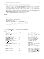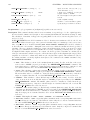
1
MODELLER A Program for Protein Structure Modeling Release 7v7 Andrej Šali with help from Ben Webb, M.S. Madhusudhan, Min-Yi Shen, Marc A. Martı-Renom, Narayanan Eswar, Frank Alber, Baldomero Oliva, András Fiser, Roberto Sánchez, Bozidar Yerkovich, Azat Badretdinov, Francisco Melo, John P. Overington, and Eric Feyfant email [email protected] URL http://salilab.org/modeller/ September 2004 ii Contents Copyright notice xiii Acknowledgments xv 1 Introduction 1 1.1 What is Modeller? . . . . . . . . . . . . . . . . . . . . . . . . . . . . . . . . . . . . . . . . . . . . . 1 1.2 Modeller bibliography . . . . . . . . . . . . . . . . . . . . . . . . . . . . . . . . . . . . . . . . . . . 2 1.3 Distribution . . . . . . . . . . . . . . . . . . . . . . . . . . . . . . . . . . . . . . . . . . . . . . . . . . 3 1.4 Installation . . . . . . . . . . . . . . . . . . . . . . . . . . . . . . . . . . . . . . . . . . . . . . . . . . 4 1.5 Bug reports . . . . . . . . . . . . . . . . . . . . . . . . . . . . . . . . . . . . . . . . . . . . . . . . . . 7 1.6 Method for comparative protein structure modeling by Modeller . . . . . . . . . . . . . . . . . . . 8 1.7 Tutorial on using Modeller for comparative modeling . . . . . . . . . . . . . . . . . . . . . . . . . 10 1.7.1 Preparing input files . . . . . . . . . . . . . . . . . . . . . . . . . . . . . . . . . . . . . . . . . 10 1.7.2 Running Modeller . . . . . . . . . . . . . . . . . . . . . . . . . . . . . . . . . . . . . . . . . 11 1.7.3 Automated alignment and comparative modeling . . . . . . . . . . . . . . . . . . . . . . . . . 11 1.8 Frequently asked questions (FAQ) and examples . . . . . . . . . . . . . . . . . . . . . . . . . . . . . 13 1.9 Modeller updates . . . . . . . . . . . . . . . . . . . . . . . . . . . . . . . . . . . . . . . . . . . . . 24 1.9.1 Changes since release 6v2 . . . . . . . . . . . . . . . . . . . . . . . . . . . . . . . . . . . . . . 24 1.9.2 Changes between releases 4 and 6v2 . . . . . . . . . . . . . . . . . . . . . . . . . . . . . . . . 24 2 Modeller commands 2.1 2.2 27 Miscellaneous rules and features of Modeller . . . . . . . . . . . . . . . . . . . . . . . . . . . . . . 27 2.1.1 Modeller system . . . . . . . . . . . . . . . . . . . . . . . . . . . . . . . . . . . . . . . . . . 27 2.1.2 Running Modeller scripts . . . . . . . . . . . . . . . . . . . . . . . . . . . . . . . . . . . . . 27 2.1.3 Controlling breakpoints and the amount of output . . . . . . . . . . . . . . . . . . . . . . . . 28 2.1.4 File naming . . . . . . . . . . . . . . . . . . . . . . . . . . . . . . . . . . . . . . . . . . . . . . 28 2.1.5 File types . . . . . . . . . . . . . . . . . . . . . . . . . . . . . . . . . . . . . . . . . . . . . . . 30 2.1.6 Format of the command description . . . . . . . . . . . . . . . . . . . . . . . . . . . . . . . . 30 Stereochemical parameters and molecular topology . . . . . . . . . . . . . . . . . . . . . . . . . . . . 32 2.2.1 Modeling residues with non-existing or incomplete entries in the topology and parameter libraries . . . . . . . . . . . . . . . . . . . . . . . . . . . . . . . . . . . . . . . . . . . . . . . . 32 2.2.2 READ RESTYP LIB — read residue type library . . . . . . . . . . . . . . . . . . . . . . . . 33 2.2.3 READ TOPOLOGY — read residue topology library . . . . . . . . . . . . . . . . . . . . . . 33 2.2.4 READ PARAMETERS — read parameters library . . . . . . . . . . . . . . . . . . . . . . . . 34 2.2.5 READ ATOM CLASSES — read classification of atom types . . . . . . . . . . . . . . . . . . 34 iii iv CONTENTS 2.2.6 GENERATE TOPOLOGY — generate MODEL topology . . . . . . . . . . . . . . . . . . . . 34 2.2.7 PATCH — patch MODEL topology . . . . . . . . . . . . . . . . . . . . . . . . . . . . . . . . 35 2.2.8 PATCH SS TEMPLATES — guess MODEL disulfides from templates . . . . . . . . . . . . . 36 2.2.9 PATCH SS MODEL — guess MODEL disulfides from model structure . . . . . . . . . . . . . 38 2.2.10 MUTATE MODEL — mutate selected MODEL residues . . . . . . . . . . . . . . . . . . . . . 38 2.2.11 MAKE TOPOLOGY MODEL — make a subset topology library . . . . . . . . . . . . . . . . 39 2.2.12 WRITE TOPOLOGY MODEL — write residue topology library . . . . . . . . . . . . . . . . 40 2.3 Handling of atomic coordinates . . . . . . . . . . . . . . . . . . . . . . . . . . . . . . . . . . . . . . . 41 2.3.1 READ MODEL — read coordinates for MODEL . . . . . . . . . . . . . . . . . . . . . . . . . 41 2.3.2 READ MODEL2 — read coordinates for MODEL2 . . . . . . . . . . . . . . . . . . . . . . . . 41 2.3.3 WRITE MODEL — write MODEL . . . . . . . . . . . . . . . . . . . . . . . . . . . . . . . . 42 2.3.4 WRITE MODEL2 — write MODEL2 . . . . . . . . . . . . . . . . . . . . . . . . . . . . . . . 42 2.3.5 BUILD MODEL — build MODEL coordinates from topology . . . . . . . . . . . . . . . . . . 43 2.3.6 UNBUILD MODEL — undefine MODEL coordinates . . . . . . . . . . . . . . . . . . . . . . 44 2.3.7 TRANSFER XYZ — copy templates’ coordinates to MODEL . . . . . . . . . . . . . . . . . . 44 2.3.8 TRANSFER RES NUMB — residue numbers from MODEL2 to MODEL . . . . . . . . . . . 46 2.3.9 RENAME SEGMENTS — rename MODEL segments . . . . . . . . . . . . . . . . . . . . . . 47 2.3.10 PICK ATOMS — select atoms in MODEL . . . . . . . . . . . . . . . . . . . . . . . . . . . . 47 2.3.11 PICK HOT ATOMS — pick atoms violating restraints . . . . . . . . . . . . . . . . . . . . . 50 2.3.12 RANDOMIZE XYZ — randomize MODEL coordinates . . . . . . . . . . . . . . . . . . . . . 51 2.3.13 IUPAC MODEL — standardize certain dihedral angles . . . . . . . . . . . . . . . . . . . . . 52 2.3.14 REORDER ATOMS — standardize order of MODEL atoms . . . . . . . . . . . . . . . . . . 52 2.3.15 ROTATE DIHEDRALS — change dihedral angles . . . . . . . . . . . . . . . . . . . . . . . . 53 2.3.16 ORIENT MODEL — center and orient MODEL . . . . . . . . . . . . . . . . . . . . . . . . . 54 2.3.17 ROTATE MODEL — rotate and translate MODEL . . . . . . . . . . . . . . . . . . . . . . . 54 2.3.18 WRITE DATA — write derivative MODEL data . . . . . . . . . . . . . . . . . . . . . . . . . 55 2.3.19 WRITE PDB XREF — write residue number/index correspondence . . . . . . . . . . . . . . 57 2.3.20 MAKE REGION — define a random surface patch of atoms . . . . . . . . . . . . . . . . . . 58 2.4 Comparison and searching of sequences and structures . . . . . . . . . . . . . . . . . . . . . . . . . . 60 2.4.1 Alignment file format . . . . . . . . . . . . . . . . . . . . . . . . . . . . . . . . . . . . . . . . 60 2.4.2 READ ALIGNMENT — read sequences and/or their alignment . . . . . . . . . . . . . . . . 62 2.4.3 READ ALIGNMENT2 — read 2nd alignment . . . . . . . . . . . . . . . . . . . . . . . . . . 63 2.4.4 CHECK ALIGNMENT — check alignment for modeling . . . . . . . . . . . . . . . . . . . . . 64 2.4.5 COLOR ALN MODEL — color MODEL according to alignment . . . . . . . . . . . . . . . . 64 2.4.6 COMPARE ALIGNMENTS — compare two alignments . . . . . . . . . . . . . . . . . . . . . 65 2.4.7 SEQUENCE TO ALI — copy MODEL sequence and coordinates to alignment . . . . . . . . 66 2.4.8 WRITE ALIGNMENT — write sequences and/or their alignment . . . . . . . . . . . . . . . 67 2.4.9 EDIT ALIGNMENT — edit overhangs in alignment . . . . . . . . . . . . . . . . . . . . . . . 68 2.4.10 DESCRIBE — describe proteins . . . . . . . . . . . . . . . . . . . . . . . . . . . . . . . . . . 69 2.4.11 ID TABLE — calculate percentage sequence identities . . . . . . . . . . . . . . . . . . . . . . 69 2.4.12 SEQUENCE COMPARISON — compare sequences in alignment . . . . . . . . . . . . . . . . 70 2.4.13 DENDROGRAM — clustering . . . . . . . . . . . . . . . . . . . . . . . . . . . . . . . . . . . 71 2.4.14 PRINCIPAL COMPONENTS — clustering . . . . . . . . . . . . . . . . . . . . . . . . . . . . 71 CONTENTS v 2.4.15 ALIGN — align two (blocks of) sequences . . . . . . . . . . . . . . . . . . . . . . . . . . . . . 71 2.4.16 ALIGN2D — align sequences with structures . . . . . . . . . . . . . . . . . . . . . . . . . . . 73 2.4.17 MALIGN — align two or more sequences . . . . . . . . . . . . . . . . . . . . . . . . . . . . . 75 2.4.18 ALIGN CONSENSUS — consensus sequence alignment . . . . . . . . . . . . . . . . . . . . . 76 2.4.19 SUPERPOSE — superpose MODEL2 on MODEL given alignment . . . . . . . . . . . . . . . 77 2.4.20 COMPARE — compare 3D structures given alignment . . . . . . . . . . . . . . . . . . . . . . 80 2.4.21 ALIGN3D — align two structures . . . . . . . . . . . . . . . . . . . . . . . . . . . . . . . . . 81 2.4.22 MALIGN3D — align two or more structures . . . . . . . . . . . . . . . . . . . . . . . . . . . 82 2.4.23 ALN TO PROF — convert alignment to profile format . . . . . . . . . . . . . . . . . . . . . 84 2.4.24 PROF TO ALN — profile to alignment . . . . . . . . . . . . . . . . . . . . . . . . . . . . . . 85 2.4.25 READ PROFILE — read a profile of a sequence . . . . . . . . . . . . . . . . . . . . . . . . . 85 2.4.26 WRITE PROFILE — write a profile . . . . . . . . . . . . . . . . . . . . . . . . . . . . . . . . 87 2.4.27 BUILD PROFILE — Build a profile for a given sequence or alignment . . . . . . . . . . . . . 87 2.4.28 READ SEQUENCE DB — read a database of sequences . . . . . . . . . . . . . . . . . . . . 90 2.4.29 WRITE SEQUENCE DB — write a database of sequences . . . . . . . . . . . . . . . . . . . 90 2.4.30 EXPAND ALIGNMENT — put all models into alignment . . . . . . . . . . . . . . . . . . . . 91 2.4.31 SEQUENCE SEARCH — search for similar sequences . . . . . . . . . . . . . . . . . . . . . . 91 2.4.32 SEQFILTER — cluster sequences by sequence-identity . . . . . . . . . . . . . . . . . . . . . . 93 2.4.33 DELETE ALIGNMENT — delete alignment . . . . . . . . . . . . . . . . . . . . . . . . . . . 95 2.4.34 SEGMENT MATCHING — align segments . . . . . . . . . . . . . . . . . . . . . . . . . . . . 95 2.5 Calculation of spatial restraints . . . . . . . . . . . . . . . . . . . . . . . . . . . . . . . . . . . . . . . 97 2.5.1 Specification of restraints . . . . . . . . . . . . . . . . . . . . . . . . . . . . . . . . . . . . . . 97 2.5.2 Specification of pseudo atoms . . . . . . . . . . . . . . . . . . . . . . . . . . . . . . . . . . . . 98 2.5.3 MAKE RESTRAINTS — make restraints . . . . . . . . . . . . . . . . . . . . . . . . . . . . . 103 2.5.4 DEFINE SYMMETRY — define similar segments . . . . . . . . . . . . . . . . . . . . . . . . 107 2.5.5 PICK RESTRAINTS — pick restraints for selected atoms . . . . . . . . . . . . . . . . . . . . 109 2.5.6 CONDENSE RESTRAINTS — remove unselected restraints . . . . . . . . . . . . . . . . . . 110 2.5.7 ADD RESTRAINT — add restraint . . . . . . . . . . . . . . . . . . . . . . . . . . . . . . . . 111 2.5.8 DELETE RESTRAINT — unselect restraint . . . . . . . . . . . . . . . . . . . . . . . . . . . 112 2.5.9 REINDEX RESTRAINTS — renumber MODEL2 restraints for MODEL . . . . . . . . . . . 112 2.5.10 SPLINE RESTRAINTS — approximate restraints by splines . . . . . . . . . . . . . . . . . . 113 2.5.11 READ RESTRAINTS — read spatial restraints . . . . . . . . . . . . . . . . . . . . . . . . . 114 2.5.12 WRITE RESTRAINTS — write spatial restraints . . . . . . . . . . . . . . . . . . . . . . . . 114 2.6 Optimization of the model . . . . . . . . . . . . . . . . . . . . . . . . . . . . . . . . . . . . . . . . . . 115 2.6.1 MAKE SCHEDULE — create optimization schedule . . . . . . . . . . . . . . . . . . . . . . . 115 2.6.2 READ SCHEDULE — read optimization schedule . . . . . . . . . . . . . . . . . . . . . . . . 116 2.6.3 WRITE SCHEDULE — write optimization schedule . . . . . . . . . . . . . . . . . . . . . . . 116 2.6.4 ENERGY — evaluate MODEL given restraints . . . . . . . . . . . . . . . . . . . . . . . . . . 117 2.6.5 OPTIMIZE — optimize MODEL given restraints 2.6.6 SWITCH TRACE — open new optimization trace file . . . . . . . . . . . . . . . . . . . . . . 124 2.6.7 DEBUG FUNCTION — test code self-consistency . . . . . . . . . . . . . . . . . . . . . . . . 124 3 Modeller scripts 3.1 . . . . . . . . . . . . . . . . . . . . . . . . 120 127 Flowchart of comparative modeling by Modeller . . . . . . . . . . . . . . . . . . . . . . . . . . . . 127 vi CONTENTS 3.2 Script for comparative modeling . . . . . . . . . . . . . . . . . . . . . . . . . . . . . . . . . . . . . . 129 3.3 Script for modeling of loops . . . . . . . . . . . . . . . . . . . . . . . . . . . . . . . . . . . . . . . . . 132 4 Top, Modeller scripting language 135 4.1 The source file . . . . . . . . . . . . . . . . . . . . . . . . . . . . . . . . . . . . . . . . . . . . . . . . 135 4.2 Top Commands . . . . . . . . . . . . . . . . . . . . . . . . . . . . . . . . . . . . . . . . . . . . . . . 136 4.2.1 DEFINE INTEGER — define integer variables . . . . . . . . . . . . . . . . . . . . . . . . . . 137 4.2.2 DEFINE LOGICAL — define logical variables . . . . . . . . . . . . . . . . . . . . . . . . . . 137 4.2.3 DEFINE REAL — define real variables . . . . . . . . . . . . . . . . . . . . . . . . . . . . . . 137 4.2.4 DEFINE STRING — define string variables . . . . . . . . . . . . . . . . . . . . . . . . . . . . 137 4.2.5 SET — set variable . . . . . . . . . . . . . . . . . . . . . . . . . . . . . . . . . . . . . . . . . 137 4.2.6 OPERATE — perform mathematic operation . . . . . . . . . . . . . . . . . . . . . . . . . . . 138 4.2.7 STRING OPERATE — perform string operation . . . . . . . . . . . . . . . . . . . . . . . . . 138 4.2.8 RESET — reset Top . . . . . . . . . . . . . . . . . . . . . . . . . . . . . . . . . . . . . . . . 138 4.2.9 OPEN — open input file . . . . . . . . . . . . . . . . . . . . . . . . . . . . . . . . . . . . . . 138 4.2.10 TIME MARK — print current date, time, and CPU time . . . . . . . . . . . . . . . . . . . . 139 4.2.11 WRITE — write Top objects . . . . . . . . . . . . . . . . . . . . . . . . . . . . . . . . . . . . 139 4.2.12 READ — read record from input file . . . . . . . . . . . . . . . . . . . . . . . . . . . . . . . . 139 4.2.13 CLOSE — close an input file . . . . . . . . . . . . . . . . . . . . . . . . . . . . . . . . . . . . 139 4.2.14 DELETE FILE — delete a file . . . . . . . . . . . . . . . . . . . . . . . . . . . . . . . . . . . 140 4.2.15 WRITE TOP — write the Top program . . . . . . . . . . . . . . . . . . . . . . . . . . . . . 140 4.2.16 SYSTEM — execute system command . . . . . . . . . . . . . . . . . . . . . . . . . . . . . . . 140 4.2.17 INQUIRE — check if file exists . . . . . . . . . . . . . . . . . . . . . . . . . . . . . . . . . . . 140 4.2.18 GO TO — jump to label . . . . . . . . . . . . . . . . . . . . . . . . . . . . . . . . . . . . . . 140 4.2.19 LABEL — place jump label . . . . . . . . . . . . . . . . . . . . . . . . . . . . . . . . . . . . . 140 4.2.20 INCLUDE — include Top file . . . . . . . . . . . . . . . . . . . . . . . . . . . . . . . . . . . 141 4.2.21 CALL — call Top subroutine . . . . . . . . . . . . . . . . . . . . . . . . . . . . . . . . . . . . 141 4.2.22 SUBROUTINE — define Top subroutine . . . . . . . . . . . . . . . . . . . . . . . . . . . . . 141 4.2.23 RETURN — return from Top subroutine . . . . . . . . . . . . . . . . . . . . . . . . . . . . . 141 4.2.24 END SUBROUTINE — end definition of Top subroutine . . . . . . . . . . . . . . . . . . . . 141 4.2.25 DO — DO loop . . . . . . . . . . . . . . . . . . . . . . . . . . . . . . . . . . . . . . . . . . . . 141 4.2.26 IF — conditional statement for numbers . . . . . . . . . . . . . . . . . . . . . . . . . . . . . . 141 4.2.27 STRING IF — conditional statement for strings . . . . . . . . . . . . . . . . . . . . . . . . . 142 4.2.28 STOP — exit Top . . . . . . . . . . . . . . . . . . . . . . . . . . . . . . . . . . . . . . . . . . 142 4.3 Predefined Top variables . . . . . . . . . . . . . . . . . . . . . . . . . . . . . . . . . . . . . . . . . . 142 5 Methods 5.1 5.2 145 Dynamic programming for sequence and structure comparison and searching . . . . . . . . . . . . . 145 5.1.1 Pairwise comparison . . . . . . . . . . . . . . . . . . . . . . . . . . . . . . . . . . . . . . . . . 145 5.1.2 Variable gap penalty . . . . . . . . . . . . . . . . . . . . . . . . . . . . . . . . . . . . . . . . . 146 5.1.3 Local versus global alignment . . . . . . . . . . . . . . . . . . . . . . . . . . . . . . . . . . . . 146 5.1.4 Similarity versus distance scores . . . . . . . . . . . . . . . . . . . . . . . . . . . . . . . . . . 147 5.1.5 Multiple comparisons . . . . . . . . . . . . . . . . . . . . . . . . . . . . . . . . . . . . . . . . 147 Optimization of the objective function by Modeller . . . . . . . . . . . . . . . . . . . . . . . . . . 147 CONTENTS vii 5.2.1 Function . . . . . . . . . . . . . . . . . . . . . . . . . . . . . . . . . . . . . . . . . . . . . . . . 147 5.2.2 Optimizers . . . . . . . . . . . . . . . . . . . . . . . . . . . . . . . . . . . . . . . . . . . . . . 148 5.3 5.4 Equations used in the derivation of the molecular pdf . . . . . . . . . . . . . . . . . . . . . . . . . . 149 5.3.1 Features and their derivatives . . . . . . . . . . . . . . . . . . . . . . . . . . . . . . . . . . . . 149 5.3.2 Restraints and their derivatives . . . . . . . . . . . . . . . . . . . . . . . . . . . . . . . . . . . 151 List of commands, arguments, and default values . . . . . . . . . . . . . . . . . . . . . . . . . . . . . 155 viii CONTENTS List of Figures 1.1 Comparative protein modeling by satisfaction of spatial restraints. . . . . . . . . . . . . . . . . . . . . 8 1.2 Sample spatial restraint. . . . . . . . . . . . . . . . . . . . . . . . . . . . . . . . . . . . . . . . . . . . 9 1.3 Optimization of the objective function. . . . . . . . . . . . . . . . . . . . . . . . . . . . . . . . . . . . 9 ix x LIST OF FIGURES List of Tables 2.1 List of file types. . . . . . . . . . . . . . . . . . . . . . . . . . . . . . . . . . . . . . . . . . . . . . . . 31 2.2 List of mathematical forms of restraints. . . . . . . . . . . . . . . . . . . . . . . . . . . . . . . . . . . 100 2.3 List of feature types that can be restrained. . . . . . . . . . . . . . . . . . . . . . . . . . . . . . . . . . 101 2.4 List of “physical” restraint types. . . . . . . . . . . . . . . . . . . . . . . . . . . . . . . . . . . . . . . 102 2.5 Columns in an optimization trace file. . . . . . . . . . . . . . . . . . . . . . . . . . . . . . . . . . . . 124 3.1 List of Modeller scripts. . . . . . . . . . . . . . . . . . . . . . . . . . . . . . . . . . . . . . . . . . . 127 4.1 List of variable types in Top. . . . . . . . . . . . . . . . . . . . . . . . . . . . . . . . . . . . . . . . . 136 4.2 Predefined Top variables . . . . . . . . . . . . . . . . . . . . . . . . . . . . . . . . . . . . . . . . . . . 143 xi xii LIST OF TABLES Copyright notice Modeller, a protein structure modeling program. c 1989–2004 Andrej Šali. Copyright This program is distributed in the hope that it will be useful, but without any warranty; without even the implied warranty of merchantability or fitness for any purpose. The entire risk as to the quality and performance of the program is with the user. Distribution of the program is allowed only with the author’s written consent. xiii xiv LIST OF TABLES Acknowledgments I am grateful to my PhD supervisor Professor Tom L. Blundell in whose laboratory at Birkbeck College the program was initiated. I would also like to thank Professor Martin Karplus who allowed some of the data in the Charmm topology and library files to be used with Modeller. I am in debt to the Modeller users for their constructive criticisms and suggestions. Modeller was written when at 1989–1990: Department of Crystallography, Birkbeck College University of London, Malet St, London WC1E 7HX, UK. 1990–1991: ICRF Unit of Structural Molecular Biology, Birkbeck College Malet St, London WC1E 7HX, UK. 1991–1994: Department of Chemistry, Harvard University 12 Oxford St, Cambridge, MA 02138, USA. 1995–2003: The Rockefeller University, 1230 York Ave, New York, NY 10021, USA. 2003–: University of California, San Francisco, 600 16th Street, San Francisco, CA 94143, USA. xv xvi LIST OF TABLES Chapter 1 Introduction 1.1 What is Modeller? Modeller is a computer program that models three-dimensional structures of proteins and their assemblies by satisfaction of spatial restraints. Modeller is most frequently used for homology or comparative protein structure modeling: The user provides an alignment of a sequence to be modeled with known related structures and Modeller will automatically calculate a model with all non-hydrogen atoms. More generally, the input to the program are restraints on the spatial structure of the amino acid sequence(s) and ligands to be modeled. The output is a 3D structure that satisfies these restraints as well as possible. Restraints can in principle be derived from a number of different sources. These include related protein structures (comparative modeling), NMR experiments (NMR refinement), rules of secondary structure packing (combinatorial modeling), cross-linking experiments, fluorescence spectroscopy, image reconstruction in electron microscopy, site-directed mutagenesis, intuition, residue–residue and atom–atom potentials of mean force, etc. The restraints can operate on distances, angles, dihedral angles, pairs of dihedral angles and some other spatial features defined by atoms or pseudo atoms. Presently, Modeller automatically derives the restraints only from the known related structures and their alignment with the target sequence. A 3D model is obtained by optimization of a molecular probability density function (pdf). The molecular pdf for comparative modeling is optimized with the variable target function procedure in Cartesian space that employs methods of conjugate gradients and molecular dynamics with simulated annealing. Modeller can also perform multiple comparison of protein sequences and/or structures, clustering of proteins, and searching of sequence databases. The program is used with a scripting language and does not include any graphics. It is written in standard Fortran 90 and is meant to run on a Unix or Windows computer. 1 2 CHAPTER 1. INTRODUCTION 1.2 Modeller bibliography In your publications using Modeller, please quote A. Šali and T. L. Blundell. Comparative protein modelling by satisfaction of spatial restraints. J. Mol. Biol. 234, 779–815, 1993. More information about the methods implemented in Modeller, their use, applications, and limitations can be found in the papers listed on our web site at http://salilab.org/publications/. Here is a subset of these publications: 1. A. Šali and T. L. Blundell. Comparative protein modelling by satisfaction of spatial restraints. J. Mol. Biol. 234, 779–815, 1993. 2. A. Šali, A. and J. P. Overington. Derivation of rules for comparative protein modeling from a database of protein structure alignments. Protein Science 3, 1582–1596, 1994. 3. R. Sánchez and A. Šali. Comparative protein structure modeling: Introduction and practical examples with Modeller. In Protein Structure Prediction: Methods and Protocols, D.M. Webster, editor, 97–129. Humana Press, 2000. 4. M. A. Martı́-Renom, A. Stuart, A. Fiser, R. Sánchez, F. Melo and A. Šali. Comparative protein structure modeling of genes and genomes. Ann. Rev. Biophys. Biomolec. Struct. 29, 291–325, 2000. 5. A. Fiser, R. K. G. Do and A. Šali. Modeling of loops in protein structures. Protein Science 9, 1753–1773, 2000. 6. F. Melo, R. Sánchez, A. Sali. Statistical potentials for fold assessment. Protein Science 11, 430–448, 2002. 7. M. A. Martı́-Renom, B. Yerkovich, and A. Sali. Comparative protein structure prediction. John Wiley & Sons, Inc. Current Protocols in Protein Science 1, 2.9.1 – 2.9.22, 2002. 8. U. Pieper, N. Eswar, A. C. Stuart, V. A. Ilyin and A. Sali. MODBASE, a database of annotated comparative protein structure models. Nucleic Acids Research 30, 255–259, 2002. 9. A. Fiser and A. Sali. MODELLER: generation and refinement of homology models. In Methods in Enzymology, C.W. Carter and R.M. Sweet, eds. Academic Press, San Diego, in press. 10. N. Eswar, B. John, N. Mirkovic, A. Fiser, V. A. Ilyin, U. Pieper, A. C. Stuart, M. A. Martı́-Renom, M. S. Madhusudhan, B. Yerkovich and A. Sali. Tools for comparative protein structure modeling and analysis, submitted. 1.3. DISTRIBUTION 1.3 3 Distribution Modeller is available free of charge to academic non-profit institutions. First, please download the Modeller distribution file from the Modeller home page at http://salilab.org/modeller/. Next, please obtain the Modeller key from the academic license server, also accessible from the Modeller home page. This key is required to run Modeller, and you should provide it to the Windows or Unix install program when prompted to do so. (If installing manually, the key needs to be assigned to the environment variable KEY MODELLER7v7 in your login or Modeller startup script.) See file INSTALLATION for further installation instructions. There is a Modeller users email list. You can access it from the Modeller home page or subscribe to it directly by sending an email message with the word “subscribe” in its body to modeller [email protected]. A graphical interface to Modeller is available as part of Quanta, InsightII, and Discovery Studio, interactive molecular modeling programs from Accelrys Inc., San Diego, with many tools for protein modeling and structural analysis. These programs facilitate preparation of input files for Modeller (e.g., an alignment file) as well as an analysis of results (e.g., an evaluation of the models). If you are interested in these programs, please contact Dr. Dana Haley-Vicente Accelrys Inc. 9685 Scranton Road San Diego, CA 92121-3752, USA tel +1-858-799-5322; fax +1-858-799-5100 email [email protected]; URL http://www.accelrys.com/ 4 CHAPTER 1. INTRODUCTION 1.4 Installation The following installation instructions are from the INSTALLATION file in the root directory of the Modeller distribution. See Section 1.3 for how to obtain Modeller. INSTALLATION M O D E L L E R 7v7 Copyright(c) 1989-2004 Andrej Sali All Rights Reserved ** PLATFORMS MODELLER is written in Fortran 90 and runs on Pentium PC’s (Linux and Windows XP), Apple Macintosh (OS X 10.2), Linux Itanium 2 systems, and workstations from Silicon Graphics (IRIX), Sun (Solaris), IBM (AIX), and DEC Alpha (OSF/1). ** INSTALLATION See file README for information about how to get MODELLER. The source code is not generally available. Hence, most users are limited to the compiled versions of MODELLER. The program is distributed as a single install file that contains scripts, libraries, examples, documentation (in PDF and HTML formats) and executables for the supported platforms and operating systems. Please refer to the relevant section below for your platform: ** WINDOWS INSTALLATION 1) If using Windows NT/2000/XP, log on as a Computer Administrator. (For older systems, e.g. Windows 98, just log on as normal.) 2) Download the Windows installer modeller7v7.exe and save it to your Desktop. 3) Double-click on the modeller7v7 file to start the installer. 4) Tell the installer where to install Modeller, and enter your Modeller license key when prompted. 5) Once the install is complete, use the Modeller link from the Start Menu to start a Command Prompt from where you can run Modeller scripts. You can then delete the original installer file from your Desktop. 6) Examples can be found in the ’examples’ subdirectory. Note, however, that if you use NT/2000/XP, and are NOT an Administrator user, you will need to make a copy of this directory elsewhere, as Windows 1.4. INSTALLATION 5 will not allow Modeller to write output files into this directory. ** MAC OS X INSTALLATION 1) Download the Modeller.dmg file to your Desktop. 2) Double-click on the Modeller.dmg file to open the disk image. 3) Double-click on the Install.command file within this image. Tell the installer where to install Modeller, and enter your Modeller license key when prompted. 4) Once the install is complete, you can run the Modeller script from a Terminal window. You can then drag both the ’Modeller 7v7’ disk image and the Modeller.dmg file to your trash. ** LINUX INSTALLATION (USING RPM) 1) Download the modeller-7v7-1.i386.rpm file. 2) Install the RPM file with the following command, replacing XXXX with your Modeller license key: env KEY_MODELLER7v7=XXXX rpm -ivh modeller-7v7-1.i386.rpm 3) Documentation and examples can be found in the /usr/lib/modeller7v7/ directory. Note that if you are not root, you will need to make a copy of the examples directory in order to run them. ** GENERIC UNIX INSTALLATION 1) Download the modeller7v7.tar.gz file into a temporary directory on your computer. 2) Open a console or terminal (e.g. xterm, Konsole, GNOME terminal) and change to the directory where you downloaded the .tar.gz file. Unpack the file with the following commands: gunzip modeller7v7.tar.gz tar -xvf modeller7v7.tar The result of unpacking will be the directory ./modeller7v7, containing the following uncompressed files and directories: doc/ examples/ Install INSTALLATION README modlib/ bin/ MODELLER documentation directory directory containing examples and tutorials installation script this file file describing distribution and registration libraries and data files for the program .top script files and MODELLER executables 6 CHAPTER 1. INTRODUCTION 3) Go to the ./modeller7v7 directory and run the installation script: ./Install Answer several questions as prompted. If you make a mistake, you can re-run the script. For additional information visit our web site: http://salilab.org/modeller/ Sincerely, MODELLER Team September 2004 1.5. BUG REPORTS 1.5 7 Bug reports Please report Modeller bugs by e-mail to the Modeller users list at modeller [email protected]. It is best if you attach all of your input and output files to your e-mail. 8 CHAPTER 1. INTRODUCTION 1.6 Method for comparative protein structure modeling by Modeller Modeller implements an automated approach to comparative protein structure modeling by satisfaction of spatial restraints (Figure 1.1) [Šali & Blundell, 1993]. The method and its applications to biological problems are described in detail in references listed in Section 1.2. Briefly, the core modeling procedure begins with an alignment of the sequence to be modeled (target) with related known 3D structures (templates). This alignment is usually the input to the program. The output is a 3D model for the target sequence containing all mainchain and sidechain nonhydrogen atoms. Given an alignment, the model is obtained without any user intervention. First, many distance and dihedral angle restraints on the target sequence are calculated from its alignment with template 3D structures (Figure 1.2). The form of these restraints was obtained from a statistical analysis of the relationships between many pairs of homologous structures. This analysis relied on a database of 105 family alignments that included 416 proteins with known 3D structure [Šali & Overington, 1994]. By scanning the database, tables quantifying various correlations were obtained, such as the correlations between two equivalent C α – Cα distances, or between equivalent mainchain dihedral angles from two related proteins. These relationships were expressed as conditional probability density functions (pdf’s) and can be used directly as spatial restraints. For example, probabilities for different values of the mainchain dihedral angles are calculated from the type of a residue considered, from mainchain conformation of an equivalent residue, and from sequence similarity between the two proteins. Another example is the pdf for a certain Cα –Cα distance given equivalent distances in two related protein structures (Figure 1.2). An important feature of the method is that the spatial restraints are obtained empirically, from a database of protein structure alignments. Next, the spatial restraints and Charmm energy terms enforcing proper stereochemistry [MacKerell et al., 1998] are combined into an objective function. Finally, the model is obtained by optimizing the objective function in Cartesian space. The optimization is carried out by the use of the variable target function method [Braun & Gõ, 1985] employing methods of conjugate gradients and molecular dynamics with simulated annealing (Figure 1.3). Several slightly different models can be calculated by varying the initial structure. The variability among these models can be used to estimate the errors in the corresponding regions of the fold. There are additional specialized modeling protocols, such as that for the modeling of loops (Section 3.3). 3D GRISFFEDAGF-GHCYECSSDC-NLQP 3D GKITFYEDRGFQGHCYECSSDC-NLQP SEQ GKITFYEDRG---RCYECSSDCPNLQP FY E RC IT D R G P NLQ G K DC 2. EXTRACT SPATIAL RESTRAINTS: CS S YE 1. ALIGN SEQUENCE WITH STRUCTURES: P 3. SATISFY SPATIAL RESTRAINTS: Figure 1.1: Comparative protein modeling by satisfaction of spatial restraints. First, the known, template 3D structures (‘3D’) are aligned with the target sequence to be modeled (‘SEQ’) Second, spatial features, such as C α –Cα distances, hydrogen bonds, and mainchain and sidechain dihedral angles, are transferred from the templates to the target. Thus, a number of spatial restraints on its structure are obtained. Third, the 3D model is obtained by satisfying all the restraints as well as possible. 1.6. METHOD FOR COMPARATIVE PROTEIN STRUCTURE MODELING BY MODELLER 9 FREQUENCY 4E6 3E6 2E6 1E6 0 15 17 19 21 23 Cα − Cα DISTANCE 25 [Å] Figure 1.2: Sample spatial restraint. A restraint on a given Cα –Cα distance, d, is expressed as a conditional probability OBJECTIVE FUNCTION density function that depends on two other equivalent distances (d0 = 17.0 and d00 = 23.5): p(d/d0 , d00 ). The restraint (continuous line) is obtained by least-squares fitting a sum of two Gaussian functions to the histogram, which in turn is derived from the database of alignments of protein structures. In practice, more complicated restraints are used that depend on additional information, such as similarity between the proteins, solvent accessibility, and distance from a gap in the alignment [Šali & Blundell, 1993]. 0 340 770 1190 1660 1810 6750 8000 6000 4000 2000 0 0 1000 2000 3000 4000 ITERATION 5000 6000 7000 Figure 1.3: Optimization of the objective function. Optimization of the objective function (curve) starts with a distorted average of template structures (not with an extended structure as shown here). The iteration number is indicated below each sample structure. In this run, the first ∼ 2, 000 iterations correspond to the variable target function method relying on the conjugate gradients technique. This approach first satisfies sequentially local restraints and slowly introduces longer range restraints until the complete objective function is optimized. In the last 4,750 iterations for this model, molecular dynamics with simulated annealing is used to refine the model. Typically, a model is calculated in the order of minutes on a PC workstation. 10 1.7 CHAPTER 1. INTRODUCTION Tutorial on using Modeller for comparative modeling Simple demonstrations of Modeller in all steps of comparative protein structure modeling, including fold assignment, sequence-structure alignment, model building, and model assessment, can be found in references listed at http://salilab.org/modeller/user manual.shtml. A number of additional tools useful in comparative modeling are listed at http://salilab.org/bioinformatics resources.shtml. Specifically, users have access to ModBase, a comprehensive database of comparative models for all known protein sequences detectably related to at least one known protein structure; ModWeb, a web server for automated comparative protein structure modeling; and ModLoop, a web server for automated modeling of loops in protein structures. For “frequentlyasked-questions” (FAQ), see Section 1.8. The rest of this section is a ‘hands on’ description of the most basic use of Modeller in comparative modeling, in which the input are Protein Data Bank (PDB) atom files of known protein structures, their alignment with the target sequence to be modeled, and the output is a model for the target that includes all non-hydrogen atoms. Although Modeller can find template structures as well as calculate sequence and structure alignments, it is better in the difficult cases to identify the templates and prepare the alignment carefully by other means. The alignment can also contain very short segments such as loops, secondary structure motifs, etc. This tutorial assumes that Modeller is already installed on your computer and that appropriate changes have been made to your login script to install you as a Modeller user. See Section 1.4 for more details on installation (also in the INSTALLATION file in the Modeller distribution directory). 1.7.1 Preparing input files The sample input files in this tutorial can be found in the examples/tutorial-model directory of the Modeller distribution. There are three kinds of input files: Protein Data Bank atom files with coordinates for the template structures, the alignment file with the alignment of the template structures with the target sequence, and Modeller commands in a script file that instruct Modeller what to do. Atom files Each atom file is named code.atm where code is a short protein code, preferably the PDB code; for example, Peptococcus aerogenes ferredoxin would be in a file 1fdx.atm. If you wish, you can also use file extensions .pdb and .ent instead of .atm. The code must be used as that protein’s identifier throughout the modeling. The atom sets do not have to be superposed by the user before comparative modeling is done. Alignment file One of the formats for the alignment file is related to the PIR database format; this is the preferred format for comparative modeling: C; A sample alignment in the PIR format; used in tutorial >P1;5fd1 structureX:5fd1:1 : :106 : :ferredoxin:Azotobacter vinelandii: 1.90: 0.19 AFVVTDNCIKCKYTDCVEVCPVDCFYEGPNFLVIHPDECIDCALCEPECPAQAIFSEDEVPEDMQEFIQLNAELA EVWPNITEKKDPLPDAEDWDGVKGKLQHLER* >P1;1fdx sequence:1fdx:1 : :54 : :ferredoxin:Peptococcus aerogenes: 2.00:-1.00 AYVINDSC--IACGACKPECPVNIIQGS--IYAIDADSCIDCGSCASVCPVGAPNPED-----------------------------------------------* See Section 2.4.1 for a detailed description of the alignment file format. Influence of the alignment on the quality of the model cannot be overemphasized. To obtain the best possible model, it is important to understand how the alignment is used by Modeller [Šali & Blundell, 1993]. In outline, for the aligned regions, Modeller tries to derive a 3D model for the target sequence that is as close to one or the other of the template structures as 1.7. TUTORIAL ON USING MODELLER FOR COMPARATIVE MODELING 11 possible while also satisfying stereochemical restraints (e.g., bond lengths, angles, non-bonded atom contacts, . . . ); the inserted regions, which do not have any equivalent segments in any of the templates, are modeled in the context of the whole molecule, but using their sequence alone. This way of deriving a model means that whenever a user aligns a target residue with a template residue, he tells Modeller to treat the aligned residues as structurally equivalent. Command CHECK ALIGNMENT can be used to find some trivial alignment mistakes. Script file The script file contains commands for Modeller, in the Top language (Chapter 4). A sample script file model-default.top to produce one model of sequence 1fdx from the known structure of 5fd1 and from the alignment between the two sequences is # Homology modelling by the MODELLER TOP routine ’model’. INCLUDE # Include the predefined TOP routines SET SET SET SET SET SET SET OUTPUT_CONTROL = 1 1 1 1 1 # uncomment to produce a large log file ALNFILE = ’alignment.ali’ # alignment filename KNOWNS = ’5fd1’ # codes of the templates SEQUENCE = ’1fdx’ # code of the target ATOM_FILES_DIRECTORY = ’./:../atom_files’ # directories for input atom files STARTING_MODEL= 1 # index of the first model ENDING_MODEL = 1 # index of the last model # (determines how many models to calculate) CALL ROUTINE = ’model’ # do homology modelling See Section 3.2 for information about the model script and its arguments. 1.7.2 Running Modeller To run Modeller with the script file model-default.top, execute the following command at your command-line prompt (e.g. a Unix console or xterm, the Mac Terminal application, or a Windows Command Prompt) mod7v7 model-default A number of intermediary files are created as the program proceeds. After about 30 seconds on a Pentium IV workstation, the final 1fdx model is written to file 1fdx.B99990001.pdb. Examine the model-default.log file for information about the run. In particular, one should always check the output of the CHECK ALIGNMENT command, which you can find by searching for ‘chkaln’. Also, check for warning and error messages by searching for ‘W>’ and ‘E>’, respectively. There should be no error messages; most often, there are some warning messages that can usually be ignored. 1.7.3 Automated alignment and comparative modeling Automated alignment and comparative modeling requires only the target sequence and the coordinates of the templates. The structural alignment of the known 3D structures and their alignment with the target sequence are derived automatically. However, the single most important factor that determines the quality of a model is the quality of the alignment. If the alignment is incorrect, the model will also be incorrect. For this reason, automated alignment for comparative modeling should not be used unless the sequences are so similar that the calculated alignment is likely to be correct, which usually requires more than 50% sequence identity. Instead, the alignment should be carefully inspected, optimized by hand, and checked by the CHECK ALIGNMENT command before used in modeling. Moreover, several iterations of alignment and modeling may be necessary in general. The sample input files for automated alignment and comparative modeling are located in directory examples/align-model-steps. The sample Top file is # A sample TOP file for fully automated comparative modeling 12 INCLUDE SET ATOM_FILES_DIRECTORY = ’./:../atom_files’ SET SEGFILE = ’alignment.seg’ SET KNOWNS = ’5fd1’ ’1fdn’ ’1fxd’ ’2fxb’ SET SEQUENCE = ’1fdx’ SET OUTPUT_CONTROL = 1 1 1 1 2 CALL ROUTINE = ’full_homol’ CHAPTER 1. INTRODUCTION # # # # # include MODELLER routines directory with input atom files input file w/ templates and target templates’ PDB codes target code # get alignment and a model The alignment.seg file is >P1;1fdx structureX:1fdx:FIRST:@:54:@:ferredoxin:Peptococcus aerogenes: 2.00:-1.00 AYVINDSCIACGACKPECPVNIIQGSIYAIDADSCIDCGSCASVCPVGAPNPED* >P1;1fdn structureX:1fdn:FIRST:@:55:@:ferredoxin:Clostrodium acidiurici: 1.84:-1.0 * >P1;5fd1 structureX:5fd1:FIRST:@:60:@:ferredoxin:Azotobacter vinelandii: 1.90:0.192 * >P1;1fxd structureX:1fxd:FIRST:@:58:@:ferredoxin:Desolfovibrio gigas: 1.70:-1.0 * >P1;2fxb structureX:2fxb:FIRST:@:60:@:ferredoxin:Bacillus thermoproteolyticus: 2.30:-1.0 * 1.8. FREQUENTLY ASKED QUESTIONS (FAQ) AND EXAMPLES 1.8 13 Frequently asked questions (FAQ) and examples Please also check the archive of the Users Mail List at http://salilab.org/archives/modeller usage/. 1. I do not care about the details of a model, I only want to calculate it very fast to get a quick idea about how it looks or to confirm that my alignment is clearly unreasonable in the structural sense. Only one model can be calculated by this routine because the starting structure is not randomized before optimization. Only a very limited amount of the variable target function optimization with conjugate gradients is done. This is usually for a factor of 3 faster than the default procedure. For example, it takes about 17 seconds of CPU time to model a 60-residue protein on an SGI workstation with a R10000-195 processor. # Very fast homology modelling by the MODELLER TOP routine ’model’. INCLUDE SET SET SET SET SET SET # Include the predefined TOP routines ALNFILE = ’alignment.ali’ # alignment filename KNOWNS = ’5fd1’ # codes of the templates SEQUENCE = ’1fdx’ # code of the target ATOM_FILES_DIRECTORY = ’./:../atom_files’ # directories for input atom files STARTING_MODEL = 2 ENDING_MODEL = 2 SET OUTPUT_CONTROL = 1 1 1 1 1 # SET OUTPUT = ’LONG’ SET FINAL_MALIGN3D = 1 CALL ROUTINE = ’very_fast’ # prepare for extremely fast optimization CALL ROUTINE = ’model’ # do homology modelling 2. How can I refine the model in successive steps? There is a pre-defined routine ’select atoms’ which selects the atoms to be moved during optimization. By default, the routine selects all atoms, but you can redefine it to select any subset of atoms and then only those atoms will be refined. They will “feel” the presence of other atoms via all the static and possibly dynamic restraints that include both selected and un-selected atoms. For example, the script below would refine only atoms in residues 1 and 2 (file ’examples/tutorial-model/model-segment.top’). The difference between this script and the one for loop modeling is that here the selected regions are optimized with the default optimization protocol and the default restraints, which generally include template-derived restraints. In contrast, the loop modeling routine does not use template-dependent restraints, but does a much more thorough optimization. # Homology modelling by the MODELLER TOP routine ’model’. # Demonstrates how to refine only a part of the model. # # You may want to use the more exhaustive "loop" modeling routines instead. # INCLUDE SET OUTPUT_CONTROL = 1 1 1 1 0 SET SET SET SET SET # Include the predefined TOP routines ALNFILE = ’alignment.ali’ # alignment filename KNOWNS = ’5fd1’ # codes of the templates SEQUENCE = ’1fdx’ # code of the target ATOM_FILES_DIRECTORY = ’./:../atom_files’ # directories for input atom files STARTING_MODEL= 3 # index of the first model 14 CHAPTER 1. INTRODUCTION SET ENDING_MODEL = 3 SET NONBONDED_SEL_ATOMS = 2 # index of the last model # (determines how many models to calculate) # selected atoms do not feel the neighbourhood CALL ROUTINE = ’model’ # do homology modelling SUBROUTINE ROUTINE = ’select_atoms’ PICK_ATOMS SELECTION_SEGMENT=’1:’ ’2:’, SELECTION_SEARCH=’segment’, ; PICK_ATOMS_SET=1, RES_TYPES=’all’, ATOM_TYPES=’all’, ; SELECTION_FROM=’all’, SELECTION_STATUS=’initialize’ RETURN END_SUBROUTINE 3. I want to model one or more loops very thoroughly (meaning spending a lot of CPU time, not necessarily modeling more accurately). Note that loops and insertions are already modeled by the default modeling routine, so you do not have to do anything special to get a model for the insertions. However, if you really want to focus on loops, you can use the new loop modeling routine ’loop’ (Section 3.3). The selected regions are optimized independently many times by a thorough molecular dynamics/simulated annealing procedure, using sequence-dependent restraints only, no homology-derived restraints. # # # # # # # # Homology modelling by the MODELLER TOP routine ’model’. Demonstrates how to refine only a part of the model. This can be ran with run_clustor model-loop.top, too. The difference with model-segment is that the loop is refined on the basis of sequence alone, in the context of the rest of the structure. INCLUDE # Include the predefined TOP routines SET OUTPUT_CONTROL = 1 1 1 1 1 SET SEQUENCE = ’1fdx’ # code of the target SET LOOP_MODEL = ’1fdx.B99990001’ # initial model of the target SET ATOM_FILES_DIRECTORY = ’./:../atom_files’ # directories for input atom files # index of the first loop model: SET LOOP_STARTING_MODEL = 20 # index of the last loop model: SET LOOP_ENDING_MODEL = 23 SET LOOP_MD_LEVEL = ’refine_1’ # the loop refinement method (1 fast / 3 slow) CALL ROUTINE = ’loop’ # This routine picks model residues that need to be refined (necessary): SUBROUTINE ROUTINE = ’select_loop_atoms’ # Uncomment if you also want to optimize the loop environment: # SET SELECTION_SEARCH = ’SPHERE_SEGMENT’, SPHERE_RADIUS = 6 # 4 residue insertion (1st loop): PICK_ATOMS SELECTION_SEGMENT = ’19:’ ’28:’, SELECTION_STATUS = ’initialize’ 1.8. FREQUENTLY ASKED QUESTIONS (FAQ) AND EXAMPLES 15 # 2 residue insertion (2nd loop): # PICK_ATOMS SELECTION_SEGMENT = ’46:’ ’55:’, SELECTION_STATUS = ’add’ RETURN END_SUBROUTINE # This routine adds any special restraints (optional): # # SUBROUTINE ROUTINE = ’special_restraints’ # MAKE_RESTRAINTS RESTRAINT_TYPE = ’ALPHA’, RESIDUE_IDS = ’46:’ ’55:’ # RETURN # END_SUBROUTINE 4. I want to build a model of a chimeric protein based on two known structures. Alternatively, I want to build a multi-domain protein model using templates corresponding only to the individual domains. This can be accomplished using the standard modeling routine. The alignment should be as follows when the chimera is a combination of proteins A and B: proteinA proteinB chimera aaaaaaaaaaaaaaaaaaaaaaaaaaaa-------------------------------------------------------------bbbbbbbbbbbbbbbbbbbbbbbbbbbbbbbbbb aaaaaaaaaaaaaaaaaaaaaaaaaaaabbbbbbbbbbbbbbbbbbbbbbbbbbbbbbbbbb In the PIR format the alignment file is: >P1;proteinA structureX:proteinA aaaaaaaaaaaaaaaaaaaaaaaaaaaa----------------------------------* >P1;proteinB structureX:proteinB ----------------------------bbbbbbbbbbbbbbbbbbbbbbbbbbbbbbbbbb* >P1;chimera sequence:chimera aaaaaaaaaaaaaaaaaaaaaaaaaaaabbbbbbbbbbbbbbbbbbbbbbbbbbbbbbbbbb* If no additional information is available about the relative orientation of the two domains the resulting model will probably have an incorrect relative orientation of the two domains when the overlap between A and B is non-existing or short. To obtain satisfactory relative orientation of modeled domains in such cases, orient the two template structures appropriately before the modeling. 5. I don’t want to use one region of a template for construction of my model. The easiest way to achieve this is to not align that region of the template with the target sequence. If region ’bbbbbbbb’ of the template should not be used as a template for region ’eeeee’ of the target sequence the alignment should be like this: template target aaaaaaaaaaaaaaaaaaaaaaaa-----bbbbbbbbcccccccccccccccccccccccccccccc ddddddddddddddddddddddddeeeee--------ffffffffffffffffffffffffffffff The effect of this alignment is that no homology-derived restraints will be produced for region ’eeeee’. 16 CHAPTER 1. INTRODUCTION 6. I want to define (additional) disulfide bonds in the target sequence because no equivalent disulfide bonds exist in any of the templates (in which case PATCH SS TEMPLATES cannot define them automatically). Modeller can restrain disulfides in two ways: automatically (PATCH SS TEMPLATES or PATCH SS MODEL) and manually (PATCH). If there is an equivalent disulfide bridge in any of the templates aligned with the target, the PATCH SS TEMPLATES command will generate appropriate disulfide bond restraints without any other input from the user. This command is run automatically by the ’model’ script used for comparative modeling. The restraints include bond, angle and dihedral angle restraints. The SG — SG atom pair also becomes an excluded atom pair that is not checked for an atom–atom overlap. The χ i dihedral angle restraints will depend on the conformation of the equivalent disulfides in the template structure, as described in [ Šali & Overington, 1994]. The command PATCH SS MODEL is similar, except that the current structure of MODEL, not templates, is used to guess the disulfide bonded CYS – CYS pairs. Explicit manual restraints can be added by the PATCH command relying on the PRES DISU patching residue in the Charmm topology file. This command is used by the ’special patches’ routine that is called automatically by the ’model’ script. In comparative modeling by ’model’, the ‘manual’ disulfides should be defined in the ’special patches’ routine. The PATCH command will establish the correct stereochemistry by relying on the Charmm topology file and parameters to restrain the disulfide bond. It is better to use PATCH SS TEMPLATES than PATCH where possible because the dihedral angles are restrained more precisely by using the templates than the general rules of stereochemistry. Some Charmm parameter files have a multiple dihedral entry for the disulfide dihedral angle χ 3 that consists of three individual entries with periodicities of 1, 2 and 3. This is why you see three feature restraints for a single disulfide in the output of the ENERGY command. # This is as usual: INCLUDE SET ALNFILE = ’align1.ali’, KNOWNS=’templ1’, SEQUENCE=’targ1’ CALL ROUTINE = ’model’ STOP # Redefine the special_patches routine to include the additional disulfides # (this routine is empty by default): SUBROUTINE ROUTINE = ’special_patches’ # A disulfide between residues 1 and 85 in chain A: PATCH RESIDUE_TYPE = ’DISU’, RESIDUE_IDS = ’1:A’ ’85:A’ # A disulfide between residues 41 and 45 in chain B: PATCH RESIDUE_TYPE = ’DISU’, RESIDUE_IDS = ’41:B’ ’45:B’ RETURN END_SUBROUTINE 7. I want to explicitly force certain Pro residues to the cis ω conformation. Modeller should usually be allowed to handle this automatically via the omega dihedral angle restraints, which are calculated by default. # This is as usual: INCLUDE SET ALNFILE = ’align1.ali’, KNOWNS=’templ1’, SEQUENCE=’targ1’ CALL ROUTINE = ’model’ STOP # Redefine the special_patches routine to force Pro to cis conformation: # (this routine is empty by default): SUBROUTINE ROUTINE = ’special_restraints’ CALL ROUTINE = ’cispeptide’, ATOM_IDS1 = ’O:4’ ’C:4’ ’N:5’ ’CA:5’, ; ATOM_IDS2 = ’CA:4’ ’C:4’ ’N:5’ ’CA:5’ RETURN END_SUBROUTINE 1.8. FREQUENTLY ASKED QUESTIONS (FAQ) AND EXAMPLES 17 8. How can I select/remove/add a set of restraints? Restraints can be read from a file by READ RESTRAINTS, calculated by MAKE RESTRAINTS, or added “manually” by ADD RESTRAINT. PICK RESTRAINTS picks those restraints for objective function calculation that restrain the selected atoms only, as specified in the selected atoms set 1. Initially, all atoms are selected; this can be changed by the PICK ATOMS command. MAKE RESTRAINTS command for some restraint types (e.g., distance) constructs restraints of the selected type between the atoms in the selected atoms sets 2 and 3. Script ’scripts/ homcsr.top’ contains examples of the PICK ATOMS command when generating restraints by MAKE RESTRAINTS. There are also commands for adding and deleting single restraints, ADD RESTRAINT and DELETE RESTRAINT, respectively. If you do CONDENSE RESTRAINTS, the unselected restraints will be deleted. This is useful for getting rid of the unwanted restraints completely. 9. I want to add my own restraints for optimization of the model. You can read your restraints whenever the default restraints are read. INCLUDE SET ALNFILE = ’align1.ali’, KNOWNS=’templ1’, SEQUENCE=’targ1’ CALL ROUTINE = ’model’ STOP # Redefine the rd_restraints routine: SUBROUTINE ROUTINE = ’rd_restraints’ # This is the default homology-derived restraints: READ_RESTRAINTS FILE = CSRFILE, ADD_RESTRAINTS = off # This is two additional user provided files: READ_RESTRAINTS FILE = ’my_rsrs1.rsr’, ADD_RESTRAINTS = on READ_RESTRAINTS FILE = ’my_rsrs2.rsr’, ADD_RESTRAINTS = on SET ADD_RESTRAINTS = off RETURN END_SUBROUTINE 10. I want to add my own restraints to the file with the automatically derived homology restraints, immediately after the default calculation of the homology-derived restraints. This is achieved by redefining the ’special restraints’ routine, which is empty by default. INCLUDE SET ALNFILE = ’align1.ali’, KNOWNS=’templ1’, SEQUENCE=’targ1’ CALL ROUTINE = ’model’ # Redefine the special_restraints routine: SUBROUTINE ROUTINE = ’special_restraints’ # Add some restraints from a file to existing homology-derived restraints: READ_RESTRAINTS FILE = ’my_rsrs1.rsr’, ADD_RESTRAINTS = on # Restrain the specified CA-CA distance to 10 angstroms (st.dev.=0.1). # Use a harmonic potential and X-Y distance group. SET ATOM_IDS ’CA:35:A’ ’CA:40:A’ ADD_RESTRAINT RESTRAINT_PARAMETERS = 3 1 1 27 2 2 0 10.0 0.1 SET ADD_RESTRAINTS = off RETURN END_SUBROUTINE 11. I have my own restraints file to be used exclusively for optimization by the default comparative modeling routine. INCLUDE SET ALNFILE = ’align1.ali’, KNOWNS=’templ1’, SEQUENCE=’targ1’ SET CSRFILE = ’targ1.rsr’, CREATE_RESTRAINTS = 0 CALL ROUTINE = ’model’ 18 CHAPTER 1. INTRODUCTION 12. I have my own initial structure to be used for optimization by the default comparative modeling routine. INCLUDE SET ALNFILE = ’align1.ali’, KNOWNS=’templ1’, SEQUENCE=’targ1’ # Specify the initial structure filename, and tell the program to read the initial file, not construct it from the templates: SET MODEL = ’targ1.ini’, GENERATE_METHOD = ’read_xyz’ CALL ROUTINE = ’model’ 13. What are the different refinement levels really doing? There are two different optimization approaches available within Modeller: variable target function method (VTFM) with conjugate gradients (CG) [Šali & Blundell, 1993] and molecular dynamics (MD) with simulated annealing (SA) [Šali & Blundell, 1993]. They can both be done to a different degree (with more or less cycles of CG and MD, faster or slower schedule for VTFM and SA). The exact details are best obtained from the scripts themselves because a detailed description would probably be longer than the scripts. For example, the Quanta and InsightII implementations of Modeller have these three levels of optimization: no optimization (only copying coordinates from templates and building the undefined atoms using internal geometry information from the RTF entries); only VTFM with CG; also MD with SA. Most of the time (70%) is spent on the MD&SA part. Our experience is that when MD&SA are used, if there are violations in the best of the 10 models, they probably come from an alignment error, not an optimizer failure (if there are no insertions longer than approximately 15 residues). 14. I want to change the default optimization schedule. See file ’scripts/ defs.top’ for the variables that could be changed and for their possible values. INCLUDE SET ALNFILE = ’align1.ali’, KNOWNS=’templ1’, SEQUENCE=’targ1’ # Very thorough VTFM optimization: SET LIBRARY_SCHEDULE = 1, MAX_VAR_ITERATIONS = 300 # Very thorough MD optimization: SET MD_LEVEL = ’refine1’ # Repeat the whole cycle 3-times and do not stop unless obj.func. > 1E6 SET REPEAT_OPTIMIZATION = 3, MAX_MOLPDF = 1E6 CALL ROUTINE = ’model’ 15. I want to build an all hydrogen atom model with water molecules and other non-protein atoms (atoms in the HETATM records in the PDB file). INCLUDE SET ALNFILE = ’align1.ali’, KNOWNS=’templ1’, SEQUENCE=’targ1’ SET TOPOLOGY_MODEL = 1, HYDROGEN_IO = on, HETATM_IO = on, WATER_IO = on SET TOPLIB = ’$(LIB)/top.lib’ SET PARLIB = ’$(LIB)/par.lib’ CALL ROUTINE = ’model’ 16. How do I build a model with water molecules or residues that do not have an entry in the topology and/or parameter files? Water molecules are indicated by ’w’ in the alignment file and the special block residue (’BLK’) that does not have entries in the residue topology and parameter libraries is indicated by ’.’ See Section 2.2.1 for information about block residues. INCLUDE SET ALNFILE = ’align1.ali’, KNOWNS=’templ1’, SEQUENCE=’targ1’ SET HETATM_IO = on, WATER_IO = on CALL ROUTINE = ’model’ 1.8. FREQUENTLY ASKED QUESTIONS (FAQ) AND EXAMPLES 19 The alignment file: >P1;templ1 structureX:templ1:1::10:: FAYVI/.wwww* >P1;targ1 sequence:targ1:1::8:: -GWIV/.ww-w* 17. How do I define my own residue types, such as D-amino acids, special ligands, and unnatural amino-acids? This is a painful area in all molecular modeling programs. However, Charmm and X-PLOR provide a reasonably straightforward solution via the residue topology and parameter libraries. Modeller uses Charmm topology and parameter library format and also extends the options by allowing for a generic “BLK” residue type (Section 2.2.1). This BLK residue type circumvents the need for editing any library files, but it is not always possible to use it. Due to its conformational rigidity, it is also not as accurate as a normal residue type. In order to define a new residue type in the Modeller libraries, you have to follow the series of steps described below. As an example, we will define the ALA residue without any hydrogen atoms. You can add an entry to the Modeller topology or parameter file; you can also use your own topology or parameter files. For more information, please see the Charmm manual. (a) Define the new residue entry in the residue topology file (RTF), say ’top heav.lib’. RESI ALA 0.00000 ATOM N NH1 -0.29792 ATOM CA CT1 0.09563 ATOM CB CT3 -0.17115 ATOM C C 0.69672 ATOM O O -0.32328 BOND CB CA N CA O C C CA C IMPR C CA +N O CA N C CB IC -C N CA C 1.3551 IC N CA C +N 1.4592 IC +N CA *C O 1.3558 IC CA C +N +CA 1.5390 IC N C *CA CB 1.4592 IC N CA C O 1.4300 PATC FIRS NTER LAST CTER +N 126.4900 114.4400 116.8400 116.8400 114.4400 107.0000 180.0000 180.0000 180.0000 180.0000 123.2300 0.0000 114.4400 116.8400 122.5200 126.7700 111.0900 122.5200 1.5390 1.3558 1.2297 1.4613 1.5461 1.2297 You can obtain an initial approximation to this entry by defining the new residue type using the residue type editor in Quanta and then writing it to a file. The RESI record specifies the Charmm residue name, which can be up to four characters long and is usually the same as the PDB residue name (exceptions are the potentially charged residues where the different charge states correspond to different Charmm residue types). The number gives the total residue charge. The ATOM records specify the IUPAC (i.e., PDB) atom names and the Charmm atom types for all the atoms in the residue. The number at the end of each ATOM record gives the partial atomic charge. The BOND records specify all the covalent bonds between the atoms in the residue (e.g., there are bonds CB–CA, N–CA, O–C, etc.). In addition, symbol ’+’ is used to indicate the bonds to the subsequent residue in the chain (e.g., C – +N). The covalent angles and dihedral angles are calculated automatically from the list of chemical bonds. The IMPR records specify the improper dihedral angles, generally used to restrain the planarity of various groups (e.g., peptide bonds and sidechain rings). See also below. The IC (internal coordinate) records are used for constructing the initial Cartesian coordinates of a residue. An entry 20 CHAPTER 1. INTRODUCTION IC a b c d dab αabc Θabcd αbcd dcd specifies distances d, angles α, and either dihedral angles or improper dihedral angles Θ between atoms a, b, c and d, given by their IUPAC names. The improper dihedral angle is specified when the third atom, c, is preceded by a star, ’*’. As before, the ’-’ and ’+’ pre-fixes for the atom names select the corresponding atom from the preceding and subsequent residues, respectively. The distances are in angstroms, angles in degrees. The distinction between the dihedral angles and improper dihedral angles is unfortunate since they are the same mathematically, except that by convention when using the equations, the order of the atoms for a dihedral angle is abcd and for an improper dihedral angle it is acbd. The PATC record specifies the default patching residue type when the current residue type is the first or the last residue in a chain. (b) You have to make sure that all the Charmm atom types of the new residue type occur in the MASS records at the beginning of the topology library: Add your entry at the end of the MASS list if necessary. If you added any new Charmm atom types, you also have to add them to the radii libraries, ’modlib/radii.lib’ and ’modlib/radii14.lib’. These libraries list the atomic radii for the different topology models, for the long range and 1–4 non-bonded soft-sphere terms, respectively. The full names of the files that are used during calculation are given by the environment variables $RADII LIB and $RADII14 LIB. (c) Optionally, you can add the residue entry to the library of Modeller topology models, ’modlib/models.lib’. The runtime version of this library is specified by the environment variable $MODELS LIB. This library specifies which subsets of atoms in the residue are used for each of the possible topologies. Currently, there are 10 topologies selected by TOPOLOGY MODEL (3 is default): 1 ALLH all atoms 2 POL polar hydrogens only 3 HEAV non-hydrogen atoms only 4 MCCB non-hydrogen mainchain (N, C, CA, O) and CB atoms 5 MNCH non-hydrogen mainchain atoms only 6 MCWO non-hydrogen mainchain atoms without carbonyl O 7 CA CA atoms only 8 MNSS non-hydrogen mainchain atoms and disulfide bonds 9 CA3H reduced model with a small number of sidechain interaction centers 10 CACB CA and CB atoms only The Ala entry is: # ALLH * RESI ALA ATOM NH1 ATOM H ATOM CT1 ATOM HB ATOM CT3 ATOM HA ATOM HA ATOM HA ATOM C ATOM O POLH HEAV MCCB MNCH MCWO CA MNSS CA3H CACB NH1 HN CT1 #### CT3 #### #### #### C O NH1 #### CT1 #### #### #### #### #### C O NH1 #### CT1 #### CT3 #### #### #### C O NH1 #### CT1 #### CT3 #### #### #### C O NH1 #### CT1 #### #### #### #### #### C O NH1 #### CT1 #### #### #### #### #### C #### #### #### CT1 #### #### #### #### #### #### #### #### #### CAH CH3E #### #### #### #### #### #### #### #### CT1 #### CT2 #### #### #### #### #### The residue entries in this library are separated by stars. The ’####’ string indicates a missing atom. The atom names for the present atoms are arbitrary. The order of the atoms must be the same as in the Charmm residue topology library. If a residue type does not have an entry in this library, all atoms are used for all topologies. 1.8. FREQUENTLY ASKED QUESTIONS (FAQ) AND EXAMPLES 21 (d) You have to add the new residue type to the residue type library, ’modlib/restyp.lib’. The execution version of this file is specified by the environment variable $RESTYP LIB. For the ALA residue, 1 | ALA | A | ALA | alanine You would generally add the new residue type at the end of the file. There are 5 fields in each line, separated by the ’|’ characters. The first field is an integer index corresponding to the integer residue type. The standard residue types have their indices smaller than 24. These are also the indices corresponding to the residue–residue substitution matrices. The second field contains the list of equivalent PDB or IUPAC 3-character residue names, used in the PDB files. A list rather than a single name is allowed because PDB can unfortunately use different names for the same residue type (e.g., water can be HOH, WAT, etc.). The third field gives a single character code for the residue type, which is used in the alignment file. This does not have to be unique, but if it is not unique you cannot use it in the alignment file. Any ASCII character is fine, it does not have to be a letter. If you run out of characters you can re-define the existing ones that you do not need. The fourth field gives the four-character Charmm residue name, as specified in the RESI record of the topology library. The last field contains an optional comment. Every residue in the Charmm topology file has to have an entry in the $RESTYP LIB library, but not every residue entry in the $RESTYP LIB library needs an entry in the residue topology file. When you are adding a new residue type, you have to hope that the maximal number of residue types is not over-reached. If it is, a fatal error is reported at the beginning of the execution. To solve this problem, you could delete some of the un-needed existing residue types in the $RESTYP LIB file, rather than re-compile the program with larger array sizes. You can also read your own residue type library by the READ RESTYP LIB command. (e) In general, when you add a new residue type, you also add new chemical bonds, angles, dihedral angles, improper dihedral angles, and non-bonded interactions, new in the sense that a unique combination of Charmm atoms types is involved whose interaction parameters are not yet specified in the parameter library (see also Section 2.2.1). In such a case, you will get a number of warning and/or error messages when you generate the stereochemical restraints by the MAKE RESTRAINTS command. These messages can sometimes be ignored because Modeller will guess the values for the missing parameters from the current Cartesian coordinates of the model. When this is not accurate enough or if the necessary coordinates are undefined you have to specify the parameters explicitly in the parameter library. Search for BOND, ANGL, DIHE, and IMPR sections in the parameters library file and use the existing entries to guess your new entries. Note that you can use dummy atom types ’X’ to create general dihedral (i.e., X A A X) and improper dihedral angle (i.e., A X X A) entries, where A stands for any of the real Charmm atom types. For the dihedral angle cosine terms, the Charmm convention for the phase is different for 180◦ from Modeller’s (Eq. 5.57). If you use non-bonded Lennard-Jones terms, you also have to add a NONB entry for each new atom type. If you use the default soft-sphere non-bonded restraints, you have already taken care of it by adding the new atom types to the $RADII LIB and $RADII LIB libraries. 18. How do I define my own patching residue types? This is even messier than defining a new residue type. As an example, we will define the patching residue for establishing a disulfide bond between two CYS residues. PRES DISU -0.36 ! Patch for disulfides. Patch must be 1-CYS and 2-CYS. ATOM 1:CB CT2 -0.10 ! ATOM 1:SG SM -0.08 ! 2:SG--2:CB-ATOM 2:SG SM -0.08 ! / ATOM 2:CB CT2 -0.10 ! -1:CB--1:SG DELETE ATOM 1:HG DELETE ATOM 2:HG BOND 1:SG 2:SG IC 1:CA 1:CB 1:SG 2:SG 0.0000 0.0000 180.0000 0.0000 0.0000 IC 1:CB 1:SG 2:SG 2:CB 0.0000 0.0000 90.0000 0.0000 0.0000 IC 1:SG 2:SG 2:CB 2:CA 0.0000 0.0000 180.0000 0.0000 0.0000 22 CHAPTER 1. INTRODUCTION The PRES record specifies the Charmm patching residue type (up to four characters). As for the normal RESI residue types, patching residue types also have to be defined in the residue type library, ’modlib/restyp.lib’. The ATOM records have the same meaning as for the RESI residue types described above. The extension is that the IUPAC atom names (listed first) must be pre-fixed by the index of the residue that is patched. In this example, there are two CYS residues that are patched, thus the prefixes 1 and 2. When using the PATCH command, the order of the patched residues specified by RESIDUE IDS must correspond to these indices (this is only important when the patch is not symmetric, unlike the ’DISU’ patch in this example). DELETE records specify the atoms to be deleted, the two hydrogens bonded to the two sulphurs in this case. The BOND and IC (internal coordinate) records are the same as those for the RESI residues, except that the atom names are prefixed with the patched residue indices. 19. Is it possible to restrain secondary structure in the target sequence? Yes. There are ’ALPHA’, ’STRAND’ and ’SHEET’ restraint types that the MAKE RESTRAINTS command can generate. One specifies the segment which is then restrained to the specified secondary structure conformation. For example, # This is as usual: INCLUDE SET ALNFILE = ’align1.ali’, KNOWNS=’templ1’, SEQUENCE=’targ1’ CALL ROUTINE = ’model’ STOP # Redefine the special_restraints routine to include the secondary # structure restraints (this routine is empty by default): SUBROUTINE ROUTINE = ’special_restraints’ SET ADD_RESTRAINTS = on # An alpha-helix: MAKE_RESTRAINTS RESTRAINT_TYPE = ’alpha’, RESIDUE_IDS = ’20’ ’30’ # SET KEEP_DUPL_RESTR = ’new’ # Two strands: MAKE_RESTRAINTS RESTRAINT_TYPE = ’STRAND’, RESIDUE_IDS = ’1’ ’6’ MAKE_RESTRAINTS RESTRAINT_TYPE = ’STRAND’, RESIDUE_IDS = ’9’ ’14’ # An anti-parallel sheet: MAKE_RESTRAINTS RESTRAINT_TYPE = ’SHEET’, ATOM_IDS = ’N:1’ ’O:14’, SHEET_H-BONDS = -5 RETURN END_SUBROUTINE 20. I want to patch the N-terminal or (C-terminal) residue (e.g., to model acetylation properly), but the PATCH command does not work. This is probably because the N-terminus is patched by default with the NTER patching residue (corresponding to –NH3+ ) and a patched residue must not be patched again. The solution is to turn the default patching off by SET PATCH DEFAULT = off before the GENERATE TOPOLOGY command is called. 21. Is it possible to use templates with the coordinates for Cα atoms only? Yes. You do not have to do anything special. 22. How do I analyze the output log file? First, check for the error messages by searching for string ’ E>’’. These messages can only rarely be ignored. Next, check for the warning messages by searching for string ’ W>’’. These messages can almost always be ignored. If everything is OK so far, the most important part of the log file is the output of the ENERGY command for each model. This is where the violations of restraints are listed. When there are too many too violated restraints, more optimization or a different alignment is needed. What is too many and too much? It depends on the restraint type and is best learned by doing ENERGY on an X-ray structure or a good model to get a feel for it. You may also want to look at the output of command CHECK ALIGNMENT, which should be self-explanatory. I usually ignore the other parts of the log file. 1.8. FREQUENTLY ASKED QUESTIONS (FAQ) AND EXAMPLES 23 23. How do I prevent “knots” in the final models? The best way to prevent knots is to start with a starting structure that is as close to the desired final model as possible. Other than that, the only solution at this point is to calculate independently many models and hope that in some runs there won’t be knots. Knots usually occur when one or more neighboring long insertions (i.e., longer than 15 residues) are modeled from scratch. The reason is that an insertion is build from a randomized distorted structure that is located approximately between the two anchoring regions. Under such conditions, it is easy for the optimizer to “fall” into a knot and then not be able to recover from it. Sometimes knots result from an incorrect alignment, especially when more than one template is used. When the alignment is correct, knots are a result of optimization not being good enough. However, making optimization more thorough by increasing the CPU time would not be worth it on the average as knots occur relatively infrequently. The excluded volume restraints are already included in the standard comparative modeling routine. 24. What do I do when I get Syntax error at line 1: ‘(’ unexpected message? The executable is not recognized as such on your system. Make sure you FTP the file in the binary format. Make sure the system version matches the self-descriptive name of the binary file. Also it could be related to automatic processing of files by some Web browsers. Make sure you got a binary, not the file compressed by ”compress” or ”gzip” command. If you are not sure about the version of your system use the most generic executable which has been compiled for lower version of operating system. 25. What is considered to be the minimum length of a sequence motif necessary to derive meaningful constraints from the alignment to use in modeling.. one, two, three, or more? Usually more than that (dozens if you want just to detect reliable similarity, and even more if you want a real model). It is good to have at least 35-40% sequence identity to build a model. Sometimes even 30% is OK. 26. Does Modeller have a graphical interface (GUI) ? No; Modeller is run from the command line, and uses a TOP script to direct it. However, a graphical interface to Modeller is commercially available from Accelrys, as part of Discovery Studio Modeling 1.1, at http://www.accelrys.com/dstudio/ds modeling/ds modeler.html. 27. What does the ‘Alignment sequence not found in PDB file’ error mean? When you give Modeller an alignment, it also needs to read the structure of the known proteins (templates) from PDB files. In order to correctly match coordinates to the residues specified in the alignment, the sequences in the PDB file and the alignment file must be the same (although obviously you can add gap or chain break characters to your alignment). If they are not, you see this error. (Note that Modeller takes the PDB sequence from the ATOM and HETATM PDB records, not the SEQRES records.) To see the sequence that Modeller reads from the PDB, use this short TOP script: READ_MODEL FILE = ’1BY8.pdb’ SEQUENCE_TO_ALI WRITE_ALIGNMENT FILE = ’1BY8.seq’ 24 CHAPTER 1. INTRODUCTION 1.9 Modeller updates 1.9.1 Changes since release 6v2 • The CUT OVERHANGS argument to the WRITE ALIGNMENT command has been removed, and replaced by a more powerful EDIT ALIGNMENT command. • The MAX LOOP LENGTH argument to the PICK ATOMS command has been replaced by MINMAX LOOP LENGTH, such that both the minimum and maximum loop segment lengths can be selected for in ’SEGMENT’ mode. • The SEARCH CHAINS LIST and SEARCH CHAINS FILE arguments to SEQUENCE SEARCH have been removed. Instead, a sequence database must now be read into memory prior to using SEQUENCE SEARCH by using the new READ SEQUENCE DB command. (Such a database can also be written out with WRITE SEQUENCE DB.) • New ’all-hydrogens’ example directory, for building all-hydrogen models. • CHARMM topology libraries are now PDB (IUPAC) compliant. Most obviously, this has resulted in the following name changes: – The HSD (neutral histidine) residue is now HIS. – The ILE CD atom is now CD1. – The LEU CD1 and CD2 atoms have been swapped. – PDB hydrogen atom naming conventions now apply. See also the ’top-charmmH.lib’ file for the old CHARMM-style naming, and the comments at the start of ’top.lib’. • READ ALIGNMENT can now read ’FASTA’ format alignments. Additionally, the CLOSE FILE, REWIND FILE, and END OF FILE variables can be used to read partial ’PIR’ or ’FASTA’ files. • MALIGN3D allows the filenames of fitted atom files to be customized with the EDIT FILE EXT variable. • MAKE RESTRAINTS can now impose additional gap-distance weighting on distance restraints, using the RESTRAINT STDEV2 variable. • New commands for dealing with profiles: ALN TO PROF, PROF TO ALN, WRITE PROFILE, READ PROFILE, BUILD PROFILE. • New options to ALIGN and ALIGN2D for dealing with profiles: WEIGH SEQUENCES, SMOOTH PROF WEIGHT, READ PROFILE, INPUT PROFILE FILE, WRITE PROFILE, OUTPUT PROFILE FILE. ALIGN WHAT can also now take the value ’PROFILE’. • Other new commands: UME CAVITY. 1.9.2 SEQFILTER, TIME MARK, MAKE CHAINS, VOLUME, VOL- Changes between releases 4 and 6v2 Modeller 5 has not been generally released; the major changes in Modeller 6v2 relative to version 4 include (this is a very incomplete list): • New TOP loop modeling routine ’loop’ significantly improves the accuracy of loop modeling (Section 3.3). It can also be used in modeling of sidechains or other parts of the structure. • Several new statistical atomic distance-dependent potentials can typically be used for loop modeling and model evaluation. • The ENERGY OUTPUT = ’ENERGY PROFILE’ allows construction of energy profiles for model evaluation, based on any combination of MODELLER energy terms. It replaces the ENERGY PROFILE command. 1.9. MODELLER UPDATES 25 • New functional form and parameters for the binormal Φ, Ψ restraints improve their numerical stability and accuracy. • New TOP command SEGMENT MATCHING facilitates exploring many different alignments in the difficult comparative modeling cases. • New dynamic memory allocation makes MODELLER more memory efficient. • Many bug fixes. • Many new arguments, changed naming/meaning of arguments, and several new commands. • Conversion from Fortran 77 to Fortran 90 was the main culprit for a very long delay before the latest release. 26 CHAPTER 1. INTRODUCTION Chapter 2 Modeller commands Sections in this Chapter describe technical aspects of Modeller. They include: • miscellaneous rules and features of Modeller (Section 2.1); • dealing with stereochemical parameters and molecular topology (Section 2.2); • handling of atomic coordinates (Section 2.3); • comparing and searching of sequences and structures (Section 2.4); • calculating spatial restraints (Section 2.5), • deriving the model by minimizing the restraints (Section 2.6). 2.1 Miscellaneous rules and features of Modeller This Section describes several features of the program, including file naming conventions, various file types, and the control of the amount of output. 2.1.1 Modeller system One of the main aims of Modeller is to allow for flexible exploration of various modeling protocols to facilitate the development of better modeling methods. Modeller can be seen as an interpreted language that is specialized for modeling of protein 3D structure. Modeller’s organization is hierarchical and modular: User script files. Modeller tasks (e.g., ’model’). Library of Modeller’s routines. Top interpreter commands. Top interpreter. Modeller source code. 2.1.2 Running Modeller scripts Modeller is a command-line only tool, and as such should be run from a command-line environment, whether this be be a Unix console or xterm, the Mac Terminal application, or a Windows Command Prompt. The command to run Modeller is 27 28 CHAPTER 2. MODELLER COMMANDS mod7v7 script file name where script file name is the name of the script file with instructions for Modeller. (If the name ‘-’ is given, commands will be read instead from standard input.) This file contains commands in the Top language. Each command line consist of the name of the command and optional variable assignments that control the action of the command. The scope of the variables is global; that is, once a variable is assigned on any command line, the assigned value remains in effect, in the main program and all subroutines, until explicitly changed by another assignment or, in a few cases, by Modeller. All the commands and the default values of the variables are listed in Section 5.4. This Chapter describes the Top commands that are used for dealing with proteins; the general Top commands (e.g., assignment, flow control, arithmetic operations) are described in Chapter 4. See directory examples for examples of the Top scripts that use commands described in this Chapter. In particular, sub-directory examples/commands contains the examples used in this Chapter. Another set of Top scripts that you could use as templates can be found in the bin directory. 2.1.3 Controlling breakpoints and the amount of output Some errors are recoverable. For those errors, Top variable MODELLER STATUS becomes 1. A test is then performed: If MODELLER STATUS is equal or greater then STOP ON ERROR, execution stops; otherwise, the control is passed back to the calling Top routine where execution continues with the next Top command. It is then up to your Top script to deal sensibly with the failure of the preceding command. For example, this flexibility allows derivation of multiple models and searching for many sequences, even if some cases abort due to convergence problems. There are five kinds of messages that Modeller writes to the log file, indexed 1 to 5: long output from the Modeller commands, short notes to do with the execution of the program (files opened, etc.), warnings identified by ‘ W>’, errors identified by ‘ E>’, and the messages about the status of dynamic memory allocation. The five elements in the Top variable OUTPUT CONTROL[1:5] can assume values of 0 or ‘not 0’; 0 indicates that the corresponding information is not written out, ‘not 0’ indicates that it is. 1 Thus, different amounts of output can be selected. If everything is well, OUTPUT CONTROL = 1 0 0 1 0 is convenient because no execution messages, warnings, and dynamic memory reports are written out; for debugging, use OUTPUT CONTROL = 1 1 1 1 1. To increase the detail of the dynamic memory status reports, set the last flag to 2. 2.1.4 File naming There are several filename generating mechanisms that facilitate file handling. Not all of them apply to all file types. Environment variables There can be Unix shell environment variables in any input or output filename. The environment variables have to be in the format ${VARNAME} or $(VARNAME). Also, four predefined macros are available for string variables: • ${LIB} is expanded into the $LIB MODELLER variable defined in modlib/libs.lib (equal to $MODINSTALL7v7/modlib); • ${DIR} is expanded into the Top variable DIRECTORY; • ${JOB} is expanded into the root of the Top script filename, or ’(stdin)’ if Top instructions are being read from standard input; • ${DEFAULT} is expanded into (ROOT NAME)(FILE ID)(ID1)(ID2)(FILE EXT), where ROOT NAME, FILE ID, ID1, ID2, and FILE EXT are Top variables. FILE ID is a string that may be set to ’default’. In that case, a hard-wired short string is used instead of FILE ID. Otherwise, the explicitly specified FILE ID is applied. In any case, FILE ID is not modified by the filename generation routine so that it can be used more than once without resetting it to the ’default’ value. Four digits are used for both ID1 and ID2. For example, ’2ptn.B99990001’ results from ROOT NAME = ’2ptn’, FILE EXT = ’.B’, ID1 = 9999, and ID2 = 1. 1 This has not been implemented for all the output yet. 2.1. MISCELLANEOUS RULES AND FEATURES OF MODELLER 29 Automatic filename generation For any filename, input or output, if the value of the variable is ’default’ (case insensitive), the actual filename is constructed within the routine that will use the filename. The name is constructed by the same rule as that for the ${DEFAULT} environment variable (Section 2.1.4). The only difference between the two cases is that SET FILE = ’default’ may not work as expected if the Top variables defining the filename change between the SET command and the command that will use the filename, whereas SET FILE = ’${DEFAULT}’ will work as expected because the filename FILE is actually constructed during the SET command. 2 Directory prefixes Input For many input filenames, the full filename is obtained by looking for the file in the list of directories specified in the Top variable DIRECTORY. The directories in DIRECTORY are separated by colons (’:’) (e.g., ‘dir1:dir2:dir3:...’). DIRECTORY can also contain the current directory (‘ ’ or ‘./’). The directory prefix for the input atom coordinate filenames is obtained in a similar way, except that ATOM FILES DIRECTORY is used instead of DIRECTORY. Moreover, there is an additional mechanism for reading an atom coordinate file that requires specifying the protein code only (see below in Section on coordinate files and derivative data). The list of directories is not scanned for the input filenames that start with ’/’. In contrast, the INCLUDE FILE file is looked for in the distribution’s $BIN MODELLER7v7 directory (equal to $MODINSTALL7v7/bin directory) in addition to the DIRECTORY directories. This allows for an easy inclusion of the predefined system ’ *.top’ files by the INCLUDE command. Output For all output filenames, except for those that start with ’/’, the full output filename is obtained by pre-fixing the filename with OUTPUT DIRECTORY. Coordinate files and derivative data When accessing an atom file, a specified filename is tried first. If this is unsuccessful, Modeller automatically expands the original filename by adding extension ’.Z’. This allows it to detect atom files compressed with the Unix compress command. If the compressed file exists, Modeller automatically uncompresses it, reads it, and puts it back into the original state after the reading is finished. If the specified file is still not found, the extensions ’.atm’, ’.pdb’, ’.ent’, and ’.crd’ are tried in this order, without and with extension ’.Z’, then also with the ’pdb’ prefix. This search for the atom file is repeated through all the directories in ATOM FILES DIRECTORY (directories are separated by ’:’), unless input atom filename starts with ’/’, in which case ATOM FILES DIRECTORY is neglected. Finally, if still unsuccessful and the file specified by the environment variable $PDBENT exists, the coordinate filename (e.g., the 4 character PDB code) is matched to the list of the full PDB filenames in $PDBENT (compressed and uncompressed). For example, $PDBENT file may be: /disk2/pdb/pdb.pdb.bnl.gov/all_entries/uncompressed_files/pdb1ema.ent /disk2/pdb/pdb.pdb.bnl.gov/all_entries/uncompressed_files/pdb1hbp.ent /disk2/pdb/pdb.pdb.bnl.gov/all_entries/uncompressed_files/pdb1gpy.ent /disk2/pdb/pdb.pdb.bnl.gov/all_entries/uncompressed_files/pdb6gpb.ent /disk2/pdb/pdb.pdb.bnl.gov/all_entries/uncompressed_files/pdb1fia.ent etc. Any derivative data that Modeller may need, including residue solvent accessibilities, hydrogen bonding information, dihedral angles, residue neighbors, etc., are calculated on demand from the atomic coordinates. The most time consuming operation is calculating solvent accessibility, but even this calculation takes less than 1 sec for a 200 residue protein on a Pentium III workstation. Modeller stores the filenames of coordinate sets in the alignment arrays. These arrays are used by COMPARE, MAKE RESTRAINTS, MALIGN3D, ALIGN2D, and several other commands. If these filenames 2 The ’default’ substitution will be phased out because it is a subset of the ${DEFAULT} substitution. 30 CHAPTER 2. MODELLER COMMANDS do not change when the structures are needed for the second time, the coordinate files are not re-read because they should already be in memory. This creates a problem only when the contents of a structure file changes since it was last read during the current job. 2.1.5 File types Modeller uses a number of standard filename extensions to indicate the type of data stored in a file (Table 2.1). The extensions are generally not mandatory, only very helpful. 2.1.6 Format of the command description For each command, the list of arguments, brief description, and an example are given. Additional background information may be found in Chapter 5. The variable types are described as follows (see also Table 4.1): hinteger : 1i hreal : 1i hstring : 1i hlogical : 1i hinteger : 0i hinteger : Ni etc. an integer variable or constant a real variable or constant a string variable or constant a logical variable or constant a vector of any length with elements hinteger : 1i a vector of N elements hinteger : 1i the same for real, string, and logical types 2.1. MISCELLANEOUS RULES AND FEATURES OF MODELLER Extension .top .log .ali .pap .aln .aln .seq, .chn .cod .grp .atm, .pdb, .ent .crd fit.pdb .ini .B* .D* .BL* .DL* .IL* .V* .E* .rsr .sch .mat .mat .sim.mat .lib .psa .sol .ngh .dih .ssm .var .asgl Description TOP script with instructions for a Modeller job log output produced by a Modeller run alignment or sequences in the PIR format alignment or sequences in the PAP format alignment or sequences in the Quanta format alignment or sequences in the InsightII format sequence(s) in the PIR alignment format list of sequence codes list of families in PDB atom coordinates in the PDB or Grasp format atom coordinates in the Charmm format fitted protein structures in the PDB format initial Modeller model Modeller model in the PDB format the progress of optimization Modeller model in the PDB format, in loop modeling the progress of optimization, in loop modeling initial Modeller model, in loop modeling violations profile energy profile restraints in MODELLER or USER format schedule file for the variable target function optimization matrix of pairwise protein distances from an alignment matrix of pairwise residue type–residue type distance scores matrix of pairwise residue type–residue type similarity scores various Modeller libraries residue solvent accessibilities atomic solvent accessibilities residue neighbors mainchain and sidechain dihedral angles secondary structure assignment sequence variability profile from multiple alignment data for plotting by Asgl Table 2.1: List of file types. 31 32 CHAPTER 2. MODELLER COMMANDS 2.2 Stereochemical parameters and molecular topology All molecular modeling programs generally need to know what are the atoms in all residue types, what are the atom pairs that are covalently bonded to each other (i.e., molecular topology), and what are the ideal bond lengths, angles, dihedral angles, and improper dihedral angles (i.e., internal coordinates and stereochemical restraints). For a given MODEL, these data are constructed mostly from information in the residue topology and parameter libraries. This section describes the commands for reading and writing parameter and residue topology libraries, and for generating, patching, and mutating molecular topology. 2.2.1 Modeling residues with non-existing or incomplete entries in the topology and parameter libraries Defining new residue types is generally one of the more painful areas in developing and using a molecular modeling program. Modeller has two quick-and-dirty solutions described in the next two sections that are often sufficient for comparative modeling involving new residue types. On the other hand, if you are willing to spend some time and define a new entry or complete an incomplete entry in the residue topology or parameter libraries, see the FAQ Section 1.8, Question 17. Residues with defined topology, but with missing parameters The parameter library is used by the MAKE RESTRAINTS command to construct bond, angle, dihedral angle, improper dihedral angle, and non-bonded Lennard-Jones restraints. If some parameters for these restraints are missing, they are guessed on the fly from the current Cartesian coordinates of the MODEL. Thus, when there are missing parameters, the MODEL coordinates must be defined before calling MAKE RESTRAINTS. The coordinates can be defined by the BUILD MODEL command (from the IC entries in the residue topology library), by the READ MODEL command (from an existing coordinate file for MODEL), or by the TRANSFER XYZ command (from template coordinate files aligned with MODEL). The bonds, angles, and improper dihedral angles are restrained by a harmonic potential with the mean equal to the value in the current structure and a force constant typical for chemical bonds, angles, and improper dihedral angles, respectively. The dihedral angles are restrained by a tri-modal cosine term with the mean equal to the angle in the current structure. A message detailing Modeller’s improvization is written to the log file. Block (BLK) residues with undefined topology and parameters The second relatively easy way of dealing with missing entries in the residue topology and/or parameters libraries is to use a “block” residue. These residues are restrained more or less as rigid bodies to the conformation of the equivalent residue(s) in the template(s). No chemical information is used. The template residues can themselves be defined as block residues. The symbol for the block residues is ‘BLK’ in the four- and three-letter codes and ‘.’ in the single-letter code. The atoms in a BLK residue include all uniquely named atoms from the equivalent residues in all the templates. The atom type of all BLK atoms is the Charmm type ‘undf’. The IUPAC atom names (as opposed to the atom types) are the same as in the templates. The ‘undf’ atom type for all BLK atoms facilitates using the PICK ATOMS command for generating restraints on the ‘BLK’ residues. The ‘undf’ atoms are treated differently from the other atoms during preparation of dynamic restraints: No pairs of intra-BLK atoms are put on the dynamic non-bonded list. Only the “inter-BLK” atom pairs and “BLK– other” atom pairs are considered for the dynamic non-bonded restraints. The radius of all block atoms is obtained from the $RADII LIB library using the block atom names (as written out to a PDB file), not the ‘undf’ atom type. All intra-BLK and inter-residue BLK restraints other than the non-bonded restraints have to be derived separately and explicitly by MAKE RESTRAINTS command using RESTRAINT TYPE = ’distance’. See script scripts/ homcsr.top for the routine that makes block restraints for comparative modeling by the ‘model’ script. Lennard-Jones, electrostatic, and general non-bonded spline terms involving ‘undf’ atoms are ignored by Modeller. Please note that if you use ‘BLK’ residues, you must set HETATM IO to ’on’, as ‘BLK’ residues are treated as HETATMs. For an example of how to use block residues, see the FAQ Section 1.8, Question 16. 2.2. STEREOCHEMICAL PARAMETERS AND MOLECULAR TOPOLOGY 2.2.2 33 READ RESTYP LIB — read residue type library Options: RESTYP LIB FILE = hstring : 1i ’$(LIB)/restyp.lib’ residue type library Description: This command reads residue types from the residue type library specified by variable RESTYP LIB FILE. See the FAQ Section 1.8, Question 17 for the format of this file. Modeller reads the default residue type library during startup; this command can be used to read residue type definitions for new residue types defined by the user without editing the default residue type library. Example: # Example for: READ_RESTYP_LIB # This will read again a user specified residue type library, perhaps # to read in the new user-defined residue types. # Just read the default file again for this example: READ_RESTYP_LIB RESTYP_LIB_FILE = ’$(LIB)/restyp.lib’ 2.2.3 READ TOPOLOGY — read residue topology library Options: FILE = hstring : 1i ’default’ partial or complete filename DIRECTORY = hstring : 1i ’’ ADD TOPOLOGY = hlogical : 1i off directory list (e.g., ’dir1:dir2:dir3:./:/’) whether to add new residue topologies to existing ones Description: This command reads residue topologies from the topology library, such as the Charmm 22 topology file [MacKerell et al., 1998] (it also reads which subsets of atoms correspond to each TOPOLOGY MODEL from library ’MODELS LIB’). This file must include atomic connectivities of residues and patching residues, and the internal coordinates for minimum energy residue conformations. Patching residues modify residues; for example, N-terminus, C-terminus and disulfide bonds are defined by patching the original topology. This information is used for generating the molecular topology and possibly for calculating an initial conformation. The default topology for comparative modeling by Modeller includes only non-hydrogen atoms (TOPOLOGY MODEL = 3). To define your entries in the topology library, see the FAQ Section 1.8, Questions 17 and 18. If ADD TOPOLOGY is on, the new residue topologies are added to the existing residue topologies, otherwise the new topology file replaces the old one. If the topology for a residue is duplicated only the last definition is kept. Not all the features of the Charmm 22 topology library are implemented in Modeller, although a Charmm file should be read in successfully. A variety of topology files for different kinds of models can be prepared by the MAKE TOPOLOGY MODEL command. The filename for the library is DIRECTORY/FILE. Example: See PATCH command. 34 CHAPTER 2. MODELLER COMMANDS 2.2.4 READ PARAMETERS — read parameters library Options: FILE = hstring : 1i ’default’ partial or complete filename DIRECTORY = hstring : 1i ’’ ADD PARAMETERS = hlogical : 1i off directory list (e.g., ’dir1:dir2:dir3:./:/’) whether to add new parameters to existing ones Description: This command reads the parameters from the parameter library, such as the Charmm 22 parameter file for proteins with all atoms [MacKerell et al., 1998]. This file contains the values for bond lengths, angles, dihedral angles, improper dihedral angles, and non-bonded interactions. Modeller relies on slightly modified Charmm-22 parameters to reproduce the protein geometry in the Modeller environment. For example, for the default non-hydrogen atoms model, the ω dihedral angle restraints are stronger than the original Charmm 22 values which apply to the all-hydrogen model. For a sparse discussion of the parameter library, see the FAQ Section 1.8, Question 17. If ADD PARAMETERS is on, the new parameters are added to the existing parameter list, otherwise the contents of the new parameter file replaces the old one. The filename for the library is DIRECTORY/FILE. Example: See PATCH command. 2.2.5 READ ATOM CLASSES — read classification of atom types Options: ATOM CLASSES FILE = hstring : 1i ’$(LIB)/atmcls-melo.lib’ library with atom class definitions for MODELLER non-bonded restraints Description: This command reads a Modeller classification of atom types from file ATOM CLASSES FILE. This particular atom type classification is used for calculation of the special non-bonded terms other than the softsphere, Lennard-Jones or Coulomb terms (for which the Charmm atom type classification is used). These terms are usually the statistical potentials of mean force described by non-bonded spline restraints, including single body and two body terms. The default atom classification is read during Modeller initialization. Example: # Example for: READ_ATOM_CLASSES # This will read an atom classification for non-bonded statistical potentials # of mean force. READ_ATOM_CLASSES ATOM_CLASSES_FILE = ’$(LIB)/atmcls-melo.lib’ 2.2.6 GENERATE TOPOLOGY — generate MODEL topology Options: ADD SEGMENT = hlogical : 1i off PATCH DEFAULT = hlogical : 1i on ALIGN CODES = hstring : 0i ’all’ whether to add the new segments to the list of segments whether to do default NTER and CTER patching codes of proteins in the alignment 2.2. STEREOCHEMICAL PARAMETERS AND MOLECULAR TOPOLOGY SEQUENCE = hstring : 1i ’undefined’ ATOM FILES = hstring : 0i ’’ ATOM FILES DIRECTORY = hstring : 1i ’./’ WATER IO = hlogical : 1i off 35 protein code in the alignment whose topology is constructed complete or partial atom filenames input atom files directory list (e.g., ’dir1:dir2:dir3:./:/’) whether to read water coordinates HETATM IO = hlogical : 1i off whether to read HETATM coordinates HYDROGEN IO = hlogical : 1i off whether to read hydrogen coordinates TOPOLOGY MODEL = hinteger : 1i 3 selects topology library: 1–10 Requirements: topology and parameter libraries Description: This command calculates MODEL’s covalent topology (i.e., atomic connectivity) and internal coordinates, and assigns Charmm atom types, Modeller atom types for non-bonded spline restraints, atomic charges, and atomic radii. If a protein with code SEQUENCE is found in the current alignment (codes of proteins in the current alignment are stored in ALIGN CODES), this protein’s topology is calculated. If no SEQUENCE entry exists or if the alignment does not exist, the sequence of the MODEL is used. If the MODEL does not exist, an error is reported. The MODEL can be read in from an atomic coordinates file with the READ MODEL command. The new sequence is added to the list of segments of the MODEL if ADD SEGMENT is on, otherwise this list is initiated. A sequence in the alignment can use any non-patching residue listed in the single-character code column of the $RESTYP LIB library (’modlib/restyp.lib’). Examples of non-standard residue types include water (’w’), zinc (’z’), calcium (’3’), heme (’h’), and many others. Patching residues must not be used here, but with the subsequent PATCH commands. Unrecognized residues are ignored. A special allowed residue type is the chain break ‘/’. This can be used to construct a protein that consists of several chains separated by chain breaks. Chain breaks before a non-standard residue type (there are 23 standard residue types, including ’-’, ’Asx’ and ’Glx’) are inserted automatically and do not have to be specified explicitly in the sequence. The GENERATE TOPOLOGY command generates only the topology of the MODEL, not its Cartesian coordinates; the Cartesian coordinates are assigned by the BUILD MODEL, TRANSFER XYZ, or READ MODEL commands. In general, the GENERATE TOPOLOGY command has to be executed before any energy commands (ENERGY, OPTIMIZE, PICK HOT ATOMS). The reason is that reading the Cartesian coordinates by the READ MODEL command does not generate all the data usually needed for energy evaluation. However, if the order and number of atoms in the input file correspond exactly to the order and number of atoms implied by the restraint atom indices and if you are not using dynamic restraints that rely on nonexisting data, such as bond, angle, and dihedral angle lists, atomic charges, radii, Lennard-Jones parameters, Modeller atom types, or Charmm atom types (which are used to determine the atomic radii), it is sufficient to do only READ MODEL and omit GENERATE TOPOLOGY before the energy commands. In short, if you use static restraints alone and if the atom file has the atoms in the correct order, you do not have to call GENERATE TOPOLOGY before calculating energy. The variables ATOM FILES, ATOM FILES DIRECTORY, WATER IO, HETATM IO, HYDROGEN IO, and TOPOLOGY MODEL are necessary only when the ’BLOCK’ residues are present in the sequence whose topology is generated. In that case, the template PDB files are read in. Example: See PATCH command. 2.2.7 PATCH — patch MODEL topology Options: RESIDUE IDS = hstring : 0i ’’ identifiers of the patched residues 36 CHAPTER 2. MODELLER COMMANDS RESIDUE TYPE = hstring : 1i ’undefined’ patching residue type TOPOLOGY MODEL = hinteger : 1i 3 selects topology library: 1–10 Description: This command uses a Charmm patching residue to patch the topology of the MODEL. Charmm patch rules are observed. RESIDUE TYPE is the type of the patching residue (PRES entry in the topology library), such as ’DISU’, ’NTER’, ’CTER’, etc. You do not have to apply explicitly the N- and C-terminal patches to protein chains because the ’NTER’ and ’CTER’ patches are applied automatically to the appropriate residue types at the termini of each chain at the end of each GENERATE TOPOLOGY command. RESIDUE IDS are residue identifiers of the patched residues (Section 2.4.1). The first residue is the patched residue 1, the second residue is the patched residue 2, etc; for example, the ’DISU’ patching residue has two patched Cys residues while the ’ACE’ patching residue has only one patched residue. The order of the residue identifiers here has to match the definition of the patching residue in the topology library. It is not allowed to patch an already patched residue. Since the N- and C-terminal residues of each chain are automatically patched with the ’NTER’ and ’CTER’ patching residues, respectively, a user who wants to patch the N- or C-terminal residues with other patches, should turn the default patching off before executing GENERATE TOPOLOGY. This is achieved by SET PATCH DEFAULT = off. Example: # Example for: PATCH, READ_TOPOLOGY, READ_PARAMETERS # This will define a CYS-CYS disulfide bond between residues 3 and 22. READ_TOPOLOGY FILE = ’$(LIB)/top_heav.lib’ READ_PARAMETERS FILE = ’$(LIB)/par.lib’ # Read the sequence: READ_MODEL FILE = ’1fas’ # have two copies of the sequence in the alignment, for TRANSFER_XYZ later: SEQUENCE_TO_ALI ATOM_FILES = ’1fas’, ALIGN_CODES = ’1fas’ SEQUENCE_TO_ALI ADD_SEQUENCE = on, ATOM_FILES = ATOM_FILES ’1fas.ini’, ; ALIGN_CODES = ALIGN_CODES ’1fas-ini’ GENERATE_TOPOLOGY SEQUENCE = ’1fas-ini’ # Create the disulfide bond: PATCH RESIDUE_TYPE = ’DISU’, RESIDUE_IDS = ’3’ ’22’ # Get MODEL’s coordinates from the template, using the alignment (1:1 here): TRANSFER_XYZ # Calculate missing coordinates using internal coordinates: BUILD_MODEL INITIALIZE_XYZ = off # Create the stereochemical restraints MAKE_RESTRAINTS RESTRAINT_TYPE = ’stereo’ # Calculate the energy to test the disulfide: ENERGY 2.2.8 PATCH SS TEMPLATES — guess MODEL disulfides from templates Options: 2.2. STEREOCHEMICAL PARAMETERS AND MOLECULAR TOPOLOGY ALIGN CODES = hstring : 0i ’all’ 37 codes of proteins in the alignment ATOM FILES = hstring : 0i ’’ complete or partial atom filenames ATOM FILES DIRECTORY = hstring : 1i ’./’ WATER IO = hlogical : 1i off input atom files directory list (e.g., ’dir1:dir2:dir3:./:/’) whether to read water coordinates HETATM IO = hlogical : 1i off whether to read HETATM coordinates HYDROGEN IO = hlogical : 1i off whether to read hydrogen coordinates TOPOLOGY MODEL = hinteger : 1i 3 selects topology library: 1–10 Requirements: alignment Output: DISTANCE ATOMS Description: This command defines and patches disulfide bonds in the MODEL using an alignment of the MODEL sequence with one or more template structures. The MODEL sequence has to be the last sequence in the alignment. The template structures are all the other proteins in the alignment. All Cys–Cys pairs in the target sequence that are aligned with at least one template disulfide are defined as disulfide bonds themselves. The covalent connectivity is patched accordingly. If no alignment exists, a default 1:1 alignment is constructed. Variable ATOM FILES can be used to specify template structures. This command should be run after GENERATE TOPOLOGY and before MAKE RESTRAINTS to ensure that the disulfides are restrained properly by the bond length, angle, and dihedral angle restraints and that no SG–SG non-bonded interactions are applied. The disulfide bond, angle and dihedral angle restraints have their own physical restraint type separate from the other bond, angle and dihedral angle restraints (Table 2.4). DISTANCE ATOMS becomes CA SG. Example: # Example for: PATCH_SS_TEMPLATES and PATCH_SS_MODEL # This will patch CYS-CYS disulfide bonds using disulfides in aligned templates: SET OUTPUT_CONTROL = 1 1 1 1 1 READ_TOPOLOGY FILE = ’$(LIB)/top_heav.lib’ READ_PARAMETERS FILE = ’$(LIB)/par.lib’ # Read the sequence, calculate its topology, and coordinates: READ_ALIGNMENT FILE = ’toxin.ali’, ALIGN_CODES = ’2ctx’ ’2abx’ # Superpose the two template structures without changing the alignment. # This is for TRANSFER_XYZ to work properly. It relies on not reading # the atom files again before TRANSFER_XYZ. MALIGN3D FIT = off # This is for TRANSFER_XYZ to work properly. READ_ALIGNMENT FILE = ’toxin.ali’, ALIGN_CODES = ALIGN_CODES ’1fas’ GENERATE_TOPOLOGY SEQUENCE = ’1fas’ TRANSFER_XYZ BUILD_MODEL INITIALIZE_XYZ = on WRITE_MODEL FILE = ’1fas.noSS’ # Create the disulfide bonds using equivalent disulfide bonds in templates: PATCH_SS_TEMPLATES 38 CHAPTER 2. MODELLER COMMANDS # Create the stereochemical restraints MAKE_RESTRAINTS RESTRAINT_TYPE = ’stereo’ # Calculate energy to test the disulfide restraints (bonds, angles, dihedrals): ENERGY READ_MODEL FILE = ’1fas.noSS’ # Create the disulfide bonds guessing by coordinates PATCH_SS_MODEL # Create the stereochemical restraints MAKE_RESTRAINTS RESTRAINT_TYPE = ’stereo’ # Calculate energy to test the disulfide restraints (bonds, angles, dihedrals): ENERGY 2.2.9 PATCH SS MODEL — guess MODEL disulfides from model structure Options: TOPOLOGY MODEL = hinteger : 1i 3 selects topology library: 1–10 Requirements: model Description: This command defines and patches disulfide bonds in MODEL using MODEL’s current structure. A disulfide bridge is declared between all pairs of Cys residues whose SG–SG distances are less than 2.5 Å. The covalent connectivity is patched accordingly. This command should be run after READ MODEL and before optimization to ensure that the disulfides are fixed properly and that no SG–SG non-bonded interactions are applied. TOPOLOGY MODEL is needed to make sure the correct atomic radii are used in CYS–CYS patching. Example: See PATCH SS TEMPLATES command. 2.2.10 MUTATE MODEL — mutate selected MODEL residues Options: RESIDUE TYPE = hstring : 1i ’undefined’ new residue type Description: This command mutates the selected residues of the MODEL to the type specified by RESIDUE TYPE. Charmm 4-character residue type names are used (see library file $RESTYP LIB). To select the residues for mutation, use PICK ATOMS command. All the residues with at least one atom in the selected set 1 of atoms are mutated. To produce mutants, employ this command with SEQUENCE TO ALI and WRITE ALIGNMENT. It is usually necessary to write the mutated sequence out and read it in before proceeding, because not all sequence related information about MODEL is changed by this command (e.g., internal coordinates, charges, and atom types and radii are not updated). Example: 2.2. STEREOCHEMICAL PARAMETERS AND MOLECULAR TOPOLOGY # Example for: MUTATE_MODEL # # # # # This will read a PDB file, change its sequence a little, build new coordinates for any of the additional atoms using only the internal geometry, and write the mutant PDB file. It can be seen as primitive, but rapid comparative modeling for substitution mutants. For insertion and deletion mutants, follow the standard comparative modeling procedure. # Read the topology library with non-hydrogen atoms only: READ_TOPOLOGY FILE = ’$(LIB)/top_heav.lib’, TOPOLOGY_MODEL = 3 # To produce a mutant with all hydrogens, uncomment this line: # READ_TOPOLOGY FILE = ’$(LIB)/top.lib’, TOPOLOGY_MODEL = 1 # Read the CHARMM parameter library: READ_PARAMETERS FILE = ’$(LIB)/par.lib’ # Read the original PDB file and copy its sequence to the alignment array: READ_MODEL FILE = ’1fas’ SEQUENCE_TO_ALI ADD_SEQUENCE = on, ATOM_FILES = ’1fas’, ALIGN_CODES = ’1fas’ # Select the residues to be mutated: in this case all ASP residues: PICK_ATOMS RES_TYPES = ’ASP’ # # # # The second example is commented out; it selects residues ’1’ and ’10’. SET SELECTION_SEARCH = ’SEGMENT’, SELECTION_FROM = ’ALL’ PICK_ATOMS SELECTION_SEGMENT = ’1’ ’1’, SELECTION_STATUS = ’INITIALIZE’ PICK_ATOMS SELECTION_SEGMENT = ’10’ ’10’, SELECTION_STATUS = ’ADD’ # Mutate the selected residues into HIS residues (neutral HIS): MUTATE_MODEL RESIDUE_TYPE = ’HIS’ # Add the mutated sequence to the alignment arrays (it is now the second # sequence in the alignment): SEQUENCE_TO_ALI ADD_SEQUENCE = on, ALIGN_CODES = ALIGN_CODES ’1fas-1’ # Generate molecular topology for the mutant: GENERATE_TOPOLOGY SEQUENCE = ’1fas-1’ # Transfer all the coordinates you can from the template native structure # to the mutant (this works even if the order of atoms in the native PDB # file is not standard): TRANSFER_XYZ # Build the remaining unknown coordinates for the mutant: BUILD_MODEL INITIALIZE_XYZ = off # Write the mutant to a file: WRITE_MODEL FILE = ’1fas-1.atm’ 2.2.11 MAKE TOPOLOGY MODEL — make a subset topology library Options: TOPOLOGY MODEL = hinteger : 1i 3 selects topology library: 1–10 39 40 CHAPTER 2. MODELLER COMMANDS Description: This command makes a residue topology library from the most detailed Charmm topology library, which contains all atoms, including all hydrogens (corresponding to TOPOLOGY MODEL = 1). There are currently ten residue topologies, all of which are defined in library $MODELS LIB. For example, the default non-hydrogen atom topology is selected by TOPOLOGY MODEL = 3. For each TOPOLOGY MODEL and residue type, the $MODELS LIB library lists those atoms in the full atom set that are part of the specified topology. This command works by deleting all the entries that contain non-existing atoms from the original topology file. One must carefully test topology files produced in this way. Library $RADII LIB must specify atomic radii for each atom in each residue type for each topology model. TOPOLOGY MODEL must be an integer from 1 to 10. For more information about the topology library, see the FAQ Section 1.8, Questions 17 and 18. Example: # Example for: MAKE_TOPOLOGY_MODEL, WRITE_TOPOLOGY_MODEL # This creates a topology library for heavy atoms from the # CHARMM all-atom topology library: # Read CHARMM all-atom topology library: READ_TOPOLOGY FILE = ’${LIB}/top.lib’ # Keep only heavy atoms (TOPOLOGY_MODEL = 3) MAKE_TOPOLOGY_MODEL TOPOLOGY_MODEL = 3 # Write the resulting topology library to a new file: WRITE_TOPOLOGY_MODEL FILE = ’top_heav.lib’ 2.2.12 WRITE TOPOLOGY MODEL — write residue topology library Options: FILE = hstring : 1i ’default’ partial or complete filename OUTPUT DIRECTORY = hstring : 1i ’’ output directory Description: This command writes a residue topology library to the specified file. It is usually used after MAKE TOPOLOGY MODEL. Example: See MAKE TOPOLOGY MODEL command. 2.3. HANDLING OF ATOMIC COORDINATES 2.3 41 Handling of atomic coordinates This section describes commands for dealing with Cartesian coordinates of a 3D model: for reading, writing, creating and transforming them. 2.3.1 READ MODEL — read coordinates for MODEL Options: FILE = hstring : 1i ’default’ name of the coordinates’ file ATOM FILES DIRECTORY = hstring : 1i ’./’ input atom files directory list (e.g., ’dir1:dir2:dir3:./:/’) segment to be read in MODEL SEGMENT = hstring : 2i ’FIRST:@’ ’LAST:’ MODEL FORMAT = hstring : 1i ’PDB’ WATER IO = hlogical : 1i off selects input atom file format: ’PDB’ | ’CHARMM’ | ’UHBD’ whether to read water coordinates HETATM IO = hlogical : 1i off whether to read HETATM coordinates HYDROGEN IO = hlogical : 1i off whether to read hydrogen coordinates Description: This command reads the atomic coordinates, atom names, residue names, residue numbers, isotropic temperature factors and segment specifications for MODEL, assigns residue types, and defines the dihedral angles listed in the $RESDIH LIB library. For CHARMM and UHBD file formats, it also reads the atomic charges. However, it does not assign Charmm and Modeller atom types, internal coordinates, charges (in the case of the ’PDB’ format), or patches (such as disulfides); to make these assignments, which are necessary for almost all energy commands, use GENERATE TOPOLOGY. All real and pseudo atoms are selected. The PDB residue type ’HIS’ is assigned the Charmm residue type ’HSD’, which is the neutral His with H on ND1. The PDB types ’ASP’ and ’GLU’ are assigned the corresponding charged Charmm residue types, as are ’LYS’ and ’ARG’. These conventions are relevant only if electrostatic terms and/or hydrogens are used. MODEL SEGMENT sets the beginning and ending residue identifiers for the contiguous sequence of residues to be read from the PDB file (this option does not work yet for the other file formats). The format of residue identifiers is described in Section 2.4.1. In addition, the following rule applies: If there is no ‘:’ in the first residue specification, the segment specification is taken from the alignment entry with the specified code. Similarly, if there is no ‘:’ in the second residue specification, the PDB filename is taken from the alignment entry with the specified code. The two codes do not have to be the same. For example, MODEL SEGMENT = ’4ape’ ’4ape’ will take the segment specification and atom filename for entry 4ape in the alignment. Example: # Example for: READ_MODEL, WRITE_MODEL # This will read a PDB file and write a CHARMM atom file without atomic charges # or radii. For assigning charges and radii, see the all_hydrogen.top script. READ_MODEL FILE = ’1fas’ WRITE_MODEL FILE = ’1fas.crd’, MODEL_FORMAT = ’CHARMM’ WRITE_MODEL FILE = ’1fas.cif’, MODEL_FORMAT = ’MMCIF’ 2.3.2 READ MODEL2 — read coordinates for MODEL2 Options: FILE = hstring : 1i ’default’ name of the coordinates’ file 42 CHAPTER 2. MODELLER COMMANDS ATOM FILES DIRECTORY = hstring : 1i ’./’ MODEL2 SEGMENT = hstring : 2i ’FIRST:@’ ’LAST:’ MODEL FORMAT = hstring : 1i ’PDB’ input atom files directory list (e.g., ’dir1:dir2:dir3:./:/’) segment to be read in WATER IO = hlogical : 1i off selects input atom file format: ’PDB’ | ’CHARMM’ | ’UHBD’ whether to read water coordinates HETATM IO = hlogical : 1i off whether to read HETATM coordinates HYDROGEN IO = hlogical : 1i off whether to read hydrogen coordinates Description: This command reads a coordinate file for MODEL2. See the description of the READ MODEL command for more information. The ability to have a second, independent set of coordinates in memory is used in conjunction with the SUPERPOSE, TRANSFER RES NUMB, REORDER ATOMS and some other commands, as well as for changing the format of the atom file. Example: See READ MODEL command. 2.3.3 WRITE MODEL — write MODEL Options: FILE = hstring : 1i ’default’ name of the coordinates’ file OUTPUT DIRECTORY = hstring : 1i ’’ output directory MODEL FORMAT = hstring : 1i ’PDB’ WRITE ALL ATOMS = hlogical : 1i on NO TER = hlogical : 1i off selects output atom file type: ’PDB’ | ’CHARMM’ | ’UHBD’ | ’GRASP’ | ’MMCIF’ whether to write all atoms, even if unselected whether to not write TER into PDB Requirements: MODEL Description: This command writes the current MODEL to a file in the selected format. If the file format is ’PDB’, only the selected atoms are written out when WRITE ALL ATOMS = off; otherwise all atoms are written out. ’MMCIF’ writes out files in the Macromolecular Crystallographic Information File (mmCIF) format. The ’GRASP’ format is the same as the ’PDB’ format, except that it includes two special lines at the top of the file and the atomic radii and charges in the columns following the Cartesian coordinates of atoms. This format is useful for input to program Grasp, written by Anthony Nicholls in the group of Barry Honig at Columbia University [Nicholls et al., 1991]. Example: See READ MODEL command. 2.3.4 WRITE MODEL2 — write MODEL2 Options: FILE = hstring : 1i ’default’ name of the coordinates’ file OUTPUT DIRECTORY = hstring : 1i ’’ output directory MODEL FORMAT = hstring : 1i ’PDB’ NO TER = hlogical : 1i off selects output atom file type: ’PDB’ | ’CHARMM’ | ’UHBD’ | ’GRASP’ | ’MMCIF’ whether to not write TER into PDB 2.3. HANDLING OF ATOMIC COORDINATES 43 Requirements: MODEL2 Description: This command writes MODEL2 to a file in the selected format. WRITE MODEL command for more information. See the description of the Example: See READ MODEL command. 2.3.5 BUILD MODEL — build MODEL coordinates from topology Options: INITIALIZE XYZ = hlogical : 1i on RAND SEED = hinteger : 1i 8123 BUILD METHOD = hstring : 1i ’INTERNAL COORDINATES’ whether to use IC entries to calculate all coordinates random seed from -50000 to -2 method for building coordinates: ’INTERNAL COORDINATES’ | ’ONE STICK’ | ’TWO STICKS’ | ’3D INTERPOLATION’ Requirements: topology file & parameters file & MODEL topology Description: This command builds Cartesian coordinates of the MODEL. If INITIALIZE XYZ is on, all coordinates are built. Otherwise only the undefined coordinates are built. The latter is useful because some coordinates may be undefined after the READ MODEL or TRANSFER XYZ command. The undefined coordinates have a value of −999. when written to a PDB file. If BUILD METHOD is ’INTERNAL COORDINATES’, the Cartesian coordinates are built from the ideal values of the internal coordinates as obtained from the IC entries in the residue topology library. If an appropriate IC entry does not exist, the ideal value of the internal coordinate is calculated from the corresponding energy term in the parameter library. If some coordinates still cannot be built, they are set to values close to those of the neighboring atoms. If even this fails, they are set randomly. If BUILD METHOD is ’3D INTERPOLATION’, the Cartesian coordinates are built by linearly interpolating between the two defined atoms that span the contiguous undefined segment of atoms. In this mode, both the mainchain and sidechain conformations of all inserted residues are random and distorted. This build-up mode is useful because it may eliminate a knot and minimize the extended nature of the insertion obtained by BUILD METHOD = ’INTERNAL COORDINATES’. In the end, the coordinates of each of the interpolated atoms are slightly randomized (±0.2Å) to prevent numerical problems with colinear angles and colinear dihedral angles. If one or both of the spanning atoms are undefined, the ’ONE STICK’ option (below) is used. If BUILD METHOD is ’ONE STICK’, the Cartesian coordinates are built by “growing” them linearly out of the N-terminal spanning atom (C-terminal atom for the undefined N-terminal), away from the gravity center of all the defined atoms. If there are no spanning atoms, the spanning atom is defined randomly. If BUILD METHOD is ’TWO STICK’, the loop is broken into two equal pieces and the ’ONE STICK’ algorithm is applied to both halves of the loop separately. Example: # Example for: BUILD_MODEL # This will build a model for a given sequence in an extended conformation. READ_TOPOLOGY FILE = ’$(LIB)/top_heav.lib’ READ_PARAMETERS FILE = ’$(LIB)/par.lib’ # Read the sequence from a file (does not have to be part of an alignment): READ_ALIGNMENT FILE = ’toxin.ali’, ALIGN_CODES = ’1fas’ # Calculate its molecular topology: 44 CHAPTER 2. MODELLER COMMANDS GENERATE_TOPOLOGY SEQUENCE = ’1fas’ # Calculate its Cartesian coordinates using internal coordinates and # parameters if necessary: BUILD_MODEL INITIALIZE_XYZ = on # Write the coordinates to a PDB file: WRITE_MODEL FILE = ’1fas.ini’ Example: # Example for: GENERATE_TOPOLOGY, BUILD_MODEL # # # # This will read a specified atom file, generate all hydrogen atoms, add atomic radii and charges, and write the model to a PDB file in the GRASP format. This can be used with GRASP to display electrostatic properties without assigning charges and radii in GRASP. SET OUTPUT_CONTROL = 1 1 1 1 1 READ_TOPOLOGY FILE = ’$(LIB)/top.lib’ READ_PARAMETERS FILE = ’$(LIB)/par.lib’ SET TOPOLOGY_MODEL = 1 READ_MODEL FILE = ’1fas’ SEQUENCE_TO_ALI ATOM_FILES = ’1fas’, ALIGN_CODES = ’1fas’ SEQUENCE_TO_ALI ADD_SEQUENCE = on, ATOM_FILES = ATOM_FILES ’1fas.ini’, ; ALIGN_CODES = ALIGN_CODES ’1fas-ini’ GENERATE_TOPOLOGY SEQUENCE = ’1fas’ # Have to patch the topology here to remove sulfhydril hydrogens: PATCH RESIDUE_TYPE = DISU, RESIDUE_IDS = ’17’ ’39’ PATCH RESIDUE_TYPE = DISU, RESIDUE_IDS = ’3’ ’22’ PATCH RESIDUE_TYPE = DISU, RESIDUE_IDS = ’53’ ’59’ PATCH RESIDUE_TYPE = DISU, RESIDUE_IDS = ’41’ ’52’ TRANSFER_XYZ BUILD_MODEL INITIALIZE_XYZ = off, BUILD_METHOD = ’INTERNAL_COORDINATES’ WRITE_MODEL FILE = ’1fas.ini1’, MODEL_FORMAT = ’GRASP’ WRITE_MODEL FILE = ’1fas.ini2’, MODEL_FORMAT = ’PDB’ 2.3.6 UNBUILD MODEL — undefine MODEL coordinates Description: This command undefines all of the Cartesian coordinates of the MODEL. 2.3.7 TRANSFER XYZ — copy templates’ coordinates to MODEL Options: CLUSTER CUT = hreal : 1i 1.0 definition of a cluster CLUSTER METHOD = hstring : 1i ’RMSD’ ATOM FILES = hstring : 0i ’’ what distance function to use; ’RMSD’ | ’MAXIMAL DISTANCE’ complete or partial atom filenames ATOM FILES DIRECTORY = hstring : 1i ’./’ input atom files directory list (e.g., ’dir1:dir2:dir3:./:/’) 2.3. HANDLING OF ATOMIC COORDINATES WATER IO = hlogical : 1i off 45 whether to read water coordinates HETATM IO = hlogical : 1i off whether to read HETATM coordinates HYDROGEN IO = hlogical : 1i off whether to read hydrogen coordinates Requirements: alignment and MODEL Description: This command transfers coordinates of the equivalent atoms and their isotropic temperature factors from the template structures to MODEL. The alignment has to be in memory. The target sequence is the last protein in the alignment and has to be the same as the MODEL sequence. The template structures are all the other proteins in the alignment. Before transferring coordinates, the template structures generally have to be explicitly least-squares superposed onto each other. This is most conveniently achieved with the MALIGN3D command called just before TRANSFER XYZ. This is an important difference relative to Modeller-3, which did not require explicit superposition by the user. Note, however, that the ’model’ script does this superposition automatically. If CLUSTER CUT is less than 0, the transferred coordinates for a given target atom are the average of the coordinates of all the equivalent template atoms. Otherwise, the transferred coordinates are the average of the templates in the largest cluster of the atoms. This cluster is obtained as follows (it only works when all templates and the target have exactly the same topology): For each residue position separately, calculate the maximal inter-template equivalent atom–atom distances (CLUSTER METHOD = ’MAXIMAL DISTANCE’) or atomic Rms deviation (CLUSTER METHOD = ’RMSD’) for all template–template comparisons. Use the weighted pair-group average clustering method (the same as in the DENDROGRAM command) to obtain the clustering tree for the given residue position. Find the clusters that contain residues joined above CLUSTER CUT angstroms (1Å is a good value). Use the largest cluster in the averaging for the target coordinates. The number of residue positions at which each template contributes to the consensus is written to the log file (’The largest cluster occupancy’). Sometimes the first template contributes many more times than the rest of the templates. This results from having many residue positions where all “clusters” have one template only (the first cluster/template is then picked by default). This artifact can be corrected by specifying a larger CLUSTER CUT. Both kinds of averaging, but especially the cluster averaging, are useful for deriving a consensus model from an ensemble of models of the same sequence. If the consensus model is optimized by the conjugate gradients method, it frequently has a significantly lower value of the objective function than any of the contributing models. Thus, the construction of a consensus model can also be seen as part of an efficient optimization. The reason why consensus construction frequently results in better models is that the consensus model generally picks the best (i.e., most frequent) conformation for the regions that are variable in the individual models, while it is very unlikely that a single model will have optimal conformation in all of the variable regions. The consensus construction may not work when two or more locally optimal conformations are inconsistent with each other (e.g., because of the atom overlaps). Two atoms are equivalent if they have exactly the same name and are in the equivalent residues. Note that the $ATMEQV LIB library of equivalent residue–residue atom pairs, which is used in the construction of homology-derived distance restraints, is not used here. The atom names in the target may not correspond to the atom names in the template files. In such a case, if you want to copy the template atoms’ coordinates, you have to edit the atom names in the template atom files so that they correspond to the Modeller atom names (which you can see in the .ini atom file). At least for water molecules, this is usually better than letting the optimizer deal with grossly incorrect starting positions. The atoms with undefined coordinates in MODEL are flagged by setting the coordinates to −999. The coordinates of the undefined atoms of the MODEL can be set with the BUILD MODEL command, which relies on the internal coordinates specified in the residue topology library or on various types of geometric interpolation and extrapolation. Example: # Example for: TRANSFER_XYZ 46 CHAPTER 2. MODELLER COMMANDS # # # # This will build a model for a given sequence by copying coordinates from aligned templates. When the templates have the same sequence as the target, this procedure ensures that the new model corresponds to the MODELLER topology library. READ_TOPOLOGY FILE = ’$(LIB)/top_heav.lib’ READ_PARAMETERS FILE = ’$(LIB)/par.lib’ # Read the sequence and calculate its topology: READ_ALIGNMENT FILE = ’toxin.ali’, ALIGN_CODES = ’2ctx’ ’1nbt’ MALIGN3D FIT = off SET ADD_SEQUENCE = on READ_ALIGNMENT FILE = ’toxin.ali’, ALIGN_CODES = ALIGN_CODES ’1fas’ GENERATE_TOPOLOGY SEQUENCE = ’1fas’ # Assign the average of the equivalent template coordinates to MODEL: TRANSFER_XYZ # Get the remaining undefined coordinates from internal coordinates: BUILD_MODEL INITIALIZE_XYZ = off # Write the final MODEL coordinates to a PDB file: WRITE_MODEL FILE = ’1fas.ini’ 2.3.8 TRANSFER RES NUMB — residue numbers from MODEL2 to MODEL Options: ALIGN CODES = hstring : 2i ’all’ MODEL2 code, MODEL code Requirements: MODEL & MODEL2 [& alignment] Description: This command transfers residue numbers and chain ids from MODEL2 to MODEL. It uses the current alignment if present, otherwise a 1:1 correspondence is assumed. MODEL2 and MODEL must correspond to the first and second protein in the alignment, respectively. The ALIGN CODES variable is used only for output to the log file, not in the calculation. Both MODEL and MODEL2 must already be in memory. Example: # Example for: TRANSFER_RES_NUMB # This will transfer residue numbers and chain ids from model2 to model. SET OUTPUT_CONTROL = 1 1 1 1 0 # Optionally, read an alignment for the transfer (otherwise 1:1 is assumed): READ_ALIGNMENT FILE = ’toxin.ali’, ALIGN_CODES = ’2ctx’ ’1fas’ # Read the template and target models: READ_MODEL2 FILE = ’2ctx’ READ_MODEL FILE = ’1fas’ # Transfer the residue and chain ids and write out the new MODEL: TRANSFER_RES_NUMB WRITE_MODEL FILE = ’1fas.ini’ 2.3. HANDLING OF ATOMIC COORDINATES 2.3.9 47 RENAME SEGMENTS — rename MODEL segments Options: SEGMENT IDS = hstring : 0i ’’ RENUMBER RESIDUES = hinteger : 0i new segment ids starting residue index for renumbering residues Requirements: MODEL Description: This command re-labels residue numbers in each chain (i.e., segment) so that they start with RENUMBER RESIDUES[iseg]. In addition, the single character PDB chain id’s are also assigned: They are obtained from the corresponding elements of SEGMENT IDS. Thus, there should be as many elements in SEGMENT IDS and RENUMBER RESIDUES as there are chains in the current MODEL. Example: # Example for: RENAME_SEGMENTS # This will assign new PDB single-character chain id’s to all the chains # in the input PDB file (here there are two ’chains’: protein and the HETATM # water molecules). # Read the MODEL with all HETATM and water records (so there are two ’chains’): READ_MODEL FILE = ’1fas’, HETATM_IO = on, WATER_IO = on # Assign new segment names and write out the new model: RENAME_SEGMENTS SEGMENT_IDS = ’X’ ’Y’ WRITE_MODEL FILE = ’1fas.ini’ 2.3.10 PICK ATOMS — select atoms in MODEL Options: PICK ATOMS SET = hinteger : 1i 1 SELECTION FROM = hstring : 1i ’ALL’ index of the selected atoms set: 1 | 2 | 3 search method: ’SPHERE’ | ’SEGMENT’ | ’SPHERE SEGMENT’ residue type selection: ’ALL’ | ’HET’ | ’BLK’ | ’STD’ | Charmm 4-letter codes atom type selection: ’ALL’ | ’SDCH’ | ’MNCH’ | IUPAC atom names selecting from: ’ALL’ | ’SELECTED’ SELECTION SEARCH = hstring : 1i ’SEGMENT’ RES TYPES = hstring : 1i ’ALL’ ATOM TYPES = hstring : 1i ’ALL’ SELECTION MODE = hstring : 1i ’ATOM’ selecting what: ’ATOM’ | ’RESIDUE’ SELECTION STATUS = hstring : 1i ’INITIALIZE’ what to do with selected atoms: ’ADD’ | ’REMOVE’ | ’INITIALIZE’ SELECTION SEGMENT = hstring : 2i ’’ ’’ GAP EXTENSION = hinteger : 2i 2 1 MINMAX LOOP LENGTH = hinteger : 2i 5 15 ’RES:CHN’ ids for the first and last residues in a chain/segment; or ’LOOPS’ extend insertions/deletions for that many residues, in PICK ATOMS; don’t select loops longer than i3 minimal/maximal length of a loop in PICK ATOMS • For SELECTION SEARCH = ’SEGMENT’: • For SELECTION SEARCH = ’SPHERE’: SPHERE CENTER = hstring : 2i ’undefined’ ’undefined’ ’#RES1:C’ ’ATOM NAME’ 48 CHAPTER 2. MODELLER COMMANDS SPHERE RADIUS = hreal : 1i 10.0 sphere radius for atoms selection SELECTION SLAB = hreal : 5i 9999 9999 0 0 0 slab for atoms selection: ’dz1’ ’dz2’ ’xtrans’ ’ytrans’ ’ztrans’ • For SELECTION SEARCH = ’SPHERE SEGMENT’: SELECTION SEGMENT = hstring : 2i ’’ ’’ GAP EXTENSION = hinteger : 2i 2 1 SPHERE RADIUS = hreal : 1i 10.0 ’RES:CHN’ ids for the first and last residues in a chain/segment; or ’LOOPS’ extend insertions/deletions for that many residues, in PICK ATOMS; don’t select loops longer than i3 sphere radius for atoms selection Description: This command adds atoms to, removes atoms from, or initializes any one of the three independent sets of selected atoms of MODEL. There are three selection sets because it is convenient to have different sets used by different Modeller commands. PICK ATOMS SET specifies the set of selected atoms. Set 1 is used in the PICK RESTRAINTS, ROTATE DIHEDRALS, RANDOMIZE XYZ and MUTATE MODEL commands. Sets 2 and 3 are used in the MAKE RESTRAINTS command. SELECTION STATUS determines whether the selected atoms are added (’ADD’), removed (’REMOVE’), or a set is initialized and then the selected atoms are added (’INITIALIZE’). The selection of atoms is a hierarchical two level process. The first level of selection consists of specifying how the atoms will be scanned. The second level consists of selecting by the specified atom and residue names. How the atoms are scanned is specified by setting the SELECTION SEARCH variable to either ’SEGMENT’, ’SPHERE’, or ’SPHERE SEGMENT’: 1. ’SEGMENT’ mode: Only a single stretch of residues specified by the beginning and ending residue identifiers in SELECTION SEGMENT (Section 2.4.1) is scanned. Alternatively, if SELECTION SEGMENT[1] has the special value ’LOOPS’ only residues in loops are scanned. Loops are defined as those residues in the MODEL that are aligned with only gap positions in the templates (MODEL has to be the last sequence in the current alignment), are within GAP POSITIONS[1] of an insertion in MODEL, or are within GAP POSITIONS[2] positions of a deletion in MODEL, and are not in a loop segment shorter than MINMAX LOOP LENGTH[1] or longer than MINMAX LOOP LENGTH[2]. This selection mode is useful for automatic selection of loops to be refined by the loop modeling procedure. 2. ’SPHERE’ mode: Only those atoms that are closer than SPHERE RADIUS angstroms to the SPHERE CENTER atom, after the center atom was translated by (xtrans, ytrans, ztrans) angstroms specified in SELECTION SLAB[3:5], are scanned. If the first element of SPHERE CENTER is string ’INDEX’, the second element is an integer atom index of the center atom; otherwise, the first and second element are the residue identifier (Section 2.4.1) and the IUPAC atom name, respectively. SELECTION SLAB[1:2] specifies the interval on the Z-axis relative to the Z coordinate of the translated central atom that imposes another condition on the selected atoms: Zcen + dz1 < Z + ztrans < Zcen + dz2. Larger Z values are in front, so dz1 specifies the plane that is further away than the dz2 plane. To pick any atoms, dz1 < dz2. 3. ’SPHERE SEGMENT’ mode: Only atoms within a sphere around the atoms in the specified segment of residues are scanned. This is useful, for example, when a neighborhood of a loop needs to be selected. As for the ’SEGMENT’ mode, if SELECTION SEGMENT[1] has the special value ’LOOPS’, only loop atoms are scanned for their neighbors. If SELECTION FROM is ’SELECTED’, scanning specified above is restricted only to the atoms that were already selected before calling PICK ATOMS. Once the method for scanning the atoms is specified, each of the scanned atoms is checked against the specified atom name(s) (ATOM TYPES) and residue name(s) (RES TYPES). If SELECTION MODE is ’RESIDUE’, all atoms in a residue with at least one atom that matches both the residue and atom name criteria are selected. Otherwise, only those atoms that have both the specified residue and atom names are selected. The 2.3. HANDLING OF ATOMIC COORDINATES 49 RES TYPES and ATOM TYPES keywords can contain several residue and atom names in one quoted string or in several quoted strings. For example, both ’CA’ ’N’ and ’CA N’ are valid specifications selecting the CA and N atoms. The following groups of residues and atoms are defined: • If RES TYPES contains word ’ALL’, all residues will be selected. • If RES TYPES contains word ’HET’, all ‘HETATM’ residues will be selected (e.g., all residue types with the Modeller residue code larger than 27; see library $RESTYP LIB). • If RES TYPES contains word ’BLK’, all ‘BLK’ residue types will be selected (Section 2.2.1). • If RES TYPES contains word ’STD’, all standard residue types will be selected. Standard residue types are all residue types but ‘HETATM’ and ‘BLK’ types. • If ATOM TYPES contains word ’ALL’, all atoms will be selected. • If ATOM TYPES contains word ’MNCH’, all mainchain atoms will be selected. Mainchain atoms are N, C, CA, O, and OXT. • If ATOM TYPES contains word ’SDCH’, all sidechain atoms will be selected. Sidechain atoms are all non-mainchain atoms, including non-mainchain atoms in ‘HETATM’ and ‘BLK’ residues. Example: # Example for: PICK_ATOMS # This will pick various subsets of atoms in the MODEL and compare them # with MODEL2. SET OUTPUT_CONTROL = 1 1 1 1 0 # Read the models and the alignment: READ_MODEL FILE = ’1fas’ READ_MODEL2 FILE = ’2ctx’ READ_ALIGNMENT FILE = ’toxin.ali’, ALIGN_CODES = ’1fas’ ’2ctx’ WRITE_ALIGNMENT FILE = ’toxin.pap’, ALIGNMENT_FORMAT = ’PAP’ # Set some defaults (the same as in top.ini): SET SELECTION_MODE = ’ATOM’ # only the selected atoms, not whole residues SET SELECTION_FROM = ’ALL’ # scanning of all atoms, not selected atoms SET SELECTION_SEARCH = ’SEGMENT’ # scan over a segment SET SELECTION_SEGMENT= ’FIRST:’ ’LAST:’ # the whole chain as a segment SET RES_TYPES = ’ALL’ # all residue types SET PICK_ATOMS_SET = 1 # put the selected atoms in set 1 SET SELECTION_STATUS = ’INITIALIZE’ # select only the selected atoms # Pick and superpose mainchain atoms: PICK_ATOMS ATOM_TYPES = ’MNCH’ SUPERPOSE # Pick and superpose sidechain atoms: PICK_ATOMS ATOM_TYPES = ’SDCH’ SUPERPOSE # Pick and superpose CA and CB atoms: PICK_ATOMS ATOM_TYPES = ’CA CB’ SUPERPOSE # Pick and superpose all atoms: PICK_ATOMS ATOM_TYPES = ’ALL’ SUPERPOSE 50 CHAPTER 2. MODELLER COMMANDS # Pick and superpose CA and CB atoms in one segment only: PICK_ATOMS ATOM_TYPES = ’CA CB’, SELECTION_SEGMENT = ’2:’ ’10:’ SUPERPOSE SET SELECTION_SEGMENT = ’FIRST:’ ’LAST:’ # allow for the whole chain again # Pick and superpose all atoms within 6 angstroms of the ’CA’ atom in residue ’10:’: PICK_ATOMS ATOM_TYPES = ’ALL’, SPHERE_RADIUS = 6.0, ; SELECTION_SEARCH = ’SPHERE’, SPHERE_CENTER = ’10:’ ’CA’ SUPERPOSE # Pick and superpose all atoms within 6 angstroms of any atom in # segment 2: to 10: PICK_ATOMS ATOM_TYPES = ’ALL’, SELECTION_SEGMENT = ’2:’ ’10:’,; SELECTION_SEARCH = ’SPHERE_SEGMENT’, SPHERE_RADIUS = 6.0 SUPERPOSE # Pick and superpose all atoms in all loops (ie residues within 2 positions # of any gap in the alignment): PICK_ATOMS ATOM_TYPES = ’ALL’, SELECTION_SEGMENT = ’LOOPS’ ’’, ; SELECTION_SEARCH = ’SEGMENT’, GAP_EXTENSION = 2 2 SUPERPOSE # Pick and superpose all atoms within 6 angstroms of all loops (ie residues # within 2 positions of any gap in the alignment): PICK_ATOMS ATOM_TYPES = ’ALL’, SELECTION_SEGMENT = ’LOOPS’ ’’,; SELECTION_SEARCH = ’SPHERE_SEGMENT’, SPHERE_RADIUS = 6.0, ; GAP_EXTENSION = 2 2 SUPERPOSE 2.3.11 PICK HOT ATOMS — pick atoms violating restraints Options: VIOL REPORT CUT = hreal : 35i 4.5 4.5 999 4.5 4.5 4.5 4.5 999 999 999 4.5 4.5 4.5 6.5 999 4.5 4.5 4.5 4.5 999 4.5 4.5 4.5 4.5 4.5 4.5 cutoffs for selecting violated restraints 999 4.5 4.5 4.5 radius for picking hot atoms PICK HOT CUTOFF = hreal : 1i 4.5 4.5 999 4.5 4.5 4.0 SELECTION MODE = hstring : 1i ’ATOM’ selecting what: ’ATOM’ | ’RESIDUE’ EXTEND HOT SPOT = hinteger : 1i 0 whether to extend hot spots The ENERGY command keywords Description: This command selects those selected atoms (set 1) in the MODEL that should be optimized to remove hot spots in the MODEL; only selected restraints are considered. More precisely, the command first flags violated selected atoms. An atom is violated if it is part of a violated restraint. A restraint of physical group i (Table 2.4) is violated when its relative deviation from the optimal value is larger than specified in VIOL REPORT CUT[i]. For restraints that are based on probability density functions, relative violation is defined as the difference between the actual and the ideal values divided by the standard deviation (‘relative heavy violation’); energy based restraints have ad hoc definition of violations (Table 2.2). 2.3. HANDLING OF ATOMIC COORDINATES 51 The command then flags those selected atoms that are within the PICK HOT CUTOFF angstroms of any of the already flagged atoms. Next, if SELECTION MODE is ’RESIDUE’, all atoms in the residues that have at least one atom flagged are also flagged. In addition, the contiguous segments of flagged residues are extended for EXTEND HOT SPOT residues on either side. This command is usually followed by the PICK RESTRAINTS and OPTIMIZE commands to select all the restraints that operate on selected (hot) atoms and optimize positions of these hot atoms. In addition to the keywords above, all the keywords for the ENERGY command also apply here. Example: # Example for: PICK_HOT_ATOMS # # # # # This will pick atoms violated by some restraints (bond length restraints here), select restraints operating on violated atoms, and calculate the energy for the selected restraints only (note that a list of violated restraints can be obtained by the ENERGY command alone, without preceding it with PICK_HOT_ATOMS). READ_TOPOLOGY FILE = ’$(LIB)/top_heav.lib’ READ_PARAMETERS FILE = ’$(LIB)/par.lib’ # Read the sequence, calculate its topology and coordinates: READ_MODEL FILE = ’1fas’ SEQUENCE_TO_ALI ATOM_FILES = ’1fas’, ALIGN_CODES = ’1fas’ SEQUENCE_TO_ALI ADD_SEQUENCE = on, ATOM_FILES = ATOM_FILES ’1fas.ini’, ; ALIGN_CODES = ALIGN_CODES ’1fas-ini’ GENERATE_TOPOLOGY SEQUENCE = ’1fas-ini’ TRANSFER_XYZ # Just to get some violations: RANDOMIZE_XYZ DEVIATION = 0.03 # Create the bond length restraints and ignore the hard sphere overlap: MAKE_RESTRAINTS RESTRAINT_TYPE = ’bond’, DYNAMIC_SPHERE = off # Pick hot atoms and the corresponding violated and neighbouring restraints: PICK_HOT_ATOMS PICK_RESTRAINTS ADD_RESTRAINTS = off # Calculate the energy of the selected restraints and write them out in detail: ENERGY OUTPUT = ’VERY_LONG’ 2.3.12 RANDOMIZE XYZ — randomize MODEL coordinates Options: DEVIATION = hreal : 1i 0.0 RAND SEED = hinteger : 1i 8123 coordinate randomizaton amplitude in angstroms random seed from -50000 to -2 Description: This command randomizes the Cartesian coordinates of the selected atoms (set 1) in MODEL. If DEVIATION is positive, the coordinates are randomized by the addition of a random number uniformly distributed in the interval from −DEVIATION to +DEVIATION angstroms. If DEVIATION is negative, the coordinates are assigned a random value uniformly distributed in the interval from −DEVIATION to +DEVIATION angstroms. Example: 52 CHAPTER 2. MODELLER COMMANDS # Example for: RANDOMIZE_XYZ # This will randomize the X,Y,Z of the model: READ_MODEL FILE = ’1fas’ # Change existing X,Y,Z for +- 4 angstroms: RANDOMIZE_XYZ DEVIATION = 4.0 WRITE_MODEL FILE = ’1fas.ini1’ # Assign X,Y,Z in the range from -100 to 100 angstroms: RANDOMIZE_XYZ DEVIATION = -100.0 WRITE_MODEL FILE = ’1fas.ini2’ IUPAC MODEL — standardize certain dihedral angles 2.3.13 Requirements: MODEL Description: This routine swaps specific pairs of atoms within some residues of MODEL so that certain dihedral angles are within ±90◦ , satisfying the IUPAC convention [IUPAC-IUB, 1970, Kendrew et al., 1970]. These residues, pairs of atoms, and dihedral angles are: • Phe, Tyr: (CD1, CD2), (CE1, CE2); χ2 ; • Asp: (OD1, OD2); χ2 ; • Glu: (OE1, OE2); χ3 ; • Arg: (NH1, NH2); χ4 . It is possible that for distorted sidechains, neither of the two possibilities satisfies the IUPAC convention. In such a case, a warning message is written to the log file. Example: # This will swap certain atom names in some planar sidechains to satisfy # the IUPAC convention. SET OUTPUT_CONTROL = 1 1 1 1 0 READ_MODEL FILE = ’2abx’ IUPAC_MODEL WRITE_MODEL FILE = ’2abx.iup’ 2.3.14 REORDER ATOMS — standardize order of MODEL atoms Requirements: topology library & MODEL Description: This routine reorders atoms within the residues of MODEL so that they follow the order in the current residue topology library. Example: 2.3. HANDLING OF ATOMIC COORDINATES 53 # Example for: REORDER_ATOMS # This will standardize the order of atoms in the model. # Order the atoms according to a topology library: READ_TOPOLOGY FILE = ’$(LIB)/top_heav.lib’ READ_MODEL FILE = ’1fas’ REORDER_ATOMS WRITE_MODEL FILE = ’1fas.ini1’ 2.3.15 ROTATE DIHEDRALS — change dihedral angles Options: DIHEDRALS = hstring : 0i ’PHI’ ’PSI’ ’CHI1’ ’CHI2’ ’CHI3’ ’CHI4’ CHANGE = hstring : 1i ’RANDOMIZE’ DEVIATION = hreal : 1i 0.0 RAND SEED = hinteger : 1i 8123 dihedral angle type selection: ’phi’ | ’psi’ | ’omega’ | ’chi1’ | ’chi2’ | ’chi3’ | ’chi4’ | ’chi5’ | ’alpha’ what to do: ’RANDOMIZE’ | ’OPTIMIZE’ amplitude of dihedral angle randomization random seed from -50000 to -2 Requirements: for CHANGE=’OPTIMIZE’: topology & MODEL & restraints for CHANGE=’RANDOMIZE’: topology & MODEL Description: This command changes the dihedral angles in MODEL. CHANGE selects an optimization (when equal to ’OPTIMIZE’) or randomization (when equal to ’RANDOMIZE’): 1. When optimizing, this command finds the first selected restraint that restrains the specified dihedral angle of each selected residue. It then sets the value of that dihedral to the most likely value. A residue is selected if any of its atoms is in the set 1 of selected atoms. 2. When randomizing, the command changes the specified dihedral angle of each selected residue by adding a random value distributed uniformly from −DEVIATION to +DEVIATION degrees. The value of the random seed variable, RAND SEED, is changed after returning from the RANDOMIZE command. Use a negative integer from −2 to −50000 as the seed for the random number generator. DIHEDRALS can be either a vector of dihedral angle names or a single string containing all the dihedral angle names separated by blanks. The dihedral angles involved in cyclic structures are not changed (e.g., sidechain dihedral angles in disulfide bonds and prolines). The dihedral angles that can be changed are listed at the top of the $RESDIH LIB library: alpha, phi, psi, omega, chi1, chi2, chi3, chi4, chi5. Dihedral angle ’alpha’ is the virtual Cα dihedral angle defined by four consecutive Cα atoms. The bond connectivity of the MODEL has to exist before this command is executed. If you read in the model by READ MODEL, the bond connectivity is defined by subsequent calls to READ TOPOLOGY and GENERATE TOPOLOGY (also make sure that SEQUENCE entry does not exist in the alignment or that no alignment is in memory). Example: # Example for: ROTATE_DIHEDRALS 54 CHAPTER 2. MODELLER COMMANDS # This will optimize and randomize dihedrals in a MODEL READ_TOPOLOGY FILE = ’$(LIB)/top_heav.lib’ READ_PARAMETERS FILE = ’$(LIB)/par.lib’ # Select dihedral angle types for optimization and randomization: SET DIHEDRALS = ’phi psi omega chi1 chi2 chi3 chi4 chi5’ # Read the sequence, get its topology and coordinates: READ_MODEL FILE = ’1fas’ SEQUENCE_TO_ALI ALIGN_CODES = ’1fas’, ATOM_FILES = ALIGN_CODES SEQUENCE_TO_ALI ADD_SEQUENCE = on, ALIGN_CODES = ALIGN_CODES ’1fas_ini’, ATOM_FILES = ALIGN_CODES GENERATE_TOPOLOGY SEQUENCE = ’1fas_ini’ TRANSFER_XYZ BUILD_MODEL INITIALIZE_XYZ = off ROTATE_DIHEDRALS CHANGE = ’RANDOMIZE’, RAND_SEED = -2312, DEVIATION = 90.0 WRITE_MODEL FILE = ’1fas.ini1’ # Get restraints from somewhere and optimize dihedrals: MAKE_RESTRAINTS RESTRAINT_TYPE = ’stereo’ ROTATE_DIHEDRALS CHANGE = ’OPTIMIZE’ WRITE_MODEL FILE = ’1fas.ini2’ 2.3.16 ORIENT MODEL — center and orient MODEL Description: This command translates the MODEL so that its gravity center is at the origin of the coordinate system and that the three principal axes of the model’s inertia ellipsoid correspond to the x, y, and z axes of the coordinate system. It may even be used for approximate superposition if molecules have a similar non-spherical shape. Information about the principal axes is written to the log file. Example: # Example for: ORIENT_MODEL # This will orient the model along the principal axes of the inertia ellipsoid: READ_MODEL FILE = ’1fas’ ORIENT_MODEL WRITE_MODEL FILE = ’1fas.ini’ 2.3.17 ROTATE MODEL — rotate and translate MODEL Options: TRANSLATION = hreal : 3i 0.0 0.0 0.0 translation vector for MODEL ROTATION MATRIX = hreal : 9i 1 0 0 0 1 0 0 0 1 rotation matrix for MODEL ROTATION ANGLE = hreal : 1i 0.0 ROTATION AXIS = hreal : 3i 1.0 0.0 0.0 rotation of MODEL around axis [degrees] rotation axis for MODEL 2.3. HANDLING OF ATOMIC COORDINATES 55 Description: This command transforms the Cartesian coordinates of MODEL. Translation is specified by a translation vector TRANSLATION and is done first. Rotation is specified by a rotation matrix ROTATION MATRIX that is given as a vector of 9 elements (three rows times three columns), with column index running first: a11 , a12 , a13 , a21 , a22 , a23 , a31 , a32 , a33 . The rotation matrix pre-multiplies the Cartesian coordinate vectors. The matrix corresponds to the view matrix of Quanta and to the rotation matrix of Molscript. The second kind of rotation is specified by a screw transformation, given by the ROTATION AXIS axis and ROTATION ANGLE rotation around the axis (in degrees). This is done last. If only some transformations are desired, set the other values to 0. Example: # Example for: ROTATE_MODEL # This will orient a model as specified (no change in this example): # Read the structure and transform it: READ_MODEL FILE = ’1fas’ ROTATE_MODEL TRANSLATION = 0 0 0, ROTATION_MATRIX = 1 0 0 ; 0 1 0 ; 0 0 1,; ROTATION_ANGLE = 0, ROTATION_AXIS = 1 1 1 WRITE_MODEL FILE = ’1fas.ini’ 2.3.18 WRITE DATA — write derivative MODEL data Options: FILE = hstring : 1i ’default’ root of output filename(s) ACCESSIBILITY TYPE = hinteger : 1i 8 type of solvent accessibility: 1–10 SURFTYP = hinteger : 1i 1 TOPOLOGY MODEL = hinteger : 1i 3 Surface Type for accessibility calculations 1= contact; 2=surface selects topology library: 1–10 RADII FACTOR = hreal : 1i 0.82 factor for van der Waals radii PSA INTEGRATION STEP = hreal : 1i 0.1 integration step for WRITE DATA PROBE RADIUS = hreal : 1i 1.4 probe radius for WRITE DATA NUMBER OF STEPS = hinteger : 1i 1 for calculating cavity volume GRID UNIT = hreal : 1i 1 ACCURACY BORDER = hlogical : 1i off RCUTL = hreal : 1i 5.0 RCUTP = hreal : 1i 3.0 ORIENT = hlogical : 1i off OUTPUT = hstring : 1i ’LONG’ grid size for cavities calculation in WRITE DATA whether or not the closure on the surface accepts diagonal cords Radius of cut-off for a long sphere of atoms Radius of cut-off for a short sphere of atoms whether or not to orient structure before volume calculation in WRITE DATA what to calculate and write out: ’ALL’ | ’PSA’ | ’ATOMIC SOL’ | ’NGH’ | ’DIH’ | ’SSM’ | ’CRV’ | ’CAV’ | ’CROSS-SECTIONS’ 56 CHAPTER 2. MODELLER COMMANDS Requirements: topology file & TOPOLOGY MODEL Description: This command writes the selected types of data about the MODEL to a corresponding file and to the ‘fourth’ column of the model. The root of the output filenames is given by the FILE variable. In addition to the output files, the Biso field of the model (‘fourth column’ in the PDB file) will be assigned the last selected property from the following list: atomic or residue accessibility, dihedral type ACCESSIBILITY TYPE (from 1 to 9 for α, Φ, Ψ, ω, χ1 , χ2 , χ3 , χ4 , and χ5 ; where α is the virtual dihedral angle between four successive Cα atoms), number of residue neighbors, the secondary structure type, and the local mainchain 2 curvature. For accessibility, when OUTPUT contains ATOMIC SOL, atomic accessibilities in Å are assigned to Biso , otherwise residue accessibility of type ACCESSIBILITY TYPE (from 1 to 10, for the columns in the .psa file) is assigned. If SURFTYP is 1, contact accessibility is calculated; if 2, surface accessibility is returned. The data to be calculated are specified by concatenating the corresponding keywords in the OUTPUT variable: • ’ALL’: All types of data are written to the corresponding files. • ’PSA’: The atomic and residue solvent accessibilities are written to the .sol and .psa files, respectively. The algorithm for the solvent contact areas is described in [Richmond & Richards, 1978]. The normalization for the fractional areas is carried out as described in [Hubbard & Blundell, 1987], with the normalization factors courtesy of Simon Hubbard (personal communication). The single reference is Šali & Overington, 1994. Accessibilities are calculated with scaled radii from the $MODELS LIB library, as specified by TOPOLOGY MODEL. The radii are scaled by RADII FACTOR, which should usually be set to 1. • ’CAV’: The protein and internal cavity volumes are written out. The calculation on a grid is used. The grid unit is specified by GRID UNIT in angstroms (say 1.4Å). The radii are scaled by RADII FACTOR, which should usually be set to 1. The cross-sections are written to file FILE.cav when OUTPUT contains CROSS-SECTIONS. The NUMBER OF STEPS is the number of small shifts along x, y, and z that are used in the averaging of the protein and cavity volumes with respect to small changes in the relative position of the protein and the grid; the total number of calculations is therefore equal to the third power of NUMBER OF STEPS. If ORIENT is on, the structure is oriented before the volume calculation such that the moment of inertia are parallel to the x, y, and z coordinate axes (this orientation minimizes the size of the grid). However, the coordinates of the MODEL are not changed upon exit from this routine (you need to use ORIENT MODEL to change the orientation of the MODEL). • ’NGH’: Residue neighbors of each residue are listed to a .ngh file. The Modeller definition of a residue– residue contact used in restraints derivation is applied [Šali & Blundell, 1993]: Any pair of residues that has any pair of atoms within 6Å of each other are in contact. • ’DIH’: All the dihedral angle types defined in the $RESDIH LIB library (virtual C α , mainchain, and sidechain dihedral angles) are written to a .dih file. • ’SSM’: Secondary structure assignments are written to a .ssm file. The algorithm for secondary structure assignment depends on the Cα positions only and is based on the distance matrix idea described in [Richards & Kundrot, 1988]. For each secondary structure type, a ‘library’ Cα distance matrix was calculated by averaging distance matrices for several secondary structure segments from a few high resolution protein structures. Program Dssp was used to assign these secondary structure segments [Kabsch & Sander, 1983]. Outlier distances were omitted from the averaging. Currently, there are only two matrices: one for the α-helix (secondary structure type 2) and one for the β-strand (type 1). The algorithm for secondary structure assignment is as follows: 1. For each secondary structure type (begin with a helix, which can thus overwrite parts of strand if they overlap): – Define the degree of the current secondary structure fit for each Cα atom by Drms deviation (P1 ) and maximal distance difference (P2 ) obtained by comparing the library distance matrix with the distance matrix for a segment starting at the given Cα position; – Assign the current secondary structure type to all Cα ’s in all segments whose Drms deviation and maximal distance difference are less than some cutoffs (P1 < cut1 , P1 < cut2 ) and are not already assigned to ‘earlier’ secondary structure types; 2.3. HANDLING OF ATOMIC COORDINATES 57 2. Split kinked contiguous segments of the same type into separate segments: Kinking residues have both DRMS and maximal distance difference beyond their respective cutoffs (P1 > cut3 , P2 > cut4 ). The actual single kink residue separating the two new segments of the same type is the central kinking residue. Note: we are assuming that there are no multiple kinks within one contiguous segment of residues of the same secondary structure type. The kink residue type is −2. 3. If the current secondary structure type is β-strand: Eliminate those runs of strand residues that are not close enough to other strand residues separated by at least two other residues: P 3 is minimal distance to a non-neighboring residue of the strand type (P3 < cut3 ). Currently, only one pass of this elimination is done, but could be repeated until self-consistency. 4. Eliminate those segments that are shorter than the cutoff (cut6 ) length (e.g., 5 or 6). 5. Remove the isolated kinking residues (those that occur on their own or begin or end a segment). • ’CRV’: Local mainchain curvatures are written to a .crv file. Local mainchain curvature at residue i is defined as the angle between the least-squares lines through Cα atoms i − 3 to i and i to i + 3. Example: # Example for: WRITE_DATA # This will calculate solvent accessibility, dihedral angles, and # residue-residue neighbors for a structure in the PDB file. SET OUTPUT_CONTROL = 1 1 1 1 1 # Get topology library for radii and the model without waters and HETATMs: READ_TOPOLOGY FILE = ’$(LIB)/top_heav.lib’ SET HETATM_IO = off, WATER_IO = off READ_MODEL FILE = ’1fas’ # Calculate residue solvent accessibilities, dihedral angles, and # residue-residue neighbors: SET RADII_FACTOR = 1.0 # The default is 0.82 (for soft-sphere restraints) WRITE_DATA FILE = ’1fas’, OUTPUT = ’PSA DIH NGH SSM CRV’ 2.3.19 WRITE PDB XREF — write residue number/index correspondence Options: FILE = hstring : 1i ’default’ partial or complete filename OUTPUT DIRECTORY = hstring : 1i ’’ output directory MODEL SEGMENT = hstring : 2i ’FIRST:@’ ’LAST:’ segment to be read in ALIGN CODES = hstring : 0i ’all’ codes of proteins in the alignment ATOM FILES = hstring : 0i ’’ complete or partial atom filenames Description: This command writes the correspondence between the PDB residue numbers and residue indices for the selected part of the MODEL. It is more useful than one would think because of its interaction with the alignment data and the option to use wild characters to specify the beginning and ending residues. Example: # Example for: WRITE_PDB_XREF 58 CHAPTER 2. MODELLER COMMANDS # This writes out information useful for relating PDB residue numbers with # residue indices. SET OUTPUT_CONTROL = 1 1 1 1 1 READ_MODEL FILE = ’2abx.atm’, MODEL_SEGMENT = ’FIRST:@’ ’END:’ SEQUENCE_TO_ALI ALIGN_CODES = ’2abx’ WRITE_PDB_XREF WRITE_PDB_XREF WRITE_PDB_XREF WRITE_PDB_XREF ’2abx.xref1’,MODEL_SEGMENT=’FIRST:@’ ’END:’ # if not found, 1, NRES used ’2abx.xref2’,MODEL_SEGMENT=’1:’ ’50:’ # You can use string resid’s ’2abx.xref3’,MODEL_SEGMENT=’!2’ ’!50’ # You can use integer resid’s ’2abx.xref4’,MODEL_SEGMENT=’2abx’ ’2abx’ # You can even use the alignment # specs, but not with ALIGN_CODES # that start with ’!’ WRITE_PDB_XREF FILE = ’2abx.xref5’,MODEL_SEGMENT=’!2’ ’50:’ # You can mix the specs WRITE_PDB_XREF FILE = ’2abx.xref6’,MODEL_SEGMENT=’!2’ ’END:’ # You can mix the specs 2.3.20 FILE FILE FILE FILE = = = = MAKE REGION — define a random surface patch of atoms Options: ATOM ACCESSIBILITY = hreal : 1i 1.0 accessible atoms for MAKE REGION REGION SIZE = hinteger : 1i 20 RAND SEED = hinteger : 1i 8123 size of exposed region MAKE REGION random seed from -50000 to -2 in Description: This command defines a contiguous patch of exposed atoms of the specified size. First, the exposed 2 atoms in MODEL are identified by using the ATOM ACCESSIBILITY cutoff (in Å ). The seed atom is picked randomly among the exposed atoms. The patch is expanded by iteratively adding the exposed atom that is closest to the gravity center of the currently selected patch atoms. Thus, the patch is defined deterministically once the seed atom is picked. The patch is defined by setting the fourth column parameter (B iso ) to 1 for the patch atoms and to 0 for the remaining atoms. The “temperature” color option of Rasmol can be used to display the patch graphically. To obtain surface patches that look good in visual inspection, it is necessary to use a non-obvious scaling factor for atomic radii and probe radius for solvent calculation by WRITE DATA, as well as the accessibility cutoff for MAKE REGION. Example: # Example for: MAKE_REGION # This will define a random contiguous patch of atoms on a surface of the # protein. SET OUTPUT_CONTROL = 1 1 1 1 0 # Read the PDB file READ_MODEL FILE = ’../atom_files/pdb1fdn.ent’ # Calculate atomic accessibilities with appropriate probe_radius WRITE_DATA OUTPUT = ’PSA ATOMIC_SOL’, RADII_FACTOR = 1.6, ; PSA_INTEGRATION_STEP = 0.05, PROBE_RADIUS = 0.1 2.3. HANDLING OF ATOMIC COORDINATES # Get the "random" patch of exposed atoms on the surface MAKE_REGION ATOM_ACCESSIBILITY = 0.5, REGION_SIZE = 35, RAND_SEED = -18343 # Write out a PDB file with the patch indicated by Biso = 1: WRITE_MODEL FILE = ’1fdn.reg’ 59 60 CHAPTER 2. MODELLER COMMANDS 2.4 Comparison and searching of sequences and structures This section describes the format of the alignment file and commands for reading, writing, making, analyzing and using the alignments of sequences and structures (pairwise and multiple). It also includes a description of the command for searching a sequence database. For the underlying dynamic programming methods see Section 5.1. 2.4.1 Alignment file format The preferred format for comparative modeling is related to the PIR database format: C; A sample alignment in the PIR format; used in tutorial >P1;5fd1 structureX:5fd1:1 : :106 : :ferredoxin:Azotobacter vinelandii: 1.90: 0.19 AFVVTDNCIKCKYTDCVEVCPVDCFYEGPNFLVIHPDECIDCALCEPECPAQAIFSEDEVPEDMQEFIQLNAELA EVWPNITEKKDPLPDAEDWDGVKGKLQHLER* >P1;1fdx sequence:1fdx:1 : :54 : :ferredoxin:Peptococcus aerogenes: 2.00:-1.00 AYVINDSC--IACGACKPECPVNIIQGS--IYAIDADSCIDCGSCASVCPVGAPNPED-----------------------------------------------* The first line of each sequence entry specifies the protein code after the >P1; line identifier. The line identifier must occur at the beginning of the line. For example, 1fdx is the protein code of the first entry in the alignment above. The protein code corresponds to the ALIGN CODES variable. The second line of each entry contains information necessary to extract atomic coordinates of the segment from the original PDB coordinate set. The fields in this line are separated by colon characters, ‘:’. The fields are as follows: Field 1: A specification of whether or not 3D structure is available and of the type of the method used to obtain the structure (structureX, X-ray; structureN, NMR; structureM, model; sequence, sequence). Only structure is also a valid value. Field 2: The PDB code. While the protein code in the first line of an entry, which is used to identify the entry, must be unique for all proteins in the file, the PDB code in this field, which is used to get structural data, does not have to be unique. It is a good idea to use the PDB code with an optional chain identifier as the protein code. The PDB code corresponds to the ATOM FILES variable and can also contain the full atom filename, directory included. Fields 3–6: The residue identifiers (see below) for the first (fields 3–4) and last residue (fields 5–6) of the sequence in the subsequent lines. There is no need to edit the coordinate file if a contiguous sequence of residues is required — simply specify the beginning and ending residues of the required contiguous region of the chain. If the beginning residue is not found, no segment is read in. If the ending residue identifier is not found in the coordinate file, the last residue in the coordinate file is used. By default, the whole file is read in. The unspecified beginning and ending residue numbers and chain id’s for a structure entry in an alignment file are taken automatically from the corresponding atom file, if possible. The first matching sequence in the atom file that also satisfies the explicitly specified residue numbers and chain id’s is used. A residue number is not specified when a blank character or a dot, ‘.’, is given. A chain id is not specified when a dot, ‘.’, is given. This slight difference between residue and chain id’s is necessary because a blank character is a valid chain id. Field 7: Protein name. Optional. Field 8: Source of the protein. Optional. Field 9: Resolution of the crystallographic analysis. Optional. 2.4. COMPARISON AND SEARCHING OF SEQUENCES AND STRUCTURES 61 Field 10: R-factor of the crystallographic analysis. Optional. A residue identifier consists of a residue number and an optional chain identifier. They must be separated by a colon, ‘:’. For example, ’10I:A’ is residue number ’10I’ in chain ’A’, and ’6’ or ’6:’ is residue number ’6’ in a chain without a name. Free format can be used, that is the blank characters are ignored. The residue number is a string of up to 5 characters long, as found in the PDB atom file and consists of the PDB residue number proper (22X,A4 in the PDB ATOM record) and PDB residue insertion code (26X, A1). The chain identifier is a single character, as found in the PDB atom file (21X,A1). The residue number for the first position (resID1) in the MODEL SEGMENT range ’resID1:chainID1 resID2:chainID2’ can be either a real residue number or ’FIRST’ (which indicates the first residue in a matching chain). The residue number for the second position (resID2) in the MODEL SEGMENT range can be either: (1) a real residue number; (2) ’LAST’ (which indicates the last residue in a matching chain); or ’END’ (which indicates the last residue in the PDB file). The chain id for either position in the MODEL SEGMENT range (chainID1 or chainID2) can be either: (1) a real chain id (including a blank/space/null/empty); or ’@’, which matches any chain id. Examples, assuming a two chain PDB file (chains A and B): • ’15:A 75:A’ reads residues 15 to 75 in chain A. • ’FIRST:@ 75:@’ reads the first 75 residues in chain A (the first chain). • ’FIRST:@ LAST:@’ reads all residues in chain A, assuming ’FIRST’ is not a real number of the non-first residue in chain A. • ’10:@ LAST:’ reads all residues from 10 in chain A to the end of the file (chain id for the last residue is irrelevant), again assuming ’LAST’ is not a real residue number of a non-last residue. • ’FIRST:@ END:’ reads the whole file no matter what, the chainID is ignored completely. For the SELECTION SEGMENT the string containing ’@’ will match any residue number and chainID. For example, ’@:A’ is the first residue in chain ’A’ and ’@:@’ is the first residue in the coordinate file. The last chain can not be specified in a general way, except if it is the last residue in the file. When an alignment file is used in conjunction with structural information, the first two fields must be filled in, the rest of them can be empty or even missing entirely. If the alignment is not used in conjunction with structural data, all but the first field can be empty. This means that in comparative modeling, the template structures must have at least the first two fields specified while the target sequence must only have the first field filled in. Thus, a simple second line of an entry in an alignment file in the ’PIR’ format is structure:pdb_file:.:.:.:. This entry will result in reading from PDB file pdb file the structure segment corresponding to the sequence in the subsequent lines of the alignment entry. The fields that do not exist are assigned blank values. Thus, structure:pdb_file is equivalent to structure:pdb_file: : : : : : : : which will achieve what was probably intended (read in the structure segment from file pdb file that corresponds to the sequence in the subsequent lines of the alignment entry) only if the chain id is a blank character. Each sequence must be terminated by the terminating character, ‘*’. When the first character of the sequence line is the terminating character, ‘*’, the sequence is obtained from the specified PDB coordinate file (Section 2.1.4). 62 CHAPTER 2. MODELLER COMMANDS Chain breaks are indicated by ‘/’. There should not be more than one chain break character to indicate a single chain break (use gap characters instead, ‘-’). All residue types specified in $RESTYP LIB, but not patching residue types, are allowed; there are on the order of 100 residue types specified in the $RESTYP LIB library. To add your own residue types to this library, see Section 1.8, Question 17. The alignment file can contain any number of blank lines between the protein entries. Comment lines can occur outside protein entries and must begin with the identifiers ‘C;’ or ‘R;’ as the first two characters in the line. An alignment file is also used to input non-aligned sequences. The best way to generate initial alignment files containing PDB sequences, which can later be edited by hand, is to follow this example: # Specify the PDB and protein codes in the alignment: SET ATOM_FILES = ’1fdx’ ’5fd1’, ALIGN_CODES = ’1fdx’ ’5fd1’ READ_MODEL FILE = ’1fdx’, MODEL_SEGMENT = ’@:@’ ’X:X’ # Read the whole 1fdx atom file SEQUENCE_TO_ALI # Copy the residues to the alignment array READ_MODEL FILE = ’5fd1’, MODEL_SEGMENT = ’1:’ ’63:’ # Read 5fd1 atom file from 1-63 SEQUENCE_TO_ALI ADD_SEQUENCE = on # Add this segment to the alignment array MALIGN GAP_PENALTIES = -500 -300 # align them by sequence WRITE_ALIGNMENT FILE = ’fer1-seq.ali’ MALIGN3D GAP_PENALTIES = 0.0 2.0 # align them by structure CHECK_ALIGNMENT # check the alignment for its suitability for modeling WRITE_ALIGNMENT FILE = ’fer1.ali’ 2.4.2 READ ALIGNMENT — read sequences and/or their alignment Options: FILE = hstring : 1i ’default’ partial or complete filename DIRECTORY = hstring : 1i ’’ directory list (e.g., ’dir1:dir2:dir3:./:/’) codes of proteins in the alignment ALIGN CODES = hstring : 0i ’all’ ALIGNMENT FORMAT = hstring : 1i ’PIR’ REMOVE GAPS = hlogical : 1i on ADD SEQUENCE = hlogical : 1i off STOP ON ERROR = hinteger : 1i 1 CLOSE FILE = hlogical : 1i on REWIND FILE = hlogical : 1i off END OF FILE = hinteger : 1i 0 format of the alignment file: ’PIR’ | ’PAP’ | ’QUANTA’ | ’INSIGHT’ | ’FASTA’ whether to remove all-gap positions in input alignment whether to add the new sequences to the existing alignment whether to stop on error whether or not to close the alignment file at the end of READ ALIGNMENT whether or not to rewind the alignment file at the start of READ ALIGNMENT 0 | 1 whether or not reached end of file during READ ALIGNMENT Output: MODELLER STATUS = hinteger : 1i, NUMB OF SEQUENCES, ALIGN CODES Description: This command reads the sequence(s) and/or their alignment from a text file. Only sequences with the specified codes are read in; ALIGN CODES = ’all’ can be used to read all sequences. There are several alignment formats: 1. The ’PIR’ format resembles that of the PIR sequence database. It is described in Section 2.4.1 and is used for comparative modeling because it allows for additional data about the proteins that are useful for automated access to the atomic coordinates. 2.4. COMPARISON AND SEARCHING OF SEQUENCES AND STRUCTURES 63 2. The ’FASTA’ format resembles the ’PIR’ format but has a missing second ‘comment’ line and a missing star at the end of each sequence. 3. The ’PAP’ format is nicer to look at but contains less information and is not used by other programs. When used in conjunction with PDB files, the PDB files must contain exactly the residues in the sequences in the ’PAP’ file; i.e., it is not possible to use only a segment of a PDB file. In addition, the ’PAP’ protein codes must be expandable into proper PDB atom filenames, as described in Section 2.1.4. The protein sequence can now start in any column (this was limited to column 11 before release 5). 4. The ’QUANTA’ format can be used to communicate with the Quanta program. You are not supposed to mix ’QUANTA’ format with any other format because the ’QUANTA’ format contains residue numbers which do not occur in the other formats and are difficult to guess correctly. Modeller can write out alignments in the ’QUANTA’ format but cannot read them in. 5. The ’INSIGHT’ format is very similar to the ’PAP’ format and can sometimes be used to communicate with the InsightII program. When used in conjunction with PDB files, the same rules as for the ’PAP’ format apply. If REMOVE GAPS = on, positions with gaps in all selected sequences are removed from the alignment. If ADD SEQUENCE is on, the new sequences are added to the current ones, otherwise the old sequences are deleted. Ordinarily, the alignment file is closed at the end of this commmand. However, when reading ’PIR’ or ’FASTA’ format files, if CLOSE FILE is off, then the file is left open. Subsequent calls to READ ALIGNMENT will then resume at this point in the file, provided they set REWIND FILE to off. The END OF FILE variable is set to 1 if Modeller reached the end of the ’PIR’ or ’FASTA’ file during the read, or 0 otherwise. Example: # Example for: READ_ALIGNMENT, WRITE_ALIGNMENT, # READ_ALIGNMENT2, WRITE_ALIGNMENT2, # CHECK_ALIGNMENT # Read an alignment, write it out in the ’PAP’ format, and # check the alignment of the N-1 structures as well as the # alignment of the N-th sequence with each of the N-1 structures. SET OUTPUT_CONTROL = 1 1 1 1 0 READ_ALIGNMENT FILE = ’toxin.ali’, ALIGN_CODES = ’all’ WRITE_ALIGNMENT FILE = ’toxin.pap’, ALIGNMENT_FORMAT = ’PAP’ WRITE_ALIGNMENT FILE = ’toxin.fasta’, ALIGNMENT_FORMAT = ’FASTA’ CHECK_ALIGNMENT 2.4.3 READ ALIGNMENT2 — read 2nd alignment Options: FILE = hstring : 1i ’default’ partial or complete filename DIRECTORY = hstring : 1i ’’ ALIGN CODES2 = hstring : 0i ’all’ directory list ’dir1:dir2:dir3:./:/’) align codes for alignment2 ALIGNMENT FORMAT = hstring : 1i ’PIR’ REMOVE GAPS = hlogical : 1i on (e.g., format of the alignment file: ’PIR’ | ’PAP’ | ’QUANTA’ | ’INSIGHT’ | ’FASTA’ whether to remove all-gap positions in input alignment 64 CHAPTER 2. MODELLER COMMANDS STOP ON ERROR = hinteger : 1i 1 whether to stop on error Output: MODELLER STATUS = hinteger : 1i Description: This command reads the sequences and/or their alignment from a text file into the second alignment array. The two alignments can be compared by the COMPARE ALIGNMENTS command. Example: See READ ALIGNMENT command. 2.4.4 CHECK ALIGNMENT — check alignment for modeling Options: ATOM FILES = hstring : 0i ’’ complete or partial atom filenames ALIGN CODES = hstring : 0i ’all’ codes of proteins in the alignment Description: This command evaluates an alignment to be used for comparative modeling. It uses two criteria: First, it checks the alignment of the template structures (all but the last entry in the alignment): For each pairwise superposition of the templates, it reports those equivalent pairs of C α atoms that are more than 6Å away from each other. Such pairs are almost certainly misaligned. The pairwise superpositions are done using the Cα atoms and the given alignment. Second, the command checks the alignment of the target sequence (the last entry in the alignment) with each of the templates: For all consecutive pairs of Cα atoms in the target, it calculates the distance between the two equivalent Cα atoms in each of the templates. If the distance is longer than 8Å, it is reported. In such a case, the alignment between the template and the target is almost certainly incorrect. Example: # Example for: READ_ALIGNMENT, WRITE_ALIGNMENT, # READ_ALIGNMENT2, WRITE_ALIGNMENT2, # CHECK_ALIGNMENT # Read an alignment, write it out in the ’PAP’ format, and # check the alignment of the N-1 structures as well as the # alignment of the N-th sequence with each of the N-1 structures. SET OUTPUT_CONTROL = 1 1 1 1 0 READ_ALIGNMENT FILE = ’toxin.ali’, ALIGN_CODES = ’all’ WRITE_ALIGNMENT FILE = ’toxin.pap’, ALIGNMENT_FORMAT = ’PAP’ WRITE_ALIGNMENT FILE = ’toxin.fasta’, ALIGNMENT_FORMAT = ’FASTA’ CHECK_ALIGNMENT 2.4.5 COLOR ALN MODEL — color MODEL according to alignment Description: This command colors MODEL according to a given alignment between MODEL and a sequence. MODEL has to be the first protein in the alignment. The second protein can be any sequence, with or without known structure. The MODEL can be displayed on the screen, colored by ‘the fourth parameter’ and inspected for the structural context of deletions and insertions. This is useful in optimizing the alignment for comparative modeling. The isotropic temperature factors in MODEL are set as follows: 2.4. COMPARISON AND SEARCHING OF SEQUENCES AND STRUCTURES 65 • 0, for those regions that have residues in both MODEL and the sequence (blue in Rasmol; light green in Quanta); • 1, for the two residues that span regions occurring in the sequence but not in MODEL (green in Rasmol; pink in Quanta); • 2, regions that occur in MODEL but are deleted from the sequence (red in Rasmol; bright green in Quanta). Example: # Example for: COLOR_ALN_MODEL # Two demos: # # 1) Use a given alignment to color a structure according to # insertions and deletions in a pairwise alignment. # # 2) Superpose two 3D structure and do (1). # Demo 1: READ_MODEL FILE = ’1nbt’ READ_ALIGNMENT FILE = ’toxin.ali’, ALIGN_CODES = ’1nbt’ ’1fas’, ; REMOVE_GAPS = on COLOR_ALN_MODEL WRITE_MODEL FILE = ’1nbt-1.clr’ # Demo 2: READ_MODEL FILE SEQUENCE_TO_ALI READ_MODEL FILE SEQUENCE_TO_ALI = ’1nbt’, MODEL_SEGMENT = ’1:A’ ’66:A’ ALIGN_CODES = ’1nbt’, ATOM_FILES = ALIGN_CODES = ’1fas’, MODEL_SEGMENT = ’1:’ ’61:’ ADD_SEQUENCE = on, ALIGN_CODES = ALIGN_CODES ’1fas’, ; ATOM_FILES = ALIGN_CODES ALIGN GAP_PENALTIES_1D= -600 -400 MALIGN3D GAP_PENALTIES_3D= 0 3.0 WRITE_ALIGNMENT FILE = ’color_aln_model.pap’, ALIGNMENT_FORMAT = ’PAP’ READ_MODEL FILE = ’1nbt’, MODEL_SEGMENT = ’1:A’ ’66:A’ COLOR_ALN_MODEL WRITE_MODEL FILE = ’1nbt-2.clr’ 2.4.6 COMPARE ALIGNMENTS — compare two alignments Requirements: READ ALIGNMENT & READ ALIGNMENT2 Description: This command compares two pairwise alignments read by the READ ALIGNMENT and READ ALIGNMENT2 commands. The alignment of the first sequence with the second sequence in ALIGNMENT is evaluated with respect to ALIGNMENT2. The numbers are not symmetric; i.e., they will change if the sequences or alignments are swapped. The output in the log file is self-explanatory. Example: # Example for: COMPARE_ALIGNMENTS, SEQUENCE_TO_ALI 66 CHAPTER 2. MODELLER COMMANDS # Compare two alignments of two proteins each. In this case, the first # alignment is a sequence-sequence alignment and the second alignment # is a structure-structure alignment. # ATOM_FILES and ALIGN_CODES have to be set explicitly so that the alignment # file has this information (ATOM_FILES is copied to the alignment array # during SEQUENCE_TO_ALI): SET OUTPUT_CONTROL = 1 1 1 1 0 # Generate and save sequence-sequence alignment: READ_MODEL FILE = ’1fas’ SEQUENCE_TO_ALI ALIGN_CODES = ’1fas’, ATOM_FILES = ALIGN_CODES READ_MODEL FILE = ’2ctx’ SEQUENCE_TO_ALI ADD_SEQUENCE = on, ALIGN_CODES = ALIGN_CODES ’2ctx’, ATOM_FILES = ALIGN_CODES ALIGN GAP_PENALTIES_1D= -600 -400 WRITE_ALIGNMENT FILE = ’toxin-seq.ali’ # Generate and save structure-structure alignment: ALIGN3D GAP_PENALTIES_3D= 0 2.0 WRITE_ALIGNMENT FILE = ’toxin-str.ali’ SET ADD_SEQUENCE = off # Compare the two pairwise alignments: READ_ALIGNMENT FILE = ’toxin-seq.ali’, ALIGN_CODES = ’all’ READ_ALIGNMENT2 FILE = ’toxin-str.ali’, ALIGN_CODES2 = ’all’ COMPARE_ALIGNMENTS 2.4.7 SEQUENCE TO ALI — copy MODEL sequence and coordinates to alignment Options: ADD SEQUENCE = hlogical : 1i off ALIGN CODES = hstring : 0i ’all’ whether to add the new sequences to the existing alignment codes of proteins in the alignment ATOM FILES = hstring : 0i ’’ complete or partial atom filenames OUTPUT DIRECTORY = hstring : 1i ’’ output directory Output: NUMB OF SEQUENCES, ALIGN CODES, ATOM FILES Description: This command copies the sequence and coordinates of the MODEL to the alignment arrays. If ADD SEQUENCE is on the sequence is added to the sequences that are already in the alignment arrays, otherwise it becomes the only sequence in those arrays. When sequence i is added, the corresponding elements of ALIGN CODES and ATOM FILES are used to set the protein and PDB code fields in the alignment file, respectively. Example: See COMPARE ALIGNMENTS command. 2.4. COMPARISON AND SEARCHING OF SEQUENCES AND STRUCTURES 2.4.8 67 WRITE ALIGNMENT — write sequences and/or their alignment Options: FILE = hstring : 1i ’default’ partial or complete filename OUTPUT DIRECTORY = hstring : 1i ’’ output directory ATOM FILES = hstring : 0i ’’ complete or partial atom filenames ALIGN CODES = hstring : 0i ’all’ codes of proteins in the alignment ALIGNMENT FORMAT = hstring : 1i ’PIR’ ALIGN BLOCK = hinteger : 1i 0 ALIGN ALIGNMENT = hlogical : 1i off ALIGNMENT FEATURES = hstring : 1i ’INDICES CONSERVATION’ HETATM IO = hlogical : 1i off format of the alignment file: ’PIR’ | ’PAP’ | ’QUANTA’ | ’INSIGHT’ | ’FASTA’ the last sequence in the first block of sequences writing out an alignment of alignments (for *) what alignment features to write out: ’ACCURACY’ | ’HELIX’ | ’BETA’ | ’ACCESSIBILITY’ | ’STRAIGHTNESS’ | ’CONSERVATION’ | ’INDICES’ | ’ALL’ | ’GAPS’ whether to read HETATM coordinates WATER IO = hlogical : 1i off whether to read water coordinates HYDROGEN IO = hlogical : 1i off whether to read hydrogen coordinates ATOM FILES DIRECTORY = hstring : 1i ’./’ input atom files directory list (e.g., ’dir1:dir2:dir3:./:/’) Description: This command writes the whole alignment to a text file. The ’PAP’ format, which corresponds to a relatively nice looking alignment, has several additional formatting options that can be selected by the ALIGNMENT FEATURES variable. This scalar variable can contain any combination of the following keywords: • ’INDICES’, the alignment position indices; • ’CONSERVATION’, a star for each absolutely conserved position; • ’ACCURACY’, the alignment accuracy indices, scaled between 0–9, as calculated by ALIGN CONSENSUS; • ’HELIX’, average content of helical residues for structures 1 – ALIGN BLOCK at each position, 0 for 0% and 9 for 100%, as calculated by ALIGN2D. • ’BETA’, average content of β-strand residues for structures 1 – ALIGN BLOCK at each position, 0 for 0% and 9 for 100%, as calculated ‘by ALIGN2D. • ’ACCESSIBILITY’, average relative sidechain buriedness for structures 1 – ALIGN BLOCK, 0 for 0% (100% accessibility) and 9 for 100% (0% accessibility), as calculated by ALIGN2D; • ’STRAIGHTNESS’, average mainchain straightness structures 1 – ALIGN BLOCK at each position 0 for 0% and 9 for 100%, as calculated by ALIGN2D. Options ’HELIX’, ’BETA’, ’ACCESSIBILITY’, and ’STRAIGHTNESS’ are valid only after executing command ALIGN2D, where the corresponding quantities are defined. They refer to the 3D profile defined for the first ALIGN BLOCK structures (run ALIGN2D with FIT = off to prepare these structural data without changing the input alignment). Similarly, the ’ACCURACY’ option is valid only after the CONSENSUS ALIGNMENT command. ALIGN ALIGNMENT and ALIGN BLOCK are used to ensure correct indication of identical alignment positions, depending on whether sequences or two blocks of sequences were aligned: For sequences (ALIGN ALIGNMENT = off and ALIGN BLOCK is ignored), a ’*’ indicating a conserved position is printed where all sequences have the same residue type. For blocks (ALIGN ALIGNMENT = on and ALIGN BLOCK indicates the last 68 CHAPTER 2. MODELLER COMMANDS sequence of the first block), a ’*’ is printed only where the two blocks have the same order of residue types (there has to be the same number of sequences in both blocks). The blocks option is useful when comparing two alignments, possibly aligned by the ALIGN command. Example: See READ ALIGNMENT command. 2.4.9 EDIT ALIGNMENT — edit overhangs in alignment Options: EDIT ALIGN CODES = hstring : 0i ’last’ BASE ALIGN CODES = hstring : 0i ’rest’ MIN BASE ENTRIES = hinteger : 1i 1 OVERHANG = hinteger : 1i 0 HETATM IO = hlogical : 1i off codes of proteins in the alignment to be edited codes of proteins in the alignment to be used as the base minimal number of templates in EDIT ALIGNMENT un-penalized overhangs in protein comparisons whether to read HETATM coordinates WATER IO = hlogical : 1i off whether to read water coordinates HYDROGEN IO = hlogical : 1i off whether to read hydrogen coordinates ATOM FILES DIRECTORY = hstring : 1i ’./’ input atom files directory list (e.g., ’dir1:dir2:dir3:./:/’) Description: This command edits the overhangs in the alignment. EDIT ALIGN CODES specifies the alignment codes for the alignment entries whose overhangs are to be cut; in addition, all or last can be used. BASE ALIGN CODES specifies the alignment codes for the alignment entries that are used to determine the extent of the overhangs to be cut from the edited entries; in addition, all or rest (relative to EDIT ALIGN CODES) can be used. The same entries can be cut and used for determining the base. The base of the alignment is determined by the first and last alignment positions that have at least MIN BASE ENTRIES entries that started by that position, beginning from the first and last alignment positions, respectively. The cuts are shortened by OVERHANG residues respectively, so that reasonably short terminii can be easily modeled ab initio if desired. The HETATM IO, WATER IO, HYDROGEN IO, and ATOM FILES DIRECTORY keywords also apply because the beginning and ending residue numbers for the ‘structure’ entries in the alignment are renumbered automatically by reading the appropriate atom files. Example: # Example for: EDIT_ALIGNMENT # Read an alignment, write it out in the ’PAP’ format, with overhangs cut. SET OUTPUT_CONTROL = 1 1 1 1 0 # Cut overhangs in the last sequences that are longer than 3 residues # relative to the longest remaining entry in the alignment: SET EDIT_ALIGN_CODES = ’last’ SET BASE_ALIGN_CODES = ’rest’, MIN_BASE_ENTRIES = 1 SET OVERHANG = 3 2.4. COMPARISON AND SEARCHING OF SEQUENCES AND STRUCTURES 69 READ_ALIGNMENT FILE = ’toxin.ali’, ALIGN_CODES = ’all’, ALIGNMENT_FORMAT = ’PIR’ WRITE_ALIGNMENT FILE = ’toxin.pap’, ALIGNMENT_FORMAT = ’PAP’ EDIT_ALIGNMENT WRITE_ALIGNMENT FILE = ’toxin-1.pir’, ALIGNMENT_FORMAT = ’PIR’ WRITE_ALIGNMENT FILE = ’toxin-1.pap’, ALIGNMENT_FORMAT = ’PAP’ 2.4.10 DESCRIBE — describe proteins Options: ATOM FILES = hstring : 0i ’’ complete or partial atom filenames ATOM FILES DIRECTORY = hstring : 1i ’./’ ALIGN CODES = hstring : 0i ’all’ input atom files directory list (e.g., ’dir1:dir2:dir3:./:/’) codes of proteins in the alignment Requirements: [alignment] Description: This command outputs basic data about the proteins whose atom filenames are specified by ATOM FILES or ALIGN CODES. An alternative specification of the proteins to be described can be provided by the alignment in memory; i.e., READ ALIGNMENT followed by DESCRIBE will describe all the proteins in the alignment. This command is useful for preparation before comparative modeling because it summarizes disulfides, cis-prolines, charges, chain breaks, etc. When an alignment is given, results depending only on the amino acid sequences are still written out even if some atom files do not exist. Example: # Example for: DESCRIBE # Describe the sequences and structures in the alignment. READ_ALIGNMENT FILE = ’toxin.ali’, ALIGN_CODES = ’2ctx’ ’2abx’ DESCRIBE 2.4.11 ID TABLE — calculate percentage sequence identities Options: ALIGN CODES = hstring : 0i ’all’ codes of proteins in the alignment MATRIX FILE = hstring : 1i ’family.mat’ OUTPUT DIRECTORY = hstring : 1i ’’ the filename of the pairwise distance matrix output directory Requirements: alignment Description: This command calculates percentage residue identities for all pairs of sequences in the current alignment. The percentage residue identity is defined as the number of identical residues divided by the length of the shorter sequence. The ALIGN CODES variable is only used for output, not in calculations, so it does not have to be set. 70 CHAPTER 2. MODELLER COMMANDS In addition to the output in the log file, this routine creates file OUTPUT DIRECTORY/MATRIX FILE with pairwise sequence distances that can be used directly as the input to the tree making programs of the Phylip package, such as Kitsch [Felsenstein, 1985], and also for the DENDROGRAM and PRINCIPAL COMPONENTS commands. A more general version of this command, which allows a user specified measure for residue–residue differences is SEQUENCE COMPARISON. Example: # Example for: ID_TABLE, SEQUENCE_COMPARISON, PRINCIPAL_COMPONENTS, DENDROGRAM # Pairwise sequence identity between sequences in the alignment. # Read all entries in this alignment: READ_ALIGNMENT FILE = ’toxin.ali’ # Calculate pairwise sequence identities: ID_TABLE MATRIX_FILE = ’toxin_id.mat’ # Calculate pairwise sequence similarities: SET RR_FILE = ’$(LIB)/as1.sim.mat’, MAX_GAPS_MATCH = 1 READ_MODEL FILE = ’2ctx’, MODEL_SEGMENT = ’1:’ ’71:’ SEQUENCE_COMPARISON MATRIX_FILE = ’toxin.mat’, VARIABILITY_FILE = ’toxin.var’ WRITE_MODEL FILE = ’2ctx.var’ # Do principal components clustering using sequence similarities: PRINCIPAL_COMPONENTS MATRIX_FILE = ’toxin.mat’, FILE = ’toxin.princ’ # Dendrogram in the log file: DENDROGRAM 2.4.12 SEQUENCE COMPARISON — compare sequences in alignment Options: RR FILE = hstring : 1i ’$(LIB)/as1.sim.mat’ input residue-residue scoring file DIRECTORY = hstring : 1i ’’ MATRIX FILE = hstring : 1i ’family.mat’ VARIABILITY FILE = hstring : 1i ’undefined’ directory list (e.g., ’dir1:dir2:dir3:./:/’) the filename of the pairwise distance matrix output filename OUTPUT DIRECTORY = hstring : 1i ’’ output directory ALIGN CODES = hstring : 0i ’all’ codes of proteins in the alignment MAX GAPS MATCH = hinteger : 1i 1 Description: The pairwise similarity of sequences in the current alignment is evaluated using a user specified residue–residue scores file. The residue–residue scores, including gap–residue, and gap–gap scores, are read from file RR FILE. The sequence pair score is equal to the average pairwise residue–residue score for all alignment positions that have at most MAX GAPS MATCH gaps (1 by default). If the gap–residue and gap–gap scores are not defined in MATRIX FILE, they are set to the worst and best residue–residue score, respectively. If MATRIX FILE is a similarity matrix, it is converted into a distance matrix (x0 = −x + xmax ). The comparison matrix is written in the Phylip format to file MATRIX FILE. 2.4. COMPARISON AND SEARCHING OF SEQUENCES AND STRUCTURES 71 The family variability as a function of alignment position is calculated as the Rms deviation of all residue – residue scores at a given position, but only for those pairs of residues that have at most MAX GAPS MATCH gaps (0, 1, or 2). The variability is written to file VARIABILITY FILE, as is the number of pairwise comparisons contributing to each positional variability. Example: See ID TABLE command. 2.4.13 DENDROGRAM — clustering Options: MATRIX FILE = hstring : 1i ’family.mat’ the filename of the pairwise distance matrix Description: This command calculates a clustering tree from the input matrix of pairwise distances. This matrix must be in the Phylip format and can be produced by the ID TABLE, SEQUENCE COMPARISON, or COMPARE commands. The weighted pair-group average clustering method is used. The tree is written to the log file. This command is useful for deciding about which known 3D structures are to be used as templates for comparative modeling. Example: See ID TABLE command. 2.4.14 PRINCIPAL COMPONENTS — clustering Options: MATRIX FILE = hstring : 1i ’family.mat’ FILE = hstring : 1i ’default’ the filename of the pairwise distance matrix output file Description: This command calculates principal components clustering for the input matrix of pairwise distances. This matrix must be in the Phylip format and can be produced by the ID TABLE, SEQUENCE COMPARISON, or COMPARE commands. The projected coordinates p and q are written to file FILE. The output file can be used with Asgl to produce a principal components plot. This command is useful for deciding about which known 3D structures are to be used as templates for comparative modeling. Example: See ID TABLE command. 2.4.15 ALIGN — align two (blocks of ) sequences Options: RR FILE = hstring : 1i ’$(LIB)/as1.sim.mat’ input residue-residue scoring file DIRECTORY = hstring : 1i ’’ GAP PENALTIES 1D = hreal : 2i 900 50 ALIGN BLOCK = hinteger : 1i 0 STOP ON ERROR = hinteger : 1i 1 directory list (e.g., ’dir1:dir2:dir3:./:/’) gap creation and extension penalties for sequence/sequence alignment the last sequence in the first block of sequences whether to stop on error OFF DIAGONAL = hinteger : 1i 100 to speed up the alignment 72 CHAPTER 2. MODELLER COMMANDS MATRIX OFFSET = hreal : 1i 0.00 OVERHANG = hinteger : 1i 0 LOCAL ALIGNMENT = hlogical : 1i off ALIGN WHAT = hstring : 1i ’BLOCK’ READ WEIGHTS = hlogical : 1i off WRITE WEIGHTS = hlogical : 1i off INPUT WEIGHTS FILE = hstring : 1i ’’ OUTPUT WEIGHTS FILE = hstring : 1i ’’ WEIGH SEQUENCES = hlogical : 1i off SMOOTH PROF WEIGHT = hreal : 1i 10 substitution matrix offset for local alignment un-penalized overhangs in protein comparisons whether to do local as opposed to global alignment what to align in ALIGN; ’BLOCK’ | ’ALIGNMENT’ | ’LAST’ | ’PROFILE’ whether to read the whole NxM weight matrix for ALIGN* whether to write the whole NxM weight matrix for ALIGN* whether or not to weigh sequences in a profile for smoothing the profile aa frequency with a prior Output: MODELLER STATUS = hinteger : 1i Description: This command aligns two blocks of sequences. The two blocks of sequences to be aligned are sequences 1 to ALIGN BLOCK and ALIGN BLOCK+1 to the last sequence. The sequences within the two blocks should already be aligned; their alignment does not change. The command can do either the global (similar to [Needleman & Wunsch, 1970]; LOCAL ALIGNMENT = off) or local dynamic programming alignment (similar to [Smith & Waterman, 1981]; LOCAL ALIGNMENT = on). For the global alignment, set overhang length OVERHANG to more than 0 so that the corresponding number of residues at either of the four termini won’t be penalized by any gap penalties (this makes it a pseudo local alignment). To speed up the calculation, set OFF DIAGONAL to a number smaller than the shortest sequence length. The alignments matching residues i and j with |i − j| > OFF DIAGONAL are not considered at all in the search for the best alignment. The gap initiation and extension penalties are specified by GAP PENALTIES 1D. The default values of -900 -50 for the ’as1.sim.mat’ similarity matrix were found to be optimal for pairwise alignments of sequences that share from 30% to 45% sequence identity (RS and AŠ, in preparation). The residue type – residue type scores are read from file RR FILE. The routine automatically determines whether it has to maximize similarity or minimize distance. MATRIX OFFSET applies to local alignment only and influences its length. MATRIX OFFSET should be somewhere between the lowest and highest residue–residue scores. A smaller value of this parameter will make the local alignments shorter when distance is minimized, and longer when similarity is maximized. This works as follows: The recursively constructed dynamic programming comparison matrix is reset to 0 at position i, j when the current alignment score becomes larger (distance) or smaller (similarity) than MATRIX OFFSET. Note that this is equivalent to the usual shifting of the residue–residue scoring matrix in the sense that there are two combinations of GAP PENALTIES 1D and MATRIX OFFSET values that will give exactly the same alignments irrespective of whether the matrix is actually offset (with 0 used to restart local alignments in dynamic programming) or the matrix is not offset but MATRIX OFFSET is used as the cutoff for restarting local alignments in dynamic programming. For the same reason, the matrix offset does not have any effect on the global alignments if the gap extension penalty is also shifted for half of the matrix offset. The position–position score is an average residue–residue score for all possible pairwise comparisons between the two blocks (n × m comparisons are done, where n and m are the number of sequences in the two blocks, respectively). The first exception to this is when ALIGN WHAT is set to ’ALIGNMENT’, in which case the two alignments defined by ALIGN BLOCK are aligned; i.e., the score is obtained by comparing only equivalent 2.4. COMPARISON AND SEARCHING OF SEQUENCES AND STRUCTURES 73 positions between the two alignment blocks (only n comparisons are done, where n is the number of sequences in each of the two blocks). This option is useful in combination with COMPARE ALIGNMENTS and WRITE ALIGNMENT for evaluation of various alignment parameters and methods. The second exception is when ALIGN WHAT is set to ’LAST’, in which case only the last sequences in the two blocks are used to get the scores. In ’BLOCK’, ’ALIGNMENT’, and ’LAST’ comparisons, penalty for a comparison of a gap with a residue during the calculation of the scoring matrix is obtained from the score file (gap–gap match should have a score of 0.0). Only the 20 standard residue types, plus Asx (changes to Asn) and Glx (changes to Gln) are recognized. Every other unrecognized residue, except for a gap and a chain break, changes to Gly for comparison purposes. If you receive an error message to increase the MAXRES constant, you can try to increase the gap penalties first. Here and elsewhere in Modeller, MAXRES is both the maximal number of residues in a protein as well as the maximal length of an alignment. If the length of the alignment arrays is too small, MODELLER STATUS becomes 1 (Section 2.1.3). For the time being, this and the other alignment commands (MALIGN, ALIGN2D, ALIGN3D, and MALIGN3D) remove chain break information from the CALN array, which means that chain breaks are not retained when the alignment is written to a file after executing these commands. Example: # Example for: ALIGN # This will read two sequences, align them, and write the alignment # to a file: SET OUTPUT_CONTROL = 1 1 1 1 1 READ_ALIGNMENT FILE = ’toxin.ali’, ALIGN_CODES = ’1fas’ ’2ctx’ # The as1.sim.mat similarity matrix is used by default: ALIGN GAP_PENALTIES_1D = -600 -400 WRITE_ALIGNMENT FILE = ’toxin-seq.ali’ 2.4.16 ALIGN2D — align sequences with structures Options: RR FILE = hstring : 1i ’$(LIB)/as1.sim.mat’ input residue-residue scoring file DIRECTORY = hstring : 1i ’’ directory of RR FILE GAP PENALTIES 1D = hreal : 2i 900 50 GAP PENALTIES 2D = hreal : 9i 0.35 1.2 0.9 1.2 0.6 8.6 1.2 0 0 ALIGN BLOCK = hinteger : 1i 0 STOP ON ERROR = hinteger : 1i 1 gap creation and extension penalties for sequence/sequence alignment gap penalties for sequence/structure alignment: helix, beta, accessibility, straightness, and CA–CA distance factor, dst min, dst power, t, structure profile ; best U,V=-450,0 the last sequence in the first block of sequences whether to stop on error OFF DIAGONAL = hinteger : 1i 100 to speed up the alignment MATRIX OFFSET = hreal : 1i 0.00 OVERHANG = hinteger : 1i 0 substitution matrix offset for local alignment un-penalized overhangs in protein comparisons 74 CHAPTER 2. MODELLER COMMANDS LOCAL ALIGNMENT = hlogical : 1i off ALIGN WHAT = hstring : 1i ’BLOCK’ FIT = hlogical : 1i on READ WEIGHTS = hlogical : 1i off WRITE WEIGHTS = hlogical : 1i off INPUT WEIGHTS FILE = hstring : 1i ’’ OUTPUT WEIGHTS FILE = hstring : 1i ’’ WEIGH SEQUENCES = hlogical : 1i off SMOOTH PROF WEIGHT = hreal : 1i 10 READ PROFILE = hlogical : 1i off INPUT PROFILE FILE = hstring : 1i ’’ WRITE PROFILE = hlogical : 1i off OUTPUT PROFILE FILE = hstring : 1i ’’ whether to do local as opposed to global alignment what to align in ALIGN; ’BLOCK’ | ’ALIGNMENT’ | ’LAST’ | ’PROFILE’ whether to align whether to read the whole NxM weight matrix for ALIGN* whether to write the whole NxM weight matrix for ALIGN* whether or not to weigh sequences in a profile for smoothing the profile aa frequency with a prior whether to read str profile for ALIGN2D whether to ALIGN2D write str profile for Output: MODELLER STATUS = hinteger : 1i Description: This command aligns a block of sequences (second block) with a block of structures (first block). It is the same as the ALIGN command except that a variable gap opening penalty is used. This gap penalty depends on the 3D structure of all sequences in block 1. The variable gap penalty can favor gaps in exposed regions, avoid gaps within secondary structure elements, favor gaps in curved parts of the mainchain, and minimize the distance between the two Cα positions spanning a gap. The ALIGN2D command is preferred for aligning a sequence with structure(s) in comparative modeling because it tends to place gaps in a better structural context. See Section 5.1.2 for the dynamic programming algorithm that implements the variable gap penalty. GAP PENALTIES 2D specifies parameters ωH , ωS , ωB , ωC , ωD , do , γ, t and ωS C. (Section 5.1.2). The default gap penalties GAP PENALTIES 1D (−450, 0) and GAP PENALTIES 2D (0.35, 1.2, 0.9, 1.2, 0.6, 8.6, 1.2, 0.0, 0.0) as well as the RR FILE substitution matrix (’as1.sim.mat’) were found to be optimal in pairwise alignments of structures and sequences sharing from 30% to 45% sequence identity (MSM, MAM-R, RS and AŠ, in preparation). — move to back The linear gap penalty function for inserting a gap in block 1 of structures is: g = f 1 (H, S, B, C, SC)u + lv where u and v are the usual gap opening and extension penalties, l is gap length, and f 1 is a function that is at least 1, but can be larger to make gap opening more difficult in the following circumstances: between two consecutive (i.e., i, i + 1) helical positions, two consecutive β-strand positions, two consecutive buried positions, or two consecutive positions where the mainchain is locally straight. This function is f1 = 1 + [ωH Hi Hi+1 + ωS Si Si+1 + ωB Bi Bi+1 + ωC Ci Ci+1 + ωS CSCi SCi+1 ], Hi is the fraction of helical residues at position i in block 1, Si is the fraction of β-strand residues at position i in block 1, Bi is the average relative sidechain buriedness of residues at position i in block 1, Ci is the average straightness of residues at position i in block 1, and SCi is the strucutural conserveredness at position i in block 1. See Section 2.3.18 for the definition of these features. The original straightness is modified here by assigning maximal straightness of 1 to all residues in a helix or a β-strand. The structural conservedness of the residues in block 1 are imported from an external source ”input profile file”. The structural conservedness at a particular position gives the liklehood of the occurance of a gap when structurally similar regions from all know protein structures are aligned structurally. The linear gap penalty function for opening a gap in block 2 of sequences is: g = f2 (H, S, B, C, D, SC)u + lv where f2 is a function that is at least 1, but can be larger to make the gap opening in block 2 more difficult in the following circumstances: when the first gap position is 2.4. COMPARISON AND SEARCHING OF SEQUENCES AND STRUCTURES 75 aligned with a helical residue, a β-strand residue, a buried residue, extended mainchain, or when the whole gap in block 2 is spanned by two residues √ in block 1 that are far apart in space. This function is f2 = 1 + [ωH Hi + ωS Si + ωB Bi + ωC Ci + ωD d − do + ωS CSCi ]. d is the distance between the two Cα atoms spanning the gap, averaged over all structures in block 1 and do is the distance that is small enough to correspond to no increase in the opening gap penalty (e.g., 8.6Å). When FIT is off, no alignment is done and the routine returns only the average structural information, which can be written out by the WRITE ALIGNMENT command. Example: # Demonstrating ALIGN2D, aligning with variable gap penalty SET OUTPUT_CONTROL = 1 1 1 1 1 READ_TOPOLOGY FILE = ’$(LIB)/top_heav.lib’ # Read aligned structure(s): READ_ALIGNMENT FILE = ’toxin.ali’, ALIGN_CODES = ’2ctx’ # READ_ALIGNMENT FILE = ’toxin.ali’, ALIGN_CODES = ’2ctx’ ’2abx’ SET ADD_SEQUENCE = on, ALIGN_BLOCK = NUMB_OF_SEQUENCES # Read aligned sequence(s): READ_ALIGNMENT FILE = ’toxin.ali’, ALIGN_CODES = ALIGN_CODES ’1nbt’ # Structure sensitive variable gap penalty sequence-sequence alignment: SET OVERHANG = 0 # SET RR_FILE = ’$(LIB)/id.sim.mat’ SET GAP_PENALTIES_1D = -450 0 SET GAP_PENALTIES_2D = 0.35 1.2 0.9 1.2 0.6 8.6 1.2 0. 0. ALIGN2D WRITE_ALIGNMENT FILE = ’align2d.ali’, ALIGNMENT_FORMAT = ’PIR’, WRITE_ALIGNMENT FILE = ’align2d.pap’, ALIGNMENT_FORMAT = ’PAP’, ; ALIGNMENT_FEATURES=’INDICES HELIX BETA STRAIGHTNESS ACCESSIBILITY CONSERVATION’ CHECK_ALIGNMENT # Color the first template structure according to gaps in alignment: READ_ALIGNMENT FILE = ’align2d.ali’, ALIGN_CODES = ’2ctx’ ’1nbt’, ; ALIGNMENT_FORMAT = ’PIR’, ADD_SEQUENCE = off, REMOVE_GAPS = on READ_MODEL MODEL_SEGMENT = ’2ctx’, FILE = ’2ctx’ COLOR_ALN_MODEL WRITE_MODEL FILE = ’2ctx.aln.pdb’ # Color the first template structure according to secondary structure: WRITE_DATA OUTPUT = ’SSM BISO_SSM’, FILE = ’2ctx’ WRITE_MODEL FILE = ’2ctx.ssm.pdb’ # Superpose the target structure onto the first template: READ_MODEL2 FILE = ’1nbt.pdb’, MODEL2_SEGMENT = ’1nbt’ ’1nbt’ PICK_ATOMS ATOM_TYPES = ’CA’ SUPERPOSE WRITE_MODEL2 FILE = ’1nbt.fit.pdb’ 2.4.17 Options: MALIGN — align two or more sequences 76 CHAPTER 2. MODELLER COMMANDS RR FILE = hstring : 1i ’$(LIB)/as1.sim.mat’ input residue-residue scoring file DIRECTORY = hstring : 1i ’’ GAP PENALTIES 1D = hreal : 2i 900 50 OFF DIAGONAL = hinteger : 1i 100 directory list (e.g., ’dir1:dir2:dir3:./:/’) gap creation and extension penalties for sequence/sequence alignment to speed up the alignment ALIGN BLOCK = hinteger : 1i 0 MATRIX OFFSET = hreal : 1i 0.00 OVERHANG = hinteger : 1i 0 LOCAL ALIGNMENT = hlogical : 1i off STOP ON ERROR = hinteger : 1i 1 the last sequence in the first block of sequences substitution matrix offset for local alignment un-penalized overhangs in protein comparisons whether to do local as opposed to global alignment whether to stop on error Output: MODELLER STATUS = hinteger : 1i Description: This command performs a multiple sequence alignment. The sequences to be aligned are the sequences in the current alignment arrays. The command uses the dynamic programming method for the best sequence alignment, given the gap initiation and extension penalties specified by GAP PENALTIES 1D, and residue type weights read from file RR FILE. See command ALIGN for more information. The algorithm for the multiple alignment is as follows. First, sequence 2 is aligned with sequence 1 (i.e., block of sequences from 1–ALIGN BLOCK). Next, sequence 3 is aligned with an average of the aligned sequences 1 and 2; i.e., the weight matrix is an average of the weights 1–3 and 2–3. For this averaging, the gap–residue and gap–gap weights are obtained from the residue–residue weight matrix file, not from gap penalties. If the corresponding weights are not in the file, they are set to the worst and best residue–residue score, respectively. See instructions for ALIGN for more details. Example: # Example for: MALIGN # This will read all sequences from a file, align them, and write # the alignment to a new file: READ_ALIGNMENT FILE = ’toxin.ali’, ALIGN_CODES = ’all’ MALIGN GAP_PENALTIES_1D= -600 -400 WRITE_ALIGNMENT FILE = ’toxin-seq.pap’, ALIGNMENT_FORMAT = ’PAP’ 2.4.18 ALIGN CONSENSUS — consensus sequence alignment Options: GAP PENALTIES 1D = hreal : 2i 900 50 ALIGN BLOCK = hinteger : 1i 0 STOP ON ERROR = hinteger : 1i 1 READ WEIGHTS = hlogical : 1i off gap creation and extension penalties for sequence/sequence alignment the last sequence in the first block of sequences whether to stop on error whether to read the whole NxM weight matrix for ALIGN* 2.4. COMPARISON AND SEARCHING OF SEQUENCES AND STRUCTURES WRITE WEIGHTS = hlogical : 1i off INPUT WEIGHTS FILE = hstring : 1i ’’ OUTPUT WEIGHTS FILE = hstring : 1i ’’ 77 whether to write the whole NxM weight matrix for ALIGN* Output: MODELLER STATUS = hinteger : 1i Description: This command is similar to ALIGN except that a consensus alignment of two blocks of sequences is produced. A consensus alignment is obtained from a consensus similarity matrix using the specified gap penalties and the global dynamic programming method. The consensus similarity matrix is obtained by aligning the two blocks of sequences many times with different parameters and methods and counting how many times each pair was aligned. This command is still experimental and no detailed description is given at this time. This command also produces the alignment accuracy that can be printed out by the WRITE ALIGNMENT command in the ’PAP’ format (0 inaccurate, 9 accurate). If the gap initiation penalty is 0, the gap extension penalty of say 0.4 means that only those positions will be equivalenced that were aligned in at least 80% of the individual alignments (i.e., 2 times 0.40). Example: # Example for: ALIGN_CONSENSUS # This will read 2 sequences and prepare a consensus alignment # from many different pairwise alignments. READ_ALIGNMENT FILE = ’toxin.ali’, ALIGN_CODES = ’2ctx’ ’2abx’ ALIGN_CONSENSUS GAP_PENALTIES_1D= 0 0.4, ALIGN_BLOCK = 1 WRITE_ALIGNMENT FILE = ’toxin-seq.pap’, ALIGNMENT_FORMAT = ’PAP’ 2.4.19 SUPERPOSE — superpose MODEL2 on MODEL given alignment Options: ALIGN CODES = hstring : 0i ’all’ codes of proteins in the alignment FIT = hlogical : 1i on whether to superpose SUPERPOSE REFINE = hlogical : 1i off whether to refine the superposition RMS CUTOFFS = hreal : 11i REFERENCE ATOM = hstring : 1i 3.5 3.5 60 60 15 60 60 60 60 60 60 ’’ only the first element is used for calculating the cutoff RMS and DRMS measures reference atom name in SUPERPOSE REFERENCE DISTANCE = hreal : 1i 3.5 SWAP ATOMS IN RES = hstring : 1i ’’ cutoff for selecting reference positions in SUPERPOSE minimize RMS by swapping atoms in these residues (1 char code: ’DEFHLNQRVY’) Requirements: MODEL & MODEL2 [& alignment] Description: This command superposes MODEL2 on MODEL, without changing the alignment. If an alignment is in memory, it is used to obtain the equivalent atoms. MODEL must be the first sequence in the alignment, MODEL2 must be the second sequence in the alignment. The equivalent atoms are those selected atoms (set 1) of the MODEL that have equivalently named atoms in MODEL2; the atom equivalences 78 CHAPTER 2. MODELLER COMMANDS are defined in library $ATMEQV LIB. Use the PICK ATOMS command to select the desired atoms for superposition. By default, all atoms are selected. If there is no alignment, a 1:1 correspondence between the residues is assumed. No fitting is done if FIT = off. The ALIGN CODES variable is used only for output, not in calculations. The RMS CUTOFFS[1] element is the cutoff used in calculating the cutoff Rms deviations; i.e., those position and distance Rms deviations that are defined on the equivalent atoms which are less than RMS CUTOFFS[1] angstroms away from each other (as superposed using all aligned positions) and those equivalent distances which are less than RMS CUTOFFS[1] angstroms different from each other, respectively. If SUPERPOSE REFINE is on the refinement of the superposition is done by repeating the fitting with only those aligned pairs of atoms that are within RMS CUTOFFS[1] of each other until there is no change in the number of equivalent positions. This refinement can only remove compared positions, not add them like ALIGN3D can do. This is useful for comparing equivalent parts of two structures with a fixed alignment but omitting divergent parts from the superposition and Rms deviation calculation; e.g., comparing a model with the X-ray structure. If SUPERPOSE REFINE is off and REFERENCE ATOM is non-blank, only those pairs of equivalently named selected atoms from aligned residues are superposed that come from residues whose REFERENCE ATOM atoms are closer than REFERENCE DISTANCE Å to each other. When MODEL and MODEL2 have exactly the same atoms in the same order, one can set SWAP ATOMS IN RES to any combination of single character amino acid residue codes in DEFHLNQRVY. Certain atoms (see below) in the specified sidechains of MODEL2 are then swapped to minimize their Rms deviation relative to MODEL. The labelling resulting in the lowest Rms deviation is retained. The following swaps are attempted: Residue D E F H N Q R V Y Swap(s) OD1, OD2 OE1, OE2 CD1, CD2 CE1, CE2 ND1, CD2 NE2, CE1 OD1, ND2 OE1, NE2 NH1, NH2 CG1, CG2 CD1, CD2 CE1, CE2 Example: # Example for: SUPERPOSE # This will use a given alignment to superpose Calpha atoms of # one structure (2ctx) on the other (1fas). READ_MODEL FILE = ’1fas’ READ_MODEL2 FILE = ’2ctx’ SET ALIGN_CODES = ’1fas’ ’2ctx’ READ_ALIGNMENT FILE = ’toxin.ali’ PICK_ATOMS PICK_ATOMS_SET = 1, ATOM_TYPES = ’CA’ SUPERPOSE WRITE_MODEL2 FILE = ’2ctx.fit’ 2.4. COMPARISON AND SEARCHING OF SEQUENCES AND STRUCTURES 79 Example: # Example for: ALIGN3D, SUPERPOSE # This will align 3D structures of two proteins: SET OUTPUT_CONTROL = 1 1 1 1 1 # First example: read sequences from a sequence file: READ_ALIGNMENT FILE = ’toxin.ali’, ALIGN_CODES = ’1fas’ ’2ctx’ ALIGN GAP_PENALTIES_1D= -600 -400 ALIGN3D GAP_PENALTIES_3D= 0 4.0 WRITE_ALIGNMENT FILE = ’toxin-str.ali’ # Second example: read sequences from PDB files to eliminate the # need for the toxin.ali sequence file: READ_MODEL FILE = ’1fas’ SEQUENCE_TO_ALI ATOM_FILES = ’1fas’, ALIGN_CODES = ’1fas’ READ_MODEL FILE = ’2ctx’ SEQUENCE_TO_ALI ADD_SEQUENCE = on, ATOM_FILES = ATOM_FILES ’2ctx’, ; ALIGN_CODES = ALIGN_CODES ’2ctx’ ALIGN GAP_PENALTIES_1D= -600 -400 ALIGN3D GAP_PENALTIES_3D= 0 2.0 WRITE_ALIGNMENT FILE = ’toxin-str.ali’ # And now superpose the two structures using current alignment to get # various RMS’s: READ_MODEL FILE = ’1fas’ PICK_ATOMS ATOM_TYPES = ’CA’ READ_MODEL2 FILE = ’2ctx’ SUPERPOSE FIT_ATOMS = ’CA’ Example: # This script illustrates the use of the SWAP_ATOMS_IN_RES # argument to the SUPERPOSE command: # Need to make sure that the topologies of the two molecules # superposed are exactly the same: READ_TOPOLOGY FILE = ’$(LIB)/top_heav.lib’ READ_PARAMETERS FILE = ’$(LIB)/par.lib’ READ_MODEL FILE = ’../tutorial-model/1fdx.atm’ SEQUENCE_TO_ALI ALIGN_CODES = ’1fdx’, ATOM_FILES = FILE SEQUENCE_TO_ALI ADD_SEQUENCE = on, ALIGN_CODES = ALIGN_CODES ’1fdx’, ATOM_FILES = ATOM_FILES FILE GENERATE_TOPOLOGY SEQUENCE = ’1fdx’ TRANSFER_XYZ BUILD_MODEL INITIALIZE_XYZ = off # READ_MODEL2 FILE = ’../tutorial-model/1fdx.B99990002’ READ_MODEL2 FILE = ’./1fdx.swap.atm’ SET SWAP_ATOMS_IN_RES = ’’ SUPERPOSE SET SWAP_ATOMS_IN_RES = ’DEFHLNQRVY’ 80 CHAPTER 2. MODELLER COMMANDS SUPERPOSE FIT = off SET SWAP_ATOMS_IN_RES = ’’ SUPERPOSE FIT = on 2.4.20 COMPARE — compare 3D structures given alignment Options: ALIGN CODES = hstring : 0i ’all’ codes of proteins in the alignment ATOM FILES = hstring : 0i ’’ complete or partial atom filenames ATOM FILES DIRECTORY = hstring : 1i ’./’ OUTPUT = hstring : 1i ’LONG’ MATRIX FILE = hstring : 1i ’family.mat’ COMPARE MODE = hinteger : 1i 3 input atom files directory list (e.g., ’dir1:dir2:dir3:./:/’) selects output: ’SHORT’ | ’LONG’ | ’RMS’ | ’DRMS’ the filename of the pairwise distance matrix selects the type of comparison: 1 | 2 | 3 RMS CUTOFFS = hreal : 11i FIT ATOMS = hstring : 1i 3.5 3.5 60 60 15 60 60 60 60 60 60 ’CA’ cutoffs for RMS, DRMS, Alpha Phi Psi Omega chi1 chi2 chi3 chi4 chi5 whether to superpose before comparison DISTANCE ATOMS = hstring : 2i ’CA’ ’CA’ FIT = hlogical : 1i on ASGL OUTPUT = hlogical : 1i off atom type used for variability calculations whether to do pairwise least-squares fitting or ALIGN2D alignment whether to write output for ASGL Description: This command compares the structures in the given alignment. It does not make an alignment, but it calculates the Rms and Drms deviations between atomic positions and distances, and class differences between the mainchain and sidechain dihedral angles. In contrast to the SUPERPOSE command, COMPARE works with a multiple alignment and it writes more information about the pairwise comparisons. If no alignment is available, it assumes a 1:1 correspondence for the proteins specified by ATOM FILES or ALIGN CODES. If ATOM FILES is defined, it is used with the Modeller file-naming mechanism (Section 2.1.4) to find full names for the atom files. If it is not defined, ALIGN CODES, which is usually set by the previous READ ALIGNMENT command, is used. ALIGN CODES does not have to be set if ATOM FILES is set. OUTPUT selects short (’SHORT’) or long (’LONG’) form of output to the log file. If it contains word ’RMS’ or ’DRMS’ it also outputs the Rms or Drms deviation matrix to file MATRIX FILE. This file can be used with the Phylip program or with the DENDROGRAM or PRINCIPAL COMPONENTS commands of Modeller to calculate a clustering of the structures. COMPARE MODE selects the form of the positional variability calculated for each position along the sequence: 1, for true Rms deviation over all proteins that have a residue at the current position. This does not make any sense for periodic quantities like dihedral angles. 2, for the average absolute distance over all pairs of residues that have a residue at the current position. 3, the same as 2 except that average distance, not its absolute value is used (convenient for comparison of 2 structures to get the ± sign of the changes for dihedral angles and distances). RMS CUTOFFS specifies cutoff values for calculation of the position, distance, and dihedral angle Rms deviations for pairwise overall comparisons. If difference between two equivalent points is larger than cutoff it is not included in the Rms sum. The order of cutoffs in this vector is: atomic position, intra-molecular distance, α, 2.4. COMPARISON AND SEARCHING OF SEQUENCES AND STRUCTURES 81 Φ, Ψ, ω, χ1 , χ2 , χ3 , χ4 , and χ5 (there are 5 dihedrals in a disulfide bridge), where α is the virtual Cα dihedral angle between four consecutive Cα atoms. These cutoffs do not affect positional variability calculations. FIT ATOMS string specifies all the atom types (including possibly a generic ’ALL’) to be fitted in the leastsquares superposition. These atom types are used in the least-squares superposition, and in calculation of the position and distance Rms deviations. DISTANCE ATOMS[1] specifies the atom type that is used for getting the average structure and Rms deviation at each alignment position in the Asgl output file ’posdif.asgl’. This Asgl file contains the positional variability of the selected atom type in the family of compared proteins. The Asgl output files can then be used with Asgl scripts ’posdif’ and ’dih’ to produce PostScript plots of the corresponding variabilities at each alignment position. ASGL OUTPUT has to be on to obtain the Asgl output files. If FIT = on, a least-squares superposition is done before the comparisons; otherwise, the orientation of the molecules in the input atom files is used. Example: See MALIGN3D command. 2.4.21 ALIGN3D — align two structures Options: GAP PENALTIES 3D = hreal : 2i 0.0 1.75 FIT ATOMS = hstring : 1i ’CA’ gap creation and extension penalties for structure/structure superposition one atom type used for superposition FIT = hlogical : 1i on whether to align STOP ON ERROR = hinteger : 1i 1 whether to stop on error OUTPUT = hstring : 1i ’LONG’ ’SHORT’ | ’LONG’ | ’VERY LONG’ ALIGN3D TRF = hlogical : 1i off ALIGN3D REPEAT = hlogical : 1i off whether to transform the distances before dynamic programming do several starts to maximize number of equivalent positions to speed up the alignment OFF DIAGONAL = hinteger : 1i 100 MATRIX OFFSET = hreal : 1i 0.00 OVERHANG = hinteger : 1i 0 LOCAL ALIGNMENT = hlogical : 1i off substitution matrix offset for local alignment un-penalized overhangs in protein comparisons whether to do local as opposed to global alignment Output: MODELLER STATUS = hinteger : 1i Description: This command uses the current alignment as the starting point for an iterative least-squares superposition of two 3D structures. This results in a new pairwise structural alignment. If no alignment is in memory, the initial alignment is the 1:1 alignment. A good initial alignment may be obtained by sequence alignment (ALIGN). For superpositions, only one atom per residue is used, as specified by FIT ATOMS[1]. The alignment algorithm is as follows. First, structure 2 is least-squares fit on structure 1 using all the equivalent residue positions in the initial alignment that have the specified atom type. Next, the residue– residue distance matrix is obtained by calculating Euclidean distances between all pairs of selected atoms from the two structures. The alignment of the two structures is then obtained by the standard dynamic programming optimization based on the residue–residue distance matrix. GAP PENALTIES 3D[1] is a gap creation penalty (usually 0), and GAP PENALTIES 3D[2] is a gap extension penalty, say 1.75. This procedure identifies pairs of residues as equivalent when they have their selected atoms at most 2 times GAP PENALTIES 3D[2] angstroms apart in the current orientation (this is so when the gap initiation penalty is 0). The reason is that an equivalence costs the distance between the two residues while an alternative, the gap–residue and residue-gap matches, costs twice the gap extension penalty. 82 CHAPTER 2. MODELLER COMMANDS From the dynamic programming run, a new alignment is obtained. Thus, structure 2 can be fitted onto structure 1 again, using this new alignment, and the whole cycle is repeated until there is no change in the number of equivalent positions and until the difference in the rotation matrices for the last two superpositions is very small. At the end, the framework, that is the alignment positions without gaps, is written to the log file. If FIT is off, no alignment is done. If OUTPUT contains ’SHORT’, only the best alignment and its summary are displayed. If OUTPUT contains ’LONG’, summaries are displayed for all initial alignments in each framework cycle. If OUTPUT contains ’VERY LONG’, all alignments are displayed. If ALIGN3D TRF is on, the weights in the weight matrix are modified distances [Subbiah et al., 1993]. If ALIGN3D REPEAT is on, three additional initial alignments are tried and the one resulting in the largest number of equivalent positions is selected. Example: # Example for: ALIGN3D, SUPERPOSE # This will align 3D structures of two proteins: SET OUTPUT_CONTROL = 1 1 1 1 1 # First example: read sequences from a sequence file: READ_ALIGNMENT FILE = ’toxin.ali’, ALIGN_CODES = ’1fas’ ’2ctx’ ALIGN GAP_PENALTIES_1D= -600 -400 ALIGN3D GAP_PENALTIES_3D= 0 4.0 WRITE_ALIGNMENT FILE = ’toxin-str.ali’ # Second example: read sequences from PDB files to eliminate the # need for the toxin.ali sequence file: READ_MODEL FILE = ’1fas’ SEQUENCE_TO_ALI ATOM_FILES = ’1fas’, ALIGN_CODES = ’1fas’ READ_MODEL FILE = ’2ctx’ SEQUENCE_TO_ALI ADD_SEQUENCE = on, ATOM_FILES = ATOM_FILES ’2ctx’, ; ALIGN_CODES = ALIGN_CODES ’2ctx’ ALIGN GAP_PENALTIES_1D= -600 -400 ALIGN3D GAP_PENALTIES_3D= 0 2.0 WRITE_ALIGNMENT FILE = ’toxin-str.ali’ # And now superpose the two structures using current alignment to get # various RMS’s: READ_MODEL FILE = ’1fas’ PICK_ATOMS ATOM_TYPES = ’CA’ READ_MODEL2 FILE = ’2ctx’ SUPERPOSE FIT_ATOMS = ’CA’ 2.4.22 MALIGN3D — align two or more structures Options: ALIGN CODES = hstring : 0i ’all’ codes of proteins in the alignment ATOM FILES = hstring : 0i ’’ complete or partial atom filenames ATOM FILES DIRECTORY = hstring : 1i ’./’ input atom files directory list (e.g., ’dir1:dir2:dir3:./:/’) 2.4. COMPARISON AND SEARCHING OF SEQUENCES AND STRUCTURES GAP PENALTIES 3D = hreal : 2i 0.0 1.75 OFF DIAGONAL = hinteger : 1i 100 MATRIX OFFSET = hreal : 1i 0.00 OVERHANG = hinteger : 1i 0 LOCAL ALIGNMENT = hlogical : 1i off 83 gap creation and extension penalties for structure/structure superposition to speed up the alignment FIT ATOMS = hstring : 1i ’CA’ substitution matrix offset for local alignment un-penalized overhangs in protein comparisons whether to do local as opposed to global alignment one atom type for superposition FIT = hlogical : 1i on whether to align OUTPUT = hstring : 1i ’LONG’ WRITE FIT = hlogical : 1i off EDIT FILE EXT = hstring : 2i ’.pdb’ ’ fit.pdb’ CURRENT DIRECTORY = hlogical : 1i on WRITE WHOLE PDB = hlogical : 1i on STOP ON ERROR = hinteger : 1i 1 ’SHORT’ |’LONG’ |’VERY LONG’ | ’NO ALIGNMENT’ whether to write out fitted coordinates to .fit files old and new file extensions for filename construction in MALIGN3D whether to write output .fit files to current directory whether to write out all lines in the input PDB file whether to stop on error Output: MODELLER STATUS = hinteger : 1i Description: This command uses the current alignment as the starting point for an iterative least-squares superposition of two or more 3D structures. This results in a new multiple structural alignment. If no alignment is in memory, the initial alignment is the 1:1 alignment. A good initial alignment may be obtained by sequence alignment (MALIGN). For superpositions, only one atom per residue is used, as specified by FIT ATOMS. The resulting alignment can be written to a file with the WRITE ALIGNMENT command. The multiply superposed coordinates remain in memory and can be used with such commands as TRANSFER XYZ if ATOM FILES is not changed in the meantime. It is best to use the structure that overlaps most with all the other structures as the first protein in the alignment. This may prevent an error exit due to too few equivalent positions during framework construction. The alignment algorithm is as follows. There are several cycles, each of which consists of an update of a framework and a calculation of a new alignment; the new alignment is based on the superposition of the structures onto the latest framework. The framework in each cycle is obtained as follows. The initial framework consists of the atoms in structure 1 that correspond to FIT ATOMS. If there is no specified atom types in any of the residues at a given position, the coordinates for this framework position are approximated by the neighboring coordinates. Next, all other structures are fit to this framework. The final framework for the current cycle is then obtained as an average of all the structures, in their fitted orientations, but only for residue positions that are common to all of them, given the current alignment. Another result is that all the structures are now superposed on this framework. Note that the alignment has not been changed yet. Next, the multiple alignment itself is re-derived in N − 1 dynamic programming runs, where N is the number of structures. This is done as follows. First, structure 2 is aligned with structure 1, using the inter-molecular atom–atom distance matrix, for all atoms of the selected type, as the weight matrix for the dynamic programming run. Next, structure 3 is aligned with an average of structures 1 and 2 using the same dynamic programming technique. Structure 4 is then aligned with an average of structures 1–3, and so on. Averages of structures i–j are calculated for all alignment positions where there is at least one residue in any of the structures i–j (this is different from a framework which requires that residues from all structures be present). Note that in this step, residues out of the current framework may get aligned and the current framework residues may get unaligned. Thus, after the series of N − 1 dynamic programming runs, a new multiple alignment is obtained. This is then used in the next cycle to obtain the next framework and the next alignment. The cycles are repeated until there is no change in the number of equivalent positions. This 84 CHAPTER 2. MODELLER COMMANDS procedure is best viewed as a way to determine the framework regions, not the whole alignment. The results from this command are expected to be similar to the output of program Mnyfit [Sutcliffe et al., 1987]. GAP PENALTIES 3D[1] is a gap creation penalty (usually 0), and GAP PENALTIES 3D[2] is a gap extension penalty, say 1.75. This procedure identifies pairs of positions as equivalent when they have their selected atoms at most 2 times GAP PENALTIES 3D[2] angstroms apart in the current superposition (this is so when the gap initiation penalty is 0), as described for the ALIGN3D command. Argument OUTPUT can contain the following values: • ’SHORT’, only the final framework is written to the log file. • ’LONG’, the framework after the alignment stage in each cycle is written to the log file. • ’VERY LONG’, the framework from the framework stage in each cycle is also written to the log. If WRITE FIT is on, the fitted atom files are written out in their final fitted orientations. To construct the filenames, first the file extension in EDIT FILE EXT[1] is removed (if present), and then the extension in EDIT FILE EXT[2] is added. By default this creates files with a fit extension. If CURRENT DIRECTORY is on, the fitted atom files will go to the current directory. Otherwise, the output will be in the directory with the original files. If WRITE WHOLE PDB is on, the whole PDB files are written out; otherwise only the parts corresponding to the aligned sequences are output. If FIT is off, the initial alignment is not changed. This is useful when all the structures have to be superimposed with the initial alignment (FIT = off and WRITE FIT = on). Example: # Example for: MALIGN3D, COMPARE # This will read all sequences from a sequence file, multiply align # their 3D structures, and then also compare them using this alignment. READ_ALIGNMENT FILE = ’toxin.ali’, ALIGN_CODES = ’all’ MALIGN GAP_PENALTIES_1D= -600 -400 MALIGN3D GAP_PENALTIES_3D= 0 2.0, WRITE_FIT = on, WRITE_WHOLE_PDB = off WRITE_ALIGNMENT FILE = ’toxin-str.pap’, ALIGNMENT_FORMAT = ’PAP’ # Make two comparisons: no cutoffs, and 3.5A/60 degree cutoffs for RMS, DRMS, # and dihedral angle comparisons: COMPARE RMS_CUTOFFS = 999 999 999 999 999 999 999 999 999 999 999 COMPARE RMS_CUTOFFS = 3.5 3.5 60 60 60 60 60 60 60 60 60 2.4.23 ALN TO PROF — convert alignment to profile format Options: CLEAN SEQUENCES = hlogical : 1i on whether or not clean non-standard residues Description: This command will convert the alignment, currently in memory, into the profile format. For more details on the profile format, see READ PROFILE. If CLEAN SEQUENCES is set to ’on’, then the non-standard residues in the sequences will be cleaned before transferring into the profile format. Specifically, ASX (B) will be replaced with ASN (N), GLX (Z) will be replaced with GLN (Q) and UNK (X) will be replaced with ALA (A). Example: 2.4. COMPARISON AND SEARCHING OF SEQUENCES AND STRUCTURES 85 # Read in the alignment file READ_ALIGNMENT FILE = ’toxin.ali’, ALIGNMENT_FORMAT = ’PIR’ # Convert the alignment to profile format ALN_TO_PROF CLEAN_SEQUENCES = on # Write out the profile # in text file WRITE_PROFILE FILE = ’alntoprof.prf’, PROFILE_FORMAT = ’TEXT’ # in binary format WRITE_PROFILE FILE = ’alntoprof.bin’, PROFILE_FORMAT = ’BINARY’ 2.4.24 PROF TO ALN — profile to alignment Options: APPEND ALN = hlogical : 1i off whether to append profiles to existing alignment arrays Description: This command will convert a profile that is in memory into the alignment format (see Section 2.4.1). The function of this command is complimentary to ALN TO PROF. If the APPEND ALN flag is set to ’on’, then multiple profiles can be appended to the same alignment. Note: Not all information of a ’PIR’ format is encoded in a profile. (See READ PROFILE). So converting a profile to an alignment may need manual attention to ensure that the alignment is useful for other routines. Example: # Example file for: READ_PROFILE, PROF_TO_ALN # Read in the profile file READ_PROFILE FILE = ’toxin.prf’, PROFILE_FORMAT = ’TEXT’ # Convert the profile to alignment PROF_TO_ALN # Select the sequences to write out SET ALIGN_CODES = ’2ctx’ ’1nbt’ # Write out the alignment WRITE_ALIGNMENT FILE = ’readprofile.pir’, ALIGNMENT_FORMAT = ’PIR’ 2.4.25 READ PROFILE — read a profile of a sequence Options: FILE = hstring : 1i ’default’ partial or complete filename PROFILE FORMAT = hstring : 1i ’TEXT’ ’TEXT’ | ’BINARY’ READ/WRITE PROFILE ; for 86 CHAPTER 2. MODELLER COMMANDS Description: This command will read a profile from a specified file. Two formats are supported: TEXT and BINARY. The format of the profile file (text) is as follows: # # # # # # Number of sequences: 4 Length of profile : 20 N_PROF_ITERATIONS : 3 GAP_PENALTIES_1D : -900.0 -50.0 MATRIX_OFFSET : 0.0 RR_FILE : ${MODINSTALLCVS}/modlib//as1.sim.mat 1 2ctx X 0 71 2 2abx X 0 74 3 1nbt X 0 66 4 1fas X 0 61 1 1 1 1 71 74 66 61 0 0 0 0 0 0 0 0 0 0 0 0 0. 0. 0. 0. 0.0 0.0 0.0 0.0 IRCFITPDITS---KDCPNIVCHTTATIPS-SAVTCPPG RTCLISPSS---TPQTCPNG TMCYSHTTTSRAILTNCG-- The first six lines begin with a ’#’ in the first column and give a few general details of the profile. The first line gives the number of sequences in the profile. The line should be in the following format: ’(24x,i6)’. The second line gives the number of positions in the profile. This should be in ’(24x,i6)’ format also. The third line gives the value of the N PROF ITERATIONS variable. The fourth line gives the value of the GAP PENALTIES 1D variable. The fifth line gives the value of the MATRIX OFFSET variable. The sixth line gives the value of the RR FILE variable. The number of sequences in the profile and its length are used to allocate memory for the profile arrays. So they should provide an accurate description of the profile. The values of the variables described in lines 3 through 6 are not used internally by MODELLER. But the command expects to find a total of six header lines. These records represent useful information when BUILD PROFILE was used to construct the profile. The remaining lines consist of the alignment of the sequences in the profile. The format of these lines is of the form: ’(i5,1x,a40,1x,a1,1x,7(i5,1x),f5.0,1x,g10.2,1x,32767a1)’ The various columns that precede the sequence are: 1. The index number of the sequence in the profile. 2. The code of the sequence (similar to ALIGN CODES). 3. The type of sequence (’S’ for sequence, ’X’ for structure). This depends on the original source of the sequences. (See ALN TO PROF and READ SEQUENCE DB). 4. The iteration in which the sequence was selected as significant. (See BUILD PROFILE). 5. The length of the database sequence. 6. The starting position of the target sequence in the alignment. 7. The ending position of the target sequence in the alignment. 8. The starting position of the database sequence in the alignment. 9. The ending position of the database sequence in the alignment. 10. The number of equivalent positions in the alignment. 11. The sequence identity of between the target sequence and the database sequence. 12. The e-value of the alignment. (See BUILD PROFILE). 13. The sequence alignment. Many of the fields described above are valid only when the profile that is written out is the result of BUILD PROFILE. Example: # Example file for: READ_PROFILE, PROF_TO_ALN # Read in the profile file READ_PROFILE FILE = ’toxin.prf’, PROFILE_FORMAT = ’TEXT’ 2.4. COMPARISON AND SEARCHING OF SEQUENCES AND STRUCTURES 87 # Convert the profile to alignment PROF_TO_ALN # Select the sequences to write out SET ALIGN_CODES = ’2ctx’ ’1nbt’ # Write out the alignment WRITE_ALIGNMENT FILE = ’readprofile.pir’, ALIGNMENT_FORMAT = ’PIR’ 2.4.26 WRITE PROFILE — write a profile Options: FILE = hstring : 1i ’default’ partial or complete filename GAP PENALTIES 1D = hreal : 2i 900 50 MATRIX OFFSET = hreal : 1i 0.00 PROFILE FORMAT = hstring : 1i ’TEXT’ RR FILE = hstring : 1i ’$(LIB)/as1.sim.mat’ gap creation and extension penalties for sequence/sequence alignment substitution matrix offset for local alignment ’TEXT’ | ’BINARY’ ; for READ/WRITE PROFILE input residue-residue scoring file Description: This command will write a profile to a specified file, together with a number of variables that are associated with the profile in the memory. Two formats are supported: TEXT and BINARY. Example: # Read in the alignment file READ_ALIGNMENT FILE = ’toxin.ali’, ALIGNMENT_FORMAT = ’PIR’ # Convert the alignment to profile format ALN_TO_PROF CLEAN_SEQUENCES = on # Write out the profile # in text file WRITE_PROFILE FILE = ’alntoprof.prf’, PROFILE_FORMAT = ’TEXT’ # in binary format WRITE_PROFILE FILE = ’alntoprof.bin’, PROFILE_FORMAT = ’BINARY’ 2.4.27 BUILD PROFILE — Build a profile for a given sequence or alignment Options: RR FILE = hstring : 1i ’$(LIB)/as1.sim.mat’ input residue-residue scoring file DIRECTORY = hstring : 1i ’’ GAP PENALTIES 1D = hreal : 2i 900 50 directory list (e.g., ’dir1:dir2:dir3:./:/’) gap creation and extension penalties for sequence/sequence alignment 88 CHAPTER 2. MODELLER COMMANDS MATRIX OFFSET = hreal : 1i 0.00 STOP ON ERROR = hinteger : 1i 1 N PROF ITERATIONS = hinteger : 1i 3 CHECK PROFILE = hlogical : 1i on OUTPUT SCORES = hlogical : 1i off OUTPUT SCORE FILE = hstring : 1i ’default’ MAX ALN EVALUE = hreal : 1i 0.1 GAPS IN TARGET = hlogical : 1i off substitution matrix offset for local alignment whether to stop on error number of iterations in PROFILE SEARCH whether to monitor profile degenration whether to output individual scores in a build profile scan output file for writing out individual scores in seqfilter Max. E-value of alignments to include in BUILD PROFILE whether to include gaps in target when using build profile Output: MODELLER STATUS = hinteger : 1i Description: This command iteratively scans a database of sequences to build a profile for the input sequence or alignment. The command calculates the score for a Smith-Waterman local alignment between the input sequence and each of the sequences in the database. The significance of the alignment scores (e-values) are calculated using a procedure similar to that described by Pearson (1998). Alignments with e-values below MAX ALN EVALUE are then added to the current alignment. A positionspecific scoring matrix is then calculated for the current alignment and is used to search the sequence database. This procedure is repeated for N PROF ITERATIONS or until there are are no significant alignments below the threshold, whichever occurs first. The initial sequence or alignment can be read in either in the profile format, with READ PROFILE, or as an alignment using READ ALIGNMENT. In the latter case, the alignment has to be converted to the profile format using ALN TO PROF. The output contains a multiple sequence alignment (assembled) of all the homologues of the input sequence found in the database. The output can be formatted as a profile with WRITE PROFILE or converted into any of the standard alignment formats using PROF TO ALN. It can then be written out to a file with WRITE ALIGNMENT. The fit between the observed and theoretical distributions of the z-scores is calculated after each iteration and is reported in the log file. The fit is calculated using the Kolmogorov-Smirnov D-statistic. If the CHECK PROFILE flag is set to ’on’, then the command will not proceed if the fit deviates by more than 0.04 (D-statistic). By default, regions of the alignment that introduce gaps in the target sequence are ignored (deleted) in the final multiple alignment. But if GAPS IN TARGET is set to ’on’, then the gaps are retained. (See below for comments). If the OUTPUT SCORES flag is set to ’on’, then the scores of each alignment between the input sequence and each database sequence, from all iterations, will be written out to the file specified in OUTPUT SCORE FILE. Comments: 1. The procedure has been optimized only for the BLOSUM62 similarity matrix. 2. The dynamic programming algorithm has been optimized for performance on Intel Itanium2 architecture. Nevertheless, the calculation is sufficiently CPU intensive. It takes about 20 min for an iteration, using an input sequence of 250aa against a database containing 500,000 sequences on an Itanium2 machine. It could take much longer on any other machine. 3. It is advisable to have GAPS IN TARGET set to ’off’, when scanning against large databases to avoid the local-alignments inserting a huge number of gaps in the final alignments. 4. The statistics will not be accurate (or may even fail) if the database does not have sequences that represent the entire range of lengths possible. 2.4. COMPARISON AND SEARCHING OF SEQUENCES AND STRUCTURES 89 5. The method can be used for fold-assignment by first building a profile for the target sequence by scanning against a large non-redundant sequence database (like swissprot) and then using the resulting profile to scan once against a database of sequences extracted from PDB structures. GAPS IN TARGET can be set to ’on’ in the second step to get the complete alignments that can then be used for modeling. Example: SET OUTPUT_CONTROL = 1 1 1 1 1 #-- Prepare the input files #-- Read in the sequence database SET MINMAX_DB_SEQ_LEN = 1 40000, CLEAN_SEQUENCES = on READ_SEQUENCE_DB SEQ_DATABASE_FILE = ’pdb95.fsa’, ; SEQ_DATABASE_FORMAT = ’FASTA’, ; CHAINS_LIST = ’all’ #-- Write the sequence database in binary form WRITE_SEQUENCE_DB SEQ_DATABASE_FILE = ’pdb95.bin’, ; SEQ_DATABASE_FORMAT = ’BINARY’ #-- Now, read in the binary database READ_SEQUENCE_DB SEQ_DATABASE_FILE = ’pdb95.bin’, ; SEQ_DATABASE_FORMAT = ’BINARY’, ; CHAINS_LIST = ’all’ #-- Read in the target sequence/alignment READ_ALIGNMENT FILE = ’toxin.ali’, ALIGNMENT_FORMAT = ’PIR’ #-- Convert the input sequence/alignment into # profile format ALN_TO_PROF #-SET SET SET Scan sequence database to pick up homologous sequences MATRIX_OFFSET = -450 RR_FILE = ’${LIB}/blosum62.sim.mat’ GAP_PENALTIES_1D = -500 -50 BUILD_PROFILE N_PROF_ITERATIONS = 5, ; CHECK_PROFILE = off, ; MAX_ALN_EVALUE = 0.01, ; GAPS_IN_TARGET = off #-- Write out the profile WRITE_PROFILE FILE = ’buildprofile.prf’ #-- Convert the profile back to alignment format PROF_TO_ALN #-- Write out the alignment file WRITE_ALIGNMENT FILE = ’buildprofile.ali’, ; ALIGNMENT_FORMAT = ’PIR’ 90 CHAPTER 2. MODELLER COMMANDS 2.4.28 READ SEQUENCE DB — read a database of sequences Options: CHAINS LIST = hstring : 1i ’$(LIB)/CHAINS 3.0 40 XN.cod’file with sequences SEQ DATABASE FILE = hstring : 1i ’$(LIB)/CHAINS all.seq’ file with a list of sequence codes SEQ DATABASE FORMAT = hstring : 1i ’PIR’ CLEAN SEQUENCES = hlogical : 1i on MINMAX DB SEQ LEN = hinteger : 2i 0 999999 OUTPUT CONTROL = hinteger : 5i 1 0 1 1 0 ’PIR’ ’FASTA’ ’BINARY’; for READ/WRITE SEQUENCE DB whether or not clean non-standard residues minimal/maximal database sequence length selects output, flow-control msgs, warnings, errors, dynamic mem msgs Description: This command will read a database of sequences, either in the PIR, FASTA, or BINARY format. If the format is PIR or FASTA: • It is possible to clean all sequences of non-standard residue types by setting CLEAN SEQUENCES to on. • Sequences shorter than MINMAX DB SEQ LEN[1] and longer than MINMAX DB SEQ LEN[2] are eliminated. • Only sequences whose codes are listed in the CHAINS LIST file are read from the SEQ DATABASE FILE of sequences. If CHAINS LIST is all, all sequences in the SEQ DATABASE FILE file are read in, and there is no need for the CHAINS LIST file. For the PIR and FASTA formats, make sure the order of sequences in the CHAINS LIST and SEQ DATABASE FILE is the same for faster access (there can of course be more sequences in the sequence file than there are sequence codes in the codes file). Additionally, if the sequences are in ’PIR’ format, then the protein type and resolution fields are stored in the database format. (see Section 2.4.1 for description of ’PIR’ fields). The protein type field is encoded in a single letter format. ’S’ for sequence and ’X’ for structures of any kind. This information is transferred to the profile arrays when using BUILD PROFILE. (See also READ PROFILE). The resolution field is used to pick representatives from the clusters in SEQFILTER. None of the options above apply to the BINARY format, which, in return, is very fast (i.e., 3 seconds for 300 MB of 800,000 sequences in the TrEMBL database). Example: See BUILD PROFILE command. 2.4.29 WRITE SEQUENCE DB — write a database of sequences Options: CHAINS LIST = hstring : 1i ’$(LIB)/CHAINS 3.0 40 XN.cod’file with sequences SEQ DATABASE FILE = hstring : 1i ’$(LIB)/CHAINS all.seq’ file with a list of sequence codes SEQ DATABASE FORMAT = hstring : 1i ’PIR’ ’PIR’ ’FASTA’ ’BINARY’; READ/WRITE SEQUENCE DB for Description: This command will write a database of sequences currently in memory, either in the PIR, FASTA, or BINARY format. The CHAINS LIST file is written only for the PIR or FASTA formats. Example: See BUILD PROFILE command. 2.4. COMPARISON AND SEARCHING OF SEQUENCES AND STRUCTURES 2.4.30 91 EXPAND ALIGNMENT — put all models into alignment Options: ROOT NAME = hstring : 1i ’undf’ FILE ID = hstring : 1i ’default’ root of a filename for filename construction file id for filename construction EXPAND CONTROL = hinteger : 5i 9999 9999 1 10 0 for controlling EXPAND ALIGNMENT FILE EXT = hstring : 1i ’’ file extension for filename construction Output: alignment Description: ID1, ID2, ROOT NAME, FILE EXT, and FILE ID are used to construct atom filenames for all the models (Section 2.1.4). Next, all the models are added to the alignment, using the last sequence in the input alignment as the guide. This allows easy multiple superposition of all the templates and models after comparative modeling. Example: # Example for: EXPAND_ALIGNMENT # This will add models to the alignment. READ_ALIGNMENT FILE = ’toxin.ali’, ALIGN_CODES = ’2ctx’ ’2abx’ EXPAND_ALIGNMENT EXPAND_CONTROL = 9999 9999 1 3 0, ; ROOT_NAME = ’2abx’, FILE_ID = ’.B’, FILE_EXT = ’’ WRITE_ALIGNMENT FILE = ’toxin-expand.ali’ 2.4.31 SEQUENCE SEARCH — search for similar sequences Options: RR FILE = hstring : 1i ’$(LIB)/as1.sim.mat’ input residue-residue scoring file FILE = hstring : 1i ’default’ file with the target sequence ALIGN CODES = hstring : 0i ’all’ the code of the target sequence DIRECTORY = hstring : 1i ’’ GAP PENALTIES 1D = hreal : 2i 900 50 OFF DIAGONAL = hinteger : 1i 100 directory list (e.g., ’dir1:dir2:dir3:./:/’) gap creation and extension penalties for sequence/sequence alignment to speed up the alignment MATRIX OFFSET = hreal : 1i substitution matrix offset for local alignment 0 un-penalized overhangs in protein comparisons off whether to do local as opposed to global alignment ’$(LIB)/CHAINS 3.0 40 XN.grp’file with 40% groups of sequences OVERHANG = hinteger : 1i LOCAL ALIGNMENT = hlogical : 1i SEARCH GROUP LIST = hstring : 1i 0.00 ALIGNMENT FORMAT = hstring : 1i ’PIR’ sequence file formats; has to be ’PIR’ ALIGNMENT FEATURES = hstring : 1i ’INDICES CONSERVATION’ what alignment features to write out: ’ACCURACY’ | ’HELIX’ | ’BETA’ | ’ACCESSIBILITY’ | ’STRAIGHTNESS’ | ’CONSERVATION’ | ’INDICES’ | ’ALL’ | ’GAPS’ 92 CHAPTER 2. MODELLER COMMANDS REMOVE GAPS = hlogical : 1i on SEARCH TOP LIST = hinteger : 1i 20 whether to remove all-gap positions in input alignment the length of the output hits list OUTPUT = hstring : 1i ’LONG’ ’SHORT’ | ’LONG’ STOP ON ERROR = hinteger : 1i 1 whether to stop on error SEARCH SORT = hstring : 1i ’LONGER’ which sequence to use for normalization when sorting the hit list: ’SHORTER’ | ’LONGER’ number of randomizations for calculating the significance of a sequence/sequence similarity random seed from -50000 to -2 SEARCH RANDOMIZATIONS hinteger : 1i = 0 RAND SEED = hinteger : 1i 8123 FAST SEARCH = hlogical : 1i off FAST SEARCH CUTOFF = hreal : 1i 1.0 DATA FILE = hlogical : 1i off SIGNIF CUTOFF = hreal : 2i 4.0 5.0 whether to use fast sequence search or not if FAST SEARCH is ON only sequences with database scan significance higher than this value are considered for randomization significance whether results go to a separate file or not cutoff for adding sequences to alignment, max difference from the best Requirements: Sequence database Output: MODELLER STATUS = hinteger : 1i Description: This command searches a sequence database for proteins that are similar to a given target sequence. Target sequence is read from file FILE. ALIGN CODES specifies the code of the target sequence in the FILE file. If only one sequence is in the file, you can use ALIGN CODES = ’all’ to read it without bothering about the actual sequence code. The database of sequences to be scanned against must be read previously by the READ SEQUENCE DB command. The command uses the dynamic programming method for the best sequence alignment, given the gap creation and extension penalties specified by GAP PENALTIES 1D and residue type scores read from file RR FILE. GAP PENALTIES 1D[1] is a gap creation penalty and GAP PENALTIES 1D[2] is a gap extension penalty. The SEARCH TOP LIST top hits are written to the log file at the end. The hits are sorted according to the fractional sequence identity score obtained by dividing the number of identical residue pairs by the length of the longer sequence (SEARCH SORT = ’LONGER’) or the shorter sequence (SEARCH SORT = ’SHORTER’). The final list of hits contains three different significance values: 1. SIGNI. Z-score from sequence randomizations. This is the most accurate significance score, but the slowest one to calculate. For each pairwise comparison, the two sequences are shuffled a specified number of times (SEARCH RANDOMIZATIONS) to obtain the mean and standard deviation of “random” scores from which the Z-score for an alignment score of a given pair of sequences is calculated. 2. SIGNI2. Z-score for sequence identity from the database scan. After comparison of the target sequence with all sequences in the database is done, the comparisons are sorted by the length of the database sequence. The pairwise sequence identities of the 20 sequences closest in length to the target sequence are used to calculate the average and standard deviation of the percentage sequence identities for subsequent calculation of the Z-score for the percentage sequence identity of a given pairwise alignment. 3. SIGNI3. Z-score for alignment score from the database scan. The procedure is the same as for SIGNI2, except that the alignment scores are used instead of the pairwise sequence identities. 2.4. COMPARISON AND SEARCHING OF SEQUENCES AND STRUCTURES 93 The calculation of the Z-scores assumes that the random scores are distributed according to the Gaussian distribution, instead of the extreme value distribution [Karlin & Altschul, 1990], which is more correct. SEARCH RANDOMIZATIONS specifies how many alignments of the shuffled sequences are done to calculate the significance score for the overall sequence similarity. If 0, the significance is not calculated. If more than 5 randomizations are done, the significance score, not sequence identity, is used for sorting the hit list. When FAST SEARCH is on only those sequences that have a database-scan alignment score significance (SIGNI3 in output) above FAST SEARCH CUTOFF are used for the “full” randomization-based significance calculation. Since the mean and the standard deviation of the distribution obtained by randomizing the two compared sequences are much more appropriate than the corresponding quantities for the target/database comparisons, FAST SEARCH should be on only when you are in a hurry and the database is large. If DATA FILE is on the final results (list of PDB codes with significances, etc.) are also written to a separate file ’seqsearch.dat’. If OUTPUT is ’LONG’, the best alignment for each sequence in the database and its various scores are also written to the log file. If OUTPUT is ’VERY LONG’, individual scores obtained for randomized sequences are also written to the log file (this is almost never needed). If the selected significance score is larger than SIGNIF CUTOFF[1] and not more than SIGNIF CUTOFF[2] units worse than the best hit, all the members of the same group, as defined in SEARCH GROUP LIST, are added to the alignment array. Subsequent MALIGN, DENDROGRAM and WRITE ALIGNMENT can then be used to write out all related PDB chains aligned to the target sequence. Example: # Example for: SEQUENCE_SEARCH # This will search the MODELLER database of representative protein chains # for chains similar to the specified sequence. SET OUTPUT_CONTROL = 1 1 1 1 1 SET SEARCH_RANDOMIZATIONS = 20 # should use 100 in real life; SET OFF_DIAGONAL = 9999 SET GAP_PENALTIES_1D = -800 -400 SET CHAINS_LIST = ’very-short-for-test.cod’ READ_SEQUENCE_DB # SEQ_DATABASE_FILE = ’$(LIB)/CHAINS_all.seq’, ; # CHAINS_LIST = ’$(LIB)/CHAINS_3.0_40_XN.cod’, ; # SEQ_DATABASE_FORMAT = ’PIR’ SEQUENCE_SEARCH FILE = ’toxin.ali’, ALIGN_CODES = ’1nbt’ MALIGN WRITE_ALIGNMENT FILE = ’toxin-search.pap’, ALIGNMENT_FORMAT = ’PAP’ 2.4.32 SEQFILTER — cluster sequences by sequence-identity Options: RR FILE = hstring : 1i ’$(LIB)/as1.sim.mat’ input residue-residue scoring file DIRECTORY = hstring : 1i ’’ GAP PENALTIES 1D = hreal : 2i 900 50 MATRIX OFFSET = hreal : 1i 0.00 STOP ON ERROR = hinteger : 1i 1 directory list (e.g., ’dir1:dir2:dir3:./:/’) gap creation and extension penalties for sequence/sequence alignment substitution matrix offset for local alignment whether to stop on error OUTPUT GRP FILE = hstring : 1i ’seqfilt.grp’ output file for seqfilter groups 94 CHAPTER 2. MODELLER COMMANDS OUTPUT COD FILE = hstring : 1i ’seqfilt.cod’ SEQID CUT = hinteger : 1i 95 MAX DIFF RES = hinteger : 1i 30 MAX UNALIGNED RES = hinteger : 1i 10 output file for seqfilter representative groups Sequence Identity cut-off for SEQFILTER Length cut-off for SEQFILTER Cut-off for number of unaligned residues in SEQFILTER Output: MODELLER STATUS = hinteger : 1i Description: This command clusters a set of sequences by sequence identity. The command uses a greedy algorithm: the first sequence in the file becomes the first group representative. All other sequences are compared with this and if they are similar enough, as specified in SEQID CUT, they are added as members of this group. These sequences are not used for further comparisons. The next non-member sequence becomes the next group representative and so on. The initial set of sequences must be read previously by the READ SEQUENCE DB command with SEQ DATABASE FORMAT being either ’PIR’ or ’FASTA’. RR FILE is residue-residue substitution matrix. The command only handles similarity matrices for efficiency purposes. The command uses the Smith-Waterman dynamic programming method for the best sequence alignment, given the gap creation and extension penalties specified by GAP PENALTIES 1D and residue type scores read from file RR FILE. GAP PENALTIES 1D[1] is a gap creation penalty and GAP PENALTIES 1D[2] is a gap extension penalty. The command only works with similarity matrices for efficiency reasons. The final list of groups and their members is written out to OUTPUT GRP FILE. The codes of the representative sequences is written out to OUTPUT COD FILE. The clustering algorithm evaluates the following conditions in hierarchial order before adding a sequence to a group: 1. The difference in length: If the difference in the number of residues between the group representative and the sequence being compared is greater than MAX DIFF RES, the sequence will not be included into that group. 2. The number of unaligned residues: After the local alignment is performed, a sequence will not be considered for addition into a group unless the difference between the smaller of the two sequences and the number of aligned positions in the alignment is less than MAX UNALIGNED RES. 3. Sequence Identity: Finally, if the sequence identity calculated from the alignment is greater than SEQID CUT, the sequence is added to a group. If the initial set of sequences read were in ’PIR’ format with values in the resolution field, then the group representative is the sequence with the highest resolution. This is especially useful when clustering sequences from the PDB. Example: SET OUTPUT_CONTROL = 1 1 1 1 1 SET MINMAX_DB_SEQ_LEN = 30 3000, CLEAN_SEQUENCES = on READ_SEQUENCE_DB SEQ_DATABASE_FILE = ’sequences.pir’, ; CHAINS_LIST = ’all’, ; SEQ_DATABASE_FORMAT = ’PIR’ SET RR_FILE = ’${LIB}/id.sim.mat’ SET GAP_PENALTIES_1D = -3000 -1000 SET MAX_DIFF_RES = 30 SET MAX_UNALIGNED_RES = 10 SET OUTPUT_GRP_FILE = ’seqfilt.grp’ SET OUTPUT_COD_FILE = ’seqfilt.cod’ SEQFILTER SEQID_CUT = 95 2.4. COMPARISON AND SEARCHING OF SEQUENCES AND STRUCTURES 2.4.33 95 DELETE ALIGNMENT — delete alignment Description: This command deletes an existing alignment from the Modeller memory. This is useful when a default 1:1 correspondence, such as that between an X-ray structure and its Modeller model, is needed. This default alignment is constructed for the commands that need an alignment only if there is no alignment already in memory. Example: See PATCH command. 2.4.34 SEGMENT MATCHING — align segments Options: RR FILE = hstring : 1i ’$(LIB)/as1.sim.mat’ input residue-residue scoring file ALIGN BLOCK = hinteger : 1i 0 SEGMENT REPORT = hinteger : 1i 1D6 the last sequence in the first block of sequences for SEGMENT MATCHING SEGMENT CUTOFF = hreal : 1i 999999 SEGMENT SHIFTS = hinteger : 0i FILE = hstring : 1i segment shifts +MENT MATCHING reducing/growing segment N-termini in SEGMENT MATCHING reducing/growing segment C-termini in SEGMENT MATCHING inter-segment minimal lengths in SEGMENT MATCHING ’default’ partial or complete filename OUTPUT DIRECTORY = hstring : 1i ’’ output directory ROOT NAME = hstring : 1i ’undf’ SEGMENT GROWTH N = hinteger : 0i SEGMENT GROWTH C = hinteger : 0i MIN LOOP LENGTH = hinteger : 0i cutoff for writing out an alignment in SEGMENT MATCHING in SEG- FILE ID = hstring : 1i ’default’ root of a filename for filename construction file id for filename construction FILE EXT = hstring : 1i ’’ file extension for filename construction Requirements: alignment Description: This command enumerates alignments between two blocks of sequences. More precisely, it enumerates the alignments between the segments in the first block and the sequences in the second block. The segments can be moved to the left and right as well as lengthened and shortened, relative to the initial alignment. The regions not in segments or not aligned with segments are left un-aligned, possibly to be modeled as insertions. Typically, the first block of sequences corresponds to structures, the segments to secondary structure elements in the first block, and the second block to the sequences one of which is to be modeled later on. The command is useful for generating many alignments which can then be used by another Modeller script to generate and evaluate the corresponding 3D models. All the sequences and segments are defined in the alignment array. The first block of sequences, the ones with segments, are the first ALIGN BLOCK sequences. The regions corresponding to the segments are defined by the last entry in the alignment as contiguous blocks of non-gap residues. Any standard single character residue code may be used. The segments must be separated by gap residues, ‘-’. The remaining sequences from ALIGN BLOCK + 1 to NSEQ − 1 are the second block of sequences. The alignment of the sequences within the two blocks does not change. A sample alignment file is 96 CHAPTER 2. MODELLER COMMANDS The enumeration of alignments explores all possible combinations of alignments between each segment and the 2nd block of sequences: The starting position of each segment i is varied relative to the input alignment in the interval from SEGMENT SHIFT[2i − 1] to SEGMENT SHIFT[2i]. There has to be at least MIN LOOP LENGTH[i] and MIN LOOP LENGTH[i + 1] residues that are not in any segment before and after the i-th segment, respectively. The location of the N-terminus of segment i is varied relative to the location in the input alignment in the interval from SEGMENT GROWTH N[2i − 1] to SEGMENT GROWTH N[2i]. Similarly, the location of the C-terminus of segment i is varied relative to the location in the input alignment in the interval from SEGMENT GROWTH C[2i − 1] to SEGMENT GROWTH C[2i]. The shortening and lengthening of the segments may be useful in determining the best anchor regions for modeling of a loop. Each alignment is scored according to the similarity scoring matrix specified by filename RR FILE. This matrix may contain residue—gap scores, the gap being residue type 21; otherwise the value is set to the smallest value in the matrix. The score for an alignment is obtained by summing scores only over all alignment positions corresponding to the segments (no gap penalty is added for loops). When there is more than one sequence in any of the two blocks, the position score is an average of all pairwise comparisons between the two blocks of sequences. In the case where the number of positions in the alignment changes (i.e., the segments grow or shorten), the scores are not comparable to each other. It is feasible to enumerate on the order of 10 10 different alignments in less than one hour of CPU time. In general, two runs are required. In the first run, the alignments are scored and a histogram of the scores is written to file FILE. Then this file must be inspected to determine the cutoff SEGMENT CUTOFF. In the second run, all the alignments with a score higher than SEGMENT CUTOFF are written to files in the PIR format, using the standard filenaming convention: OUTPUT DIRECTORY/ROOT NAMEFILE IDnnnn0000FILE EXT, where nnnn is the alignment file counter. In addition, the alignments are also written out in the PAP format for easier inspection by eye. Thus, SEGMENT CUTOFF has to be set to a very large value in the first run, to avoid writting alignment files. During a run, a message is written to the log every SEGMENT REPORT aligments; this is useful for knowing what is going on during very long runs. 2.5. CALCULATION OF SPATIAL RESTRAINTS 2.5 97 Calculation of spatial restraints This Chapter explains how the restraints are represented in a restraint file and also describes commands for reading, writing, generating, and manipulating restraints. See Section 5.3 for equations defining the restraints and their derivatives with respect to atomic positions. See Section 2.6 for commands for calculating the objective function and Section 5.2 for optimization methods. See the original papers for the most detailed definition and description of the restraints [Šali & Blundell, 1993, Šali & Overington, 1994]. 2.5.1 Specification of restraints Static and dynamic restraints Static restraints are read from the restraints file or are generated by the MAKE RESTRAINTS command. All other restraints are dynamic restraints and are created on the fly; they currently include restraints on non-bonded atom pairs. Formats of the restraints file Restraints may be read from a restraints file in two formats, MODELLER or USER. The files in the MODELLER and USER formats have to begin with the lines ’MODELLER5 VERSION: MODELLER FORMAT’ and ’MODELLER5 VERSION: USER FORMAT’, respectively. In both formats, there is one entry per line. The format is free, except that the first character has to be at the beginning of the line. There are three different entry types in the MODELLER format: R Form Modality Feature Group Numb_atoms Numb_parameters 0 Atom_indices Parameters E Atom_index_1 Atom_index_2 P Pseudo_atom_index Pseudo_atom_type Numb_real_atoms Real_atom_indices For example, R E P 3 1 1 120 540 1 3 3 1 2 2 0 437 28 1.5000 0.1000 120 121 122 When the line starts with ’R’, it contains a restraint, ’E’ indicates a pair of atoms to be excluded from the calculation of the dynamic non-bonded pairs list, and ’P’ indicates a pseudo atom definition (Section 2.5.2). The USER format recognizes only the R entries. The fields of a line in the USER format are: Id Form Modality Feature Group Numb_atoms Numb_parameters 0 Parameters Atom_ids (Note that Parameters and Atom ids are in opposite orders in the USER and MODELLER formats.) For example, R 3 1 1 1 2 2 0 1.5000 0.1000 NH#:1:A CA:2:A The seven integer indices used to specify various restraint properties are listed in Tables 2.2–2.4. They are: Form specifies the mathematical form of the restraint. Modality should be viewed as the argument to Form. It specifies the number of single Gaussians in a poly-Gaussian pdf, periodicity n of the cosine in the cosine potential, and the number of spline points for cubic splines. Only certain combinations of Form and Modality are possible. Any Feature can be used with any Form/Modality pair. Group or “physical feature type” groups restraints for reporting purposes in ENERGY, etc. The number of atoms and parameters for the restraint are specified by Numb atoms and Numb prms, respectively. The seventh integer index can be ignored. Atom indices and Parameters have to match the hard-wired conventions. The format of the atom id is ATOM NAME:RESIDUE #[:CHAIN ID], where ATOM NAME is the four character IUPAC atom name as found in a PDB file, RESIDUE # is a five character residue number as it occurs in the PDB file of a model, and the optional CHAIN ID is the single character chain id as it occurs in the PDB file. For example, the carbonyl oxygen (O) in residue ’10A’ in chain ’A’ is specified by ’O:10A:A’; if the chain has no chain id, the name would be only ’O:10A’. 98 CHAPTER 2. MODELLER COMMANDS 2.5.2 Specification of pseudo atoms There are virtual and pseudo atoms. A virtual atom is an atom that occurs in the actual molecule, but whose position is not represented explicitly in the MODEL and topology file. A pseudo atom is a position that does not correspond to an actual atom in a molecule, but is some sort of an average of positions of real atoms. Modeller follows Gromos definitions for the seven types of pseudo and virtual atoms: gravity center, V41, V31, P2, V42, P3, and P6. These names are constructed using the following rules: ’V’ and ’P’ indicate virtual and pseudo atoms, respectively. The second digit indicates the number of substituents on the central atom (for ’V’) and the number of protons whose positions are averaged (for ’P’). The last digit indicates the number of protons on the central atom (for ’V’). GROMOS ROUTINE #DEF DESCRIPTION TYPE NAME ATM -------------------------------------------------------------------------1 PSD N gravity center 2 VCH1 4 virtual aliphatic proton on a tetrahedral carbon (->CH), defined by the central C and the three other substituents; 3 VCH1A 3 virtual aromatic proton on a trigonal carbon (=CH), defined by the central C and the two C atoms bonded to the central C; 4 PCH2 3 pseudo aliphatic proton on a tetrahedral carbon (>CH2) not assigned stereospecifically; its position is between the two real protons; defined by the central C and the other two substituents; 5 VCH2 3 virtual aliphatic proton on a tetrahedral carbon (>CH2) assigned stereospecifically; defined by the central tetraedral atom and the other two substituents on it; 6 PCH31 2 pseudo aliphatic proton on a tetrahedral carbon (-CH3), defined by the central C and the heavy atom X in X-CH3; its position is the average of the three real protons; 7 PCH32 3 pseudo aliphatic proton between two unassigned -CH3 groups; defined by X in CH3 - X - CH3 and the two C atoms from the two CH3 groups (Val, Leu!); its position is the average of the six real protons; 0 - - delta and epsilon protons on rapidly flipping aromatic rings should refer directly to real gamma and delta C atoms, respectively. In a restraints file, pseudo atoms are indexed from NATM+1 to NATM+NPSEUDO where NPSEUDO is the number of pseudo atoms. The restraints (the R entries) are exactly the same as for the real atoms, except that the pseduo atom integer indices are used (indices are larger than NATM). The pseudo atoms are defined in the P entries: P i j k a1 a2 a3 where i is atom index of pseudo atom i, j is the type of the pseudo atom i (see the table above), k is the number of real atoms defining the current pseudo atom (3 in this case), and a1 a2 a3 are the integer indices of real atoms defining the current pseudo atom. For example, if you want to define a pseudo atom which is a gravity center of atoms 4, 7, and 10, and there are 101 real atoms in the protein: 2.5. CALCULATION OF SPATIAL RESTRAINTS P 102 1 3 4 7 10 99 CHAPTER 2. MODELLER COMMANDS # 1 2 3 4 5 6 7 8 9 10 Form left Gaussian (harmonic lower bound) right Gaussian (harmonic upper bound) single Gaussian (harmonic potential) multiple Gaussian Lennard-Jones potential Coulomb point-to-point potential Cosine potential undefined Parameters f¯, σ f¯, σ f¯, σ (ωi )n , (f¯i )n , (σi )n A, B q 1 , q2 a, b Violation (f − f¯)/σ (f − f¯)/σ (f − f¯)/σ maxωi (f − f¯i )/σi 0.0 0.0 c s multiple binormal (ωi )n , (f¯1i , f¯2i )n , (σ1i , σ2i )n , (ρ)n maxωi cubic spline pi , for i = 1, 6 + n (f − fmin )/σ 1 − 2(1−ρ 2) i Reference Eq. 5.55 Eq. 5.56 Eq. 5.39 Eq. 5.41 Eq. 5.63 Eq. 5.60 Eq. 5.57 f1 −f¯1i σ1i 2 − ¯ ¯ 2ρi f1σ−1if1i f2σ−2if2i + f2 −f¯2i σ2i 2 Eq. 5.51 Eq. 5.70 100 Table 2.2: List of mathematical forms of restraints. The parameters and their order in the restraint file are also given (Params above). (. . .) n indicates that (. . .) is repeated n times, where n is specified by the second integer parameter of the restraint, modality (see above). Modality also defines periodicity of the cosine restraint, corresponding to parameter n in Eq 5.57, and the number of interpolating points for the spline restraint (Eq. 5.70). Feature f can generally be either a measure of solvent exposure (undocumented), a distance, an angle, or a dihedral angle, with the exception of restraint form 9 that only works with a pair of dihedral angles. The angle unit in the restraints file is radians. The internal angle unit of Modeller is radians, too. Column ’Violation’ defines the “relative heavy violations” used in PICK HOT ATOMS. For cubic splines, f min is the feature value that results in the smallest value of the restraint and σ is the standard deviation of the Gaussian function fitted locally around f min . The parameters pi for a spline restraint are: the scaling factor (p1 ), the smallest value at which interpolation is done, x1 (p2 ), the largest interpolating value xn (p3 ), the interval between interpolating points, ∆x (p4 ), the first derivative at x1 (p5 ), the first derivative at xn (p6 ). The following n values are the values of the restraint at the interpolating x i points. The Modeller-4 format has additional n values, which are the second derivatives of the restraint at the interpolating x i points. 2.5. CALCULATION OF SPATIAL RESTRAINTS Index 1 2 3 4 5 6 7 8 9 10 11 12 Feature distance angle dihedral angle a pair of dihedral angles (points 1–4 and 5–8) distance between gravity centers of two groups of atoms minimal distance between several pairs of atoms 2 atomic area exposed to solvent in Å atomic density (number of atoms within CONTACT SHELL) x coordinate y coordinate z coordinate difference between two dihedral angles (1–4 and 5–8) Table 2.3: List of feature types that can be restrained. 101 102 CHAPTER 2. MODELLER COMMANDS Index 1 2 3 4 5 6 7 8 9 10 11 12 13 14 15 16 17 18 19 20 21 22 23 24 25 26 27 28 29 30 31 32 33 34 35 Group Bond length potential Bond angle potential Stereochemical cosine dihedral potential Stereochemical improper dihedral potential soft-sphere overlap restraints Lennard-Jones 6–12 potential Coulomb point-point electrostatic potential H-bonding potential Distance restraints 1 (Cα –Cα ) Distance restraints 2 (N–O) Mainchain Φ dihedral restraints Mainchain Ψ dihedral restraints Mainchain ω dihedral restraints Sidechain χ1 dihedral restraints Sidechain χ2 dihedral restraints Sidechain χ3 dihedral restraints Sidechain χ4 dihedral restraints Disulfide distance restraints Disulfide angle restraints Disulfide dihedral angle restraints X lower bound distance restraints X upper bound distance restraints Distance restraints 3 (SDCH–MNCH) Sidechain χ5 dihedral restraints (Φ, Ψ) binomial dihedral restraints Distance restraints 4 (SDCH–SDCH) Distance restraints 5 (X–Y) NMR distance restraints 6 (X–Y) NMR distance restraints 7 (X–Y) Minimal distance restraints Non-bonded spline restraints Atomic accessibility restraints Atom density restraints Absolute position restraints Dihedral angle difference restraints Table 2.4: List of “physical” restraint types. 2.5. CALCULATION OF SPATIAL RESTRAINTS 2.5.3 103 MAKE RESTRAINTS — make restraints Options: RESTRAINT TYPE = hstring : 1i ’STEREO’ RADII FACTOR = hreal : 1i 0.82 restraint type to be calculated: ’STEREO’ | ’BOND’ | ’ANGLE’ | ’IMPROPER’ | ’DIHEDRAL’ | ’MRFP STEREO’ | ’MRFP BOND’ | ’MRFP ANGLE’ | ’MRFP DIHEDRAL’ | ’SPHERE’ | ’SPHERE14’ | ’LJ’ | ’LJ14’ | ’COULOMB’ | ’COULOMB14’ | ’ALPHA’ | ’STRAND’ | ’SHEET’ | ’DISTANCE’ | ’USER DISTANCE’ | ’NONB PAIR SPLINE’ | ’PHI-PSI BINORMAL’ | ’PHI-PSI CLASS’ | ’PHI DIHEDRAL’ | ’PSI DIHEDRAL’ | ’OMEGA DIHEDRAL’ | ’CHI1 DIHEDRAL’ | ’CHI2 DIHEDRAL’ | ’CHI3 DIHEDRAL’ | ’CHI4 DIHEDRAL’ factor for van der Waals radii TOPOLOGY MODEL = hinteger : 1i 3 selects topology library: 1–10 DIH LIB ONLY = hlogical : 1i off MNCH LIB = hinteger : 1i 1 INTERSEGMENT = hlogical : 1i on ADD RESTRAINTS = hlogical : 1i off whether to use only library, not homologs for dihedral angle rsrs which MNCH lib to use in MAKE RESTRAINTS whether to restrain inter-segment nonbonded pairs whether to add new restraints to existing restraints RESIDUE GROUPING = hinteger : 1i 1 MAXIMAL DISTANCE = hreal : 1i 999 maximal distance for distance restraints RESIDUE SPAN RANGE = hinteger : 2i 0 99999 RESIDUE SPAN SIGN = hlogical : 1i on RESTRAINT SEL ATOMS = hinteger : 1i 1 range of residues spanning the allowed distances; for MAKE RESTRAINTS, PICK RESTRAINTS, non-bonded dynamic pairs whether to do N*(N-1)/2 loop for atom pairs in MAKE RESTRAINTS RESTRAINT TYPE = ’distance’ a restraint other than non-bonded pair has to have at least as many selected atoms a non-bonded pair has to have at least as many selected atoms whether to exclude bonds, angles, dihedrals, explicit excl pairs from the homology-derived distance rsrs type of solvent accessibility: 1–10 NONBONDED SEL ATOMS = hinteger : 1i 1 EXCL LOCAL = hlogical : 4i on on on on ACCESSIBILITY TYPE = hinteger : 1i 8 DISTANCE RSR MODEL = hinteger : 1i 1 RESTRAINT STDEV = hreal : 2i 0.0 1.0 RESTRAINT STDEV2 = hreal : 3i 0 0 0 RESTRAINT PARAMETERS = hreal : 0i 3 1 3 3 4 2 0 0.0 0.087 the model for calculating distance restraints: 1–7 transforming factors for standard deviations (y=a+bx) in models 1–6 or standard deviation for model 7 (a) transforming standard deviation in models 3–6: S’ = S + [ a + b max(0, c-g) ] restraint parameters for ’USER DISTANCE’ 104 CHAPTER 2. MODELLER COMMANDS ATOM FILES DIRECTORY = hstring : 1i ’./’ BASIS PDF WEIGHT = hstring : 1i ’LOCAL’ BASIS RELATIVE WEIGHT = hreal : 1i 0.05 RESIDUE IDS = hstring : 0i ’’ input atom files directory list (e.g., ’dir1:dir2:dir3:./:/’) a method for calculation of basis pdf weights: ’LOCAL’ | ’GLOBAL’ the cutoff weight of basis pdf’s for their removal residue id (number:chnid) SPLINE ON SITE = hlogical : 1i off whether to convert restraints to splines SHEET H-BONDS = hinteger : 1i 7 specify hydrogen bonds in a beta-sheet Requirements: topology & parameters [& alignment] [& picked atoms sets 2 and 3] Description: This command calculates and selects new restraints of a specified type. See the original papers for the most detailed definition and description of the restraints [Šali & Blundell, 1993, Šali & Overington, 1994]. The calculation of restraints of all types is now (partly) limited to the selected atoms only (either set 1, or 2 and 3; see below). If ADD RESTRAINTS is off, all old restraints are deleted, otherwise new restraints are added to the old ones. RESTRAINT TYPE selects the types of the generated restraints. Only one restraint type can be selected at a time, except for the stereochemical restraints (BOND, ANGLE, DIHEDRAL, IMPROPER) that can all be calculated at the same time. It is useful to distinguish between the stereochemical restraints and homology-derived restraints. The stereochemical restraints are obtained from libraries that depend on atom and/or residue types only (e.g., Charmm 22 force field [MacKerell et al., 1998] or statistical potentials), and do not require an alignment with template structures. In contrast, the homology-derived restraints are calculated from related protein structures, which correspond to all but the last sequence in the alignment (the target). These templates are read from coordinate files, which are the only data files required. All restraints are added to the existing restraints, even if they duplicate them (but see the comment for the ’OMEGA’ restraints below). Stereochemical restraints: • ’BOND’. This calculates covalent bond restraints (harmonic terms). It relies on the list of the atom– atom bonds for MODEL, prepared previously by the GENERATE TOPOLOGY command. The mean values and force constants are obtained from the parameter library in memory. Only those bonds are restrained that have all or at least RESTRAINT SEL ATOMS in the selected atom set 1. • ’ANGLE’. This calculates covalent angle restraints (harmonic terms). It relies on the list of the atom– atom–atom bonds for MODEL, prepared previously by the GENERATE TOPOLOGY command. The mean values and force constants are obtained from the parameter library in memory. Only those angles are restrained that have all or at least RESTRAINT SEL ATOMS in the selected atom set 1. • ’DIHEDRAL’. This calculates covalent dihedral angle restraints (cosine terms). It relies on the list of the atom–atom–atom–atom dihedral angles for MODEL, prepared previously by the GENERATE TOPOLOGY command. The minima, phases, and force constants are obtained from the parameter library in memory. Only those dihedral angles are restrained that have all or at least RESTRAINT SEL ATOMS in the selected atom set 1. • ’IMPROPER’. This calculates improper dihedral angle restraints (harmonic terms). It relies on the list of the improper dihedral angles for MODEL, prepared previously by the GENERATE TOPOLOGY command. The mean values and force constants are obtained from the parameter library in memory. Only those impropers are restrained that have all or at least RESTRAINT SEL ATOMS in the selected atom set 1. • ’STEREO’. This implies all ’BOND’, ’ANGLE’, ’DIHEDRAL’, and ’IMPROPER’ restraints. • ’MRFP BOND’. Similar to ’BOND’ except that spline restraints from the corresponding MRFP entries in the parameter library are used instead of the harmonic terms. Only those bonds are restrained that have all or at least RESTRAINT SEL ATOMS in the selected atom set 1. • ’MRFP ANGLE’. Similar to ’ANGLE’ except that spline restraints from the corresponding MRFP entries in the parameter library are used instead of the harmonic terms. Only those angles are restrained that have all or at least RESTRAINT SEL ATOMS in the selected atom set 1. 2.5. CALCULATION OF SPATIAL RESTRAINTS 105 • ’MRFP DIHEDRAL’. Similar to ’DIHEDRAL’ except that spline restraints from the corresponding MRFP entries in the parameter library are used instead of the cosine terms. Only those dihedral angles are restrained that have all or at least RESTRAINT SEL ATOMS in the selected atom set 1. • ’MRFP STEREO’. This implies all ’MRFP BOND’, ’MRFP ANGLE’, and ’MRFP DIHEDRAL’ restraints. • ’SPHERE14’. This constructs soft-sphere overlap restraints (lower harmonic bounds) for atom pairs separated by exactly three bonds (1–4 pairs). It relies on atom radii from the ’$RADII14 LIB’ library. Only those non-bonded pairs are restrained that have all or at least NONBONDED SEL ATOMS in the selected atom set 1. They must also satisfy the RESIDUE SPAN RANGE & RESIDUE SPAN SIGN criterion. • ’LJ14’. This constructs 1–4 Lennard-Jones restraints using the modified 1–4 Lennard-Jones parameters from the Charmm parameter library. There is no way to calculate ’LJ14’ as dynamic restraints. Only those non-bonded pairs are restrained that have all or at least NONBONDED SEL ATOMS in the selected atom set 1. They must also satisfy the RESIDUE SPAN RANGE & RESIDUE SPAN SIGN criterion. • ’COULOMB14’. This constructs 1–4 Coulomb restraints by relying on the atomic charges from the Charmm topology library. There is no way to calculate ’COULOMB14’ as dynamic restraints. Only those non-bonded pairs are restrained that have all or at least NONBONDED SEL ATOMS in the selected atom set 1. They must also satisfy the RESIDUE SPAN RANGE & RESIDUE SPAN SIGN criterion. • ’SPHERE’. This constructs soft-sphere overlap restraints (lower harmonic bounds) for all atom pairs that are not in bonds, angles, dihedral angles, improper dihedral angles, nor are explicitly excluded by the ’E’ entries read from a restraint file or added by the ADD RESTRAINT command. Only those nonbonded pairs are restrained that have all or at least NONBONDED SEL ATOMS in the selected atom set 1. They must also satisfy the RESIDUE SPAN RANGE & RESIDUE SPAN SIGN criterion. Note that this makes these restraints static (i.e., not dynamic) and that you must set DYNAMIC SPHERE to off before evaluating the molecular pdf if you want to avoid duplicated restraints. These restraints should usually not be combined with the Lennard-Jones (’LJ’) restraints. When INTERSEGMENT is on, the inter-segment non-bonded restraints are also constructed; otherwise, the segments do not feel each other via the non-bonded restraints. This option does not apply to the OPTIMIZE command where information about segments is not used at all (i.e., OPTIMIZE behaves as if INTERSEGMENT = on). • ’LJ’. This constructs Lennard-Jones restraints for all atom pairs that are not in bonds, angles, dihedral angles, improper dihedral angles, nor are explicitly excluded by the ’E’ entries read from a restraint file or added by the ADD RESTRAINT command. Only those non-bonded pairs are restrained that have all or at least NONBONDED SEL ATOMS in the selected atom set 1. They must also satisfy the RESIDUE SPAN RANGE & RESIDUE SPAN SIGN criterion. Note that this command makes the nonbonded restraints static (i.e., not dynamic) and that you must set DYNAMIC LENNARD to off before evaluating the molecular pdf if you want to avoid duplicated restraints. Note that Charmm uses both ’LJ14’ and ’LJ’. For large molecules, it is better to calculate ’LJ’ as dynamic restraints because you can use distance cutoff CONTACT SHELL in OPTIMIZE to reduce significantly the number of non-bonded atom pairs. • ’COULOMB’. This constructs Coulomb restraints for all atom pairs that are not in bonds, angles, dihedral angles, improper dihedral angles, nor are explicitly excluded by the ’E’ entries read from a restraint file or added by the ADD RESTRAINT command. Only those non-bonded pairs are restrained that have all or at least NONBONDED SEL ATOMS in the selected atom set 1. They must also satisfy the RESIDUE SPAN RANGE & RESIDUE SPAN SIGN criterion. Note that this command makes the non-bonded restraints static (i.e., not dynamic) and that you must set DYNAMIC COULOMB to off before evaluating the molecular pdf if you want to avoid duplicated restraints. Note that Charmm uses both ’COULOMB14’ and ’COULOMB’. For large molecules, it is better to calculate ’COULOMB’ as dynamic restraints because you can use distance cutoff CONTACT SHELL in OPTIMIZE to reduce significantly the number of non-bonded atom pairs. • ’ALPHA’. This makes restraints enforcing an α-helix (mainchain conformation class “A”) for the residue segment specified by the two RESIDUE IDS (Section 2.4.1). The helix is restrained by Φ, Ψ binormal restraints, N–O hydrogen bonds, Cα –Cα distances for i − j ∈ {2 − 9}, Cα –O distances for i − j ∈ {2 − 9}, and O–O distances for i − j ∈ {2 − 6}. These target distances were all obtained from a regular α-helix 106 CHAPTER 2. MODELLER COMMANDS in one of the high-resolution myoglobin structures. A convenient way to add ’ALPHA’, ’STRAND’, or ’SHEET’ restraints to the calculation by the ’model’ script is to include them in the special restraints routine (Section 1.8, Question 19). Note that at least the non-hydrogen mainchain atoms topology model is required although the same functionality could also be provided for the C α -only topology with small changes to the source code. • ’STRAND’. This makes restraints enforcing an extended strand conformation for the residue segment specified by the two RESIDUE IDS (Section 2.4.1). This is achieved by applying Φ, Ψ binormal restraints only. These binormal restraints force the mainchain conformation into class “B”, except for the Pro residues which are restrained to class “P” [Šali & Blundell, 1993]. • ’SHEET’. This calculates H-bonding restraints for a pair of β-strands. ATOM IDS specifies the two atom identifiers (Section 2.5.1) defining the first H-bond in the β-sheet ladder. SHEET H-BONDS specifies the number of H-bonds to be added. The parallel and anti-parallel sheets are selected by a positive and negative integer in SHEET H-BONDS, respectively. In a parallel sheet, hydrogen bonds start at the first or the second term of the following series (depending on ATOM IDS): 1N:1O, 1O:3N, 3N:3O, 3O:5N, etc. For an anti-parallel sheet, the corresponding series is 1N:3O, 1O:3N, 3N:1O, 3O:1N, etc; note that the residue indices are always decreasing for the second strand. The extended structure of the individual strands must be enforced separately by the ’STRAND’ restraints if so desired. • ’USER DISTANCE’. This makes distance restraints between pairs of atoms from set 2 and 3 (inter-set only), using the value of RESTRAINT PARAMETERS. Only distances satisfying the RESIDUE SPAN RANGE criterion are restrained. This command is useful for making non-specific “compactization” restraints. Homology-derived restraints: • ’DISTANCE’. This makes distance restraints that are generated for all pairs of atoms i, j where atom i is from selected set 2 and atom j is from selected set 3 (as defined by the PICK ATOMS command). The atoms also have to be within the residue spanning range specified by RESIDUE SPAN RANGE = r1 r2, such that the residue index difference r1 ≤ |ir2 − ir1| ≤ r2 when RESIDUE SPAN SIGN = off and r1 ≤ (ir2 − ir1) ≤ r2 when RESIDUE SPAN SIGN = on. Moreover, for a restraint to be created, at least one distance in the template structures must be less than MAXIMAL DISTANCE (in Å). The mean of this basis pdf is equal to the template distance and its standard deviation σ is calculated from an analytic model specified by DISTANCE RSR MODEL. Use model 5 for C α –Cα distances and model 6 for N–O distances. For models 1 through 6, this standard deviation is transformed by σ 0 = a + b ∗ (σ + Wg ) where a and b are given by RESTRAINT STDEV and Wg is a gap weighting function of the form Wg = 0.6 ∗ max(0, 4 − gav ). gav is the average distance of the two residues involved inPthe restraint from a gap. For models 3 through 6, this is additionally transformed by σ 00 = σ 0 + i [d + e ∗ max(0, f − gi )] where the sum is over each of the atoms i involved in the distance, d e and f are given by RESTRAINT STDEV2, and gi is the distance of each residue from a gap. The first six models are polynomials and depend on several structural features of the template and its similarity to the target. The polynomial coefficients are specified in library file ’$PARAMS LIB’. When “polynomial model” 7 is selected, the standard deviation of restraints is set to constant a. Each basis pdf in the distance pdf corresponds to one template structure with an equivalent distance. The weights of basis pdf’s depend on local sequence similarity between the target and the templates when BASIS PDF WEIGHT = ’LOCAL’ and on global sequence identity when BASIS PDF WEIGHT = ’GLOBAL’. In addition, the atom pairs restrained by homology-derived restraints must by default not be in a chemical bond, chemical angle, dihedral angle, or on an excluded pairs list. This behavior can be changed by resetting EXCL LOCAL (see OPTIMIZE). • ’PHI-PSI CLASS’, ’CHI1 DIHEDRAL’, ’CHI2 DIHEDRAL’, ’CHI3 DIHEDRAL’, ’CHI4 DIHEDRAL’, ’PHI DIHEDRAL’, ’PSI DIHEDRAL’, ’OMEGA DIHEDRAL’, ’PHI-PSI BINORMAL’ are the mainchain and sidechain dihedral angle restraints. Only those dihedral angles are restrained that have all or at least NONBONDED SEL ATOMS in the selected atom set 1. The means and standard deviations for the dihedral Gaussian restraints are obtained from the $RESDIH LIB and $MNCH? LIB libraries and their weights from the MDT tables, which are read in as specified by MDT LIB in $LIB/libs.lib. The large MDT tables give the conditional weights for each possible dihedral angle class, as a function of all possible combinations of features on which a particular class depends. If DIH LIB ONLY is ON or there is no equivalent residue in any of the templates, the weights for the dihedral angle classes depend only on the residue 2.5. CALCULATION OF SPATIAL RESTRAINTS 107 type and are obtained from the ’$RESDIH LIB’ and ’$MNCH? LIB’ libraries; the DIH LIB ONLY argument allows one to force the calculation of the “homology-derived” mainchain and sidechain dihedral angle restraints that ignore template information. BASIS PDF WEIGHT has the same effect as for the distance pdf’s. MDT LIB FILE and BIN LIB FILE have to be specified for all homology-derived restraints that depend on the MDT files, including all mainchain and sidechain dihedral angle restraints. When Modeller’s ’OMEGA’ restraints are calculated, the currently existing restraints on atoms ’O C +N +CA’ in all residues are automatically deleted. These deleted restraints correspond to the improper dihedral angles involving the ω atoms. They are deleted because they could be “frustrated” by the new ’OMEGA’ restraints. No action is taken with regard to any of the previously existing, possibly duplicated dihedral angle restraints. Thus, to avoid restraint duplication, including that of the ’OMEGA’ restraints, call the CONDENSE RESTRAINTS command after all the restraints are calculated. BASIS RELATIVE WEIGHT is the cutoff for removing weak basis pdf’s from poly-Gaussian feature pdf’s: a basis pdf whose weight is less than the BASIS RELATIVE WEIGHT fraction of the largest weight is deleted. Example: # Example for: MAKE_RESTRAINTS, SPLINE_RESTRAINTS, WRITE_RESTRAINTS # This will compare energies of bond length restraints expressed # by harmonic potential and by cubic spline. SET OUTPUT_CONTROL = 1 1 1 1 1 READ_TOPOLOGY READ_PARAMETERS READ_MODEL FILE SEQUENCE_TO_ALI SEQUENCE_TO_ALI FILE = ’$(LIB)/top_heav.lib’ FILE = ’$(LIB)/par.lib’ = ’1fas’, MODEL_SEGMENT = ’1:’ ’61:’ ATOM_FILES = ’1fas’, ALIGN_CODES = ’1fas’ ADD_SEQUENCE = on, ATOM_FILES = ATOM_FILES ’1fas.ini’, ; ALIGN_CODES = ALIGN_CODES ’1fas-ini’ GENERATE_TOPOLOGY SEQUENCE = ’1fas-ini’ TRANSFER_XYZ BUILD_MODEL INITIALIZE_XYZ = off WRITE_MODEL FILE ’1fas.ini’ MAKE_RESTRAINTS RESTRAINT_TYPE = ’bond’ WRITE_RESTRAINTS FILE = ’1fas-1.rsr’ ENERGY DYNAMIC_SPHERE = off SPLINE_RESTRAINTS SPLINE_RANGE = 5.0, SPLINE_DX = 0.005, SPLINE_SELECT = 3 1 1 CONDENSE_RESTRAINTS WRITE_RESTRAINTS FILE = ’1fas-2.rsr’ ENERGY 2.5.4 DEFINE SYMMETRY — define similar segments Options: SYMMETRY WEIGHT = hreal : 1i 1.0 ADD SYMMETRY = hlogical : 2i off on the weight of the symmetry objective function term whether to add segment pair, add atoms to segment pair Description: This command allows defining pairs of segments that will be restrained to be the same during optimization of the objective function. This is achieved by adding the sum of squares of the differences 108 CHAPTER 2. MODELLER COMMANDS between the equivalent distances (similar to distance Rms deviation) to the objective function being optimized, separately for each pair of segments defined by DEFINE SYMMETRY. The value of this term is reported in the log file by the ENERGY command, which also reports the individual contributions to the term when OUTPUT contains word ’SYMMETRY’. In each call of the DEFINE SYMMETRY command, the list of such segments is either initiated, extended by a new pair of segments, or the last defined pair of segments is extended by adding new atoms. SYMMETRY WEIGHT specifies the atomic weights to be used in the calculation of the symmetry term (Eq. 5.72). The two segments correspond to the selected sets 2 and 3 (obtained by the PICK RESTRAINTS command). They must have the same number of atoms. A pair of segments can be either added to the list (ADD SYMMETRY[1] = on) or the list can be initialized (ADD SYMMETRY[1] = off). If ADD SYMMETRY[2] = on, the currently selected atoms are added to the last segment pair in the segment pairs list, otherwise a new segment pair is started. Example: # Example for: DEFINE_SYMMETRY # This will force two copies of 1fas to have similar mainchain # conformation. DEFINE_STRING VARIABLES = SEG1 SEG2 SET OUTPUT_CONTROL = 1 1 1 1 0 READ_TOPOLOGY FILE = ’$(LIB)/top_heav.lib’ READ_PARAMETERS FILE = ’$(LIB)/par.lib’ # Generate two copies of a segment: READ_MODEL FILE = ’2abx’, MODEL_SEGMENT = ’1:A’ ’74:B’ SEQUENCE_TO_ALI ALIGN_CODES = ’2abx’, ATOM_FILES = ALIGN_CODES SEQUENCE_TO_ALI ADD_SEQUENCE = on, ALIGN_CODES = ALIGN_CODES ’2abx_ini’, ; ATOM_FILES = ALIGN_CODES GENERATE_TOPOLOGY SEQUENCE = ’2abx_ini’ TRANSFER_XYZ BUILD_MODEL INITIALIZE_XYZ = off RENAME_SEGMENTS SEGMENT_IDS = ’A’ ’B’, RENUMBER_RESIDUES = 1 1 ENERGY DYNAMIC_SPHERE = off RANDOMIZE_XYZ DEVIATION = 6.0 # Define the two segments (chains in this case) to be identical: CALL ROUTINE = ’defsym’, SEG1 = ’1:A’ ’74:A’, SEG2 = ’1:B’ ’74:B’ # Make them identical by optimizing the initial randomized structure # without any other restraints: ENERGY WRITE_MODEL FILE = ’define_symmetry-1.atm’ OPTIMIZE MAX_ITERATIONS = 300 WRITE_MODEL FILE = ’define_symmetry-2.atm’ ENERGY # Now optimize with stereochemical restraints so that the # result is not so distorted a structure (still distorted # because optimization is not thorough): SET DYNAMIC_SPHERE = on 2.5. CALCULATION OF SPATIAL RESTRAINTS 109 MAKE_RESTRAINTS RESTRAINT_TYPE = ’stereo’ RANDOMIZE_XYZ DEVIATION = 3.0 SET MAX_ITERATIONS = 300, MD_RETURN = ’FINAL’ OPTIMIZE OPTIMIZATION_METHOD = 1 # Conjugate gradients OPTIMIZE OPTIMIZATION_METHOD = 3 # Molecular dynamics OPTIMIZE OPTIMIZATION_METHOD = 1 # Conjugate gradients WRITE_MODEL FILE = ’define_symmetry-3.atm’ ENERGY DELETE_ALIGNMENT READ_MODEL MODEL_SEGMENT = ’1:A’ ’74:A’ READ_MODEL2 MODEL2_SEGMENT = ’1:B’ ’74:B’ PICK_ATOMS ATOM_TYPES = ’MNCH’ SUPERPOSE STOP SUBROUTINE ROUTINE = ’defsym’ SET ATOM_TYPES = ’MNCH’ SET SELECTION_STATUS = ’INITIALIZE’ SET SELECTION_SEARCH = ’SEGMENT’ SET SYMMETRY_WEIGHT = 1.0 PICK_ATOMS PICK_ATOMS_SET = 2, SELECTION_SEGMENT = SEG1 PICK_ATOMS PICK_ATOMS_SET = 3, SELECTION_SEGMENT = SEG2 DEFINE_SYMMETRY ADD_SYMMETRY = on off RETURN END_SUBROUTINE 2.5.5 PICK RESTRAINTS — pick restraints for selected atoms Options: RESIDUE SPAN RANGE = hinteger : 2i 0 99999 RESTRAINTS FILTER = hreal : 35i RESTRAINT SEL ATOMS = hinteger : 1i 999 999 999 999 999 1 ADD RESTRAINTS = hlogical : 1i off 999 999 999 999 999 999 999 999 999 999 999 999 999 999 999 999 999 999 999 999 999 999 999 999 999 range of residues spanning the allowed distances; for MAKE RESTRAINTS, PICK RESTRAINTS, non-bonded dynamic pairs 999 keep restraints? 999 999 999 999 a restraint other than non-bonded pair has to have at least as many selected atoms whether to add new restraints to existing restraints Description: This command selects some or all of the restraints currently in memory. If ADD RESTRAINTS is on, the already selected restraints remain selected; additional restraints also become selected if they satisfy currently specified conditions (see below). If ADD RESTRAINTS is off, only those restraints that satisfy currently specified conditions become selected. This command runs over all 110 CHAPTER 2. MODELLER COMMANDS restraints in memory, including the currently unselected restraints. Be careful about this: If you have some unselected restraints in memory, PICK RESTRAINTS may select them; to prevent this, do CONDENSE RESTRAINTS before calling PICK RESTRAINTS. A static restraint is selected if all or at least RESTRAINT SEL ATOMS of its atoms are selected (set 1), if it is strong enough based on its standard deviations or force constants (see the next paragraph), and if it does not span less (more) than the minimal (maximal) allowed number of residues specified by RESIDUE RANGE. Note that here the RESTRAINT SEL ATOMS is used also for the static non-bonded restraints, while MAKE RESTRAINTS and OPTIMIZE commands use NONBONDED SEL ATOMS for this purpose (RESTRAINT SEL ATOMS is used in MAKE RESTRAINTS only for most restraint type other than non-bonded pairs). To decide if a restraint is strong enough, the current standard deviations or force constants are compared with the corresponding RESTRAINTS FILTER[physical restraint type]. A harmonic restraint, lower and upper bounds, and multi-modal Gaussian restraints are selected if the (smallest) standard deviation is less than the corresponding RESTRAINTS FILTER[i]. The cosine energy term is selected if its force constant is larger than the corresponding RESTRAINTS FILTER[i]. If RESTRAINTS FILTER[i] = −999, a restraint of type i is always selected. Restraints of the other physical restraint types are always selected (Coulomb, Lennard-Jones, binormal, and spline). The RESTRAINTS FILTER angles have to be specified in radians. Example: # Example for: PICK_RESTRAINTS, CONDENSE_RESTRAINTS # This will pick only restraints that include at least one # CA atom and write them to a file. SET OUTPUT_CONTROL = 1 1 1 1 1 READ_TOPOLOGY READ_PARAMETERS READ_MODEL FILE SEQUENCE_TO_ALI SEQUENCE_TO_ALI FILE = ’$(LIB)/top_heav.lib’ FILE = ’$(LIB)/par.lib’ = ’1fas’ ATOM_FILES = ’1fas’, ALIGN_CODES = ’1fas’ ADD_SEQUENCE = on, ATOM_FILES = ATOM_FILES ’1fas.ini’, ; ALIGN_CODES = ALIGN_CODES ’1fas-ini’ GENERATE_TOPOLOGY SEQUENCE = ’1fas-ini’ TRANSFER_XYZ BUILD_MODEL INITIALIZE_XYZ = off MAKE_RESTRAINTS RESTRAINT_TYPE = ’stereo’ ENERGY PICK_ATOMS ATOM_TYPES = ’CA N C O’ PICK_RESTRAINTS ADD_RESTRAINTS = off, RESTRAINT_SEL_ATOMS = 1 # Delete the unselected restraints from memory: CONDENSE_RESTRAINTS ENERGY WRITE_RESTRAINTS FILE = ’1fas.rsr’ 2.5.6 CONDENSE RESTRAINTS — remove unselected restraints Description: This command removes all the unselected restraints from memory. In addition, it also removes those cosine dihedral angle restraints (RESTRAINT TYPE = ’DIHEDRAL’) that operate on the same atoms as any other restraints on a dihedral angle or a pair of dihedral angles. Such restraints include the 2.5. CALCULATION OF SPATIAL RESTRAINTS 111 Modeller ’PHI DIHEDRAL’, ’PSI DIHEDRAL’, ’OMEGA DIHEDRAL’, ’CHI1 DIHEDRAL’, ’CHI2 DIHEDRAL’, ’CHI3 DIHEDRAL’, ’CHI4 DIHEDRAL’, ’PHI PSI CLASS’, ’MRFP DIHEDRAL’, and ’PHI PSI BINORMAL’ dihedral angle restraints, as well as the 2nd, 3rd, etc. cosine dihedral angle restraints on the same atoms; the improper dihedral angle restraints are not considered here. For this command to work properly, the cosine dihedral angle restraints must be constructed before any other dihedral angle restraints. This functionality is needed because some of the Charmm cosine terms are sometimes duplicated by other Charmm cosine terms as well as by Modeller homology-derived mainchain and sidechain dihedral and bi-dihedral angle restraints. In the standard model script, the redundant Charmm terms are always removed. Example: See READ MODEL command. 2.5.7 ADD RESTRAINT — add restraint Options: ATOM IDS = hstring : 0i ’’ RESTRAINT PARAMETERS = hreal : 0i 3 1 3 3 4 2 0 0.0 0.087 atom ’atom:residue id[:chain id]’ restraint parameters ids: Description: This command adds a specified restraint to the end of the restraints list and selects it. It can also add an excluded pair or a pseudo atom definition to the respective lists, depending on the dimension of RESTRAINT PARAMETERS (Section 2.5.1). This command is useful for specifying cis-peptide bonds from a Top script. The angles have to be in radians. Example: # Example for: ADD_RESTRAINT, DELETE_RESTRAINT # This will enforce cis conformation for Pro-56. # Make a model and stereochemical restraints: SET OUTPUT_CONTROL = 1 1 1 1 0 DEFINE_STRING VARIABLES = ATOM_IDS1 ATOM_IDS2 READ_TOPOLOGY FILE = ’$(LIB)/top_heav.lib’ READ_PARAMETERS FILE = ’$(LIB)/par.lib’ READ_MODEL FILE = ’1fas’ SEQUENCE_TO_ALI ATOM_FILES = ’1fas’, ALIGN_CODES = ’1fas’ SEQUENCE_TO_ALI ADD_SEQUENCE = on, ATOM_FILES = ATOM_FILES ’1fas.ini’, ; ALIGN_CODES = ALIGN_CODES ’1fas-ini’ GENERATE_TOPOLOGY SEQUENCE = ’1fas-ini’ TRANSFER_XYZ BUILD_MODEL INITIALIZE_XYZ = off MAKE_RESTRAINTS RESTRAINT_TYPE = ’stereo’ # Change the Pro-56 restraint from trans to cis: CALL ROUTINE = ’cispeptide’, ATOM_IDS1 = ’O:56’ ’C:56’ ’N:57’ ’CA:57’, ; ATOM_IDS2 = ’CA:56’ ’C:56’ ’N:57’ ’CA:57’ WRITE_RESTRAINTS FILE = ’1fas.rsr’ ENERGY SUBROUTINE ROUTINE = ’cispeptide’ # Delete the old restraint on the same atoms: DELETE_RESTRAINT ATOM_IDS = ATOM_IDS1 # Add the new restraint: ADD_RESTRAINT RESTRAINT_PARAMETERS = 3 1 3 3 4 2 0 3.141593 0.087 112 CHAPTER 2. MODELLER COMMANDS DELETE_RESTRAINT ATOM_IDS = ATOM_IDS2 ADD_RESTRAINT RESTRAINT_PARAMETERS = 3 1 3 3 4 2 0 0.0 0.087 RETURN END_SUBROUTINE 2.5.8 DELETE RESTRAINT — unselect restraint Options: ATOM IDS = hstring : 0i ’’ atom ’atom:residue id[:chain id]’ ids: Requirements: MODEL Description: This command scans the currently selected restraints to find all the restraints that operate on the specified atoms (Section 2.5.1) and then unselects them. The order of the atom names in ATOM IDS does not matter: All restraints that contain all and only the specified atoms are unselected. This means that it is not possible to distinguish between the dihedral angle and improper dihedral angle restraints on the same four atoms. The command only unselects the restraints found. To completely remove all the unselected restraints from memory, use CONDENSE RESTRAINTS. The DELETE RESTRAINT command is useful in specifying cis-peptide bonds from a Top script. Example: See ADD RESTRAINT command. 2.5.9 REINDEX RESTRAINTS — renumber MODEL2 restraints for MODEL Requirements: restraints & MODEL & MODEL2 Description: This command renumbers atom indices in all restraints in memory. It is expected that the input restraints refer to MODEL2; the re-indexed restraints will correspond to MODEL. Both MODEL and MODEL2 have to be in memory. Only those restraints that have all atoms in MODEL will be selected. You can remove the others by CONDENSE RESTRAINTS. This command is useful when the old restraints have to be used while changing from one topology model to another. Example: # Example for: REINDEX_RESTRAINTS # This will reindex restraints obtained previously for a simpler topology so # that they will now apply to a more complicated topology. # Generate the model for the simpler topology (CA only in this case): READ_TOPOLOGY FILE = ’$(LIB)/top_ca.lib’ READ_PARAMETERS FILE = ’$(LIB)/par_ca.lib’ SET TOPOLOGY_MODEL = 7 READ_MODEL FILE = ’1fas’ SEQUENCE_TO_ALI ATOM_FILES = ’1fas’, ALIGN_CODES = ’1fas’ SEQUENCE_TO_ALI ADD_SEQUENCE = on, ATOM_FILES = ATOM_FILES ’1fas.ca’, ; ALIGN_CODES = ALIGN_CODES ’1fas-ca’ GENERATE_TOPOLOGY SEQUENCE = ’1fas-ca’ 2.5. CALCULATION OF SPATIAL RESTRAINTS 113 TRANSFER_XYZ BUILD_MODEL INITIALIZE_XYZ = off WRITE_MODEL FILE = ’1fas.ca’ # Generate the restraints for the simpler topology: MAKE_RESTRAINTS RESTRAINT_TYPE = ’stereo’ WRITE_RESTRAINTS FILE = ’1fas-ca.rsr’ ENERGY # Generate the model for the more complicated topology: READ_TOPOLOGY FILE = ’$(LIB)/top_heav.lib’ READ_PARAMETERS FILE = ’$(LIB)/par.lib’ SET TOPOLOGY_MODEL = 3 READ_MODEL FILE = ’1fas’ SET ADD_SEQUENCE = off SEQUENCE_TO_ALI ATOM_FILES = ’1fas’, ALIGN_CODES = ’1fas’ SEQUENCE_TO_ALI ADD_SEQUENCE = on, ATOM_FILES = ATOM_FILES ’1fas.ini’, ; ALIGN_CODES = ALIGN_CODES ’1fas-ini’ GENERATE_TOPOLOGY SEQUENCE = ’1fas-ini’ TRANSFER_XYZ WRITE_MODEL FILE = ’1fas.ini’ READ_MODEL2 FILE = ’1fas.ca’ REINDEX_RESTRAINTS WRITE_RESTRAINTS FILE = ’1fas.rsr’ ENERGY 2.5.10 SPLINE RESTRAINTS — approximate restraints by splines Options: SPLINE DX = hreal : 1i 0.5 interval size for splining restraints SPLINE MIN POINTS = hinteger : 1i 5 have at least as many intervals in a spline SPLINE RANGE = hreal : 1i 4.0 range of the splines SPLINE SELECT = hinteger : 3i 4 1 9 specification of the restraints to be splined: form feature group The ENERGY command keywords Description: This command calculates and selects new restraints that are a spline approximation of the selected restraints of the specified type. It unselects the approximated restraints. The type of the approximated restraints is specified by SPLINE SELECT and is defined by the mathematical form (Gaussian, etc), feature type (distance, etc), and physical restraint group (sidechain χ 1 , etc) (the first, third, and fourth integer numbers in the restraint specification). The restraint is approximated in a certain range only, determined differently for different mathematical forms. For example, the poly-Gaussian range is from m − SPLINE RANGE × σm to M + SPLINE RANGE × σM , where m and M are the minimal and maximal means of the basis pdfs, and σm and σM are their corresponding standard deviations. The spline points are distributed evenly over this range with an interval of SPLINE DX. SPLINE DX should be equal to the scale of the peaks of the restraint that you want to approximate reliably. The value of the restraint beyond the range is determined by linear extrapolation using the first derivatives at the bounds. If the x-range and SPLINE DX are such that the number of spline points would be less than SPLINE MIN POINTS, SPLINE DX is decreased so that there are SPLINE MIN POINTS defining the “splined” restraint. 114 CHAPTER 2. MODELLER COMMANDS Example: See MAKE RESTRAINTS command. 2.5.11 READ RESTRAINTS — read spatial restraints Options: FILE = hstring : 1i ’default’ input restraints file DIRECTORY = hstring : 1i ’’ ADD RESTRAINTS = hlogical : 1i off directory list (e.g., ’dir1:dir2:dir3:./:/’) whether to add new restraints to existing restraints Description: This command reads restraints, excluded atom pairs, and pseudo atom definitions from a file. An excluded atom pair specifies two atoms that are not to be tested during generation of the dynamic non-bonded pair list. There is one restraint entry per line. The two possible formats of the file, MODELLER and USER, are described in Section 2.5. The routine determines automatically which format is used, based on the presence of the MODELLER or USER keywords in the first line. The new restraints are added to those that are already in memory if ADD RESTRAINTS = on, otherwise they initiate the restraints list. All the new restraints are automatically selected. Example: See MAKE RESTRAINTS command. 2.5.12 WRITE RESTRAINTS — write spatial restraints Options: FILE = hstring : 1i ’default’ partial or complete filename OUTPUT DIRECTORY = hstring : 1i ’’ output directory RESTRAINTS FORMAT = hstring : 1i ’MODELLER’ format of the restraints file: ’MODELLER’ | ’USER’ Description: This command writes the currently selected restraints to a file in either the MODELLER or USER format, as selected by RESTRAINTS FORMAT (see Section 2.5). Both formats can be read with the READ RESTRAINTS command. Example: See MAKE RESTRAINTS command. 2.6. OPTIMIZATION OF THE MODEL 2.6 115 Optimization of the model This section describes commands for creating, reading and writing optimization schedule, and for calculating and optimizing the objective function. For technical background, see Section 5.2. 2.6.1 MAKE SCHEDULE — create optimization schedule Options: LIBRARY SCHEDULE = hinteger : 1i SCHEDULE SCALE = hreal : 35i selects schedule from the $SCHED LIB library 1 1 1 1 1 1 1 1 1 1 1 1 1 1 factors for physical restraint types in 1 1 1 1 1 1 1 1 1 1 1 1 1 1 scaling the schedule 1 1 1 1 1 1 1 1 Requirements: MODEL Output: N SCHEDULE Description: This command constructs an optimization schedule for the variable target function method for the current MODEL. The template for construction of the schedule is the LIBRARY SCHEDULE-th entry in library file $SCHED LIB. The usual schedule for the variable target function part of optimization in comparative modeling is as follows. The residue range (PICK RESTRAINTS and Section 2.5.3) is increased with increasingly larger steps until the protein length is reached. The scaling of homology-derived and bonded stereochemical restraints increases from a small value to 1 in the initial few steps to allow for imperfect starting geometries, especially those that result from RANDOMIZE XYZ and long insertions or deletions. The soft-sphere overlap restraints are slowly introduced only in the last four steps of the variable target function method to save CPU time and increase the radius of convergence. In comparative modeling by the ’model’ script in the default mode, the variable target function method is usually followed by simulated annealing with molecular dynamics. In this last stage, all homology-derived and stereochemical restraints are generally used with the scaling factors of 1. There are a number of variables defined in the ’modlib/ defs.top’ script that can be used to influence the thoroughness of both the variable target function and molecular dynamics parts of the optimization (Chapter 3). The scaling factors for all physical restraint groups, in all schedule steps, are multiplied by the corresponding scalar in SCHEDULE SCALE (1 by default). This is useful when template-derived fold restraints have to be weakened relative to some external restraints, so that the fold can actually reflect these external restraints, even when they are quite different from the template-derived restraints. This command is an alternative to the READ SCHEDULE command. Use the WRITE SCHEDULE command to find out what the calculated schedule is. The schedule file written by the ‘model’ routine has an extension .sch. Example: # Example for: MAKE_SCHEDULE, WRITE_SCHEDULE, READ_SCHEDULE # This will create an VTFM optimization schedule for a model # and write it to a file. # MODEL has to be in memory for MAKE_SCHEDULE: READ_MODEL FILE = ’1fas’ MAKE_SCHEDULE LIBRARY_SCHEDULE = 1 # Write the schedule to a file: WRITE_SCHEDULE FILE = ’1fas.sch’ # Read it in just for fun: READ_SCHEDULE FILE = ’1fas.sch’ 116 CHAPTER 2. MODELLER COMMANDS 2.6.2 READ SCHEDULE — read optimization schedule Options: FILE = hstring : 1i ’default’ DIRECTORY = hstring : 1i ’’ SCHEDULE SCALE = hreal : 35i partial or complete filename directory list (e.g., ’dir1:dir2:dir3:./:/’) 1 1 1 1 1 1 1 1 1 1 1 1 1 1 factors for physical restraint types in 1 1 1 1 1 1 1 1 1 1 1 1 1 1 scaling the schedule 1 1 1 1 1 1 1 Output: N SCHEDULE Description: This command reads a text file that contains an optimization schedule for the variable target function method. Each line in the file contains in free format the parameters for a single step of the variable target function method. These parameters are: step index (not used by the program), optimization method, maximal difference in residue indices of atoms restrained by the selected restraints (PICK RESTRAINTS and Section 2.5.3), and the scaling factors for all types of restraints. The smaller the scaling factor, the weaker the corresponding restraint. See MAKE SCHEDULE for explanation of SCHEDULE SCALE. This command also sets the Top variable N SCHEDULE to the total number of the variable target function steps that were read in. Example: See MAKE SCHEDULE command. 2.6.3 WRITE SCHEDULE — write optimization schedule Options: FILE = hstring : 1i ’default’ partial or complete filename OUTPUT DIRECTORY = hstring : 1i ’’ output directory Description: This command writes out the schedule for the variable target function method. This schedule file can then be read by the READ SCHEDULE command. Example: See MAKE SCHEDULE command. 2.6. OPTIMIZATION OF THE MODEL 2.6.4 117 ENERGY — evaluate MODEL given restraints Options: VIOL REPORT CUT = hreal : 35i SCHEDULE STEP = hinteger : 1i 4.5 cutoffs for reporting relative violations 999 4.5 4.5 4.5 2.0 2.0 2.0 2.0 2.0 ’SHORT’ | ’LONG’ | ’VERY LONG’ | ’GRADIENT’ | ’SYMMETRY’ | ’ENERGY PROFILE’ | ’VIOLATIONS PROFILE’ off whether to normalize energy/violations profiles or not, by the number of terms per residue 3 profiles are smoothed over 2*SW + 1 residues 1 1 1 1 1 1 1 1 1 1 1 1 1 1 factors for physical restraint types in 1 1 1 1 1 1 1 1 1 1 1 1 1 1 scaling the schedule 1 1 1 1 1 1 1 1 schedule step for optimization FILE = hstring : 1i ’default’ partial or complete filename ASGL OUTPUT = hlogical : 1i off whether to write output for ASGL SCHEDULE STEP = hinteger : 1i 1 schedule step for optimization TOPOLOGY MODEL = hinteger : 1i 3 selects topology library: 1–10 RADII FACTOR = hreal : 1i 0.82 factor for van der Waals radii SPHERE STDV = hreal : 1i 0.05 DYNAMIC SPHERE = hlogical : 1i on DYNAMIC LENNARD = hlogical : 1i off DYNAMIC COULOMB = hlogical : 1i off DYNAMIC MODELLER = hlogical : 1i off DYNAMIC ACCESS = hlogical : 1i off EXCL LOCAL = hlogical : 4i on on on on LENNARD JONES SWITCH = hreal : 2i 6.5 7.5 COULOMB SWITCH = hreal : 2i 6.5 7.5 RELATIVE DIELECTRIC = hreal : 1i 1.0 standard deviation of soft-sphere repulsion whether to use dynamic soft-sphere repulsion terms whether to use dynamic Lennard-Jones energy terms whether to use dynamic Coulomb energy terms whether to use dynamic MODELLER non-bonded restraints whether to use dynamic accessibility energy terms whether to exclude bonds, angles, dihedrals, explicit excl pairs from the homology-derived distance rsrs the range for Lennard-Jones interaction smoothing to 0 the range for Coulomb interaction smoothing to 0 relative dielectric constant CONTACT SHELL = hreal : 1i 4.0 UPDATE DYNAMIC = hreal : 1i 0.39 VIOL REPORT CUT2 = hreal : 35i OUTPUT = hstring : 1i NORMALIZE PROFILE = hlogical : 1i SMOOTHING WINDOW = hinteger : 1i SCHEDULE SCALE = hreal : 35i 4.5 4.5 4.5 4.5 999 999 4.5 4.5 4.5 4.5 2.0 2.0 2.0 2.0 2.0 2.0 2.0 2.0 2.0 2.0 ’LONG’ 4.5 4.5 999 999 999 2.0 2.0 2.0 2.0 2.0 4.5 4.5 4.5 6.5 999 2.0 2.0 2.0 2.0 2.0 4.5 4.5 4.5 4.5 999 2.0 2.0 2.0 2.0 2.0 4.5 4.5 4.5 4.5 4.5 2.0 2.0 2.0 2.0 2.0 distance cutoff for calculation of the nonbonded pairs list when to update non-bonded pairs list 118 CHAPTER 2. MODELLER COMMANDS NLOGN USE = hinteger : 1i 15 COVALENT CYS = hlogical : 1i off RESIDUE SPAN RANGE = hinteger : 2i 0 99999 number of residues at which to begin using the N Log N non-bonded pairs routine whether to consider SG-SG covalent bond similar to polypeptide chain when proximity of residues along the sequence is considered. If PATCH SS MODEL is done, then make it ON. range of residues spanning the allowed distances; for MAKE RESTRAINTS, PICK RESTRAINTS, non-bonded dynamic pairs Output: MOLPDF Requirements: MODEL & restraints Description: The main purpose of this command is to compare spatial features of the current MODEL with the selected restraints in order to determine the violations of the molecular pdf. It lists variable amounts of information about the values of the basis, feature, and molecular pdf’s for the current MODEL. All arguments that affect the value of the molecular pdf are also relevant for the ENERGY command. Within this routine only, the scaling factors for the physical restraint types are obtained from the SCHEDULE STEP step of the current schedule, multipled by SCHEDULE SCALE (the original values are returned upon exit from the routine). This allows easy reporting of only a selected subset of all restraints. Most of the output goes to the log file. The output of the ENERGY command has to be examined carefully, at least at the end of the optimization, when the final model is produced. Additional output files, for the Asgl plotting program are created if ASGL OUTPUT = on (undocumented). OUTPUT selects various kinds of output information: • ’LONG’ writes restraint violations one per line to the log file. • ’VERY LONG’ writes the most detailed examination of the selected basis and feature pdf’s to the log file, using several lines of output for each restraint. • ’GRADIENT’ writes the ‘force’ gradients for the currently selected restraints to the isotropic temperature factors for each atom of the current MODEL. • ’SYMMETRY’ writes a comparison of equivalent distances involved in the definition of the symmetry enforcing term to the log file. VIOL REPORT CUT is a vector with one real number for each physical restraint type. A restraint is reported when its ‘heavy relative violation’ is larger than the corresponding cutoff. The heavy relative violation is calculated by finding the global minimum of a feature according to the restraint, taking the difference between the actual feature in the model and this global minimum, and then normalizing the difference by the standard deviation of the global minimum. The ‘minimal violation’ of a restraint is defined as the difference from the local minimum closest to the value of the feature in the model (with the exception of the spline restraints; see next paragraph). VIOL REPORT CUT2 is similar to VIOL REPORT CUT, except that it contains cutoffs for restraint ‘energies’, not heavy relative violations. The meaning of various other reported properties of the violated restraints is briefly described in the log file. Note that for multi-modal restraints that are described by cubic splines (by default, all multimodal homologyderived restraints), only one optimal value is defined, not the local and global minimum as for the multi-modal Gaussian restraints. As a result, the minimal violations and heaviest violations are the same. For interpreting the seriousness of violations, use the following rule of thumb: There should be at most a few small violations (e.g., 4 standard deviations) for all monomodal restraints. In comparative modeling, the monomodal restraints include the stereochemical restraints and distance restraints when only one homologous structure is used. For 2.6. OPTIMIZATION OF THE MODEL 119 the multimodal restraints, there are usually many violations reported because the heaviest violations are used in deciding whether or not to report a violation. In comparative modeling, the multimodal restraints include the χi restraints, (Φ, Ψ) binormal restraints and distance restraints when more than one template is used. See also Section 1.8, Question 22. For profiles: This command calculates residue energies or heavy relative violations, depending on OUTPUT, for all physical restraint types (there are NPHYCNS of them). Relative heavy violations (Table 2.2) are used because only relative violations of different features are comparable. In both cases, the residue sum is the sum over all restraints that have at least one atom in a given residue. The contribution of each restraint is counted exactly once for each residue, without any weighting. Restraints spanning more than one residue contribute equally to all of them. Thus, the sum of residue energies is generally larger than molecular pdf. The command also calculates the sum of the NPHYCNS contributions for each residue and writes all NPHYCNS+1 columns to a file suitable for plotting by Asgl. If NORMALIZE PROFILE is on the profile for each residue is normalized by the number of terms applying to each residue. All the curves are smoothed by the running window averaging method if SMOOTHING WINDOW is larger than 0: The window is centered on residue i and extends for (SMOOTHING WINDOW/2) - 1 residues on each side. Thus, SMOOTHING WINDOW has to be an even number (or it is made such by the program automatically). The only exceptions are the two terminii, where a smaller number of residues are available for smoothing. The relative weight of residue j when calculating the smoothed value at residue i is (SMOOTHING WINDOW/2 − |j − i|). The energy or the violations profile is written to the fourth column of the MODEL atomic records (atomic isotropic temperature factors for X-ray structures). Note that all the atoms in one residue get the same number. This output is useful for exploring the violations on a graphics terminal. See description of OPTIMIZE for the other variables. Example: # Example for: ENERGY # This will calculate the stereochemical energy (bonds, # angles, dihedrals, impropers) for a given model. READ_TOPOLOGY READ_PARAMETERS READ_MODEL FILE SEQUENCE_TO_ALI SEQUENCE_TO_ALI FILE = ’$(LIB)/top_heav.lib’ FILE = ’$(LIB)/par.lib’ = ’1fas’ ATOM_FILES = ’1fas’, ALIGN_CODES = ’1fas’ ADD_SEQUENCE = on, ATOM_FILES = ATOM_FILES ’1fas.ini’, ; ALIGN_CODES = ALIGN_CODES ’1fas-ini’ GENERATE_TOPOLOGY SEQUENCE = ’1fas-ini’ # Must patch disulfides here to calculate the non-bonded # energy properly. Also, when you use hydrogens, disulfides # must always be patched so that sulfhydril hydrogens are # removed from the model. PATCH RESIDUE_TYPE = DISU, RESIDUE_IDS = ’17’ ’39’ PATCH RESIDUE_TYPE = DISU, RESIDUE_IDS = ’3’ ’22’ PATCH RESIDUE_TYPE = DISU, RESIDUE_IDS = ’53’ ’59’ PATCH RESIDUE_TYPE = DISU, RESIDUE_IDS = ’41’ ’52’ TRANSFER_XYZ BUILD_MODEL INITIALIZE_XYZ = off MAKE_RESTRAINTS RESTRAINT_TYPE = ’stereo’ ENERGY DYNAMIC_SPHERE = on 120 CHAPTER 2. MODELLER COMMANDS 2.6.5 OPTIMIZE — optimize MODEL given restraints Options: OPTIMIZATION METHOD = hinteger : 1i 999 type of optimization method: 1 | 3 SCHEDULE STEP = hinteger : 1i 1 schedule step for optimization TOPOLOGY MODEL = hinteger : 1i 3 selects topology library: 1–10 RADII FACTOR = hreal : 1i 0.82 factor for van der Waals radii SPHERE STDV = hreal : 1i 0.05 DYNAMIC SPHERE = hlogical : 1i on DYNAMIC LENNARD = hlogical : 1i off DYNAMIC COULOMB = hlogical : 1i off DYNAMIC MODELLER = hlogical : 1i off DYNAMIC ACCESS = hlogical : 1i off EXCL LOCAL = hlogical : 4i on on on on LENNARD JONES SWITCH = hreal : 2i 6.5 7.5 COULOMB SWITCH = hreal : 2i 6.5 7.5 RELATIVE DIELECTRIC = hreal : 1i 1.0 standard deviation of soft-sphere repulsion whether to use dynamic soft-sphere repulsion terms whether to use dynamic Lennard-Jones energy terms whether to use dynamic Coulomb energy terms whether to use dynamic MODELLER non-bonded restraints whether to use dynamic accessibility energy terms whether to exclude bonds, angles, dihedrals, explicit excl pairs from the homology-derived distance rsrs the range for Lennard-Jones interaction smoothing to 0 the range for Coulomb interaction smoothing to 0 relative dielectric constant NONBONDED SEL ATOMS = hinteger : 1i 1 a non-bonded pair has to have at least as many selected atoms range of residues spanning the allowed distances; for MAKE RESTRAINTS, PICK RESTRAINTS, non-bonded dynamic pairs whether to consider SG-SG covalent bond similar to polypeptide chain when proximity of residues along the sequence is considered. If PATCH SS MODEL is done, then make it ON. distance cutoff for calculation of the nonbonded pairs list when to update non-bonded pairs list RESIDUE SPAN RANGE = hinteger : 2i 0 99999 COVALENT CYS = hlogical : 1i off CONTACT SHELL = hreal : 1i 4.0 UPDATE DYNAMIC = hreal : 1i 0.39 NLOGN USE = hinteger : 1i 15 TRACE OUTPUT = hinteger : 1i 0 MAX ITERATIONS = hinteger : 1i 200 number of residues at which to begin using the N Log N non-bonded pairs routine modulus for writing information about optimization iterations: 0 for nothing maximal iterations in optimization OUTPUT = hstring : 1i ’LONG’ ’NO REPORT’ | ’REPORT’ • For conjugate gradients: 0.010 minimal atomic shift for the optimization convergence test • For molecular dynamics: MD TIME STEP = hreal : 1i 4.0 time step for MD in fs INIT VELOCITIES = hlogical : 1i on whether to initialize velocities before MD MIN ATOM SHIFT = hreal : 1i 2.6. OPTIMIZATION OF THE MODEL 121 TEMPERATURE = hreal : 1i 293.0 temperature for MD simulation in K EQUILIBRATE = hinteger : 1i 999999 MD RETURN = hstring : 1i ’FINAL’ CAP ATOM SHIFT = hreal : 1i 0.2 equilibrate during MD every that many steps return MODEL with ’MINIMAL’ energy or ’FINAL’ MODEL limit for atomic shifts in optimization RAND SEED = hinteger : 1i 8123 random seed from -50000 to -2 STOP ON ERROR = hinteger : 1i 1 whether to stop on error Output: MOLPDF, MODELLER STATUS Requirements: MODEL & restraints Description: This command performs a number of optimizing iterations using a selected optimization method (5.2). One call to OPTIMIZE corresponds to a single step of the variable target function method. The whole variable target function method is implemented by a Top script. The molecular pdf is optimized with respect to the selected coordinates of the current MODEL; the optimized coordinates are returned as the current MODEL. Some output may be generated during optimization; for example, a value of the molecular pdf, average and maximal atomic shifts are written to the current tracing file every TRACE OUTPUT iterations of the optimizer if TRACE OUTPUT is larger than 0 (see the SWITCH TRACE command). In addition, a summary of the optimization results is written to the log file after optimization, unless OUTPUT contains string ’NO REPORT’. OPTIMIZAOPTIMIZATION METHOD = 1 selects a conjugate gradients optimization method. TION METHOD = 3 selects a molecular dynamics optimization at a fixed temperature. The conjugate gradients optimizer is a modified version of the Beale restart conjugate gradients method [Shanno & Phua, 1980, Shanno & Phua, 1982]. The molecular dynamics routine is the most basic version of the iterative solver of the Newton’s equations of motion. The integrator uses the Verlet algorithm [Verlet, 1967]. All atomic masses are set to that of carbon 12. A brief description of the algorithms is given in Section 5.2. SCHEDULE STEP is the variable target function step. It selects some of the optimization parameters; it refers to the line in the schedule file which specifies (1) the optimization method (1=Conjugate Gradients, 3=Molecular Dynamics); (2) maximal number of residues that the restraints are allowed to span (Section 2.5.3); (3) the individual scaling factors for all the physical restraint types. OPTIMIZATION METHOD overrides the schedule specification if it is within a defined range. CONTACT SHELL defines the maximal distance between atoms that flags a non-bonded atom pair. Such pairs are stored in the list of non-bonded atom pairs. Only those non-bonded pairs that are sufficiently close to each other will result in an actual non-boned restraint. If undefined (−999), the default value is the maximum of the three possibilities: twice the radius of the largest atom multiplied by RADII FACTOR (in the case of the all non-hydrogen atoms model, this is 3.2 Å); LENNARD JONES SWITCH[2]; or COULOMB SWITCH[2]. Only those values of the three possibilities are compared that have the corresponding DYNAMIC SPHERE, DYNAMIC LENNARD, or DYNAMIC COULOMB set to on. The best value for CONTACT SHELL must be found in combination with UPDATE DYNAMIC (see also below). Good values are 4 Å for CONTACT SHELL and 0.39Å for UPDATE DYNAMIC when no Lennard-Jones and Coulomb terms are used; if CONTACT SHELL is larger, there would be many pairs in the non-bonded pairs list which would slow down the evaluation of the molecular pdf. If it is too small, however, the increased frequency of the pair list recalculation may slow down the optimization. It is useful in some simulations to be able to set CONTACT SHELL to something large (e.g., 8Å) and UPDATE DYNAMIC to 999999.9, so that the pairs list is prepared only at the beginning. However, you have to make sure that the potential energy is not invisibly pumped into the system by making contacts that are not on the list of non-bonded pairs (see below). UPDATE DYNAMIC sets the cumulative maximal atomic shift that triggers recalculation of the list of atom– atom non-bonded pairs. It should be set in combination with CONTACT SHELL. For soft-sphere overlap, 122 CHAPTER 2. MODELLER COMMANDS to be absolutely sure that no unaccounted contacts occur, UPDATE DYNAMIC has to be equal to (CONTACT SHELL – maximal overlap distance) / 2. Maximal overlap distance is equal to the diameter of the largest atom in the model; it is 3.2 Å in the case of the all non-hydrogen atoms model. This distance is the CONTACT SHELL value if a default is requested. Factor 2 comes from the fact that the moves of both atoms can reduce the distance between them. DYNAMIC SPHERE has to be set to on for the automatic generation of the soft-sphere overlap restraints. Another necessary condition is that the scaled standard deviation of the soft-sphere overlap restraints is greater than zero. It is simpler not to pre-calculate any soft-sphere overlap restraints and to use the dynamically generated restraints alone, although this may be slower. Similarly, DYNAMIC LENNARD, DYNAMIC COULOMB, DYNAMIC MODELLER and DYNAMIC ACCESS determine whether the dynamic Lennard-Jones terms, electrostatic interactions, Modeller non-bonded spline restraints and Modeller atomic density restraints are calculated during optimization. Currently, the first derivatives of the atom density restraints are set to 0. SHELL here xx. EXCL LOCAL[4] specifies whether or not the atoms in a chemical bond, chemical angle, dihedral/improper angle, and in the excluded pairs list are considered in the construction of the non-bonded atom pairs list. This is especially useful when simplified protein representations are used; e.g., when non-bonded restraints need to be used on Cαi – Cαi+2 terms. The initial atom radii (before scaling by RADII FACTOR) depend on TOPOLOGY MODEL which selects a column of radii for the specified topology model from the $RADII LIB library file. RADII FACTOR is the scaling factor for the atom radii as read from the library file. The scaled radii are used only for the calculation of violations of the soft-sphere overlap restraints. LENNARD JONES SWITCH is a real vector of two elements. It specifies rmin and rmax for the Lennard-Jones interaction (Eq. 5.63). The potential is smoothed down to zero between these two distances. COULOMB SWITCH is a real vector of two elements. It specifies rmin and rmax for the electrostatic interaction (Eq. 5.60). The potential is smoothed down to zero between these two distances. RESIDUE SPAN RANGE determines what atom pairs can possibly occur in the dynamic non-bonded atom pairs list (see MAKE RESTRAINTS). RESIDUE SPAN SIGN is ignored in OPTIMIZE. The effect of RESIDUE SPAN RANGE is modulated by COVALENT CYS. If COVALENT CYS is on, the disulfide bridges are taken into account when calculating the residue index difference between two atoms (i.e., disulfides make some atom pairs closer in sequence). COVALENT CYS = on is slow and only has an effect when certain statistical non-bonded potentials are used (i.e., DYNAMIC MODELLER is on and the non-bonded library has been derived considering the disulfide effect). Thus, it should generally be set to off. The dynamic restraints include soft-sphere overlap, Lennard-Jones, electrostatic restraints, and general spline restraints. The first three types of restraints can also be generated as static restraints by MAKE RESTRAINTS. The automatically generated dynamic restraints are always deleted after a command that calculates them is finished (OPTIMIZE, ENERGY, PICK HOT ATOMS); you have to use MAKE RESTRAINTS to calculate equivalent static restraints if you want to write the ‘dynamic’ restraints to a file. MIN ATOM SHIFT is a convergence criterion for the conjugate gradients optimization. When the maximal atomic shift is less than the specified value, the optimization is finished regardless of the number of optimization cycles or function value and its change. MAX ITERATIONS is used to prevent a waste of CPU time in the conjugate gradients optimization. When that many cycles are done, the optimization is finished regardless of the maximal atomic shift. Before calculating dynamic non-bonded restraints, Modeller determines which of the several routines is most appropriate and efficient for calculating the non-bonded atom pairs list. The user can influence this selection by specifying two variables: NONBONDED SEL ATOMS, which has an effect when only a subset of all atoms is selected by the PICK ATOMS or PICK HOT ATOMS commands (set 1), and NLOGN USE, which has an effect when all atoms are selected. If NONBONDED SEL ATOMS is 2 (default), the non-bonded pairs will contain only selected atoms (set 1). This means that the optimized atoms will not “feel” the rest of the protein through the non-bonded terms at all. If NONBONDED SEL ATOMS is 1, only one of the atoms in the non-bonded pair has to be a selected atom. This means that the selected region feels the rest of the system through the non-bonded terms, at the expense of longer CPU times. When all atoms are selected, NONBONDED SEL ATOMS of course has no effect. However, in that case, NLOGN USE is used to select either a straightforward O(n2 ) search or a cell-based algorithm which has n log n dependency of CPU time 2.6. OPTIMIZATION OF THE MODEL 123 versus size n. The latter algorithm is used when the maximal difference in residue indices of the atoms in the current dynamic restraints is larger than NLOGN USE or when the box size for this algorithm would have to be larger than 8Å. The molecular dynamics optimizer pretends that the natural logarithm of the molecular pdf is energy in kcal/mole. MD TIME STEP is the time step in femtoseconds. TEMPERATURE is the temperature of the system in degrees Kelvin. MAX ITERATIONS determines the number of MD steps. If MD RETURN is ’FINAL’ the last structure is returned as the MODEL. If MD RETURN is ’MINIMAL’ then the structure with the lowest value of the objective function on the whole trajectory is returned as the MODEL. Rescaling of velocities is done every EQUILIBRATION steps to match the specified temperature. Atomic shifts along one axis are limited by CAP ATOM SHIFT. This value should be smaller than UPDATE DYNAMIC. If INIT VELOCITIES = on, the velocity arrays are initialized, otherwise they are not. In that case, the final velocities from the previous run are used as the initial velocities for the current run. RAND SEED is the seed for the random number generator. It has to be between −2 and −50000. Its value is changed after the return from the optimization routine. MOLPDF contains the value of the objective function at the end of optimization. MODELLER STATUS is set to 1 if optimization is aborted because dynamic restraints could not be calculated as a result of a system being too large. If MODELLER STATUS is equal or greater than STOP ON ERROR the execution is stopped. Otherwise the execution returns back to the Top routine, exiting all optimization routines immediately. The execution then continues as if nothing happened. It is up to the calling Top routine to ensure that sensible action is taken; e.g., skipping the rest of modeling for the model that resulted in an impossible function evaluation. This option is useful when calculating several independent models and you do not want one bad model to abort the whole calculation. A probable reason for an interrupted optimization is that it was far from convergence by the time the calculation of dynamic restraints was first requested. Two possible solutions are: (1) optimize more thoroughly (i.e. slowly) and (2) use a different contact pairs routine (SET NLOGN USE = 9999). MODELLER STATUS can be used in the Top routine to exit from an optimization of a hopeless model and to continue with another model from a different initial conformation. Example: # Example for: OPTIMIZE, SWITCH_TRACE # This will optimize stereochemistry of a given model, including # non-bonded contacts. READ_TOPOLOGY FILE = ’$(LIB)/top_heav.lib’ READ_PARAMETERS FILE = ’$(LIB)/par.lib’ READ_MODEL FILE = ’1fas’ SEQUENCE_TO_ALI ATOM_FILES = ’1fas’, ALIGN_CODES = ’1fas’ SEQUENCE_TO_ALI ADD_SEQUENCE = on, ATOM_FILES = ATOM_FILES ’1fas.ini’, ; ALIGN_CODES = ALIGN_CODES ’1fas-ini’ GENERATE_TOPOLOGY SEQUENCE = ’1fas-ini’ TRANSFER_XYZ BUILD_MODEL INITIALIZE_XYZ = off WRITE_MODEL FILE = ’1fas.ini’ # Generate the restraints: MAKE_RESTRAINTS RESTRAINT_TYPE = ’stereo’ WRITE_RESTRAINTS FILE = ’1fas.rsr’ ENERGY DYNAMIC_SPHERE = on SWITCH_TRACE TRACE_OUTPUT = 1, FILE = ’1fas.trc’ OPTIMIZE OPTIMIZATION_METHOD = 1, MAX_ITERATIONS = 20 OPTIMIZE OPTIMIZATION_METHOD = 3, TEMPERATURE = 300, MAX_ITERATIONS = 50 OPTIMIZE OPTIMIZATION_METHOD = 1, MAX_ITERATIONS = 20 ENERGY 124 CHAPTER 2. MODELLER COMMANDS Column 1 2 3 4 5 6 7 8 9 Description iteration number within one step of the variable target function method number of function evaluations within one step of VTFM objective function value average atomic shift maximal atomic shift proportional to the gradient kinetic energy temperature for molecular dynamics optimization total energy (kinetic and potential; potential = objective function value) Table 2.5: Columns in an optimization trace file. WRITE_MODEL FILE = ’1fas.B’ 2.6.6 SWITCH TRACE — open new optimization trace file Options: FILE = hstring : 1i ’default’ partial or complete filename DIRECTORY = hstring : 1i ’’ TRACE OUTPUT = hinteger : 1i 0 directory list (e.g., ’dir1:dir2:dir3:./:/’) modulus for writing information about optimization iterations: 0 for nothing Description: This command specifies the file for the subsequent optimization tracing output. It is useful for separating tracing output for different models constructed in a single run of Modeller. The tracing output is only produced if TRACE OUTPUT is larger than 0. The tracing file includes the iteration number, number of function evaluations, function value, average and maximal atomic shifts, the size of the gradient vector, kinetic energy (for molecular dynamics ‘optimization’ only), temperature (MD only) and total energy. This is written out in every TRACE OUTPUT-th cycle of whatever optimization method is used, starting with the state just before the optimization (iteration 0). When using the model script for comparative modeling, there is one .D file for each .B file with a model. The .D files contain information about the progress of optimization, from the beginning to the end. The most important column is column 3, which contains the value of the objective function, which is being optimized, as a function of the iteration step (every 10 steps, by default). Thus, the best model, according to Modeller, is the one that has the lowest number in the third column of the last line of its .D file. This value is also written out in the REMARK record of the PDB file containing the model and in the log file. Example: See OPTIMIZE command. 2.6.7 DEBUG FUNCTION — test code self-consistency Options: DEBUG FUNCTION CUTOFF = hreal : 3i 0.01 0.001 0.1 cutoffs for reporting differences between numerical and analytical derivatives: absolute, relative errors, factor for indiv rstrs 2.6. OPTIMIZATION OF THE MODEL DETAILED DEBUGGING = hlogical : 1i 125 off whether to evaluate energy and derivatives wrt each restraint all the ENERGY options Description: This command checks the self-consistency of the code for the objective function and its derivatives by calculating and comparing numeric and analytical derivatives. All the parameters influencing the evaluation of the molecular pdf are also relevant (see ENERGY). The derivative is reported if both the absolute difference and the fractional difference between the two kinds of evaluations are larger than DEBUG FUNCTION CUTOFF[1] and DEBUG FUNCTION CUTOFF[2], respectively. When DETAILED DEBUGGING is on, the analytic and numeric derivatives of each restraint with respect to atomic positions are also compared for the atoms ‘violated’ by the whole molecular pdf. The absolute cutoff for writing out the discrepancies is scaled by DEBUG FUNCTION CUTOFF[3]; the relative cutoff remains the same as before. When Modeller is compiled in double precision, this test reports a smaller number of discrepancies. Example: # Example for: DEBUG_FUNCTION # # # # # This will use default MODELLER scripts to construct homology restraints for 1fas. It will then use DEBUG_FUNCTION to test the source code for the function and derivatives calculation by comparing analytical and numerical first derivatives. Some discrepancies will be reported but ignore them here. INCLUDE SET OUTPUT_CONTROL = 1 1 1 1 1 SET ALNFILE = ’debug_function.ali’ SET SEQUENCE = ’1fas’ SET KNOWNS = ’2ctx’ ’1nbt’ SET SPLINE_ON_SITE = off CALL ROUTINE = ’model’, EXIT_STAGE = 1 # To assign 0 weights to restraints whose numerical derivatives # code does not work (i.e., splines for angles and dihedrals): READ_SCHEDULE FILE = ’debug_function.sched’ ENERGY DEBUG_FUNCTION DEBUG_FUNCTION_CUTOFF = 15.00 0.10 0.1, DETAILED_DEBUGGING = on 126 CHAPTER 2. MODELLER COMMANDS Chapter 3 Modeller scripts This section describes some of the Modeller scripts found in the $MODINSTALL7v7/bin/ *.top files. All these files and brief descriptions are listed in Table 3.1. Filename model.top full homol.top loop.top defs.top align strs seq.top getnames.top homcsr.top spline.top cispeptide.top default patches.top special.top generate model.top single model.top multiple models.top refine.top loop.top principal.top cluster.top spline. top asgl mod.top complete.top fit.top mod.top Description the main script for comparative modeling with user alignment the main script for comparative modeling with automatic alignment loop modeling variable definitions for modeling by model aligning many structures with a sequence generating default filenames from protein codes generating homology-derived restraints generating splined restraints defining cis-peptides making topology patches during modeling by model generating and reading special restraints/patches for modeling by model generating initial models for modeling by model used by model to generate a single model used by model to generate an ensemble of models molecular dynamics refinement for modeling by model modeling of loops principal components clustering optimization by ’clustering’ and refinement spline most restraint types in memory plotting for clustering analysis (requires Asgl) generating missing atoms in a PDB file superposing two structures, given an alignment the main include file including all other *.top files Table 3.1: List of Modeller scripts. 3.1 Flowchart of comparative modeling by Modeller This section describes a flowchart of comparative modeling by Modeller, as implemented in the ’model’ Top script. This script is also called by Quanta and InsightII. It can be used for a variety of modeling tasks, not only for comparative modeling. Input: script file, alignment file, PDB file(s) for template(s). 127 128 CHAPTER 3. MODELLER SCRIPTS Output: job.log log file job.ini initial conformation for optimization job.rsr restraints file job.sch VTFM schedule file job.B9999???? PDB atom file(s) for the model(s) of the target sequence job.V9999???? violation profiles for the model(s) job.D9999???? progress of optimization job.BL9999???? optional loop model(s) job.DL9999???? progress of optimization for loop model(s) job.IL9999???? initial structures for loop model(s) The main Modeller routines used in each step are given in parentheses. 1. Read and check the alignment between the target sequence and the template structures (READ ALIGNMENT and CHECK ALIGNMENT). 2. Calculate restraints on the target from its alignment with the templates: (a) Generate molecular topology for the target sequence (GENERATE TOPOLOGY). Disulfides in the target are assigned here from the equivalent disulfides in the templates (PATCH SS TEMPLATES). Any user defined patches are also done here (as defined in Top routine ‘special patches’). (b) Calculate coordinates for atoms that have equivalent atoms in the templates as an average over all templates (TRANSFER XYZ) (alternatively, read the initial coordinates from a file). (c) Build the remaining unknown coordinates using internal coordinates from the Charmm topology library (BUILD MODEL). (d) Write the initial model to a file with extension .ini (WRITE MODEL). (e) Generate stereochemical, homology-derived, and special restraints (MAKE RESTRAINTS) (alternatively, skip this and assume the restraints file already exists): stereochemical RESTRAINT TYPE = ’bond angle dihedral improper’ mainchain dihedrals Φ, Ψ RESTRAINT TYPE = ’phi-psi binormal’ mainchain dihedral ω RESTRAINT TYPE = ’omega dihedral’ sidechain dihedral χ1 RESTRAINT TYPE = ’chi1 dihedral’ sidechain dihedral χ2 RESTRAINT TYPE = ’chi2 dihedral’ sidechain dihedral χ3 RESTRAINT TYPE = ’chi3 dihedral’ sidechain dihedral χ4 RESTRAINT TYPE = ’chi4 dihedral’ mainchain CA–CA distance RESTRAINT TYPE = ’distance’ mainchain N–O distance RESTRAINT TYPE = ’distance’ sidechain–mainchain distance RESTRAINT TYPE = ’distance’ sidechain–sidechain distance RESTRAINT TYPE = ’distance’ block distance restraints RESTRAINT TYPE = ’distance’ user defined CALL ROUTINE = ’special restraints’ non-bonded pairs distance RESTRAINT TYPE = ’sphere’; calculated on the fly (f) Write all restraints to a file with extension .rsr (WRITE RESTRAINTS). 3. Calculate model(s) that satisfy the restraints as well as possible. For each model: (a) Generate the optimization schedule for the variable target function method (VTFM) (MAKE SCHEDULE). (b) Read the initial model (usually from the .ini file from 2.d) (READ MODEL). (c) Randomize the initial structure by adding a random number between ±DEVIATION angstroms to all atomic positions (RANDOMIZE XYZ). (d) optimize the model: • Partially optimize the model by VTFM; Repeat the following steps as many times as specified by the optimization schedule: 3.2. SCRIPT FOR COMPARATIVE MODELING 129 – Read all the restraints by ‘rd restraints’ (READ RESTRAINTS). – Select only the restraints that operate on the atoms that are close enough in sequence, as specified by the current step of VTFM (PICK RESTRAINTS). – Optimize the model by conjugate gradients, using only currently selected restraints (OPTIMIZE). • Refine the model by simulated annealing with molecular dynamics, if so selected: – do a short conjugate gradients optimization (OPTIMIZE). – increase temperature in several steps and do molecular dynamics optimization at each temperature (OPTIMIZE). – decrease temperature in several steps and do molecular dynamics optimization at each temperature (OPTIMIZE). – do a short conjugate gradients optimization (OPTIMIZE). (e) calculate the remaining restraint violations and write them out (ENERGY). (f) write out the final model to a file with extension .B9999???? where ???? indicates the model number (WRITE MODEL). Also write out the violations profile. Also write superposed templates and models if so selected by FINAL MALIGN3D = 1. (g) superpose the models and the templates, PAND ALIGNMENT, MALIGN3D). if so selected, and write them out (EX- (h) do loop modeling if so selected ( loop). 3.2 Script for comparative modeling The model script implements the flowchart for comparative modeling by Modeller that is described in the previous Section 3.1. The script uses routines in several other files. It is structured so that it is easy to deal with many different situations, some of which are described in Section 1.8. The script is too long to be listed here. It can be found in $MODINSTALL7v7/bin/ model.top. The default values of its arguments are defined in the defs script file: # Define additional TOP variables needed for MODELLER: DEFINE_INTEGER DEFINE_INTEGER DEFINE_INTEGER DEFINE_INTEGER DEFINE_INTEGER DEFINE_INTEGER DEFINE_INTEGER DEFINE_REAL DEFINE_REAL DEFINE_REAL DEFINE_STRING DEFINE_STRING DEFINE_STRING DEFINE_STRING DEFINE_STRING DEFINE_STRING DEFINE_STRING DEFINE_STRING DEFINE_STRING VARIABLES VARIABLES VARIABLES VARIABLES VARIABLES VARIABLES VARIABLES VARIABLES VARIABLES VARIABLES VARIABLES VARIABLES VARIABLES VARIABLES VARIABLES VARIABLES VARIABLES VARIABLES VARIABLES = = = = = = = = = = = = = = = = = = = STARTING_MODEL ENDING_MODEL RSTRS_REFINED LOOP_STARTING_MODEL LOOP_ENDING_MODEL MAX_ITERATIONS_STORE WRITE_INTERMEDIATES IREPEAT REPEAT_OPTIMIZATION EXIT_STAGE CREATE_RESTRAINTS REFINE_HOT_ONLY MAX_VAR_ITERATIONS FINAL_MALIGN3D INITIAL_MALIGN3D DO_LOOPS ID1B VIOL_REP_STORE MAX_MOLPDF MAX_CA-CA_DISTANCE MAX_N-O_DISTANCE MAX_SC-SC_DISTANCE MAX_SC-MC_DISTANCE MODEL MODEL2 CODE CODE2 ALNFILE MODEL2_FIT CSRFILE KNOWNS SCHFILE FINAL_MODEL GENERATE_METHOD RAND_METHOD MD_LEVEL SEGFILE PDB_EXT TOPLIB PARLIB FAMILY FIT_IN_REFINE ATOM_IDS1 ATOM_IDS2 OUTPUT2 LOOP_CSRFILE LOOP_INI_MODEL LOOP_MD_LEVEL LOOP_INI_MODEL LOOP_MODEL TOP_VERSION # For the academic version: SET TOP_VERSION = ’academic’ # For the Accelrys version: # SET TOP_VERSION = ’accelrys’ 130 CHAPTER 3. MODELLER SCRIPTS # read the residue types again, if the Accelrys lib required: STRING_IF STRING_ARGUMENTS = TOP_VERSION ’accelrys’, OPERATION = ’ne’, THEN = ’GO_TO __ACCELRYS7’ SET RESTYP_LIB_FILE = ’$(LIB)/restyp_accelrys.lib’ READ_RESTYP_LIB LABEL __ACCELRYS7 # default values for options in comparative modeling by MODELLER: SET STARTING_MODEL= 1 # the index of the first model; # determines how many models are calculated; SET ENDING_MODEL = 1 # the index of the last model; # determines how many models are calculated; SET DEVIATION = 4.0 # the amount of randomization of the initial model # must be > 0 if different final models are wanted; SET DO_LOOPS = ’0’ # whether or not to do automatic loop refinement # for each model *.B???????? (0 for no, 1 for yes) # can rely on automatic loop definition or # re-define select_loop_atoms routine. SET LOOP_STARTING_MODEL = 1 # how many loop models to generate for SET LOOP_ENDING_MODEL = 25 # each *.B???????? SET LOOP_MD_LEVEL = ’refine_3’ # the same as for MD_LEVEL, but for loops # # # # # # # # Do not forget to set WATER_IO, HETATM_IO, HYDROGEN_IO to ON if your model includes WATER, HYDROGEN, and/or HETATM atoms. Additional flexibility is provided by re-defining the TOP routines ’select_atoms’, ’special_restraints’, ’special_patches’, and ’rd_restraints’. # Options that are not changed frequently: SET LIBRARY_SCHEDULE = 4 # # # # 1 ... thorough var target func schedule 4 ... faster var target func schedule maximal numb of iterations for the cycles of the variable target function method SET MD_LEVEL = ’refine_1’ # # # # # # # # what kind of optimization is done after the variable target function method: ’nothing’ ... nothing; ’refine_1’ ... very fast MD annealing; ’refine_2’ ... fast MD annealing; ’refine_3’ ... slow MD annealing; ’refine_4’ ... very slow MD annealing; ’refine_5’ ... very slow/large dt MD annealing; SET REFINE_HOT_ONLY = 0 # # # # # 1 ... select and optimize only HOT atoms in refine; 0 ... select and optimize all atoms in refine; usually about half of the atoms are hot; in such cases, 0 is faster for sequences longer than about 100 aa because a faster non-bonded pairs algorithm can be used. SET RSTRS_REFINED = 1 # # # # the types of restraints used to define hot spots when MD_LEVEL <> ’nothing’: 0 ... stereochemistry only; 1 ... stereochemistry and dihedral; SET MAX_VAR_ITERATIONS = 200 3.2. SCRIPT FOR COMPARATIVE MODELING # 2 ... all restraints; SET EXIT_STAGE = 0 # 0 ... no effect; # 1 ... exit without any optimization after # restraints and an initial model are # calculated (more efficient than # REPEAT_OPTIMIZATION=0); # 2 ... exit after the initial model is calculated # (restraints are not calculated) SET REPEAT_OPTIMIZATION = 1 # # # # SET TRACE_OUTPUT = # every which CG or MD cycle is reported; SET MAX_MOLPDF 10 = 100E3 how many times the whole optimization schedule (variable target function method and refinement) is repeated for each initial model; # abort optimization of the current model if # the molecular pdf is larger than this and # continue with the next model; SET TOPLIB = ’${LIB}/top_heav.lib’ # topology library (all non-hydrogen atoms); SET TOPOLOGY_MODEL = 3 # corresponding topology model; SET PARLIB = ’${LIB}/par.lib’ # parameters library; SET WRITE_INTERMEDIATES = 0 # 0 ... do not write out intermediate # atom files during optimization; # 1 ... write out intermediate atom files; SET INITIAL_MALIGN3D = 0 # # # # # # # SET FINAL_MALIGN3D = 0 0 ... do not do MALIGN3D before TRANSFER_XYZ 1 ... do that. 0 ... do not do MALIGN3D and write superposed templates & models at the end of ’model’ 1 ... do that. SET GENERATE_METHOD= ’transfer_xyz’ # # # # # # # how to build the initial model: ’generate_xyz’ from internal coordinates and write them to a file; ’transfer_xyz’ from template coordinates and write them to a file; ’read_xyz’ read coordinates from a file; SET RAND_METHOD a method to perturb the initial model: ’randomize_dihedrals’ ... uses DEVIATION in degrees; ’randomize_xyz’ ... uses DEVIATION in angstroms; ’nothing’ = ’randomize_xyz’ # # # # # # SET CREATE_RESTRAINTS = 1 # 0 ... read the restraints from a file; # 1 ... make the restraints and write them # to a file before reading them # for the optimization; in addition # to the default restraints, the TOP # routine ’special_restraints’, # which may be re-defined in the 131 132 CHAPTER 3. MODELLER SCRIPTS # # # user TOP file, is called for any user defined restraints that are then also written to the same file. SET SPLINE_ON_SITE = on # on ... convert some restraints into splines # off ... no conversion # SET OUTPUT_CONTROL = 1 1 1 1 0 SET OUTPUT_CONTROL = 1 0 0 1 0 # write real_output, notes, warnings, errors, dynmem # write real_output, notes, warnings, errors, dynmem # Set maximal values for various distance restraints: SET MAX_CA-CA_DISTANCE = 14.0 SET MAX_N-O_DISTANCE = 11.0 SET MAX_SC-MC_DISTANCE = 5.5 SET MAX_SC-SC_DISTANCE = 5.0 # Routine ’user_after_single_model’ can be redefined to do whatever at the end # of each model calculation (e.g. comparison with X-ray structure). # To write out reports on individual optimizations: SET OUTPUT = ’NO_REPORT SHORT’ # The alignment file format (I/O): SET ALIGNMENT_FORMAT = ’PIR’ # The extension added to all *.Bxxxxnn filenames: SET PDB_EXT = ’.pdb’ # to prevent SUPERPOSE in refine() if molecules are too small: SET FIT_IN_REFINE = ’NO_FIT’ # To enable default filename generation if not explicitly defined: SET MODEL = ’undefined’ SET CSRFILE = ’undefined’ # Call this routine before calling ’model’ if you want real fast optimization SUBROUTINE ROUTINE = ’very_fast’ # SET STARTING_MODEL = 1 # SET ENDING_MODEL = 1 SET MAX_CA-CA_DISTANCE = 10.0 SET MAX_N-O_DISTANCE = 6.0 SET MAX_SC-MC_DISTANCE = 5.0 SET MAX_SC-SC_DISTANCE = 4.5 # Note that all models will be the same if you do not change RAND_METHOD SET RAND_METHOD = ’nothing’ SET MAX_VAR_ITERATIONS = 50 SET LIBRARY_SCHEDULE = 7 SET MD_LEVEL = ’nothing’ RETURN END_SUBROUTINE 3.3 Script for modeling of loops The new loop optimization method relies on a scoring function and optimization schedule adapted for loop modeling [Fiser et al., 2000]. The corresponding Top routine is called when you set DO LOOPS to 1. The method first takes the generated model, and selects all regions around gaps in the alignment for additional 3.3. SCRIPT FOR MODELING OF LOOPS 133 loop modeling. (To select a different region for modeling, simply redefine the select loop atoms routine.) An initial loop conformation is then generated by simply positioning the atoms of the loop with uniform spacing on the line that connects the main-chain carbonyl oxygen and amide nitrogen atoms of the N- and C-terminal anchor regions respectively, and this model is written out to a file with the .IL extension. Next, a number of loop models are generated from LOOP STARTING MODEL to LOOP ENDING MODEL. Each takes the initial loop conformation and randomizes it by ±5Å in each of the Cartesian directions. The model is then optimized thoroughly twice, firstly considering only the loop atoms and secondly with these atoms “feeling” the rest of the system. The loop optimization relies on an atomistic distance-dependent statistical potential of mean force for nonbond interactions [Melo & Feytmans, 1997]. This classifies all amino acid atoms into one of 40 atom classes (as defined in $LIB/atmcls-melo.lib) and applies a potential as Modeller cubic spline restraints (as defined in $LIB/melo-dist1.lib). Each loop model is written out with the .BL extension. For more information, please consult the loop modeling paper [Fiser et al., 2000] or look at the loop modeling script itself, loop.top. Example: # # # # # # # # # Homology modelling by the MODELLER TOP routine ’model’. This can be ran with run_clustor model-loop.top, too. In addition to the standard overall homology modeling, at the end, this routine also calls the thorough loop optimization routine, which generates by default 25 loop models for each *.B9999???? model. The default loop selection (regions around gaps) can be changed by re-defining routine select_loop_atoms. INCLUDE # Include the predefined TOP routines SET OUTPUT_CONTROL = 1 1 1 1 0 SET ALNFILE = ’alignment.ali’ # alignment filename SET KNOWNS = ’5fd1’ # codes of the templates SET SEQUENCE = ’1fdx’ # code of the target SET ATOM_FILES_DIRECTORY = ’./:../atom_files’ # directories for input atom files # SET STARTING_MODEL= 1 # SET ENDING_MODEL = 1 # (determines how many models to calculate) SET SET SET SET SET DO_LOOPS = 1 LOOP_STARTING_MODEL = 1 LOOP_ENDING_MODEL = 4 LOOP_MD_LEVEL = ’refine_1’ MD_LEVEL = ’nothing’ CALL ROUTINE = ’model’ # do loops extensively # do homology modelling 134 CHAPTER 3. MODELLER SCRIPTS Chapter 4 Top, Modeller scripting language Top is an interpreter of a scripting language specialized for certain areas. Its use includes programs Modeller and Asgl. Its syntax resembles that of Fortran. 4.1 The source file Each Top program or include file is stored in a file named ’program.top’. The .top extension is mandatory. The Top program consists of a series of commands. The order of commands is important. An example of the Top program that writes integers 1 to 10 to the output file is: # Define a variable: DEFINE_INTEGER VARIABLES = IVAR # Open a file for appending OPEN IO_UNIT = 21, OBJECTS_FILE = ’output.file’, FILE_ACCESS = ’APPEND’ # Loop from 1 to 10: DO IVAR = 1, 10, 1 # Append IVAR to the output file: WRITE IO_UNIT = 21, OBJECTS = IVAR END_DO # Close a file CLOSE IO_UNIT = 11 # Exit: STOP There can be at most one command per line. Each command or line can be at most LENACT (2000) characters long. The command can extend over several lines if a continuation character ‘;’ is used to indicate the end of the current line. Everything on that line after the continuation character is ignored. A comment character ‘#’ can be used anywhere on the line to ignore everything that occurs after the comment character. Blank lines are allowed. They are ignored. TAB characters are replaced by blank characters. Top converts all commands to upper case, except for the string constants that are quoted in single quotes ’. Thus, Top is case insensitive, except for the quoted strings. There are two groups of commands: flow control commands and commands that perform certain tasks. The next two sections describe the flow control commands and those ‘performing’ commands that are an integral part 135 136 CHAPTER 4. TOP, MODELLER SCRIPTING LANGUAGE of Top. There are also additional commands specific to each application of Top, such as Modeller and Asgl, which are described elsewhere. The usual Unix conventions are used for typesetting the rules. Table 4.1 explains the shorthand used to describe different variables and constants: hinteger : 1i hreal : 1i hstring : 1i hlogical : 1i hvar : 1i hconst : 1i hvariable : 1i hconstant : 1i hnumber : 1i hquantity : 1i hquantity : 0i hquantity : Ni an integer variable or constant a real variable or constant a string variable or constant a logical variable or constant prefix for a variable prefix for a constant hvar integer : 1i | hvar real : 1i | hvar string : 1i | hvar logical : 1i hconst integer : 1i | hconst real : 1i | hconst string : 1i | hconst logical : 1i hinteger : 1i | hreal : 1i hvariable : 1i | hconstant : 1i a vector of any length with elements hquantity : 1i a vector of N elements hquantity : 1i Table 4.1: List of variable types in Top. All the variables are formally vectors. When a variable is referred to in a scalar context its first element is used. All elements of one vector are of the same type. All variables, including a vector of the variable length, must have at least one element. There are four different variable types: integer, real, string and logical. The real constant is (Fortran real number representation): [+|-][digits][.][digits][{e|E|d|D}{+|-}digits] The integer constant is (Fortran integer number representation): [+|-][digits] The logical constant can be either on or off (case insensitive). The string constant can contain any character except for a prime ’. It can be optionally enclosed in primes. If it is not quoted it is converted to upper case and its extent is determined by the position of the blanks on each side of the contiguous string of non-blank characters. 4.2 Top Commands There are ‘flow control’ and ‘performing’ commands. If general, the ‘performing’ commands have the following syntax: ACTION [ASSIGNMENT, ASSIGNMENT, . . . , ASSIGNMENT] ACTION specifies what action to take. ASSIGNMENT sets the variable to the specified value. The values assigned in this way are kept until the next assignment. For example, CALL ROUTINE = ’routine name’, IVAR = 3 sets the integer variable IVAR to 3 and then calls routine routine name; if IVAR is not changed in the routine, its value will remain to be 3 after the call to the routine. There can be any number of assignments in a command. They must be separated by commas. The assignment is of the form: hvariable : 0i = [-]hquantity : 0i The ‘=’ character is optional (can be replaced with a blank). 4.2. TOP COMMANDS 137 hinteger : 1i and hreal : 1i can be assigned to each other. When a real number is assigned to an integer variable, the decimal places are ignored. That is, the result is the same as if the Fortran function IFIX() was used. There must be no space between the optional − and hquantity : 0i. If a vector variable is assigned to a variable, all its elements are used. Real, integer, and logical variables can also be assigned to a string variable. The conversion of a real variable to a string value is guided by the Top variable NUMBER PLACES which is of type hinteger : 2i. The first element of NUMBER PLACES sets the number of places before the decimal point, and the second element the number of places after the decimal point. If the latter is −1, an integer number without a decimal point is obtained, if 0 there is a decimal point without any decimal places. Assignments can follow any command, except DO, END DO, GO TO, LABEL, STOP, and END SUBROUTINE. 4.2.1 DEFINE INTEGER — define integer variables Options: VARIABLES = hstring : 0i ’’ variable names Description: This command defines user integer variables. All variables used in the Top program must be defined. An exception are the pre-defined Top variables listed at the end of this section. 4.2.2 DEFINE LOGICAL — define logical variables Options: VARIABLES = hstring : 0i ’’ variable names Description: This command defines user logical variables. 4.2.3 DEFINE REAL — define real variables Options: VARIABLES = hstring : 0i ’’ variable names Description: This command defines user real variables. 4.2.4 DEFINE STRING — define string variables Options: VARIABLES = hstring : 0i ’’ variable names Description: This command defines user string variables. 4.2.5 SET — set variable Command: SET [ASSIGNMENT, [ASSIGNMENT, . . . [ASSIGNMENT]]] Description: This command sets the values of variables of any of the four types. See the description of ASSIGNMENT above. 138 CHAPTER 4. TOP, MODELLER SCRIPTING LANGUAGE There can be Unix shell environment variables in any input or output filename. The environment variables have to be in the format ${VARNAME} or $(VARNAME). Also, four predefined macros are available for string variables: Four predefined macros are available for string variables: • ’${LIB}’ is expanded into $LIB APPLICATION shell environment variable, where APPLICATION is the name-version of the program (e.g., MODELLER5); • ’${DIR}’ is expanded into the Top variable DIRECTORY; • ’${JOB}’ is expanded into the root of the Top script filename, or ’(stdin)’ if Top instructions are being read from standard input; • ’${DEFAULT}’ is expanded into (ROOT NAME)(FILE ID)(ID1)(ID2)(FILE EXT), where ROOT NAME, FILE ID, ID1, ID2, and FILE EXT are Top variables. FILE ID is a string that may be set to ’default’. In that case, a hard-wired short string is used instead of FILE ID. Otherwise, the explicitly specified FILE ID is applied instead. In any case, FILE ID is not modified by the filename generation routine so that it can be used more than once without resetting it to the ’default’ value. Four digits are used for both ID1 and ID2. For example, ’2ptn.B99990001’ results from ROOT NAME = ’2ptn’, FILE EXT = ’.B’, ID1 = 9999, and ID2 = 1. 4.2.6 OPERATE — perform mathematic operation Options: OPERATION = hstring : 1i ’SUM’ RESULT = hstring : 0i ’’ operation to perform: ’SUM’ | ’MULTIPLY’ | ’DIVIDE’ | ’POWER’ | ’MOD’ variable name for the result of operation ARGUMENTS = hreal : 0i 0.00 real arguments to the math operation Description: This command performs a specified mathematical operation. There can be up to MRPRM (120) arguments for the ’SUM’ and ’MULTIPLY’ operations, but only two for ’DIVIDE’, ’POWER’ and ’MOD’. The RESULT value has to be the name of a real variable. 4.2.7 STRING OPERATE — perform string operation Options: OPERATION = hstring : 1i ’SUM’ operation to perform: CONCATENATE RESULT = hstring : 0i ’’ variable name for the result of operation STRING ARGUMENTS = hstring : 0i ’’ arguments for string operation Description: This command performs a specified string operation. There can be up to MSPRM (130) operands for the CONCATENATE operation. The RESULT value has to be a name of the string variable. 4.2.8 RESET — reset Top Description: This command resets the internal state of Top and its predefined variables to their initial values. It does this by calling the initialization routine that reads the ’top.ini’ file. This command also undefines all user defined variables. 4.2.9 OPEN — open input file Options: IO UNIT = hinteger : 1i 21 IO unit for file operations 4.2. TOP COMMANDS OBJECTS FILE = hstring : 1i 139 ’top.out’ filename FILE ACCESS = hstring : 1i ’SEQUENTIAL’ file access: ’SEQUENTIAL’ | ’APPEND’ FILE STATUS = hstring : 1i ’UNKNOWN’ file status: ’UNKNOWN’ | ’OLD’ | ’NEW’ NUMBER LINES = hinteger : 1i 0 number of lines in the newly opened file Description: This command opens a specified file on the specified I/O stream for formatted access. Fortran conventions apply to FILE ACCESS and FILE STATUS. NUMBER LINES will contain the number of lines in the file (if opened for reading). 4.2.10 TIME MARK — print current date, time, and CPU time Options: Description: Self-evident. 4.2.11 WRITE — write Top objects Options: IO UNIT = hinteger : 1i 21 IO unit for file operations OBJECTS = hstring : 0i ’’ variable names or constants NUMBER PLACES = hinteger : 2i 5 2 pre- and post-decimal point places OUTPUT DIRECTORY = hstring : 1i ’’ output directory Description: This command writes the specified objects to a single line which is then written to a selected I/O stream. Each element of the OBJECTS vector is first tested if it is a name of a variable of any type. If it is the contents of that variable is written out. If it is not, the element is treated as a string constant. The first and second element of NUMBER PLACES set the numbers of places before and after the decimal point, respectively, for real and integer objects. 4.2.12 READ — read record from input file Options: IO UNIT = hinteger : 1i 21 IO unit for file operations RECORD = hstring : 1i ’undefined’ contents of the input line Description: This command reads a line from the file on the I/O channel IO UNIT. The line goes into the string variable RECORD. 4.2.13 CLOSE — close an input file Options: IO UNIT = hinteger : 1i 21 Description: This command closes a specified I/O stream. IO unit for file operations 140 CHAPTER 4. TOP, MODELLER SCRIPTING LANGUAGE 4.2.14 DELETE FILE — delete a file Options: FILE = hstring : 1i ’default’ partial or complete filename Description: This command deletes the named file. 4.2.15 WRITE TOP — write the Top program Options: FILE = hstring : 1i ’default’ partial or complete filename OUTPUT DIRECTORY = hstring : 1i ’’ output directory FILE ACCESS = hstring : 1i ’SEQUENTIAL’ file access: ’SEQUENTIAL’ | ’APPEND’ Description: This command writes the current Top program in memory to a specified file. 4.2.16 SYSTEM — execute system command Options: COMMAND = hstring : 1i ’nothing’ Unix or DOS command Description: This command executes the specified operating system command, for example ‘rm’ or ‘ls’ on a Unix system, or ‘dir’ on a Windows machine. This should be avoided in portable TOP scripts, precisely because the available commands differ between operating systems. 4.2.17 INQUIRE — check if file exists Options: FILE = hstring : 1i ’default’ partial or complete filename Description: This command assigns 1 to FILE EXISTS if the specified file exists, otherwise it assigns 0. You can use it with a subsequent IF command for the flow control. 4.2.18 GO TO — jump to label Command: GO TO hstring : 1i Description: The ‘go to’ statement, which transfers execution to the Top statement occurring after the LABEL statement with the same name. 4.2.19 LABEL — place jump label Command: LABEL hstring : 1i Description: This command labels a target position for the GO TO statement with the same name. 4.2. TOP COMMANDS 4.2.20 141 INCLUDE — include Top file Options: INCLUDE FILE = hstring : 1i ’ mod’ include file name Description: This command includes a Top file INCLUDE FILE. You do not have to specify the .top extension. First, the given filename is tried. Second, the directory specified in the $BIN APPLICATION environment variable is prefixed and the open function is tried again. INCLUDE command is useful for including standard subroutines. 4.2.21 CALL — call Top subroutine Options: ROUTINE = hstring : 1i ’’ subroutine name Description: This command calls a Top subroutine ROUTINE. 4.2.22 SUBROUTINE — define Top subroutine Options: ROUTINE = hstring : 1i ’’ subroutine name Description: This command is the first Top statement for any routine. It has to have a matching END SUBROUTINE. No nesting of subroutine definitions is allowed, although the definitions can be located anywhere in a file. 4.2.23 RETURN — return from Top subroutine Description: This command will exit the execution from the current routine. It is optional. 4.2.24 END SUBROUTINE — end definition of Top subroutine Description: This command has to be present at the end of each routine. Possibly used instead of RETURN if RETURN not present. 4.2.25 DO — DO loop Command: DO VAR = START, END, STEP commands END DO Description: Commas after START and END can be omitted. This loop is exactly like a Fortran DO loop except that real values are allowed for any of the four controlling variables. VAR must be a variable, while START, END and STEP can also be constants. 4.2.26 IF — conditional statement for numbers Options: OPERATION = hstring : 1i ’SUM’ EQ | GT | LT | GE | LE | NE 142 CHAPTER 4. TOP, MODELLER SCRIPTING LANGUAGE ARGUMENTS = hreal : 0i 0.00 real arguments to the math operation THEN = hstring : 1i ’undefined’ statement when IF evaluates to T ELSE = hstring : 1i ’undefined’ statement when IF evaluates to F Description: This command performs a conditional IF operation on two real arguments. The possible operations are equal (EQ), greater than (GT), less than (LT), greater or equal (GE), less or equal (LE), and not equal (NE). If the condition is true, the command specified in the THEN variable is executed. Otherwise the command in the ELSE variable is executed. Typically, these commands are GO TO statements. 4.2.27 STRING IF — conditional statement for strings Options: OPERATION = hstring : 1i ’SUM’ EQ | NE | INDEX STRING ARGUMENTS = hstring : 0i ’’ arguments for string operation THEN = hstring : 1i ’undefined’ statement when IF evaluates to T ELSE = hstring : 1i ’undefined’ statement when IF evaluates to F Description: This command performs a conditional IF operation on two string arguments. The possible operations are equal (EQ), not equal (NE), and the Fortran index() function (INDEX), which returns true if there is ‘argument2’ substring within ‘argument1’. If the condition is true, the command specified in the THEN variable is executed. Otherwise the command in the ELSE variable is executed. Typically, these commands are GO TO statements. 4.2.28 STOP — exit Top Description: This command stops the execution of the Top program. 4.3 Predefined Top variables 4.3. PREDEFINED TOP VARIABLES Name ARGUMENTS IO UNIT ID1 ID2 NUMBER PLACES FILE EXISTS OUTPUT CONTROL STOP ON ERROR ERROR STATUS OBJECTS VARIABLES ROUTINE ROOT NAME DIRECTORY FILE ID OPERATION RESULT STRING ARGUMENTS OBJECTS FILE INCLUDE FILE FILE RECORD THEN ELSE COMMAND FILE EXT OUTPUT DIRECTORY FILE ACCESS FILE STATUS 143 Type hreal : 0i hinteger : 1i hinteger : 1i hinteger : 1i hinteger : 2i hinteger : 1i hinteger : 4i hinteger : 1i hinteger : 1i hstring : 0i hstring : 0i hstring : 1i hstring : 1i hstring : 1i hstring : 1i hstring : 1i hstring : 1i hstring : 0i hstring : 1i hstring : 1i hstring : 1i hstring : 1i hstring : 1i hstring : 1i hstring : 1i hstring : 1i hstring : 1i hstring : 1i hstring : 1i Table 4.2: Predefined Top variables 144 CHAPTER 4. TOP, MODELLER SCRIPTING LANGUAGE Chapter 5 Methods 5.1 Dynamic programming for sequence and structure comparison and searching In this section, the basic dynamic programming method for sequence alignment is described [ Šali & Blundell, 1990]. This method forms the core of the pairwise and multiple sequence and structure comparisons as well as of the sequence database searching. 5.1.1 Pairwise comparison The residue by residue scores Wij can be used directly in the sequence alignment algorithm of Needleman & Wunsch [Needleman & Wunsch, 1970] to obtain the comparison of two protein sequences or structures. The only difference between the two types of comparison is in the type of the comparison matrix. In the case of sequence, the amino acid substitution matrix is used. In the case of 3D structure, the Euclidean distance (or some function of it) between two equivalent atoms in the current optimal superposition is used [ Šali & Blundell, 1990]. The problem of the optimal alignment of two sequences as addressed by the algorithm of Needleman & Wunsch is as follows. We are given two sequences of elements and an M times N score matrix W where M and N are the numbers of elements in the first and second sequence. The scoring matrix is composed of scores W ij describing differences between elements i and j from the first and second sequence respectively. The goal is to obtain an optimal set of equivalences that match elements of the first sequence to the elements of the second sequence. The equivalence assignments are subject to the following “progression rule”: for elements i and k from the first sequence and elements j and l from the second sequence, if element i is equivalenced to element j, if element k is equivalenced to element l and if k is greater than i, l must also be greater than j. The optimal set of equivalences is the one with the smallest alignment score. The alignment score is a sum of scores corresponding to matched elements, also increased for occurrences of non-equivalenced elements (ie gaps). For a detailed discussion of this and related problems see [Sankoff & Kruskal, 1983]. We summarize the dynamic programming formulae used by Modeller to obtain the optimal alignment since they differ slightly from those already published [Sellers, 1974, Gotoh, 1982]. The recursive dynamic programming formulae that give a matrix D are: 145 146 CHAPTER 5. METHODS Di,j = Pi,j = Qi,j Pi,j Di−1,j−1 + Wi,j min Qi,j = min Di−1,j + g(1) Pi−1,j + v min Di,j−1 + g(1) Qi,j−1 + v (5.1) where g(l) is a linear gap penalty function: g(l) = u + v · l . (5.2) Note that only a vector is needed for the storage of P and Q. The uppermost formula in Eq. 5.1 is calculated for i = M and j = N . Variable l is a gap length and parameters u and v are gap-penalty constants. The arrays D, P and Q are initialized as follows: 0, Di,0 = g(i − e), i≤e e<i≤N D0,j = Pi,0 = Qi,0 = ∞, i = 1, 2, . . . , M P0,j = Q0,j = ∞, j = 1, 2, . . . , N 0, g(j − e), j≤e e<j≤N (5.3) where parameter e is the maximal number of elements at sequence termini which are not penalized with a gappenalty if not equivalenced. A segment at the terminus of length e is termed an “overhang”. Note a difference from [Gotoh, 1982] in the initialization of the P and Q arrays. Also note that only vectors Q i and Pj need to be stored in computer, not the whole arrays. The minimal score dM,N is obtained from dM,N = min(Di,N , DM,j ) (5.4) where i = M, M − 1, . . . , M − e and j = N, N − 1, . . . , N − e to allow for the overhangs. The equivalence assignments are obtained by backtracking in matrix D. Backtracking starts from the element D i,j = dM,N . 5.1.2 Variable gap penalty This work is still in progress and is not described here. 5.1.3 Local versus global alignment The Kruskal and Sankoff version of the local alignment is implemented [Sankoff & Kruskal, 1983]; this is very similar to the [Smith & Waterman, 1981] method. All the routines for the local alignment are exactly the same as the routines for the global alignment except that during the construction of matrix D the alignment is restarted each time the score becomes higher than a cutoff. The second difference is that the backtracking starts from the lowest element in the matrix, wherever it is. 5.2. OPTIMIZATION OF THE OBJECTIVE FUNCTION BY MODELLER 5.1.4 147 Similarity versus distance scores Each scoring matrix contains a flag determining whether it is a distance or similarity matrix. An appropriate optimization is used automatically. This is achieved by using exactly the same code except that one side of comparisons is multiplied by −1 when dealing with similarities as opposed to distances. 5.1.5 Multiple comparisons In the discussion of the previous section, we have assumed that the sequences or structures would be compared in a pairwise manner. However, such pairwise comparisons of several related proteins may not be self consistent, ie the following transitivity rule can be broken: If residue a from protein A is equivalent to residue b in protein B which in turn is equivalent to residue c in protein C then the residue a from protein A must also be equivalent to residue c from protein C. This property is not always attained in the set of usual pairwise comparisons relating a group of similar proteins. For this reason we proceed by simultaneously aligning all proteins. This is achieved by aligning the second sequence with the first one, the third sequence with the alignment of the first two, etc. A more general tree-like growth of the multiple alignment is not yet implemented. If the number of all proteins is N , N − 1 alignments must be made to obtain the final multiple comparison. It is noted that once an equivalence or gap is introduced it is not changed in later stages. 5.2 Optimization of the objective function by Modeller This section describes the optimization methods implemented in Modeller. The general form of the objective function and the structure of optimization are similar to molecular dynamics programs, such as Charmm [MacKerell et al., 1998]. 5.2.1 Function Modeller minimizes the objective function F with respect to Cartesian coordinates of ∼ 10, 000 atoms (3D points) that form a system (one or more molecules): F = F (R) = Fsymm + X ci (fi , pi ) (5.5) i where Fsymm is an optional symmetry term defined in Eq. 5.72, R are Cartesian coordinates of all atoms, c is a restraint i, f is a geometric feature of a molecule, and p are parameters. For a 10,000 atom system there can be on the order of 200,000 restraints. The form of c is simple; it includes a quadratic function, cosine, a weighted sum of a few Gaussian functions, Coulomb law, Lennard-Jones potential, cubic splines, and some other simple functions. The geometric features presently include a distance, an angle, a dihedral angle, a pair of dihedral angles between two, three, four atoms and eight atoms, respectively, the shortest distance in the set of distances (not documented 2 further), solvent accessibility in Å , and atom density expressed as the number of atoms around the central atom. A pair of dihedral angles can be used to restrain such strongly correlated features as the mainchain dihedral angles Φ and Ψ. Each of the restraints also depends on a few parameters pi that generally vary from a restraint to a restraint. Some restraints can restrain pseudo-atoms such as a gravity center of several atoms. Modeller allows some atoms to be fixed during optimization; i.e., only selected atoms are allowed to be moved. Similarly, Modeller also allows only a subset of all restraints to be actually used in the calculation of the objective function. Each subset is indicated by a list of indices specifying the selected atoms or restraints. There are two kinds of restraints, static and dynamic, that both contribute to the objective function as indicated in Eq. 5.5: F = Fsymm + Fs + Fd . (5.6) The static restraints and their parameters are pre-defined; i.e., they are given before the call to the optimizer and are not changed during optimization. The dynamic restraints are re-generated repeatedly during optimization. Usually, the CPU time is spent evenly between the two kinds of restraints, although the dynamic restraints become 148 CHAPTER 5. METHODS more important as the size of the system increases. All dynamic restraints are always selected and they can restrain only pairs of atoms. In all other respects, the two kinds of restraints are the same. The dynamic restraints are obtained from a dynamic pairs list (the non-bonded pairs list). Each dynamic pair corresponds to at least one restraint, which may or may not be violated. The dynamic pairs list includes only the pairs of atoms that satisfy the following three conditions: (1) One or both atoms in a pair are allowed to move. (2) The two atoms are not connected through one, two, or three chemical bonds. (3) The two atoms are closer than a preset cutoff distance (e.g., 4 Å). There are on the order of 5000 atom pairs in the dynamic pairs list when only soft-sphere overlap restraints are used. Currently, the restraint types on the dynamic atom pairs that can be selected include the soft-sphere overlap, Lennard-Jones, Coulombic interactions, and Modeller non-bonded spline restraints. xx atom density? The existence of the dynamic pairs list is justified by the fact that dynamic pairs are usually a small fraction of all possible atom–atom pairs (N · (N − 1)/2, where N is the number of atoms in a system). The use of the dynamic pairs list becomes especially beneficent as the size of the system increases. The actual algorithm for creating the dynamic pairs list varies with the size of the system, whether or not all atoms are allowed to move, or whether or not the user wants to include the fixed environment in the calculation of non-bonded restraints involving the selected atoms. See Section 2.6.5 for more information. The hash-function algorithm is used to determine whether or not two atoms are a dynamic atom pair. This algorithm is about 20 times slower than a lookup table but it requires much less memory and still spends a negligible fraction of the total CPU time. A hash-function table is prepared only once before the start of the optimization and any other operation involving an evaluation of the objective function (e.g., OPTIMIZE, ENERGY, and PICK HOT ATOMS). The dynamic pairs list is not necessarily re-generated each time the objective function is evaluated, although the contribution of the restraint to the objective function is calculated in each call to the objective function routine with the current values of the Cartesian coordinates. The dynamic pairs list is re-generated only when maximal atomic shifts accumulate to a value larger than a preset cutoff. This cutoff is chosen such that there cannot be a violation of a restraint without having its atom pair on the dynamic pairs list. The dynamic pairs list is recalculated in ∼ 20% and ∼ 2% of the objective function calls at the beginning and the end of optimization, respectively. Each evaluation of the objective function or of its first derivatives with respect to the Cartesian coordinates involves the following steps: 1. Calculate non-fixed pseudo-atoms from the current atomic positions (routine objfunc:pseudo). 2. Update the dynamic pairs list, if necessary (routine objfunc:upddyn). 3. Calculate the violations of selected restraints and all other quantities that are shared between the calculations of the objective function and its derivatives (routine objfunc:getviol). 4. Sum the contributions of all violated restraints to the objective function and the derivatives (routine objfunc:getviol). 5.2.2 Optimizers Modeller currently implements a Beale restart conjugate gradients algorithm [Shanno & Phua, 1980, Shanno & Phua, 1982] and a molecular dynamics procedure with the Verlet integrator [Verlet, 1967]. The conjugate gradients optimizer is usually used in combination with the variable target function method [Braun & Gõ, 1985] which is implemented with the Top script (Section 3.1). The molecular dynamics procedure can be used in a simulated annealing protocol that is also implemented with the Top script. Molecular dynamics Force in Modeller is obtained by equating the objective function F with internal energy in kcal/mole. The atomic masses are all set to that of C12 (Modeller unit is kg/mole). The initial velocities at a given temperature 5.3. EQUATIONS USED IN THE DERIVATION OF THE MOLECULAR PDF 149 are obtained from a Gaussian random number generator with a mean and standard deviation of: v̄x = σx = 0 r (5.7) √ kB T = 0.000263143 T m (5.8) where kB is the Boltzmann constant, m is the mass of one C12 atom, and the velocity is expressed in angstroms/femtosecond. The Newton’s equations of motion are integrated by the Verlet algorithm [Verlet, 1967]: ∂F A ∂x x(i + 1) = x(i) + vx (i + 1)∆t ∆t ∆t A = c = 4.1868 · 10−7 m m vx (i + 1) = vx (i) + (5.9) (5.10) (5.11) where velocities v(i + 1) are for t + ∆t/2 and positions x(i + 1) for t + ∆t. Parameter c is a scaling factor so that positions are expressed in angstroms, time in femtoseconds, and velocities in angstroms/femtosecond, given that the objective function is in kcal/mole and atomic mass in kg/mole. In addition, velocity is capped at a maximum value, before calculating the shift, such that the maximal shift along one axis can only be CAP ATOM SHIFT. The velocities can be equilibrated every EQUILIBRATE steps to stabilize temperature. This is achieved by scaling the velocities with a factor f : p T /Ekin f = (5.12) Ekin Natoms m X (vx2 + vy2 + vz2 ) 2 i = (5.13) where Ekin is the current kinetic energy of the system. 5.3 5.3.1 Equations used in the derivation of the molecular pdf Features and their derivatives Distance Distance is defined by points i and j: d= where p ~rij · ~rij = |~rij | = rij ~rij = ~ri − ~rj . (5.14) (5.15) The first derivatives of d with respect to Cartesian coordinates are: ∂d ∂~ri = ~rij |~rij | ∂d ∂~rj = − ∂d ∂~ri (5.16) (5.17) Angle Angle is defined by points i, j, and k, and spanned by vectors ij and kj: α = arccos ~rij · ~rkj . |~rij ||~rkj | It lies in the interval from 0 to 180◦ . Internal Modeller units are radians. (5.18) 150 CHAPTER 5. METHODS The first derivatives of α with respect to Cartesian coordinates are: ∂α 1 ∂α ∂ cos α 1 ~rkj ~rij = =√ cos α − ∂~ri ∂ cos α ∂~ri rij rkj 1 − cos2 α rij ∂α ∂~rk = ∂α ∂ cos α 1 1 =√ 2 ∂ cos α ∂~rk r 1 − cos α kj ∂α ∂~rj = − ~rij ~rkj cos α − rkj rij ∂d ∂d − ∂~ri ∂~rk (5.19) (5.20) (5.21) These equations for the derivatives have a numerical instability when the angle goes to 0 or to 180 ◦ . Presently, the problem is ‘solved’ by testing for the size of the angle; if it is too small, the derivatives are set to 0 in the hope that other restraints will eventually pull the angle towards well behaved regions. Thus, angle restraints of 0 or 180 ◦ should not be used in the conjugate gradients or molecular dynamics optimizations. Dihedral angle Dihedral angle is defined by points i, j, k, and l (ijkl): χ = sign(χ) arccos (~rij × ~rkj ) · (~rkj × ~rkl ) |~rij × ~rkj ||~rkj × ~rkl | (5.22) where sign(χ) = sign[~rkj · (~rij × ~rkj ) × (~rkj × ~rkl )] . (5.23) The first derivatives of χ with respect to Cartesian coordinates are: dχ dχ d cos χ = d~r d cos χ d~r where dχ = d cos χ d cos χ dχ −1 =− (5.24) 1 sin χ (5.25) and ∂ cos χ ∂~ri = ~rkj × ~a (5.26) ∂ cos χ ∂~rj = ~rik × ~a − ~rkl × ~b (5.27) ∂ cos χ ∂~rk = ~rjl × ~b − ~rij × ~a (5.28) ∂ cos χ ∂~rl = ~rij × ~b (5.29) ~a = 1 |~rij × ~rkj | ~b = 1 × ~rkl | |~rkj ~rij × ~rkj ~rkj × ~rkl − cos χ |~rkj × ~rkl | |~rij × ~rkj | ~rkj × ~rkl ~rij × ~rkj − cos χ |~rij × ~rkj | |~rkj × ~rkl | (5.30) . (5.31) These equations for the derivatives have a numerical instability when the angle goes to 0. Thus, the following set of equations is used instead [van Schaik et al., 1993]: 5.3. EQUATIONS USED IN THE DERIVATION OF THE MOLECULAR PDF ~rmj ~rnk ∂χ ∂~ri ∂χ ∂~rl ∂χ ∂~rj ∂χ ∂~rk = ~rij × ~rkj 151 (5.32) = ~rkj × ~rkl rkj = rmj 2 ~ rmj (5.33) (5.34) = − rkj rnk 2 ~ rnk = ~rij · ~rkj −1 2 rkj = ~rkl · ~rkj −1 2 rkj (5.35) ! ~rkl · ~rkj ∂χ ∂χ − 2 ∂~ri rkj ∂~rl (5.36) ! ∂χ ~rij · ~rkj ∂χ − 2 ∂~rl rkj ∂~ri (5.37) The only possible instability in these equations is when the length of the central bond of the dihedral, r kj , goes to 0. In such a case, which should not happen, the derivatives are set to 0. The expressions for an improper dihedral angle, as opposed to a dihedral or dihedral angle, are the same, except that indices ijkl are permuted to ikjl. In both cases, covalent bonds ij, jk, and kl are defining the angle. Atomic solvent accessibility xx Atomic density Atomic density for a given atom is simply calculated as the number of atoms within a distance CONTACT SHELL of that atom. First derivatives are not calculated, and are always returned as 0. Atomic coordinates The absolute atomic coordinates xi , yi and zi are available for every point i, primarily for use in anchoring points to planes, lines or points. Their first derivatives with respect to Cartesian coordinates are of course simply 0 or 1. 5.3.2 Restraints and their derivatives The chain rule is used to find the partial derivatives of the feature pdf with respect to the atomic coordinates. Thus, only the derivatives of the pdf with respect to the features are listed here. Single Gaussian restraint The pdf for a geometric feature f (e.g., distance, angle, dihedral angle) is " 2 # 1 f − f¯ 1 p = √ exp − . 2 σ σ 2π A corresponding restraint c in the sum that defines the objective function F is 2 1 1 f − f¯ − ln √ c = − ln p = 2 σ σ 2π (5.38) (5.39) The first derivatives with respect to feature f are: f − f¯ 1 dc = . df σ σ (5.40) 152 CHAPTER 5. METHODS Multiple Gaussian restraint The polymodal pdf for a geometric feature f (e.g., distance, angle, dihedral angle) is p= n X ω i pi = n X i=1 i=1 ωi σi 1 √ " 1 exp − 2 2π 2 f − f¯i σi # . (5.41) A corresponding restraint c in the sum that defines the objective function F is c = − ln p = − ln n X ω i pi (5.42) i=1 The first derivatives with respect to feature f are: dc df = n 1X f − f¯i 1 ω i pi · . p i=1 σi σi (5.43) When any of the normalized deviations vi = (f − f¯i )/σi is large, there are numerical instabilities in calculating the derivatives because vi are arguments to the exp function. Robustness is ensured as follows. The ‘effective’ normalized deviation is used in all the equations above when the magnitude of normalized violation v is larger than cutoff rgauss1 (10 for double precision). This scheme works up to rgauss2 (200 for double precision); violations larger than that are ignored. This trick is equivalent to increasing the standard deviation σ i . A slight disadvantage is that there is a discontinuity in the first derivatives at rgauss1. However, if continuity were imposed, the range would not be extended (this is equivalent to linearizing the Gaussian, but since it is already linear for large deviations, a linearization with derivatives smoothness would not introduce much change at all). M = A = B = v = F = 0 = v 37 ; M 2 /2 has to be smaller than the largest argument to exp 1 rgauss2 − M M rgauss2 − rgauss1 rgauss2 M − rgauss1 M rgauss2 − rgauss1 f − f¯i σi A |v| + B (5.44) (5.45) (5.46) (5.47) (5.48) v/F (5.49) Now, Eqs. 5.41–5.43 are used with v 0 instead of v. For single precision, M = 12, rgauss1 = 4, rgauss2 = 100. Multiple binormal restraint The polymodal pdf for a geometric feature (f1 , f2 ) (e.g., a pair of dihedral angles) is p = n X n X 1 p · 2πσ σ (1 − ρ2i ) 1i 2i i=1 i=1 " ( 2 2 #) f1 − f¯1i f2 − f¯2i f2 − f¯2i 1 f1 − f¯1i . + − 2ρi exp − 2(1 − ρ2i ) σ1i σ1i σ2i σ2i ω i pi = ωi (5.50) where ρ < 1. ρ is the correlation coefficient between f1 and f2 . Modeller actually uses the following series expansion to calculate p: 5.3. EQUATIONS USED IN THE DERIVATION OF THE MOLECULAR PDF p n X 1 p · 2πσ1i σ2i (1 − ρ2i ) 1 − cos(f1 − f¯1i ) sin(f1 − f¯1i ) sin(f2 − f¯2i ) 1 − cos(f2 − f¯2i ) 1 − ρi + . exp − 2 2 1 − ρ2i σ1i σ1i σ2i σ2i = i=1 153 (5.51) A corresponding restraint c in the sum that defines the objective function F is c = − ln p = − ln n X ω i pi (5.52) i=1 The first derivatives with respect to features f1 and f2 are: ∂c ∂f1 = n 1X 1 sin(f1 − f¯1i ) cos(f1 − f¯1i ) sin(f2 − f¯2i ) ω i pi · − ρ i p i=1 σ1i (1 − ρ2i ) σ1i σ2i (5.53) ∂c ∂f2 = n sin(f2 − f¯2i ) 1X 1 cos(f2 − f¯2i ) sin(f1 − f¯1i ) ω i pi · − ρ . i p i=1 σ2i (1 − ρ2i ) σ2i σ1i (5.54) Lower bound This is like the left half of a single Gaussian restraint: pgauss ; p= 0; f < f¯ f ≥ f¯ (5.55) where f¯ is a lower bound and pgauss is given in Eq. 5.38. A similar equation relying on the first derivatives of a Gaussian p holds for the first derivatives of a lower bound. Upper bound This is like the right half of a single Gaussian restraint: pgauss ; p= 0; f > f¯ f ≤ f¯ (5.56) where f¯ is an upper bound and pgauss is given in Eq. 5.38. A similar equation relying on the first derivatives of a Gaussian p holds for the first derivatives of an upper bound. Cosine restraint This is usually used for dihedral angles f : c = |b| − b cos(nf + a) (5.57) where b is Charmm force constant, a is phase shift (tested for 0 and 180◦ ), and n is periodicity (tested for 1, 2, 3, 4, 5, and 6). The Charmm phase value from the Charmm parameter library corresponds to a − 180 ◦ . The force constant b can be negative, in effect offsetting the phase a for 180◦ compared to the same but positive force constant. dc = bn sin(nf + a) df (5.58) 154 CHAPTER 5. METHODS Coulomb restraint c s(f, f1 , f2 ) = = 1 qi qj s(f, f1 , f2 ) r f 1; (5.59) (f2 −f )2 (f2 +2f −3f1 ) (f2 −f1 )3 0; f ≤ f1 ; fo < f ≤ f 2 f > f2 (5.60) where qi and qj are the atomic charges of atoms i and j, obtained from the Charmm topology file, that are at a distance f . r is the relative dielectric, controlled by the RELATIVE DIELECTRIC Top variable. Function s(f, f1 , f2 ) is a switching function that smoothes the potential down to zero in the interval from f 1 to f2 (f2 > f1 ). The total Coulomb energy of a molecule is a sum over all pairs of atoms that are not in the same bonds or bond angles. 1–4 energy for the 1–4 atom pairs in the same dihedral angle corresponds to the ELEC14 Modeller term; the remaining longer-range contribution corresponds to the ELEC term. The first derivatives are: dc df = ds df = c c ds − + f s df 0; 6(f2 −f )(f1 −f ) (f2 −f1 )3 Lennard-Jones restraint 0; (5.61) ; f ≤ f1 f1 < f ≤ f 2 f > f2 (5.62) Usually used for non-bonded distances: " 6 # 12 B A − s(f, f1 , f2 ) c= f f (5.63) The parameters f1 and f2 of the switching function can be different from those in Eq. 5.60. The parameters A and B are obtained from p the Charmm parameter file (NONBOND section) where they are given as E i and rj such that Eij (f ) = −4 Ei Ej [(ρij /f )12 − (ρij /f )6 ] in kcal/mole for f in angstroms and ρ = (ri + rj )/21/6 ; the minimum p of E is − Ei Ej at f = (ri + rj ), and its zero is at f = ρ. The total Lennard-Jones energy should be evaluated over all pairs of atoms that are not in the same bonds or bond angles. The parameters A and B for 1–4 pairs in dihedral angles can be different from those for the other pairs; they are obtained from the second set of E i and ri in the Charmm parameter file, if it exists. 1–4 energy corresponds to the LJ14 Modeller term; the remaining longer-range contribution corresponds to the LJ term. The first derivatives are: dc df = C = Cs ds −C f df 12 6 A B −12 +6 f f (5.64) (5.65) Spline restraint Any restraint form can be represented by a cubic spline [Press et al., 1992]: c = A = B = Acj + Bcj+1 + Cc00j + Dc00j+1 fj+1 − f fj+1 − fj 1−A (5.66) (5.67) (5.68) 5.4. LIST OF COMMANDS, ARGUMENTS, AND DEFAULT VALUES C = D = 1 3 (A − A)(fj+1 − fj )2 6 1 3 (B − B)(fj+1 − fj )2 6 155 (5.69) (5.70) where fj ≤ f ≤ fj+1 . The first derivatives are: 3B 2 − 1 cj+1 − cj 3A2 − 1 dc = − (fj+1 − fj )c00j + (fj+1 − fj )c00j+1 df fj+1 − fj 6 6 (5.71) The values of c and c0 beyond f1 and fn are obtained by linear interpolation from the termini. A violation of the restraint is calculated by finding the global minimum. A relative violation is estimated by using a standard deviation (e.g., force constant) obtained by fitting a parabola to the global minimum. Variable spacing of spline points could be used to save on memory. However, this would increase the execution time, so it is not used. Symmetry restraint The asymmetry penalty added to the objective function is defined as Fsymm = X i<j ωi ωj (dij − d0ij )2 (5.72) where the sum runs over all pairs of equivalent atoms ij, ωi is an atom weight for atom i, dij is an intra-molecular distance between atoms ij in the first segment, and d0ij is the equivalent distance in the second segment. For each i < j, the first derivatives are: d~ij dij ∂c ∂ d~ij = 2ωi ωj (dij − d0ij ) ∂c ∂ d~0 = −2ωi ωj (dij − d0ij ) ij d~0ij d0ij (5.73) (5.74) Thus, the total first derivatives are obtained by summing the two expressions above for all i and j > i distances. 5.4 List of commands, arguments, and default values The top.ini file contains the list of all Modeller commands, arguments, and default values of arguments. --1 2 3 4 5 6 7 8 9 10 11 12 13 14 15 16 COMMANDS: no_action SET STOP LABEL GO_TO DEFINE_INTEGER DEFINE_REAL END_DO DO CALL RESET WRITE OPERATE STRING_OPERATE DEFINE_STRING DEFINE_LOGICAL 156 17 18 19 20 21 22 23 24 25 26 27 28 29 31 32 33 34 35 36 37 38 39 40 41 42 43 44 45 46 47 48 49 50 51 52 53 54 55 56 57 58 59 60 61 62 63 64 65 66 67 68 69 70 71 72 73 74 75 76 77 78 CHAPTER 5. METHODS SUBROUTINE END_SUBROUTINE INCLUDE RETURN READ OPEN CLOSE IF WRITE_TOP SYSTEM INQUIRE STRING_IF TIME_MARK READ_RESTRAINTS READ_SCHEDULE WRITE_RESTRAINTS READ_MODEL SUPERPOSE COMPARE WRITE_MODEL WRITE_MODEL2 OPTIMIZE ENERGY READ_MODEL2 PICK_ATOMS ROTATE_DIHEDRALS READ_ALIGNMENT DELETE_ALIGNMENT SWITCH_TRACE PATCH TRANSFER_RES_NUMB MAKE_SCHEDULE WRITE_SCHEDULE ID_TABLE undefined70 BUILD_MODEL GENERATE_TOPOLOGY MAKE_RESTRAINTS READ_TOPOLOGY READ_PARAMETERS WRITE_TOPOLOGY_MODEL MAKE_TOPOLOGY_MODEL ROTATE_MODEL WRITE_ALIGNMENT REORDER_ATOMS PICK_RESTRAINTS CONDENSE_RESTRAINTS DELETE_RESTRAINT ADD_RESTRAINT TRANSFER_XYZ RANDOMIZE_XYZ DEBUG_FUNCTION undefined70 PICK_HOT_ATOMS REINDEX_RESTRAINTS ALIGN SEQUENCE_SEARCH ALIGN3D ORIENT_MODEL DESCRIBE SEQUENCE_COMPARISON 5.4. LIST OF COMMANDS, ARGUMENTS, AND DEFAULT VALUES 79 80 81 82 83 84 85 86 87 88 89 90 91 92 93 94 95 96 97 98 99 100 101 102 103 104 105 106 107 108 109 110 111 112 113 114 115 116 117 118 119 120 121 122 --1 31 32 33 34 35 MALIGN3D MALIGN SEQUENCE_TO_ALI undefined70 MUTATE_MODEL PATCH_SS_MODEL WRITE_DATA PRINCIPAL_COMPONENTS READ_ALIGNMENT2 COMPARE_ALIGNMENTS ALIGN_CONSENSUS QUICK_AND_DIRTY SPLINE_RESTRAINTS RENAME_SEGMENTS DEFINE_SYMMETRY PATCH_SS_TEMPLATES CHECK_ALIGNMENT ALIGN2D COLOR_ALN_MODEL IUPAC_MODEL DENDROGRAM EXPAND_ALIGNMENT UNBUILD_MODEL READ_ATOM_CLASSES SEGMENT_MATCHING READ_RESTYP_LIB WRITE_PDB_XREF MAKE_REGION MAKE_CHAINS disabled7v7_1 BUILD_PROFILE READ_SEQUENCE_DB WRITE_SEQUENCE_DB disabled7v7_2 READ_PROFILE WRITE_PROFILE ALN_TO_PROF PROF_TO_ALN VOLUME VOLUME_CAVITY EDIT_ALIGNMENT SEQFILTER DELETE_FILE disabled7v7_3 KEYWORDS: REAL ARGUMENTS REAL UPDATE_DYNAMIC REAL MATRIX_OFFSET REAL SPHERE_STDV REAL VIOL_REPORT_CUT REAL DEBUG_FUNCTION_CUTOFF 36 37 38 39 40 41 42 43 REAL REAL REAL REAL REAL REAL REAL REAL TRANSLATION SA_STEP SA_MVFRACT SA_TFACTR SA_T0 SA_TMIN MIN_ATOM_SHIFT DEVIATION 0 1 1 1 35 3 3 1 1 1 1 1 1 1 157 0.00 # real arguments to the math operation 0.39 # when to update non-bonded pairs list 0.00 # substitution matrix offset for local alignment 0.05 # standard deviation of soft-sphere repulsion 4.5 4.5 4.5 4.5 4.5 4.5 4.5 4.5 4.5 4.5 4.5 4.5 4.5 999 999 999 999 4.5 4.5 4.5 0.01 0.001 0.1 # cutoffs for reporting differences between # numerical and analytical derivatives: absolute, # relative errors, factor_for_indiv_rstrs 0.0 0.0 0.0 # translation vector for MODEL 0.2 # amplitude of the Monte Carlo steps 0.8 # fraction of accepted Monte Carlo steps 0.9 # factor for temperature deacrease in MC SA 40.0 # starting SA temperature 0.01 # final SA temperature 0.010 # minimal atomic shift for the optimization convergence test 0.0 # coordinate randomizaton amplitude in angstroms 158 CHAPTER 5. METHODS 44 REAL RMS_CUTOFFS 45 46 47 48 49 50 51 52 53 54 55 56 57 REAL REAL REAL REAL REAL REAL REAL REAL REAL REAL REAL REAL REAL TEMPERATURE MD_TIME_STEP RADII_FACTOR LENNARD_JONES_SWITCH COULOMB_SWITCH ROTATION_MATRIX BASIS_RELATIVE_WEIGHT SYMMETRY_WEIGHT MAXIMAL_DISTANCE RESTRAINTS_FILTER RESTRAINT_PARAMETERS SPHERE_RADIUS SELECTION_SLAB 58 59 60 61 REAL REAL REAL REAL PICK_HOT_CUTOFF CAP_ATOM_SHIFT MOLPDF GAP_PENALTIES_3D 62 REAL CONTACT_SHELL 63 REAL RESTRAINT_STDEV 64 REAL PMF_GRID 65 66 67 68 69 70 REAL REAL REAL REAL REAL REAL RELATIVE_DIELECTRIC ROTATION_ANGLE ROTATION_AXIS SPLINE_DX SPLINE_RANGE GAP_PENALTIES_2D 71 REAL SCHEDULE_SCALE 72 73 REAL REAL CLUSTER_CUT GAP_PENALTIES_1D 74 REAL FAST_SEARCH_CUTOFF 75 76 REAL REAL VIOL_REPORT_CUT2 SIGNIF_CUTOFF 77 78 REAL REAL SEGMENT_CUTOFF FIX_OFFSETS 79 80 81 82 83 REAL REAL REAL REAL REAL PSA_INTEGRATION_STEP ATOM_ACCESSIBILITY PROBE_RADIUS REFERENCE_DISTANCE SUBOPT_OFFSET 84 85 REAL REAL SMOOTH_PROF_WEIGHT NEIGHBOR_CUTOFF 11 3.5 3.5 60 60 15 60 60 60 60 60 60 # cutoffs for RMS, DRMS, # Alpha Phi Psi Omega chi1 chi2 chi3 chi4 chi5 1 293.0 # temperature for MD simulation in K 1 4.0 # time step for MD in fs 1 0.82 # factor for van der Waals radii 2 6.5 7.5 # the range for Lennard-Jones interaction smoothing to 0 2 6.5 7.5 # the range for Coulomb interaction smoothing to 0 9 1 0 0 0 1 0 0 0 1 # rotation matrix for MODEL 1 0.05 # the cutoff weight of basis pdf’s for their removal 1 1.0 # the weight of the symmetry objective function term 1 999. # maximal distance for distance restraints 35 -999 -999 -999 -999 -999 -999 -999 -999 -999 -999 -999 -999 -999 -999 -999 -999 0 3 1 3 3 4 2 0 0.0 0.087 # restraint parameters 1 10.0 # sphere radius for atoms selection 5 -9999 9999 0 0 0 # slab for atoms selection: # \Z{dz1} \Z{dz2} \Z{xtrans} \Z{ytrans} \Z{ztrans} 1 4.0 # radius for picking hot atoms 1 0.2 # limit for atomic shifts in optimization 1 0.0 # value of objective function 2 0.0 1.75 # gap creation and extension penalties for # structure/structure superposition 1 4.0 # distance cutoff for calculation of the non-bonded # pairs list 2 0.0 1.0 # transforming factors for standard deviations # (y=a+bx) in models 1--6 or standard deviation # for model 7 (a) 8 2.0 0.5 20 36 18 0 180 1 # translation and rotation # grid for PMF calculation 1 1.0 # relative dielectric constant 1 0.0 # rotation of MODEL around axis [degrees] 3 1.0 0.0 0.0 # rotation axis for MODEL 1 0.5 # interval size for splining restraints 1 4.0 # range of the splines 9 0.35 1.2 0.9 1.2 0.6 8.6 1.2 0. 0. # gap penalties for # sequence/structure alignment: helix, beta, # accessibility, straightness, and CA--CA distance # factor, dst min, dst power, t, structure_profile ; # best U,V=-450,0 35 1 1 1 1 1 1 1 1 1 1 1 1 1 1 1 1 1 1 1 1 1 1 1 1 1 1 1 1 1 1 1 1 1 1 1 # factors for physical restraint types in scaling the schedule 1 -1.0 # definition of a cluster 2 -900 -50 # gap creation and extension penalties for # sequence/sequence alignment 1 1.0 # if FAST_SEARCH is ON only sequences with database scan # significance higher than this value are considered for # randomization significance 35 2.0 2.0 2.0 2.0 2.0 2.0 2.0 2.0 2.0 2.0 2.0 2.0 2.0 2.0 2.0 2.0 2.0 2.0 2.0 2.0 2 4.0 5.0 # cutoff for adding sequences to alignment, max # difference from the best 1 999999 # cutoff for writing out an alignment in SEGMENT_MATCHING 5 0. 1000. 2000. 3000. 4000. # offsets of the ALIGN2D alignment # score for "fixed" positions indicated by ’ 123456789’ # in line ’_fix_pos’ 1 0.1 # integration step for WRITE_DATA 1 1.0 # accessible atoms for MAKE_REGION 1 1.4 # probe_radius for WRITE_DATA 1 3.5 # cutoff for selecting reference positions in SUPERPOSE 1 2.0 # offset for residue-residue score in getting # suboptimals in ALIGN/ALIGN2D 1 10 # for smoothing the profile aa frequency with a prior 1 6.0 # for defining atom-atom contacts in WRITE_DATA 5.4. LIST OF COMMANDS, ARGUMENTS, AND DEFAULT VALUES 86 87 88 89 90 REAL REAL REAL REAL REAL MINIMAL_RESOLUTION GAP_PENALTIES FEATURE_WEIGHTS GAP-GAP_SCORE GAP-RESIDUE_SCORE 1 2 6 1 1 91 92 93 94 95 REAL REAL REAL REAL REAL GRID_UNIT MIN_ALN_SEQ_ID RCUTP RCUTL RESTRAINT_STDEV2 1 1 1 1 3 96 97 98 99 REAL REAL REAL REAL MAX_ALN_EVALUE VMIN RLINK MATRIX_SCALING_FACTOR 1 1 1 1 100 101 102 103 104 1 2 3 4 5 6 REAL REAL REAL REAL REAL INTEGER INTEGER INTEGER INTEGER INTEGER INTEGER FILTER_VALUES VOXEL_SIZE RESOLUTION ANGULAR_STEP_SIZE ALN_SCORE IO_UNIT ID1 ID2 NUMBER_PLACES FILE_EXISTS OUTPUT_CONTROL 2 1 1 1 1 1 1 1 2 1 5 7 8 9 31 32 33 INTEGER INTEGER INTEGER INTEGER INTEGER INTEGER STOP_ON_ERROR ERROR_STATUS NUMBER_LINES SCHEDULE_STEP ROUTINE_TYPE NLOGN_USE 1 1 1 1 1 1 34 35 36 37 38 39 40 41 42 43 44 45 INTEGER INTEGER INTEGER INTEGER INTEGER INTEGER INTEGER INTEGER INTEGER INTEGER INTEGER INTEGER SA_MOVSPERATM RESIDUE_GROUPING MAX_ITERATIONS RAND_SEED COMPARE_MODE EXTEND_HOT_SPOT TOPOLOGY_MODEL RENUMBER_RESIDUES N_SCHEDULE DISTANCE_RSR_MODEL ACCESSIBILITY_TYPE RESIDUE_SPAN_RANGE 1 1 1 1 1 1 1 0 1 1 1 2 46 47 48 INTEGER MAX_GAP_LENGTH INTEGER OPTIMIZATION_METHOD INTEGER GAP_EXTENSION 1 1 2 49 50 INTEGER NUMB_OF_SEQUENCES INTEGER TRACE_OUTPUT 1 1 51 52 53 54 INTEGER INTEGER INTEGER INTEGER 1 1 1 1 SEARCH_TOP_LIST EQUILIBRATE MAX_GAPS_MATCH ALIGN_BLOCK 159 99.0 # for MAKE_CHAINS 2. 0.5 # gap creation and extension penalties for SALIGN 1. 0. 0. 0. 0. 0.# feature weights for SALIGN 0. # dissimilarity score for aligning gap with gap, in SALIGN 0. # dissimilarity score for aligning gap with residue, # in SALIGN 1. # grid size for cavities calculation in WRITE_DATA 40. # minimal alignment sequence identity in BUILD_PROFILE 3.0 # Radius of cut-off for a short sphere of atoms 5.0 # Radius of cut-off for a long sphere of atoms 0. 0. 0. # transforming standard deviation in models # 3--6: S’ = S + [ a + b max(0, c-g) ] 0.1 # Max. E-value of alignments to include in BUILD_PROFILE 7.5 # Minimum volume [A^3] of a cluster of internal cavities 1.2 # Radius of cut-off to link in a cluster of internal cavities 0.0069 # substitution matrix scoring parameters, lambda # and kappa - used by build_profile 0. 0. # filter parameters for EM_GRID_SEARCH 0 # EM density map voxel size for EM_GRID_SEARCH 0 # EM density map resolution for EM_GRID_SEARCH 0 # Angular search step size in degrees for EM_GRID_SEARCH -999 # Alignment score out put from the alignment routines 21 # IO unit for file operations 1 # ID1 for filename construction 1 # ID2 for filename construction 5 2 # pre- and post-decimal point places 0 # an output flag: 0 | 1 1 0 1 1 0 # selects output, flow-control msgs, warnings, # errors, dynamic mem msgs 1 # whether to stop on error 0 # application error status 0 # number of lines in the newly opened file 1 # schedule step for optimization 1 # generic routine type for a miscellaneous command 15 # number of residues at which to begin using the # N Log N non-bonded pairs routine 30 # 1 # 200 # maximal iterations in optimization -8123 # random seed from -50000 to -2 3 # selects the type of comparison: 1 | 2 | 3 0 # whether to extend hot spots 3 # selects topology library: 1--10 # starting residue index for renumbering residues 1 # the number of steps in the optimization schedule 1 # the model for calculating distance restraints: 1--7 8 # type of solvent accessibility: 1--10 0 99999 # range of residues spanning the allowed distances; # for MAKE_RESTRAINTS, PICK_RESTRAINTS, non-bonded # dynamic pairs 999999 # maximal length of gap in protein comparisons -999 # type of optimization method: 1 | 3 2 1 # extend insertions/deletions for that many residues, # in PICK_ATOMS; don’t select loops longer than i3 1 # number of sequences in the alignment 0 # modulus for writing information about optimization # iterations: 0 for nothing 20 # the length of the output hits list 999999 # equilibrate during MD every that many steps 1 # 0 # the last sequence in the first block of sequences 160 CHAPTER 5. METHODS 55 56 57 INTEGER PICK_ATOMS_SET INTEGER PMF_INDICES INTEGER SEARCH_RANDOMIZATIONS 58 59 60 61 INTEGER INTEGER INTEGER INTEGER 62 63 INTEGER LIBRARY_SCHEDULE INTEGER NONBONDED_SEL_ATOMS 64 65 66 67 INTEGER INTEGER INTEGER INTEGER 68 69 INTEGER N_SUBOPT INTEGER PROFILE_2D_PHYS 70 71 72 73 74 75 76 77 78 79 80 81 82 83 84 85 86 87 88 INTEGER INTEGER INTEGER INTEGER INTEGER INTEGER INTEGER INTEGER INTEGER INTEGER INTEGER INTEGER INTEGER INTEGER INTEGER INTEGER INTEGER INTEGER INTEGER 89 90 INTEGER MIN_BASE_ENTRIES INTEGER SURFTYP 91 92 93 94 95 96 97 1 2 3 4 5 6 7 INTEGER INTEGER INTEGER INTEGER INTEGER INTEGER INTEGER STRING STRING STRING STRING STRING STRING STRING SEQID_CUT MAX_DIFF_RES MAX_UNALIGNED_RES MAX_NONSTDRES EM_MAP_SIZE NUM_STRUCTURES BEST_DOCKED_MODELS OBJECTS VARIABLES ROUTINE ROOT_NAME DIRECTORY FILE_ID OPERATION 8 9 10 STRING STRING STRING RESULT STRING_ARGUMENTS OBJECTS_FILE OFF_DIAGONAL RESTRAINT_GROUP OVERHANG SPLINE_SELECT SPLINE_MIN_POINTS SHEET_H-BONDS SMOOTHING_WINDOW RESTRAINT_SEL_ATOMS MIN_LOOP_LENGTH SEGMENT_SHIFTS SEGMENT_REPORT MNCH_LIB SEGMENT_GROWTH_N SEGMENT_GROWTH_C EXPAND_CONTROL NUMB_OF_SEQUENCES2 MAXRES REGION_SIZE MINMAX_LOOP_LENGTH MINIMAL_CHAIN_LENGTH MINIMAL_STDRES NUMBER_OF_STEPS MINMAX_DB_SEQ_LEN N_PROF_ITERATIONS MIN_ALN_LEN MAXSEQ END_OF_FILE 1 1 # index of the selected atoms set: 1 | 2 | 3 0 0 0 0 0 # 1 0 # number of randomizations for calculating the # significance of a sequence/sequence similarity 1 100 # to speed up the alignment 1 26 # physical restraint group 1 0 # un-penalized overhangs in protein comparisons 3 4 1 9 # specification of the restraints to be splined: # {\tt form feature group} 1 1 # selects schedule from the $SCHED_LIB library 1 1 # a non-bonded pair has to have at least as many # selected atoms 1 5 # have at least as many intervals in a spline 1 7 # specify hydrogen bonds in a beta-sheet 1 3 # profiles are smoothed over 2*SW + 1 residues 1 1 # a restraint other than non-bonded pair has to have at # least as many selected atoms 1 1 # number of optimal and suboptimal alignments ALIGN/ALIGN2D 1 35 # 1 ... 35 physical type to be presented as 2D # energy profile2 0 # inter-segment minimal lengths in SEGMENT_MATCHING 0 # segment shifts +- in SEGMENT_MATCHING 1 1D6 # for SEGMENT_MATCHING 1 1 # which MNCH lib to use in MAKE_RESTRAINTS 0 # reducing/growing segment N-termini in SEGMENT_MATCHING 0 # reducing/growing segment C-termini in SEGMENT_MATCHING 5 9999 9999 1 10 0 # for controlling EXPAND_ALIGNMENT 1 0 # number of sequence in ALIGNMENT2 0 0 # user specified maximal number of residues 1 20 # size of exposed region in MAKE_REGION 2 5 15 # minimal/maximal length of a loop in PICK_ATOMS 1 30 # for MAKE_CHAINS 1 30 # for MAKE_CHAINS 1 1 # for calculating cavity volume 2 0 999999 # minimal/maximal database sequence length 1 3 # number of iterations in PROFILE_SEARCH 1 50 # minimal number residues in alignment for BUILD_PROFILE 1 0 # lower limit on the maximal number of sequences in alignment 1 0 # 0 | 1 whether or not reached end of file # during READ_ALIGNMENT 1 1 # minimal number of templates in EDIT_ALIGNMENT 1 1 # Surface Type for accessibility calculations # 1= contact; 2=surface 1 95 # Sequence Identity cut-off for SEQFILTER 1 30 # Length cut-off for SEQFILTER 1 10 # Cut-off for number of unaligned residues in SEQFILTER 1 10 # for MAKE_CHAINS 1 0 # size of the electron density map, for EM_GRID_SEARCH 1 1 # number of structures to dock in EM_GRID_SEARCH 1 1 # number of best docked models to keep in EM_GRID_SEARCH 0 ’’ # variable names or constants 0 ’’ # variable names 1 ’’ # subroutine name 1 ’undf’ # root of a filename for filename construction 1 ’’ # directory list (e.g., \Z{dir1:dir2:dir3:./:/}) 1 ’default’ # file id for filename construction 1 ’SUM’ # operation to perform: \Z{SUM} | \Z{MULTIPLY} # | \Z{DIVIDE} | \Z{POWER} | \Z{MOD} 0 ’’ # variable name for the result of operation 0 ’’ # arguments for string operation 1 ’top.out’ # filename 5.4. LIST OF COMMANDS, ARGUMENTS, AND DEFAULT VALUES 11 12 13 14 15 16 17 18 19 20 31 STRING STRING STRING STRING STRING STRING STRING STRING STRING STRING STRING INCLUDE_FILE FILE RECORD THEN ELSE COMMAND FILE_EXT OUTPUT_DIRECTORY FILE_ACCESS FILE_STATUS BUILD_METHOD 1 1 1 1 1 1 1 1 1 1 1 32 STRING DIHEDRALS 0 33 34 35 36 37 38 39 40 41 STRING STRING STRING STRING STRING STRING STRING STRING STRING RES_TYPES ATOM_TYPES VARIABILITY_FILE ALIGN_CODES ATOM_FILES OUTPUT CHANGE FIT_ATOMS MODEL_FORMAT 1 1 1 0 0 1 1 1 1 42 STRING SEQUENCE 1 43 STRING RESTRAINT_TYPE 1 44 STRING ALIGNMENT_FORMAT 1 45 46 STRING STRING undefined81 ALIGNMENT_FEATURES 1 1 47 48 49 STRING STRING STRING RESIDUE_TYPE MATRIX_FILE BASIS_PDF_WEIGHT 1 1 1 50 51 52 53 54 55 56 STRING STRING STRING STRING STRING STRING STRING DISTANCE_ATOMS REFERENCE_ATOM undefined91 ATOM_IDS SPHERE_CENTER SELECTION_MODE SELECTION_SEARCH 2 1 1 0 2 1 1 57 STRING SELECTION_STATUS 1 ’__mod’ # include file name ’default’ # partial or complete filename ’undefined’ # contents of the input line ’undefined’ # statement when IF evaluates to T ’undefined’ # statement when IF evaluates to F ’nothing’ # Unix or DOS command ’’ # file extension for filename construction ’’ # output directory ’SEQUENTIAL’ # file access: \Z{SEQUENTIAL} | \Z{APPEND} ’UNKNOWN’ # file status: \Z{UNKNOWN} | \Z{OLD} | \Z{NEW} ’INTERNAL_COORDINATES’ # method for building coordinates: # \Z{INTERNAL_COORDINATES} | \Z{ONE_STICK} # | \Z{TWO_STICKS} | \Z{3D_INTERPOLATION} ’PHI’ ’PSI’ ’CHI1’ ’CHI2’ ’CHI3’ ’CHI4’ # dihedral angle type # selection: \Z{phi} | \Z{psi} | \Z{omega} | \Z{chi1} # | \Z{chi2} | \Z{chi3} | \Z{chi4} | \Z{chi5} | \Z{alpha} ’ALL’ # residue type selection ’ALL’ # atom type selection ’undefined’ # output filename ’all’ # codes of proteins in the alignment ’’ # complete or partial atom filenames ’LONG’ # what and/or how to output ’RANDOMIZE’ # what to do: \Z{RANDOMIZE} | \Z{OPTIMIZE} ’CA’ # atom type(s) being superposed ’PDB’ # selects input atom file format: # \Z{PDB} | \Z{CHARMM} | \Z{UHBD} ’undefined’ # protein code in the alignment whose # topology is constructed ’STEREO’ # restraint type to be calculated: # \Z{STEREO} | \Z{BOND} | \Z{ANGLE} | \Z{IMPROPER} # | \Z{DIHEDRAL} | \Z{MRFP_STEREO} | \Z{MRFP_BOND} # | \Z{MRFP_ANGLE} | \Z{MRFP_DIHEDRAL} | \Z{SPHERE} # | \Z{SPHERE14} | \Z{LJ} | \Z{LJ14} | \Z{COULOMB} # | \Z{COULOMB14} | \Z{ALPHA} | \Z{STRAND} | \Z{SHEET} # | \Z{DISTANCE} | \Z{USER_DISTANCE} # | \Z{NONB_PAIR_SPLINE} | \Z{PHI-PSI_BINORMAL} # | \Z{PHI-PSI_CLASS} | \Z{PHI_DIHEDRAL} # | \Z{PSI_DIHEDRAL} | \Z{OMEGA_DIHEDRAL} # | \Z{CHI1_DIHEDRAL} | \Z{CHI2_DIHEDRAL} # | \Z{CHI3_DIHEDRAL} | \Z{CHI4_DIHEDRAL} ’PIR’ # format of the alignment file: \Z{PIR} | \Z{PAP} # | \Z{QUANTA} | \Z{INSIGHT} | \Z{FASTA} ’’ ’INDICES CONSERVATION’ # what alignment features to write out: # \Z{ACCURACY} | \Z{HELIX} | \Z{BETA} # | \Z{ACCESSIBILITY} | \Z{STRAIGHTNESS} # | \Z{CONSERVATION} | \Z{INDICES} | \Z{ALL} | \Z{GAPS} ’undefined’ # ’family.mat’ # the filename of the pairwise distance matrix ’LOCAL’ # a method for calculation of basis pdf weights: # \Z{LOCAL} | \Z{GLOBAL} ’CA’ ’CA’ # atom types for distance generation ’’ # reference atom name in SUPERPOSE ’’ ’’ # atom ids: \Z{atom:residue_id[:chain_id]} ’undefined’ ’undefined’ # ’\#RES1:C’ ’ATOM_NAME’ ’ATOM’ # selecting what: \Z{ATOM} | \Z{RESIDUE} ’SEGMENT’ # search method: \Z{SPHERE} | \Z{SEGMENT} # | \Z{SPHERE_SEGMENT} ’INITIALIZE’ # what to do with selected atoms: # \Z{ADD} | \Z{REMOVE} | \Z{INITIALIZE} 161 162 CHAPTER 5. METHODS 58 STRING SELECTION_SEGMENT 59 60 61 62 STRING STRING STRING STRING SELECTION_FROM ALIGN_CODES2 MD_RETURN ATOM_CLASSES_FILE 63 64 65 66 67 STRING STRING STRING STRING STRING RR_FILE SEQ_DATABASE_FILE MODEL_SEGMENT MODEL2_SEGMENT ATOM_FILES_DIRECTORY 68 STRING SEARCH_SORT 69 STRING RESTRAINTS_FORMAT 70 71 72 73 STRING STRING STRING STRING CHAINS_LIST SEGMENT_IDS RESIDUE_IDS ALIGN_WHAT 74 STRING CLUSTER_METHOD 75 STRING SEARCH_GROUP_LIST 76 77 STRING STRING RESTYP_LIB_FILE SWAP_ATOMS_IN_RES 78 79 80 81 82 83 STRING STRING STRING STRING STRING STRING ATOM_FILES2 INPUT_WEIGHTS_FILE OUTPUT_WEIGHTS_FILE INPUT_PROFILE_FILE OUTPUT_PROFILE_FILE STRUCTURE_TYPES 84 85 86 87 88 89 STRING STRING STRING STRING STRING STRING SEQ_DATABASE_FORMAT PROFILE_FORMAT PROFILE_LIST_FILE EDIT_ALIGN_CODES BASE_ALIGN_CODES COMPARISON_TYPE 90 91 STRING STRING MATRIX_COMPARISON TREE_TYPE 92 STRING EDIT_FILE_EXT 93 94 95 96 97 98 99 STRING STRING STRING STRING STRING STRING STRING ALIGNMENT_TYPE RESIDUE_TYPE2 WEIGHTS_TYPE OUTPUT_GRP_FILE OUTPUT_COD_FILE OUTPUT_SCORE_FILE EM_DENSITY_FORMAT 100 STRING DOCK_ORDER 101 STRING START_TYPE 102 STRING TRANSLATE_TYPE 2 ’’ ’’ # \Z{RES:CHN} ids for the first and last residues # in a chain/segment; or ’LOOPS’ 1 ’ALL’ # selecting from: \Z{ALL} | \Z{SELECTED} 0 ’all’ # align codes for alignment2 1 ’FINAL’ # return MODEL with \Z{MINIMAL} energy or \Z{FINAL} MODEL 1 ’$(LIB)/atmcls-melo.lib’ # library with atom class definitions # for MODELLER non-bonded restraints 1 ’$(LIB)/as1.sim.mat’ # input residue-residue scoring file 1 ’$(LIB)/CHAINS_all.seq’ # file with a list of sequence codes 2 ’FIRST:@’ ’LAST:’ # segment to be read in 2 ’FIRST:@’ ’LAST:’ # segment to be read in 1 ’./’ # input atom files directory list # (e.g., \Z{dir1:dir2:dir3:./:/}) 1 ’LONGER’ # which sequence to use for normalization when # sorting the hit list: \Z{SHORTER} | \Z{LONGER} 1 ’MODELLER’ # format of the restraints file: # \Z{MODELLER} | \Z{USER} 1 ’$(LIB)/CHAINS_3.0_40_XN.cod’ # file with sequences 0 ’’ # new segment ids 0 ’’ # residue id (number:chnid) 1 ’BLOCK’ # what to align in ALIGN; \Z{BLOCK} | \Z{ALIGNMENT} # | \Z{LAST} | \Z{PROFILE} 1 ’RMSD’ # what distance function to use; # \Z{RMSD} | \Z{MAXIMAL_DISTANCE} 1 ’$(LIB)/CHAINS_3.0_40_XN.grp’ # file with 40\% groups of # sequences 1 ’$(LIB)/restyp.lib’ # residue type library 1 ’’ # minimize RMS by swapping atoms in these residues # (1 char code: ’DEFHLNQRVY’) 0 ’’ # complete or partial atom filenames for ALIGNMENT2 1 ’’ # 1 ’’ # 1 ’’ # 1 ’’ # 1 ’structure’ # ’structure structureX structureN structureM # structureF structureE structureU’ 1 ’PIR’ # ’PIR’ ’FASTA’ ’BINARY’; for READ/WRITE_SEQUENCE_DB 1 ’TEXT’ # ’TEXT’ | ’BINARY’ ; for READ/WRITE_PROFILE 1 ’’ # list of profiles for PROFILE_PROFILE_SCAN 0 ’last’ # codes of proteins in the alignment to be edited 0 ’rest’ # codes of proteins in the alignment to be used as the base 1 ’MAT’ # ’MAT’ or ’PSSM’ for comparing matrices or PSSMs when # profiles are compared 1 ’CC’ # ’CC’, ’MAX’, ’AVE’, - kinds of matrix comparisons 1 ’DEFAULT’ # ’DEFAULT’, ’BUILD’ - seq.tree types # (default = malign) 2 ’.pdb’ ’_fit.pdb’ # old and new file extensions for filename # construction in MALIGN3D 1 ’PROGRESSIVE’ # ’PAIRWISE’ ’TREE’ ’PROGRESSIVE’ for SALIGN 1 ’REGULAR’ # ’REGULAR’ for 20 residues of ’GENERALIZED’ otherwise 1 ’SIMILAR’ # or ’DISTANCE’ -> for the kind of substitution values 1 ’seqfilt.grp’ # output file for seqfilter groups 1 ’seqfilt.cod’ # output file for seqfilter representative groups 1 ’default’ # output file for writing out individual scores in seqfilter 1 ’XPLOR’ # input electron density map file format for # EM_GRID_SEARCH; \Z{MRC} | \Z{XPLOR} 1 ’INPUT’ # order to dock proteins in EM_GRID_SEARCH; # \Z{INPUT} | \Z{SIZE} 1 ’CENTER’ # how to start EM_GRID_SEARCH; # \Z{CENTER} | \Z{ENTIRE} | \Z{SPECIFIC} 1 ’NONE’ # how to perform translations during EM_GRID_SEARCH; 5.4. LIST OF COMMANDS, ARGUMENTS, AND DEFAULT VALUES 103 STRING FILTER_TYPE 104 105 106 107 EM_FIT_OUTPUT_FILE EM_PDB_NAME TARGET_PROFILE_FILE DENSITY_TYPE STRING STRING STRING STRING 108 STRING BKGRND_PRBLTY_FILE 109 STRING 110 STRING RR_IJ_FILE ALN_BASE_FILENAME 31 LOGICAL FIT 32 35 36 37 38 39 40 41 42 44 45 46 47 48 49 50 LOGICAL LOGICAL LOGICAL LOGICAL LOGICAL LOGICAL LOGICAL LOGICAL LOGICAL LOGICAL LOGICAL LOGICAL LOGICAL LOGICAL LOGICAL LOGICAL 51 52 53 LOGICAL PATCH_DEFAULT LOGICAL INTERSEGMENT LOGICAL ALIGN3D_REPEAT 54 55 56 57 58 59 60 61 62 63 LOGICAL LOGICAL LOGICAL LOGICAL LOGICAL LOGICAL LOGICAL LOGICAL LOGICAL LOGICAL ALIGN_ALIGNMENT INIT_VELOCITIES ADD_SYMMETRY SPLINE_ON_SITE ADD_PARAMETERS ADD_TOPOLOGY WRITE_WHOLE_PDB WRITE_ALL_ATOMS CURRENT_DIRECTORY DETAILED_DEBUGGING 64 65 66 67 68 LOGICAL LOGICAL LOGICAL LOGICAL LOGICAL DYNAMIC_PAIRS DYNAMIC_MODELLER FAST_SEARCH DATA_FILE NORMALIZE_PROFILE 69 70 LOGICAL not-used LOGICAL RESIDUE_SPAN_SIGN 71 LOGICAL COVALENT_CYS SUPERPOSE_REFINE DYNAMIC_SPHERE DYNAMIC_LENNARD DYNAMIC_COULOMB WRITE_FIT ASGL_OUTPUT ADD_RESTRAINTS ADD_SEGMENT REMOVE_GAPS LOCAL_ALIGNMENT WATER_IO HETATM_IO HYDROGEN_IO INITIALIZE_XYZ ADD_SEQUENCE ALIGN3D_TRF 163 # \Z{NONE} | \Z{RANDOM} | \Z{EXHAUSTIVE} 1 ’NONE’ # how to filter the density during EM_GRID_SEARCH; # \Z{NONE} | \Z{THRESHOLD} | \Z{THRESHOLD2} | # \Z{SQUARE} 1 ’’ # output file for EM_GRID_SEARCH 0 # PDB files to read for EM_GRID_SEARCH 1 ’’ # target_profile for profile_profile_scan 1 ’SPHERE’ # Function used to calculate density map cross-correlation # in EM_GRID_SEARCH; \Z{SPHERE} | \Z{GAUSS} | \Z{HYBRID} | # \Z{GAUSS_NORM} | \Z{TRACE} 1 ’$(LIB)/blosum62_bkgrnd.prob’ # background probability values for a # residue-residue substitution matrix 1 ’$(LIB)/blosum62.qij.mat’ # input residue-residue target frquency file 1 ’alignment’ # basename for construction of alignment filenames # used by PROFILE_PROFILE_SCAN 1 on # whether to do pairwise least-squares fitting or # ALIGN2D alignment 1 off # whether to refine the superposition 1 on # whether to use dynamic soft-sphere repulsion terms 1 off # whether to use dynamic Lennard-Jones energy terms 1 off # whether to use dynamic Coulomb energy terms 1 off # whether to write out fitted coordinates to .fit files 1 off # whether to write output for ASGL 1 off # whether to add new restraints to existing restraints 1 off # whether to add the new segments to the list of segments 1 on # whether to remove all-gap positions in input alignment 1 off # whether to do local as opposed to global alignment 1 off # whether to read water coordinates 1 off # whether to read HETATM coordinates 1 off # whether to read hydrogen coordinates 1 on # whether to use IC entries to calculate all coordinates 1 off # whether to add the new sequences to the existing alignment 1 off # whether to transform the distances before # dynamic programming 1 on # whether to do default NTER and CTER patching 1 on # whether to restrain inter-segment non-bonded pairs 1 off # do several starts to maximize number of # equivalent positions 1 off # writing out an alignment of alignments (for *) 1 on # whether to initialize velocities before MD 2 off on # whether to add segment pair, add atoms to segment pair 1 off # whether to convert restraints to splines 1 off # whether to add new parameters to existing ones 1 off # whether to add new residue topologies to existing ones 1 on # whether to write out all lines in the input PDB file 1 on # whether to write all atoms, even if unselected 1 on # whether to write output .fit files to current directory 1 off # whether to evaluate energy and derivatives wrt # each restraint 1 off # whether to do dynamic pairs irrespective of anything 1 off # whether to use dynamic MODELLER non-bonded restraints 1 off # whether to use fast sequence search or not 1 off # whether results go to a separate file or not 1 off # whether to normalize energy/violations profiles or # not, by the number of terms per residue 1 off # 1 on # whether to do N*(N-1)/2 loop for atom pairs in # MAKE_RESTRAINTS RESTRAINT_TYPE = ’distance’ 1 off # whether to consider SG-SG covalent bond similar to # polypeptide chain when proximity of residues along # the sequence is considered. If PATCH_SS_MODEL is 164 CHAPTER 5. METHODS 72 73 74 LOGICAL READ_WEIGHTS LOGICAL DYNAMIC_ACCESS LOGICAL DIH_LIB_ONLY 75 76 77 LOGICAL NO_TER LOGICAL WRITE_WEIGHTS LOGICAL EXCL_LOCAL 78 79 80 81 82 LOGICAL LOGICAL LOGICAL LOGICAL LOGICAL 83 LOGICAL NORMALIZE_PP_SCORES 84 85 86 LOGICAL IMPROVE_ALIGNMENT LOGICAL FIT_ON_FIRST LOGICAL FIT_PDBNAM 87 LOGICAL ORIENT 88 89 LOGICAL CLEAN_SEQUENCES LOGICAL CLOSE_FILE 90 LOGICAL REWIND_FILE 91 LOGICAL ACCURACY_BORDER 92 LOGICAL GAP_FUNCTION 93 94 95 96 97 98 LOGICAL LOGICAL LOGICAL LOGICAL LOGICAL LOGICAL 99 LOGICAL SCORE_STATISTICS READ_PROFILE WRITE_PROFILE WEIGH_SEQUENCES FOLLOW_TREE CHOP_NONSTD_TERMINII SUBSTITUTION CHECK_PROFILE OUTPUT_SCORES GAPS_IN_TARGET APPEND_ALN SIMILARITY_FLAG 100 LOGICAL OUTPUT_ALIGNMENTS # done, then make it ON. # whether to read the whole NxM weight matrix for ALIGN* # whether to use dynamic accessibility energy terms # whether to use only library, not homologs for # dihedral angle rsrs 1 off # whether to not write TER into PDB 1 off # whether to write the whole NxM weight matrix for ALIGN* 4 on on on on # whether to exclude bonds, angles, dihedrals, # explicit excl pairs from the homology-derived distance rsrs 1 off # whether to read str profile for ALIGN2D 1 off # whether to write str profile for ALIGN2D 1 off # whether or not to weigh sequences in a profile 1 off # whether or not to follow a tree for MALIGN3D 1 on # whether or not to chop non-standard N- and/or # C-terminal residue in MAKE_CHAINS 1 off # whether or not to normalize position-position # scores in SALIGN 1 on # whether or not to optimize alignment in SALIGN 1 off # whether or not to optimize alignment in SALIGN 1 on # whether or not to add _fit to the PDB file name # in output alifile by SALIGN 1 off # whether or not to orient structure before volume # calculation in WRITE_DATA 1 on # whether or not clean non-standard residues 1 on # whether or not to close the alignment file at the # end of READ_ALIGNMENT 1 off # whether or not to rewind the alignment file at the # start of READ_ALIGNMENT 1 off # whether or not the closure on the surface accepts # diagonal cords 1 off # whether or not to switch on functional gap penalty # in salign 1 off # whether to use the background in PSSM comparison 1 on # whether to monitor profile degenration 1 off # whether to output individual scores in a build_profile scan 1 off # whether to include gaps in target when using build_profile 1 off # whether to append profiles to existing alignment arrays 1 off # when turned on, the SALIGN command does not convert numbers # into a distance sense. 1 on # PROFILE_PROFILE_SCAN: if turned off, the # length-normalized z-scores are not computed 1 on # PROFILE_PROFILE_SCAN: if turned off, no alignments will be # written out. 1 off 1 off 1 off --- END OF FILE The third column contains a number of values for each of the options if this number is fixed, otherwise it contains 0. You can change any command or variable name without changing the source code relying on this file, but you can not change the order of the lines. Bibliography Braun, W. & Gõ, N. (1985). J. Mol. Biol. 186, 611–626. Felsenstein, J. (1985). Evolution, 39, 783–791. Fiser, A., Do, R. K. G., & Šali, A. (2000). Protein Sci. 9, 1–21. (Also available online). Gotoh, O. (1982). J. Mol. Biol. 162, 705–708. Hubbard, T. J. P. & Blundell, T. L. (1987). Protein Eng. 1, 159–171. IUPAC-IUB (1970). Biochem. 9, 3471–3479. Kabsch, W. & Sander, C. (1983). Biopolymers, 22, 2577–2637. Karlin, S. & Altschul, S. F. (1990). Proc. Natl. Acad. Sci. USA, 87, 2264–2268. Kendrew, J. C., Klyne, W., Lifson, S., Miyazawa, T., Némethy, G., Phillips, D. C., Ramachandran, G. N., & Scheraga, H. (1970). J. Mol. Biol. 52, 1–17. MacKerell, Jr., A. D., Bashford, D., Bellott, M., Dunbrack Jr., R., Evanseck, J., Field, M., Fischer, S., Gao, J., Guo, H., Ha, S., Joseph-McCarthy, D., Kuchnir, L., Kuczera, K., Lau, F., Mattos, C., Michnick, S., Ngo, T., Nguyen, D., Prodhom, B., Reiher, III, W., Roux, B.and Schlenkrich, M., Smith, J., Stote, R.and Straub, J., Watanabe, M., Wiorkiewicz-Kuczera, J., Yin, D., & Karplus, M. (1998). J. Phys. Chem. B, 102, 3586–3616. Melo, F. & Feytmans, E. (1997). J. Mol. Biol. 267, 207–222. Needleman, S. B. & Wunsch, C. D. (1970). J. Mol. Biol. 48, 443–453. Nicholls, A., Sharp, K. A., & Honig, B. (1991). Proteins, 11, 281–296. Press, W. H., Teukolsky, S. A., Vetterling, W. T., & Flannery, B. P. (1992). Numerical Recipes, 2nd edition. Cambridge: Cambridge University Press. Richards, F. M. & Kundrot, C. E. (1988). Proteins, 3, 71–84. Richmond, T. J. & Richards, F. M. (1978). J. Mol. Biol. 119, 537–555. Šali, A. & Blundell, T. L. (1990). J. Mol. Biol. 212, 403–428. (Also available online). Šali, A. & Blundell, T. L. (1993). J. Mol. Biol. 234, 779–815. (Also available online). Šali, A. & Overington, J. (1994). Protein Sci. 3, 1582–1596. (Also available online). Sankoff, D. & Kruskal, J. B. (1983). Time warps, string edits, and macromolecules: The theory and practice of sequence comparison. Reading, MA: Addison-Wesley Publishing Company. Sellers, P. H. (1974). J. Comb. Theor. A16, 253–258. Shanno, D. F. & Phua, K. H. (1980). ACM Trans. Math. Soft. 6, 618–622. Shanno, D. F. & Phua, K. H. (1982). In: Collected algorithms from ACM. Trans. Math. Software volume 2(1). 165 166 Smith, T. F. & Waterman, M. S. (1981). J. Mol. Biol. 147, 195–197. Subbiah, S., Laurents, D. V., & Levitt, M. (1993). Curr. Biol. 3, 141–148. Sutcliffe, M. J., Haneef, I., Carney, D., & Blundell, T. L. (1987). Protein Eng. 1, 377–384. van Schaik, R. C., Berendsen, H. J., & Torda, A. E. (1993). J. Mol. Biol. 234, 751–762. Verlet, J. (1967). Phys. Rev. 159, 98–103. BIBLIOGRAPHY Index ACCESSIBILITY TYPE, 55, 56, 103 ACCURACY BORDER, 55 ADD PARAMETERS, 34 ADD RESTRAINT, 17, 105, 111, 112 ADD RESTRAINTS, 103, 104, 109, 114 ADD SEGMENT, 34, 35 ADD SEQUENCE, 62, 63, 66 ADD SYMMETRY, 107, 108 ADD TOPOLOGY, 33 ALIGN, 24, 68, 71, 74, 76, 77, 81 ALIGN2D, 24, 29, 67, 73, 74 ALIGN3D, 73, 78, 81, 84 ALIGN3D REPEAT, 81, 82 ALIGN3D TRF, 81, 82 ALIGN ALIGNMENT, 67 ALIGN BLOCK, 67, 71–73, 76, 95 ALIGN CODES, 34, 35, 37, 46, 57, 60, 62, 64, 66, 67, 69, 70, 77, 78, 80, 82, 86, 91, 92 ALIGN CODES2, 63 ALIGN CONSENSUS, 67, 76 ALIGN WHAT, 24, 72–74 alignment, 10, 60 ALIGNMENT FEATURES, 67, 91 ALIGNMENT FORMAT, 62, 63, 67, 91 ALN TO PROF, 24, 84–86, 88 APPEND ALN, 85 ARGUMENTS, 138, 142, 143 ASGL OUTPUT, 80, 81, 117, 118 atom classes, 34, 133 ATOM ACCESSIBILITY, 58 ATOM CLASSES FILE, 34 ATOM FILES, 35, 37, 44, 57, 60, 64, 66, 67, 69, 80, 82, 83 ATOM FILES DIRECTORY, 29, 35, 37, 41, 42, 44, 67– 69, 80, 82, 104 ATOM IDS, 106, 111, 112 ATOM TYPES, 47–49 BUILD MODEL, 32, 35, 43, 45, 128 BUILD PROFILE, 24, 86, 87, 90 CALL, 141 CAP ATOM SHIFT, 121, 123, 149 CHAINS LIST, 90 CHANGE, 53 CHECK ALIGNMENT, 11, 22, 64, 128 CHECK PROFILE, 88 CLEAN SEQUENCES, 84, 90 CLOSE, 139 CLOSE FILE, 24, 62, 63 CLUSTER CUT, 44, 45 CLUSTER METHOD, 44, 45 COLOR ALN MODEL, 64 COMMAND, 140, 143 COMPARE, 29, 71, 80 COMPARE ALIGNMENTS, 64–66, 73 COMPARE MODE, 80 CONDENSE RESTRAINTS, 17, 107, 110, 112 CONSENSUS ALIGNMENT, 67 CONTACT SHELL, 101, 105, 117, 120–122, 151 COULOMB SWITCH, 117, 120–122 COVALENT CYS, 118, 120, 122 CURRENT DIRECTORY, 83, 84 CUT OVERHANGS, 24 DATA FILE, 92, 93 DEBUG FUNCTION, 124 DEBUG FUNCTION CUTOFF, 124, 125 DEFINE INTEGER, 137 DEFINE LOGICAL, 137 DEFINE REAL, 137 DEFINE STRING, 137 DEFINE SYMMETRY, 107, 108 DELETE ALIGNMENT, 95 DELETE FILE, 140 DELETE RESTRAINT, 17, 112 DENDROGRAM, 45, 70, 71, 80, 93 DESCRIBE, 69 DETAILED DEBUGGING, 125 DEVIATION, 51, 53, 128 DIH LIB ONLY, 103, 106, 107 DIHEDRALS, 53 DIRECTORY, 28, 29, 33, 34, 62, 63, 70, 71, 73, 76, 87, 91, 93, 114, 116, 124, 138, 143 DISTANCE ATOMS, 37, 80, 81 BASE ALIGN CODES, 68 BASIS PDF WEIGHT, 104, 106, 107 BASIS RELATIVE WEIGHT, 104, 107 bibliography, 2 BIN LIB FILE, 107 BLOCK residues, 32 breakpoint, 28 bug reports, 7 BUILD METHOD, 43 167 168 DISTANCE RSR MODEL, 103, 106 DO, 137, 141 DO LOOPS, 132 DYNAMIC ACCESS, 117, 120, 122 DYNAMIC COULOMB, 105, 117, 120–122 DYNAMIC LENNARD, 105, 117, 120–122 DYNAMIC MODELLER, 117, 120, 122 DYNAMIC SPHERE, 105, 117, 120–122 EDIT ALIGN CODES, 68 EDIT ALIGNMENT, 24, 68 EDIT FILE EXT, 24, 83, 84 ELSE, 142, 143 END DO, 137, 141 END OF FILE, 24, 62, 63 END SUBROUTINE, 137, 141 ENERGY, 16, 22, 35, 50, 51, 97, 108, 113, 117, 118, 122, 125, 129, 148 ENERGY PROFILE, 24 EQUILIBRATE, 121, 149 EQUILIBRATION, 123 ERROR STATUS, 143 EXCL LOCAL, 103, 106, 117, 120, 122 EXPAND ALIGNMENT, 91, 129 EXPAND CONTROL, 91 EXTEND HOT SPOT, 50, 51 FAST SEARCH, 92, 93 FAST SEARCH CUTOFF, 92, 93 FILE, 29, 33, 34, 40–42, 55–57, 62, 63, 67, 71, 85, 87, 91, 92, 95, 96, 114, 116, 117, 124, 140, 143 file naming, 28 file types, 30 FILE ACCESS, 139, 140, 143 FILE EXISTS, 140, 143 FILE EXT, 28, 91, 95, 96, 138, 143 FILE ID, 28, 91, 95, 96, 138, 143 FILE STATUS, 139, 143 FINAL MALIGN3D, 129 FIT, 67, 74, 75, 77, 78, 80–84 FIT ATOMS, 80, 81, 83 frequently asked questions, 13 GAP EXTENSION, 47, 48 GAP PENALTIES 1D, 71–74, 76, 86, 87, 91–94 GAP PENALTIES 2D, 73, 74 GAP PENALTIES 3D, 81, 83, 84 GAP POSITIONS, 48 GAPS IN TARGET, 88, 89 GENERATE TOPOLOGY, 22, 34–37, 41, 53, 104, 128 GO TO, 137, 140, 142 GRID UNIT, 55, 56 HETATM IO, 32, 35, 37, 41, 42, 45, 67, 68 HYDROGEN IO, 35, 37, 41, 42, 45, 67, 68 INDEX ID1, 28, 91, 138, 143 ID2, 28, 91, 138, 143 ID TABLE, 69, 71 IF, 140, 141 INCLUDE, 29, 141 INCLUDE FILE, 29, 141, 143 INIT VELOCITIES, 120, 123 INITIALIZE XYZ, 43 INPUT PROFILE FILE, 24, 74 INPUT WEIGHTS FILE, 72, 74, 77 INQUIRE, 140 installation, 4 INTERSEGMENT, 103, 105 IO UNIT, 138, 139, 143 IUPAC MODEL, 52 LABEL, 137, 140 Lennard-Jones, 21, 32, 34, 35, 100, 102, 105, 110, 121, 122, 147, 148, 154 LENNARD JONES SWITCH, 117, 120–122 LIBRARY SCHEDULE, 115 LOCAL ALIGNMENT, 72, 74, 76, 81, 83, 91 loop modeling, 132 LOOP ENDING MODEL, 133 LOOP STARTING MODEL, 133 MAKE CHAINS, 24 MAKE REGION, 58 MAKE RESTRAINTS, 17, 21, 22, 24, 29, 32, 37, 48, 97, 103, 110, 114, 122, 128 MAKE SCHEDULE, 115, 116, 128 MAKE TOPOLOGY MODEL, 33, 39, 40 MALIGN, 73, 75, 83, 93 MALIGN3D, 24, 29, 45, 73, 81, 82, 129 MATRIX FILE, 69–71, 80 MATRIX OFFSET, 72, 73, 76, 81, 83, 86–88, 91, 93 MAX ALN EVALUE, 88 MAX DIFF RES, 94 MAX GAPS MATCH, 70, 71 MAX ITERATIONS, 120, 122, 123 MAX LOOP LENGTH, 24 MAX UNALIGNED RES, 94 MAXIMAL DISTANCE, 103, 106 MD RETURN, 121, 123 MD TIME STEP, 120, 123 MDT LIB FILE, 107 method, 8 MIN ATOM SHIFT, 120, 122 MIN BASE ENTRIES, 68 MIN LOOP LENGTH, 95, 96 MINMAX DB SEQ LEN, 90 MINMAX LOOP LENGTH, 24, 47, 48 missing parameters, 21, 32 MNCH LIB, 103 MODEL2 SEGMENT, 42 MODEL FORMAT, 41, 42 INDEX MODEL SEGMENT, 41, 57, 61 MODELLER STATUS, 28, 62, 64, 72–74, 76, 77, 81, 83, 88, 92, 94, 121, 123 MOLPDF, 118, 121, 123 MUTATE MODEL, 38, 48 N PROF ITERATIONS, 86, 88 N SCHEDULE, 116 NLOGN USE, 118, 120, 122, 123 NO TER, 42 NONBONDED SEL ATOMS, 103, 105, 106, 110, 120, 122 NORMALIZE PROFILE, 117, 119 NUMBER LINES, 139 NUMBER OF STEPS, 55, 56 NUMBER PLACES, 137, 139, 143 OBJECTS, 139, 143 OBJECTS FILE, 139, 143 OFF DIAGONAL, 71–73, 76, 81, 83, 91 OPEN, 138 OPERATE, 138 OPERATION, 138, 141–143 OPTIMIZATION METHOD, 120, 121 OPTIMIZE, 35, 51, 105, 106, 110, 119–122, 124, 129, 148 ORIENT, 55, 56 ORIENT MODEL, 54, 56 OUTPUT, 24, 55, 56, 80–84, 92, 93, 108, 117–121 OUTPUT COD FILE, 94 OUTPUT CONTROL, 28, 90, 143 OUTPUT DIRECTORY, 29, 40, 42, 57, 66, 67, 69, 70, 95, 96, 114, 116, 139, 140, 143 OUTPUT GRP FILE, 93, 94 OUTPUT PROFILE FILE, 24, 74 OUTPUT SCORE FILE, 88 OUTPUT SCORES, 88 OUTPUT WEIGHTS FILE, 72, 74, 77 OVERHANG, 68, 72, 73, 76, 81, 83, 91 PATCH, 16, 22, 33–35, 95 PATCH DEFAULT, 34, 36 PATCH SS MODEL, 16, 38 PATCH SS TEMPLATES, 16, 36, 38, 128 PICK ATOMS, 17, 24, 32, 38, 47, 48, 78, 106, 122 PICK ATOMS SET, 47, 48 PICK HOT ATOMS, 35, 50, 100, 122, 148 PICK HOT CUTOFF, 50, 51 PICK RESTRAINTS, 17, 48, 51, 108–110, 115, 116, 129 PRINCIPAL COMPONENTS, 70, 71, 80 PROBE RADIUS, 55 PROF TO ALN, 24, 85, 88 PROFILE FORMAT, 85, 87 program distribution, 3 program updates, 24 169 PSA INTEGRATION STEP, 55 RADII FACTOR, 55, 56, 103, 117, 120–122 RAND SEED, 43, 51, 53, 58, 92, 121, 123 RANDOMIZE, 53 RANDOMIZE XYZ, 48, 51, 115, 128 RCUTL, 55 RCUTP, 55 READ, 139 READ ALIGNMENT, 24, 62–65, 68, 69, 80, 88, 128 READ ALIGNMENT2, 63, 65 READ ATOM CLASSES, 34 READ MODEL, 32, 35, 38, 41–43, 53, 111, 128 READ MODEL2, 41 READ PARAMETERS, 34 READ PROFILE, 24, 84, 85, 88, 90 READ PROFILE, 24, 74 READ RESTRAINTS, 17, 114, 129 READ RESTYP LIB, 21, 33 READ SCHEDULE, 115, 116 READ SEQUENCE DB, 24, 86, 90, 92, 94 READ TOPOLOGY, 33, 53 READ WEIGHTS, 72, 74, 76 RECORD, 139, 143 REFERENCE ATOM, 77, 78 REFERENCE DISTANCE, 77, 78 REGION SIZE, 58 REINDEX RESTRAINTS, 112 RELATIVE DIELECTRIC, 117, 120, 154 REMOVE GAPS, 62, 63, 92 RENAME SEGMENTS, 47 RENUMBER RESIDUES, 47 REORDER ATOMS, 42, 52 RES TYPES, 47–49 RESET, 138 RESIDUE GROUPING, 103 RESIDUE IDS, 22, 35, 36, 104–106 RESIDUE RANGE, 110 RESIDUE SPAN RANGE, 103, 105, 106, 109, 118, 120, 122 RESIDUE SPAN SIGN, 103, 105, 106, 122 RESIDUE TYPE, 36, 38 RESTRAINT PARAMETERS, 103, 106, 111 RESTRAINT SEL ATOMS, 103–105, 109, 110 RESTRAINT STDEV, 103, 106 RESTRAINT STDEV2, 24, 103, 106 RESTRAINT TYPE, 32, 103, 104, 110 RESTRAINTS FILTER, 109, 110 RESTRAINTS FORMAT, 114 RESTYP LIB FILE, 33 RESULT, 138, 143 RETURN, 141 REWIND FILE, 24, 62, 63 RMS CUTOFFS, 77, 78, 80 ROOT NAME, 28, 91, 95, 96, 138, 143 170 ROTATE DIHEDRALS, 48, 53 ROTATE MODEL, 54 ROTATION ANGLE, 54, 55 ROTATION AXIS, 54, 55 ROTATION MATRIX, 54, 55 ROUTINE, 141, 143 RR FILE, 70–74, 76, 86, 87, 91–96 SCHEDULE SCALE, 115–118 SCHEDULE STEP, 117, 118, 120, 121 script file, 11, 27 SEARCH CHAINS FILE, 24 SEARCH CHAINS LIST, 24 SEARCH GROUP LIST, 91, 93 SEARCH RANDOMIZATIONS, 92, 93 SEARCH SORT, 92 SEARCH TOP LIST, 92 SEGMENT CUTOFF, 95, 96 SEGMENT GROWTH C, 95, 96 SEGMENT GROWTH N, 95, 96 SEGMENT IDS, 47 SEGMENT MATCHING, 25, 95 SEGMENT REPORT, 95, 96 SEGMENT SHIFT, 96 SEGMENT SHIFTS, 95 SELECTION FROM, 47, 48 SELECTION MODE, 47, 48, 50, 51 SELECTION SEARCH, 47, 48 SELECTION SEGMENT, 47, 48, 61 SELECTION SLAB, 48 SELECTION STATUS, 47, 48 SEQ DATABASE FILE, 90 SEQ DATABASE FORMAT, 90, 94 SEQFILTER, 24, 90, 93 SEQID CUT, 94 SEQUENCE, 35, 53 SEQUENCE COMPARISON, 70, 71 SEQUENCE SEARCH, 24, 91 SEQUENCE TO ALI, 38, 66 SET, 29, 36, 137 SET NLOGN USE, 123 SHEET H-BONDS, 104, 106 SIGNIF CUTOFF, 92, 93 SMOOTH PROF WEIGHT, 24, 72, 74 SMOOTHING WINDOW, 117, 119 SPHERE CENTER, 47, 48 SPHERE RADIUS, 48 SPHERE STDV, 117, 120 SPLINE DX, 113 SPLINE MIN POINTS, 113 SPLINE ON SITE, 104 SPLINE RANGE, 113 SPLINE RESTRAINTS, 113 SPLINE SELECT, 113 statistical potential, 133 STOP, 137, 142 INDEX STOP ON ERROR, 28, 62, 64, 71, 73, 76, 81, 83, 88, 92, 93, 121, 123, 143 STRING ARGUMENTS, 138, 142, 143 STRING IF, 142 STRING OPERATE, 138 SUBROUTINE, 141 SUPERPOSE, 42, 77, 80 SUPERPOSE REFINE, 77, 78 SURFTYP, 55, 56 SWAP ATOMS IN RES, 77, 78 SWITCH TRACE, 121, 124 SYMMETRY WEIGHT, 107, 108 SYSTEM, 140 TEMPERATURE, 121, 123 THEN, 142, 143 TIME MARK, 24, 139 TOPOLOGY MODEL, 20, 33, 35–40, 55, 56, 103, 117, 120, 122 TRACE OUTPUT, 120, 121, 124 TRANSFER RES NUMB, 42, 46 TRANSFER XYZ, 32, 35, 43–45, 83, 128 TRANSLATION, 54, 55 tutorial, 10 UNBUILD MODEL, 44 UPDATE DYNAMIC, 117, 120–123 VARIABILITY FILE, 70, 71 VARIABLES, 137, 143 VIOL REPORT CUT, 50, 117, 118 VIOL REPORT CUT2, 117, 118 VOLUME, 24 VOLUME CAVITY, 24 WATER IO, 35, 37, 41, 42, 45, 67, 68 WEIGH SEQUENCES, 24, 72, 74 WRITE, 139 WRITE ALIGNMENT, 24, 38, 67, 73, 75, 77, 83, 88, 93 WRITE ALL ATOMS, 42 WRITE DATA, 55, 58 WRITE FIT, 83, 84 WRITE MODEL, 42, 43, 128, 129 WRITE MODEL2, 42 WRITE PDB XREF, 57 WRITE PROFILE, 24, 87, 88 WRITE PROFILE, 24, 74 WRITE RESTRAINTS, 114, 128 WRITE SCHEDULE, 115, 116 WRITE SEQUENCE DB, 24, 90 WRITE TOP, 140 WRITE TOPOLOGY MODEL, 40 WRITE WEIGHTS, 72, 74, 77 WRITE WHOLE PDB, 83, 84