1
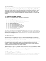
SIXTH FRAMEWORK PROGRAMME SPECIFIC TARGETED RESEARCH PROJECT n° SSPE-CT-2006-044403 AGRIGRID Methodological grids for payment calculations in rural development measures in the EU User Manual for a software tool for creating methodological grids for payment calculations in rural development measures in the EU -- Draft MLURI Team Comments to Kevin Buchan [email protected] Contents 1 Introduction ...................................................................................................................................... 3 1.1 Rural Development Measures.................................................................................................... 3 1.2 Data Libraries ............................................................................................................................ 3 1.3 Multiple Payment Calculations.................................................................................................. 3 1.4 Overview of the Grid Configuration Process ............................................................................ 4 2 Getting Started ................................................................................................................................. 5 2.1 Setup & Installation Issues ........................................................................................................ 5 2.2 Running the Software ................................................................................................................ 6 2.3 Non-Eurozone Currency ............................................................................................................ 6 2.4 Creating a Grid .......................................................................................................................... 6 2.5 Main Grid Window.................................................................................................................... 7 2.6 Editing General Grid Settings.................................................................................................... 8 3 Linkages ............................................................................................................................................ 9 3.1 Data-entry Approaches .............................................................................................................. 9 3.2 Balance Sheet Approach............................................................................................................ 9 3.3 Production Process Approach.................................................................................................. 11 3.4 Creating a Linkage................................................................................................................... 12 3.5 Specifying the RD Commitments ............................................................................................ 14 3.6 Specifying a Baseline .............................................................................................................. 14 3.7 Editing Regulations ................................................................................................................. 17 3.8 Specifying Revenues and Costs............................................................................................... 18 4 Differentiation (of costs and revenues) ......................................................................................... 20 5 4.1 Editing the Library of Differentiation Categories and Elements ............................................. 22 Specifying Values for Costs & Revenues...................................................................................... 23 5.1 Data Entry Using Sub-masks................................................................................................... 24 5.2 Representation of Revenues and Costs.................................................................................... 26 6 Transaction Costs ........................................................................................................................... 27 7 RDR Payment Limits ..................................................................................................................... 28 8 Grid Outputs................................................................................................................................... 29 9 8.1 Viewing Grid Outputs for a Single Calculation....................................................................... 29 Data Libraries................................................................................................................................. 31 1 Introduction This document provides instructions for using the software tool to help develop methodological grids for the calculation of payments in rural development (RD) measures in European Union (EU) member states. The development of the grids focuses on agri-environment measures, natural handicap payments, Natura 2000 payments, forestry measures and animal welfare and meeting standard measures. These grids enable national and regional administrations in the EU and its member states to apply a new harmonised, but at the same time flexible, method for the calculation of payments in the different RD measures. 1.1 Rural Development Measures The software is pre-configured with the following set of RD measures: 131 - Meeting Standards 211 - Natural handicap payments in mountain areas 212 - Natural handicap payments in other than mountain areas 213 - Natura 2000 payments on agricultural land 214 - Agri-environment payments 215 - Animal welfare payments 221 - First afforestation of agriculture land 222 - First afforestation of agroforestry systems 223 - First afforestation of non-agricultural land 224 - Natura 2000 payments on forestry land 225 - Forest-environment payments The software allows the user to define grids for these RD measures with an option to define the grid at the sub-measure level if this is more appropriate. The software does not provide a list of predefined submeasures due to the variability between countries; instead the user can specify the sub-measure during the configuration of the grid (page 6). 1.2 Data Libraries Part of the process of developing a grid involves the repetitive usage of input data such as baseline, differentiation and cost components. In order to facilitate the re-use of these inputs and to reduce the data entry load for the user the software will provide a library for storing this information and will allow the user to easily call upon the information when it is needed. The user will be able to edit library files or share them with other users. The software allows the user to keep multiple libraries and provides the potential for downloading new libraries if they became available. For instance, it might be desirable to keep separate libraries for each country and the user could switch between these libraries to suit the grid in question. When input data from a library is used within a grid the software will create a copy of the data so that the grid file can operate independently of the libraries used to create it. This is essential so users can exchange grid files without the need to have access to the original library file. It also means that users can make changes to the libraries without affecting the existing grid files. 1.3 Multiple Payment Calculations When preparing a grid the software will usually record all costs and revenues within a single payment calculation. For some measures there are separate payments made so, in such a case, the software requires the user to prepare more than one calculation. For example, in the afforestation measures payments are made for: Establishment Costs Maintenance Costs Income Foregone The software has been pre-configured with this information so that when these measures are selected, the software will prompt the user to define all of the necessary calculations. 1.4 Overview of the Grid Configuration Process There are several steps to creating a grid. The user begins by specifying the measure and the data entry approach (balance sheet or production process). Next, they are presented with the main grid window from which they can: Specify the general grid settings (page 5) Configure the payment calculation(s) for the grid View the summary and detailed outputs (page 27) Figure 1 illustrates this process. Specify general settings NEW OPEN Specify measure and data entry approach for each calculation/payment... Main window Create linkages Specify differentiation Specify transaction costs Specify RDR limits Populate grid with cost & revenue values View Outputs Figure 1: grid configuration process The configuration of a payment calculation is broken down into five steps: Creation of linkages which are the relationships between baseline, RD commitment, costs & revenues (page 9) Specification of how the payment is to be differentiated (page 20) Specification of transaction costs (page 27) Specification of RDR limits (page 28) Population of the cost and revenue figures as specified in the previous steps (page 23) 4 2 Getting Started 2.1 Setup & Installation Issues The AGRIGRID software has been designed to run on PC’s running Microsoft Windows. To begin the installation process you must run the setup.exe program that has been provided via download or CD. Depending on the Commission’s preference for a delivery method we could provide a CD containing the software bundle (including documentation) or make the bundle available for download from the AGRIGRID website – or both. The bundle will be provided in English so there is the possibility that we may encounter installation or run-time issues on PCs running with non latin-based character sets. The setup program will prompt you for the installation directory, suggesting the following default1: C:\Program Files\AGRIGRID\ You have the choice of keeping this default or changing it to some other location. The installation directory will contain the following sub-directories: \Documentation\ PDF documentation describing the software and giving examples \System\ Software system files such as executables \Libraries\ Input data files such as baselines and differentiation \Grids\ Output files from the software are called grid files and are stored in this directory You are not tied in to using these folders to store your data files but these will be the default folders that the software will start in when opening or saving data files for the first time. The setup process will provide you with start menu options for viewing documentation and running the software. The documentation will be in PDF format and will require the separate installation of Adobe Reader software2. For convenience, a shortcut to the software will also be placed on the desktop. 1 2 This path may vary from PC to PC – the installation program should detect the correct location for programs http://www.adobe.com/products/acrobat/readstep2.html 5 2.2 Running the Software The first window presented to the user when he/she runs the AGRIGRID software is shown in Figure 2. Figure 2: Starting-up This window is fairly simple - it allows the user to create a new grid or open an existing grid (page 6). It also allows the user to edit the input data libraries (see Data Libraries on page 31). 2.3 Non-Eurozone Currency Some member states are not currently part of the single European currency and as such the calculation of the grids will be done in the local currency (e.g. GBP or CZK). In order to deal with this the AGRIGRID software requires member states to specify the following information: Calculation Currency Exchange rate to Euro In addition to the Euro the software has been pre-configured with the following currencies: Bulgaria - lev (BGN) Czech Republic - koruna (CZK) Denmark – krone (DKK) Estonia - kroon (EEK) Great Britain – pound sterling (GBP) Hungary - forint (HUF) Latvia - lats (LVL) Lithuania - litas (LTL) Poland - złoty (PLN) Romania - leu (RON) Slovakia - koruna (SKK) Sweden - krona (SEK) The calculation (up to and including the inclusion of transaction costs) is performed in the currency specified as the "Calculation Currency". If the "Calculation Currency" is not EUR then the software will use the exchange rate to convert back to Euro before applying the RDR limits which are always specified in Euro. The remaining values are always displayed in Euro. 2.4 Creating a Grid When creating a grid the new grid window (Figure 3) is displayed. Here the user chooses the measure and the data-entry approach. This is the only chance to set these – they cannot be changed later. Figure 3: Creating a new grid 6 Here you should select the measure that is to be considered. You must also consider which approach to take for the entry of cost and revenue components - there are two options. The first is to provide costs and revenues using a balance sheet approach (i.e. following the FADN format). The second is to provide the information in the form of a production process approach. The approaches cannot be mixed or changed so the most appropriate approach must be selected upon this window before proceeding. See Data-entry Approaches on page 9 for more details. 2.5 Main Grid Window The main grid window (Figure 4) is displayed when you create a new grid or open an existing grid. Here you should provide (where applicable) a description of the sub-measure, the country and region (e.g. NUTS3 1 or 2). Figure 4: Main Grid window On this window you can also: Edit further general grid settings Edit the calculation - where the grid for a measure contains more than one calculation the user must first select the one they want (see Multiple Payment Calculations on page 3) View the outputs Save the grid Note: If you wish to prepare a grid that is similar to another then, to save time, open the original grid file, make the modifications and use the ‘Save As’ button to save the grid under a new filename. 3 Nomenclature of Territorial Units for Statistics 7 2.6 Editing General Grid Settings The general grid settings window is shown in Figure 5. It allows you to customise some additional generic attributes for the grid. Figure 5: General Grid Settings In some countries (e.g. Scotland) you may wish to change the calculation currency to the local currency. If so you will also need to ensure that you specify the correct exchange rate to use for conversions between the local currency and the Euro. The ‘Main Calculation Unit’ attribute allows you to specify the main unit for the calculation. The software provides the following options: Ha Livestock Unit Holding . 8 3 Linkages 3.1 Data-entry Approaches You have two data-entry options for providing costs and revenues: Balance sheet approach Production process approach The two approaches cannot be mixed (or changed later in the process) so you must decide which approach to use and select it upon the new grid window (page 6). 3.2 Balance Sheet Approach The Farm Accountancy Data Network (FADN)4 consists of a harmonised annual survey of agricultural holdings carried out by the Member States of the European Union. The balance sheet approach provided by the AGRIGRID software uses the coding system used within the FADN database to organise the costs and revenues (e.g. the code SE350 refers to “contract work”) but does not necessarily expect the user to use the data contained in the FADN database. Figure 6 shows an example of how the revenues and costs associated with a commitment might be recorded using the balance sheet approach. RD Commitment Prohibition of use of any pesticides, fertilisers and soil improvers Baseline Practice Prohibition of use of some types of pesticides Revenues SE195 Forage crops Costs SE295 Fertilisers SE300 Crop protection SE340 Machinery & building current costs SE345 Energy C1 Opportunity cost of family work Figure 6: Data entry using the balance sheet approach Each of these costs and revenues are part of the hierarchical FADN structure5 which is summarised in Table 1. For this approach the software maintains two fixed (i.e. not editable by the user) lists: revenues costs The pre-defined FADN hierarchy shown in Table 1 is intended to help the user understand how the different cost and revenue items are related and will act as a classification system for the balance sheet approach. Items on the left are made up of the sum of those to the immediate right taking into account the + and - signs where appropriate. For example SE415 (Farm Net value added) is equal to SE410 (Gross Farm Income) minus Investments. The items that appear in the revenues list are shown in green while the items that will appear in the costs list are shown in blue. The software will automatically calculate all of the other values (i.e the totals) based on the values that you enter. 4 Farm Accountancy Data Network - the European farming classification system (http://ec.europa.eu/agriculture/rica/index_en.cfm) 5 For further details see the file FADN_Balance_sheet.xls 9 SE135 Total output crops and crop production (+) SE131 Total output SE206 Total output livestock and livestock products SE140 Cereals SE145 Protein crops SE146 Energy crops SE150 Potatoes SE155 Sugar beet SE160 oil seed crops SE165 Industrial crops SE170 Vegetebles and flowers SE175 Fruit SE180 Citrus fruit SE185 Wine and Grapes SE190 Olives and olive oil SE195 Forage crops SE200 Other crop output SE216 Cows milk and milk products SE220 Beaf and veal SE225 Pigmeat SE230 Sheep and goats SE235 Poultry meat SE240 Eggs SE245 Ewes and goats milk SE251 other livestock and products SE256 Other output SE610 Total subsidies on crops Net Income for Justification (+) SE420 Family Farm Income (+) SE415 Farm Net value added (+) SE410 Gross Farm Income SE615 Total subsidies on livestock (+) SE605 Total subsidies (excluding on investments) SE620 other subsidies SE625 subsidies on intermediate consumption SE626 subsidies on external factors SE630 Decoupled payment SE281 Total specific cost (-) SE270 Total inputs SE336 Total farming overheads (-) SE365 Total external factors (-) Investments (allowable by RD paym’nts) SE370 Wages SE375 Rent SE380 Interest SE611 compensatory payments SE612 set aside premiums SE613 other crops subsidies SE616 subsidies dairying SE617 subsidies other cattle SE618 subsidies sheep/goats SE619 other livestock subsidies SE621 environmental subs. SE622 LFA subsidies SE623 Other RD payments SE631 Single Farm payment SE632 Single Area payment SE640 Additional aid SE285 Seeds and plants SE290 Seeds and plants (home-grown) SE295 Fertilisers SE300 Crop protection SE305 Other crop specific costs SE310 Feed for grazing livestock SE315 Feed for grazing livestock (hom.) SE320 Feed for pigs & poultry SE325 Feed for pigs & poultry (home-g.) SE330 Other livestock specific costs SE331 Forestry specific costs SE340 Machinery & building curr. cost SE345 Energy SE350 Contract work SE356 Other direct inputs G100 Forest Land and inc standing timber (-) C1 Opportunity cost of family work Table 1: FADN Hierarchy 10 Should we add a further level of detail? to the right (e.g. brake down Cereals further)? Should we even show this in the user manual? 3.3 Production Process Approach The balance sheet approach, discussed above, considers costs and revenues at a whole farm level. This might not be appropriate in all circumstances so the software provides an alternative production process approach so that the user can group costs within practices (e.g. mowing, fertilisation etc). Figure 7 shows how costs can be grouped within practices to produce a nested structure. RD Commitment (Process) Prohibition of use of any pesticides, fertilisers and soil improvers Baseline Practice Prohibition of use of some types of pesticides Revenues Revenue 1 Costs Fertilisation (practice) + Cost 1 + Cost 2 + Cost 3 Crop protection (practice) + Cost 4 + Cost 5 Figure 7: Data entry using the production process approach (a) An additional benefit of having this nested structure is that you have the option of providing values at the practice level or at the cost level depending on the availability of data. If you specify values for the costs then the software will automatically calculate the values for the practice. It may not always be possible to associate costs with a practice so costs can be defined without being nested within an practice (Figure 8). RD Commitment (Process) Production of organic cereals Baseline Practice Production of conventional cereals Revenues Revenue 1 Revenue 2 Costs Cost 1 Cost 2 Cost 3 Figure 8: Data entry using the production process approach (b) It is also valid to nest some costs within a practice while specifying some costs without a practice. The software maintain three lists for the production process approach: revenues activities (including nested costs) costs The components within the production process lists are classified (e.g. crop, forestry, livestock) in order to filter the lists during grid configuration. For instance, the user might wish to select the ‘forestry’ classification in order to show only forestry related activities, costs and revenues. You can modify the lists used for the production process approach but not the lists used for the balance sheet approach. 11 3.4 Creating a Linkage The AGRIGRID software defines a linkage as the combination of an RD commitment, a related baseline, a set of revenues and a set of costs (optionally nested within practices - production process approach only). The window shown in Figure 9 is used to configure the linkages for a payment calculation. Figure 9: Linkage window with second linkage selected The linkages are summarised in the window. The idea is that the software will help the user to create the grid in a logical manner by building up and organising a list of linkages that apply to the calculation. If you click the New button the software will create a new linkage. If you select one of the linkages and click Modify the software will allow you to edit the selected linkage. The Delete button lets you delete the selected linkage. Changes to a linkage are performed in the linkage window shown in Figure 10. 12 Figure 10: Creating a new Linkage There are two mandatory steps to configuring a linkage: Specify the RD Commitment (page 14) Specify the baseline (page 14) Then, depending on the approach being followed, you must enter revenue and cost information as described in the following sections: Specify revenues and costs (page 18) – balance sheet approach Specify revenues, activities and costs (page 18) – production process approach As noted earlier (Data-entry Approaches on page 9), the production process approach allows you to define costs on their own or within practices. 13 3.5 Specifying the RD Commitments You can specify the RD commitment by clicking the set button next to the RD commitment attribute in Figure 10. This displays the RD Commitment window shown in Figure 11. If the desired entry is not in the list then the user can use the New button to create a new entry in the library. Figure 11: Editing and Selecting Rural Development Commitments The RD Commitments are tied into each RD Measure so the software will maintain separate lists for each measure – and therefore only display those commitments that apply to the measure in question. 3.6 Specifying a Baseline To configure a baseline within the software you should click the set button situated next to the baseline attribute (Figure 10). This launches the window shown in Figure 12. 14 Figure 12: Window for setting a baseline The purpose of this window is to help us identify the baseline (or reference level). The software represents two types of baseline: common practice and a baseline based upon one or more regulations. For the regulatory baselines, there are three types: Statutory Management Requirements (SMR) Good Agricultural and Environmental Conditions (GAEC) Additional (Regional) Baseline You can specify a title and select the type of baseline (i.e. common practice or regulatory). If it is a regulatory baseline then you should also select the regulations that apply by clicking New – this displays the list of regulations (Figure 13). If necessary you can supersede regulatory baselines with more restrictive common practices – this is easily achieved by selecting the regulations that apply, setting the type attribute to ‘Common’ and using the notes attribute to explain how the regulations are being exceeded. In a similar fashion, the notes attribute could also be used to indicate when only part of a regulation applies. 15 Figure 13: Baseline regulations If the relevant regulations are not in the library you can create or edit an entry (see Editing Regulations on page 17), or use the Library button to open a different library in order to locate the regulation. When the user clicks the ok button in the software will record the changes and return to the linkage window. 16 3.7 Editing Regulations The regulations window is shown in Figure 14. Figure 14: Regulation window It is fairly simple and allows you to provide a type categorisation for the regulation, a short title and a larger section that can be used to describe the regulation in more detail. A sample set of SMR, GAEC and additional regulations will be provided in the supplied regulation library; however you can supplement the library with the regulations that apply in your country/region. 17 3.8 Specifying Revenues and Costs The user specifies a new cost or revenue by clicking the new button next to the cost or revenue box shown in Figure 10. Figure 15 shows the windows for selecting a revenue component using the balance sheet approach. Figure 15: Selecting Costs and Revenues for Balance Sheet Approach To help with navigation you can use the + and – buttons to explode and contract the hierarchy. With the balance sheet approach the software will allow you to specify the same costs and revenues within different linkages; however they will only be included once in the final calculation. For the production process approach the procedure for adding costs and revenues is similar. Figure 10 shows an example of adding a practice/cost. 18 Figure 16: Selecting Practices/Costs for Production Process Approach Select the practice or cost that you require and click Ok to include it in the linkage. If the desired entry is not provided in the list then you can use the new, edit and delete controls to modify the contents of the pick-list. The cost and revenue lists for the production process approach are nested within their classifications to help you to find the component you are searching for. 19 4 Differentiation (of costs and revenues) Differentiation is the criteria under which an RD payment is distinguished. By specifying differentiation categories within the software you can create a series of alternative scenarios for a payment calculation. A differentiation category such as type of trees is defined to contain a series of differentiation elements such as conifer or native woodland. The software provides a mechanism for differentiating payment based on the specification of one or more these categories and elements. Note: Differentiation elements must not be confused with the different cost/revenue components used in the calculation of an individual payment. e.g. If a RDP states that a payment is different for cereals and industrial crops, then these two types of crop are differentiation elements; however if cereals and industrial crops are characterised by the same payment but the calculation refers to both crops (e.g. calculating the average value of cost/revenue), then the two types of crop cannot be considered as differentiation elements. Also, eligibility criteria (e.g. minimum area under contract, or payments granted only for NVZs) cannot be considered as differentiation elements. If the payment calculation is to be differentiated then the first step that you need to take is to click the Edit button labelled Differentiation of Payment Calculation upon the Payment Calculation window (see Creating a Linkage on page 12). This displays the differentiation window shown in Figure 17. Figure 17: Differentiation The top of the window shows the list of differentiation categories that are included in this grid. When a selection in made here the bottom part of the window shows the elements that are contained within the selected differentiation category. Ticks indicate that an element is in use – clicking a differentiation element toggles the tick on and off. Switching off unnecessary elements is useful especially when there are a large number of categories and elements being considered. The elements in each of the differentiation categories act as multipliers so 20 that 3 categories that each contains 6 elements give 6x6x6 = 216 different possibilities! For this purpose the software gives an indication of the number of combinations that will be created. Add new categories to the grid using the New button – this displays the window shown in Figure 18. Figure 18: Selecting a differentiation category Note: Once a category has been imported it cannot be altered and subsequent changes to the library will not appear in the imported categories. This is because the grid makes a copy of the differentiation category when it is added since it needs to maintain the referential integrity in the absence of the original library file. You should ensure that the differentiations have been set correctly before proceeding to enter values for differentiated costs and revenues (see Specifying Values for Costs & Revenues on page 23) since subsequent changes may lead to the loss of some values. The user will be warned about this when making changes to the differentiations in order to avoid accidental deletion of data. 21 4.1 Editing the Library of Differentiation Categories and Elements The software has been pre-configured with differentiation categories and elements but you can edit these or create your own. Figure 19 shows the window for editing a differentiation category. Figure 19: Differentiation category 22 5 Specifying Values for Costs & Revenues Once the grid calculation(s) have been configured the user is ready to begin entering values for each of the cost and revenue components. When you click Next on the Payment Calculation window you will proceed to the Populate Grid window shown in Figure 20. Figure 20: Entering values for each differentiation On the left, the window shows the list of costs and revenues that you configured earlier. Selecting one of these costs or revenues displays the data values grid on the right. The data grid shows a row for each of the differentiation combinations based on your configurations in the payment calculation differentiation editor (see Differentiation (of costs and revenues) on page 20). Each row contains a description of each of the differentiations that it applies to, a value for baseline, commitment and the difference between the two. Finally there are three buttons. The details button allows you to specify detailed information for this data row. The copy and paste buttons allow you to copy one set of data (including underlying sub-mask formulas and comments) and paste it into another row – useful if some differentiations share the same data values. The user has three data-entry options: Specify a baseline and RD commitment and leave the software to calculate the difference (i.e. the additional commitment) Specify the difference directly (first need to click Details and change the mode) Click Details to open the more detailed component editor (Figure 21). 23 Figure 21: Cost component window This window shows the payment calculation, component and differentiation that is being considered. You can provide detailed notes or comments. You then have the choice of specifying the values for baseline and RD commitment directly or by specifying a sub-mask. The additional commitment will be automatically calculated by the software, however if no baseline and RD commitment is available the user will be able to specify the value directly by switching on the Specify Additional Commitment directly option. It is advised that you should always record the data source. Rather than just specifying a value directly in is often more appropriate to specify a lower level of detail in the form of a formula. To do this you need to create a sub-mask by clicking the corresponding Edit button. The Clear button removes the sub-mask and reverts to specifying the value directly. When a sub-mask is configured these buttons will appear in light yellow. 5.1 Data Entry Using Sub-masks The sub-mask window (Figure 22) provides you with space to provide a title for the calculation and to provide the formula and details of the elements that make up the formula. The software will calculate the result, display it at the bottom and return this to the component window. 24 Figure 22: Sub-mask window Add and remove formula elements using the Add and Delete buttons. Once you have specified values for all of the elements and prepared the formula clicking Calculate invokes the software to express the formula as values and then as a final result. If there are any problems with the formula syntax then the software will attempt to give appropriate details so that you can correct the error. The real power of the sub-mask editor is its recursive capabilities. This means that an element in one formula can be derived from another sub-mask and inside the new sub-mask another element could be derived from a further sub-mask. Theoretically there is no limit to the number of nested sub-masks that are allowed although it will become difficult to manage. If the user opts to use a sub-mask (SM2) to calculate a value in a sub-mask (SM1) then the software would automatically calculate the result of SM2 and display it for the relevant value in SM1. Light yellow buttons indicate the use of a sub-mask to calculate a value. Another example of where the sub-mask can be useful is when a value is calculated based on a multipleyear average. Here the user could build a formula to calculate the mean value from many yearly separate figures. By doing it in a sub-mask the workings are recorded as part of the grid file for later reference. Formulas can be saved to the library for re-use later. When the user creates a new formula it can be added to the library using the Save to Library button. The Sub-mask library button allows the user to browse previously defined formulae and select one for use. 25 5.2 Representation of Revenues and Costs When configuring a grid it is useful to understand how the software deals with revenues and costs. You enter costs and revenues as absolute/positive values but the software deals with them differently as denoted by the formulae: income loss = baseline income – commitment income additional cost = commitment cost – baseline cost The following three scenarios illustrate how this will work in practice. Scenario 1: This is the most frequent situation. The observance of the additional commitments generates a decrease of farm income (reduced from € 100 to € 80) and an increase of production costs (from € 50 to € 75). So, the calculation of the RD payment (additional costs + income loss) is represented by two positive figures (€ 20 and € 25). Revenue Costs Gross Income Baseline € 100 € 50 = 50 Commitment € 80 € 75 = 5 Income Loss (baseline - commitment) € 20 + € 25 = € 45 Additional Cost (commitment - baseline) Payment Figure 23: Representing Revenue and Cost Values - Scenario 1 Scenario 2: Here the observance of the additional commitments means an increase in farm income (from € 100 to € 110) resulting in a negative income loss of - € 10. Revenue Costs Gross Income Baseline € 100 € 50 = 50 Commitment € 110 € 75 = 35 Income Loss (baseline - commitment) Additional Cost (commitment - baseline) Payment - € 10 + € 25 = € 15 Figure 24: Representing Revenue and Cost Values - Scenario 2 Scenario 3: In this situation the observance of the additional commitments produces a decrease of the costs (from € 50 to € 30) resulting in a negative additional cost of - € 20. Revenue Costs Gross Income Baseline € 100 € 50 = 50 Commitment € 50 € 30 = 20 Income Loss (baseline - commitment) Additional Cost (commitment - baseline) Payment € 50 + - € 20 = € 30 Figure 25: Representing Revenue and Cost Values - Scenario 3 26 6 Transaction Costs When you click Next on the Populate Grid window you will proceed to the Transaction Costs window shown in Figure 26. Figure 26: Transaction Costs This window lists the transaction costs that have been configured for the grid. There are two modes: percent and fixed value – only one type is allowed per grid, the two cannot be mixed. The New, Edit and Delete buttons allow you to edit the transaction costs list. Figure 27 shows the editor for transaction costs. Figure 27: Transaction costs editor Transaction costs as a percentage of gross income are limited to a maximum 20% (in total) and the software will not allow the user to exceed this. It is not possible to restrict the fixed amount transaction cost at this stage since we do not yet know how much the gross income will be however the final calculation will enforce a maximum of 20% for the total of all transaction costs. 27 7 RDR Payment Limits When you click Next on the Transaction Costs window you will proceed to the RDR Payment Limits window shown in Figure 28. Figure 28: RDR Payment Limits editor RDR payment limits allow you to set a rate, minimum and maximum value for the payments. The software also allows you to differentiate the limits. The example shows five differentiations for the RDR limits. You can specify the values for rate, minimum and maximum directly. Although it is unlikely that all three RDR limits will be applied simultaneously, for technical purposes the following precedence is applied within the software: RDR Rate (applied first), RDR Minimum and RDR Maximum (applied last). 28 8 Grid Outputs 8.1 Viewing Grid Outputs for a Single Calculation Once the grid has been configured the user can proceed to the outputs window shown in Figure 29. Figure 29: Grid outputs window showing single calculation (balance sheet approach) On the left of the window is a tree structure showing all of the valid combinations of differentiation elements. Selecting a ‘leaf node’ (i.e. an element at the end of the hierarchy) and clicking the Show button displays the calculation for that differentiation on the right of the window in a spreadsheet style format. You can display as many calculations as you like. The data on the right can be selected, copied (Ctrl-C) and pasted into Excel for further analysis. The outputs window also has options for modifying the display of data such as setting the level of detail that is visible. The difference in gross income is the sum of the income forgone and additional costs. Transaction costs are applied to the gross income figure, either as an additional amount or as a percentage. The software will limits to the sum of the transaction costs to 20% of gross income. 29 Overall financial support is calculated as the sum of gross income and transaction costs after any RDR adjustment such as RDR rate. When many differentiated calculations are displayed a sideways scroll bar may also appear since the output can become very wide. If the grid contains multiple calculations (i.e. for the forestry measures) the software will prepare the calculations as separate payments and will show a total for all three payments for information purposes. 30 9 Data Libraries You can edit the data libraries at any time by clicking the Library button on the start-up window (see Getting Started on page 5). This action displays the window shown in Figure 30. Figure 30: Data libraries The window contains shortcuts to all of the input data libraries that have been discussed earlier in this document but with the advantage of having them all accessible in one place. Clicking the Config button displays the library management window shown in Figure 31. This window allows you to perform operations such as creating a new library, switching to another library or saving the library. Figure 31: Library management 31