Download User Manual

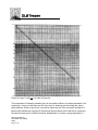
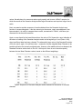
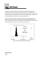
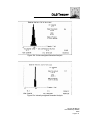
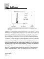
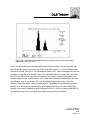
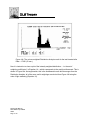
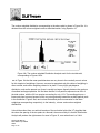
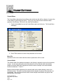
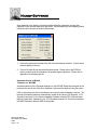
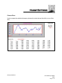
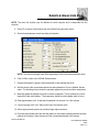
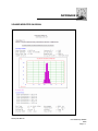
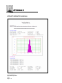
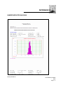
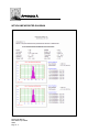
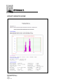
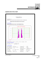
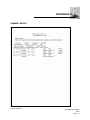
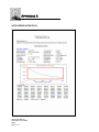
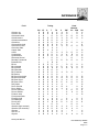
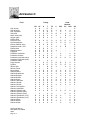
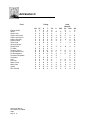
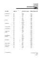
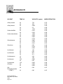
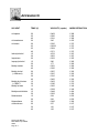
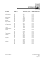
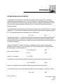
D LS T h e o r y
The results shown in Table 1 for a well-behaved fat emulsion nicely illustrate some of the
characteristics of the Gaussian Analysis, discussed earlier. First, we notice that the parameter
Chi Squared cannot be used to judge the stability and/or quality of the fit results if too little data
has been acquired. Here, just 31 seconds into the run, the very low value of Chi Squared is
potentially misleading in suggesting that the Gaussian Analysis has already produced final”
results, of high quality, with settled values of the Mean Diameter and Standard Deviation. In
fact, Chi Squared later increases, to a high of 2.8 at the later time of 8 min 4 see, when
substantial amounts of additional Data have been incorporated into the autocorrelation function
(564K in Channel #1). However, what is meaningful is the fact that this rise is obviously
spurious, since it is followed by consistently lower values; Chi Squared falls back essentially to
unity (1.1) after 13-14 minutes into the run. Clearly, what matters in establishing the validity of
the Gaussian Analysis result for this sample is the fact that Chi Squared remains low with
increasing data acquisition, showing no tendency to grow with time.
Second, we verify from Table 1 that the intensity-weighted Mean Diameter (colt 3) settles very
quickly to a reliable value. After just a couple of minutes, all succeeding values are within 1 % of
the “settled” value of approximately 226nm. On the other hand, the exhibits considerably initial
few minutes of difference is the fact the “settled” value of approx. 226 nm. volume-weighted
Mean Diameter (col. 5) more variation (up to 4%) during the data acquisition. The reason for this
that the Standard Deviation has not yet settled to a constant value. Clearly, a higher degree of
statistical accuracy (i.e. signal/noise ratio) is required in the autocorrelation function to establish
the value of the “curvature” coefficient, a2, in the least-squares quadratic fit (Equation 11), than
is needed to fix the value of the linear coefficient, a1. Consequently, early into the run, we
observe a 20% variation in the Standard Deviation (coming from a2), as opposed to less than a
2% fluctuation in the intensity-weighted Mean Diameter (from a1).
This affects the results in two ways. First, the relatively large values of the Standard Deviation
(30 to 35% of the Mean Diameter) serve to “push” the volume-weighted Mean Diameter fully
10% below the intensity-weighted value, to approximately 209 nm. Second, because of the
substantial fluctuation in the computed Standard Deviation in the early stages of data
acquisition, the volume-weighted Mean Diameter fluctuates considerably more than does the
intensity-weighted value. However, regarding these fluctuations, a simple rule applies: allow
more time! Obviously, the sample represented in Table 1 is rather well behaved, requiring no
Baseline Adjust and yielding good results very early into the run, close to the final, settled
Nicomp 380 Manual
PSS-380Nicomp-030806
06/06
Page 2 - 38