1
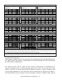
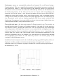
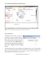
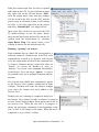
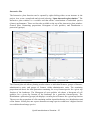
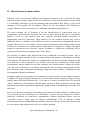
A quick introduction to Zonation........... Version 1 (for Zv4) Enrico Di Minin Victoria Veach Joona Lehtomäki Federico Montesino Pouzols Quick introduction to Zonation - 1 Atte Moilanen Quick introduction to Zonation - 2 Table of Contents — A Quick Introduction to Zonation 1. What is Zonation? ................................................................................................. 5 2. Scope and aims of this document .......................................................................... 5 3. What is Zonation useful for? ................................................................................. 5 4. Who can use Zonation? ......................................................................................... 6 5. Why is Zonation different from other tools? ........................................................ 7 What can Zonation be confused with? ................................................................... 7 What about other software intended for approximately the same purpose? .......... 7 6. How does Zonation work? .................................................................................... 9 7. About data ........................................................................................................... 12 8. How to do a simple Zonation run........................................................................ 13 The project file (.bat) ........................................................................................... 14 The feature list file (.spp) ..................................................................................... 14 The run settings file (.dat) .................................................................................... 15 9. How to interpret Zonation main output............................................................... 17 Performance curves .............................................................................................. 18 The priority rank map .......................................................................................... 18 10. The Zonation Graphical User Interface (GUI) .................................................. 19 Project Management ............................................................................................ 19 Console view ........................................................................................................ 21 Visual Output ....................................................................................................... 21 Text output ........................................................................................................... 22 Runtime plot......................................................................................................... 23 Merged Map ......................................................................................................... 23 Interactive Plot ..................................................................................................... 25 11. What Zonation has been used for ...................................................................... 26 12. Some core references ........................................................................................ 27 13. Where to get more information ......................................................................... 28 14. Credits & brief history ...................................................................................... 29 Quick introduction to Zonation - 3 This guide is a product of C-BIG, the Conservation Biology Informatics Group, at the University of Helsinki Version 1 — 2014 ISBN: 978-952-10-9921-2 (paperback) ISBN: 978-952-10-9922-9 (PDF) Unigrafia OY, Helsinki Quick introduction to Zonation - 4 1. What is Zonation? Zonation is a publically available decision support system for spatial conservation planning. It is special-purpose software built for solving various problems around spatial conservation resource allocation, and it is capable of data rich, large scale, high resolution spatial conservation prioritization. Zonation is a set of methods and analyses implemented in one package, and, compared to many other software programs with similar purpose, has the broadest analysis options available for spatial conservation planning. 2. Scope and aims of this document This manual was written to provide a quick and (relatively) simple explanation about what Zonation is, what it is not, who can use it, and what it can be used for. We also summarize the basics of getting started with using Zonation. We make reference to further literature where relevant. 3. What is Zonation useful for? There are many potential uses for Zonation, and many examples of its use already exist in scientific literature. All the following analyses are possible with suitable inputs and interpretation of outputs. Please see the user manual and scientific literature for description of how Zonation analyses are typically set up and the associated case studies. Standard usages (possible with simple setups) Reserve selection. Identification of the best part of the landscape (~reserve network) that produces high return on investment and balanced outcome across all biodiversity features. Reserve network expansion. Identify the optimal balanced expansion of an existing reserve network. Can account for connectivity if desired. Evaluation of an existing or proposed conservation area network. Comparison between how good it is and how good it could have been. Impact avoidance. Identify areas where economic development leads to limited ecological losses. Balancing of alternative land uses. Balance between many biodiversity features and the needs of several alternative land uses (opportunity costs). Target-based planning. Solution of the minimum set coverage problem, i.e., how to satisfy your targets with minimum cost. Quick introduction to Zonation - 5 Advanced usages (with higher data requirements or more complex analysis setup) Biodiversity offsetting. Find areas that best compensate for ecological damage: how to expand the existing reserve network in a balanced manner to compensate for specific losses. Planning under climate change. Use present distributions and future distributions of biodiversity features, as well as connectivity between the present and future distributions to identify current and future areas of relevance. Targeting of habitat restoration or habitat management. Modeling of "difference made" by management/restoration is accounted for in a complicated and data demanding analysis. 4. Who can use Zonation? Zonation is available for free and can be used by anyone. Those working in conservation management, research, teaching, consulting, universities, NGOs, etc. may be interested in this software. There are no restrictions on the use of the software, except that the appropriate scientific references describing the methods used should be made in documents and presentations. While the Zonation software itself does not come with a license fee, there nevertheless is a price associated with using it. The time needed to understand and use the methods can, in fact, be quite long. Additionally, collating the input data is frequently a very time-consuming phase. Thus, Zonation is not a free lunch "do it all in a day" solution into spatial conservation planning. The structure of a Zonation project, resources needed, risks, and opportunities perceived by stakeholders are discussed in the open access article by Lehtomäki and Moilanen (2013). Zonation can be used by anyone working in systematic conservation planning, spatial conservation prioritization, reserve selection, site selection, reserve network design, or spatial conservation planning and related fields in general. Zonation can also be applied in the context of other land use planning where the focus is not on biodiversity conservation. While different methods and software implementations may have different strengths, we encourage you to compare alternatives in terms of the analytical options offered, size of data that can be analyzed, ease of use, etc. Zonation is also useful for teaching about spatial conservation prioritization. The Zonation v4 graphical user interface (GUI) is easy to use, and can also be used for investigating and visualizing input data. Quick introduction to Zonation - 6 5. Why is Zonation different from other tools? There are two topics to cover here: software intended for completely different purposes and software intended for approximately the same purpose. What can Zonation be confused with? Zonation is not software for statistical species distribution modeling (SDM), like e.g. MaxEnt1 or BIOMOD2. In SDM, information about environmental variables is statistically related to conditions at locations where a species has been observed to occur. The outcome is a species distribution model that extrapolates the expected occurrence level of the species across the landscape. Zonation does not do SDMs. However, Zonation can use many SDM-generated rasters as input layers. Neither is Zonation a software for stochastic spatial population viability analysis (SPVA), such as RAMAS3. Like outputs from species distribution models, the output of a SPVA (e.g. predictions species extinction risks) could be used as input for Zonation. Zonation is about synthesizing information across many – potentially very many – species and other biodiversity features. While Zonation does include many connectivity features, it is not software primarily intended for analysis of connectivity; it accounts for connectivity in prioritization. Zonation integrates habitat quality, habitat area, and connectivity for many biodiversity features simultaneously. It can also account for many costs and opportunity costs and other considerations. See Hodgson et al. (2009) about the role of connectivity in conservation. While Zonation v4 graphical user interface has much improved capabilities in visualizing the spatial input and output data (e.g. rasters), it is not a GIS software. You can easily view input raster data and do simple overlay analysis for the resulting spatial data (e.g the priority rank rasters), but Zonation is not truly spatially-aware (i.e. there is no support for projections and coordinate systems) and you cannot import additional spatial data. Zonation does not deal with vector data at all. What about other software intended for approximately the same purpose? The most direct comparison is to software intended for systematic conservation planning or spatial prioritization, including programs such as Marxan4, Marxan with zones5, ConsNet6, CPlan 7, etc. Also relevant is comparison to integer-programming (IP) implementations meant 1 http://www.gbif.org/resources/2596 https://r-forge.r-project.org/R/?group_id=302 3 http://www.ramas.com/ramas.htm 4 http://www.uq.edu.au/marxan/ 5 http://www.uq.edu.au/marxan/latest-r-d 6 http://uts.cc.utexas.edu/~consbio/Cons/consnet_home.html 7 http://www.edg.org.au/free-tools/cplan.html 2 Quick introduction to Zonation - 7 for solving target-based reserve selection problems. Comparing software with different conceptual underpinnings and only partly overlapping objectives is far from trivial. Thus, the reader should consider the following as just a few general pointers and not as an exhaustive review. Do an up-to-date comparison and see what fits the purpose of your work best. There are major differences between Zonation, Marxan (with and without zones), and ConsNet. Marxan variants and ConsNet are intended for target-based planning, in which the typical aim is to achieve feature-specific targets with minimum cost. This aim implies that feature-specific targets first need to be set, a process that in itself leads to lowered return on conservation investment (see Laitila and Moilanen 2012). While Zonation can do target-based planning perfectly well 8 , it also includes what can be called higher-level models of conservation value. These models apply more generic principles about how conservation value is aggregated across features, space, and possibly time. Application of these generic principles leads to a balanced priority ranking, which arises as an emergent property of the principles and input data. As such, the mode of operation is very different from target-based planning, in which the solution is in a sense defined a-priori, via the targets. Another major difference between Zonation and Marxan are the outputs. Marxan produces a solution for the minimum set coverage problem, i.e., which areas satisfy your goals with minimum cost. Zonation produces a balanced priority ranking, in which top and bottom fractions of the landscape can be seen at the same time. Also, a range of conservation investments can be investigated rather than having a result for one target set. There are also other major differences. Zonation is deterministic and can operate on very large rasters (v4 up to the order of 100 million elements). Marxan operates on polygon vector data and is stochastic, giving a different result each run. Marxan has required input data to be classified into presence-absence (1/0), while Zonation does not. There also are differences in how well the approaches can account for connectivity, uncertainty, land use restrictions, multiple costs, etc. All and all, there are great conceptual and practical differences between Zonation and the other software intended for similar purposes. Please make a comparison for yourself. Marxan with Zones differs from the methods cited above in that it seeks options over multiple different allocations for each planning unit (polygon). Allocation of different land uses has different costs and consequences for different features. This is not a feature directly supported in Zonation. See also the RobOff 9 software for development of portfolios of conservation action across environments. Integer programming (IP) methods are often too focused on globally optimal solution of specific problems while forgetting the realism of the problem formulation. Limitations of IP formulations have included (and these may not apply to all problem variants and solution methods): requirement of binary (presence-absence) input data, applicability of limited 8 Zonation applies to efficient target-based planning, including the combined targets and benefits planning outlined in Laitila and Moilanen (2013). 9 http://cbig.it.helsinki.fi/software/roboff/ Quick introduction to Zonation - 8 connectivity methods only, and applicability limited to small-medium sized data. In any case, IP formulations are about target-based planning, and the comments about lowered return on investment apply as well. 6. How does Zonation work? The high-level of Zonation Sections 6-8 operation here include somewhat more detailed information about Zonation. If you simply want to try it out, you can skip to Section 10 about the Zonation graphical user interface. It may also be useful to then look at Section 9 about interpretation of outputs. Compared to other conservation planning tools, Zonation produces a complementarity-based and balanced ranking of conservation priority over the entire landscape (Moilanen et al. 2005), rather than satisfying specific targets at minimum cost. On the right there is a summary of the flow of computational operations in Zonation. The priority ranking is produced by iteratively removing the grid cell or planning unit that leads to smallest aggregate loss of conservation value, while accounting for total and remaining distributions of features, weights given to features, and feature-specific connectivity. Here, “grid cell” means a pixel on a map. Zonation uses a raster for each biodiversity feature, where each cell (pixel) contains a number for the occurrence level of that feature. The way loss of conservation value is aggregated across features (occurring in a cell) depends on the so-called cell-removal rule. Iterative priority ranking starts from the full landscape and removes cells, stepwise minimizing loss, until there are none remaining. Least valuable cells (e.g. a few common species occurring) are removed first, while the most important cells for biodiversity (e.g. high species richness and species occurrence) are kept till the end. These calculations are illustrated in the table on the next page. Models of conservation value While the Zonation algorithm is the same under all analyses, there are conceptually different models of aggregating conservation value. All these models give highest priority for locations with high occurrences for many rare and/or highly weighted species. Low priorities go to areas where there is a small number of common, widespread features, "parking lots". Between these similarities, there are differences in how much emphasis is given to many features versus rare features. Quick introduction to Zonation - 9 1. Input three 5x5 "species distributions" Spp A - presence-absence data B - probabilities of occurrence weight = 2.0 weight = 1.0 1 1 1 1 1 0 1 1 0 1 0 0 0 0 0 Sp A sum of elements =8 0 0 0 0 0 0 0 0 0 0 0.9 0.98 0.1 0 0.9 0.98 0.1 0 0.5 0.4 0.01 0 0.5 0.1 0.01 0 0.5 0.1 0.1 0 Sp B sum of elements = 6.18 C - abundance weight = 3.0 0 0 0 0 0 1 1 1 1 0 0 0 0 0 0 Sp B sum of elements 2 2 2 0 0 = 72 8 7 5 5 2 9 12 7 5 2 0.111 0.097 0.069 0.069 0.028 0.125 0.167 0.097 0.069 0.028 2. Convert (normalize) to fraction of distribution in cell. 0.125 0.125 0.125 0.125 0 0.125 0.125 0.125 0 0 0.125 0 0 0 0 0 0 0 0 0 0 0 0 0 0 0.146 0.146 0.081 0.081 0.081 0.159 0.159 0.065 0.016 0.016 0.016 0.016 0.002 0.002 0.016 0 0 0 0 0 0 0 0 0 0 0.014 0.014 0 0 0 0.014 0.014 0 0 0 0.028 0.028 0.028 0 0 3. Multiply by feature weights to get weighted fraction of distribution in cell. Lowest & highest scoring cell shaded. 0.25 0.25 0.25 0.25 0 0.25 0.25 0.25 0 0 0.25 0 0 0 0 0 0 0 0 0 0 0 0 0 0 0.146 0.146 0.081 0.081 0.081 0.159 0.159 0.065 0.016 0.016 0.016 0.016 0.002 0.002 0.016 0 0 0 0 0 0 0 0 0 0 0.042 0.042 0 0 0 0.042 0.042 0 0 0 0.083 0.083 0.083 0 0 0.333 0.292 0.208 0.208 0.083 0.375 0.500 0.292 0.208 0.083 4. Hypothetical distributions after several iterations when several cells have been removed (marked in dark grey) 1 1 1 1 1 0 0 0 0 0 Sp A remaining sum = 5 0.9 0.9 0.5 0.98 0.98 0 0 Sp B remaining sum = 4.26 0 0 0 1 1 0 1 1 8 7 9 12 7 0.511 0.447 0.574 0.766 0.447 Sp C remaining sum = 47 5. Weighted fraction of remaining distribution in cells has now changed. 0.4 0.4 0.4 0.4 0.4 0 0 0 0 0 0.211 0.211 0.117 0.230 0.230 0 0 0 0 0 0.064 0.064 0 0.064 0.064 6. At this stage Additive Benefit Function (ABF)*would remove from the right-side cluster (cells with 0.447) and Core-Area Zonation (CAZ) from the left. At the left, either connectivity or 2nd highest species occurrence would point to the shaded cell. With ABF, at the right, connectivity would break the tie between the two cells with 0.447. 7. Calculations such as illustrated above are used together with connectivity considerations and costs to determine the next cell to remove.Remaining area is then updated and the process returns to step 4. Iteration recurs until no cells (or planning units) remain. † See next section for the Core-Area Zonation (CAZ) and Additive Benefit Function (ABF) models for aggregating conservation value. *This example is simplified in that it is not shown how the benefit functions enter the ABF calculations. In fact, ABF does not do the range-size renormalization, but increasing marginal losses when representation goes down amount to a similar effect. The additive-benefit function (ABF) has the heuristic interpretation of minimization of expected extinction rates via feature-specific species-area curves. It sums the loss across features, converted via feature-specific benefit functions. Because it sums, it implicitly ends up giving high importance to cells with many features in them (that is, high species richness) of course tuned by local occurrence levels and weights of features. With the ABF, gains in Quick introduction to Zonation - 10 conservation value level off when coverage for a feature increases, which introduces a balance (~complementarity) that it is preferable to have representation of all features in the solution. Core-area Zonation (CAZ). Instead of a sum, CAZ bases ranking on "the most important occurrence of a feature in the cell". Therefore, it is able to identify as high-priority areas that have a high occurrence level for a single rare and/or highly weighted feature. Even generally feature-poor cells can thus be identified as priorities. Difference between ABF and CAZ. The difference between ABF and CAZ is effectively the same as between a mean and a maximum, taken from a set of numbers, which here are the feature-specific scores that are basis for deciding which cell to remove next. Compared to CAZ, ABF tends to produce a higher average proportion of feature distributions retained, but smaller minimum. This is because relatively feature-rich areas may be favoured at the expense of some features occurring in generally feature-poor areas. Note that the choice between ABF and CAZ is not a binary black-and-white choice between richness and rarity, it is more about a tendency between emphasis on richness and the need to cater for all features. For example, countries like UK or Canada would have highest species richness in the south, but there nevertheless are some species that only occur in the north. CAZ pays relatively higher attention to core locations of the northern species, with the unavoidable price of reduced priorities in the south. The difference between ABF and CAZ is case-specific and depends on how feature distributions are nested. In target-based planning, Zonation calculates the traditional minimum set coverage solution as part of the priority ranking. The minimum set solution can be extracted from the priority ranking right before the first target is about to fail with the removal of the next grid cell from the landscape. In Zonation, target-based planning uses a special benefit function designed for the purpose. We refer to the Zonation user manual for a full explanation on the other two cell-removal rules (generalized benefit function and random cell removal). Here we provide a short video about how different types of cell removal work in Zonation. Connectivity Zonation can (presently) account for connectivity in eight ways, which are summarized in the table below. Compared to many other conservation planning tools, Zonation can uniquely account for feature-specific connectivity at large extents using very fine resolution data. For example, with distribution smoothing, the widths of the kernels can describe either the dispersal capability or scale of landscape use of the species (related to home range size). Connectivity method edge removal BLP - Boundary length penalty Type structural structural Brief characterization Usually used; retains some continuity; speeds computations. Most common connectivity method in reserve selection. Reduces the edge-to-area ratio of remaining areas. Quick introduction to Zonation - 11 distribution smoothing feature-specific BQP Boundary quality penalty NQP – Directed connectivity feature-specific interaction connectivity between pairs of features matrix connectivity amongst many partially similar habitats corridor connectivity tries to retain corridors during ranking feature-specific Metapopulation-type, declining-by-distance connectivity measure. Can be tuned according to the needs of each feature. Identifies areas with a high density of highquality habitats. More highly parametric feature-specific response. Updated iteratively during ranking. Slows computations. Extension of the BQP for a tree-like river system, with connectivity responses both up and down the river. Requires specification of linkages between planning units (catchments). Like distribution smoothing but computed between either as positive or negative between two distributions. Can be e.g., between predator and prey, or between present and future. Recognizes that partially similar habitats that share many species help each other's connectivity. For example, different forest types could help each other's connectivity. Maintains corridors during the ranking. Width and strength of preference for corridors can be tuned. All of these connectivity methods have their uses (see user manual), but connectivity does not need to be used always: use of it is optional. Frequently, an analysis without connectivity is informative already, and simple application of the BLP, distribution smoothing and interaction connectivity could go a long way in including realistic connectivity effects. 7. About data Zonation is applicable to analysis of data about distributions of biodiversity features, such as species, ecosystems, environment types or habitats, accounting for current occurrence and possibly their future expected state dependent on conservation intervention. In addition, Zonation can account for data about the spatial distribution of socio-economic factors relevant for finding conservation opportunities. The numbers inside the data layers can be any nonnegative numbers; presence-absence, probability of occurrence, density, abundance, amount, etc. Here is a list of data that are commonly used in spatial conservation planning and may be included in Zonation: Biodiversity features Species Habitat types Ecosystems Ecosystem services Socio-economic features Land cost Opportunity costs Management costs Willingness to sell Threats Land use change Climate change Invasive plant species Pollution Note: a simple Zonation analysis can use only one type of data such as species distributions. While many types of data can be used, it is not compulsory to do so. Quick introduction to Zonation - 12 Zonation requires that a raster layer for each biodiversity feature (species, ecosystems, ecosystem services, etc.) is included in the analysis. Hence, if you have a vegetation map that includes all vegetation types together, this would need to be pre-processed so that each habitat type is included separately. Zonation can directly load raster maps, and also point data, but there are a fewer analytical options for point distribution data. Polygon or vector data are not directly supported. However, they can be included after rasterizing the data by using commonly available GIS software or R. Please bear in mind that Zonation cannot be used to pre-process your data. Virtually all standard raster formats are supported (such as GeoTIFF (.tif) or Erdas Imagine (.img). Zonation uses the Geospatial Data Abstraction Library 10 (GDAL) for this. For an exhaustive list of formats supported, see GDAL formats list11. Regardless of the raster format used, it is essential that all input rasters have the same cell-size and extent. In other words, the number of columns and rows, as well as the cell size, in each raster should be the same and the geographical extent covered by the raster should be exactly the same. Notice that Zonation will report an error while reading in the data if the rasters have a differing number of rows and columns, but it will not check or correct the extent for you. In order to make sure that all rasters are correct in dimensions and extent, pre-processing in a GIS software or R is needed. Compared to other planning tools, Zonation can use spatial distribution models that take into account the predicted occurrence level of species in addition to presence-absence distribution models. Notably, the outputs of statistical species distribution modeling tools, such as MaxEnt, which project where a species is likely to occur based on a set of environmental variables, can be directly used in Zonation without needing to be converted to polygons or thresholded, such as in some other conservation planning tools. Note also that Zonation is capable of doing planning units-based prioritization. 8. How to do a simple Zonation run After you have installed Zonation and decided about the concept of conservation value, which is implemented via the cell removal rule, you need to define a set of basic parameters, including the list of features to include, the weights (and targets if used) for different features, and additional options to enable and parameterize multiple analysis capabilities, such as connectivity, etc. Starting with Zonation v4, simple setups can be generated from scratch using the Project Maker of the GUI. See the video online (Basic usage/quick start with the project maker (Z4))! This is an easy way to start a Zonation project. Alternatively, you can create a new analysis setup as a set of input files, some of which are compulsory and some optional. There are three types of files, which are compulsory in all analyses and these are 10 11 http://www.gdal.org/ http://www.gdal.org/formats_list.html Quick introduction to Zonation - 13 (i) A project file, specifying two main input files and the output files. (ii) A list of biodiversity features. There are parameters given to each feature, including a weight, and possibly feature-specific connectivity responses. (iii) A settings file that defines the analytical features that will be used in the Zonation priority ranking. The project file (.bat), can be created in any text editor (e.g. Notepad) and saved with the extension .bat. It calls Zonation and specifies the paths and names of the species and settings files used in the analysis, as well as an output path where a number of outputs with the same name will be created. Here is an example of a project file, see the tutorial files for more: The feature list file (.spp) includes a list of all biodiversity features (species, ecosystems, etc.) included in the analysis. This file is a text file that can be created in Notepad. [The file name extension .spp is not compulsory but we often use it to indicate that the file is a Zonation "species list file".] Each row in the file corresponds to a biodiversity feature. For each biodiversity feature, there are six columns of information which require values to be entered. Frequently, dummy values are used in columns that are not relevant for the particular case. Below is a typical example of a species list file with some well-known species and habitat types as biodiversity features. The file name containing the distribution map for the feature is the last thing on each row: a valid file name must always be entered. Column one is feature weight. It is used always except when in target-based planning mode. Weights can be assigned, for example, according to conservation status, as illustrated below. Typically, weights have positive values, but can also be set to 0.0 in surrogacy analyses (Di Minin & Moilanen 2014), or even have negative values, for example when multiple opportunity costs are included in the analysis (Moilanen et al. 2011). A detailed strategy for weight setting is described in Lehtomäki & Moilanen (2013). The second to fourth columns concern connectivity settings. Columns 3 and 4 are integer parameters to selecting so-called BQP connectivity responses: often these options are not used in which case a dummy value of -1 is fine. The second column is used more frequently, it is a Quick introduction to Zonation - 14 decimal number parameter for a declining-by-distance dispersal kernel. If distance units in the distribution layer files are in meters (as is common), the value 0.002 above corresponds to a one-kilometre mean dispersal distance. Please see the user manual for an explanation on how to calculate this value. The fifth column has a couple of different uses depending on which cell-removal rule is used. If using the ABF, this parameter controls how sensitive a biodiversity feature is to habitat loss. This parameter is closely related to empirically observed species-area curves 12 and in the absence of further information, a generic value of 0.25 can be used, as has been done above. If target-based planning is enabled, the parameter in column five used for setting targets (0.0 to 1.0) required for the representation (proportional coverage) of each biodiversity feature. Below, we show how targets could have been set in the fifth column of the species list file. The run settings file (.dat) is used to activate a number of important features in Zonation. It is a text file that can be edited with a text editor. Make sure that the features activated from the settings file are written in separate rows and that the names are written exactly in the same way as in the user manual. Note also, that all optional layers taken into use must have the same cell size, as well as number of columns and rows, as the feature rasters. The best way of avoiding mistakes is to mimic samples of settings files from the Zonation tutorials, see Zonation development site (download). Below is an example of a simple settings file, which can be generated by the project maker, or manually, using notepad or some other text editor. A list of all parameters available for the settings file is available from GitHub. Next is an example of a relatively complicated settings file with many options visible. Typically, an option is switched on and off by setting it = 1, or = 0, respectively. 12 https://en.wikipedia.org/wiki/Species-area_curve Quick introduction to Zonation - 15 While a detailed explanation of the run settings file is provided in the main Zonation manual, we below provide a summary of some features that are commonly encountered in Zonation analyses. In total, there are over 70 different key words that can be used in the settings file here we only show a few! Setting Explanation almost always used parameters removal rule CAZ=1; ABF=2; TBF=3; selects the model of conservation value edge removal Only allows removal from edge of remaining area. warp factor Acceleration factor; count of cells removed in one go. some examples of frequently used and useful parameters use groups Specifies use of a group file, which allows automated production of output for groups of features. Also needed for linking condition transforms etc. (file name needs to be provided on another row) BLP Value for the boundary length penalty, simplest form of connectivity. mask missing areas Mask some areas in input files into missing data, thereby defining the study area. use condition layer Takes into use condition layers that modify habitat quality layers. use interactions Takes into use connectivity interactions specified in another file. use mask Specifies use of hierarchical mask file, which is needed e.g. in the context of protected area network expansion. use planning unit Specifies use of a planning unit layer which describes groups of cells layer that belong to the same planning unit. Then, ranking proceeds by planning units, not by cells. Quick introduction to Zonation - 16 9. How to interpret Zonation main output Zonation automatically produces a number of different output files for each run. Here, we discuss the most relevant ones. In the project file a filename is specified for all output files: all output files of a project will have the same name, but different suffixes and extensions. Figure. The two Zonation main outputs visualized. (Top) Priority rank map. (Bottom) Performance curves, here shown as averages across many (here 26 000) features. These curves are from a hierarchical analysis for reserve network expansion, which explains the "funny" steps in the curves around the top 10% - in this analysis ranks 0-10% includes only protected areas shown by their own color. The map can be freely colored according to the needs of analysis and visualization. Zonation offers ready-made color schemes, and you can create your own. Quick introduction to Zonation - 17 Performance curves are automatically produced and exported for each feature during a Zonation analysis. This curve quantifies the proportion of the original occurrences retained for each biodiversity feature, at each top fraction of the landscape chosen for conservation. Performance curves start from 1.0 because the full landscape includes the full distribution of the biodiversity features. At the other end, no areas are chosen, and correspondingly, the protection level for the feature is zero. Because the number of these curves can be high, it is common to average and visualize curves across feature groups, such as taxonomic groups. Average curves usually are concave because the initial aggregate losses for biodiversity are low (low-priority areas, such as densely populated urban areas contain relatively little biodiversity), but aggregate losses unavoidably accelerate when moving to high-priority areas with high feature richness, rarity and occurrence levels. The priority rank map is the other main output of a Zonation analysis run. The priorities are derived from the order of iterative cell ranking (removal). Each grid cell in this map has a value between 0 and 1, meaning that values close to 0 were removed first (low conservation value and priority), while high values close to 1 were retained till the end (high priority). The priority rank map has direct correspondence with the performance curves - top-priority areas selected from the priority rank map include feature representation summarized by the respective performance curves. For example, if we select the top 10% of the priority rank map, the corresponding representation for each biodiversity feature or for broader groups can be evaluated via the performance curves. In addition, Zonation outputs can also be visualized, by using e.g. parallel boxplots (below) to display the median, quartiles, and minimum and maximum of original total occurrences remaining across a set of features or groups, calculated for a specific priority top fraction of the landscape (e.g. 10%): Quick introduction to Zonation - 18 10. The Zonation Graphical User Interface (GUI) Figure. A snip of the Zonation GUI with main components marked in red. Project Management Loading and editing a project. A project can be loaded in the GUI through either the process view window or the File menu. To load a project from the project view, rightclick on the white area (see right) in the Project View window and select “Open Project” to browse and select the appropriate batch file for the analysis. To load a new project from the menu, select “Project” and then “Open Project”. After the desired project is selected, the batch file (Zonation run file), as well as all the input files referred to in the batch file, will appear in the Project View window (next page). The project is hierarchically organized. To see its contents, expand sections by clicking on the small triangular icons at the left in the Project View. Quick introduction to Zonation - 19 Plain text format input files can also be opened and edited in the GUI. To open and edit an input file, right click on the file and choose “Edit”, from the popup menu. Note that any changes will be saved in the files, not the GUI, and the project must be refreshed so that it will contain the edits. To do this, right-click on the project and select “Reload Edits” (see image below). Input raster files can also be viewed in the GUI by double-clicking on the file name. Raster maps not included in the project files can also be opened from the Raster-menu by selecting Open Raster Map. This option opens a new window to browse for the desired raster file. Running, "queuing", an analysis Each command line in a batch file corresponds to a different variant of a Zonation run. In the GUI, each command line is listed as an ‘Instance’ and referred to by the output name specified in the command line. To begin a Zonation analysis, right click either on ‘Project’ (to execute all instances at once) or ‘Instance’ (to execute each command individually) in the Project View and select “Queue”. A project may include only one or multiple Zonation analysis instance. The selected runs should now immediately appear in the Process View window (middle-left in main window). Zonation will begin the analysis straight away when the instance has been added to the Process View. Double-click on a running or completed analysis in the Process View window in order to observe its progress it in the Visual Output window. Each analysis has a row in the process view. When the run still is in progress, it shows the percentage completed in the beginning of the line (16.96% in the image on the right). When the run is completed, is says "(done)" in front. Quick introduction to Zonation - 20 Console view The console view window is usually visible at the bottom, but it can also be hidden to leave more space for visual output. The console view has one primary functionality: it shows error messages and warnings that occur when the project is loaded. The types of messages that are shown can be selected from Tools->Preferences from the top-level menu. Common errors include typos in file names or paths. When a project is loaded, a limited number of error checks are done for input file formats and content. Anything found suspicious is reported here. Visual Output The GUI produces three types of visual output that can be viewed in the Visual output window either during prioritization or after it has finished. These are the map from the cell ranking in the Map tab, a memo describing the analysis in the Text output tab, and performance curves quantifying representativeness of the solution in the Runtime plot. The Merged map can also be viewed in the Visual output window, even though it is not an automatic output of a Zonation analysis, but rather, it requires you to specify what maps to merge there. The Map & color schemes The output map can be viewed in the Map tab of Visual output window. In this tab, the output map can be viewed to best suit the needs of the analysis. You can use the mouse for dragging the map around, and the mouse wheel zooms in and out. Selecting “keep map settings” in the upper right corner will maintain the colors and the zoom when switching between analyses, which is helpful when comparing different runs. Right-clicking on the map allows you to save it in different formats. The default map has a white to black gradient with black representing the highest priorities, but additional (including user-defined) color schemes are also available in the ‘Color scheme’ drop down list at the right of the window. The Classic Zonation color scheme shows (below) the nested ranking on a map. The ranking of sites is visualized by using different colors to indicate the priority rank of the site: Quick introduction to Zonation - 21 Red: The top 2% of the priority ranking (landscape) Dark Red: The top 2-5% Magenta: The top 5-10% Yellow: The top 10-25% Light Blue: Middle ranks 25-50% Dark Blue: Below average 50-80% Black: The lowest ranked 20% The color tabs can be adjusted to show a different percentage of the landscape, and a custom color gradient can be designed and saved with the GUI. The color scales can be tuned for powerful effect. For example, it is possible to visualize existing protected areas with one color, an ideal network expansion with another, and the rest of the landscape with a sliding color scale. [And you can save/load you own color schemes.] Please see the full user manual for more details, or find out simply by experimenting with the color sliders! Note that if the map is very large (100-1000 million element range), it may take some seconds or a minute to recolor it after the color scale is changed. Text output Information about settings and input files used during a Zonation analysis are documented in a memo file, which is also shown during run time in the Text tab of the Visual output window. Some error messages and warnings are also printed in this window. If in doubt, we recommend searching for words such as ‘error’, ‘warning’, and ‘unable’ to locate possible problems with the analysis. Quick introduction to Zonation - 22 Runtime plot The Runtime plot window (below) shows four plots: 1) the average proportion of biodiversity feature distributions remaining as landscape is removed, 2) cost needed to achieve a given conservation value, 3) average extinction risk (calculated from the canonical species-area curve), and 4) proportions of point distribution species' occurrences (SSI spp) remaining. The fourth curve is drawn only if point distribution features are included in the analysis. The lowest fraction remaining across all biodiversity features (“worst-off species”) is plotted with a red line, the blue line represents the average across all species (features in general), and black is a weighted average across features. If no cost layer is used, the cost curve shows the number of cells needed for the respective top fractions, otherwise it shows the cost of the respective top fraction of the landscape. See the full user manual for more detailed information about interpreting the curves. Merged Map The Merged map can be used to visualize the overlap between different maps, including both input maps and maps of analysis output. The first map added to the merged map is an exact copy of the original. Each time a new map is added, the per-pixel average color is calculated, and the merged map is updated to reflect the new color values. Except for limited functionality with the merged map histogram (next page), the merged map is meant for visual Quick introduction to Zonation - 23 use: it cannot be used for quantitative analysis as all numerical data associated with cells is lost when a map is added to the merged map window. Please see the full user manual for more information about the merged map function. Maps can be added to the merged map tab from the map tab (right) as well as from the project and process views. To add a map from the map tab, right-click on the map and select “Add to merged map,” as in the photo below. To add from the project or process views, right-click on the desired file, and select “Add to merged map.” Right-clicking on a map in merged map window gives the option to open the Merged map histogram. This window shows a table with all the colors in the map as well as the total number of cells of each color and the corresponding percentage of map cover (see image below). In order to simplify visual analysis of the merged map, the number of colors applied to each map should be minimized. The merged map histogram allows, for example, an easy way to investigate the extent to which two solutions overlap. You can use a binary color scale, like black & light grey below. Then, overlap has three colors representing overlapping and non-overlapping areas. Quick introduction to Zonation - 24 Interactive Plot The Interactive plots function can be opened by right-clicking either on an instance in the project view or on a completed analysis and selecting “Open interactive plot window.” The interactive plots window is a versatile tool that allows visualization of individual species (feature) performance. There are four tabs available at the top of the interactive plots window: General plots, Remaining proportions, Histogram of area qualities, and Distribution x protection (groups). general plots remaining proportion tab histogram of area qualities distribution × protection tab The General plots tab allows plotting results relative to individual features, groups of features, administrative units, and groups of features within administrative units. The remaining proportion tab shows the total protection remaining for every feature/species for a given top fraction of the landscape. The Histogram of area qualities tab shows a histogram of cell qualities for a given top fraction of the landscape for a particular feature/species. The Distribution x protection (groups) tab displays a scatter plot of features for a given top fraction. The axes are the proportion of cells remaining and the input distribution size (distribution sum) of the feature. In this plot, one expects that narrow-range species would have a higher fraction covered than broad-range species. Quick introduction to Zonation - 25 11. What Zonation has been used for Zonation can be used in many different environments anywhere in the world and for many different purposes using a range of data. The challenge is to develop the analysis set-up so that it is maximally informative given the planning need and available data. Below is just a brief summary of the possible use of Zonation. Please see the user manual, Web-Of-Science, Google Scholar, or other such sources for additional information and references. The most common use of Zonation is for the identification of conservation areas or expansions of protected area networks. The latter of these involves the use of a hierarchic analysis. There are also analyses that have spatially allocated habitat restoration or management instead of protection. These analyses are less common because they involve additional effort as estimates of the difference made by restoration or management may be needed. There also are a few studies of conservation prioritization under climate change using Zonation. Less numerous are studies that use replacement cost analysis to evaluate existing or proposed conservation area networks. Impact avoidance or biodiversity offsetting can be expected to become more prominent topics in the future. The majority of studies using Zonation have been conducted in terrestrial systems. This is largely a coincidence though, as there is nothing that prevents analysis of freshwater or marine environments. The freshwater studies are complicated by the need to describe catchments and river networks so that connectivity up and down river can be accounted for. Of the major environments, marine studies are the least common, but a small number of them do exist as well. The lack of Zonation use in marine environments may be because many marine studies have taken the path of target-based planning using some other software. Zonation has also been applied in urban environments. Zonation studies have been done on all continents, but most studies are in countries that have a tradition of using ecological information in conservation decision making. Analysis can be equally done with high-resolution (like 1 ha) data or at coarse resolution (like 100 km grid cells). Connectivity considerations become more relevant at high resolutions, because then individual grid cells are population-dynamically highly linked to neighboring and nearby cells and areas. Species are the most commonly used biodiversity feature in Zonation analyses. Habitat types or ecosystems are also commonly used. With these, it makes sense to account for pairwise similarity of habitats in connectivity computations. Another significant feature used are ecosystem services. Other types of features uncommonly used in analysis include environmental classes and distributions of alleles. Whatever the type of the study, factors such as costs, threats, and connectivity have been variably included. Quick introduction to Zonation - 26 12. Some core references There are many publications about Zonation, both methodological and applied. Most of these can be identified by checking the Web-of-Science or Google Scholar for publications that cite the original Zonation publication: Moilanen, A., Franco, A.M.A., Early, R., Fox, R., Wintle, B., and C.D. Thomas. 2005. Prioritising multiple-use landscapes for conservation: methods for large multi-species planning problems. Proc. R. Soc. Lond. B Biol. Sci., 272: 1885-1891. Also, the Zonation manual and the website include more extensive lists with descriptions of Zonation references. However, while there are many publications most of them concern a computational technique or a case study and are not good starting points for a general introduction. In addition to this document and the Zonation manual, the following two methodological references are easily accessible (open access online) and of more general utility. The first of these explains the Zonation algorithm and how to balance multiple benefits and multiple costs. The latter is a description about what goes into the running of a Zonation project. Moilanen, A., B.J. Anderson, F. Eigenbrod, A. Heinemeyer, D. B. Roy, S. Gillings, P. R. Armsworth, K. J. Gaston, and C.D. Thomas. 2011. Balancing alternative land uses in conservation prioritization. Ecological Applications, 21: 1419-1426. Lehtomäki, J. and A. Moilanen. 2013. Methods and workflow for spatial conservation prioritization using Zonation. Environmental Modelling & Software, 47: 128-137. For those wanting to delve deeper, here is some additional material. Why you can expect higher return on investment from Zonation compared to traditional target-based planning: Laitila, J. and A. Moilanen. 2012. Use of many low-level conservation targets reduces high-level conservation performance. Ecological Modelling, 247: 40-47. Balancing of conservation across multiple administrative regions, such as countries: Moilanen, A., and Arponen A. 2011. Administrative regions in conservation: balancing local priorities with regional to global preferences in spatial planning. Biological Conservation, 144: 1719-1725. The role of connectivity in conservation: Hodgson, J., C.D. Thomas, B.A. Wintle and A. Moilanen. 2009. Climate change, connectivity and conservation decision making - back to basics. Journal of Applied Ecology, 46: 964-969. Surrogacy analysis using Zonation: Di Minin, E. and Moilanen, A. 2014. Improving the surrogacy effectiveness of charismatic megafauna with well-surveyed taxonomic groups and habitat types. Journal of Applied Ecology, 51: 281-288. Extensive review about the concepts of spatial prioritization (open online): Quick introduction to Zonation - 27 Kukkala, A. and A. Moilanen. 2013. Core concepts of spatial prioritisation in systematic conservation planning. Biological Reviews, 88: 443-464. For further reading, please see the full literature list in the manual or the website. Finally, for prioritization of actions instead of space, see the following publication and the RobOff software: Pouzols, F.M., Burgman, M.A., and A. Moilanen. 2012. Methods for allocation of habitat management, maintenance, restoration and offsetting, when conservation actions have uncertain consequences. Biological Conservation, 153: 41-50. 13. Where to get more information You can master Zonation step by step. With the help of documents, videos and learning material, all available online, you can quickly start using Zonation for basic analysis variants. We encourage users to post any general questions and comments on our user forum. At least the following sources of information are available: Frequently asked questions, http://cbig.it.helsinki.fi/software/zonation/ The Zonation user forum at the C-BIG website. The Zonation teaching power points available from the C-BIG website. Please pick your slides freely! The tutorial examples distributed with the Zonation software package. These can be used as templates for your own analyses. The user manual; nice, but it is comprehensive and therefore slow to read. Individual Zonation methodological references or applications, although usually these cover only a small bit about what can be done using Zonation. One-day Zonation courses arranged in the context of major international conservation biology meetings. You can also ask us for a special teaching session and consultation. The core references listed in the previous section. Contact the authors for scientific collaboration and advice. Also check youtube and/or vimeo for any videos about the use of Zonation (Zv4 onwards). see Quick introduction to Zonation - 28 C-BIG website: 14. Credits & brief history Implementation of the first version of Zonation was initiated in 2003 after a realization that metapopulation-type connectivity measures could be computed for relatively large grids. This opened up possibilities for development of "reserve selection software" with more advanced capabilities than before. The basic method was described and published in 2005 and the v1 software, developed at the University of Helsinki (UH), came available near the same time. Development of new methods and analyses continued at UH, with Zv2 released in 2008 and Zv3 in 2012. Zv4 is in the process of being released around the middle of 2014. Funding Zonation has been developed with funding from multiple sources. Zv1 and Zv2 were funded via a Research Fellow grant from the Academy of Finland to Atte Moilanen. Development of Zv3 was further supported by the Academy of Finland's Finnish Centre of Excellence in Metapopulation Biology and by the EU FP7 project SCALES. Development of Zv3.1 and Zv4 has been primarily supported by the ERC-StG project GEDA (Global Environmental Decision Analysis) to A.M. Additional significant indirect support has been provided by the Finnish Ministry of Environment (via the Natural Heritage Services, Metsähallitus), by the University of Helsinki, and by the Academy of Finland (center of Excellence in Metapopulation Biology). Contributions to the software and documentation The Zonation project has been originated and funding for it secured by Atte Moilanen. The computational software itself: A. M. implemented Zv1 and Zv2. Jarno Leppänen worked on a new Z GUI and Zv3.0. Federico Montesino Pouzols has developed Zv3.1 and Zv4. Scientific collaborations around Zonation are too numerous to be listed here — thanks to everyone; you know who you are! Many people have contributed to the documentation of Zonation. Major effort across entire manual versions has been expended by Heini Kujala (Zv1 & Zv2), Laura Meller (Zv3), F.M.P. (Zv3.1 and Zv4), and Victoria Veach (Zv4). A.M. has been involved through the entire project. We thank all who have contributed to specific manual sections or who have reported ideas for improvement; there are too many of you to list here. (See also acknowledgements in the user manual.) Cover pictures of this manual by Enrico Di Minin; layout Aija Kukkala. Other special thanks go to Evgeniy Meyke for cover images of Zv2 and Zv3 manuals, and to Brendan Wintle for allowing the use of Hunter Valley data in the Zonation tutorial. Quick introduction to Zonation - 29 Quick introduction to Zonation - 30

![Final Report - [Almost] Daily Photos](http://vs1.manualzilla.com/store/data/005658230_1-ad9be13b69bd4f2e15f58148160b0f22-150x150.png)