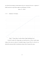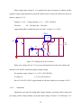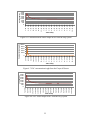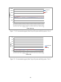
1
DEVELOPMENT OF A COST EFFECTIVE WIRELESS SENSOR SYSTEM
FOR INDOOR AIR QUALITY MONITORING APPLICATIONS
Sherin Abraham, B.Tech
Thesis Prepared for the Degree of
MASTER OF SCIENCE
UNIVERSITY OF NORTH TEXAS
May 2014
APPROVED:
Xinrong Li, Major Professor
Yan Wan, Committee Member
Kamesh Namuduri, Committee Member
Shengli Fu, Chair of the Department of
Electrical Engineering
Costas Tsatoulis, Dean of College of
Engineering
Mark Wardell, Dean of the Toulouse Graduate
School
Abraham, Sherin. Development of a Cost Effective Wireless Sensor System for Indoor Air
Quality Monitoring Applications. Master of Science (Electrical Engineering), May 2014, 69 pp.,
7 tables, 63 figures, bibliography, 30 titles.
Poor air quality can greatly affect the public health. Research studies indicate that indoor
air can be more polluted than the outdoor air. An indoor air quality monitoring system will help
to create an awareness of the quality of air inside which will eventually help in improving it. The
objective of this research is to develop a low cost wireless sensor system for indoor air quality
monitoring. The major cost reduction of the system is achieved by using low priced sensors.
Interface circuits had to be designed to make these sensors more accurate. The system is capable
of measuring carbon dioxide, carbon monoxide, ozone, temperature, humidity and volatile
organic compounds. The prototype sensor node modules were developed. The sensor nodes were
the connected together by Zigbee network. The nodes were developed in such a way that it is
compact in size and wireless connection of sensor nodes enable to collect air quality data from
multiple locations simultaneously. The collected data was stored in a computer. We employed
linear least-square approach for the calibration of each sensor to derive a conversion formula for
converting the sensor readings to engineering units. The system was tested with different
pollutants and data collected was compared with a professional grade monitoring system for
analyzing its performance. The results indicated that the data from our system matched quite
well with the professional grade monitoring system.
Copyright 2014
by
Sherin Abraham
ii
ACKNOWLEDGEMENTS
This thesis would not have been possible without my close association with many people.
I take this opportunity to extend my sincere gratitude and appreciation to all those who made this
thesis possible.
First and foremost, I would like to extend my sincere gratitude to Dr. Xinrong Li, my
advisor for his constant support and help throughout my thesis work. His continuous
encouragement and advice has helped me to improve my ways of learning and thinking styles. I
would like to thank Dr. Yan Wan and Dr. Kamesh Namuduri for being my committee members
and guiding me in my research. I am very thankful to my department for supporting me
financially for my studies.
My heartfelt regards to my friends at University of North Texas for their presence and
support have created a better learning environment. My special words of thanks goes to my
friends Shilpa Jadhav, Riya Patil and Vardhman Sheth for they have always been around helping
me in various ways. I want to thank my lab mate, Ferdoush Sheikh for his ideas and
observations.
My parents and sister have always been my greatest strength. I would not have reached this
point without their infallible love and support. I will remember with gratitude the support and
help provided by my uncle, Paul Sebastian and aunt, Nitty Pullikan. Above all I am thankful to
God Almighty for bestowing with all these goodness and good people around me. I also thank
God for giving me the strength to tide through the difficult times and overcome the hurdles in my
path.
iii
TABLE OF CONTENTS
Page
ACKNOWLEDGEMENTS ........................................................................................................... iii
CHAPTER 1. INTRODUCTION ................................................................................................... 1
1.1
Motivation and Background ................................................................................... 1
1.2
Objectives of the Research...................................................................................... 2
1.3
Contribution to the Research .................................................................................. 2
1.4
Organization of the Thesis ...................................................................................... 3
CHAPTER 2. DESCRIPTION OF THE SYSTEM: INDOOR AIR QUALITY MONITORING
SYSTEM ......................................................................................................................................... 4
CHAPTER 3. DESIGN OF INTERFACE CIRCUITS FOR SENSORS ....................................... 6
3.1
Introduction ............................................................................................................. 6
3.2
Sensor Details ......................................................................................................... 6
3.3
3.2.1
CO2 Sensor (MG811).................................................................................. 6
3.2.2
VOC Sensor (TGS 2602) ............................................................................ 8
3.2.3
Ozone Sensor (MQ131) .............................................................................. 9
3.2.4
Carbon Monoxide Sensor (MQ-7) ............................................................ 10
3.2.5
Temperature and Humidity Sensor (RTH03) ........................................... 11
Measuring Circuits ................................................................................................ 12
3.3.1
3.4
Signal Conditioning Circuit for CO2 ........................................................ 14
Heating Circuits .................................................................................................... 17
3.4.1
Heating Circuit for CO2 Sensor................................................................ 18
3.4.2
Heating Circuit for VOC Sensor ............................................................... 22
3.4.3
Heating Circuit for Ozone Sensor ............................................................. 25
3.4.4
Heating Circuit for CO Sensor .................................................................. 28
CHAPTER 4. DESIGN AND DEVELOPMENT OF SENSOR NODE MODULES.................. 35
4.1
Introduction ........................................................................................................... 35
4.2
Processing Unit ..................................................................................................... 36
4.3
Wireless Communication Module ........................................................................ 37
4.3.1
Xbee PRO S2B ......................................................................................... 37
iv
4.3.2
Xbee Shield ............................................................................................... 38
4.4
Design of Sensor Shield Type I ............................................................................ 39
4.5
Design of Sensor Shield Type II ........................................................................... 41
4.6
Implementation ..................................................................................................... 43
CHAPTER 5. NETWORK ARCHITECTURE AND DATA ACQUISITION ........................... 46
5.1
5.2
Network Architecture............................................................................................ 46
5.1.1
Operation of Communication Module ...................................................... 46
5.1.2
ZigBee Protocol ........................................................................................ 47
5.1.3
Implementation ......................................................................................... 48
Data Acquisition ................................................................................................... 49
CHAPTER 6. CALIBRATION .................................................................................................... 50
6.1
Calibration Setup .................................................................................................. 50
6.2
Experiments .......................................................................................................... 51
6.3
6.2.1
Experiment -1............................................................................................ 51
6.2.2
Experiment -2............................................................................................ 53
Modeling and Estimation ...................................................................................... 56
6.3.1
Conversion formula for the VOC Sensor.................................................. 58
6.3.2
Conversion formula for the CO Sensor .................................................... 59
CHAPTER 7. RESULTS AND ANALYSIS................................................................................ 61
7.1
7.2
Testing................................................................................................................... 61
7.1.1
Test 1......................................................................................................... 61
7.1.2
Test-2 ........................................................................................................ 63
Analysis................................................................................................................. 65
CHAPTER 8. SUMMARY AND FUTURE WORK ................................................................... 67
BIBLIOGRAPHY ......................................................................................................................... 68
v
CHAPTER 1
INTRODUCTION
1.1
Motivation and Background
Scientific evidence indicates that indoor air can be more seriously polluted than the
outdoor air. Indoor air pollution is caused by indoor as well as outdoor pollutants. The industrial
emissions and traffic exhaust are some of the sources of outdoor pollutants which can enter
inside and get trapped if the ventilation of the building is inadequate. The main sources of indoor
pollutants are cooking, smoking, cleaning, construction materials, central heating and cooling
systems and humidification devices, biological pollutants etc.[19][26]. Some of the major
pollutants are CO2, CO, VOCs, ozone, radon, dust and so on.
The US Environmental Protection Agency and its Science Advisory Board lists poor air
quality as the top five health concerns. An average person spends 90 percent of their time
indoors according to the research studies. People exposed to poor indoor air quality
environments may get sick with symptoms such as headache, eye irritation, fatigue, dry
throat, sinus congestion, dizziness, and nausea. Diagnosing sick building syndrome is difficult
since many illnesses can cause the same symptoms. Extremely high levels of some contaminants
can cause more serious illness like chronic respiratory diseases, heart disease, and lung cancer
including death [20].
Therefore, it is very essential to improve indoor air quality. Here comes the need of
building a monitoring system to detect the pollutants and its concentration as detection is the first
step towards air quality improvement.
1
1.2
Objectives of the Research
Most monitoring systems available in market are very expensive and many of them have
to be the taken to the spot of pollution to take the readings. One of the professional monitoring
systems available is Graywolf Direct Sense IQ 610 System. It is very costly as it uses very
accurate sensors. In addition it is very bulky and has to be carried to the place which has to be
monitored. Another one available is wireless IAQ profile monitor by PPM Technologies
Ltd. This system uses several sensor nodes which can measure 3 to 7 parameters, networked in
mesh topology [22]. But main problem for this system is its high price. A low cost monitoring
system is essential for making indoor air quality monitoring more popular. Using wireless
technology helps to collect data from remote areas and multiple locations simultaneously.
The aim of the research is to develop a low cost indoor air quality monitoring system which is
compact in size and capable of efficiently collecting air quality parameters from different
locations at a time. Then this data can be made available in the Internet so that the sensor node
data can be accessed by any location in the world.
1.3
Contribution to the Research
This thesis involved the development of a low cost reliable monitoring system to monitor
the indoor air quality parameters. The major cost reduction of the system is achieved by using
low cost sensors. First part was to design interface circuits to make it more accurate. Then
prototype sensor node modules were developed. Six air quality parameters can be measured by
the system developed. Then, linear least-square approach was employed for the calibration of
each of these sensors to derive a conversion formula for converting the sensor readings to
engineering units. A wireless sensor network was developed to acquire data from the individual
2
sensor nodes and store the data to a PC. Finally, the system was tested with different pollutants
to analyze its performance.
1.4
Organization of the Thesis
The whole idea of the indoor air quality monitoring system is explained in Chapter 2.
First part in building the system is the design of sensor node modules. The sensors and their
interface circuits form some of the major components of the sensor node. The details of each
sensor, its working, design and simulation of conditioning circuits are explained in Chapter 3.
The parts of sensor node module, its selection, design of sensor shields and module
implementation are discussed in the 4th chapter. In 5th chapter the network architecture,
communication protocol, building of the network and how the data is collected are detailed. The
sensors did not have any formula for converting their output to gas concentration units.
In addition, these sensors may not be very precise. Hence, they had to be calibrated. The 6th
chapter deals with calibration, estimation and derivation of conversion formula. Then the system
is tested. The experiments done with the system, the results obtained and observations are
discussed in Chapter 7. Finally, the summary and future work is given in the Chapter 8.
3
CHAPTER 2
DESCRIPTION OF THE SYSTEM: INDOOR AIR QUALITY MONITORING SYSTEM
The main components of the system are sensor nodes, base station, and server. The
sensor nodes collect the indoor air quality (IAQ) information from different locations inside the
building and this data is sent to the base station. The base station forwards it to a server. Then, it
can be made available in the internet which can be accessed by web clients.
Firstly, a sensor node has to be designed considering several factors like cost, size, and
power consumption. The parameters that can be measured by the system are ozone, carbon
dioxide, carbon monoxide, temperature and humidity. The cost reduction is achieved by using
inexpensive sensors. Hence, these sensors had to be conditioned and calibrated. The Arduino
Uno is used as the processing unit and Xbee module is communication unit for the sensor node.
The sensor nodes can be placed at several locations for the collection of IAQ data simultaneously
from multiple locations. The nodes are connected together by a Zigbee network. The coordinator
or base station is an Arduino board with Xbee module. The coordinator is connected to a
computer using a USB cable to store the IAQ data in the computer. The router node can help in
routing the data and coordinator is in charge of the whole network. These details are seen in
detail in Chapter 5. The data can then be put in the Web server. The development of the Web
portal is not covered in this thesis. The block diagram of the system is given in Figure 2.1.
4
Internet
Computer
(Web Clients)
IAQ data
Computer
Computer
(Server)
(Web Clients)
Base Station
(Coordinator)
Sensor Node
Sensor Node
(Router)
(Router)
Sensor Node
Sensor Node
Sensor Node
Sensor Node
(End Device)
(End Device)
(End Device)
(End Device)
Figure 2.1.Block diagram of the indoor air quality monitoring system.
5
CHAPTER 3
DESIGN OF INTERFACE CIRCUITS FOR SENSORS
3.1
Introduction
The sensors we have used in our system are carbon dioxide, carbon monoxide, ozone,
volatile organic compounds (VOC) and temperature-humidity sensors. The gas sensors belong to
the category of chemical and semiconductor type sensors. These sensors require heating and
signal conditioning circuits for proper functioning.
The design, simulation and testing of the heating and conditioning circuits for each sensor
is detailed in this chapter. The design and simulations of the circuits was performed using the
software, Cadence PSpice ver. 16.6. Cadence PSpice is industry-proven advanced circuit
simulation software for mixed or analog signal circuits. It is capable of simulating designs from
power supplies to high-frequency systems to simpler IC designs. After doing the simulations the
circuits were tested by setting them on the bread board. Tests were conducted using a DC power
supply and Agilent multimeter.
Before going to the circuit design and testing the working principle and characteristics of
each sensor are explained.
3.2
Sensor Details
3.2.1
CO2 Sensor (MG811)
MG811 sensor is a chemical sensor. The range of carbon dioxide it can detect is 350-
10000 ppm. It works using the solid electrolyte cell principle. When the sensor is exposed to
carbon dioxide gas, chemical reactions occur in the cell producing an electromotive force. The
6
surface temperature of the sensor needs to be high enough for these reactions to take place.
Hence, a separate heating circuit is used to heat the sensor to the required temperature [1].
The pins of the sensor along with its connection diagram are shown in Figure 3.1. The H
pins correspond to the pins of the heating coil. The output is obtained from A and B. The
specifications of the sensor are given in the Table 3.1.
Table 3.1. Specifications of the CO2 sensor.
Parameter
Value
Output Voltage
100mV-600mV (400-10000ppmCO2)
Heating Resistor
30.0 ± 5% Ω
Heating Voltage
Heating Current
Heating Power
Operating Temperature
Storage Temperature
Figure 3.1. (a) CO2 Sensor.
6 ±0.1 V (AC or DC )
~200 mA
~1200 mW
-20 to 50 C
-20 to +70 C
(b) Pins and connection of the CO2 sensor [1].
The Arduino has a 6 channel 10 bit inbuilt ADC. Hence input voltages from 0V -5V
correspond to 0-1023 integer values .So the resolution is 4.9 mV per unit integer value [9]. As
the output voltage of the sensor is very low (100mV -600mV), it needs to be amplified in order
to improve the accuracy of measurements. It also requires an external heating supply as its power
requirements cannot be satisfied by the microcontroller. Therefore, it becomes essential to
develop a signal conditioning and heating circuit for this sensor.
7
3.2.2
VOC Sensor (TGS 2602)
TGS 2602 is a heating semiconductor type sensor. It consists of a sensing layer composed
of metal oxide material like tin dioxide or zinc dioxide. This sensing layer is formed on the
alumina substrate of the sensing chip along with an integrated heater. The heater requires a warm
up time as the semiconducting oxides are sensitive to vapor and other chemicals [5] [28]. The
conductivity of sensor increases when it is exposed to detectable gases. The change in
conductivity produces an output signal corresponding to the gas concentration [4].
TGS 2602 is highly sensitive to low concentrations of gases like ammonia, hydrogen
sulfide and toluene. Its detection range is 1-30 ppm. Low power consumption, long life, simple
circuit, small size and high sensitivity to odorous gases are some of the advantages of this sensor.
Figure 3.2. (a) VOC sensor.
(b) Pin diagram and connections of the sensor [4].
The VOC sensor has four pins as shown in the Figure 3.2. Pin 1 and Pin 4 are the heater
pins and Pin 3 corresponds to sensor’s positive electrode and Pin 2 corresponds to its negative
electrode. As shown in the connection diagram the heater pins has to be provided a voltage of
VH.A circuit voltage of VC has to be applied to measure the output voltage across the adjustable
resistor RL .
8
Table 3.2. Specifications of VOC sensor.
Parameter
Value
Circuit Voltage (VC)
5.0 ± 0.2 V AC/DC
Heater Voltage(VH)
5.0 ± 0.2 V DC
Heater Current
56 ± 5 mA
Heater resistance(RH)
55 Ω at room temperature
Heater Power Consumption
280 mW
Detection Range
1-30 ppm
Conditioning Period
7 days
Sensor resistance(RS – normal conditions)
10k Ω -100k Ω
Since the output of sensor is in the range of 0V to 5 V, special amplification circuits are
not required. The load resistance RL was selected as 3.3Kohms as it gave a good range of output
voltage. Separate heating circuit is designed for the betterment of the sensor performance.
3.2.3
Ozone Sensor (MQ131)
MQ131 gas sensor is a heating semiconductor type sensor. The sensitive material in this
sensor is tin oxide. This sensor’s composition and working principle is the same as explained for
VOC sensor.
It is highly sensitive to ozone. It is also sensitive to gases like chlorine and nitrogen
dioxide. Long life, low cost, wide range of sensitivity of ozone is some features of this
sensor [6].
Table 3.3. Sensor specifications.
Parameter
Circuit Voltage (VC)
Heater Voltage(VH)
Heater resistance (RH)
Heater Power Consumption
Value
≤ 24 V DC
5.0 ± 0.2 V AC/DC
31 ± 3 Ω (Room Temperature)
≤ 900 mW
VC = 5.0 ± 0.1 V
VH = 5.0 ± 0.1 V
10-1000 ppb
More than 48 hours
50k Ω -500k Ω (in 100 ppb of Ozone)
Standard test circuit conditions
Detection Range
Conditioning Period
Sensor resistance
9
Figure 3.3(a) Ozone sensor.
(b) Pin diagram [6].
(c) Connection diagram [6].
The ozone sensor is a six pin sensor. The Pins A and B are used to fetch signals and H
pins are used for heating the sensor. For the measurement of sensor a loop voltage VC and heater
voltage VH has to be applied to the sensor pins as shown in the connection diagram in
Figure 3.3. When the sensor reaches the required temperature output is measured across the
adjustable load resistor RL. The load resistor RL is connected in series with the sensor.
The value is of this resistor is chosen in such a way to obtain a good range of output
voltage. We have taken its value as 10kohms. For meeting the heating power requirements of the
sensor, a heating circuit has to be designed. The specifications of the sensor are given in
Table 3.3.
3.2.4
Carbon Monoxide Sensor (MQ-7)
Carbon monoxide sensor is also a heating semiconductor sensor similar to VOC and
ozone sensors although its heating requirements is slightly different from them. The working
principle and composition of the semiconductor type sensor are explained in section 3.2.2.
It is highly sensitive to carbon monoxide and has long stable life.
10
Figure 3.4 (a) CO sensor.
(b) Connection and pin diagram [7].
Table 3.4. Sensor Specifications.
Parameter
Circuit Voltage (VC)
Heater Voltage(High-VHH)
Heater Voltage(Low-VHL)
Heater time(High)
Heater time(Low)
Heater resistance (RH)
Heater Power Consumption
Standard working conditions
Detection Range
Conditioning Period
Sensor resistance
Value
5.0 ± 0.1 V AC/DC
5.0 ± 0.1 V AC/DC
1.4 ± 0.1 V AC/DC
60 ± 1 seconds
90 ± 1 seconds
33 ± 5 % Ω (Room Temperature)
~ 350 mW
VC = 5.0 ± 0.1 V ,VHH = 5.0 ± 0.1 V , VHL =1.4 ± 0.1 V
RL=10k Ω ,Temperature -20 ±2% ,Humidity 65% ±5%
20-2000 ppm CO
More than 48 hours
2k Ω -20k Ω (in 100 ppm of CO)
The connection and pin diagram is as shown in Figure 3.4. For standard working
condition the circuit voltage VC is 5 ± 0.1 V .For heating the sensor a high and low voltage has
to provided alternatively. After applying a high voltage of 5 ± 0.1 V for 60 seconds a low
voltage of 1.4 ± 0.1 V has to be provided for 90 seconds. The output signal measurements is
made across resistor RL after every heating cycle .i.e., 2.5 minutes from high voltage to low
voltage. The value of RL for standard working condition is 10kohms as per the datasheet [7].
3.2.5
Temperature and Humidity Sensor (RTH03)
RTH03 is a digital sensor. It is very compact with low power consumption and long term
11
stability. For collecting the data from the sensor the microcontroller has to send a start signal to
the sensor. The sensor then changes its status from stand-by to running and sends a 40 bit data
indicating the temperature and relative humidity. After that the sensor changes it status to
standby mode and remains in this mode till it gets another start signal from the microcontroller.
Figure 3.5(a) RTH03.
(b) Connection diagram [8].
Table 3.5. Specifications
Parameter
Power Supply
Current Supply
Sensing Element
Operating Range
Accuracy
Sensitivity
Data collection Period
Value
3.3 – 6V DC
1-1.5 mA
Polymer humidity capacitor
Humidity
0-100%RH
Temperature -40 – 80C
Humidity
± 2%RH
Temperature ± 0.5C
Humidity
0.1%RH
Temperature 0.1C
2 seconds
As this sensor is temperature compensated and calibrated, the humidity and temperature
measurements can be easily taken. It can be hooked up as in the connection diagram as given in
Figure 3.5. for taking the measurements. The detailed specifications are given in Table 3.5.
3.3
Measuring Circuits
We use Arduino as the processing unit. The Arduino’s analog pin can read values from
0V -5V.Hence the output voltages of the sensors are adjusted to be in this range for getting
12
accurate measurements. The output of carbon dioxide sensor was 100-600 mV.Hence
amplification and filtering circuits were designed for this sensor. For the other gas sensors output
can be adjusted by selecting appropriate resistance. The values of resistances selected are given
in the section 3.2 along with sensor details.
The signal conditioning circuit of the carbon dioxide sensor consists of amplification and
filter circuit. Operational amplifier MCP6001 was chosen as the amplifier. It supports rail to rail
input and output voltage operation .It has gain bandwidth product of 1MHz and operates for
single supply voltage ranging from 1.8V to 6V[2].All these features make it very apt for our
purpose. A low pass filter is used to filter the high frequency noise. A capacitor of 100 nF was
used as the filter.
The voltage source V2 in the conditioning circuit as shown in Figure 3.6. represents the
sensor’s output voltage. The resistors R1 and R2 determine the gain of the amplifier. The
capacitor C1 acts as the low pass filter.
V1
5Vdc
U1
3
V2
1
Vin
2
700mVdc
0
+
5
Vout
-
4
MCP6001
R3
0
1k
R1
6.8k C1
100nF
1k
R2
0
Figure 3.6. Signal conditioning circuit for CO2 sensor.
13
3.3.1
3.3.1.1
Signal Conditioning Circuit for CO2
Design
Gain of the amplifier
The positive power supply voltage of 5V and the negative supply voltage of 0V is given
to the Op-amp. As MCP6001 can produce rail to rail output an output voltage of range 0 to 5V
can be obtained. The required gain to amplify the maximum output voltage of the sensor to the
saturation voltage of the Op-amp is,
Gain (max) = 5000mV/600mV = 8.33
The actual gain for the amplification is taken lesser than the maximum gain.
Hence, Gain = 7.8
The gain of MCP6001 is given by the equation,
G = 1+ R1/R2.
To obtain the gain of 7.8 we set
R1 = 6.8 k ohms and R2 =1 k ohm.
Cut-off frequency of the filter
Arduino Uno takes 100us to read an analog input. Hence the maximum sampling
frequency possible is 10kHz.According to Nyquist Sampling rate,
Sampling frequency (max) >=2*Signal frequency
i.e.,
Signal frequency <= Sampling frequency/2 = 5kHz.
Hence the cut off frequency of filter should be less than 5 kHz. A cut-off frequency of
approximately 200 Hz can be obtained by using a 100nF capacitor. A frequency of this range
14
was selected as the change in carbon dioxide in the air is expected to be slow. A capacitor of
100nF is used as a low pass filter to obtain a cut-off frequency of 210 Hz.
Hence, C1 = 100 nF.
3.3.1.2
Simulation - DC Analysis
Figure 3.7. Input voltage vs. output voltage of signal conditioning circuit.
For the DC analysis DC voltage input was varied from 0mV to 700 mV and the output
voltage of the circuit was observed. An amplified output of range 4700 mV to 800 mV was
obtained for maximum (600mV) and minimum voltage (100 mV) output of the sensor.
15
3.3.1.3
AC Analysis -Frequency Analysis
Figure 3.8. Frequency response of the filter.
The frequency response was obtained by giving an input signal of magnitude 600 mV
with frequency varying from 10Hz to 30kHz.The Gain of Op-amp in Decibels is,
G =20 log (Vo/Vin)
Since the input signal magnitude given is Vin =600mV the output is Vo=4700mV.The
the gain is G=20 log (4700/600) = 17.87 Db.
From the Figure 3.8.it is observed that the same gain is obtained. The cut-off frequency
of filter is found to be 210 Hz. Hence the filter passes signals with frequency lesser than 210 Hz
and attenuates signals greater than 210 Hz.
3.3.1.4
Experiments and Tests
The tests were conducted using Agilent multimeter and a power source. DC voltage was
16
applied to the conditioning circuit using a power source. The amplified voltage observed from
the multimeter was found to match with the simulated results. The Figure 3.9. shows that the
circuit produced an output of 4.45V when an input voltage of 600 mV was given.
Figure 3.9. Experimental Setup for Conditioning Circuit.
3.4
Heating Circuits
All the gas sensors have to be heated to a particular temperature for its working. Each of
them requires specific heating voltage requirements. Carbon dioxide sensor required 6V
regulated heating voltage while ozone and VOC sensor required 5V. Carbon monoxide sensor
required 2 voltage levels which has to be switched alternately after certain time periods.
LM317T was selected as the voltage regulator for obtaining constant voltage levels.
LM317T is a three terminal positive adjustable regulator which can give a regulated output
between 1.2V to 37V. It is capable of providing an output current of more than 1.5 A [3].
17
Figure 3.10. Pins and connection diagram [3].
The pins of the regulator and the circuit for general applications are given in Figure 3.10.
The resistors R1 and R2 determine the voltage output of the regulator. The capacitor Co is added
to improve the transient response and Ci is used when the regulator is located far from the power
supply filter.
The voltage output of the regulator is given by the equation,
Vo = 1.25 (1+R2/ R1) + Iadj R2
[3].
Since Iadj is lesser than 100 uA the term Iadj R2 can be neglected.
Then,
3.4.1
3.4.1.1
Vo ≅ 1.25(1+R2/R1).
Heating Circuit for CO2 Sensor
Design
The heating circuit of the sensor requires a heating voltage of 6±0.1 V and current of
200mA as given in Table 3.1.The heating circuit is shown in Figure 3.11.R3 is the sensor’s
heating resistance at room temperature.
The output of the regulator is Vo = 1.25(1+R2/R1)
The value of the resistors is obtained by equating the output voltage equation to 6V.
6V = 1.25(1+R2/R1)
R2/R1 = 3.8
18
Taking R1 =180 ohms, R2 =684 ohms. R2 is approximated to a standard resistance value
680 ohms.
Therefore, R2=680 and R1=180.
This gives Vo = 5.972 V.
U1
LM317K
2
Iin
V1
OUT
3
Iout
1
15Vdc
IN
ADJ
Vin
C2
0.1u
R1
C1
1u
Vout
R3
30
Heating
R2
680
resistor
180
0
Figure 3.11. Heating circuit for CO2 sensor.
3.4.1.2
Simulations
From the simulation graph shown in the figure 3.12., it was observed that a constant
output voltage of 6V could be achieved for the input voltages between 8 V to 15V. Figure 3.13.
shows that the heating circuit takes a current of 207 mA.
19
Figure 3.12. Output voltage vs. input voltage of the heating circuit.
Figure 3.13. Input voltage vs. input current.
20
3.4.1.3
Experiments and Tests
The circuit was tested using a DC power supply and Agilent multimeter .When the input
voltage was varied from 8V to 15V, a constant output voltage of 5.94V was attained. The heating
resistor of the sensor was connected as the load. As shown in the Figure 3.14. the circuit was
given an input of 15V to produce an output of 5.94V. It is a little lesser than the simulated
output. This could be due to the losses in the circuit.
The current intake was observed to be 130 mA. The current consumption was lesser than
the simulated current as the resistance of the heater resistor increased due to the temperature rise.
The sensor heater resistance was measured using the multimeter. It was measured to be 45 ohms
when it got heated to the required temperature. It was increased from 30 ohms to 45 ohms.
Figure 3.14. Experimental setup for heating circuit.
21
3.4.2
Heating Circuit for VOC Sensor
3.4.2.1
Design
The heating resistor of the sensor requires a voltage of 5 ± 0.2 V and takes a current of
approximately 56 mA. The resistor R3 in the Figure 3.15. represents the heating resistance of the
VOC sensor at room temperature. The values for resistors R1, R2 and R4 are chosen using the
output equation of the regulator given as,
Vo = 1.25 ( 1+ (R2+R4)/R1)
Putting Vo=5V,
5 = 1.25(1+ (R2+R4)/R1)
Taking R1 = 240 ohms, R2+R4 = 720 ohms
Approximating the resistance values to available standard resistors,
R1=240 ohms, R2=680 ohms and R4=36ohms
U1
LM317K
2
Iin
V1
OUT
C2
0.1u
3
R1
1
15Vdc
IN
ADJ
Vin
R2
680
240
Iout
C1
1u
Vout
R3
59
R4
36
0
Figure 3.15. Heating circuit for VOC sensor.
3.4.2.2
Simulations
The graphs of input voltage vs. output voltage and input current vs. output voltage were
plotted in Cadence PSpice. In the Figure 3.16., it was observed that a constant voltage of 5.01V
22
was obtained when input voltage was varied from 7V to 15V.
Figure 3.16. Input voltage vs. output voltage.
From the graph in Figure 3.17. the current consumption was observed to be a constant of
90.1 mA when input voltage was varied from 7V to 15V.
23
Figure 3.17.Input current vs. input voltage.
3.4.2.3
Experiments and Tests
The circuit was tested using a dc power supply and Agilent multimeter. A constant output
voltage of 4.99V could be obtained when the input voltage was varied from 7V to 15V. The
heating resistor of the sensor was connected as the load. As shown in the Figure 3.18. the circuit
was given an input of 15V to produce an output of 4.99V. The difference of .02V with the
simulated voltage could be the losses in the circuit.
The input current of the circuit was measured to be 63.16mA. The current consumption
was lesser than the simulated current as the resistance of the heater resistor increases when
temperature rises. To ensure the increase in resistance the heater resistance of the sensor was
measured. It was measured to be 79 ohms under operating conditions.
24
Figure 3.18. Experimental setup for heating circuit.
3.4.3
3.4.3.1
Heating Circuit for Ozone Sensor
Design
The heating requirements for ozone sensor are 5V and 180 mA approximately. The
regulator has a maximum current capacity of 1.5A. This sensor needs the same voltage as that for
VOC Sensor. Hence the heating circuit design was similar to that of the VOC sensor. Therefore,
R1=240 ohms, R2=680 ohms and R4=36 ohms. The design circuit with the heating resistor of
ozone sensor as load (R3) is shown in Figure 3.19.
U1
LM317K
2
Iin
V1
OUT
C2
0.1u
3
R1
1
15Vdc
IN
ADJ
Vin
R2
680
240
Iout
C1
1u
R4
36
0
Figure 3.19. Heating circuit for ozone sensor.
25
Vout
R3
31
3.4.3.2
Simulations
The graphs of input voltage vs. output voltage and input voltage vs. input current were
plotted in Cadence PSpice. In the Figure 3.20., it was observed that a constant voltage of 5.01 V
was obtained when input voltage was varied from 7V to 15V.
Figure 3.20. Input voltage vs. output voltage.
From the graph in Figure 3.21., the current consumption was observed to be a constant of
166.6 mA when input voltage was varied from 7V to 15V.
26
Figure 3.21. Input voltage vs. input current.
3.4.3.3
Experiments and Tests
The power is provided using a power supply and measurements was taken using a
multimeter. A constant output voltage of 4.99V could be obtained when the input voltage was
varied from 7V to 15V. The heating resistor of the sensor was connected as the load. As shown
in the Figure 3.22., the circuit was given an input of 15V to produce an output of 4.99V .The
difference of .02V with the simulated voltage could be the losses in the circuit.
The input current of the circuit was measured to be 165 mA. The current consumption
almost the same as the simulated result obtained.
27
Figure 3.22. Experimental setup.
3.4.4
3.4.4.1
Heating Circuit for CO Sensor
Design
The CO sensor requires a high voltage and low voltage to be provided alternately for its
heating. After applying a high voltage of 5 ± 0.1 V for 60 seconds a low voltage of 1.4 ± 0.1 V
has to be provided for 90 seconds. A transistor is used in combination with the regulator for
switching between the two regulated voltages. The transistor used is 2N2222.This transistor is a
NPN bipolar junction transistor which can be used for medium and low power application with
high switching speeds.
In the circuit in Figure 3.23., V1 represents the adapter voltage i.e., the input for the
circuit. The resistors R1, R2, R3 and R4 are used for determining output voltage of regulator.
The resistor R7 is the heating resistor. The voltage source V2 represents the control voltage of
transistor and R5 represents the base resistance.
28
When a high control voltage (5 V) is applied to the base of transistor it conducts and the
regulator voltage output depends on resistor R1 and R4. Hence resistors R1 and R4 are chosen to
obtain a voltage of 1.4 V.
Putting Vo =1.4V, Voltage equation is, 1.4 = 1.25(1+ (R4/R1))
Therefore,
R1 = 240 ohms, R4 = 28.8 ohms
Approximating R4 to standard resistor value, R4= 30 ohms, Vo =1.406 V.
U1
LM317K
2
Iin
IN
OUT
ADJ
Vin
V1
Vout
R1
1
15Vdc
3
C2
0.1u
R4
30
V2
5Vdc
R5
R2
680
240
C1
1u
R7
33
Q1
2N2222
470
R3
30
R6
2k
0
Figure 3.23. Heating circuit for CO sensor.
When a low voltage (0V to 0.7V) is given to the transistor base it does not conduct and
thus the R1, R2 and R3 controls the regulator output voltage.
The regulator output voltage is, Vo =1.25(1+ (R2+R3)/R1))
To obtain 5V,
5 =1.25(1+(R2+R3)/R1))
Since R1=240, R3=30,R2 is approximated to 680 ohms which gives an output of 4.91 V.
3.4.4.2
Simulations
Simulations were done by keeping input voltage constant, varying the control voltage and
by keeping control voltage constant, varying the input voltage. In Figure 3.4.2 and Figure 3.4.3
29
the voltage output and current intake is plotted for control voltage ranging from 0 to 5V keeping
input voltage constant whereas in Figure 3.24. and Figure 3.25. the output voltage and input
current is plotted for input voltage of range 7V to 15V keeping control voltage constant.
From the Figure 3.24., it is observed that a voltage of 4.97V is obtained when control
voltage is LOW (0 to 0.6V) and a voltage of around 1.42V is obtained when the control voltage
is HIGH.
As in Figure 3.25. the current intake is observed to be 153 mA when control voltage is
LOW and around 45 mA when control voltage is HIGH with the input voltage (Vin) 15V.
Figure 3.24. Output voltage vs. control voltage (V2) ,Vin=15V.
30
Figure 3.25. Input current vs. control voltage (V2), Vin=15V.
Figure 3.26. shows that a regulated voltage of 4.98 V is obtained when input voltage is
varied from 7V to 15V when control voltage is kept at 0V.
31
Figure 3.26. Input voltage (Vin) vs. output voltage (Vout), V2=0V.
It is observed that an output voltage of 1.42 V could be obtained when the input voltage
is varied from 7V to 15V keeping the control voltage at 5V.
Figure 3.27. Input voltage (Vin) vs. output voltage (Vout), V2=5V.
3.4.4.3
Experiments
Two power supplies were provided, one for the control voltage and the other for the input
voltage. A constant output voltage of 4.92V was obtained when the input voltage was varied
from 7V to 15V at control voltage set as 0.42 V as shown in the Figure 3.28.
32
Figure 3.28. Experimental setup 1.
Figure 3.29. Experimental setup 2.
Similarly regulated voltage of 1.42 V was obtained for input voltages of range 7V to 15V
when the control voltage was set as 5V as in Figure 3.29.
33
The control voltage was varied from 0V-5V keeping the input voltage of 15V.The output
voltage remained at 1.42 V when control voltage was varies from 0 to 0.7V.It changed to 4.92V
when the control voltage was above 1.0V.
34
CHAPTER 4
DESIGN AND DEVELOPMENT OF SENSOR NODE MODULES
4.1
Introduction
The sensor node module we developed is equipped with multiple sensors, a processing
unit, a wireless communication module for receiving and transmitting various sensed signals and
commands and an adapter for power supply. The processing unit is Arduino Uno, a
microcontroller board based on Atmega328. Wireless communication is achieved by using the
Xbee module. For placing multiple sensors with their conditioning circuits Sensor Shields were
designed.
The side view of the sensor node is shown in the Figure 4.1. The main components of the
node are Arduino board, Xbee shield, Xbee and the sensor shield. The Xbee module and sensor
shield are placed on the Xbee shield. This Xbee shield is mounted on top of the Arduino board.
Xbee
Sensor Shield
Xbee Shield
Arduino Uno Board
Figure 4.1. Block diagram of sensor node module.
Several factors like cost, power consumption, space utilization was considered for the
design of the module. We have put the sensors in two separate sensor shields so as to make the
sensor node compact and handy. Hence two types of sensor shields were designed which had
different sensors. The temperature-humidity Sensor was placed in both the shields to observe if
the output of gas sensors depended on the humidity and temperature variations. We will look into
the details of each part, their selection, design and the final implementation of the sensor node in
the following sections.
35
4.2
Processing Unit
The core of our platform is selected as Arduino UNO, a single board microcontroller. The
open source hardware and software, low cost, easy to use programming and programming
environment make it popular among the other microcontroller platforms.
Arduino UNO is the latest version of basic Arduino USB boards.The board contains a
16MHz ceramic resonator, a USB connection, a power jack, an ICSP header, and a reset button.It
also has 14 Digital I/O pins of which 6 is capable of providing PWM output and 6 analog input
pins. The serial communication is available on digital pins 0 (RX) and 1 (TX).The power pins
are Vin,5V,3V3,Gnd and IOREF. Arduino can be powered through USB or the power jack using
an AC-DC adapter or battery.If it is powered by both the board automatically selects one of it[9].
Table 4.1. Specifications.
Parameter
Operating Voltage
Input Voltage
Current per I/O Pin
Current for 3.3V pin
Clock Speed
Memory (ATmega328)
Value
5V DC
6-20V( Maximum limits)
7-12V (Recommended)
40 mA
50 mA
16 MHz
Flash Memory - 32 KB , 0.5 KB used by bootloader
SRAM - 2 KB
EEPROM - 1 KB
Figure 4.2. Arduino Uno R3 board [9].
36
The microcontroller in Arduino UNO is Atmega328. It is preprogrammed with a
bootloader which helps in uploading the programs into the microcontroller memory without the
need of an external device programmer. Atmega328 belongs to Atmel 8-bit microcontroller
family. It has advanced RISC architecture. Its features include 32KB flash memory with readwhile-write capabilities, 1KB EEPROM, 2KB SRAM, 23 general purpose I/O lines, 32 general
purpose working registers, three flexible timer/counters with compare modes, internal and
external interrupts,serial programmable USART, a byte-oriented 2-wire serial interface, SPI
serial port, 6-channel 10-bit A/D converter, programmable watchdog timer with internal
oscillator, and five software selectable power saving modes.
Arduino is programmed using the Arduino programming language (based on Wiring) and
the Arduino development environment (based on Processing). Its features are briefed in the
Table 4.1.
4.3
Wireless Communication Module
4.3.1
Xbee PRO S2B
We have used Xbee module for wireless communication as they are small, cost effective
radios which enable low power and low bandwidth simple wireless communication. Xbee is a
wireless microcontroller made by Digi International. It has 20 pins of which 11 are digital I/O
pins and 4 are analog pins. Xbee PRO series 2 is used as it consumes lesser power and gives
better range than Xbee Series 1. It uses a frequency of 2.2 GHz [10].The communication
protocol used is Zigbee. The details on Zigbee protocol will be covered in the next chapter. The
Figure 4.4. shows the Xbee PRO S2B module. More features of Xbee are listed in the Table 4.2.
37
Table 4.2. Features of Xbee PRO S2B.
Parameter
Operating Voltage
Operating Current (Transmission)
Operating Current (Reception)
Indoor Range
RF Data Rate
Receiver Sensitivity
Network Protocol
4.3.2
Value
2.6V-3.4 V DC
205mA, up to 220 mA
47 mA, up to 62 mA
Up to 300 ft. (90 m)
250,000 bps
-102 dBm
ZigBee
Xbee Shield
An Xbee shield is used to connect Xbee to the Arduino board. The Shield makes Xbee
convenient to use as it can be directly plugged into the Arduino without the need of any other
connection. It makes the module compact and easy to use. The Xbee shield provides regulated
voltage of 3.3V for the operation of Xbee.
The Xbee shield has two jumpers .The serial communication between Xbee and computer
via the USB cable is enabled by putting the jumper in the USB position .For the Xbee to
communicate to the Arduino the jumper has to be put in Xbee position. The shield covers 8
digital pins and 6 analog pins of the Arduino. The female pin headers on the shield help to use all
the pins except the digital pins 0 and 1 which is used by Xbee. The Xbee shield we have used is
shown in Figure 4.3.
Figure 4.3. Xbee shield.
Figure 4.4. Xbee PRO S2B.
38
4.4
Design of Sensor Shield Type I
This shield is incorporated by carbon dioxide sensor, VOC sensor and temperature-
humidity sensor along with their heating and measurement circuits. Temperature-humidity
sensor is placed away from the gas sensors in the sensor shield so that its reading doesn’t get
affected due to the heat of the gas sensors. We have used a board of size 6x4cm so as to utilize
the space efficiently. A 6 pin connector and 8 pin connector were used so that the Sensor Shield
can be mounted on top of the Arduino board containing the Xbee shield.
The circuit diagram and PCB layout of the shield was designed using the Eagle PCB
Design Software [12]. The VOC and carbon dioxide required regulated voltages of 5V and 6V
respectively for their heating. It is provided by voltage regulators U2 and U1 as shown in the
circuit diagram in Figure 4.5. The output signal of carbon dioxide sensor is conditioned using the
operational amplifier MCP6001. The measuring circuits of all the sensors require 5V. It is taken
from the voltage regulator U2. The power supply and ground connections are taken from the
Arduino using a jumper JP1.The output pin of CO2 and VOC sensor is connected to the analog
pin A0 and A1 through the 6 pin connector JP2 and the digital output of temperature-humidity
sensor is connected to the digital pin 2 of Arduino via JP3 connector. The shield can be directly
plugged into the Arduino using the connectors JP2 and JP3.
After designing the circuit diagram its PCB layout was developed. It is shown in
Figure
4.6.
39
Figure 4.5.Circuit diagram of sensor shield type I.
40
Figure 4.6. PCB layout of sensor shield type I.
4.5
Design of Sensor Shield Type II
This sensor shield comprises of carbon monoxide, ozone sensor and temperature- humidity
sensor. The shield size was same as that of the shield I and the headers were used to mount the
shield easily on the Arduino. The output of the sensors was connected to the corresponding
header pins to make it easy to use and handy.
The circuit diagram of the shield is given in Figure 4.7. The main components of the
circuit diagram are sensors, regulators, transistor and connectors. One 6 pin connector and one 8
pin connector is used. The voltage regulator U2 provides 5V regulated voltage. The regulated 5V
is used for heating ozone sensor and for the measuring circuits of all the sensors. The CO sensor
requires a constant high voltage of 5V and low voltage of 1.4V to be given alternatively. This
alternating voltage is provided by regulator U1 in combination with the transistor 2N2222. The
design details of the heating and conditioning circuits had been discussed in the previous chapter.
41
The power is obtained through the Vin pin and Gnd pins of Arduino board through the
jumper JP1.The control voltage for switching the transistor on and off is given through the digital
pin 2 through the connector JP3.The output of temperature sensor is connected to the digital pin
4 by the connector JP3 and output of the other sensors are connected to analog pin 1 and analog
pin 2 via connector JP2. The PCB design of this sensor shield is given in Figure 4.8.
Figure 4.7.Circuit diagram of sensor shield type II.
42
Figure 4.8. PCB layout of sensor shield type II.
4.6
Implementation
After the development of the sensor shield boards the parts are assembled together .As
mentioned before two types of sensor nodes were made. Each node had different power
requirements which had to be considered for selecting the adapter.
First senor node contains CO2, VOC and temperature sensor. The carbon dioxide sensor
requires 6 V of constant voltage and a current of 200 mA whereas VOC needs 5V and 56 mA.
The power taken by temperature Sensor was negligible. The Xbee PRO module draws a current
of maximum 220 mA for transmission and 62 mA for reception. It requires a supply voltage of
2.7 to 3.6 V. Hence the total current taken by the sensors and the Xbee module comes around
43
476 mA .The voltage requirements are below 9V.The recommended range for powering Arduino
is 7 to 12 volts. Hence a 9V, 1 A adapter was chosen for this sensor node.
For the implementation of the module the Xbee shield and sensor shield is placed on the
Xbee shield. This Xbee shield is mounted on top of the Arduino board as shown in the
Figure 4.9.
Figure 4.9.Type I sensor node module.
The sensors in sensor node type II are ozone, CO and temperature sensor. The ozone
sensor needs a regulated voltage of 5V and 180 mA for the heating purpose. The CO sensor
requires a constant high voltage of 5V and low voltage of 1.4V and consumes a maximum
current of 250 mA. Along with the Xbee module maximum current consumption comes around
650 mA. Hence a 9V, 1 A adapter was chosen for powering this Module.
It is implemented in a similar way as senor node I. The sensor shield and Xbee is
mounted on Xbee shield which is placed on top of the Arduino .The final implementation of the
type II sensor module is as shown Figure 4.10.
44
Figure 4.10. Type II sensor node module.
45
CHAPTER 5
NETWORK ARCHITECTURE AND DATA ACQUISITION
5.1
Network Architecture
The network we propose consists of several sensor nodes organized in ZigBee network.
One of the nodes is the ZigBee coordinator, and the others are end devices or routers. Details of
the communication protocol used, operation of communication module and how the network is
set up is discussed in this section.
5.1.1
Operation of Communication Module
As mentioned before, we have used Xbee as the communication module. Its hardware
details were explained in the previous chapter. Here we will see how it operates. Xbee module
interfaces to the host device through a logic-level asynchronous serial port. The data enters the
module UART through its D3 pin. The module has a buffer to store this data. Each data byte
consists of a start bit, 8 data bits and a stop bit .The start bit has low voltage level and stop bit has
high voltage level.
It has two serial interface protocols. One is Transparent Serial Interface (AT) and the
other is packet based Application Programming Interface (API). In AT mode the data is
transmitted to the intended receiving module without any modification. For controlling the radio
settings AT commands can be used. In API mode the data has a packet structure. It allows
addressing, parameter setting, and packet delivery feedback and may also include remote sensing
and control of analog and digital pins.
It has five modes of operation. These are: Idle, sleep, transmit, receive and command
mode [10]. Xbee module is in idle mode when it is not receiving or transmitting data. It goes to
46
transmit mode when the data in the serial buffer is ready to be packetized. When the data is
received by the Xbee it enters into receive mode. When the modules are not in use it can go to
sleep mode. Only the end devices can be in this mode. In this mode it will be in a low power
consumption state. Sleep modes allow the RF module to enter states of low power consumption
when not in use. In command mode the incoming data is interpreted as commands. This mode is
used to read or change the module parameters.
5.1.2
ZigBee Protocol
ZigBee specifies a set of high level protocols for wireless networking applications. It is
based on IEEE 802.15.4 MAC/PHY as a standard and adds a network layer above it for
advanced mesh routing capabilities. It is very suitable for home and industrial applications as it
designed for low power, low data rate and low cost applications.
ZigBee operates in radio bands 868 MHz, 915 MHz or 2.4 GHz. Data transmission rates
ranges from 20 kbps to 250 kbps. It enables good network security by using 128 bit symmetric
encryption keys [17].It supports three types of devices: coordinator, routers and end devices.
Coordinator selects the PAN ID for the network and it connects routers and end devices to the
network. Each network is defined with its unique PAN ID .Hence a coordinator is in charge of
setting up the entire network. There can be only one coordinator for a network. It should always
be powered. There can be multiple routers in a network. A router has to first join a network.
After that it can allow other devices to join the network and also helps in routing data. The router
also can never go to sleep. The end devices have to join the network for transmitting or receiving
data. It can neither route data packets nor allow other devices to join the network. It can go to
low power mode called sleep mode [10].
47
5.1.3
Implementation
One of the modules is configured as a coordinator while the others are configured as
routers. There are many ways to configure the Xbee module. We have used XCTU software
from Digi International for configuring them as it is very convenient and user friendly. However
it is compatible only for Windows platform. For programming it using this software Xbee is
mounted on the Xbee shield which is plugged on the Arduino Uno board .Then it can be
programmed through the Arduino Uno’s programming interface. XCTU has mainly four tabs:
PC Settings, Range test, Terminal and Modem configuration. The PC settings enable to select the
COM port and set the radio parameters in order to configure the port. It also has a test/Query tab
to check if the connections are made properly. Using Modem configuration tab Xbee’s
parameters can be read and changed according to how we are going to use it. It also allows us to
modify the firmware versions. The Range test is used to see how good the connection is
established between two radios. The Terminal tab allows access to the computer’s COM port
with a terminal emulation program. Using this we can test if the Xbees are talking in the way we
want [13].
For building the network, first a connection is established with Xbee module and PC
using the PC settings tab .Then modem parameters is updated. Here we have set the Xbees as a
coordinator or router according to their function and firmware was updated as the latest version.
The serial interface protocol selected is Transparent Serial Interface .The network PAN ID has to
be set the same for all modules in the network and the destination address of each module is
given in such a way to make the routers and coordinator talk to each other. A screen shot of two
instances of XCTU software is shown in Figure 5.1.It shows one Xbee configured as router and
the other one configured as coordinator.
48
Figure 5.1. XCTU software showing the configuration of Xbee Modules.
5.2
Data Acquisition
The base station or coordinator receives the data at regular intervals from the routers or
sensor nodes. Each sensor node is programmed using Arduino programming for collecting the
sensor output values. A timer is set in Arduino which start counting when the program begins
running. After each 5 minutes the data is collected.
The data of individual nodes are collected by the coordinator node which is connected to
the computer. The collected values are stored in the computer in text files. Python programming
is done to store the collected data in files. Python(x,y) ver. 2.7.3 is used. It is an engineering and
scientific development software based on python programming language, Qt graphical user
interfaces and Sypder environment, used for analyzing, visualizing and computation of data [24].
49
CHAPTER 6
CALIBRATION
6.1
Calibration Setup
The sensors we have used in our system are inexpensive sensors. Its output may not be
accurate and may depend on several factors. The datasheet of these sensors did not have
conversion formulae to convert the output voltage to gas concentration units. Hence it was
necessary for these sensors to be calibrated.
For the calibration of the gas sensors it required special chamber for maintaining the gas
concentration at fixed levels, a source for generating the gas and a reference instrument for
measuring the actual gas concentration [14].The appropriate devices for calibration were not
available in the engineering laboratory nor any other laboratory on campus .Considering the cost
factors for buying these equipment we decided to test these sensors in a container and the test
gases were obtained from common sources. The container used was of size 24x13.1x16.8 inches
manufactured by Hefty. The Graywolf DirectSense IAQ 610 monitoring system was used as a
standard measuring device. It is a professional grade air quality monitoring system. It comes in a
kit which includes a tablet PC, a probe, USB cable for connecting the probe to the PC, a tripod
stand for the probe and an AC adapter. The probe contains very accurate sensors which capable
of detecting TVOC, CO2, CO, ozone, temperature, %RH, and dew point .It has option for adding
additional parameters if necessary. The tablet has software called WolfSense PC for collecting,
graphing and storing the sensed data [15].
The collected data from our system was compared with the Graywolf Sensor data and
output equation for each sensor was modeled.
50
6.2
Experiments
Several experiments were conducted for analyzing the behaviour of the output of sensors.
Initially our system and Graywolf System were kept at normal conditions and readings were
taken for about a week. Another experiment was conducted by putting both the systems inside
the test chamber and introducing a burnt paper. Readings were taken at an interval of 5 minutes.
The data collected was then plotted to study the characteristics of the sensors.
6.2.1
Experiment -1
Data was collected for different weeks from our lab at normal conditions. Our system
was kept close to the Graywolf system and readings were taken at an interval of 5 minutes.
Except for CO2, humidity and temperature all the other parameters were present in negligible
concentration. The Figure 6.1 shows the CO2 concentration from Graywolf sensor and Figure
6.2. shows the CO2 sensor output of our system. The Figures 6.3 and 6.4 shows the temperature
and humidity values collected. We can see that the carbon dioxide concentration increased from
9.00 a.m. and reached its peak at 3.00 p.m. and then gradually decreased. This variation was seen
as 10th was a Monday and the presence of people made the CO2 concentration vary. During the
2/11 , 4…
2/10 , 11…
2/10 , 6 PM
2/10 , 1 PM
Date,Time
2/10 , 8…
2/10 , 3…
2/9 , 10 PM
2/9 , 5 PM
2/9 , 12 PM
2/9 , 7 AM
2/9 , 2 AM
2/8 , 9 PM
2/8 , 4 PM
2/8 , 11…
1000
800
600
400
200
0
2/8 , 6 AM
Concentration (ppm)
previous two days (Saturday and Sunday) the concentration was almost a constant low value.
Figure 6.1. Carbon dioxide concentration in ppm from Graywolf Sensor.
51
2/11 , 4 AM
2/10 , 11 PM
2/10 , 6 PM
2/10 , 1 PM
2/10 , 8 AM
Date,Time
2/10 , 3 AM
2/9 , 10 PM
2/9 , 5 PM
2/9 , 12 PM
2/9 , 7 AM
2/9 , 2 AM
2/8 , 9 PM
2/8 , 4 PM
2/8 , 11 AM
2/8 , 6 AM
Voltage (mV)
2500
2450
2400
2350
2300
2250
2200
2150
2100
2050
2000
Figure 6.2.Carbon dioxide sensor output in mV from IAQ system.
It is observed by comparing Figures 6.1. and 6.2. that CO2 sensor voltage decreased
linearly as the CO2 concentration increased. It was also observed that the sensor output was not
dependent on humidity variations. From Figures 6.3 and 6.4. we can see that the temperature of
our system is higher and humidity is lower than the actual values. This is due to the heat
developed by the gas sensors in the module. Since the module was designed small and the
temperature-humidity sensor was put together with more than one gas sensor in a module the
reading of the temperature-humidity sensor was influenced by the heat developed in the module.
We confirmed this by hooking up a similar temperature sensor in another module and readings
were taken by keeping it far away from the other sensor nodes.
52
2/11 , 4 AM
2/10 , 11 PM
2/10 , 6 PM
2/10 , 1 PM
2/10 , 8 AM
2/10 , 3 AM
2/9 , 10 PM
2/9 , 5 PM
2/9 , 12 PM
2/9 , 7 AM
2/9 , 2 AM
2/8 , 9 PM
2/8 , 4 PM
2/8 , 11 AM
2/8 , 6 AM
Temperature(οC)
35
30
25
20
15
10
5
0
GrayWolf
IAQ
Date,Time
25
20
15
10
2/11 , 4 AM
2/10 , 11 PM
2/10 , 6 PM
2/10 , 1 PM
2/10 , 8 AM
2/10 , 3 AM
2/9 , 10 PM
2/9 , 5 PM
2/9 , 12 PM
2/9 , 7 AM
2/9 , 2 AM
2/8 , 9 PM
2/8 , 4 PM
0
IAQ
2/8 , 11 AM
5
2/8 , 6 AM
Realtive Humidity(%)
Figure 6.3.Temperature values in Celsius from Graywolf and IAQ system.
GrayWolf
Date,Time
Figure 6.4.Relative humidity in percentage from Graywolf and IAQ system.
6.2.2
Experiment -2
For the calibration VOC, CO and CO2 sensors respective gases had to be introduced. A
common source which produced all of these gases was used. A paper was burnt and was kept
near the sensors placed in the test container. We know that the incomplete combustion of a
substance produces of a mixture of carbon monoxide and carbon dioxide gas. Burning of paper is
an example of incomplete combustion. It produced CO, CO2 and VOC gases. The VOC might
53
have been produced due to the volatile matter of the burning paper. The container was kept
closed to maintain these gases for a while.
The data was collected in each 5 minute intervals by keeping the sensors along with gray
wolf sensor inside the test container. We can see from the Figure 6.5 and 6.7 that the
concentration of CO and VOC increased drastically for some time and then decreased. CO2 also
increased to 1000 ppm. Similar pattern of variation was observed for the CO2 concentration also.
Comparing the sensor output values with the concentration of the gases we observe a linear
relation for VOC and CO. For CO2 sensor the variation was similar to that found for the
Experiment -1.Figure 6.9. plots the temperature and humidity variations from the Graywolf
9:59 AM
9:09 AM
8:19 AM
7:29 AM
6:39 AM
10:49 AM
Time of day
5:49 AM
4:59 AM
4:09 AM
3:19 AM
2:29 AM
1:39 AM
12:49 AM
11:59 PM
11:09 PM
10:19 PM
9:29 PM
8:39 PM
90
80
70
60
50
40
30
20
10
0
7:49 PM
Comcentration(ppm)
sensor.
Figure 6.5. Carbon monoxide concentration in ppm from the Graywolf sensor.
54
Voltage(mV)
4500
4000
3500
3000
2500
2000
1500
1000
500
0
2:29 AM
1:39 AM
12:49 AM
11:59 PM
11:09 PM
10:19 PM
9:29 PM
Time of day
55
Figure 6.8.VOC Sensor output in mV from the IAQ System.
10:49 AM
9:59 AM
9:09 AM
8:19 AM
7:29 AM
6:39 AM
5:49 AM
4:59 AM
4:09 AM
3:19 AM
10:49 AM
9:59 AM
9:09 AM
8:19 AM
7:29 AM
6:39 AM
5:49 AM
4:59 AM
4:09 AM
3:19 AM
2:29 AM
1:39 AM
12:49 AM
11:59 PM
11:09 PM
10:19 PM
9:29 PM
8:39 PM
7:49 PM
10000
8000
6000
4000
2000
0
8:39 PM
7:49 PM
Concentration (ppb)
Voltage(mV)
10:49 AM
9:59 AM
9:09 AM
8:19 AM
7:29 AM
6:39 AM
5:49 AM
4:59 AM
4:09 AM
3:19 AM
2:29 AM
1:39 AM
12:49 AM
11:59 PM
11:09 PM
10:19 PM
9:29 PM
8:39 PM
7:49 PM
4500
4000
3500
3000
2500
2000
1500
1000
500
0
Time of day
Figure 6.6. Carbon monoxide sensor output in mV from the IAQ system.
Time of day
Figure 6.7.VOC concentration in ppb from the Graywolf Sensor.
RH%
10:49 AM
9:59 AM
9:09 AM
8:19 AM
7:29 AM
6:39 AM
Time of day
5:49 AM
4:59 AM
4:09 AM
3:19 AM
2:29 AM
1:39 AM
12:49 AM
11:59 PM
11:09 PM
10:19 PM
9:29 PM
8:39 PM
Temp(ᵒC)
7:49 PM
40
35
30
25
20
15
10
5
0
Figure 6.9. Temperature (οC) and relative humidity (%) readings from the Graywolf sensor.
6.3
Modeling and Estimation
In the above experiments, the outputs of CO, VOC sensors increased linearly as
concentration of gas is increased. For CO2 sensor voltage output decreased linearly as carbon
dioxide increased. The temperature-humidity sensors are already calibrated. They showed a
deviation in reading due to the heat dissipated within the module. It was observed from the
experiments conducted that the temperature in sensor node module-1 was higher by 4.5οC and
humidity lower by 6%.In sensor node module-2 temperature was higher by 6.5οC and humidity
lower by 7.5%. This can be corrected using a correction factor. It was observed that these gas
sensors were independent of slight temperature and humidity variations.
Therefore, a linear signal model is assumed with two unknown parameters for all the
sensors. The estimation is done using the Least Square Approach. In this method a signal model
is assumed and no probabilistic assumption is made about data. Statistical performance can’t be
assessed as no assumption of data is made. But this estimator is widely used because of its ease
of implementation [16].
56
In this estimation technique we try to minimize the squared difference between the actual
signal and the assumed signal [16]. Let the actual signal be x[n] and assumed signal be y[n].The
assumed signal may depend on several parameter. Suppose θ is the unknown parameter it is
depended on. Then least square error is given by,
2
E(θ) = ∑𝑁𝑁−1
𝑛𝑛=0 (x[n] − y[n] )
Here 𝑁𝑁 is the number of observations taken. The least square estimator is the value of θ
that minimizes E(θ) . It will be a value that makes y[n] closest to x[n].The estimation was done
in MATLAB ver.7.14 for the measurements taken from Experiment-2.
6.3.1. Conversion formula for the CO2 Sensor
The signal model for the CO2 sensor in vector form was taken as,
𝐲𝐲 = H 𝛉𝛉 , where H is the observation matrix and 𝛉𝛉 is vector parameter of dimension 2×1
a
𝛉𝛉 = � � ; here a and b are the unknown parameters.
b
H = [(5000-V) 1] [𝛉𝛉] ; V is the matrix for sensor output voltage in millivolt unit.
x[n] is the concentration measurement in ppm unit taken from the Graywolf sensor.
2
E (𝛉𝛉) = ∑𝑁𝑁−1
𝑛𝑛=0 (x[n] − y[n] )
Least square error,
= (x - H 𝛉𝛉)T (x - H 𝛉𝛉)
= xTx -2xH 𝛉𝛉 + 𝛉𝛉 T HT H 𝛉𝛉
For minimizing the least square error E (𝛉𝛉)
Putting
𝜕𝜕 E (𝛉𝛉)
𝜕𝜕𝛉𝛉
= -2HTx +2HTH 𝛉𝛉 = 0
we get, 𝛉𝛉 = (HTH)-1HTx
Solving for 𝛉𝛉 we get, a = 0.3618 and b = -472.47.
57
Hence the equation for CO2 concentration is,
y[n] = 0.3618 (5000-V[n]) - 472.47 = Estimated CO2 concentration in ppm unit.
Then voltage values were put in this equation to see if it matches with the concentration
measurement from Graywolf sensor. The Figure 6.10. plots the estimated concentration y([n])
and the concentration measurement (x[n]) taken from Graywolf system.
1200
CO2 (ppm)
1000
Graywolf
Estimated
800
600
400
0
1
10
19
28
37
46
55
64
73
82
91
100
109
118
127
136
145
154
163
172
181
200
No of Readings
Figure 6.10. Estimated CO2 concentration and the Graywolf measurement (Experiment 2).
6.3.1
Conversion formula for the VOC Sensor
The signal model for the VOC sensor was taken as,
𝐲𝐲 = H 𝛉𝛉 , where H is the observation matrix and 𝛉𝛉 is vector parameter of dimension 2×1
a
𝛉𝛉 = � � ; here a and b are the unknown parameters.
b
H = [V 1] [𝛉𝛉] ; V is the matrix for sensor output voltage ( millivolts)
x[n] is the concentration measurement in ppb unit taken from Graywolf sensor.
58
A similar procedure done for CO2 estimation was carried out for this one also. By
minimizing the least square error we get, 𝛉𝛉 = (HTH)-1HTx
Solving for 𝛉𝛉 we get,
a =1.3813 and b = – 1555.9.
Hence the conversion formula is,
y[n] =1.3813×V[n] – 1555.9 = Estimated VOC concentration in ppb unit.
Then voltage values were put in this equation to see if it matches with the concentration
measurement from Graywolf Sensor. The Figure 6.11. shows the estimated concentration (y[n])
from our system and concentration (x[n]) taken from Graywolf system.
10000
VOC (ppb)
8000
Graywolf
Estimated
6000
4000
0
1
10
19
28
37
46
55
64
73
82
91
100
109
118
127
136
145
154
163
172
181
2000
-2000
No. of Readings
Figure 6.11. Estimated VOC concentration and the Graywolf measurement (Experiment 2).
6.3.2
Conversion formula for the CO Sensor
The signal model for the CO sensor was taken the same as that of VOC sensor
𝐲𝐲 = H 𝛉𝛉
a
Vector parameter, 𝛉𝛉 = � � ; here a and b are the unknown parameters.
b
59
Observation
matrix, H = [V 1] [𝛉𝛉] ;V is the matrix for sensor output voltage (millivolts)
By minimizing the least square error the parameters are calculated.
𝛉𝛉 = (HTH)-1HTx
Solving for 𝛉𝛉 we get, a =0.017 and b = - 36.14.
Hence the equation for estimated CO concentration,
y[n] =0.017×V[n] - 36.14 = Estimated CO concentration in ppm unit.
The Figure 6.12. plots the estimated concentration (y[n])and concentration (x[n]) taken from
Graywolf system.
90
80
Graywolf
CO(ppm)
70
Estimated
60
50
40
30
10
0
-10
1
10
19
28
37
46
55
64
73
82
91
100
109
118
127
136
145
154
163
172
181
20
No. of Readings
Figure 6.12. Estimated CO concentration and the Graywolf measurement (Experiment 2).
The conversion formula for CO, CO2 and VOC sensor was modeled using the data
collected from Experiment 2.The equations modeled here were used in the tests carried out in the
next chapter for calculating the gas concentration for our system.
60
CHAPTER 7
RESULTS AND ANALYSIS
7.1
Testing
Experiments were performed with different pollutants to analyze the performance of our
system and the accuracy of the equation we modeled. The sources which produced these
pollutants were burning material for the first test and acetone based nail polish remover for the
second test. These are common pollutants that can cause poor indoor air quality.
7.1.1
Test 1
For the first test a paper was burnt for a short duration and flames were put off
immediately. Then it was put in our test chamber containing the Graywolf and IAQ system and
the chamber lid was closed. The results produced were as shown in Figures 7.1 to 7.5.
GrayWolf
5000
IAQ
4000
3000
2000
1000
0
-1000
5:59 PM
6:04 PM
6:09 PM
6:14 PM
6:19 PM
6:24 PM
6:29 PM
6:34 PM
6:39 PM
6:44 PM
6:49 PM
6:54 PM
6:59 PM
7:04 PM
7:09 PM
7:14 PM
7:19 PM
7:24 PM
7:29 PM
7:34 PM
7:39 PM
7:44 PM
7:49 PM
7:54 PM
7:59 PM
8:04 PM
8:09 PM
VOC(ppb)
6000
Time of the day
Figure 7.1.VOC concentration (ppb) from Graywolf system and IAQ system –Test 1.
61
Temperature( οC)
10
0
-10
10
0
5
5:59 PM
6:04 PM
6:09 PM
6:14 PM
6:19 PM
6:24 PM
6:29 PM
6:34 PM
6:39 PM
6:44 PM
6:49 PM
6:54 PM
6:59 PM
7:04 PM
7:09 PM
7:14 PM
7:19 PM
7:24 PM
7:29 PM
7:34 PM
7:39 PM
7:44 PM
7:49 PM
7:54 PM
7:59 PM
8:04 PM
8:09 PM
0
Time of the day
5:59 PM
6:04 PM
6:09 PM
6:14 PM
6:19 PM
6:24 PM
6:29 PM
6:34 PM
6:39 PM
6:44 PM
6:49 PM
6:54 PM
6:59 PM
7:04 PM
7:09 PM
7:14 PM
7:19 PM
7:24 PM
7:29 PM
7:34 PM
7:39 PM
7:44 PM
7:49 PM
7:54 PM
7:59 PM
8:04 PM
8:09 PM
200
Time of the day
5:59 PM
6:04 PM
6:09 PM
6:14 PM
6:19 PM
6:24 PM
6:29 PM
6:34 PM
6:39 PM
6:44 PM
6:49 PM
6:54 PM
6:59 PM
7:04 PM
7:09 PM
7:14 PM
7:19 PM
7:24 PM
7:29 PM
7:34 PM
7:39 PM
7:44 PM
7:49 PM
7:54 PM
7:59 PM
8:04 PM
8:09 PM
CO(ppm)
CO2(ppm)
1200
1000
800
Graywolf
600
IAQ
400
Figure 7.2.CO2 concentration (ppm) from Graywolf system and IAQ system –Test 1.
60
50
40
Graywolf
30
IAQ
20
Time of the day
Figure 7.3.CO concentration (ppm) from Graywolf system and IAQ system –Test 1.
30
25
20
15
Graywolf
IAQ
Figure 7.4.Temperature in Celsius from Graywolf system and IAQ system –Test 1.
62
25
20
15
Graywolf
10
IAQ
5
0
5:59 PM
6:04 PM
6:09 PM
6:14 PM
6:19 PM
6:24 PM
6:29 PM
6:34 PM
6:39 PM
6:44 PM
6:49 PM
6:54 PM
6:59 PM
7:04 PM
7:09 PM
7:14 PM
7:19 PM
7:24 PM
7:29 PM
7:34 PM
7:39 PM
7:44 PM
7:49 PM
7:54 PM
7:59 PM
8:04 PM
8:09 PM
Relative Humidity(%)
30
Time of the day
Figure 7.5.Humidity concentration (%) from Graywolf system and IAQ system –Test 1.
7.1.2
Test-2
Another test was performed to see how VOC sensors responded when it was exposed to
other types of volatile materials. For that two to three drops of nail polish remover was poured
into a piece of cotton and was placed in the test chamber with its lid closed. The nail polish
remover used was the one containing 100% acetone. The readings by both the systems are shown
in Figures 7.6 to 7.10.
7000
Graywolf
5000
IAQ
4000
3000
2000
1000
0
-1000
4:17 PM
5:07 PM
5:57 PM
6:47 PM
7:37 PM
8:27 PM
9:17 PM
10:07 PM
10:57 PM
11:47 PM
12:37 AM
1:27 AM
2:17 AM
3:07 AM
3:57 AM
4:47 AM
5:37 AM
6:27 AM
7:17 AM
8:07 AM
8:57 AM
9:47 AM
10:37 AM
VOC(ppb)
6000
Time of the day
Figure 7.6. VOC concentration (ppb) from Graywolf system and IAQ system –Test 2.
63
CO(ppm)
0
10
-10
4:17 PM
5:07 PM
5:57 PM
6:47 PM
7:37 PM
8:27 PM
9:17 PM
10:07 PM
10:57 PM
11:47 PM
12:37 AM
1:27 AM
2:17 AM
3:07 AM
3:57 AM
4:47 AM
5:37 AM
6:27 AM
7:17 AM
8:07 AM
8:57 AM
9:47 AM
10:37 AM
0
4:17 PM
5:07 PM
5:57 PM
6:47 PM
7:37 PM
8:27 PM
9:17 PM
10:07 PM
10:57 PM
11:47 PM
12:37 AM
1:27 AM
2:17 AM
3:07 AM
3:57 AM
4:47 AM
5:37 AM
6:27 AM
7:17 AM
8:07 AM
8:57 AM
9:47 AM
10:37 AM
CO2(ppm)
1200
1000
800
Graywolf
600
IAQ
200
400
Time of the day
Figure 7.7.CO2 concentration (ppm) from Graywolf system and IAQ system –Test 2.
60
50
40
30
20
Graywolf
64
IAQ
Time of day
Figure 7.8. CO concentration (ppm) from Graywolf system and IAQ system –Test 2.
25
20
15
10
5
0
Graywolf
4:17 PM
5:07 PM
5:57 PM
6:47 PM
7:37 PM
8:27 PM
9:17 PM
10:07 PM
10:57 PM
11:47 PM
12:37 AM
1:27 AM
2:17 AM
3:07 AM
3:57 AM
4:47 AM
5:37 AM
6:27 AM
7:17 AM
8:07 AM
8:57 AM
9:47 AM
10:37 AM
Temperature (οC)
30
IAQ
Time of day
30
25
20
15
10
5
0
Graywolf
4:17 PM
5:07 PM
5:57 PM
6:47 PM
7:37 PM
8:27 PM
9:17 PM
10:07 PM
10:57 PM
11:47 PM
12:37 AM
1:27 AM
2:17 AM
3:07 AM
3:57 AM
4:47 AM
5:37 AM
6:27 AM
7:17 AM
8:07 AM
8:57 AM
9:47 AM
10:37 AM
Relative Humidity (%)
Figure 7.9.Temperature in Celsius from Graywolf system and IAQ system –Test 2.
IAQ
Time of day
Figure 7.10.Humidity concentration (%) from Graywolf system and IAQ system –Test 2.
7.2
Analysis
From both the tests we observe that the values obtained from our system displayed good
relation to the standard system we used for comparison. In the first test results it can be clearly
65
seen that gas sensors in our system responded to the pollutants faster than the Graywolf system.
However they took longer time to come back to the normal values than the Graywolf system.
This trend of slow decline was observed for the second test also. From the second test results we
notice that our system was less sensitive than the standard system for higher concentration of
pollutants whereas it can be seen from Test-1 that it responded similar to Graywolf system when
the pollutant concentration was not very high.
On the whole the performance of the IAQ system was good enough for monitoring the
indoor air quality parameters as the trend in variations of parameters are good enough for our
application. Considering the cost of the system and its application it showed good performance.
66
CHAPTER 8
SUMMARY AND FUTURE WORK
A reliable low cost IAQ monitoring system which can measure 6 air quality parameters
was developed. The low cost sensors used in this system has been made precise and reliable by
conditioning and calibrating it. The reduced cost of the system compared to the other available
system may encourage more people to use this system which will ultimately help in improving
the indoor quality of air. The sensor units were connected together wirelessly. This enables to
take measurements from multiple locations and also give access to remote locations.
More devices like video camera, light sensors can be added to the sensor node. This will
help in the better analysis of the sources causing the pollution. More number of sensor units can
be made thus making it a full-fledged system to collect data from many rooms in a building or
house. Collecting the data efficiently can be another area of future work. Efficient data collection
can be done by developing a better communication protocol.
67
BIBLIOGRAPHY
[1] Carbon Di Oxide Sensor MG811-datasheet, http://www.olimex.cl/pdf/CO2b.pdf
[2] Operational Amplifier MCP6001 – datasheet,
http://ww1.microchip.com/downloads/en/DeviceDoc/21733h.pdf
[3]Three Terminal Positive Adjustable regulator LM317T- datasheet,
http://www.fairchildsemi.com/ds/LM/LM317.pdf
[4]Volatile Organic Compounds Sensor TGS 2602-datasheet,
http://www.figarosensor.com/products/2602pdf.pdf
[5] Sukwon Choi, Nakyoung Kim, Hojung Cha and Rhan Ha, “Micro Sensor Node for Air
Pollutant Monitoring: Hardware and Software Issues”, in Sensors, No. 9, 2009.
[6] Ozone Sensor MQ131 - datasheet,
http://www.winsensor.com/Admin/uploadfile/201209/201291611559957.pdf
[7] Carbon Monoxide Sensor MQ 7 - datasheet,
https://www.sparkfun.com/datasheets/Sensors/Biometric/MQ-7.pdf
[8]Temperature and Humidity Sensor RTH03-datasheet,
http://dlnmh9ip6v2uc.cloudfront.net/datasheets/Sensors/Weather/RHT03.pdf
[9] Arduino, http://arduino.cc/
[10] XBEE-PRO ZB User Manual, http://ftp1.digi.com/support/documentation/90000976_K.pdf
[11]Xbee Shield, http://arduino.cc/en/Main/ArduinoXbeeShield#.UwxXwfldWzE
[12] EAGLE PCB Design Software,
http://www2.ee.ic.ac.uk/t.clarke/eagle/The%20EAGLE%20Guide.pdf
[13]XCTU, http://ftp1.digi.com/support/documentation/90001003_A.pdf
[14] IHS GlobalSpec, “Laboratory and Calibration Gases Information”,
http://www.globalspec.com/learnmore/materials_chemicals_adhesives/industrial_specialty_gases
/laboratory_calibration_gases.
[15] Graywolf Sensing Solution, http://www.wolfsense.com/
[16]Steven M. Kay, “Fundamentals of Statistical Signal Processing”, Vol.1: Estimation theory,
1993.
[17] Wikipedia, The Free Encyclopedia, http://en.wikipedia.org/wiki/ZigBee
[18] Final Report: Embedded Systems for Environment Sensing,
http://mesl.ucsd.edu/gupta/cse237b-f09/ProjectReports/EnvironmentalSensing.pdf
68
[19]Ying Han; Neng Zhu; Nan Lu; Jing Chen; Yan Ding, “The Sources and
Health Impacts of Indoor Air Pollution,” Bioinformatics and Biomedical Engineering (iCBBE),
2010 4th International Conference on , vol., no., pp.1,4, 18-20 June 2010,doi:
10.1109/ICBBE.2010.5515150
[20]United States Environment Protection Agency, “Indoor Air Quality”,
http://www.epa.gov/iaq/
[21]Occupational Health and Safety Administration, “Indoor Air Quality in Commercial and
Institutional Buildings”,https://www.osha.gov/Publications/3430indoor-air-quality-sm.pdf
[22] PPM Technology, “Wireless IAQ Profile Monitor”, http://www.ppm-technology.com/
[23] Bhattacharya, S.; Sridevi, S.; Pitchiah, R., “Indoor air quality monitoring using wireless
sensor network,” Sensing Technology (ICST), 2012 Sixth International Conference on , vol., no.,
pp.422,427, 18-21 Dec. 2012,doi: 10.1109/ICSensT.2012.6461713
[24] Python Tutorial, http://docs.python.org/2/tutorial/
[25] Jelicic, V.; Magno, M.; Paci, G.; Brunelli, D.; Benini, L., “Design, characterization and
management of a wireless sensor network for smart gas monitoring,” Advances in Sensors and
Interfaces (IWASI), 2011 4th IEEE International Workshop on , vol., no., pp.115,120, 28-29
June 2011, doi: 10.1109/IWASI.2011.6004699
[26] Wan Rong; Kong Dequan, “Analysis on Influencing Factors of Indoor Air Quality and
Measures of Improvement on Modern Buildings,” Bioinformatics and Biomedical Engineering,
2008. ICBBE 2008. The 2nd International Conference on, vol., no., pp.3959,3962, 16-18 May
2008, doi: 10.1109/ICBBE.2008.492
[27] Gaudioso, M.; Khalaf, W.; Pace, C., “On the Use of the SVM Approach in Analyzing an
Electronic Nose,” Hybrid Intelligent Systems, 2007. HIS 2007. 7thInternational
Conference on, vol., no., pp.42,46, 17-19 Sept. 2007, doi: 10.1109/HIS.2007.16
[28] Sensors and Actuators B: Chemical, “Toward innovations of gas sensor technology”,
http://www.uta.edu/rfmems/BMC/0720/0902_backup/Background/Toward%20innovations%20o
f%20gas%20sensor%20technology.pdf
[29] Chirag Borkar, “Development of Wireless Sensor Network System for Indoor Air Quality
Monitoring”, Master’s Thesis, December 2012.
[30] Pengpeng Chen; Zhanming Lu, “A Web-Based Indoor Environment Monitoring
System Using Wireless Sensor Networks,” Computational and Information Sciences (ICCIS),
2013 Fifth International Conference on ,vol., no., pp.2007,2010, 21-23 June 2013,
doi: 10.1109/ICCIS.2013.529
69