Download Notice - Agilent Technologies

Notice
Hewlett-Packard to Agilent Technologies Transition
This documentation supports a product that previously shipped under the HewlettPackard company brand name. The brand name has now been changed to Agilent
Technologies. The two products are functionally identical, only our name has changed. The
document still includes references to Hewlett-Packard products, some of which have been
transitioned to Agilent Technologies.
Printed in USA
March 2000
User's Manual
HP 85071B Materials
Measurement Software
ABCDE
Printed in USA
HP part number: 85071-90004
Printed in USA April 1993
Notice.
The information contained in this document is subject to change
without notice.
Hewlett-Packard makes no warranty of any kind with regard to this
material, including but not limited to, the implied warranties of
merchantability and tness for a particular purpose. Hewlett-Packard
shall not be liable for errors contained herein or for incidental
or consequential damages in connection with the furnishing,
performance, or use of this material.
c Copyright Hewlett-Packard Company 1993
All Rights Reserved. Reproduction, adaptation, or translation without
prior written permission is prohibited, except as allowed under the
copyright laws.
1400 Fountaingrove Parkway, Santa Rosa CA 95403-1799, USA
MS-DOS is a U.S. registered trademark of Microsoft Corporation.
R
Microsoft is a U.S. registered trademark of Microsoft
Corporation.
R
Hewlett-Packard
Software Product
License Agreement
and Limited
Warranty
Important
License Agreement
Please carefully read this License Agreement before opening the
media envelope or operating the equipment. Rights in the software
are oered only on the condition that the Customer agrees to all
terms and conditions of the License Agreement. Opening the media
envelope or operating the equipment indicates your acceptance
of these terms and conditions. If you do not agree to the License
Agreement, you may return the unopened package for a full refund.
In return for payment of the applicable fee, Hewlett-Packard grants
the Customer a license in the software, until terminated, subject to
the following:
Use.
Customer may use the software on one network analyzer
instrument.
Customer may not reverse assemble or decompile the software.
Copies and Adaptations.
Customer may make copies or adaptations of the software:
For archival purposes, or
When copying or adaptation is an essential step in the use of the
software with a computer so long as the copies and adaptations
are used in no other manner.
Customer has no other rights to copy unless they acquire
an appropriate license to reproduce which is available from
Hewlett-Packard for some software.
Customer agrees that no warranty, free installation, or free training
is provided by Hewlett-Packard for any copies or adaptations made
by Customer.
All copies and adaptations of the software must bear the copyright
notices(s) contained in or on the original.
Ownership.
Customer agrees that they do not have any title or ownership of the
software, other than ownership of the physical media.
Customer acknowledges and agrees that the software is copyrighted
and protected under the copyright laws.
Customer acknowledges and agrees that the software may have
been developed by a third party software supplier named in
iii
the copyright notice(s) included with the software, who shall be
authorized to hold the Customer responsible for any copyright
infringement or violation of this License Agreement.
Transfer of Rights in Software.
Customer may transfer rights in the software to a third party only
as part of the transfer of all their rights and only if Customer
obtains the prior agreement of the third party to be bound by the
terms of this License Agreement.
Upon such a transfer, Customer agrees that their rights in the
software are terminated and that they will either destroy their
copies and adaptations or deliver them to the third party.
Transfer to a U.S. government department or agency or to a prime
or lower tier contractor in connection with a U.S. government
contract shall be made only upon their prior written agreement to
terms required by Hewlett-Packard.
Sublicensing and Distribution.
Customer may not sublicense the software or distribute copies
or adaptations of the software to the public in physical media
or by telecommunication without the prior written consent of
Hewlett-Packard.
Termination.
Hewlett-Packard may terminate this software license for failure
to comply with any of these terms provided Hewlett-Packard has
requested Customer to cure the failure and Customer has failed to
do so within thirty (30) days of such notice.
Updates and Upgrades.
Customer agrees that the software does not include future updates
and upgrades which may be available for HP under a separate
support agreement.
Export.
Customer agrees not to export or re-export the software or any
copy or adaptation in violation of the U.S. Export Administration
regulations or other applicable regulations.
iv
Limited Warranty
Software.
Hewlett-Packard warrants for a period of 1 year from the date of
purchase that the software product will execute its programming
instructions when properly installed on the network analyzer
instrument indicated on this package. Hewlett-Packard does not
warrant that the operation of the software will be uninterrupted or
error free. In the event that this software product fails to execute
its programming instructions during the warranty period, customer's
remedy shall be to return the measurement card (\media") to
Hewlett-Packard for replacement. Should Hewlett-Packard be unable
to replace the media within a reasonable amount of time, Customer's
alternate remedy shall be a refund of the purchase price upon return
of the product and all copies.
Media.
Hewlett-Packard warrants the media upon which this product is
recorded to be free from defects in materials and workmanship under
normal use for a period of 1 year from the date of purchase. In the
event any media prove to be defective during the warranty period,
Customer's remedy shall be to return the media to Hewlett-Packard
for replacement. Should Hewlett-Packard be unable to replace the
media within a reasonable amount of time, Customer's alternate
remedy shall be a refund of the purchase price upon return of the
product and all copies.
Notice of Warranty Claims.
Customer must notify Hewlett-Packard in writing of any warranty
claim not later than thirty (30) days after the expiration of the
warranty period.
Limitation of Warranty.
Hewlett-Packard makes no other express warranty, whether written
or oral, with respect to this product. Any implied warranty of
merchantability or tness is limited to the 1 year duration of this
written warranty.
This warranty gives specic legal rights, and Customer may also have
other rights which vary from state to state, or province to province.
Exclusive Remedies.
The remedies provided above are Customer's sole and exclusive
remedies. In no event shall Hewlett-Packard be liable for any direct,
indirect, special, incidental, or consequential damages (including lost
prot) whether based on warranty, contract, tort, or any other legal
theory.
Warranty Service.
Warranty service may be obtained from the nearest Hewlett-Packard
sales oce or other location indicated in the owner's manual or
service booklet.
v
Safety Notes
The following safety notes are used throughout this manual.
Familiarize yourself with each of the symbols and its meaning before
operating this instrument.
Caution
The caution note denotes a hazard. It calls attention to a procedure
which, if not correctly performed or adhered to, could result in
damage to or destruction of the instrument. Do not proceed beyond a
caution sign until the indicated conditions are fully understood and
met.
Warning
The warning note denotes a hazard. It calls attention to a
procedure which, if not correctly performed or adhered to, could
result in injury or loss of life. Do not proceed beyond a warning
sign until the indicated conditions are fully understood and met.
L
Instruction The instruction manual symbol. The product is
Manual marked with this symbol when it is necessary for the
vi
user to refer to the instructions in the manual.
Contents
1. General Information
Introduction . . . . . . . . . . . . . . . . . . . . .
The Software Incorporates Six Calculation Models . .
Reection/Transmission Mu and Epsilon
Nicholson-Ross Model . . . . . . . . . . . . .
Reection/Transmission Epsilon Precision Model . .
Reection/Transmission Epsilon Fast Model . . . . .
Reection-Only Epsilon Short-Backed Model . . . .
Reection-Only Epsilon Arbitrary-Backed Model . .
Reection-Only Mu and Epsilon Single/Double Model
Items Supplied with the Software . . . . . . . . . .
First Steps . . . . . . . . . . . . . . . . . . . .
About this Manual . . . . . . . . . . . . . . . . . .
What This Manual Covers . . . . . . . . . . . . . .
Description of the Software . . . . . . . . . . . . . .
Software Features . . . . . . . . . . . . . . . . .
Features New to this Revision . . . . . . . . . . .
Equipment Required . . . . . . . . . . . . . . . . .
Recommended Test Equipment . . . . . . . . . . .
2. Getting Started
Introduction . . . . . . . . . . . . . . . . . .
Section 1: MS-DOS Version of the Software . . .
System Requirements . . . . . . . . . . . . . .
Computer . . . . . . . . . . . . . . . . . .
Software . . . . . . . . . . . . . . . . . . .
IEEE-488 (HP-IB) Interface . . . . . . . . . .
Printers and Plotters . . . . . . . . . . . . .
Network Analyzer and Test Set . . . . . . . .
Installation . . . . . . . . . . . . . . . . . . .
Microsoft DOS Installation . . . . . . . . . . .
Microsoft Windows Installation . . . . . . . .
HP 85071 Software Installation . . . . . . . .
HP-IB and GP-IB Interface Card Installation . .
For HP 82335B Interface Card Systems . . . .
For National Instruments AT-GPIB, GPIB-II, or
GPIB-IIA Interface Card Systems . . . . .
Hardware Installation . . . . . . . . . . . . .
Starting the HP 85071 Software . . . . . . . . .
Windows Compatible Software Operation . . .
Microsoft Windows Basics . . . . . . . . . . .
What Is a Window? . . . . . . . . . . . . .
How to Use a Mouse . . . . . . . . . . . .
How to Use Drop-Down Menus . . . . . . .
How to Use Dialog Boxes . . . . . . . . . .
How to Use Dialog Boxes with File Names . .
1-1
1-1
1-1
1-1
1-1
1-2
1-2
1-2
1-2
1-2
1-2
1-3
1-3
1-4
1-4
1-4
1-4
2-1
2-1
2-2
2-2
2-2
2-2
2-2
2-2
2-3
2-3
2-3
2-4
2-4
2-4
.
.
.
.
.
.
.
.
.
.
.
.
.
.
.
.
.
.
.
.
.
.
.
.
.
.
.
.
.
.
.
.
.
.
.
.
.
.
.
.
.
.
.
.
.
.
.
.
.
.
.
.
.
.
.
.
.
.
.
.
.
.
. 2-5
. 2-5
. 2-6
. 2-7
. 2-8
. 2-8
. 2-8
. 2-9
. 2-10
. 2-10
Contents-1
HP 85071 Windows Software Fundamentals . . .
How to Exit the Program . . . . . . . . . . .
Conclusion . . . . . . . . . . . . . . . . . . .
Tips for Using Printers and Plotters under Microsoft
Windows . . . . . . . . . . . . . . . . . . .
Software . . . . . . . . . . . . . . . . . . . .
Setting Up Windows . . . . . . . . . . . . . .
Control Panel Settings . . . . . . . . . . . . .
Add New Printer . . . . . . . . . . . . . . . .
Connections . . . . . . . . . . . . . . . . . .
Communications Port . . . . . . . . . . . . . .
The AUTOEXEC.BAT File . . . . . . . . . . . .
Cables . . . . . . . . . . . . . . . . . . . . .
Printer Settings . . . . . . . . . . . . . . . . .
\Dene plot . . . " in the HP 85071 Software . . .
Other Files Worth Knowing About . . . . . . . .
Conclusion . . . . . . . . . . . . . . . . . . . .
SECTION 2: HP BASIC Version of the Software . . .
System Requirements . . . . . . . . . . . . . . .
Computer . . . . . . . . . . . . . . . . . . .
BASIC and Binaries . . . . . . . . . . . . . . .
IEEE-488 (HP-IB) Interface . . . . . . . . . . .
Printers and Plotters . . . . . . . . . . . . . .
Network Analyzer and Test Set . . . . . . . . .
Installation . . . . . . . . . . . . . . . . . . .
HP BASIC Installation . . . . . . . . . . . . .
HP 85071 Software Installation . . . . . . . .
Hardware Installation . . . . . . . . . . . . .
Starting the HP 85071 Software . . . . . . . . .
HP BASIC Software Operation . . . . . . . . . .
What are Softkeys? . . . . . . . . . . . . . .
How to Use Menus . . . . . . . . . . . . . .
How to Make Menu Selections . . . . . . . . .
HP 85071 HP BASIC Software Fundamentals . . .
Conclusion . . . . . . . . . . . . . . . . . . .
3. Measurement Tutorial
. .
. .
. .
.
.
.
.
.
.
.
.
.
.
.
.
.
.
.
.
.
.
.
.
.
.
.
.
.
.
.
.
.
.
.
Introduction . . . . . . . . . . . . . . . . . . . .
Section 1: General Overview . . . . . . . . . . . .
Sample Shapes . . . . . . . . . . . . . . . . . .
Calibrating the System . . . . . . . . . . . . . .
Measuring the MUT's S-Parameters . . . . . . . .
Converting the S-Parameters to and . . . . . .
Section 2: Calibration Considerations . . . . . . . .
Calibration Notes . . . . . . . . . . . . . . . . .
HP 8510 Considerations . . . . . . . . . . . . . .
HP 8719, HP 8720, HP 8722, HP 8753 Considerations
Reection/Transmission Test Set Considerations . . .
Section 3: Sample and Sample Holder Considerations .
Sample Holder . . . . . . . . . . . . . . . . . .
Coaxial versus Waveguide Sample Holders . . . . .
Free Space . . . . . . . . . . . . . . . . . . . .
Dimensions of Holder and Sample . . . . . . . . .
Sample Holder Length . . . . . . . . . . . . .
Distance to Sample . . . . . . . . . . . . . . .
Contents-2
2-11
2-12
2-12
. 2-12
. 2-12
. 2-12
. 2-12
. 2-13
. 2-13
. 2-14
. 2-15
. 2-15
. 2-15
. 2-16
. 2-16
. 2-16
. 2-17
. 2-17
. 2-17
. 2-17
. 2-18
. 2-18
. 2-18
. 2-19
. 2-19
. 2-19
. 2-19
. 2-20
. 2-21
. 2-21
. 2-21
. 2-22
. 2-22
. 2-23
.
.
.
.
.
.
.
.
.
.
.
.
.
.
.
.
.
.
3-1
3-1
3-1
3-2
3-2
3-2
3-4
3-4
3-4
3-5
3-5
3-6
3-6
3-6
3-6
3-6
3-6
3-7
Sample Thickness . . . . . . . . . . . . . . . . .
Other Factors . . . . . . . . . . . . . . . . . . .
Air Gap Correction . . . . . . . . . . . . . . . . .
Section 4: Measurement Models . . . . . . . . . . . .
Section 5: Waveguide Calibration and Measurement
Example . . . . . . . . . . . . . . . . . . . . .
How to Begin a Waveguide Calibration . . . . . . . . .
Start the HP 85071 Software Program . . . . . . . .
Set Up the Measurement First . . . . . . . . . . . .
Change Start Frequency to 8.2 (GHz) . . . . . . .
Change Stop Frequency to 12.4 (GHz) . . . . . . .
Change Num Pts to 51 . . . . . . . . . . . . . .
OK the Changes and Exit the Dialog Box . . . . . .
Dene the Model . . . . . . . . . . . . . . . . . .
Dene the Sample Holder . . . . . . . . . . . . . .
Perform the Calibration . . . . . . . . . . . . . . .
Stabilize the Cable and Measure the First Standard
(Flush Short) . . . . . . . . . . . . . . . . .
Measure the Second Standard (1/4 Wavelength Oset
Short) . . . . . . . . . . . . . . . . . . . .
Measure the Third Standard (Fixed Load) . . . . .
Measure the Three Standards at Port 2 . . . . . . .
Measure the Transmission Standards . . . . . . . .
Conclude the Calibration . . . . . . . . . . . . .
Measure a Sample Material . . . . . . . . . . . . . .
Scale the Display . . . . . . . . . . . . . . . . . .
Change the Format of the Data . . . . . . . . . . .
Save the Measurement Data to Memory . . . . . . .
Seeing the Eects of Cable Movement . . . . . . . .
Viewing More Than One Trace . . . . . . . . . . . .
Compare the Traces with Trace Math . . . . . . . .
Print or Plot the Data . . . . . . . . . . . . . . . .
Format Sets Print versus Plot . . . . . . . . . . .
Saving Information . . . . . . . . . . . . . . . . .
To Save the Test Setup to Disk . . . . . . . . . . . .
Saving Measurement Data . . . . . . . . . . . . . .
To Save To Disk . . . . . . . . . . . . . . . . . .
To Save To Memory . . . . . . . . . . . . . . . .
To Save Data Files To Disk . . . . . . . . . . . . .
Recalling Information . . . . . . . . . . . . . . . .
To Recall a Test Setup from Disk . . . . . . . . . . .
Recalling Measurement Data . . . . . . . . . . . .
To Recall from Disk . . . . . . . . . . . . . . . .
To Recall From Memory . . . . . . . . . . . . . .
To Recall Data Files from Disk . . . . . . . . . . . .
Conclusion . . . . . . . . . . . . . . . . . . . . . .
3-8
3-8
3-9
3-10
3-11
3-11
3-11
3-12
3-12
3-12
3-13
3-13
3-13
3-14
3-15
3-15
3-16
3-16
3-17
3-17
3-17
3-18
3-18
3-19
3-20
3-20
3-20
3-21
3-22
3-23
3-23
3-23
3-24
3-24
3-24
3-24
3-24
3-24
3-25
3-25
3-25
3-25
3-25
Contents-3
4. Advanced Measurement Techniques
Introduction . . . . . . . . . . . . . . . . . . . . .
Traceable Reference Measurements and Materials . . .
Air Gap Correction . . . . . . . . . . . . . . . . . .
Sample Holder Length/Loss . . . . . . . . . . . . . .
Accessing MS-DOS Data Files . . . . . . . . . . . . .
Importing Data into Lotus 1-2-3 . . . . . . . . . . .
Lotus 1-2-3 Method I: Importing Numbers without the
Header . . . . . . . . . . . . . . . . . . . . .
Lotus 1-2-3 Method II: Two Imports and a Copy . . .
1. Import the Text . . . . . . . . . . . . . . . .
2. Import the Numbers . . . . . . . . . . . . . .
3. Erase the Excess Numbers . . . . . . . . . . .
4. Parse the Column Headings . . . . . . . . . . .
5. Move the Data Under the Headings . . . . . . .
6. Discard the Last Line of Text . . . . . . . . . .
Lotus 1-2-3 Method III: One Import and a Parse . . . .
1. Import the Text . . . . . . . . . . . . . . . .
2. Parse the Column Headings . . . . . . . . . . .
3. Parse the Data . . . . . . . . . . . . . . . . .
4. Discard the Last Line of Text . . . . . . . . . .
Importing Data into Microsoft Excel . . . . . . . . .
Importing Data into Word Processors . . . . . . . . .
Accessing HP BASIC Data Files . . . . . . . . . . . .
5. In Case of Diculty
4-2
4-3
4-3
4-3
4-3
4-3
4-4
4-4
4-4
4-4
4-4
4-5
4-5
4-5
4-5
4-6
.
.
.
.
.
.
.
.
.
.
.
.
.
.
.
.
.
.
.
.
.
.
.
.
.
.
.
.
.
.
.
.
.
.
.
.
.
.
.
.
5-1
5-1
5-2
5-3
5-6
Procedure for MS-DOS Software Version .
HP 85071 Software Check . . . . . . .
Procedure for HP BASIC Software Version
HP 85071 Software Check . . . . . . .
.
.
.
.
.
.
.
.
.
.
.
.
.
.
.
.
.
.
.
.
.
.
.
.
.
.
.
.
6-1
6-1
6-2
6-2
Introduction . . . . . . . . . . . .
Common Problems and Solutions .
Before You Contact HP . . . . . . .
Section 1: MS-DOS Error Messages . .
Section 2: HP BASIC Error Messages .
.
.
.
.
.
6. Operator's Check
7. Ordering Supplies
Introduction . . . . . . . .
Literature . . . . . . . . .
Hewlett-Packard Literature
Public Technical Papers . .
8. Software Reference
Setup Menu . . . . . . .
Set frequency . . . . . .
Start freq & Stop freq .
Freq step . . . . . .
Num pts . . . . . . .
Hz, KHz, MHz, GHz . .
Sweep mode . . . . .
Model . . . . . . . . . .
Re/Tran u & e N-R . .
Re/Tran e Prec'n . .
Contents-4
4-1
4-1
4-1
4-2
4-2
4-2
.
.
.
.
.
.
.
.
.
.
.
.
.
.
.
.
.
.
.
.
.
.
.
.
.
.
.
.
.
.
.
.
.
.
.
.
.
.
.
.
.
.
.
.
.
.
.
.
.
.
.
.
.
.
.
.
.
.
.
.
.
.
7-1
7-1
7-1
7-2
.
.
.
.
.
.
.
.
.
.
.
.
.
.
.
.
.
.
.
.
.
.
.
.
.
.
.
.
.
.
.
.
.
.
.
.
.
.
.
.
.
.
.
.
.
.
.
.
.
.
.
.
.
.
.
.
.
.
.
.
.
.
.
.
.
.
.
.
.
.
.
.
.
.
.
.
.
.
.
.
.
.
.
.
.
.
.
.
.
.
.
.
.
.
.
.
.
.
.
.
.
.
.
.
.
.
.
.
.
.
.
.
.
.
.
.
.
.
.
.
.
.
.
.
.
.
.
.
.
.
8-2
8-2
8-2
8-2
8-2
8-3
8-3
8-4
8-4
8-5
Re/Tran e Fast . . . . .
Re e Short-Back . . . . .
Re e Arbit-Back . . . . .
Re u & e Sing/Dbl . . . .
Sample holder . . . . . . . .
Air Gap Calculations . . .
Coaxial Equations . . . .
Waveguide Equations . . .
Verify estimate . . . . . . .
Save setup . . . . . . . . . .
Recall setup . . . . . . . . .
Short menus Full menus . .
Status bar . . . . . . . . .
Measure Menu . . . . . . . .
Trigger measurement . . . .
Recalculate . . . . . . . .
Title . . . . . . . . . . . . .
Forward measurement ONLY
Retrieve measurement . . .
Retrieving measurement . . .
Measure/Retrieve (Backing)
Measure/Retrieve (Sample)
Format Menu . . . . . . . . .
e0 . . . . . . . . . . . . .
e00 . . . . . . . . . . . . .
Loss tangent e . . . . . . .
Cole-Cole . . . . . . . . .
u0 . . . . . . . . . . . . .
u00 . . . . . . . . . . . . .
Loss tangent u . . . . . . .
Tabular (Re & Im) . . . . . .
Tabular (Re & Tan d) . . . .
Display Menu . . . . . . . .
Data-> memory . . . . . . .
Memory-> data . . . . . . .
Traces displayed . . . . . . .
Reference trace . . . . . . .
Trace math . . . . . . . . .
Scale Menu . . . . . . . . . .
Autoscale . . . . . . . . .
Set scale . . . . . . . . . . .
Default . . . . . . . . . .
Output Menu . . . . . . . . .
Print . . . . . . . . . . . .
Plot . . . . . . . . . . . .
Dene plot . . . . . . . . . .
Save data . . . . . . . . . .
Recall data . . . . . . . . . .
Help Menu . . . . . . . . . .
Conclusion . . . . . . . . . .
.
.
.
.
.
.
.
.
.
.
.
.
.
.
.
.
.
.
.
.
.
.
.
.
.
.
.
.
.
.
.
.
.
.
.
.
.
.
.
.
.
.
.
.
.
.
.
.
.
.
.
.
.
.
.
.
.
.
.
.
.
.
.
.
.
.
.
.
.
.
.
.
.
.
.
.
.
.
.
.
.
.
.
.
.
.
.
.
.
.
.
.
.
.
.
.
.
.
.
.
.
.
.
.
.
.
.
.
.
.
.
.
.
.
.
.
.
.
.
.
.
.
.
.
.
.
.
.
.
.
.
.
.
.
.
.
.
.
.
.
.
.
.
.
.
.
.
.
.
.
.
.
.
.
.
.
.
.
.
.
.
.
.
.
.
.
.
.
.
.
.
.
.
.
.
.
.
.
.
.
.
.
.
.
.
.
.
.
.
.
.
.
.
.
.
.
.
.
.
.
.
.
.
.
.
.
.
.
.
.
.
.
.
.
.
.
.
.
.
.
.
.
.
.
.
.
.
.
.
.
.
.
.
.
.
.
.
.
.
.
.
.
.
.
.
.
.
.
.
.
.
.
.
.
.
.
.
.
.
.
.
.
.
.
.
.
.
.
.
.
.
.
.
.
.
.
.
.
.
.
.
.
.
.
.
.
.
.
.
.
.
.
.
.
.
.
.
.
.
.
.
.
.
.
.
.
.
.
.
.
.
.
.
.
.
.
.
.
.
.
.
.
.
.
.
.
.
.
.
.
.
.
.
.
.
.
.
.
.
.
.
.
.
.
.
.
.
.
.
.
.
.
.
.
.
.
.
.
.
.
.
.
.
.
.
.
.
.
.
.
.
.
.
.
.
.
.
.
.
.
.
.
.
.
.
.
.
.
.
.
.
.
.
.
.
.
.
.
.
.
.
.
.
.
.
.
.
.
.
.
.
.
.
.
.
.
.
.
.
.
.
.
.
.
.
.
.
.
.
.
.
.
.
.
.
.
.
.
.
.
.
.
.
.
.
.
.
.
.
.
.
.
.
.
.
.
.
.
.
.
.
.
.
.
.
.
.
.
.
.
.
.
.
.
.
.
.
.
.
.
.
.
.
.
.
.
.
.
.
.
.
.
.
.
.
.
.
.
.
.
.
.
.
.
.
.
.
.
.
.
.
.
.
.
.
.
.
.
.
.
.
.
.
.
.
.
.
.
.
.
.
.
.
.
.
.
.
.
.
.
.
.
.
.
.
.
.
.
.
.
.
.
.
.
.
.
.
.
.
.
.
.
.
.
.
.
.
.
.
.
.
.
.
.
.
.
.
.
.
.
.
.
.
.
.
.
.
.
.
.
.
.
.
.
.
.
.
.
.
8-5
8-6
8-6
8-7
8-7
8-9
8-10
8-10
8-11
8-12
8-13
8-13
8-13
8-13
8-14
8-15
8-15
8-15
8-16
8-16
8-16
8-16
8-17
8-18
8-18
8-19
8-19
8-20
8-20
8-21
8-21
8-22
8-22
8-23
8-24
8-24
8-24
8-24
8-25
8-25
8-25
8-26
8-26
8-27
8-27
8-27
8-28
8-29
8-30
8-31
Glossary
Index
Contents-5
Figures
2-1.
2-2.
2-3.
2-4.
2-5.
2-6.
2-7.
2-8.
2-9.
2-10.
2-11.
2-12.
3-1.
3-2.
3-3.
3-4.
3-5.
3-6.
3-7.
3-8.
3-9.
3-10.
3-11.
3-12.
3-13.
3-14.
3-15.
3-16.
3-17.
8-1.
8-2.
8-3.
8-4.
8-5.
8-6.
8-7.
8-8.
8-9.
8-10.
8-11.
8-12.
8-13.
Contents-6
Typical MS-DOS System Connection Diagram . . . . .
Windows Program Manager System . . . . . . . . .
HP 85071 Main Menu Screen . . . . . . . . . . . .
Graphic Showing a Window, Work Area, and
Application Icon . . . . . . . . . . . . . . . .
Mouse and Location of Main Mouse Button . . . . . .
Drop-Down Menu and Highlighted, Selected Command
Example of Dialog Box . . . . . . . . . . . . . . .
Principal Components of the Software Screen . . . .
Typical HP BASIC System Connection Diagram . . . .
HP BASIC Main Menu Screen . . . . . . . . . . . .
HP BASIC Sample Menu Selections . . . . . . . . . .
Main Menu Screen with Pull-Outs Describing Principal
Functions of Components . . . . . . . . . . . .
Samples in Coaxial and Waveguide Transmission Lines
and Free Space . . . . . . . . . . . . . . . . .
Samples in Waveguide, Coaxial and Free Space . . . .
Sample Holder Reference Planes . . . . . . . . . . .
Air Gap Correction Figure . . . . . . . . . . . . . .
Set Frequency . . . Dialog Box (MS-DOS Version) . . .
Model . . . Dialog Box (MS-DOS Version) . . . . . . .
Sample Holder Description Dialog Box (MS-DOS Version)
Measuring the Flush Short . . . . . . . . . . . . .
Measuring the 1/4 Wavelength Oset Short . . . . . .
Measuring the Fixed Load . . . . . . . . . . . . . .
Measuring the Thru . . . . . . . . . . . . . . . . .
Default Display of Air Measurement . . . . . . . . .
Display of Air Measurement with Y-Maximum = 2 . .
Example of Tabular (Re & Im) Format . . . . . . . .
Simultaneous Display of Two Traces Showing Eect of
Cable Movement . . . . . . . . . . . . . . . .
Traces Compared With Trace Math . . . . . . . . .
Output Menu (MS-DOS Version) . . . . . . . . . . .
Setup Menu (MS-DOS Version) . . . . . . . . . . . .
Set Frequency . . . Dialog Box (MS-DOS Version) . . .
Calculation Anomolies in the Re/Tran u & e N-R Model
Sample Holder . . . Screen (MS-DOS Version) . . . . .
Air Gap Waveguide Dialog Box (MS-DOS Version) . . .
Coaxial Air Gap Correction Calculation Dimensions . .
Waveguide Air Gap Correction Calculation Dimensions
Save Setup . . . Dialog Box (MS-DOS Version) . . . . .
Measure Menu (MS-DOS Short Version) . . . . . . . .
Title . . . Menu (MS-DOS Version) . . . . . . . . . .
Format Menu (MS-DOS Version) . . . . . . . . . . .
Polyiron Measurement in e0 Format . . . . . . . . .
Polyiron Measurement in e00 Format . . . . . . . . .
2-6
2-7
2-7
2-8
2-9
2-10
2-11
2-11
2-20
2-21
2-22
2-22
3-2
3-7
3-7
3-9
3-12
3-13
3-15
3-16
3-16
3-16
3-17
3-18
3-19
3-19
3-21
3-22
3-22
8-2
8-3
8-4
8-8
8-9
8-10
8-10
8-12
8-14
8-15
8-17
8-18
8-18
8-14.
8-15.
8-16.
8-17.
8-18.
8-19.
8-20.
8-21.
8-22.
8-23.
8-24.
8-25.
8-26.
Polyiron Measurement in Loss Tangent e Format . . . 8-19
Polyiron Measurement in u0 Format . . . . . . . . . 8-20
Polyiron Measurement in u00 Format . . . . . . . . . 8-20
Polyiron Measurement in Loss Tangent u Format . . . 8-21
Polyiron Measurement in Tabular (Re & Im) Format . . 8-21
Polyiron Measurement in Tabular (Re & Tan d) Format 8-22
Display Menu (MS-DOS Version) . . . . . . . . . . . 8-23
Scale Menu (MS-DOS Version) . . . . . . . . . . . . 8-25
Set Scale . . . Screen (MS-DOS Version) . . . . . . . . 8-26
Output Menu (MS-DOS Version) . . . . . . . . . . . 8-27
Dene plot . . . Dialog Box (MS-DOS Version) . . . . . 8-28
Save Data . . . Dialog Box (MS-DOS Version) . . . . . 8-29
Help Menu (MS-DOS Version) . . . . . . . . . . . . 8-30
Contents-7
Tables
2-1. . . . . . . . . . . . . . . . . . . . . . . . . . .
3-1. Required Calibrations and S-parameter Measurements
for Calculation Models . . . . . . . . . . . . . .
3-2. Calculation Models and Optimum Sample Thickness . .
3-3. Measurement Models . . . . . . . . . . . . . . . .
3-4. . . . . . . . . . . . . . . . . . . . . . . . . . .
7-1. Orderable Material Measurements Items . . . . . . .
Contents-8
2-14
3-4
3-8
3-10
3-23
7-1
1
General Information
Introduction
The HP 85071 materials measurement software allows measurements
of the complex permittivity (, epsilon) and permeability (, mu) for a
wide range of solid materials. It performs all of the necessary network
analyzer control, calculation, and data presentation functions.
In brief, the software:
Controls the network analyzer to measure the complex
S-parameters of a material sample,
Converts these S-parameters of the sample holder/sample material
to S-parameters at the sample interface,
Calculates the complex material parameters, and ,
Displays the measurement results in a variety of graphical and
tabular formats,
Facilitates these functions:
Printing or plotting the results,
Saving the results to disk,
Saving test setups to disk.
Calibration of the measurement system is performed manually on the
network analyzer to allow full exibility in the use of calibration kits
and techniques. From this point on the software is used to calculate
and analyze the constituent materials parameters.
The Software The following paragraphs summarize the calculation models. For
Incorporates Six details, see chapter 8, \Software Reference."
Calculation Models Reection/Transmission Mu and Epsilon Nicholson-Ross
Model
This is an adaptation of the classical Nicholson-Ross-Weir technique
described in the literature and in Hewlett-Packard Product Note
8510-3. This technique characterizes both dielectric and magnetic
properties of a material sample from reection and transmission
measurements.
Reection/Transmission Epsilon Precision Model
This model is based on recently published work by the National
Institute of Standards and Technology. It is an accurate technique
which is independent of the placement of the sample in the sample
holder.
Reection/Transmission Epsilon Fast Model
This is a faster technique for characterizing the dielectric constant
of a material. Both the \fast" and \precision reection/transmission
epsilon" models are immune to the sample half-wavelength calculation
problems found with the Nicholson-Ross-Weir technique.
General Information 1-1
Reection-Only Epsilon Short-Backed Model
This characterizes the dielectric properties of a material in a coax
or waveguide transmission line backed by a short circuit (or bonded
to a ground plane). It is simple and best for liquid or powder, or
measurements.
Reection-Only Epsilon Arbitrary-Backed Model
This characterizes dielectric materials backed by an arbitrary
but repeatable termination. It is simple and best for thin lm
measurements.
Reection-Only Mu and Epsilon Single/Double Model
This is the only reection model capable of permeability
measurements. It is slow and requires two measurements. It is best
for liquid or powder measurements.
Items Supplied with
the Software
These items constitute the HP 85071 materials measurement software:
HP 85071 software disk (one 3.5 inch high-density, double-sided
disk)
This manual
First Steps
Before using the HP 85071 software, be sure that both of these items
have been received and appear to be in good condition. Contact your
Hewlett-Packard representative if either item is missing or appears to
be damaged.
About this Manual
1-2 General Information
This manual is a complete guide to using the HP 85071 software to
make materials measurements. As outlined below, it explains how
the system works, how to set it up, how to use the software, how to
check the system, and where to nd reference material.
General Information introduces the idea of material measurements
with a network analyzer. It explains the functions of the analyzer,
computer, software, and sample holder in making measurements.
Getting Started lists required system equipment, tells how to
congure, load, and install the hardware and software, and presents
operator interface techniques. It also discusses display organization
(data presentation, entry prompts, instructions). At this point, the
user is ready to make a measurement.
Measurement Tutorial provides a general overview of the software.
It also discusses calibration, sample holders and material preparation,
and the data reduction models.
A step-by-step, guided example of a calibration and measurement with
the HP 85071 software concludes this chapter. First-time users are
urged to perform the sample measurement procedures outlined in this
chapter.
Advanced Measurement Techniques describes several advanced
aspects of using the software.
In Case of Diculty presents common measurement hang-ups and
solutions, error messages and what to do about them, and helpful
hints.
Operator's Check is a simple procedure to check the integrity of the
software.
Ordering Supplies is a list of supply part numbers. It tells how and
where to order them. It also contains a bibliography.
Software Reference is designed to serve as a reference for each
function and setup parameter in the software. Each menu, menu
choice, and entry parameter is explained in this chapter.
Index lists the words, topics, softkeys, hardkeys, and error messages
of this manual.
Glossary denes important words and concepts of this manual.
What This Manual
Covers
Description of the
Software
This manual covers the software it was shipped with:
Serial number prex: not applicable
Software revision: 1.0 or above
MS-DOS version: 3.2 or higher
Microsoft Windows version: 3.0 or 3.1
HP BASIC version: BASIC 5.0 or higher
Two versions of the software allow use of either HP Vectra PC
compatible or HP 9000 series 300 computers.
MS-DOS version of the software (standard) features the clean
look of the Windows environment. This version is for the HP Vectra
PC and compatible machines. It uses a mouse for most commands and
entries. It is not user-modiable. (Note: Microsoft Windows and
MS-DOS are US registered trademarks of Microsoft Corporation.)
HP BASIC version of the software (option 300) features a
Windows-like presentation. This is the HP 9000 series 300 version.
The user interface portion of the source code may be printed out and
customized for your individual application. It uses softkey menus for
most commands and entries.
The HP BASIC version may also be used with IBM-AT compatible
machines (such as the HP Vectra) and an HP 82300C BASIC language
processor, release II.
R
R
R
General Information 1-3
Software Features
Completely controls the network analyzer.
Guides you through the measurement sequence.
Automatically computes and (permittivity and permeability).
Oers a variety of data formats and displays.
Features New to this Revision
Improved Nicolson-Ross model provides sample position invariance
One-port arbitrary backed model measures thin samples accurately
One-port pemmittivity and permeability reection only model
Air gap correction improves accuracy of transmission line methods
Compatible with free space measurements
Simpler user-interface
Equipment
Required
Recommended Test
Equipment
1-4 General Information
The equipment required to operate a dielectric measurement system is
detailed in chapter 2, \Getting Started."
Test equipment is required for the other system instruments only.
Refer to the appropriate manuals for recommended test equipment.
2
Getting Started
Introduction
Section 1: MS-DOS
Version of the
Software
This chapter details system hardware and software requirements,
installation of software and hardware, loading and starting the HP
85071 software program, and basic operator interface techniques. The
techniques cover how to use the keyboard, a mouse, softkeys, menus,
and dialog boxes. The chapter also illustrates fundamental displays of
the software program.
Section 1: MS-DOS of this chapter is for users of the MS-DOS
(standard) version of the software. If your system supports Windows
with MS-DOS on an HP Vectra computer or equivalent, continue with
section 1, below.
Section 2: HP BASIC of this chapter is for users of the HP BASIC
(option 300) version of the software. If your system uses HP BASIC
on an HP 9000 series 300 computer or an HP Vectra PC with a BASIC
language processor card, skip to section 2 of this chapter.
By the time you have nished this chapter, your materials
measurement system should be up and running, you should
understand how to use the software, and you should know how
to manipulate measurement data. You will be ready to make the
measurements given as examples in the \Measurement Tutorial"
chapter.
To run the MS-DOS version of the HP 85071 software program,
you must have a windows-compatible computer as dened below.
Additionally, you should be familiar with basic Microsoft-DOS
(MS-DOS) operations.
Refer to the MS-DOS manuals to:
Copy les
Display the directory of a oppy or hard disk
Create directories on a oppy or hard disk
Type commands at the DOS prompt
Getting Started 2-1
1: MS-DOS
System
Requirements
Computer
Software
The system must use the computers, software, interfaces, printers,
plotters, and network analyzers mentioned below.
The system computer should use a 80386 or 80486 microprocessor.
The HP Vectra has been checked and is recommended. It must be
congured with:
4 MBytes (minimum) of RAM (Random Access Memory)
High-density, double-sided 3.5 inch exible disk drive
20 MByte hard disk drive (minimum)
Microsoft Windows compatible pointing device (a mouse)
Coprocessor (recommended)
MS-DOS disk operating system (version 3.2 or higher)
Microsoft Windows (version 3.0 or 3.1, NOT supplied)
IEEE-488 (HP-IB)
Interface
The system computer must have one of these software-supported
IEEE-488 interfaces to control the network analyzer:
HP 82335B HP-IB Interface (recommended)
National Instruments AT-GPIB Interface
National Instruments GPIB-II or GPIB-IIA Interface
The HP-IB interface operates according to IEEE 488-1978 and IEC 625
standards and IEEE 728-1982 recommended practices.
Printers and Plotters
Any printer or plotter that is supported by Microsoft Windows will be
supported by the HP 85071 software.
Printers can be used to get tabular listings of measurement results or
printer facsimiles of displayed graphical data.
Plotters can also be used to get hardcopy graphical data.
Network Analyzer and
Test Set
The HP 85071 software is designed to work with the network analyzer
congurations described below. The default HP-IB address is 16.
HP 8752A: this network analyzer contains a reection/transmission
test set as part of the analyzer. No other instrumentation is needed
to make measurements. The network analyzer has these limitations:
\Re/Tran u & e N-R" model: supported in the accurate sample
position denition mode
\Re/Tran e Prec'n" model: not supported
\Re/Tran e Fast" model: supported in the accurate sample
position denition mode
HP 8753A, B, or C: these network analyzers need a companion test
set for operation with the software. The following test sets are
supported:
HP 85044A reection/transmission test set (subject to the same
limitations as the HP 8752A)
HP 85046A S-parameter test set
HP 85047A S-parameter test set
2-2 Getting Started
1: MS-DOS
HP 8719A or C; HP 8720A, B or C; HP 8722A or C: these network
analyzers contain S-parameter test sets as part of the analyzer. No
other instrumentation is needed to make measurements.
HP 8510B or C: this network analyzer requires a companion test
set and a synthesized source for operation with the software.
Frequency range is determined by the test set and source. All test
sets supported by the HP 8510B are supported by the software.
The HP 8340, HP 8341, or HP 8360 family sources are supported
by the software. HP 8510B or C rmware revision 5.0 or higher is
required.
NOTE: the HP 8510A is not supported by the software but can be
upgraded to an HP 8510C with the HP 85103C upgrade kit.
Installation
First Microsoft DOS, then Windows, and nally the HP 85071 software
should be installed on the hard disk to run the materials measurement
program.
Microsoft DOS
Installation
Microsoft DOS must be installed on the computer's hard disk. If you
are conguring the computer for the rst time or installing a new
version of DOS, refer to the Microsoft DOS installation documentation.
Microsoft Windows
Installation
Microsoft Windows is an extension of the MS-DOS operating
environment and features a sophisticated graphical user interface.
Version 3.0 or 3.1 must be installed on the computer's hard disk to
install and run the HP 85071 materials measurement software.
To install Windows, run the SETUP program provided with Windows.
The SETUP program will ask what type of computer, keyboard,
mouse, display, and peripherals are in the system. If the information
provided by the SETUP program is insucient or confusing, refer to
the Windows documentation for details.
If you want to install your printer or plotter now, keep in mind the
following:
You must specify which printers and plotters are to be used when
running the materials measurement program.
You must load drivers for any printers or plotters with the SETUP
program.
It is recommended that you let the SETUP program alter the system's
AUTOEXEC.BAT le so that Windows can be run from any directory
in the system.
Getting Started 2-3
1: MS-DOS
HP 85071 Software
Installation
The HP 85071 software is provided on a oppy disk with these les:
READ.ME describes the les on the disk and the installation
procedure (repeated below).
HP85071.HP is the software program designed to operate with the
HP 82335B interface.
HPIB.DLL is a second le (a dynamic link library) required for use
with the above HP interface.
HP85071.NAT is the software program designed to operate with the
National Instruments AT-GPIB, GPIB-II, and GPIB-IIA interfaces.
HPIBSTAT.EXE is a software program designed to check the
HP 82335B interface card and recommend the correct memory
exclusion address.
You must copy one or two les to the hard disk for program operation.
To copy the le(s) from the oppy disk (assumed to be system disk A)
to the hard disk (assumed to be C), follow these instructions:
1. Insert the HP 85071 program disk in the oppy disk drive.
2. On the hard disk, make a directory dedicated for HP 85071 les.
At the DOS prompt, type:
MKDIR C:\MATERIAL
and press 4ENTER5.
HP-IB and GP-IB
Interface Card
Installation
HP 82335B Interface Card Users: continue with \For HP 82335B
Interface Card Systems," next
National Interface Card Users: continue with \For National
Instruments AT-GPIB, GPIB-II, or GPIB-IIA Interface Card Systems,"
below
For HP 82335B Interface Card Systems
1. Copy the program from the oppy disk to the hard disk. At the
DOS prompt, type:
COPY A:\HP85071.HP C:\MATERIAL\HP85071.EXE
and press 4ENTER5
Note
The HPIB.DLL le must be copied into a directory included in the DOS
PATH. (The DOS PATH is typically set up by the AUTOEXEC.BAT le
during bootup of the PC.)
2. To see the directories in the DOS PATH, at the DOS prompt, type:
PATH
and press 4ENTER5
3. Copy the HPIB.DLL le to a directory in PATH. For instance, to
copy the le to the WINDOWS directory, at the DOS prompt, type:
COPY A:\HPIB.DLL C:\WINDOWS\HPIB.DLL
and press 4ENTER5
4. Add an EMMEXCLUDE line in the [386ENH] section of your
SYS.INI le to exclude the memory range of the HP-IB card.
a. Run the HPIBSTAT.EXE program.
2-4 Getting Started
1: MS-DOS
b. Add the recommended line. For example, with the card at select
code 7, include this line:
EMMEXCLUDE=DC00-DFFF
5. If your system includes an EMM, modify the CONFIG.SYS le to
exclude the memory range used by the interface card. Several
examples follow, but each EMM uses its own syntax, so you may
need to refer to the EMM documentation. The examples are for
the HP-IB cards at select code 7:
For HPEMMGR: DEVICE=HPEMMGR.SYS X=DC00-DFFF
For EMM386: DEVICE=EMM386.EXE X=DC00-DFFF
For HPEMM386: DEVICE=HPEMM386.SYS EXCLUDE=DC00-E000
For HPMM: DEVICE=HPMM.SYS EXCLUDE=DC00-E000
6. Put the original oppy disk away for safe keeping.
7. Use the Windows Setup Program to enable the Program Manager to
run the HP 85071 application (see the Microsoft Windows User's
Guide).
For National Instruments AT-GPIB, GPIB-II, or GPIB-IIA
Interface Card Systems
1. Copy the program from the oppy disk to the hard disk. At the
DOS prompt, type:
COPY A:\HP85071.NAT C:\MATERIAL\HP85071.EXE
and press 4ENTER5
2. Install the interface card by following the directions in Using Your
GP-IB Software with Microsoft Windows (a manual supplied with
the card).
Note
Both the interface card and the GP-IB software must be versions that
operate under Windows 3.0 (or 3.1). In case of diculty, or to arrange
for an upgrade, contact National Instruments.
3. Put the original oppy disk away for safe keeping.
4. Use the Windows Setup Program to enable the Program Manager to
run the HP 85071 application (see the Microsoft Windows User's
Guide).
Hardware Installation
Connect the computer, network analyzer, cables, and peripherals, as
shown below. For HP 8753 systems, refer to the network analyzer
documentation to connect the test set. For HP 8510 systems, refer
to the network analyzer documentation to connect the test set and
source.
Dierent systems require various cables and adapters. These items
are listed in HP's RF, Microwave, & Millimeter Wave Measurement
Accessories Catalog and the Test and Measurement Catalog.
Getting Started 2-5
1: MS-DOS
Figure 2-1. Typical MS-DOS System Connection Diagram
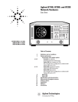
The connections for a typical system are shown above. Other systems
are similar. Follow these suggestions:
Computer system: connect keyboard, mouse, etc with instructions
provided.
Printer (or plotter): connect device to Centronics (parallel)
connector, RS-232 (serial) connector, or HP-IB connector of
computer.
Network analyzer: connect to HP-IB connector of computer.
Cables: connect to ports 1 and 2 of the network analyzer (or test
set, if they are separate instruments).
If your system uses a printer (or plotter, the term is used generically)
and you know how to connect it to the computer, do so now.
Otherwise connect it later, when directed.
Starting the HP
85071 Software
2-6 Getting Started
1. Start up Windows; at the DOS prompt, type:
WIN
1: MS-DOS
Figure 2-2. Windows Program Manager System
2. Double-click on the HP 85071 icon to start the program. The HP
85071 copyright screen appears with the copyright statement.
3. Click in the OK box. The main menu screen (below) replaces the
copyright screen.
Windows Compatible
Software Operation
The HP 85071 materials measurement software is ready for operation
when the copyright statement is replaced with the main menu screen.
Figure 2-3. HP 85071 Main Menu Screen
Getting Started 2-7
1: MS-DOS
Microsoft Windows
Basics
Using the HP 85071 materials measurement software is very similar
to using other Microsoft Windows application programs. Windows
techniques for running application programs include using a mouse,
choosing commands from menus, working with dialog boxes, and
selecting les. Documentation provided with Windows gives a
complete description of the techniques for using Windows. In
this section a very brief overview of basic Windows techniques is
presented.
What Is a Window?
A window is an area on the screen that displays a running (open)
application program. More than one application can run and be
displayed at the same time. Additionally, open windows can be stored
as icons at the bottom part of the screen. This way, an application can
be kept open without showing it as a window in the work area. Each
window is divided into several areas, as shown below.
Figure 2-4.
Graphic Showing a Window, Work Area, and Application Icon
How to Use a Mouse
A mouse is a hand-held pointing device. As the mouse is moved across
the desk, a pointer moves on the screen. Mice have one, two, or three
buttons. All HP 85071 software actions require only one button,
the main mouse button. This is the left-most button on the mouse.
However, on multi-bottoned mice, you can use the right-most button
to trigger a measurement.
2-8 Getting Started
1: MS-DOS
Figure 2-5. Mouse and Location of Main Mouse Button
These terms describe operations with the mouse:
Point to move the tip of the mouse pointer on top of something on
the screen.
Click to quickly press and release the mouse button.
Double-click to quickly press and release the mouse button twice in
succession.
Drag to hold down the mouse button, move the mouse until the
pointer is at the desired location, then release the main button.
Release to quit holding down the mouse button.
Select to point on a menu.
How to Use Drop-Down Menus
Note
Drop-down menus are lists of commands that drop down from the
top of the screen when selected. The names of the software menus
appear on the menu bar at the top of the window displaying the HP
85071 application program.
To select a menu, either
Point to the name of the menu and click the mouse button, or
Press 4Alt5 (the alternate key) and the underlined letter in the name
of the menu. For example, press Alt and \s" for the Setup menu.
To choose a command, do one of the following:
Point to the name of the command on the menu and click the
mouse button
Use an accelerator key on the keyboard: press 4Ctrl5 (the control
key) simultaneously with the accelerator key. Accelerator keys are
identied with a ^ symbol on menus to the right of some of the
commands.
Point to the desired menu with the mouse, drag the mouse
downward to point to the desired command, and then releasing the
mouse button.
Commands that appear in gray do not currently apply and can not be
choosen.
Getting Started 2-9
1: MS-DOS
Figure 2-6. Drop-Down Menu and Highlighted, Selected Command
How to Use Dialog Boxes
A dialog box is a request from the program for information required
to carry out a command. Commands that end in \ . . . " (an ellipsis)
indicate that a dialog box is presented when the command is selected.
Dialog boxes must be lled in before proceeding with program
operation. Some dialog boxes require that you type in text, others
allow you to select options within the dialog box.
To exit a dialog box, select one:
OK keeps all of the changes made in the dialog box
Cancel leaves the dialog box without changing anything
NNNNNNNN
NNNNNNNNNNNNNNNNNNNN
How to Use Dialog Boxes with File Names
Any time a test setup or data le is to be saved or recalled from
disk, the program displays a dialog box. Save and recall dialog boxes
contain two other types of boxes.
List boxes display le names and directories on the chosen disk
(drive).
To change the disk drive, double-click on the drive name (for
example, [-A-]).
To scan the directory, click the arrows on the scroll bars.
To display the les in a directory, double-click on the parent
directory marker (the directory is one level higher in the system's
disk directory organization).
To save or recall a le, double-click on the desired le name.
Note: any of these operations can also be performed by clicking
once in the list box then pointing the mouse to OK and clicking the
mouse button.
NNNNNNNN
2-10 Getting Started
1: MS-DOS
Figure 2-7. Example of Dialog Box
Text boxes provide a space to type directories or le names from the
keyboard.
To see all of the les in a new directory, type the directory name in
the text box. Then click OK .
A le name can be typed into the text box. It can begin with a
drive letter followed, if needed, by a directory name. The le
name itself is usually followed by a three-character le extension.
A period separates the le name and extension. For example,
C:WINDOWSnHP85071nTEST1.TST is a valid le name.
NNNNNNNN
HP 85071 Windows
Software
Fundamentals
The HP 85071 materials measurement software program is a Windows
application program. The techniques for using the HP 85071
software are the same as the techniques used for running other
Windows application programs. The HP 85071 display window and its
components are shown below.
Figure 2-8. Principal Components of the Software Screen
Annotation is the text on the instrument display which describes the
frequency range of the measurement, the permittivity of the MUT, the
format of the display, the scaling of the display, and any display titles.
Grid is composed of the x-axis and y-axis lines on which the data is
plotted.
Instrument display is always present in the window. Most of the
time the instrument display presents measurement data as a graph.
However the data can also be presented as a tabular listing.
Getting Started 2-11
1: MS-DOS
Data trace is a graph of measurement data in the chosen format. It
may be the current trace or one recalled from memory.
How to Exit the Program
To exit the program, point at the small box in the upper left-hand
corner of the display and click the main mouse button.
Conclusion
Tips for Using
Printers and
Plotters under
Microsoft Windows
Software
Setting Up Windows
Control Panel Settings
2-12 Getting Started
Now that you have installed the software and hardware, loaded the
program, and learned the basic operator interface techniques, you
may be ready to make a measurement. If you still need to install a
printer or plotter, continue with \Tips for Using Printers and Plotters
under Microsoft Windows." Otherwise, continue with chapter 3,
\Measurement Tutorial."
The following information applies generally to any printer (or plotter,
the term is used generically) and any MS-DOS personal computers
running Microsoft Windows. Therefore, it does not give exact
instructions, but rather lists general issues that must be addressed to
print successfully.
At best hooking up a printer to a computer is as simple as connecting
the two with a cable. However, computers and printers are each
designed for maximum exibility, so that each can be congured
for a particular system or purpose. Unfortunately, this means that
both must be congured correctly to communicate with each other.
Additionally, in the context of the HP 85071 software, the software,
Windows, MS-DOS, logical and hardware ports, a cable, and the
printer itself must all interact properly to achieve the desired results.
Once you have set up your system, you will use only the interface of
the HP 85071 software to measure materials and store or print the
results. But now you must relate to other, normally invisible, parts of
the system to set it up.
At this time, Windows should have been installed on your computer
by running a program named SETUP. If you have not already installed
Windows, refer to section 1 of chapter 2 to do so. For now, skip the
part of the SETUP program that installs printers by selecting continue.
Through the Windows control panel, you can modify a number of
printer parameters. Run the control panel application. It will let you
install a driver for your printer. Drivers are programs that translate
pictorial information (from an application running under Windows)
into commands a printer can understand. Each dierent kind of
printer has a separate driver designed for it.
Before actually running the control panel application, consult your
printer manual to determine the following:
Name and model number of printer (exactly)
Connection type (serial or parallel)
1: MS-DOS
Handshake (usually hardware)
For serial printers:
Baud rate (how fast it will accept information)
Word length (typically between 4 and 8)
Parity (odd, even, or none)
Stop bits (usually between 1 and 2)
Add New Printer
To install a driver, access the control panel and select the printer icon.
Refer to Windows documentation under \Control Panel" for details.
Documentation in the form of ASCII text les is often included on the
disk containing the drivers. These are READMEx.TXT les.
To list these les, at the DOS prompt type (for example):
dir a:*.txt
To read a le, at the DOS prompt type (for example, on the HP PCL
driver for HP LaserJets):
a:readmehp.txt|more
The purpose of all this is to install exactly the right driver for your
particular printer. Microsoft supplies many driver programs on oppy
disks with the Windows package. You must choose the driver for your
printer and install it (from oppy disk to hard disk) before you can
print. You can install more than one driver, and can have more than
one printer connected to the system at one time; however, only one
printer can be used at a time.
Drivers are updated from time to time, so it is possible that a newer
and better driver is available (to use in place of the one supplied by
Microsoft). Drivers may also be available for printers not supported
by Microsoft.
Contact Microsoft at:
Microsoft Product Support Services 1-206-454-2030
For HP printers and plotters, contact HP at:
HP Customer Support Center 1-208-323-2551 or
Boise Printer Division
Printer/Plotter SUPPORT
Building 21 Mailstop 516
11311 Chinden Blvd.
Boise, ID 83714 USA
Connections
After installing the drivers, Windows must be told which computer
interface to associate (or connect) with each driver. Access the control
panel to do so.
Here, you choose connections such as:
PCL / HP LaserJet on LPT1:
HP Plotter on COM1:
HP QuietJet on None
LPT1 and COM1 refer to the type of hardware interface (or port)
through which computers and printers communicate. You must
determine which type of interface your printer uses and enter that
information. The two main types of interfaces also have associated
logical ports. (A logical port is a specic address and interrupt level
Getting Started 2-13
1: MS-DOS
which the computer associates with a physical port and through
which it communicates.)
Table 2-1.
Interface Common Name
Logical Ports
Serial
Parallel
RS-232
Centronics
COM1, COM2, COM3, COM4
LPT1, LPT2, LPT3
Logical ports are assigned to physical ports by setting small switches
or jumpers on the interface card. These cards are loaded into a \slot"
on the rear panel of the computer. Refer to the computer or interface
documentation to determine what you have and select the logical port
in the control panel accordingly.
A third type of hardware interface exists, called \HP-IB", IEEE-488,
or GP-IB. The computer must also have this interface to control the
network analyzer.
Communications Port
2-14 Getting Started
Control panel settings in Windows can change the serial (RS-232)
communications protocol by overriding denitions in the
AUTOEXEC.BAT le. AUTOEXEC.BAT is an automatically executed
(on power up) batch le located on the root directory. It usually
contains commands to congure the communications ports.
Windows ignores AUTOEXEC.BAT commands when controlling
a printer via a serial port. However, if a printer was working
successfully before installing Windows, it may help to examine
AUTOEXEC.BAT (as explained below) and modify the communications
port settings to match it.
Parallel ports are not aected by Windows.
Several parameters dene the communications protocol used by
serial (RS-232) ports. The protocol must match that of the printer.
Some printers are capable of changing their serial protocol, via small
switches or other controls. Refer to the printers manual for details.
These are the parameters and most common values for HP printers:
BAUD rate: 9600, 4800, 2400, 1200, 19200, 300
Parity: None, Even, Odd
Number of data bits (word length): 8, 7, 6
Number of stop bits: 1, 1.5, 2
Handshake type:
Hardware (DTR, Printer Busy)
None (XON/XOFF)
To change the communications protocol used by Windows, access the
control panel and enter the changes.
1: MS-DOS
The AUTOEXEC.BAT
File
Commands that congure a serial port typically look like this: MODE
COM1:9600,N,8,1 If the printer is connected to a parallel port, the
mode command may look like this: MODE LPT1:,,P
Note that the MODE command can also redirect the printer from one
logical port to another. The default printer is usually assumed to
be at LPT1. If the printer is a serial type, the printer data may be
redirected via LPT1 to COM1 with this command: MODE LPT1:=COM1:
If needed, the AUTOEXEC.BAT le can be modied with EDLIN or
other ASCII text editors. Refer to DOS documentation for details on
the \MODE" command.
After editing AUTOEXEC.BAT, restart the computer to read and
execute the edited le. Press 4CTRL5 + 4ALT5 + 4DEL5 to do so.
Other les can have an eect on printer performance, though not as
often as AUTOEXEC.BAT. Those les are described below in \Other
Files Worth Knowing About."
Cables
A cable is needed to connect printer to computer. There are many
cables to choose from. Do not assume that a cable with connectors
that merely \mate" correctly at each end will work correctly; this is
rarely the case.
The choice of cable is based on:
Printer model
Type of interface (serial RS-232, or parallel Centronics)
Connector type at each end (e.g. 9-pin, 25-pin, or 36-pin)
Sex at each end (male or female)
For HP printers, the Computer Users Catalog provides an excellent
look-up table to help choose the correct cable. To request a catalog, or
to order cables and adapters with a credit card, call:
HP DIRECT ORDERING at 1-800-538-8787 (toll-free from US)
Outside the US, similar services are usually available locally. Refer
to your local phone directory under \HP", or call these numbers
(international toll call to the US):
U.S.A. 408-553-7800 (for information on local services)
U.S.A. 415-857-5027 (to place an order from a non-US country)
Printer Settings
Most printers can be congured or set by the user with small switches,
jumpers, or buttons. Settings fall into two categories: serial and mode.
Serial settings select the protocol used by the serial port. The
protocol includes BAUD rate, parity, word length, and handshake.
See printer's manual for recommendations, and see \Communications
Port" to make sure the computer's serial port protocol matches the
printer.
Mode settings control how the printer responds to certain commands
(after being received correctly via the communications port). Settings
may aect: response to CR, response to LF, page size, font selection,
font size, etc.
Getting Started 2-15
1: MS-DOS
Some HP printers have a mode switch that selects between
\Alternate" and \HP" mode. Use the \HP" setting, unless using a
non-HP driver.
\Dene plot " in
the HP 85071
Software
...
Other Files Worth
Knowing About
Conclusion
2-16 Getting Started
Once you are running the HP 85071 software, select Output then
Define Plot... to specify the printer driver you want to record
measurement results. This selection points to a driver in Microsoft
Windows, described above.
If that driver supports more than one printer, the printer must already
have been chosen in the control panel. The control panel also selects
the hardware port to which the output will be sent, and the protocol
(used by a serial port). The port and protocol selected must match the
actual port and protocol used (often user settable) on the printer.
NNNNNNNNNNNNNNNNNNNN
NNNNNNNNNNNNNNNNNNNNNNNNNNNNNNNNNNNNNNNNNNNN
CONFIG.SYS is another le (on the root directory) containing
commands which are executed when the computer is started. It
may contain references to device drivers such as keyboard, mouse,
display, hard disk, etc. CONFIG.SYS may act in the same way as
AUTOEXEC.BAT, but it is more common to edit AUTOEXEC.BAT as
explained above.
WIN.INI is a le that Windows reads when starting up. It is usually
in the Windows directory. It stores default settings of the HP 85071
program such as frequency, number of points, type of sweep, etc.
To edit these settings:
1. Use a text editor.
2. Page down to [HP 85071B].
3. Edit as desired.
4. Save and exit.
This information is only a summary. If you are unable to successfully
print or plot within the HP 85071 software program, do not hesitate
to review the documentation of Windows, the printer, the cable, and
the interface.
2: HP BASIC
SECTION 2: HP
BASIC Version of
the Software
System
Requirements
To run the HP BASIC version of the HP 85071 software program,
you must have a HP BASIC-compatible computer as dened below.
Additionally, you should be familiar with basic BASIC operations.
The system requires the computers, software, interfaces, printers and
plotters, and network analyzers described below.
Computer
The HP 85071 software supports the HP Vectra PC (with BASIC
language processor card) and all HP 9000 series 300 computers except
these:
HP 9817
HP 9826
HP 9837
HP 9920
The minimum requirements for the computer are these:
2.0 MBytes (minimum) of RAM (Random Access Memory)
High-density, double-sided 3.5 inch exible disk drive
HP 82300C (required for HP Vectra PC)
HP 82304A high performance measurement co-processor (required
for HP Vectra PC)
BASIC and Binaries
The computer must have BASIC operating system version 5.0 (or
higher) and these binaries:
COMPLEX
CS80
ERR
GRAPH (GRAPHX if color CRT)
HPIB
IO
MAT
MS
Other binaries may be present in the BASIC operating system but,
when additional binaries are present, the computer may require more
than 2.0 MBytes RAM.
The HFS (hierarchical le system) binary can also be used to specify
volumes and directories for saving program information.
The HP 85071 software will also run under the HP-UX system with
HP-RMB-UX BASIC language support.
Getting Started 2-17
2: HP BASIC
IEEE-488 (HP-IB)
Interface
The computer must have an HP-IB interface to control the network.
Printers and Plotters
An HP-IB printer can be used to produce tabular listings of
measurement results or printer facsimiles of graphed data. A number
of HP-IB printers may operate properly with the software but have
not been tested. The following printer has been tested to insure
compatibility with the program and is therefore recommended for use
with the software:
HP 2225A, ThinkJet printer with HP-IB interface option
HP-IB plotters can also be used to produce hardcopy graphs of the
data. A number of HP-IB plotters may operate properly with the
software but have not been tested. The following plotters have been
tested to insure compatibility with the program and are therefore
recommended for use with the software:
HP 7440A ColorPro eight-pen plotter with HP-IB interface option
HP 7470A two-pen graphics plotter with HP-IB interface option
HP 7475A two-pen graphics plotter with HP-IB interface option
HP 7550A graphics plotter
Network Analyzer and
Test Set
The HP 85071 software is designed to work with the network analyzer
congurations described below. The default HP-IB address is 16.
HP 8752A: this network analyzer contains a reection/transmission
test set as part of the analyzer. No other instrumentation is needed
to make measurements. The network analyzer has these limitations:
\Re/Tran u & e N-R" model: supported in the accurate sample
position denition mode
\Re/Tran e Prec'n" model: not supported
\Re/Tran e Fast" model: supported in the accurate sample
position denition mode
HP 8753A, B, or C: these network analyzers need a companion test
set for operation with the software. The following test sets are
supported:
HP 85044A reection/transmission test set (subject to the same
limitations as the HP 8752A)
HP 85046A S-parameter test set
HP 85047A S-parameter test set
HP 8719A or C; HP 8720A, B or C; HP 8722A or C: these network
analyzers contain S-parameter test sets as part of the analyzer. No
other instrumentation is needed to make measurements.
HP 8510B or C: this network analyzer requires a companion test
set and a synthesized source for operation with the software.
Frequency range is determined by the test set and source. All test
sets supported by the HP 8510B are supported by the software.
The HP 8340, HP 8341, or HP 8360 family sources are supported
by the software. HP 8510B or C rmware revision 5.0 or higher is
required.
2-18 Getting Started
2: HP BASIC
Note
Installation
The HP 8510A is not supported by the software but can be upgraded
to an HP 8510C with the HP 85103C upgrade kit.
HP BASIC Installation
The Hewlett-Packard BASIC operating system (version 5.0 or higher) is
required for the HP 85071 software. Additionally, the BASIC system
must include the previously listed binaries for operation with the HP
85071 software. Refer to the computer's manual set for additional
information on installing or conguring the BASIC operating system.
HP 85071 Software Installation
The HP 85071 software program resides in a single le on the HP
85071 program disk. The name of the le is HP85071B.
The HP 85071 program should be copied to a working disk so that the
original disk can be stored as a back-up. Thus, if the (new) working
copy is damaged or lost, the back-up is still available.
Use the COPY command in HP BASIC to copy the program to another
disk drive. The syntax of the COPY command is:
COPY "FILENAME:MSUS" to "FILENAME:MSUS"
where MSUS is short for mass storage unit specier. MSUSs are
typically of the form \,700,1" where \,700" is the drive address and
\1" is the drive number. For example, to copy the program from drive
address 700, drive 0 to drive address 700, drive 1, type:
COPY "HP85071B:,700,0" TO "HP85071B:,700,1"
Refer to the BASIC operating system manuals for more information of
mass storage speciers and the COPY command.
Hardware Installation
Connect the computer, network analyzer, cables, and peripherals, as
shown below. For HP 8753 systems, refer to the network analyzer
documentation to connect the test set. For HP 8510 systems, refer
to the network analyzer documentation to connect the test set and
source.
Dierent systems require various cables and adapters. These items
are listed in HP's RF, Microwave, & Millimeter Wave Measurement
Accessories Catalog and the Test and Measurement Catalog.
Getting Started 2-19
2: HP BASIC
Figure 2-9. Typical HP BASIC System Connection Diagram
The connections for a typical system are shown above. Other systems
are similar. Follow these suggestions:
Computer system: connect keyboard, mouse, etc with instructions
provided.
Printer (or plotter): connect device to HP-IB connector of computer.
Network analyzer: connect to HP-IB connector of computer.
Cables: connect to ports 1 and 2 of the network analyzer (or test
set, if they are separate instruments). Torque the connectors to ve
inch-pounds.
Starting the HP 85071
Software
2-20 Getting Started
To start the HP 85071 software program, follow these steps:
1. To load the software from the working copy into memory, type
LOAD "HP85071B" and press 4ENTER5 or 4RETURN5
When the disk access annunciator in the bottom right of the
computer CRT goes out, the program is loaded. If the system does
not respond as expected, change the mass storage unit with the
MSUS command.
2. To run the program, type RUN or press 4RUN5.
The HP 85071 program's copyright screen will now appear
displaying the copyright statement.
3. To erase the statement and view the main menu screen, press
4ENTER5 or 4RETURN5.
The HP 85071 software is ready for operation when the main menu
screen (shown below) replaces the copyright statement.
2: HP BASIC
Figure 2-10. HP BASIC Main Menu Screen
HP BASIC Software
Operation
As explained below, the HP 85071 software uses softkeys and menus
to interact with the operator.
What are Softkeys?
Softkeys are keys which are relabeled to perform dierent functions
as the program runs. The labels for the softkeys are located on the
bottom of the computer display. The softkey labels correspond to the
function keys (F1 through F8) on the computer keyboard.
The softkeys are labeled with the names of the menus in the program.
Pressing a menu softkey brings up that menu of choices for working
with the program. Any time the softkeys are labeled, they are active
and can be used to select a menu. Sometimes during the program the
softkeys are relabeled. When input from the keyboard is required,
the softkeys are labeled with terminators for the entry. For example,
if start frequency is being entered, the softkeys are re-labeled GHz,
MHz, KHz, and Hz.
How to Use Menus
Menus are lists of commands or other menus or both. When a menu is
selected in the HP 85071, menu choices, or commands are presented
in the upper right portion of the computer's display. The various
menus in the software are found on the softkeys at the bottom of the
computer display.
To select a menu, press the function key on the keyboard that
corresponds to the menu softkey on the computer display. The menu
choices will appear on the upper right portion of the display with a
cursor arrow pointing to one of the commands in the menu.
To choose a command, use the UP/DOWN cursor (arrow) keys to point
the cursor arrow to the desired command. Then press 4RETURN5 or
4ENTER5 to select that command. Some commands take immediate
action, for example the autoscale command. Other commands require
additional keyboard input. Those commands present a menu of
selections.
Getting Started 2-21
2: HP BASIC
How to Make Menu Selections
Use the UP/DOWN arrow keys to point to the entry parameter or
choice. Then press 4RETURN5 or 4ENTER5.
If the choice requires keyboard entry (frequency entry, Y-axis scale
entry, etc.), the software displays a prompt for input. The softkeys
are labeled with terminator units for the input (GHz, MHz for
frequency entry; etc.) Type the desired response to the prompt on the
keyboard and use the appropriate softkey to terminate the entry.
To nish the selection, press one:
OK to keep all of the new entries
Cancel to leave the old entries unchanged
NNNNNNNN
NNNNNNNNNNNNNNNNNNNN
Figure 2-11. HP BASIC Sample Menu Selections
HP 85071 HP BASIC
Software
Fundamentals
The HP 85071 display window and its components are shown below.
Figure 2-12.
Main Menu Screen with Pull-Outs Describing Principal Functions
of Components
The instrument display is always present. Most of the time the
instrument display presents measurement data as a graph. But it can
also present the data as a tabular listing.
2-22 Getting Started
2: HP BASIC
These terms refer to parts of the instrument display: Grid is
composed of the x-axis and y-axis graticules on which the data is
plotted.
Traces are graphs of measurement data. They are the measured
values of permittivity plotted on the grid. When the software rst
starts up, no measurement traces are presented.
Annotation is the text on the instrument display which describes the
frequency range of the measurement, the format of the display, the
scaling of the display, and any display titles.
Conclusion
Now that you have installed the software and hardware, loaded the
program, and learned the basic operator interface techniques, you
are ready to make a measurement. Please continue with chapter 3,
\Measurement Tutorial."
Getting Started 2-23
Measurement Tutorial
Introduction
Section 1: General
Overview
Sample Shapes
3
The ve sections of this chapter provide a tutorial introduction to the
HP 85071 materials measurement software.
1: General Overview summarizes the measurement and data
reduction process.
2: Calibration Considerations discusses calibrating various
network analyzer for use with the software.
3: Sample and Sample Holder Considerations compares the
dierent types of sample holders and the preparation of materials
samples.
4: Measurement Models reviews each of the data reduction
models available for use with the software.
5: Waveguide Calibration and Measurement Example is a
step-by-step example procedure of a waveguide calibration and
measurement.
The software is designed to calculate materials properties, complex and , from the S-parameter measurements of a sample in waveguide
or coaxial transmission line or free space.
Each type of \transmission line" requires a dierent shape sample and
sample holder.
waveguide: sample is brick-shaped; sample holder is a section of
waveguide transmission line
Coax: sample is donut-shaped; sample holder has a precision
connector, such as 7mm, at each port and a precision center
conductor
Free space: sample is at; sample holder varies.
Measurement Tutorial 3-1
1: General Overview
Figure 3-1.
Samples in Coaxial and Waveguide Transmission Lines and Free
Space
Calibrating the
System
The software requires that you manually calibrate the network
analyzer measurement system before making a measurement.
Calibration removes measurement uncertainties from the system. If
possible, calibrate with the sample holder connected to port 2 (for
reasons, see sections 2 and 3, following).
After calibration, minimize changes to the measurement system
such as cable movement and temperature variations. More detailed
information on the calibration process can be found in the network
analyzer's documentation. A calibration example concludes this
chapter.
Measuring the MUT's
S-Parameters
After calibration, the network analyzer measures the S-parameters of
the sample holder and sample material. The measurements may be
reection measurements, transmission measurements, or both. The
raw measurements of the sample holder and sample material are then
vector error corrected using the system error model obtained during
the calibration process. The corrected S-parameters are transferred to
the computer.
Converting the
S-Parameters to and
The computer mathematically rotates the S-parameters through the
appropriate lengths of transmission line. These lengths are input to
the software during setup. At this point the S-parameters represent
the S11 and S22 input reection coecients at the sample interfaces,
the S21 and S12 transmission through the sample, or both. The
software uses the S-parameters at the sample interface to calculate
the complex permittivity and permeability.
Various models are available with the HP 85071 for converting the
S-parameters of the material sample to permittivity and permeability.
Descriptions of each model are presented later in this chapter
3-2 Measurement Tutorial
1: General Overview
and in chapter 8. Some of the models use iterative calculation
routines. As with all iterative routines, it is important to provide an
estimate of the solution to start the calculation. The software has
built in algorithms for obtaining estimates to start the calculations.
Unpredictable results can be overriden with the \verify estimate"
command in the setup menu. This presents the estimate that the
software is making for the materials parameters at the rst frequency.
If incorrect, the estimate may be overridden at this point.
Measurement Tutorial 3-3
2: Calibration Considerations
Section 2:
Calibration
Considerations
Calibration Notes
Take care to store, maintain, and clean the calibration standards
properly. Refer to Hewlett-Packard Application Note 326: Coaxial
Systems Principles of Microwave Connector Care for reference
information.
Calibrate the system with the sample holder connected to the cable
(or waveguide adapter) at port 2 for best results. If this is not
possible, calibrate at the connection interface to the sample holder.
For a coaxial holder, this is at the end of the test cables that attatch to
the sample holder. For the waveguide holder, this is at the waveguide
ends of the coax-to-waveguide adapters.
Set frequency before calibration
Calibrate the system manually, from the front panel of the network
analyzer
Calibrate with the sample holder in place if possible (see following
section for details)
Minimize cable movement after calibration
Use sample holder same length as sample to avoid holder losses
Table 3-1.
Required Calibrations and S-parameter
Measurements for Calculation Models
Model Name
Calibration Measured S-Parameters
Re/Tran u & e N-R Full 2-Port
One Path 2-Port
Re/Tran e Prec'n Full 2-Port
Re/Tran e Fast
Full 2-Port
One Path 2-Port
Re e Short-Back S 1-Port
Re e Arbit-Back S 1-Port
Re u & e Sing/Dbl S 1-Port
11
11
11
HP 8510
Considerations
3-4 Measurement Tutorial
S
S
S
S
S
S
S
S
11
11
11
11
11
,S ,S ,S
,S
,S ,S ,S
,S ,S ,S
,S
21
12
22
21
12
22
21
12
22
21
21
11
11
11
Calibrations and measurements should be made with the signal source
in a synthesized mode of operation at each measurement frequency.
With the HP 8510 this dictates the use of the stepped CW (STEP in
the stimulus menu) sweep mode. When the HP 8510 is used in the
stepped CW mode, 128 averages can be used without aecting the
measurement speed appreciably.
Measurements with the HP 8350 sweeper are not supported with the
HP 85071 software.
2: Calibration Considerations
HP 8719, HP 8720,
HP 8722, HP 8753
Considerations
Reection/Transmission
Test Set
Considerations
Calibrations and measurements should be made with the signal
source in a frequency step mode of operation at each measurement
frequency. There is a minimum sweep time which allows the analyzer
to operate in the step mode. This minimum sweep time is a function
of sweep range, IF bandwidth, and the number of measurement
frequencies.
If an \arrow" follows along the trace of the network analyzer CRT as
a sweep is taken, the analyzer is in step mode. If not, either reduce
the IF bandwidth (the preferred tactic) or increase the sweep time
enough for the analyzer to operate in step mode.
Reection/transmission test sets are subject to some limitations.
Examples of such tests sets are the HP 85044 (used with the HP 8743)
and the built-in HP 8752 test set. These are the limitations:
\Re/Tran u & e N-R" model: supported in the accurate sample
position denition mode only
\Re/Tran e Prec'n" model: not supported
\Re/Tran e Fast" model: supported in the accurate sample position
denition mode only
Measurement Tutorial 3-5
3: Sample and Sample Holder Considerations
Section 3: Sample
and Sample Holder
Considerations
Sample Holder
Coaxial versus
Waveguide Sample
Holders
Free Space
Dimensions of Holder
and Sample
The software assumes that the sample holder is well matched and
has negligible loss. Only the phase shift of the known lengths of
transmission line is accounted for. Use only a precision, well-matched
sample holder. Connect it to port 2 prior to calibration. Any
reections o the input or output of the sample holder will degrade
the calculated material parameters.
For best measurement results, the sample should ll the cross-section
of the transmission line with no air gaps.
Coaxial sample holders have the inherent advantage of being
broadband. They are however, typically harder to construct for
the ease of sample loading. Coaxial samples also require more
preparation. Waveguide sample holders are limited to use in the
waveguide frequency band. However, they can be easy to fabricate
and require less sample preparation.
Free space samples should be at; material preparation may be
unnecessary. This type of material measurement is broadband. Rather
than the material being contained within a transmission line, antennas
radiate energy through the sample. Air gaps are not a problem with
this technique.
The sample holder length, distance to sample, and sample thickness
are entered in the sample holder . . . menu. The thickness and
distance information needs to be characterized as accurately as
possible.
Sample Holder Length
This is the length of transmission line added to the measurement
path after calibration. For both coaxial and waveguide lines, it is
the distance between the outer conductor mating surfaces. In other
words, it is the actual length added to the transmission path when
the sample holder is tightened in place. It should be calibrated out or
precisely measured.
To calibrate out the sample holder length: connect the sample
holder to port 2 during calibration as shown below. Then calibrate the
system using the sample holder as one of the calibration reference
planes. Note that since additional transmission line is not added after
calibration, the holder length is 0 (zero).
3-6 Measurement Tutorial
3: Sample and Sample Holder Considerations
Figure 3-2. Samples in Waveguide, Coaxial and Free Space
To calibrate without the sample holder in place, measure the
holder mechanically as precisely as possible. Enter this length in the
sample holder menu. As shown below, the calibration reference
planes are the ends of the waveguide adapters (or coax cable ends).
Figure 3-3. Sample Holder Reference Planes
To verify the sample holder length after calibration:
Attach the sample holder to the calibration reference planes.
Measure the sample holder \empty".
If the dielectric constant is calculated as about 1.0006 (air), the
length is correctly entered.
If the value is not about 1.0006, vary the entered length and use
the recalculate feature to close in on the correct number.
If the value does not approach 1.0006, recalibrate the system (see
section 5 for an example).
Distance to Sample
This dimension is the distance from the port 1 calibration reference
plane to the sample. It should be precisely measured when required
by the model. Any inaccuracy in this distance causes the \rotated"
S-parameters to be in error. This is the most dicult distance
measurement to make in that the sample must be loaded in the
Measurement Tutorial 3-7
3: Sample and Sample Holder Considerations
sample holder to measure the distance. Some of the models do not
depend on precisely knowing the position of the sample in the sample
holder.
In many cases, the simplest way to determine the distance to sample,
is to place it ush with the port 1 calibration reference plane. Then
the distance is simply 0 (zero), and 0 should be entered in the sample
holder . . . menu.
Sample Thickness
This should be measured by the most accurate mechanical means
available (micrometer, vernier caliper, etc.). Uncertainty in the
sample thickness will cause inaccuracies in the calculated materials
parameters. The inaccuracy due to thickness errors increases with
frequency and increases with the magnitude of and .
Table 3-2.
Calculation Models and Optimum Sample Thickness
Calculation Model
Optimum
Sample Thickness
Re/Tran u & e N-R
Re/Tran e Prec'n
Re/Tran e Fast
Re e Short-Back
Re e Arbit-Back
Re u & e Sing/Dbl Thk
/4
n /2
n /2
/2
/2
/4 & /2
g
g
g
g
g
g
g
Note:
g
=q
r
0
3 r 0
0 12
0
c
where, for TE mode in rectangular waveguide:
c = speed of light (about 3x10 m/sec)
= c/frequency
= relative permittivity
= relative permeability
a = width of broad wall of waveguide
= 2a
10
8
0
r
r
c
Other Factors
These include sample composition and t. It is important that the
sample be uniform and completely ll the guide in the transmission
line sample holder. Any air gaps between the sample and the center
or outer conductor will cause measurement errors. The sample should
t tightly in the holder and be free of nicks.
3-8 Measurement Tutorial
3: Sample and Sample Holder Considerations
Air Gap Correction
Gaps between the sample and its transmission line holder may
dominate the uncertainties of the measurement, especially for high
permittivity materials. The air gap correction function of the software
moderates this eect. This function is part of the sample holder
command in the setup menu. For details, see \Setup Menu, Air Gap
Calculations" in chapter 8, \Software Reference."
Figure 3-4. Air Gap Correction Figure
Air gap correction applies to coax and waveguide measurements, not
free space. It is based on work presented in NIST technical note 1355
(see chapter 7, \Ordering Supplies," for listing).
Measurement Tutorial 3-9
4: Measurement Models
Section 4:
Measurement
Models
Six dierent measurement/calculation models are available in the
software. Each model has dierent advantages and limitations. The
use of each model is determined by several factors:
Optimum sample length (see previous table)
Measured S-parameters (see table below)
Desired measurement parameters
Speed versus accuracy trade-os
Model Name
Table 3-3. Measurement Models
Measured
Comments
S-Parameters
Re/Tran u & e N-R all or S , S
11
Re/Tran e Prec'n
Re/Tran e Fast
Re e Short-Back
Re e Arbit-Back
Re u & e 2 Pos/Thk
21
all
S
S
S
11
11
11
r
r
r
all or S , S
11
e * & u *, fast but has
discontinuities, best for magnetic,
short, or lossy MUTs
e *, accurate, no discontinuities,
best for long, low-loss MUTs
e *, similar to Precision but faster
and better for lossy MUTs, best for
long, low-loss MUTs
e *, best for liquids or powders
e *, best for thin lms
e * & u *, reection only, requires 2
measurements, slow, best for liquid,
powder, magnetic, materials
21
r
r
r
r
r
For details, do one:
Select the measurement model of interest in the setup menu
Refer to chapter 8, \Software Reference"
3-10 Measurement Tutorial
5: Waveguide Calibration
Section 5:
Waveguide
Calibration and
Measurement
Example
Note
How to Begin a
Waveguide
Calibration
This is an example of an X-band waveguide calibration and
measurement with a MS-DOS driven HP 8720 vector network analyzer
system. If you are not familiar with network analyzers, waveguide,
or the calibration process, you should read and perform this example
sequence before measuring your MUT.
If you are using another network analyzer or a coaxial-based
measurement, you may have to adapt this sequence to your setup.
The basic sequence for all of the analyzers is quite similar, but if you
need additional, specic information, refer to the documentation of
the network analyzer.
Before you can make a measurement, you must manually calibrate
the network analyzer. In the case of waveguide, you must rst load
the waveguide cal(ibration) kit information into the network analyzer
before the computer takes control of the system. Then you can
proceed with the calibration (including setting the frequency range).
If you have not yet congured the hardware or loaded the software
for your system, refer to chapter 2, \Getting Started."
Turn o the system computer. Connect a disk drive to the network
analyzer with an HP-IB cable. Turn on the drive and analyzer. Insert
the calibration kit disk in the drive. For the HP 8720, press 4LOCAL5
SYSTEM CONTROLLER 4RECALL5 LOAD FROM DISK LOAD WR90 to load
the waveguide cal kit data into the analyzer.
Note that when the information is correctly loaded, the frequency
range of the analyzer changes to match that of the cal kit (in this
example, 8.2 to 12.4 GHz). If the analyzer does not seem to load the
cal kit data, check that each instrument is set to its default HP-IB
address: drive = 0; analyzer = 16.
If your cal kit does not include a cal data disk, refer to the cal kit
and network analyzer manuals to see how to enter the cal kit data
manually.
Press 4LOCAL5 TALKER-LISTENER to end network analyzer control of
the HP-IB bus.
NNNNNNNNNNNNNNNNNNNNNNNNNNNNNNNNNNNNNNNNNNNNNNNNNNNNN
NNNNNNNNNNNNNNNNNNNNNNNNNNNNNNNNNNNNNNNNNNNN NNNNNNNNNNNNNNNNNNNNNNNNNNNNN
NNNNNNNNNNNNNNNNNNNNNNNNNNNNNNNNNNNNNNNNNNNNNNN
Start the HP 85071
Software Program
Turn on the computer (it too should be connected to the analyzer
with an HP-IB cable). Start the program as explained in the previous
chapter. The copyright screen should appear. Continue.
Notice that as the software program begins, it resets the analyzer to
the cal kit frequency range in polar chart format.
Measurement Tutorial 3-11
5: Waveguide Calibration
Set Up the
Measurement First
In general, the rst step in setting up the system for calibration
and measurement is to select the frequency range (a start and stop
frequency, and either the number of frequency points or a step
frequency).
The measurement frequency range:
Must match the calibration frequency range
Can be as wide as the bandwidth of the cal kit
Can be just part of the bandwidth of the cal kit
1. Click on 4Setup5
2. Select Set frequency... to display the dialog box below
NNNNNNNNNNNNNNNNNNNNNNNNNNNNNNNNNNNNNNNNNNNNNNNNNN
Figure 3-5. Set Frequency . . . Dialog Box (MS-DOS Version)
Change Start Frequency to 8.2 (GHz)
If loading the cal kit data made this setting, skip to the next
paragraph.
1. Move the pointer to the text box just to the right of Start freq
2. Click at the far left end of the text box, drag across to the far
right end of the text box, and then release the mouse button. This
highlights the entire current entry.
3. Type in 8.2 (You do not have to enter the units, GHz, as that is the
default value.)
Do NOT select OK or press 4RETURN5 or 4ENTER5 yet.
NNNNNNNN
Change Stop Frequency to 12.4 (GHz)
If loading the cal kit data made this setting, skip to the next
paragraph.
1. Move the pointer to the left end of the Stop freq text box.
2. Click, drag, and release as above.
3. Type in 12.4
3-12 Measurement Tutorial
Change Num Pts to 51
5: Waveguide Calibration
Change the number of points to 51, as above.
OK the Changes and Exit the Dialog Box
In this example, we use the default values for units (GHz) and sweep
mode (linear).
To accept the settings made, do one:
Select OK command with the mouse
Press 4ENTER5 or 4RETURN5 on the keyboard
The software displays the hourglass as it updates the network
analyzer.
NNNNNNNN
Dene the Model
This dialog box lets you select the measurement model.
Figure 3-6. Model . . . Dialog Box (MS-DOS Version)
1. Select 4Setup5
2. Select Model... (note that the current measurement model is
\Re/Tran u & e N-R")
3. Select Cancel to leave the dialog box without changing it
NNNNNNNNNNNNNNNNNNNNNNNNNN
NNNNNNNNNNNNNNNNNNNN
Measurement Tutorial 3-13
5: Waveguide Calibration
Dene the Sample
Holder
Note
If you are using a coaxial system, or a dierent waveguide cal kit,
enter the equivalent data. The software lookup table (explained
below) and the \Software Reference" chapter contain tables of
common waveguide cuto frequencies. The cuto frequency for
coaxial systems is 0 GHz.
This example assumes this hardware conguration:
Cable connected to port 1
Waveguide adapter connected to port 1 cable
Cable connected to port 2
Waveguide adapter connected to port 2 cable
Sample holder connected to port 2 waveguide adapter
Calibrate the system with the sample holder in place whenever
possible. This technique removes uncertainties in sample holder
length and to a rst order removes sample holder loss. For details,
refer to \Sample and Sample Holder Considerations" earlier in this
chapter.
To perform this calibration example,
1. Select 4Setup5
2. Select Sample holder... to enter the sample holder description
dialog box.
3. Enter this information for the X-band waveguide cal kit:
Sample holder length: 0(default)
Distance to sample: 0 (default)
Sample thickness: (enter non-zero value)
Units: inch (default)
Sample holder: Waveguide
Click on Lookup table>>
Select \X Band W/G 8.20-12.4 GHz"
Click on OK to leave the lookup table (note that it sets the
cuto frequency)
4. Click on OK to exit the dialog box
NNNNNNNNNNNNNNNNNNNNNNNNNNNNNNNNNNNNNNNNNNNNNNNNNN
NNNNNNNNNNNNNNNNNNNNNNNNNNNNNNNNNNNNNNNNNNNN
NNNNNNNN
NNNNNNNN
3-14 Measurement Tutorial
5: Waveguide Calibration
Figure 3-7.
Sample Holder Description Dialog Box (MS-DOS Version)
Perform the
Calibration
The calibration consists of measuring known standards and using
the results to characterize the three major sources of measurement
error. A full 2-port calibration consists of reection, transmission, and
isolation measurements. Isolation should be omitted in most instances.
The default calibration standards are a pair of short circuits, a \thru,"
and a load.
The shorts are
a ush short and a 1/4 wavelength oset short, or
a 1/8 and 3/8 wavelength oset short
The \thru" consists of simply butting the two waveguide anges
together
Loads may be xed, sliding, or oset.
NOTE: in the following example, softkey and hardkey names may
vary from cal kit to cal kit and from analyzer to analyzer.
To begin the calibration, on the network analyzer,
1. Press 4LOCAL5 CAL CAL KIT USER KIT . The user kit should be
dened as WR-90 (because you previously loaded it from disk).
2. Press 4CAL5 CALIBRATE MENU FULL 2-PORT REFLECT'N to enter
the rst part of the calibration sequence.
NNNNNNNNNNN NNNNNNNNNNNNNNNNNNNNNNN NNNNNNNNNNNNNNNNNNNNNNNNNN
NNNNNNNNNNNNNNNNNNNNNNNNNNNNNNNNNNNNNNNNNNNN NNNNNNNNNNNNNNNNNNNNNNNNNNNNNNNNNNN NNNNNNNNNNNNNNNNNNNNNNNNNNNNN
Stabilize the Cable and Measure the First Standard (Flush
Short)
Cable movement degrades measurement accuracy. Before you
calibrate, immobilize the cables and adapters: lay the cables at on a
work surface or hold them in place.
Measurement Tutorial 3-15
5: Waveguide Calibration
Note
Figure 3-8. Measuring the Flush Short
Measurement degradation can result from changing the position of the
cable between calibration and measurements. Keep such changes and
exures to a minimum.
The reection calibration softkeys should now be visible on the
network analyzer display. The top softkey is labelled \S(11): SHORT."
S11 means it is a reection measurement at port 1.
1. Connect a ush short to the port 1 waveguide adapter.
2. Press S11: SHORT to measure the short.
3. Remove the short when the analyzer beeps or underlines the
softkey label.
NNNNNNNNNNNNNNNNNNNNNNNNNNNNNNNN
Measure the Second Standard (1/4 Wavelength Oset Short)
Figure 3-9. Measuring the 1/4 Wavelength Oset Short
1. Connect a 1/4 wavelength oset short to the port 1 waveguide
adapter.
2. Press 1/4 OFFS (immediately below the \(S11): SHORT" softkey)
to measure the short.
3. At the beep or underline, remove it.
NNNNNNNNNNNNNNNNNNNNNNNNNN
Measure the Third Standard (Fixed Load)
Figure 3-10. Measuring the Fixed Load
1. Connect the xed load to the port 1 waveguide adapter.
2. Press FXD LOAD (immediately below the previous softkey) to
measure the xed load.
3. At the beep and underline, remove it.
NNNNNNNNNNNNNNNNNNNNNNNNNN
3-16 Measurement Tutorial
5: Measurement Example
Measure the Three Standards at Port 2
Use the same three standards and the next three softkeys (in the
S22 group) to calibrate port 2 as above. Whereas the standards were
connected directly to the waveguide adapter at port 1 of the analyzer,
at port 2 connect the standards to the sample holder attached to the
waveguide adapter.
Press REFLECT'N DONE after you have measured all of the standards
once at each port (waveguide ange).
NNNNNNNNNNNNNNNNNNNNNNNNNNNNNNNNNNNNNNNNNNNN
Measure the Transmission Standards
Figure 3-11. Measuring the Thru
1. Connect the two waveguide anges together (with the sample
holder between them).
2. Press TRANSMISSION .
3. Make all four transmission measurements, two forward and two
reverse.
4. Press TRANS. DONE when all four softkeys are underlined.
NNNNNNNNNNNNNNNNNNNNNNNNNNNNNNNNNNNNNN
NNNNNNNNNNNNNNNNNNNNNNNNNNNNNNNNNNN
Conclude the Calibration
Finish the calibration without isolation.
1. Press ISOLATION OMIT ISOLATION ISOLATION DONE and
DONE 2-PORT CAL .
The network analyzer calculates the error-correction numbers and
displays the notation \C2" at the upper left of the display when done.
NNNNNNNNNNNNNNNNNNNNNNNNNNNNN NNNNNNNNNNNNNNNNNNNNNNNNNNNNNNNNNNNNNNNNNNNN NNNNNNNNNNNNNNNNNNNNNNNNNNNNNNNNNNNNNNNNNNNN
NNNNNNNNNNNNNNNNNNNNNNNNNNNNNNNNNNNNNNNNNNNNNNN
Measurement Tutorial 3-17
5: Measurement Example
Measure a Sample
Material
With the sample holder between the two waveguide anges, measure
a MUT, air (easily available, no t problems).
1. Select 4Measure5 in the main menu.
2. To make the measurement, do one:
Select Trigger meas in the measure menu
Click the right mouse button
The software initiates the measurement, calculates the complex
permittivity and permeability, and displays the permittivity results.
The initial results are presented on the default scale of 0 to 20 in the
e0 versus frequency format as shown below.
NNNNNNNNNNNNNNNNNNNNNNNNNNNNNNNNNNNNNN
Figure 3-12. Default Display of Air Measurement
Scale the Display
Each format is displayed in the scale last used for that format.
To change the scale of the software display,
Select 4Scale5 in the main menu screen.
Select the three commands in turn to scale the y-axis.
Autoscale enables the software to automatically set the
minimum and maximum values on the y-axis, based on the range
of the measurement data.
Set scale presents a dialog box to allow you to enter minimum
and maximum values for the y-axis. (To duplicate the gure
below, enter 2.0 for the value of Y-Maximum.)
Default scales the y-axis as dened in the software.
NNNNNNNNNNNNNNNNNNNNNNNNNNNNN
NNNNNNNNNNNNNNNNNNNNNNNNNNNNN
NNNNNNNNNNNNNNNNNNNNNNN
3-18 Measurement Tutorial
5: Measurement Example
Figure 3-13. Display of Air Measurement with Y-Maximum = 2
Change the Format of
the Data
Data can be formatted as one of seven graphs or one of two tables, as
indicated on the screen.
To change the format of the data displayed,
1. Select 4Format5 in the main menu.
2. Select Tabular (Re & Im) .
The display should resemble the one shown below. Note that not
all of the measurement values are visible. Use the scroll bar on
the right of the HP 85071 display to scroll through the data.
NNNNNNNNNNNNNNNNNNNNNNNNNNNNNNNNNNNNNNNNNNNNNNNNNNNNN
Figure 3-14. Example of Tabular (Re & Im) Format
Measurement Tutorial 3-19
5: Measurement Example
3. Return to the original format of e0 (versus frequency) as a graph.
Save the Measurement
Data to Memory
Often it is important to compare two (or more) dierent materials or
measurements. To ease such comparisions, the software can display
up to four separate traces: the data trace, memory 1, memory 2, and
memory 3. The data trace is usually the calculated data of the current
measurement (unless a previous measurement has been recalled from
memory). Performing another measurement erases the current data
unless it is rst saved, as explained below.
To save the current measurement data,
1. Select 4Display5 in the main menu.
2. Select Data -> memory... in the display menu.
3. Select Memory 1 , for example, and OK .
Now the trace of memory 1 is a duplicate of the data trace,
although it may not be visible (the two traces are on top of each
other since they are the same).
NNNNNNNNNNNNNNNNNNNNNNNNNNNNNNNNNNNNNNNNNNNNNNNNNNNNN
NNNNNNNNNNNNNNNNNNNNNNNNNN
NNNNNNNN
Seeing the Eects of
Cable Movement
As explained earlier, moving the cable or xtures after calibration
introduces measurement inaccuracies. To see this eect,
1. Change the position of the cable or xture. (For example, if it is
lying on a work surface, raise it several inches.)
2. Measure the MUT (air) again.
Viewing More Than
One Trace
Note that the data trace is erased and replaced by the new
measurement (use autoscale if desired). Note too that both the data
trace and trace 1 are visible, as illustrated by the gure below. They
are identied to the right of the display as \< D" and \< 1". Data
stored in memory is displayed automatically unless you turn it o
with the display menu.
Note
3-20 Measurement Tutorial
The dierence in the traces is the result of cable movement. It is also
an indication of measurement repeatability (purposefully degraded, in
this example).
5: Measurement Example
Compare the Traces
with Trace Math
Figure 3-15.
Simultaneous Display of Two Traces Showing Eect of Cable
Movement
The trace math function lets you compare traces mathematically. It
allows you to divide a designated trace by the reference trace or
subtract the reference trace from it.
1. Select Reference trace... in the display menu.
2. Choose Memory 1 as the reference trace.
3. Select Trace math... in the display menu. Note that trace math
is currently o.
4. Select /ref . The format indicator changes from e0 to e0[/1]
(because memory 1 is the reference trace) as shown below.
Autoscale if necessary.
Memory trace 1 holds the original air measurement. The data trace
holds the second (current) air measurement.
Trace math calculates each of these measurements divided by the
reference (original) measurement. The display shows the percent
dierence above or below the reference. For example, 1.003 means
that the trace being compared to the reference is 0.3% greater than
the reference trace. Thus, trace 1/trace 1 always has the value of 1.
The data trace should have been fairly close to the original
measurement (now in memory 1). Thus data/trace 1 should have
values that are close to 1 but not exactly 1.
NNNNNNNNNNNNNNNNNNNNNNNNNNNNNNNNNNNNNNNNNNNNNNNNNNNNNNNN
NNNNNNNNNNNNNNNNNNNNNNNNNN
NNNNNNNNNNNNNNNNNNNNNNNNNNNNNNNNNNNNNNNNN
NNNNNNNNNNNNNN
Measurement Tutorial 3-21
5: Measurement Example
Figure 3-16. Traces Compared With Trace Math
Turn o the trace math feature (in the display menu).
Print or Plot the Data
Printing or plotting measurement data is as easy as selecting the
appropriate command in the output menu. However before a printer
or plotter can be used with the software, it must be installed and
congured. If you have not already done so, or if you have any
problems getting a print or plot, refer to the previous chapter.
Figure 3-17. Output Menu (MS-DOS Version)
3-22 Measurement Tutorial
Format Sets Print versus Plot
5: Measurement Example
Type of format determines whether the data can be printed or
plotted.
Table 3-4.
Format Command Hardcopy Device
Table
Graph
Saving Information
Note
NNNNNNNNNNNNNNNNN
Print
Plot
NNNNNNNNNNNNNN
Printer
Plotter or Printer
The software lets you save three main types of information:
Test setup data
Measurement data
Data les
The information is saved to disk, in the computer memory, in the
network analyzer.
To save calibration data, refer to the network analyzer manual.
Test setup data consists of
Network analyzer learn string: a full denition of the state or
settings of the analyzer
Software operating state: frequency range, format, traces
displayed, measurement data scale
Measurement data
Visible memory trace data
Measurement data is of two varieties:
The most recent measurement or
Measurement data recalled from memory
Data les consist of
Measurement data
Frequency range
Sweep type
To Save the Test Setup
to Disk
This procedure saves the test setup (dened above) to disk.
1. Select 4Setup5.
2. Select Save setup... .
3. Enter the disk drive, directory, and lename of the setup.
Filenames are limited to eight characters.
Filenames are given the extension \.TST"
Other extensions are permissible.
4. Enter le information if desired.
5. Select Save to save the test setup le.
NNNNNNNNNNNNNNNNNNNNNNNNNNNNNNNNNNNNNNNNN
NNNNNNNNNNNNNN
Measurement Tutorial 3-23
5: Measurement Example
Saving Measurement Measurement data can be saved to disk and to memory.
Data To Save To Disk
To save measurement data to disk as part of a test setup, follow the
procedure above, \To Save the Test Setup to Disk."
To Save To Memory
To save measurement data to memory as a memory trace,
1. Select 4Display5
2. Select Data to memory
3. Select memory 1, 2, or 3.
4. Select OK .
NNNNNNNNNNNNNNNNNNNNNNNNNNNNNNNNNNNNNNNNNNNN
NNNNNNNN
To Save Data Files To
Disk
Data les include measurement data, frequency range, and sweep
type. Data les do not include the data of memory 1, 2, or 3. Data
les are stored in an ASCII format compatible with Lotus 1-2-3. The
Lotus program can import the data le directly in spreadsheet form
for further analysis (details in chapter 4, \Advanced Measurement
Techniques").
To save data les to disk,
1. Select 4Output5.
2. Select Save data... .
3. Enter the disk drive, directory, and le name in the dialog box.
4. Select Save .
5. Enter le information if desired.
6. Select OK .
NNNNNNNNNNNNNNNNNNNNNNNNNNNNNNNNNNNNNN
NNNNNNNNNNNNNN
NNNNNNNN
Recalling Information
The software lets you recall the same four main types of information
that you can save. The types are dened in \Saving Information,"
above. The types are:
Test setup data
Measurement data
Data les
To Recall a Test Setup
from Disk
1. Select 4Setup5.
2. Select Recall setup... to display the recall setup dialog box.
3. To select the desired le, do one:
Select le from the list.
Change drive, directory, or both and then select.
3-24 Measurement Tutorial
NNNNNNNNNNNNNNNNNNNNNNNNNNNNNNNNNNNNNNNNNNNNNNN
5: Measurement Example
Recalling Measurement data can be recalled from disk or memory.
Measurement Data To Recall from Disk
1. Select 4Output5.
2. Select Recall data... to display the recall data dialog box.
3. To select the desired le, do one:
Select le from the list.
Change drive, or directory, or both and then select.
NNNNNNNNNNNNNNNNNNNNNNNNNNNNNNNNNNNNNNNNNNNN
Note
Recalled measurement data is placed in the data trace for display
if the recalled frequency range and sweep type match the current
settings. If they do not match, the recalled data is not displayed.
4. To view additional traces,
a. Place the rst in memory 1.
b. Recall the second and place it in memory 2.
c. Repeat as desired.
To Recall From Memory
1.
2.
3.
4.
To Recall Data Files
from Disk
Select 4Display5.
Select Memory -> data... .
Select memory 1, 2, or 3.
Select OK .
NNNNNNNNNNNNNNNNNNNNNNNNNNNNNNNNNNNNNNNNNNNNNNNNNNNNN
NNNNNNNN
1. Select 4Output5.
2. Select Recall data...
3. Do one:
Select displayed le name
Enter disk drive, directory, and le name
4. Do one:
Select \View File Info" Open OK
Unselect \View File Info" and select Open
NNNNNNNNNNNNNNNNNNNNNNNNNNNNNNNNNNNNNNNNNNNN
NNNNNNNNNNNNNN NNNNNNNN
NNNNNNNNNNNNNN
Conclusion
After working through this measurement tutorial, you should be
familiar with the main operating techniques and features of the
HP 85071 materials measurement software. Using the program is
the best way to master it. But other aids are available. The help
menu provides an on-line denition of each command in the program.
Additionally the \Software Reference" chapter details each command
and operation of the program.
Don't overlook the index and glossary for help.
Measurement Tutorial 3-25
Advanced Measurement Techniques
Introduction
Traceable
Reference
Measurements and
Materials
Air Gap Correction
4
This chapter focuses on several topics intended to help you make
more accurate measurements and analyze them on dierent platforms.
The topics are these:
Traceable reference measurements and materials
Air gap correction
Sample holder length/loss
Accessing Data Files
The accuracy of material measurement procedures and the
traceability of such measurements can be established by measuring
reference materials with an HP 85071 material measurements system.
Reference materials and a measurement service are currently
available through NIST (National Institute of Standards and
Technology, formerly National Bureau of Standards). HP is not
part of the traceability chain and recommends that, for additional
information, you contact NIST . Refer to \NIST Calibration Services
User's Guide," NIST Special Publication 250 (1990 or later).
One of the measurement services oered by NIST uses the same
algorithm as the HP 85071 software.
This applies to coaxial and waveguide transmission line measurements
and is software-driven. For details, see \Setup Menu, Air Gap
Calculations" in Chapter 8, \Software Reference".
Advanced Measurement Techniques 4-1
5: Measurement Example
Sample Holder
Length/Loss
Accessing MS-DOS
Data Files
To reduce measurement uncertainties due to the sample holder,
Use a well-matched sample holder with minimum loss.
Calibrate with the sample holder at port 2.
If you add the sample holder after calibration, match its length to
that of the sample if possible.
For details regarding sample holders, see section 3 of chapter 3.
For an example measurement using a sample holder, see section 5 of
chapter 3.
Data les from the MS-DOS and HP BASIC versions of the software
can be accessed with the following methods. The HP BASIC method
concludes this chapter.
Data les created by the HP 85071 materials measurement software
can be imported into Lotus 1-2-3 or Excel for further calculations.
There is no dierence between the le formats for bringing the data
into Lotus 1-2-3, Excel, or anything else - the one le will import into
almost any other program since it is in ASCII format.
The detailed instructions below are specic to Lotus 1-2-3 and Excel.
For instructions on importing into a particular word processor, see the
hints in the paragraph titled \Importing Data into Word Processors."
If that information is insucient, consult the documentation for the
word processor under \Importing ASCII Files."
Importing Data into
Lotus 1-2-3
The three methods described here are dierent ways of dealing with
the limitation that Lotus 1-2-3 can import both text and numbers but
cannot import both simultaneously. The header information at the top
of the data le needs to be imported in text mode and the data needs
to be imported in number mode for it to be useful.
If you do not require the header information for your calculations, use
method I. Otherwise the method you choose is mostly a matter of
preference.
All three methods assume that you have Lotus 1-2-3 running, it is
in the 'READY' mode, and the data le you are importing is in the
current directory with a '.PRN' extension.
Lotus 1-2-3 Method I:
Importing Numbers
without the Header
This quick method is useful when the textual header information is of
no value to your spreadsheet.
Move to the upper left corner of the range where you wish to import
the data and execute the /FIN (le import number) command. This
will take a little while as it reads in the le. The data is ready to be
used.
4-2 Advanced Measurement Techniques
5: Measurement Example
Lotus 1-2-3 Method II:
Two Imports and a 1. Import the Text
Copy Move to the upper left corner of the range where you want your data
to be imported. Issue the /FIT (le import text) command. You can
then select your data le from the list presented by moving to the le
name and pressing RETURN.
This will take a short while to read in the data. It will appear to
spread out over several columns, but it is actually long text labels all
in the rst column.
2. Import the Numbers
Move the highlight cursor one column to the right. This is where you
will bring in the le again; this time as numbers instead of text.
Issue the /FIN (le import numbers) command and select the same
lename as before.
This will again take a short while. You will notice that some of the
data will be turned into scientic notation. This indicates that we
have numbers which can be added, subtracted, etc.
3. Erase the Excess Numbers
There will be a few numbers that were pulled out of the header (for
example, the date and the number of points). These can be discarded
by following these steps:
Issue the /RE (range erase) command. To select all of the numbers
pulled out of the header, move the highlight cursor down eight rows
and over two columns. This should select a range which is 9x3 cells.
Press ENTER to clear the cells.
Of course, if you would like to make use of any of these numbers (the
number of points is certainly useful), you do not have to clear them.
4. Parse the Column Headings
This step is necessary only if you wish to keep the column headings
with the columns of data. In normal use and especially when there
are many columns of data, this is almost essential for keeping track of
the data is each column.
The column heading is the row which starts with the word
\frequency". Move down to this row and column (the entire row will
show up in the status bar at the top of the screen). Issue the /DPFC
(data parse format-line create) command. This will insert a row just
above the heading row that is Lotus 1-2-3's best guess at how to parse
the heading. It will work for the current parse.
Next issue the input-column command. Select both the current row
and the one below by typing a \." and then pressing the down arrow.
This will select two cells. Then press ENTER to execute.
Set the output-range (type \O") and press ENTER (because the
currently selected cell is the destination of the parsed result).
Finally, type \G" to execute the go command.
Advanced Measurement Techniques 4-3
5: Measurement Example
If the spreadsheet is to be printed, it may be desirable to change the
alignment of the headings. This can be done by editing each heading
and replacing the leading single quote (') with a caret (^) for centering
or a double quote (") for right justied.
5. Move the Data Under the Headings
The data was automatically parsed by issuing the /FIN command, but
it is one column and one row away from the desired location. The
move command will x this.
Move the highlight cursor to the rst parsed number. This should
be the rst frequency value in the second column. Issue the /M
command and select the data to be moved by pressing the END
key, the right arrow, the END key again, and the down arrow. This
should select all the data in the le that was imported using the /FIN
command. Press ENTER to conrm the \From" part of the move.
Move the highlight cursor to the row just below the parsed column
headings. To wipe out the single column of text, move over this rst
column. Press ENTER to complete the move.
6. Discard the Last Line of Text
There will be one last text label at the end of the data. This can be
removed by pressing the END key, the down arrow to get to the last
cell, and then using the /RE (range erase) command to clear.
Lotus 1-2-3 Method
III: One Import and a 1. Import the Text
Parse Move to the upper left corner of the range where you want your data
to be imported.
Then issue the /FIT (le import text) command. You can then select
your data le from the list presented by moving to the le name and
pressing RETURN.
This will take a short while to read in the data. It will appear to
spread out over several columns, but it is actually long text labels all
in the rst column.
2. Parse the Column Headings
This step is necessary only if you wish to keep the column headings
with the columns of data. In normal use and especially when there
are many columns of data, this is almost essential for keeping track of
the data is each column.
The column heading is the row which starts with the word
\frequency". Move down to this row and column (the entire row will
show up in the status bar at the top of the screen).
Issue the /DPFC (data parse format-line create) command. This will
insert a row just above the heading row that is Lotus 1-2-3's best
guess at how to parse the heading. The guess is correct for the
upcoming parse.
4-4 Advanced Measurement Techniques
5: Measurement Example
Next issue the input-column command. Select both the current row
and the one below by typing a \." and then pressing the down arrow.
This will select two cells. Press ENTER to execute.
Set the output-range (type \O") and press ENTER (because the
currently selected cell is the destination of the parsed result). Press
\G" to execute the go command.
If the spreadsheet is to be printed, it may be desirable to change the
alignment of the headings. This can be done by editing each heading
and replacing the leading single quote (') with a caret (^) for centering
or a double quote (") for right justied.
3. Parse the Data
Move the highlight cursor to the rst row of data. Issue the /DPFC
(data parse format-line create) command. This will insert a row just
above the heading row that is Lotus 1-2-3's best guess at how to parse
the heading. The guess is correct for the next parse.
Issue the input-column command. Select both the current row and all
the data below by typing a \." and then pressing the END and down
arrow. This will select the entire column of text labels. Press ENTER
to execute.
Type \O" and press ENTER to set the output-range (the currently
selected cell is the destination of the parsed result).
Type \G" to execute the go command.
4. Discard the Last Line of Text
There will be one last text label at the end of the data. This can be
removed by pressing the END key and then the down arrow to get to
the last cell and then using the /RE (range erase) command to clear.
Importing Data into
Microsoft Excel
This assumes that Excel is running and the data le to be imported is
in the current directory.
There is only one step to importing the data into Excel. Choose the
le open command and change the le box to read \*.PRN" instead of
\*.XL*". Once Excel has read the directory, it will display all the les
with a \.PRN" extension. Choose the desired data le. This will take
a little while as the le is read - the percent completion will indicate
how this is proceeding.
Once this command is completed, the data is ready to be used.
Importing Data into
Word Processors
There are a large number of word processors that this le can be read
into. Your documentation for the word processor will probably have a
section for importing ASCII les.
If it does not, try loading the le the same way you would any other
le and see if it works.
It may be helpful to know that the columns of data are separated by
tab characters. Each row ends with a carriage return and a line feed.
Advanced Measurement Techniques 4-5
5: Measurement Example
Accessing HP
BASIC Data Files
Use the following BASIC program to access materials measurement
data for post-measurement processing. For methods applicable to the
MS-DOS version, see \Accessing MS-DOS Data Files," above.
10 !
20 !
30 ! This SUB will read an HP 85071 datale when incorporated
40 ! as part of an HP BASIC program. It is assumed that the
50 ! complex arrays are dimensioned in the main program.
60 !
70 !
80 SUB Read le (Data le$,Start freq,Stop freq,INTEGER
Num freq,Sweep type$,COMPLEX Epsilon(*),Mu(*),REAL Freq (*))
90 !
100 !
110 ! INPUT : Data le$ - The lename and mass storage
120 ! specier of the HP 85071 datale to recall
130 !
140 ! OUTPUT : Start freq - The start frequency for the stored
150 ! measurement data that is read from the data le
160 !
170 !Stop freq - The stop frequency for the stored measurement
180 !data that is read from the data le
190 !
200 ! Num freq - The number of frequencies for the stored
210 ! measurement data. This variable must be an INTEGER
220 ! type
230 !
240 ! Sweep type$ - The type of frequency distribution for the
250 ! stored measurement data. The string read back from the
260 ! le will either be \LINEAR" for a linear frequency
270 ! sweep or \LOG" for a logarithmic frequency sweep.
280 !
290 !
300 ! Freq(*) - An array containing each measurement frequency
310 ! for the stored measurement data. For example, Epsilon(5)
320 ! holds the epsilon measurement data from the 5th frequency.
330 ! The 5th frequency is held in the array element Freq(5).
340 !
350 !
360 ! Epsilon(*) - The stored epsilon measurement data
370 !
380 ! Mu(*) - The stored mu measurement data
390 !
400 !
410 OPTION BASE 1
420 ASSIGN @File TO Data le$
430 ENTER @File;File type$
440 IF File type$ \HP85071DATAFILE" THEN
450 ! not a proper HP 85071 le, take appropriate action
460 ELSE
470 ENTER @File;Num freq,Start freq,Stop freq,Sweep type$
480 ALLOCATE COMPLEX Temp epsilon (Num freq),Temp mu
4-6 Advanced Measurement Techniques
5: Measurement Example
(Num freq), Temp freq (Num freq)
490 ENTER @File;Temp epsilon(*)
500 ENTER @File;Temp mu(*)
510 ENTER @File;Temp freq(*)
520 FOR I=1 TO Num freq
530 Epsilon(I)=Temp epsilon(I)
540 Mu(I)=Temp mu(I)
550 Freq(I)=Temp freq(I)
560 NEXT I
570 END IF
580 ASSIGN@File TO *
590 SUBEND
Advanced Measurement Techniques 4-7
5
In Case of Diculty
Introduction
Although the HP 85071 materials measurement software has been
designed for convenience and ease of use, problems can arise. This
chapter contains three sections to deal with possible problems:
Common problems and solutions
MS-DOS error messages
HP BASIC error messages
Listed below, in alphabetical order, are some common problems and
their solutions. To deal with problems associated with a specic
instrument (like the computer, printer, or network analyzer) refer to
its manual.
Common Problems and Bad lename entered, press any key to continue results from trying
enter an improper title for a le. File names must be eight (8)
Solutions to
letters or less without digits or special characters.
Cables should be held in the same position during measurement as
during calibration. They should be given time to stabilize prior to
calibration. Excessive exing can result in measurement inaccuracies.
With waveguide systems, allow the test port (usually port 2) to
waveguide ange cable to maintain the same position (don't ex or
bend it) long enough to minimize phase changes.
Hardware problems should be resolved by referring to the manual of
the instrument (network analyzer, printer, computer) at fault.
Non-repeatable measurements may be the result of excess cable
exing, poor or inconsistent contact of the MUT with the surfaces of
the waveguide or coaxial sample holder, non-perpendicular sample
faces, or changing location of the sample within the sample holder.
Plotter won't plot. See \Printer won't print," below.
Printer won't print. Make sure the printer is plugged in and turned
on. With the HP BASIC version, make sure the printer is connected to
the computer and set to address 01 (plotter address is 05).
Program won't run usually results from improper installation.
For the MS-DOS version, details appear in \System Requirements" in
section 1 of chapter 2. Considerations include the following:
Minimum amount of RAM
Type of exible disk drive
Size of hard disk drive
Graphics requirements
Required MS-DOS and Windows versions
For the HP BASIC version, details appear in \System Requirements" in
section 2 of chapter 2. Considerations include the following:
In Case of Diculty 5-1
5: Measurement Example
The computer is not one of the unsupported exceptions
Minimum amount of RAM
Type of exible disk drive
BASIC version and required binaries
HP-IB interface card
Before
You Contact HP
...
5-2 In Case of Diculty
If problems persist and you want to contact HP, rst
Save a copy of the setup le
Then log this information:
Product: HP 85071B
Software revision:
Computer:
If DOS, type of HP-IB card:
Network analyzer (and test set):
network analyzer revision:
network analyzer options:
Problem description:
Is the problem intermittent?
How can one duplicate the problem?
MS-DOS Error Messages
Section 1: MS-DOS
Error Messages
This section alphabetically lists the error messages of the MS-DOS
version of the program. The error messages are in bold; explanations
(if any) in normal type.
A calibration has not been performed. The attempt to make a
measurment failed. You must perform a calibration or recall a setup
le containing a calibration rst.
A copy of HP 85071 is already running. You can run only one copy
of the HP 85071 application at a time.
A full two port calibration is not on. Recall or perform a
calibration. You must recall or perform a two-port calibration for any
of the \Re/Tran" models before making a measurement.
An error occured allocating memory during the measurement.
Reduce the number of points and close any other application
programs immediately. There is not enough system memory to
perform calculations with the specied number of frequency points.
This is usually due to having several other Windows applications
running at the same time as the HP 85071. Either reduce the number
of points and recalibrate the system, or close the other applications.
An HP-IB error has occured. No space for new cal; delete a cal
set. This error will occur with the HP 8510 network analyzer if there
is no space to store a calibration. Use the CAL menu on the HP 8510
to delete a previous calibration to make room for the calibration just
performed.
A one port calibration is not on. Recall a setup le that includes
a calibration or perform a new calibration. Before making a
measurement, you must recall or perform a one port calibration for
any of these models:
Reection-only short-backed
Reection-only arbitrary-backed
Reection-only and single/double thickness
A one port calibration is not on. Recall or perform a calibration.
You must recall or perform a two-port calibration for any of the
\Re/Tran" models before making a measurement.
Calibration does not match the current setup. A measurement was
triggered but the frequency range of the calibration in the network
analyzer does not match the setup in the software. The software will
not allow measurment.
Calibration does not match the current setup. The setup will be
modied. A measurement was triggered but the frequency range of
the calibration in the network analyzer does not match the setup in
the software. The software will change its frequency range to match
the calibration.
Cannot nd plotter or Problem with plotter. The program is unable
to communicate with the hardcopy device when performing a plot
operation. Recheck the cabling to the hardcopy device or make sure
that it is properly installed in the Windows Control Panel. Try to
communicate with this device with another Windows application.
In Case of Diculty 5-3
MS-DOS Error Messages
Cannot nd printer or Problem with printer. The program is unable
to communicate with the hardcopy device when performing a print
operation. Recheck the cabling to the hardcopy device or make sure
that it is properly installed in the Windows Control Panel. Try to
communicate with this device with another Windows application.
Can not write to 'lename'. This error typically occurs when the
disk is removed from the drive. Data does not exist. The attempt to
save data to memory failed because no data trace exists.
Error number xxx opening 'lename'. These errors are generated
by the DOS system. Refer to DOS documentation for the nature of
this particular error.
Illegal FILENAME. Illegal characters were specied in the lename.
Only alphanumeric characters are allowed in the lename.
Illegal number of points. Must be at least 11 and a multiple of 10
+1. For the LOG sweep mode, the number of points must be 11, 21,
31, . . . , 101, etc.
Illegal number of points. Must be 3 or more. A minimum of 3
points must be specied.
Illegal start frequency. Start frequency is either (1) less than
minimum allowed by network analyzer, (2) more than maximum
allowed by network analyzer, or (3) greater than stop frequency.
Illegal step frequency. Step frequency is smaller than the minimum
resolution of the network analyzer source.
Illegal stop frequency. Stop frequency is either (1) less than
minimum allowed by network analyzer, (2) more than maximum
allowed by network analyzer, or (3) less than start frequency.
Instrument log sweep is not supported by this program. An
attempt to recall a calibration performed using the network analyzer's
internal log sweep mode failed. This mode of operation is not
supported.
No lename specied. An attempt was made to load or store a le
without specifying a lename. This would occur if no entry was made
in the dialog box.
Sample thickness must be greater than zero. Sample thickness
must be dene in the setup menu as a positive value greater than
zero.
Selected model requires a one port measurement. The attempt to
recalculate materials parameters for the Re e model failed because a
full 2-port calibration had been performed, not the required one port
cal.
Selected model requires a two port measurement. The attempt to
recalculate materials parameters for the one of the Re/Trans modela
failed because a one port cal had been performed, not the required
full two port calibration.
The cuto frequency must be less than the start frequency.
Change one of the frequencies as indicated.
5-4 In Case of Diculty
MS-DOS Error Messages
The IEEE-488 card is not responding as congured. Please
check and correct conguration. The HP or National Instruments
IEEE-488 card is not operating properly. Try repowering the
computer to see if this cures the problem. If not, refer to the card's
operation manual to run diagnostic routines to insure that the card is
properly installed. Run the HPIBSTAT.EXE program to troubleshoot
the problem.
The Network Analyzer is not responding as congured. Please
check and correct conguration. The software is unable to
communicate with the network analyzer. Check HP-IB connections
or press 4PRESET5 on the network analyzer and select the RETRY
software function.
There is not enough memory to run HP 85071. Close all other
applications and try again.
There is no valid measurement.
The selected lename is too long. Only eight characters are
allowed. DOS lenames can only be eight characters long.
The sample holder must be dened before a measurement can
be taken. Select \Holder . . . " in the setup menu, dene sample
thickness, sample holder length, and cuto frequency. Then measure
again.
The selected frequency list mode not supported by the program.
The software cannot recall calibrations performed using frequency list
mode.
This revision does not support more than xxx pts. The entered
number of points is greater than the software and network analyzer
allow.
The single point mode is not supported by this program. The
software cannot recall calibrations performed using single point mode.
This software does not support the HP 8510A. Only the HP 8510B
and HP 8510C are supported by the software. Upgrade the HP 8510A
to a C with the upgrade kit (see \Network Analyzer and Test Set" in
chapter 2).
In Case of Diculty 5-5
HP BASIC Error Messages
Section 2: HP
BASIC Error
Messages
This section alphabetically lists the error messages of the HP BASIC
version of the program. The error messages are in bold; explanations
(if any) in normal type.
Bad lename entered. Enter a lename with these limitations:
Eight characters maximum
Only letters, numbers, and underline ( )
Software adds prex (D or S )
Calibration does not match the current setup. A measurement was
triggered but the frequency range of the calibration in the network
analyzer does not match the setup in the software. The software will
not allow measurment.
Cuto frequency >= start frequency not allowed. Select the
Holder . . . choice in the Setup menu to dene the cuto frequency
as less than the start frequency.
Drive not found or bad address. The software cannot nd the disk
at the currently dened mass storage specier. A new mass storage
unit specier can be entered by executing another Save (data or
setup) command and entering the new MSUS, ex. :,700,1 (see the HP
BASIC documentation for more details on the syntax of mass storage
speciers), when promted for the lename.
Entered frequency above network analyzer source range. The
frequency entry is outside the range of the network analyzer source.
Enter the value again and make sure that you are terminating the
entry with the desired terminator (GHz or MHz).
Entered frequency below network analyzer source range. The
frequency entry is outside the range of the network analyzer source.
Enter the value again and make sure that you are terminating the
entry with the desired terminator (GHz or MHz).
File 'Filename' already exists! Do you wish to overwrite it? An
attempt was made to save a le on disk when a le with the same
name already exists. Press the OK softkey to replace the old le, press
the Cancel softkey to abort the save process, then use a dierent
lename.
Mass storage medium overow (no space left on disk). There is
not enough space on disk to save the le. Insert another initialized
disk and press Try Again or press Exit to abort.
Maximum string length of entry is xx characters. The string entry
(lename, display title) has exceeded the maximum length allowed.
The software will present this message. After any key is pressed, the
string will be presented again. Use the back space key or left arrow
key to delete characters.
Media is not in drive. The software can nd the disk drive but a
disk is not in the drive. Put the disk in and press Try Again or press
Exit to abort the process.
Media is not initialized. An attempt was made to save or recall a le
from an uninitialized disk. Only disks which have been initialized
with the BASIC operating system can be used. This initialization must
NNNNNNNNNNNNNNNNNNNNNNNNNNNNN
NNNNNNNNNNNNNN
NNNNNNNNNNNNNNNNNNNNNNNNNNNNN
NNNNNNNNNNNNNN
5-6 In Case of Diculty
HP BASIC Error Messages
be done outside the HP 85071 software with the BASIC INITIALIZE
command. See the BASIC manuals for more information.
Media is write protected. An attempt was made to save a Setup
or Data le to a write-protected disk. Use another disk or move the
write protect tab on the current disk to enable the storage and press
the Try Again softkey. Press the Exit softkey to abort the storage
process.
No active traces. An attempt was made to autoscale the data with
no active data or memory traces.
No current data trace. An attempt was made to save data to a
memory trace without having a valid data trace.
No current memory trace. An attempt was made to save a memory
to data without having a valid memory trace.
No room for calibration in HP 8510. Delete a calibration set
manually. There is no more room inside the HP 8510 for the
calibration just performed. Use the CAL menu in the HP 8510 to
delete a cal set to make room for the new calibration.
No valid calibration. An attempt was made to take a measurement
without performing a calibration. Calibrate the system.
No valid data trace to save. An attempt was made to save a data le
without a valid measurement data trace. Turn data on in the Traces
Displayed choice of the Display menu if a Data trace exists or perform
the desired measurement.
No valid reference trace. An attempt was made to perform trace
mathematics without a valid reference trace. Save a trace to the
reference trace and try again.
Number of frequencies in log mode must be 11 or greater. A
minimum of 11 frequencies must be specied for the LOG sweep
setup.
Number of frequencies must be greater than 1. A minimum of 2
frequencies must be specied for the setup.
Number of points must be (multiple of 10) +1 for log mode. The
number of frequencies must be 11, 21, 31,. . . . , 101, etc. for the LOG
sweep mode.
Sample holder is not yet dened. The attempt to trigger a
measurement failed. First return to the Holder . . . choice in the
Setup Menu to dene the sample holder.
Sample thickness <= 0 not allowed. Redene the sample as thicker
than 0 using the Holder . . . choice in the Setup menu.
Setup le is incompatible with current network analyzer. An
attempt was made to recall a setup le that was created with the
software using a dierent model network analyzer.
Specied le 'Filename' is not a valid HP 85071 data le. An
attempt was made to recall a data le that was not created using the
HP 85071 software. This error will also occur if an attempt is made
to recall a Setup le and the specied le was not created by the
software.
In Case of Diculty 5-7
HP BASIC Error Messages
Step frequency is too small for current span. The entered value of
step frequency would result in a number of frequencies greater than
that supported by the network analyzer.
Step frequency of 0 Hz not allowed. The step frequency must be
greater than 0 Hz. This entry would cause a calculation error.
Stop frequency must be greater start frequency. The specied
start frequency is greater than the specied stop frequency . Change
the frequencies to correct this situation.
Stored data (1 to 2 GHz, 51 pts., log) does not match setup. The
frequency setup in the software must exactly match the frequency
range of any stored data to bring the data trace back into the
software. The frequency range of the data is presented in the error
message so that you can go back to the Set frequency . . . choice in
the Setup menu to change the frequency setup.
The 'Re e' model requires a one port calibration. Perform a one
port cal and remeasure.
The 'Re/Tran' measurement models require a two port
calibration. Perform a two port cal and remeasure.
Y-max and Y-min can not be the same value. The maximum and
minimum values for the graphical display were specied to be the
same value. Enter new, dierent values.
5-8 In Case of Diculty
6
Operator's Check
The HP 85071 materials measurement software consists of just
the software and the manual. Thus the operator's check consists
of successfully loading the software onto the system hard disk.
Depending on your type of computer system, follow either the
MS-DOS or HP BASIC procedure below.
Note
Procedure for
MS-DOS Software
Version
HP 85071 Software
Check
Loading the software is a powerful, quick check. It is not a substitute
for installing it to run. To install and run the software, refer to
chapter 2.
Before loading the software, you must:
Install Microsoft DOS (not supplied).
Install Microsoft Windows (not supplied).
Computer system requirements, required DOS and Windows versions,
are listed in \System Requirements," chapter 2, section 1.
If you are conguring the computer for the rst time or installing
a new version of DOS, refer to the Microsoft DOS installation
documentation.
If you are installing Windows for the rst time, refer to \Microsoft
Windows Installation", chapter 2, section 1.
Check the integrity of the HP 85071 software by copying it to the
hard disk. The following procedure assumes:
Floppy disk is A
Hard disk is C
To copy the program from the oppy disk to the hard disk:
1. Insert the HP 85071 program disk in the oppy disk drive.
2. On the hard disk, make a directory dedicated for HP 85071 les.
At the DOS prompt type:
MKDIR C:\HP85071B and press 4ENTER5
3. Copy the software from the oppy disk to the hard disk. At the
DOS prompt type:
COPY A:*.* C:\HP85071B and press 4ENTER5
4. Put the original oppy disk away for safe keeping.
If the software loads successfully (without error messages or
warnings), its integrity is good. If you experience any problems, make
sure MS-DOS and Windows are properly installed and repeat the
Operator's Check 6-1
HP BASIC Error Messages
software loading steps above. If problems persist, refer to chapter 5,
\In Case of Diculty."
Procedure for HP
BASIC Software
Version
HP 85071 Software
Check
Before loading the software, you must:
Install Hewlett-Packard BASIC operating system (not supplied).
Install the required binaries (not supplied).
If you have not installed BASIC or the binaries previously, or if you
are unsure of the hardware or software requirements, refer to \HP
BASIC Installation" in section 2 of chapter 2.
Check the integrity of the HP 85071 software by copying it to another
disk. The HP 85071 software program resides in a single le on
the HP 85071 program disk, a oppy disk. The name of the le is
HP85071B.
1. Insert the HP 85071 program disk in the disk drive.
2. Use the COPY command in HP BASIC to copy the program to
another disk drive. The syntax of the COPY command is
COPY "FILENAME:,MSUS" to "FILENAME:,MSUS"
where MSUS is short for mass storage unit specier. MSUS's are
typically of the form \700,1" where \700" is the drive address and
\1" is the drive number.
For example, to copy the program from drive address 700, drive 0
to drive address 700, drive 1, type:
COPY "HP85071B:,700,0" TO "HP85071B:,700,1"
3. Put the original away for safe keeping.
If the software loads successfully (without error messages or
warnings), its integrity is good. If you experience any problems, make
sure that BASIC and the binaries are properly installed, then repeat
the steps above. If problems persist, refer to chapter 5, \In Case of
Diculty."
6-2 Operator's Check
7
Ordering Supplies
Introduction
This chapter lists the part number of the materials measurement
manual and other materials measurement literature.
Table 7-1. Orderable Material Measurements Items
HP Part Qty Description
Number
85071-90004 1 user's manual
Literature
Hewlett-Packard
Literature
A variety of materials measurement literature exists. This list is by
no means complete but should prove helpful in providing directions
for further reading. It is divided in two sections: Hewlett-Packard
literature and public technical papers.
To order HP literature, contact your nearest Hewlett-Packard oce.
\Basics of Measuring the Dielectric Properties of Materials,"
application note 1217-1, part number 5091-3300E, March 1992.
\HP 16451B Dielectric Test Fixture," data sheet, part number
5950-2368, May 1989.
\LCR Meters, Impedance Analyzers, and Test Fixtures," selection
guide, part number 5952-1430, January 1990.
\Using the HP 16451B Dielectric Test Fixture," application note
380-1, part number 5950-2390, October 1989.
\Characteristic Impedance Measurement of PC Board Circuit
Patterns," application note 339-2, part number 5950-2908, June
1986.
\Measuring the Dielectric Constant of Solid Materials," application
note 339-13, part number 5950-2935, December 1987.
\Measuring the Dielectric Constant of Solids with the HP 8510
Network Analyzer," product note 8510-3, part number 5954-1535,
August 1985.
\Measuring Complex Permittivity and Permeability at RF and
Microwave Frequencies," RF & Microwave Symposium paper,
September 1989, available from Microwave Instruments Division,
Santa Rosa, CA.
Ordering Supplies 7-1
HP BASIC Error Messages
Public Technical
Papers
7-2 Ordering Supplies
To obtain copies of these papers, contact the organization or publisher
listed.
M. Afsar et al; \Measurement of the Properties of Materials";
proceedings of the IEEE, volume 74, number 1, January 1986. This
is an excellent short survey of many methods. Taken together, the
methods span a wide frequency range. With its 187 references, it is
a good starting point for beginners.
H. M. Altschuler; \Dielectric Constant"; chapter 9 of Handbook
of Microwave Measurements by M. Sucher and J. Fox; Wiley,
1963. This is a good technical reference covering high frequency
techniques. It contains detailed procedures and equations (but using
a slotted line instead of a network analyzer).
ASTM; \Standard Test Methods for AC Loss Characteristics and
Permittivity (Dielectric Constant) of Solid Electrical Insulating
Materials"; Standard D-150-87; American Society for Testing and
Materials, Philadelphia, PA 19103. The US authority on testing
methods features great technical depth on parallel-plate capacitor
methods for low frequencies.
Richard G. Geyer; \Electrodynamics of Materials for Dielectric
Measurement Standardization"; proceedings of the IEEE, IM-TC,
January 1990. A review of measurement concerns, standards,
and traceability with examples of state-of-the-art measurements
including NIST X-band cavity and the rst public reference to
Baker-Jarvis enhancement to S-parameter technique.
Richard G. Geyer; \Dielectric Characterization and Reference
Materials," NIST Technical Note 1338.
Baker-Jarvis; \Transmission/Reection and Short-Circuit Line
Methods," NIST Technical Note 1341.
Baker-Jarvis; \Transmission/Reection and Short-Circuit Line
Methods for Measuring Permittivity and Permeability," NIST
Technical Note 1355.
Deepak K. Ghodgaonkar et al; \Free Space Method for
Measurement of Dielectric Constants and Loss Tangents at
Microwave Frequencies"; IEEE Transactions on IM volume 37
number 3, June 1989. This describes the work at Penn State's
Center for Engineering of Electronic/Acoustic Materials. The topic
is the free-space method using spot-focusing antennas with an HP
8510B and TRL calibration.
Arthur R. von Hippel, ed; Dielectric Materials and Applications;
MIT Press, 1954. This book is slmost 40 years old, but still the bible
on dielectrics and measurements; a good introduction to basics.
Software Reference
8
This chapter details the operation of each menu, command, and entry
parameter in the HP 85071 materials measurement software. To
learn how to perform basic software operations, refer to chapter 2,
\Getting Started." To see how to perform a typical calibration and
measurement sequence, see chapter 3, \Measurement Tutorial".
There are seven menus in the software. The menus are indexed in the
order in which they are used and appear on the screen. The MS-DOS
version of the menus are illustrated; the BASIC version is similar.
These are the general functions of the menus:
Setup describes the sample holder and sample thickness as well
as selects which measurement model is to be used for obtaining
materials parameters. It also selects the frequency range and linear
or logarithmic frequency distribution. It also allows you to save and
recall test setups to disk.
Measure triggers a measurement and converts the measurement to
complex permittivity for display. In this menu, you can also title the
graphs and tabular listings of measurement data.
Format allows selection of graphical formats or tabular formats for
displaying calculated permittivity and permeability data.
Display oers data manipulation choices: transfer the current
measurement Data trace to any of three memory traces, select which
traces are displayed, transfer any of the three memory traces to
the Data trace, and specify a reference trace and complex math
operations between the traces.
Scale lets you scale the data automatically or manually.
Output permits hardcopy plots of graphs and prints of data tables.
This menu also lets you save and recall measurement data to disk.
Help is an indexed summary of the function of all commands.
Software Reference 8-1
Setup Menu
The setup menu is used to:
Select the range of frequencies for measurements
Select the measurement model for obtaining complex material
parameters
Describe the material sample and sample holder
Save and recall complete test setups to disk
Setup Menu
Figure 8-1. Setup Menu (MS-DOS Version)
The commands in the setup menu are these:
Set frequency
...
The 4Set frequency...5 command is used to select the frequency parameters
of the system for calibration and measurement.
Start freq & Stop freq
Start and stop frequencies dene the frequency range. They can be
set manually or by selecting a type of waveguide sample holder in the
sample holder menu.
Freq step
Frequency step is the frequency dierence between successive
frequency points. It is a valid choice in linear or log sweep mode (see
below). For example, 1.0 GHz frequency steps in the range of 10.0
to 18.0 GHz results in nine measurements being taken at 1.0 GHz
intervals (10.0, 11.0, 12.0 . . . 18.0 GHz).
Num pts
Number of frequency points is the number of frequencies measured
within the dened range. It takes precedence over frequency step
when both are entered. It is a valid choice in linear sweep mode only
8-2 Software Reference
Setup Menu
(see below). For example, 51 points in the range of 2.0 to 7.0 GHz,
results in 51 measurements being taken between 2.0 and 7.0 GHz at
every 0.1 GHz inteval.
Hz, KHz, MHz, GHz
These are the four choices for frequency unit. The same choice
applies to start frequency, stop frequency, and frequency step (also
cuto frequency in the sample holder menu). For example, if you
specify a start frequency in GHz, the stop frequency and frequency
step are also dened in GHz.
Sweep mode
The software can make measurements over the specied frequency
range by distributing the frequencies in either a linear or logarithmic
fashion.
In linear sweep mode the start, stop, and step or number of
frequencies is specied.
In a logarithmic sweep the start, stop, and number of frequencies
is dened. The number of frequencies must be a multiple of ten
plus one (for example, 11, 21,. . . . 101, etc.). This restriction enables
the software to evenly distribute the frequencies into ten dierent
frequency list segments and operate the network analyzer in
the frequency list mode. The start of each frequency segment is
distributed logarithmically.
MS-DOS version:
Presents the dialog box shown below
Figure 8-2. Set Frequency . . . Dialog Box (MS-DOS Version)
HP BASIC version:
Software Reference 8-3
Setup Menu
Sweep mode toggles when 4Linear/Log5 command is chosen
The current sweep mode is underlined
Model
...
This command presents a dialog box to choose one of the
measurement models. It also briey describes each model. The models
calculate materials parameters from the measured S-parameters.
Select the 4Model...5 command. Then select the desired measurement
model by lling in the buttons or underlining the choices.
Acknowledge your selection with 4OK5. (Selecting 4Cancel5 does not
change the measurement model selected.)
Re/Tran u & e N-R
Model requirements:
Measurement of S11, S21, S12, and S22
Full 2-port calibration
Approximate sample position
or
Measurement of S11 and S21
One path 2-port calibration
Exact sample position
and
One sample
/4 wavelength sample thickness is optimum
This model measures all four, or a pair of, S-parameters of the
material under test. Both and for the material are computed. The
materials parameters are obtained by a direct solution calculation
(for example and can be obtained directly from the S-parameter
data). For low loss materials, sample thicknesses near n /2 cause
discontinuities in the measurement results (as shown below).
g
g
Figure 8-3.
Calculation Anomolies in the Re/Tran u & e N-R Model
At the rst frequency of measurement, the calculation routine must
determine the number of 360 degree phase shifts through the sample
to correctly solve for materials parameters. This is determined by the
sample thickness and an initial estimate for and of the sample.
Mu and of air are used to determine the number of phase rotations
at the rst frequency unless other materials parameters are entered
using the 4Verify estimate5 command.
8-4 Software Reference
Re/Tran e Prec'n
Setup Menu
Model requirements:
Measurement of S11, S21, S12, and S22
Full 2-port calibration
Approximate sample position
One sample
n /2 wavelength sample thickness is optimum
This model measures all four S-parameters of the material under
test, but calculates only . The dielectric properties of the material
parameters are obtained by a iterative calculation. This technique
is an implementation of work published by the National Institute of
Standards and Technology (NIST). The value at the rst frequency
is obtained by a direct calculation and is used to \seed" the iterative
calculation. Since all four S-parameters are used in the calculation,
this technique has a desirable feature of being independent of the
entered position of the sample in the sample holder.
The distance to the sample is used only to obtain the estimate of
at the rst frequency and thus \seed" the calculation routine.
This technique has no calculation anomolies at frequencies where
the sample thickness is an integer multiple of one half-wavelength
( n /2). This technique is very useful for long samples and for
characterizing very low loss materials. If the 4Verify estimate5 command
is turned on, then the software presents its estimate of at the rst
frequency. You can enter a new estimate of or acknowledge the
estimate presented by the software.
g
g
Re/Tran e Fast
Model requirements:
Measurement of S11, S21, S12, and S22
Full 2-port calibration
Approximate sample position
or
Measurement of S11 and S21
One path 2-port calibration
Exact sample position
and
One sample
n /2 wavelength sample thickness is optimum
This model measures all four or a pair of S-parameters of the material
under test. Only for the material is computed.
The dielectric properties of the material parameters are obtained by a
iterative calculation. The value at the rst frequency is obtained by
a direct calculation and is used to \seed" the iterative calculation.
This technique computes the uncertainty of the transmission and
reection measurement at each frequency. (Uncertainty is based
on the systematic error terms of the network measurement system:
directivity, source match, load match, and isolation.) The model then
g
Software Reference 8-5
Setup Menu
uses the measurement less eected by systematic uncertainties to
determine .
This calculation is faster than the \re/tran e prec'n" technique.
This technique has no calculation anomolies at frequencies where
the sample thickness is an integer multiple of one half-wavelength
( /2). This technique is very useful for long samples and for quick
characterization of dielectric materials. If the 4Verify estimate5 command
is turned on, then the software presents its estimate of at the rst
frequency. You can enter a new estimate of or acknowledge the
estimate presented by the software.
g
Re e Short-Back
Model requirements:
Measurement of S11
S11 1-port calibration
Dened sample position
One sample
/2 wavelength sample thickness is optimum
This model measures the reection coecient, S11, of a sample in a
transmission line backed by a short circuit. The sample can either be
\butted" against a short circuit at the end of the transmission line, or
bonded to a ground plane which serves as a short at the end of the
transmission line. Only for the material is computed. The dielectric
properties of the material parameters are obtained by a iterative
calculation. This technique is an extension of several published
approaches.
You must enter an value for the rst frequency because the software
is unable to directly calculate that initial value. The value you enter
should be as accurate as possible to avoid measurement anomalies. If
the subsequent results are unexpected, recalculate the measurement
parameters by entering another value.
This technique is convenient for materials that must be bonded to a
ground plane. It has also proven to be a convenient technique for
measuring liquids with vertical cells (the metal \oor" at the bottom
of the cell acts as a dam).
g
Re e Arbit-Back
Model requirements:
Measurement of S11
S11 1-port calibration
Dened sample position
One sample
/2 wavelength sample thickness is optimum
This model requires a sample that is backed by an arbitrary but
repeatable termination. Two measurements are required: one with
backing alone and the other with the sample and backing together. It
is simple and best for thin lm measurements. It is not applicable to
magnetic materials.
Use the verify estimate feature to ensure that the correct seed value
is selected.
g
8-6 Software Reference
Re u & e Sing/Dbl
Setup Menu
Model requirements:
Measurement of S11
S11 1-port calibration
Dened sample position
Two samples backed by a short
Optimum sample thickness:
Selected for transmission loss of 5 dB or less (shorter sample,
lossy materials)
About /4 and /2 wavelength (lower loss materials)
This is the only reection-only model that measures permeability
of magnetic materials. The model requires two measurements: two
measurements of one sample in dierent positions backed by a short
circuit or two samples backed by a short circuit each measured once.
It is best for liquid or powder measurements. Use the verify estimate
feature to ensure a correct seed value is selected.
Where possible, a transmission/reection measurement gives much
better results:
T/R measurements are possible with thicker samples
T/R measurements are not compromised by errors of relative length
of the samples
g
Sample holder
...
g
This command presents a dialog box to dene:
Sample holder dimensions
Sample thickness
Units of measurement
Cuto frequency
Air gap
Sample holder type
Sample holder length (shown below) is the electrical length of the
sample holder added after calibration. If you calibrate the system
with the sample holder in place as recommended, the length is
zero (0), you add nothing more after calibration. If you calibrate
without the sample holder in place and then add it for measurements,
determine its length with a physical measurement of the sample
holder or from phase, group delay, or time domain measurements
made on the empty sample holder with the network analyzer.
Distance to sample (shown below) is the distance from the
calibration plane for port 1 to the sample interface. For a
short-backed line measurement, this distance does not need to be
specied and is not available for entry.
Software Reference 8-7
Setup Menu
Figure 8-4. Sample Holder . . . Screen (MS-DOS Version)
Sample thickness (shown above) is the physical thickness of the
sample. This is typically obtained by a micrometer measurement.
Units is the measurement unit: inch, mil, cm, or mm. It applies to
the sample holder length, distance, and thickness.
Cuto frequency is 0 units for coaxial sample holders. (Units [Hz,
kHz, MHz, and GHz] are selected in the set frequency menu.) For
waveguide sample holders, the low cuto frequency depends on the
dimensions of the guide. You can enter the frequency manually or
let the software enter it by selecting one of the waveguides in the
lookup table. Common waveguide designations, operating and cuto
frequencies, and dimensions are tabled below.
Measurements are less practical at higher frequencies:
Samples are smaller (and more dicult to handle and mount)
Tolerances are tighter (air gaps cause larger errors)
Samples must be thinner (for / measurements)
8-8 Software Reference
Setup Menu
Common Waveguide Bands
EIA WR- Band Frequency Range (GHz) Cuto Frequency (GHz) Width a (inch)
340
284
187
137
90
62
42
28
22
19
S
G
J
X
P
K
R
Q
U
2.20-3.30
2.60-3.95
3.95-5.85
5.85-8.20
8.20-12.4
12.4-18.0
18.0-26.5
26.5-40.0
33.0-50.0
40.0-60.0
1.736
2.078
3.152
4.301
6.557
9.486
14.047
21.080
26.340
31.360
3.400
2.840
1.872
1.372
0.900
0.622
0.420
0.280
0.224
0.188
Air gap allows denition of gaps between the sample and its coaxial
or waveguide holder for increased measurement accuracy. Remember:
the best gap is no gap; next best is a small, precisely measured gap. To
use this feature, select \Correction on."
Figure 8-5. Air Gap Waveguide Dialog Box (MS-DOS Version)
Air Gap Calculations
The software calculates air gap corrections based on the following
gure and equations.
X = corrected value of X
X = measured value of X
c
m
Software Reference 8-9
Setup Menu
Coaxial Equations
Figure 8-6. Coaxial Air Gap Correction Calculation Dimensions
Coaxial Dimension Equivalents
L1
= ln dd + ln dd
L2
L3
2
4
1
3
= ln dd
4
1
d3
= ln d
2
Coaxial Permittivity Equations
0c
00
c
= 0m L 0L0 L
m
2
3
1
00
= (0c 3 m0 )
L3
0 L 0m(1 + ( mm ) )
Coaxial Permeability Equations
u0 (L 0 L )
u0 = m
m
00
L3
1
3
c
2
0
1
L2
u00
c
= u00m LL
3
2
Waveguide Equations
Figure 8-7. Waveguide Air Gap Correction Calculation Dimensions
Waveguide Dimension Equivalents
a = large width of waveguide, not relevant
b = small width of waveguide
d = small width of sample
8-10 Software Reference
Setup Menu
Waveguide Permittivity Equations
0c
00
c
= 0m b 0 (b d0 d)0
= 0c
00
m
m
b
0 (b 0 d)0m
Waveguide Permeability Equations
b
0 = 0
0 b0d
cR
0
b
m
mR
00
cR
d
= 00mR
d
b
d
Sample holder oers a choice of coax, waveguide, or freespace. It
can also display a lookup table to select one of two types of coax or a
dozen types of waveguide.
The Lookup table also allows setting these to nominal:
Start/stop frequency
Cuto frequency
Air gap parameters
Enter the distances and dimensions in the desired physical units.
Acknowledge your entries with 4OK5. (Selecting 4Cancel5 does not
change the current values.)
Verify estimate
This command presents the software's estimate of the calculated
materials parameter at the rst measurement frequency. The estimate
is displayed in a dialog box after the measurement and before the
calculations. For the \re/tran u & e" model this can insure that the
proper number of phase rotations through the sample at the rst
frequency is choosen. For the \re/tran e prec'n" and \re/tran e
fast" models this can insure that the proper rst estimate of is used
in the iterative calculation.
For the \re e" model the software may require an estimate of at
the rst frequency. For this model the default espilon is 1 + j 0.
This value allows convergence for many but not all measurements.
Unfortunately there is no direct calculation for this short-backed line
technique to get a rough estimate of .
The software gives very good estimates of materials parameters to
be used to seed the calculation routines and that verifying these
estimates is unnecessary. However if unexpected results occur,
use 4Verify estimate5 to see the calculation routine starting points and
override them if desired.
Software Reference 8-11
Setup Menu
Save setup
...
Selecting 4Save setup...5 allows you to specify a le and le location for
saving away complete test setup information. The setup le must
include a calibration. The HP 85071 setup le contains:
S-parameter measurement data for the sample material in the
sample holder. The S-parameters before they are \rotated" to the
sample interface are stored so that other sample holder descriptions
can be used to analyze the same measurement data at a later time.
All valid measurement traces.
Software operating state at the time the setup le is saved. The
state of the software includes the calibration type and calibration
standard models, the current display format and display scaling,
trace math information, trace display information, title information,
and pen color information.
The test setup le can be saved to any disk drive and directory in the
computer. Press 4OK5 to save the test setup.
MS-DOS version:
presents a dialog box to name the test setup le
Dialog box lists current disk drive and directory
To change disk drive or directory, type in new information
Filenames have a maximum of eight characters
The default test setup le extension is .TST
As an option, you can save additional le information: title,
operator, time, date, and comments
4Save setup...5
Figure 8-8. Save Setup . . . Dialog Box (MS-DOS Version)
HP BASIC version:
To change the disk drive, type in a new mass storage specier (for
example, :,700,1)
To save a le, enter the le name at the prompt and press 4RETURN5
or 4ENTER5
8-12 Software Reference
Measure Menu
Filenames have a maximum of ten characters
Default le preface is S_
The full directory structure of the HFS (Hierarchical File System) is
supported
Recall setup
...
Test setups can be recalled from disk by choosing the 4Recall setup...5
command. A le dialog box is presented to enter the drive, directory,
and le name of the test setup to recall from disk.
MS-DOS version:
Displays drive icons (i.e. [-A-], [-B-])
Displays directory icons (directory names presented in bold)
Single click on icon presents les on indicated drive or directory
Allows choice of displaying le information: Title, Operator, Time,
Date, Comments
HP BASIC version:
To change the disk directory, type in a new mass storage specier
(for example \:,700,1" or \/HP85071/Data")
Short menus
Full menus
This command oers a choice of the short or full version of the
softkey menu. The short menu has less choices. Interestingly, the
alternate (not current) choice is displayed. Thus, when Short Menus
is visible, you are looking at the full menus with the option to select
the short menus.
Status bar
This command toggles on and o the status bar at the bottom of the
computer screen. When on, the status bar shows the calculation
model in use and whether air gap correction is on. It is shown below.
Measure Menu
NNNNNNNNNNNNNNNNNNNNNNNNNNNNNNNNNNN
The measure menu presents commands to trigger a measurement of
the material and sample holder. (Then the software converts the
S-parameter measurements of the sample holder/sample material
to the permittivity and permeability of the unknown material and
presents them in the current display format.) This menu also allows
entry of display titles.
Software Reference 8-13
Measure Menu
Figure 8-9. Measure Menu (MS-DOS Short Version)
Trigger measurement
Note
Selecting 4Trigger measurement5 triggers a measurement of the sample
holder/sample material. The measurement is triggered immediately
after the command is selected, thus the sample should be loaded in
the holder and the holder connected to the test cables. Once the
measurement is complete, the program beeps.
Pressing the right mouse button also triggers the measurement.
A message is displayed to indicate the current status of the calculation
(for example, \Calculating permittivity, 50% complete"). When the
calculation is complete, the material data is presented in the current
display format, and the program returns to the main menu.
The software usually leaves the network analyzer in a continuous
sweep mode so that you can evaluate the S-parameter measurements
of the sample holder/sample material before triggering a
measurement.
If a valid calibration does not exist on the analyzer, the software
indicates that a calibration is required and then return to the main
menu. If the frequency range of the current calibration does not
match the frequency range currently dened in the software, the
program warns you before taking measurements. Once started, the
measurement can always be aborted by selecting 4Cancel5.
8-14 Software Reference
Measure Menu
Recalculate
Selecting 4Recalculate5 allows the software to recompute the materials
parameters without remeasuring the material under test. This is
useful for seeing the results one measurement while changing
Measurement model
Sample holder denition
It is also useful for examining the sensitivity of the calculation to
dierent sample position entries.
Title
Selecting 4Title...5 allows you to enter any information (description of
material, operator, etc.) you wish to place at the top of the graphical
and tabular displays. Selecting the title command and entering no
information clears the current title.
In the MS-DOS version you can also enter the date and time. It is
displayed and printed to the right of the measurement graticule.
...
Figure 8-10. Title . . . Menu (MS-DOS Version)
Forward measurement
ONLY
This feature applies to two models:
Re/Tran u & e N-R
Re/Tran e Fast
When selected, this command limits measurements to forward
measurements only: S and S . As a result,
All four S-parameters need not be measured
Reection/transmission test sets are sucient
Position invariance of the sample is lost
This feature appears in the full menu mode only (see \Short menus,
Full menus," part of the setup menu).
11
21
Software Reference 8-15
Measure Menu
Retrieve measurement
is displayed in the full menu mode. It is a valid
choice only when the sample holder and sample thickness have been
dened. When selected, it displays one of three dialog boxes:
Retrieving measurement . . .
Measure/Retrieve (backing)
Measure/Retrieve (sample)
4Retrieve measurement5
Retrieving measurement
. ..
This dialog box appears as the software recalculates the measurement
with one of these models:
Re/Tran u & e N-R
Re/Tran e Prec'n
Re/Tran e Fast
Re e Short-Back
To stop the recalculation, select Cancel . Cancellation may not be
immediate.
NNNNNNNNNNNNNNNNNNNN
Measure/Retrieve (Backing)
The dialog box choices below appear with the \Re e Arbit-Back"
model.
Sample & backing measures the sample and its backing, may be
repeated if the rst measurement is invalid
Backing only measures only the backing, may be repeated if the
rst measurement is invalid
Calculate calculates e with the current measurement data, use
after (1) sample and backing and (2) backing only have been
measured
Cancel exits this box
Measure/Retrieve (Sample)
The dialog box choices below appear with the \Re u & e Sing/Dbl"
model.
Sample one measures (1) the sample in its rst position or (2) the
rst of two samples, may be repeated if the rst measurement is
invalid
Sample two measures (1) the sample in its second position
or (2) the second of two samples, may be repeated if the rst
measurement is invalid
Calculate calculates u & e with the current measurement data, use
after both measurements have been taken
Cancel exits this box
8-16 Software Reference
Format Menu
Format Menu
The format menu presents commands to select the graphical or
tabular display format for the measured data.
Figure 8-11. Format Menu (MS-DOS Version)
The complex permittivity, can be expressed as:
e* = e0 - j e00 where
e0 = Re[Permittivity]
e00 = - Im[Permittivity]
e0 is often referred to as dielectric constant. e00 is often referred to as
loss factor and is used to determine how \lossy" the material is. e00
is proportional to the amount of microwave energy absorbed in the
material By denition e00 is a positive quantity. However, e00 <0 can
be measured due to noise if e00 is near 0. This is not unusual.
It is often convenient to look at the ratio, e00/e0. This ratio is called
the loss tangent.
The complex permeability, (or u*) can be expressed as:
u* = u0 - j u00 where
u0 = Re[Permittivity]
u00 = - Im[Permittivity]
For measurement models that are dielectric only (Re/Tran e
Prec'n, Re/Tran e Fast, Re e Short-Back, and Re e Arbit-Back),
the software assigns u = 1 + j 0 at each measurement frequency.
Selecting a display format simply presents the 1 + j 0 values.
The commands for changing the display formats in the format menu
are these:
Software Reference 8-17
Format Menu
e
0
Select 4e05 to display the real part of permittivity versus frequency.
The real part of permittivity, e0, is often referred to as the dielectric
constant.
Figure 8-12. Polyiron Measurement in e0 Format
e
00
Select 4e005 to display the imaginary part of permittivity versus
frequency. In the gure below, the measurement anomoly that occurs
around 2 GHz is non-physical. There is a corresponding artically high
loss in 00 at the same frequency.
Figure 8-13. Polyiron Measurement in e00 Format
8-18 Software Reference
Format Menu
Loss tangent e
Select 4Loss tangent e5 to display e00/e0 versus frequency.
Figure 8-14. Polyiron Measurement in Loss Tangent e Format
Cole-Cole
Select 4Cole-Cole5 to display the data formated with e00 on the vertical
axis and e0 on the horizontal axis. In this format, frequency is an
independent parameter and not displayed. This measurement is most
useful for materials, such as water, with polar responses.
Software Reference 8-19
Format Menu
u
0
Select 4u05 to display the real part of permeability versus frequency.
Figure 8-15. Polyiron Measurement in u0 Format
u
00
Select 4u005 to display the imaginary part of permeability versus
frequency.
Figure 8-16. Polyiron Measurement in u00 Format
8-20 Software Reference
Format Menu
Loss tangent u
Select 4Loss tangent u5 to display u00/u0 versus frequency.
Figure 8-17. Polyiron Measurement in Loss Tangent u Format
Tabular (Re & Im)
Select 4Tabular (Re & Im)5 to display a listing of the calculated materials
parameters at each measurement frequency. If the measurement
model gives magnetic and dielectric parameters, then the real and
imaginary parts of both and are listed.
Figure 8-18. Polyiron Measurement in Tabular (Re & Im) Format
Software Reference 8-21
Format Menu
Tabular (Re & Tan d)
Select 4Tabular (Re & tan d)5 to display a listing of the dielectric constant
and loss tangent at each measurement frequency. If the measurement
model gives magnetic and dielectric parameters, then the real part
and loss tangent of both and are listed.
Figure 8-19.
Polyiron Measurement in Tabular (Re & Tan d) Format
Display Menu
8-22 Software Reference
There are four traces for presenting permittivity or permeability data
with the HP 85071 software. The traces are called Data, Memory
1, Memory 2, and Memory 3. Each time a measurement is taken,
the calculated materials measurement is placed in the Data trace.
The active data trace can be saved into any of the other 3 traces
for comparison to other measurements. Any combination of the
four traces can be displayed at a time. The traces are presented in
dierent colors if your computer has a color display. Trace indicators
(< D, < 1, < 2, and < 3) are placed on the display to help identify
each trace.
Trace mathematics can be performed on each trace with any one of
the traces dened as the reference trace. Trace math can be dened
as:
/ref: each trace divided by the reference trace. This format is
useful for the ratio comparison of measurements. Two like traces
yield a ratio near 1.
-ref: the reference trace subtracted from each trace. This format
shows the dierence between measurements. Two like traces yield
a dierence near 0.
Display Menu
There are ve commands in the display menu. Each command
presents a dialog box for selecting the parameters particular to
implementing the command.
Figure 8-20. Display Menu (MS-DOS Version)
Data-> memory
...
Selecting 4Data-> memory...5 presents a dialog box to select a memory
trace in which to save the current measurement data. The choices are
Data -> memory 1, Data -> memory 2, and Data -> memory 3. This
operation is a valid choice only when there is current measurement
data. All measurement data can be saved into and recalled from any
of the memory traces. Selecting any of the data-> memory commands
also selects the choosen memory trace for display.
Data can be saved in one format and recalled in any other format.
Keep in mind though, that only the \Re/Tran u & e N-R" and \Re u
& e Sing/Dbl" measurement models actually measure u (). The other
models assign u = 1 + j0 at each measurement frequency. Initially
measuring a material with an e () only format, saving the data, and
then displaying it in a u format presents the 1 + j0 values (a straight
line).
MS-DOS version:
Fill in the button to indicate selection
Click on OK to make selection
NNNNNNNN
HP BASIC version:
Underline the choice
Acknowledge your selection with 4OK5. (Selecting 4Cancel5 does not
save the measurement data trace to any of the memory traces.)
Software Reference 8-23
Display Menu
Memory-> data
...
Selecting 4Memory-> data...5 presents a dialog box to select the memory
trace to save into the active data trace. Choices for Memory 1-> data,
Memory 2-> data, and Memory 3-> data are presented. This operation
is a valid choice only when data is in memory. MS-DOS version:
Fill in the button to indicate selection
Click on OK to make selection
NNNNNNNN
HP BASIC version:
Underline the choice
Acknowledge your selection with 4OK5. (Selecting 4Cancel5 does not
perform any memory-> data operation.)
Traces displayed
Reference trace
Trace math
8-24 Software Reference
...
...
...
Selecting 4Traces displayed...5 presents a dialog box to select the trace to
be displayed. Choices for Data, Memory 1, Memory 2, and Memory
3 are presented. To select the desired traces for display, ll in the
buttons or underline the choices. Then acknowledge your selection
with 4OK5. (Selecting 4Cancel5 does not change the traces displayed.)
Selecting 4Reference trace...5 presents a dialog box to choose which trace
is dened as the reference trace for trace mathematics. Choices for
Data, Memory 1, Memory 2, and Memory 3 are presented. Select the
desired trace to dene as the reference trace by lling in the buttons
or underlining the choices. Then acknowledge your selection with
4OK5. (Selecting 4Cancel5 does not change which trace is dened as the
reference trace.)
Selecting 4Trace math...5 presents a dialog box to select the type of
trace math to be performed. Choices for Math o, /ref, and -ref
are presented. Select the desired math operation with the button
or the underline. Acknowledge your selection with 4OK5. (Selecting
4Cancel5 does not change the current math operation.) Trace math is
performed on the data based on the current display format. If the e0
format (real part of permittivity) is selected, then the real parts of the
two traces are either divided by or subtracted from each other.
If trace math is requested and no reference trace exists, the software
displays the data trace divided by or subtracted from itself (a straight
line in graphic form).
Scale Menu
The scale menu presents commands to select the maximum and
minimum values for graphical display formats. The scaling for each
graphical display format (e0, e00, loss tangent e, Cole-Cole) is retained
with that format. Thus, when the graphical format is changed, the
scale will return to the same settings as the last time that format was
selected. All graphical formats have a Y-axis maximum and minimum
value which can be changed in the scale menu.
Scale Menu
Figure 8-21. Scale Menu (MS-DOS Version)
Autoscale
Set scale
...
Select 4Autoscale5 to bring the permittivity data in view with one
command. The software selects Y-maximum and Y-minimum values
for the data such that all data appears on screen, and the scale factor
( (Ymax-Ymin)/10 ) is a multiple of 1, 2, or 5. After the display is
autoscaled, the program returns to the main menu.
Select 4Set scale...5 to bring up a dialog box to enter new Y-maximum
and Y-minimum values for scaling the graph.
Software Reference 8-25
Scale Menu
Figure 8-22. Set Scale . . . Screen (MS-DOS Version)
Use the text boxes to enter new scaling parameters. Select 4OK5 to
redraw the graph with the new scale parameters or select 4Cancel5
to leave the graph unchanged. To autoscale the graph from the set
scale . . . dialog box, select 4Autoscale5. The values that the software has
calculated for the new scaling parameters are displayed in the dialog
box. Select 4OK5 to keep these values or change them as appropriate.
Default
Output Menu
8-26 Software Reference
Select 4Default5 to return the graph to the default scale dened in the
software. After the display is rescaled, the program returns to the
main menu.
The output menu presents commands to plot graphs, print tables, and
save and recall measurement data to disk for future analysis or for
analysis by other application programs. For details on analyzing data
les with other programs, refer to \Accessing Data Files" in chapter 4.
Output Menu
Figure 8-23. Output Menu (MS-DOS Version)
In the MS-DOS version of the program, the peripherals are selected
when installing the Microsoft Windows system. See the Windows
documentation for installing the Windows system and using the
Windows Control Panel for adding or conguring peripherals with the
Windows system. These are the commands in the output menu:
Print
Selecting this command produces a hardcopy printout of the materials
data in the current tabular display format. Print is presented as a
choice only when the current display format is tabular.
Plot
Selecting 4Plot5 produces a hardcopy plot of the materials data in the
current display format. The hardcopy display is the same as the
current HP 85071 program display. Plot is presented as a choice only
when the current display format is graphical. Hardcopy plots can be
directed to printers which support graphics printing modes.
Dene plot
...
Selecting 4Dene plot...5 allows the settings of the hardcopy plotter to
be altered or customized. In the MS-DOS version of the program,
selecting dene plot . . . brings up the dialog box shown below.
Software Reference 8-27
Output Menu
Figure 8-24. Dene plot . . . Dialog Box (MS-DOS Version)
Save data
...
Selecting 4Save data... 5 presents a dialog box to specify the le to save
measurement data for future analysis. For details on transferring
data les into other application programs, see chapter 4, \Advanced
Measurement Techniques."
The data le includes:
The current measurement data trace (both and )
The number of frequencies for the current data trace
measurement
MS-DOS version:
File names have a maximum of eight characters
Default le extension is .PRN (recognized by Lotus 1-2-3, others are
possible)
Save data dialog box lists current disk drive and directory
Allows choice of saving le information: Title, Operator, Time, Date,
Comments
Data les can be saved to any disk drive and directory in the
computer
Data les are in ASCII, compatible with Lotus 1-2-3, Microsoft
Excel, and most word processing programs
To save data:
1. Use the lename list box to select the name for the data le
(include drive and directory information to save to another
location)
2. Press 4OK5 to save the data le
8-28 Software Reference
Output Menu
Figure 8-25. Save Data . . . Dialog Box (MS-DOS Version)
HP BASIC version:
File names have a maximum of ten characters
Default data le preface is D_ (for example, \D 51ptlog")
Screen lists all of the datales saved on the current drive and
directory
Other le names are permissible.
Data les are stored in an internal binary format
Data les can easily be read by other HP Series 200/300 programs
Full directory structure of the HFS (hierarchical le system) is
supported
To save data:
1. Type in the le name at the prompt.
2. To change drive or directory, type in new volume, directory, and
mass storage unit specier information at the display prompt.
3. Press 4ENTER5 or 4RETURN5.
Recall data
...
4Recall data...5
recalls data les from disk.
MS-DOS version:
File dialog box presents drive icons ([-A-], [-B-], etc.) and directory
icons (directory names presented in bold)
Single click on icons to list their les
Single click on lename to recall data le from disk
HP BASIC version:
Type in new mass storage specier (for example, :,700,1",
"/HP85071/Data) to change the disk drive used with the program
Software Reference 8-29
Help Menu
Help Menu
The help menu is an on-line, indexed description of the dierent
commands in the software.
Figure 8-26. Help Menu (MS-DOS Version)
MS-DOS version:
Selecting help in the main menu brings up two list boxes with scroll
bars
List box on left shows the menus in the software (setup, display,
measure, etc.)
Double click on menu to see its help message
Single click on menu to list its constituent commands in the
choice list box on the right
Double click on command to see its help message
Single click Cancel to exit help menu
NNNNNNNNNNNNNNNNNNNN
HP BASIC version:
Selecting 4Help5 in the main menu displays list of menus and
commands
Select the menu that help is required for. The software lists and
summarizes each command
Select Morehelp to return to the beginning of the help screen with
choices for each menu displayed
Select Leave help to leave the help screen
Select Exit to return to the main menu and restore the instrument
display
NNNNNNNNNNNNNNNNNNNNNNNNNN
NNNNNNNNNNNNNNNNNNNNNNNNNNNNNNNN
NNNNNNNNNNNNNN
8-30 Software Reference
Conclusion
In terms of learning how the software works, reading this chapter
is a poor substitute for actually using the software. Nonetheless, if
you need additional information, you should not overlook two other
information sources: the index and the glossary.
Software Reference 8-31
Glossary
The following entries are dened in terms of material
measurements with the HP 85071 software.
absorption
to take in electro-magnetic energy, usually as heat
absorption bands
distinct frequency bands at which electro-magnetic energy is
strongly coupled into a material and absorbed
AC loss
dielectric loss (as D for capacitors, but excluding DC \leakage")
Baker-Jarvis method
a 2-port S-parameter transmission line method, using new
algorithms that promise to eliminate the \multiple half
wavelength" drop-outs of the Nicolson-Ross method; does not yield
*
Cole-Cole plot
data format, with e00 on vertical axis and e0 on horizontal axis,
with frequency as the independent parameter not displayed; lossy
materials with relaxation mechanisms follow a semi-circle on these
plots
conductivity
usually ionic dielectric loss; in dielectric measurements, does not
mean true conduction (movement of electrons)
D
dissipation factor; usually measured for capacitors; D=tan Debye functions
simplied model to explain dielectric properties versus frequency,
assuming that a single rotational relaxation phenomenon is acting
angle formed between the j-axis and vector representing the
sum of storage and loss vectors; is small (nearly 0 ) for low-loss
materials, and large (up to about 45 ) for lossy materials; see tan (used more often)
dielectric after-eect
polarization in a material lags behind the applied eld in time;
modeled by relaxation process; related to losses
Glossary-1
dielectric constant
ratio of electric eld storage capacity in a material to that of
free space; usually means real (lossless) case only
dielectric loss
energy \lost" (absorbed) in material when applying an AC electric
eld; may be due to ionic, polar, atomic, or electronic mechanisms
dipolar
dielectric mechanism; see \rotational"
dipole
a structure where the net charge distribution can be represented
by two equal and opposite charges separated by distance.
dispersion
propogation characteristics change with frequency
dissipation factor
D; ratio of energy lost to energy stored (per cycle) in a system;
same as tan , inverse of Q
symbol for absolute permittivity; is used more often
r
r
symbol for relative permittivity (to free space); if complex, * =
0 - j 00
r
r
r
homogeneous
having uniform properties throughout; non-homogeneous materials
are usually mixtures of two materials
induced dipoles
temporary dipoles, created by electric elds
ionic
a dielectric mechanism (fairly strong, lossy, operating at all
frequencies), where mobile ionic charges migrate in a material
isotropic
properties do not vary with orientation; non-isotropic materials are
usually brous or crystaline
symbol for dielectric constant, and always relative to free space; if
complex, *=0-j00; equivalent to r
loss angle
see loss factor
see 00 or 00
loss index
00 or 00
r
r
Glossary-2
loss tangent
see tan MUT
Material Under Test
Nicolson-Ross method
S-parameter method using 2-port transmission lines (see Product
Note 8510-3)
penetration depth
distance through a lossy dielectric over which the eld strength
falls by 1/e, due to energy absorption
permanent dipoles
molecular structures that inherently have a non-symmetrical
charge distribution
permeability
measure of eect a material has on magnetic elds; ratio of ux
over eld
permittivity
measure of eect a material has on electric elds; ratio of ux
over eld
phase angle
see phase defect angle
see polar
having permanent electric dipoles
polarize
to align dipoles in electric eld
power factor
sin (or cos )
Q
see quality factor
quality factor
ratio of energy stored to energy lost (per cycle) in a system;
inverse of tan and D
RAM
Radiation-Absorbing-Materials, Radar-Absorbing-Materials
relative permeability
r
, see relative permittivity
see r
Glossary-3
relaxation constant
see relaxation time
see relaxation wavelength
free-space wavelength corresponding to the frequency 1/
restricted mobility dipoles
dipoles (such as H O molecules) which are \bound" to a host
material, and so are restricted in their ability to become oriented
in an electric eld
2
Roberts/von-Hipple
1-port short-backed reection-only transmission line method to
determine both and by moving the short by /4
rotational
a dielectric mechanism (relaxation, fairly strong, often lossy, at
moderate frequencies), where permanent dipoles (often entire
molecules) \rotate" to align with an electric eld
susceptor
material that can \respond" to electro-magnetic elds
tan ratio of 00/0; indicates \lossiness" of material; typically varies
from about 1.5 (high loss) to 10 (very low loss)
-5
relaxation time constant; for a simple substance, the time it takes
for 1/e of the constituent molecules to become aligned in response
to an electric eld
angle between real-axis and vector representing sum of storage
and loss vectors; =90 -
symbol for permeability; use if relative to free space; if
complex, * = 0 0 j00 (imaginary part represents loss)
r
Glossary-4
Index
A
accurate measurement techniques, 4-1
air gap calculations, 8-9
air gap correction, 4-1
air gap denition, 8-9
4Autoscale5 command, 8-25
B
bad lename entered message, what to do, 5-1
brief description of software, 1-1
C
cable movement, example of its eect, 3-20
cable problems, how to avoid, 5-1
cable stability, 5-1
calculation models of software, summary, 1-1
calibrating the system, 3-2
calibration considerations, 3-4
calibration example, 3-11
caution
the caution symbol, vi
chapter summary, 1-2
Cole-Cole format, 8-19
commands of software, detailed, 8-1
correction of air gap errors, 4-1
cuto frequency, 8-8
D
data le, example of saving, 3-24
data les, how to access, 4-2
data les, HP BASIC, program to access, 4-6
4Data-> memory...5 command, 8-23
4Default5 scale command, 8-26
4Dene plot...5 command, 8-27
delete title, 8-15
dialog box, how to use, 2-10
display menu, 8-22
distance to sample, 8-7
Index-1
Index-2
E
e'' format, 8-18
e' format, 8-18
error messages, HP BASIC, 5-6
error messages, MS-DOS, 5-3
example of cable movement eect, 3-20
example of calibration, 3-11
example of MUT measurement, 3-18
example of plotting data, 3-22
example of printing data, 3-22
example of recalling data les, 3-25
example of recalling measurement data, 3-25
example of saving data to memory, 3-20
example of saving test setup, 3-23
example of trace math use, 3-21
example of viewing more than one trace, 3-20
F
features of software, 1-4
format, example of changing, 3-19
format menu, 8-17
4Forward measurement ONLY5 command, 8-15
frequency step, 8-2
frequency units, how to set, 8-3
4Full menus5 command, 8-13
G
general information, see chapter 1, 1-1
H
help menu, 8-30
how to clear screen titles, 8-15
HP85071.HP le, 2-4
HP85071.NAT le, 2-4
HP BASIC data les, how to access, 4-6
HP BASIC error messages, 5-6
HP BASIC systems, BASIC required, 2-17
HP BASIC systems, computer requirements, 2-17
HP BASIC systems, hardware installation, 2-19
HP BASIC systems, how to use the software, 2-21
HP BASIC systems, HP-IB interface, 2-18
HP BASIC systems, installation of, 2-19
HP BASIC systems, menus, how to use, 2-21
HP BASIC systems, plotter recommendation, 2-18
HP BASIC systems, printer recommendation, 2-18
HP BASIC systems, requirements, 2-17
HP BASIC systems, softkeys explained, 2-21
HP BASIC systems, software fundamentals, 2-22
HP BASIC systems, software installation, 2-19
HP BASIC systems, starting the software, 2-20
HP BASIC versus MS-DOS versions of software, 2-1
HPIB.DLL le, 2-4
HPIBSTAT.EXE le, 2-4
I
importing data into Lotus 1-2-3, 4-2
in case of diculty . . . , 5-1
incoming inspection, 6-1
items supplied with software, 1-2
L
length of sample holder, 3-6
length of sample holder, how to measure, 4-2
linear sweep mode, 8-3
literature available, 7-1
logarithmic sweep mode, 8-3
lookup table, 8-11
loss tangent e format, 8-19
loss tangent u format, 8-21
Lotus 1-2-3, how to import data into, 4-2
M
manual, description of, 1-2
material measurements literature available, 7-1
measurement data, example of recalling it, 3-25
measurements, inconsistent, causes of, 5-1
measurements, traceable, 4-1
measurement tutorial, summary of, 3-1
measure menu, 8-13
4Memory-> data...5 command, 8-24
menus of software, detailed, 8-1
menus of software, summary, 8-1
Microsoft support, 2-13
4Model...5 command, 8-4
mouse, how to use, 2-8
MS-DOS computer requirement, 2-2
MS-DOS error messages, 5-3
MS-DOS HP-IB interface, 2-2
MS-DOS IEE-488 interface, 2-2
MS-DOS network analyzers, 2-2
MS-DOS plotters, 2-2
MS-DOS plotter tips, 2-12
MS-DOS printers, 2-2
MS-DOS software requirements, 2-2
MS-DOS system, autoexec.bat le, 2-15
MS-DOS system hardware installation, 2-5
MS-DOS system HP 85071 software installation, 2-4
MS-DOS system installation, 2-3
MS-DOS system printer tips, 2-12
MS-DOS system requirements, 2-2
MS-DOS systems, control panel settings, 2-12
MS-DOS systems, printer cables, 2-15
MS-DOS systems, setting up Windows, 2-12
MS-DOS system, starting it up, 2-6
MS-DOS systems, Windows basics, 2-8
MS-DOS versus HP BASIC versions of software, 2-1
MUT measurement example, 3-18
Index-3
N
new features of software, 1-4
non-repeatable measurements, causes of, 5-1
number of points, 8-2
num pts, 8-2
O
operator's check, 6-1
ordering supplies, 7-1
output menu, 8-26
overview of software, 3-1
P
R
Index-4
command, 8-27
plotter won't plot message, 5-1
4Print5 command, 8-27
printer won't print message, 5-1
printing or plotting data, example of, 3-22
problems, how to solve, 5-1
4Plot5
read.me le, 2-4
real and imaginary tabular format, 8-21
real and tan d tabular format, 8-22
4Recalculate5 command, 8-15
4Recall data...5 command, 8-29
recalling a test setup, example of, 3-24
recalling data les, example of, 3-25
recalling information, summary of, 3-24
4Recall setup...5 command, 8-13
recommended test equipment, 1-4
reference materials, traceable, 4-1
4Reference trace...5 command, 8-24
Re e Arbit-Back model, 8-6
Reection e Arbitrary-Back model, 8-6
Reection e Short-Back model, 8-6
Reection-Only Epsilon Arbitrary-Backed Model, summary of, 1-2
Reection-Only Epsilon Short-Backed Model, summary of, 1-2
Reection-Only Mu and Epsilon Single/Double Model, summary of,
1-2
Reection/Transmission e Fast model, 8-5
Reection/Transmission e Precision model, 8-5
Reection/Transmission Epsilon Fast Model, summary of, 1-1
Reection/Transmission Epsilon Precision Model, summary of, 1-1
Reection/Transmission Mu and Epsilon Nicholson-Ross Model,
summary of, 1-1
Reection/Transmission u & e Nicolson-Ross model, 8-4
Reection u & e Single/Double model, 8-7
Re e Short-Back model, 8-6
Re/Tran e Fast model, 8-5
Re/Tran e Prec'n model, 8-5
Re/Tran u & e N-R model, 8-4
Re u & e Sing/Dbl model, 8-7
-ref trace math operation, 8-22
/ref trace math operation, 8-22
4Retrieve measurement5 command, 8-16
retrieving measurement . . . indicator, 8-16
S
safety symbols, vi
sample composition, 3-8
sample t in holder, 3-8
4Sample holder...5 command, 8-7
sample holder denition, 8-11
sample holder length, 3-6, 8-7
sample holder requirements, 3-6
sample material, measurement example, 3-18
sample shapes, types of, 3-1
sample thickness, 3-8, 8-8
4Save data...5 command, 8-28
4Save setup...5 command, 8-12
saving data, example of, 3-20
saving data les, example of, 3-24
saving information, summary and example, 3-23
saving measurement data, example of, 3-24
scale menu, 8-25
scaling the display, example of, 3-18
4Set frequency...5 command, 8-2
4Set scale...5 command, 8-25
setup menu, 8-2
4Short menus5 command, 8-13
software, brief description, 1-1
software, description of, 1-3
software features, 1-4
software, general overview, 3-1
software product license agreement, v
software reference, 8-1
solutions to common problems, 5-1
S-parameters, how used by software, 3-2
start frequency, how to set, 8-2
4Status bar5 command, 8-13
stop frequency, how to set, 8-2
supplies, how to order, 7-1
sweep mode, how to set, 8-3
system calibration, 3-2
T
tabular (Re & Im) format, 8-21
tabular (Re & Tan d) format, 8-22
test equipment, recommended, 1-4
test setup, example of recalling it, 3-24
test setup, example of saving it, 3-23
4Title...5 command, 8-15
trace math, 8-22
4Trace math...5 command, 8-24
trace math, example of use, 3-21
4Traces displayed...5 command, 8-24
4Trigger measurement5 command, 8-14
Index-5
U
V
W
Index-6
u'' format, 8-20
u' format, 8-20
units of measurement, valid, 8-8
user's manual, described, 1-2
command, 8-11
viewing more than one trace, example of, 3-20
4Verify estimate5
warning
the warning symbol, vi
warranty, v
waveguide calibration example, 3-11
Window basics, 2-8