1
CosmosScope™
Reference Manual
Version W-2004.12, December 2004
2
Copyright Notice and Proprietary Information
Copyright 2004 Synopsys, Inc. All rights reserved. This software and documentation contain confidential and proprietary
information that is the property of Synopsys, Inc. The software and documentation are furnished under a license agreement and
may be used or copied only in accordance with the terms of the license agreement. No part of the software and documentation may
be reproduced, transmitted, or translated, in any form or by any means, electronic, mechanical, manual, optical, or otherwise,
without prior written permission of Synopsys, Inc., or as expressly provided by the license agreement.
Right to Copy Documentation
The license agreement with Synopsys permits licensee to make copies of the documentation for its internal use only.
Each copy shall include all copyrights, trademarks, service marks, and proprietary rights notices, if any. Licensee must
assign sequential numbers to all copies. These copies shall contain the following legend on the cover page:
“This document is duplicated with the permission of Synopsys, Inc., for the exclusive use of
__________________________________________ and its employees. This is copy number __________.”
Destination Control Statement
All technical data contained in this publication is subject to the export control laws of the United States of America.
Disclosure to nationals of other countries contrary to United States law is prohibited. It is the reader’s responsibility to
determine the applicable regulations and to comply with them.
Disclaimer
SYNOPSYS, INC., AND ITS LICENSORS MAKE NO WARRANTY OF ANY KIND, EXPRESS OR IMPLIED, WITH
REGARD TO THIS MATERIAL, INCLUDING, BUT NOT LIMITED TO, THE IMPLIED WARRANTIES OF
MERCHANTABILITY AND FITNESS FOR A PARTICULAR PURPOSE.
Registered Trademarks (®)
Synopsys, AMPS, Arcadia, C Level Design, C2HDL, C2V, C2VHDL, Cadabra, Calaveras Algorithm, CATS, CSim, Design
Compiler, DesignPower, DesignWare, EPIC, Formality, HSPICE, Hypermodel, I, iN-Phase, in-Sync, Leda, MAST, Meta,
Meta-Software, ModelAccess, ModelTools, NanoSim, OpenVera, PathMill, Photolynx, Physical Compiler, PowerMill,
PrimeTime, RailMill, Raphael, RapidScript, Saber, SiVL, SNUG, SolvNet, Stream Driven Simulator, Superlog, System
Compiler, Testify, TetraMAX, TimeMill, TMA, VCS, Vera, and Virtual Stepper are registered trademarks of Synopsys, Inc.
Trademarks (™)
abraCAD, abraMAP, Active Parasitics, AFGen, Apollo, Apollo II, Apollo-DPII, Apollo-GA, ApolloGAII, Astro, Astro-Rail,
Astro-Xtalk, Aurora, AvanTestchip, AvanWaves, BCView, Behavioral Compiler, BOA, BRT, Cedar, ChipPlanner, Circuit
Analysis, Columbia, Columbia-CE, Comet 3D, Cosmos, CosmosEnterprise, CosmosLE, CosmosScope, CosmosSE,
Cyclelink, Davinci, DC Expert, DC Expert Plus, DC Professional, DC Ultra, DC Ultra Plus, Design Advisor, Design
Analyzer, Design Vision, DesignerHDL, DesignTime, DFM-Workbench, DFT Compiler, Direct RTL, Direct Silicon Access,
Discovery, DW8051, DWPCI, Dynamic-Macromodeling, Dynamic Model Switcher, ECL Compiler, ECO Compiler,
EDAnavigator, Encore, Encore PQ, Evaccess, ExpressModel, Floorplan Manager, Formal Model Checker,
FoundryModel, FPGA Compiler II, FPGA Express, Frame Compiler, Galaxy, Gatran, HDL Advisor, HDL Compiler,
Hercules, Hercules-Explorer, Hercules-II, Hierarchical Optimization Technology, High Performance Option, HotPlace,
HSPICE-Link, iN-Tandem, Integrator, Interactive Waveform Viewer, i-Virtual Stepper, Jupiter, Jupiter-DP, JupiterXT,
JupiterXT-ASIC, JVXtreme, Liberty, Libra-Passport, Library Compiler, Libra-Visa, Magellan, Mars, Mars-Rail, Mars-Xtalk,
Medici, Metacapture, Metacircuit, Metamanager, Metamixsim, Milkyway, ModelSource, Module Compiler, MS-3200,
MS-3400, Nova Product Family, Nova-ExploreRTL, Nova-Trans, Nova-VeriLint, Nova-VHDLlint, Optimum Silicon,
Orion_ec, Parasitic View, Passport, Planet, Planet-PL, Planet-RTL, Polaris, Polaris-CBS, Polaris-MT, Power Compiler,
PowerCODE, PowerGate, ProFPGA, ProGen, Prospector, Protocol Compiler, PSMGen, Raphael-NES, RoadRunner,
RTL Analyzer, Saturn, ScanBand, Schematic Compiler, Scirocco, Scirocco-i, Shadow Debugger, Silicon Blueprint, Silicon
Early Access, SinglePass-SoC, Smart Extraction, SmartLicense, SmartModel Library, Softwire, Source-Level Design,
Star, Star-DC, Star-MS, Star-MTB, Star-Power, Star-Rail, Star-RC, Star-RCXT, Star-Sim, Star-SimXT, Star-Time,
Star-XP, SWIFT, Taurus, Taurus-Device, Taurus-Layout, Taurus-Lithography, Taurus-Process, Taurus-Topography,
Taurus-Visual, Taurus-Workbench, TimeSlice, TimeTracker, Timing Annotator, TopoPlace, TopoRoute,
Trace-On-Demand, True-Hspice, TSUPREM-4, TymeWare, VCS Express, VCSi, Venus, Verification Portal, VFormal,
VHDL Compiler, VHDL System Simulator, VirSim, and VMC are trademarks of Synopsys, Inc.
Service Marks (SM)
MAP-in, SVP Café, and TAP-in are service marks of Synopsys, Inc.
SystemC is a trademark of the Open SystemC Initiative and is used under license.
ARM and AMBA are registered trademarks of ARM Limited.
All other product or company names may be trademarks of their respective owners.
Printed in the U.S.A.
Document Order Number: 00000-000 WA
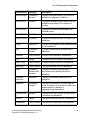
Family Name Product Name Manual Type, version W-2004.12
iii
iv
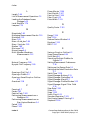
Table Of Contents
Chapter 1.
Introduction ................................................................................1-1
Invoking CosmosScope................................................................................1-2
Command Line Invocation and Options ....................................................1-2
Opening a Plot File......................................................................................1-3
Tutorials ......................................................................................................1-3
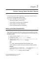
Chapter 2.
Tutorial: Viewing Saber Simulator Results ..............................2-1
Setting up the Saber Simulator Data ........................................................2-1
Viewing Saber Transient Analysis Waveforms..........................................2-2
Viewing Saber AC Analysis Waveforms.....................................................2-3
Performing Measurements on a Waveform................................................2-4
Chapter 3.
Tutorial: Viewing HSPICE Results ...........................................3-1
Setting up the Design Data ........................................................................3-1
Viewing HSPICE Transient Analysis Waveforms.....................................3-2
Viewing AC Analysis Waveforms ...............................................................3-3
Performing Measurements on an HSPICE Waveform ..............................3-4
Chapter 4.
CosmosScope Menus Reference ................................................. 4-1
File Pulldown Menu Options ......................................................................4-1
File>New ................................................................................................4-2
File>Open ...............................................................................................4-2
File>Close...............................................................................................4-2
File>Save................................................................................................4-2
File>Export Image .................................................................................4-3
File>Configuration.................................................................................4-3
CosmosScope Reference Manual (Dec. 2004)
Copyright © 1985-2004 Synopsys, Inc.
5
Table Of Contents
File>Print ...............................................................................................4-4
File>Printer............................................................................................4-4
File>Exit ......................................................................................................4-4
Edit Pulldown Menu Options .....................................................................4-4
Undo .......................................................................................................4-4
Cut, Copy, Paste, Delete ........................................................................4-4
Graph Preferences .................................................................................4-5
Graph Tab .........................................................................................4-5
Signal Tab .........................................................................................4-6
Display Tab .......................................................................................4-6
XY Tab...............................................................................................4-8
Scope Preferences ................................................................................4-10
Reader Tab ......................................................................................4-10
Signal Manager Tab .......................................................................4-10
Measurement Tab...........................................................................4-11
Graph Pulldown Menu Options................................................................4-12
Plot........................................................................................................4-12
Paste .....................................................................................................4-12
Graph>Annotate Info Menu Option.................................................... 4-12
Graph>Zoom Menu Options ................................................................4-12
Graph>Signal Attributes Menu Option..............................................4-13
Signal Attributes - View Axis Options .......................................... 4-16
Vertical Axis Options 4-16
Horizontal Axis Options 4-16
Graph>Axis Attributes Menu Option ................................................. 4-18
Graph>Members Menu Option ...........................................................4-21
Graph>Measure Results Menu Option............................................... 4-23
Graph>Waveform Compare Menu Option.......................................... 4-26
Graph>Signal Search Menu Option.................................................... 4-26
Graph>Selected Axes Menu Option.................................................... 4-26
Range...............................................................................................4-26
Scale ................................................................................................4-27
Grids................................................................................................4-27
Sliders .............................................................................................4-27
6
CosmosScope Reference Manual (Dec. 2004)
Copyright © 1985-2004 Synopsys, Inc.
Table Of Contents
Lock Menu Item..............................................................................4-28
Graph>Selected Signals Menu Option ............................................... 4-29
Selected Signals>Stack Region Menu Item .................................. 4-29
Selected Signals>Color Menu Item ............................................... 4-30
Selected Signals>Style Menu Item................................................4-30
Selected Signals>Line Width ......................................................... 4-30
Selected Signals>Symbol Menu Item ............................................ 4-31
Selected Signals>Symbol Size Menu Item .................................... 4-31
Selected Signals>View Menu Item ................................................4-31
Selected Signals>Signal Grid Menu Item ..................................... 4-31
Selected Signals>Trace Height Menu Item .................................. 4-32
Selected Signals>Digital Display Menu Item ............................... 4-32
Selected Signals>Create Bus Menu Item......................................4-32
Selected Signals > Convert To Digital...........................................4-33
Selected Signals > Delete Signals Menu Item ..............................4-33
Graph>Selected Graphics Menu Option.............................................4-34
Graph>Font Menu Option ...................................................................4-34
Graph>Color Map Menu Option ......................................................... 4-34
Graph>Legend Menu Option ..............................................................4-34
Graph>Match Aspect Ration Menu Option........................................4-35
Graph>Rename Window Title Menu Option......................................4-35
Graph>Clear Graph.............................................................................4-35
Tools Pulldown Menu Options..................................................................4-35
Window Pulldown Menu Options .............................................................4-35
Help Pulldown Menu Options ..................................................................4-36
CosmosScope Popup Menus ......................................................................4-36
Trace Popup Menu ...............................................................................4-37
Graph Popup Menu..............................................................................4-37
Axis Popup Menu .................................................................................4-39
Signal Popup Menu..............................................................................4-39
Measure Popup Menu ..........................................................................4-40
AimDraw Popup Menu ........................................................................4-41
Chapter 5.
Signal Manager ..........................................................................5-1
CosmosScope Reference Manual (Dec. 2004)
Copyright © 1985-2004 Synopsys, Inc.
7
Table Of Contents
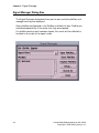
Accessing the Signal Manager....................................................................5-2
Opening a Plotfile........................................................................................5-2
HSPICE Sweep Filtering ...........................................................................5-3
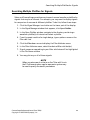
Searching Multiple Plotfiles for Signals ....................................................5-5
Signal Manager Dialog Box ........................................................................5-6
Signal Manager Menus ...............................................................................5-7
Signal Manager File Menu Items .........................................................5-7
Signal Manager Plotfile Menu .........................................................5-7
Signal Manager Signals Menu Items ..............................................5-8
Signal Manager Signal Filter Field..........................................................5-10
Signal Manager Buttons ...........................................................................5-11
Signal Manager Setup Button Dialog Box .........................................5-11
Signal Manager Plotfile Window ..............................................................5-13
Plotfiles Dialog Box Menus..................................................................5-14
Plotfiles Dialog Box Fields...................................................................5-15
Plotfiles Dialog Box Use Notes............................................................5-16
Chapter 6.
Graph Window Operation ..........................................................6-1
Displaying a Graph .....................................................................................6-2
Saving a Graph or Outline..........................................................................6-2
Opening a Saved Graph or Outline ............................................................6-3
Redraw Status Window...............................................................................6-4
Zooming........................................................................................................6-5
Zooming In..............................................................................................6-5
Zooming Out...........................................................................................6-5
Zooming to Fit ........................................................................................6-6
Panning ........................................................................................................6-7
Scroll Bars ...................................................................................................6-8
Slider............................................................................................................6-8
Trace Graph Region ....................................................................................6-9
Analog Graph Region ................................................................................6-10
Smith Chart...............................................................................................6-11
Polar Chart ................................................................................................6-12
Chapter 7.
8
Measurement Tool ......................................................................7-1
CosmosScope Reference Manual (Dec. 2004)
Copyright © 1985-2004 Synopsys, Inc.
Table Of Contents
Accessing the Measurement Tool ...............................................................7-2
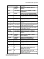
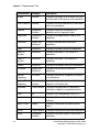
List of Measurement Operations................................................................7-2
How to Use the Measurement Tool ............................................................7-6
Measurement Dialog Box ......................................................................7-6
Selecting a Measurement ......................................................................7-7
Selecting a Signal for a Measurement ..................................................7-7
Setting the Range of a Measurement ...................................................7-8
Creating a New Waveform of Measurement Results ...........................7-8
Managing Measurement Results..............................................................7-10
Accessing the Measurement Results Dialog Box ............................... 7-10
Measurement List................................................................................7-11
Status List ............................................................................................7-12
Signal Field ..........................................................................................7-12
Multi-Member Waveform Measurements ................................................7-12
Multi-Member Count ...........................................................................7-15
Multi-Member Count Example ...........................................................7-16
Setting Measurement Preferences ...........................................................7-18
Topline/Baseline Calculation ....................................................................7-20
Manually Set a Custom Topline/Baseline .......................................... 7-21
Default Calculation..............................................................................7-21
Waveform Reference Levels ......................................................................7-23
AC Coupled RMS.......................................................................................7-25
Amplitude ..................................................................................................7-26
At X ............................................................................................................7-27
Average ......................................................................................................7-29
Bandwidth .................................................................................................7-30
Baseline .....................................................................................................7-33
Cpk .............................................................................................................7-34
Crossing .....................................................................................................7-35
Damping Ratio...........................................................................................7-38
dB ...............................................................................................................7-39
Delay ..........................................................................................................7-40
Delta X .......................................................................................................7-42
Delta Y .......................................................................................................7-44
CosmosScope Reference Manual (Dec. 2004)
Copyright © 1985-2004 Synopsys, Inc.
9
Table Of Contents
Dpu.............................................................................................................7-45
Duty Cycle .................................................................................................7-46
Eye Diagram..............................................................................................7-48
Eye Mask ...................................................................................................7-52
Falltime ......................................................................................................7-55
Frequency ..................................................................................................7-57
Gain Margin ..............................................................................................7-58
Highpass ....................................................................................................7-59
Histogram ..................................................................................................7-61
Horizontal Level ........................................................................................7-62
Imaginary ..................................................................................................7-63
IP2 ..............................................................................................................7-64
IP3/SFDR ...................................................................................................7-69
Length ........................................................................................................7-74
Local Max/Min...........................................................................................7-76
Lowpass .....................................................................................................7-79
Magnitude..................................................................................................7-80
Maximum...................................................................................................7-81
Mean ..........................................................................................................7-83
Mean +3 std_dev........................................................................................7-84
Mean -3 std_dev.........................................................................................7-85
Median .......................................................................................................7-86
Minimum ...................................................................................................7-87
Natural Frequency ....................................................................................7-88
Nyquist Plot Frequency ............................................................................7-89
Overshoot...................................................................................................7-90
Pareto .........................................................................................................7-93
P1dB Measurement...................................................................................7-97
Peak-to-Peak............................................................................................7-102
Period .......................................................................................................7-103
Phase........................................................................................................7-105
Phase Margin...........................................................................................7-106
Point Marker............................................................................................7-107
Point to Point ...........................................................................................7-109
10
CosmosScope Reference Manual (Dec. 2004)
Copyright © 1985-2004 Synopsys, Inc.
Table Of Contents
Pulse Width .............................................................................................7-111
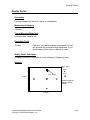
Quality Factor..........................................................................................7-113
Range .......................................................................................................7-114
Real ..........................................................................................................7-114
Risetime ...................................................................................................7-115
RMS..........................................................................................................7-117
Settle Time ..............................................................................................7-118
Slew Rate .................................................................................................7-120
Slope.........................................................................................................7-122
Standard Deviation .................................................................................7-123
Stopband ..................................................................................................7-124
Threshold (at Y).......................................................................................7-126
Topline .....................................................................................................7-127
Undershoot ..............................................................................................7-127
Vertical Level...........................................................................................7-129
Vertical Cursor ........................................................................................7-129
X at Maximum.........................................................................................7-130
X at Minimum .........................................................................................7-131
Yield .........................................................................................................7-132
Chapter 8.
RF Tool ........................................................................................8-1
Invoking the RF Tool...................................................................................8-1
Point Trace Measurements .........................................................................8-1
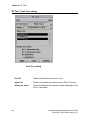
RF Tool - Point Trace dialog .................................................................8-2
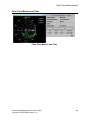
Point Trace Markers and Table ............................................................8-3
Noise Circle..................................................................................................8-4
Stability Circle.............................................................................................8-5
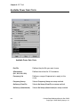
Available Power Gain Circle .......................................................................8-6
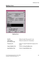
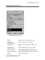
Operating Power Gain Circle......................................................................8-7
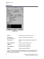
VSWR Circle ................................................................................................8-8
Parameter Conversion ................................................................................8-9
Conversion Procedure............................................................................8-9
Conversion Equations..........................................................................8-10
Chapter 9.
CosmosScope Quick Reference ..................................................9-1
CosmosScope Reference Manual (Dec. 2004)
Copyright © 1985-2004 Synopsys, Inc.
11
Table Of Contents
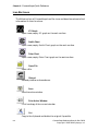
Icon Bar Icons..............................................................................................9-2
Tool Bar Icons ..............................................................................................9-5
Mouse Usage................................................................................................9-6
Hot Keys ......................................................................................................9-8
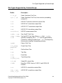
File Types Supported by CosmosScope ......................................................9-9
Chapter 10. External Waveform Database API ........................................... A-1
Creating a Database Reader...................................................................... A-1
Define Initialization Routine................................................................ A-2
Create Member Routines...................................................................... A-2
GetFormatAttProc ........................................................................... A-3
OpenContainerProc ......................................................................... A-3
CloseContainerProc ......................................................................... A-4
GetContainerAttProc....................................................................... A-4
GetWaveformAttProc....................................................................... A-4
CreateWaveformProc....................................................................... A-5
Waveform Creation Routines ............................................................... A-5
Non-parameterized Waveform Routine.......................................... A-6
WfX_Create() A-7
Wf_CreateDgt() A-8
WfX_AddValue() A-8
Wf_AddValues() A-9
Parameterized Waveform Routine................................................ A-10
WfX_AddNumberParameter() A-12
WfX_AddSetParameter() A-13
WfX_AddStringParameter() A-13
WfX_NextParameterValue() A-13
Compiling and Linking the Database Access Package (dll)................... A-14
Loading the Database Access Package.................................................... A-15
Files Provided with the Saber Software.................................................. A-16
Chapter 11. ASCII File Export and Import .................................................. B-1
Export ......................................................................................................... B-1
Set Export Preferences ......................................................................... B-1
Exporting Waveforms ........................................................................... B-1
Exporting Plotfiles ................................................................................ B-2
12
CosmosScope Reference Manual (Dec. 2004)
Copyright © 1985-2004 Synopsys, Inc.
Table Of Contents
Import ......................................................................................................... B-2
Waveform Descriptor / Header: ............................................................ B-3
Independent variable element: ....................................................... B-3
Dependent variable element: .......................................................... B-3
Data............................................................................................................. B-4
Sample ASCII Import File ......................................................................... B-4
Index ......................................................................................................... Index-1
Bookshelf ............................................................................................Bookshelf-1
CosmosScope Reference Manual (Dec. 2004)
Copyright © 1985-2004 Synopsys, Inc.
13
Table Of Contents
14
CosmosScope Reference Manual (Dec. 2004)
Copyright © 1985-2004 Synopsys, Inc.
Chapter
1
Introduction
CosmosScope is a graphical waveform analyzer tool that allows you to view
and analyze simulation results in the form of waveforms displayed on graphs,
or as values displayed in lists. Tools available with CosmosScope include:
• the Signal Manager, through which the plotfiles are opened, filtered,
and placed into a graph window or calculator
• the Measurement Tool, which provides over 50 measurements that can
be applied to a waveform
• the Waveform Calculator, which emulates a hand-held calculator that
interacts graphically with the application
• the Command Line Tool, which allows you to enter AIM commands,
write scripts, and save them into files
CosmosScope Reference Manual (Dec. 2004)
Copyright © 1985-2004 Synopsys, Inc.
1-1
Chapter 1: Introduction
Invoking CosmosScope
There are a number of different ways to invoke Scope, including:
• On a Windows system, use the command line invocation described
below, or simply select:
Programs > {install_location} > Scope
or
Programs > {install_location} > CosmosScope
• To invoke the product on UNIX systems, see the command line
invocation instructions, below.
Command Line Invocation and Options
CosmosScope can be executed from the UNIX command prompt or from the
Command Prompt window. The full form of the scope and cscope commands
for CosmosScope is shown below:
cscope [-h][-display host[:server.display]]
[-pfiles pfilename][pfile...]][-noconfig][-geom geom]
[-script aimfile
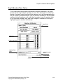
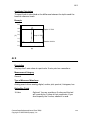
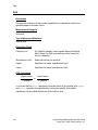
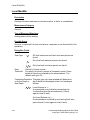
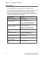
The following table describes the scope and cscope command options.
1-2
Option
Description
-h
Displays the scope (or cscope) command syntax and
a list of the invocation options.
-display host:0.0
Displays screen graphics on the specified host. On
some systems, you can replace host:0.0 with
unix:0.0 or:0.0, when the display host is the one
running the simulator (or the Scope Waveform
Analyzer).
-pfiles pfile
Specifies the plotfile to be opened at start-up.
-noconfig
Requests that the saved configuration not be loaded on
start-up.
-geom geom
Defines the geometry for the Scope window.
-script aimfile
Executes the specified AIM script on start-up.
CosmosScope Reference Manual (Dec. 2004)
Copyright © 1985-2004 Synopsys, Inc.
Opening a Plot File
Option
Description
-app application name Specifies the application that CosmosScope is
integrated with. The value can be saber, cosmos, or
saberhdl.
Opening a Plot File
To open a plot file:
• Choose the File > Open... > Plotfile... menu choice. This choice displays
the Open Plot Files dialog box.
• In the Directory field, navigate to the directory that contains the plot file
you wish to analyze.
• Set the Files of type field as appropriate for the kind of plot file you wish
to open.
• Highlight the desired file and click the Open button. Refer to the
information on the Signal Manager tool to begin your analysis.
Tutorials
The following topics provide tutorials on how to use CosmosScope to view
different waveforms:
• Tutorial: Viewing Saber Simulator Results
• Tutorial: Viewing HSPICE Results
CosmosScope also reads AWD, FSDB Version 2.3 (EPIC, VERILOG), VCD,
TouchStone, Star-SimXT and Polaris plot files. While these output formats are
not covered in these tutorials, the process of opening these files and using
CosmosScope with them is similar to the process shown in these tutorials.
CosmosScope Reference Manual (Dec. 2004)
Copyright © 1985-2004 Synopsys, Inc.
1-3
Chapter 1: Introduction
1-4
CosmosScope Reference Manual (Dec. 2004)
Copyright © 1985-2004 Synopsys, Inc.
Chapter
2
Tutorial: Viewing Saber Simulator Results
In this tutorial you will use CosmosScope to view analysis results from the
simulation of a single-stage amplifier design.
This tutorial is divided into the following topics:
• Setting up the Saber Simulator Data
• Viewing Saber Transient Analysis Waveforms
• Viewing Saber AC Analysis Waveforms
• Performing Measurements on a Waveform
Setting up the Saber Simulator Data
Saber Simulator analysis results for a simple transistor amplifier have been
provided for use with this tutorial. Create a directory and make a copy of the
example as follows:
1. Create a directory called synopsys_tutorial.
2. Navigate to the new synopsys_tutorial directory.
3. Copy the install_home/examples/Saber/SaberScope/saber_amp
directory to the synopsys_tutorial directory:
UNIX:
cp -r install_home/examples/Saber/SaberScope/saber_amp .
install_home is the location where your software has been installed.
Windows:
In Windows Explorer, hold down the Ctrl key and drag the saber_amp
folder from \examples\Saber\SaberScope\ to the
synopsys_tutorial directory you just created.
CosmosScope Reference Manual (Dec. 2004)
Copyright © 1985-2004 Synopsys, Inc.
2-1
Chapter 2: Tutorial: Viewing Saber Simulator Results
Viewing Saber Transient Analysis Waveforms
The results of a Saber Simulator transient analysis reside in the saber_amp
directory. You can view the results with the CosmosScope Waveform Analyzer
as follows:
1. Invoke CosmosScope.
2. Open the Open Plotfiles dialog box: File > Open > Plotfiles.
3. In the Open Plotfiles dialog box, browse to the
synopsys_tutorial\saber_amp directory; in the Files of type field,
select Saber pl (*.ai_pl, *.p1, *.p1*).
4. Click on the single_amp.tr.ai_pl item and click the Open button.
The Signal Manager and the single_amp.tr.ai_pl Plot File windows are
displayed.
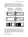
5. From the single_amp.tr.ai_pl Plot File window, select signal in by
left-clicking it. The signal is highlighted.
6. Plot the selected signal on the graph by clicking the Plot button.
7. In the single_amp.tr.ai_pl Plot File window, select signal aout.
8. Plot the selected signal on the same graph as the in signal by moving
the cursor to the Graph window and clicking the middle mouse button.
When using a two-button mouse, place the cursor in the graph region,
click the right mouse button to bring up the graph pop-up, then select
Plot.
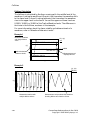
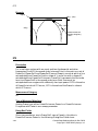
These waveforms show the input and the output of a simple transistor
amplifier.
9. Zoom in to the area between 2u and 4u by moving the cursor to the
X-axis 2u tick mark.
10. Click-and-hold the left mouse button and drag it over to the 4u tick
mark and release the button. The same technique can be used to zoom
on the Y-axis.
11. If you like, experiment with the Zoom icons
.
12. When you have finished viewing the waveforms, click the Clear icon
2- 2
.
CosmosScope Reference Manual (Dec. 2004)
Copyright © 1985-2004 Synopsys, Inc.
Viewing Saber AC Analysis Waveforms
Viewing Saber AC Analysis Waveforms
The results of a Saber Simulator AC analysis also reside in the saber_amp
directory. You can view these results as follows:
1. In the Signal Manager dialog box, click on the Open Plotfiles button.
2. In the Open Plotfiles dialog box, click on the single_amp.ac.ai_pl
selection and click the Open button. The single_amp.ac.ai_pl Plot File
window is displayed.
3. In the single_amp.ac.ai_pl Plot File window, select signal aout and plot
it.
4. In this tutorial you do not need the Phase(deg):f(Hz) waveform. To
delete it from the Graph window, do the following:
a. Move the mouse cursor to the aout signal name associated with the
Phase(deg):f(Hz) plot. The aout signal name and the waveform
change color.
b. Press-and-hold the right mouse button to bring up the Signal Menu.
c. Select the Delete Signal item.
5. Do the following to see how you can plot additional waveforms to the
Graph window:
a. From the single_amp.tr.ai_pl Plot File window, plot the aout and in
signals. Two new waveforms are added to the graph window.
b. Delete the in and aout waveforms when you have finished viewing
them.
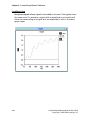
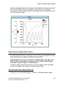
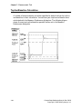
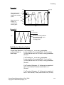
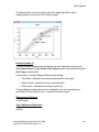
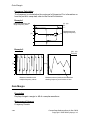
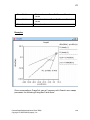
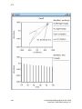
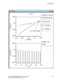
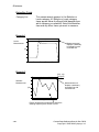
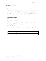
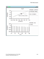
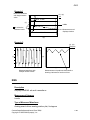
6. Look at the aout dB(V):f(Hz) (dB in volts versus frequency in Hertz)
waveform in the Graph window.
From the waveform you can see that the gain is about 10dB from about
2000 Hz to 300 kHz. The next part of this tutorial uses the
Measurement Tool on this waveform to get some accurate readings on
the gain and the frequency response.
CosmosScope Reference Manual (Dec. 2004)
Copyright © 1985-2004 Synopsys, Inc.
2-3
Chapter 2: Tutorial: Viewing Saber Simulator Results
Performing Measurements on a Waveform
The Measurement Tool allows you to perform various measurements on a
waveform. Check the bandwidth and gain of the single-stage amplifier output
signal (aout) as follows:
1. Use the Close buttons on the Plot File windows and the Signal Manager
dialog box to close them.
2. In the Tool Bar located at the bottom of
the CosmosScope window, click the Measurement icon
.
The Measurement dialog box appears.
3. Select the Bandwidth measurement in the Measurement dialog box as
follows:
a. Move the mouse cursor to the right of the Measurement field and
press and hold the left mouse button on the down arrow
button.
b. Move the mouse cursor down to the Frequency Domain menu.
c. Select Bandwidth.
To summarize, choose the Measurement >
Frequency Domain > Bandwidth menu item.
2- 4
CosmosScope Reference Manual (Dec. 2004)
Copyright © 1985-2004 Synopsys, Inc.
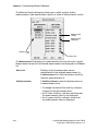
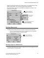
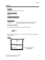
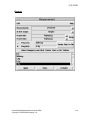
Performing Measurements on a Waveform
d. Because there is only one signal in the Graph window, aout should
appear in the Signal field in the Measurement dialog box as shown in
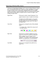
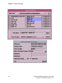
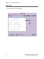
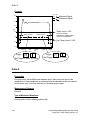
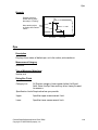
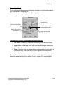
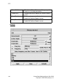
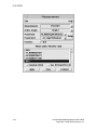
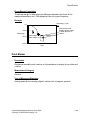
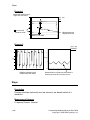
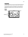
the following figure.
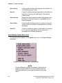
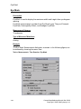
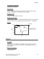
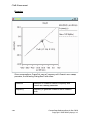
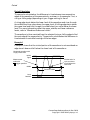
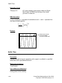
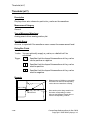
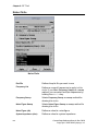
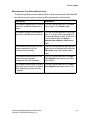
Measurement = Bandwidth
Signal = aout
Click these buttons to
display levels on graph.
Click them again to hide
the values.
e. If you want to see values displayed on the graph for Topline and
Offset that are used in the bandwidth calculation, click the visibility
indicator buttons to the right of the Reference Levels fields they will
turn green to indicate they’re activated.
f. Click the Apply button. The bandwidth is displayed on the graph.
4. Select the Gain Margin measurement by doing the following:
a. Choose the Measurement > Frequency Domain > Gain Margin menu
item.
b. Click the Apply button. The gain margin is displayed on the graph.
c. You can select the measurement labels and move them if the graph
becomes too cluttered. Position the cursor over the text. Then
left-click and hold while moving the cursor to a new location.
5. You can get more information about each of the measures you
performed or control the amount of information displayed in the Graph
window by using the Measure Results dialog box as follows:
CosmosScope Reference Manual (Dec. 2004)
Copyright © 1985-2004 Synopsys, Inc.
2-5
Chapter 2: Tutorial: Viewing Saber Simulator Results
a. In the Graph window, move the mouse cursor to the aout signal
name.
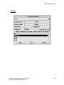
b. Use the popup menu and choose the Signal Menu > Measure Results...
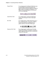
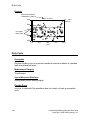
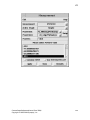
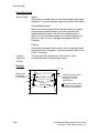
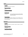
item. A Measure Results dialog box appears.
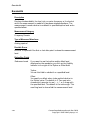
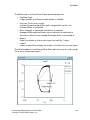
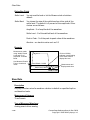
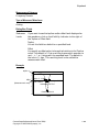
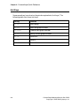
c. In the Measure Results dialog box, be sure the Bandwidth item in the
left column is selected as shown in the following figure:
Visibility
Indicators
Select button
Click these buttons to
display levels on graph.
Click them again to hide
the values.
d. Notice in the Measure Results dialog box, in the right column, the
different values that are available from executing the bandwidth
measurement.
e. Click on the various visibility indicators to choose which values are
displayed in the Graph window.
f. When you have finished exploring the Measure Results dialog box,
close it.
6. To close CosmosScope, select the File > Exit menu item.
This concludes the tutorial for analyzing Saber Simulator results.
2- 6
CosmosScope Reference Manual (Dec. 2004)
Copyright © 1985-2004 Synopsys, Inc.
Chapter
3
Tutorial: Viewing HSPICE Results
In this tutorial you use CosmosScope to view the analysis results from the
simulation of a single-stage amplifier design.
This tutorial is divided into the following topics:
• Setting up the Design Data
• Viewing HSPICE Transient Analysis Waveforms
• Viewing AC Analysis Waveforms
• Performing Measurements on a HSPICE Waveform
Setting up the Design Data
Analysis-results from a simple transistor amplifier have been created for you
using the HSPICE transient and AC simulators for use with this tutorial. You
will create a directory and then make a copy of the example as follows:
1. Create a directory called synopsys_tutorial.
2. Navigate to the new synopsys_tutorial directory.
3. Copy the install_home/examples/Saber/CScope/hspice_amp
directory to the synopsys_tutorial directory:
UNIX:
cp -r install_home/examples/Saber/CScope/hspice_amp
install_home is the location where your software has been installed.
Windows:
In Explorer, hold down the Ctrl key and drag the hspice_amp folder
from install_home\examples\Saber\CScope\ to the
synopsys_tutorial directory that you just created.
CosmosScope Reference Manual (Dec. 2004)
Copyright © 1985-2004 Synopsys, Inc.
3-1
Chapter 3: Tutorial: Viewing HSPICE Results
Viewing HSPICE Transient Analysis Waveforms
The results of a simulator transient analysis reside in the hspice_amp
directory. You can view the results with the CosmosScope Waveform Analyzer
as follows:
1. Invoke CosmosScope.
2. Open the Open Plotfiles dialog box: File > Open > Plotfiles.
3. In the Open Plotfiles dialog box, browse to the
synopsys_tutorial\hspice_amp directory; in the Files of type field,
select HSPICE (*.tr*, *.ac*, *.sw*, *.ft*) item.
4. Click on the amp.tr0 item and click the Open button. The Signal
Manager and the amp Plot File windows are displayed.
5. From the amp Plot File window, select signal v(in) by left-clicking it.
The signal is highlighted.
6. Plot the selected signal on the graph by clicking the Plot button.
7. In the amp Plot File window, select signal v(aout).
8. Plot the selected signal on the same graph as the v(in) signal by
moving the cursor to the Graph window and clicking the middle mouse
button. When using a two-button mouse, place the cursor in the graph
region, click the right mouse button to bring up the graph pop-up, then
select Plot.
These waveforms show the input and the output of a simple transistor
amplifier.
9. Zoom in to the area between 2u and 4u by moving the cursor to the
X-axis 2u tick mark.
10. Click-and-hold the left mouse button and drag it over to the 4u tick
mark and release the button. The same technique can be used to zoom
on the Y-axis.
11. If you like, experiment with the Zoom icons
.
12. When you have finished viewing the waveforms, click the Clear icon
3-2
.
CosmosScope Reference Manual (Dec. 2004)
Copyright © 1985-2004 Synopsys, Inc.
Viewing AC Analysis Waveforms
Viewing AC Analysis Waveforms
The results of a simulator AC analysis also reside in the hspice_amp
directory. You can view these results as follows:
1. In the Signal Manager dialog box, click on the Open Plotfiles button.
2. In the Open Plotfiles dialog box, in the Files of type field, select the
HSPICE (*.tr*, *.ac*, *.sw*, *.ft*) item.
3. Click on the a.ac0 selection and click the Open button. The “a” Plot File
window is displayed.
4. In the Plot File window, select signal v(aout) and plot it.
5. In this tutorial you do not need the Phase(deg):Frequency(Hertz)
waveform. To delete it from the Graph window, do the following:
a. Move the mouse cursor to the v(aout) signal name associated with
the Phase plot. The v(aout) signal name and the waveform change
color.
b. Press-and-hold the right mouse button to bring up the Signal Menu.
c. Select the Delete Signal item.
6. Change the X-axis attributes to display as a logarithmic waveform as
follows:
a. To bring up the Axis Menu, move the cursor to the X-axis and
click-and-hold the right mouse button.
b. To bring up the Axis Attributes dialog box, select the Attributes menu
item.
c. In the Scale field, click the Log radio button. The waveform should
now look similar to a bell curve.
d. Close the Axis Attributes dialog box.
7. Do the following to see how you can plot additional waveforms to the
Graph window:
a. From the amp Plot File window, plot the v(aout) and v(in)
signals. Two new waveforms are added to the graph window.
b. When you have finished viewing the v(in) and v(aout) waveforms
that you just plotted in the previous step, delete them as follows:
First move the cursor to the waveform name on the graph. Then
select the Signal Menu > Delete Signal menu item by right-clicking the
mouse button. Do this for each signal you want to delete.
CosmosScope Reference Manual (Dec. 2004)
Copyright © 1985-2004 Synopsys, Inc.
3-3
Chapter 3: Tutorial: Viewing HSPICE Results
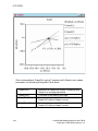
8. Look at the vdb(aout) dB(V):Frequency(Hertz) waveform in the
Graph window.
From the waveform you can see that the gain is about 10dB from about
2000 Hz to 300 kHz. The next part of this tutorial uses the
Measurement Tool on this waveform to get some accurate readings on
the gain and the frequency response.
Performing Measurements on an HSPICE Waveform
The Measurement Tool within CosmosScope provides a method of performing
various measurements on a waveform. You check the bandwidth and gain of
the single-stage amplifier output signal v(aout) as follows:
1. Close the Plot File windows and the Signal Manager window.
2. In the Tool Bar located at the bottom of
the CosmosScope window, click the Measurement icon
.
The Measurement dialog box appears.
3. Select the Bandwidth measurement in the Measurement dialog box as
follows:
a. Move the mouse cursor to the right of the Measurement field and
press and hold the left mouse button on the down arrow
button.
b. Move the mouse cursor down to the Frequency Domain menu.
c. Select Bandwidth.
To summarize, choose the Measurement >
Frequency Domain > Bandwidth menu item.
3-4
CosmosScope Reference Manual (Dec. 2004)
Copyright © 1985-2004 Synopsys, Inc.
Performing Measurements on an HSPICE Waveform
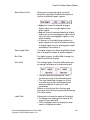
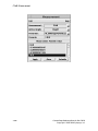
d. Because there is only one signal in the Graph window, v(aout)
should appear in the Signal field in the Measurement dialog box as
shown in the following figure.
Measurement = Bandwidth
Signal = v(aout)
Click these buttons to
display levels on graph.
Click them again to hide
the values.
e. If you want to see values displayed on the graph for Topline and
Offset that are used in the bandwidth calculation, click the visibility
indicator buttons to the right of the perspective Reference Levels
fields.
f. Click the Apply button. The bandwidth is displayed on the graph.
4. Select the Gain Margin measurement by doing the following:
a. Choose the Measurement > Frequency Domain > Gain Margin menu
item.
b. Click the Apply button. The gain margin is displayed on the graph.
c. You can select the measurement labels and move them if the graph
becomes too cluttered. Position the cursor over the text. Then
left-click and hold while moving the cursor to a new location.
CosmosScope Reference Manual (Dec. 2004)
Copyright © 1985-2004 Synopsys, Inc.
3-5
Chapter 3: Tutorial: Viewing HSPICE Results
5. You can get more information about each of the measures you
performed or control the amount of information displayed in the Graph
window by using the Measure Results dialog box:
a. In the Graph window, move the mouse cursor to the v(aout) signal
name.
b. Use the popup menu and choose the Signal Menu > Measure Results...
item. A Measure Results dialog box appears.
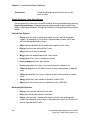
c. In the Measure Results dialog box, be sure the Bandwidth item in the
left column is selected (see the following figure).
Visibility
Indicators
Select button
Click these buttons to
display levels on graph.
Click them again to hide
the values.
d. Notice in the Measure Results dialog box, in the right column, the
different values that are available from executing the bandwidth
measurement.
e. Click on the various visibility indicators to choose which values are
displayed in the Graph window.
f. When you have finished exploring the Measure Results dialog box,
close it.
6. When you have finished trying out the features of CosmosScope, close
the application by selecting the File > Exit menu item.
3-6
CosmosScope Reference Manual (Dec. 2004)
Copyright © 1985-2004 Synopsys, Inc.
Performing Measurements on an HSPICE Waveform
This concludes the tutorial.
CosmosScope Reference Manual (Dec. 2004)
Copyright © 1985-2004 Synopsys, Inc.
3-7
Chapter 3: Tutorial: Viewing HSPICE Results
3-8
CosmosScope Reference Manual (Dec. 2004)
Copyright © 1985-2004 Synopsys, Inc.
Chapter
4
CosmosScope Menus Reference
This chapter provides reference information on each of the selections available
from the CosmosScope pulldown and popup menus:
• File Pulldown Menu Options
• Edit Pulldown Menu Options
• Undo
• Cut, Copy, Paste, Delete
• Graph Preferences
• Scope Preferences
• Graph Pulldown Menu Options
• Tools Pulldown Menu Options
• Window Pulldown Menu Options
• Help Pulldown Menu Options
• Popup Menus
Additional menus are associated with the Signal Manager Tool; these are
covered in the Signal Manager Chapter of this manual.
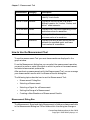
File Pulldown Menu Options
The File pulldown menu allows you to open existing files, save your work to
new files, create new windows, save configuration settings, open the print
dialog box, and exit the application.
CosmosScope Reference Manual (Dec. 2004)
Copyright © 1985-2004 Synopsys, Inc.
4-1
Chapter 4: CosmosScope Menus Reference
File>New
This option opens a new graph window formatted as an X-Y axis graph, a
Smith Chart graph, or a Polar Chart graph.
File>Open
This option allows you to open an existing plot file, graph, or outline using the
Open Files dialog box. Select the Files of Type from the pulldown list, and
browse to the location of the file you want to open.
File>Close
This option closes the active graph window or the current design.
File>Save
The Save Graph dialog box allows you to specify a path and file name. In
addition, a popup dialog box prompts you to save the graph file in one of the
following ways:
• With a copy of the waveforms in the graph.
• With a reference to the plot file from which the waveforms in the graph
were plotted.
In the first case, all connection to the plot file is lost. In the second case, the
connection to the plot is maintained. Thus, if the graph is reopened it can be
automatically updated due to any Replace or Append plot actions specified for
the plot file in an analysis.
The Save Outline dialog box allows you to specify a path and file name for an
outline. In addition, a Graph Outline popup dialog box allows you to specify
several attributes for the saved outline. You can select whether or not to
maintain the connection to the plot file in the same way as for a graph outline.
You control this by checking (or unchecking) the Dependencies checkbutton on
the Graph Outline dialog box.
The File > Save > Plotfile (*.txt) menu choice allows you to save the selected
waveforms into a text file.
4-2
CosmosScope Reference Manual (Dec. 2004)
Copyright © 1985-2004 Synopsys, Inc.
File Pulldown Menu Options
File>Export Image
This option opens an Export Image dialog box which allows you to export the
contents of an editor window to a file in a variety of graphics formats.
CosmosScope can create graphics files in the following formats:
PNG (*.png)
Portable Network Graphics
JPEG (*.jpg, *.jpeg)
TIFF (*.tiff, *.tif)
Tagged Interchange Format
XPM (*.xpm)
X-Window Pixel map
PCL5 (*.pcl5)
HPGL2 (*.hpgl2)
HP Graphics Language
Postscript (*.ps, *.eps)
AutoCad DXF (*.dxf)
CGM (*.cgm)
Computer Graphics Metafile
BMP (*.bmp)
PC Windows Bitmap
EMF (*.emf) in Windows NT only
Enhanced Metafile
File>Configuration
There are two options, and one setting, available.
• Save saves your work surface configuration immediately.
• Clear clears any saved configuration you have made in the current
session. The next time CosmosScope is invoked your configuration will
return to the default settings.
• Save on Exit checkbox setting saves your configuration settings upon
exiting CosmosScope. To do this, you must start the application from
the directory in which your work will be performed. The next time you
invoke CosmosScope, these settings will be retained.
• Save in working directory saves your work surface configuration into the
directory where CosmosScope has been invoked.
• Save in home directory saves your work surface configuration into your
home directory.
CosmosScope Reference Manual (Dec. 2004)
Copyright © 1985-2004 Synopsys, Inc.
4-3
Chapter 4: CosmosScope Menus Reference
When CosmosScope is invoked, it will try to load the configuration file,
.scopecfg, from the local directory. If it can’t find the file, it will try the home
directory.
File>Print
Select this option to open the Print dialog box. To print the current graph, single
click on the OK button.
File>Printer
This menu item appears in UNIX versions of CosmosScope. It allows you to
Create a new printer configuration, Remove a printer from the printer list, or
change the Properties of your printers.
File>Exit
This option closes the application.
Edit Pulldown Menu Options
Undo
Undo reverses any database operation you have just completed. This item does
not un-delete waveforms, undo measurement manipulations, operate on
general windows or UI operations. There is one level of undo. If the Undo
menu item is stippled or greyed out, it will not operate on your last action.
Cut, Copy, Paste, Delete
These menu options operate on the selected object.
• Cut removes a selected object and moves it into a clipboard.
• Copy copies a selected object in the active window into a clipboard.
• Paste will place whatever is in the clipboard into the active window.
• Delete will remove the currently selected items from the window.
4-4
CosmosScope Reference Manual (Dec. 2004)
Copyright © 1985-2004 Synopsys, Inc.
Edit Pulldown Menu Options
Graph Preferences
You may customize the appearance of your graphs, and modify other settings
by selecting Edit > Graph Preferences. This will bring up the Graph Preferences
window. Each tab in this window contains the following buttons:
• Apply new preferences to all graph windows immediately. This change
is good only for your current CosmosScope session unless you use the
Save button.
• To save your changes between CosmosScope sessions, click on the Save
button. You can now exit CosmosScope, return, and retain your new
preferences.
• The Defaults button sets your preferences to the original CosmosScope
default selections.
• The Reset button returns the work surface to the settings in place when
the current session was opened, or when the last settings were applied
with the Apply button.
• The Close button closes the dialog box and returns you to the work
surface.
Graph Tab
The Graph Tab allows you to change the colors and fonts used in your graphs.
You may specify color selections for Foreground, Highlight, Background 1, and
Background 2:
• Foreground consists of all displayed text, graph outlines, grids, and
markers.
• Highlight consists of text and signals, which are displayed as reverse
video when selected with the mouse cursor.
• Background 1 is the background of all of the graph regions.
• Background 2 is the background of the rest of the graph window.
To change colors:
• Single click on the colored square you want to change. A Color Editor
dialog box will be displayed, from which you may select or define new
custom colors. The reference material on the Drawing Tool provides
additional details on the Color Editor.
To change the style of text:
• Click on the ABC 123 button. The Font Selection dialog box will be
displayed to allow you to change the font settings.
CosmosScope Reference Manual (Dec. 2004)
Copyright © 1985-2004 Synopsys, Inc.
4-5
Chapter 4: CosmosScope Menus Reference
Signal Tab
Signals are the information displayed in the graphs. Each time you add
another analog signal, it is displayed in a different color. If your screen colors
are mapped to Mono, signals are displayed as a variety of dashed lines. These
dashed lines cannot be customized.
The Add button allows you to add more Signal Color fields.
The Delete button deletes the last Signal Color field.
To change signal colors:
• Single click on the buttons that contain the colored square. The Color
Editor dialog box will be displayed, from which you may select or define
new custom colors. The reference material on the Drawing Tool
provides additional details on the Color Editor.
For digital signals, CosmosScope displays different colors and line styles for
different logical states. Users can set the color and line style preferences with
this tab. Currently, CosmosScope supports logic_4, std_logic, and
nanosim_logic type digital signals.
Display Tab
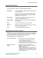
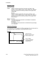
Legend Location Fields
The legend is the text that appears next to the
graph containing the labels of the axes and the
names of the displayed signals.
The legend can be configured to appear to the
right, bottom, left, or top of the graph, or it can
be configured as a floating legend.
Selecting the Float Button brings the legend up
in its own window. This window can be moved
anywhere within the graph window.
• To move the legend window, press and hold on
the legend window with the left mouse button.
• Drag the window to its new location and
release the mouse button.
4-6
CosmosScope Reference Manual (Dec. 2004)
Copyright © 1985-2004 Synopsys, Inc.
Edit Pulldown Menu Options
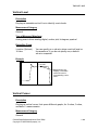
Grid Visibility Display
Default
The options to set the background grid
configuration are:
• Display - Specify whether to Hide or Show the
background grid. Default is "Hide."
• Line Style - Select solid, dashed or dotted grid
lines. Default is "Dashed".
• Line Width - Allows you to set the width of the
grid line. Default is "1."
• Line Color - Allows you to set the color of the
grid line. Default is "White."
Signal Name Default
When Leaf is selected, the signal name in the
legend will be displayed as the last text string
after the last slash when the signal name is a
long path name. When Full Path is selected, the
entire path name will be displayed.
Signal Line Width Default
Sets the default signal line width.
Default multi-member signal Sets the color mode for multi-member signals.
color display
In “Single Colored” mode, all the member curves
have the same color. In “Rainbow Colored”
mode, the member curves may have multiple
colors.
Dynamic Waveform Display Turn on the Dynamic Waveform Display feature
by clicking On and enter the interval, in
seconds, desired for continuously updating the
displayed waveform while a simulation is
continuing to run.
Open Dynamic Socket
Setting this to ON will allow updates to the
graph display via the socket from a simulator
running in debug mode.
Signal Highlight On
• Selecting the Waveform and legend button
allows you to put the mouse cursor on either
the signal displayed in the graph region or the
name of the signal in the legend in order to
highlight the signal. Mouse response is not as
quick as with the Legend only option.
• Selecting the Legend only button allows you to
put the mouse cursor on the name of the
signal in the legend in order to highlight the
signal. Mouse response is quicker than with
the Waveform and legend option.
CosmosScope Reference Manual (Dec. 2004)
Copyright © 1985-2004 Synopsys, Inc.
4-7
Chapter 4: CosmosScope Menus Reference
Signal Draw Feedback
Sets how often the Redraw Status window is
displayed. The default number of data points
before the Redraw Status window is displayed is
10,000. The higher the number of data points,
the fewer Redraw Status window updates are
displayed and the faster the window is redrawn.
XY Tab
Customizing specific to the XY type of graph is allowed through the XY Graph
Specific fields.
Digital Trace Height field
Changes the height of a digital signal in the
trace graph region.
Analog Trace Height field
Changes the height of an analog signal in the
trace graph region.
Bus Display Default buttons Change the base numeric value (radix) of the
value displayed in the trace graph region. This
option operates when digital signals are
combined into a bus.
Trace Snap buttons
Allow you to turn the trace snap for the digital
markers on or off. When On, the digital marker
will snap to the nearest state change. When Off,
the digital marker can be placed anywhere in
the digital graph.
Analog Paste Buttons
Select where new signals will be placed in the
graph window if they are not pasted into an
existing graph region.
• New signals can be placed in a separate, new,
graph region by selecting New Region.
• New signals can be placed in the trace graph
region by selecting Trace Region.
• New signals can be placed in the graph at the
bottom of the first graph region window by
selecting Bottom Region.
4-8
CosmosScope Reference Manual (Dec. 2004)
Copyright © 1985-2004 Synopsys, Inc.
Edit Pulldown Menu Options
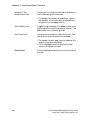
Axes Zoom
When you use the axes zoom feature using the
cursor, you can use this preference to either:
• Have the zoom display exactly where you
positioned the cursor zoom area (Exact
button).
• Have the zoom snap to the nearest tick marks
from the cursor-defined position (Nice Ticks
button). The grid increment definition
determines where the zoom will snap as
defined in the Axis Attributes dialog box, the
Grid Increment field.
Pre-Zoom X axis start and
end:
Allows you to set the zoom area of the X axis
prior to viewing a waveform. The default start
point of the zoom is set to start, which specifies
the start time of the simulation. The default end
point of the zoom is end, which specifies the last
point of the simulation.
You can specify relative positions to the start
and end point. For example, assume you have a
waveform covering a simulation time of 0u to
100u. You can specify start +20% end -20%
to cause the zoom to display the range from 20u
to 80u when the waveform is displayed.
You can specify a pre-zoom range using specific
constant values. Using the same waveform
example of 0u to 100u, if you put 20u as the
start point and 50u as the end point, the
waveform will display as zoomed in to that
range.
You can also specify relative positions using
constant values from the start and end point.
Again using a waveform that spans 0u to 100u,
if you specify a pre-zoom of start +20u end
-20u, the range from 20u to 80u appears when
the waveform is displayed.
Minimum Region Width
Minimum Region Height
Set the minimum size of a region. When
multiple signals are plotted in different regions,
the size of the region may be smaller than what
you want. These settings allows you to control
the minimum size.
CosmosScope Reference Manual (Dec. 2004)
Copyright © 1985-2004 Synopsys, Inc.
4-9
Chapter 4: CosmosScope Menus Reference
Default dB Scale
Sets the minimum and maximum values of the
dB view for signals. The dB view values could be
-Inf or Inf, if the original waveform contains 0 or
Inf data points. This setting makes the plot
easier to read.
Scope Preferences
Reader Tab
Default File Type
Allows you to select the default file type that
will be displayed when opening plotfiles. The
options reflect all the file types supported by
CosmosScope.
Saber PL Reader
Allows you to set the loading mode of the PL
reader.
Selecting “Incremental” makes the reader an
incremental reader - when a plot file is opened,
only the header for the plot will be read.
Selecting “Non-Incremental” makes the reader
a full reader - when a plot file is opened, the
whole data of the plot will be read.
Text Writer/Reader
“Writing Precision” allows you to set the
precsion of the data that will be written to the
text files.
“Name/Unit Separator” allows you to set the
separator between the waveform name, unit,
and type in the header of a text imput file. The
default separator is ‘.
Uncompressed Temporary Allows you to set the location of the temporary
Directory
directory used for opening gzipped files.
Signal Manager Tab
4-10
CosmosScope Reference Manual (Dec. 2004)
Copyright © 1985-2004 Synopsys, Inc.
Edit Pulldown Menu Options
This tab allows you to set the preferences for signal list windows. Please refer
to “Signal Manager Setup Button Dialog Box” in Chapter 5: Signal Manager”
for details.
Measurement Tab
This tab allows you to set the preferences for applying measurements. Please
refer to “Setting Measurement Preferences” in Chapter 7: Measurement Tool”
for details.
CosmosScope Reference Manual (Dec. 2004)
Copyright © 1985-2004 Synopsys, Inc.
4-11
Chapter 4: CosmosScope Menus Reference
Graph Pulldown Menu Options
Plot
This option allows you to plot selected signals from the signal list into the
graph region.
Paste
Places the contents of the clipboard into the graph region.
Graph>Annotate Info Menu Option
The Graph>Annotate Info menu option brings up a Text Variables dialog box,
which allows you to insert information into the graph window. The
information available is the current date, the creation date, and the author of
the current graph window.
To insert the current Date, Created date, and/or Author user id, click on the
adjacent Insert button to place the information on the graph. Once the text has
been placed into the graph window, you can move it around in the graph
window via drag and drop, or the annotations may be edited with the Draw
tool.
Graph>Zoom Menu Options
By selecting Zoom to Fit, the maximum number of data points will be displayed
on the graph, to show the entire range of a signal. All displayed graph regions
in the graph window are affected.
Zoom In increases magnification to show increased detail. All displayed graph
regions in the graph window are affected.
Zoom Out decreases magnification to show less detail, but more of the graphed
information. All displayed graph regions in the graph window are affected.
4-12
CosmosScope Reference Manual (Dec. 2004)
Copyright © 1985-2004 Synopsys, Inc.
Graph Pulldown Menu Options
Graph>Signal Attributes Menu Option
Selecting the Graph>Signal Attributes option opens the Signal Attributes dialog
box. This dialog box allows you to select any signal displayed in the graph
window, change the color of the signal, change the style of the line, add a
symbol to the signal, change the symbol width, fill the area under the signal,
manipulate the stack region, change the point of view of the signal, and
change the signal label.
Signal Field
Allows you to select a signal displayed in the
graph window to view or modify its attributes.
To display all available signals in the graph
window, single click the left mouse button on
the downward pointing arrow at the right of
the Signal field.
Color Field
Allows you to change the color of the selected
signal.
• To change colors, single click on any one of
the color buttons.
Style Field
Allows you to change the appearance of the
signal line. Several line styles are displayed.
Selecting None causes the signal line to
disappear. If the signal is also represented by
symbols, the symbols will still be displayed.
Line Width
Allows you to change the line width of the
signal line.
CosmosScope Reference Manual (Dec. 2004)
Copyright © 1985-2004 Synopsys, Inc.
4-13
Chapter 4: CosmosScope Menus Reference
4-14
Symbol Field
For analog signals, the Symbol field allows you
to add symbols to display the signal line.
Several symbol styles are displayed. Selecting
None causes the symbols to disappear. If the
signal is also represented by a line, the line
will still be displayed.
Symbol Size Field
For analog signals, the Symbol Width field
allows you to change the size of displayed
symbols.
Bar Field
For analog signals, the Bar field allows you to
fill in the area under a curve with a pattern.
Several bar patterns are displayed. The
pattern will be in the color of the signal.
Monotonic Plot Field
For analog signals, the Monotonic Plot field
allows you to display the signals in monotonic
mode, meaning, only points with interesting x
values will be plotted.
CosmosScope Reference Manual (Dec. 2004)
Copyright © 1985-2004 Synopsys, Inc.
Graph Pulldown Menu Options
Stack Region Field
Allows you to move the signal currently
selected in the Signal Attributes dialog box in
and out of different graph regions.
• Digital will move the selected analog or
digital signal into a single digital/trace
graph region.
• New will move the selected analog or digital
signal into a new analog graph region at the
top of all other analog graph regions in the
graph window.
• n (where n is the identifying number of a
graph region) will move the selected analog
or digital signal into the analog graph region
specified by the number n.
Trace Height Field
For digital signals, the Trace Height field allows
you to change the height of selected signals.
Bus Field
For digital signals, the Bus field changes the
digital information display.
View Field
For analog signals, the View fields allows you
to change the display of the selected signal.
• The left hand field changes the Y-axis
(vertical axis) plot of the selected signal.
• The right hand field changes the X-axis
(horizontal axis) plot of selected signals
based on different X-axis and Y-axis
parameters.
Details on the Vertical Axis Options and
Horizontal Axis Options are provided following
this table, below.
Label Field
Allows you to change the name of the signal.
• To change the name type the name of the
signal in the Label field.
• Click the Apply button to display the new
name in the graph window.
CosmosScope Reference Manual (Dec. 2004)
Copyright © 1985-2004 Synopsys, Inc.
4-15
Chapter 4: CosmosScope Menus Reference
Close Button
Closes the dialog box and returns you to the
work surface.
Signal Attributes - View Axis Options
Various options for the Vertical and Horizontal Axis are available by selecting
Graph>Signal Attributes; these options are implemented by setting the View:
fields in the Signal Attributes Dialog Box. Details on these options are provided
below.
Vertical Axis Options
• Real(x) uses the real X values of a signal as the Y-axis of the graph
region. For example, if the X-axis is represented in Hertz, the Y-axis
will also be represented in Hertz.
• dB(x) uses the decibels of the x value of a signal as the Y-axis .
• Real(y) plots the real value of the Y-axis.
• dB(y) plots the Y-axis in decibels.
• Mag(y) plots the magnitude of the Y-axis value.
• Imag(y) plots the Y-axis in imaginary terms.
• Phase(y) deg plots the Y-axis values .
• Phase(y) rad plots the Y-axis in terms of phase in radian units.
• CPhase(y) deg plots the Y-axis in terms of continuous phase, in degree
units.
• CPhase(y) rad plots the Y-axis in terms of continuous phase, in radian
units.
• dBm(y) plots the Y-axis values in decibels, times 1,000.
• dBu(y) plots the Y-axis values in decibels, times 1,000,000.
Horizontal Axis Options
• Real(x) plots the real value of the X-axis.
• dB(x) plots the X-axis values in decibels.
• Real(y) uses the real Y values of a signal as the X-axis of the graph
region. For example, if the Y-axis is represented in volts, the X-axis will
also be represented in volts.
4-16
CosmosScope Reference Manual (Dec. 2004)
Copyright © 1985-2004 Synopsys, Inc.
Graph Pulldown Menu Options
• dB(y) plots the X-axis in Y-axis terms and decibels. For example, if the
Y-axis is represented in volts, the X-axis will be represented in volts
and decibels.
• Mag(y) plots the magnitude of the Y-axis value.
• Imag(y) plots the X-axis in imaginary Y-axis terms. For example, if the
Y-axis is represented in volts, the X-axis will be represented in
imaginary volts.
• Phase(y) deg plots the X-axis in terms of phase, in degree units.
• Phase(y) rad plots the X-axis in terms of phase, in radian units.
• CPhase(y) deg plots the X-axis in terms of continuous phase, in degree
units.
• CPhase(y) rad plots the X-axis in terms of continuous phase, in radian
units.
• Real YvsX plots the signal with the Y-axis vertically and the X-axis
horizontally and in real terms.
• Real XvsY plots the signal with the X-axis vertically and the Y-axis
horizontally and in real terms.
• dBm(x) plots the X-axis values in decibels, times 1,000.
• dBu(x) plots the X-axis values in decibels, times 1,000,000.
CosmosScope Reference Manual (Dec. 2004)
Copyright © 1985-2004 Synopsys, Inc.
4-17
Chapter 4: CosmosScope Menus Reference
Graph>Axis Attributes Menu Option
This option opens the Axis Attributes dialog box. This dialog box allows you to
select an axis, zoom, pan, change the scale to linear or logarithmic, change
grid increments, toggle the axis grid, and edit the axis label.
Axis Field
Allows you to select and update any axis
displayed in the graph window. To display and
select an available axes from the graph window,
click the left mouse button on the down arrow to
the right of the Axis field.
Range Fields
These fields allow you to zoom and pan along
the axis associated with the Axis field. The field
of view is displayed in the Zoom From/To field.
The entire possible viewing range is displayed
beneath the Slider bar.
Zoom In Button
Allows you to increase magnification to show
increased detail.
Zoom to Fit Button
Allows you to display the maximum number
of data points to show the entire range of a
signal.
Zoom Out Button
Allows you to decrease magnification to show
less detail, but more of the graphed
information.
Zoom From/To Field
Displays the current field of view for the
selected axis and allows you to enter values for
the range you want to display.
• To change the field of view, type in the values
in the From/To fields and Single click on the
Apply button.
4-18
CosmosScope Reference Manual (Dec. 2004)
Copyright © 1985-2004 Synopsys, Inc.
Graph Pulldown Menu Options
Slider Bar
Allows you to pan along the selected axis.
• Press and hold the left mouse button and
move the slider bar right or left. The range
available to be displayed is shown below the
slider bar. The range displayed is dynamically
shown in the From/To field.
• Release the mouse button when the
coordinates you want are displayed in the
From/To field.
Unit Scale Factor
Allows you to set the unit prefix for axis labels.
For example, selecting ‘m’ will cause all labels to
be in “mili-” scale. The default is “auto,” and it
means not specified.
Scale Field
Toggles the selected axis scale. The Linear
button displays the selected axis scale in linear
increments. The Log button displays the
selected axis scale in logarithmic increments.
Increment Field (Grid,
Exponent)
Allows you to change the resolution of the axis
scale.
If you selected Linear for Scale, you will set the
Grid Increment. If you selected Log for Scale, you
will set Exponent Increment and Grids/Increment.
• Grid Increment -- Sets the unit difference
between labeled grids for a linear scale. For
example, inserting 20u for a time scale will
set each grid marking 20usec apart. This
setting is also used by the Nice Ticks option in
the Axes Zoom field of the Graph Preference
dialog box, the XY tab.
• Exponent Increment -- Sets the unit difference
between labeled grids for a log scale. For
example, inserting 1 for a frequency scale will
set each grid marking exponentially
apart—10, 100, 1000, etc.
• Grids/Increment -- Sets the number of
unlabeled subdivisions between grids for a log
scale.
CosmosScope Reference Manual (Dec. 2004)
Copyright © 1985-2004 Synopsys, Inc.
4-19
Chapter 4: CosmosScope Menus Reference
Number of Tick
Subdivisions Field
Allows you to change the number of gradations
(ticks) between grid increments.
• To change the number of gradations, type in
the number of ticks you want displayed and
single click on the Apply button.
Grid Visibility Field
Toggles the grid display. The Show button turns
the axis grid in the active graph window on. The
Hide button turns the axis grid off.
Axis Label Field
Allows you to change the label of the axis. The
actual units of the scale are not changed.
• To change the axis label type the name of the
signal in the Axis Label field.
• Click the Apply button to display the new
name in the graph window.
Close Button
4-20
Exits the dialog box and returns you to the work
surface.
CosmosScope Reference Manual (Dec. 2004)
Copyright © 1985-2004 Synopsys, Inc.
Graph Pulldown Menu Options
Graph>Members Menu Option
This Graph menu option opens the Member Attributes dialog box, if a graph
window containing multiple members is open. This allows you to control the
display of a signal consisting of multiple members, such as those generated by
Vary or Monte Carlo data analysis. You can show all members or an individual
member, hide all members or an individual member, show all member labels
or an individual member label, and loop through all members of the signal,
highlighting each member individually.
Signal Field
Label List
Visibility Indicators
Highlight Rate
Slider
Label Orientation
Buttons
Close Button
CosmosScope Reference Manual (Dec. 2004)
Copyright © 1985-2004 Synopsys, Inc.
4-21
Chapter 4: CosmosScope Menus Reference
Label List
Displays the label associated with each member of
a signal. Each label is associated with a visibility
indicator to the right in the dialog box.
Signal Field
Allows you to select any signal displayed in the
graph window.
• To display all available signals in the graph
window single click with the left mouse button on
the downward pointing arrow at the right of the
Signal field.
Visibility Indicator
Each Visibility Indicator shows the display status of
a member. Each indicator is associated with a
member label in the Label List to the left.
• To change the state of the visibility indicator,
single click with the left mouse button.
• An all black visibility indicator shows that
neither the label nor the member of the signal is
displayed.
• A half black and half green visibility indicator
indicates that the member of the signal, but not
the label, is displayed.
• An all green visibility indicator indicates that
both the label and the member of the signal are
displayed.
Color indicator
Each Color indicator shows the color of a member.
Clicking on it with the left mouse ubtton allows you
to change the member’s color.
Show All Members
Button
Displays all members of the signal shown in the
Signal field. No labels are displayed.
Show All Labels Button Displays all members, with labels, in the graph
window. The location of these labels can be
rearranged for ease of viewing.
• To move a label, press and hold the left mouse
button on a label you wish to move and move the
label.
• Release the mouse button to place the label.
4-22
CosmosScope Reference Manual (Dec. 2004)
Copyright © 1985-2004 Synopsys, Inc.
Graph Pulldown Menu Options
Hide All Button
Removes all members in the graph window from
view. Individual members can be displayed by
using the visibility indicators or all members can be
displayed by using the Show All Members button.
Loop Highlight Button
Sequentially highlights each member of a signal.
This button functions even if all members have
been hidden.
• To start or stop the loop, single click on the Loop
Highlight button
Single Colored Button
Sets the color mode of the multi-member wavefrom
to “single colored.” All the members will have the
same color.
Rainbow Colored button Sets the color mode of the multi-member wavefrom
to “rainbow colored.” The members may have
different colors.
Highlight Rate Slider
Regulates the rate of the Loop Highlight. When the
slider is set all the way to Slow there is a 5 second
delay between the highlight of members. The
resolution for control of the delay is in 50
millisecond increments.
Label Orientation
Buttons
Stack member labels from top to bottom or from left
to right.
Close Button
Closes the Member Attributes dialog box.
Graph>Measure Results Menu Option
CosmosScope Reference Manual (Dec. 2004)
Copyright © 1985-2004 Synopsys, Inc.
4-23
Chapter 4: CosmosScope Menus Reference
The Measure Results dialog box allows you to select a signal, delete
measurements, hide measurement results, or show all measurement results.
Measurement
Hidden
Measurement
Displayed
Measurement
List
Status List
The Measurement list displays all measurements that are active for a signal.
Measurement values for the selected measurement are displayed in the Status
list.
Status List
Displays a list of measurement values
associated with the selected measurement in
the Measurement list. Each value has a visibility
indicator associated with it.
Visibility Indicator
A Visibility Indicator shows the display status of
a measurement value.
• To change the state of the visibility indicator,
single click the left mouse button.
• An all black visibility indicator indicates that
the measurement value is not displayed.
• An all green visibility indicator shows that
the measurement value is displayed.
4-24
CosmosScope Reference Manual (Dec. 2004)
Copyright © 1985-2004 Synopsys, Inc.
Graph Pulldown Menu Options
Signal Field
Allows you to select any signal displayed in the
graph window.
To display all available signals in the graph
window, single click with the left mouse button
on the downward pointing arrow at the right of
the Signal field.
Select checkbox
The check boxes before the measurements are
used to select the measurements that you want
to export to a text report file.
Delete Measurement Button Permanently deletes the selected measurement.
Delete All Button
Permanently deletes all measurements for the
selected signal.
Show All Values Button
Displays all values for the selected
measurement.
Hide All Values Button
Hides the display of all values for the selected
measurement. Passing the mouse cursor over a
visibility indicator in the Status list will cause a
highlighted measurement value to appear on
the signal.
Select All
Selects all the measurements for exporting to a
text report file when the Save button pressed.
Clear
Deselects all selected check boxes.
Save
Selecting this button will pop up a dialog
window with information for the selected
measurements. Information will be saved to a
text file. The Save button is found at the bottom
of the window.
Close Button
Closes the Measure Results dialog box.
CosmosScope Reference Manual (Dec. 2004)
Copyright © 1985-2004 Synopsys, Inc.
4-25
Chapter 4: CosmosScope Menus Reference
Graph>Waveform Compare Menu Option
Selecting this menu choice opens the Waveform Compare dialog box. This
feature reports differences between waveforms of two selected signals. Select
the graph you wish to compare from the Graph List pull-down list; highlight
the Signal1 button, and double click on the desired signal in the Signal List.
Select the Signal2 signal (which may be from a different Graph) in a similar
manner. Then, specify the desired Compare Options. Click on the Apply button
to generate the result. This feature applies to digital signals only.
Graph>Signal Search Menu Option
To locate the Graph and Signal numbers in which a specified signal appears,
enter the name of the signal in the Signal Search dialog box, and click on the
Search button
Graph>Selected Axes Menu Option
Operates on one or more axes that you have selected. Selected Axis items that
are available to alter or show/hide are Range, Scale, Grids, Sliders, and Lock.
To select an axis, place the mouse cursor over the axis grid, the axis name next
to the axis grid or the axis name in the legend, and single click with the left
mouse button.
Range
The following options are available by selecting Graph>Selected Axes>Range:
• Zoom to Fit displays the maximum number of data points to show the
entire range of a signal.
• Zoom In increases magnification to show increased detail.
• Zoom Out decreases magnification to show less detail, but more of the
graphed information.
• Pan Right allows you to view parts of the data that are not visible to the
right of the currently displayed graph. This command operates only on
the X-axis.
• Pan Left allows you to view parts of the data that are not visible to the
left of the currently displayed graph. This command operates only on
the X-axis.
4-26
CosmosScope Reference Manual (Dec. 2004)
Copyright © 1985-2004 Synopsys, Inc.
Graph Pulldown Menu Options
• Pan Up allows you to view parts of the data that are not visible above
the currently displayed graph. This command operates only on the
Y-axis.
• Pan Down allows you to view parts of the data that are not visible below
the currently displayed graph. This command operates only on the
Y-axis.
Scale
The following options are available by selecting Graph>Selected Axes>Scale:
• Linear sets the selected axis to a Linear scale.
• Log sets the selected axis to a Logarithmic scale.
Grids
• Show turns the axis grid in the graph regions on.
• Hide turns the axis grid in the graph regions off.
Sliders
You have the option of using a slider bar to pan along the X-axis of a graph.
• Show turns the slider bar on.
• Hide turns the slider bar off.
CosmosScope Reference Manual (Dec. 2004)
Copyright © 1985-2004 Synopsys, Inc.
4-27
Chapter 4: CosmosScope Menus Reference
Lock Menu Item
Accept new signals allows signals to be added to the axis if the signals share
the same units. For example, a signal with an amplitude in microvolts will
share the same scaling as a signal with an amplitude in volts in the same
graph region.
4-28
CosmosScope Reference Manual (Dec. 2004)
Copyright © 1985-2004 Synopsys, Inc.
Graph Pulldown Menu Options
Lock out new signals does not allow signals to be added to the same axis even if
they have the same units. For example, a signal with an amplitude in
microvolts will have a different scale from a signal with an amplitude in volts
in the same graph region.
Graph>Selected Signals Menu Option
The Selected Signals feature operates on one or more graphed signals that you
select, allowing you to adjust the display characteristics.
Selected Signals items that are available are Stack Region, Color, Style, Line
Width, Symbol, Symbol Width, View, Signal Grid Trace Height, Digital Display,
Create Bus, Convert to Digital, and Delete Signals.
To select a signal, place the mouse cursor over the signal or over the signal
name in the legend, and single click the left mouse button.
Selected Signals>Stack Region Menu Item
Allows you to move selected signals in and out of different graph regions.
CosmosScope Reference Manual (Dec. 2004)
Copyright © 1985-2004 Synopsys, Inc.
4-29
Chapter 4: CosmosScope Menus Reference
Digital/Trace moves selected analog or digital signals into the digital/trace
graph region.
New Analog moves selected analog or digital signals into a new analog graph
region.
Analog n (where n is the identifying number of a graph) moves selected analog
or digital signals into the analog graph region specified by the number n.
Selected Signals>Color Menu Item
Allows you to choose one of the available signal colors.
Selected Signals>Style Menu Item
Displays several line styles. Selecting None causes the signal line to disappear.
If the signal is also represented by symbols, the symbols will still be displayed.
Selected Signals>Line Width
Allows you to change the line width of the signals.
4-30
CosmosScope Reference Manual (Dec. 2004)
Copyright © 1985-2004 Synopsys, Inc.
Graph Pulldown Menu Options
Selected Signals>Symbol Menu Item
Displays several symbol styles. Selecting None causes the symbols to
disappear. If the signal is also represented by a line, the line will still be
displayed.
Selected Signals>Symbol Size Menu Item
Allows you to change the size of displayed symbols.
Selected Signals>View Menu Item
Allows you to change the display of selected signals
Horizontal Value changes the X-axis (horizontal axis) plot of selected signals
based on different X-axis and Y-axis parameters.
Vertical Value changes the Y-axis (vertical axis) plot of selected graph regions.
AC signals will have the option to change the display to a Nyquist plot, Bode
dB plot (the vertical scale is represented in decibels), Bode Ph (phase) plot (the
vertical scale is represented in degrees), or a Nichols plot.
Monotonic Plot allows you to switch to plot of selected signals between
monotonic mode and normal mode.
Selected Signals>Signal Grid Menu Item
CosmosScope Reference Manual (Dec. 2004)
Copyright © 1985-2004 Synopsys, Inc.
4-31
Chapter 4: CosmosScope Menus Reference
This features allows you to add a grid for selected (digital) signals. Select one
or more signals from the graph window, then select the Signal Grid Menu
item.
Selected Signals>Trace Height Menu Item
Valid for digital or analog signals displayed in the Digital/Trace graph region.
The Trace Height menu allows you to change the height of selected signals.
Selected Signals>Digital Display Menu Item
Allows you to display logical information in numerical forms such as binary,
octal, decimal, hex, double, and stepped. For decimal, double, and stepped
display, the selections unsigned, One’s Complement, and Two’s Complement are
available.
Digital signals combined into a bus can be displayed as a doubled waveform,
or as an analog stepped waveform.
Selected Signals>Create Bus Menu Item
Takes multiple digital signals in the trace graph region and combines them
into a single digital bus.
To use the Create Bus item you first need to have two or more digital signals
that you want to combine into a bus.
•
Hold the Shift button on the keyboard and select each signal with the
left mouse button.
• The first signal selected is the least significant (LSB) and each
additional signal selected is more significant until the last signal
selected, which is assumed to be the most significant (MSB).
4-32
CosmosScope Reference Manual (Dec. 2004)
Copyright © 1985-2004 Synopsys, Inc.
Graph Pulldown Menu Options
• Click on the Create Bus icon or menu item and the signal is plotted in
CosmosScope and given the designation Groupnumber.
Some characteristics of this signal can be edited with the Signal Attributes
dialog box. The default display type is Hexadecimal, but Octal or Binary can
be selected and the label can be changed from Groupnumber to another label
designation.
• To open the Signal Attributes dialog box double click on the bus label.
Selected Signals > Convert To Digital
Allows you to input the low and high thresholds, then creates and plots digital
signals converted from the selected analog signals.
Selected Signals > Delete Signals Menu Item
Deletes the signal or signals that are selected in the graph window. If the
deleted signal is the only signal in the graph region, the whole graph region is
deleted.
CosmosScope Reference Manual (Dec. 2004)
Copyright © 1985-2004 Synopsys, Inc.
4-33
Chapter 4: CosmosScope Menus Reference
Graph>Selected Graphics Menu Option
The Graph>Selected Graphics menu choice provides two options:
When Selected Graphics > Manage is selected, the selected graphic objects will
expand or shrink as the graph is zoomed in or zoomed out. Un-managed
graphic objects will remain the same size.
The Delete option will remove any Draw graphics selected in the graph
window. Select the graphic by highlighting it with the cursor and clicking the
left mouse button. Multiple graphics can be selected by holding down the Shift
key. Then, click on the Selected Graphics > Delete item.
Graph>Font Menu Option
This menu option controls the font selection, style, and size displayed in the
current graph.
Graph>Color Map Menu Option
This option allows you to change the graph window color scheme to Map 1, Map
2, and Mono. Map 1 and Map 2 are color maps for color displays and color
printers. Mono is a black and white display for monochrome displays and
black ink printers.
All of the color maps can be altered in the Edit > Graph Preferences dialog box.
Graph>Legend Menu Option
The Legend option allows you to change the position of legends in the graph
regions. The legend is the text that appears next to the graph containing the
labels of the axes and the names of the displayed signals.
The legend can be configured to appear to the Right, Bottom, Left, or Top of
the graph, or it can be configured to Float.
Selecting the None item removes the legend from the graph window. The
legend can be redisplayed by using any of the other Legend items.
4-34
CosmosScope Reference Manual (Dec. 2004)
Copyright © 1985-2004 Synopsys, Inc.
Tools Pulldown Menu Options
Graph>Match Aspect Ration Menu Option
This option allows you to change the dimensions of the graph window. This
can be useful for matching the aspect ratio of a sheet of paper for printing
hardcopy.
To change the graph window dimensions to match the aspect ratio, type the
values for height and/or width in the appropriate fields and click the OK
button.
Graph>Rename Window Title Menu Option
This option allows you to rename the title on the graph window.
Graph>Clear Graph
Selecting this option will clear all signals, axes, and legends from the graph
window, without saving the information.
Tools Pulldown Menu Options
The Tools menu provides alternative access to the various tools that are
available as Tool Bar Icons at the bottom of the screen. Refer to the
documentation set for these tools: Command Line Tool, Draw Tool, Signal
Manager, Measurement, Calculator, Macro Recorder, RF Tool, and MATLAB.
Window Pulldown Menu Options
The Windows pulldown menu allows management of multiple windows on the
work surface. All of the windows on the work surface are listed at the bottom
of the Windows pulldown menu.
To open an iconized window or to bring a window to the front of a stack of
windows, single click the left mouse button on the window name in the list.
CosmosScope Reference Manual (Dec. 2004)
Copyright © 1985-2004 Synopsys, Inc.
4-35
Chapter 4: CosmosScope Menus Reference
Other functions are:
Cascade
Places windows so that they are on top of each other
diagonally from the upper left hand corner of the work
surface to the lower right hand corner of the work
surface.
Tile
Places windows so they have no overlap.
Arrange Icons
Neatly arranges multiple icons across the bottom of
the work surface.
Help Pulldown Menu Options
The Help pulldown menu provides access to the Online Documentation help
files. The About options display information about the current version of the
software, and provides the option to display the Copyright/Legal information
for the product.
CosmosScope Popup Menus
To open a popup menu:
• Highlight a signal, axis, legend, marker, graphic, or measurement.
• Then press and hold the right mouse button.
To activate an item in the popup menu:
• Place the mouse cursor over the item, and release the mouse button.
Popup menus available in the graph window:
Trace Popup Menu
Graph Popup Menu
Axis Popup Menu
Signal Popup Menu
Measure Popup Menu
AimDraw Popup Menu
4-36
CosmosScope Reference Manual (Dec. 2004)
Copyright © 1985-2004 Synopsys, Inc.
CosmosScope Popup Menus
Trace Popup Menu
To open the Trace popup menu, place the mouse cursor over the Marker field
or a Trace marker, then press and hold the right mouse button.
The Trace popup menu allows you to display the logic level of a specific Trace
marker, to center the associated axis on a specific Trace marker, to display the
absolute and/or relative x values on the markers, and to turn the marker
snap-to-trace behavior on or off.
Display
Brings up a list of active Trace markers. Selecting a Trace
marker from the list displays the logic state of the digital
signal, and the value of an analog signal in the Trace graph
region, at the location of the Trace marker. The logic state is
displayed in the Marker field.
Center
Brings up a list of active Trace markers. Selecting a Trace
marker from the list pans the associated axis so that the
marker is centered in the Trace graph region.
Delete
Brings up a list of active Trace markers. Selecting a Trace
marker from the list deletes that marker from the Trace
graph region.
Value Type
Brings up a list of absolute, relative, or both. Selecting an
item from the list sets the value types of the x-values shown
on the top of the markers. The relative values are shown in
parentheses.
Ref Marker
Brings up a list of active Trace markers. Selecting a Trace
marker from the list sets the marker as the reference
marker. The relative x value on the reference marker is
0.0.
Snap to Trace
Allows you to make Trace markers snap to discrete events
on a digital signal.
Graph Popup Menu
This menu can be displayed by selecting the CosmosScope Graph pull-down
menu option (described previously), or as a popup:
To open the Graph popup menu:
• Place the mouse cursor in a blank part of the graph window, so that no
object is highlighted.
• Then press and hold the right mouse button.
CosmosScope Reference Manual (Dec. 2004)
Copyright © 1985-2004 Synopsys, Inc.
4-37
Chapter 4: CosmosScope Menus Reference
To activate an item in the Graph popup menu:
• Place the mouse cursor over the item you wish to open and release the
right mouse button.
4-38
CosmosScope Reference Manual (Dec. 2004)
Copyright © 1985-2004 Synopsys, Inc.
CosmosScope Popup Menus
Axis Popup Menu
To open the Axis popup menu:
• Place the mouse cursor over an axis or axis name.
• Then press and hold the right mouse button.
The Axis popup menu allows you to manipulate the horizontal and vertical
scales of the axes in the graphs.
Attributes dialog box
Allows you to select an axis, zoom, pan, change
the unit scale factor, change the scale to linear
or logarithmic, change grid increments, toggle
the axis grid, and edit the axis label.
Range menu
Allows you to perform zooming and panning.
Scale menu
Allows you to display the axis scale in Linear or
Log increments.
Display Grid button
Turns the axis grid for the selected axis on or
off.
Display range slider
Button displays or hides the X-axis slider bar.
You have the option of using this slider bar to
pan along the X-axis of a graph.
Lock out new signals button Does not allow signals to be added to the same
axis even if they have the same units.
Signal Popup Menu
To open the Signal popup menu:
• Place the mouse cursor over the signal or signal name.
• Then press and hold the right mouse button.
The Signal popup menu allows you to manipulate the display of signals in the
graphs.
Attributes
Opens the Signal Attributes dialog box which allows you to select any signal
displayed in the graph window, to change the color of the signal, to change the
style of the line, to change the width of the line, to add a symbol to the signal,
to change the symbol width, to fill the area under the signal, to manipulate
the stack region, to change the point of view of the signal, and to change the
CosmosScope Reference Manual (Dec. 2004)
Copyright © 1985-2004 Synopsys, Inc.
4-39
Chapter 4: CosmosScope Menus Reference
signal label. This dialog box was described under the Graph>Signal Attributes
topic, above.
Members
Opens the Member Attributes dialog box which allows you to control the display
of a signal consisting of multiple members such as those generated by Vary or
Monte Carlo data analysis. You can show all members or an individual
member, hide all members or an individual member, show all member labels
or an individual member label, set the colors for individual members, and
sequentially highlight members over the entire signal range. This dialog box
was described under the Graph>Members topic, above.
Measure Results
Opens the Measure Results dialog box allows you to select a signal, delete
measurements, hide measurement displays or show all measurement results,
save measurement results to a text file.
Annotate Info
Brings up a Text Variables dialog box. The Text Variables dialog box allows you
to view information on the displayed signals and to insert that information
into the graph window.
Stack Region, Color, Style, Line Width, Symbol, Symbol Size, View, Trace Height,
Digital Display, Convert to Digital
These menu options operate in the same manner as the menu options
previously described under the CosmosScope Graph>Selected Signals menu.
Burst Bus
Expands a bus into discrete digital signals.
Contract Bus
Contracts the extracted bus. The inverse of “Burst Bus.”
Signal Grid
Toggles the signal grid on selected signals. This applies to digital signals.
To Time Domain
Converts a frequency domain signal to a steady state time domain signal.
Front
Places the selected signal at the front of a stack of overlapping signals for
display.
Delete Signal
Deletes a highlighted signal. If the deleted signal is the only signal in the
graph region, the whole graph region is deleted as well.
Measure Popup Menu
4-40
CosmosScope Reference Manual (Dec. 2004)
Copyright © 1985-2004 Synopsys, Inc.
CosmosScope Popup Menus
To open the Measure popup menu:
• Place the mouse cursor over the Measurement marker.
• Then press and hold the right mouse button.
The Measure popup menu allows you to open the Measure Results dialog box,
hide measurement values, lower a measurement label to the bottom of a stack
of labels, and add markers to the signal.
Measure Results dialog box
Allows you to select a signal, delete measurements, hide measurement
displays, or show all measurement results.
Hide Measurement
Turns off the measurement value on the measurement that the Measure
popup menu is acting on. The value can be redisplayed by using the Measure
Results dialog box.
Delete Measurement
Deletes the selected menu.
Back
Sends the measurement label to the back of a stack of labels for display.
Front
Sends the measurement label to the front of a stack of labels for display.
Add Marker
Can add three different kinds of measurement markers to a signal.
• A Point Marker duplicates an existing anchor point and label.
• A Horizontal Level marker creates a horizontal line that intersects the
vertical (Y-axis) value of an anchor point on a signal.
• A Vertical Level marker creates a vertical line that intersects the
horizontal (X-axis) value of an anchor point on a signal.
AimDraw Popup Menu
To open the AimDraw popup menu:
• Place the mouse cursor over a Draw graphic.
• Then press and hold the right mouse button.
The AimDraw popup menu allows you to edit graphics in a window. You can
change the attributes of a selected graphic object, rotate it, flip it, put it at the
back of a stack, put it at the front of a stack of, or delete it.
CosmosScope Reference Manual (Dec. 2004)
Copyright © 1985-2004 Synopsys, Inc.
4-41
Chapter 4: CosmosScope Menus Reference
Attributes
Opens an AimDraw Attributes dialog box. This dialog box allows you to change
the characteristics of the selected graphic object such as color, line width, fill,
font, etc. Each graphic object has a slightly different Attributes dialog box.
Rotate
Allow you to rotate a graphic object 90, 180, or 270 degrees.
Flip
Allow you to mirror image a graphic object horizontally, by choosing the
Up-Down item, or vertically, by choosing the Left-Right item.
Back
Lowers a graphic to the bottom of a stack of objects.
Front
Raises a graphic to the top of a stack of objects.
Delete
Permanently deletes the graphic that the AimDraw popup menu is acting on.
4-42
CosmosScope Reference Manual (Dec. 2004)
Copyright © 1985-2004 Synopsys, Inc.
Chapter
5
Signal Manager
The Signal Manager is a tool for managing the signals generated by a design
analysis. The Signal Manager allows you to open plotfiles, filter out unwanted
signals, place signals into a CosmosScope graph window, and place signals
into the Calculator.
The Signal Manager is described in the following topics:
• Accessing the Signal Manager
• Opening a Plotfile
• HSPICE Sweep Filtering
• Searching Multiple Plotfiles for Signals
• Signal Manager Dialog Box
• Signal Manager Menus
• Signal Manager Buttons
• Signal Manager Plotfile Window
CosmosScope Reference Manual (Dec. 2004)
Copyright © 1985-2004 Synopsys, Inc.
5-1
Chapter 5: Signal Manager
Accessing the Signal Manager
The Signal Manager icon is located in the Tool bar at the bottom of the work
surface.
To open or close the Signal Manager
• Single click on the icon with the left mouse button.
Opening a Plotfile
1. To open a Plotfile, single click on the Signal Manager icon. The Signal
Manager Dialog Box will be displayed.
2. Single click on the Open Plotfiles... button to display the Open Plotfile
dialog box.
3. Select the directory where your plotfiles reside from the Directories
scrollable list. Select the desired Files of Type entry, and all such
matching plotfile names will appear in the File Name scrollable list.
4. Double click on the plotfile name to display the plotfile window.
5. Single click on the signals you wish to plot. Deselect a highlighted
signal by single clicking it again.
6. Plot the signals to the current graph window by single clicking the Plot
button.
You can also open plotfiles and bring up the Signal Manager by using the
File > Open > Plotfiles... item in the menu bar or by single clicking on the Open
icon in the CosmosScope icon bar.
Copying a Signal into the Calculator
• To copy a signal into the calculator, highlight the signal in the plotfile
window; place the mouse cursor in the calculator entry field, and click
the middle mouse button.
5-2
CosmosScope Reference Manual (Dec. 2004)
Copyright © 1985-2004 Synopsys, Inc.
HSPICE Sweep Filtering
Copying a Signal into Saber Simulator Guide
• When using either CosmosScope or Saber, copy a signal into a Guide
form by highlighting the signal in the plotfile window, placing the
mouse cursor in the form field, and clicking the middle mouse button.
HSPICE Sweep Filtering
It is possible to have a single HSPICE run produce multiple output files. For
example, you can set CosmosScope to produce multiple transient analysis files
for each temperature setting with temperature as the “Parameter.”
To use this feature in the signal manager, click "Open Plotfiles." In the "Open
Plotfiles" dialog, select two or more analyses output files with the same root
name and the same type of analysis (e.g., bjtdiff.ac0, bjtdiff .ac1). If the
measurement analysis files are available (in this case, bjtdiff.ma0,
bjtdiff.ma1), the tool will permit you to specify the range of parameters you
are interested in. (Select 2 or more runs from the same HSPICE execution
.tr0 .t1.)
The Hspice Sweep Filtering dialog will appear. Alter Parameter Name, Minimum,
and Maximum will become enabled when Selection Range is set to Selection. (To
select All output files, you must select two or more analyses first.)
The pull down menu will let you select sweep parameter or measurement.
Minimum:/Maximum: will let you specify the range to open. Click OK, and the
plotfiles whose parameters fall within that range will be opened and displayed
in the signal list dialog.
CosmosScope Reference Manual (Dec. 2004)
Copyright © 1985-2004 Synopsys, Inc.
5-3
Chapter 5: Signal Manager
5-4
CosmosScope Reference Manual (Dec. 2004)
Copyright © 1985-2004 Synopsys, Inc.
Searching Multiple Plotfiles for Signals
Searching Multiple Plotfiles for Signals
Saber and CosmosScope provide a way to search several waveform plotfiles for
signals that may be of interest. For example, you may want to display signals
for comparison from several different plotfiles. To do this, follow these steps:
1. Click the Signal Manager icon button on the lower part of the display.
2. In the Signal Manager window that appears, click Open Plotfiles.
3. In the Open Plotfiles window, navigate to the directory containing a
waveform plotfile(s) of interest and select a plotfile.
4. From the swept results of a single design, type a pattern name on the
Filter edit line.
5. Click the Filter down arrow to display the Filter Attributes menu.
6. In the Filter Attributes menu, select the desired filter attribute(s).
7. Signal names corresponding to your filter attributes will be highlighted
in the File Name window.
8. You may plot any or all of these signals.
NOTE
When you enter search criteria on the Filter edit line in
the File Name window, regular expression syntax may
be used to specify the search parameters.
CosmosScope Reference Manual (Dec. 2004)
Copyright © 1985-2004 Synopsys, Inc.
5-5
Chapter 5: Signal Manager
Signal Manager Dialog Box
The Signal Manager dialog box allows you to open multiple plotfiles, and
manage how they are displayed.
Open plotfiles are displayed in the Plotfiles scrollable list box. Plotfiles are
numbered sequentially in the order that they were opened.
If a plotfile contains multi-member signals, this count will be reflected in
brackets to the right of the signal name.
5-6
CosmosScope Reference Manual (Dec. 2004)
Copyright © 1985-2004 Synopsys, Inc.
Signal Manager Menus
Signal Manager Menus
The following menus are available from the Signal Manager dialog box.
File Menu
Manages opens, loads, and closes plotfiles.
Plotfile Menu
Manages plotfiles displayed in the Plotfiles scrollable
list.
Signals Menu
Plots or deselects selected signals in a plotfile.
Signal Manager File Menu Items
The following items appear in the File menu list in the Signal Manager dialog
box:
Opens the Open Plotfiles dialog box allowing you
to open new plotfiles.
Open Plotfiles
(You can also open plotfiles by single clicking on
the Open icon in the icon bar.)
Reload All Plotfiles
Reloads all of the plotfiles in the Plotfiles list.
Reload Selected Plotfiles
Reloads plotfiles highlighted in the Plotfiles list.
Close Selected Plotfiles
Closes plot files highlighted in the Plotfiles list
and removes the plotfile from the list.
Close All Plotfiles
Closes all plotfiles displayed in the Plotfile list
whether or not they are highlighted and removes
the plotfiles from the list.
Close Window
Closes the Signal Manager dialog box.
Signal Manager Plotfile Menu
The following items appear in the Plotfile menu list in the Signal Manager
dialog box:
Display Selected
Opens plotfile windows for the plotfiles highlighted in
the Plotfiles list.
Display All
Opens plotfile windows for all plotfiles displayed in the
Plotfile list whether or not they are highlighted.
CosmosScope Reference Manual (Dec. 2004)
Copyright © 1985-2004 Synopsys, Inc.
5-7
Chapter 5: Signal Manager
Hide Selected
Closes plotfile windows highlighted in the Plotfiles list.
The plotfiles remain listed.
Hide All
Closes all plotfile windows displayed in the Plotfiles list
whether or not they are highlighted. The plotfiles
remain listed.
Stack Selected
Opens and stacks plotfile windows highlighted in the
Plotfiles list. Stack orientation is managed with the
Setup dialog box.
Stack Visible
Stacks plotfile windows which are visible on the work
surface. Stack orientation is managed with the Setup
dialog box.
Stack All
Stacks all plotfile windows in the Plotfiles list whether
or not they are highlighted. Stack orientation is
managed with the Setup dialog box.
Signal Manager Signals Menu Items
The following items appear in the Signals menu list in the Signal Manager
dialog box:
Options under Signal Manager - Signals Menu
NOTE
On some Windows systems, the selection buttons do not
appear as shown above. Click the left mouse button on
the highlighted entry to activate the selection as a check
mark.
5-8
CosmosScope Reference Manual (Dec. 2004)
Copyright © 1985-2004 Synopsys, Inc.
Signal Manager Menus
There are three “Match” options from which to choose. these will be used in
conjunction with the Signal Filter field:
• Exact name match: will search for an exact name match with your Signal
Filter entry;
• Glob pattern match: filename pattern matching using *,?[abcd] wildcard
characters
• Regular expression match: vi/emacs/tcl style patterns using the following
wildcard symbols: ^ $ . [ ] | ( )
The wildcard characters have the following meanings:
Pattern language
Wildcard
Character
Meaning
Glob
*
any sequence of characters
Glob
?
any single character
Glob
[abc]
character a, or b, or c
Regular Expression
.
any character
Regular Expression
<x>|<y>
anything matching regular
expression <x>, or regular expression
<y>
Regular Expression
()
parenthesis used for grouping
Regular Expression
$
end of path component, or full path,
depending on settings
Regular Expression
^
start of path component, or full path,
depending on settings
Regular Expression
[abc]
character a, b, or c
Regular Expression
[^abc]
any character but a, b, or c
CosmosScope Reference Manual (Dec. 2004)
Copyright © 1985-2004 Synopsys, Inc.
5-9
Chapter 5: Signal Manager
Second, select one of two target options:
Full Path, Path Component Specify whether the pattern is matched against
single path components, or against full paths.
This allows, for example, very specific selections
of particular signals for only a given rnage of
plotfile containers. The default target for pattern
matching is “path component.”
The last two options on the Signal Manager Signals menu are:
Plot Selected Signals
Plots signals that are highlighted in open plot file
windows into the active graph window.
Deselect Selected Signals Removes the highlight from highlighted signals in
displayed plot file windows.
Signal Manager Signal Filter Field
Enter your filtering pattern in the Signal Filter field; from the adjoining
pulldown, select whether the pattern denotes a set to be Shown, Hidden,
Selected, or Deselected. Choosing the acdtion causes it to be applied to the
signals or containers matching the filter pattern in all plot files.
In addition, you may set a Cumulative mode. With Cumulative turned off (the
default mode), each action on a set of signals or containers denoted by the
filter pattern implies that signals or containers not matching the filter pattern
have the reverse operation applied to them. For example, if you enter “v*” as a
filter pattern, have “Show” as the action, and “Cumulative” off, all the v*
entries appear, and other entries not matching that pattern disappear. Again,
if the action had been “Select”, all of the v* entries would be highlighted
(selected) and other entries not matching that pattern, deselected.
5-10
CosmosScope Reference Manual (Dec. 2004)
Copyright © 1985-2004 Synopsys, Inc.
Signal Manager Buttons
Signal Manager Buttons
The following buttons appear in the Signal Manager dialog box:
Open Plotfiles
Brings up the Open Plotfiles dialog box, allowing you to
open new plotfiles.
(You can also open plotfiles by using the File > Open >
Plotfile item in the menu bar or by single clicking on
the Open icon in the icon bar.)
Close Plotfiles
Closes plotfiles highlighted in the Plotfiles list and
removes the plotfile from the list.
Display Plotfiles
Opens plotfile windows for the plotfiles highlighted in
the Plotfiles list.
Setup
Opens the Signal Manager Setup dialog box.
Match All
Select this to match corresponding signals in all open
plot files to the active graph.
Close
Closes the Signal Manager dialog box.
Signal Manager Setup Button Dialog Box
The Setup button opens the Setup dialog box, allowing you to manage stack
position, stack orientation, and plotfile window size. A stack is an ordered
group of plotfile windows, placed one on top of each other.
The Setup dialog box is summarized below:
Anchor Position Buttons
Position the stack on your monitor screen.
• For example, if you choose C (center), the
stack is centered in the screen.
• If you choose N, the stack is offset to the
middle and top (“North”) portion of the screen.
Signal Listbox Option
Buttons
Change the signal list windows mode.
• Multiple - Create one signal list window for
each opened plot file.
• Signal - Create one signal list window for all
opened plot files to share. Double clicking on
the plotfile name in the Signal Manager will
set the plotfile active.
CosmosScope Reference Manual (Dec. 2004)
Copyright © 1985-2004 Synopsys, Inc.
5-11
Chapter 5: Signal Manager
Stacking Orientation Buttons Change the arrangement of plotfile windows in
the stack.
• Horizontal - Stack plotfile windows anchored to
the NW, W, or SW are arranged from left to
right. Windows anchored to the NE, E, or SE
are arranged from right to left.
• Vertical - Stacks windows from top to bottom.
• Diagonal - Stacks windows diagonally from left
to right.
Stack Buttons
Changes in the Setup dialog box are enabled
when one of the Stack buttons at the right of the
dialog box is pressed.
• Stack Visible - Stacks plotfile windows that are
displayed (i.e., that are not iconized) on the
work surface.
• Stack Selected - Opens and stacks plotfile
windows from highlighted plotfiles in the
dialog box.
• Stack All - Opens and stacks all plotfiles listed
in the dialog box.
Save Button
Saves the settings into the preference file so
that the settings will be loaded and applied the
next time that CosmosScope is invoked.
Close Button
Closes the Setup dialog box.
Defaults Button
Resets the Setup dialog box to its original
settings.
Listbox Width in Lines field
Changes the width of plotfile windows.
Listbox Height in Liness field Changes the height of plotfile windows.
Stacking Offset In Pixels field Changes the overlap spacing of the stack.
5-12
CosmosScope Reference Manual (Dec. 2004)
Copyright © 1985-2004 Synopsys, Inc.
Signal Manager Plotfile Window
Signal Manager Plotfile Window
Choosing a plotfile in the Open Plotfiles dialog box opens the Plotfile window.
Filter Field
Plotfile Name
Filter Attributes Menu
Signal List
The Plotfile window displays the name of the plotfile and a scrollable list of
signals that can be displayed in a graph window.
The Plotfile window is further described in the following topics:
• Plotfiles Dialog Box Menus
• Plotfiles Dialog Box Fields
• Plotfile Dialog Box Buttons
• Plotfiles Dialog Box Use Notes
CosmosScope Reference Manual (Dec. 2004)
Copyright © 1985-2004 Synopsys, Inc.
5-13
Chapter 5: Signal Manager
Plotfiles Dialog Box Menus
The Plotfile dialog box File menu items are summarized as follows:
Reload Plotfile
Reloads selected plotfiles.
Close Plotfile
Closes the plotfile window and removes the file
from the Signal Manager Plotfiles list.
Close Window
Closes the plotfile window. The plotfiles remain
listed.
The Plotfile dialog box Signal menu items are summarized below:
Match options
As in the main Signal Manager window, you may
select the signal pattern matching language
(exact, glob, or regular expressions).
Path options
Select either Full or Path Component for the
pattern matching target
Deselect Selected Signals Removes the highlight from highlighted signals in
displayed plot file windows.
5-14
Plot Selected Signals
Plots signals that are highlighted in open plot file
windows into the active graph window.
Show All
Displays all signals in all levels of hierarchy.
Show Top
Displays only those signals at the top level of
hierarchy.
CosmosScope Reference Manual (Dec. 2004)
Copyright © 1985-2004 Synopsys, Inc.
Signal Manager Plotfile Window
Plotfiles Dialog Box Fields
The following list summarizes the Plotfile dialog box fields and buttons, from
top to bottom:
Filter(delim=”?”) Field
This label next to the filter pattern provides the
delimiter character used for signal path names
for this plotfile. If you wish to match against full
path names, separate individual path
components with the character (“?” in this case).
Enter your search pattern, then select the filter
attribute from the options in the adjoining
pulldown: Show, Hidden, Selected, or Deselected.
This attribute is retained when you enter
subsequent search patterns, until you reset the
selected attribute option. And, as in the main
Signal Manager window, you may set or unset
the cumulative mode, with the same meaning.
Signal list
The Signal list is a scrollable list of signals that
can be displayed in a graph window.
Signals are organized by type, such as analog,
digital, or event; Verilog designations include
bus, register, register_int, and string.
Match Button
Search the current Signal List to find and plot
signals that have the same name as the signals
in the active graph.
Plot Button
Plots highlighted signals to the active graph
window.
Deselect Button
Deselects highlighted signals in the signal list.
Close Button
Closes the plotfile window. The plotfiles remain
listed.
CosmosScope Reference Manual (Dec. 2004)
Copyright © 1985-2004 Synopsys, Inc.
5-15
Chapter 5: Signal Manager
Plotfiles Dialog Box Use Notes
Signal Containers
• Within the Plotfile dialog box Signal List , signal containers are always
preceded by a - or a + and contain sets of related signals. A - indicates
that the signal container is open, and related signals are displayed
beneath it. A + indicates that the signal container is closed, and no
signals are displayed.
To open a + signal container, double click on the container with
the left mouse button.
To select signals for placement into the graph window
• Place the mouse cursor over the signal and single click the left mouse
button. Any number of signals can be selected.
To unselect a signal
• Place the mouse cursor over the highlighted signal and single click the
left mouse button.
To place the highlighted signals into the active graph window
• Single click on the Plot button, or double click on the highlighted signal,
or use the middle mouse button to paste the signals into the desired
graph region.
To display signal containers or individual signals in the Signal List
• Type the name in the Filter field and press the Return key on your work
station keyboard.
If you want to display all signals and containers
• Delete all entries in the Filter field and press the Return key.
5-16
CosmosScope Reference Manual (Dec. 2004)
Copyright © 1985-2004 Synopsys, Inc.
Chapter
6
Graph Window Operation
CosmosScope graphs display data derived from simulation analyses or other
sources such as Polaris vcd files. Graph data can be signals, statistics, etc.,
plotted versus time, frequency or other data.
This chapter explains how to display, open, and, save your graphs, along with
graph menu options and dialog boxes. There are two basic kinds of graph
regions supported in the graph window: a Trace graph region, where digital
signals are displayed, and Analog graph regions;these are also described in
this chapter.
The following topics describe the general operations of the Graph windows:
• Displaying a Graph
• Saving a Graph or Outline
• Opening a Saved Graph or Outline
• Redraw Status Window
• Zooming
• Panning
• Scroll Bars
• Slider
• Trace Graph Region
• Analog Graph Region
• Smith Chart
• Polar Chart
CosmosScope Reference Manual (Dec. 2004)
Copyright © 1985-2004 Synopsys, Inc.
6-1
Chapter 6: Graph Window Operation
Displaying a Graph
To graph waveforms on the work surface, use the Signal Manager.
You may also update a displayed waveform by pressing the Reload button
(third from left in the icon bar) or update the waveform dynamically.
To update the waveform dynamically, select Edit > Graph Preferences. In the
Graph Preferences form, select the Display tab. Turn on Dynamic Waveform
Display and enter the interval, in seconds, desired for dynamically updating
the displayed waveform.
Saving a Graph or Outline
A Graph file contains all of the information displayed in the graph window,
including displayed signals and any additions made with the Draw tool or
Measurement tool. To save a graph into a file, select the Save >Graph menu
item from the File menu. This activates the Save Graph dialog box.
The Save Graph dialog box allows you to specify a name. (A directory of that
name is created to contain the graph. An empty file is created at the same
level, with the same name, but with the extension .ai_graph appended to it.)
After you click on the Save button a pop-up dialog box prompts you to save the
graph file in one of the following ways:
1. With a copy of the waveforms in the graph.
2. With a reference to the plot file from which the waveforms in the graph
were plotted.
In the first case, copies of the related plot files are saved in the directory that
you specified; these plotfiles are now separate from the originals and are not
overwritten by subsequent analyses. In the second case, the connection to the
original plot files is maintained; thus, if the graph is reopened it can be
automatically updated due to any Replace or Append plot actions specified for
an analysis. In this case you can select to either save the absolute path or the
relative path in the saved graph by checking the appropriate radio button.
An Outline file contains all of the information displayed in the document
window except for displayed signals. Any additions made with the Draw tool
or Measurement tool are included in an outline file. To save a graph outline
into a file, select the Save Outline ... menu item from the File menu. This
activates the Save Outline dialog box.
6-2
CosmosScope Reference Manual (Dec. 2004)
Copyright © 1985-2004 Synopsys, Inc.
Opening a Saved Graph or Outline
The Save Outline dialog box allows you to specify a path and file name for the
outline. (The extension .ol is automatically appended to the filename.) After
you click on the Save button, the Graph Outline pop-up dialog box allows you to
specify several attributes to be saved with the outline. Click on the
appropriate checkbutton to save an attribute. Notice that you can select
whether or not to maintain the connection to the plot file in the same way as
for a graph outline. You control this by checking (or unchecking) the
Dependencies checkbutton on the Graph Outline dialog box.
Opening a Saved Graph or Outline
To open a saved graph:
• Select the Open Graph ... menu item from the File menu. This activates
the Open Graphs dialog box.
• Navigate to the directory where the graph file is located.
• Select the file, and click on the Open button. A new Graph window
opens and the waveforms are displayed.
To open a saved outline:
• Select the Save Outline ... menu item from the File menu. This activates
the Open Outline dialog box.
• Navigate to the directory where the outline file is located.
• Select the file, and click on the Open button. A Create Graph With
Outline dialog box opens with a list of waveform placeholders. You must
paste waveforms into the list by selecting them in a graph or Plot File
window, placing the cursor in the entry box next to the placeholder, and
clicking the middle mouse button. You cannot type in the entry boxes.
• Click on Apply to open a new Graph window and plot the waveforms.
CosmosScope Reference Manual (Dec. 2004)
Copyright © 1985-2004 Synopsys, Inc.
6-3
Chapter 6: Graph Window Operation
Redraw Status Window
Rendering a large, complex graph after an open, reload, or zoom action can
take several moments. The CosmosScope Redraw Status window informs you
about the amount of time it will take to redraw the graph window. The
intervals at which this is updated are defined in the Graph Preferences dialog
form. There are two steps to the redraw process.
The Transform Signal step displays the transformation of data to graphics.
Redrawing of the graphic can be halted at any time by single clicking on the
Interrupt button. Only the percentage of the signal processed before the
Interrupt button was pressed will be displayed.
Signal Name
The Draw Lines portion displays the percentage of graphics data being written
to the graphics window. Redrawing of the graphic can be halted at any time by
single clicking on the Interrupt button. Only the percentage of the signal
processed before the Interrupt button was pressed will be displayed.
Signal Name
6-4
CosmosScope Reference Manual (Dec. 2004)
Copyright © 1985-2004 Synopsys, Inc.
Zooming
Zooming
Zooming In
Zooming in on a graph region increases magnification to show increased
detail.
There are several ways to zoom in on a graph:
• Use the Graph > Zoom In item in the Pulldown menu bar to zoom in on
the center of a graph.
• Single click on the Zoom In icon in the Icon bar to zoom in on the center
of a graph.
• Use the Zoom In item from the Graph popup menu to zoom in on the
center of a graph.
• Place the mouse cursor on the corner of a section that you would like to
zoom in on. Press and hold the left mouse button, and move the mouse
so that a frame is created around the area you wish to enlarge. Release
the mouse button to zoom in.
• Place the mouse cursor at one end of the range you wish to zoom in on
either the X or Y axis. Press and hold the left mouse button and move
the cursor to the other end of the range you wish to zoom in on. Release
the mouse button to zoom in to zoom in on the selected axis.
• Place the mouse cursor over one of the axes or over an axis name in the
legend. Press and hold the right mouse button. The Axis menu is
displayed. Move the mouse cursor to the Range > Zoom In item, and
release the mouse button.
• Place the mouse cursor over one of the axes or over an axis name in the
legend. Press and hold the right mouse button. The Axis menu is
displayed. Move the mouse cursor to the Attributes > Zoom In icon, and
release the mouse button.
Zooming Out
Zooming out on a graph decreases magnification to show less detail, but more
of the graphed information.
There are several ways to zoom out on a graph:
• Use the Graph > Zoom Out item in the Pulldown menu bar to zoom out
on the center of a graph.
CosmosScope Reference Manual (Dec. 2004)
Copyright © 1985-2004 Synopsys, Inc.
6-5
Chapter 6: Graph Window Operation
• Single click on the Zoom Out icon in the Icon bar to his zoom out on the
center of a graph.
• Use the Zoom Out item from the Graph popup menu to zoom out on the
center of a graph.
• Place the mouse cursor over one of the axes or over an axis name in the
legend. Press and hold the right mouse button. The Axis menu is
displayed. Move the mouse cursor to the Range > Zoom Out item, and
release the mouse button.
• Place the mouse cursor over one of the axes or over an axis name in the
legend. Press and hold the right mouse button. The Axis menu is
displayed. Move the mouse cursor to the Attributes > Zoom Out icon, and
release the mouse button.
Zooming to Fit
Zooming to fit displays the maximum number of data points to show the entire
range of a signal.
There are several ways to zoom to fit:
• Use the Graph > Zoom to Fit item in the Pulldown menu bar.
• Single click on the Zoom to Fit icon in the Icon bar.
• Use the Zoom to Fit item in the Graph popup menu.
• Place the mouse cursor over one of the axes or over an axis name in the
legend. Press and hold the right mouse button. The Axis menu is
displayed. Move the mouse cursor to the Range > Zoom to Fit item, and
release the mouse button.
• Place the mouse cursor over one of the axes or over an axis name in the
legend. Press and hold the right mouse button. The Axis menu is
displayed. Move the mouse cursor to the Attributes > Zoom to Fit icon,
and release the mouse button.
6-6
CosmosScope Reference Manual (Dec. 2004)
Copyright © 1985-2004 Synopsys, Inc.
Panning
Panning
Panning allows you to view parts of the data that are not visible on the
current graph.
There are several ways to pan:
• Left click on either the X or the Y axis. Use the Graph > Selected Axes >
Range > Pan Right/Left/Up/Down items in the Pulldown menu bar.
• Place the mouse cursor on either the X or Y axis. Press and hold the
middle mouse button and move the cursor. The axis will pan with the
mouse cursor. Release the button and the signal will snap to the new
axis coordinates.
• Place the mouse cursor inside of a graph region. Press and hold the
middle mouse button, and move the mouse so that the axis scales move
with it. Release the mouse button, and the waveform will snap to the
new axis coordinates.
• Left click on either the X or Y axis. Use the Selected Axes > Range > Pan
Right/Left/Up/Down items in the Graph popup menu.
• Place the mouse cursor over one of the axes or over an axis name in the
legend. Press and hold the right mouse button. The Axis menu is
displayed. Move the mouse cursor to the Range > Pan Right/Left/Up/Down
items, and release the mouse button.
• Place the mouse cursor over one of the axes or over an axis name in the
legend. Press and hold the right mouse button. The Axis menu is
displayed. Move the mouse cursor to the Attributes > Pan
Right/Left/Up/Down items, and release the mouse button.
• Press and hold the right mouse button on the X-axis scale. The Axis
menu is displayed. Move the mouse cursor to the Attributes item. Use
the Slider bar in the Range field to pan the view.
CosmosScope Reference Manual (Dec. 2004)
Copyright © 1985-2004 Synopsys, Inc.
6-7
Chapter 6: Graph Window Operation
Scroll Bars
Scroll bars are automatically added to a graph window when the contents of
the window cannot be completely displayed.
Slider
You have the option of using a Slider bar to pan along the X-axis of the graph.
There are several ways to display the Slider bar:
• Left click on the X-axis. Use the Graph > Selected Axes > Sliders > Show
items in the Pulldown menu bar.
• Left click on the X-axis. Use the Selected Axes > Sliders > Show items in
the Graph popup menu.
• Press and hold the right mouse button on the X-axis scale. The Axis
menu is displayed. Move the mouse cursor to the Display Range Slider
item, and release the mouse button.
• Remove the Slider bar from the graph with the Slider(s) > Hide item.
6-8
CosmosScope Reference Manual (Dec. 2004)
Copyright © 1985-2004 Synopsys, Inc.
Trace Graph Region
Trace Graph Region
The Trace graph region is the primary area where digital signals are
displayed. Analog signals can also be placed in the Trace graph region.
The Marker field
Displays the logic state of a point on the digital signal, or the value of an
analog signal in the Trace graph region. The point is selected with a Trace
marker.
Trace Markers
• To place a Trace marker, highlight the New Marker Symbol with the
mouse cursor, press and hold the left mouse button, and drag the
marker to the desired location.
• Release the mouse button to place the marker. The logic state of the
location is displayed in the Marker field.
The Trace graph uses the same popup menus available in the Analog graph
region with the addition of the Trace popup menu. The Trace popup menu
operates only in the Trace graph region.
CosmosScope Reference Manual (Dec. 2004)
Copyright © 1985-2004 Synopsys, Inc.
6-9
Chapter 6: Graph Window Operation
Analog Graph Region
The Analog graph region is the primary area where analog signals are
displayed. Digital signals can also be placed in the Analog graph region.
The vertical scale is the Y-axis of the graph. The label for the vertical scale is
displayed directly adjacent to the scale and also in the legend displayed next
to the graph.
The horizontal scale is the X-axis of the graph. The label for the horizontal
scale is displayed directly adjacent to the scale and also in the legend
displayed next to the graph.
The legend contains the labels for the vertical scale and the horizontal scale,
in that order.
The Trace popup menu does not operate in the Analog graph region.
6-10
CosmosScope Reference Manual (Dec. 2004)
Copyright © 1985-2004 Synopsys, Inc.
Smith Chart
Smith Chart
Smith Chart displays appears as shown below:
CosmosScope Reference Manual (Dec. 2004)
Copyright © 1985-2004 Synopsys, Inc.
6-11
Chapter 6: Graph Window Operation
Polar Chart
Below you see a Polar Chart dialogue:
6-12
CosmosScope Reference Manual (Dec. 2004)
Copyright © 1985-2004 Synopsys, Inc.
Chapter
7
Measurement Tool
The Measurement Tool allows you to perform a variety of measurement
operations on displayed waveforms in the CosmosScope Waveform Analyzer.
The results of the measurements are displayed in the graph along with the
waveform.
If the InSpecs Analysis option is installed, you can use the Measurement Tool
with multi-member waveforms.
The Measurement Tool is similar to the functions available with the Saber
Simulator through its command-line interface or via Saber Guide’s Analysis >
Batch menu option, although some measurements may differ slightly.
The Measurement Tool description is divided into the following topics:
• Accessing the Measurement Tool
• List of Measurement Operations
• Other Measurement Options
• How to Use the Measurement Tool
• Managing Measurement Results
• Multi-Member Waveform Measurements
• Setting Measurement Preferences
• Topline/Baseline Calculation
• Waveform Reference Levels
CosmosScope Reference Manual (Dec. 2004)
Copyright © 1985-2004 Synopsys, Inc.
7-1
Chapter 7: Measurement Tool
Accessing the Measurement Tool
The Measurement Tool icon is located in the Tool bar at the bottom of the
work surface.
To open or close the Measurement Tool, single click on the icon with the left
mouse button.
List of Measurement Operations
The following list identifies the measurements that are available through the
Measurement Tool:
Measurement
Category
Description
AC Coupled
RMS
Levels
Displays the RMS value of the AC
component of a waveform.
Amplitude
Levels
Displays the amplitude of a waveform.
At X
General
Displays the Y-axis value at a particular
X-axis point on a waveform.
Average
Levels
Displays the average value of a waveform.
Bandpwidth
Frequency
Domain
Displays the bandwidth, the low, high, or
center frequency, or the level at which the
measurement is made for a
bandpass-shaped waveform.
Baseline
Levels
Displays the baseline level of a waveform.
Cpk
Statistics
Displays an indicator of the process
capability for a waveform.
Crossing
General
Displays the crossing (intersection) points
of two waveforms.
Damping Ratio s Domain
7-2
Displays the damping ratio of a point on a
waveform.
CosmosScope Reference Manual (Dec. 2004)
Copyright © 1985-2004 Synopsys, Inc.
List of Measurement Operations
Measurement
Category
Description
dB
Frequency
Domain
Displays the dB value on a point on a
waveform.
Delay
Time Domain Displays the delay between the edges of
two waveforms.
Delta X
General
Displays the X-value difference between
two Y-axis points on one or two waveforms.
Delta Y
General
Displays the Y-value difference between
two X-axis points on one or two waveforms.
Dpu
Statistics
Displays the number of defects per unit of
a scatter plot waveform.
Duty Cycle
Time Domain Displays the duty cycle of a periodic
waveform.
Eye Diagram
Time Domain Displays the behavior of a waveform cycle
during a specific period of time.
Eye Mask
Time Domain Display the maximum width and height of
an eye diagram opening.
Falltime
Time Domain Displays the falltime of a waveform.
Frequency
Time Domain Displays the frequency of a periodic
waveform.
Gain Margin
Frequency
Domain
Displays the gain margin in dB of a
complex waveform.
Highpass
Frequency
Domain
Displays the corner frequency of a
waveform with a highpass shape.
Histogram
Statistics
Displays a histogram of a waveform.
Horizontal
Level
General
Displays a moveable horizontal line to
identify Y-axis levels.
Imaginary
Frequency
Domain
Displays the imaginary value of a point on
a waveform.
IP2
RF
Display Input/Output Second Order
Intercept Point (I/O IP2)
IP3/SFDR
RF
Display Input/Output Third Order
Intercept Point (I/O IP3) or Spurious-Free
Dynamic Range (SFDR).
CosmosScope Reference Manual (Dec. 2004)
Copyright © 1985-2004 Synopsys, Inc.
7-3
Chapter 7: Measurement Tool
7-4
Measurement
Category
Description
Length
General
Displays the length of a straight line that
connects two X-axis points on a waveform.
Local Max/Min General
Displays the local maximum or minimum
point on a waveform.
Lowpass
Frequency
Domain
Displays the corner frequency of a
waveform with a lowpass shape.
Magnitude
Frequency
Domain
Displays the magnitude of a point on a
waveform.
Maximum
Levels and
Statistics
Displays the maximum value of a
waveform.
Mean
Statistics
Displays the mean value of a waveform.
Mean +3
std_dev
Statistics
Displays the (mean + 3σ) value of a
waveform.
Mean -3
std_dev
Statistics
Displays the (mean -3σ) value of a
waveform.
Median
Statistics
Displays the median value of a waveform.
Minimum
Levels and
Statistics
Displays the minimum value of a
waveform.
Natural
Frequency
s Domain
Displays the natural frequency of a point
on a waveform.
Nyquist Plot
Frequency
Frequency
Domain
Displays the frequency at a point on a
Nyquist (or Nichols) plot.
Overshoot
Time Domain Displays the overshoot of a waveform
relative to a default or specified topline.
P1db
RF
Display 1DB Compression Point (CP).
Pareto
Statistics
Displays a Pareto chart of a multi-member
analysis.
Peak to Peak
Levels
Displays the waveform’s peak-to-peak
value.
Period
Time Domain Displays the period of a periodic waveform.
Phase
Frequency
Domain
Displays the phase value on a point on a
waveform.
CosmosScope Reference Manual (Dec. 2004)
Copyright © 1985-2004 Synopsys, Inc.
List of Measurement Operations
Measurement
Category
Description
Phase Margin
Frequency
Domain
Displays the phase margin of a complex
waveform in degrees or radians.
Point Marker
General
Displays a moveable point marker on the
waveform to display the X-value and
Y-value.
Point to Point
Displays the Slope value between two
selected points.
Pulse Width
Time Domain Displays the pulse width of a waveform.
Quality Factor
s Domain
Displays the quality factor of a point on a
waveform.
Range
Statistics
Displays the range of Y-axis values covered
by the waveform.
Real
Frequency
Domain
Displays the real value of a point on a
waveform.
Risetime
Time Domain Displays the risetime of a waveform.
RMS
Levels
Settle Time
Time Domain Displays the settle time of a waveform.
Slew Rate
Time Domain Displays the slew rate of a waveform.
Slope
Frequency
Domain and
General
Displays the slope (optionally as a
per-octave or per-decade value) of a
waveform.
Standard
Deviation
Statistics
Displays the standard deviation of a
waveform.
Stopband
Frequency
Domain
Displays the stopband, the low, high, or
center frequency, or the level at which the
measurement is made for a
stopband-shaped waveform.
Threshold (at
Y)
General
Displays the X-axis values at a particular
Y-value on the waveform.
Topline
Levels
Displays the topline level of a waveform.
Undershoot
Time Domain Displays the undershoot of a waveform.
CosmosScope Reference Manual (Dec. 2004)
Copyright © 1985-2004 Synopsys, Inc.
Displays the RMS value of a waveform.
7-5
Chapter 7: Measurement Tool
Measurement
Category
Description
Vertical Level
General
Displays a moveable vertical line to
identify X-axis levels.
Vertical Cursor General
Displays a vertical cursor that spans
different graphs, for X-value, Y-value, and
delta Y measurements.
X at Maximum Levels
Displays the X-value corresponding to the
maximum value of a waveform.
X at Minimum
Levels
Displays the X-value corresponding to the
minimum value of a waveform.
Yield
Statistics
Displays the ratio of data points that fall
between the specified upper and lower
Y-axis values of a waveform.
How to Use the Measurement Tool
To use the measurement Tool you must have waveforms displayed in the
graph window.
From the Measurement dialog box you can select the measurement operation
you want to perform, select the signal on which to perform the measurement,
and select measurement preferences.
After performing measurements with the Measurement Tool, you can manage
your measurement results with the Measure Results dialog box.
The following topics describe how to use the Measurement Tool:
• Measurement Dialog Box
• Selecting a Measurement
• Selecting a Signal for a Measurement
• Setting the Range of a Measurement
• Creating a New Waveform of Measurement Results
Measurement Dialog Box
The Measurement, Signal and Apply Measurement to fields are always available
in the Measurement dialog box. Other fields within the dialog box change or
7-6
CosmosScope Reference Manual (Dec. 2004)
Copyright © 1985-2004 Synopsys, Inc.
How to Use the Measurement Tool
appear according to the particular measurement you are performing. These
fields are described in the individual measurement operations.
The measurement operations are divided into categories as shown in the
Measurement dialog box.
Click here to display the
Measurement Categories
menu.
Measurement
Categories.
Click on the appropriate choice to
display the measurement
operations for that category.
Selecting a Measurement
The Measurement field allows you to select the measurement operation.
• Click on the associated arrow button to expand the list of available
measurements and select the one you want.
Click here to display the
Measurement Categories.
Selecting a Signal for a Measurement
The Signal field allows you to select the signal from the active graph on which
a measurement will be performed.
CosmosScope Reference Manual (Dec. 2004)
Copyright © 1985-2004 Synopsys, Inc.
7-7
Chapter 7: Measurement Tool
• Click on the associated arrow button to expand the list of available
signals from the active graph and select the one you want, or you can
click on a signal in the active graph.
• Click on the associated arrow button to expand the list of available
graphs and select the one you want.
If more than one signal is selected on the active graph, the most recently
selected signal is used for the measurement.
Click here to display the
list of available graphs.
Click here to display the
list of signals on the active
graph or click on the desired
signal in the active graph.
Setting the Range of a Measurement
The Apply Measurement to field provides two range choices for most
measurements.
• Click on one of the range choices for each measurement performed.
The measurement is applied to the entire
waveform, regardless of what is viewed.
The measurement is applied only to the
the X and Y range that is displayed on the graph.
Creating a New Waveform of Measurement Results
The result of some measurements produce other waveforms, especially with
multi-member waveforms. The Create New Waveform in Active Graph field
allows you the option of creating the new waveform in the active graph or
creating a new graph to display the results.
• Click on the downward pointing arrow to display your options.
7-8
CosmosScope Reference Manual (Dec. 2004)
Copyright © 1985-2004 Synopsys, Inc.
How to Use the Measurement Tool
• Click on Active Graph or New Graph:
Choose one
CosmosScope Reference Manual (Dec. 2004)
Copyright © 1985-2004 Synopsys, Inc.
7-9
Chapter 7: Measurement Tool
NOTE
If any existing waveform is automatically updated due
to an automatic plot action (such as Append) specified
in an analysis, all measurement waveforms that depend
on that waveform are updated at the same time.
Managing Measurement Results
The Measure Results dialog box displays measurement results, and manages
the amount of data you view on a graph at one time.
The Measure Results dialog box description is divided into the following topics:
• Accessing the Measurement Results Dialog Box
• Measurement List
• Status List
• Signal Field
Accessing the Measurement Results Dialog Box
There are various ways to open the Measure Results dialog box.
• Select the Graph > Measure Results pulldown menu choice.
7-10
CosmosScope Reference Manual (Dec. 2004)
Copyright © 1985-2004 Synopsys, Inc.
Managing Measurement Results
• Double-click on any highlighted measurement value in a graph window.
Choose the measurement
you want to view
Measurement
Displayed on graph
Measurement
Hidden on graph
Status List:
A list of values from the
selected measurement.
Measurement List:
A list of measurements
performed on the signal.
The Delete Measurement button permanently deletes the selected
measurement.
The Delete All button permanently deletes all measurements for the selected
signal.
The Show All Values button displays all values for the selected measurement.
The Hide All Values button hides the display of all values for the selected
measurement. Passing the mouse cursor over a visibility indicator in the
Status list will cause a highlighted measurement value to appear on the signal
in the active graph.
The Select All button selects all measurements so information for them can be
saved to a text file when the “Save” button is selected.
The Clear button deselects all the selected check boxes.
The Save button pops up a dialog window with information for the selected
measurements. The “Save” button is located at the bottom of the window.
Clicking this button allows you to save information for the selected
measurements to a text file.
The Close button closes the Measure Results dialog box.
Measurement List
CosmosScope Reference Manual (Dec. 2004)
Copyright © 1985-2004 Synopsys, Inc.
7-11
Chapter 7: Measurement Tool
The Measurement list displays all measurements that are active for a signal.
Measurement values for the selected measurement are displayed in the Status
list.
Status List
The Status list displays a list of measurement values associated with the
selected measurement in the Measurement list. Each value has a visibility
indicator associated with it.
A visibility indicator shows the display status of a measurement value.
• To change the state of the visibility indicator, single click the left mouse
button.
• An all black visibility indicator indicates that the measurement value is
not displayed.
• An all green visibility indicator shows that the measurement value is
displayed.
Signal Field
The Signal field allows you to select any signal displayed in the graph window.
• To display all available signals in the graph window, single click with
the left mouse button on the downward pointing arrow at the right of
the Signal field.
While any signal in the graph window can be selected, the Measure Results
dialog box will not show any data for signals that have not been measured
with the Measurement Tool.
Multi-Member Waveform Measurements
A multi-member waveform is created as a result of a Vary or Monte Carlo
simulation. You must have installed either the InSpecs Parametric Analysis
Option or the InSpecs Statistical Analysis Option in order to plot optional
multi-member waveforms.
For example, if you are measuring the risetime of a multi-member waveform
from a Monte Carlo analysis, you have the choice of measuring the risetime
versus the run, the risetime plotted as a histogram, or both.
7-12
CosmosScope Reference Manual (Dec. 2004)
Copyright © 1985-2004 Synopsys, Inc.
Multi-Member Waveform Measurements
If you are measuring the risetime of a multi-member waveform from a Vary
analysis, you have the choice of measuring the risetime versus the Vary
parameter, the risetime plotted as a histogram, or both.
There can be other possible multi-member options provided in the
Measurement dialog box depending on what type of measurement you are
performing. Each of these options is described for each measurement
operation.
CosmosScope Reference Manual (Dec. 2004)
Copyright © 1985-2004 Synopsys, Inc.
7-13
Chapter 7: Measurement Tool
Multi-member waveform measurements is further described in the following
topics:
• Example of Creating a New Multi-Member Waveform
• Example of Creating a Multi-Member Histogram
• Multi-Member Count
• Multi-Member Count Example
Example of Creating a New Multi-Member Waveform
This scatter plot is generated by performing the At X measurement on a Monte
Carlo generated, multi-member waveform that contains 100 members. In the
Measurement dialog box, you should click on the At X vs _run button Each
particular Y-value (Y-axis) that occurs at the X-value of 0.020059 volts is
plotted against the Monte Carlo run (X-axis) that generates the Y-value.
(V) : _run(-)
5.0
At_0.020059(out)
(V)
4.0
3.0
0.0
7-14
50.0
_run(-)
100.0
CosmosScope Reference Manual (Dec. 2004)
Copyright © 1985-2004 Synopsys, Inc.
Multi-Member Waveform Measurements
Example of Creating a Multi-Member Histogram
This histogram is generated by performing the At X measurement on a
multi-member waveform that contains 100 members. In the Measurement
dialog box, you should click on the At X histogram button. The number of
occurrences (Y-axis) is plotted against the Y-values (X-axis) found at the
X-value of 0.020059 volts.
(1) : At_0.020059(out)(V)
20.0
count
Measurement done
at this X-value
on the “out” signal
(1) 10.0
0.0
3.0
3.5
4.0
At_0.020059(out)(V)
4.5
5.0
Multi-Member Count
If you have either the InSpecs Parametric Analysis Option or the InSpecs
Statistical Analysis Option installed and you are performing a measurement
on a multi-member waveform, you can specify a location on a waveform where
a measurement is taken. You specify this location in the Measure Preferences
dialog box, in the Multi-Member Count field. The waveform location is specified
as a count value.
For an example, in the figure below, assume that a frequency measurement is
being applied to this waveform. This waveform has two members. Member 1 is
shown divided into four counts, each representing periods for this
measurement. If a measurement checks the rising edge, then there are four
rising edge counts. Although not shown, Member 2 is also divided into counts.
CosmosScope Reference Manual (Dec. 2004)
Copyright © 1985-2004 Synopsys, Inc.
7-15
Chapter 7: Measurement Tool
If you use the default count value of 1, the frequency measurement is applied
to the first count of each member of the waveform. If you select Specify in the
Multi-Member Count field, you can choose which waveform count the
measurement will use. Specifying Last applies the measurement to the last
count of each segment. If you specify All, the measurement calculation uses all
the counts.
Member 1 Count
1
2
3
4
Last
1.00
Member 1
0.75
0.50
0.25
(V) 0.00
-0.25
Member 2
-0.50
-0.75
-1.00
40u
50u
60u
70u
80u
90u
t(s)
Multi-Member Count Example
This topic shows an example of how measurement results vary in response to
changing the Multi-Member Count field in the Measure Preference dialog box.
This example uses a frequency measurement.
7-16
CosmosScope Reference Manual (Dec. 2004)
Copyright © 1985-2004 Synopsys, Inc.
Multi-Member Waveform Measurements
The frequency measurement results shown in the example is for a
multi-member waveform with five members, each having eight periods. The
frequency of each member in this example is decreased over time. The
example shows two measurements, each with three parts: the one on the left
was made with the Measure Preferences dialog box, Multi-Member Count field
set to 1. The measurement is made on the first period (or count) of each
segment.
Measure Preference
Multi-Member Count = 1
1. Frequency versus time
3. Frequency versus run
5. Frequency histogram
Measure Preference
Multi-Member Count = All
2. Frequency versus time
4. Frequency versus run
6. Frequency histogram
1.
2.
155000.0
150000.0
(Hz)
145000.0
140000.0
50u
60u
70u
80u
90u
ts(s)
3.
50u
60u
70u
80u
90u
80u
90u
ts(s)
4.
155000.0
150000.0
(Hz)
145000.0
140000.0
1.0
2.0
3.0
4.0
5.0
_run(-)
5.
50u
6.
60u
70u
ts(s)
1.0
(1)
0.5
0.0
145000.0
150000.0
Freq(in)(Hz)
155000.0
140000.0
150000.0
Freq(in)(Hz)
160000.0
Graph 1 shows how the frequency (Y-axis) of each member changes over time
(X-axis). Graph 3 is a plot of the frequency (at count = 1) of each of the
waveform members plotted against the individual simulation runs (X-axis).
Graph 5 shows a histogram, which displays how many occurrences of each
frequency value were encountered during all the simulation runs.Graphs 2, 4,
and 6 are similar to their counterparts, but they represent all the counts of
each waveform member.
CosmosScope Reference Manual (Dec. 2004)
Copyright © 1985-2004 Synopsys, Inc.
7-17
Chapter 7: Measurement Tool
Setting Measurement Preferences
Before running a measurement, you can preset Measurement Tool parameters
by opening the Measure Preferences dialog box.
You can perform all your measurement operations without ever changing the
default values. However, it might be helpful for you to be aware of what these
settings are so that you can understand how the results are generated.
To access the Measure Preferences Dialog Box:
• Click on the Edit > Measure Preferences menu selection in the
Measurement dialog box.
When you change parameters in the Measure Preferences dialog box, click the
Apply button to cause the change to take affect on the next measurement and
the Save button to take affect on subsequent invocations of the Measurement
Tool.
The following table indicates Measure Preferences dialog box options. The
bold choices in the table indicate the default settings.
Parameter
Choices
Description
Display
Precision
5
{a number}
Sets the precision of the numeric results
displayed on the graph and in the
Measurement Results dialog box.
Automatic
Default
Topline/Baseline
Maximum/
Minimum
First/Last
Point
7-18
• When set to Automatic, the default is
computed by using the method described in
Topline/Baseline.
• When set to Maximum/Minimum, the
maximum and minimum points are used as
the topline and baseline values.
• When set to First/Last Point, the greater
level of the first point and last point is used
as the topline and the lower level of the first
point and last point is used as the baseline.
CosmosScope Reference Manual (Dec. 2004)
Copyright © 1985-2004 Synopsys, Inc.
Setting Measurement Preferences
Parameter
Choices
Description
Multi-Member
Count
1
This parameter specifies a location on a
waveform where a measurement is taken.
This parameter affects waveforms that meet
the following criteria:
All
Operate on a multi-member waveform or two
waveforms of separate signals
Last
Produce more than a single result (such as
risetime, period, etc.)
Specified {a Generate a new waveform.
number}
Histogram Bins 20
{a number}
Normalize
Histogram
No
Yes
Cumulative
Histogram
No
Yes
Maximum
Scattter Plots
For histogram generation, this setting
specifies the number of bins displayed. You
either use the default of 20 or specify your
own integer.
If yes, the histogram is normalized by
dividing the total number of values into each
bin count. The result is that each bin is
assigned a value between 0 and 1, inclusive.
If yes, the histogram is converted to a
cumulative histogram by adding the count in
each bin to the count of all preceding bins.
Specified {a Specify the maximum number of scatter plots
number}
to be placed on the graph. (Note: this applies
only to the Pareto measurement.)
Scatter Plots per 1 - 10
Graph
Set the Scatter Plots per Graph by clicking
the up or down arrow to adjust the selection.
(Note: this applies only to the Pareto
measurement.)
Sort Result
Waveforms
If yes, the result waveform will be sorted if it
is not monotonic.
No
Yes
CosmosScope Reference Manual (Dec. 2004)
Copyright © 1985-2004 Synopsys, Inc.
7-19
Chapter 7: Measurement Tool
Topline/Baseline Calculation
A number of measurements use either specified or default values for topline
and baseline in their calculation. You set how your topline and baseline are
calculated with the Measure Preferences dialog box. The following figure
shows the various topline/baseline possibilities as set in the Measure
Preferences dialog box.
7-20
CosmosScope Reference Manual (Dec. 2004)
Copyright © 1985-2004 Synopsys, Inc.
Topline/Baseline Calculation
Manually Set a Custom Topline/Baseline
There might be times when you want to perform a measurement using a
custom top and/or base reference level. The following example shows how to
change the topline and baseline references prior to computing a falltime
measurement.
1. In the Measurement dialog box, turn on the
Baseline and Topline indicator buttons.
Baseline and Topline levels appear in the Graph window.
2. Move the cursor to Topline and left-click-and-hold to select it.
3. Move the Topline to the desired value. Repeat for the Baseline.
When using this procedure to change the Topline/Baseline levels, leave the
Measurement Reference Level set to the 0-100% setting so that the
measurement is based on the values of Topline and Baseline that you just set.
Default Calculation
If you use the default setting of Automatic in the Measure Preferences dialog
box, the baseline and topline levels are calculated by using a probability
density histogram method. The waveform is sampled at a number of equally
CosmosScope Reference Manual (Dec. 2004)
Copyright © 1985-2004 Synopsys, Inc.
7-21
Chapter 7: Measurement Tool
spaced points along the X-axis. The Y-axis is then equally divided into a
number of bins, and the number of sampled points that fall into each bin is
determined. The Y-axis bin that contains the most points above the midpoint
is used as the topline level. The Y-axis bin that contains the most points below
the midpoint is used as the baseline level. This procedure is shown graphically
in the following figure with the probability density histogram.
Preference
Setting
Automatic
topline
Automatic
baseline
7-22
CosmosScope Reference Manual (Dec. 2004)
Copyright © 1985-2004 Synopsys, Inc.
Waveform Reference Levels
Waveform Reference Levels
In addition to the topline/baseline and maximum/minimum reference levels,
other levels are calculated and used by various measurements as shown
below.
The reference levels upper, middle, and lower correspond to the distal, mesial,
and proximal reference levels defined in the IEEE standard Pulse Terms and
Definitions (IEEE Std 194-1977).
CosmosScope Reference Manual (Dec. 2004)
Copyright © 1985-2004 Synopsys, Inc.
7-23
Chapter 7: Measurement Tool
7-24
CosmosScope Reference Manual (Dec. 2004)
Copyright © 1985-2004 Synopsys, Inc.
AC Coupled RMS
7
AC Coupled RMS
Description
Displays the RMS value of the AC component of a waveform.
Measurement Category
Levels
Type of Measured Waveform
Analog, event-driven analog
Dialog Box Fields
Category List
All Levels category items appear below the Signal
field. Select the AC Coupled RMS item and any other
items you want to measure.
AC Coupled RMS Calculation
The AC coupled RMS value of a waveform is calculated as follows:
1/2
1 x2
2
∫ (W - W) dx
(x2-x1) x1
is its average value, and
In this calculation, W represents the waveform,
x1 and x2 are the starting and ending points for the waveform.
Example
(V) : t(s)
out
1.0
0.8
0.6
(V)
0.4
0.2
AcRMS:0.22944
Measurement shown
as a non-moveable
line and moveable
text.
0.0
-0.2
0.0 0.005
0.01
0.015
t(s)
0.02
0.025
CosmosScope Reference Manual (Dec. 2004)
Copyright © 1985-2004 Synopsys, Inc.
7-25
Amplitude
Multi-Member Waveform Options
Create New Waveform Creates a new waveform in the Active Graph or in
on Active Graph or New a New Graph to display the results.
Graph
Measurement vs. _run or vary_parameter Creates a scatter plot or analog waveform with
the current measurement values (Y-axis) versus
each Monte Carlo run (X-axis) or Vary parameter
value (X-axis).
Measurement Histogram Creates a histogram with a count (Y-axis) of the
current measurement value (X-axis) occurrences.
Amplitude
Description
Displays the amplitude of a waveform.
Measurement Category
Levels
Type of Measured Waveform
Analog, event-driven analog
Dialog Box Fields
Category List
7-26
All Levels category items appear below the Signal
field. Select the Amplitude item and any other items
you want to measure.
CosmosScope Reference Manual (Dec. 2004)
Copyright © 1985-2004 Synopsys, Inc.
At X
Amplitude Calculation
The amplitude is calculated as the difference between the topline and the
baseline reference levels.
Example
5.0
4.0
Topline: 3.7566
3.0
(V) 2.0
Ampl: 3.7558
1.0
0.0
Baseline: 840.3u
-1.0
0.06
0.065 0.07 0.075
t(s)
0.08
At X
Description
Displays the Y-axis value at a particular X-axis point on a waveform.
Measurement Category
General
Type of Measured Waveform
Analog, event-driven analog, digital, scatter plot, spectral, histogram, bus
Dialog Box Fields
X Value
Optional. You can provide an X-value and the tool
will provide the Y-value at that coordinate. If you
do not specify the X-value, a default is used.
CosmosScope Reference Manual (Dec. 2004)
Copyright © 1985-2004 Synopsys, Inc.
7-27
At X
Example 1
Slide anchor point
along waveform to
find other Y-values.
5.0
4.0
You choose X-value
or let the tool choose
a default value.
3.0
(V)
2.0
(0.068717, 3.8018)
1.0
0.0
Measurement tool
finds corresponding
Y-value.
-1.0
0.06
0.065
0.07
t(s)
0.075
0.08
Example 2
This example shows a non-monotonic signal. The measurement result can
display multiple Y-values for a given X-value with this type of signal.
0.07
t(s) : (v)
out
(X value: -0.2567)
At this X-value,
multiple Y-values
are found.
0.06
0.05
Move anchor point
up and down to
find other Y-values.
t(s) 0.04
0.03
0.02
0.01
(-0.2567, 0.01879)
-1.0
7-28
-0.5
0.0
(v)
1.0
1.5
Move vertical line
from side-to-side
to specify alternate
X-value.
CosmosScope Reference Manual (Dec. 2004)
Copyright © 1985-2004 Synopsys, Inc.
Average
Average
Description
Displays the average value of a waveform.
Measurement Category
Levels
Type of Measured Waveform
Analog, event-driven analog
Dialog Box Fields
All Levels category items appear below the Signal
field. Select the item(s) you want to measure.
Category List
Average Calculation
The average value of a waveform is calculated as follows:
x2
1
∫ Wdx
(x2-x1) x1
W represents the waveform, and x1 and x2 are the starting and ending points
for the waveform.
Example
(V) : t(s)
out
5.0
4.0
3.0
(V)
2.0
Ave: 1.5593
1.0
0.0
Measurement level shown
as non-moveable line
with moveable text.
-1.0
0.06
0.065
0.07
t(s)
0.075
CosmosScope Reference Manual (Dec. 2004)
Copyright © 1985-2004 Synopsys, Inc.
0.08
7-29
Bandwidth
Bandwidth
Description
Displays the bandwidth, the low, high, or center frequency, or the level at
which the measurement is made for a bandpass-shaped waveform. The
measurement is made relative to a default or specified topline level and a
specified offset.
Measurement Category
Frequency Domain
Type of Measured Waveform
Analog, spectral
Possible Errors
An error is reported if the first or last data point is above the measurement
level.
Dialog Box Fields
Reference Levels
If you want to see the topline and/or offset level
displayed on the waveform, you click on the Visibility
Indicator to the right of the Topline or Offset field.
Topline
You set this field to a default or a specified level.
Offset
You specify an offset value, to be applied relative to
the Topline value. The default is 3. You must also
choose which operator to use (–, +, *, or /) along with
the specified level. The default is the minus sign. This
resulting level is also called the measurement level.
7-30
CosmosScope Reference Manual (Dec. 2004)
Copyright © 1985-2004 Synopsys, Inc.
Bandwidth
Bandwidth Calculations
The following subtopics describe the calculations to determine the bandwidth
of a waveform:
Topline
If you do not specify the topline, a default value is calculated by using a
method specified in the Default Topline/Baseline field in the Measurement
Preference dialog box.
Offset
Computed as one of
topline - offset_value,
topline + offset_value,
topline * offset_value, or
topline / offset_value,
The resulting offset (measurement) level is used to determine the bandwidth
measurement as follows: (Also see the example.)
fLow (frequency-low) is the first point that falls below the measurement
level, before the maximum point. The fLow point can be shown on the
graph using the Measure Results dialog box.
fHigh (frequency-high) is the first point that falls below the
measurement level after the maximum point. The fHigh point can be
shown on the graph using the Measure Results dialog box.
fCenter (frequency-center) is calculated as √ fHigh ⋅ fLow
The fCenter point can be shown on the graph using the Measure Results
dialog box.
Bandwidth
Calculated as fHigh – fLow.
Q (quality factor)
Calculated by dividing fCenter (frequency-center) by the bandwidth.
CosmosScope Reference Manual (Dec. 2004)
Copyright © 1985-2004 Synopsys, Inc.
7-31
Bandwidth
Example
topline
dB(v) : f(Hz)
out
topline -3: 12.694
(Measurement Level)
fLow: 955.73
fCenter: 1094.9
fHigh: 1254.5
dB(v)
bandwidth: 298.74
Measurement tool
displays bandwidth.
f(Hz)
Bandwidth Multi-Member Waveform Options
Create New waveform Creates a new waveform in the Active Graph or in
on Active Graph or New a New Graph to display the results.
Graph
Bandwidth vs. _run or vary_parameter - Creates a
scatter plot or analog waveform with Bandwidth
values (Y-axis) versus each Monte Carlo run
(X-axis) or Vary parameter value (X-axis).
fLow vs. _run or vary_parameter Creates a scatter plot or analog waveform with
low frequency values (Y-axis) versus each Monte
Carlo run (X-axis) or Vary parameter value
(X-axis).
fCenter vs. _run or vary_parameter Creates a scatter plot or analog waveform with
center frequency values (Y-axis) versus each
Monte Carlo run (X-axis) or Vary parameter value
(X-axis).
fHigh vs. _run or vary_parameter Creates a scatter plot or analog waveform with
high frequency values (Y-axis) versus each Monte
Carlo run (X-axis) or Vary parameter value
(X-axis)
7-32
CosmosScope Reference Manual (Dec. 2004)
Copyright © 1985-2004 Synopsys, Inc.
Baseline
Bandwidth Histogram - Creates a histogram with a
count (Y-axis) of bandwidth value (X-axis)
occurrences.
fLow Histogram - Creates a histogram with a count
(Y-axis) of fLow value (X-axis) occurrences.
fCenter Histogram - Creates a histogram with a
count (Y-axis) of fCenter value (X-axis)
occurrences.
fHigh Histogram - Creates a histogram with a
count (Y-axis) of fHigh value (X-axis) occurrences.
Baseline
Description
Displays the baseline level of a waveform as determined by the Measure
Preferences Default Topline/Baseline setting.
Measurement Category
Levels
Type of Measured Waveform
Analog, event-driven analog
Dialog Box Fields
Category List
All Levels category items appear below the Signal
field. Select the Baseline item and any other items you
want to measure.
Baseline Calculation
The baseline calculation method is determined by the Default Topline/Baseline
field in the Measurement Preference dialog box, which you can set before
performing a measurement. If you do not set it, the default method is used.
CosmosScope Reference Manual (Dec. 2004)
Copyright © 1985-2004 Synopsys, Inc.
7-33
Cpk
Cpk
Description
Displays an indicator of the process capability for a waveform relative to
specified upper and lower limits.
Measurement Category
Statistics
Type of Measured Waveform
Scatter plot
Dialog Box Fields
Category List
All Statistic category items appear below the Signal
field. Select the Cpk item and any other items you
want to measure.
Specification Limit
Required values you provide.
Upper
Specifies the upper specification limit.
Lower
Specifies the lower specification limit.
CPK Calculation
(upper-mean)
(mean-lower)
or
3 (stddev)
3 (stddev)
In this calculation, mean represents the mean value of the scatter plot, upper
and lower represent the specification limits you specify, and stddev
represents the standard deviations of the scatter plot.
7-34
CosmosScope Reference Manual (Dec. 2004)
Copyright © 1985-2004 Synopsys, Inc.
Crossing
Example
Measurement Result
Displayed on Graph.
Cpk: 0.30408
520u
500u
(s) : _run(-)
Rise(out)
Upper: 490u
(s) 480u
You specify
these levels.
460u
Lower: 460u
440u
0.0
25.0
50.0
_run(-)
75.0
100.0
Crossing
Description
Displays the crossing (intersection) points of two waveforms.
Measurement Category
General
Type of Measured Waveform
Analog, event-driven analog (The two signals do not need to be the same type.)
CosmosScope Reference Manual (Dec. 2004)
Copyright © 1985-2004 Synopsys, Inc.
7-35
Crossing
Dialog Box Fields
Signal and Ref. You specify the name of the signal as in all waveform
Signal
measurements, but in addition, you specify a reference
signal. By using the Swap button, you can alternate
between the two signals to determine which one becomes
the reference.
Slope Trigger
either - Measurement finds all crossings regardless of the
slopes.
positive - Measurement finds crossings where the slope
difference between the two waveforms is positive.
negative - Measurement finds crossings where the slope
difference between the two waveforms is negative.
Create New
X at Crossing vs. {X-axis} - Creates a new waveform with
Waveform on the X-values (Y-axis) of the crossing points versus the
Active Graph or X-axis parameter.
New Graph
Y at Crossing vs. {X-axis} - Creates a new waveform with
the Y-values (Y-axis) of the crossing points versus the
X-axis parameter as in Example 2.
Crossing Calculation
The particular crossing displayed is determined by the Multi-Member Count
setting in the Measure Preferences dialog box and by the Slope Trigger field in
the Measurement dialog box. If you need more information on the count
setting, refer to the Multi-Member Count Example.
The slope of the crossing(s) to be selected can be designated using the Slope
Trigger field in the Measurement dialog box. A positive crossing is one where
the difference in the slope of the measured waveform and the slope of the
reference waveform is greater than 0. A negative crossing is one where the
difference of the slopes is less than 0.
7-36
CosmosScope Reference Manual (Dec. 2004)
Copyright © 1985-2004 Synopsys, Inc.
Crossing
Example 1
Move anchor point
along waveform to
display other crossing
points.
5.0
(V) : t(s)
4.0
out
ref
3.0
(0.0561, 3.4513)
2.0
(V)
1.0
Measurement tool
displays x/y
coordinates at
crossing point.
0.0
-1.0
0.06
0.065
t(s)
0.07
0.075
0.08
Example 2
(V) : t(s)
Y_Cross(out,ref)
Measurement tool produces
this waveform of all Y-axis
values found at the
crossing points.
(V)
t(s)
Multi-Member Waveform Options
Create New Waveform X at Crossing vs. _run or vary_parameter on Active Graph or
A new waveform is computed with X-axis values
New Graph
(Y-axis) versus each run (X-axis) or vary parameter
(X-axis).
Y at Crossing vs. _run or vary_parameter A new waveform is computed with Y-axis values
(Y-axis) versus each run (X-axis) or vary parameter
(X-axis).
X at Crossing Histogram - A histogram is computed
with X-axis values (Y-axis) versus each run
(X-axis).
Y at Crossing Histogram - A histogram is computed
with Y-axis values (Y-axis) versus each run (X-axis).
CosmosScope Reference Manual (Dec. 2004)
Copyright © 1985-2004 Synopsys, Inc.
7-37
Damping Ratio
Damping Ratio
Description
Displays the damping ratio of a point on a waveform.
Measurement Category
s Domain
Type of Measured Waveform
Pole zero data, analog (must be complex)
Dialog Box Fields
X Value
Optional. You can provide an X-value and the tool will
provide the Y-value at that coordinate. If you do not specify
the X-value, a default is used.
Damping Ratio Calculation
The damping ratio of a waveform is calculated as -real(magnitude(value)).
Example
dB(v) : f(Hz)
out
poles
dampRatio: 0.79306
zeros
Im(Hz)
Measurement tool
displays Damping
Ratio.
Re(Hz)
7-38
CosmosScope Reference Manual (Dec. 2004)
Copyright © 1985-2004 Synopsys, Inc.
dB
dB
Description
Displays the dB value on a point on a waveform.
Measurement Category
Frequency Domain
Type of Measured Waveform
Analog (must be complex)
Dialog Box Fields
Optional. You can provide an X-value and the tool will
provide the Y-value at that coordinate. If you do not
specify the X-value, a default is used.
X Value
dB Calculation
The dB of a point is calculated by returning 20(log) of the absolute value of the
point on the waveform.
Example
Phase(deg) : f(Hz)
out
0.0
-200.0
dB: -2.0175
Measurement tool
displays dBs.
Phase(deg)
-400.0
-600.0
f(Hz)
CosmosScope Reference Manual (Dec. 2004)
Copyright © 1985-2004 Synopsys, Inc.
7-39
Delay
Delay
Description
Displays the delay between the edges of two waveforms relative to default or
specified topline and baseline levels for both the measured waveform and the
reference waveform. The two waveforms do not need to be the same type, but
they must be in the same graph region. It is assumed that the rising or falling
edge on the reference waveform causes the corresponding (rising or falling)
edge on the measured waveform so that the reference edge occurs before the
measured edge.
Measurement Category
Time Domain
Type of Measured Waveform
Analog, event-driven analog, digital
Dialog Box Fields
Signal and
Ref. Signal
You specify the name of the signal as in all waveform
measurements, but, in addition, you specify a reference
signal. By using the Swap button, you can alternate
between the two signals to determine which one becomes
the reference.
Reference
Levels
The following four fields set the topline and baseline levels
for the measured signal and the corresponding reference
signal. You can display any of these four levels on the
waveform by clicking on the corresponding Visibility
Indicator to the right of each field.
Topline
Specify a topline value or use the default value.
Baseline
Specify a baseline value below the topline value or use the
default value.
Ref. Topline
Same as Topline, but it applies to the reference signal.
Ref. Baseline
Same as Baseline, but it applies to the reference signal.
7-40
CosmosScope Reference Manual (Dec. 2004)
Copyright © 1985-2004 Synopsys, Inc.
Delay
Delay Level
To set the waveform level where the delay is calculated on
the measured signal, click on 10%, 50%, or 90%. See the
Example.
Ref. Delay
Level
Click on 10%, 50%, or 90% to set the waveform level where
the delay is calculated on the reference signal. See the
Example.
Trigger
Specifies that the measurement starts from either a
rising or falling edge.
Specifies that the measurement starts from a rising
edge.
Specifies that the measurement starts from a falling
edge.
Ref. Trigger
either - Selecting this button causes the measurement to
trigger on the first edge of the reference waveform prior to
the specified measured waveform edge, be it a positive or a
negative edge.
same - The measurement triggers on the reference
waveform at the previous edge with the same polarity (set
in the Trigger field) as the measured waveform.
opposite - The measurement triggers on the reference
waveform at the previous edge with the opposite polarity
(set in the Trigger field) as the measured waveform.
See the example.
Create New
Delay vs. t - Creates a new waveform with the delay
Waveform on Active values (Y-axis) versus time (X-axis).
Graph or New Graph
Delay Calculation
All rising or falling edges for the measured waveform are determined based on
the Trigger setting in the Measure dialog box. From each edge, the
corresponding previously-occurring edge on the reference waveform is
determined. The difference on the X-axis between the two edges is the delay
time.
CosmosScope Reference Manual (Dec. 2004)
Copyright © 1985-2004 Synopsys, Inc.
7-41
Delta X
Example
(V) : t(s)
out
5.0
in
Measured Signal
Reference Signal
4.0
3.0
(V)
2.0
Delay Level = %50
delay: 453.01u
Click on Visibility
Indicators to display these
levels on the waveform.
delay: 454.19u
1.0
Ref. Delay Level = %50
0.0
-1.0
0.015
Trigger =
0.02
0.025
t(s)
or
Ref Trigger = either or same
0.030
0.035
Trigger =
or
Ref Trigger = either or same
Delta X
Description
Displays the X-value difference between two Y-axis points on one or two
waveforms. If two waveforms are selected, the two waveforms do not need to
be the same type, but they must be in the same graph region.
Measurement Category
General
Type of Measured Waveform
Analog, event-driven analog, scatter plot
7-42
CosmosScope Reference Manual (Dec. 2004)
Copyright © 1985-2004 Synopsys, Inc.
Delta X
Dialog Box Fields
Anchor
Snap
Signal - Generates moveable anchor points that snap to the
signal waveform. See the Example.
Closest Measurement - When you have multiple anchor points
visible on a graph from previous measurements, this setting
causes the measurement to snap to one of those nearest points.
If there is no visible measurement on the active graph from
which to snap, an error message is displayed. Refer to the Point
Marker Example.
Floating - Generates moveable anchor points that can be
positioned anywhere within the graph. Refer to the Delta Y
Example.
Location You can optionally specify two Y-values that are used to
(Optional) determine the X-value difference. See the Example.
Y1 Value
Optional value. You can change it by moving the anchor point
after the initial measurement is made.
Y2 Value
Optional value. You can change it by moving the anchor point
after the initial measurement is made.
Lock
Vertical
An optional check box. If this is checked, the distance of “Y1
Value” and “Y2 Value” will be fixed, so the two anchors of the
DeltaX measurement will move together.
Example
Example measure
showing anchor points
that snap to “Signal.”
Y1 Level
Slide anchor points
along waveform to display
other Delta-X values.
Y2 Level
Delta X:0.01248
CosmosScope Reference Manual (Dec. 2004)
Copyright © 1985-2004 Synopsys, Inc.
7-43
Delta Y
Delta Y
Description
Displays the Y-value difference between two X-axis points on one or two
waveforms. If two waveforms are selected, the two waveforms do not need to
be the same type, but they must be in the same graph region.
Measurement Category
General
Type of Measured Waveform
Analog, event-driven analog, scatter plot
Dialog Box Fields
Anchor Snap Signal - Generates moveable anchor points that snap to the
signal waveform. To see an example of this type of snap,
refer to the Delta X Example.
Closest Measurement - When you have multiple anchor
points visible on a graph from previous measurements, this
setting causes the measurement to snap to one of those
nearest points. If there is no visible measurement on the
active graph from which to snap, an error message is
displayed. Refer to the Point Marker Example.
Floating - Generates moveable anchor points that can be
positioned anywhere within the graph. See the example.
7-44
Location
(Optional)
You can optionally specify two X-values that are used to
determine the Y-value difference. See the Example.
X1 Value
Optional value. You can change it by moving the anchor
point after the initial measurement is made.
X2 Value
Optional value. You can change it by moving the anchor
point after the initial measurement is made.
CosmosScope Reference Manual (Dec. 2004)
Copyright © 1985-2004 Synopsys, Inc.
Dpu
Example
Example measure
shows anchor points
that snap to “Floating.”
Move anchor points
to display other Delta-Y
values.
Delta Y: -1.7586
X1 Level
X2 Level
Dpu
Description
Displays the number of defects per unit of a scatter plot waveform.
Measurement Category
Statistics
Type of Measured Waveform
Scatter plot
Dialog Box Fields
Category List
All Statistic category items appear below the Signal
field. Select the Dpu item and any other items you want
to measure.
Specification Limits Required values you provide.
Upper
Specifies upper measurement limit.
Lower
Specifies lower measurement limit.
CosmosScope Reference Manual (Dec. 2004)
Copyright © 1985-2004 Synopsys, Inc.
7-45
Duty Cycle
Example
Measurement Result
Displayed on Graph.
Dpu: 0.33318
520u
500u
You specify
these levels.
(s) : _run(-)
Rise(out)
Upper: 490u
(s) 480u
460u
Lower: 460u
440u
0.0
25.0
50.0
_run(-)
75.0
100.0
Duty Cycle
Description
Displays the duty cycle of a periodic waveform relative to default or specified
topline and baseline levels.
Measurement Category
Time Domain
Type of Measured Waveform
Analog, event-driven analog, digital
Possible Errors
An error is reported if the waveform does not contain at least one complete
cycle.
7-46
CosmosScope Reference Manual (Dec. 2004)
Copyright © 1985-2004 Synopsys, Inc.
Duty Cycle
Dialog Box Fields
Reference
Levels
The following fields set the topline and baseline levels for the
measured signal. You can display either of these levels on the
waveform by clicking on the Visibility Indicator at the right of
each field.
Topline
Specify a topline value within the upper and lower Y-axis
values, or use the default value.
Baseline
Specify a baseline value below the topline value that is within
the Y-axis values, or use the default value.
Trigger
Specifies that the measurement starts from a period
with either a rising or falling edge.
Specifies that the measurement starts from a period
with a rising edge.
Specifies that the measurement starts from a period
with a falling edge.
Create New Waveform Duty Cycle vs. t - A new waveform is computed with
on Active Graph or
duty cycle (Y-axis) versus time (X-axis).
New Graph
Duty Cycle Calculation
The duty cycle is calculated as the ratio of the “high” portion of the waveform
to the length of the period. In the example, the duty cycle is t1/period. (The
circled portion of the waveform in the example is considered “high” and does
not influence the calculation since it does not fall below the lower level of the
waveform.)
Further details of how the period is measured can be found in the description
for the Period measurement. More information about reference levels is
provided in “Waveform Reference Levels”.
CosmosScope Reference Manual (Dec. 2004)
Copyright © 1985-2004 Synopsys, Inc.
7-47
Eye Diagram
Example
dutycycle = t1/period
topline
upper
Measurement
made with
trigger specified.
Not the end of a
cycle as it does
not fall below the
lower level.
middle
Duty: 0.51248
lower
baseline
t1
Eye Diagram
Description
An eye diagram is used to display the behavior of a waveform cycle during a
specific period of time. The eye diagram Measurement dialog has the ability to
effectively overlap periods of time within a specified periodic waveform.
This type of periodic waveform display provides signal analysis characteristics
much like the measurable variations found in periodicity or jitter output.
There are two options to apply Eye Diagram measurement:
• A reference signal can be used to define when data is acquired from the
output signal and will be include in the eye diagram for calculation.
This is the default way.
• A time base, start x value and end x value are specified by user. This is
called Ideal trigger Eye Diagram.
7-48
CosmosScope Reference Manual (Dec. 2004)
Copyright © 1985-2004 Synopsys, Inc.
Eye Diagram
Example (option 1)
The Eye Diagram Measurement dialog box, as shown in the following figure,
can be accessed by choosing the
Tools > Measurement > Time Domain > Eye Diagram menu item.
Trigger on both signal
rise and fall transitions
Reference signal
periodic time
Reference signal level
when eye diagram data
acquisition begins
Trigger only on signal
rise transitions
Trigger only on signal
fall transitions
Field names in the Eye Diagram Measurement dialogue:
• Time Base: Indicates the time period elected for the reference signal.
• Trigger Value: Indicates at what level the reference signal is set when
data begins to accumulate.
• Trigger: Specifies that the measurement trigger can start from either a
rising state only, a fall state only, or both signal rise and fall state
transitions.
The eye diagram measurement has the ability to be applied to the entire
waveform or exclusively to the visible X and Y range of the output signal.
CosmosScope Reference Manual (Dec. 2004)
Copyright © 1985-2004 Synopsys, Inc.
7-49
Eye Diagram
The following figure shows the aout waveform that has been traced from the
single_amp.tr.ai_pl plotfile. This example can be found in the
saber_amp examples directory.
The Measurement form shown above indicates that the eye diagram has been
setup on the aout waveform.
The following figure shows the output of the signal in the aout waveform after
the eye diagram measurement has occurred.
7-50
CosmosScope Reference Manual (Dec. 2004)
Copyright © 1985-2004 Synopsys, Inc.
Eye Diagram
The figure below shows the signal gain after applying delta X and Y
measurements to a portion of the output signal.
Example (option 2)
The Eye Diagram Measurement dialog box can be accessed by choosing the
Tools > Measurement > Time Domain > Eye Diagram menu item and selecting the
Ideal Trigger radio button.
Field names in the Eye Diagram Measurement dialog:
• Time Base: Indicates the time period elected for the signal
• Start X value: Indicates the start time (optional)
• End X value: Indicates the end time (optional)
The eye diagram measurement can be applied to the entire waveform or
exclusively to the visible X and Y range of the output signal.
Measurement Category
Time Domain
Type of Measured Waveform
Analog
CosmosScope Reference Manual (Dec. 2004)
Copyright © 1985-2004 Synopsys, Inc.
7-51
Eye Mask
Eye Mask
Description
Eye Mask is used to display the maximum width and height of an eye diagram
opening.
Eye Mask measurement provides three Eye Mask types. They are Diamond
Eye Mask, Rectangle Eye Mask, and Hexagon Eye Mask.
Measurement Category
Time domain
Type of Measured Waveform
Analog
Example
The Eye Mask Measurement dialog box, as shown in the following figure, can
be accessed by choosing the menu item:
Tools > Measurement > Time Domain > Eye Mask
7-52
CosmosScope Reference Manual (Dec. 2004)
Copyright © 1985-2004 Synopsys, Inc.
Eye Mask
The field names in the Eye Mask Measurement dialogue are:
• Eye Mask type:
In figure above, the Diamond radio button is selected.
• Accuracy (% of x and y range):
Indicate the percentage of the x and y ranges within which, the
Diamond Mask is calculated.
• When Hexagon or Rectangle radio button is selected:
Hexagon’s/Rectangle’s extreme y-value: Indicate the maximum or
minimum y value for the Hexagon/Rectangle Mask to be located at.
• Export:
Export the masks on the current signal to a text file, *.mask.
• Import:
Import a mask file and apply the masks in the file to the current signal.
The following figure is the Diamond Eye Mask with accuracy of x and y range
5% as set in the previous figure:
CosmosScope Reference Manual (Dec. 2004)
Copyright © 1985-2004 Synopsys, Inc.
7-53
Eye Mask
7-54
CosmosScope Reference Manual (Dec. 2004)
Copyright © 1985-2004 Synopsys, Inc.
Falltime
7
Falltime
Description
Displays the falltime between selected upper/lower levels of a waveform.
You can also compute the falltime based on manually-set upper/lower
levels as described in the topic titled Manually Set a Custom
Topline/Baseline.
Measurement Category
Time Domain
Type of Measured Waveform
Analog
Possible Errors
An error is reported if the waveform contains no falling edges.
Dialog Box Fields
Reference
Levels
The following fields set the topline and baseline levels for the
measured signal. You can display either of these levels on
the waveform by clicking on the Visibility Indicator at the right
of each field.
Topline
Specify a topline value or use the default value.
Baseline
Specify a baseline value below the topline value or use the
default value.
0-100%
10-90%
20-80%
Click on one of these buttons to set an upper and lower range
(in percent) relative to the topline/baseline levels. To
compute a falltime based on a different percentage level
than the defaults, refer to the topic titled Manually Set a
Custom Topline/Baseline.
Create New Falltime vs. t - Creates a new waveform of falltime value(s)
Waveform
(Y-axis) versus elapsed time (X-axis). See Example 2.
on Active
Graph or
New Graph
CosmosScope Reference Manual (Dec. 2004)
Copyright © 1985-2004 Synopsys, Inc.
7-55
Falltime
Falltime Calculation
The falltime is calculated by finding a crossing with the middle level of the
waveform. Looking forward from this point, the time when the waveform falls
to the lower level is found. Looking backward, the time when the waveform
rises to the upper level is also found. You set the upper and lower levels as
0-100%, 10-90%, or 20-80% of the Topline/Baseline levels. The difference in
the times is the falltime, as shown in the example.
For more information about the lower, middle, and reference levels of a
waveform, refer to "Waveform Reference Levels".
Example 1
Measured waveform
with single falltime
value.
(V) : t(s)
out
Topline: 3.7566
(V)
90%
middle
fall: 459.7u
Select the desired
reference levels.
Measurement tool
displays fall time.
10%
Baseline: 840.3u
t(s)
Example 2
(s) : t(s)
Fall(out)
(V)
(s)
t(s)
Measured waveform with
multiple falltime values.
7-56
t(s)
Measurement tool produces this waveform
showing falltime as a function of time.
CosmosScope Reference Manual (Dec. 2004)
Copyright © 1985-2004 Synopsys, Inc.
Frequency
Frequency
Description
Displays the frequency of a periodic waveform relative to default or specified
topline and baseline levels.
Measurement Category
Time Domain
Type of Measured Waveform
Analog, event-driven analog, digital
Possible Errors
An error is reported if the waveform does not contain at least one complete
cycle.
Dialog Box Fields
Reference
Levels
The following fields set the topline and baseline levels for the
measured signal. You can display either of these levels on the
waveform by clicking on the Visibility Indicator at the right of
each field.
Topline
Specify a topline value or use the default value.
Baseline
Specify a baseline value below the topline value or use the
default value.
Trigger
Specifies that the measurement starts from a
period with either a rising or falling edge.
Specifies that the measurement starts from a
period with a rising edge.
Specifies that the measurement starts from a
period with a falling edge.
Create New Waveform Frequency vs. t - A new waveform is computed with
on Active Graph or
frequency (Y-axis) versus time (X-axis). See
New Graph
Example 2.
CosmosScope Reference Manual (Dec. 2004)
Copyright © 1985-2004 Synopsys, Inc.
7-57
Gain Margin
Frequency Calculation
The frequency is calculated as the reciprocal of the period. For information on
how the period is computed, refer to the Period Calculation.
Example 1
Measured waveform with
single frequency value.
(V) : t(s)
out
Topline: 3.7566
Measurement tool
displays frequency.
(V)
freq: 50.003
Baseline: 840.3u
Example 2
(Hz) : t(s)
Freq(out)
(V)
(Hz)
t(s)
Measured waveform with
multiple frequency values.
t(s)
Measurement tool produces this waveform
showing frequency as a function of time.
Gain Margin
Description
Displays the gain margin in dB of a complex waveform.
Measurement Category
Frequency Domain
7-58
CosmosScope Reference Manual (Dec. 2004)
Copyright © 1985-2004 Synopsys, Inc.
Highpass
Type of Measured Waveform
Analog (must be complex)
Possible Errors
An error is reported if the phase of the measured waveform does not pass
through –180 degrees or if the waveform is not complex.
Dialog Box Fields
There are no unique fields in this form.
Gain Margin Calculation
The gain margin is defined as the difference between the gain of the measured
waveform and 0 dB at the frequency where the phase shift is –180 degrees.
Example
dB(V):f(Hz)
out
20.0
0.0
Gainmargin: -12.713
Measurement tool
displays gain margin.
-20.0
dB(V)
-40.0
-60.0
-80.0
f(Hz)
Highpass
Description
Displays the corner frequency of a waveform with a highpass shape. The
measurement is made relative to a default or specified topline level and a
specified offset.
Measurement Category
Frequency Domain
CosmosScope Reference Manual (Dec. 2004)
Copyright © 1985-2004 Synopsys, Inc.
7-59
Highpass
Type of Measured Waveform
Analog
Dialog Box Fields
Reference If you want to see the topline or offset level, or both, displayed
Levels
on the waveform, click on the Visibility Indicator to the right
the Topline or Offset field.
Topline
You set this field to a default or a specified level.
Offset
You specify an offset value, to be applied relative to the Topline
value. The default is 3. You must also choose which operator to
use (–, +, *, or /) along with the specified level. The default is
the minus sign. This resulting level is also called the
measurement level.
Highpass Calculation
The corner frequency is found by searching from right to left until the
waveform first falls below the measurement level, which is determined by the
offset (from the topline) that you specify.
Topline
If you do not specify the topline, a default value is calculated by using a
method specified in the Default Topline/Baseline field in the Measurement
Preference dialog box.
Offset
Computed as one of
topline - offset_value,
topline + offset_value,
topline * offset_value, or
topline / offset_value,
depending on which operator you choose. This level is also referred to as the
Measurement Level, as shown in the Example.
7-60
CosmosScope Reference Manual (Dec. 2004)
Copyright © 1985-2004 Synopsys, Inc.
Histogram
Example
dB(V):f(Hz)
aout
Topline: 30.195
Topline: -3.0
fHigh: 435.26
dB(V)
Measurement tool
displays corner
frequency.
f(Hz)
Histogram
Description
Displays a histogram of a waveform.
Histograms can display absolute values (such as the number of runs that fall
into a certain range), where only integer numbers make sense. Normalized
values can also be displayed (number of runs in a range divided by the total
number of runs), where the values are fractions between 0 and 1. By design,
the Y axis of histograms can have non-integer values.
Measurement Category
Statistics
Type of Measured Waveform
Scatter plot, analog, event-driven analog
Dialog Box Fields
Category List
All Statistic category items appear below the
Signal field. Select the Histogram item and any
other items you want to measure.
CosmosScope Reference Manual (Dec. 2004)
Copyright © 1985-2004 Synopsys, Inc.
7-61
Horizontal Level
Example
Histogram of previous
measurement result.
Previous measurement result of
multiple frequency values.
(Hz) : t(s) 4.0
Freq(out)
3.0
2.0
(Hz)
(1)
1.0
0.0
49.98
49.99
50.0
50.01
50.02
Freq(out)(Hz)
t(s)
Horizontal Level
Description
Displays a moveable horizontal line to identify Y-axis levels.
Measurement Category
General
Type of Measured Waveform
Analog, event-driven analog, scatter plot, histogram, spectral
Dialog Box Fields
Location
(Optional)
Y Value
7-62
You can specify a Y-value to place a moveable horizontal
line on the waveform. If you do not specify one, a default
value is computed.
CosmosScope Reference Manual (Dec. 2004)
Copyright © 1985-2004 Synopsys, Inc.
Imaginary
Example
(V)
Measurement tool
displays a moveable
horizontal line and
corresponding Y-axis
value.
Y:1.8276
t(s)
Imaginary
Description
Displays the imaginary value of a point on a waveform.
Measurement Category
Frequency Domain
Type of Measured Waveform
Analog (must be complex)
Dialog Box Fields
X Value
Optional. You can provide an X-value and the tool
will provide the Y-value at that coordinate. If you
do not specify the X-value, a default is used.
Imaginary Calculation
The imaginary value of a waveform is the imaginary part of a complex
argument. If there is no complex part then the value 0.0 is returned.
CosmosScope Reference Manual (Dec. 2004)
Copyright © 1985-2004 Synopsys, Inc.
7-63
IP2
Example
topline
dB(v) : f(Hz)
out
imag: -1454.5
dB(v)
Measurement tool
displays Imaginary
value.
f(Hz)
IP2
Description
For a nonlinear system with an ouput and two fundamental excitation
frequencies f1 and f2, the second order Intercept Point is the point on a set of
PowerOut (PowerOut1 and PowerOut2) versus PowerIn curves at which a line
extrapolated from PowerOut1 with a slope of 1, and a line with a slope of 2
extrapolated from PowerOut2 intersect. PowerOut1 represents the first order
term, and PowerOut2 is the second order term. Both lines must be
extrapolated from a region with sufficiently low input power. OIP2 is the value
of PowerOut at which IP2 occurs, IIP2 is the value of the PowerIn value at
which IP2 occurs.
Measurement Category
RF
Type of Measured Waveform
Analog, Power type, either PowerOut versus PowerIn or PowerOut versus
Frequence with PowerIn as a sweep parameter.
Dalog Box Fields
Given two waveforms, one is PowerOut1 versus PowerIn, the other is
PowerOut2 versus PowerIn, the following Dialog Box Fields show:
7-64
CosmosScope Reference Manual (Dec. 2004)
Copyright © 1985-2004 Synopsys, Inc.
IP2
PowerOut1
PowerOut2
PowerIn
First-order term PowerOut1 versus PowerIn
curve
Second-order term PowerOut2 versus PowerIn
curve
PowerIn value
Examples
Given one waveform, PowerOut versus Frequency with PowerIn as a sweep
parameter, the following Dialog Box Fields show:
CosmosScope Reference Manual (Dec. 2004)
Copyright © 1985-2004 Synopsys, Inc.
7-65
IP2
PowerOut1
PowerOut2
Freq (First)
Freq (Second)
Waveform of PowerOut versus Frequency with
PowerIn as a sweep parameter
Second-order term PowerOut2 versus PowerIn
curve
Frequency to generate first-order term
PowerOut1 versus PowerIn curve
Frequency to generate second-order term
PowerOut2 versus PowerIn curve
Example
7-66
CosmosScope Reference Manual (Dec. 2004)
Copyright © 1985-2004 Synopsys, Inc.
IP2
CosmosScope Reference Manual (Dec. 2004)
Copyright © 1985-2004 Synopsys, Inc.
7-67
IP2
7-68
CosmosScope Reference Manual (Dec. 2004)
Copyright © 1985-2004 Synopsys, Inc.
IP3/SFDR
IP3/SFDR
Description
For a nonlinear system with an ouput and two fundamental excitation
frequencies f1 and f2, the third order Intercept Point is the point on a set of
PowerOut (PowerOut1 and PowerOut3) versus PowerIn curves at which a line
extrapolated from PowerOut1 with a slope of 1, and a line with a slope of 3
extrapolated from PowerOut3 intersect. PowerOut1 represents the first order
term, and PowerOut3 is the third order term. Both lines must be extrapolated
from a region with sufficiently low input power. OIP3 is the value of PowerOut
at which IP3 occurs, IIP3 is the value of the PowerIn value at which IP3
occurs.
Measurement Category
RF
Type of Measured Waveform
Analog, Power type, either PowerOut versus PowerIn or PowerOut versus
Frequence with PowerIn as a sweep parameter.
Dalog Box Fields
Given two waveforms, one is PowerOut1 versus PowerIn, the other is
PowerOut3 versus PowerIn, the following Dialog Box Fields show:
PowerOut1
PowerOut3
PowerIn
First-order term PowerOut1 versus PowerIn
curve
Third-order term PowerOut3 versus PowerIn
curve
PowerIn value
Examples
CosmosScope Reference Manual (Dec. 2004)
Copyright © 1985-2004 Synopsys, Inc.
7-69
IP3/SFDR
Given one waveform, PowerOut versus Frequency with PowerIn as a sweep
parameter, the following Dialog Box Fields show:
PowerOut1
PowerOut3
Freq (First)
Freq (Second)
7-70
Waveform of PowerOut versus Frequency with
PowerIn as a sweep parameter
This field is not used in this case
Frequency to generate first-order term
PowerOut1 versus PowerIn curve
Frequency to generate third-order term
PowerOut3 versus PowerIn curve
CosmosScope Reference Manual (Dec. 2004)
Copyright © 1985-2004 Synopsys, Inc.
IP3/SFDR
Example
CosmosScope Reference Manual (Dec. 2004)
Copyright © 1985-2004 Synopsys, Inc.
7-71
IP3/SFDR
7-72
CosmosScope Reference Manual (Dec. 2004)
Copyright © 1985-2004 Synopsys, Inc.
IP3/SFDR
CosmosScope Reference Manual (Dec. 2004)
Copyright © 1985-2004 Synopsys, Inc.
7-73
Length
Length
Description
Displays the length of a straight line that connects two X-axis points on a
waveform or two X-axis points on two waveforms. If two waveforms are
selected, the two waveforms do not need to be the same type, but they must be
in the same graph region.
Measurement Category
General
Type of Measured Waveform
Analog, event-driven analog, scatter plot
Dialog Box Fields
Anchor Snap Signal
Generates moveable anchor points that snap to the signal
waveform. See the Example.
Closest Measurement
When you have multiple anchor points visible on a graph
from previous measurements, this setting causes the
measurement to snap to one of those nearest points. If there
is no visible measurement on the active graph from which to
snap, an error message is displayed. To see an example, refer
to the Point Marker Example.
Floating
Generates moveable anchor points are float within the
graph. To see an example, refer to the Delta Y Example.
7-74
Location
(Optional)
You can optionally specify two X-values that are used
to determine the Y-value difference between the two
X-values.
X1 Value
Optional value. You can change it by moving the anchor
point after the initial measurement is made.
X2 Value
Optional value. You can change it by moving the anchor
point after the initial measurement is made.
CosmosScope Reference Manual (Dec. 2004)
Copyright © 1985-2004 Synopsys, Inc.
Length
Example
Length: 0.7678
Measurement tool
displays moveable
anchor points and
the Y-value length
between them.
(m)
d(m)
CosmosScope Reference Manual (Dec. 2004)
Copyright © 1985-2004 Synopsys, Inc.
7-75
Local Max/Min
Local Max/Min
Description
Displays the local maximum or minimum point, or both, on a waveform.
Measurement Category
General
Type of Measured Waveform
Analog, event-driven analog
Possible Errors
An error is reported if a local minimum or maximum is not found within the
waveform.
Dialog Box Fields
Peak Type
All local maximum and local minimum points are
found.
Only the local maximum points are found.
Only the local minimum points are found.
Peak
Threshold
{value} % of peak to peak You specify a value in percent of the peak to peak. Peaks
below this level are rejected by the measurement. The
default setting is 2%.
Create New Waveform The peak type you have selected will determine
on Active Graph or
which fields are displayed under this heading as
New Graph
follows:
Local Extreme vs. t A new waveform is plotted by connecting the
Y-values found at the extreme points (Y-axis)
against time (X-axis).
X at Local Extreme vs. t A new waveform is plotted by connecting the X-axis
points found (Y-axis) against time (X-axis).
7-76
CosmosScope Reference Manual (Dec. 2004)
Copyright © 1985-2004 Synopsys, Inc.
Local Max/Min
Local Maximum vs. t A new waveform is plotted by connecting the
Y-values found at the maximum points (Y-axis)
against time (X-axis).
X at Local Maximum vs. t A new waveform is plotted by connecting the X-axis
points found (Y-axis) against time (X-axis).
Local Minimum vs. t A new waveform is plotted by connecting the
Y-values found at the minimum points (Y-axis)
against time (X-axis).
X at Local Minimum vs. t A new waveform is plotted by connecting the X-axis
points found (Y-axis) against time (X-axis).
Local Min/Max Calculation
A local maximum occurs when the slope of the waveform changes sign
from positive to negative.
A local minimum occurs when the slope of the waveform changes sign
from negative to positive.
The end points of the waveform are not considered for either calculation.
The Peak Threshold value you specify determines whether a point at which a
positive-to-negative or negative-to-positive slope change occurs should be
selected as a local maximum or local minimum. The Peak Threshold value
specifies the minimum change between an adjacent local maximum and local
minimum relative to the peak-to-peak value of the waveform.
CosmosScope Reference Manual (Dec. 2004)
Copyright © 1985-2004 Synopsys, Inc.
7-77
Local Max/Min
Example
(V) : t(s)
out
1.0
0.8
Move the anchor point
along waveform to find
other local maximum values.
0.6
(V) 0.4
locmax: (0.0053882, 0.61533)
0.2
0.0
-0.2
0.0 0.005
0.01 0.015 0.02 0.025
t(s)
Measurement tool
displays local minimum,
local maximum, or
local extreme, depending
on the Peak Type setting.
Multi-Member Waveform Options
Create New Creates a new waveform in the Active Graph or in a New
Waveform on Graph to display the results.
Active Graph
or New Graph Local Extreme or Maximum or Minimum vs. _run or
Vary_Parameter A scatter plot or analog waveform is displayed, which shows
all the points found (Y-axis) against either the Monte-Carlo
run (X-axis) or the Vary parameter value (X-axis).
X at Local Extreme or Maximum or Minimum vs. _run or
Vary_Parameter A scatter plot or analog waveform is displayed, which shows
all the points found (Y-axis) against either the Monte-Carlo
run (X-axis) or the Vary parameter value (X-axis).
Local Extreme or Maximum or Minimum Histogram A histogram is plotted, which shows how many points were
found (count, Y-axis) at each Y-value (X-axis).
X at Local Extreme or Maximum or Minimum Histogram A histogram is plotted, which shows how many points were
found (count, Y-axis) at each X-value (X-axis).
7-78
CosmosScope Reference Manual (Dec. 2004)
Copyright © 1985-2004 Synopsys, Inc.
Lowpass
Lowpass
Description
Displays the corner frequency of a waveform with a lowpass shape. The
measurement is made relative to a default or specified topline and a specified
offset.
Measurement Category
Frequency Domain
Type of Measured Waveform
Analog
Dialog Box Fields
Reference
Levels
If you want to see the topline and/or offset level displayed on
the waveform, click on the Visibility Indicator to the right the
Topline or Offset field.
Topline
You set this field to a default or a specified level.
Offset
You specify an offset value, to be applied relative to the
Topline value. The default is 3. You must also choose which
operator to use (–, +, *, or /) along with the specified level. The
default is the minus sign. This resulting level is also called
the measurement level.
Lowpass Calculation
The corner frequency is found by searching from left to right until the
waveform first falls below the measurement level, which is determined by the
offset (from the topline) that you specify.
Topline
If you do not specify the topline, a default value is calculated by using a
method specified in the Default Topline/Baseline field in the Measurement
Preference dialog box.
CosmosScope Reference Manual (Dec. 2004)
Copyright © 1985-2004 Synopsys, Inc.
7-79
Magnitude
Offset
Computed as one of
topline - offset_value,
topline + offset_value,
topline * offset_value, or
topline / offset_value,
depending on which operator you choose. This level is also referred to as the
Measurement Level, as shown in the Example.
Example
dB(V):f(Hz)
aout
Topline: 30.195
Topline: -3.0
fLow: 28132.0
dB(V)
Measurement tool
displays corner
frequency.
f(Hz)
Magnitude
Description
Displays the magnitude of a point on a waveform.
Measurement Category
Frequency Domain
Type of Measured Waveform
Analog (must be complex)
Dialog Box Fields
X Value
7-80
Optional. You can provide an X-value and the tool
will provide the Y-value at that coordinate. If you
do not specify the X-value, a default is used.
CosmosScope Reference Manual (Dec. 2004)
Copyright © 1985-2004 Synopsys, Inc.
Maximum
Magnitude Calculation
The magnitude of a waveform is calculated as the absolute value of an
argument
2
2
.
mag = √(real + imag )
Example
topline
dB(v) : f(Hz)
out
(Measurement Level)
mag: 0.86005
dB(v)
Measurement tool
displays Magnitude.
f(Hz)
Maximum
Description
Displays the maximum value of a waveform.
Measurement Category
Levels, Statistics
Type of Measured Waveform
Analog, event-driven analog, scatter plot, histogram, spectral
CosmosScope Reference Manual (Dec. 2004)
Copyright © 1985-2004 Synopsys, Inc.
7-81
Maximum
Dialog Box Fields
Category List
This measurement appears in the Statistics or
Levels category. All Statistic or Levels category
items appear below the Signal field (depending on
which category you selected). Select the Maximum
item and any other items you want to measure.
Example 1
Maximum: 4.4645
Levels
Measurement
Measurement tool
displays a stationary
horizontal line with
moveable text.
(V)
t(s)
Example 2
(Hz) : t(s)
Freq(out)
Maximum: 50.019
Statistics
Measurement
Measurement tool
displays a stationary
horizontal line with
moveable text.
(Hz)
t(s)
Earlier measurement produced this waveform
showing frequency as a function of time.
7-82
CosmosScope Reference Manual (Dec. 2004)
Copyright © 1985-2004 Synopsys, Inc.
Mean
Mean
Description
Displays the mean value of a waveform.
Measurement Category
Statistics
Type of Measured Waveform
Scatter plot, histogram, analog, event-driven analog
Dialog Box Fields
Category List
All Statistic category items appear below the
Signal field. Select the Mean and other items you
want to measure.
Mean Calculation
The mean value of a waveform is calculated as follows:
N
1
W
N j =Σ1 j
In this calculation, N is the number of points, and array Wj contains the
individual points of the waveform.
CosmosScope Reference Manual (Dec. 2004)
Copyright © 1985-2004 Synopsys, Inc.
7-83
Mean +3 std_dev
Example
(s) : _run(-)
Rise(out)
(s)
Measurement tool
displays a stationary
horizontal line with
moveable text.
Mean: 472.12u
_run(-)
Mean +3 std_dev
Description
Displays the (mean + 3σ) value of a waveform.
Measurement Category
Statistics
Type of Measured Waveform
Scatter plot, histogram, analog, event-driven analog
Dialog Box Fields
Category List
All Statistic category items appear below the
Signal field. Select the Mean + 3 std_dev item and
any other items you want to measure.
Mean +3 std_dev Calculation
The value is calculated as mean + 3σ, where mean is the mean value and σ is
the standard deviation.
7-84
CosmosScope Reference Manual (Dec. 2004)
Copyright © 1985-2004 Synopsys, Inc.
Mean -3 std_dev
Example
(s) : _run(-)
Rise(out)
+3 std_dev: 520.54u
Measurement tool
displays a stationary
horizontal line with
moveable text.
(s)
_run(-)
Mean -3 std_dev
Description
Displays the (mean – 3σ) value of a waveform.
Measurement Category
Statistics
Type of Measured Waveform
Scatter plot, histogram, analog, event-driven analog
Dialog Box Fields
Category List
All Statistic category items appear below the
Signal field. Select the Mean –3 std_dev item and
any other items you want to measure.
Mean -3 std_dev Calculation
The value is calculated as mean – 3σ, where mean is the mean value and σ is
the standard deviation.
CosmosScope Reference Manual (Dec. 2004)
Copyright © 1985-2004 Synopsys, Inc.
7-85
Median
Example
(s) : _run(-)
Rise(out)
Measurement tool
displays a stationary
horizontal line with
moveable text.
(s)
-3 std_dev: 427.69u
_run(-)
Median
Description
Displays the median value of a waveform.
Measurement Category
Statistics
Type of Measured Waveform
Scatter plot, histogram, analog, event-driven analog
Dialog Box Fields
Category List
All Statistic category items appear below the
Signal field. Select the Median item and any other
items you want to measure.
Median Calculation
The calculated median value represents the Y-axis point at which half of the
data points are above and half the points are below the median value.
7-86
CosmosScope Reference Manual (Dec. 2004)
Copyright © 1985-2004 Synopsys, Inc.
Minimum
Example
(s) : _run(-)
Rise(out)
(s)
Median: 473.25u
Measurement tool
displays a stationary
horizontal line with
moveable text.
_run(-)
Minimum
Description
Displays the minimum value of a waveform.
Measurement Category
Levels, Statistics
Type of Measured Waveform
Analog, event-driven analog, scatter plot, histogram, spectral
Dialog Box Fields
Category List
This measurement appears in the Statistics or
Levels category. All Statistic or Levels category
items appear below the Signal field (depending on
which category you selected). Select the Minimum
item and any other items you want to measure.
CosmosScope Reference Manual (Dec. 2004)
Copyright © 1985-2004 Synopsys, Inc.
7-87
Natural Frequency
Example 1
Levels
Measurement
(V)
Measurement tool
displays a stationary
horizontal line with
moveable text.
Minimum: -0.90992
t(s)
Example 2
(Hz) : t(s)
Freq(out)
Statistics
Measurement
Measurement tool
displays a stationary
horizontal line with
moveable text.
(Hz)
Minimum: 49.981
t(s)
Earlier measurement produced this waveform
showing frequency as a function of time.
Natural Frequency
Description
Displays the natural frequency of a point on a waveform.
Measurement Category
s Domain
Type of Measured Waveform
Pole zero data, analog (must be complex)
7-88
CosmosScope Reference Manual (Dec. 2004)
Copyright © 1985-2004 Synopsys, Inc.
Nyquist Plot Frequency
Dialog Box Fields
X Value
Optional. You can provide an X-value and the tool
will provide the Y-value at that coordinate. If you
do not specify the X-value, a default is used.
Natural Frequency Calculation
The natural frequency of a waveform is calculated as the absolute value of an
argument
2
2
.
natural frequency = √(real + imag )
Example
dB(v) : f(Hz)
out
poles
naturalFreq: 145.79
zeros
Im(Hz)
Measurement tool
displays Natural
Frequency.
Re(Hz)
Nyquist Plot Frequency
Description
Displays the frequency at a point on a Nyquist (or Nichols) plot.
Measurement Category
Frequency Domain
Type of Measured Waveform
Analog (must be complex)
CosmosScope Reference Manual (Dec. 2004)
Copyright © 1985-2004 Synopsys, Inc.
7-89
Overshoot
Dialog Box Fields
X Value
Optional. You can provide an X-value and the tool
will provide the frequency at that coordinate. If
you do not specify the X-value, a default is used.
Example
lm(v) : Re(v)
out
Im(v)
Measurement tool
displays Frequency.
frequency: 145.79
Re(v)
Overshoot
Description
Displays the overshoot of a waveform relative to a default or specified topline.
Measurement Category
Time Domain
Type of Measured Waveform
Analog, event-driven analog
7-90
CosmosScope Reference Manual (Dec. 2004)
Copyright © 1985-2004 Synopsys, Inc.
Overshoot
Dialog Box Fields
Reference
Levels
You can display this reference level by clicking on the
Visibility Indicator at the right of the Topline field.
Topline
Specify a topline value within the upper and lower Y-axis
values, or use the default value. You can display this
reference level by clicking on the Visibility Indicator at the
right of the Topline field.
Baseline
Specify a baseline value within the upper and lower y-axis
values, or use the default value. You can display this
reference level by clicking on the Visibility Indicator at the
right of the Baseline field.
Measure
Format
Absolute
The magnitude of the overshoot is calculated as the absolute
value of an argument.
Percentage
The magnitude of the overshoot is calculated as the
percentage of an argument.
Overshoot Calculation
The overshoot is calculated as the difference between the maximum point on
the waveform and the specified (or calculated) Topline value. For more
information on how the Topline value is calculated, refer to Topline/Baseline.
Example
over: 0.70787
Topline: 3.7566
Measurement tool
displays overshoot result
based on Topline value.
CosmosScope Reference Manual (Dec. 2004)
Copyright © 1985-2004 Synopsys, Inc.
7-91
Overshoot
7-92
CosmosScope Reference Manual (Dec. 2004)
Copyright © 1985-2004 Synopsys, Inc.
Pareto
7
Pareto
Description
Pareto Analysis is a simple method for separating the major causes (the
“vital few”) of a problem, from the minor ones (“trivial many”).
Measurement Category
Statistics
Type of Measured Waveform
Multi-member
Dialog Box Fields
Parameter
Plot File
The plot file where the parameter values were saved from
the multi-member analysis. Using the downward pointing
arrow allows you to use the Open Parameter File dialog box.
Parameter
Names
Select All Statistical Parameters, type in individual
parameters, or pick parameters with the Browse in Plot File
option. Using the downward pointing arrow displays the
options for this field.
R**2 and
Creates a new graph that contains two histograms, one
Sensitivity labeled R**2 (the correlation coefficient) and the other
Histograms labeled Sensitivity.
Scatter Plots Generates a scatter plot for all of the important parameters
showing the measured values versus the parameter values.
Save to File
Allows all of the Pareto results to be saved to a text file. By
default the file name is pareto.txt. Using the downward
pointing arrow allows you to save the file in a specific
directory with a specific name.
CosmosScope Reference Manual (Dec. 2004)
Copyright © 1985-2004 Synopsys, Inc.
7-93
Pareto
Minimum
R**2 to
Display
Specify the minimum values for R**2 (the correlation
coefficient). The default value is 0.1. The histograms and
scatter plots will only show those parameters that have both
a sensitivity value and an R**2 value greater than these
values. Changing these values to 0.0 will show the effect of
all of the parameters in the plot file. Depending on the
design, this may result in a large number of bars in the
sensitivity and R**2 histograms and a large number of
scatter plots. The minimum R**2 and minimum sensitivity
values do not affect the results written to the text file if that
option is selected.
Minimum
Specify the minimum values for Sensitivity. The default
Sensitivity to value is 0.1. The histograms and scatter plots will only show
Display
those parameters that have both a sensitivity value and an
R**2 value greater than these values. Changing these values
to 0.0 will show the effect of all of the parameters in the plot
file. Depending on the design, this may result in a large
number of bars in the sensitivity and R**2 histograms and a
large number of scatter plots. The minimum R**2 and
minimum sensitivity values do not affect the results written
to the text file if that option is selected.
Pareto Calculation
The sensitivity histogram is similar in concept to the results from a Saber
sensitivity analysis, except that the values from a Saber sensitivity analysis
will be based on varying one parameter at a time, while the sensitivity
histogram from the Pareto analysis accounts for the variation of all
parameters at once. In addition, the size of the parameter change for a Saber
sensitivity is a small percentage of the nominal parameter value, while the
change from the Monte-Carlo analysis is related to the distribution of the
parameter and is typically much larger. These are important distinctions for
nonlinear circuits where two or more parameters may interact to influence the
outputs being measured. A Saber sensitivity analysis cannot account for these
influences.
The Pareto sensitivity values are calculated by fitting a straight line to the
measured output versus each of the parameters. The normalized slope is the
sensitivity value displayed in the histogram. The values in the histogram can
be interpreted in the same way as the Saber sensitivity numbers. For
example, if the sensitivity is -0.7 for the parameter rnom(r.r1) than a 1%
change in rnom(r.r1) will lead to a -0.7% change in the measured output.
7-94
CosmosScope Reference Manual (Dec. 2004)
Copyright © 1985-2004 Synopsys, Inc.
Pareto
The R**2 (correlation coefficient) histogram is used in conjunction with the
sensitivity histogram (which is why it is displayed on the same graph) and is a
measure of the goodness of fit of the line that is used to calculate the
sensitivity for each parameter. The R**2 values will always be between 0 and
1.
A value of R**2 close to 1 for a particular parameter indicates that the fit of
the line is good and that there is a strong linear relationship between the
measured value and that parameter, meaning that a change in that
parameter will affect the measured value.
A value of R**2 close to 0 indicates that the fit is not good and that there is not
a strong linear relationship between the measured value and that parameter,
meaning that a change in that parameter will have little or no effect on the
measured value.
The parameters with both a high sensitivity and a relatively high R**2 value
are the ones that will have the most affect on the measured value. In other
words, these are the parameters that should have a tighter tolerance to
control the amount of variation in the output. In addition, these parameters
can be used to change the value of the measured output. Answering the
question of what is considered a high R**2 value is not easy since it depends
on the interactions in the circuit. In practice, it is not uncommon for all
parameters to have R**2 values less than 0.7. This does not mean that the
parameters are not important, but is likely because two or more parameters
interact to affect the measured output.
The scatter plots give more detailed information than is available from the
R**2 and sensitivity histograms. Each scatter plot shows the measured values
versus the parameter values. The best fit line through the data and the R**2
value are displayed. The more closely the points follow the best fit line, the
higher the R**2 value. An R**2 value of 1 would mean that all of the points
would be exactly on the line. Values of R**2 above approximately 0.7 will still
show the scatter points to follow the tendency of the line. Low R**2 values,
ones below approximately 0.2, will appear to be randomly placed on the graph.
The slope of the best fit line is directly related to the sensitivity so the higher
the slope, the more sensitive the measured value is to changes in this
parameter. Of course, a sensitivity with a high slope is not very meaningful if
the R**2 value is low.
CosmosScope Reference Manual (Dec. 2004)
Copyright © 1985-2004 Synopsys, Inc.
7-95
Pareto
Pareto Example
The following is a typical use case for the Pareto measure using the Saber
Simulator:
1. Load a design into Saber and run a Monte-Carlo analysis. Be sure to
save the parameters into a parameter file since they will be needed for
Pareto.
2. Plot in CosmosScope one or more of the signals from the design.
3. Perform one or more measures on the signals. For example, you may be
interested in the rise time at the output as well as the maximum power
dissipation for a specific part. In this case, you would perform a rise
time measure on the output signal and a maximum measure on the
power dissipation signal for the device. Each of these measures will
create a new scatter plot waveform in CosmosScope.
4. Pareto can be run individually on both of these resulting scatter plots.
Select the Pareto measure in the Measure tool and then select the signal
to be used for the analysis.
5. On the Measure tool in the field labeled Parameter Plot File, type in the
name of the plot file where the parameter values were saved from the
Monte-Carlo analysis. In most cases it will be easier to use the browse
button to the right of the entry field and select the parameter file
directly from the file browser dialog box.
6. Optionally select which parameters are to be used by the Pareto
analysis. The default is to use all parameters from the parameter plot
file that had a variation in the Monte-Carlo analysis. These are referred
to as the statistical parameters. If you want to choose a subset of these
parameters, you can type in the parameter names directly or you can
use the browse button on the right side of the entry field. In almost all
cases, using the default, All Statistical Parameters, is recommended.
7. Select the type of output from the measure. There are 3 choices:
• R**2 and Sensitivity Histograms
• Scatter Plots
•
7-96
Save to File
CosmosScope Reference Manual (Dec. 2004)
Copyright © 1985-2004 Synopsys, Inc.
P1dB Measurement
P1dB Measurement
Description
When the amplitude of the input signal is small enough, it is almost the same
as (linear) AC analysis. but when the input signal becomes large, circuit
response is saturated and the output amplitude does not linearly increase.
The 1dB compression point can be calculated from HB SWEEP results. Sweep
the input amplitude and measure the output amplitude.
Measurement Category
RF
Type of Measured Waveform
Analog, Power type, either PowerOut versus PowerIn or PowerOUt versus
Frequency with PowerIn as a sweep parameter.
Dialog Box Fields
Given on waveform, PowerOut versus PowerIn, Dialog Gox Fields show:
PowerOut
PowerOut versus PowerIn curve
PowerIn
PowerIn value
CosmosScope Reference Manual (Dec. 2004)
Copyright © 1985-2004 Synopsys, Inc.
7-97
P1dB Measurement
Examples
Given one waveform, PowerOut versus Frequency with PowerIn as a sweep
paramter, the following Dialog Box Fields show:
7-98
PowerOut
Waveform of PowerOut versus Frequency with
PowerIn as a sweep parameter
Frequency
Frequency to generate PowerOut verus PowerIn
curve
CosmosScope Reference Manual (Dec. 2004)
Copyright © 1985-2004 Synopsys, Inc.
P1dB Measurement
Example
CosmosScope Reference Manual (Dec. 2004)
Copyright © 1985-2004 Synopsys, Inc.
7-99
P1dB Measurement
7-100
CosmosScope Reference Manual (Dec. 2004)
Copyright © 1985-2004 Synopsys, Inc.
P1dB Measurement
CosmosScope Reference Manual (Dec. 2004)
Copyright © 1985-2004 Synopsys, Inc.
7-101
Peak-to-Peak
Peak-to-Peak
Description
Displays the waveform’s peak-to-peak value.
Measurement Category
Levels
Type of Measured Waveform
Analog, event-driven analog, scatter plot
Dialog Box Fields
Category List
All Levels category items appear below the Signal
field. Select the Peak to Peak item and any other items
you want to measure.
Peak-to-Peak Calculation
The peak-to-peak value is calculated as the difference between the maximum
and minimum values of the waveform.
Example
PK2PK: 5.3744
7-102
Measurement tool
displays peak-to-peak
CosmosScope Reference Manual (Dec. 2004)
Copyright © 1985-2004 Synopsys, Inc.
Period
Period
Description
Displays the period of a periodic waveform relative to a default or specified
topline and baseline levels.
Measurement Category
Time Domain
Type of Measured Waveform
Analog, event-driven analog, digital
Possible Errors
An error is reported if the waveform does not contain at least one complete
cycle.
Dialog Box Fields
Reference
Levels
The following two fields set the topline and baseline levels
for the measured signal and the corresponding reference
signal. You can display any of these levels on the waveform
by clicking on the corresponding Visibility Indicator to the
right of each field.
Topline
On the measured signal, specify a topline value
Baseline
On the measured signal, specify a baseline value below the
topline value, or use the default value.
Trigger
Specifies that the measurement starts from a
period with either a rising or falling edge.
Specifies that the measurement starts from a
period with a rising edge.
Specifies that the measurement starts from a
period with a falling edge.
Create New Waveform Period vs. t - A new waveform is computed with
on Active Graph or
period (y-axis) versus time (x-axis). See Example 2.
New Graph
CosmosScope Reference Manual (Dec. 2004)
Copyright © 1985-2004 Synopsys, Inc.
7-103
Period
Period Calculation
The period is calculated as the difference in time between two consecutive
edges of the waveform of the same polarity as shown in the example. First, a
rising or falling edge (depending on your trigger setting) is found.
A rising edge starts below the lower level of the waveform and rises through
the middle level to a value above the upper level. A falling edge starts above
the upper level and falls through the middle level to a value below the lower
level. For more information about the upper, middle, and lower reference
levels, refer to "Waveform Reference Levels".
The waveform is then searched from the selected rising or falling edge to find
the next edge of the same polarity. The period is calculated as the difference in
time between the middle crossings of the two edges.
Example 1
Example 1 shows that the circled portion of the waveform is not considered an
edge since it does not fall below the lower level of the waveform.
Measured waveform with
single period value.
topline
upper
Measurement
made with
trigger specified.
Not the end of a
cycle as it does
not fall below the
lower level.
middle
Period: 0.01999
lower
baseline
7-104
CosmosScope Reference Manual (Dec. 2004)
Copyright © 1985-2004 Synopsys, Inc.
Phase
Example 2
(s) : t(s)
Period(out)
(s)
(V)
Measured waveform with
multiple period values.
Measurement tool produces this waveform
showing period as a function of time.
Phase
Description
Displays the phase value on a point on a waveform.
Measurement Category
Frequency Domain
Type of Measured Waveform
Analog (must be complex)
Dialog Box Fields
X Value
Optional. You can provide an x-value and the tool
will provide the y-value at that coordinate. If you
do not specify the x-value, a default is used.
Units
You can select radians or degrees as the units of
measurement. If you do not specify, degrees is the
default unit.
Phase Calculation
The phase of a waveform is calculated as atan(imag/real).
CosmosScope Reference Manual (Dec. 2004)
Copyright © 1985-2004 Synopsys, Inc.
7-105
Phase Margin
Example
topline
dB(v) : f(Hz)
out
(Measurement Level)
phase: 164.3
dB(v)
Measurement tool
displays Phase.
f(Hz)
Phase Margin
Description
Displays the phase margin of a complex waveform in degrees or radians.
Measurement Category
Frequency Domain
Type of Measured Waveform
Analog (must be complex)
Possible Errors
An error is reported if the magnitude of the waveform does not pass through 0
dB or if the waveform is not complex.
Dialog Box Fields
Units
7-106
You can select radians or degrees as the units of
measurement. If you do not specify, degrees is the default
unit.
CosmosScope Reference Manual (Dec. 2004)
Copyright © 1985-2004 Synopsys, Inc.
Point Marker
Phase Margin Calculation
The phase margin is defined as the difference between the phase of the
measured waveform and –180 degrees at the unity gain frequency.
Example
Phase(deg) : f(Hz)
out
0.0
Measurement tool
displays phase margin
in either degrees or
radians.
-200.0
Phase(deg)
-400.0
Phase margin -115.8
Phase margin: -2.0175
-600.0
f(Hz)
Point Marker
Description
Displays a moveable point marker on the waveform to display the x-value and
y-value.
Measurement Category
General
Type of Measured Waveform
Analog, event-driven analog, digital, scatter plot, histogram, spectral
CosmosScope Reference Manual (Dec. 2004)
Copyright © 1985-2004 Synopsys, Inc.
7-107
Point Marker
Dialog Box Fields
Anchor Snap
Signal
Generates a moveable anchor point that snaps to the signal
waveform. To see an example, refer to the Delta X Example.
Closest Measurement
When you have multiple anchor points visible on a graph
from previous measurements, this setting causes the
measurement to snap to one of those nearest points. If
there is no visible measurement on the active graph from
which to snap, an error message is displayed. See the
Example.
Floating
Generates a moveable anchor point that can be positioned
anywhere within the graph. To see an example, refer to the
Delta Y Example.
Location
(Optional)
X Value
You can optionally specify an x-value that is used
to determine the corresponding y-value.
Example
(V) : t(s)
out
Measurement
tool displays
x,y-coordinates.
(V)
(0.015827, 3.381)
fall: 459.7u
rise: 540.17u
previous
measurements
Example measure shows
point marker anchor
snapping to “Closest
Measurement.”
Move point marker anchor
to other existing anchors to
find other x,y-coordinates.
t(s)
7-108
CosmosScope Reference Manual (Dec. 2004)
Copyright © 1985-2004 Synopsys, Inc.
Point to Point
Point to Point
Description
Display the following values between two X-axis points on one or two
waveforms:
1. X and Y for the first point
2. X and Y for the second point
3. X-value difference between the two points
4. Y-value difference between the two points
5. Length of a straight line that connects two points
6. Slope of the two points.
If two waveforms are selected, the two waveforms do not need to be the same
type, but they must be in the same graph region.
Measurement Category
General
Type of Measured Waveform
Analog, event-driven analog, digital
Dialog Box Fields
Number of Signals
Select the number of signals to apply the
measurement: 1 or 2.
Signal(s)
The signals from the active graph window are
listed; select the desired signal(s) to measure.
When measuring 2 signals, select from the
pulldown list the Signal and Ref. Signal; a Swap
button appears to allow you to reverse the
measurement operation.
Location (Optional)
Specify, if desired, two X-values used to determine
the Y-values. Adjust the X1 and X2 Value entries
by moving the anchor point after making the
initial measurement.
CosmosScope Reference Manual (Dec. 2004)
Copyright © 1985-2004 Synopsys, Inc.
7-109
Point to Point
Check boxes: X1, Y1; Check the boxes to choose the values you want to
X2, Y2; DeltaX;
display. All the boxes are checked by default.
DeltaY; Length; Slope
Apply Measurement
to:
Select from Entire Waveform or for the Visible X and
Y range only.
Short Cut Icon
A short cut Icon for the Point to Point Measurement is also available:
When selecting a signal or signals from a graph region, measurement results
of X and Y for the first point, X and Y for the second point, and DeltaX, DeltaY,
Lenth, and Slope values.
Example
7-110
CosmosScope Reference Manual (Dec. 2004)
Copyright © 1985-2004 Synopsys, Inc.
Pulse Width
Pulse Width
Description
Displays the pulse width of a waveform relative to default or specified topline
and baseline levels.
Measurement Category
Time Domain
Type of Measured Waveform
Analog, event-driven analog, digital
Dialog Box Fields
Reference
Levels
The following two fields set the topline and baseline levels
for the measured signal and the corresponding reference
signal. You can display any of these levels on the waveform
by clicking on the corresponding Visibility Indicator to the
right of each field.
Topline
Specify a topline value or use the default value.
Baseline
Specify a baseline value below the topline value or use the
default value.
Pulse Type
Specifies that the measurement should find positive
pulses.
Specifies that the measurement should find negative
pulses.
Create New
Pulse Width vs. t
Waveform on Active A new waveform is computed with the pulse width
Graph or New
values (y-axis) versus time (x-axis). See Example 2.
Graph
CosmosScope Reference Manual (Dec. 2004)
Copyright © 1985-2004 Synopsys, Inc.
7-111
Pulse Width
Pulse Width Calculation
To be considered for a pulse width measurement, a pulse must rise above the
upper level and fall below the lower level as shown in Example 1. The pulse
width is measured at the middle level of the waveform. For more information
about reference levels of a waveform, refer to "Waveform Reference Levels".
The pulse width is calculated as the difference in time between the middle
level of a rising edge and the middle level of the next falling edge on the
waveform.
Example 1
Measured Waveform with
Single pulse width value.
Topline: 3.7566
upper
middle
pulse: 0.010363
lower
Baseline: 840.3u
Not a pulse since
it doesn’t rise above
the upper level.
Measurement tool displays
these results.
Example 2
(s) : t(s)
Pulse(out)
(s)
(V)
t(s)
Measured waveform with
multiple pulse width values.
7-112
t(s)
Measurement tool produces this waveform
showing pulse width as a function of time.
CosmosScope Reference Manual (Dec. 2004)
Copyright © 1985-2004 Synopsys, Inc.
Quality Factor
Quality Factor
Description
Displays the quality factor of a point on a waveform.
Measurement Category
s Domain
Type of Measured Waveform
Pole zero data, complex set
Dialog Box Fields
X Value
Optional. You can provide an x-value and the tool
will provide the y-value at that coordinate. If you
do not specify the x-value, a default is used.
Quality Factor Calculation
The quality factor of a waveform is calculated as 1/2(damping ratio).
Example
dB(v) : f(Hz)
out
poles
Q: 0.79364
zeros
Im(Hz)
Measurement tool
displays Quality
Factor.
Re(Hz)
CosmosScope Reference Manual (Dec. 2004)
Copyright © 1985-2004 Synopsys, Inc.
7-113
Range
Range
Description
Displays the range of y-axis values covered by the waveform.
Measurement Category
Statistics
Type of Measured Waveform
Scatter plot, histogram, analog, event-driven analog
Dialog Box Fields
Category List
All Statistic category items appear below the
Signal field. Select the Range item and any other
items you want to measure.
Example
(Hz) : t(s)
Previous measurement result of
period as a function of time.
Period(out)
(Hz)
Range: 0.037514
Measurement tool displays
the range.
t(s)
Real
Description
Displays the real value of a point on a waveform.
Measurement Category
Frequency Domain
7-114
CosmosScope Reference Manual (Dec. 2004)
Copyright © 1985-2004 Synopsys, Inc.
Risetime
Type of Measured Waveform
Analog (must be complex)
Dialog Box Fields
X Value
Optional. You can provide an x-value and the tool
will provide the y-value at that coordinate. If you
do not specify the x-value, a default is used.
Real Calculation
The real value of a waveform is the real part of a complex argument. If there is
no real part then the value 0.0 is returned.
Example
topline
dB(v) : f(Hz)
out
(Measurement Level)
real: -0.3607
dB(v)
Measurement tool
displays Real Value.
f(Hz)
Risetime
Description
Displays the risetime between default or selected upper and lower levels of a
waveform. You can also compute the risetime based on manually-set
upper/lower levels as described in the topic titled "Manually Set a Custom
Topline/Baseline".
Measurement Category
Time Domain
CosmosScope Reference Manual (Dec. 2004)
Copyright © 1985-2004 Synopsys, Inc.
7-115
Risetime
Type of Measured Waveform
Analog
Possible Errors
An error is reported if the waveform contains no rising edges.
Dialog Box Fields
Reference
Levels
The following two fields set the topline and baseline levels
for the measured signal and the corresponding reference
signal. You can display any of these levels on the waveform
by clicking on the corresponding Visibility Indicator to the
right of each field.
Topline
Specify a topline value or use the default value.
Baseline
Specify a baseline value below the topline value or use the
default value.
0-100%
10-90%
20-80%
Click on one of these buttons to set an upper and lower
range (in percent) relative to the topline/baseline levels. To
compute a risetime based on a different percentage level
than the defaults, refer to the topic titled "Manually Set a
Custom Topline/Baseline".
Create New Risetime vs. t
Waveform on Creates a new waveform with risetime (y-axis) versus time
Active Graph (x-axis). See Example 2.
or New Graph
Risetime Calculation
The risetime is calculated by finding a crossing with the middle level of the
waveform. Looking forward from this point, the time when the waveform rises
to the upper level is found. Looking backward, the time when the waveform
falls to the lower level is found. The difference in the times is the risetime.
For more information about the lower, middle, and upper reference level of a
waveform, refer to "Waveform Reference Levels".
7-116
CosmosScope Reference Manual (Dec. 2004)
Copyright © 1985-2004 Synopsys, Inc.
RMS
Example 1
Measured waveform
with single risetime
value.
(V) : t(s)
out
Topline: 3.7566
90%
(V)
middle
rise: 540.17u
You select the
reference levels.
Measurement tool
displays risetime.
10%
Baseline: -0.011494
t(s)
Example 2
(s) : t(s)
Rise(out)
(V)
(s)
t(s)
Measured waveform with
multiple risetime values.
t(s)
Measurement tool produces this waveform
showing risetime as a function of time.
RMS
Description
Displays the RMS value of a waveform.
Measurement Category
Levels
Type of Measured Waveform
Analog, event-driven analog, scatter plot, histogram
CosmosScope Reference Manual (Dec. 2004)
Copyright © 1985-2004 Synopsys, Inc.
7-117
Settle Time
Dialog Box Fields
Category List
All Levels category items appear below the Signal
field. Select the RMS item and any other items
you want to measure.
RMS Calculation
In this calculation, W represents the waveform and x1 and x2 represent the
starting and ending points.
1 x2 2 1/2
∫ (W dx
x2-x1 x1
Example
RMS: 70.705u
Measurement shown
as non-moveable
line with moveable text.
Settle Time
Description
Displays the settle time of a waveform with respect to a default or specified
settle level and a specified settle band.
Measurement Category
Time Domain
Type of Measured Waveform
Analog, event-driven analog
7-118
CosmosScope Reference Manual (Dec. 2004)
Copyright © 1985-2004 Synopsys, Inc.
Settle Time
CosmosScope Reference Manual (Dec. 2004)
Copyright © 1985-2004 Synopsys, Inc.
7-119
Slew Rate
Dialog Box Fields
Settle Level
You set a settle level or let the Measure tool calculate a
default.
Settle Band
You choose the size of the settle band on either side of the
settle level. The default is 5 percent of the amplitude. Other
choices are as follows:
Amplitude - % of amplitude of the waveform
Settle Level - % of the settled level of the waveform
Peak to Peak - % of the peak-to-peak value of the waveform
Absolute - an absolute value such as 0.3
Example
Measurement made
using “default” Settle
Level and “5% of
Amplitude” for Settle
Band.
Use Measure Results
Form to view these
levels.
Click on Visibility
Indicator corresponding
to the Settle Level to
display this level.
Level+Band: 0.18863
Settle Level: 840.3u
Level-Band: -0.18696
Measurement tool
displays settle time.
settle: 0.016953
Slew Rate
Description
Displays the slew rate of a waveform relative to default or specified topline
and baseline levels.
Measurement Category
Time Domain
Type of Measured Waveform
Analog, event-driven analog
7-120
CosmosScope Reference Manual (Dec. 2004)
Copyright © 1985-2004 Synopsys, Inc.
Slew Rate
Dialog Box Fields
Reference
Levels
The following two fields set the topline and baseline levels
for the measured signal and the corresponding reference
signal. You can display any of these levels on the waveform
by clicking on the corresponding Visibility Indicator to the
right of each field.
Topline
Specify a topline value or use the default value.
Baseline
Specify a baseline value below the topline value or use the
default value.
0-100%
10-90%
20-80%
Trigger
Click on one of these buttons to set a range (in percent)
relative to the topline/baseline levels.
Specifies that the slew rate is calculated for rising
or falling edges.
Specifies that the slew rate is only calculated for
rising edges.
Specifies that the slew rate is only calculated for
falling edges.
Create New Waveform Slew Rate vs. t
on Active Graph or
A new waveform is computed with slew rate
New Graph
(y-axis) versus time (x-axis). See Example 2.
Slew Rate Calculation
The slew rate is calculated as the difference between the upper and lower
levels of a waveform divided by the risetime or falltime of the edge. You select
the upper and lower levels as a percent of topline/baseline.
For more information about the upper and lower reference level of a waveform,
refer to "Waveform Reference Levels".
For more information on how risetime is calculated, refer to the Risetime
Calculation. For more information on how falltime is calculated, refer to the
Falltime Calculation.
CosmosScope Reference Manual (Dec. 2004)
Copyright © 1985-2004 Synopsys, Inc.
7-121
Slope
Example 1
Measured waveform with
single slew rate value.
(V) : t(s)
out
Topline: 3.7566
90%
slew: 5571.8
You select the
reference levels.
Measurement tool
displays slew rate.
10%
Baseline: -0.011494
Example 2
(V/s) : t(s)
Slew(out)
(V/s)
(V)
t(s)
Measured waveform with
multiple slew rate values.
t(s)
Measurement tool produces this waveform
showing slew rate as a function of time.
Slope
Description
Displays the slope (optionally as a per-octave or per-decade value) of a
waveform.
Measurement Category
Frequency Domain, General
7-122
CosmosScope Reference Manual (Dec. 2004)
Copyright © 1985-2004 Synopsys, Inc.
Standard Deviation
Type of Measured Waveform
Analog, event-driven analog
Dialog Box Fields
X Value
Optional. You can provide an x-value and the tool will
provide the slope at that coordinate. If you do not specify
the x-value, a default is used.
Option
(This field is
visible in the
Frequency
Domain
Category)
None
Displays the slope normally. See Example.
Per Decade
Displays the slope per decade. See Example.
Per Octave
Displays the slope per octave. See Example.
Example
dB(v) : f(Hz)
out
Frequency
Measurement
slope: 0.11991
dB(v)
slope/decade: 249.19
slope/octave: 74.883
Slide anchor point
along waveform to
display other values
Measurement tool
displays slope as
normal (none),
per decade, or
per octave
f(Hz)
Standard Deviation
Description
Displays the standard deviation of a waveform. This measurement is intended
for statistical (discrete) data such as histograms.
Measurement Category
Statistics
Type of Measured Waveform
Scatter plot, histogram, event-driven analog
CosmosScope Reference Manual (Dec. 2004)
Copyright © 1985-2004 Synopsys, Inc.
7-123
Stopband
Dialog Box Fields
Category List
All Statistic category items appear below the
Signal field. Select the Standard Deviation item
and any other items you want to measure.
Standard Deviation Calculation
In this calculation, N is the number of points, Wj are the individual points of
the waveform, and W is the Mean value.
1/2
1 N
2
∑ (Wj - w)
N-1j=1
Example
(s) : _run(-)
Rise(out)
std_dev: 15.475u
(s)
Measurement tool
displays the standard
deviation.
_run(-)
Stopband
Description
Displays the stopband, the low, high, or center frequency, or the level at which
the measurement is made for a stopband-shaped waveform. The measurement
is made relative to a default or specified topline level and a specified offset.
7-124
CosmosScope Reference Manual (Dec. 2004)
Copyright © 1985-2004 Synopsys, Inc.
Stopband
Measurement Category
Frequency Domain
Type of Measured Waveform
Analog
Dialog Box Fields
Reference
Levels
If you want to see the topline and/or offset level displayed on
the waveform, click on the Visibility Indicator to the right of
the Topline or Offset field.
Topline
You set this field to a default or a specified level.
Offset
You specify an offset value, to be applied relative to the Topline
value. The default is 3. You must also choose which operator to
use (–, +, *, or /) along with the specified level. The default is
the minus (–) sign. This resulting level is also called the
measurement level.
Example
topline
topline -3: 12.423
dB(v)
(Measurement Level)
fHigh: 52077.0
fLow: 5303.2
bandwidth: 46773.0
fCenter: 16618.0
f(Hz)
CosmosScope Reference Manual (Dec. 2004)
Copyright © 1985-2004 Synopsys, Inc.
7-125
Threshold (at Y)
Threshold (at Y)
Description
Displays the x-axis values at a particular y-value on the waveform.
Measurement Category
General
Type of Measured Waveform
Analog, event-driven analog, scatter plot
Possible Errors
An error is reported if the waveform never crosses the measurement level.
Dialog Box Fields
Y value
You can optionally supply a y-value, or a default will be
calculated.
Trigger
Specifies that the slope of the waveform at the y-value
can be positive or negative.
Specifies that the slope of the waveform at the y-value
must be positive.
Specifies that the slope of the waveform at the y-value
must be negative.
Example
Measurement tool displays a moveable
horizontal line and one corresponding
x-axis value at a waveform crossing.
Level: 1.92425
x: 0.0057418
7-126
Move anchor point along waveform to
find other corresponding x values.
Also use the Measure Results form to
view all corresponding x values.
CosmosScope Reference Manual (Dec. 2004)
Copyright © 1985-2004 Synopsys, Inc.
Topline
Topline
Description
Displays the topline level of a waveform.
Measurement Category
Levels
Type of Measured Waveform
Analog, event-driven analog
Dialog Box Fields
Category List
All Levels category items appear below the Signal
field. Select the Topline item and any other items
you want to measure.
Topline Calculation
If you do not specify the topline, a default value is calculated by using a
method specified in the Default Topline/Baseline field in the Measurement
Preference dialog box.
Undershoot
Description
Displays the undershoot of a waveform relative to a default or specified
baseline level.
Measurement Category
Time Domain
Type of Measured Waveform
Analog, event-driven analog
CosmosScope Reference Manual (Dec. 2004)
Copyright © 1985-2004 Synopsys, Inc.
7-127
Undershoot
Dialog Box Fields
Reference Topline
Levels
Specify a topline value within the upper and lower Y-axis
values, or use the default value. You can display this reference
level by clicking on the Visibility Indicator at the right of the
Topline field.
Baseline
Specify a baseline value within the upper and lower y-axis
values, or use the default value. You can display this reference
level by clicking on the Visibility Indicator at the right of the
Baseline field.
Measure
Format
Absolute
The magnitude of the overshoot is calculated as the absolute
value of an argument.
Percentage
The magnitude of the overshoot is calculated as the percentage
of an argument.
Undershoot Calculation
The undershoot is calculated as the difference between the minimum point on
the waveform and the specified (or calculated) Baseline value.
Example
Measurement tool
displays undershoot result
based on Baseline value.
Baseline: 840.3u
7-128
under: 0.91076
Click on Visibility
Indicator corresponding
to the Baseline field to
display this level.
CosmosScope Reference Manual (Dec. 2004)
Copyright © 1985-2004 Synopsys, Inc.
Vertical Level
Vertical Level
Description
Displays a moveable vertical line to identify x-axis levels.
Measurement Category
General
Type of Measured Waveform
Analog, event-driven analog, digital, scatter plot, histogram, spectral
Dialog Box Fields
Location (Optional)
X Value
You can specify an x-value to place a vertical level on
the waveform. If you do not specify one, a default
value is computed.
Example
X: 0.011357
Measurement tool
displays a moveable
vertical line and a
corresponding x-axis
value.
Vertical Cursor
Description
Displays a vertical cursor that spans different graphs, for X-value, Y-value,
and delta Y measurements.
Measurement Category
General
CosmosScope Reference Manual (Dec. 2004)
Copyright © 1985-2004 Synopsys, Inc.
7-129
X at Maximum
Type of Measured Waveform
Any
Vertical Cursor Measurement
To access the Vertical Cursor:
1. Select Tools > Measurement (or select the Measurement button in the
lower tool bar).
2. In the Measurement form, select General > Vertical Cursor and click the
Apply button.
This measurement may be deleted in the Measure Results form or via a right
mouse button form.
The Vertical Cursor measurement places vertical cursors in the regions of the
selected signal and the reference signal, one marker in each region. You may
move the marker if there are multiple Y values at that X value. You may also
move the vertical cursor horizontally. The vertical cursors related to the same
measurement in different regions move simultaneously.
Vertical Cursor measurement results are in two parts:
1. X-Y values of points indicated by the two markers.
2. Delta Y between the two markers.
Measurement results are displayed beside the markers and cursors. They can
also be viewed in the Measure Results form.
X at Maximum
Description
Displays the x-value corresponding to the maximum value of a waveform.
Measurement Category
Levels
Type of Measured Waveform
Analog, event-driven analog, scatter plot, histogram, spectral
7-130
CosmosScope Reference Manual (Dec. 2004)
Copyright © 1985-2004 Synopsys, Inc.
X at Minimum
Dialog Box Fields
Category List
All Levels category items appear below the Signal
field. Select the X at Maximum item and any other
items you want to measure.
Example
X_Max: (0.0062868, 4.4645)
Measurement tool
displays x/y coordinates at
the maximum waveform
value.
X at Minimum
Description
Displays the x-value at the minimum value of a waveform.
Measurement Category
Levels
Type of Measured Waveform
Analog, event-driven analog, scatter plot, histogram, spectral
Dialog Box Fields
Category List
All Levels category items appear below the Signal
field. Select the X at Minimum item and any other
items you want to measure.
CosmosScope Reference Manual (Dec. 2004)
Copyright © 1985-2004 Synopsys, Inc.
7-131
Yield
Example
Measurement tool
displays x/y coordinates at
the minimum waveform
value.
X_Min: (0.016639, -0.90992)
Yield
Description
Displays the ratio of data points that fall between the specified upper and
lower y-axis values of a waveform.
Measurement Category
Statistics
Type of Measured Waveform
Scatter plot, histogram, analog, event-driven analog
Dialog Box Fields
Category List
All Statistic category items appear below the Signal
field. Select the Yield item and any other items you
want to measure.
Specifications Limits Required values you supply.
Upper
Specifies the upper specification limit.
Lower
Specifies the lower specification limit.
7-132
CosmosScope Reference Manual (Dec. 2004)
Copyright © 1985-2004 Synopsys, Inc.
Yield
Yield Calculation
The yield is calculated as the ratio of the number of data points between the
y-axis levels Upper and Lower relative to the total number of data points.
The yield results are typically only meaningful if the input waveform is
uniformly spaced along the x-axis (for example, the contents of a plot file
generated by a measurement operation on the results of a Monte Carlo
analysis).
Example
Yield: 0.63
520u
500u
You specify
these levels.
(s) : _run(-)
Rise(out)
Upper: 490u
(s) 480u
460u
Lower: 460u
440u
0.0
25.0
CosmosScope Reference Manual (Dec. 2004)
Copyright © 1985-2004 Synopsys, Inc.
50.0
_run(-)
75.0
100.0
7-133
Yield
7-134
CosmosScope Reference Manual (Dec. 2004)
Copyright © 1985-2004 Synopsys, Inc.
Chapter
8
RF Tool
To perform special measurements and calculations when running RF analysis,
CosmosScope provides the RF Tool in which you can select signals and apply a
Point Trace measurement, or you can select a circle item and input necessary
configuration information to calculate RF circles.
Invoking the RF Tool
1. Select Tools > RF Tool from the menu or click the RF Tool icon on the Tool
Bar.
2. The RF Tool dialog box opens along with the Point Trace dialog box.
3. On the RF Tool dialog box, click the down arrow button in the Tool Item
fields. You can then select the item you want to apply from the selection
menu.
Point Trace Measurements
You can place Point Trace Markers for one or more signals from the same
output file on Smith/Polar Charts. These markers are secured to one another;
moving a marker from one chart will cause the rest of the markers to move as
well. The markers will follow a trace and sequentially move from one data
point to another on the same frequency value. If the signals are multi-member
signals, you can make markers jump to different segments by right clicking
the mouse on the marker and selecting Next Segment from the menu. Markers
will then be displayed on the Smith/Polar Chart. A Point Trace Table will be
displayed as a separate window to show the values of the markers. The results
include the frequency range, the system impedance, the current frequency
value, the signal name, magnitude, phase, impedance and admittance values
for S-Parameters. In addition, results also include the segment index and
sweep parameters for multi-member signals.
CosmosScope Reference Manual (Dec. 2004)
Copyright © 1985-2004 Synopsys, Inc.
8-1
Chapter 8: RF Tool
RF Tool - Point Trace dialog
Point Trace dialog
8-2
Plot File
Defines the plot file you want to use.
Signal List
Defines the signals you want to put a Point Trace on.
Display the values
Check the boxes of the values you want showing on the
Point Trace table.
CosmosScope Reference Manual (Dec. 2004)
Copyright © 1985-2004 Synopsys, Inc.
Point Trace Measurements
Point Trace Markers and Table
Point Trace Markers and Table
CosmosScope Reference Manual (Dec. 2004)
Copyright © 1985-2004 Synopsys, Inc.
8-3
Chapter 8: RF Tool
Noise Circle
Noise Circle
8-4
Plot File
Defines the plot file you want to use.
Frequency List
Defines a range of frequencies to apply to this
circle. If you select Frequency Sweep as a sweep
method, you can select multiple frequencies by
holding the <Ctrl> key.
Frequency Sweep
Selects Frequency Sweep as sweep method for
drawing the circle.
Noise Figure Sweep
Selects Noise Figure Sweep as sweep method for
drawing the circle.
Noise Figure (db)
Defines a value for noise figure.
System Impedance (ohm)
Defines a value for system impedance.
CosmosScope Reference Manual (Dec. 2004)
Copyright © 1985-2004 Synopsys, Inc.
Stability Circle
Stability Circle
Stability Circle
Plot File
Defines the plot file you want to use.
S-Parameters
(S11, S12, S21, S22)
Defines the values for S-Parameters.
Frequency List
Defines a range of frequencies to apply to this
circle.
Output Stability Circle
Selects the Output Stability circle.
Input Stability Circle
Selects the Input Stability circle.
CosmosScope Reference Manual (Dec. 2004)
Copyright © 1985-2004 Synopsys, Inc.
8-5
Chapter 8: RF Tool
Available Power Gain Circle
Available Power Gain Circle
8-6
Plot File
Defines the plot file you want to use.
S-Parameters
(S11, S12, S21, S22)
Defines the values for S-Parameters.
Frequency List
Defines a range of frequencies to apply to this
circle.
Frequency Sweep
Selects Frequency Sweep as sweep method.
Ga Sweep (From/To)
Selects Ga Sweep (From/To) as sweep method.
Ga Sweep (Gmax based)
Selects Ga Sweep (Gmax based) as sweep method.
CosmosScope Reference Manual (Dec. 2004)
Copyright © 1985-2004 Synopsys, Inc.
Operating Power Gain Circle
Operating Power Gain Circle
Operating Power Gain Circle
Plot File
Defines the plot file that you want to use.
S-Parameters
(S11, S12, S21, S22)
Defines the values for S-Parameters.
Frequency List
Defines a range of frequencies to apply to this
circle.
Frequency Sweep
Selects Frequency Sweep as sweep method.
Ga Sweep (From/To)
Selects Ga Sweep (From/To) as sweep method.
Ga Sweep (Gmax based)
Selects Ga Sweep (Gmax based) as sweep method.
Gp (db)
Defines the value of Gp.
CosmosScope Reference Manual (Dec. 2004)
Copyright © 1985-2004 Synopsys, Inc.
8-7
Chapter 8: RF Tool
VSWR Circle
VSWR Circle
Plot File
Defines the plot file you want to use.
S-Parameters
(S11, S12, S21, S22)
Defines the values for S-Parameters.
Frequency List
Defines a range of frequencies to apply to this
circle.
Output VSWR Circle
Selects the output VSWR circle.
VSWROut
Defines a value for VSWROut.
Input VSWR Circle
Selects the input VSWR circle.
VSWRIn
Defines a value for VSWRIn.
The RF Tool will find the associated waveforms from the selected plot file by
default. To change the default signal, pull down the list box and select one
from the Signal List dialog box.
8-8
CosmosScope Reference Manual (Dec. 2004)
Copyright © 1985-2004 Synopsys, Inc.
Parameter Conversion
Parameter Conversion
Since only S parameters are meaningful on Smith/Polar Charts and, typically,
plot information is only described in terms of Y or Z parameters, the RF Tool
allows for the conversion of parameters.
Conversion Procedure
In order to convert parameters:
1. Select Parameter Conversion in the RF Tool Item field of the RF Tool.
2. Select the plot file from the Plotfile pulldown.
3. Enter the number of ports in the Number of Ports field, with a minimum
of one port.
4. Choose a conversion type from the menu, which includes S to Y, S to Z,
Y to S, Y to Z, Z to S and Z to Y.
5. Set the signals for conversion.
6. Enter the system impedance (Z0) value in the System Impedance field.
The RF Tool dialog box will look something like this:
7. Click the Convert button to do the conversion.
The conversion results are displayed in a separate window containing a
CosmosScope Reference Manual (Dec. 2004)
Copyright © 1985-2004 Synopsys, Inc.
8-9
Chapter 8: RF Tool
list of converted signals. You can select and plot any of the signals in
the list. You may also select and save any of the signals to a *.ai_pl
plot file.
Conversion Equations
The equations used in the conversion are as follows:
[Y0]=[Z0]**(-1)
[Z]={{[1]+[S]}*{[1]-[S]}**(-1)}*[Z0]
[Y]={{[1]-[S]}*{[1]+[S]}**(-1)}*[Y0]
where
S are the S parameters
Y are the Y parameters
Z are the Z parameters
Z0 is the system impedance.
8-10
CosmosScope Reference Manual (Dec. 2004)
Copyright © 1985-2004 Synopsys, Inc.
Chapter
9
CosmosScope Quick Reference
This chapter provides CosmosScope reference material for the following
topics:
• Icon Bar Icons
• Tool Bar Icons
• Mouse Usage
• Hot Keys (Shortcuts)
• File Types Supported by CosmosScope
CosmosScope Reference Manual (Dec. 2004)
Copyright © 1985-2004 Synopsys, Inc.
9-1
Chapter 9: CosmosScope Quick Reference
Icon Bar Icons
The following lists all CosmosScope Icon Bar icons and describes where to find
information on their functions.
XY Graph
Open a new, empty XY graph on the work surface.
Smith Chart
Open a new, empty Smith Chart graph on the work surface.
Polar Chart
Open a new, empty Polar Chart graph on the work surface.
Open File
Open a file.
Reload
Reloads plotfiles and waveforms.
Save
Save the active window.
Print Active Window
Print hardcopy of the current window.
Cut
Copy to the clipboard and delete the original if possible.
9-2
CosmosScope Reference Manual (Dec. 2004)
Copyright © 1985-2004 Synopsys, Inc.
Icon Bar Icons
Copy
Copy to the clipboard and leave the original.
Paste
Paste from the clipboard to the active window
Zoom In
Increases magnification to show increased detail.
Zoom to Fit
Display all of the objects in a window.
Zoom Out
Reduce magnification to show less detail, but more information.
Cascade
Place windows so that they are placed on top of each other diagonally
from the upper left hand corner of the work surface to the lower right
hand corner of the work surface.
Tile
Place windows so that they do not overlap.
Clear Graph
Clear all signals, axes, legends, and graphics from the graph window
without saving the information.
CosmosScope Reference Manual (Dec. 2004)
Copyright © 1985-2004 Synopsys, Inc.
9-3
Chapter 9: CosmosScope Quick Reference
Toggle Grid
Toggle visibility of the grid on the active window.
Toggle Signal Grid
Toggle visibility of the grid on the selected digital signals.
Configure Dynamic Waveform Display
Popup a form to configure Dynamic Waveform display settings.
Create Bus
Take multiple signals and combine them into a single digital bus. If
analog signals are detected, window appears requesting low and high
threshold values.
Burst Bus
Expand a bus into discrete digital signals.
At X Measurement
Perform At X measurement on selected signals. For details, refer to the
Measuremen Tool documentation.
At Y Measurement
Perform Threshold (At Y measurement) on selected signals. For details,
refer to the Measurement Tool documentation.
Point to Point Measurement
Perform Point to Point Measurement on selected signals.
9-4
CosmosScope Reference Manual (Dec. 2004)
Copyright © 1985-2004 Synopsys, Inc.
Tool Bar Icons
Tool Bar Icons
The following table lists Tool Bar icons and describes where to find
information on their functions.
Tool Icon
Function
Signal Manager
Opens the Signal Manager. This tool allows you
to browse plot files and display them as graphs.
Measurement Tool
Opens the Measurement Tool. This tool performs
measurement operations that are used to
display one or more “performance measures” for
a waveform. For details, refer to the
Measurement Tool documentation.
Macro Recorder
Opens the Macro Recorder Tool. This tool
records a series of actions, allows you to edit
these actions, and plays them back as a script.
AimDraw Tool
Opens the AimDraw Tool. This tool allows you to
create symbols in Sketch, as well as general
graphic objects and text in Saber windows.
Calculator
Opens the Calculator. This tool allows you to
perform mathematical and logical operations on
AIM language expressions and waveforms as
well as on numbers.
Command Line Tool
Opens the Command Line Tool. This tool allows
you to enter AIM commands, write scripts, and
save them into files.
RF Tool
Opens the RF Tool. This tool allows you to
perform measurements and calculations on RF
simulation output files.
MATLAB Interface
Opens the MATLAB Interface Analysis Tool.
This tool provides an interface between Saber
and CosmosScope applications to MATLAB
applications.
CosmosScope Reference Manual (Dec. 2004)
Copyright © 1985-2004 Synopsys, Inc.
9-5
Chapter 9: CosmosScope Quick Reference
Mouse Usage
To run CosmosScope on a Unix system, use a three button mouse.
On Windows systems, you may use a two-button mouse, a three-button mouse,
or a two-button mouse configured to emulate a three-button mouse.
When using a two-button mouse, access the functionality provided by a third
mouse button by holding down the right mouse button and selecting the
function from the popup menu that appears.
Mouse Buttons
Function
Left button single click
Select an object
Left button single click with
Shift key pressed.
Select multiple objects.
Objects in the selected set cannot be
un-selected with a left button click
Left button single click with
Control key pressed
Select multiple objects
Objects in the selected set can be
un-selected with a left button click
Left button press and hold and Move an object
drag
Left button double click
1. Open files and directories
2. Bring up Attributes form
Middle mouse button single
click
Paste an object
Middle mouse button press
and hold and drag
Pan across a window
Right mouse button press and Bring up pop-up menu
hold
9-6
CosmosScope Reference Manual (Dec. 2004)
Copyright © 1985-2004 Synopsys, Inc.
Mouse Usage
Alternatives for Two-Button Mouse Users
The following table provides a description of alternative ways for Windows NT
two-button mouse users to access middle mouse button functionality.
Description
Alternative
The middle mouse button is used to This can also be done with the Paste
paste into a specific location on a
menu item in the Graph popup.
graph.
Panning the graph surface can be
done by the middle mouse button.
This can also be done with the arrow
keys. The x axis can be panned with
the Range display (x axis scroll bar) if
it is turned on with the Graph >
Selected Axes >Sliders > Show menu
item.
The middle mouse button can be
used to paste text into the
Command Line window.
This can also be done by putting the
object on the clipboard and using the
Edit->Paste menu pull down menu
item.
The middle mouse button can be
used to paste values and
waveforms into the Calculator.
This can also be done with the Edit >
Cut/Copy/Paste calculator pull down
menu entry.
The middle mouse paste is used in This can also be done with the Edit >
selecting items from the Calculator Cut/Copy/Paste pulldown menu item.
stack and pasting them into the
x-register.
CosmosScope Reference Manual (Dec. 2004)
Copyright © 1985-2004 Synopsys, Inc.
9-7
Chapter 9: CosmosScope Quick Reference
Hot Keys
Some operations have shortcut keystroke equivalents (hot keys). The
following table lists these hot keys.
9-8
Hot Key
Function
Ctrl+o
Open design
Ctrl-a
Open new graph window
Ctrl-Del
Close current graph window
Ctrl+1
Iconify current graph window
Ctrl+f
Zoom to fit
Ctrl+z
Zoom in
Ctrl+5
Zoom out
CosmosScope Reference Manual (Dec. 2004)
Copyright © 1985-2004 Synopsys, Inc.
File Types Supported by CosmosScope
File Types Supported by CosmosScope
Plotfile
Description
*.*.ai_pl
Saber Simulator Plot Files
*.pl.*, *pl
Saber Simulator Plot Files, from versions preceeding
release 5.0
*.tr*
HSPICE Transient simulation output files
*.ac*
HSPICE AC simulation output files
*.ft*
HSPICE FFT simulation output files
*.sw*
HSPICE DC simulation output files
*.m?(0-9a-z)
HSPICE measurement files
*.wdb*, *.xp*
Star-SimXT Plot Files
*.dmp, *.dump, Verilog VCD Files. Note: When a vcd file (*.dmp) is
*.vcd
opened, a temporary file (*.vwdb) will be generated by
Cosmos for reading the data from *.dmp. The temporary
file cannot be read by CosmosScope directly.
*.pwdb
Polaris Plot Files
*.ai_graph,
graph.def
Graph Save Files
*.ol
Outline Save Files
*.txt
Text files
*.csv
Excel files
*.s*p,
*.s[0-9][0-9]
TouchStone files
*.ai_awd
SaberHDL output files
*.fsdb
NanoSim FSDB, Version 2.3 EPIC and VERILOG
formats.
*.sc*
HSPICE.lin simulation output files.
*.hb, *.pn*,
*.hr*, *.jt*
HSPICE RF simulation output files.
CosmosScope Reference Manual (Dec. 2004)
Copyright © 1985-2004 Synopsys, Inc.
9-9
Chapter 9: CosmosScope Quick Reference
9-10
CosmosScope Reference Manual (Dec. 2004)
Copyright © 1985-2004 Synopsys, Inc.
Appendix
A
External Waveform Database API
The External Waveform Database API provides a way to create a dynamically
loadable database access package (dll) for reading non-Saber data formats
into CosmosScope. It contains the following:
• An include file containing structures and interface routines to AIM
used to create a database access package to access non-Saber
databases. AIM is a scripting language based on Tcl/Tk.
• Examples and guidelines for creating member routines assigned to the
format structure defined in the include file.
• A complete example of a database reader.
• Instructions for compiling and linking a database access package.
• Instructions for loading the database access package on invocation of
CosmosScope and for setting preferences.
To use the External Waveform Database API, you will also need a WF_API
license.
Creating a Database Reader
The following steps must be completed to create a database reader.
• Include the include file formatApi.h provided with the External
Waveform Database API.
• Define the initialization routine and assign member routines to the
format structure in the initialization routine.
• Create member routines.
CosmosScope Reference Manual (Dec. 2004)
Copyright © 1985-2004 Synopsys, Inc.
A-1
Appendix A External Waveform Database API
Define Initialization Routine
When the database reader is loaded, the initialization routine must call the
routine PfFormat_CreateExternalFormat(). This routine registers the
new format.
To define the initialization routine, you must complete the following steps:
1. Assign the format name and file extension.
2. Assign member routine names to the Pf_Format structure. Guidelines
for creating the member routines are provided in the next section.
3. Call the PfFormat_CreateExternalFormat routine.
The Pf_Format structure and PfFormat_CreateExternalFormat routine
are shown below:
struct Pf_Format {
char *name;
char *extension;
PfFormat_GetFormatAttProc
PfFormat_OpenContainerProc
PfFormat_CloseContainerProc
PfFormat_GetContainerAttProc
PfFormat_GetWaveformAttProc
PfFormat_CreateWaveformProc
} Pf_Format;
*getFormatAttProc;
*openContainerProc;
*closeContainerProc;
*getContainerAttProc;
*getWaveformAttProc;
*createWaveformProc;
void PfFormat_CreateExternalFormat _ANSI_ARGS_((
Tcl_Interp *interp,
Pf_Format *format /* pointer to a Pf_Format structure which is */
));
/* provided by the database access package */
/* initialization routine.*/
Create Member Routines
When new formats are created, a new Pf_Format instance is created. The
format name is added to a hash table internal to the application which
associates the name with the address of the Pf_Format instance. The
Pf_Format instance contains the name of the format and the addresses of all
the format’s member routines that are provided by the database reader. The
member routines implement the querying of the format, container, and
waveform attributes as well as the creation of waveforms. The member
routines are called through the External Waveform Database API when
attributes or data are needed by the application.
A-2
CosmosScope Reference Manual (Dec. 2004)
Copyright © 1985-2004 Synopsys, Inc.
All member routines return TCL_ERROR or TCL_OK as return values to
indicate the status of the call.
You will need to create the member routines described below.
GetFormatAttProc
The GetFormatAttProc is used to get attributes about a given format.
Access to this information is provided by the AIM command pf:format.
When called, the database reader must provide the corresponding value in
the form of a string. You can provide support in the database reader for other
attributes like version, author, etc., if you wish to be able to query these using
the pf:format command.
The interface for this routine is shown below.
typedef int (PfFormat_GetFormatAttProc) (
Tcl_Interp *interp,
/* pointer to interpreter */
char *attribute,
/* attribute name string */
PfFormat_Value *value); /* value returned by routine */
OpenContainerProc
The OpenContainerProc is used to initiate access to an external data file.
This routine is called when the AIM command pf:open is performed on an
external data file. The full pathname to the external data file is passed to the
routine. The database reader uses the pathname to open the file. It then
performs operations and obtains data, creates a data structure with data
specific to the particular data file, and returns the address of this structure
back to the calling routine as the client data. (At this point, the application
has not requested any information about the waveforms or the container, so
there may be no need to read any data from the data file at this time). When
called, the address to this structure is passed to the format’s other member
routines. This way, the member routines can uniquely identify which
container is being referenced as well as pass container specific data between
themselves.
The interface for this routine is shown below.
typedef int (PfFormat_OpenContainerProc) (
Tcl_Interp *interp,
/* pointer to interpreter */
char *pathname,
/* path name to data file */
ClientData *clientdata); /* address of data structure specific to */
/* the opened container returned by the */
/* Proc. */
CosmosScope Reference Manual (Dec. 2004)
Copyright © 1985-2004 Synopsys, Inc.
A-3
Appendix A External Waveform Database API
CloseContainerProc
The CloseContainerProc is called when the container is to be closed using
the AIM command pf:close. It allows the database reader to de-allocate
anything allocated for its own use.
The interface for this routine is shown below.
typedef int (PfFormat_CloseContainerProc) (
Tcl_Interp *interp,
/* pointer to interpreter */
ClientData clientdata); /* address of data structure specific */
/* to the opened container */
/* returned by the Proc. */
GetContainerAttProc
The GetContainerAttProc is used to get attributes about a specific
container. This routine will be called when the AIM command pf:info is
performed on a container associated with an external format. The set of
required attributes the database reader must provide are -created, design, -filenames, -nwaveforms, -pfname,
and -waveforms.
The interface for this routine is shown below.
typedef int (PfFormat_GetContainerAttProc) (
Tcl_Interp *interp,
/* pointer to interpreter */
ClientData clientdata, /* address of data specific to the */
/*container. */
char *attribute,
/* attribute name string */
PfFormat_Value *value); /* value returned by routine */
GetWaveformAttProc
The GetWaveformAttProc is used to get attributes about a specific
waveform. This routine is called when the AIM command wf:info is
performed on a waveform associated with an external format. The set of
required attributes that the database reader must provide are -datatype, got_xaxis, -nsegments, -wftype, -xname,
-xunit, -xscale, -yname, -yunit, and -yscale.
A-4
CosmosScope Reference Manual (Dec. 2004)
Copyright © 1985-2004 Synopsys, Inc.
The interface for this routine is shown below.
typedef int (WfX_GetWaveformAttProc) (
Tcl_Interp *interp,
/* pointer to interpreter */
ClientData clientdata, /* address of data specific to the container.*/
char *wfname,
/* waveform name string */
char *attribute,
/* attribute name string */
PfFormat_Value *value);/* value returned by routine */
CreateWaveformProc
The CreateWaveformProc is called when a complete waveform is to be to be
loaded into memory (for example, when a waveform is plotted, or used in a
calculation, or used in a measurement). To create the waveform, use the set of
waveform creation routines described in the next section in this routine.
The interface for this routine is shown below.
typedef int (PfFormat_CreateWaveformProc) (
Tcl_Interp *interp,
/* pointer to interpreter */
ClientData clientdata,/* address of data specific to the container.*/
char *wfname,
/* waveform name string */
Wf_rec *wfptr));
/* waveform record returned by the database */
/* reader*/
Waveform Creation Routines
Interfaces to the waveform creation routines are provided in the include file
formatApi.h. You can call these routines as needed from the database reader
member routine CreateWaveformProc to construct the waveform object.
(This approach to creating waveforms is similar to using the AIM wf
command. This command is documented in the online documentation
provided with CosmosScope).
Examples of constructing a simple, non-parameterized, analog waveform and
a parameterized (family of curves) waveform are shown below.
CosmosScope Reference Manual (Dec. 2004)
Copyright © 1985-2004 Synopsys, Inc.
A-5
Appendix A External Waveform Database API
Non-parameterized Waveform Routine
Shown below is an example of a code fragment from a waveform creation
routine illustrating how a simple, non-parameterized, analog waveform is
created.
/* For a simple, non-parameterized, analog waveform */
{
...
A-6
int
i;
Wf_rec
wf_type
char
char
char
char
wf;
/*
stype;
/*
xname[24]; /*
xunit[24]; /*
yname[128];/*
yunit[24]; /*
waveform record returned by Wf_Create() */
Type of waveform and data */
name for x axis */
name for x units */
name for y axis */
name for y units */
CosmosScope Reference Manual (Dec. 2004)
Copyright © 1985-2004 Synopsys, Inc.
int
numpts;
/* number of points to add to waveform */
PfFormat_Value xval; /* x values for waveform */
PfFormat_Value yval; /* y values for waveform */
...
stype = WF_ANALOG_REAL;
...
/* Get name and units for x and y data */
strcpy(xname,...
strcpy(yname,...
strcpy(xunits,...
strcpy(yunits,...
...
wf = WfX_Create(interp,stype,xname,xunit,WF_LINEAR,yname,yunit,1);
xval.type = WFX_DOUBLE;
yval.type = WFX_DOUBLE;
for (i=0; i<numpts; i++) {
/* Get data for xval and yval and assign */
...
xval.u.doubleValue = ...
yval.u.doubleValue = ...
WfX_AddValue(interp, wf, &xval, &yval);
}
}
Interfaces to the routines provided to create and add points to simple, nonparameterized waveforms are shown below.
WfX_Create()
The routine WfX_Create() creates and initializes a waveform with the
specified arguments. The waveform is not complete, however, until the
CosmosScope Reference Manual (Dec. 2004)
Copyright © 1985-2004 Synopsys, Inc.
A-7
Appendix A External Waveform Database API
CreateWaveformProc returns. The Wf_rec structure is passed to the other
waveform creation routines as the waveform is constructed.
EXTERN Wf_rec WfX_Create(
Tcl_Interp *interp,
wf_type stype,
char *x_name,
char *x_units,
wf_data_scale xtag,
char *y_name,
char *y_units,
int width);
/*
/*
/*
/*
/*
/*
/*
/*
/*
/*
Initiates the creation of a waveform.*/
address of interpreter. */
waveform type, ex: WF_ANALOG_REAL */
x axis name, example: "t". */
x axis units, example: "s". */
x axis scaling, WF_LINEAR/WF_LOG. */
y axis name, example: "output". */
y axis units, example: "V". */
width of y values, 1 for all types */
except WF_BUS, WF_REG, WF_REGINT */
Wf_CreateDgt()
The routine Wf_CreateDgt() does the similar thing with routine Wf_Create(),
except it can create a digital/bus waveform with particular logical type that is
specified by the last argument.
EXTERN Wf_rec Wf_Create(/* Initiates the creation of a waveform. */
Tcl_Interp *interp,
/* address of interpreter. */
wf_type stype,
/* waveform type, ex: WF_ANALOG_REAL */
char *x_name,
/* x axis name, example: "t".*/
char *x_units,
/* x axis units, example: "s".*/
wf_data_scale xtag,
/* x axis scaling, WF_LINEAR/WF_LOG.*/
char *y_name,
/* y axis name, example: "output".*/
char *y_units,
/* y axis units, example: "V".*/
int width,
/* width of y values, 1 for all types except*/
/* WF_BUS, WF_REG, WF_REGINT */
char *datatype);
/* Logical type for digital/bus signals. */
/* example: “logic_4”, “std_logic”, /
“nanosim_logic_12” */
WfX_AddValue()
The routine WfX_AddValue() adds a data point to the waveform. xval and
yval contain values in whatever type is appropriate for the waveform type.
For waveform type WF_BUS the value is a binary number with the number of
characters equal to the width of the bus. For example, a valid value for a
WF_BUS waveform with a width of 8 is “10011011”. For waveform types
WF_REG, and WF_REGINT, the value is given in hex characters. For
A-8
CosmosScope Reference Manual (Dec. 2004)
Copyright © 1985-2004 Synopsys, Inc.
example, a valid value for a WF_REG or WF_REGINT waveform with a width
of 8 is “AA”.
EXTERN int WfX_AddValue(
waveform*/
Tcl_Interp *interp,
wfrec *wf_data,
PfFormat_Value *xval,
PfFormat_Value *yval);
/* adds a data point to the wf_data
/*
/*
/*
/*
address for the interpreter */
handle for the waveform */
x value for the data point */
y value for the data point */
Wf_AddValues()
The routine Wf_AddValues() adds a bunch of data points to the waveform at
one time. The x and y values of the data points are passed in by the void
pointers “xval” and “yval” arguments. Usually, the “xval” is a double type
pointer. The “yval” is a double type pointer for real type waveforms, or an
Aim_Complex type pointer for complex type waveforms, or a “char **” type
pointer for digital/bus/register type waveforms. The number of points inserted
is passed in by the argument “valueCount”. The void pointers “xval” and
“yval” need to be freed after used. Calling Wf_AddValues() routine would have
much better performance than calling wf_AddValue().
EXTERN int Wf_AddValues(/* adds a data point to the wf_data waveform */
Tcl_Interp *interp,
/* address for the interpreter
*/
wfrec *wf_data,
/* handle for the waveform
*/
void *xval,
/* x values for the data points
*/
void *yval,
/* y values for the data points
*/
int valueCount);
/* number of points contained in the
/
xval and yval
*/
CosmosScope Reference Manual (Dec. 2004)
Copyright © 1985-2004 Synopsys, Inc.
A-9
Appendix A External Waveform Database API
When using Wf_AddValues() instead of Wf_AddValue(), the last loop in the
previous example code would be changed to:
double *new_xval=NULL;
/*declared in the position where xval and yval /
are declared*/
double *new_yval=NULL;
for (i=0; i<numpts; i++) {
new_xval = (double )malloc(numpts*sizeof(double));
new_yval = (double )malloc(numpts*sizeof(double));
/* Get data for new_xval[i] and new_yval[i] and assign */
new_xval[i] = …
new_yval[i]= …
}
WfX_AddValues(interp, wf, (void*)new_xval, (void*)new_yval, numpts);
if (new_xval != NULL)
free(new_xval);
if (new_yval != NULL)
free(new_yval);
Parameterized Waveform Routine
The parameter routines are used to create parameterized waveforms (a family
of curves). After a parameterized waveform is initialized using the
WfX_Create()routine, the WfX_AddNumberParameter(),
WfX_AddSetParameter(), WfX_AddStringParameter() routines are used
to define the set of parameter values for the waveform. The
WfX_NextParameterValue()routine is used to step through each parameter
value after adding the waveform data points.
A-10
CosmosScope Reference Manual (Dec. 2004)
Copyright © 1985-2004 Synopsys, Inc.
Shown below is an example of a code fragment from a waveform creation
routine illustrating how a parameterized analog waveform is created.
/* For parameterized, analog waveform */
{
...
Wf_rec
wf_type
char
char
char
char
int
PfFormat_Value
PfFormat_Value
char
char
int
double
wf;
/*
/*
stype;
/*
xname[24];
/*
xunit[24];
/*
yname[128]; /*
yunit[24];
/*
numpts;
/*
xval;
/*
yval;
/*
parName[24]; /*
parUnit[24]; /*
parValNum;
/*
*parValues; /*
Waveform handle returned from */
WfX_Create()*/
Type of waveform and data */
name for x axis */
name for x units */
name for y axis */
name for y units */
number of points to add to waveform */
x value for waveform */
y value for waveform */
name for parameter value */
units for parameter value */
number of parameter values */
parameter values */
...
stype = WF_ANALOG_REAL;
...
/* Get name and units for x and y data */
strcpy(xname,...
strcpy(yname,...
strcpy(xunits,...
strcpy(yunits,...
...
/* Get name, units, number of parameters and values */
strcpy(parName,...
strcpy(parUnit,...
parValNum = ...
for (i=0;i<ValNum;i++) {
parValues[i] = ...
}
CosmosScope Reference Manual (Dec. 2004)
Copyright © 1985-2004 Synopsys, Inc.
A-11
Appendix A External Waveform Database API
...
/* Initialize waveform */
wf = WfX_Create(interp,stype,xname,xunit,WF_LINEAR,yname,yunit,1);
/* Specify parameters associated with waveform */
WfX_AddNumberParameter(interp,wf,parName,parUnit,parValNum,
parValues);
for (j=0; j<parValNum; j++) {
for (i=0; i<numpts; i++) {
/* Get data for xval and yval and assign */
...
WfX_AddValue(interp, wf, &xval, &yval);
}
if (j < parValNum - 1) {
WfX_NextParameterValue (interp, wf);
}
}
}
Interfaces to the routines provided to create and add points to parameterized
waveforms are shown below.
WfX_AddNumberParameter()
The WfX_AddNumberParameter() routine is used to define a set of numeric
parameter values for a waveform that are continuous.
EXTERN int WfX_AddNumberParameter(
Tcl_Interp *interp,
wfrec *wf_data,
char *par_name,
char *par_unit,
int par_argc,
double *par_argv);
A-12
CosmosScope Reference Manual (Dec. 2004)
Copyright © 1985-2004 Synopsys, Inc.
WfX_AddSetParameter()
The WfX_AddSetParameter() routine is used to define a set of numeric
parameter values for a waveform that are discrete.
EXTERN int WfX_AddSetParameter(
Tcl_Interp *interp,
wfrec *wf_data,
char *par_name,
char *par_unit,
int par_argc,
double *par_argv);
WfX_AddStringParameter()
The WfX_AddStringParameter() routine is used to define a set of string
parameter values for a waveform that are discrete.
EXTERN int WfX_AddStringParameter(
Tcl_Interp *interp,
wfrec *wf_data,
char *par_name,
int par_argc,
char **par_argv);
WfX_NextParameterValue()
The routine WfX_NextParameterValue() steps the waveform record to the
next parameter value.
EXTERN int WfX_NextParameterValue(
Tcl_Interp *interp,
wfrec *wf_data);
CosmosScope Reference Manual (Dec. 2004)
Copyright © 1985-2004 Synopsys, Inc.
A-13
Appendix A External Waveform Database API
Compiling and Linking the Database Access Package (dll)
To compile a Database Access Package (dll) written in the C programming
language on an NT system, complete the following steps:
1. Include a header in the routine exactly as shown below where package
is the name of your routine:
__declspec(dllexport) int
{
}
package_Init (Tcl_Interp *interp)
2. Execute the following commands:
cl /MD /D “WIN32” /c “package.c”
link %SABER_HOME%\lib\libai_tcl.lib
%SABER_HOME%\lib\libai_aimtcl.lib /dll “package.obj”
On a Solaris system, to compile a Database Access Package (dll) written in
the C programming language, complete the following steps:
1. Compile the source (in this example, fmt1.c) by executing the
following:
cc -K PIC -I $SABER_HOME/include -c fmtl.c -o fmt1.o
2. Create a shareable library by executing the following:
ld -G -o fmtl.so fmt1.o
3. To interactively load the package, invoke CosmosScope and use the
Command Line tool to enter the following:
aim:load fmtl -exact
See the next section “Loading the Database Access Package” for a
method to load the package when CosmosScope is invoked.
On a Hewlett Packard system, to compile a Database Access Package (dll)
written in the C programming language, complete the following steps:
1. Compile the source (in this example, fmt1.c) by executing the
following:
cc -Aa +Z -I $SABER_HOME/include -c fmtl.c
A-14
CosmosScope Reference Manual (Dec. 2004)
Copyright © 1985-2004 Synopsys, Inc.
2. Create a shareable library by executing the following:
ld -b -o fmtl.sl fmt1.o
3. To interactively load the package, invoke CosmosScope and use the
Command Line tool to enter the following:
aim:load fmtl -exact
See the next section “Loading the Database Access Package” for a
method to load the package when CosmosScope is invoked.
Loading the Database Access Package
To load the database access package when CosmosScope is invoked, complete
the following steps.
1. Add the aim:load command to a CosmosScope startup file. The
aimload command syntax is shown below.
aim:load package (initRoutine) -exact
The required entry package is the name of the database access package
(dll) without an extension. The optional entry initRoutine is the name
of the database reader routine. The entry initRoutine is not required if
this name corresponds to the name of the dll as package_Init. The exact option (required) specifies that the package name must be used
exactly as specified in the aimload command.
You can add the command to either of the following CosmosScope
startup files:
• Your site startup file scopeRc.site located in a site-accessible
directory included in the PATH environment variable on your
users’ systems.
• The user’s startup file .scopeRc_user located in the user’s
home directory.
2. Modify the CosmosScope startup file as needed to specify the default
filter in the waveform browser in CosmosScope. The default will be one
of the following:
• If no external formats have been loaded, the default format will be
“Plotfiles” (the Saber format).
CosmosScope Reference Manual (Dec. 2004)
Copyright © 1985-2004 Synopsys, Inc.
A-15
Appendix A External Waveform Database API
• If you have loaded one or more external formats and have not
specified a default format, the default format will be the last format
loaded.
• If you have specified a default format as described below, the
specified format will be the default format.
To specify a default format, include the following command in the
CosmosScope startup file in the line after the aimload command (see
Step 1 above):
set Scope(PfFilter) format_name
If you want the default format to be the Saber format, replace
format_name with Plotfiles. If you want to specify an external filter,
use the name assigned to the format in the Pf_Format structure (see
"Define Initialization Routine" on page 2)
Once these steps have been completed, the aimload command will be
executed each time CosmosScope is invoked and the initialization routine will
be run. The new format will be registered and a new instance of the format
object with appropriate attributes will be created. This instance will be added
to any others created previously.
Files Provided with the Saber Software
The following file contains the include file provide with the External
Waveform Database API package:
$SABER_HOME/include/formatApi.h
The following two files contain an example database reader and a data file
showing the datafile format used by the database reader:
$SABER_HOME/example/SaberScope/DatabaseAPI/fmt1.c
$SABER_HOME/example/SaberScope/DatabaseAPI/fmt1.dat
A-16
CosmosScope Reference Manual (Dec. 2004)
Copyright © 1985-2004 Synopsys, Inc.
Appendix
B
ASCII File Export and Import
Export
CosmosScope allows you to export selected waveforms and plotfiles into a text
file to support comparison of your simulation results to lab measurements.
The Edit->Scope Preferences menu enables you to specify the data precision
and separator settings.
Set Export Preferences
Use the Edit->Scope Preferences menu, under the Reader tab, to set the Text
Writer/Reader options:
• Set your preferred Writing Precision value; the default precision is 6.
• Select the Name/Unit Separator value from the available choices. The
default is `.
Exporting Waveforms
To export selected waveforms from the Graph Window, a Signal List, or the
Calculator, use the File > Save > Plotfile(*.txt) menu; specify the path and file
name. CosmosScope will save your selected waveforms to an ASCII file with
the extension “.txt.”
Note the following conditions or requirements:
• For multiple analog signal selections, the waveforms must have the
same x-axis names.
• Digital signal(s) in selected waveforms are saved without an x-axis
specification; CosmosScope will open this saved text file with a default
x-axis t(s).
• The ASCII plotfile format does not support multi-member waveforms.
Each waveform in an ASCII file must contain only one segment. If a
CosmosScope Reference Manual (Dec. 2004)
Copyright © 1985-2004 Synopsys, Inc.
B-1
Chapter B: ASCII File Export and Import
waveform from a different plotfile format contains more than one
segment, each segment will be written as a separate waveform when it
is exported to an ASCII format.
The syntax for the AIM command alternative is:
CSV:Write file wfHandle1 wfHandle2 wfHandle3 …
where file specifies the path name of the ASCII file. At least one waveform
handle is required.
For example:
CSV:Write [path]/single_amp.txt WF:1:1 WF:1:2 WF:1:3
where [path] specifies the location of the ASCII file, single_amp.txt.
Exporting Plotfiles
To export a plotfile into an ASCII file format, within the Signal Manager
window, select the desired plotfile. Choose the Signal Manager menu option
File > Save As; then, select file type “Text (*.txt)” and specify a path and file
name.
NOTE: You can select only one plotfile at a time.
An AIM command could be used directly by specifying the plotfile handle and
file name path, in the format:
ScopeSigMgr:SaveAsText pfHandle path
For example:
ScopeSigMgr:SaveAsText PF:1 /home/usr/single_amp.txt
Import
Scope allows import of an ASCII file with an extension of .txt or .csv.
To import your file, select the CosmosScope File->Open->Plotfiles. Set the Files
of Type setting to Text/Excel (*.txt, *.csv). Navigate/browse to the desired file.
The ASCII file you specify may have been generated from CosmosScope (via
the export process described above) or one you have generated via another
means, provided it follows the required format described below. The imported
B-2
CosmosScope Reference Manual (Dec. 2004)
Copyright © 1985-2004 Synopsys, Inc.
Import
file must include two parts: the waveform Descriptor/Header, and the
waveform data.
Waveform Descriptor / Header:
The header contains each waveform’s x-axis name and unit, y-axis name and
unit, the waveform type, and the data type.
The header is a string of (nwfs + 1) elements, where nwfs provides the total
number of waveforms (Dependent Variables), plus one Independent variable
element.
Each header element sub-string is delineated by a separator. The five options
for separators are “`”, “’”, “:”, “;”, and “|”. Only one separator can be used within
a given file. This separator must match your Scope Preferences setting,
described above.
Independent variable element:
The first element in the header specifies the independent variables, including
x name and unit, separated by the separator you’ve specified. For example:
xname`xunit
Either or both the xname and xunit can be absent. If only the xname is missing,
CosmosScope will assign “t” by default. However, if both xname and xunit are
missing, the separator must nonetheless be included to indicate presence of
this independent variable element.
Dependent variable element:
The dependent variable element includes:
• the waveform name (required)
• type (optional: options are analog, digital, or bus; default is analog)
• unit (optional)
• data type (optional: options are real or complex; default is real)
For example:
wfname1`wftype1`yunit1`datatype1
For the digital or bus signal, instead of waveform unit and data type, the logic
type information should be provided in the element, e.g.
wfname2`bus`logic_4.
CosmosScope Reference Manual (Dec. 2004)
Copyright © 1985-2004 Synopsys, Inc.
B-3
Chapter B: ASCII File Export and Import
CosmosScope supports 3 logic types:
• logic_4
• nanosim_logic_12
• std_logic
If the logic type is not specified, CosmosScope will assign a default of logic_4.
Below is an example of a complete header:
t‘s i(out)‘analog‘A‘real d1‘digital‘logic_4
Data
The Data section of the file contains columns of values. The first column
reflects the value of the independent variable. The remaining columns contain
the dependent value(s) for each signal, in the same order as they appear in the
header session. “NULL” is used in the column when there is no dependent
value for the respective independent value for the signal.
If the data type of a waveform is complex, where you may use different
conventions to express that complex data, CosmosScope provides several
choices. The following list provides examples of the possible formats. (Note, no
space is allowed before or after the “+” or “-“):
2+3j or 2-3j
2+j+3 or 2+j-3
2+j3 or 2-j3
2
j
3j or -3j
j3 or j-3
Sample ASCII Import File
A sample ascii import file format is shown below; the three elements on each
line are separated by either a space or tab:
t`si (v_clock.v_clock)`A n_1`V
0.004 -0.012 12
B-4
CosmosScope Reference Manual (Dec. 2004)
Copyright © 1985-2004 Synopsys, Inc.
Sample ASCII Import File
0.004 0 0
0.00400001 0 0
0.00400011 0 0
0.0045 0 0
0.0045 -0.012 12
0.00450001 -0.012 12
0.00450011 -0.012 12
CosmosScope Reference Manual (Dec. 2004)
Copyright © 1985-2004 Synopsys, Inc.
B-5
Chapter B: ASCII File Export and Import
B-6
CosmosScope Reference Manual (Dec. 2004)
Copyright © 1985-2004 Synopsys, Inc.
Index
A
AC Coupled RMS 7-25
Accessing the Measurement Tool 7-2
Accessing the Signal Manager 5-2
Amplitude 7-26
Analog Graph Region 6-10
At X 7-27
Average 7-29
B
Bandwidth 7-30
Baseline 7-33
Eye Diagram 7-48
F
Falltime 7-55
File Pulldown Menu Options 4-1
File Types Supported by
CosmosScope 9-9
File>Exit 4-4
Files Provided with the Saber
Software A-16
Frequency 7-57
G
C
Command Line Invocation and
Options 1-2
Compiling and Linking the Database
Access Package (dll) A-14
Cpk 7-34
Creating a Database Reader A-1
Crossing 7-35
D
Damping Ratio 7-38
dB 7-39
Delay 7-40
Delta X 7-42
Delta Y 7-44
Displaying a Graph 6-2
Dpu 7-45
Duty Cycle 7-46
E
Gain Margin 7-58
Graph Pulldown Menu Options 4-12
H
Help Pulldown Menu Options 4-36
Highpass 7-59
Histogram 7-61
Horizontal Level 7-62
Hot Keys 9-8
How to Use the Measurement Tool
7-6
I
Icon Bar Icons 9-2
Imaginary 7-63
Invoking CosmosScope 1-2
K
keyboard shortcuts 9-8
Edit Pulldown Menu Options 4-4
CosmosScope Reference Manual (Dec. 2004)
Copyright © 1985-2004 Synopsys, Inc.
Index-1
Index
L
Length 7-64
List of Measurement Operations 7-2
Loading the Database Access
Package A-15
Local Max/Min 7-76
Lowpass 7-79
Phase Margin 7-106
Point Marker 7-107
Point to Point 7-109
Polar Chart 6-12
Pulse Width 7-111
Q
Quality Factor 7-113
M
Magnitude 7-80
Managing Measurement Results 7-10
Maximum 7-81
Mean 7-83
Mean +3 std_dev 7-84
Mean -3 std_dev 7-85
Median 7-86
Minimum 7-87
Mouse Usage 9-6
Multi-Member Waveform
Measurements 7-12
N
Natural Frequency 7-88
Nyquist Plot Frequency 7-89
O
Opening a Plot File 1-3
Opening a Plotfile 5-2
Opening a Saved Graph or Outline
6-3
Overshoot 7-90
P
Panning 6-7
Pareto 7-93
Peak-to-Peak 7-102
Performing Measurements on a
Waveform 2-4
Performing Measurements on an
Star-Hspice Waveform 3-4
Period 7-103
Phase 7-105
Index-2
R
Range 7-114
Real 7-114
Redraw Status Window 6-4
Risetime 7-115
RMS 7-117
S
Saving a Graph or Outline 6-2
Scope Popup Menus 4-36
Scroll Bars 6-8
Searching Multiple Plotfiles for
Signals 5-5
Setting Measurement Preferences
7-18
Setting up the Design Data 3-1
Setting up the Saber Simulation Data
2-1
Settle Time 7-118
Signal Manager Buttons 5-11
Signal Manager Dialog Box 5-6
Signal Manager Menus 5-7
Signal Manager Plotfile Window 5-13
Signal Manager Signal Filter Field
5-10
Slew Rate 7-120
Slider 6-8
Slope 7-122
Smith Chart 6-11
Standard Deviation 7-123
Star-Hspice Sweep Filtering 5-3
Stopband 7-124
CosmosScope Reference Manual (Dec. 2004)
Copyright © 1985-2004 Synopsys, Inc.
Index
T
Threshold (at Y) 7-126
Tool Bar Icons 9-5
Tools Pulldown Menu Options 4-35
Topline 7-127
Topline/Baseline Calculation 7-20
Trace Graph Region 6-9
Tutorials 1-3
U
Undershoot 7-127
V
Vertical Cursor 7-129
Vertical Level 7-129
Viewing AC Analysis Waveforms 3-3
Viewing Saber AC Analysis
Waveforms 2-3
Viewing Saber Transient Analysis
Waveforms 2-2
Viewing Star-Hspice Transient
Analysis Waveforms 3-2
W
Waveform Reference Levels 7-23
Window Pulldown Menu Options 4-35
X
X at Maximum 7-130
X at Minimum 7-131
Y
Yield 7-132
Z
Zooming 6-5
CosmosScope Reference Manual (Dec. 2004)
Copyright © 1985-2004 Synopsys, Inc.
Index-3
Index
Index-4
CosmosScope Reference Manual (Dec. 2004)
Copyright © 1985-2004 Synopsys, Inc.
BOOKSHELF
CosmosScope™ AIM Reference Manual
CosmosScope™ Calculator Reference Manual
CosmosScope™ MATLAB® Interface User Manual
CosmosScope™ Reference Manual
Saber® and CosmosScope™ AIM User Guide
Saber® and CosmosScope™ Command Line Tool
User Guide
Saber® and CosmosScope™ Draw Tool User Guide
Saber® and CosmosScope™ Macro Recorder User
Guide
Saber® and CosmosScope™ Report Tool Reference Manual
Saber® and CosmosScope™ StateAMS Reference
Manual
Synopsys Online Documentation
W-2004.12