1
Georadar “OKO” Program of Сontrol and Visualization
of the Obtained Data
GeoScan32
Illustrated
User’s Manual
Unregistered program can work in demo mode
with demo files only.
Version 2.5
2009г.
1
Руководство пользователя
GeoScan32
1. Contents
1. CONTENTS .................................................................................................................... 3
2. PREPARATION OF PROGRAM RUN ............................................................................ 7
2.1.
Program purpose.................................................................................................... 7
2.2.
System requirements ............................................................................................. 7
2.3.
Installation .............................................................................................................. 8
3. BEGINNING WORKING WITH GEOSCAN32 .............................................................. 12
3.1.
The first start......................................................................................................... 12
3.2.
Registration .......................................................................................................... 13
3.3. Program settings .................................................................................................. 14
3.3.1. Main window................................................................................................................ 14
3.3.2. Select language ............................................................................................................. 14
3.3.3. Logis settings................................................................................................................ 14
3.4. Document opening and creation ......................................................................... 15
3.4.1. Document opening ........................................................................................................ 15
3.4.2. New document creation ................................................................................................ 16
3.5.
Copy files from the Processing Unit ................................................................... 17
3.6.
Reference system ................................................................................................. 18
4. GPR SCANNING .......................................................................................................... 19
4.1. Interface with GPR................................................................................................ 19
4.1.1. PC network settings. ..................................................................................................... 19
4.1.2. GeoScan32 Program Settings ........................................................................................ 21
4.2.
Scanning mode start-up ...................................................................................... 22
4.3. Scanning mode window....................................................................................... 23
4.3.1. Control keys ................................................................................................................. 23
4.3.2. Visualization setting ..................................................................................................... 23
4.3.3. Current trace oscillogram .............................................................................................. 24
4.3.4. Scanning parameters ..................................................................................................... 24
4.3.5. Contextual menu ........................................................................................................... 32
4.4. Record of Georadar Profile.................................................................................. 34
4.4.1. Labeling in profile scanning.......................................................................................... 35
4.4.2. Enter photo labels and “Video” panel ........................................................................... 38
4.4.3. Substraction .................................................................................................................. 39
4.4.4. Multichannel mode ....................................................................................................... 40
4.4.5. GPS operation .............................................................................................................. 41
4.4.6. Work with a bar-code ................................................................................................... 44
4.4.7. Scanning in mode “Iron seeking” .................................................................................. 49
4.5. Profiles saving ...................................................................................................... 50
4.5.1. File compression........................................................................................................... 51
4.5.2. Continuous saving ........................................................................................................ 52
3
GeoScan32
Руководство пользователя
5. PROFILE INTERPRETATION ...................................................................................... 53
5.1.
Program window in interpretation mode ............................................................ 53
5.2.
Information about profile ..................................................................................... 54
5.3.
Control of windows with profiles. The menu “Windows” ................................. 55
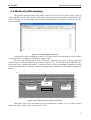
5.4.
Modes of profile mapping .................................................................................... 57
5.5.
Mapping scale ....................................................................................................... 58
5.6. Measuring tools .................................................................................................... 59
5.6.1. Epsilon measurement. Hyperbola .................................................................................. 59
5.6.2. Wave velocity measurement. Inclination. ...................................................................... 61
5.6.3. Velocity and epsilon measurement. Godograph ............................................................ 62
5.6.4. Depth and distance measurement .................................................................................. 63
5.7.
Additional profile snap-to .................................................................................... 64
5.8. Profile visualization .............................................................................................. 65
5.8.1. Change of profile color ................................................................................................. 65
5.8.2. Brightness and contrast control ..................................................................................... 66
5.8.3. Gain control.................................................................................................................. 67
5.9. Work with traces ................................................................................................... 70
5.9.1. The oscillogram of the trace. “Trace window” dialog.................................................... 70
5.9.2. Trace editing, profile cropping ...................................................................................... 72
5.9.3. Compacting. Profile adding .......................................................................................... 73
5.9.4. Selection of visible profile traces .................................................................................. 73
5.9.5. Labels on a profile. Photo labels. .................................................................................. 73
5.9.6. Adjusting the trace position .......................................................................................... 77
5.10. Change of a Profile relief ..................................................................................... 78
5.11. Splitting of a multichannel profile ....................................................................... 79
5.12. File export ............................................................................................................. 80
5.13. File import ............................................................................................................. 80
5.14. Data processing.................................................................................................... 82
5.14.1. Average substraction .................................................................................................... 82
5.14.2. Median filtering ............................................................................................................ 83
5.14.3. Horisontal median filter ................................................................................................ 84
5.14.4. Trend deleting .............................................................................................................. 84
5.14.5. Profile reversion. .......................................................................................................... 84
5.14.6. Invers correction ........................................................................................................... 86
5.14.7. Leveling ....................................................................................................................... 86
5.14.8. Aperture synthesis ........................................................................................................ 86
5.14.9. Hilbert transform .......................................................................................................... 87
5.14.10. Bandpass filtering. ........................................................................................................ 88
5.14.11. Horisontal filter ............................................................................................................ 91
5.14.12. Reverse filtering ........................................................................................................... 93
5.14.13. Smooth ......................................................................................................................... 94
5.14.14. Emphasis ...................................................................................................................... 95
5.14.15. Spectrum field. ............................................................................................................. 95
5.14.16. Deconvolution .............................................................................................................. 95
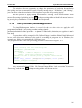
5.15. Use processing module application. .................................................................. 96
4
GeoScan32
Руководство пользователя
5.16. Processing history ............................................................................................... 97
5.17. Processing list creation ....................................................................................... 97
5.18. Print ....................................................................................................................... 99
5.18.1. Page setup .................................................................................................................... 99
5.18.2. Print preview ................................................................................................................ 99
5.18.3. Print............................................................................................................................ 100
5.19. Data saving ......................................................................................................... 101
5.19.1. Save image to a file .................................................................................................... 101
6. LAYER-BY-LAYER INTERPRETATION OF PROFILES ........................................... 102
6.1.
Peculiarities of by-layer interpretation mode ................................................... 102
6.2.
Creation of a profile with layers. ....................................................................... 103
6.3.
File peculiarities in mode of layer-by-layer interpretation .............................. 103
6.4. Drawing layers on a profile................................................................................ 104
6.4.1. Hand-drawing of layers .............................................................................................. 104
6.4.2. Semi-automatic drawing layers ................................................................................... 105
6.5.
Layer properties ................................................................................................. 106
6.6. Layer editing ....................................................................................................... 107
6.6.1. Layers selection .......................................................................................................... 107
6.6.2. Delete layers ............................................................................................................... 108
6.6.3. Layer editing .............................................................................................................. 108
6.6.4. Dragging a zero of a depth scale ................................................................................. 110
6.6.5. Trace window on the profile with the layers ................................................................ 110
6.7. Export of a stratified (.ldt) file ............................................................................ 111
6.7.1. Export to the Autocad (.dxf) format ............................................................................ 111
6.7.2. Export to .htm............................................................................................................. 113
6.7.3. Export of a text file "Amplitudes" ............................................................................... 114
7. 3D-VISUALIZATION MODULE OF GEOSCAN32 PROGRAM .................................. 115
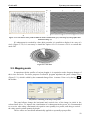
7.1.
Module description............................................................................................. 115
7.2.
Module opening. Files selection ....................................................................... 115
7.3.
Operation with an open file set. ........................................................................ 116
7.4.
3D – visualization mode ..................................................................................... 118
Appendix 1. License agreement. ................................................................................. 120
Appendix 2. Signal of electromagnetic interference description.............................. 122
Appendix 3. File date of GeoScan32 program, format F4 .......................................... 123
5
GeoScan32
Руководство пользователя
6
Руководство пользователя
GeoScan32
2. Preparation of program run
2.1. Program purpose
GeoScan32 Program is designated for control of the ground penetration radar (GPR), as well
as for further processing and visualization of the data obtained in process of scanning.
Program allows:
•
•
•
•
•
•
•
to record data from the GPR into a file
to print the radarogram;
to export files to other processing programs;
to process by layers;
to represent data in 3D format;
to apply color palette for design;
to process files and etc..
2.2. System requirements
Computer — Pentium CPU, running at 1000 megahertz or better.
RAM – minimum 256МByte. Recommend is 2GB.
Videocard –minimum 32 MB of video memory.
Free hard disk space – to store data 2 GB free space on a disk for each hour of operation is
recommended.
Ports – Ethernet port.
Operating system – Windows 2000, Windows XP, Windows 2003, Windows Vista.
7
Руководство пользователя
GeoScan32
2.3. Installation
The CD that came with the GPR package contains the documentation and program
GeoScan32 that you need install. A full disk description is given in the Appendix 4.
Program setup order:
1. Place the CD to the optical drive. The CD automatically displays the setup menu if Autorun is
enabled in your computer. If Autorun is NOT enabled in your computer, browse the contents of
the CD to locate the file “Logis.exe” from the BIN folder. Double-click the “Logis.exe” to run
the CD.
2. The menu shows the technical description for GPR and program GeoScan 32 for Windows XP
and Windows Vista.
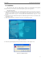
3. Click “Setup GeoScan32 for Windows Vista (XP”) for install the program;
Figure 2.3.1. Disk menu
4. Select the required language in the open window and press “OK” (Figure 2.3.2)
Figure 2.3.2. Language selection
8
Руководство пользователя
GeoScan32
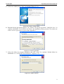
5. In the next window press “Next” to continue (Figure 2.3.3.)
Figure 2.3.3. Master setting window
6. Read the license agreement (Figure 2.3.4.), choose “I accept the agreement” and click “Next” to
continue installation. If you decline the license, the installation cannot proceed. The whole text
of the «Licence agreement» is given in the Appendix 1.
Figure 2.3.4. Licence agreement
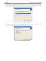
7. Select the folder for program installation and click “Next” for continue. Default folder for
installation is “C:\Program Files\GeoScan32” (Figure 2.3.5).
Figure 2.3.5. Folder selection
9
GeoScan32
Руководство пользователя
8. Select the program version: “SSE optimized GeoScan32” – special for Pentium 4, Pentium Core
2 Duo, Athlon 64, Sempron processors and allows to speed-up processing procedures setting
option or “GeoScan32 for generic processor” – special for low speed processors.
Figure 2.3.6. Program configuration selection
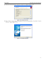
9. If you want to create desktop icon and start menu folder check the “Create a desktop icon” and
“Create Start Menu folder” options. (Figure 2.3.7) and press «Next».
Figure 2.3.7. Program configuration selection
10
Руководство пользователя
GeoScan32
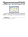
10. Check the selected parameters and press «Install » to continue (Figure 2.3.8).
Figure 2.3.8. Program setup data
11. Press “Finish” for exit Setup. The program will start up automatically, if you check “Launch
GeoScan” option (Figure 2.3.9).
Figure 2.3.9. Finishing installation
11
Руководство пользователя
GeoScan32
3. Beginning working with GeoScan32
3.1. The first start
Double-click the desktop icon “GeoScan32” (figure 3.1.1 (a)) or run program from Start
menu. (Figure 3.1.1(b)).
а)
b)
Figure 3.1.1. Start the GeoScan32 program
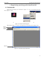
Main window (figure 3.1.2) allows selecting the type of operation you are going to start.
Header
Main menu
Toolbar
Status bar
Figure 3.1.2. GeoScan32 Program main window
12
Руководство пользователя
GeoScan32
The program window view changes partially according to the mode of operation being
executed. A window without open files contains the following:
•
Header - displays the program name or file name;
•
Main menu – gives access to every function and feature of program. GeoScan32 uses a
standard Windows Menu Bar. Menu selections that are ON/OFF toggles use a checkmark to
indicate their status.
•
Toolbar - provides buttons for the more frequently-used commands. The toolbar changes
depending on the mode in which the program operation is executed
•
Status bar - gives status information and properties of selected files and menu items.
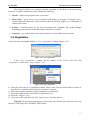
3.2. Registration
At the first start the program displays a “User registration” window (Figure 3.2.1).
Figure 3.2.1. User registration
If the “User registration” window did not display in the screen, select the item
“Registration” in the menu “Help” (Figure 3.2.2)..
Figure 3.2.2. User registration
1. Put in the user name in a registration window. Please, note! The user name shall be written as
specified in a registration form with due attention to a register;
2. Chose the program registration option (standard or professional);
3. Put in the registration key specified in a registration form.
4. Press the “Registry” key;
5. After successful registration the item “Registration” becomes inactive.
Warning! The unregistered program version works only with the files allocated in the root
directory of the Logis disk, in DEMO_FILES folder
13
Руководство пользователя
GeoScan32
•
•
•
•
•
•
•
The standard program version lacks the following modes and processing options:
3D view;
Bandpass, reverse, horizontal filters;
Spectrum field;
Aperture synthesis;
Smoothing;
Emphasis;
Average subtraction;
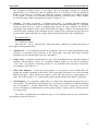
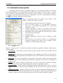
3.3. Program settings
3.3.1. Main window
“View” menu lets change main window view. Toolbar and status bar panels can be hidden
or displayed by choosing the “Toolbar” or “Status bar” items (Figure 3.3.).
Figure 3.3.1. Main window view settings
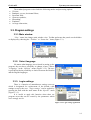
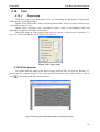
3.3.2. Select language
No matter what language was selected in setting up the
program, the user has a possibility to change it later. Choose
“Language” in the “Options” menu (Figure 3.3.2). The user
is provided with the possibility to choose between the Russian
and the English languages.
Figure 3.3.2. Language adjustment
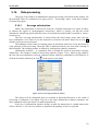
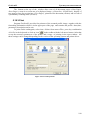
3.3.3. Logis settings
There is a function of manufacturer settings recovery
which is designated for replacement of the default value
settings set up by the user. “Logis settings” can be applied by
pressing the item with the same name in the “Special” menu
(Figure 3.3.3).
It is useful to apply this function when there are
program errors that can be caused by the parameters which
were wrongly set for.
Figure 3.3.3. Logis settings application
14
Руководство пользователя
GeoScan32
3.4. Document opening and creation
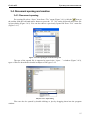
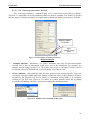
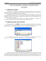
3.4.1. Document opening
For opening file select “Open” item from “File” menu (Figure 3.4.1) (click the
icon on
the toolbar with the left-hand mouse button or press the ”F3” key on the keyboard) and select file
in Open dialog (Figure 3.4.2). You can also choose a previously opened file from “File” menu list
(Figure 3.4.1).
Figure 3.4.1. File opening in GeoScan32 Program
The type of the opened file is supposed to open in the “Оpen…”» window (Figure 3.4.2),
types of files are described in details in chapter of file types 3.4.2.
Рисунок 3.4.2. Open dialog
Files can also be opened by double-clicking or just by dragging them into the program
window.
15
Руководство пользователя
GeoScan32
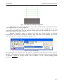
3.4.2. New document creation
The program allows to create different types of files such as “Profile”, “3D view” or
“Layers on the profile”. The program functional capabilities depend on the type of the open file.
The type of created file is selected in the “Create…” window (Figure 3.4.3). The window is
opening by one of the possible ways:
• Select the “New document” item in the “File” menu (Figure 3.4.1);
•
•
•
Left-click the
icon in the toolbar;
Press the “Ctrl+N” on the keyboard;
Figure 3.4.3. A new document creation window
Profile
Files with a profile are the result of saving the radarogram from scanning mode (full
description of a scanning mode is given in Chapter 4). All files have the extension GPR2 (GPR in
all versions lower than 2.5) marked with an icon shown in Figure 3.4.4.
Figure 3.4.4. The file icon with a profile
Layers on a profile
Files with layers appear after saving the changes in “Layers on a profile” mode (a full
description of the mode is given in Chapter 6), all of them having an extension LDT. A file with
layers always arises from GPR2 (GPR) file and is intimately connected with it, i.e. it is necessary to
move or copy both files, otherwise LDT will be unreadable. The icon identifying this file is shown
in Figure 3.4.5.
Figure 3.4.5. An icon of a file with layers
16
Руководство пользователя
GeoScan32
3D View
The GPR set of files is packed arranged in a 3D picture. This type of files has an extension
PRD are marked with an icon, shown in Figure 3.4.6. A full description of 3D visualization is given
in Chapter 7.
Figure 3.4.6.An icon of a 3D view file
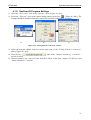
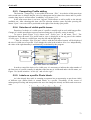
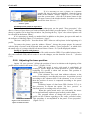
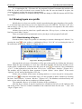
3.5. Copy files from the Processing Unit
GeoScan32 Program provides the possibility of contact with the processing unit for file
copying. In order to provide connection, it is necessary to connect it to the computer (the order of
connection is described in Operational Manual for «ОКО-2» GPR). Then select the “Processing
unit” item from the “Special” menu (Figure 3.5.1).
Figure 3.5.1. Activation “Transfer profiles from the Processing Unit” window
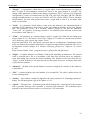
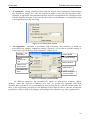
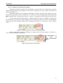
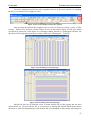
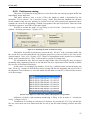
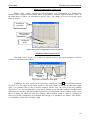
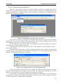
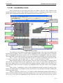
“Profile moving from Processing Unit” window (Figure 3.5.2) allows to execute file
copying from the Processing Unit and vice versa.
Processing unit total and
free memory
Computer total and free
memory
Destination folder
Create new folder on the
computer
Copy all files to the
computer
Copy selected files to
the computer
The list of
files from the
processing
unit
Copy selected files
from the computer to
the processing unit
Copy all files from
selected folder of the
computer to the
processing unit
Delete selected
file(s)
Refresh t
e PU’s list of files
Select destination
folder
Figure 3.5.2. Profile moving from Processing Unit
17
Руководство пользователя
GeoScan32
All files which are stored in CPU’s memory (including the palette files (*.CS)) are displayed
in the left-side of the window.
The folder tree, located on the right side of the “Profile moving from Processing Unit”
window, displays the folders of your file system as a tree. Select folder for copying files. Full adress
of the folder is displayed in the line “Destination folder”.
In order to create a new folder add its name to this line and press the key “Create folder”.
There are provided four keys for file copying the functional meaning of which is described
in Figure 3.5.2.
1. Before the beginning of copying mark one or several files for coping with the help of the mouse,
keys Ctrl or Shift in the keyboard;
2. Copy all files by pressing one of the copy keys. (Figure 2.3.32);
3. Wait for completion of copying and close the window by pressing the “ОК” button.
3.6. Reference system
Interface elements are accompanied with the pop-up help when the mouse cursor is pointed
to them (Figure 3.6.1).
Figure 3.6.1. Pop-up help
Keyboard shortcuts allow to speed data processing and recording operations.
Program instruction description displayed in the “GeoScan32 Reference” window which is
enabled by the item «Topics list» from the “Help” menu (Figure 3.6.2).
Figure 3.6.2. Reference widow in GeoScan32
Figure 3.6.3. Program data window
Compilation data and program version are displayed in the “About GeoScan32 Program”
window (Figure 3.6.3), entered by the item with the same name in the “Help” menu.
18
Руководство пользователя
GeoScan32
4. GPR scanning
4.1. Interface with GPR
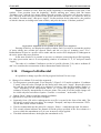
4.1.1. PC network settings.
GPR control is executed by GeoScan32 Program through the Ethernet connection effected
via RJ-45 connector or WiFi-adapter with the use of radio modem. The connection rate is from 0 to
100 МB/sec. In order to operate successfully, a correctly adjusted Ethernet adapter is required
4.1.1.1. Network adapter connection check.
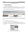
1. Open the “Network connections” window («Start» «Settings» «Network connections»);;
2. Test the applied connection state via the local network in the “Status” column (Figure 4.1.1);
Figure 4.1.1. «Network settings» window
If the local network connection state is in the “Disabled” mode, you should click the right
mouse button on the line “Local area connection” and select the “Enable” line in the displayed
menu;
3. Close the «Network connections» window
4.1.1.2. Network adapter connection rate adjustment.
1. Open the «Network connections» window («Start» «Settings» «Network settings»);
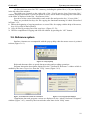
2. Click the right mouse button on the name of connection used for interface with GPR and choose
the “Properties” line. The selected Ethernet network adapter properties panel will display
(Figure 4.1.2);
Figure 4.1.2. The Ethernet network adapter properties panel
19
GeoScan32
Руководство пользователя
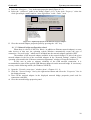
3. Press the “Configure…” key in the open properties panel (Figure 4.1.2);
4. Select the “Advanced” panel in the dialog (Figure 4.1.3). In the item “Property” select the
«Link Speed/duplex mode» and set “Auto negotiation” in the “Value” item.
Figure 4.1.3. Optional properties of the Ethernet network adapter.
5. Close the network adapter properties panel by pressing the “ОК” key.
4.1.1.3. Network bridge configuration check.
When there is a device i1394 (Fire Ware) ( in addition to Ethernet network adapter) or some
other devices of that sort, the operating system Windows automatically creates the type of
connection “Network bridge” which can be included into the network adapter applied in GPR.
The attribute of the network adapter available in the network bridge is a lack of the given
network adapter in the list of the accessible adapters in the “Network settings” window of the
operating system and in the “Ethernet-connection adjustment” window of Program GeoScan 32 .
In this case in order to enhance reliability of the GPR network connection, it is
recommended to turn off the applied GPR Ethernet-adapter from the network bridge. It is necessary
to carry out the following actions (for Windows XP RUS):
1. Open the “Network connections” window (item 1, Chapter 4.1.1.1);
2. Click the “Network bridge” line by the right mouse button and select the “Properties” line in
the displayed menu;
3. Turn off the network adapter in the displayed network bridge properties panel used for
connection with GPR;
4. Close the network bridge properties panel.
20
Руководство пользователя
GeoScan32
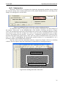
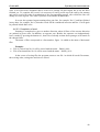
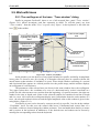
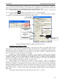
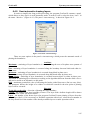
4.1.2. GeoScan32 Program Settings
1. Select the “Port select” item in the “Options” menu (Figure 4.1.4(а));
2. Select the “Ethernet” port in the opened dialog and press the key “ ” (Figure 4.1.4(b)). The
settings should be installed when the Control Unit is turned on and under operation;
а)
b)
c)
Figure 4.1.4.”Tuning Ethernet connection” window.
3. Select the network adapter from list in the upper part of the “Tuning Ethernet connection”
dialog (Figure 4.1.4(c));
4. Press the key «
» (the mode “Adapter autotuning” is inactive –
no tick off mark.
5. Network connect was a success if the first three values in the lines «Adapter IP address» and
“Radar IP address” coincide;
21
Руководство пользователя
GeoScan32
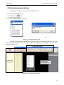
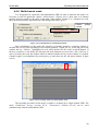
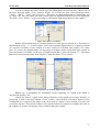
4.2. Scanning mode start-up
Scanning mode window can be started by different ways:
•
File >Scan (Figure 4.2.1(а));
•
•
•
Left-click on the
icon;
Ctrl+S in the keyboard;
File>New>Profile (figure 4.2.1(b)).
а)
b)
Figure 4.2.1. Scanning mode start-up
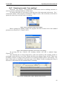
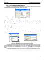
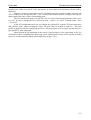
If all the above mentioned settings were adjusted in the right way and GPR ready to work,
the scan mode window with data from GPR (radarogram) will display over the main
window.(Figure 4.2.2)
Scanning parameters
Control
keys
Visualization
Current trace
oscillogram
Radarogram
Contextual
menu
Figure 4.2.2. Scanning mode window
22
Руководство пользователя
GeoScan32
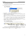
4.3. Scanning mode window
The scanning mode window can be conditionally divided into several parts which are
painted in different colors in Figure 4.2.2.
4.3.1. Control keys
Figure 4.3.1. shows all control keys.
Type of antenna unit
Figure 4.3.1. Control keys
•
•
•
•
•
Key “Connect ” – ON/OFF connection with GPR. Keyboard shortcut - “С”;
“Record” - start of profile recording. Keyboard shortcut - «R». A full description of profile
recording and saving is given in Chapter 4.4;
“Step” - use this button for recording each new trace in “Step-by-step” mode. In others modes
button allows to affix a mark. A detailed description of scanning modes is given in Chapter
4.3.4.2;
“Save” - 1) “Record” key is held - the “Save” key allows to save the recorded data which are
stored in the RAM of a computer from the moment of pressing “Record” button.
2) “Record” is released - “Save” key allows to save a file of a 2 screens size.
Keyboard shortcut - «S». A detailed description of a file saving order is in Chapter 4.5;
“Param” - opening “Scanning parameters” window. Keyboard shortcut - “P”. A detailed
description of scanning parameters is in Chapter 4.3.4;
4.3.2. Visualization setting
Use slider controls for changing brightness, contrast and gain level. (Figure 4.3.2).
Brightness
Contrast
Select
AGC/Gain
Gain
adjustment
Figure 4.3.2. Visualization setting panel
All sliders are designated to change parameters of radarogram drawing. If the slider moves
to the left, the parameter values decrease, and if it moves to the right, they increase. For returning to
default values left-click on “ ”button for intensity and “ ” button for contrast.
23
Руководство пользователя
GeoScan32
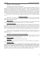
4.3.3. Current trace oscillogram
The oscillogram accepted at a current time of a trace (Figure 4.3.3) is displayed in the left
part of a scanning mode window. In this field display form of a signal, its maximum amplitude and
a vertical scale which can be expressed in nanoseconds (time of an electromagnetic wave in the
environment) (Figure 4.3.3 (a)) or centimeters (penetration depth of this wave) (Figure 4.3.3 (b)).
For switching a scale type from nanoseconds to centimeters, click it by the left mouse button.
Maximum
amplitude
Signal
form
Depth scale,
cm
Fill scale
Time scale
а)
b)
Figure 4.3.3. The oscillogram in a scanning mode window
4.3.4. Scanning parameters
4.3.4.1. The scanning mode window
Most often changeable scanning parameters are given in the field marked with orange color
in Figure 4.2.2, some of them are doubled in a window «Scanning parameters» (Section 4.3.4.2)
Рисунок 4.3.4. Параметры сканирования в окне сканирования
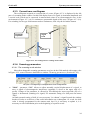
•
"Shift" - parameter “Shift” allows to adjust smoothly vertical displacement of a signal, to
move a signal of electromagnetic interference (appendix 3) closer to the upper edge of a
profile. Change of the parameter is effected by left-clicking the arrows upwards (rise of a
signal) or downwards (omitting of a signal). For automatic setting of a shift press the button
"Shift.
At hand-operated setting of shift it is not necessary "to exhaust" a signal beyond the window
borders in order to avoid loss of the useful information on a radarogram. As a rule, the shift
value is already programmed in the antenna unit, but if it is necessary to update it, it is
necessary to effect installation prior to the beginning of a profile record.
24
GeoScan32
Руководство пользователя
•
"Rough" – is a parameter, which allows to roughly adjust vertical displacement of a signal to
move a signal of electromagnetic interference closer to the upper margin of a profile. The
change of this parameter is similar to the change of parameter "Shift". One step of a rough shift
corresponds to 32 steps of a smooth one (for АB-1700, АB-1200, АB-1000, АB-700, АB-400
and their modifications) or to 4 steps (for АB-250, АB-150, АB-90, ABDL "Triton" and their
modifications). At work with greater time scales a rough shift is reset to 0, no matter what
value was set before.
•
"Scale" –is a parameter which defines a time scale and influences the maximum depth of
scanning. Scales changes by steps and its values can change depending on the used antenna
unit. The parameter "Scale" in a scanning window (Figure 4.3.4.) and the parameter
“Time scale” in a window “Scanning parameters” are identical. Scale selection is carried out
in accordance with Table 4.3.1.
•
"Gain" – the parameter in a window shows a gain of a signal. Use slider bar for change gain
factor (Figure 4.3.2). The button "AGC/Gain" (Figure 4.3.2) allows to switch between mode
АGC (automatic gain control) and a mode "Gain".
In the activated mode АGC (the button is pressed) there is an alignment of amplitudes so that
in the set window the maximum amplitude of a signal was approximately identical. The size of
an alignment window changes in a window «Scanning parameters» (Figure 4.3.5, section
4.3.4.2).
In the activated mode “Gain” program use user’s gain profile and gain factor.
•
“Begin” - a window indicates a coordinate of the profile beginning in millimeters. The entered
value is recorded into a file as a coordinate of the first trace and next traces are assigned a
value with taking into account the initial coordinate. The function works only when the key
“Begin” is held. If the key is not activated, the profile begins from zero, no matter what value
is specified in a window.
•
“Distance” - the data of the passed distance in meters is mapped in a window if the odometer
is operated on.
•
“File” - a window displays the serial number of a recorded file. The value is nulled at the exit
from a scanning mode
•
“Stacks” – this window completely duplicates the same parameter in “Scanning parameters”
dialog. The full description is given in Chapter 4.3.4.2.
•
“Speed” – The upper line – maximum speed and the bottom line - actual speed of the operator
with a georadar moving if the operation is executed with odometer. The maximum speed
depends on the interval between traces (see Section 4.3.4.2) and stacks.
25
Руководство пользователя
GeoScan32
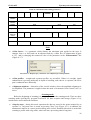
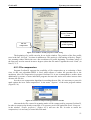
4.3.4.2. The “Scanning parameters” window
The “Scanning parameters” window (Figure 4.3.5) is entered by pressing the key “Param”
(Figure 4.3.1) and allows to set all parameters which are used in scanning. The window is divided
into the groups of similar parameters. For application of default parameters press the key "Default".
Apply parameters
“by default”
Open
optional settings
panel
Figure 4.3.5. The window “Scanning parameters”
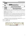
Basic parameters
•
«Samples Amount» - Maximum - 511 points. Parameter value may be decreased together
with the loss of part of information in the lower part of the radarogram. For example, if a
samples amount changes from 512 to 256 at time scale of 50 ns, the signal "will be cut off"
from below exactly by half and time scale will change from 50ns to 25ns.
•
«Traces amount» - this parameter limits the trace quantity in the recorded profile. Traces are
recorded in a program buffer until their quantity reaches the value of this parameter, all traces
accepted by the program will not be stored (a Continuous saving mode is an exception
(Section 4.5.2)). Fill scale (Figure 4.3.3) allows to visually quantity traces left to ending
record, the full shading with blue color means reaching the maximum rating.
Figure 4.3.6. Definition of the maximum profile length
26
GeoScan32
Руководство пользователя
The minimum parameter value is 100 traces, and its maximum depends on computer
characteristics or is limited by value of 640000 traces. It is possible to learn the maximum
length of a profile for a computer on which the program is installed in a window (Figure
4.3.6), which is entered by a command «System memory» from the menu "Help" (Figure
4.3.6) of the main window of program GeoScan32 (Figure 3.1.1).
•
«Stacks» - In order to increase “a signal-to-noise ratio”, a georadar performs hardware
accumulation of measurement results in each point with subsequent smoothing, i.e, a georadar
collects several traces in a point of scanning and records one trace, which is the result of
smoothing. This parameter value can be fixed within the range 1-100000. The minimum value
is defined, when scanning at the maximum speed is required. The parameter increase allows to
reveal weaker signals and improves image quality, but thus slows down the scanning rate.
Recommendations:
1-4 – Fast scanning
8-32 –Moderate tempo
more than 64 – use in “Step-by-step” mode and under conditions of strong absorption of
poor signal or strong interference.
•
“Epsilon*10” - in recording the profile the parameter value is set with approximation (this
parameter is calculated more precisely in the processing). The table with main electrical
parameters of the soil and solid is given in Appendix 5.
•
«Time scale» - Parameter which defines a time scale and influences the maximum depth of
scanning. The parameter "Scale" in a scanning window (Figure 4.3.4.) and the parameter
“Time scale” in a window “Scanning parameters” are identical. Scale selection is carried out
in accordance with Table 4.3.1.
•
«File series number» - It sets file series number, i.e. the names of all recorded files will
include the number identified in this field. Files in program GeoScan32 are saved in format
P0000_0000.gpr2, where the first four figures - series, and the next ones - order number, i.e.
if the “file series number” is 35, then the file will be stored with the name P0035_0000.gpr2.
•
«Scroll speed» - is a parameter which allows to control the radarogram movement rate in a
scan window. The maximum visual display rate is achieved at parameter 4, and the minimum
one is at parameter 1. At that with the rate value being 2, one trace is drawn per pixel of the
screen, accordingly, in enhancing the rate the picture image is spread, and in reducing the rate
it is compressed.
The values recommended for different types of the antenna units by the manufacture
specialists are given in Table 4.8.1.
27
Руководство пользователя
GeoScan32
Table 4.8.1. Recommended scanning psrameters
ABDL
АB90
АB150
АB250
АB400
(АB400Р)
Samples
amount
511
Traces
amount
>30000
Stacks
8-16
Time scale
АB1000R
АB1200
8-16
Epsilon
Interval
between
traces
Gain
АB700
АB1700
4-8
Appendix 5
-
150
50-100
30-50
-
10-30
10-40
200-400
200
50-100
24-48
16-32
Gain
•
«Gain factor» - is a parameter which denotes the maximum gain applied to the trace. It
changes from 1 to 9999 and can be adjusted both by a slider box of enhancement (Figure
4.3.2), and by changing the numerical value of the parameter in the “Enhancement” line
(Figure 4.3.7).
Рисунок 4.3.7. Параметры усиления в окне «Параметры сканирования»
•
«Gain profile» - straight and exponent profiles are accessible. When it is streight, signal
enhancement is growing uniformly in depth of unrolling, and when it is exponent, the lower
part is enhanced more drastically
•
«Alignment window» - dimension of the vertical window where the amplitude alignment is
accomplished. The parameter is applied when the mode of Automatic Gain Control (AGC) is
active;
Scanning mode
Before the beginning of scanning it is necessary to select the scanning mode. There are three
scanning modes provided by program GeoScan32 for data reception and storage (Figure 4.3.8),
which can be used in different situations.
•
«Step-by-step» - during this mode operation the data are stored in the points marked by an
operator, i.e. each new trace is stored on pressing ”Step” key (Figure 4.3.1); in addition, the
antenna unit shall be in a static position during trace record. Normally this mode is used while
scanning a profile with a big stacks, when each trace processing takes a long time.
28
Руководство пользователя
GeoScan32
•
«Continuous» - During operation in this mode the data are stored continuosly. Data memory
rate depends on Stacks. As a rule, the continuous mode is used when the operation with a
odometer is impossible, but sometimes the data record is accomplished in a continuous mode
with the attached odometer, in this case the data of the covered distance is stored and its setup
is accomplished in profile processing
Figure 4.3.8. Scanning mode selection
•
«On migration» - operation is performed with a odometer, the parameters of which are
prescribed in the window “Odometers settings” (Figure 4.3.9). In order to open the window, it
is necessary to press the key “Select odometer” (Figure 4.3.8).
Odometer with
wheel DP-32
Wireless DP32R
Automobile odometer
Built-in
odometer АB1700
Railway odometer
Odometer with
spool of thread
Wheel diameter
Search Bluetooth
devices
Amount of impulses
on a turn of wheel
Figure 4.3.9. Odometer selection window
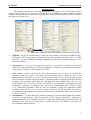
Six different odometers, the parameters of which are indicated in windows “Wheel
diameter” (mm) and “Amount of impulses on a turn” are provided for operation with GPR.
Normally these parameters are set automatically after pressing the key with the suitable name, but
there is also a possibility provided for self-updating of these data in order to take into account the
peculiarities of the location or the changes in the design of the odometer (e.g. wheel replacement)
29
Руководство пользователя
GeoScan32
DP-АB1700
During operation with antenna units АB-1700 and АB-1200 with the built-in odometer it is
necessary to press the key «DP-АB1700», whereupon the odometer parameters will appear in the
above mentioned windows: diameter – 5 mm, amount of impulses – 32.
DP-32
At usage of odometer DP-32 with a standard wheel it is necessary to press the button “DP32”, then the parameters will change: diameter – 22 mm, amount of impulses –32.
Spool (GP)
In case of work with a odometer Spool(GP) (odometer with a spool of thread), press the
button “Spool (GP)”. Odometer parameters: diameter – 16, amount of impulses – 10.
•
•
•
“Interval between traces” - Data in mode “On migration” are stored in equally-spaced
position points in the specified distance. The distance between two points is specified in the
line «Interval between traces» (Figure 4.3.8). The recommended step values for different
antenna types are given in Table 4.3.1.
“Calibrate” - In case of work with a odometer it is feasible to perform calibration before
scanning (See Section 4.3.5 in details)
“Reverse odd files” - can be used in carrying out areal survey for the subsequent threedimensional visualization when it is important to arrange scanning points in the nodes of a
regular rectangular mesh. It is for areal scanning that yet another option called “revers odd
files“ (Figure 4.3.9) is stipulated. Placement of a tick assumes pitch reversing of even files.
Usage of this function is justified during record of parallel profiles as an Indian file when the
end of the previous profile is in range with the beginning of the subsequent one.
Scanning mode selection can be performed immediately in a scanning window
For this purpose it is necessary to press the button which is outlined by a red oval (keyboard
shortcut is “V”) in Figure 4.3.10. This button accepts three values:
1. Migr – “On migration” mode;
2. Cont. – “Continuous” mode;
3. Step – “Step-by-step” mode.
Figure 4.8.10. Scanning mode change key
30
Руководство пользователя
GeoScan32
Optional panel
The optional panel opens by pressing the button «->> » (Figure 4.3.11). Some options which
are used not so often as the rest ones are included in it, in addition, this panel adjusts operation
settings with optional devices such a bar-code and GPS. Work with these devices will be considered
in Chapters 4.4.5 and 4.4.6.
Figure 4.3.11. Opening the optional panel
•
«Dipoles» - the given section allows to select the used dipoles in antenna unit ABDL"Triton".
The button “100” means usage of vibrators by frequency 100 MHz, the button «50» - 50 MHz
and «25» - 25 MHz. With the parameter changing, the filtering parameters and those of the
aerial base change.
•
«Attenuator» - in case of strong signals reception it is possible to use decay of a forward
signal by 20 dB which allows to avoid input amplifier overload. For activation of this mode it
is necessary to switch over the parameter to 20 dB.
•
«Dev. stack» - a device stack, means, that if the parameter value “Stacks” is less than the
parameter value “Dev. stack “ then stack will be performed only at a hardware level, in the
antenna unit, but if stack is set at the value that is more than a device stack, then the antenna
unit will transfer the data with stack equal to a hardware limit to program GeoScan32 and the
program will accumulate these data till obtaining total stack appointed by the user. By
increasing the value of a device stack it is possible to cut down time consumption for data
transfer into a computer, by making it more rarely. The recommended value of a device stack
is 16. When high parameter values are used in conditions of high level absorption media
scanning, there can be a loss of weak signals, generated by the algorithm of hardware
accumulation in the antenna unit. In this case a decrease in a hardware limit up to 8, and even
4 can prove useful.
«Decimation» - it is used when long profiles scanning is performed by high-speed georadars.
Activation of this function leads to reduction of the mapped information, reduction of
computational cost of a computer in order to reduce the accepted data processing time. In
particular, only each forty seventh trace is drawn. However, the memory unit stores all
accepted data without dropouts.
•
31
Руководство пользователя
GeoScan32
4.3.5. Contextual menu
In addition to the control keys to call some functions in a scanning window, provision is
made for the contextual menu (Figures 4.2.2, 4.3.12) which is activated by a right-click of in the
field of radarogram
•
«Connection» - an item backing-up the key of the same name in a
scanning window. It allows to make/break connection with GPR.
• «Record» - executes the same function as the key «Record» in the
scanning window, i.е. the beginning of profile.
• «Label» - sets a single lable on a profile. See the detailed
information about lable setting in Chapter 4.4.1
• «Parameters» - opens the window «Scanning parameters». It
duplicates the key “Param” in a scanning window.
• «Save» - See Chapter 4.5 for detailed information about saving;
• «Sets» - program GeoScan32 provides an opportunity of usage of
standard parameter sets. For instance, if the operation is often
executed in similar conditions. In selecting the given menu item, the
window (Figure 4.3.13) for selection of one of the standard sets
opens. The description of all standard sets is given in Appendix 7;
• «Record set» - the function allows to edit the available sets and to
Figure 4.3.12.
create its own ones. For this purpose it is enough to set the desired
Contextual menu
parameters in window “Scanning parameters” and select the item
“Record a set” in the contextual menu. Thereafter the edit window opens. (Figure 4.3.14).
Figure 4.3.13. Parameter selection set window
•
•
•
Figure 4.3.14. Edit window of the parameter
Button «New» - allows to memorize a new set after the title input;
Button «Delete» - deletes a chosen set from the list;
button «Change» - allows to edit the name and assigns the parameters prescribed in the
window «Scanning parameters». to the available sets
32
GeoScan32
Руководство пользователя
•
«Calibrate» - calibration of a odometer. In some cases, due to circumstances or features of a
surface, the odometer supposes a tangible systematic error of measurements. For example, in
case of movement on a smooth, slippery surface or loose sand, indications of the wheel sensor
are underestimated, and in case of movement on stony soil they can exceed actual
displacement. For calibration of the sensor before the beginning of a profile record, open the
panel «Odometer calibration» (Figure 4.3.15), by choosing the item of the contextual menu or
by pressing a combination of keys «Ctrl+T»
•
Measure a test distance (some tens of meters are recommended) on a roulette and put distance
length in millimeters into a window “Etalon distance “, then install the antenna unit so that the
wheel of the odometer was on a zero datum of a distance. Press the key "Start " and move the
antenna unit with the odometer along a reference distance (thus it is not necessary to write
down a file). After the wheel of the odometers on a final mark of a distance, repeatedly press
the key "Start", then the "OK". The odometer will be calibrated.
•
«Sounds» - Switching – on/off of the accompanying sound in program GeoScan32.
Sometimes it is useful to switch on a sound volume, since the basic actions of the program (the
beginning of record, origin of an error, the dropout of a line, etc.) are accompanied by
characteristic sounds.
•
«Pause» - Switching –on/off of the accompanying sound in program GeoScan32. Sometimes
it is useful to switch on a sound volume, since the basic actions of the program (the beginning
of record, origin of an error, the dropout of a line, etc.) are accompanied by characteristic
sounds.(keyboard shortcuts - Z or Pause );
•
«GPS» - activation of a panel working with GPS. A detailed information about work with
GPS is described in Chapter 4.4.5;
•
“Bore hole” - activation of the panel to control a bore hole GPR. Work description in a
window is delivered together with the device itself;
•
«Event log» - a window where the auxiliary information during scanning is mapped. It is used
in mode of “Continuous saving” and during operation with the barcode scanner.
•
«VideoScreen» - activation of the control panel by means of data from a videocamera and by
placing photo lables on a profile. The detailed description of operation with a video camera is
given in section 4.4.2
•
«Exit» - transfer from a mode of scanning into the main window of the program, also it is
possible to use keys X and Esc on the keyboard.
33
Руководство пользователя
GeoScan32
4.4. Record of Georadar Profile
Before the beginning of a profile record, be sure, that all parameters have been set and the
selected mode of scanning complies with working conditions. Settings adjustment and mode
selection is performed in accordance with Table 4.3.1 and recommendations of Chapter 4.3.4.
Without starting the profile record, check the operation of the odometer, i.e. the distance in a
corresponding window increases when the antenna unit is being moved, be also sure that the right
time scale has been chosen (Table 4.3.1) and shift has been set so that the signal of electromagnetic
interference is located close to the upper edge of the profile but at the same time it does not go
beyond the window borders.
Stack should also be chosen, following the recommendations stated above, and in setting
this parameter attention should be paid to the change of the authorized scanning speed which may
appear to be inadmissibly small when the stack is big that will strongly complicate work.
In the process of scanning it is worth paying attention to parameter “Scroll speed “ which
should be reduced during inspection of long sites since in this case a window includes more traces
which will allow to evaluate a radarogram in real time or to increase, in the course of short profiles
inspection
In order to start scanning, put the antenna unit on an index point of a profile and press the
key “Record” or the key R for the beginning of a record. Then as a result, the scanning window will
acquire the view as shown in Figure 4.4.1, i.e. the key “Record’ and “Param” becomes inactive.
Near the oscillogram of a current trace appears a fill scale, instead of a window "Roughly" appears
a window "Trace" in which the quantity of the accepted traces is calculated.
Trace counter
Fill scale
Figure 4.4.1. A scanning window during a profile record
Control the fill scale in the process of profile record in order to avoid loss of data. When the
scale is filled, i.e. the set value in the parameter “Traces amount” is achieved, profile record will
stop.
In accordance with the selected scanning mode start moving the antenna unit over the
surveyed area, each mode has its specific features of motion.
So in a mode "Continuous" try to slide with identical velocity without jerks so that there
were no sites of compression and expansion on a profile. It is possible to inhibit rate of profile
filling by means of increasing the stack value. If a profile record is accomplished in this mode with
the on-line odometer, despite of irregularity of movement, traces are placed in correspondence with
their true position on a profile (for this purpose it is necessary to include a mode “By trace
position” which is described in the section 5.9.6).
34
Руководство пользователя
GeoScan32
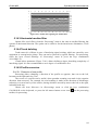
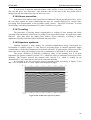
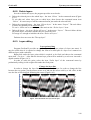
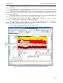
While scanning in mode “On migration” pay special attention to the displacement velocity
and be sure that it won’t exceed the permitted one. The permitted velocity depends on the stack
parameter. A radarogram is painted in black color in those places where the permitted velocity is
exceed (Figure 4.4.2), i.e. a vertical black line is drawn of the instead of a missing trace, besides a
sound signal is heard.
Figure 4.4.2. A radaragram part when the trace is missing
On retention of a file the missing traces are nowise denoted, that is why in order to receive the
materials suitable for processing, try to move without exceeding the permitted velocity. In order to
rewrite the missing traces, it is necessary to come a little back to the zone where the traces passed
right, meanwhile a radarogram will also move a little back, and on resuming the onward motion to
complete the profile without blanks.
When the operation is executed in mode “Step-by-step” тthe traces are recorded by pressing
the key “Step” in a scanning window or by pressing the keyboard shortcuts “Space” or “Insert” as
was described below, in this case when recording a trace it is desirable to fasten the antenna unit
motionless.
4.4.1. Labeling in profile scanning
4.4.1.1. Ordinal labels
Program GeoScan32 provides a possibility of labeling during profile record. For creation of
new labels in modes of scanning such as “On migration” and “Continuous” the key “Step” is used
in a scan window, the key “Space”, “M” or “Insert” are in the keyboard. For labeling in mode
“Step-by-step” only the key “М” is used in the keyboard.
Radarogram labels look like vertical red lines (Figure 4.4.3). Normally labeling is needed to
underline some abnormality. Labels are usually numbered sequentially ascending from the first.
35
Руководство пользователя
GeoScan32
Labels
Метки
Figure 4.4.3. Label representation in a scan window
4.4.1.2. Labels with names
If it is required to assign label names in the process of scanning, the program provides such
a possibility. For this purpose the text editor (for e.g. «Notepad») is created with extension «txt», in
which digits and label names are indicated in tabulated form:
1 pipe
2 cable
3 house
4 pit
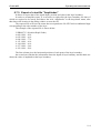
The figures in this table can change from 0 to 9 since numerical keys 0 through 9 are used in
scanning mode.
After creating a text file with a table during a scanning mode, double-click the radarogram.
Press the key «Open» in the opened window “Labels set” (Figure 4.4.4) and select the previously
created file. The content of this file will display in the window «Label set». After pressing the key
«OK» the given set is applied.
In order to set such a label within the scanning time, as it was already said before, it is
necessary to press any numerical key in the computer keyboarder after which the preset label will
be assigned a proper value. The name «1 pipe» will be assigned to the label after pressing “1”, on
pressing «2» there will be «2 cable» and so on. Different labels are painted in different colors, but
color and name labels are displayed only in processing mode.
Figure 4.4.4.Window «Labels set»
Labels are displayed in a scanning window as usual – as red vertical lines. In addition to
labels from the set the original ones can be put in the process of recording
36
Руководство пользователя
GeoScan32
4.4.1.3. Labels in «Continuous saving»
Program GeoScan32 stipulates the possibility to store profile series following each other
without interruptions. For this purpose is the mode «Continuous saving», which is described in
details in Chapter 4.5.2.
This mode assumes the continuous numbering of labels when the label number does not
depend on the quantity of the recorded files, i.e. when a new file recording starts, label numbering
does not begin from 1 but from the value n+1 where n is a number of the last label of the previous
file.
For activation of label numbering in a scanning window in mode of scanning, it is necessary
to include first «Continuous saving» (Chapter 4.5.2), second, press the key «Label», which displays
in the top part of the scanning window after switching on the mode of “Continuous saving” (Figure
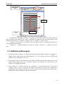
4.4.5).
Figure 4.4.5. Position of the key «Label » in a scanning window
After pressing this key there will display a window where an order number of a label in a
series of the recorded file is displayed.
Open “Video”
panel
Figure 4.4.6. Label meter under the key
37
Руководство пользователя
GeoScan32
4.4.2. Enter photo labels and “Video” panel
In addition to the common labels, program GeoScan32 provides an opportunity to enter
photo labels which are different from the original labels in the fact that they are accompanied by a
photo.
First, it is necessary to connect video camera to the USB computer port and to install a
proper driver. The connection order of a camera to PC and driver installation are usually described
in the documentation for a video camera. Upon connection it is necessary to start up a scanning
mode and to open the panel “Video” (Figure 4.4.7), by pressing the key of the same name in a
scanning window (Figure 4.4.6).
Obtained display
Change of
photos
parameters
Key of saving photos
into a file
Indicator of availability
of connection with a
camera
Camera selection panel
Autolabels parameters
Create new
photo label
Figure 4.4.7. “Video” panel
It is the video panel that allows to accomplish photo labeling. After its opening the
connection with a camera is installed automatically that is conformed by a tick against the caption
“Connect” Selection of the used video camera (if more than one camera is attached to PC) is
performed in a drop-down list in Figure 4.4.7 – the camera selection panel. The key “Ph-mark” or
the Key “A” in the keyboard is used for photo labeling. The key «Size» allows to call the window
позволяет вызвать окно «Image size selection» (Figure 4.4.8), in which the size of the saved
images and their quality is set. The key «File» allows to save the graphic file with a current image
apart from a radarogram.
Figure 4.4.8. Frame settings
In addition to a single label setting there is a mode of “Autolabel” in which photo labels are
set automatically with an interval equal to a step which is set by the user.The mode will be switched
on if you put in a tick mark against the word “Autolabels” (Figure 4.4.7), a step is set in the
window “Step(m)”. The proper functioning of this mode is provided only when a odometer is under
operation.
38
Руководство пользователя
GeoScan32
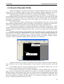
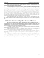
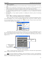
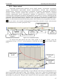
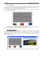
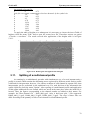
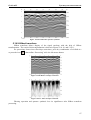
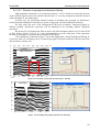
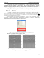
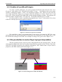
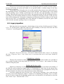
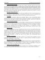
4.4.3. Substraction
The mode «Subtraction» is designated for displaying dynamically modified objects behind
the obstacles during static scanning and search of alive people behind the barriers according to the
change of a radarogram in a static mode.
Subtraction
Figure 4.4.9. Initialization of the “Subtraction” mode in scanning parameters.
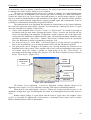
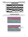
To enable this mode it is necessary to put a tick mark by clicking the left mouse button on
the caption “Subtraction” in the additional part of the window «Scanning parameters» (Figure
4.4.9). On activating this mode the profile displays the result of the coordinated subtraction of the
next received trace from the average trace array of the previously accumulated traces. (Figure
4.4.10). The quantity of traces used for “average trace” calculation is defined by a numerical value
located to the right of the option (Figure 4.4.9). The size of the accumulated traces array can be set
from 2 to 2000. In highlighting the dynamically modified objects it is recommended to set a
parameter equal to 50-60 and the stack equal to 8.
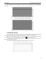
You can switch on/off the subtraction mode by a proper key (Figure 4.4.10) in a scanning
window. This key appears only after initialization of subtraction in scanning parameters.
Absence of movement
Movement at distance 2m from АБ
Figure 4.4.10. Scanning in the mode “Subtraction”
39
Руководство пользователя
GeoScan32
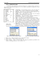
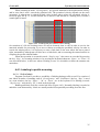
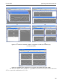
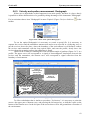
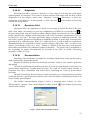
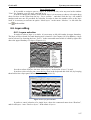
4.4.4. Multichannel mode
It is designated for operation with multichannel GPR. In order to initialize the mode it is
necessary to tick off against the caption “Multichannel” (Figure 4.4.11), there after a of channel
quantity selection window will appear to the right of the caption. Usually 2 or 3 channels are used,
but a maximum quantity depends on the GPR design and can be up to 8
Channel
selection
quantity
Figure 4.4.11. Initialization of a multichannel mode.
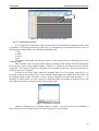
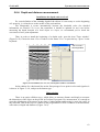
After initialization of the mode and selection of channel quantity a scanning window is
devided into several parts depending on the channel quantity. (Figure 4.4.12). In the top part of the
window the key “Number” (highlighted in red), which denotes the № of the recorded channel. If
the key is inactive (is not held), the data from all used channels are saved into a file, if the key is
active (is held), then only the channel which is indicated under the key in the window is recorded.
Channel toggle is accomplished by pressing key up and down by the left mouse button. (Figure
4.4.12).
Figure 4.4.12. Scanning window in multichannel mode.
The operating procedure in this mode is similar to scanning by a single-channel GPR. The
mode «Continuous saving» (section 4.5.2), "Decimation" (section 4.3.4.2) can be used
simultaneously with the multichannel GPR.
40
Руководство пользователя
GeoScan32
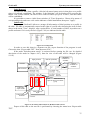
4.4.5. GPS operation
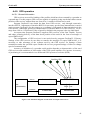
4.4.5.1. General information
GPS receivers are used for binding of the profiles which have been scanned by a georadar to
a ground map. For this purpose GPS receivers capable of regularly giving out the data about current
position of the receiver with uniform rate from 20 to 1 readout in second can be used.
Program GeoScan32 can obtain the data from GPS receiver only through consecutive
interface RS232. Adjustment of interface RS232 for necessary speed of data transmission is carried
out in program GeoScan32 for the purpose to co-ordinate it with speed of data transmission in the
GPS receiver. Admissible speeds of communication of interface RS232 for GPS receivers lie in a
range from 1200 to 115200 baud. Value of speed by default in the program is the size 9600 baud.
At current time Program GeoScan32 supports GPS receivers of the firm Trimble, Topeon
and others, allowing delivery of the data about position of the aerial in the form of messages of
report NMEA-0183.
The configuration of GPS receivers is not carried out by program GeoScan32. If factory
Settings of the GPS receiver do not allow to transfer the messages of report NMEA-0183, it is
necessary to take advantage of the software used by the GPS receiver for Settings of data
transmission under the specified report. Besides the receiver program Settings of allows to change
speed of communication.
Accuracy of definition of a georadar aerial position depends on characteristics of the used
GPS receivers and conditions of observation of the GPS system satellites. For increase in accuracy
of positioning it is recommended to use differential GPS systems of real time (RTK).
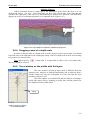
Satellites GPS
RS232
Receiver GPS
PC
(GeoScan32)
Antenna GPS
Mech. cont
Ethernet
Control unit
Antenna unit
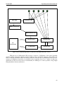
Figure 4.4.13 The Block diagram of connection of a simple GPS receiver
41
Руководство пользователя
GeoScan32
Satellites GPS
Base GPS
Antenna GPS
Radio modem GPS
Radio modem GPS
RS232
Receiver
GPS
Приёмник
Antenna GPS
GPS
PC
(GeoScan32)
Mech. cont
Ethernet
Control unit
Antenna unit
Figure 4.4.14. The Block diagramme of connection of the differential GPS receiver.
With the use of differential GPS receivers, accuracy of definition of the aerial georadar
position rigidly connected with the aerial of GPS receiver, essentially improves and reaches the
value of several centimeters under favorable conditions. With the use of elementary GPS receivers,
accuracy of definition of position is essentially worse, frequently from 5 to 15 meters. In that case
application of GPS receivers can be recommended, for binding to a card of profiles of big length
long (hundreds of meters and more).
42
Руководство пользователя
GeoScan32
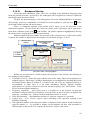
4.4.5.2. Switch on and work order
To start work with GPS it is necessary to connect it to port RS232. Then start program
GeoScan32. The control over the information accepted from the connected GPS receiver is carried
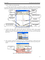
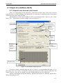
out by means of the panel «GPS info» (Figure 4.4.15) which can be activated by several ways.
Quantity of
satellites
Connection
speed
Time
Port
current
position
Height of antenna GPS
Choose scale
The route of
movement
Save rout in file
Move current position of
the aerial to the centre
Close “GPS info”
dialog
Figure 4.4.15. Description of “GPS info” panel
1. A choice of the item «GPS» from the menu "Special" in the basic window of the program
(Figure 4.4.16). Thus there is only a panel «GPS info» on the screen . It is usually used for
preliminary Settings communication and testing of the GPS receiver before the start of georadar
data record.
Figure 4.4.16. Start of “GPS info” panel
2. Open “GPS info” dialog from scanning mode. Open “Scanning parameters” window and to tick
off against the caption “On” in GPS group (Figure 4.4.17) and close window by pressing “OK”
button.
Start “GPS info”
panel
6
Choose connection
port
Connection
speed
Figure 4.4.17. Adjustment of GPS in scanning parametres
43
Руководство пользователя
GeoScan32
3. It is Also possible to open the panel by pressing a key «G» in the keyboard or by choosing an
item «GPS» from the contextual menu which can be opened by right-clicking in a window of
scanning.
Adjustment of speed and port choice is carried out both in parametres of scanning , and in a
window «GPS info». With the open panel «GPS info», program GeoScan32 guards port RS232
chosen by the user (its number can be different). In case there are enough GPS satellites (the
satellite quantity is shown in line «Sat»), the program displays the data about real time in line
"Time", about current position of the aerial in lines "Breath", "Longitude", "Height".
The route of movement of the GPS receiver aerial is shown with the dark blue line in a
window «GPS info», in the same place the co-ordinate grid which scale can change is drawn
(Figure 4.4.16). A key «Ц» is used to move current position of the aerial to the centre of a coordinate grid.
GPS data saving is possible only in recording georadar profiles . About the fact that the data
is saved, the tick against a word "Save" informs. Program GeoScan32 keeps the information
received from receiver GPS, in a separate file with expansion «.log». The file name coincides with a
name of a corresponding profile. Records in this file are made in a text format and contain both the
information on the changing position of the aerial, and time labels
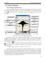
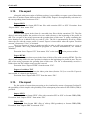
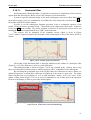
4.4.6. Work with a bar-code
4.4.6.1. General information
In program GeoScan32 the mode of an automatic recording of profiles on a signal from the
bar-code scanner is provided.
For work the antenna block (АB-1700 or АB-1200) and the device of bar-codes reading
which is connected to USB port of the notebook computer is used and fastened to the antenna unit
(the external view and the device itself are described in the Operational Manual on the Georadar
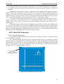
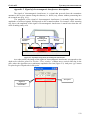
«ОКО-2»). Bar-codes are put on a marking mat (Figure 4.4.18) along a vertical and a horizontal
through each 5 cm. The used coding is Code 39.
Bar - code
Figure 4.4.18. A marking mat with bar - codes
44
Руководство пользователя
GeoScan32
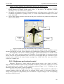
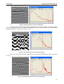
•
•
•
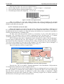
Each barcode (Figure 4.4.19) has its digital notation.
The first digit denotes a line direction: figure 1 – a vertical, figure 2 – a horizontal.
The second one denotes passage number from 1 to 21.
The third figure denotes the beginning – 0 or the end – 1 of a passage.
Digital notation
Figure 4.4.19. Bar-codes digital notation
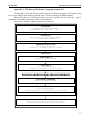
Thus, on reading of a bar-code which designates the passage beginning, the program
automatically begins profile record, and on reading of a bar-code of passage designating the end it
finishes record and saves a profile
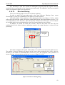
4.4.6.2. Activation and work order
Before the beginning of work connect the device of bar-code recognition to USB port of a
PC with which the further work will be carried out. Then install the driver from a disk which is
included into the device complete set. When all actions set forth above are executed, it is possible to
start the program and enter a scanning mode.
To start work with the bar-code scanner it is necessary to put a tick mark against an
inscription "On" (drawing 4.4.20) in section «Additional devices, the Bar-code" of a window
«Scanning parameters» and to choose a port of communication and speed of connection.
№ of COM port after driver’s installation can be checked in a window “Device Manager”.
For this purpose right-click the icon “My computer”» on a desktop, choose the item "Property",
then choose the entry "Equipment" in the drop-down window and press the key “Device Manager”.
You will see the numbers of ports used in the computer The open window “Device Manager” if
you unroll a menu branch «Ports (COM and LPT)» by pressing «+».
Speed of connection will be set equal 38400.
Choose
connection port
Start work with
bar-code
Connection
speed
Choose order of
scanning
Figure 4.4.20. Settings adjustment of a bar-code scanner operation
Press the key" ОК "in a window “Scanning parameters” after installation of all parameters
of communication with the bar-code recognition device.
Be sure that the device works, for this purpose when in scanning mode try to read one of the
bar-codes printed on a marked mat. If after reading is executed, the label is set in the radarogram,
then the device operates properly. In addition to a label, after reading is completed, a digital
designation of a bar-code can be found in a window "Event log" (Figure 4.4.21) which is caused by
the item choice «Event log» from the contextual menu.
45
Руководство пользователя
GeoScan32
Figure 4.4.21. Bar-code data report panel
Before the beginning of carrying out of the areal scanning arrange a marked mat on an
investigated surface. Try to fix it motionlessly avoiding sharp breaks in the locations of bar-codes.
The program allows to make scanning in various directions (a horizontal or a vertical) and in
various sequence. For this purpose 2 keys (Figure 4.4.20) are located in a window «Scanning
parameters», regarding bar-code options.
These keys form the following combinations:
1.
– At first there is a scanning along a vertical, then the program passes to
scanning across, along a horizontal.
– At first scanning across is carried out, then the program passes to scanning in a
2.
vertical.
3.
– Scanning is carried out only on a horizontal, then the program finishes
scanning.
4.
– Scanning is carried out only on a vertical then the program finishes scanning.
The top key shows in what direction scanning will initially be carried out, and the bottom
key shows whether scanning will be continued or not, and in what direction. In order to change the
value of the key, it is enough to click it with left mouse button.
46
Руководство пользователя
GeoScan32
At correct adjustment of the bar-code recognition device in the basic window of scanning,
the Key «#» becomes active (Figure 4.4.22).
Figure 4.4.22. Areal scanning activation key position
After pressing this button the program offers to select a folder for saving a series of files
(saving – Section 4.5), and then vertical (Figure 4.4.23) or horizontal (Figure 4.4.24) lines which
correspond to passes on a mat appear in a scanning window instead of a radarogram. Besides, the
direction of lines depends on the chosen values of the keys "Horizontals", "Vertical".
Figure 4.4.23.Scanning of vertical passages
Figure 4.4.23. Scanning of horizontal passages
Initially all lines are in dark blue color, it means that the file of this passage has not been
written down yet. To write down a file, it is necessary, by moving the antenna block in the chosen
direction, to read off a beginning bar-code then the line corresponding to the passage will change its
47
GeoScan32
Руководство пользователя
color in red. Red color designates that a record of a passage file has begun, but it has not been
finished yet. To complete the record, it is necessary to scan a profile up to the end by the antenna
unit and to read a bar-code of termination of the corresponding passage, after which the line will
change its color in green. The order of profiles record makes no difference.
In a case the operator began scanning along one line, for example, No.15, and has finished
in any other, for example, No.16, then the record will be considered incorrect and line 15 will again
be painted in dark blue color.
4.4.6.3. Completion of work
Scanning is completed or goes to another direction, when all lines of the current direction
are painted in green color. In addition, an operator can. Besides the operator can independently
leave a mode by pressing the button «#», thus files of already written down passages will remain in
the chosen folder.
The name of files corresponds to a line number, figure 1 is added to the name of horizontal
files.
•
•
Example:
File of vertical line No.19 will be stored with the name – Р0000_0019.
File of horizontal line No.19 will be stored with the name – Р0000_0119.
In the course of saving files the program creates a text file in which all saved files names,
their saving order, saving time and size are stored.
48
Руководство пользователя
GeoScan32
4.4.7. Scanning in mode “Iron seeking”
The mode “Iron seeking” is designated for reinforcement search in building structures, is
used on operation with high frequency antenna units
To activate this mode it is necessary to select the item of the same name in the menu “View”
of the main window of the program «GeoScan32» (Figure 4.4.24). After activation (a tick mark is
against the menu item) start up a mode of scanning.
Figure 4.4.24. Activation of mode «Iron seeking»
Before opening the scanning window the program will offer to choose one of the standard
parameter sets (Section 4.3.5, Figure 4.4.25).
Figure 4.4.25. Selection of parameter sets in mode “Iron seeking”
On pressing the key «Cancel», the scanning window will take a standard shape.
(Figure 4.2.2).
After choosing the set and pressing the key «ОК», the transition to the scanning window is
performed, in this case the view of the window itself does not change (Figure 4.4.26). There is no
possibility of choice or change of the parameters in a scanning window in mode “Iron seeking”. The
name of the used set is displayed in the upper part of the window. Profile recording and saving in
this mode is fully identical to the standard mode of scanning.
Figure 4.4.26. Scanning mode window “Reinforcement search »
49
Руководство пользователя
GeoScan32
4.5. Profiles saving
The main tool for saving profiles is the key “Save” in the main window of a scanning mode.
(Figure 4.5.1). An alternative to this key is the keys “S” and “Enter”.
Figure 4.5.1. Profile saving key
If a profile record is not logged (the key “Record.” is not held), then on pressing the key
“Save” a file of 2 screens size is saved.
If a profile record is being logged (the key “Record.” is held), then on pressing the key
“Save” the file the length of which is no more than the parameter “Traces amount” is saved.
In any case the key pressing leads to a call of the window “Save a file” (Figure 4.5.2),in
which the selection of the path for the file saving and its name setting. A file name can be set by a
user or generated automatically. In this case, a profile is assigned a type name Рхххх_хххх.gpr2,
the first part of the file name being the value specified in the parameter “File series number”, and
the second part is a file sequence number. For example, the first file in series “21”will be saved as
Р0021_0000.gpr2.
Choose folder for
saving
Profile
properties
Select name
Figure 4.5.2. File saving window
In the file saving window the key “Profile properties” (Figure 4.5.3) which allows to edit
the file header window in file saving is accessible as well as the other keys do. As a rule, the
forwarding information on a profile is written down in this window, such forwarding information
includes commentaries which fill in the corresponding field of a profile header, as well as the names
of operators and scanning objects. After saving the profile with the user forwarding information the
program GeoScan32 will automatically start applying it to the next profiles saved by it.
50
Руководство пользователя
GeoScan32
Description of
objects, conditions,
a profile
File size
compression
Coordinates of the
profile beginning
Figure 4.5.3. Window “Profile properties” in file saving
The beginning of a profile can also be set in this window. The position of the first profile
trace in the line “Streight” is written in millimeters. This option is a full analog of the key “Begin”
in a scanning window which also sets a line coordinate of a profile beginning. Coordinate values of
the first trace are also entered in mm or degrees (when the tick mark is against the word “Grad”) in
lines X, Y, Z.
4.5.1. File compression
Program GeoScan32 supports the possibility of file compression up to reduction of their
sizes, in this case algorithm BZIP2 is used, which allows to reduce the georadar file to the
maximum. After file compression in program GeoScan32 it is not recommended to archive them
additionally by means of some individual programs because this action will rather increase than
decrease the file size.
In order to use compression algorithm in recording the new files, it is necessary to put a tick
mark against the item “Data compression” in the menu “Options” of the main program window
(Figure 4.5.4).
Figure 4.5.4. Switch on compression algorithm for new files
Afterwards the files created in scanning mode will be compressed by program GeoScan32.
In order to compress the already created file, it is necessary to tick off against the word “Compress”
in the window “Profile properties” (Figure 4.5.3) and save the file. In order to cancel the
compression, it is necessary to cancel this tick mark.
51
Руководство пользователя
GeoScan32
4.5.2. Continuous saving
The mode of continuous saving allows to write down files not into the program buffer but
immediately on the hard disk
This mode allows to save a series of files, the length of which is determined by the
parameter “Traces amount”. In “Continuous saving” mode, apart from the standard one, the data
record continues after the trace quantity in a profile levels the value stated in the parameters but it
continues in a new file the beginning of which corresponds to the end of the former. Thus, the result
is that there appears a set of files of the same length.
In order to activate the mode, it is necessary to tick off a line “Continuous saving” in the
window “Scanning parameters” (Figure 4.5.5).
Figure 4.5.5. Enabling the mode «Continuous saving»
Hereinafter for profile record the user presses the key “Record” as in a customary mode, but
the record does not start immediately, the program proposes to select a folder to sore files in the
opened window “Save a file“ (Figure 4.5.2). Control is accomplished in this window as in ordinary
saving. After pressing the key “Save” in this window a profile recording starts.
We recommend to save files in a separate empty folder since in saving files they are named
in running order, beginning from the 0 one and there can be a replacement of the already available
files in case of file names coincidence.
In the course of recording in the window “Event log” (called from the contextual menu, the
item “Event log”) names of all hold files, time of saving and also the beginning and end of a file if
the odometer is used. Moreover, a text file which also has data on each file is created in the location
of all files storage
Рисунок 4.5.6. Протокол событий в режиме «Непрерывного сохранения»
Affixation of labels with continuous numbering is likely to be in mode of “Continuous
saving” (Chapter 4.4.6.3).
Termination of recording is performed, for instance, by pressing the “Esc” key and the last
file in a series turns out to be shorter than the size set by the user and recording of traces into files
stops.
52
Руководство пользователя
GeoScan32
5. Profile interpretation
Interpretation mode means the mode with profile operation – the files with GPR and GPR2.
All the basic functions of the program are available in this mode. To enter this mode it is sufficient
enough to open the file with one of the ways described in this Chapter 3.4.1.
5.1. Program window in interpretation mode
After opening a file the view of the window is displayed in Figure 5.1.1.
Visualization tools
Toolbar
Main menu
Header
Profile
Status bar
Process tools
Figure 5.1.1. Program GeoScan32 window in interpretation mode
•
•
•
Header, in which the program title and name of the open profile is displayed;
Main menu, contains the main commands to control the program.
Toolbar, most of the icons that are placed in the toolbar are duplicated by commands of the
main menu
• Instruments of visualization allow to control the parameters of a profile visualization
(contrast, brightness, intensity).without opening the additional windows
• Processing tools – icons duplicating items in menu "Processing".
• Status panel – where the additional information, comments, results and e.t.c are displayed.
In the menu "View" it is possible to hide or display the panels, choosing items ‘Status
panel”, “Processing tools”, “Visualization tools”, “Toolbar”
53
Руководство пользователя
GeoScan32
5.2. Information about profile
Saving the profile in mode of scanning (Chapter 4), the program GeoScan32 records the
forwarding information. This information is accessible in the window “Profile properties” (Figure
5.2.1). In order to open the window, select the item “Profile properties” in the menu “Options”.
The window can be opened by pressing a key combination “Ctrl+H” in the keyboard or click the
icon
in the toolbar with the left mouse button.
There is information about the profile in the header of this
window, which is not liable to variation:
•
•
•
•
•
•
•
Name and adress of the file on the user’s computer;
Size of a profile. Figure 5.2.1, the dimensions 1021х512,
where 1021 – is the profile trace quantity, 512 – is the points
quantity in a trace;
A series and profile. A series is a parameter, given before
scanning, a profile (№) is a file sequence number in a series;
Information about the antenna unit, with the help of which
the scanning was performed;
Scanning mode;
Signal accumulation, which has been set during a profile
record;
Date and time of the profile creation. It is automatically
recorded according to the data of the recording device.
(Notebook, Control and processing unit).
Figure 5.2.1. Profile header
window
Chapter “Scan parameters” contains the parameter data that are applied in scanning. All parameters
can be changed.
• Creation time - date and time of file creation. Initially coincides with value in a header and can
be updated.
• Step by Х. The parameter value corresponds to the scanning pitch, which is selected in the
scanning mode. After updating the horizontal scale (a scale of distance) is drawn according to
a selected value;
• Time scale. The value corresponds to the parameter “Time scale”, which was selected during
the profile record. After changing the parameters the timeline will be drawn according to a
selected value.
• Epsilon. The value of dielectric permittivity. The value of dielectric permittivity changes
automatically after the epsilon measuring with the help of “Hyperbole” option.
• Threshold value – defines the place of starting from zero in the depth scale . Zero of a scale is
bound to the place, where the signal amplitude for the first time will exceed the specified
value.
• Antenna base (mm) – distance between the centers of the receiving and transmitting units of
the antenna unit. It is filled in automatically in correspondence with the operated antenna unit.
Change is required only if the distance between the receiver and the transmitter changes.
54
GeoScan32
Руководство пользователя
Section «Profile descriptions» the items «Operator», «Object», «Description» are text
records, giving details about scanning conditions
A group of parameters «Profile start position» contains coordinates of the beginning of the
first profile trace. The parameter «Linear» sets initial path coordinate relative to the beginning of
the first profile in a series. Its application is especially useful at inspection of roads or other
extended objects. Such objects are scanned by a series of sequent profiles, at which the beginning of
the next profile coincides with the end of the previous profile. Parameters X, Y, Z contain threedimensional coordinates relative to some external basic reference point. Coordinates X and Y can
be expressed both in metric and geographical coordinates: degrees and minutes with decimal parts.
At usage of geographical units the option “Deg” is exposed. For economy of a computer memory
use an option “Compress”. Profiles with installed option “Compress” usually occupy three-four
times less place, rather than uncompressed files. However, such mode of saving increases the time
spent on opening and saving a profile, especially on light-duty computers.
To save the changes made, close the window “Profile properties” pressing the key “ОК”
and, having returned to the basic window of program GeoScan32, save a file by the corresponding
key.
5.3. Control of windows with profiles. The menu “Windows”
The program GeoScan32 allows operate simultaneously with any quantity of profiles. A
separate window is for each profile. Document windows cannot fall outside the limits of the main
program window. If the sizes of a profile exceeds the dimensions of a window, a profile scroll bar is
used for scrolling along the lower and right part of a window.
It is possible to relocate, close, compress and decompress profile windows, as well as the
main window of the program GeoScan32.
All these operations are the same as in Windows Explorer: by the icons in the right part of
the header of a document window, system menu and mouse are drag-and-drop.
It is possible to arrange the already open profile windows using the menu «Window»
horizontally, vertically, as a cascade, as tiles (examples of windows arrangement of are shown in
Figure 5.2.1).
Except that, the item «New window» allows open a new window containing the same
profile that is already open. The item in the menu «Split» allows to split one window into four parts
and to display different parts of one and the same profile in each part (Figure 5.2.2).
In menu «Windows» the list of the windows open at the present moment are displayed and
the selected window is noted by a tick mark.
55
Руководство пользователя
GeoScan32
а)
b)
c)
d)
Figure 5.3.1. Variants of document windows arrangement: cascade (а), horizontally (b),
vertically (c), tiles(d)
Figure 5.3.2. Splitting of one window into several parts with the help of the item «Split»
To close the chosen active window it is possible to use the item «Close» from the menu
«File» or press the combination «Ctrl+F4».
56
Руководство пользователя
GeoScan32
5.4. Modes of profile mapping
The profile is displayed only if the option «Show profile» is set up in menu «View» (there is
a tick opposite to item of the menu). If the option is not activated, only scales are displayed in the
window (Figure 5.3.1). Sometimes such a mode of displacement is useful in a mode of layer-bylayer processing.
Figure 5.3.1. Profile displacement is Off
Usually, the profile is displayed in the view of gray-scale or colored image, on top of which
are superposed to be images of viewfinders, marks, scales.
For more self descriptiveness in the GeoScan32 program, the profile is always displayed
with the scales, which are placed in its perimeter (Figure 5.3.2). To the left of the profile there is a
time scale, above a profile and under it - a distance scale, i.е the passed distance during the profile
record, and to the right of a profile is drawn the depths scale, which shows the depth of scanning in
meters.
Distance
scale
Time scale
Depths scale
Profile
Figure 5.3.2. Profile view in the program GeoScan32
The profile can be also presented by set of oscillograms. (Figure 5.3.3). For this purpose
choose the item «Graphic draw» in the menu “View”.
57
Руководство пользователя
GeoScan32
а)
b)
Figure 5.3.3. One and the same profile in different modes of delineation: gray-scale image (б) and graphic chart
delineation image (а)
If a radarogram is recorded by a bore-hole georadar, it is possible to display it in a way of a
circle (Figure 5.3.4). It is necessary to install the option «Circle» in menu «View» to switch this
mode ON.
Figure 5.3.4. Pie chart.
5.5. Mapping scale
In operation with the profiles of various lengths, it is required to make frequent changes of
their sizes and scale. For these purposes GeoScan32 program stipulates the panel «Image Size»
(Figure 5.5.1), which is called by the command «Image Size» in menu «View» or by the key
the toolbar.
in
Рисунок 5.5.1. Resizing of the map of the profile
The panel allows change the horizontal and vertical sizes of the image in pixels in the
selected item «Size». To improve the visualization of a radarogram in the screen, it is recommended
to set a size value along a horizontal axis equal to trace quantity in a profile, and along a vertical –
the value equal to points quantity by depth.
The set values are stored and automatically applied to repeatedly open profiles.
58
Руководство пользователя
GeoScan32
To change a scale, select the item «Scale». The profile image in the screen will be scaled in
relation to actual distance and depth data. If a very big scale is set, then the program may fail to
solve the task that can cause the message of errors.
The unit step value in horizontal and vertical scales is set up in centimeters in the window
«Step». If value 0 is set up in both directions, the step will be automatically displayed. In addition to
the value change in a window «Image Size», there are more quicker ways, such as:
• Increase the horizontal size of a profile at 10 % - «Ctrl+», an icon
on the toolbar or item
«Increase by 10%».
•
Decrease the horizontal size of a profile at 10 % – «Ctrl-», an icon
item «Decrease by 10%»
on the toolbar or an
There is an option in the GeoScan32 program that allows increasing or moderating the
outlined area of a profile.
For its activation choose the item «Enlarge» or «Condense», then the cursor of the mouse
will take a view of a cross. Mark the profile to increase (decrease) it. At increase the selected area
will occupy the whole window, but at decrease a triangle of a set size will be enough for the profile
to be housed there with all proportions preserved.
5.6. Measuring tools
All the depth and distance scanning are made in the program GeoScan32 that is based on
indications of vertical and horizontal scales. Correctness of a horizontal scale (distance scale)
depends on indications of the odometer during a profile scanning.
Therefore, if parameters of the odometer have been set right and the calibration was made
before the beginning of record, the scale has true values.
The scale of depth can be changed, depending on the set up epsilon value, except that the
correct calculation of objects location depth directly depends on zero position in depth scale, i.e. on
a correct binding of a null to an environment surface.
5.6.1. Epsilon measurement. Hyperbola
To define the dielectric permittivity the program GeoScan32 stipulates the option
«Hyperbola». To activate this option select the item «Hyperbola» in menu «Options» or left-click
an icon
in the toolbar.
Figure 5.6.1. Choice of the option« Hyperbola»
This instrument allows calculate dielectric permittivity using the reflection from the local
object. Overlay a hyperbola on object reflection: the first reference point of a measuring hyperbola
is marked at the top of hyperbolic reflection by clicking the left mouse button (Figure 5.6.2). The
second reference point is marked at the bottom of the straightened part of hyperbolic reflection (at
the bottom of one of the half-hyperbola) by clicking the right mouse button. .
59
Руководство пользователя
GeoScan32
It is important to make in-phase operation at overlaying of a hyperbola. The calculated value
of epsilon displayed in right bottom part of program window.
Area with calculated
epsilon
Hyperbola for
calculating epsilon
value
The calculated
value of epsilon
Figure 5.6.2. Calculation of dielectric permittivity
The calculated value of dielectric permittivity is an averaged value for layers, that is located
over the object. If there is no separate layers on the radarogram, it does not mean that the scanning
area is homogeneous. The fact is that dielectric permittivity variation by depth does not change
sharply, but stepwise. Dielectric permittivity of the scanning area can be changed by depth and
space.
In this case the hyperbola reflection from the object is nonsymmetric – the more steeper a
half-hyperbola, the more is the value of dielectric permittivity, (Figure 5.6.3).
Area with smaller epsilon
Area with bigger epsilon
Figure 5.6.3. The areas with different dielectric permittivity
In this case reference points for overlaying of a hyperbola should be marked on that very
half-hyperbola from which it is required to change dielectric permittivity.
60
Руководство пользователя
GeoScan32
•
•
•
•
Basic conclusions:
Value of dielectric permittivity received with the help of a measuring hyperbola is an average
value.
Depths scale, automatically recalculated after using “Hyperbola” tool. The calculated value of
epsilon is most precise for the area, which is located over the hyperbolic reflection.
At scanning the areas with greater attenuation, frequently it is not visible the straightened parts
of reflection half-hyperbola and there is a probability of an error in definition of dielectric
permittivity
It is necessary to keep in-phase operation, in marking the reference points of measuring
hyperbola.
5.6.2. Wave velocity measurement. Inclination.
There is an option «Inclination» in the program GeoScan32 to measure propagation velocity
of an electromagnetic wave in the environment. Select the item «Inclination» in menu «Оptions»
for its activation (Figure 5.6.4), or press the icon
is only one half- hyperbola on the profile.
on the toolbar. This tool can be used, if there
Figure 5.6.4. Tool function «Inclination»
To measure the velocity it is necessary to point the cursor to a top of a slanting line, to press
the left mouse button keeping it hold and, shift it to the bottom of the slanting line. There will be a
value of electromagnetic wave velocity in the given environment in the left part of the screen
(Figure 5.6.5).
Using “Inclination”
tool
Result of velocity
calculated
Figure 5.6.5. Velocity calculation
Value of velocity equal 30 cm/nanoseconds corresponds to reflection from superterranean
object, usually such reflection calls «airborne noise».
Note: the value of dielectric permittivity of the environment or velocity of electromagnetic
waves in the environment will be correct, if distance scale in a profile will correspond strictly to the
distance covered with the help of a georadar.
61
Руководство пользователя
GeoScan32
5.6.3. Velocity and epsilon measurement. Godograph
If there are no hyperbolas or their fragments in an entire profile, but there is a layer, then it
is possible to define characteristics of a ground by taking advantage of the instrument "Hodograph".
For its activation choose item "Hodograph" in menu "Option" (Figure 5.6.6) or click icon
toolbar.
in the
Figure 5.6.6. Choice of the option «Hodograph »
To use the option Hodograph it is necessary to record a special file. It is necessary to
separate the receiver and the transmitter antenna units and to scan a profile in a following way: to
put the receiver above the place, where the boundary of the environment is well defined, connect
the receiver and transmitter with the long optical cable, and scan the profile, slowly move the
receiver along the scanning surface (the transmitter is fixed).
There will be at least two slanting lines with a different angle of gradient (Figure 5.6.7) in a
profile. The upper curve will correspond to a signal of electromagnetic interference between the
receiver and the transmitter, the bottom curve will correspond to signal reflection from the
boundary of environment.
signal of
electromagnetic
interference
рохождения
Reflection from the
border of
environments.
The Value of the
velocity and
epsilon
Figure 5.6.7. «Hodograph» operation.
To effect calculations that is similar to procedure "Inclination", it is necessary to point the
cursor o the upper part of bottom curve, and pressing the left mouse key, to shift the cursor on the
bottom of the bottom curve. In the left part of the screen there will be the ground date of boarder of
the environment.
62
Руководство пользователя
GeoScan32
5.6.4. Depth and distance measurement
Installation the depth scale zero level
For exact definition of the scanning depth of the objects it is necessary to set the beginning
of it properly, i.e. tieback zero to the surface of the environment.
Not infrequently it occurs automatically because the threshold value (for detailed
information see Section 5.2) is set, but sometimes it should be updated. In any case before
measuring the depth location of a local object or a layer, we recommend you to check the
correctness of zero point adjustment.
Thus, in order to install the beginning of a depths scale, open the item "Trace window"
(Figure 5.6.8). Choose the item «Trace window» in the menu "View" or press the key "Space" in the
keyboard.
Set a zero in a
selected position
Figure 5.6.8. Installation of a zero of a scale depth in window «Viewfinder»
In the window Set a horizontal line on the first passage of zero point in a forward signal as it
is shown in Figure 5.6.8, and press the button «pp».
Dimensioning
There is an option «Ribbon tape», which allows to measure distance and depth, to measure
the dimensions of the object on the profile in GeoScan32 program. For measurement, it is enough to
press the right button of the mouse in any place of radarogramm and keeping it, move the cursor in
any direction. Thus at the top of a window of the program there will be a window of measurements,
with values of depth and distances (Figure 5.6.9).
63
Руководство пользователя
GeoScan32
Dimensioning
window
Depth
Coordinate of a
cursor
Distance
Figure 5.6.8. Distance measurement with the help of Ribbon tape
To define the coordinates of object on a profile it is possible to place the mouse cursor on
top of reflection from object or on a layer. Coordinates are mapped in the left bottom angle of the
program in the form of. «X=number1: number 2(m), Z= number 3: number 4(m)».
«Number 2» and «number 4» defined a cursor position in meters, according with the date of
vertical and horizontal scales.
«Number 1» - sequential number of a trace in a profile. «Number 3» - number of point in
trace.
5.7. Additional profile snap-to
•
The option «Show markers» - switching on/switching off the display of labels on a profile. To
change, choose item of the menu «Show markers » in "View" menu, press an icon
toolbar or keys combination «Ctrl+L».
•
The option «Grid» of the same menu will allow superimposing the horizontal lines on the
image profile with a step set in a window «Image sizes» (Section 5.5). Fast access to an
option: an icon
•
on the
in the toolbar.
If the image of a profile becomes too stretched in a horizontal direction, The option
«Adding scale» in "View" menu can be useful. This option set some scales of depth in a
radarogram. Their numbers depends on a profile length. Click the right mouse button and a
depths scale will be installed on a profile in this place.
64
Руководство пользователя
GeoScan32
5.8. Profile visualization
5.8.1. Change of profile color
Initially a radarogram in program GeoScan32 is represented in black-and-white color, but it
is possible to redefine colors. There is “Color levels” panel (Figure 5.8.1) for this purpose which
can be opened from menu "Option", item “Change color”, by clicking the left mouse button on an
icon
keyboard.
in the toolbar or by a simultaneous pressing a key combination “Ctrl+I” in the
Black and white
level adjustment
Default value of
brightness
Логарифмический
масштаб окраски
Contrast
adjustment
Default value of
contrast
Brightness
adjustment
Black level
White level
Open palette
Save palette
Panel for choose colors
Result colors
Standart palette
Figure 5.8.1. The window of changing a profile coloring
All lines of a profile in the central part of the opened panel are in the form of the imposed
oscillograms. The bottom part of a window represents a number of colored (black-and-white)
rectangles, pressing on which it is possible to change the colors used in a palette. The result of
application of the chosen colors to signal in regular intervals increasing from left to right is shown
under a number of rectangles.
Use the icon
for save new palette, and to open the already created one, press the icon
. By default, the program GeoScan32 stores color schemes in files with extension “CS”. Some
quantity of palette files is copied at installation of the program in a folder «C:\Program
Files\GeoScan32».
To apply a standard grey palette to a profile, press button “Grey”.
Besides a choice of the color scheme, the values of parameters “White level” and “Black
level” also influence the profile coloring. These values can be established as input of numerical
parameters, and by moving corresponding viewfinders. The black level corresponds to a viewfinder
in a green color which moves by right-click of the mouse over the right part of a radarogram
amplitude display area. The white level corresponds to a viewfinder in red color which is moved by
the clicking the left part of a radarogram amplitude display area with the left mouse button. Values
of the white and black levels change from 0 to 1000.
65
Руководство пользователя
GeoScan32
•
•
•
Change of values influence the radarogram coloring in the following way:
All signals exceeding the black level, i.e. all those which are to the right of a green viewfinder
during drawing are painted in «the senior color», i.e. the color of the rightmost rectangle
(drawing 5.8.2), it is a black color, by default.
All signals exceeding the white level, during drawing it is all those that are to the left of a red
viewfinder are painted in a "younger" color, i.e. in color of the leftmost rectangle, it is a white
color, by default
All the other signals which are between red and green viewfinders are painted according to the
chosen color scheme.
Zero zone
«Younger»
color
«Senior»
color
Figure 5.8.2. Hue Control of white and black levels in a window «Area fill levels»
The parameter of the line “Zero zone” means that the signals having amplitudes on the
module less than the set value, will be displayed in a radarogram as signals with a zero amplitude.
The amplitude value can be set both by putting in a numerical parameter in a window of the
line “Zero zone” and by moving symmetric viewfinders. For moving them it is enough to put the
mouse cursor at the required distance from a zero axis (a vertical dark blue line in window «Color
levels») and to click the left mouse button, keeping a key “Shift” hold. The zero zone will be
selected as a shaded area.
5.8.2. Brightness and contrast control
Parameter “Brightness” allows shift the signal coloring closer to the “white’ or “black”
edge of a scale. Parameter control can be performed in window “Color levels” (Figure 5.8.1) or in
the interpretation mode window in the visualization toolbar (Figure 5.8.3). A slidebar or the
numerical value input window is used for updating.
Parameter “contrast” changes the same way as brightness. When contrast is updated by a
contrast regulator, black and white levels are assigned similar values. If it becomes feasible to
change these parameters independently, then viewfinders or digital settings of the corresponding
parameters should be used.
66
Руководство пользователя
GeoScan32
5.8.3. Gain control
Огромный динамический диапазон (около 90дБ) данных, получаемых георадаром,
делают невозможным зрительный анализ неизмененного сигнала. Для уменьшения
динамического диапазона используются различные алгоритмы выравнивания амплитуд
сигнала. Слабые сигналы должны быть усилены, но таким образом, чтобы не слишком
исказить характерные черты георадарного профиля. В зависимости от индивидуальных
особенностей георадарных профилей, выравнивание сигналов часто требует индивидуальной
настройки. Простым инструментом выравнивания сигналов служит регулятор коэффициента
усиления, расположенный вверху главного окна программы GeoScan32 (рисунок 5.8.3).
Левее его расположена кнопка включения режима автоматического регулировки усиления . Тем не менее, для тонкой индивидуальной настройки усиления следует использовать
панель «Изменение усиления» (рисунок 5.8.4).
Open “Gain profile”
dialog
Brightness
adjustment
Default value of
brightness
Contrast
adjustment
AGC
Gain
adjustment
Default value of contrast
Figure 5.8.3. Visualization toolbar
To activate the panel choose the item “Gain profile” in the menu “View”, press the
combination of keys “Ctrl+K” in the keyboard or left-click the icon
5.8.3).
Shape of gain
profile
in the toolbar (Figure
Maximum gain
factor
Inversion phase
of signal
Figure 5.8.4. Panel “Gain change”
If opened, this panel is automatically set up so that the vertical size of an alignment curve is
equal to the height of the profile image. The parameter "Gain factor" defines the maximum gain
factor applied to a profile. The grey rectangle occupying a body of a window is used for the image
and change of a gain profile. The gain curve drawn in red color represents a number of gain factors
67
Руководство пользователя
GeoScan32
in the quantity equal to a quantity of profile readouts. The value of gain factors increases from left
to right up to the value "Factor” which is set in a window.
The trace of a georadar profile consists of a column of readouts. For signal alignment the
readout of each trace is multiplied by the relevant gain factor according to a serial trace number.
Usually the signal level on a trace drops with depth growth, so an increasing sequence of gain
factors is used for indemnification of this attenuation of the signal. The sequence of their products
will possess a smaller dynamic range than an original georadar signal and, consequently, it can be
preferable to visualization performed by program GeoScan32
The optimum form of an alignment line depends on characteristics of the scanned medium,
the aerial type and many other factors, therefore several methods of altering the form of a gain
curve are accessible in a window “Gain profile”:
• Choice of the standard form of a curve: "Linear" or "Exponential". It is made by pressing of
the buttons with the same name. Pressing the button “Linear” draws a line from the left top
corner corresponding to the multiplier of alignment, which is equal to one, to the right lower
corner where the multiplier of alignment factor value will reach the maximum alignment value
specified in parameter “Gain factor”. Button "Exponential" similarly draws an exponential
curve, the deflection of which is regulated by parameter “alfa”.
• Free form of a curve. If “Paint Mode” is activated (Figure 5.8.5), the user has a possibility to
draw a line in an arbitrary way, moving the mouse cursor with the left button kept hold.
• The gain profile can be changed in an arbitrary way, moving manually the elements of an
alignment curve with a mouse. Thus, together with a curve point corresponding to the position
of a mouse cursor the vicinity is pulled, its extent being set by the “Form Switch” in
percentage of the drawing window size (Figure 5.8.5). The form of a pulled vicinity is defined
by the “Form Switch” (Figure 5.8.5).
Modificated
vicinity of the
curve
Width
Control
Form Switch
Curve
Smoothing
Paint mode
Figure 5.8.5. Gain adjustment
The button “Curve Smoothing” is used for mitigation of sharp changes (drops) of an
alignment curve (Figure 5.8.5). By consecutive pressing it the effect of smoothing enhances.
When there is a tick mark against “Inversion” (Figure 5.8.4), signal inversion occurs, i.e. all
amplitudes change their sign. Everything that was black in a radarogram becomes white and vice
versa.
Besides simple change of a gain factor and the form of a gain curve, the window «Gain
profile» is accessible for application of such modes as Automatic Gain Control (AGC) and the
Mode of Indemnification of Wave Attenuation.
68
Руководство пользователя
GeoScan32
Mode of compensation of wave loss
Button “Phys” allows compensate electromagnetic wave attenuation in a homogenous
medium with a fixed attenuation factor which is specified in a window under the button “Phys” in
the tenth shares of Db/m. At activation of option “Phys” the change of a curve form and a gain
factor is locked..
Zeroising of
gain factor
Enter a mode of
compensation
Attenuation
factor
Figure 5.8.6. Mode of compensation of wave attenuation
Automatic Gain Control (AGC)
Tick mark “Auto” (Figure 5.8.7) allows to quickly zeroise a gain factor and thus to activate
a mode of Automatic Gain Control.
Horizontal
dimension of
window
Vertical dimension
of window
Figure 5.8.7. Activation of AGC mode
in visualization toolbar
In addition, the AGC mode can be entered by clicking the icon
(Figure 5.8.3). The signal in this mode speeds by the entire depth so that the absolute max signal
value is a constant value in any prescribed window. In this case, the value in the left window
(Figure 5.8.7) is a vertical dimension of a window, and the one in the right window is the horizontal
dimension of a window. When horizontal dimensions of an automatic control window are big (more
than 2-4 digits), the check-out time rises sharply. When window width is equal to a quantity of
traces in a profile, computation is performed fast enough, it is suitable to use button “Max Width”
for installation of that sort of window width.
69
Руководство пользователя
GeoScan32
5.9. Work with traces
5.9.1. The oscillogram of the trace. “Trace window” dialog
Profile in program GeoScan32 shows a set of all accepted lines, panel "Trace window"
(Figure 5.9.1) allows investigate each line separately in detail. To call this panel, use item
“Trace window” from the menu "View" or press a key "Space" in the keyboard, or left-click the
icon
in the toolbar.
Trace position from the
beginning of a profile in
meters
Values of time (depth)
scale
Sequential №. of a
current trace.
ый номер текущей
№ of trace readout
Sequential № of a
current trace
The selected point in
a profile
Slidebar of control of
vertical and horizontal
viewfinder lines
Trace
oscillogram
Figure 5.9.1. Toolbar «Viewfinder»
In this window you can observes of any signal included in a profile, and define its amplitude
in any point. To choose a trace for viewing, it is enough to click any place in a profile with the left
mouse button (when window «Viewfinder» is open). After which a marker consisting of a vertical
and a horizontal lines appears in a clicked position over the profile image, and the window displays
an oscillogram of a selected trace.
The parameters of the selected trace are shown in the same window above the oscillogram.
Two upper values show the coordinate of a cross of a horisontal and a vertical viewfinder in a
profile: the left value means a trace position from the beginning of a profile in meters, the right one
stands for the time or depth scale values in the selected readout (for transition from time to depth
and vice versa click twice the oscillograms display area). Information about the order number of a
trace , the selected readout in this trace and the signal amplitude value at this readout is given in the
string below. (Figure 5.9.1).
YouChoose A trace can be chosen by a mouse not only in a profile , but also in the window
“Viewfinder” itself. For this serve the control slide boxes of horizontal and vertical lines of a
viewfinder, which are located along the window perimeter. You can handle them both by a mouse
and by arrows in the keyboard. In addition to it, the desired trace and readout can be chosen by
entering the corresponding values from the keyboard.
70
Руководство пользователя
GeoScan32
In order to change the cross color in a profile which shows the selected trace, choose one of
the items from the menu «Trace window» (Figure 5.9.2). There are four color options provided:
“White”, “Black”, “Color” and “Inversion”, when lines in a dark background are drawn light, and
in a light one they are black. All items of this menu are duplicated by the keys in the keyboard.
The menu “Trace window” is also accessible on clicking the right mouse button in the window.
Figure 5.9.2. Menu “Viewfinder”
Besides all described parts of a window buttons «0» and «pp» are located in it. The button of
displacement of zero “0” is used in those cases, when constant displacement of a signal in relation
to a vertical viewfinder occurs, usually it is more visible in its bottom part (Figure 5.9.3) takes
place. To remove this displacement, it is necessary to include a mode of automatic gain control, to
lower horizontal viewfinder on the area of displacement and to press the button “0”. The Same
function is carried out by menu item "Displace" from the menu “Trace window”.
Figure 5.9.3. Compensation of constant displacement of a zero
Button “pp” is designated for installation of the beginning of a depth scale which is
described in Section 5.6.4.
Usually the form of a signal varies after performance of any profile processings, therefore, if
processing is made with open window «Trace window», then click the left mouse button in area
oscillograms for reception of the image with a new form of a signal. A new drawing of a trace will
overlay the old one. This specific feature can be applied when it is required to compare the result to
the original. To remove overlaying, close a window and open it again.
71
Руководство пользователя
GeoScan32
5.9.2. Trace editing, profile cropping
The menu “Edit” (Figure 5.9.4) in the window «Trace window» allows the user to perform
operations with traces separately, and also with an entire profile.
Figure 5.9.4. Menu “Edit”
Profile cropping
The window «Trace window» allows to crop a profile from any of the sides. For this
purpose click a profile with the left mouse button. Then a crosshair will appear on a profile which
will be the boundary of cropping. A choice of one of the items «Cut…» causes a cropping of a
profile at the corresponding side from the crosshair.
Trace edit
Menu “Edit” offers an access to the commands of operations with separate traces which
allow interpolate, delete or double the selected trace.
To remove at once some traces the program is provided with the panel “Remove lines»
(Figure 5.9.5(b)) which opens from the menu "Edit" (Figure 5.9.5 (а)) of the main window of
program GeoScan32
а)
b)
Figure 5.9.5. The window to remove a group of lines from a profile
To remove the chosen group, enter the number of the first and the last traces in the
corresponding windows. On pressing the key “First trace” the window displays the number of the
first trace of a profile, and on pressing the key “Second trace” – the number of the last trace of a
profile.
To delete the chosen group of lines, press "Delete", to cancel the operation, press «Cancel».
72
Руководство пользователя
GeoScan32
5.9.3. Compacting. Profile adding
The function “Compacting” is accessible in the menu “Edit”. At a choice of this menu item
each second trace is deleted, thus the size of a radarogram can be reduced two times and if a profile
contains long layers it will not affect "readability" of a picture. 5.9.2
In the same menu there is an item "Append" which allows to add a profile to the already
available one. After choosing this item, the file selection window opens and after pressing the
button "Open" a new one will be positioned to the right of the already open profile
5.9.4. Selection of visible profile traces
Function of a choice of a visible part of a profile is usually used at work with long profiles.
Change of a visible part allows to process an interesting part of a profile, saving it entirely.
To open a panel (Figure 5.9.6), choose item “Visible part” in the menu "View". The
information about the name of a profile and its sizes is displayed in the top part of the window
«Visible part». To choose a visible part, enter the left and the right edge
.. Then in a window “Size of a part” (click it with the left mouse button) will be displayed
the size of visible area of a profile. If you change the value in the window «Site size» independently,
the value of the right boundary is automatically recalculated by the program
Profile
description
Right edge
Left edge
Site size
Figure 5.9.6. Choice of a visible area
In order to cancel the choice of a visible area, it is necessary to indicate the order number of
the first trace of a profile (usually 0) and that of the last one (it is indicated under the file name, see
Figure 5.9.6.)in the windows “At the left” and «On the right”.
5.9.5. Labels on a profile. Photo labels.
As it has already been said, in scanning an operator has an opportunity to put down a label
of different type (Photo labels or named labels) in a profile. Accordinly, in the course of
radarogram processing and interpretation the user can change the already set labels and create new
ones.
Figure 5.9.7. Labels
73
Руководство пользователя
GeoScan32
In mode of interpretations a name and a color is assigned to each label on a profile. If
neither was set by the user in advance, then all labels are displayed in red color with the numerical
name which corresponds to an installation order on a profile (Figure 5.9.7).
To hide labels or to show the hidden labels, choose the item “Show markers” in the menu
"View ", click the mark
in toolbar or press keys “Ctrl+L” in the keyboard.
Editing of labels is carried out in the panel “Trace properties” which opens from a window
“Viewfinder” by pressing the button "Properties" (Figure 5.9.8)
Trace number
Label installation
indicator
Label name
Number of
point on the
trace
Select trace
Select color
Figure 5.9.8. Editing of labels in a window «Properties of a trace”
Installation and editing of labels
In order to install a label, it is enough to click twice any place of a profile with the left
mouse button. After a label is installed, the name appropriate to a serial number relative to the
beginning of a profile is assigned to it. For example, if a new label is installed on a profile (Figure
5.9.7) between label «2» and label «3», the name of a new label will be «3», and the names of
labels «3» and «4» become «4» and «5», accordingly.
Another way of label installation: in a window “Trace Properties” (Figure 5.9.8) by means
of a slide box choose a trace on which you wish to put down a label, choose a point in a window
“Number of point.”, put a tick mark under an inscription “Label” (a notation “Label installation
indicator” in the figure), press button "Apply" or «ОК». This method is more labor-consuming, but
thus it allows establish a label most precisely, if it is necessary.
Label editing is also carried out in a window “Trace Properties”. Here it is possible to
change the name and color. To edit a label, choose a trace and a readout on which it is established
by tools in a window or with the help of the mouse cursor on a profile. The tick in the installation
indicator designates that the label is chosen. After that press button "Color" for color change and in
the displayed window choose any color from a palette or set it independently by opening a tabbed
page “Define color>>”. Enter a name in the corresponding window (Figure 5.9.8) to change the
label name.
All changes will be applied to the label after pressing “ОК” or “Apply”.
74
Руководство пользователя
GeoScan32
Label Removal
To remove a label from a profile, click the left mouse button twice in that place on a profile
where it is already established. The window “Label deleting” will be displayed. By pressing the
button "ОК" in this window, the label will be removed and if you press "Cancel", one more label
will be established.
It is possible to remove a label from a window of "Trace Properties». Choose it by means of
corresponding tools and erase a tick on the indicator of label installation, then press "Apply"
Labels table
The program GeoScan32 allows to arrange all information of label position on a profile in
the table. The table is automatically created to the right of a profile after choosing the item «Labels
sheet» in the menu "View”. displays, after a point choice. A serial number of label, its position on a
profile and name if it is set by the user (Figure 5.9.9) are indicated in this table.
Figure 5.9.9. Labels table
In order to save this chart in a separate text file, export function of the program is used.
Choose the item “Export table TXT” from the menu “File”.
If the mode “Reinforcement search” is activated before opening the file (see for detailed
description of the mode in Chapter 4.4.7), then the view of the table will be changed (Figure
5.9.10).
Signal gain factor
Dielectric permittivity
Horizontal
coordinate of a
viewfinder
File name
Vertical
coordinate of a
viewfinder
File record date
Min/max distance between
adjacent objects n the marked
group
Label order/
sequen. number
Labels position by
depth
Labels positions in a
horizontal
Figure 5.9.10. Labels table in mode of “Reinforcement search”
Export of this table to the text file is performed by choosing the menu item “Export table
TXT”.
75
Руководство пользователя
GeoScan32
5.9.5.1. Photo labels
If during a profile scanning an operator installed some single photo labels, then their
mapping in a profile differs from the traditional marks only by the available photos (Figure 5.9.11).
Besides the pictures are arranged on the right from the label.
Display of pictures under the radarogram can be disabled by choosing the item “Show
pictures” from the menu “View”.
Figure 5.9.11. Single photo-labels on a profile
If photo-labeling is performed in automatic mode in the course of scanning, then photolabels are not established on a profile but they are displayed only as pictures.
Photos viewing and saving
Viewing of photos can be performed in a separate window “Picture” which opens after
clicking twice its reduced copy with the left mouse (Figure 5.9.12). Transition between adjacent
pictures is carried out by means of keys with arrows in the keyboard. To choose a picture for
viewing in the already open window "Picture" is also possible by clicking its reduced copy with the
left button of the mouse.
Figure 5.9.12. Zoomed picture viewing
76
Руководство пользователя
GeoScan32
Рисунок 5.9.13. System menu of
“Picture” panel
If it is necessary to save a picture as a separate
graphic file, then it can be accomplished from the system
menu of the window “Picture” (Figure 5.9.13). in order to
open the system menu , click the left mouse button in the
left upper corner of the window header. In order to save file
choose the item “Save to…”.
Installation and removal of pictures
To install photo-labels in processing a radarogram, use the panel “Trace properties” (See
above). Choose a trace where you wish to install a photo-label, press the button “Picture”, after that
choose a graphic file in drop-down window. On pressing the key ”Open” the selected picture will
be reflected on the button “Photo”.
If it is necessary to install yet another label in addition to the photo, just put a tick mark in
the indicator of labeling (Figure 5.9.8) and press “Apply”.
The item “Add picture” from the menu “Edit” allows to add a picture in the beginning of a
profile.
To remove the picture, open the window “Picture”, choose the proper picture for removal
with the help of arrows in the keyboard, then open the window “Trace properties”, in which click
the small copy of a picture with the left mouse button. Choose “Yes”|in the displayed window.
Saving of a profile with pictures
Saving of pictures is possible only in files with extension GPR2. If you added pictures into a
file with extension GPR, then in order to save the changes, use the function “Save as…” (Section
5.19).
5.9.6. Adjusting the trace position
Option “By trace position” defines the position of traces in relation to the beginning of the
profile and is located in the menu “View.” (Figure 5.9.14).
When the option is active (tick mark is established), in
creating a profile image the actual position of a trace from the
beginning of a profile is taken into account. This position is
usually stored in scanning.
If the odometer was used, then without reference to the
mode of scanning in recording the next trace its position is saved
according to the odometer data. If the odometer is out of work,
then the position of traces is computed according to the preset
scanning step.
Following import of data from GPS (Section 5.13) it is
also necessary to activate the option “By trace position” to
distribute traces according to the receiver data.
When the option noted active (no tick mark), the traces
are located uniformly without regard to their position data.
The program allows to change the trace position in a
profile on-line without regarding to the earlier recorded values.
This procedure is accomplished in the panel “Trace properties”
Figure 5.9.14. Activation of
(Figure 5.9.15).
option “Position account”
77
Руководство пользователя
GeoScan32
Distance variation to trace from the profile beginning is accomplished in the part of the
window “Trace position from the beginning”. Before entering new values click the button
“Positions reset” with the left mouse button, then the position of all traces will become equal to
zero. Then put in the first trace position of the profile (no need to do this if it is equal to a zero) in
the window “Position (mm)”, then press “Apply”. Set the positions for the other traces , the position
of which is known, according to the same scheme, and press the button “Calculate positions”.
Figure 5.9.15. Adjustment of trace position on the panel “Trace Properties”
Pressing of this key you display the enquiry window, and if you wish to recount the position
of traces taking into account the entered values and the set step of scanning, press "Yes".
Redistribution of lines in a profile will be made and the result will be displayed on radarogram at
the active option «By trace position».
In the same window it is possible to set trace co-ordinates concerning the profile beginning.
For value preservation enter it in corresponding window «Coordinate Х, Y, Z» and press button
"Apply".
The value of co-ordinate Z influences a relief of a profile (Section 5.10), and co-ordinates X
and Y are considered at construction of three-dimensional model (Section 7).
5.10.
Change of a Profile relief
It is possible to change a profile relief in program GeoScan32 in two ways:
1. Change of co-ordinate Z for each line separately.
• For this purpose open the panel “Trace Property” (Figure 5.9.15) and in a window “Coordinate
Z (mm)” enter the value of height for the chosen trace then press "Apply". Repeat this action
for each line for which the value of co-ordinate Z is known. After that press button "Spline" or
"Line" depending on an interpolation choice, as a result the program will calculate coordinates of lines by interpolation of reference points. The result of a relief profile change will
be visible only after activation of option “Consider z-coordinate” in the menu "View".
• Button "Reset” allows to null the entered coordinates.
2. Application to a profile of the table of heights.
• Separately from a file with a radarogram the text file is created in the form of the table. The
file can be created in any text editor, for example "Notepad", and kept with extension «TXT».
All file data consist of three columns.
• The first column indicates the picket No. (integer) . Picket – a mark through each 100 meters.
• The second column indicates the distance from the picket specified in the first column to a
trace to which the amendment on Z (it is set in meters) will be applied.
• The third column indicates the height (the amendment on Z).
78
Руководство пользователя
GeoScan32
An example of a text file:
0
0
0.72
# the file can contain commentaries which are denoted by the symbol «#»
0
3.6
0.97
0
3.92
0.53
0
4.3
0.53
0
4.76
0.75
0
10.54
0.72
0
15.06
3.94
0
15.47
4.04
0
16.21
4.39
0
19.46
4.41
To apply the table of heights to a radarogram it is necessary to choose the item «Table of
heights» from the menu "Edit" and to open the created text file. Thereafter activate an option
“Consider z-coordinate”. The result received after application of the heights table is in Figure
5.10.1.
Figure 5.10.1. Radarogram with applied table of heights
5.11.
Splitting of a multichannel profile
At scanning by a multichannel georadar with simultaneous use of several antenna units a
profile is created, which contains the alternating traces registered by different aerials. Such a profile
is difficult for interpretation, however, if to allocate readouts of each channel in separate files, data
interpretation can be performed in the traditional way. For such division of the information the
option «Split file» from the menu "Option". After opening of a multichannel profile and application
of this option additional files are formed, which are stored in the same place where the initial file is
located. Thus, the figures corresponding to the channel number are added to their names. For
example: the Three-channel file – Р000_0001.gpr2. After it had been split, 3 files appeared:
Р0000_0001_11.gpr2, Р0000_0001_22.gpr2, P0000_0001_33.gpr2. The sizes of these files can
differ according to the quantity of lines of each channel in a multichannel profile.
79
Руководство пользователя
GeoScan32
5.12.
File export
Alongside with preservation of all data set there is a possibility to export a part of these data
to the files of another format, different from GPR2 (GPR). Export is accomplished by selection of a
the corresponding items from menu “File”.
Export SEGY
Data export in the format SEGY into files with extention SEG or SGY. Execution: Item
“Export SEGY“ from menu “File”
Export CSV
Provides data export in the form of a text table into files with the extension CSV. The first
digit of each string defines the position of a trace with reference to the beginning of the profile in
mm. The rest part of the string represents the georadar data of this trace. A string containing the
trace duration in ns is added to the very end of a file. The file is automatically saved in a folder
where the file with the source profile is stored. Export is inaccessible when the option ”Position
account” from menu “View” is activated.
The given format of export is made specially in order to offer an opportunity to a user to
process georadar data using mathematical programs of external manufacturers, for instance,
«Matlab».
Execution: Item “Export CSV” from menu “File” or the icon
in the process toolbar.
Export HTML
It allows data export data export in the form of table to files with extension HTML. The first
digit of each string defines the trace position in relation to the beginning of a profile in mm. The rest
part of the string represents the georadar data of this trace. The file is automatically saved in a
folder where the file with the source profile is stored.
Execution: Item “Export HTML” from the menu “File”.
Export of a table to TXT
It allows to save the data from the index point chart (Section 5.9.5) to a text file. Export is
inaccessible, if a chart is not displayed.
Execution: Item “Export table ТХТ” from the menu “File”.
5.13.
File import
For the results of export data processing to be visualized by means of program GeoScan32,
the possibility of their import with possibility of the subsequent preservation in file GPR2 (GPR) is
provided.
Import SEGY
Data import from format SEGY (files with extension SEG or SGY to format GPR2(GPR).
Execution: Item “Import SEGY” from menu “File”
Import SRS
Data Import from format SRS (files of railway SRS georadars) to format GPR2(GPR).
Execution: Item “Import SRS” from menu “File”.
80
GeoScan32
Руководство пользователя
Import GPS
It allows export of GPS receiver data for binding a profile to the area. After choosing the
item “Import GPS” from menu “File” the panel “GPS data import” (Figure 5.13.1) , where it is
necessary to press the button “File selection”. After which open the file with GPS data
corresponding to the recorded profile. As a rule, this file has an extension “LOG”.
Figure 5.13.1. Data binding from GPS receiver
When the file has been chosen, the information about it appears in the corresponding toolbar
boxes. To apply the data contained in a file, put tick off marks against “Calculate way position» or
“Altitude evaluation”, depending on the fact what coordinates are required to take into account.
Afterwards “ОК”. To map a profile properly after the distance adjustment, activate “By trace
position” or “Consider z-coordinate” (Section 5.9.6, 5.10).
Import from CSV
The function is opposite to export to CSV, i.е. data import from a file is supposed in the
form of a text table with the extension CSV to files GPR.
81
Руководство пользователя
GeoScan32
5.14.
Data processing
The group of procedures of mathematical signals processing is described in this chapter. All
the described items are combined in an upper part of "Processing" menu of the basic window
GeoScan32.program.
5.14.1.
Average substraction
Mean value subtraction is effective for removal a constant component of a signal. It allows
to subtract the signal of electromagnetic interference, which is usually, not has the useful
information. Interfering signal which has form of stretched horizontal bands is possible to remove
in such a way.
The item «Average substraction» is selected from the «Processing» menu, then click the
keys combination «Ctrl+Shift+S» on the keyboard or click the left mouse button on an icon
which is on the process tools panel.
The arithmetic means value of counting groups is calculated, which are on one horizontal. It
is the principle of this processing. Then this value is subtracted one-by-one from each counting of
this horizontal. The counting number is defined by «Subtraction window» parameter.
«Subtraction window» - is a parameter that is defined the result of processing «Average
subtraction». The changes is made in «Processing options» (Figure 5.14.1), which is get called by
the item «Process parameters» menu in «Options» menu, with keys combination «Ctrl+Shift+P» or
click the left mouse button on an icon
on the process tools panel.
Figure 5.14.1. Processing parameters window
The objects will be attenuated, that are stretched in horizontal direction, as the result of
processing, at reduction of a window. The less is the value «Subtraction window» parameter, the
more attenuated will be the objects of small horizontal size.
If the size of «Subtraction window» defines as null, the subtraction of a global mean value
will be effected, i.e. the size of a window is equaled to the quantity of traces in a profile.
82
Руководство пользователя
GeoScan32
The example is given on Figures 5.14.2 and 5.14.3 of applying «Average subtraction»
processing
Figure 5.14.2. Profile before average subtraction
Figure 5.14.3. Profile after average subtraction
5.14.2. Median filtering
Median filtering allows to struggle effectively with indiscriminate dumping of short duration
on signals of the georadar way, which are caused by the external noises or other reasons.
Select the item «Median filter» in «Processing» menu, press the keys combination
«Ctrl+Shift+M» or click the left mouse button on an icon
on the processing toolbar.
«Median filter window» parameter (Figure 5.14.1) allows selecting the vertical size of a
window in which data are ordered.
The example of applying median filter is given on Figure 5.14.4 и 5.14.5.
Figure 5.14.4. Profile before applying the median filter
83
Руководство пользователя
GeoScan32
Figure 5.14.5. Profile after applying the median filter
5.14.3. Horisontal median filter
Option «Hor. med. filter» from the “Processing” menu is the same as median filtering, but
operates in horizontal direction. The option can be effective for the interference elimination, of cell
phones.
5.14.4. Trend deleting
Trend removal is efficient in case of interfering signal existing, which are caused by error
equipment or external noise pickup. They can not be removed by typical filtering. For processing,
select the item «Trend deleting» in “Processing” menu or press the keys combination
«Ctrl+Shift+T»,
«Trend order» parameter (Figure 5.14.1) allows defining a degree describing complexity of
interfering signal. It is not recommended to use a degree of a trend above five.
5.14.5. Profile reversion.
5.14.5.1. Reversion of one profile
Processing allows changing a direction of the profile on opposite, that was at the left,
becomes on the right and vice versa.
The reverse of a profile can be useful, when georadar scanning was made in the opposite
direction, than necessary. For example, the road scanning is made in the direction of kilometrage
reduction, or at areal survey of the surface, during which are moved by turns to the left, to the right,
in double bend way.
Choose the item «Reverse» in «Processing» menu or click the keys combination
Ctrl+Shift+R on the keyboard, or press the left mouse button on an icon
toolbar, for processing.
on the processing
84
GeoScan32
Руководство пользователя
5.14.5.2. Reversion of the profiles set
There is a «Positioning of files series» panel which is opened by selecting item «Serial
redefinition» from menu «Special» (Figure 5.14.6), in order to «turn over» several profiles at once
in program GeoScan32. In addition, this panel also stipulates the opportunity of adjusting the start
and close-tick positions of profiles.
Figure 5.14.6. Opening of «Positioning of files series» panel
It is necessary to press key «Open» for a choosing files and chose the first file in the folder
with the files for reversion. All files will be processed by this program, starting from the selected
one, which have the same series and are in the same directory.
The files that are recorded in the mode of continuous saving while operating in the railway
or high way, are usually used for processing.
The numbers of the first and the last files will be displayed in the windows «From …
Before» after opening.
The position of the first file is given in window «Begin position» (that is shown during
scanning process), the position of end of the last file (Figure 5.14.7) is given in the window «End
position», if the option «Check end» is installed.
Figure 5.14.7. «Positioning of files series» panel after file opening
Type-in the required value in the line to change the start and end (close-tick) positions
which are placed under the real values. Press key «Set», the value of the horizontal scale of the
distance covered by all file set will be changed, by the chosen value times.
It is necessary to perform all operations in the right part of the window, to set up the closeto-tick position, at that time the length of the profiles will be increased or decreased up to the typed
-in value, and the start position will be unchanged.
85
Руководство пользователя
GeoScan32
It is necessary to open the required number of the profiles, reverse a set of files, select the
first one and press key «Reverse». After that the value of the start of the first profile will be
changed into the end value of the last one and vice versa.
5.14.6. Invers correction
Sometimes some antenna units record lines in antiphase with the normal phase lines. As for
the rest, these signals are quite conditioning but they are visually displayed by vertical lines,
preventing from interpretation of the georadar profile. Option “Inversion Correction” in menu
«Processing» will allow normalization of a phase of all lines of a profile.
5.14.7. Leveling
The procedure of leveling means compensation of rocking of horn antenna unit while
operating on an automobile. Select item «Leveling» from menu «Processing » for application of this
function. After that, chose the signal (from window «Trace window»), according to which
alignment of surface reflection will be performed and press «Оk».
5.14.8. Aperture synthesis
Aperture synthesis is used, mainly, for resolution enhancement along a horizontal, for
localization of compact targets, i.е. this kind of processing helps to shorten hyperbole length
(«moustaches» of hyperbole) obtained at local object reflection. To perform this, choose item of the
same name from menu «Processing» or press key combination «Ctrl+Shift+U» in the keyboard.
The proper definition of dielectric permittivity value of the scanning area is of great
importance for aperture synthesis (section 5.6.1), which (the value) is sometimes necessary to select
manually. The distance between the antenna units (section 5.2), which is usually set up
automatically, is very important too, but can be corrected manually.
It is possible to see the consecutive steps of georadar profile processing, in Figures 5.14.8
and 5.14.9, in which there is a clear signal from the pinpoint target.
Figure 5.14.8. Profile before aperture synthesis.
86
Руководство пользователя
GeoScan32
Figure 5.14.9. Profile after aperture synthesis.
5.14.9. Hilbert transform
Hilbert transform allows display of the signal envelope with the help of Hilbert
transformation. The result of this transformation is shown in Figures 5.14.10. and 5.14.11.
For processing, choose item «Envelope extraction», press key combination «Ctrl+Shift+A»
or press the icon
in the toolbar “Processing” with the left mouse button.
Figure 5.14.10. Before envelope extraction.
Figure 5.14.11. After envelope extraction.
Filtering operation and aperture synthesis lose its significance after Hilbert transform
processing.
87
Руководство пользователя
GeoScan32
5.14.10.
Bandpass filtering.
Processing mode «Bandpass filter» serves for excluding of the dedicated frequency band
from the general spectrum processed by the radarogram and is applied for removal of different
interfering signals and noise effects.
To open the spectrum image of all radarograms, select item «Bandwidth filter» from menu
«Processing», press key combination «Ctrl+Shift+F» in the keyboard or click the icon
in the
processing toolbar with the left mouse button.
Select a rectangular segment of the profile with a mouse to see the spectrum of the
radarogram segment. In order to do this, select the mouse mode «Spectrum» (item «Spectrum»
from menu «Options» or the icon
in the toolbar). The profile segment is highlighted by moving
the mouse cursor, keeping hold of the left mouse button.
Without regard to the fact whether the spectrum of the selected area or of the entire profile
is chosen, the window is displayed on the computer screen shown in Figure 5.14.12).
№ of the open
window
Logarithmic scale
(stretch)
Print
Filter
Frequency
viewfinder
Filter discrimination
choice
Bottom edge of the
filter
High boundary of
the filter
Рисунок 5.14.12. Спектр профиля
Besides the spectrum itself , which occupies the main part of the window, the following is
also displayed in this window:
• Viewfindes f1 & f2 – denote the upper and the lower Filter edges. Their current positions are
mapped in group “Filter edges” and their displacement is accomplished by keeping hold of the
left mouse button. When viewfinder f1 is located to the left of f2, the frequency filtering is
accomplished, in other cases it is the band eliminating filtering. Spectral response
characteristic of a profile is drawn in red in the spectral frequency line and in black – in the
field of rejection (band elimination);
• Frequency viewfinder – After being open it is usually set in the position of spectrum
maximum. It allows definition of frequency of spectral line in any of its place, to displace the
frequency viewfinder, the slide box located immediately before it is used;
• Filter discrimination – discrimination selection of transient response of a spectrum;
• Control keys – «LX», «Print», «Apply» allow stretching of the spectrum, printing it and
fulfilling of filtering.
• The sequential number of the spectrum window is displayed in the window header besides the
open file number, i.e. it is possible to display several windows like that, with spectrums of
different parts of the profile or to compare the spectrum «before» and «after».
88
Руководство пользователя
GeoScan32
5.14.10.1. Example of operation of bandpass filter
Intense low-frequency interference masking the usable reflection is clearly seen in the
radarogram (Figure 5.14.13). In this case, there is no need in analysis of spectral amplitude, the
radarogram is reflected in АРУ mode (Section 5.8.3).
There is a spectrum of the entire radarogram on the right, on which the interfering signal is
reflected in the image of a «hump» in the left part of the spectrum. Viewfinders of filtering edges
are set up in the mode «Bandwidth filter», in such a way, that only spectral region of a useful
signal will be left after filtering application.
Figure 5.14.14 shows the radarogram after applying bandpass filtering. It is obvious, that
masking effect of low-frequency interference is excluded and the reflection from the desired metal
pipes is well defined.
Wanted signal
Undesired signal
Undesired signal
Figure 5.14.13. The image and profile spectrum before filtering.
Figure 5.14.14. The image and profile spectrum after filtering.
89
Руководство пользователя
GeoScan32
5.14.10.2. Example of applying band elimination filtering.
High-amplitude interference of rereflection (Figure 5.14.15), which are caused by the beat
of the emitted signal between the antenna and the layer of wet clay completely mask the desired
reflected signals in the radarogram,
In such way, the processing method consists in defining the spectrum of interference
rereflection and elimination of this area by means of applying the band elimination filtering.
For this, select the area of the radarogram in the part of intensive interfering signal (is
defined visually). Interference spectrum will be displayed in the opening window «Segment
spectrum».
By means of f1 & f2 adjust the filter in such a way that maximum artifact level is in the field
of filter action. (Figure 5.14.15). It is not recommended to cut the wider part of the spectrum,
because of the danger to eliminate the useful part of the signal.
The radarogram is shown in Figure 5.14.16 after application of band elimination filtering. It
is obvious, that it is a masking effect of interfering signal rereflection and the reflection from the
desired cable is clearly seen.
Choose this area
Maximum
of undesired
signal
Figure 5.14.15. Image and profile spectrum before filtering.
Local object
Figure 5.14.16. Image and profile spectrum after filtering.
90
Руководство пользователя
GeoScan32
5.14.11.
Horisontal filter
Processing mode «Horizontal filter» is applied for extraction or elimination of the executive
signals from the local objects. Below given is the example of a horizontal filter.
In order to open the spectrum range of the entire radarogram, select item «Horz filter» from
menu «Processing», press key combination «Ctrl+Shift+H» in the keyboard or click an icon
in
the toolbar with the left mouse button.
In order to see the radarogram fragment spectrum, select a rectangular segment of the
profile. Chose the mouse operation mode – «Spectrum» (item «Spectrum» from menu «Options»
or the icon
in the toolbar). The profile segment is selected by moving the mouse cursor and
holding the left mouse button and the key “Shift” in the keyboard.
The window will be displayed in the computer screen, which is given in Figure
5.14.17.,with no regard to whether the spectrum of the selected part or that of the entire profile is
chosen.
Figure 5.14.17. Toolbar of the horizontal filter
The toolbar of the horizontal filter is basically identical to the toolbar of a band-pass filter
(Figure 5.14.12). The difference is only in a scale dimension.
The radarogram that is shown in Figure 5.14.18 was scanned in the railway, that is why
there are reflections of railway sleepers, which negatively affect "readability"of the radarogram.
By extracting the rectangular part in the profile where the reflections are more evident, we
obtain the spectrum, in which these reflection are displayed in the form of a peak view. We adjust
filters with the help of viewfinders f1 и f2, so that maximum artifact level will occur in the
sphere of filter action (Figure 5.14.18). It is not recommended to cut a wider part of the spectrum,
because of the danger to delete a part of the desired signal.
Figure 5.14.18. Profile before the horizontal filtering.
91
GeoScan32
Руководство пользователя
Figure 5.14.18. Profile after the horizontal filtering.
The second case of the horizontal filter application is to delete the signals from the extended
objects to indicate the local ones. The initial radarogram where the local objects are hidden under
extended reflections, is shown in Figure 5.14.19.
Figure 5.14.19. Radarogram before horizontal filtering.
The view of the radarogram after application of the horizontal filtering is shown in Figure
5.14.20.
Figure 5.14.20. Radarogram before the horizontal filtering.
92
Руководство пользователя
GeoScan32
It is necessary to take into account in radarogram processing that the signals from the
extended objects corresponds to low-frequency spectrum range. The signals of local (not extended)
objects correspond to higher space frequencies.
5.14.12.
Reverse filtering
The reverse filtering helps to increase resolution capability.
In order to apply this processing mode, select item «Reverse filtering» from menu
«Processing» or press key combination «Ctrl+Shift+O» in the keyboard.
After that window «Trace window» will be displayed on the screen (Figure 5.14.21), which
offers can select reference signal. The chosen signal should be the most representative species, i.e. it
is recommended to select the place, where the specific reflections from the layers or local objects
are available and it is not recommended to choose the forward signal or part of noises.
In addition, it should be taken into account that not the entire line but only the
neighborhood of the desired readout (indication) equal to the signal duration is chosen for the
processing
Chosen area
of a signal
Figure 5.14.21. Reference signal choice
The choice straight itself is made with the help of a vertical and a horizontal «slider boxes».
The toolbar of inverse filtering will appear on the screen, after pressing the key «ОК», which is
identical to the toolbar of bandwidth filter (section 5.14.10). The exception is the parameter of
inverse filtering (deconvolution) and the key «reverse» (Figure 5.14.22).
Perform
reverse
filtering
To full fill the
reverse
filtrating
Figure 5.14.22. Reverse filtering dialog.
93
Руководство пользователя
GeoScan32
In the filtering dialog install Viewfinders f1 и f2 so that the whole signal entered the
transmitting band (like something in Figure 5.14.22) and set up the filter parameters.. When the
parameter of the inverse filtering is close 0,9, inverse filtering is performed, and at the value 0,1 is
matched filtering (signal detection filtering) which in contrast to the inverse one, impairs the
resolution capability, but it allows increase of signal-to-noise ratio.
The key «Back» will allow performance of the reverse filtering with the given parameters.
5.14.13.
Smooth
If the image is abnormally many-colored, when the desired signal is hardly observable, it
can be useful to make two-dimensional «signal smoothing». For this purpose select item «Smooth»
in menu «Processing», press key combination «Ctrl+Shift+L» in the keyboard or click an icon
in the process tools with the left mouse button.
Signal smoothing occurs because of averaging of values for each point of the profile.
Averaging is effected in the window, the dimensions of which are defined by the user and
changed in window «Processing parameters». (Figure 5.14.23).
Figure 5.14.23. Setting up of a smoothing window in “Processing parameters”
The result of smoothing is shown in Figure 5.14.24
а) before
б) after
Figure 5.14.24. Result of smoothing application
94
Руководство пользователя
GeoScan32
5.14.14.
Emphasis
Processing procedure, opposite to Smooth, i.e. if the image is soft when the useful signal
seems degraded, in can appear to be useful to increase contrast of the image with the help of item
«Emphasis». For this purpose, choose item “Emphasis” in menu “Processing“, or press key
combination «Ctrl+Shift+K» in the keyboard or click the icon
with the left mouse button.
5.14.15.
in the toolbar of processing
Spectrum field.
«Spectrum field», for application of which it is necessary to choose the item of the same
name from menu « Processing», to press key combination «Ctrl+Shift+E» or press the icon
in
the processing toolbar with the left mouse button, changes sharply the external view of the georadar
profile. Instead of the standard profile image, the result of the fast Fourier transformation (FFT) is
visualized for each trace. The upper part of the image corresponds to amplitude spectrum. The
lower part is a phase spectrum corresponding to amplitude spectrum. A phase angle mirrored in the
spectrum field is within the range from π to -π radian. However, in order to improve visualization,
aftermultiplication by coefficient of 10000 is used at a display of the phase. Thus, as a rule we can
observe cyclic changes of the curve from +10000π to -10000π, in the phase part of the spectrum
field which corresponds to the traditional rotation of the phase. The spectra can be normalized or
not, depending on option “Normalization of spectrum in the field” in toolbar “Processing
parameters. (Figure 5.14.23).
5.14.16.
Deconvolution
Processing «Deconvolution» is intended for resolution enhancement of the antenna unit by
depth in processing the georadar profile.
Program GeoScan32 presents deconvolution procedure issued in two varieties: prediction
and spiking.
The task of prediction deconvolution procedure is solved in a time-domain on the basis of an
autocorrelation function by Toeplitz matrix decision. The result of Toeplitz matrix decision is
prediction error filter, convolution with which allows calculating the result of deconvolution
procedure.
The task of maximum deconvolution is solved in frequency area, when the basic processing
is effected above the signals spectrum, and the result of deconvolution is calculated by means of an
inverse Fourier transformation.
The window «Deconvolution» (Figure 5.14.25) is accessible after a choice of a line
«Deconvolution Options » from menu "Option" or click an icon
with left mouse button.
in the toolbar of processing
Figure 5.14.25. «Deconvolution procedure »
95
Руководство пользователя
GeoScan32
This window offers an opportunity to change the parameters of prediction deconvolution
(the spiking one has no customized presets). Here, by means of keys " Predictiion " and "Spiking",
you can choose what deconvolution will be applied to a profile after pressing "Apply".
It is also possible to apply Spiking deconvolution selecting item «Deconvolution» from
меню «Processing» by clicking an icon
in the processing toolbar with the left mouse button or
by pressing key combination «Ctrl+Shift+D » in the keyborad.
5.15.
Use processing module application.
The simplified program interface is created for the user who wishes to apply the self
programmed methods in processing georadar-tracking signals.
At the initial stage the user processing procedure is limited in its opportunities: the only
parameter transmitted to this procedure – a quantity of indications (readouts) in a signal trace and a
line itself.
The procedure shall be compiled in file GeoScan32app.dll, and the file itself shall be located
in one of the directories indicated in the path for searching the program files in Windows (for
example, in a folder with executable file GeoScan32.exe).
The program interface of the user processing procedure is described in Figure 5.15.1
#pragma once
//User processing file name: GeoScan32app.dll
//User process-g procedure of georad.prof.trace
//UserApplet – procedure name
//Parameters:
//
nSamples – number of samples in a trace(entrance
//
pTrace – trace begin-g indicator (entranc?exit))
//Returns the code of negative process-g, negative values indicate
indicate
// the errors in procedure operation
typedef long (__stdcall *_UserApplet)(long nSamples, float* pTrace);
//extern _UserApplet UserApplet;
Рисунок 5.15.1 UserAppletExp.h
After program GeoScan32 finds file GeoScan32app.dll, line “Adv. processing” from menu
“Processing” and the icon
in the processing toolbar will become active.
96
Руководство пользователя
GeoScan32
5.16.
Processing history
For visualization of the profiles processing there is a toolbar of logging of the user actions
(Figure 5.16.1). This panel opens by item «Event Log » from menu "View" or an icon
process tools panel
in the
Repeat is possible
Rollback is possible
Figure 5.16.1. Toolbar «Event Log»
This toolbar displays the name of the performed action and the time when it was done. The
icon before the writing states whether r the action was fulfilled or cancelled , accordingly the
double left-click causes the chosen operation to be cancelled/repeated. Besides, in order to cancel
the already performed operation, use key combination «Ctrl+Z» – back and «Ctrl+Shift+Z» - return
or items «Undo» and «Redorn» from menu «Edit», and also the icons
5.17.
in the toolbar.
Processing list creation
If in the course of processing a certain set of program functions is used and operation is
performed with a lot of files, program GeoScan32 allows creation of a processing list, i.e. creation
of such a file in which various kinds of processings applied to the radarogram will be stored.
List record
To create a list, choose item «Record script» from menu «Scripts» or press the icon
in
the toolbar with the left mouse button n. Then just execute the actions which you wish to record.
After the first processing is executed , toolbar «New list created»(Figure 5.17.1) will be displayed
on the screen.
Figure 5.17.1. Toolbar of the processing list record
All further operations will be recorded in this toolbar. In order to delete the undesired
processing from the record list, mark it and press «Delete». To go to the beginning of the list, press
«Begin». To save the list, click again the icon
or select item «Record script».
97
Руководство пользователя
GeoScan32
In a saving window specify the name of a file. Files of lists have the extension SCRIPT.
Chose the directory for saving. It is desirable to choose a folder in which files of such kind are
located, usually it is folder C: \Program Files \GeoScan32.
List opening
In order to open one of the created or available lists, choose item «Open script» from menu
"Scripts" or choose the necessary list from the drop-down menu in the toolbar. (Figure 5.17.2).
Figure 5.17.2. Processing list selection
If the program does not display files *.script, then indicate them yourself. By default, they
are located in folder C: \Program Files \GeoScan32. After list selection there will be a window on
the screen, where all processings, which are included in the chosen list, are specified.
Figure 5.17.3. Processing list toolbar
To apply all processings to a profile, item «Run script » is used or an icon
on the tool
bar.
All these lists can be applied in the course of scanning (Section 4). For this purpose select
the necessary list from the drop-down menu in the window of scanning (Figure 5.17.4), after that
the list will be applied to a radarogram, in order to cancel this list, chose item «No script».
Figure 5.17.4. Processing list selection in scanning
98
Руководство пользователя
GeoScan32
5.18.
Print
5.18.1.
Page setup
Using item «Page setup» from menu «File» you can change the dimensions of empty fields
on the boarders of the typed pages.
Option «Print labels table» allows of printing labels table, if there is option «Labels sheet»
is available in menu «View».
Option «Print coloration scale» prescribes to print a scale of corresponding colors and
amplitudes of signals on the right of the profile.
The profile image in some printers turns out to be inverse in the process of printing. To
give to it a correct orientation, set up option «Flip picture».
Figure 5.18.1. Page setup
5.18.2. Print preview
To evaluate what the image on the sheet of paper will look like , use preview function. To
open the preview window (Figure 5.18.2) select item «Print preview» from menu «File» or click an
icon
in the toolbar with the left mouse button.
Figure 5.18.2. Program GeoScan32 in mode of printout previewing
99
Руководство пользователя
GeoScan32
The buttons at the top of the window allow scan of all document pages («Next Page»,
«Prev Page»), zoom in or zoom out of a displayed image («Zoom In», «Zoom Out»), display of
two pages at once for previewing («Two Page»), printout of the document («Print») and exit out of
a preliminary scanning mode («Close»).
5.18.3. Print
Program GeoScan32 provides fast printout of the scanned profile image together with the
forwarding information which is in the upper part of the page and contains the profile data (date,
parameters, description and so on).
To print out the radarogram, select item «Print» from menu «File», press key combination
«Ctrl+P» in the keyboard or click an icon
in the toolbar with the left mouse button. After that
set up the necessary parameters of the printer and a range of printing in the open window. All
these settings can be changed depending on the version of the operating system and printer driver.
Figure 5.18.3. Profile printout
100
Руководство пользователя
GeoScan32
5.19.
Data saving
Program GeoScan32 backs up some options of saving the georadar data and the results of
their processing.
•
•
•
Command «Save» from menu «File» (key «F2» or the icon
) keeps a profile with
extension» GPR or GPR2 open.
Command «Save as …» from menu «File» (keys combination «Shift+F2») saves the open
profile in a new file with extension GPR or GPR2. The user is offered an opportunity to
assign a new name to a file by using a standard toolbar for file choosing. The open profile
window header changes, showing a name of a new file which now contains the profile under
the processing
Command «Save copie …» from menu «File» differs from the previous one in that the
program GeoScan32, having saved data in a соpy, continues to consider an initial file as active
file. The open profile window header does not change, and if the user applies command
«Save», after this command , then saving will be made into the first open file.
5.19.1.
Save image to a file
By using item « Save as BMP » from menu "File" menu, the icon
or keys «Ctrl+F2», it
is possible to save graphic images of a profile directly in a file, in standard Windows format of a
raster-scan graphics «Bitmap». The choice of a file name and choice of a folder is made in a
standard Windows dialogue. The user is offered to choose one of the four formats: BMP, JPEG,
GIF, PNG, for saving the image. We recommend to use an open format PNG, having a small size, a
correct color, orthochromatic reproduction and absence of garbles, for format JPEG.
101
GeoScan32
Руководство пользователя
6. Layer-by-layer interpretation of profiles
6.1. Peculiarities of by-layer interpretation mode
Not infrequently in operating a georadar we can extract rather discontinuous and uniform
zones which can be represented by layers of earth that have their own values of electromagnetic
wave propagation velocity defined by dielectric permittivity of the medium. On defining the
permittivity at a certain point of the layer, we can apply it to the entire layer. In this case, there is an
opportunity to bring the georadar profile in accordance with its geometrical dimensions, which can
turn out very useful, for instance, in road-building and in many other fields.
In connection with this, there is a separate option in the program GeoScan32, that allows to
draw layers on a profile, to change their properties and export the layer data for further processing,
for example, in the program Autocad.
Only the tools that were not mentioned earlier will be described in this chapter of the
Manual.
The program GeoScan32 window in mode of layer-by-layer interpretation is shown in the
Figure 6.1.1.
Figure 6.1.1. Window program in mode of layer-by- layer interpretation
102
Руководство пользователя
GeoScan32
6.2. Creation of a profile with layers.
To create a profile with layers, set up the program GeoScan32 and select the item “New
Document” in the menu «File». Thereafter the window “Create…” will display in the screen (other
variants of calling the window “Create” are described in Chapter 3.4.2), where you can select the
view of the created file. (Figure 6.2.1). In case of the file with layers, we select “Profile layers” and
press «ОК». Select and open file GPR2(GPR ) in the displayed dialogue window. The program will
open the window with the header “File name.ldt”. The profile with the layers is created.
It is also possible to create a profile by choosing the item “Layers” in the menu «File» when
GPR file is already open in the program GeoScan32,
Figure 6.2.1. Choose the type of the created file
We would like to draw your attention that in the process of creating the LDT file, some
information about the profile layer that is located above the stipulated zero of a depth scale, is cut.
Be careful when setting it in file GPR. The example of setting a zero given in the Chapter 5.6.4.
6.3. File peculiarities in mode of layer-by-layer interpretation
The file created in mode of layer-by-layer interpretation has the extension LTD . The file
with extension GPR which is the basis is always selected before creation of the LTD file. Thus, files
with LDT and GPR extensions store different information. LDT contains data of layers and its
properties, and GPR contains profile data (Figure 6.3.1).
GPR+LDT
GPR
LDT
Figure 6.3.1. Data sharing between LDT and GPR files.
103
Руководство пользователя
GeoScan32
I.e., in opening the file “File name.ltd” the program GeoScan32 automatically initializes the
GPR file, on the basis of which it was created. In case this file was not found in its place, the
program proposes to show the way to it autonomously.
Another peculiarity of such data sharing is that one change in GPR file impacts all LDT files
based on it.
6.4. Drawing layers on a profile
Initially there is a layer on a profile, which is spread along the upper boundary of the profile,
i.е. it is drawn in the place where a zero of a depth scale was set in GPR file. This layer is №. «01»
and its name is «The top layer». Dielectric permittivity of this layer corresponds to the value which
was set in GPR file.
Arbitrary layers can be placed on a profile under the «The top layer», so that any vertical
line has no more than 12 layers.
There are manual and semi-automatic tools to plot layers in the program GeoScan32.
6.4.1. Hand-drawing of layers
In order to draw a layer on a profile it is necessary to activate a drawing tool -“Marker”, by
pressing the icon
in the toolbar, a combination of keys “Ctrl+M” or by selecting the item of
the same name in the menu “Markers” (Figure 6.4.1.).
Figure 6.4.1. Drawing tool selection
Afterwards the red crosses (X markers) will be put on the profile by clicking the left mouse
button. Mark the upper boundary of a new layer with them and after all necessary markers are set
on the profile, connect them. In order to do this, press an icon
in a tool bar, a key combination
“Ctrl+J” in the keyboard or select the item “Draw layer” in the menu “Markers” (Figure 6.4.1).
The markers will be linked by linear segments if option “Spline” (item “Spline” in the menu
“Options”) is Off, and by flowing lines if it is On.
If there was a mistake in the course of putting markers or a cross was put in a wrong place,
to delete the last marker entry. It is also possible to delete a marker by choosing
press the icon
the item “Delete Marker” in menu “Markers” (Figure 6.4.1). The Markers are deleted one by one
in the reverse order, but the last two markers are deleted together.
The command «Return» (Ctrl+Shift+Z) deletes all pre-set Markers.
After the layer is drawn, it may be required to be extended to the left or to the right up to the
end of the profile. There are related commands of the contextual menu for this case – “Left” and
“Right” (Figure 6.6.1).
104
Руководство пользователя
GeoScan32
6.4.2. Semi-automatic drawing layers
In order to simplify the long profile processing, the program GeoScan32 assumes a panel,
which allows to draw layers in semi-automatic mode. In order to call it, select the item “Auto” in
the menu “Markers” (Figure 6.4.1). The panel “Autostationing” is shown in Figure 6.4.2.
Figure 6.4.2. Panel «Аutostationing».
There are some options in the panel «Autostationing» which preset the automatic mode of
plotting the boundaries.
Attribute
Maximum – stationing of layer boundaries is executed along the axes of in-phase wave pattern of
white color.
Zero- stationing of layer boundaries is executed along the boundary between black and white inphase axes..
Minimum – stationing of layer boundaries is executed along black in-phase axes.
Phase – stationing of layer boundaries is executed along black and white in-phase axes.
Phase driving– stationing of layer boundaries is executed between black or white in-phase axes.
This mode of stationing layers functions according to the algorithm different from the mode «Zero»
and can be useful as an alternative to this mode.
Shift– maximum permissible value of offsetting the border picked from trace (line) to trace (line).
The parameter defines the height of a window in which the search for the next point of plotting
layers will be executed.
Direction
To the left, to the right – direction of plotting the layer boundary.
Length – the length of the layer boundary in traces. The layer with a definite length will be drawn
after each click of the left mouse button.
Layer – the number of the drawn layer (the program GeoScan32 starts plotting of layers from the
second layer (No.2)). If it is necessary to finish the operation with a layer, select the next number in
the drop-down list or the number of the already available layer to resume operation with it.
105
Руководство пользователя
GeoScan32
The process of autostationing starts by left-clicking the point of a profile in mode of layer–
by-layer processing, the point near which, as an operator thinks, a contrast image of the layer
boundaries is observed.
The program scans along the trace of a profile marked with a mouse cursor and searches for
the measuring reference corresponding to the selected attribute. The defined point is the starting
point for plotting a layer. Picking is performed to the left and to the right depending on the user’s
settings. Observing the next traces of the profile, the program searches for the measuring reference
according to the user-defined attribute by means of using the measuring reference of the previous
trace as the starting point. Afterwards a comparison of measuring reference numbers of the current
and previous traces is accomplished, but if the difference in numbers exceeds the preset offset
value, then the automatic plotting of layers is interrupted.
6.5. Layer properties
Each layer has its own properties, which change in the tool bar “Profile properties” (Figure
6.5.1). To call this panel, right-click under the upper boundary of the layer and select the item
“Properties” in the dropped down contextual menu.
Figure 6.5.1. The panel “Properties of a layer”
The panel “Properties of a layer” can also be called from the menu “Layers” by selecting
the item “Properties layers”, but in this case it is necessary that one of the layers should be
selected.
Editable layer selection
The layer №. selected for editing is displayed in the header of the window. It is possible to
go to another boundary in the drop down list of the line “Layer number” and continue its editing,
without closing the panel.
Epsilon and the layer color
Dielectric permittivity in all layers initially possesses the value specified in the heading of
the GPR file; after permittivity changes, there is a recalculation of values only for the chosen layer
on the panel “Layer properties” and, in addition, an electromagnetic wave propagation velocity and
the layer thickness at a point of the contextual menu call are determined.
In order to change the color of a layer, left - click the key «Boundary color» and select the
necessary one from the displayed window. Variants of crosshatching for shading a layer are under
the key. In order to map the crosshatching and the color over the profile, it is necessary to select the
item “Paint a layer” from the menu “View”
106
Руководство пользователя
GeoScan32
Layer №.and a note
It is possible to assign a note to a layer. In order to do this, write any text in the window
"Note", for example: concrete wall, sand and so on.
In order to change the number of the current layer, it is necessary to choose it from the drop
down list box on the right from the key “Layer number”, and then click the key. All enabled
numbers and next one are provided for selection. In order to show the number close to the layer
itself, it is necessary to activate an option “Mark layers” in the menu “Markers” or left-click the
icon
in the toolbar.
6.6. Layer editing
6.6.1. Layers selection
In order to select a layer as a whole, it is necessary to left-click under its upper boundary.
The layer will be selected if a hand drawing tool is inactive. (See Chapter 6.4.2) In addition, a layer
can be selected by choosing the item “Select” in the contextual menu which is called by right-click
above the upper boundary of a layer. (Figure 6.6.1).
Figure 6.6.1. Contextual menu of a file with layers
In order to select all layers, the item “Select layers” in the menu “Layers” is used.
In order to select a layer part, press the key Shift in the keyboard and click left, by keeping
them held select a layer part with a mouse cursor (Figure 6.6.2).
Figure 6.6.2. Layer part selection.
In order to cancel selection of a single layer, chose the contextual menu item “Deselect”,
and for all layers – item “Deselect layers” in the menu «Layers».
107
Руководство пользователя
GeoScan32
6.6.2. Delete layers
•
•
•
In order to delete the layers, the program provides several tools:
Delete the selected part or the whole layer - the item “Delete” in the contextual menu (Figure
6.6.1).
To use this tool, select layer part or whole layer, then choose the contextual menu item
“Delete”. It is necessary to call the contextual menu just under the selected field
Delete the extracted layers – the item “Delete layers” in the menu “Layers”. The tool allows
to delete any quantity of the selected layers.
To use it –select one or several layers, then activate the “Delete layers” item.
Delete all layers – the item “Delete all layers” in the menu “Layers”. The tool allows delete
all profile layers, no matter whether they are selected or not.
For usage it is enough to initialize the item “Delete all layers”.
Deletion does not cover the “The top layer”.
6.6.3. Layer editing
Layer points fixing
Program GeoScan32 provides an opportunity to fix any two points of a layer (not more). It
may be useful when it is required to change the form of a small part of a layer or to connect two
different layers with each other.
Right-click under the layer point which is required to be fixed and choose the contextual
menu item “Fix layer”. After that the chosen layer point will be marked by a red cross icon and a
digital notation (Figure 6.6.3).
In order to unfix the point, select the item “Unfix layer” of the contextual menu by
preliminarily calling it with a right-click under the fixed point.
Change the layer line
In order to change the layer line, fix two points of a layer. In order to change the line
between the two points, put the mouse cursor on it and put the cursor aside by a left- click, in this
case the line will be dragged following the cursor (Figure 6.6.3).
Figure 6.6.3.Movement of a layer border part
108
GeoScan32
Руководство пользователя
Connecting two fixed points
Fix two points of one layer or different layers. Choose the item “Connect” in the menu
“Layers”. Two clampers will be connected with each other by a straight line. (Figure 6.6.4)..
Figure 6.6.4. Connecting the clamps with a straight line.
Alignment of the selected boundaries.
Select the layer that should be aligned. Right-click below its boundary and choose the item
“Straight layer” in the displayed contextual menu. The marked boundary will be displayed as the
horizontal line, all the other layers and the profile itself will change too. (Figure 6.6.5, 6.6.6).
Figure 6.6.5. The profile before the boundary alignment
Выпрямленная
граница
Figure 6.6.6. The profile after the boundary alignment
109
Руководство пользователя
GeoScan32
Splitting of layers
Called contextual menu by right-click at the breakdown point where the layer is to be
divided and choose “Cut layer” item for divide one layer into several ones. After applying this
operation the right part of the layer will automatically be painted in a different color and there
appears an access to set distinct properties for a separated layer (Figure 6.6.7).
New layer
Figure 6.6.7. The example of a split layer with altered properties
6.6.4. Dragging a zero of a depth scale
In order to drag the null of a depth scale in mode of layer-by-layer processing, you should
left-click once to the right part of the radarogram image. Null of a depth scale will be set according
to a position of a mouse cursor.
Note: When the key “
” is kept hold, it is impossible to offset a zero of a depth scale.
This key should be released.
6.6.5. Trace window on the profile with the layers
The trace window in layer-by-layer mode is different from the
ordinary trace window in limited functionality and in that fact that a
window shows not only the oscillogram of a trace but also the layer
boundary. (Figure 6.6.8).
The trace window of a stratified file has no function of cutting a
profile (the menu «Edit»), changing a profile line, and the pictures are
not displayed in the profile either.
Layers
Figure 6.6.8. Trace window
in a stratified profile
110
Руководство пользователя
GeoScan32
6.7. Export of a stratified (.ldt) file
6.7.1. Export to the Autocad (.dxf) format
There is an opportunity in the program to export data of layers into a file of the Autocad
program format. In order to display the exported file, it is necessary to install the AutoCad program
version not lower than AutoCad 2008 .
Initialization of on-line export settings in .dxf is executed by the item “Export to .dxf” of the
menu “File”. The window of export settings is shown in Figure 6.7.1.
Устанавливает
рекомендуемый размер
шрифта подписей к осям
Путь к файлу
Размер
шрифта
подписей к
осям в мм
Настройка
интервала
осей в мм
Блок
настройки
разметки
чертежа
Настройка
масштаба
чертежа
относительно
оригинальных
размеров
Реальные
размеры
экспортируемог
о профиля в мм
Предварительный
просмотр
результатов экспорта
Figure 6.7.1. Parameters of export into .dxf
In order to export a marking along the axes of X and Y, a corresponding tick mark is to be
put in the "axes" box. There is an option of setting up the interval of the font size calibration and
control. The key “auto-size of captions” sets the recommended font size for calibration.
The key “horizontals through the drawing“ initializes the output of a mutually parallel lines
family along the axis of X.
111
Руководство пользователя
GeoScan32
The option “display vertical gauge-marks” allows to display the named vertical gauge-marks
preset by the user.
A set of parameters “layers data” allows to number the layers in the drawing and to display
information about layers, as shown in Figure 6.6.7.
If the layers were crosshatched in advance, then this crosshatching can be displayed in the
drawing with the help of the box «sketching of layers» or fill-in the layers with solid color, the same
as that of crosshatching.
There is an option to control the scale separately along the axes of X and Y which allows to
convert the image of a long spread profile into the image with square profile.
The option «Traces have a horizontal configuration according to their “Position”
parameter » is identical to a similar option in the main program.
The exported file is saved by default in the same folder in which the stratified «LDT» file is
saved. The path is displayed in the upper part of a dialog. By pressing the key «…», the folder in
which the exported file will be saved can be replaced,
The example of the exported file is shown in Figure 6.7.2.
.
Название исходного файла
Интервал градуировки
Включена опция «горизонтали через весь чертёж»
Слои пронумерованы
Размер шрифта градуировки
Размер шрифта градуировки
Информация о слоях
Интервал градуировки
Figure 6.7.2. The result of exporting layers from the LDT file into AutoCad.
112
Руководство пользователя
GeoScan32
6.7.2. Export to .htm
It allows to export data of layer thickness and depth from file LDT to a file with .htm
extension. On choosing the item “Export to .htm” in the menu "File" the tool bar for choosing
export parameters is displayed in the screen (Figure 6.7.3).
Figure 6.7.3. The window of export parameters in .htm
Horizontal step – the option allows to assign a step by means of which the program will
record values of thickness and depth in file HTM. If the profile length is 10 meters, then the
assignment of value «1» and the choice of dimension "m" will lead to the fact that 10 values of the
layer depth and thickness at the points that are at a distance of 1m from each other will be written in
the file.
Vertical position – the choice of the value “Height” results in export of the profile layer
height data, i.e. layers which are located higher have a greater value, than the lower ones. The
choice of the value «Depth» allows to export the data of layer depth, in this case the lower is the
layer, the greater is its value.
When the option "Road" is chosen, the data of all file layers are exported.
When the option "Concrete" is active, only the data of the upper layer are exported, in
addition, the name "Concrete" is automatically assigned to it.
The example of the exported file is shown in the Figure 6.7.4.
Figure 6.7.4. The example of data export into the .htm file
The exported file is stored in the same directory as the LDT file.
113
GeoScan32
Руководство пользователя
6.7.3. Export of a text file "Amplitudes"
It allows to export data of the signal depth, position and value at the layer boundary.
In order to accomplish export, it is necessary to right-click the layer boundary, the data of
which are required to be stored, and choose the item “Amplitudes” in the drop-down menu, after
that choose the location in the dialog window to store the file.
The exported file will have the name that corresponds the file LDT with an additional digit
corresponding to the order number of the layer.
The example of the exported file is shown below:
C:\PR0027 L3 (Position Depth Value)
0.000 12091 -62.0
0.043 12091 -61.0
0.086 12091 -77.0
0.151 12091 -61.0
0.194 12091 -61.0
0.237 12091 -34.0
0.302 12091 -28.0
The first column gives the horizontal positions of each point of the layer boundary,
the second one contains the information about the depth of layer boundary and the third one
shows the value of amplitude at the layer boundary.
114
Руководство пользователя
GeoScan32
7. 3D-visualization module of GeoScan32
program
7.1. Module description
The program of recording and processing the ground penetration radar data allows to
represent results of areal scanning as separate mutually orthogonal secant planes, save the results in
GeoScan 3D files with the PRD extension and print them.
Radiograms to be processed in the 3D-visualization module should be written in the real
data format with the GPR extension. To do that, before starting profiles scanning by georadar press
the button “Options” in the GeoScan32 program main window, select the line “Data Format” and
enable the mode checkbox “Real”
The overall size of selected files should not exceed half of the RAM size. Violation of this
requirement will result in failure of the operation system and data processing
7.2. Module opening. Files selection
You should click the icon
in the main window of program GeoScan32 or press the key
combination «Ctrl+N» in the keyboard to open the 3D visualization module (Figure 7.2.1). Choose
the item “ЗD View” in the displayed window “Create…” and press “ОК” (Figure 7.2.1).
Figure 7.2.1. Create a file in 3D module
The window «Select files for creating the 3D volume» will be displayed in the screen.
(Figure 7.2.2). Choose the files in this window that are to be integrated in 3D model.
Figure 7.2.2. Choose files for 3-D model
Files shall be ordered by name (Right-click the files selection window) and their names shall
be automatically assigned in the course of profile recording. Selection of file names to enter the
files shall be executed in descending order starting from the senior in №, by holding the key “Ctrl”
in the keyboard and left-clicking the file names. It is possible to check the order of opened files can
115
Руководство пользователя
GeoScan32
be checked in line “File name”, where the last name on the left is referred to the file which will be
located in the initial level along the Y-axis. Scrolling of the line “File name” is performed when the
cursor is pointed to it and the left mouse button is held down. The mouse should be moved to the
left or to the right, depending on the part of the line which is hidden outside the window.
7.3. Operation with an open file set.
On selecting the file names and pressing the key “Open” the window of the program
GeoScan32 will display a file in the form of green horizontal lines where the line length is
proportional to a file size to which the line corresponds (Figure 7.3.1).
File set
Ограничивающие
Limited lines
визирки
Selected file
Preview selected
file
Figure 7.3.1. Preliminary assembly in 3D module
An address of a file relevant to the line is written on the right of each line.
There are red vertical lines along the set edges, which are used to select file panels, which
will be integrated in 3-D image. The left line is set up on default at a zero point of georadar profiles
along X-axis. The right line on default displays the boundary of the shortest file of a set. By moving
red lines you can change the selected file panels, a red lines is moved with a cursor being put on it
and the left mouse button pressed.
If the length of some profiles is less than the one outlined in opening a set of files, then nodata areas during 3D visualization are colored in neutral grey color.
You can preview the files of a set, change contrast ratio and redefine the color. There is
initially a caption “No selection” under a set of profiles which means that there are no files opened
for preview. Direct the cursor just over the line corresponding to the chosen file and click once the
left mouse button in order to open a georadar profile for previewing and editing. The chosen profile
and a file path will be displayed under the file set. (Figure 7.3.1).
Additional red horizontal lines appear in the open profile image for extracting the file panel
which will be processed in the 3-D visualization module. They are located by default along the
upper and lower boundary of a radarogram. The chosen field automatically covers other profiles.
(Figure 7.3.2).
116
Руководство пользователя
GeoScan32
Figure 7.3.2. Choice of a profile processing areas
Reduction of file panels processed in 3D module speeds up data visualization that is
especially noticeable on "slow" computers.
If it is necessary to add one or several files to a file set, you should choose the item
«Append» in the menu «Edit». The file selection window will open. The selected file or a group of
files will be added to the end of a file set.
Program GeoScan32 makes it possible to arrange the chosen profiles on identical
(Equidistants) or different (Anydistants) intervals from each other. Corresponding items of the
menu of "Option" are used for this purpose. (Figure 7.3.3)
Figure 7.3.3. Interval selection
On choosing the item “Equidistants” the program automatically sets distance on axis Y between
profiles. At installation of an option “Anydistants” the distance between profiles is set according to
co-ordinate Y preset for everyone profile. This co-ordinate is set in a profile heading (profile
property) - section 5.2.
117
Руководство пользователя
GeoScan32
7.4. 3D – visualization mode
After selecting the file processing area with view finders, click the “Edit” button on the
toolbar and click the “Build” line with the left mouse button. A 3D-image in the form of secant
planes will be displayed in assembly and separately on the screen (Figure 7.4.1).
Collected
3D view.
planes.
Plane X-Y
Plane X-Z
Plane Y-Z position
Plane X-Y
Plane Y-Z
Plane X-Z position
Plane X-Y position
Plane Y-Z
Plane X-Z
Plane X-Y position
Plane Y-Z position
Координаты
точки, на которую
наведён курсор.
Plane X-Z position
Figure 7.4.1. 3-D assembly
Two different view finders are shown on each separate plane. They show the crossing point
between the rest planes. The X-Y section plane is highlighted with a red contour, the X-Z section
plane is highlighted with a green contour, the Y-Z section plane is highlighted with a blue contour.
The secant planes can be moved relative to each other using the keyboard keys or the mouse cursor.
The <+> and <-> keys on the keyboard move the X-Y plane up and down respectively. The
<↑> and <↓> keys move the X-Z plane, the <←> and <→> keys move the Y-Z plane.
When using the mouse to move the planes, place the cursor on the image of a separate plane
and click the left mouse button in the required area. As a result, two other planes will intersect in
that point, which will be seen as the result of the planes positions change in the 3D-image. The
point positions where the cursor is placed are displayed in the left lower corner of the program
window.
There is also a possibility to move a three-dimensional model in space by means of the
mouse. For this purpose it is enough to point it out by the cursor and move the latter, holding the
left mouse button down.
There is a function «Thick layer» in a mode of three-dimensional model which allows to
unite several horizontal sections in one. By keeping a key «Ctrl» on the keyboard, click on section
X-Z in any of its place for application of this function. After that the second red line will be
118
GeoScan32
Руководство пользователя
installed on it. Thus in section X-Y the total picture of all sections located between red lines will be
displayed.
Display of certain secant planes can be excluded from the program window and only the
3D-view can be left. For that click the “View” button on the toolbar, and it is enough to remove tick
marks against the name of the corresponding plane.
The 3D-visualization image can take the view not only of intersecting planes but also a view
of a cub. In order to change the view, choose the item “3 planes” or “Cube” from the menu “View
– Form 3D”.
In the 3D-visualization mode you can change the gain profile, contrast, 3D-block properties
and redefine colors. When creating the block, the gain value by default is equal to 1. The gain
profile is applied to all files comprising the block. The program does not envisage specification of a
gain profile for each radargram.
Marks placed on the radargram in the course of processing are also represented in the 3Dvisualization mode, including their names and colors. Homonymous marks on the profiles included
in the set are automatically linked with straight lines (Figure 7.4.1).
119
GeoScan32
Руководство пользователя
Appendix 1. License agreement.
IT IS IMPORTANT - READ ATTENTIVELY!
This license agreement (further “agreement”) is the legal document concluded between you
(natural person or juridical person) and “Logical Systems ltd.” (further “LogiS”) concerning above
mentioned program application of LogiS (further “program” or “software”), including the software
recorded on appropriate mediums, any printed materials and any “embedded” or “electronic”
documentation. Any program components, presented together with software, rules of using, which
specified in special license agreement, are provided on terms of later. Installing, copying, loading,
accessing or using this software otherwise, you at the same time accept the terms of this agreement.
LogiS reserves to itself the right to change the Agreement for any of following program
version.
PROGRAM LICENSE
The software is protected by lows and international agreements about intellectual property
rights, and by other lows and contracts, regulating relationships of intellectual property right.
This software is licensed not traded.
Value of license.
It is permitted to install and to use one copy of the software on one computer presented by
either the work station, terminal or any digital electronic device (further “computer”).
Storing and using in net.
You have also the right to keep and to install the copy of the program on the filing device
(for instance on the net server) assigned and used exclusively for starting and working with the
program on other your computers within a local net; however, at that, it is necessary to receive the
license for each computer where the program is installed, used, presented or executed. The program
license is undividable and does not assume simultaneous using the program on several computers.
In spite of these limits, any quantity of computers can access or use otherwise the services of
work with files, services of printing and services of direct connection, if these opportunities are
provided by software.
Prohibition of cracking the technology and decompiling.
It is prohibited to crack the technology and to decompile the software except the case of and
only in that degree when such actions are explicitly permitted by current legislation in spite of
presenting this limitation in the license agreement.
Temporary using.
It is prohibited to present the program to temporary using.
Trademarks.
Current license agreement does not provide you any rights concerning any trademarks or
names belonging to LogiS .
Technical support.
LogiS can provide services of program technical support (further “technical support”). Any
additional programs and original texts transferred to you, as the technical support services must be
considered as the constituent of software and therefore come within regulations and terms of current
agreement. The technical data which are reported to technical support service during the
conversation can be used LogiS to its aims, including technical support and development of
programs. LogiS will not use received information in form disclosing you personally.
120
GeoScan32
Руководство пользователя
Transferring the program.
Initial user of the program has the right once to transfer all his/her rights of current license
agreement and the program directly to another person for using. Such transferring must include
entire program (including the rest constituents, mediums and printed materials, any updates, current
agreement and the originality certificate, if it is). Such transferring cannot be carried out indirectly
or through any third person. The person receiving the program in result of such transferring, must
agree to the terms of current license agreement. Including the obligation not to transfer to anyone
the program and his/her program license.
Breaking off the agreement.
Without prejudice to any its rights, LogiS can terminate the action of current agreement in
case of disregard of current agreement, its regulations and terms. In case of termination the
agreement validity you must destroy all software copies and components that you have.
Copyright
All program proprietary rights and copyrights, rights to keep accompanying printed
materials and any copies of the program belong to LogiS and its suppliers. Current agreement does
not provide you any rights to access to the content part. All rights, which does not provided
explicitly by the agreement, are maintained by Logical Systems ltd.
Various program mediums.
The software can be provided on several kinds of mediums. Irrespective of their kind and
capacity you have a right to use only one kind of medium, corresponding to exactly your computer
or net server. It is not permitted to execute the installation or to use the software on others
computers from additional copies, presented on other mediums. It is prohibited to provide
additional copies to temporary use or to transfer them to other persons, except the case of full
transferring the software as mentioned above.
Back up copy.
After the installation one copy of software, the license of its use is provided current license
agreement; it is permitted to save the original mediums, where LogiS provided you the software,
exclusively for the purpose of saving the back up copy. If for using the software there are required
original mediums on the computer, it is permitted to make one copy of software exclusively for the
purpose of backup copying or archiving. It is prohibited otherwise than explicitly mentioned in
current license agreement, to make the copies of the software and accompanying printed
documentation.
Rejection of guarantee.
The user is charged with any using of software. To a greater extent, assumed by current
legislation, LogiS rejects to provide any explicit or implied guarantee including the program
innocence or adaptability to concrete task.
Rejection of indirect damage liability.
To a greater extent, assumed by current legislation, LogiS rejects to account for any concrete
case of incidental, indirect or related damage (including all kinds of loss, negative profit, loss of
important information or any other damage) as result of using or impossibility of using the
software, even if LogiS was warned about the possibility of such damage.
Limitation of responsibility sum.
Entire possible aggregate responsibility of LogiS in case of reparation of damages to user
according to the agreement cannot be greater than sum equal to one ruble of Russian Federation.
121
Руководство пользователя
GeoScan32
Appendix 2. Signal of electromagnetic interference description
The signal of electromagnetic interference is a signal that proceeds from the transmitter
antenna to the receiver antenna using the shortest (i.e. direct) way, almost without penetrating into
the scanned area (Fig. 10-1).
The amplitude of the signal of electromagnetic interference is normally higher than the
amplitudes of reflected signals, and depends on the scanned medium. For instance, while scanning
clay layers, the amplitude of the signal of electromagnetic interference is much lower than the one
while scanning sandy soils.
Transmitter
antenna.
Signal of
electromagnetic
interference
Receiver
antenna
Figure 2.1. Expansion of signal of electromagnetic interference.
At a radar profile, the image of the signal of electromagnetic interference corresponds to the
depth scale reference point. For it in the “Trace window” window move vertical slider bar in the
place where the signal has zero (minimum) amplitude first time (figure 2.2). And press “pp” button
for place begin of depth scale in this point.
Zero place
Signal of
electromagnetic
interference
Figure 2.2. Trace window
122
Руководство пользователя
GeoScan32
Appendix 3. File date of GeoScan32 program, format F4
The data that is received from georadar is kept in GeoScan32 program in F4 format, using
the real-type number with floating point, the size is 32-bit according with IEEE standard.
Each profile that is received by georadar is saved in a separate file, the name has <.gpr2>
expansion. Forwarding information is also saved in this file.
Below there is block- scheme of data file in F4 format.
File header
CF4Profile::tF4Header F4Header
Complemented up to the size - 512 bit
Colors array
DWORD ColorArray32[COLOR_ARRAY_LENGTH]
const COLOR_ARRAY_LENGTH=256
Equalisation factor array
float MArray[NSamples]
Nsamples is recorded in the file header
Array trace
Trace header 1
CF4Profile::tF4TraceHeader
Trace data 1
float Trace[Nsamples]
Nsamples is recorded in the file header
Trace header NTraces
CF4Profile::tF4TraceHeader
Trace header NTraces
float Trace[Nsamples]
Nsamples and NTraces are recorded in the file header
Marks text array
CF4Profile::tF4LabelText LabelTexts[NTextLabels]
NtextLabels are recorded in the file header
123
Руководство пользователя
GeoScan32
File header
File header contairners the data, the size is up to 512 bit. It is possible to add additional files
to the file header and save the size at 512 bit.
The data of each trace have the headers that are given below.
const F4_TEXT_STRING_SIZE=40
#pragma pack(4)
typedef struct _tF4Header
{
unsigned int label;
//Mark (lab (=0xfedcba98)
unsigned int IDVersion; //File version number
unsigned int MainNumber;//Profile number
unsigned int SerNumber; //Series number
unsigned int ProfSerNumber;// Profile series number
unsigned int State;
//State
unsigned int NTraces;
//Number of traces in the file of the profile
unsigned int NSamples; //Number of points at the trace
unsigned int NTextLabels;//Number of text points at the file of the
profile
unsigned int Tall;
//Length of the trace [nanoseconds]
float Eps;
//Epsilon
int Ddxmm;
//Step across X axis, mm
union{
struct{
int Ddymm;
// Step across Y axis, mm (for F4V)
unsigned int NProf;//Quantity of the profile in the set (для F4V)
};
__int64 StartPosition;// Start Coordinate [mm](F4P)
};
__int64 StartX;
// Start Coordinate X(absolute)[mm]
__int64 StartY;
// Start Coordinate Y(absolute)[mm]
__int64 StartZ;
// Start Coordinate Z(absolute)[mm]
FILETIME CreateTime;
// Creation time of the profile
FILETIME ManipulationTime;//Change time of the profile
unsigned int La;
//Basis between antennas, мм
int Tstart;
//Start time of the receiver
//( quantity of the points that are cut above)
//(>0 after cutting
обрезания from above)
int Tspp;
// Signal position of the direct passing
float SppThreshold;
//Threshold quantity to define СПП
float Kraz;
//Max ratio of racing
unsigned int WinSize;
//Window depth balancing
unsigned int HorWinSize;// Window wideness balancing
int WhiteProcent; // Negative boundary rangeability of the color
int BlackProcent; // Positive boundary rangeability of the color
unsigned int ScanMode; //Scanning mode (Acc. with the step, with the time
and e.t.c.)
unsigned int NSum;
// Accumulation coefficient (soft*hard)
unsigned int NTpz;
//Shift (PTZ0*8+PTZ1*256)
char AntenName[F4_TEXT_STRING_SIZE];
//Title of the antenna unit
char Operator[F4_TEXT_STRING_SIZE];
//Operational user
char Object[F4_TEXT_STRING_SIZE];
//scanning object
char Tips1[F4_TEXT_STRING_SIZE];
// comments 1
char Tips2[F4_TEXT_STRING_SIZE];
// comments 2
char Tips3[F4_TEXT_STRING_SIZE];
//comments 3
long
long
CreatingUserNumber; // User ID number, the generated profile,
LastUserNumber;
//User ID number of the changed profile,
int ZeroZone;
int ShiftProcent;
// Dead zone of changing color
//Shift changing in color (whilte balance)
124
GeoScan32
Руководство пользователя
Trace header
Each trace has the header given below.
#pragma pack(4)
typedef struct _tF4TraceHeader
{
FILETIME ReceiveTime;
//Trace receiving time
int Position;
//Coordinate(linear, from the begging of the
profile)[mm]
int X;
// Coordinate X(relative)[mm]
int Y;
// Coordinate Y(relative)[mm]
int Z;
// Coordinate Z(relative)[mm]
int IAnt;
//Antenna index
unsigned int LabelID;
//If >0 display the mark(label), which is
// coincides with the text data ID
unsigned int LabelPos; //Mark(label) position (indication)
} tF4TraceHeader;
Trace data
The trace data is placed after the trace header in the sequence of time reception in quantity
equal to parameter Nsamples. Number format of float IEEE- the size is 32 bit.
Marks(labels) text array
To the marks (labels) on georadar profile is possible to add texts, that are containers in
marks(labels) text array, the elements of which have the following format:
#pragma pack(4)
typedef struct _tF4LabelText
{
unsigned int LabelID;
with the data ID
unsigned long LabelClr;
char Text[F4_TEXT_STRING_SIZE];
} tF4LabelText;
//Corresponds to the mark(label)
// Mark (label) color
//Text for arks (labels)
125
Руководство пользователя
GeoScan32
One and the same text can be attached to several marks (labels), and it will be recorded in
the file in one copy.
Photo table
К трассам профиля могут быть привязаны фотографии, список которых расположен в
таблице за счетчиком фотографий
#pragma pack(4)
typedef struct _tF4ScShotCell
{
unsigned int ID; // Номер фотографии
CLSID Encoder;
// Формат фотографии
char *Position; // Положение в хранилище
} tF4ScShotCell;
Сами фотографии располагаются сразу за таблицей в виде сплошного массива байтов,
предназначенного для отображения на объект IStream.
Константы, определенные для файла
#define
#define
#define
#define
#define
#define
#define
F4V_FILE_FLAG
F4_FILE_FLAG
F4_TRACE_LENGTH
F4_HEADER_BLOCK_SIZE
F4_MAX_TRACES
F4_FILE_VERSION
F4_TEXT_STRING_SIZE
0xedcba987//Fail label F4VolumeProfile
0xfedcba98//Fail label F4Profile
512 //Max length of the trace
512 //Reserved size for header
65000
//Max quantity of the trace in the profile
1
//File version
40
//Length of the text line in the header
//Флаги Stat для tF4Header.State
#define F4_FL_AUTO_GAIN
0x00000001// Automatic flare
#define F4_FL_INVERSION
0x00000002//Pofile inversion
#define F4_FL_SPP_DEFINE
0x00000004//Direct passing signal(SPP) is defined
#define F4_FL_SPP_DELETE
0x00000008//SPP delete
#define F4_FL_SPP_SUBS
0x00000010// Subtraction of SPP was effected (СПП)
#define F4_FL_VARU_COMP
0x00000020//Compensation of ВАРУ was effected
#define F4_FL_SINTEZ
0x00000040// Synthetic process of aperture was done
#define F4_FL_OGIBA
0x00000080// Envelope curve construction was designed
(Gilbert)
#define F4_FL_SPEKTR_FIELD
0x00000100// Spectrum field
#define F4_FL_TzaSubDefined
0x00000200//SPP is defined manually
#define F4_FL_MultiChanals
0x00000400// Multi-channel file
#define F4_FL_CompressBZ2
0x00000800//Compressed file by BZip2(bzip2.dll)
//The file header is never compressed, all the other part can be compressed
#define ConvertingFromDatFile -3
//CreatingUserNumber for the profiles that
converted from the profiles of the old format
#define ConvertingFromSgyFile -4
//CreatingUserNumber for the profiles that
converted from format SGY
Version 2 beta
21.10.2008.
126